Heat loss through wall/slab/foundation joint for high-rise buildings
37
Assignment 1 - Report Calculation of heat loss through wall/slab/foundation joint for high-rise buildings Kasper U. Nielsen Kathrine N. Brejnrod Theis H. Pedersen
-
Upload
kathrine-brejnrod -
Category
Engineering
-
view
182 -
download
1
Transcript of Heat loss through wall/slab/foundation joint for high-rise buildings
Assignment 1 -
Report
Calculation of heat loss through
wall/slab/foundation joint for
high-rise buildings
Kasper U. Nielsen
Kathrine N. Brejnrod
Theis H. Pedersen


Title page
Title: Assignment 1 - Report
Subtitle: Calculation of heat loss through wall/slab/foundation joint for
high-rise buildings
Written by: Kasper U. Nielsen [201300234]
Kathrine N. Brejnrod [20062459]
Theis H. Pedersen [201300223]
Report: Assignment 1
Study: Architectural Engineering
Course: Energy-efficient building envelope design
School: Aarhus School of Engineering
Project period: 30. Jan. – 18. Feb. 2014
Mentor: Steffen Petersen
Pages: Main report: 8 normal sider [2400 anslag]
Basis for decision making: 2 sider
Appendices: 9 sider
Chapter 1 - Introduction
#Table of Contents
1 Introduction ...................................................................................................................... 1
1.1 Prerequisites ............................................................................................................. 3
2 Method .............................................................................................................................. 5
2.1 Steady state condition............................................................................................... 5
2.1.1 Method of modelling ........................................................................................ 5
2.1.2 Method of calculating ....................................................................................... 8
2.2 Transient calculation ................................................................................................ 9
2.2.1 Method of modelling ........................................................................................ 9
2.2.2 Method of calculation ..................................................................................... 10
2.3 Surface temperature – Condensation risk ............................................................... 11
3 Results ............................................................................................................................ 13
3.1 Original model ....................................................................................................... 13
3.2 Attempts of improvement ....................................................................................... 13
4 Analysis & Discussion ................................................................................................... 15
4.1 Steady state calculation vs. Transient simulation ................................................... 15
4.2 Original construction .............................................................................................. 16
4.2.1 Heat loss ......................................................................................................... 16
4.3 Alternative build-ups .............................................................................................. 16
4.4 Final suggestion ..................................................................................................... 17
5 Conclusion ...................................................................................................................... 19
6 Bibliography ................................................................................................................... 21
7 Appendix ........................................................................................................................ 23
Chapter 1 - Introduction
Assignment 1 - Report
Kasper Ubbe Nielsen;Kathrine N. Brejnrod;Theis H. Pedersen Side 1
1 Introduction
The current report concerns the heat loss through the complex building joint, illustrated on
Figure 1, between the outer wall and the ground slap. The joint works as a thermal bridge
with a higher heat transmission than the homogeneous parts where only one-dimensional
heat transfer occurs. A Thermal bridge is defined as an area with lower insulating properties
than the surrounding construction. Therefore it is important to reduce the thermal bridges to
ensure a minimum overall heat loss.
Apart from the challenge concerning the heat loss, the joint can also contribute to indoor
climate issues. Due to the increased heat loss related to the thermal bridge, the surface
temperature will be lower in this area, which in some cases can lead to condensation and
thereby maintenance problems such as mildew or mold growth.
The joint will be examined in the simulation program HEAT2 to determine the effects of the
thermal bridge and thereby calculate the linear transmission coefficient �, so a comparison
with applicable legal requirements can be made. In the Danish building regulation it states
that � should be less than 0.40 W/m*K and 0.20 W/m*K if there is floor heating. The
coldest indoor surface temperature at the joint will also be determined, to evaluate the risk of
moisture related problems.

Chapter 1 - Introduction
Side 2 Assignment 1 - Report
Kasper Ubbe Nielsen;Kathrine N. Brejnrod;Theis H. Pedersen
Figure 1 – Original construction principle
The heat loss through the joint will be calculated according to two methods: a steady state
and a transient calculation method. This is to clarify the accuracy of the steady state method
compared to the transient method, and evaluate the advantages and the disadvantages of the
different methods. For further information see chapter 2.
On the basis of the examination of the heat loss and the surface temperatures, an evaluation
of opportunities of improvements will be made, and an alternative build-up will be
suggested.
Chapter 1 - Introduction
Assignment 1 - Report
Kasper Ubbe Nielsen;Kathrine N. Brejnrod;Theis H. Pedersen Side 3
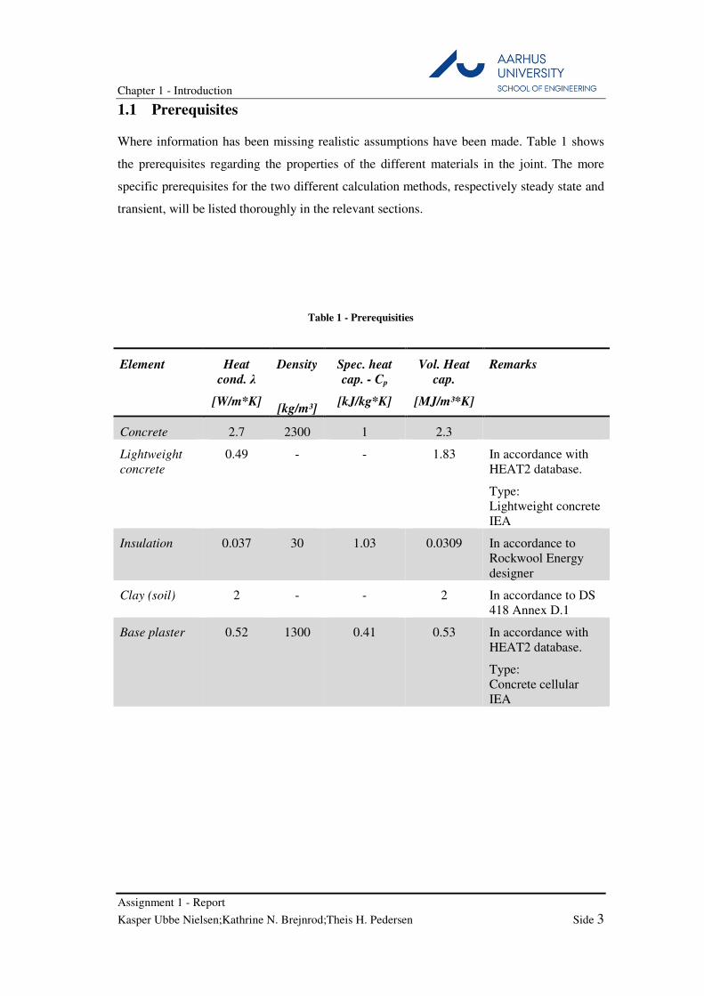
1.1 Prerequisites
Where information has been missing realistic assumptions have been made. Table 1 shows
the prerequisites regarding the properties of the different materials in the joint. The more
specific prerequisites for the two different calculation methods, respectively steady state and
transient, will be listed thoroughly in the relevant sections.
Table 1 - Prerequisities
Element Heat
cond. λ
[W/m*K]
Density
[kg/m³]
Spec. heat
cap. - Cp
[kJ/kg*K]
Vol. Heat
cap.
[MJ/m³*K]
Remarks
Concrete 2.7 2300 1 2.3
Lightweight
concrete
0.49 - - 1.83 In accordance with
HEAT2 database.
Type:
Lightweight concrete
IEA
Insulation 0.037 30 1.03 0.0309 In accordance to
Rockwool Energy
designer
Clay (soil) 2 - - 2 In accordance to DS
418 Annex D.1
Base plaster 0.52 1300 0.41 0.53 In accordance with
HEAT2 database.
Type:
Concrete cellular
IEA

Chapter 2 - Method
Assignment 1 - Report
Kasper Ubbe Nielsen;Kathrine N. Brejnrod;Theis H. Pedersen Side 5
2 Method
In the following section the methods used to calculate and evaluate the multidimensional,
one dimensional and linear heat loss coefficient is elaborated. The methods and prerequisites
described in DS 418 – section 6 (DS418, 2002), section 5.3 in Lecture Note on Thermal
Bridges (Petersen, 2013) and section 3.3.2 in Cold Bridges (Rode, 2001) is used in the
following calculation. Demands and further prerequisites that are not found in the above
literature are found in the Danish Building Regulation – §7.6 (Energistyrelsen, 2010). If not
found in the above, the source is stated at its relevance. Furthermore it is important to state
that the following calculations are based on internal measures.
2.1 Steady state condition
2.1.1 Method of modelling
2.1.1.1 Soil
The steady state situation only considers the one situation with a ∆T of 32 °C (Outdoor: -
12°C, Indoor: 20 °C), thereby no dynamics are considered. The modelling in HEAT2 is
based on the prerequisites mentioned in the above regarding surfaces resistances, though the
most important manner is the simplifications that is made regarding insulating effect of the
soil layer below and around the building part. Hence this is a steady state calculation, the
dynamic influence of the varying outdoor temperature are not concerned. In reality the deep
soil layer temperature is a function of the outdoor temperature and close to the mean outdoor
temperature if one digs deep enough and only observing the vertical heat flow (horizontal
boundary condition). If observing the near-field of the soil layer (still vertical heat flows),
under the building slab, this would be affected/warmed by the building, which differs from
the soil layers at same depth but under free ground. Regarding horizontal heat flows (vertical
boundary conditions), it is accepted to use an adiabatic boundary condition in a somewhat
far-field, this part is elaborated further in the following. Therefore a method of accounting
for the effect of the soil layers is needed. This manner is discussed in Cold Bridges (Rode,
2001) where three possible options are mentioned.
Chapter 2 - Method
Side 6 Assignment 1 - Report
Kasper Ubbe Nielsen;Kathrine N. Brejnrod;Theis H. Pedersen
Option 1 – The use of an adiabatic horizontal boundary condition at far-filed depths that
imitates the vanishing vertical heat flows at such depths.
Option 2 – The use of the mean annual outdoor temperature at some depth below the ground
as a horizontal boundary condition.
Option 3 – The use of the mean annual outdoor temperature at a depth equal to the depth,
that corresponds to the thermal resistance of the soil layer, as specified in DS 418,
amendment 4 (DS418, 2002), and the conductivity of the specific soil, as a horizontal
boundary condition.
Both option 1 and option 2 has their disadvantages. By implementing a horizontal adiabatic
boundary condition (Option 1) causes the temperature in the far-field of the soil to be a
function of the outdoor temperature, which, according to Appendix B.1, leads to a soil
temperature to cold and thereby a high and unrealistic heat loss towards the ground. Option 2
approaches a more realistic method, though not knowing the specific depth of where to place
the boundary condition may lead to imprecise and unrealistic results, hence if the depth is
chosen to small the temperature in the soil below the slab would be to warm, due to the lack
of influence of the outdoor temperature. If the depth is chosen to be too large, the same
situation as for option 1 occurs, where the temperature below the slab would be to cold, due
to too much influence of the outdoor temperature, according to Appendix B.2.
Option 3 accounts for the conductivity and the thermal resistance of the soil, by setting the
depth as a function of the two. This is, based on Appendix B.3, assessed to be the most
realistic method of the three, and thereby the method which is used the following calculation.
Chapter 2 - Method
Assignment 1 - Report
Kasper Ubbe Nielsen;Kathrine N. Brejnrod;Theis H. Pedersen Side 7
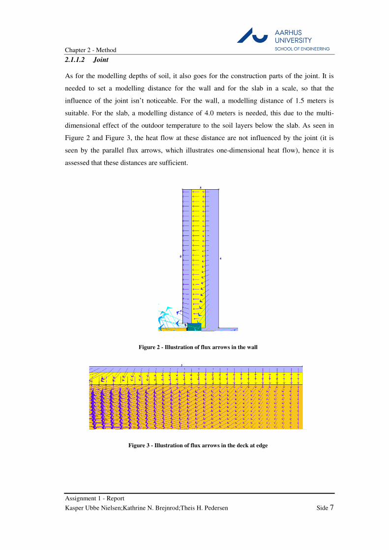
2.1.1.2 Joint
As for the modelling depths of soil, it also goes for the construction parts of the joint. It is
needed to set a modelling distance for the wall and for the slab in a scale, so that the
influence of the joint isn’t noticeable. For the wall, a modelling distance of 1.5 meters is
suitable. For the slab, a modelling distance of 4.0 meters is needed, this due to the multi-
dimensional effect of the outdoor temperature to the soil layers below the slab. As seen in
Figure 2 and Figure 3, the heat flow at these distance are not influenced by the joint (it is
seen by the parallel flux arrows, which illustrates one-dimensional heat flow), hence it is
assessed that these distances are sufficient.
Figure 2 - Illustration of flux arrows in the wall
Figure 3 - Illustration of flux arrows in the deck at edge
Chapter 2 - Method
Side 8 Assignment 1 - Report
Kasper Ubbe Nielsen;Kathrine N. Brejnrod;Theis H. Pedersen
2.1.2 Method of calculating
The way to calculate the heat loss through this joint is to observe the actual joint as a form of
lump that leads to a multidimensional heat flow, compared to the one-dimensional heat loss
through the homogenous constructions that are joined. This is best expressed in a linear-loss
coefficient, as a function of the length of the actual joint, in accordance with (EN ISO
10211-1, 1995). In a section like this, it is sufficient to calculate the multi-dimensional heat
loss as the two-dimensional (2D) heat loss.
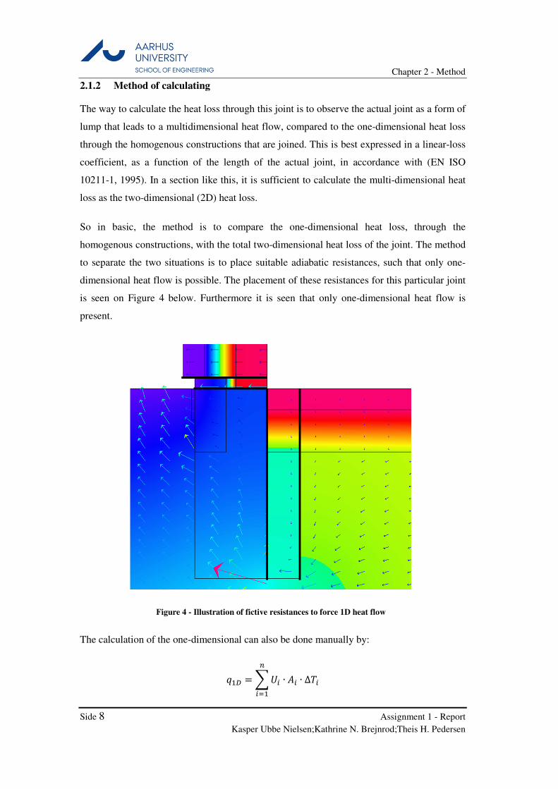
So in basic, the method is to compare the one-dimensional heat loss, through the
homogenous constructions, with the total two-dimensional heat loss of the joint. The method
to separate the two situations is to place suitable adiabatic resistances, such that only one-
dimensional heat flow is possible. The placement of these resistances for this particular joint
is seen on Figure 4 below. Furthermore it is seen that only one-dimensional heat flow is
present.
Figure 4 - Illustration of fictive resistances to force 1D heat flow
The calculation of the one-dimensional can also be done manually by:
��� ���� ∙ � ∙ ∆��
���

Chapter 2 - Method
Assignment 1 - Report
Kasper Ubbe Nielsen;Kathrine N. Brejnrod;Theis H. Pedersen Side 9
Next step is to choose suitable calculation-mesh that gives an adequate result. By adequate
meaning the relation of calculation time vs. precision of result. A criterion of for the
precision is stated in (EN ISO 10211-1, 1995) as a maximum change of heat flux of 1%
when comparing to meshes. Finally one has to subtract the calculated one-dimensional heat
loss from the calculated two-dimensional heat loss and divide it by the design temperature
difference used in the calculation.
2.2 Transient calculation
The linear heat loss coefficient for the joint is now determined based on transient simulations
according to the methodology of DS 418 appendix D.1 (DS418, 2002). In contrary to the
steady state method, the transient method takes the variations of the outdoor temperature and
thereby variations in the soil temperature into account.
2.2.1 Method of modelling
The 2D transient calculations are performed using the program HEAT2, ver. 8.03. The
model calculated is build up according to DS 418 appendix D.1, and is illustrated in Figure 5
with relevant temperatures, resistance and adiabatic boundaries. The current method
disregards heat flows in the foundations longitudinal direction at a distance of 4m from the
joint as well as heat flows through the adiabatic boundaries set at 20 meters below ground
and 20 meters left of the foundation.
Figure 5 - Transient model
Chapter 2 - Method
Side 10 Assignment 1 - Report
Kasper Ubbe Nielsen;Kathrine N. Brejnrod;Theis H. Pedersen
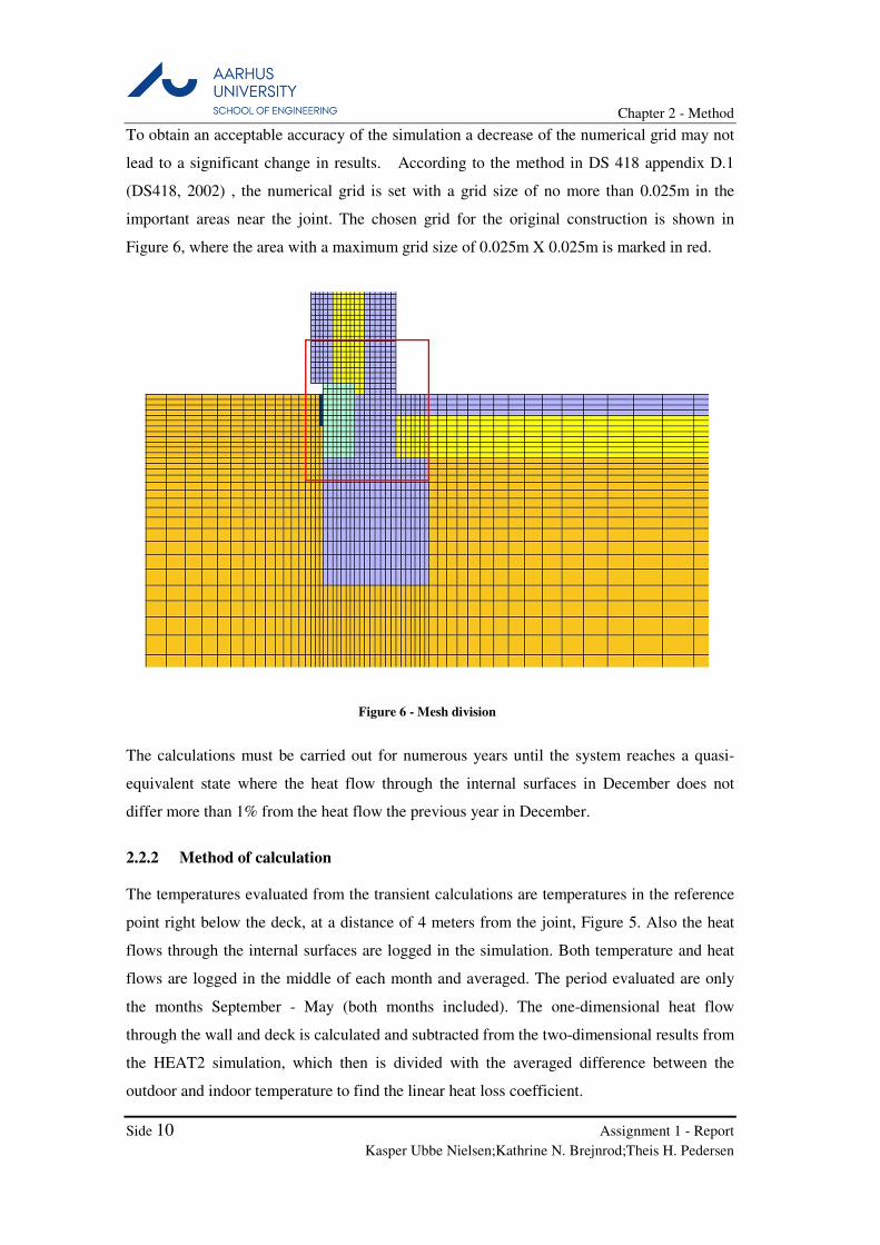
To obtain an acceptable accuracy of the simulation a decrease of the numerical grid may not
lead to a significant change in results. According to the method in DS 418 appendix D.1
(DS418, 2002) , the numerical grid is set with a grid size of no more than 0.025m in the
important areas near the joint. The chosen grid for the original construction is shown in
Figure 6, where the area with a maximum grid size of 0.025m X 0.025m is marked in red.
Figure 6 - Mesh division
The calculations must be carried out for numerous years until the system reaches a quasi-
equivalent state where the heat flow through the internal surfaces in December does not
differ more than 1% from the heat flow the previous year in December.
2.2.2 Method of calculation
The temperatures evaluated from the transient calculations are temperatures in the reference
point right below the deck, at a distance of 4 meters from the joint, Figure 5. Also the heat
flows through the internal surfaces are logged in the simulation. Both temperature and heat
flows are logged in the middle of each month and averaged. The period evaluated are only
the months September - May (both months included). The one-dimensional heat flow
through the wall and deck is calculated and subtracted from the two-dimensional results from
the HEAT2 simulation, which then is divided with the averaged difference between the
outdoor and indoor temperature to find the linear heat loss coefficient.
Chapter 2 - Method
Assignment 1 - Report
Kasper Ubbe Nielsen;Kathrine N. Brejnrod;Theis H. Pedersen Side 11
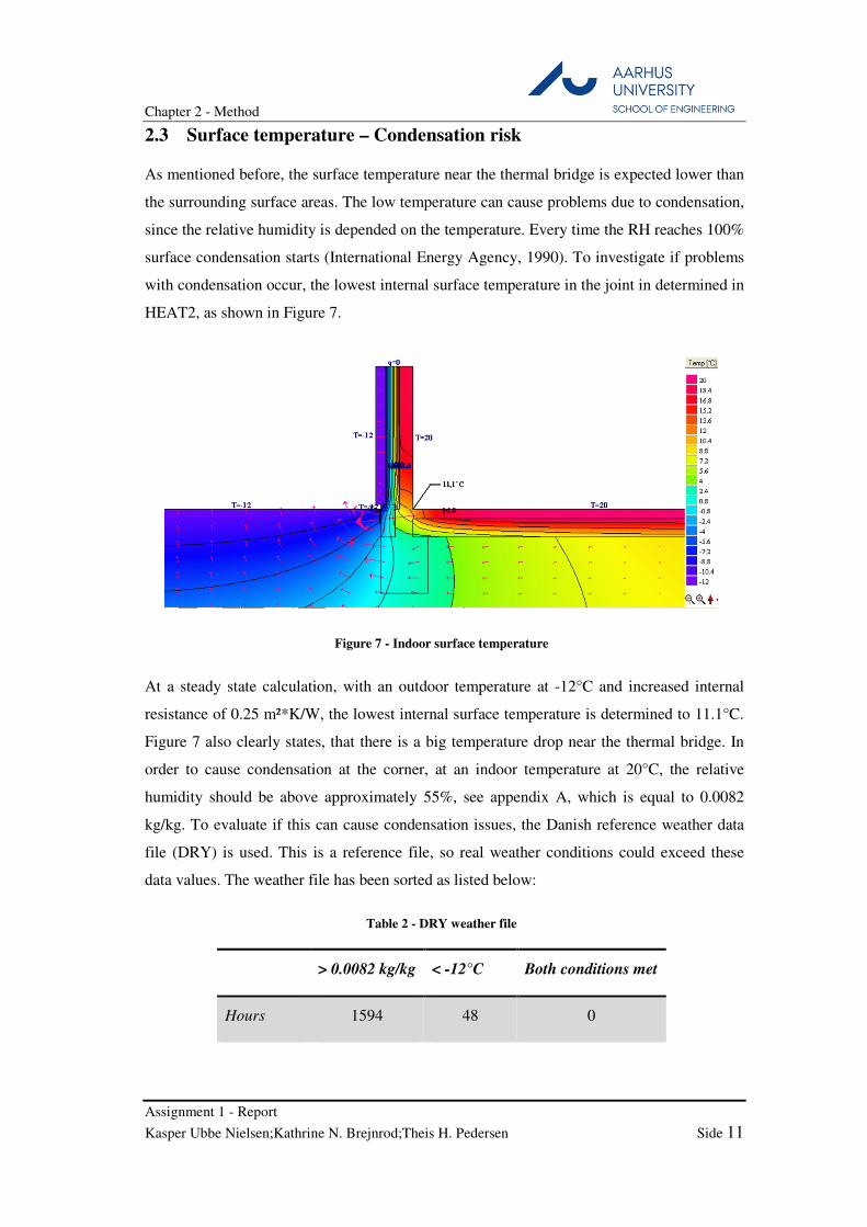
2.3 Surface temperature – Condensation risk
As mentioned before, the surface temperature near the thermal bridge is expected lower than
the surrounding surface areas. The low temperature can cause problems due to condensation,
since the relative humidity is depended on the temperature. Every time the RH reaches 100%
surface condensation starts (International Energy Agency, 1990). To investigate if problems
with condensation occur, the lowest internal surface temperature in the joint in determined in
HEAT2, as shown in Figure 7.
Figure 7 - Indoor surface temperature
At a steady state calculation, with an outdoor temperature at -12°C and increased internal
resistance of 0.25 m²*K/W, the lowest internal surface temperature is determined to 11.1°C.
Figure 7 also clearly states, that there is a big temperature drop near the thermal bridge. In
order to cause condensation at the corner, at an indoor temperature at 20°C, the relative
humidity should be above approximately 55%, see appendix A, which is equal to 0.0082
kg/kg. To evaluate if this can cause condensation issues, the Danish reference weather data
file (DRY) is used. This is a reference file, so real weather conditions could exceed these
data values. The weather file has been sorted as listed below:
Table 2 - DRY weather file
> 0.0082 kg/kg < -12°C Both conditions met
Hours 1594 48 0
Chapter 2 - Method
Side 12 Assignment 1 - Report
Kasper Ubbe Nielsen;Kathrine N. Brejnrod;Theis H. Pedersen
Table 2 indicates that condensations cannot occur directly based on the outdoor conditions,
since both demands are not fulfilled at the same time. The reason is that low temperature air
cannot contain as much water as warmer air. However as mentioned previously, the true
weather conditions can differ from the reference file.
Furthermore, an even more important parameter is the human production of water by
exhaling. If two people are sleeping in a small room, without any ventilation, the content of
water in the air could easily exceed RH 55%. To prevent risk of condensation, and thereby
moisture related problems, it is therefore important to ventilate frequently.
Chapter 3 - Results
Assignment 1 - Report
Kasper Ubbe Nielsen;Kathrine N. Brejnrod;Theis H. Pedersen Side 13
3 Results
3.1 Original model
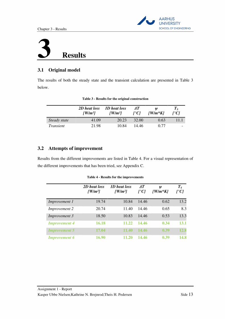
The results of both the steady state and the transient calculation are presented in Table 3
below.
Table 3 - Results for the original construction
2D heat loss
[W/m²]
1D heat loss
[W/m²]
∆T
[°C]
ψ
[W/m*K]
TS
[°C]
Steady state 41.09 20.23 32.00 0.63 11.1
Transient 21.98 10.84 14.46 0.77 -
3.2 Attempts of improvement
Results from the different improvements are listed in Table 4. For a visual representation of
the different improvements that has been tried, see Appendix C.
Table 4 - Results for the improvements
2D heat loss
[W/m²]
1D heat loss
[W/m²]
∆T
[°C]
ψ
[W/m*K]
TS
[°C]
Improvement 1 19.74 10.84 14.46 0.62 13.2
Improvement 2 20.74 11.40 14.46 0.65 8.3
Improvement 3 18.50 10.83 14.46 0.53 13.3
Improvement 4 16.18 11.22 14.46 0.34 13.1
Improvement 5 17.04 11.40 14.46 0.39 12.8
Improvement 6 16.90 11.20 14.46 0.39 14.8


Chapter 4 - Analysis & Discussion
Assignment 1 - Report
Kasper Ubbe Nielsen;Kathrine N. Brejnrod;Theis H. Pedersen Side 15
4 Analysis & Discussion
4.1 Steady state calculation vs. Transient simulation
The obvious differences of the two methods are given by their respective names. The steady
state solution is a numerical calculation of a “snapshot” incident with a given set of static
boundary conditions. The transient simulation is a numerical calculation representing a
defined timeframe, often a year, which is affected by dynamic boundary conditions that vary
with time, where the calculation is performed for a certain time step including a set of
parameters from the former time step. As it indicates, the time it takes to perform the two
solutions differs a lot. Both solution methods increase in calculation- and simulation time as
the previously mentioned mesh is increased. The error criterion also affects the time, hence
the number of iterations increase.
When to use what? It of course depends of the question asked. The steady state calculation is
a quick method to make a benchmark solution of a given solution, whereas the transient
simulation is a more time consuming, but also precise solution, this of course depends on the
input that is given to the model. For example one could argue whether it is correct or not to
apply a static indoor temperature to the transient model, where a dynamic outdoor
temperature is used.

Chapter 4 - Analysis & Discussion
Side 16 Assignment 1 - Report
Kasper Ubbe Nielsen;Kathrine N. Brejnrod;Theis H. Pedersen
4.2 Original construction
4.2.1 Heat loss
As stated in Chapter 3, the linear heat loss coefficient through the joint in the original
construction of Ψ = 0.77 W/mK does not comply with the legal requirements of the danish
building regulations on 0.40 W/mK (Energistyrelsen, 2010, 7.6. stk 1).
Figure 8 - Original construction
The high linear heat loss coefficient is due to the huge constructional thermal bridges caused
by the exposed foundation block. As Figure 8 illustrates the heat is easily transmitted from
the deck- and bearing wall elements through the foundation block since no insulation is
“breaking” the thermal bridge, and the extra heat loss through the corner is therefore
considerably.
4.3 Alternative build-ups
To improve the construction, decrease the linear heat loss coefficient and increase the
minimum surface temperature, the thermal bridge must be broken. The impact of several
improvements has been investigated in order to develop a joint that fulfill the Danish
Building Regulations. The improvements are listed in Appendix C.
It is shown from the results that in order to reduce the heat loss through the joint, the break in
insulation has to be eliminated.
Chapter 4 - Analysis & Discussion
Assignment 1 - Report
Kasper Ubbe Nielsen;Kathrine N. Brejnrod;Theis H. Pedersen Side 17
As shown at improvement 2 and 6, the minimum surface temperature is greatly affected by
the addition of a small insulation wedge, placed just between the corner and the ground floor.
Unlike the other improvements of the linear heat loss coefficient, this will reduce the
minimal surface temperature. The reason for this is that the heat flux that previously went
through the slap is being prevented to reach the corner point. The reason why the internal
minimum temperature for the other improvements still exceeds the original temperature is
due to the overall reduction of the linear heat transmission.
The simulations of the different alterations have also shown, that it is more effective to place
the insulating layer as close to the thermal bridge as possible. It is therefore more effective to
place the insulation in between the Leca blocks, than on the outside.
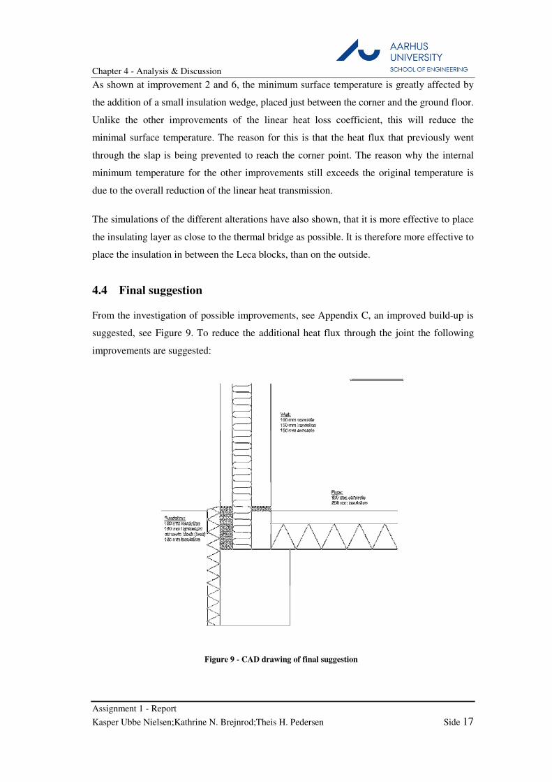
4.4 Final suggestion
From the investigation of possible improvements, see Appendix C, an improved build-up is
suggested, see Figure 9. To reduce the additional heat flux through the joint the following
improvements are suggested:
Figure 9 - CAD drawing of final suggestion
Chapter 4 - Analysis & Discussion
Side 18 Assignment 1 - Report
Kasper Ubbe Nielsen;Kathrine N. Brejnrod;Theis H. Pedersen
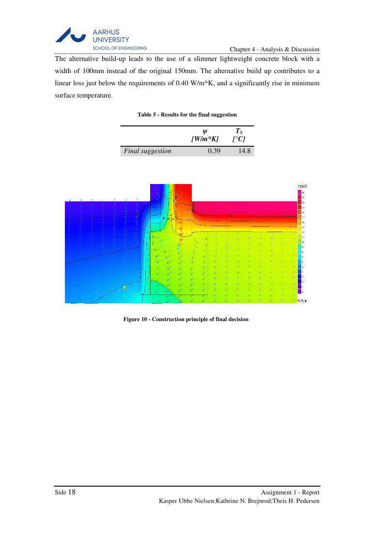
The alternative build-up leads to the use of a slimmer lightweight concrete block with a
width of 100mm instead of the original 150mm. The alternative build up contributes to a
linear loss just below the requirements of 0.40 W/m*K, and a significantly rise in minimum
surface temperature.
Table 5 - Results for the final suggestion
ψ
[W/m*K]
TS
[°C]
Final suggestion 0.39 14.8
Figure 10 - Construction principle of final decision

Chapter 5 - Conclusion
Assignment 1 - Report
Kasper Ubbe Nielsen;Kathrine N. Brejnrod;Theis H. Pedersen Side 19
5 Conclusion
In order to minimize the overall heat transmission loss, the Danish Building Regulation
states a demand of a maximum linear heat coefficient at 0.40 W/m*K. The original build-up
of the joint had a coefficient of 0.77 W/m*k which exceeded the demand greatly, and at the
same time the minimum surface temperature of 11.1°C could lead to problems related to
condensation and thereby mold issues.
Different improvements have been tested, in order to evaluate the performance on the linear
coefficient. A final suggestion has been made, which both favor the internal minimum
surface temperature and the linear heat coefficient. The alternative build-up includes external
insulation and a continuation of the wall insulation and leads to a linear heat loss coefficient
of 0.39 W/m*K and a minimum surface temperature of 14.8°C. The alternative build-up
thereby satisfies the legal requirements to the linear heat loss coefficient and issues related to
moisture are prevented.
There has been performed both steady state calculations and transient simulations, to
determine the accuracy and usability of the one compared to the other. As described in
chapter 4.1, the methods have different pros and cons. In the case, we have found that the
steady state calculation is obvious for a benchmark of different solutions, due to the low
calculation time. The transient simulation is more time consuming, however the result is
more correct, and the method should therefore be used for determination of the linear
coefficient, as also stated in the Danish Standard 418 (DS418, 2002).

Chapter 6 - Bibliography
Assignment 1 - Report
Kasper Ubbe Nielsen;Kathrine N. Brejnrod;Theis H. Pedersen Side 21
6 Bibliography
DS418, 2002. Beregninger af bygningers varmetab, København: Dansk Standard.
EN ISO 10211-1, 1995. EN ISO 10211-1:1995, s.l.: s.n.
Energistyrelsen, 2010. Bygningsreglementet 2010. [Online]
Available at: www.bygningsreglementet.dk
International Energy Agency, 1990. Guidlines & Practice Vol. 2 - Annex 14 "Condensation
and Energy", s.l.: IEA.
Petersen, S., 2013. Lecture note on Thermal Bridges, Aarhus: Aarhus University Department
of Engineering.
Rode, C., 2001. Cold Bridges, s.l.: Department of Civil Engineering Technical University of
Denmark.

Chapter 7 - Appendix
Assignment 1 - Report
Kasper Ubbe Nielsen;Kathrine N. Brejnrod;Theis H. Pedersen Side 23
7 Appendix
Appendix A IX-diagram ....................................................................................................... 1
Appendix B Assessment of options ...................................................................................... 3
Appendix C Attempts of improvements ............................................................................... 7


Chapter 7 - Appendix
Assignment 1 - Report
Kasper Ubbe Nielsen;Kathrine N. Brejnrod;Theis H. Pedersen Side 1
Appendix A IX-diagram
Indoor temperature: 20°C
Relative humidity: 60%
Dew point temperature: 12°C


Chapter 7 - Appendix
Assignment 1 - Report
Kasper Ubbe Nielsen;Kathrine N. Brejnrod;Theis H. Pedersen Side 3
Appendix B Assessment of options
In the following sections, measurements of the soil temperature at different depths has been
performed, compared and assessed to determine whether the chosen option is a realistic
representation of the soil temperature in a steady state calculation.
Appendix B.1 Option 1
In the following section Option 1 from Cold Bridges (Rode, 2001) is assessed regarding a
realistic representation of the soil temperature in a steady state calculation.
Far field adiabatic case Appendix B.1.1
From Figure 11 and Table 6 it is obvious that the soil temperature in every layer is below
0°C and thereby too cold to give a realistic representation of the soil temperature.
Figure 11 - Temperature plot far field adiabatic case. Source: HEAT2
Table 6 - Temperature for Far field adiabatic case
Temperature
[°C]
Below insulation -1.16
1 meter depth -2.88
3 meters depth -5.33
20 meters depth -9.21
Chapter 7 - Appendix
Side 4 Assignment 1 - Report
Kasper Ubbe Nielsen;Kathrine N. Brejnrod;Theis H. Pedersen
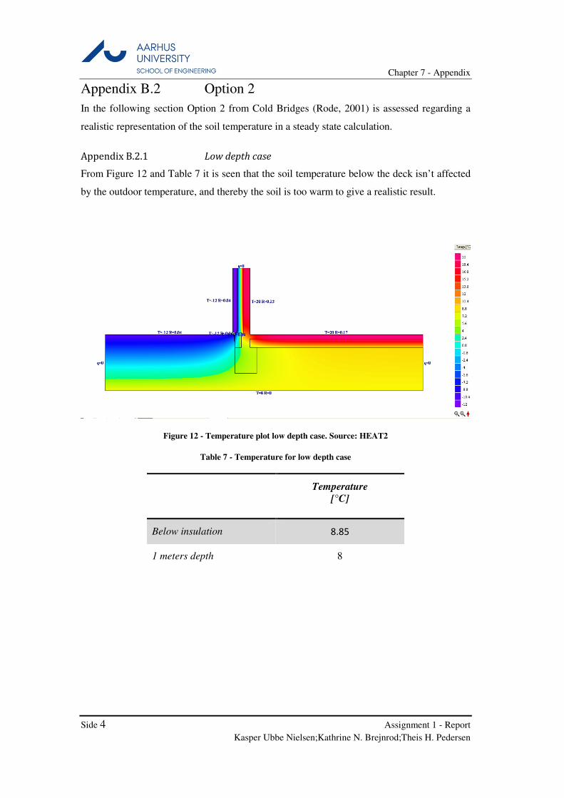
Appendix B.2 Option 2
In the following section Option 2 from Cold Bridges (Rode, 2001) is assessed regarding a
realistic representation of the soil temperature in a steady state calculation.
Low depth case Appendix B.2.1
From Figure 12 and Table 7 it is seen that the soil temperature below the deck isn’t affected
by the outdoor temperature, and thereby the soil is too warm to give a realistic result.
Figure 12 - Temperature plot low depth case. Source: HEAT2
Table 7 - Temperature for low depth case
Temperature
[°C]
Below insulation 8.85
1 meters depth 8
Chapter 7 - Appendix
Assignment 1 - Report
Kasper Ubbe Nielsen;Kathrine N. Brejnrod;Theis H. Pedersen Side 5
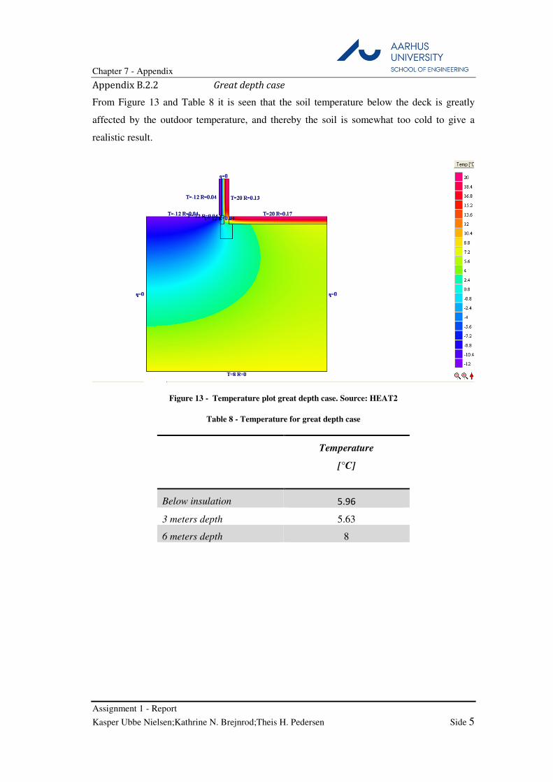
Great depth case Appendix B.2.2
From Figure 13 and Table 8 it is seen that the soil temperature below the deck is greatly
affected by the outdoor temperature, and thereby the soil is somewhat too cold to give a
realistic result.
Figure 13 - Temperature plot great depth case. Source: HEAT2
Table 8 - Temperature for great depth case
Temperature
[°C]
Below insulation 5.96
3 meters depth 5.63
6 meters depth 8

Chapter 7 - Appendix
Side 6 Assignment 1 - Report
Kasper Ubbe Nielsen;Kathrine N. Brejnrod;Theis H. Pedersen
Appendix B.3 Option 3
In the following section Option 3 from Cold Bridges (Rode, 2001) is assessed regarding a
realistic representation of the soil temperature in a steady state calculation.
Conduction VS. resistance case Appendix B.3.1
From Figure 14 and Table 9 it is clearly seen that the temperature of the soil is represented in
a somewhat more realistic manner regarding the temperature plot.
Figure 14 - Temperature plot conduction vs. resistance case. Source: HEAT2
Table 9 - Temperature for conduction vs. resistance case
Temperature
[°C]
Below insulation 8.34
1 meter depth 7.4
3 meters depth 8.03
Chapter 7 - Appendix
Assignment 1 - Report
Kasper Ubbe Nielsen;Kathrine N. Brejnrod;Theis H. Pedersen Side 7
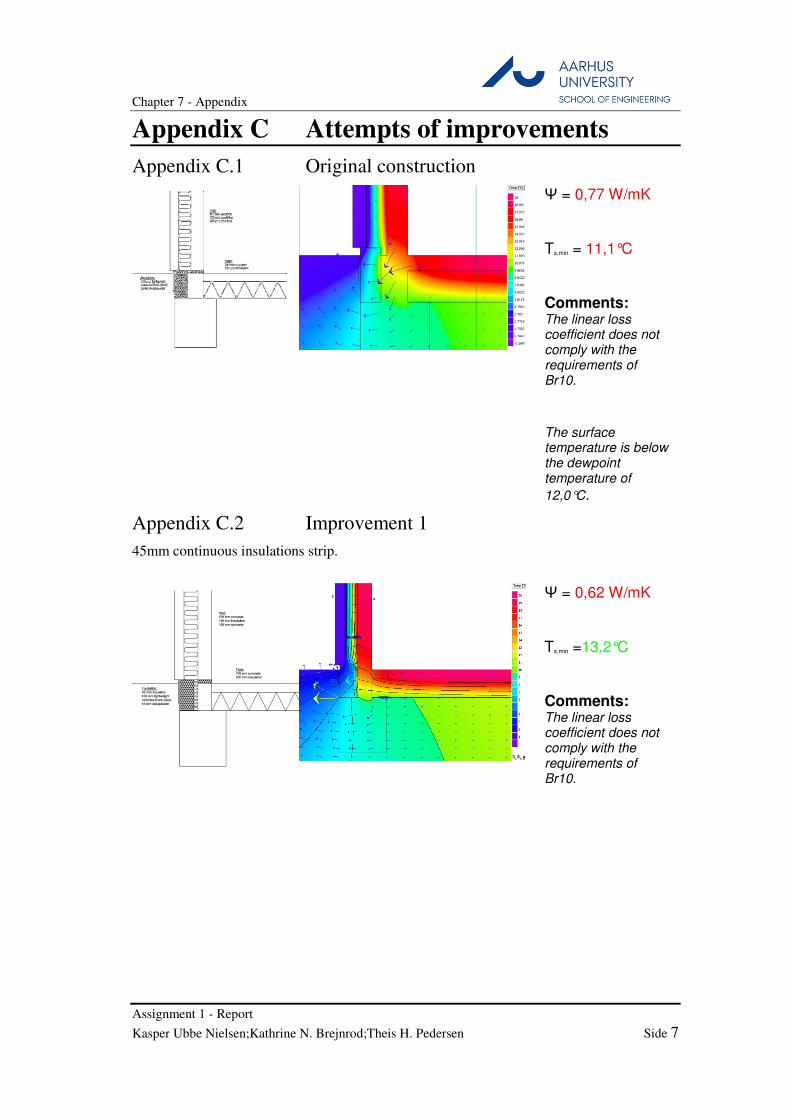
Appendix C Attempts of improvements
Appendix C.1 Original construction
Ψ = 0,77 W/mK
Ts,min = 11,1°C
Comments: The linear loss coefficient does not comply with the requirements of Br10.
The surface temperature is below the dewpoint temperature of
12,0°C.
Appendix C.2 Improvement 1
45mm continuous insulations strip.
Ψ = 0,62 W/mK
Ts,min =13,2°C
Comments: The linear loss coefficient does not comply with the requirements of Br10.
Chapter 7 - Appendix
Side 8 Assignment 1 - Report
Kasper Ubbe Nielsen;Kathrine N. Brejnrod;Theis H. Pedersen
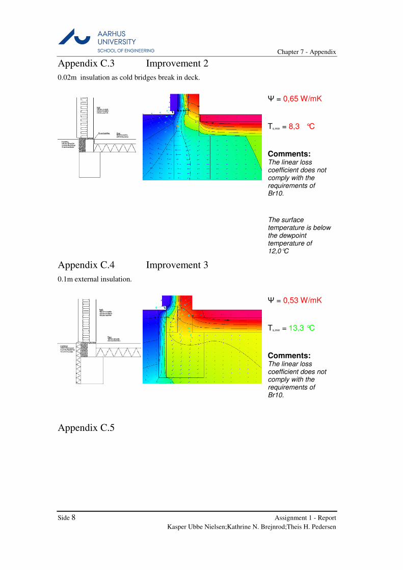
Appendix C.3 Improvement 2
0.02m insulation as cold bridges break in deck.
Ψ = 0,65 W/mK
Ts,min = 8,3 °C
Comments: The linear loss coefficient does not comply with the requirements of Br10.
The surface temperature is below the dewpoint temperature of 12,0°C
Appendix C.4 Improvement 3
0.1m external insulation.
Ψ = 0,53 W/mK
Ts,min = 13,3 °C
Comments: The linear loss coefficient does not comply with the requirements of Br10.
Appendix C.5
Chapter 7 - Appendix
Assignment 1 - Report
Kasper Ubbe Nielsen;Kathrine N. Brejnrod;Theis H. Pedersen Side 9
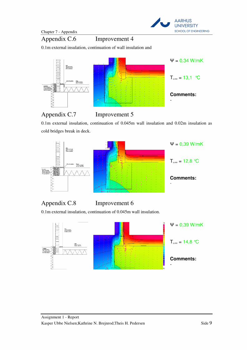
Appendix C.6 Improvement 4
0.1m external insulation, continuation of wall insulation and
Ψ = 0,34 W/mK
Ts,min = 13,1 °C
Comments: -
Appendix C.7 Improvement 5
0.1m external insulation, continuation of 0.045m wall insulation and 0.02m insulation as
cold bridges break in deck.
Ψ = 0,39 W/mK
Ts,min = 12,8 °C
Comments: -
Appendix C.8 Improvement 6
0.1m external insulation, continuation of 0.045m wall insulation.
Ψ = 0,39 W/mK
Ts,min = 14,8 °C
Comments: -