Heat and Mass Transfer of a Low Pressure Mars Greenhouse...
146
HEAT AND MASS TRANSFER OF A LOW PRESSURE MARS GREENHOUSE: SIMULATION AND EXPERIMENTAL ANALYSIS By INKA HUBLITZ A DISSERTATION PRESENTED TO THE GRADUATE SCHOOL OF THE UNIVERSITY OF FLORIDA IN PARTIAL FULFILLMENT OF THE REQUIREMENTS FOR THE DEGREE OF DOCTOR OF PHILOSOPHY UNIVERSITY OF FLORIDA 2006
Transcript of Heat and Mass Transfer of a Low Pressure Mars Greenhouse...

HEAT AND MASS TRANSFER OF A LOW PRESSURE MARS GREENHOUSE:
SIMULATION AND EXPERIMENTAL ANALYSIS
By
INKA HUBLITZ
A DISSERTATION PRESENTED TO THE GRADUATE SCHOOL OF THE UNIVERSITY OF FLORIDA IN PARTIAL FULFILLMENT
OF THE REQUIREMENTS FOR THE DEGREE OF DOCTOR OF PHILOSOPHY
UNIVERSITY OF FLORIDA
2006

Copyright 2006
by
Inka Hublitz

I dedicate this dissertation to my parents, Melitta and Bruno Hublitz, who have always supported my adventures and endeavors. Their love and guidance encouraged me to follow my dreams and to reach innumerable goals.

iv
ACKNOWLEDGMENTS
First and foremost, I would like to express my deepest gratitude to my major
advisor, Dr. Ray Bucklin, for giving me the unique opportunity to complete my Ph.D.
program under his guidance. Furthermore, I am thankful that Dr. Bucklin encouraged me
to participate in various conferences and international events, such as the International
Space University’s Summer Session Program in Australia. With his help I have
constantly increased my network of colleagues working in relevant fields. Dr. Bucklin’s
help in realizing my stay at NASA’s Kennedy Space Center was also highly appreciated.
I also acknowledge the members of my supervisory committee for their huge
amount of support and advice. I especially would like to thank
• Dr. Jim Leary for his positive attitude that helped me enrich my people skills.
• Dr. Khe Chau for providing me with lab space.
• Dr. Raymond Wheeler for introducing me to Dr. Bucklin during my master’s thesis research and for helping to organize my stay at NASA’s Kennedy Space Center.
• Dr. David Hahn for his quick responses to all my questions and for being much more involved in the project than an external committee member generally is.
I am grateful to Dr. Sencer Yeralan for sharing his great expertise in the field of
microcontrollers. At NASA’s Kennedy Space Center I thank Dr. Vadim Rygalov, Dr.
Phil Fowler and Dr. John Sager for their support. I am thankful to Dr. Hartwell Allen for
teaching me how to grow plants and providing me with the right equipment. Bob
Tonkinson’s, Billy Duckworth’s and Steve Feagle’s hard work was always greatly
appreciated.

v
My family and my husband, Sharath Cugati, deserve special thanks for their
emotional and technical support. My gratitude also extends to my friends Dr. Peter Eckart
and Dr. Kristian Pauly, for introducing me to the field of space life support systems and
biospherics.

vi
TABLE OF CONTENTS page
ACKNOWLEDGMENTS ................................................................................................. iv
LIST OF TABLES............................................................................................................. ix
LIST OF FIGURES ........................................................................................................... xi
ABSTRACT.......................................................................................................................xv
CHAPTER
1 INTRODUCTION ........................................................................................................1
Low Pressure Mars Greenhouses..................................................................................1 Structure of the Dissertation .........................................................................................3
2 LITERATURE REVIEW .............................................................................................4
Advanced Life Support.................................................................................................4 Mars Environment ........................................................................................................6 Plant Requirements and Environment Control ...........................................................10
Temperature.........................................................................................................11 Temperature effect .......................................................................................11 Temperature control .....................................................................................12
Relative Humidity ...............................................................................................12 Relative humidity effect ...............................................................................12 Relative humidity control.............................................................................13
Atmospheric Pressure and Composition .............................................................13 Carbon dioxide effect ...................................................................................13 Carbon dioxide control.................................................................................14 Oxygen effect ...............................................................................................14 Oxygen control .............................................................................................15 Vapor pressure effect and control ................................................................15 Pressurizing gas............................................................................................15
Ventilation ...........................................................................................................15 Radiation..............................................................................................................16
Radiation effects...........................................................................................16 Radiation control ..........................................................................................17
Growth Area ........................................................................................................19

vii
Low Pressure Plant Growth Studies ...........................................................................19
3 OBJECTIVES OF THIS STUDY ..............................................................................23
4 EXPERIMENTAL WORK ........................................................................................24
System Description.....................................................................................................24 Instrumentation and Sensor Calibration .....................................................................28 Leakage Testing..........................................................................................................32
Leakage of Vacuum Chamber .............................................................................32 Leakage of Greenhouse Dome ............................................................................34
Data Acquisition and Control System ........................................................................36 Greenhouse Dome Environmental Control ................................................................37
Gas Composition and Total Pressure Control Algorithm....................................37 Air Temperature Control Algorithm ...................................................................39
Heat and Mass Transfer Experiments without Plants.................................................41 Heat and Mass Transfer Experiments with Plants......................................................50
Medium-term Plant Experiment involving Buttercrunch Lettuce.......................50 Long-term Plant Experiment involving Galactic Lettuce ...................................56
5 MATHEMATICAL MODEL DEVELOPMENT ......................................................65
Effect of Low Pressure on Heat and Mass Transfer ...................................................65 Convection Heat Transfer....................................................................................65
Laminar flow over a horizontal plate ...........................................................67 Turbulent flow over a horizontal plate .........................................................68 Laminar free convection on a vertical plate .................................................69 External free convection for a sphere...........................................................70
Mass Transfer by Evaporation.............................................................................71 Development of Low Pressure Psychrometrics for Non-Standard Atmospheres.......72
Gas Theory ..........................................................................................................73 Equation of state...........................................................................................73 Dry gas mixture............................................................................................74 Water vapor component ...............................................................................75
Construction of Modified Psychrometric Chart ..................................................75 Saturation line ..............................................................................................75 Humidity isolines .........................................................................................77 Specific enthalpy isolines.............................................................................78 Specific volume isolines...............................................................................78 Vapor pressure isolines ................................................................................79 Adiabatic saturation temperature isolines ....................................................79 Dew-point temperature isolines ...................................................................80
One–dimensional Steady State Heat Transfer Model of the Greenhouse Dome........83 Overall Thermal Resistance Model .....................................................................83 Individual Thermal Resistances and Thermal Coefficients.................................84 Total Thermal Resistance ....................................................................................90 Comparison of Radiation and Convection in the Chamber at Mars Pressure .....92

viii
Transient Heat Transfer Model for Greenhouse Temperature Simulation.................93
6 RESULTS AND CONCLUSION...............................................................................98
7 FUTURE WORK......................................................................................................100
APPENDIX
A STRUCTURAL ANALYSIS OF DOME SHELL, BASE PLATE AND CYLINDRICAL CALIBRATION CHAMBER ......................................................102
Structural Analysis of the Spherical Greenhouse Dome ..........................................102 Structural Analysis of Base Plate for Greenhouse Dome.........................................103
Structural Analysis of the Base Plate without Additional Bracings..................104 Structural Analysis of the Base Plate with Additional Bracings.......................106
Structural Analysis of Cylinder used as Sensor Calibration Chamber .....................112 Maximum Allowable Pressure ..........................................................................112
Short cylinder behavior ..............................................................................113 Intermediate cylinder behavior...................................................................113 Long cylinder behavior ..............................................................................114
Axial Buckling...................................................................................................114 Wall Yielding ....................................................................................................115
B SENSOR CALIBRATION.......................................................................................116
Pressure.....................................................................................................................116 Temperature..............................................................................................................117 Relative Humidity.....................................................................................................117 Carbon Dioxide Concentration .................................................................................118 Oxygen Concentration ..............................................................................................119 Load Cells.................................................................................................................121 Radiation...................................................................................................................122 Amplification of Low Voltage Sensors ....................................................................123
LIST OF REFERENCES.................................................................................................124
BIOGRAPHICAL SKETCH ...........................................................................................129

ix
LIST OF TABLES
Table page 2-1 Human metabolism values per crew member and per day (CM-d) for average
activity level. ..............................................................................................................5
2-2 Environment properties. .............................................................................................8
2-3 Atmosphere composition by volume..........................................................................8
2-4 Plant environment requirements...............................................................................10
2-5 Advanced life support crop growth conditions. .......................................................11
4-1 Sensors used to measure environmental parameters, the sensor ranges and accuracies. ................................................................................................................29
4-2 Steady state temperature distribution under different freezer temperature, light and heating power conditions...................................................................................44
4-3 Buttercrunch lettuce environmental conditions and their control. ...........................53
4-4 Evaporation rates per scale with scales 2-5 containing two lettuce plants each. .....55
4-5 Galactic lettuce environmental conditions and their control....................................57
5-1 Effect of reduced pressure on convective heat transfer coefficient and mass diffusion coefficient. ................................................................................................71
5-2 Psychrometric parameters of a low pressure atmosphere (76% N2, 20% O2, 4% CO2) with initial conditions of 20 kPa dry air at 20°C and a constant specific volume of 0.004138m³/kg. .......................................................................................80
5-3 Steady state temperature data of the long-term experiment involving Galactic lettuce plants.............................................................................................................86
5-4 Thermal resistances and coefficients based on the data obtained of the long-term experiment involving Galactic lettuce plants. ..........................................................87
5-5 Simulated temperatures based on the thermal resistance model. .............................89
5-6 Comparison of measured and simulated temperature values. ..................................90

x
5-7 Comparison of convection heat transfer to radiation heat transfer in the chamber at a pressure of 0.6 kPa.............................................................................................93
A-1 Structural analysis of base plate without and with additional bracings. ................112

xi
LIST OF FIGURES
Figure page 1-1 "Astronaut" approaching University of Florida’s Mars Greenhouse Dome. .............2
2-1 Martian spectral irradiance (Ls=250, 15ºS, noon) vs. terrestrial spectral irradiance....................................................................................................................9
2-2 Average solar irradiance of Mars compared to Earth...............................................10
2-3 Photosynthetic efficiency .........................................................................................16
4-1 Dome used to protect plants from the simulated low pressure, low temperature Mars environment. A) Empty dome. B) Dome with sensors, scales and flasks installed. ...................................................................................................................25
4-2 Vacuum chamber used to simulate the low pressure Mars environment (less than 1% of Earth’s atmosphere). ......................................................................................26
4-3 Industrial walk-in freezer ensures low temperature of the vacuum chamber (simulated Mars environment). ................................................................................26
4-4 Schematic of experimental setup..............................................................................28
4-5 Cylinder used for calibration of pressure-sensitive sensors and for initial gas mixing control algorithm development. ...................................................................30
4-6 Comparison of Honeywell capacitance RH sensors to the HMP 237 reference RH sensor for pressures of 0 to 25 kPa. ...................................................................31
4-7 Forces on chamber window. A) Vacuum chamber at 0.6 kPa with top window bulging in. B) Gasket drawn into the chamber due to pressure difference. .............33
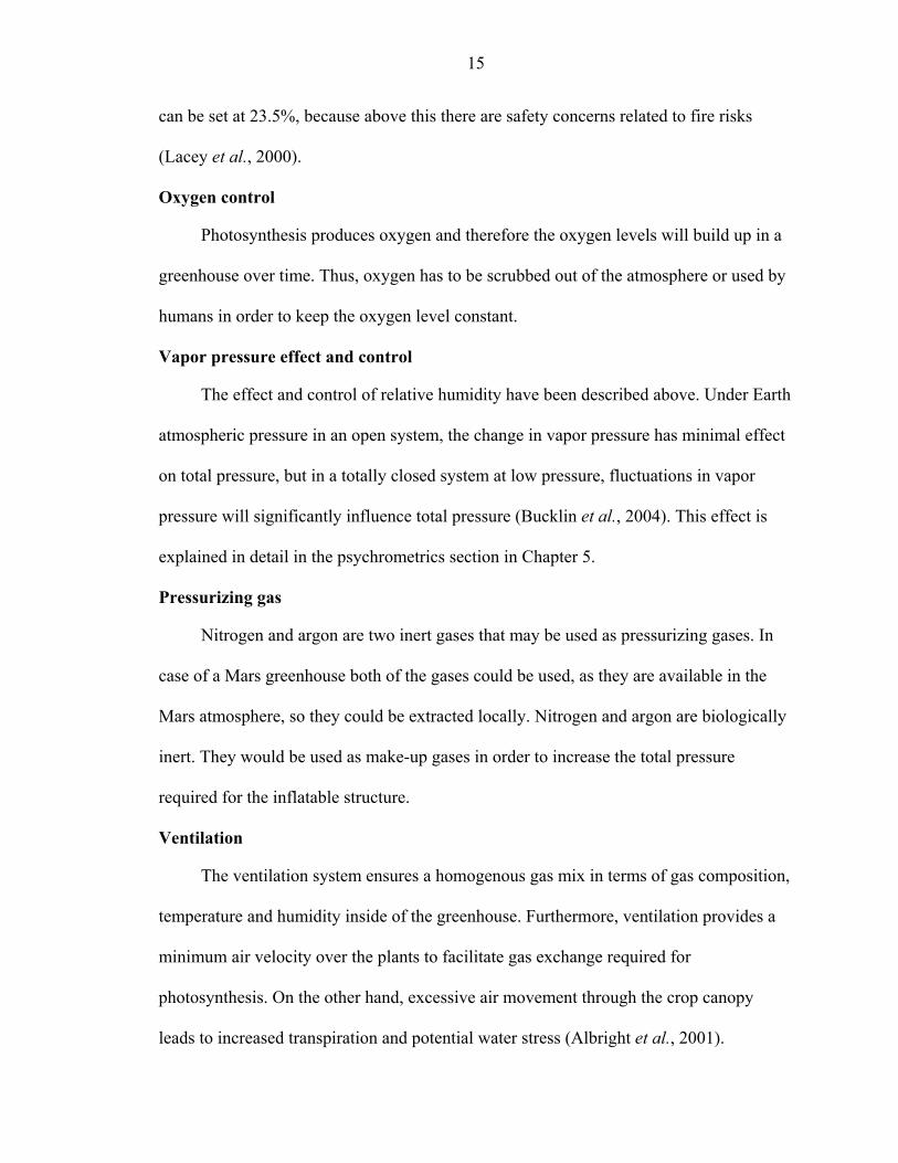
4-8 Dome and chamber leakage with gas resupply and vacuum pumps turned off at a temperature of -10 ºC. ..............................................................................................35
4-9 Comparison of vacuum chamber and greenhouse dome leak rates to values of other low pressure plant growth studies (leak rate is presented in logarithmic scale).........................................................................................................................35
4-10 Gas mixing of dome greenhouse atmosphere without plants (oxygen set point at 4.0 kPa and carbon dioxide set point at 0.5 kPa). ....................................................38

xii
4-11 Pressure control of vacuum chamber (set point 0.6 kPa) and greenhouse dome (set points 20 kPa). ...................................................................................................39
4-12 Air temperature control of greenhouse dome (set point at 20 ºC)............................40
4-13 Sensor locations for heat and mass transfer experiments without plants. ................41
4-14 Preparation of the steady state experiments. A) Bottom of dome base with foam insulation. B) Side view of greenhouse dome with the sensors and scales installed. C) Top view of greenhouse dome without shell. D) Installation of greenhouse dome into the vacuum chamber. ...........................................................42
4-15 Temperature readings until steady state is achieved. (0 ºC freezer temperature, 26 W heating power and light switched off). ...........................................................43
4-16 Steady state temperatures versus power of heater at seven different locations (T1-T7). Freezer temperature is 0 ºC and the growth light is switched off...............44
4-17 Steady state temperatures versus power of heater at seven different locations (T1-T7). Freezer temperature is -10 ºC and the growth light is switched off. ..........45
4-18 Steady state temperatures versus power of heater at seven different locations (T1-T7). Freezer temperature is -20 ºC and the growth light is switched off. ..........45
4-19 Steady state temperatures versus power of heater at seven different locations (T1-T7). Freezer temperature is -10 ºC and the growth light is switched on. ...........46
4-20 Steady state temperatures versus power of heater at seven different locations (T1-T7). Freezer temperature is -20 ºC and the growth light is switched on. ...........46
4-21 Steady state air temperatures (T3) versus power of heater for freezer temperatures of 0 ºC, -10 ºC and -20 ºC (growth light switched off).......................47
4-22 Freezer temperature versus power of heater for steady state air temperatures (T3) of 15 ºC, 20 ºC and 25 ºC. ........................................................................................48
4-23 Condensation inside of greenhouse shell with a greenhouse air temperature of 20 ºC. A) Freezer temperature at 0 ºC. B) Freezer temperature at -20 ºC.....................50
4-24 Buttercrunch lettuce in Ehrlenmeyer flask. A) The average height of the shoot zone is 15 cm. B) Putty and a stopper prevent evaporation of the hydroponic solution as they separate the root from the shoot zone. ...........................................51
4-25 Installation of flasks containing the lettuce plants onto the scales...........................52
4-26 Constant temperature distribution and varying relative humidity during the buttercrunch lettuce experiment. ..............................................................................53

xiii
4-27 Plant evapo-transpiration rates of plants from 5 to 10 hours after the beginning of the experiment......................................................................................................55
4-28 Lettuce plants after an exposure of 36 hours to the controlled Mars greenhouse environment. Healthy plant without any visible physical damage on the left side, wilted plant with roots that do not reach water and nutrient supply on the right side. ..........................................................................................................................56
4-29 Galactic lettuce plant for long-term experiments with an average height of 8 cm. .57
4-30 Sensor locations for the long-term experiments with galactic lettuce plants. ..........58
4-31 Temperature variations during the long-term galactic lettuce experiment. .............59
4-32 Comparison of steady state temperature distribution of the day cycle to the night cycle during the long-term plant experiments..........................................................60
4-33 Relative humidity variation during the day and night cycle. ...................................61
4-34 Gas composition control of the greenhouse atmosphere. Set points are 20 kPa for total pressure, 4 kPa for oxygen partial pressure and 0.8 kPa for carbon dioxide partial pressure. ...........................................................................................62
4-35 Water evaporation measured on scale 2 and 3 during the galactic lettuce plant experiment. ...............................................................................................................63
4-36 Galactic lettuce plants after exposure of seven days to the low pressure Mars greenhouse environment. .........................................................................................63
4-37 Visible damages of the plants. A) and B) Wilting/drying of the plant leaves..........64
5-1 Effect of pressure on the saturation line of an open system with standard atmosphere composition...........................................................................................72
5-2 Psychrometric chart of low pressure atmosphere (76% N2, 20% O2, 4% CO2) with initial conditions of 20 kPa dry air at 20°C and a constant specific volume of 0.004138m³/kg. ....................................................................................................82
5-3 Heat transfer of greenhouse dome and thermal resistance circuit............................84
5-4 Emissivities of the polycarbonate dome and the stainless steel chamber (light off). ...........................................................................................................................87
5-5 Emissivities of the polycarbonate dome and the stainless steel chamber (light on).............................................................................................................................88
5-6 Required heating power versus temperature difference of the dome air to the freezer. Slope of linear regression is the total thermal resistance (light off). ..........91

xiv
5-7 Required heating power versus temperature difference of the dome air to the freezer. Slope of linear regression is the total thermal resistance (light on). ...........91
5-8 Simulation of greenhouse atmosphere, dome and vacuum chamber temperatures (light off, 51W heating power, -10° C freezer temperature). ...................................96
5-9 Simulation of greenhouse atmosphere, dome and vacuum chamber temperatures (light off, 77 W heating power, -10° C freezer temperature). ..................................96
5-10 Simulation of greenhouse atmosphere, dome and vacuum chamber temperatures (light off, 103 W heating power, -10° C freezer temperature). ................................97
5-11 LabView front panel of overall model for simulation..............................................97
7-1 Ice building up on the bottom part of the greenhouse shell. A) Overview. B) Detailed view of the ice-crystals. ...........................................................................101
A-1 Bottom view of greenhouse dome base..................................................................103
A-2 Triangular load over full beam...............................................................................104
A-3 Trapezoidal load over part of the beam..................................................................106
A-4 First part of superposition: uniform load for x>a. ..................................................107
A-5 Second part of superposition: triangular load for x>a............................................108
A-6 Bending moments of beam for trapezoidal load varies with the distance a of the additional bracing. ..................................................................................................110
B-1 Pressure sensor #1 calibration. ...............................................................................116
B-2 Pressure sensor #2 calibration. ...............................................................................117
B-3 Carbon dioxide sensor calibration..........................................................................118
B-4 Carbon dioxide sensor calibration..........................................................................119
B-5 Oxygen sensor #1 calibration. ................................................................................120
B-6 Oxygen sensor #1 calibration. ................................................................................120
B-7 Oxygen sensor #2 calibration. ................................................................................121
B-8 Oxygen sensor #2 calibration. ................................................................................121
B-9 Load cell calibration...............................................................................................122
B-10 Amplifier circuit. ....................................................................................................123

xv
Abstract of Dissertation Presented to the Graduate School of the University of Florida in Partial Fulfillment of the Requirements for the Degree of Doctor of Philosophy
HEAT AND MASS TRANSFER OF A LOW PRESSURE MARS GREENHOUSE: SIMULATION AND EXPERIMENTAL ANALYSIS
By
Inka Hublitz
May 2006
Chair: Ray A. Bucklin Major Department: Agricultural and Biological Engineering
Biological life support systems based on plant growth offer the advantage of
producing fresh food for the crew during a long surface stay on Mars. Greenhouses on
Mars are also used for air and water regeneration and waste treatment. A major challenge
in developing a Mars greenhouse is its interaction with the thin and cold Mars
environment. Operating a Mars greenhouse at low interior pressure reduces the pressure
differential across the structure and therefore saves structural mass as well as reduces
leakage.
Experiments were conducted to analyze the heating requirements as well as the
temperature and humidity distribution within a small-scale greenhouse that was placed in
a chamber simulating the temperatures, pressure and light conditions on Mars. Lettuce
plants were successfully grown inside of the Mars greenhouse for up to seven days. The
greenhouse atmosphere parameters, including temperature, total pressure, oxygen and

xvi
carbon dioxide concentration were controlled tightly; radiation level, relative humidity
and plant evapo-transpiration rates were measured.
A vertical stratification of temperature and humidity across the greenhouse
atmosphere was observed. Condensation formed on the inside of the greenhouse when
the shell temperature dropped below the dew-point. During the night cycles frost built up
on the greenhouse base plate and the lower part of the shell. Heat loss increased
significantly during the night cycle. Due to the placement of the heating system and the
fan blowing warm air directly on the upper greenhouse shell, condensation above the
plants was avoided and therefore the photosynthetically active radiation at plant level was
kept constant. Plant growth was not affected by the temperature stratification due to the
tight temperature control of the warmer upper section of the greenhouse, where the
lettuce plants were placed.
A steady state and a transient heat transfer model of the low pressure greenhouse
were developed for the day and the night cycle. Furthermore, low pressure psychrometric
relations for closed systems and modified atmospheres were generated to calculate the
properties of the moist air in order to predict condensate formation. The results of this
study improve the design of the environmental control system leading to an optimization
of plant growth conditions.

1
CHAPTER 1 INTRODUCTION
Low Pressure Mars Greenhouses
Mars greenhouses are important components of the human Mars mission
infrastructure as plant-based life support systems offer self-sufficiency and possibly cost
reduction. Resupply is prohibitive for long duration Mars missions as it increases the
launch mass and consequently the launch costs. Relying on frequent resupply from Earth
also increases risk to the astronauts. Greenhouses produce edible biomass as well as
regenerate the air and water through photosynthesis.
The atmospheric surface pressure on Mars is on average 0.61 kPa, i.e., below 1% of
Earth’s standard atmospheric pressure (NASA, 2004). Operating a greenhouse at low
interior pressure reduces the pressure differential across the structure and therefore saves
structural mass as well as reduces leakage. Studies have shown that plant growth is
feasible at pressures as low as 20 kPa; plants even survive short-term exposure to
pressures as low as 10 kPa (Andre and Richaud, 1986; Fowler et al., 2002). Inflatable
greenhouse structures are being studied as they offer the advantage of a high volume to
mass ratio, and can be packed efficiently for the transit, reducing the number of launches
(Clawson et al., 1999; Kennedy, 1999; Hublitz, 2000).
A major challenge in developing a Mars greenhouse is its interaction with the thin
and cold Mars environment. The environmental conditions inside the greenhouse have to
be controlled within the ranges where plants are highly productive. Transparent structures
capture day-time solar radiation that is required for photosynthesis and heating of the

2
greenhouse, whereas during the night they have to be covered with multi-layered
insulation to avoid heat loss (Hublitz, 2000).
Most experimental Mars greenhouse studies have focused on the ability of plants to
grow at reduced pressures with non-standard atmosphere compositions, but little research
has been done on the thermal interactions of the greenhouse with the Mars environment.
The heat and mass transfer analysis is an important step in the design of the thermal
control system that provides the climatic environment essential for plant growth.
Figure 1-1. "Astronaut" approaching University of Florida’s Mars Greenhouse Dome.

3
Structure of the Dissertation
Chapter 1 introduces the importance of research on the heat and mass transfer of
low pressure Mars greenhouses and gives an outline of this dissertation. Chapter 2 states
the objectives of advanced life support systems, summarizes the fundamental knowledge
of the Mars environment and reviews the literature on low pressure plant growth studies.
The objectives of this dissertation are discussed in Chapter 3. Chapter 4 describes the
setup of the experimental work, the data acquisition and the control system. Data of the
heat and mass transfer experiments with and without plants are presented. The
mathematical model development and simulation results are discussed in Chapter 5.
Chapter 6 gives results and conclusions; Chapter 7 states recommendations for future
studies. The structural analyses of the greenhouse dome and sensor calibration cylinder as
well as the sensor calibration are included in the appendices.

4
CHAPTER 2 LITERATURE REVIEW
Advanced Life Support
The goal of NASA’s Advanced Life Support (ALS) Project (National Aeronautics
and Space Administration (NASA), 2002), is to “provide life support self-sufficiency for
human beings to carry out research and exploration productively in space for benefits on
Earth and to open the door for extended on-orbit stays and planetary exploration.”
For long-duration missions open loop life support systems have to be replaced by
closed loop life support systems, in order to avoid the high costs associated with the
launch and storage of consumables and high risk of relying on frequent resupply
missions. Advanced life support systems should not only provide a high degree of closure
of the air and water loop, but also begin to close the food loop (Eckart, 1996).
In contrast to the life support systems for the current short-duration missions,
biological processes, in addition to physico-chemical processes, such as food production
utilizing higher plants will be implemented for long-duration missions (Duffield, 2003).
Valuable chemicals will be recovered by processing solid waste. In-situ resources, where
available, may also be used to replenish life support consumables. Consumables for
human space missions amount to approximately 31 kg of oxygen, water and food per
astronaut and per day as listed in Table 2-1. Simultaneously, the same amount of waste is
created. Physico-chemical life support systems can provide oxygen, reduce carbon
dioxide and recycle water, whereas biological life support systems can fulfill all these
functions and additionally produce food (Eckart, 1996).

5
Table 2-1. Human metabolism values per crew member and per day (CM-d) for average activity level.
Consumable Units Needs Effluents Air Carbon Dioxide Load kg/CM-d 1.00 Oxygen Consumed kg/CM-d 0.84 Food Mass of Consumed Food (dry basis) kg/CM-d 0.62 Energy of Consumed Food MJ/CM-d 11.82 Potable Water Consumed (incl. water in food) kg/CM-d 3.91 Thermal Sensible Metabolic Heat Load MJ/CM-d 6.31 Latent Metabolic Heat Load MJ/CM-d 5.51 Waste Fecal Solid Waste (dry basis) kg/CM-d 0.03 Perspiration Solid Waste (dry basis) kg/CM-d 0.02 Urine Solid Waste (dry basis) kg/CM-d 0.06 Water Fecal Water kg/CM-d 0.09 Respiration and Perspiration Water kg/CM-d 2.28 Urine Water kg/CM-d 1.89 Hygiene Water Hygiene Water (Flush, Hand Wash, Shower, Laundry, Dish Wash) kg/CM-d 25.58
Greywater kg/CM-d 25.58 Total Mass kg/CM-d 30.95 30.95 Total Energy MJ/CM-d 11.82 11.82
Source: Hanford, 2004.
The objectives of ALS systems based on plant growth are to (NASA, 2002)
• Produce food that meets human requirements for nutrition, sensory acceptability and food safety.
• Provide the environmental and cultural requirements to produce crops, including efficient environmental control (temperature, relative humidity, gas composition), the lighting intensity and spectral composition, the growth area, and nutrient delivery system.
• Provide post-harvest processing, materials handling and storage of harvested products.
• Utilize resources recovered from other life support systems, including carbon dioxide, waste water and solid wastes.
• Provide non-food products to other life support systems for utilization, further processing or disposal, including oxygen, transpired water, heat and inedible biomass.

6
• Minimize required involvement of the crew in life support operations.
• Minimize the impact of life support on planetary environments.
For the development of bioregenerative life support systems for Mars, it is critical
to develop models to predict system behavior in the planetary environment and to
evaluate the performance through experiments in a simulated Mars environment.
Mars Environment
The Mars environment differs from that on Earth in several significant ways
including lower gravity, very low density atmosphere rich in carbon dioxide, reduced
light levels and very cold ambient temperatures.
The Mars atmosphere is highly variable on a daily, seasonal and annual basis. The
thinness of the atmosphere and the lower solar constant (which is 43% of the terrestrial
value) guarantee a large daily temperature range at the surface under clear conditions. On
an annual basis, the atmospheric pressure at the surface changed from 0.69 to 0.9 kPa at
the Viking 1 lander site due to condensation and sublimation of CO2 (NASA, 2004). The
mean atmospheric pressure is estimated at 0.64 kPa.
Although Mars has no liquid water and its atmospheric pressure is approximately
1.0 percent that of Earth, many of its meteorological features are similar to the terrestrial
ones. Water ice clouds, fronts with wind shifts and associated temperature changes
similar in nature to those on Earth can be found. The main differences between the Earth
and the Mars atmosphere are that the Mars atmosphere does not transfer as much heat by
conduction and convection as the Earth atmosphere and it cools much faster by radiation.
Mars’ diurnal temperature cycle is larger than Earth’s: 184 to 242 K during the summer
but stabilized near 150 K (CO2 frost point) during the winter (Kaplan, 1988; NASA,
2004). Water ice clouds occur due to many different causes just as on Earth. Nighttime

7
radiation cooling produces fogs; afternoon heating causes drafts which cool the air and
cause condensation; flow over topography causes gravity clouds; and cooling in the
winter polar regions causes clouds (Kaplan, 1988).
Mars has local dust storms of at least a few hundred kilometers in extent. The
duration and extent of Martian dust storms vary greatly. Dust storms of planetary scale
may occur each Martian year with a velocity of up to 30 m/s. Unfortunately, neither Earth
based nor spacecraft observations have been systematic enough to quantify the frequency
of dust storm occurrence or even the true extent of many individual storms. There is no
reliable method for prediction of great dust storms. They mainly occur during southern
spring and summer. Local dust storms have been observed on Mars during all seasons,
but they are most likely to occur during the same periods as the great dust storms. The
physical grain size of the drifting material is estimated to be 0.1 to 10 µm. It has the
characteristics of very fine grained, porous materials with low cohesion (Kaplan, 1988).
The dust raised into the atmosphere by dust storms and the ordinary atmospheric
dust always present in the atmosphere settle out of the atmosphere onto any horizontal
surface. Measurements made by the Pathfinder Mission showed a 0.3% loss of solar array
performance per day due to dust obscuration (Kaplan et al., 2000). This dust deposition
could be a significant problem for a greenhouse operated with solar light for long
duration missions, unless a technique is developed to remove the dust periodically or
prevent settled dust from coating the greenhouse surface.
The Mars atmosphere consists mainly of carbon dioxide (95.3%). Photosynthesis
requires carbon dioxide which could be taken out of the planet’s carbon dioxide rich

8
atmosphere, in case of an autonomous greenhouse that is pre-deployed before the first
humans arrive.
In Table 2-2 the Mars environment properties are summarized. Table 2-3 describes
the composition of the atmosphere of Mars in terms of the gases present by volume.
Table 2-2. Environment properties. Property Value - Mars Value - Earth Orbit period 687 days 365 days Rotation period (day length) 24.62 hours 23.93 hours Gravity 3.69 m/s² 9.81 m/s² Surface Pressure ~ 0.64 kPa (variable, depending on
season and location) 0.69 to 0.9 kPa at Viking 1 lander site
(22º N lat.)
101.4 kPa (at sea level)
Surface density ~ 0.020 kg/m³ 1.217 kg/m³ Average temperature ~ 210 K 288 K Diurnal temperature range 184 to 242 K (summer)
150 K (winter) 283 to 293 K
Wind speeds 2 to 7 m/s (summer) 5 to 10 m/s (fall)
0 to 100 m/s
Solar irradiance in orbit 589 W/m² 1368 W/m² Drifting material Size Cohesion
0.1 to 10 µm 1.6±1.2 kPa
Source: Carr, 1981; Kaplan, 1988; NASA, 2004. Table 2-3. Atmosphere composition by volume. Gas Value - Mars Value - Earth Carbon Dioxide (CO2) 95.32 % 0.035 % Nitrogen (N2) 2.7 % 78.084% Argon (Ar) 1.6 % 0.93% Oxygen (O2) 0.13% 20.946% Carbon Monoxide (CO) 0.08% - Water (H2O) 210 ppm Highly variable
(typically 1%) Nitrogen Oxide(NO) 100 ppm - Neon (Ne) 2.5 ppm 18.18 ppm Hydrogen-Deuterium-Oxygen (HDO) 0.85 ppm - Krypton (Kr) 0.3 ppm 1.14 ppm Xenon (Xe) 0.08 ppm - Helium (He) - 5.24 ppm CH4 - 1.7 ppm Hydrogen (H2) - 0.55 ppm Source: NASA, 2004.

9
The solar irradiance varies as a function of season, latitude, time of day and optical
depth of the atmosphere. The solar irradiance incident on the surface of Mars consists of
two components: the direct beam and the fuse component. The fuse component
comprises the scattering by small particles in the atmosphere and the diffuse skylight.
The solar radiation on Mars varies according to the eccentricity of the Mars orbit. The
mean solar radiation in Mars orbit is 589 W/m². The ultraviolet radiation that reaches the
Mars surface is much greater than on Earth, because the Martian atmosphere is more
tenuous and there is very little ozone. The ultraviolet radiation is mainly absorbed by
carbon dioxide; all ultraviolet radiation with a wavelength less than 200 nm is absorbed
by the atmosphere (Kaplan, 1988). The available photosynthetically active radiation
(PAR) changes throughout the Mars season. The average PAR is estimated to be 20.8
mol/(m² day) (Gertner, 1999).
Figure 2-1 depicts the spectrum of the solar radiation on Mars. Dust affects both the
intensity and the spectral content of the sunlight. The solar irradiance on the surface of
Mars during a global dust storm is comparable to the one of a cloudy day on Earth (see
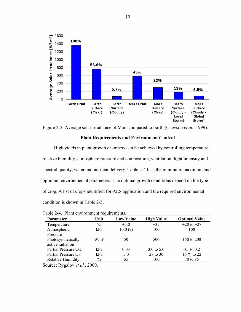
Figure 2-2).
Figure 2-1. Martian spectral irradiance (Ls=250, 15ºS, noon) vs. terrestrial spectral
irradiance (Rettberg et al., 2004)
10
6.5%13%
22%
43%
5.7%
56.6%
100%
0
200
400
600
800
1000
1200
1400
1600
Earth Orbit EarthSurface(Clear)
EarthSurface(Cloudy)
Mars Orbit MarsSurface(Clear)
MarsSurface
(Cloudy -Local
Storm)
MarsSurface
(Cloudy -GlobalStorm)
Ave
rage
Sol
ar I
rrad
ianc
e [W
/m²]
Figure 2-2. Average solar irradiance of Mars compared to Earth (Clawson et al., 1999).
Plant Requirements and Environment Control
High yields in plant growth chambers can be achieved by controlling temperature,
relative humidity, atmosphere pressure and composition, ventilation, light intensity and
spectral quality, water and nutrient delivery. Table 2-4 lists the minimum, maximum and
optimum environmental parameters. The optimal growth conditions depend on the type
of crop. A list of crops identified for ALS application and the required environmental
condition is shown in Table 2-5.
Table 2-4. Plant environment requirements. Parameter Unit Low Value High Value Optimal Value Temperature ºC +5.0 +35 +20 to +27 Atmospheric Pressure
kPa 10.0 (?) 100 100
Photosynthetically active radiation
W/m² 50 500 150 to 200
Partial Pressure CO2 kPa 0.03 3.0 to 5.0 0.1 to 0.2 Partial Pressure O2 kPa 5.0 27 to 30 10(?) to 22 Relative Humidity % 55 100 70 to 85
Source: Rygalov et al., 2000.

11
Table 2-5. Advanced life support crop growth conditions.
Crop
Photo-synthetic
Photon Flux [mol/m²-d]
Diurnal Photoperiod
[h/d]
Growth Period
[days after planting]
Air Temperature
- Day [ºC]
Air Temperature - Night [ºC]
Cabbage 17 85 >25 Carrot 17 75 16-18 Chard 17 16 45 23 23 Celery 17 75 Dry Bean 24 18 85 28 24 Green Onion 17 50 Lettuce 17 16 28 23 23 Onion 17 50 Pea 24 75 Peanut 27 12 104 26 22 Pepper 27 85 Radish 17 16 25 23 23 Red Beet 17 16 38 23 23 Rice 33 12 85 28 24 Snap Bean 24 85 28 24 Soybean 28 12 97 26 22 Spinach 17 16 30 23 23 Strawberry 22 12 85 20 16 Sweet Potato 28 12 85 26 22 Tomato 27 12 85 24 24 Wheat 115 20-24 79 20 20 White Potato 28 12 132 20 16 Source: Hanford, 2004. Temperature
Temperature effect
Temperature is an important physical parameter for controlling plant growth. It has
a direct effect on biochemical reaction rates in the various metabolic processes and can
indirectly contribute to water stress by enhancing transpiration (Downs and Hellmers,
1975). The various biochemical reactions have different minimum, maximum and
optimum temperatures. Up to 30 ºC temperature affects plant growth positively by more
rapid leaf expansion and increased root initiation (Albright et al., 2001). In general, most
plants grow well at a temperature from 10 to 30 ºC. Excessive temperatures result in heat
damage; temperatures below this range lead to chilling and/or freeze damage. The

12
severity of the damage increases with increasing temperature difference and the time the
plant spends in this unfavorable condition.
Temperature control
In order to control the air temperature of a Mars greenhouse, it is essential to
analyze the heat and mass balance of the greenhouse and its environment. Heat received
by the greenhouse through solar radiation or waste heat of internal electric equipment
may lead to a rise of the temperature. Convective, conductive and radiative heat loss of
the greenhouse to the environment may result in a decreasing internal greenhouse
temperature. Furthermore, the addition and removal of latent heat by evaporation and
condensation of water directly affect the plant as well as the greenhouse temperature.
Air temperature can be increased by addition of heat to the greenhouse such as by
turning on the heating system. Temperature is decreased by removing heat from the
greenhouse such as by utilization of cooling coils or maximizing heat emission of the
greenhouse structure to the Mars environment. Temperature uniformity within a
greenhouse is achieved by vertical ventilation.
Relative Humidity
Relative humidity effect
Relative humidity is an indicator of potential water loss from the plants as it is a
function of the water vapor pressure. Transpiration rates of plants increase as the vapor
pressure deficit between the cells of the leaf and the atmosphere increases. At a given
temperature, the vapor pressure deficit increases rapidly with decreasing humidity. The
balance and dynamics of water loss by transpiration and gain by root absorption
determine the plant water status. Water stress and possibly wilting can be caused by a
high transpiration rate and vapor pressure deficit.

13
Humidity also reduces the incident radiation on plants through absorption of
infrared radiation leading to a higher specific heat of the air. Condensation and
evaporation affect the energy balance and therefore the air temperature.
70-85% relative humidity is considered to be the optimal range for plant growth
(Tibbitts, 1979). Low relative humidity levels cause wilting of the plants; high relative
humidity levels lead to development of fungus and mold.
Relative humidity control
In a closed environment, humidity is increased by evaporation of open water
sources or evapo-transpiration of the plants. Humidity levels are reduced by
condensation. Humidity control can be achieved by studying the underlying
psychrometric relationships which are explained in detail in the psychrometrics section at
the end of Chapter 5.
Atmospheric Pressure and Composition
The greenhouse atmosphere is composed of essential gases required for plant
growth (such as carbon dioxide, oxygen and water vapor) and some non-essential gases
(such as nitrogen) for pressurizing the greenhouse structure. The total pressure of the
greenhouse atmosphere is the sum of the partial pressures of the gases.
Carbon dioxide effect
Apart from light and water, carbon dioxide is required for photosynthesis and
therefore plant growth. Plant response to increased/decreased carbon dioxide levels
depends on plant species, development stage, irradiance, temperature and mineral
nutrition (Langhans and Tibbitts, 1997). Slightly elevated carbon dioxide during the day
may lead to increased biomass production, whereas highly elevated carbon dioxide levels
can be toxic for plants. As net photosynthesis increases with elevated carbon dioxide

14
concentration (up to 0.5 kPa), transpiration may decrease due to stomatal closure and leaf
temperatures could rise (Wheeler, 2000). Thus, benefits from elevated carbon dioxide
concentrations can be reduced by higher leaf temperatures. On the other hand, studies
showed that at super-elevated levels of carbon dioxide concentration (0.5-1.0kPa) leaf
transpiration and plant water use increased significantly for some species (Wheeler,
2000). Plant photosynthesis and hence growth responses to carbon dioxide generally
show near linear increases at the low concentrations (up to 0.15 kPa), after which rates
either saturate or eventually taper off. Carbon dioxide concentration below terrestrial
ambient levels (370 ppm) decreases photosynthesis and plant growth (Langhans and
Tibbitts, 1997).
Carbon dioxide control
If carbon dioxide is not controlled in a plant growth chamber, it will decrease
during the day when it is used for photosynthesis. During the night the amount of carbon
dioxide increases due to plant respiration. Carbon dioxide that is taken up by the plants
for photosynthesis has to be replenished to the greenhouse atmosphere. In case of an
autonomous greenhouse, pre-deployed before human arrival, carbon dioxide is not
available as a byproduct of the human metabolism and should be taken out of the carbon
dioxide rich Mars atmosphere.
Oxygen effect
Oxygen is important for respiration, especially at night when there is no
photosynthetically generated oxygen. Probably at least 5 kPa of oxygen is needed to
sustain plant growth (Quebedeaux and Hardy, 1973). Partial pressure of oxygen is
especially critical for the root-zone respiration. The upper limit of oxygen partial pressure
15
can be set at 23.5%, because above this there are safety concerns related to fire risks
(Lacey et al., 2000).
Oxygen control
Photosynthesis produces oxygen and therefore the oxygen levels will build up in a
greenhouse over time. Thus, oxygen has to be scrubbed out of the atmosphere or used by
humans in order to keep the oxygen level constant.
Vapor pressure effect and control
The effect and control of relative humidity have been described above. Under Earth
atmospheric pressure in an open system, the change in vapor pressure has minimal effect
on total pressure, but in a totally closed system at low pressure, fluctuations in vapor
pressure will significantly influence total pressure (Bucklin et al., 2004). This effect is
explained in detail in the psychrometrics section in Chapter 5.
Pressurizing gas
Nitrogen and argon are two inert gases that may be used as pressurizing gases. In
case of a Mars greenhouse both of the gases could be used, as they are available in the
Mars atmosphere, so they could be extracted locally. Nitrogen and argon are biologically
inert. They would be used as make-up gases in order to increase the total pressure
required for the inflatable structure.
Ventilation
The ventilation system ensures a homogenous gas mix in terms of gas composition,
temperature and humidity inside of the greenhouse. Furthermore, ventilation provides a
minimum air velocity over the plants to facilitate gas exchange required for
photosynthesis. On the other hand, excessive air movement through the crop canopy
leads to increased transpiration and potential water stress (Albright et al., 2001).

16
Radiation
Radiation effects
Electromagnetic radiation is the energy source for plant growth. Radiation controls
photosynthesis not only through the intensity but also through the spectral distribution
and photoperiod.
For photosynthesis, plants require photosynthetically active radiation in the
wavelengths between 400 and 700 nm. Photosynthetic efficiency decreases in the region
of 500 to 600 nm where radiation is not absorbed well by the chlorophyll, giving the
plants their characteristic green appearance (see Figure 2-3).
Figure 2-3. Photosynthetic efficiency (Eckart, 1996).
The radiation intensity required to saturate C-3 plants is around 300 µmol/m²-s for
a daily photoperiod of 16 hours; C-4 plants require at least 500 µmol/m²-s for a daily
photoperiod of 16 hours (Langhans and Tibbitts, 1997).
Shade leaves tend to be larger, thinner, and contain more chlorophyll per unit
weight than do sun, i.e., bright light-grown leaves (Boardman, 1977). But sun leaves have
higher photosynthetic capacities. As a consequence, low levels of photosynthetically
active radiation result in bigger leaves, elongation of internodes and less dry weight,

17
whereas high light levels lead to stimulation of auxiliary branch growth and possibly to
photodestruction of chlorophyll. Excess radiation may cause heating of the leaves and
desiccation due to water loss (Langhans and Tibbitts, 1997).
Radiation control
Shading can lower radiation intensity and filters can change the spectrum. On Mars
the low levels of solar radiation may have to be supplemented by light collection systems
or by electric light. Options for electric lights suitable for plant growth are: Incandescent
lamps, fluorescent lamps, high-intensity discharge lamps (e.g. metal halide lamps, high
pressure sodium lamps), xenon lamps and light emitting diodes.
Incandescent light is blackbody radiation as it is created by a heated body. The
spectrum depends on the temperature of the heated element. Most of the energy from
incandescent lights is in the infrared-region. The infra-red radiation is not useful for
photosynthesis and must be dissipated from the growth chamber. The spectrum can be
shifted by changing the voltage to the lamp; the higher the voltage the lower the ratio of
infra-red to visible radiation. Another method of altering the spectrum is the use of filters.
Wavelengths not useful for photosynthesis can be filtered out. The disadvantage of this
method is that the overall radiation is reduced. Incandescent lamps have a very low
efficiency, not more than 10% of the output radiation is within the visible wavelengths
(Langhans and Tibbitts, 1997).
Fluorescent Lamps have many advantages over incandescent lamps. The radiation
output is continuous, generally uniform and the photosynthetically active radiation is
high. Their optimal operation temperature is only about 38° C. In order to alter the
spectrum of the fluorescent lamps the inner wall of the tubes, which emits the radiation,
can be coated with different phosphors. Most fluorescent plant growth lamps are coated

18
with a special phosphor mix to provide an enhanced blue and red spectrum. Cool white
lamps are the most efficient fluorescent lamps, with efficiencies of around 20%. Output
of very high output lamps decreases to 70% after the lamps have been operated for 1
year, 16 hours per day (Langhans and Tibbitts, 1997; Schwarzkopf, 1990).
High-intensity discharge lamps excite elements in the arc in order to emit
characteristic wavelengths. Their spectrum is uniform but not continuous. Irradiances are
higher than those of incandescent and fluorescent lamps. Two commonly used high-
intensity discharge lamps are metal halide and high-pressure sodium lights. In contrast to
fluorescent lamps the output radiation of metal halide lamps is not affected by the
ambient temperature. Most of the radiation output is in the 400-700 nm but output can
shift with lamp age. The efficiency of metal halide lamps is around 22%. The radiation
output of high pressure sodium lamps is concentrated in the 550-650 nm range, and very
scarce in the 400-550 nm range. High pressure sodium lights are useful in combination
with alternative lighting options such as metal halide, blue phosphor and cool-white
fluorescent lamps. High pressure sodium lights are very efficient with efficiencies of 25%
(Langhans and Tibbitts, 1997; Schwarzkopf, 1990).
Xenon lamps are rarely used for plant growth chambers even though they have a
spectrum similar to the solar spectrum. Their disadvantages include the high cost and
their emission of ultraviolet radiation, which leads to development of ozone.
Furthermore, the high infra-red radiation increases the cooling load of the plant growth
chamber (Langhans and Tibbitts, 1997).
Light emitting diodes (LEDs) are very useful for plant growth as certain LEDs have
specific outputs required for photosynthesis. Moreover, they are solid state devices and

19
have a long operating life. Blue and red LEDs can be combined to fulfill the plant needs
(Langhans and Tibbitts, 1997).
Growth Area
The size of the Mars greenhouse depends on the number of astronauts and the
desired amount of food grown locally vs. shipped from Earth. The required plant-growth
area per person can be estimated at 50 m² to fulfill 100% of the food requirements
(Wheeler et al., 2001). Food, if grown on-site, can regenerate some or all of the crew’s
air and water. If more than about 25% of the food, by dry mass, is produced locally, all
the required water can be regenerated by the same process. If approximately 50% or more
of the food, by dry mass, is produced on site, all the required air can be regenerated by
the same process depending on the crop and growth conditions (Wheeler et al., 2001;
Hanford, 2004).
Low Pressure Plant Growth Studies
Operating a greenhouse on Mars at low internal pressure reduces the pressure
differential across the structure and therefore saves structural mass as well as reduces
leakage. The literature contains a variety of studies on the plant responses to low
pressure. The lower limits of oxygen, carbon dioxide, water vapor and inert gases that
plants can tolerate and thrive in are a key in the development of hypobaric Mars
greenhouses.
Studies on plant responses to low pressure date back to the 1960s, when NASA
first considered the implementation of biological life support systems. These studies
include research at Brooks Air Force Base where the plant environment pressure was
dropped to 51 and 93 kPa and other research Wright-Patterson Air Force Base with an

20
even lower pressure of 1/3 atmosphere. No adverse effects on plant growth due to low
pressure were observed (Corey et al., 2002).
Further studies focused on the effect of the different atmosphere components on the
seed germination, seedling development and plant growth. Andre and Richaud (1986)
and Andre and Massimino (1992) evaluated if an inert gas such as nitrogen is necessary
for plant growth by studying barley at 7 kPa. They concluded that nitrogen is not
necessary for plant growth. An increased transpiration rate was observed at this low
pressure. Furthermore, these studies demonstrated that growth of wheat is possible at a
total pressure as low as 10 kPa. Wheat growth at 20 kPa was greater than at 10 kPa and
even greater than at atmospheric pressure levels.
Musgrave at al. (1988) found enhanced growth of mungbean at 21-24 kPa total
pressure atmospheres with a low oxygen level of 5kPa. A study by Schwartzkopf and
Mancinelli (1991) confirmed that an oxygen partial pressure of at least 5 kPa is necessary
for seed germination and initial plant growth, as seeds failed to germinate at atmospheres
with a partial pressure of oxygen lower than 5 kPa. With a total pressure of 6 kPa and
therefore an oxygen concentration of 83%, this study was well above the oxygen level of
23.5% that is the upper limit considered to be safe regarding fire hazards (Lacey et al.,
2000). Although others have operated systems at high oxygen concentration, e.g. Goto et
al. (2002) operated the growth chamber at a high level of 91% oxygen (21 kPa partial
oxygen pressure, 23 kPa total pressure).
Spanarkel and Drew (2002) reported that lettuce grown at 70 kPa total pressure was
normal in appearance, and that photosynthesis was unaffected compared to plant growth

21
at ambient pressure. Oxygen levels were maintained at 21 kPa and carbon dioxide at
66.5–73.5 Pa during both ambient and hypobaric conditions.
Research by Daunicht and Brinkjans (1996) compared plant growth at 100 kPa to
70 kPa and 40 kPa total pressure with equal carbon dioxide concentration. Photosynthetic
rate increased at 70 kPa compared to 100 kPa and was similar at 40 kPa and 100 kPa.
Furthermore, plant morphology was affected by the reduced pressures.
Experiments conducted in the variable pressure growth chambers at different
NASA centers tested wheat under 70 kPa and lettuce under a progressive reduction of
pressure down to 20 kPa (Corey et al., 1996; Corey et al., 1997b, Corey et al., 2002).
Lettuce, as well as the wheat experienced increased transpiration at reduced total
pressures. An effect of the oxygen partial pressure on the photosynthesis was also
observed. Photosynthesis increased with decreasing oxygen partial pressure and
decreased if oxygen was injected into the chamber.
Studies at Texas A&M also tested the performance of wheat and lettuce at low
pressures ranging from 30 to 101 kPa (He et al., 2003). Low pressure increased plant
growth and did not alter germination rate. Low oxygen concentration inhibited ethylene
production of lettuce. Low total pressure inhibited ethylene production of wheat, whereas
oxygen reduction did not have an influence on ethylene production for wheat.
The University of Tokyo performed a series of studies on spinach and maize in a
reduced pressure plant growth chamber (Goto et al., 1996; Iwabuchi et al., 1996;
Iwabuchi and Kurata, 2003). Similar to the other studies described above, they observed
increased photosynthesis and transpiration rates at reduced pressures. Furthermore,
stomatal size and aperture of leaves were significantly smaller at reduced total pressures.

22
Ferl et al. (2002) describes the adaptation and plant responses to low pressure
environments. Plant stress includes hypoxic stress, drought stress and heat shock that may
alter plant morphology. For this research genes were analyzed to understand the
fundamental processes that involve gene responses to environmental signals. Genetic
engineering will lead to plants that can tolerate and thrive in extreme environments.
In a study by Wilkerson (2005) evapo-transpiration rates of radishes increased
significantly at a low atmospheric pressure of 12 kPa and a carbon dioxide partial
pressure of 40 Pa. Furthermore, this research concluded that increasing the carbon
dioxide partial pressure from 40 Pa to 150 Pa is an effective countermeasure to wilting of
the plants at low atmospheric pressures because the stomata close at higher carbon
dioxide concentrations and therefore transpiration rates decrease.
The studies described above indicate that plant growth is possible under low
atmospheric pressure. Nevertheless, more detailed research is necessary on the response
of plants to the environment properties especially for more than one life cycle.
Additionally, studies on plant growth chambers exposed to the Martian environmental
conditions are necessary in case of transparent greenhouse structures, as the local climate
has a huge effect on the plant growth conditions. Operating a greenhouse in the Mars
environment may lead to stratification of temperature and humidity, condensation
resulting in lower light levels, as well as degradation of transparent greenhouse materials
leading to a change of the spectrum of the photosynthetically active radiation. Last but
not least, genetic engineering will play an important role in the selection of the crop
suited for advanced life support.

23
CHAPTER 3 OBJECTIVES OF THIS STUDY
This study can be divided into the theoretical (mathematical) simulation and the
experimental work.
The objectives of the experimental part were
• Design of simulated Mars environment and low pressure greenhouse for plant growth.
• Development of control-algorithm to maintain total pressure and temperature of vacuum chamber (simulated Mars environment).
• Development of control-algorithm to maintain total pressure, temperature and gas composition (CO2, O2 and N2 concentration) of greenhouse dome.
• Monitoring of stratification of temperature and relative humidity in greenhouse dome.
• Monitoring of condensation pattern on interior of greenhouse dome and its effect on light reduction.
• Monitoring of plant evapo-transpiration in low pressure greenhouse that is exposed to low temperature environment.
The objectives of the simulation were
• Development of low pressure psychrometric relationships for closed systems and non-standard atmospheres.
• Prediction of temperatures of greenhouse atmosphere, greenhouse floor, interior and exterior greenhouse shell by creating a mathematical model to simulate the heat and mass transfer.
• Prediction of occurrence of condensation on interior of greenhouse dome.
• Comparison of theoretical and experimental results to deduce conclusions.

24
CHAPTER 4 EXPERIMENTAL WORK
System Description
A careful selection of equipment for the set-up of the experimental work was
required in order to fulfill the objectives listed in Chapter 3. A polycarbonate
hemispherical dome with a diameter of 1 meter served as the Mars greenhouse (see
Figure 4-1). The dome was clamped to a re-inforced aluminum base with the help of a
silicon rubber gasket to ensure the enclosure of the system. A 10 centimeter thick layer of
polyurethane foam was fixed to the bottom of the aluminum dome base for insulation.
Feed-throughs in the dome base were used for data transfer, power and gas supply. The
maximum pressure differential that the dome structure could withstand without failure
was estimated to be ±50 kPa. The structural analysis of the dome and its base plate is
presented in Appendix A.
A dome similar to the one that was utilized as a greenhouse model for this study
had been used at NASA’s Kennedy Space Center as an autonomous low pressure growth
chamber. In a preliminary test lettuce was grown at a pressure of 25 kPa for 45 days
(Fowler et al., 2002; Bucklin et al., 2004). However, during this lettuce growth
experiment at NASA the dome was not exposed to simulated Mars conditions as in the
experiments described in this document.
A large stainless steel vacuum chamber was used to simulate the Mars atmosphere
of 0.6 kPa. Its interior volume was comprised by an area of 1.2 meter by 1.2 meter with a

25
height of 1 meter. The chamber was custom-made by Chicago Wilcox based on the
following requirements:
• The vessel should be able to hold a pressure of 0.1 kPa with no significant leakage. • It should be big enough for the greenhouse dome (0.5 m radius) to fit in. • It should have a window on top to allow growth light to penetrate into the chamber. • It should have 12 ports on the side for data transfer, power and gas supply. • It should have a door to move equipment in and out.
The stainless steel chamber was braced on the bottom and on all sides (except for
door) to avoid deflection of the walls because of the huge pressure difference. A 1.27 cm
thick polycarbonate sheet served as a window pane. A grid of steel bars supported the
polycarbonate window (see Figure 4-2).
An industrial freezer shown in Figure 4-3 ensured the low temperature of the
vacuum chamber (simulated Mars environment). The interior temperature of the freezer
could be dropped down to as low as –34 ºC. Initially, jacketing the vacuum chamber with
a heat exchanger was discussed as an option to reduce the temperature inside of the
chamber, but putting the entire vacuum chamber in a freezer had the advantage that the
temperature distribution was more uniform, especially at the chamber window.
A) B) Figure 4-1. Dome used to protect plants from the simulated low pressure, low
temperature Mars environment. A) Empty dome. B) Dome with sensors, scales and flasks installed.

26
Figure 4-2. Vacuum chamber used to simulate the low pressure Mars environment (less than 1% of Earth’s atmosphere).
Figure 4-3. Industrial walk-in freezer ensures low temperature of the vacuum chamber (simulated Mars environment).

27
Two vacuum pumps were installed outside the freezer. A powerful two-stage rotary
vane vacuum pump (DUO 10, Pfeiffer Vacuum) with a volumetric flow rate of
10 m³/hour was connected to the vacuum chamber; a two-stage vacuum pump (DV-85N,
J/B Industries) with a volumetric displacement of 5 m³/hour was connected to the
greenhouse dome. During the experiments the pumps were always turned on and the air
flow was controlled by two solenoid valves that were installed between the pumps and
the chamber/dome. Three mass flow controllers ensured the correct gas mixture that was
fed into the greenhouse dome. The mass flow controllers were connected to bottles of
nitrogen, oxygen and carbon dioxide.
Scale 1 was located on the bottom of the greenhouse. It measured the amount of
water that ran off the greenhouse shell and the recollection funnel. Four scales (Scale 2 to
Scale 5) were installed in the upper part of the dome. They measured the amount of water
that the plants evaporated and transpired. Two flasks, each containing one lettuce plant,
were placed on each of these four scales, leading to a total number of 8 flasks. A
512W/110V cooking range coil was placed in the center of the greenhouse dome and
served as the heater. A 24V fan ensured mixing of the air and minimized temperature, gas
composition and relative humidity stratification.
A high pressure sodium growth light (1000W HPS, Hortilux) was installed above
the vacuum chamber. Two I/O boards, one for data acquisition and one for control, were
connected to the sensors and actuators. They were connected to the computer for
programming and as user interface. Figure 4-4 gives an overview of the experimental
setup.

28
Figure 4-4. Schematic of experimental setup.
Instrumentation and Sensor Calibration
Most commercially available sensors for the measurement of environmental
parameters contain a data sheet with calibration information under standard atmospheric
conditions. However, in this project, the pressure and gas composition of the environment
that the sensors were exposed to differed significantly from the standard atmosphere.
Therefore, the sensors were carefully selected according to the environmental conditions
and a re-calibration of the sensors was performed against a standard sensor that was not
affected by pressure or gas composition.
DS18B20 (Dallas Semiconductor) digital thermometers were selected for
temperature measurements. They were shielded to avoid measurement errors caused by
direct radiation onto the sensors. Relative humidity (RH) was monitored by HIH-3602-L
(Honeywell) capacitance type sensors capable of measuring RH in the range of 0-100%

29
(non-condensing). LI-COR’s LI-190 SA quantum sensor monitored the level of
photosynthetically active radiation inside the greenhouse dome. The carbon dioxide
concentration was measured by Vaisala’s infrared GMP 221 sensor, oxygen
concentration by Maxtec’s Max 250 galvanic cell type sensor. The mass of the
recollected water and the masses of the individual plants were measured by Vishay
Celetron’s LPS-2 kg load cells. Table 4-1 lists the environmental parameters that were
monitored and their corresponding sensors.
Table 4-1. Sensors used to measure environmental parameters, the sensor ranges and accuracies.
Parameter Type Range Accuracy
Temperature DS18B20 digital thermometer (Dallas Semiconductor) -55 to +125 ºC ± 0.5 ºC
Relative Humidity HIH-3602-L capacitance type RH sensor (Honeywell) 0 to 100% ±2%
Light LI-190SA quantum sensor (LI-COR Inc.)
0 to 10,000 µmol/m2/s ±5%
Pressure ASCX15AN (Sensym ICT) 0 to 15 psi ±0.5%
Carbon Dioxide GMP 221 (VAISALA) 0 to 10 % 0.02%
Oxygen Max 250 (MaxTec) 0 to 100% ± 1.0 %
Water / Plant Mass LPS-2 kg Load Cell (Vishay Celtron) 0 to 2 kg ± 0.1 g
A transparent acrylic cylinder with an aluminum base served as calibration
chamber for the sensors. It had an interior diameter of 20.32 cm, a wall thickness of
0.64 cm and a height of 30.48 cm. The cylinder was supported by an aluminum base
containing feed-throughs for data transfer, power and gas supply. An O-ring minimized

30
leakage of air into the cylinder. The structural analysis of the cylinder is presented in
Appendix A. The calibration data of all sensors is found in Appendix B.
Figure 4-5. Cylinder used for calibration of pressure-sensitive sensors and for initial gas mixing control algorithm development.
The performance of the temperature sensors, light sensor and load cells was
unaffected by changes in total pressure. The sensors affected by low pressure, including
relative humidity (RH), carbon dioxide concentration and oxygen concentration, had to
be calibrated for low pressures. Carbon dioxide and oxygen were calibrated by a method
similar to the one described by Mu (2005).
Rygalov et al. (2002) compared various types of RH sensors under low
atmospheric pressure to RH readings from a chilled mirror/dew point hygrometer that is
unaffected by pressure changes. This study concluded that the dry-bulb/wet-bulb method
was not adequate for low pressures as not enough air mass moves over the sensor. In

31
contrast to this, the readings of the capacitance type RH sensor did not change
significantly at different pressures.
As the accuracy of the relative humidity measurements was of major importance to
the study described in this dissertation, further experiments were conducted to confirm
the independence of the output of the capacitance type RH sensor at different pressures.
The RH values of the capacitance sensors were compared to the output of Vaisala’s
HMP 237 by exposing the sensors to a wide range of humidities and pressures. The
HMP 237 is also a capacitance RH sensor, but especially designed to measure RH and
temperature in both pressurized as well as vacuum chambers. The difference in RH of the
Honeywell sensors from Vaisala’s low pressure RH sensor never exceeded 3%. Thus, the
RH values obtained by the Honeywell RH sensors were not corrected for pressure.
81
82
83
84
85
86
87
88
81 82 83 84 85 86 87 88
Reference Relative Humidity (HMP 237) [%]
Rela
tive
Hum
idity
(C
apac
itanc
e Se
nsor
s RH
1 - R
H5) [
%]
RH1RH2RH3RH4RH5TargetRH conf +3%RH conf -3%
Figure 4-6. Comparison of Honeywell capacitance RH sensors to the HMP 237 reference
RH sensor for pressures of 0 to 25 kPa.

32
Leakage Testing
In low pressure plant growth chambers, involving the measurement of gas
exchange rates and evapo-transpiration, it is important to minimize the leakage and to
account for the occurring leakage by making the necessary corrections (Corey, 1997a).
Leakage is defined as
tPPP
L i 14401000
0 ××−
= (4-1)
where: L = leak rate [% vol/day]
Pi = end pressure [kPa]
Po = initial pressure [kPa]
t = time interval [min]
Leakage of Vacuum Chamber
Initial leak tests of the freshly shipped vacuum chamber, showed very high leak
rates of 2.5 kPa/hour. Due to the high leak rate it was not possible to pump the chamber
down to a pressure lower than 4 kPa. Changing the plastic tubing to copper tubing,
attaching C-clamps to the chamber door, sealing ports additionally with Loctite glue,
utilizing high vacuum rated Swaglok valves and installing a powerful new two-stage
rotary vane vacuum pump (DUO 10, Pfeiffer Vacuum) with a volumetric flow rate of
10 m³/hour, led to a reduction of the leakage to 1.65 kPa/hour. Even at this lower leakage
the target Mars equivalent pressure of 0.6 kPa could not be reached in the chamber.
Further leak tests utilizing helium gas and a helium gas detector revealed that the gas was
mainly leaking through the chamber window. Therefore, the window was taken off and a
second layer of gasket was cut out and installed, so that the polycarbonate window would

33
be sandwiched in between the two gaskets. Thus, the window could deflect more, without
causing gaps for the gas to leak in.
Figure 4-7 depicts the strong forces that act upon the window when the chamber is
at low pressure: Photo A depicts the bulging of the polycarbonate window at low
pressures; in Photo B the window gasket is drawn inside by the large pressure difference.
Additionally, vacuum grease was applied to the window and the door. Finding the right
amount of vacuum grease is the key to success: enough to fill the gaps and reduce the gas
leakage but not so much, that lack of friction causes the gasket to dislocate. Finally, a
pressure of 0.07 kPa was achieved, well below the required pressure of 0.6 kPa.
A) Figure 4-7. Forces on chamber window. A) Vacuum chamber at 0.6 kPa with top window
bulging in. B) Gasket drawn into the chamber due to pressure difference.

34
B) Figure 4-7. continued Leakage of Greenhouse Dome
The greenhouse dome was installed in the 0.6 kPa vacuum chamber. Therefore, gas
leaked from the dome into the vacuum chamber, causing the dome pressure to drop. This
leakage was minimized by applying vacuum grease on the dome gasket, tightening the
36 screws of the dome and sealing the feed-throughs with additional glue.
Figure 4-8 presents the data of a combined leak test of the vacuum chamber and the
greenhouse dome. The dome leakage was found to be -0.375 kPa/hour (45 vol%/day) at
20 kPa; the chamber leakage 0.243kPa/hour (972 vol%/day) at 0.6 kPa. Figure 4-4
compares the leak rates of the vacuum chamber/greenhouse dome to other low pressure
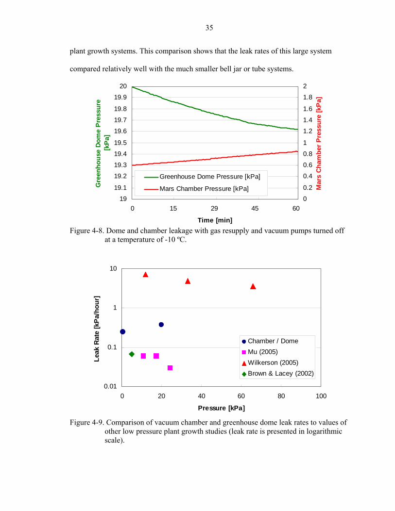
35
plant growth systems. This comparison shows that the leak rates of this large system
compared relatively well with the much smaller bell jar or tube systems.
19
19.1
19.2
19.3
19.4
19.5
19.6
19.7
19.8
19.9
20
0 15 29 45 60
Time [min]
Gre
enho
use
Dom
e Pr
essu
re
[kPa
]
0
0.2
0.4
0.6
0.8
1
1.2
1.4
1.6
1.8
2
Mar
s C
ham
ber P
ress
ure
[kPa
]
Greenhouse Dome Pressure [kPa]
Mars Chamber Pressure [kPa]
Figure 4-8. Dome and chamber leakage with gas resupply and vacuum pumps turned off
at a temperature of -10 ºC.
0.01
0.1
1
10
0 20 40 60 80 100
Pressure [kPa]
Leak
Rat
e [k
Pa/h
our]
Chamber / DomeMu (2005)Wilkerson (2005)Brown & Lacey (2002)
Figure 4-9. Comparison of vacuum chamber and greenhouse dome leak rates to values of
other low pressure plant growth studies (leak rate is presented in logarithmic scale).

36
Data Acquisition and Control System
The distributed control system for this project was developed by Rigel Corporation,
especially for low pressure plant growth experiments, with the aims of maximizing the
inputs and outputs while being very flexible yet low cost. This control system, described
in detail in Mu (2005), was modified and adapted after it had been used for previous plant
growth studies. Two control boards were utilized: one for data acquisition and a second
one to execute the control signals. The two boards combined had a large number of
analog and digital inputs/outputs
• 16 digital inputs for temperature sensors • 16 analog inputs especially for thermocouples • 32 single ended (16 differential) analog inputs • 32 digital outputs for operating the relays • 16 analog outputs for the control of the actuators (such as mass flow controllers) • 8 digital outputs designed for pulse width modulation (e.g. utilized for the control
of the heating system)
The data board and the control board were both connected to the PC via the serial
port. The data acquisition and control software was separated into two parts: The low-
level programming of the microcontrollers was done by Rigel Corporation utilizing
Assembly and C language. These low-level programs, loaded onto the microcontrollers,
received the data from the sensors and sent out control commands to the actuators. For
the high-level programming LabView was chosen as it provides an excellent user-
interface and is comprised of many built-in functions. As LabView is a graphic
programming language it also facilitated multi-users to work with the same program and
to understand it quickly. The LabView programs communicated with the
microcontrollers, contained the control logic and managed the data.

37
Greenhouse Dome Environmental Control
Gas Composition and Total Pressure Control Algorithm
The dry atmosphere of the greenhouse was comprised of three gases: oxygen,
carbon dioxide and nitrogen. Oxygen and carbon dioxide are the essential gases required
for photosynthesis and therefore plant growth. Nitrogen was used to fill up the
atmosphere to the desired total pressure as total pressure is defined as the sum of the
partial pressures of all gases. The oxygen and carbon dioxide concentration of the
greenhouse dome were directly measured by sensors. Nitrogen was calculated by
measuring the total pressure and subtracting the partial pressures of oxygen and carbon
dioxide. Three mass flow controllers were utilized to control the resupply of oxygen,
carbon dioxide and nitrogen separately. Resupply of the individual gas was shut off if the
partial pressure of the gas was higher than the set point partial pressure. If the measured
partial pressure of the gas was lower than the set point, gas was resupplied. The required
mass flow of each gas was calculated by determining the mass of the gas to be resupplied
into the greenhouse dome, resulting in the following gas control algorithm:
tgastgasMassgasMass
tgasFlow actualset
∆−
=)(
),()(),(
ρ (4-2)
where: ),( tgasFlow = gas flow rate [m³/s]
air
domesetset TR
VgasPpgasMgasMass
)()()( = = mass of gas required [kg]
air
domeactualactual TR
VtgasPpgasMtgasMass
),()(),( = = actual mass of gas [kg]
M(gas) = Molecular mass of gas [kg/mol]
Ppset(gas) = partial pressure of gas at setpoint [Pa]

38
Ppactual(gas) = actual partial pressure of gas [Pa]
Vdome = volume of dome [m³]
R = universal gas constant [8.3144J/(mol K)]
Tair = air temperature [K]
ρ(gas)= gas density [kg/m³]
∆t = length of control cycle [s]
Total pressure of the greenhouse dome was maintained constant by controlling
oxygen, carbon dioxide and nitrogen pressures separately as described above. Total
pressure of the vacuum chamber was kept constant by controlling a solenoid valve that
was connected to the vacuum pump. If the vacuum chamber pressure was above the
setpoint, gas was pumped out. If it was below the setpoint the pump was stopped.
Figure 4-10 depicts the oxygen and carbon dioxide partial pressures during a test of
the gas mixing control system that lasted 1 hour. Figure 4-11 shows the total pressures of
the vacuum chamber and the greenhouse dome.
0
0.5
1
1.5
2
2.5
3
3.5
4
4.5
5
0 15 30 45 60
Time [min]
Oxy
gen
Par
tial P
ress
ure
[kP
a]
0
0.2
0.4
0.6
0.8
1
1.2
1.4
Carb
on D
ioxi
de P
artia
l Pre
ssur
e [k
Pa]
Oxygen [kPa]Carbon Dioxide [kPa]
Figure 4-10. Gas mixing of dome greenhouse atmosphere without plants (oxygen set
point at 4.0 kPa and carbon dioxide set point at 0.5 kPa).

39
0
0.5
1
1.5
2
2.5
3
3.5
4
4.5
5
0 15 30 45 60
Time [min]
Cha
mbe
r Pre
ssur
e [k
Pa]
15
16
17
18
19
20
21
22
23
24
25
Dom
e Pr
essu
re [k
Pa]
Mars Chamber Pressure [kPa]
Dome Greenhouse Pressure [kPa]
Figure 4-11. Pressure control of vacuum chamber (set point 0.6 kPa) and greenhouse
dome (set points 20 kPa).
Air Temperature Control Algorithm
Maintaining the air temperature in a range where the plants are productive is
essential in the cold Mars environment. Air temperature was kept constant by the heating
coil that was installed in the center of the greenhouse dome at plant level. The heater was
controlled by pulse width modulation with duty cycles of 0%-100%. At 100% the
maximum power output was calculated to be 512.7 W:
WVR
VP 7.5126.23
)110( 22
max =Ω
== (4-3)
where: Pmax = heating power [W]
V = voltage [V]
R = resistance [Ω]
To maintain the air temperature T3 at a certain set point, the required power of the
heating system was calculated by adding the required steady state power (determined in

40
the following section: see equations 4-5 & 4-6) to a proportional control term with a gain
of 1/ T3air,set:
( ))(33
1),3,()( ,,
, tTTT
LightTTPtP setairsetair
setairfreezerssreq −+= (4-4)
where: Preq(t) = required heating power [W]
Pss(Tfreezer, T3air,set, Light) = steady state heating power [W]
T3air,set = air set point temperature [ºC]
T3air(t) = actual air temperature T3 [ºC]
Figure 4-12 gives an example of how the temperature control algorithm regulated
the air temperature. A constant air temperature of 20 ºC was maintained by varying the
heating power. When the light was turned on the required heating power was much less
than when the light was turned off.
0
5
10
15
20
25
0 60 120 181Time [min]
Air
Tem
pera
ture
T3
[ºC]
0
50
100
150
200
250
300
Hea
ting
Pow
er [W
]
Light on Light offLight off
Figure 4-12. Air temperature control of greenhouse dome (set point at 20 ºC).
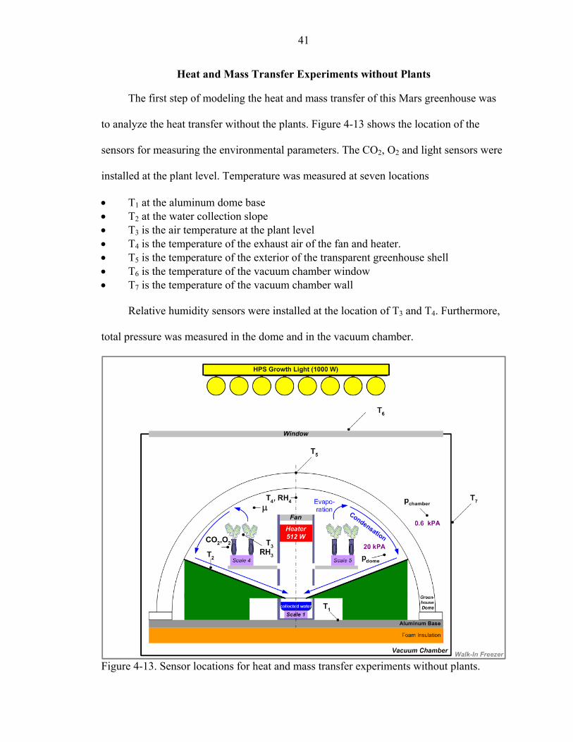
41
Heat and Mass Transfer Experiments without Plants
The first step of modeling the heat and mass transfer of this Mars greenhouse was
to analyze the heat transfer without the plants. Figure 4-13 shows the location of the
sensors for measuring the environmental parameters. The CO2, O2 and light sensors were
installed at the plant level. Temperature was measured at seven locations
• T1 at the aluminum dome base • T2 at the water collection slope • T3 is the air temperature at the plant level • T4 is the temperature of the exhaust air of the fan and heater. • T5 is the temperature of the exterior of the transparent greenhouse shell • T6 is the temperature of the vacuum chamber window • T7 is the temperature of the vacuum chamber wall
Relative humidity sensors were installed at the location of T3 and T4. Furthermore,
total pressure was measured in the dome and in the vacuum chamber.
Figure 4-13. Sensor locations for heat and mass transfer experiments without plants.

42
A) B)
C) D) Figure 4-14. Preparation of the steady state experiments. A) Bottom of dome base with
foam insulation. B) Side view of greenhouse dome with the sensors and scales installed. C) Top view of greenhouse dome without shell. D) Installation of greenhouse dome into the vacuum chamber.
An exact understanding of the temperature distribution at the different locations
illustrated in Figure 4-13 was important to calculate the thermal resistances in Chapter 5.
The greenhouse dome was subjected to a combination of different freezer temperatures,
heating power levels and growth light states:
• Freezer temperatures at 0 ºC, -10 ºC and -20 ºC. • Heating power levels at 0 W, 26 W, 51 W, 77 W and 103 W. • Growth light switched on/off.
Useless combinations such as a heating power of 0W and the growth light switched
off were left out, as well as combinations that resulted in very high dome temperatures

43
(e.g. 0 ºC freezer temperature, 103 W heating power and growth light switched on).
Figure 4-15 depicts the trend of the seven different temperatures for a freezer temperature
of 0 ºC, a heating power of 26 W and the growth light switched off. Temperature T6 at
the window and temperature T7 at the chamber wall oscillated as the freezer temperature
was controlled at 0 ºC within a band of +1 ºC and -1 ºC. The time required to achieve
steady-state temperatures was always at least 10 to 12 hours. The steady state
temperatures at the seven locations for the different combination of freezer temperatures,
heating power levels and growth light state are given in table 4-2. Each experiment was
conducted two times to minimize errors. Figures 4-16 to 4-20 depict the temperature
distributions. It can be observed that the temperatures inside the dome increase linearly
with the increased in heating power. The chamber window (T6) and wall (T7)
temperatures increased only slightly with increasing heating power. On the other hand, T6
and T7 increased significantly when the growth light was turned on.
0
2
4
6
8
10
12
14
16
0 100 200 300 400 500 600Time [min]
Tem
pera
ture
[ºC]
T1 - BaseT2 - SlopeT3 - Air/PlantT4 - Fan ExhaustT5 - Outside ShellT6 - WindowT7 - Wall
Figure 4-15. Temperature readings until steady state is achieved. (0 ºC freezer
temperature, 26 W heating power and light switched off).

44
Table 4-2. Steady state temperature distribution under different freezer temperature, light and heating power conditions.
Freezer Temp.
[ºC]
Lights (0=off, 1=on)
Heating Power
[W]
Base T1
[ºC]
Slope T2
[ºC]
Air/ Plant
T3 [ºC]
Fan Exhaust T4 [ºC]
Shell Outside T5 [ºC]
Window Outside T6 [ºC]
Wall Outside T7 [ºC]
0 0 26 4.34 10.35 12.74 13.72 10.43 0.90 0.01 0 0 51 5.96 15.29 19.17 20.75 15.68 1.83 0.34 0 0 77 6.98 18.93 24.06 26.11 19.69 2.28 0.49 0 0 103 8.56 24.09 30.25 32.60 24.49 2.39 0.11
-10 0 26 -3.44 2.68 5.29 6.38 2.81 -7.56 -9.63 -10 0 51 -3.06 6.61 10.76 12.40 7.17 -8.00 -9.94 -10 0 77 0.34 12.95 18.44 20.59 13.51 -7.00 -9.44 -10 0 103 2.84 17.73 24.01 26.61 17.96 -6.44 -9.38 -20 0 51 -10.81 -0.94 3.38 4.94 -0.03 -17.25 -19.13 -20 0 77 -10.31 3.44 9.06 11.12 4.29 -17.06 -19.31 -20 0 103 -7.19 9.32 15.51 17.96 9.60 -15.94 -18.88 -20 0 128 -4.13 14.39 21.34 24.32 14.14 -15.00 -18.63 -10 1 0 9.47 18.74 16.76 18.96 19.88 8.74 -6.22 -10 1 26 10.12 23.66 25.74 27.08 25.22 9.28 -6.74 -10 1 51 10.61 28.59 32.17 34.15 30.62 9.81 -6.66 -10 1 77 11.96 32.50 38.27 39.56 34.63 10.56 -6.31 -20 1 0 -5.06 6.13 5.60 6.09 7.73 -5.56 -15.38 -20 1 26 1.75 15.37 17.52 18.18 16.76 -5.25 -14.38 -20 1 51 5.09 19.88 23.39 24.48 20.88 -5.06 -14.13 -20 1 77 9.81 27.22 32.73 34.95 29.17 -3.08 -13.85 -20 1 103 11.63 31.73 38.98 41.22 33.68 -3.88 -13.20
0 ºC Freezer Temperature - Light off
0
5
10
15
20
25
30
35
0 50 100 150 200Heating Power [W]
Stea
dy S
tate
Tem
pera
ture
[ºC]
T1 - BaseT2 - SlopeT3 - Air/PlantT4 - Fan ExhaustT5 - Outside ShellT6 - WindowT7 - Wall
Figure 4-16. Steady state temperatures versus power of heater at seven different locations (T1-T7). Freezer temperature is 0 ºC and the growth light is switched off.

45
-10 ºC Freezer Temperature - Light off
-10
-5
0
5
10
15
20
25
30
0 50 100 150 200
Heating Power [W]
Stea
dy S
tate
Tem
pera
ture
[ºC
] T1 - BaseT2 - SlopeT3 - Air/PlantT4 - Fan ExhaustT5 - Outside ShellT6 - WindowT7 - Wall
Figure 4-17. Steady state temperatures versus power of heater at seven different locations (T1-T7). Freezer temperature is -10 ºC and the growth light is switched off.
-20 ºC Freezer Temperature - Light off
-20
-15
-10
-5
0
5
10
15
20
25
30
0 50 100 150 200Heating Power [W]
Stea
dy S
tate
Tem
pera
ture
[ºC
]
T1 - BaseT2 - SlopeT3 - Air/PlantT4- Fan ExhaustT5 - Outside ShellT6 - WindowT7 - Wall
Figure 4-18. Steady state temperatures versus power of heater at seven different locations (T1-T7). Freezer temperature is -20 ºC and the growth light is switched off.

46
-10 ºC Freezer Temperature - Light on
-10
-5
0
5
10
15
20
25
30
35
40
0 50 100 150 200Heating Power [W]
Ste
ady
Stat
e Te
mpe
ratu
re [º
C]
T1 - BaseT2 - SlopeT3 - Air/PlantT4 - Fan ExhaustT5 - Outside ShellT6 - WindowT7 - Wall
Figure 4-19. Steady state temperatures versus power of heater at seven different locations (T1-T7). Freezer temperature is -10 ºC and the growth light is switched on.
-20 ºC Freezer Temperature - Light on
-20
-10
0
10
20
30
40
50
0 50 100 150 200Heating Power [W]
Ste
ady
Sta
te T
empe
ratu
re [º
C]
T1 - BaseT2 - SlopeT3 - Air/PlantT4 - Fan ExhaustT5 - Outside ShellT6 - WindowT7 - Wall
Figure 4-20. Steady state temperatures versus power of heater at seven different locations
(T1-T7). Freezer temperature is -20 ºC and the growth light is switched on.
Figure 4-21 depicts the steady state air temperature T3 of the greenhouse dome for
different heating power and freezer temperatures. The steady state air temperature

47
increases linearly with increasing heater power. The linear equations for the freezer
temperatures of 0 ºC, -10 ºC and -20 ºC are shown in Figure 4-21. According to the
equations, the steady state air temperature is not equal to the freezer temperature when
the heating system is switched off. This difference results from the waste heat that is
introduced by running the fan continuously and the difference of freezer temperature and
wall temperature of the vacuum chamber T7 (see Table 4-2). Combining these three
equations into one, the power of the heater required to heat the air to temperature T3 with
a freezer temperature of Tfreezer can be calculated as follows:
23047.0)000598.0(
741.7)831.0(,3
+×−
+×−=
freezer
freezerair
TTT
Pss (4-5)
where: Pss = power of heater [W]
T3,air = steady state temperature of air T3 [ºC]
Tfreezer = temperature of freezer [ºC]
T3ss(0 ºC) = 0.2240*W + 7.2000R2 = 0.9975
T3ss(-10 ºC) = 0.2490*W - 1.3350R2 = 0.9954
T3ss(-20 ºC) = 0.2353*W - 8.7930R2 = 0.99940
5
10
15
20
25
30
35
0 50 100 150
Heating Power[W]
Stea
dy S
tate
Air
Tem
pera
ture
T3
[ºC] 0 ºC Freezer / Light off
-10 ºC Freezer / Light off
-20 ºC Freezer / Light off
Figure 4-21. Steady state air temperatures (T3) versus power of heater for freezer
temperatures of 0 ºC, -10 ºC and -20 ºC (growth light switched off).

48
When the light is switched on, the power of the heater required to heat the air to
temperature T3 with a freezer temperature of Tfreezer can be calculated as following:
2146.0)00526.0(
27.26)951.0(,3
+×−
+×−=
freezer
freezerair
TTT
Pss (4-6)
Figure 4-22 depicts the heating power requirement depending on the freezer
temperature for steady state air temperatures T3 of 15 ºC, 20 ºC and 25 ºC. When the
growth light was switched off and if the freezer temperature was -20 ºC, e.g., the required
heater power was 95.5 W, 116.2 W and 136.8 W to achieve a steady state air temperature
of 15 ºC, 20 ºC and 25 ºC respectively. If the growth light was switched on, the required
heating power was reduced significantly. At a freezer temperature of -20 ºC and an air
temperature of 20 ºC, the heating power was reduced by 79.8 W, with the light switched
on.
0
50
100
150
200
250
300
350
-40 -35 -30 -25 -20 -15 -10 -5 0
Freezer Temperature [ºC]
Hea
ting
Pow
er [W
]
Air Temperature = 15ºC / light onAir Temperature = 20ºC / light onAir Temperature = 25ºC / light onAir Temperature = 15ºC / light offAir Temperature = 20ºC / light offAir Temperature = 25ºC / light off
∆P(20ºC)= 79.8 W
Figure 4-22. Freezer temperature versus power of heater for steady state air temperatures
(T3) of 15 ºC, 20 ºC and 25 ºC.

49
If the interior temperature of the greenhouse dome shell decreased below the dew
point of the air temperature, condensation could occur. Figure 4-23 shows two photos of
condensation on the inside of the greenhouse dome. High condensation occurred for low
freezer temperatures (Photo B) as those low temperatures resulted in a lower greenhouse
shell temperature. These photos also clearly show a stratification of temperature within
the greenhouse dome. The top of the dome was warmed by radiation of the growth light
and the air from the heating system that the fan blew across the inside shell. As the
greenhouse shell was colder close to the water recollection funnel (black surface)
condensation was more likely to occur there. The bottom of the greenhouse dome near
the aluminum base showed less condensation, because the relative humidity was less in
the lower part of the dome as the flasks were installed in the upper level. The curvature of
the dome shell and the slope of the recollection funnel led to runoff of the water to the
collection container located on scale 1 (see Figure 4-13). Under certain conditions, ice
crystals had been observed on the aluminum base as temperatures may have dropped
below 0ºC, even though the dome base was well insulated.
During the long-term experiments involving lettuce plants (see next section) water
evaporated from the collection container and the relative humidity in the bottom part of
the greenhouse increased. Condensate and frost formed on the lower part of the
greenhouse shell and the dome base plate due to the low temperatures. This can be clearly
observed in the two photos shown in Figure 7-1, which were taken after the vacuum
chamber was opened at the end of the 7 day experiment.
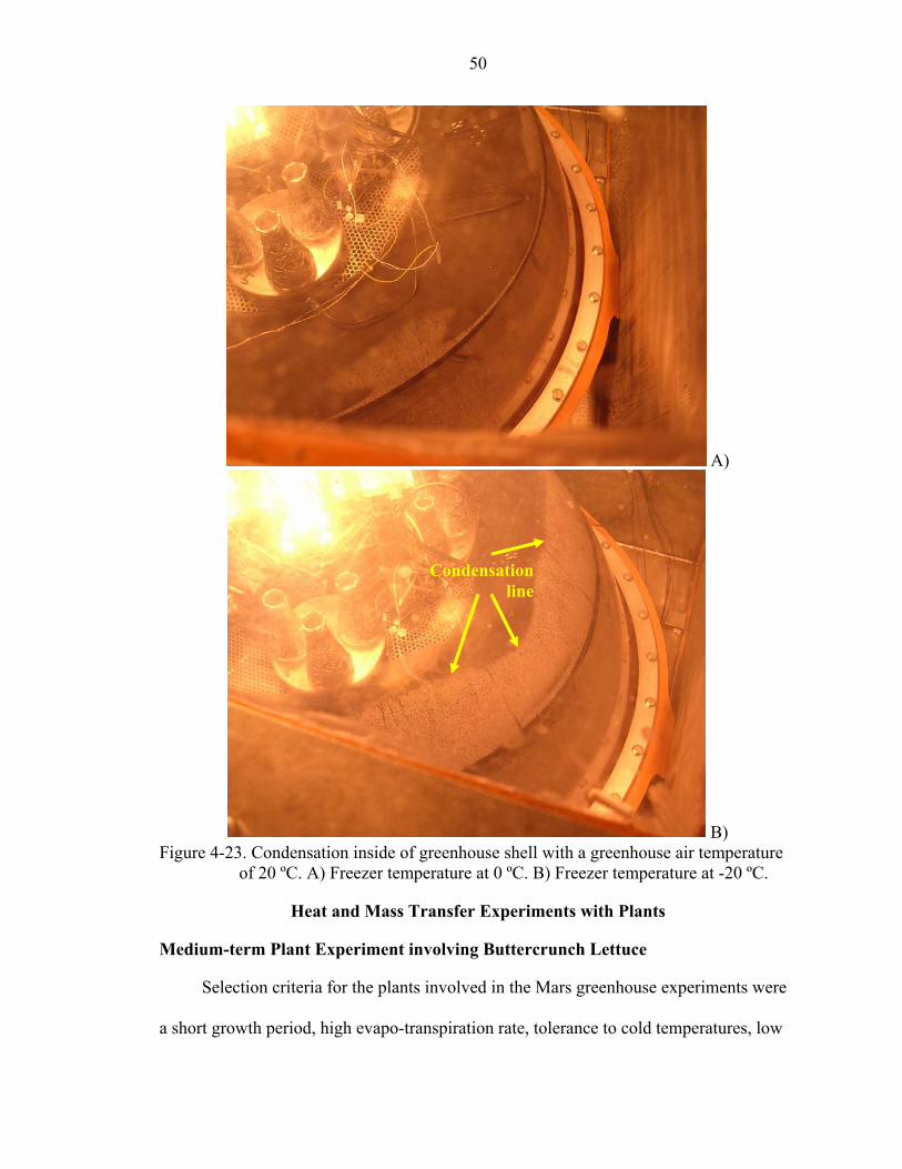
50
A)
B) Figure 4-23. Condensation inside of greenhouse shell with a greenhouse air temperature
of 20 ºC. A) Freezer temperature at 0 ºC. B) Freezer temperature at -20 ºC.
Heat and Mass Transfer Experiments with Plants
Medium-term Plant Experiment involving Buttercrunch Lettuce
Selection criteria for the plants involved in the Mars greenhouse experiments were
a short growth period, high evapo-transpiration rate, tolerance to cold temperatures, low
Condensation line

51
light requirements, suitability for hydroponic growth in 150 ml Ehrlenmeyer flasks and
dome height constraints. Buttercrunch lettuce (Lactuca Sativa cv. Buttercrunch) was
selected as lettuce is one of NASA’s baseline crops (see Chapter 2) and it fulfills the
criteria mentioned above. Six weeks old lettuce plants grown in soil under atmospheric
conditions were transplanted into flasks filled with 50% water and 50% nutrient solution.
The flasks were wrapped in aluminum foil to avoid growth of algae caused by direct
radiation onto the nutrient solution. One hole of the stopper was cut open from the side
and the plant was carefully inserted. Evaporation of the hydroponic solution was avoided
by sealing the gap between the plant and the stopper with putty as shown in Figure 4-24.
Eight flasks were placed into the greenhouse dome; two on each scale (see Figure 4-25).
A) B)
Figure 4-24. Buttercrunch lettuce in Ehrlenmeyer flask. A) The average height of the shoot zone is 15 cm. B) Putty and a stopper prevent evaporation of the hydroponic solution as they separate the root from the shoot zone.

52
Figure 4-25. Installation of flasks containing the lettuce plants onto the scales.
The plants were exposed to a controlled environment inside the greenhouse dome
for 36 hours. The environment conditions and their control methods are summarized in
Table 4-3. The air temperature and the gas composition were tightly controlled by
actuators. A total pressure of 25 kPa was selected as plants still were to be productive at
this low pressure level. The partial pressure of oxygen was set to 4 kPa, resulting in an
oxygen level of 16%, lower than on Earth because oxygen is a very precious resource
during a space mission on Mars: it must be shipped from Earth as it is barely available in
the Mars atmosphere and will be mainly used for human breathing. The partial pressure
of carbon dioxide was set to a high level of 0.8 kPa, as carbon dioxide can easily be
extracted from the Mars atmosphere. High levels of carbon dioxide are known to enhance
plant growth.
The greenhouse humidity was passively controlled by the equilibrium between
evaporation of the water from the plants and the open water surfaces versus the
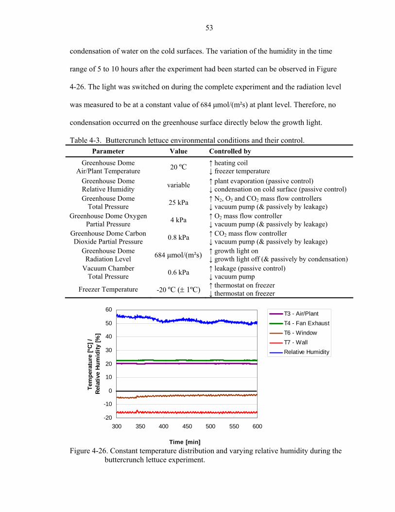
53
condensation of water on the cold surfaces. The variation of the humidity in the time
range of 5 to 10 hours after the experiment had been started can be observed in Figure
4-26. The light was switched on during the complete experiment and the radiation level
was measured to be at a constant value of 684 µmol/(m²s) at plant level. Therefore, no
condensation occurred on the greenhouse surface directly below the growth light.
Table 4-3. Buttercrunch lettuce environmental conditions and their control. Parameter Value Controlled by
Greenhouse Dome Air/Plant Temperature 20 ºC ↑ heating coil
↓ freezer temperature Greenhouse Dome Relative Humidity variable ↑ plant evaporation (passive control)
↓ condensation on cold surface (passive control) Greenhouse Dome
Total Pressure 25 kPa ↑ N2, O2 and CO2 mass flow controllers ↓ vacuum pump (& passively by leakage)
Greenhouse Dome Oxygen Partial Pressure 4 kPa ↑ O2 mass flow controller
↓ vacuum pump (& passively by leakage) Greenhouse Dome Carbon Dioxide Partial Pressure 0.8 kPa ↑ CO2 mass flow controller
↓ vacuum pump (& passively by leakage) Greenhouse Dome
Radiation Level 684 µmol/(m²s) ↑ growth light on ↓ growth light off (& passively by condensation)
Vacuum Chamber Total Pressure 0.6 kPa ↑ leakage (passive control)
↓ vacuum pump
Freezer Temperature -20 ºC (± 1ºC) ↑ thermostat on freezer ↓ thermostat on freezer
-20
-10
0
10
20
30
40
50
60
300 350 400 450 500 550 600
Time [min]
Tem
pera
ture
[ºC
] /
Rel
ativ
e H
umid
ity [%
]
T3 - Air/PlantT4 - Fan ExhaustT6 - WindowT7 - WallRelative Humidity
Figure 4-26. Constant temperature distribution and varying relative humidity during the
buttercrunch lettuce experiment.

54
Figure 4-27 depicts the rates of plant evapo-transpiration from the scales 2-5.
Scale 1 measured the water in the recollection container. It had been filled with
245 grams of water before the experiment in order to keep the humidity high at the
beginning of the experiment. The change of the mass value of scale 1 is the difference
between water evaporating from the open water surface and recollected water dripping
into the container. A positive slope indicates more water was recollected than evaporated,
a negative slope leads to the conclusion that more water was evaporated than re-collected.
Surprisingly, in this experiment the slope of scale 1 had a negative value of –0.0661.
Thus, the recollection system proved to be inefficient as less water was recollected than
had evaporated. This resulted in higher humidities in the lower greenhouse part and
therefore water condensation on the cold dome aluminum base. The plant evapo-
transpiration can be calculated by dividing the water evaporation rate of the scale by the
plant leaf area per scale.
In order to calculate the plant leaf area, the leaves were cut off the plants at the end
of the experiment and the silhouettes were drawn on a white sheet of paper. The
silhouettes were scanned together with a calibration square. The pictures were converted
to black and white images and the silhouettes were filled with black ink. The pictures
were read into matlab and an image processing code determined the ratio of white to
black pixels. The resulting values of the plant leaf areas per scale are given in Table 4-4.
Plant evapo-transpiration varied from 1.6 g/(min m²) to 2.87 g/(min m²). Evapo-
transpiration rates for lettuce under atmospheric conditions are given as 1.23 g/(min m²)
in NASA’s Baseline Values and Assumptions Document (Hanford, 2004). Low pressure
increases evaporation rates and therefore the evapo-transpiration values calculated in the

55
research described in this document seem reasonable. It should be noted that evapo-
transpiration rates are further affected by other factors, including relative humidity, air
temperature, leaf temperature, radiation level and lettuce cultivar, making it difficult to
compare the values of different experiments.
m1 = -0.0661*t + 249.99R2 = 0.8428
m4 = -0.1187*t + 392.48R2 = 0.8827
m2 = -0.1382*t + 379.57R2 = 0.9692
m3 = -0.1308*t + 370.65R2 = 0.9279
m5 = -0.1052*t + 348.2R2 = 0.9003
200
220
240
260
280
300
320
340
360
380
400
300 350 400 450 500 550 600Time [min]
Mas
s [g
]
Scale 1
Scale 2
Scale 3
Scale 4
Scale 5
Figure 4-27. Plant evapo-transpiration rates of plants from 5 to 10 hours after the
beginning of the experiment.
Table 4-4. Evaporation rates per scale with scales 2-5 containing two lettuce plants each. Scale 1 Scale 2 Scale 3 Scale 4 Scale 5
Evaporation/Time [g/min] 0.0661 0.1382 0.1308 0.1187 0.1052 Leaf Area Plant 1 [m²] - 0.042335 0.0234 0.039542 0.032599Leaf Area Plant 2 [m²] - 0.033219 0.02215 0.023296 0.033002Total Leaf Area [m²] 0.075554 0.045549 0.062838 0.065601
Evapo-transpiration Rate[g/min/m²] 1.83 2.87 1.89 1.60
At the end of the experiment, seven out of the eight plants appeared to be healthy
and without visible damage. One plant started wilting after the water level inside the flask

56
decreased to a point where the roots could not reach the remaining water and nutrient
solution (see Figure 4-28).
Figure 4-28. Lettuce plants after an exposure of 36 hours to the controlled Mars greenhouse environment. Healthy plant without any visible physical damage on the left side, wilted plant with roots that do not reach water and nutrient supply on the right side.
Long-term Plant Experiment involving Galactic Lettuce
For the long-term plant experiments Galactic lettuce plants (Lactuca Sativa cv.
Galactic) were selected (see Figure 4-29). The plants were grown from seeds in the
departmental environment-controlled growth chamber under atmospheric conditions with
a day-night cycle of 12 hours. After four weeks, measuring an average height of 8 cm, the
lettuce plants were transplanted into the flasks filled with the hydroponic nutrient
solution. Similar to the previous experiment, eight plants were installed into the
greenhouse dome, two per scale. Table 4-5 lists the environmental conditions the plants
were exposed to and their control. All environmental parameters except of the total dome

57
pressure were kept the same as in the buttercrunch lettuce experiments. The greenhouse
dome total pressure was lowered to 20 kPa.
Figure 4-29. Galactic lettuce plant for long-term experiments with an average height of 8 cm.
Table 4-5. Galactic lettuce environmental conditions and their control. Parameter Value Controlled by
Greenhouse Dome Air/Plant Temperature 20 ºC ↑ heating coil
↓ freezer temperature Greenhouse Dome Relative Humidity variable ↑ plant evaporation (passive control)
↓ condensation on cold surfaces (passive control) Greenhouse Dome
Total Pressure 20 kPa ↑ N2, O2 and CO2 mass flow controllers ↓ vacuum pump (& passively by leakage)
Greenhouse Dome Oxygen Partial Pressure 4 kPa ↑ O2 mass flow controller
↓ vacuum pump (& passively by leakage) Greenhouse Dome Carbon Dioxide Partial Pressure 0.8 kPa ↑ CO2 mass flow controller
↓ vacuum pump (& passively by leakage) Greenhouse Dome
Radiation Level 0 or 684 µmol/(m²s)
↑ growth light on ↓ growth light off (& passively by condensation)
Vacuum Chamber Total Pressure 0.6 kPa ↑ leakage (passive control)
↓ vacuum pump
Freezer Temperature -20 ºC (± 1ºC) ↑ thermostat on freezer ↓ thermostat on freezer

58
Figure 4-30 shows the locations of the sensors for the second set of plant
experiments. Various temperature sensors were added or moved from their previous
position: T2 was moved from the recollection funnel to the inside of the greenhouse dome
shell, T5 was moved to the side of the exterior greenhouse shell, T6 was fixed to the
inside of the vacuum chamber wall, T7 on the outside of the chamber wall at medium
height, T8 at the bottom of the chamber wall and T9 measured the freezer air temperature.
Figure 4-30. Sensor locations for the long-term experiments with galactic lettuce plants.
Plants were exposed to the low pressure controlled greenhouse environment for
7 days. Initially they were exposed to the growth light for 24 hours until steady state of
all parameters was reached, the following days the day-night cycle was set to 12 hours.
Figure 4-31 illustrates the temperature changes over time during the experiment. The air

59
temperature at plant level was controlled at 20 ºC, the freezer temperature was controlled
at -20 ºC (± 1ºC). Figure 4-32 depicts the steady state temperatures during the day and
night cycle, when the growth light was switched on/off, respectively. A heating power of
40 Watts was required to maintain an air temperature of 20 ºC at the plant level during
the day cycle, a heater power of 119 Watts during the night cycle. The temperature of the
fan exhaust was higher for the night cycle as more heating was required, all other
temperatures were lower when the growth light was switched off compared to when the
growth light was switched on.
-30
-20
-10
0
10
20
30
0 24 48 72 96 120 144 168Time [hours]
Tem
pera
ture
[ºC
]
T3 - Air/Plant
T4 - FanExhaust
T2 - InsideShell
T5 - OutsideShell
T6 - ChamberWall Inside
T7- ChamberWall OutsideMiddleT9 - AirFreezer
T8 - ChamberWall OutsideBottom
Light ON
Light ON
Light ON
Light ON
Light ON
Light ON
Light OFF
Light OFF
Light OFF
Light OFF
Light OFF
Light OFF
Light ON
Figure 4-31. Temperature variations during the long-term galactic lettuce experiment.

60
-20-15-10-505
10152025
Air/
Pla
ntTe
mp.
T3
Fan
Exh
aust
Tem
p. T
4
She
ll In
side
Te
mp.
T2
She
ll O
utsi
deTe
mp.
T5
Insi
de W
all
Tem
p. T
6
Out
side
Wal
lM
iddl
e Te
mp.
T7
Out
side
Wal
lB
otto
m T
emp.
T8
Cha
mbe
r Air
Tem
p. T
9
Stea
dy S
tate
Tem
pera
ture
[ºC
] Light off (119 W Heating)Light on (40 W Heating)
Figure 4-32. Comparison of steady state temperature distribution of the day cycle to the
night cycle during the long-term plant experiments.
Figure 4-33 shows the variation of the relative humidity during the day and night
cycle. Before the experiment started, when the greenhouse dome was closed but the
freezer not switched on yet, the relative humidity rose to 70%. This high humidity was
due to addition of water vapor to the atmosphere by plant evapo-transpiration and the
lack of water vapor removal by condensation as the temperatures of the all surfaces of the
greenhouse were at temperatures above 20 ºC and therefore above the dew-point.
Relative humidity decreased to 35% during the first 24 hours when the growth light was
switched on. During the following day-night cycles the relative humidity varied between
a maximum of 35% when the growth light was switched on and a minimum of 28% when
the growth light was switched off. Relative humidity was low during the night cycle as
more condensation occurred due to the lower temperatures of the greenhouse surfaces.

61
Relative humidity was high during the day due to less condensation and more evapo-
transpiration of the plants.
0
10
20
30
40
50
60
70
80
0 24 48 72 96 120 144 168Time [hours]
RH
[%]
Light ON
Light ON
Light ON
Light ON
Light ON
Light ON
Light ON
Light OFF
Light OFF
Light OFF
Light OFF
Light OFF
Light OFF
Figure 4-33. Relative humidity variation during the day and night cycle.
Figure 4-34 shows the effectiveness of the gas composition control, resulting in a
constant gas composition even when all other environmental parameters were subject to
great variations. Changes in temperature, relative humidity and radiation level did not
affect the gas composition of 20 kPa total pressure, 4 kPa oxygen partial pressure and 0.8
kPa carbon dioxide partial pressure.

62
0
2
4
6
8
10
12
14
16
0 24 48 72 96 120 144 168Time [hours]
Dom
e P
artia
l Pre
ssur
es [k
Pa]
N2O2CO2
Figure 4-34. Gas composition control of the greenhouse atmosphere. Set points are
20 kPa for total pressure, 4 kPa for oxygen partial pressure and 0.8 kPa for carbon dioxide partial pressure.
Figure 4-35 shows the mass values of the scales that were measured from 5 to 10 hours
after the galactic lettuce plant experiment had started. For this experiment only two out of
the five scales were connected to the data acquisition system due to the limited amount of
available channels because of the added temperature sensors. The evapo-transpiration
rates of the plants were determined with the same leaf area calculation method described
earlier in this Chapter. The evapo-transpiration rates were found to be 3.71 g/min/m² for
scale 2 and 4.84 g/min/m² for scale 3. These evaporation rates are slightly higher than the
ones in the Buttercrunch lettuce experiments. One possible reason is that the pressure was
reduced from 25 kPa to 20 kPa, leading to an increase in mass diffusivity and therefore
higher evaporation rates.

63
m3 = -0.1132*t + 314.83R2 = 0.9801
m2 = -0.1128*t + 303.16R2 = 0.9572
200
210
220
230
240
250
260
270
280
290
300 360 420 480 540 600Time [min]
Mas
s [g
]
Scale2
Scale3
Figure 4-35. Water evaporation measured on scale 2 and 3 during the galactic lettuce
plant experiment.
Figure 4-36 shows the galactic lettuce plants after they were exposed to the low
pressure Mars greenhouse environment for 7 days. They showed only slight visible
physical damage such as minor signs of water stress (see Figure 4-37 A and B).
Figure 4-36. Galactic lettuce plants after exposure of seven days to the low pressure Mars
greenhouse environment.

64
A)
B) Figure 4-37. Visible damages of the plants. A) and B) Wilting/drying of the plant leaves.

65
CHAPTER 5 MATHEMATICAL MODEL DEVELOPMENT
Effect of Low Pressure on Heat and Mass Transfer
Operating the greenhouse dome at a reduced pressure in the low pressure Mars
environment has a huge influence on the heat and mass transfer. Of the three heat transfer
modes conduction, convection and radiation, convective heat transfer is the one that is
most dependent on the total pressure. Regarding the mass transfer, evaporation rates have
to be analyzed for pressure dependency. Furthermore, the effect of the low pressure on
psychrometric relations should be studied, in order to be able to determine the state of the
moist air.
Convection Heat Transfer
Convection is defined as heat transfer between a surface and a fluid moving over
the surface. Convective heat transfer at low pressures is analyzed based on the equations
given in Incropera and DeWitt (2002). The convection heat transfer depends on the
convection coefficient and on the temperature difference of the moving fluid and the
surface:
)( ∞−=″ TThq s (5-1)
where: q″ = heat flux [W/m²]
h = convection coefficient [W/(m2 K)]
Ts = surface temperature [K]
T∞ = fluid temperature [K]
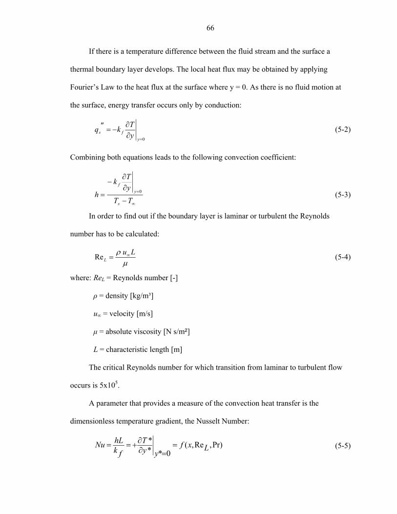
66
If there is a temperature difference between the fluid stream and the surface a
thermal boundary layer develops. The local heat flux may be obtained by applying
Fourier’s Law to the heat flux at the surface where y = 0. As there is no fluid motion at
the surface, energy transfer occurs only by conduction:
0=∂∂
−=″
yfs y
Tkq (5-2)
Combining both equations leads to the following convection coefficient:
∞
=
−
∂∂
−
=TT
yTk
hs
yf
0 (5-3)
In order to find out if the boundary layer is laminar or turbulent the Reynolds
number has to be calculated:
µρ Lu
L∞=Re (5-4)
where: ReL = Reynolds number [-]
ρ = density [kg/m³]
u∞ = velocity [m/s]
µ = absolute viscosity [N s/m²]
L = characteristic length [m]
The critical Reynolds number for which transition from laminar to turbulent flow
occurs is 5x10⁵.
A parameter that provides a measure of the convection heat transfer is the
dimensionless temperature gradient, the Nusselt Number:
Pr),Re,(0**
*Lxf
yyT
fkhLNu =
=∂∂+== (5-5)

67
where: sTT
sTTT
−∞
−=* = dimensionless temperature
Lyy =* = dimensionless variable
The average Nusselt number represents the average heat transfer independent of
location:
Pr),(ReLf
L fk
LhNu == (5-6)
The Prandtl number is the ratio of the properties ν/α:
fkpc µ
αν ==Pr (5-7)
where: ν = dynamic viscosity [m²/s]
α = thermal diffusivity [m²/s]
cp = specific heat [kJ/(kg K)]
kf = conduction coefficient [W/(m K)]
Laminar flow over a horizontal plate
For laminar flow, the Reynolds number has to be below the critical Reynolds
number of 5x10⁵:
5, 105Re ×== ∞
µρ Lu
criticalL (5-8)
For laminar flow the Nusselt number may be obtained from:
6.0Pr3/1Pr2/1Re664.0 ≥== LfkLhLNu (5-9)
Inserting Equations 5-4 and 5-7 into Equation 5-9, results into the following convection
coefficient:

68
6.0Pr2/1
3/2)(3/1)(6/12/1)(664.0 ≥∞=
Lfk
pc)(
uLh
µρ (5-10)
Therefore, convective heat transfer depends on the following parameters: High
density, specific heat and thermal conductivity increase heat transfer. Low absolute
viscosity increases heat transfer.
Specific heat as well as absolute viscosity are independent of density, i.e., pressure.
They are only dependent on temperature. Thermal conductivity is also independent of the
air pressure. Thus, the convection transfer coefficient decreases with the square root of
density/pressure.
2/1)(~ pressurehL for )(~ constTpressuredensity = (5-11)
Thus, the convection coefficient of a gas at a pressure of 20 kPa is 44.7 % of the
convection coefficient of gas at a pressure of 100 kPa for laminar fluid flow with same
velocity and temperature:
)100(447.0)100(10020)20(
2/1
kPahkPahkPah LLL =×⎟⎠⎞
⎜⎝⎛= (5-12)
Turbulent flow over a horizontal plate
For turbulent flow, the Reynolds number has to be above the critical Reynolds
number of 5x10⁵. For turbulent flow the Nusselt number may be obtained from:
3/15/4 PrRe037.0 Lf
LLk
LhNu == (5-13)
Inserting the Reynolds and the Prandtl number into Equation 5-13:
5/1
3/2)(3/1)(15/75/4)(037.0
Lfk
pc)(u
Lhµ
ρ ∞×= (5-14)

69
Thus, the convection transfer coefficient decreases with decreasing density, i.e.
pressure. The convection coefficient of a gas at a pressure of 20 kPa is 27.6 % of the
convection coefficient of a gas at 100 kPa for turbulent fluid flow with the same velocity
and temperature:
)100(276.0)100()100/20()20( 5/4 kPahkPahkPah LLL =×= (5-15)
Laminar free convection on a vertical plate
For laminar free convection on a vertical plate, the Nusselt number is defined as:
(Pr)4/1
434 fLGr
fkLLh
LNu ⎟⎟⎠
⎞⎜⎜⎝
⎛== (5-16)
where: 4/12/1
2/1
Pr)238.1Pr221.10609.0(Pr75.0(Pr)
++=f
The Grashof number is the ratio of the buoyancy to the viscous force:
2
3)(
⎟⎟⎠
⎞⎜⎜⎝
⎛
−= ∞
ρµ
β LTTgGr s
L (5-17)
where: g = gravitational constant [m/s²]
β = 1/T∞ = coefficient of thermal expansion [1/K]
By inserting the Grashof number into Equation 4-16, the convection coefficient is:
Lk
fLTTgh fsL (Pr)
4)(
34 2/1
4/1
2
3ρ
µβ
⎟⎟⎠
⎞⎜⎜⎝
⎛ −= ∞ (5-18)
Thus, the convection transfer coefficient decreases with decreasing density, i.e.
pressure. The convection coefficient of a gas at a pressure of 0.6 kPa is 7.75 % of the
convection coefficient of a gas at 100 kPa for laminar free vertical convection at the same
temperature:

70
)100(0775.0)100()100/6.0()6.0( 2/1 kPahkPahkPah LLL =×= (5-19)
It should be noted, that the convection coefficient also depends on gravity. Thus it
would be further reduced by 61.3% on Mars, where the gravitational constant is only 3.69
m/s².
)m/s81.9(613.0)m/s81.9()81.9/69.3()m/s69.3( 222/12LLL hhh =×= (5-20)
External free convection for a sphere
The following correlation is recommended for spheres exposed to external free
convection flow:
7.0Pr10]Pr)/0469.0(1[
589.02 119/416/9
4/1≥≤
++== D
D
f
DD RaRak
DhNu (5-21)
The Rayleigh number is defined as:
f
psDD k
cDTTgGrRaµ
ρµ
β2
3)(Pr
⎟⎟⎠
⎞⎜⎜⎝
⎛
−== ∞ (5-22)
Combining Equation 5-21 and Equation 5-22 leads to the following convection
coefficient:
Dk
kc
kcDTTg
h f
f
p
f
ps
D
⎟⎟⎟⎟⎟⎟⎟⎟
⎠
⎞
⎜⎜⎜⎜⎜⎜⎜⎜
⎝
⎛
⎥⎥⎥
⎦
⎤
⎢⎢⎢
⎣
⎡
⎟⎟⎠
⎞⎜⎜⎝
⎛+
⎟⎟⎠
⎞⎜⎜⎝
⎛ −
+=
∞
9/416/9
4/1
2
3
)/(0469.01
)(589.0
2
2/1
µ
ρµ
µβ
(5-23)
Therefore, the convection transfer coefficient decreases with decreasing density,
i.e. pressure. As the pressure variable in Equation 5-23 is implicit, a direct ratio of the
convection coefficient at standard pressure to the one at reduced pressure cannot be
derived.
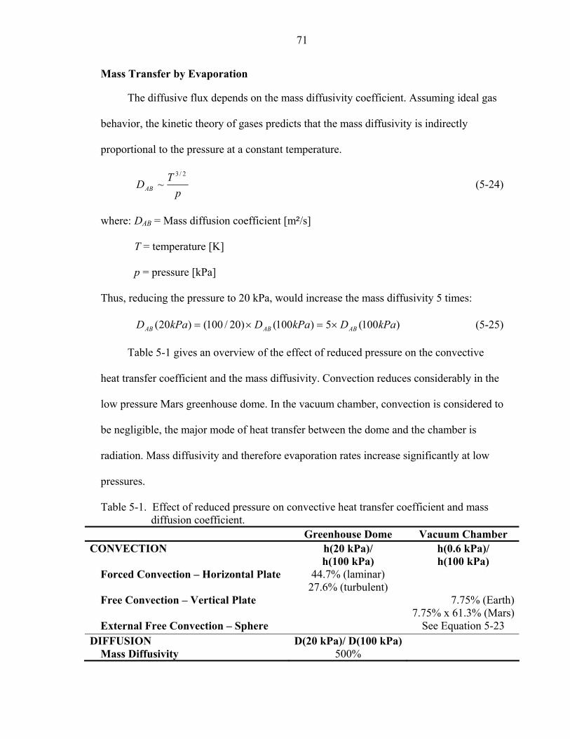
71
Mass Transfer by Evaporation
The diffusive flux depends on the mass diffusivity coefficient. Assuming ideal gas
behavior, the kinetic theory of gases predicts that the mass diffusivity is indirectly
proportional to the pressure at a constant temperature.
pTDAB
2/3
~ (5-24)
where: DAB = Mass diffusion coefficient [m²/s]
T = temperature [K]
p = pressure [kPa]
Thus, reducing the pressure to 20 kPa, would increase the mass diffusivity 5 times:
)100(5)100()20/100()20( kPaDkPaDkPaD ABABAB ×=×= (5-25)
Table 5-1 gives an overview of the effect of reduced pressure on the convective
heat transfer coefficient and the mass diffusivity. Convection reduces considerably in the
low pressure Mars greenhouse dome. In the vacuum chamber, convection is considered to
be negligible, the major mode of heat transfer between the dome and the chamber is
radiation. Mass diffusivity and therefore evaporation rates increase significantly at low
pressures.
Table 5-1. Effect of reduced pressure on convective heat transfer coefficient and mass diffusion coefficient.
Greenhouse Dome Vacuum Chamber CONVECTION h(20 kPa)/
h(100 kPa) h(0.6 kPa)/ h(100 kPa)
Forced Convection – Horizontal Plate 44.7% (laminar) 27.6% (turbulent)
Free Convection – Vertical Plate
7.75% (Earth)7.75% x 61.3% (Mars)
External Free Convection – Sphere See Equation 5-23 DIFFUSION D(20 kPa)/ D(100 kPa)
Mass Diffusivity 500%

72
Development of Low Pressure Psychrometrics for Non-Standard Atmospheres
While most publications address the psychrometric relationships of water vapor
and air for open systems, sea level pressure and Earth’s standard atmosphere composition
(78.08% N2, 20.98% O2, 0.934% Ar, 0.0314% CO2, etc), there is nothing in the theory for
developing the relationships that restricts them to these systems (Shallcross, 1997;
ASHRAE, 2001). In the literature, very few publications are dedicated to altitude effects
on psychrometrics, as barometric pressure decreases with altitude (Haines, 1961;
Hitchcock and Jacoby, 1980; Erickson and Garrett, 1981). Figure 5-1 shows the effect of
reduced pressure on the saturation line of the psychrometric chart. However, psychro-
metric charts that correct for altitude assume that the gas composition is equal to Earth’s.
Compared to the Earth atmosphere, the atmosphere of the greenhouse differs significantly
in terms of pressure and gas constituents. Furthermore, the greenhouse dome is a closed
system, whereas the classic psychrometric relations were developed for open systems.
Figure 5-1. Effect of pressure on the saturation line of an open system with standard
atmosphere composition

73
The psychrometric relations are based on the following fundamental laws of
physics: ideal gas equation of state, conservation of energy, conservation of mass,
Dalton’s law of partial pressures and the Gibbs-Dalton law for energy, enthalpy and
entropy (Gatley, 2002). If the total pressure of the system differs significantly from the
sea level pressure of 101.3 kPa or the dry gas composition differs from the standard Earth
atmosphere, the calculations can be modified to reflect this.
The psychrometric chart is a tool for determining the properties of the moist air and
for visualizing the changes of these properties as a consequence of psychrometric
processes. The-dry bulb temperature is shown on the abscissa of the chart and therefore
the dry-bulb temperature isolines are vertical. The second psychrometric chart coordinate
(the ordinate) is the humidity ratio, which is defined as the ratio of the mass of water
vapor to the mass of the dry air in a moist air sample. Consequently, the humidity ratio
isolines are horizontal. Generally, the properties isolines plotted on a psychrometric chart
are: dry-bulb temperature isolines, humidity ratio isolines, adiabatic saturation
temperature isolines, relative humidity isolines, water vapor saturation curve, enthalpy
isolines and specific volume isolines (Gatley, 2002). The following section develops
general psychrometric relations that can be used for closed low pressure systems and
non-standard gas compositions.
Gas Theory
Equation of state
The classic psychrometric relationships are based on the assumption that moist air
is a mixture of independent perfect gases (i.e. dry air and water vapor), and each gas is
assumed to obey the perfect gas equation of state, where the compressibility factor equals
one. If a low pressure environment is chosen, the perfect gas law applies even better,

74
since the virial coefficients play less role in low pressure gases as the interaction between
molecules is less common. Therefore, the compressibility factor converges to 1 with
decreasing pressure.
...)()()(1 32 +′+′+′+== pDpCpBRTpvZ (5-26)
where: Z = compressibility (Z=1 for perfect gas)
p = pressure
B’,C’,D’ = virial coefficients
Dry gas mixture
The dry gas mixture includes all gas components that remain gaseous and do not
condense in the chosen temperature range. The molecular mass as well as the specific
heat are important parameters for the development of the psychrometric relationships.
If the partial pressures of the dry gas components are known, the content by volume
can be obtained:
dry
idryidry p
p ,, =ψ (5-27)
where: ψdry,i = dry air content of gas component i by volume
pdry,i = partial pressure of gas component i
pdry = total pressure of dry gas
Furthermore, the molecular mass of the dry gas mixture can be calculated:
idryidryidry Mm ,,, ψ= (5-28)
∑= idryidrydry Mm ,,ψ (5-29)
where: mdry,i = mass of gas component i
Mdry,i = molecular mass of gas component i
mdry = total mass of dry gas

75
By calculating the composition of the dry gas mix by mass, the specific heat of the
dry gas mixture is obtained:
totaldry
idryidry m
m
,
,, =ζ (5-30)
idrypidryidryp Cc ,,,,, ζ= (5-31)
∑= idrypidrydryp Cc ,,,, ζ (5-32)
where: ζdry,i = dry air content of gas component i by mass
cp,dry,i = specific heat of gas component i
cp,dry = specific heat of dry gas
The specific enthalpy of dry air is dependent on the temperature of the gas mix:
tch drypdry ,= (5-33)
where: hdry = specific enthalpy of dry air
t = temperature of gas mix
Water vapor component
The molecular mass of water is 18.01528. The specific enthalpy of the saturated
water vapor component is
)805.12501( thg += (5-34)
where: hg = specific enthalpy of water vapor
Construction of Modified Psychrometric Chart
Saturation line
The humidity ratio is defined as the ratio of the mass of water vapor to the mass of
dry air contained in a sample. At saturation, air contains the maximum amount of water:
)()(01528.18
TpTp
mxx
mm
Wdry
ws
drydry
ws
dry
ws == (5-35)

76
where: Ws = humidity ratio at saturation
xws =mole fraction of water vapor in saturated moist air
xdry = mole fraction of dry air in moist air
The total pressure of the moist air is the sum of the partial pressure of the dry air
component and the water vapor.
)()( TpTpp wdrytotal += (5-36)
where: ptotal = total pressure (barometric pressure)
pw = partial pressure of water vapor
The classic psychrometric equations are for open systems where the partial pressure
of the water vapor is small compared to the total pressure. The total pressure is assumed
to be constant even when state change of water occurs, i.e. the partial pressure of dry air
decreases when water vapor pressure increases and vice versa. In the case of a closed
system, the partial pressure of the dry air component depends on the temperature and the
initial conditions, as no dry gas leaves or enters the system boundaries and the volume is
constant:
TTp
Tp drydry 0
0
)( = (5-37)
where: pdry0 = initial pressure of dry air component
T 0 = initial temperature of the gas mixture
Thus, increasing temperature and evaporation lead to an increasing total pressure,
decreasing temperature and condensation to a decreasing total pressure.
The saturated water vapor pressure is a function of the dry-bulb temperature only:
Saturation pressure over ice for the temperature range of –100 to 0° is given by
TCTCTCTCTCCTCpws ln/ln 74
63
52
4321 ++++++= (5-38)

77
where: C1 = -5.6745359E+03
C2 = 6.9325247E+00
C3 = - 9.6778430E-03
C4 = 6.2215701E-07
C5 = 2.0747825E-09
C6 = -9.4840240E-13
C7 = 4.1635019E+00
Saturation pressure over liquid water for the temperature range of 0 to 200° is given by
TCTCTCTCCTCpws ln/ln 133
122
111098 +++++= (5-39)
where: C8 = -5.8002206E+03
C9 = 1.3914993E+00
C10 =- 4.8640239E-02
C11 = 4.1764768E-05
C12 = -1.4452093E-08
C13 = 6.5459673E+00
In both Equations:
ln = natural logarithm
pws= saturation pressure [Pa]
T = absolute temperature [K]
Humidity isolines
The relative humidity is the ratio of the mole fraction of water vapor in a given
moist air sample to the mole fraction in an air sample saturated at the same temperature
and pressure:
ptws
w
ptws
w
pp
xx
,,
==φ (5-40)
where: φ = relative humidity

78
The relative humidity isolines are constructed for a given relative humidity and
varying dry-bulb temperatures:
dry
ws
dry
w
dry
w
dry
w
pTp
mm
xx
mmW )(φ
== (5-41)
The degree of saturation equals to the relative humidity for closed systems:
φµ ===ptws
w
pts pp
WW
,,
(5-42)
where: µ = degree of saturation
Specific enthalpy isolines
The specific enthalpy is the sum of the dry gas specific enthalpy plus the specific
enthalpy of the water vapor:
)805.12501(, tWtcWhhh drypgdry ++=+= (5-43)
The lines of constant enthalpy are constructed for a given enthalpy and varying dry
bulb temperatures:
ttch
W dryp
805.12501)( ,
+−
= (5-44)
Specific volume isolines
The specific volume of a gas mixture is defined as the volume of the mixture per
unit dry gas:
drymV
=ν (5-45)
where: v = specific volume of moist air in terms of unit mass of dry air
V = total volume

79
The gas volume as well as the mass of the dry air of a closed system are constant.
Therefore, the specific volume is also constant:
.0
0
constpm
RTpm
RT
drydrydrydry
===ν (5-46)
Vapor pressure isolines
The humidity ratio is related to the water vapor pressure and the partial pressure of
the dry air as follows:
dry
w
dry
w
pp
mmW = (5-47)
Adiabatic saturation temperature isolines
The wet-bulb temperature is considered to be the temperature measured by a
thermometer with the outside surface kept wet. As moist gas passes the thermometer,
some of the liquid evaporates causing the temperature of the wet-bulb thermometer to
drop. As wet-bulb temperature is dependent on the gas velocity in respect to the
thermometer and the radiative heat transfer, it is not possible to predict the wet-bulb
temperature precisely. Consequently, adiabatic saturation temperature is considered in
this document. Adiabatic saturation temperature tad is defined as the temperature at which
water, by evaporating into moist air at a given dry-bulb temperature and absolute
humidity can bring the air to saturation adiabatically at the same temperature tad
(Shallcross, 1997). However, for the air-water system of this document the curves of
adiabatic saturation temperature and wet-bulb temperature coincide. The adiabatic
saturation temperature is related to the humidity ratio by the following correlation:
ad
addrypwetad
ttttcWt
W186.4805.12501
)()381.22501( ,
−+
−−−= (5-48)
where: tad = adiabatic saturation temperature

80
Dew-point temperature isolines
The dew-point temperature is related to the humidity ratio by the following
equation:
dry
dewws
dry
Ws p
Tpmm
W)(
= (5-49)
where: Tdew = dew-point temperature
Table 5-2 lists the psychrometric parameters of the greenhouse dome atmosphere
with the selected composition for the plant experiments. Figure 5-2 shows the
psychrometric chart for the greenhouse dome atmosphere. It can be utilized to determine
the dew-point temperature at which condensation starts to occur on the greenhouse shell.
One important difference from the classical psychrometric chart is that the dew-point
temperature isolines are not horizontal, as the pressure of the dry air changes with
temperature in a closed system.
Table 5-2. Psychrometric parameters of a low pressure atmosphere (76% N2, 20% O2, 4% CO2) with initial conditions of 20 kPa dry air at 20°C and a constant specific volume of 0.004138m³/kg.
Tdry [°C]
Humidity Φ
pWs [Pa]
pW [Pa]
pt [Pa]
w [kg/kgda]
tdew [ºC]
µ h [kJ/kgda]
tad [ºC]
5 100% 872.49 872.49 19849 0.0281 5.02 1 75.6 5.00 10 100% 1228.00 1228.00 20546 0.0389 10.03 1 108.0 10.00 15 100% 1705.45 1705.45 21364 0.0531 15.03 1 149.2 15.00 20 100% 2338.80 2338.80 22339 0.0715 20.01 1 201.5 20.00 25 100% 3169.22 3169.22 23510 0.0953 25.00 1 267.7 25.00 30 100% 4246.03 4246.03 24928 0.1256 29.98 1 350.9 30.00 5 90% 872.49 785.24 19762 0.0253 3.51 0.9 68.5 3.79
10 90% 1228.00 1105.20 20423 0.0350 8.47 0.9 98.2 8.68 15 90% 1705.45 1534.90 21194 0.0478 13.40 0.9 135.8 13.58 20 90% 2338.80 2104.92 22105 0.0644 18.33 0.9 183.4 18.48 25 90% 3169.22 2852.29 23193 0.0858 23.25 0.9 243.4 23.39 30 90% 4246.03 3821.43 24504 0.1130 28.17 0.9 318.8 28.30 5 80% 872.49 697.99 19675 0.0225 1.83 0.8 61.5 2.48
10 80% 1228.00 982.40 20300 0.0311 6.74 0.8 88.4 7.27 15 80% 1705.45 1364.36 21023 0.0425 11.61 0.8 122.3 12.04 20 80% 2338.80 1871.04 21871 0.0572 16.47 0.8 165.2 16.83 25 80% 3169.22 2535.37 22876 0.0762 21.32 0.8 219.2 21.64 30 80% 4246.03 3396.82 24079 0.1005 26.16 0.8 286.7 26.45
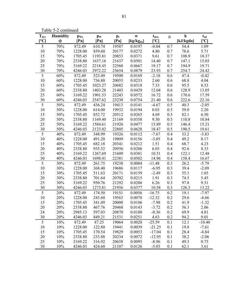
81
Table 5-2 continued Tdry [°C]
Humidity Φ
pWs [Pa]
pW [Pa]
pt [Pa]
w [kg/kgda]
tdew [ºC]
µ h [kJ/kgda]
tad [ºC]
5 70% 872.49 610.74 19587 0.0197 -0.04 0.7 54.4 1.09 10 70% 1228.00 859.60 20177 0.0272 4.80 0.7 78.6 5.71 15 70% 1705.45 1193.81 20853 0.0371 9.61 0.7 108.9 10.37 20 70% 2338.80 1637.16 21637 0.0501 14.40 0.7 147.1 15.03 25 70% 3169.22 2218.45 22560 0.0667 19.17 0.7 194.9 19.71 30 70% 4246.03 2972.22 23654 0.0879 23.93 0.7 254.7 24.42 5 60% 872.49 523.49 19500 0.0169 -2.18 0.6 47.4 -0.42
10 60% 1228.00 736.80 20055 0.0233 2.60 0.6 68.8 4.04 15 60% 1705.45 1023.27 20682 0.0318 7.33 0.6 95.5 8.53 20 60% 2338.80 1403.28 21403 0.0429 12.04 0.6 128.9 13.05 25 60% 3169.22 1901.53 22243 0.0572 16.72 0.6 170.6 17.59 30 60% 4246.03 2547.62 23230 0.0754 21.40 0.6 222.6 22.16 5 50% 872.49 436.24 19413 0.0141 -4.67 0.5 40.3 -2.05
10 50% 1228.00 614.00 19932 0.0194 0.03 0.5 59.0 2.20 15 50% 1705.45 852.72 20512 0.0265 4.69 0.5 82.1 6.50 20 50% 2338.80 1169.40 21169 0.0358 9.30 0.5 110.8 10.84 25 50% 3169.22 1584.61 21926 0.0477 13.89 0.5 146.4 15.21 30 50% 4246.03 2123.02 22805 0.0628 18.47 0.5 190.5 19.61 5 40% 872.49 348.99 19326 0.0112 -7.67 0.4 33.2 -3.83
10 40% 1228.00 491.20 19809 0.0156 -3.05 0.4 49.2 0.17 15 40% 1705.45 682.18 20341 0.0212 1.51 0.4 68.7 4.23 20 40% 2338.80 935.52 20936 0.0286 6.03 0.4 92.6 8.33 25 40% 3169.22 1267.69 21609 0.0381 10.51 0.4 122.1 12.48 30 40% 4246.03 1698.41 22381 0.0502 14.96 0.4 158.4 16.67 5 30% 872.49 261.75 19238 0.0084 -11.48 0.3 26.2 -5.79
10 30% 1228.00 368.40 19686 0.0117 -6.95 0.3 39.4 -2.09 15 30% 1705.45 511.63 20171 0.0159 -2.49 0.3 55.3 1.65 20 30% 2338.80 701.64 20702 0.0215 1.91 0.3 74.5 5.45 25 30% 3169.22 950.76 21292 0.0286 6.26 0.3 97.8 9.31 30 30% 4246.03 1273.81 21956 0.0377 10.58 0.3 126.3 13.22 5 20% 872.49 174.50 19151 0.0056 -16.75 0.2 19.1 -7.97
10 20% 1228.00 245.60 19563 0.0078 -12.32 0.2 29.6 -4.66 15 20% 1705.45 341.09 20000 0.0106 -7.98 0.2 41.9 -1.32 20 20% 2338.80 467.76 20468 0.0143 -3.72 0.2 56.3 2.06 24 20% 2985.13 597.03 20870 0.0180 -0.36 0.2 69.9 4.81 30 20% 4246.03 849.21 21531 0.0251 4.63 0.2 94.2 9.01 5 10% 872.49 87.25 19064 0.0028 -25.59 0.1 12.1 -10.40
10 10% 1228.00 122.80 19441 0.0039 -21.25 0.1 19.8 -7.61 15 10% 1705.45 170.54 19829 0.0053 -17.04 0.1 28.4 -4.84 20 10% 2338.80 233.88 20234 0.0072 -12.95 0.1 38.2 -2.06 25 10% 3169.22 316.92 20658 0.0095 -8.96 0.1 49.3 0.75 30 10% 4246.03 424.60 21107 0.0126 -5.03 0.1 62.1 3.61

82
0.00
0.02
0.04
0.06
0.08
0.10
0.12
0 5 10 15 20 25 30
Dry Bulb Temperature tdry [°C]
Hum
idity
Rat
io w
[kg m
oist
ure/k
g dry
air]
225
200
125
75
50
25
5°C
10°C
tdew = 25°C
tdew = 20°C
tdew = 15°C
tdew = 10°C
tdew = 5°C
tdew = 0°C
15°C
20°C175
150
100
h = 250 kJ/kgdry tad(=twet) = 25°C
0°C
Figure 5-2. Psychrometric chart of low pressure atmosphere (76% N2, 20% O2, 4% CO2) with initial conditions of 20 kPa dry air at
20°C and a constant specific volume of 0.004138m³/kg.

83
One–dimensional Steady State Heat Transfer Model of the Greenhouse Dome
Overall Thermal Resistance Model
A one-dimensional steady state analysis was selected as heat transfer model. The
heat inside of the greenhouse produced by the absorbed growth light radiation and the
heating system is transferred to the outside in the following steps. First convection heat
transfer takes place between the air and the greenhouse inner shell, then heat is
transferred through the greenhouse dome by conduction. Heat transfer between the
greenhouse surface and the inner chamber wall occurs mainly due to radiation. Natural
convection of the outside dome and the interior chamber walls is negligible as the
convection coefficient is reduced significantly by the low pressure of 0.6 kPa (see Table
5-1). The effect of low pressure on convective heat transfer has been discussed
extensively at the beginning of this Chapter. Heat transfer through the vacuum chamber
occurs by conduction. Finally, heat is removed from the vacuum chamber wall by
convection. At the same time, heat is also transferred out of the greenhouse through the
dome base. Thick foam insulation had been installed under the base to minimize the heat
loss through the floor.
The equivalent thermal circuit concept is a useful tool for the development of a
one-dimensional steady state heat transfer model. The thermal resistance is defined as the
ratio of the temperature difference (the driving potential) to the corresponding heat
transfer rate. Figure 5-3 depicts the modes of heat transfer and states the equivalent
thermal resistance circuit.

84
Figure 5-3. Heat transfer of greenhouse dome and thermal resistance circuit.
Individual Thermal Resistances and Thermal Coefficients
The total heat flux out of the greenhouse dome is the sum of the absorbed light plus
the heat added by the heating coil. The heat flux is the ratio of the temperature difference
to the total resistance:
totalLightHeatertotal R
TTQQQ 93 −
=+= (5-50)

85
In analog to the electric circuit the total resistance is determined by the series-
parallel configuration of the individual resistances:
5
98764321
111 R
RRRRRRRR
Rtotal +
++++
+++
= (5-51)
The conduction resistance R7 is very large compared to the other resistances as the
dome base is very well insulated. Thus, the total resistance reduces to:
54321 RRRRRRtotal ++++= (5-52)
where: 211
231 2
1rhQ
TTR
total π=
−= = Convection heat transfer
⎟⎟⎠
⎞⎜⎜⎝
⎛−=
−=
2125
522
112
1rrkQ
TTR
total π= Conduction heat transfer
⎟⎟⎠
⎞⎜⎜⎝
⎛⎟⎟⎠
⎞⎜⎜⎝
⎛ −+
++=
−=
Chamber
stotal
Ar
rTTTTQTT
R
22
6
6
5
22
26
2565
653
211
2))((1
πε
εε
πσ= Radiation heat transfer
Chambertotal AkS
QTT
R67
764 =
−= = Conduction heat transfer
Chambertotal AhQTT
R7
975
1=
−= = Convection heat transfer
r1 = inner dome radius [m]
r2 = outer dome radius [m]
h1 = convection coefficient dome inside [W m-2 K-1]
k25 = conduction coefficient dome [W m-1 K-1]
σs = Stefan-Boltzmann constant [5.670 * 10-8 W m-2 K-4]
εs = emissivity of greenhouse dome outside [-]
ε6 = emissivity of chamber inside [-]
S = thickness of chamber [m]

86
k67 = conduction coefficient chamber [W m-1 K-1]
Achamber = Area of chamber [m²]
h7 = convection coefficient chamber outside [W m-2 K-1]
The thermal resistances and coefficients, defined above, can be solved straight-
forward by inserting the steady state temperatures data of the Galactic lettuce experiment
and the dimensions of the dome and chamber. Table 5-3 lists the temperature data at the
selected locations. Table 5-4 gives an overview of the calculated thermal resistances and
heat transfer coefficients. It can be observed that the data are different for the case when
the light is switched on, compared to the light being switched off. This results from the
temperature differences for both cases. The temperatures of the surfaces are higher when
the light is switched on, because part of the radiation is absorbed by the dome shell and
chamber wall.
The radiation coefficients ε5 and ε6 depend on each other and the equation cannot
be solved without knowing one of them (see Figures 5-4 and 5-5). As the polycarbonate
dome is very transparent a high emissivity of 0.9 was chosen, resulting in an emissivity
value of the chamber of 0.55 for the light turned off and 0.48, when the light is turned on.
Table 5-3. Steady state temperature data of the long-term experiment involving Galactic
lettuce plants. Freezer Temp.
[ºC]
Light Heating Power
[W]
Air T3
[ºC]
Fan T4
[ºC]
Shell Inside
T2 [ºC]
Shell Outside T5 [ºC]
Inside Wall T6
[ºC]
Outside Wall
Middle T7 [ºC]
Outside Wall
Bottom T8 [ºC]
Chamber Air T9
[ºC]
-20 off 119 19.68 24.42 13.81 3.47 -16.73 -18.83 -19.51 -20.01 -20 on 40 20.12 22.16 15.61 8.35 -11.99 -16.04 -19.16 -19.96
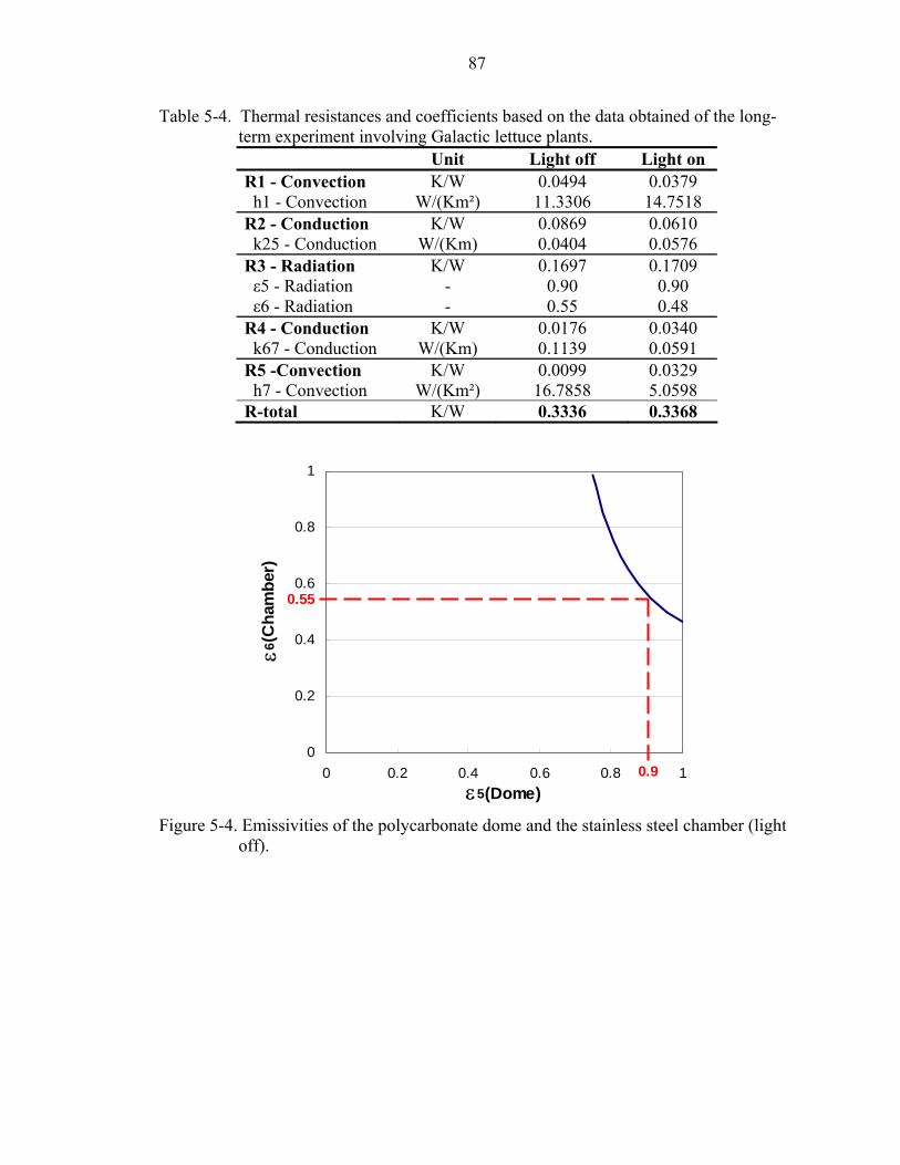
87
Table 5-4. Thermal resistances and coefficients based on the data obtained of the long-term experiment involving Galactic lettuce plants. Unit Light off Light on R1 - Convection K/W 0.0494 0.0379 h1 - Convection W/(Km²) 11.3306 14.7518 R2 - Conduction K/W 0.0869 0.0610 k25 - Conduction W/(Km) 0.0404 0.0576 R3 - Radiation K/W 0.1697 0.1709 ε5 - Radiation - 0.90 0.90 ε6 - Radiation - 0.55 0.48 R4 - Conduction K/W 0.0176 0.0340 k67 - Conduction W/(Km) 0.1139 0.0591 R5 -Convection K/W 0.0099 0.0329 h7 - Convection W/(Km²) 16.7858 5.0598 R-total K/W 0.3336 0.3368
0
0.2
0.4
0.6
0.8
1
0 0.2 0.4 0.6 0.8 1ε5(Dome)
ε6(C
ham
ber)
0.55
0.9
Figure 5-4. Emissivities of the polycarbonate dome and the stainless steel chamber (light
off).

88
0
0.2
0.4
0.6
0.8
1
0 0.2 0.4 0.6 0.8 1ε5(Dome)
ε6(C
ham
ber)
0.48
0.9
Figure 5-5. Emissivities of the polycarbonate dome and the stainless steel chamber (light
on).
The thermal coefficients of Table 5-4 and the dimensions of the dome and the
chamber are entered into a simulation module programmed in LabView. As the radiation
resistance varies with the temperature of the dome and the chamber, a direct
determination of the steady-state temperatures is not possible. A loop recalculates the
temperatures beginning from the initial conditions until steady state is reached. Table 5-5
lists the simulated temperatures at the selected locations.

89
Table 5-5. Simulated temperatures based on the thermal resistance model. Freezer Temp.
[ºC]
Lights (0=off, 1=on)
Heating Power
[W]
Air/ Plant
T3 [ºC]
Shell Inside
T2 [ºC]
Shell Outside T5 [ºC]
Inside Wall T6
[ºC]
Outside Wall T7
[ºC]
Chamber Air T9
[ºC]
0 0 26 8.28 7.00 4.74 0.72 0.26 0.00 0 0 51 16.03 13.51 9.08 1.41 0.51 0.00 0 0 77 23.89 20.09 13.40 2.12 0.76 0.00 0 0 103 31.57 26.48 17.54 2.84 1.02 0.00
-10 0 26 -1.26 -2.54 -4.80 -9.28 -9.74 -10.00 -10 0 51 6.88 4.36 -0.07 -8.59 -9.49 -10.00 -10 0 77 15.10 11.30 4.61 -7.88 -9.24 -10.00 -10 0 103 23.10 18.02 9.07 -7.16 -8.98 -10.00 -20 0 51 -2.15 -4.67 -9.10 -18.59 -19.49 -20.00 -20 0 77 6.48 2.67 -4.02 -17.88 -19.24 -20.00 -20 0 103 14.83 9.75 0.80 -17.16 -18.98 -20.00 -20 0 128 22.64 16.32 5.21 -16.47 -18.73 -20.00 -10 1 0 16.14 13.14 8.33 -4.71 -7.40 -10.00 -10 1 26 24.08 20.10 13.70 -2.97 -6.54 -10.00 -10 1 51 31.47 26.54 18.62 -1.30 -5.72 -10.00 -10 1 77 38.93 33.01 23.51 0.44 -4.86 -10.00 -20 1 0 7.55 4.55 -0.26 -14.71 -17.40 -20.00 -20 1 26 15.82 11.84 -5.44 -12.97 -16.54 -20.00 -20 1 51 23.49 18.56 10.64 -11.30 -15.72 -20.00 -20 1 77 31.21 25.29 15.79 -9.56 -14.86 -20.00 -20 1 103 38.69 31.79 20.69 -7.82 -14.01 -20.00
Table 5-6 compares the temperature values obtained through the simulation to the
temperatures measured during the initial heat transfer experiments. The model works well
for high heating power. Furthermore, the errors are smaller when the light is turned on
compared to the light being turned off. The main contribution to the difference between
the measured and simulated values is the assumption that the heat transfer is only
occurring in one direction. Thus, the vertical temperature distribution of the greenhouse
air and therefore the greenhouse shell is not accounted for.
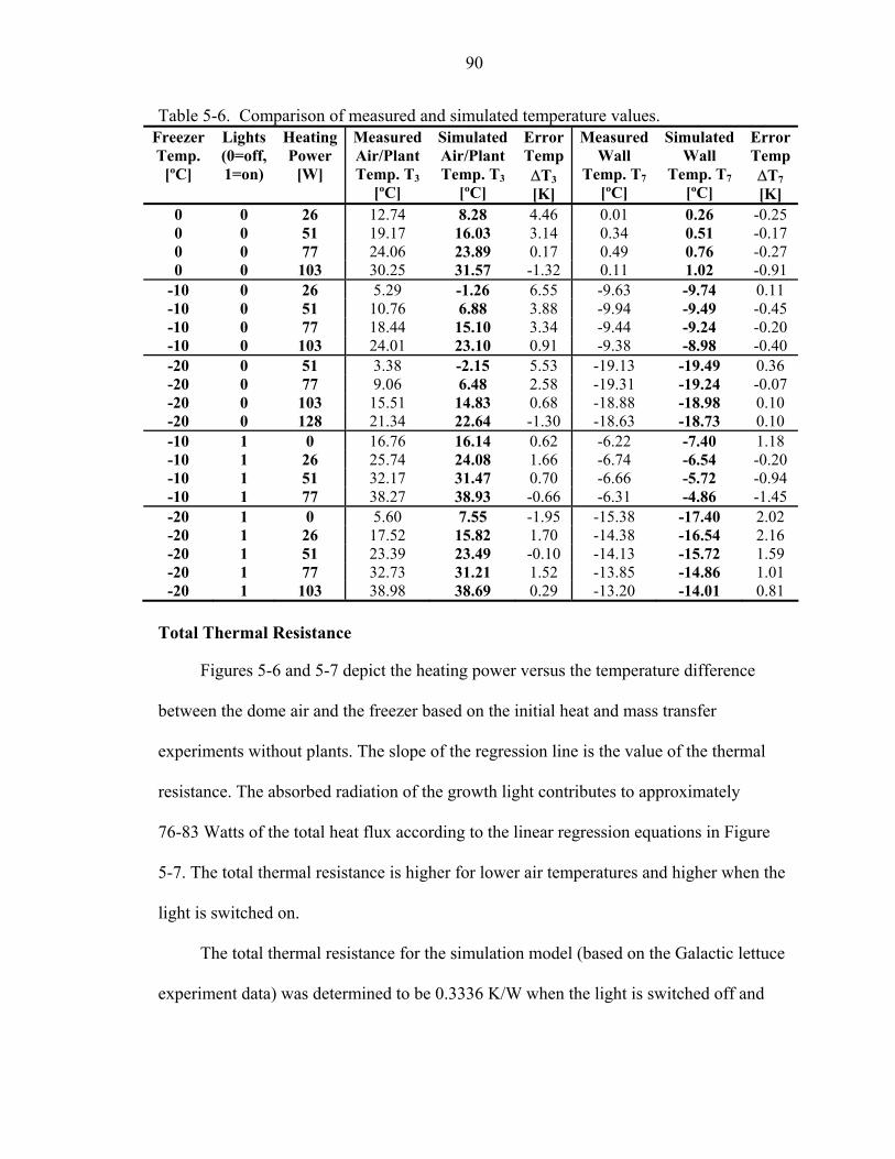
90
Table 5-6. Comparison of measured and simulated temperature values. Freezer Temp.
[ºC]
Lights (0=off, 1=on)
Heating Power
[W]
Measured Air/Plant Temp. T3
[ºC]
Simulated Air/Plant Temp. T3
[ºC]
Error Temp ∆T3 [K]
Measured Wall
Temp. T7 [ºC]
Simulated Wall
Temp. T7 [ºC]
Error Temp ∆T7 [K]
0 0 26 12.74 8.28 4.46 0.01 0.26 -0.25 0 0 51 19.17 16.03 3.14 0.34 0.51 -0.17 0 0 77 24.06 23.89 0.17 0.49 0.76 -0.27 0 0 103 30.25 31.57 -1.32 0.11 1.02 -0.91
-10 0 26 5.29 -1.26 6.55 -9.63 -9.74 0.11 -10 0 51 10.76 6.88 3.88 -9.94 -9.49 -0.45 -10 0 77 18.44 15.10 3.34 -9.44 -9.24 -0.20 -10 0 103 24.01 23.10 0.91 -9.38 -8.98 -0.40 -20 0 51 3.38 -2.15 5.53 -19.13 -19.49 0.36 -20 0 77 9.06 6.48 2.58 -19.31 -19.24 -0.07 -20 0 103 15.51 14.83 0.68 -18.88 -18.98 0.10 -20 0 128 21.34 22.64 -1.30 -18.63 -18.73 0.10 -10 1 0 16.76 16.14 0.62 -6.22 -7.40 1.18 -10 1 26 25.74 24.08 1.66 -6.74 -6.54 -0.20 -10 1 51 32.17 31.47 0.70 -6.66 -5.72 -0.94 -10 1 77 38.27 38.93 -0.66 -6.31 -4.86 -1.45 -20 1 0 5.60 7.55 -1.95 -15.38 -17.40 2.02 -20 1 26 17.52 15.82 1.70 -14.38 -16.54 2.16 -20 1 51 23.39 23.49 -0.10 -14.13 -15.72 1.59 -20 1 77 32.73 31.21 1.52 -13.85 -14.86 1.01 -20 1 103 38.98 38.69 0.29 -13.20 -14.01 0.81
Total Thermal Resistance
Figures 5-6 and 5-7 depict the heating power versus the temperature difference
between the dome air and the freezer based on the initial heat and mass transfer
experiments without plants. The slope of the regression line is the value of the thermal
resistance. The absorbed radiation of the growth light contributes to approximately
76-83 Watts of the total heat flux according to the linear regression equations in Figure
5-7. The total thermal resistance is higher for lower air temperatures and higher when the
light is switched on.
The total thermal resistance for the simulation model (based on the Galactic lettuce
experiment data) was determined to be 0.3336 K/W when the light is switched off and

91
0.3368 K/W when the light is being turned on. Those data points fit well into the total
resistance range determined in Figures 5-6 and 5-7.
∆T = 0.3517*QhR² = 0.9954
∆T = 0.3349*QhR2 = 0.9993
∆T = 0.3194*QhR2 = 0.9996
25
30
35
40
45
50
70 90 110 130 150
Qheating [W]
∆T
(Tai
r-Tf
reez
er) [
K]T Air = 15 ºC
T Air = 20 ºC
T Air = 25 ºC
Figure 5-6. Required heating power versus temperature difference of the dome air to the
freezer. Slope of linear regression is the total thermal resistance (light off).
∆T = 0.3211*(Qh + 83.02024)R2 = 0.9962
∆T = 0.3425*(Qh + 77.45635)R2 = 0.9967
∆T = 0.3640*(Qh + 76.2841)R2 = 0.9971
25
30
35
40
45
50
0 10 20 30 40 50 60
Qheating [W]
∆T
(Tai
r-Tfr
eeze
r) [K
]
T Air = 15 ºC
T Air = 20 ºC
T Air = 25 ºC
Figure 5-7. Required heating power versus temperature difference of the dome air to the
freezer. Slope of linear regression is the total thermal resistance (light on).

92
Comparison of Radiation and Convection in the Chamber at Mars Pressure
One assumption of the thermal resistance model was that inside the vacuum
chamber, at a low pressure of 0.6 kPa, convection is much smaller than radiation and
therefore convection was neglected. By comparing the heat flux through radiation to the
heat flux through convection, it can be verified if the assumption was correct.
In order to calculate the convective heat loss of the dome sphere and the chamber
wall, the flow condition has to be analyzed first, by determining the Rayleigh number
(see Equation 5-22). The Rayleigh number is below the critical Rayleigh number for
convection of the dome as well as for the chamber, therefore the flow is laminar in both
cases. The convection coefficient of the dome is calculated with Equation 5-23 and the
coefficient of the chamber wall with Equation 5-18. The convection heat loss is 3.9 W for
the dome and 12.2 W for the chamber wall. Compared to the radiation heat loss of
119 W, the convection heat loss is only 3.3% for the dome and 10.3% for the chamber
wall. Thus, the assumption that convective heat transfer can be neglected is correct, if the
radiation heat loss is relatively high. If the power of the heating system decreases and the
difference between the chamber wall and dome temperatures is much smaller, convective
heat loss plays a bigger role. This is the major reason, why in Table 5-6 the difference of
the simulated and the measured values increases for low heating power. Table 5-7 lists
the calculated values for the comparison of the convective heat transfer inside of the
vacuum chamber to the radiation heat transfer.

93
Table 5-7. Comparison of convection heat transfer to radiation heat transfer in the chamber at a pressure of 0.6 kPa.
Shell Outside T5
[ºC] Air Chamber T∞
[ºC] Inside Wall T6
[ºC]
Light on 8.35 -5.995 -11.99 Light off 3.47 -8.365 -16.73
Convection Dome Ra Racrit Flow hconv Qconv Qrad Qconv/Qrad
Light on 6.30E+04 1011 laminar 0.2072 3.8577 119 3.25% Light off 6.37E+04 1011 laminar 0.2077 3.8393 119 3.26%
Convection Chamber Wall Ra Racrit Flow hconv Qconv Qrad Qconv/Qrad
Light on 5.06E+04 109 laminar 0.1897 12.1868 119 10.28% Light off 5.15E+04 109 laminar 0.1905 12.1578 119 10.31%
Transient Heat Transfer Model for Greenhouse Temperature Simulation
For the transient heat transfer model, the overall system is split up into the
greenhouse atmosphere, the greenhouse dome, the vacuum chamber and the greenhouse
base plate. Four differential equations (5-53 to 5-56) are set up based on the energy
balance of the four sub-systems. The change of the internal energy is equal to the sum of
the heat fluxes into and out of the system due to energy conservation.
)]()([)( 13125313
13 nn
basenn
domehrad
nn
atmp TTAhTTAhQQt
TTVc −+−−+=
∆−+
ρ (5-53)
where: T3 n+1 = temperature of greenhouse atmosphere at next time step [K]
T3 n = temperature of greenhouse atmosphere at current time step [K]
∆t = time step [s]
cp,atm = specific heat of greenhouse atmosphere [J/kg K]
ρatm = density of greenhouse atmosphere at 20 kPa [kg/m³]
Vatm = volume of greenhouse atmosphere [m³]
Qrad = heat gain from radiation [W]
Qh = heat gain from heating system [W]

94
)()()( 6725253125
125 nn
radradnn
dome
nn
domep TTAhTTAht
TTVc −−−=
∆−+
ρ
(5-54)
where: T25 n+1 = temperature of dome shell at next time step [K]
T25 n = temperature of dome shell at current time step [K]
cp,dome = specific heat of polycarbonate dome shell [J/kg K]
ρdome = density of polycarbonate dome shell [kg/m³]
Vdome = volume of polycarbonate dome shell [m³]
)()()( 677672567
167 n
freeezern
chambernn
radrad
nn
chamberp TTAhTTAht
TTVc −−−=
∆−+
ρ (5-55)
where: T67 n+1 = temperature of vacuum chamber at next time step [K]
T67 n = temperature of vacuum chamber at current time step [K]
cp,chamber = specific heat of stainless steel vacuum chamber [J/kg K]
ρchamber = density of stainless steel vacuum chamber [kg/m³]
Vchamber = volume of stainless steel vacuum chamber [m³]
)()( 1311
11 nn
base
nn
basep TTAht
TTVc −=
∆−+
ρ
(5-56)
where: T1 n+1 = temperature of base at next time step [K]
T1n = temperature of base at current time step [K]
cp,base = specific heat of aluminum dome base [J/kg K]
ρbase = density of aluminum dome base [kg/m³]
Vbase = volume of aluminum dome base [m³]

95
The equations above are based on the assumption that the conduction resistance of
the dome, the vacuum chamber and the base plate are very small and therefore the inside
and outside temperatures are lumped into one equivalent temperature, T25, T67 and T1
respectively. Furthermore, the dome base plate is considered to be perfectly insulated as
it was assumed for the steady state heat transfer model.
The four differential equations contain the four unknown temperature variables
T3n+1
, T25 n+1, T67
n+1and T1 n+1. With the initial conditions of the four temperature
variables, the system can be solved. Figure 5-8, Figure 5-9 and Figure 5-10 compare the
simulation data to the experimental data for three different heating power conditions.
In all three cases the temperature rise of the simulation is much slower than in the
experiment, i.e. it takes longer for the air and dome temperature to reach steady state.
Consequently, the thermal inertia is higher for the simulation compared to the
experimental data. Furthermore, it can be observed that the air temperature experiences a
sudden rise at the beginning of the simulation as the difference between the energy gain
by heating and the energy loss by convection is relatively high. The steady-state
temperatures of the simulation are lower than the steady-state temperatures of the
experiment. The same phenomenon was also seen in the thermal resistance model results.
The transient heat transfer model is a good first approach to simulate the transient
temperature variations of the experiment. In combination with the psychrometric model,
the state of the greenhouse air can be assessed and occurrence of condensation can be
predicted. Figure 5-11 shows the LabView Front Panel for the overall model. A
condensation warning appears if the greenhouse shell temperature is below the dew point
temperature.

96
-15
-10
-5
0
5
10
15
20
0 50 100 150 200Time [min]
Tem
pera
ture
[°C
]
Tair- ExperimentTair - SimulationTdome-ExperimentTdome - SimulationTchamber - ExperimentTchamber - Simulation
Figure 5-8. Simulation of greenhouse atmosphere, dome and vacuum chamber
temperatures (light off, 51W heating power, -10° C freezer temperature).
-15
-10
-5
0
5
10
15
20
0 50 100 150 200 250 300Time [min]
Tem
pera
ture
[°C] Tair - Experiment
Tair - SimulationTdome - ExperimentTdome - SimulationTchamber - ExperimentTchamber - Simulation
Figure 5-9. Simulation of greenhouse atmosphere, dome and vacuum chamber
temperatures (light off, 77 W heating power, -10° C freezer temperature).

97
-15
-10
-5
0
5
10
15
20
25
0 50 100 150 200 250 300 350 400
Time [min]
Tem
pera
ture
[°C] Tair - Experiment
Tair - Simulation
Tdome - Experiment
Tdome - Simulation
Tchamber - Experiment
Tchamber - Simulation
Figure 5-10. Simulation of greenhouse atmosphere, dome and vacuum chamber
temperatures (light off, 103 W heating power, -10° C freezer temperature).
Figure 5-11. LabView front panel of overall model for simulation.

98
CHAPTER 6 RESULTS AND CONCLUSION
An understanding of the heat and mass transfer of a Mars greenhouse is essential to
develop the environmental control system. The environmental control system is
responsible for keeping the atmosphere parameters in a range where plant growth is
productive.
In this research, a Mars chamber was developed simulating the environment on
Mars. A small scale Mars greenhouse was exposed to the simulated Mars environment.
Tests included experiments on the heat and mass transfer without and with plants. The
data obtained through the thermal experiments without plants were used to refine the gas
composition and temperature control algorithm. Furthermore, the temperature distribution
data within the greenhouse and the chamber were utilized in the model development.
Two sets of plant experiments were successfully conducted. The mid-term
experiment involved eight buttercrunch lettuce plants that were exposed to the low
pressure Mars greenhouse environment for 36 hours. Temperature, pressure and
atmosphere composition of the greenhouse and the simulated Mars environment were
controlled. Evapo-transpiration, relative humidity and light levels were measured
continuously. One plant started to wilt as the water supply ceased. The long-term
experiments involved Galactic lettuce plants that were exposed to the low pressure Mars
greenhouse environment for 7 days. After one day of continuous exposure to the growth
light, a day-night cycle of 12 hours was implemented. The temperature of the greenhouse
shell decreased significantly during the night cycle, resulting in the formation of

99
condensation and frost, especially in the lower colder part of the greenhouse. Relative
humidity also decreased during the night cycle as more water condensed than evaporated.
The plants showed no significant visible damage after seven days, only minor wilting was
observed as the water supply was depleted.
Data from the experiments were analyzed to develop a thermal resistance model
that can be used to predict steady-state greenhouse temperatures for various Mars
environment conditions. The analytical data of the model fitted well with the
experimental data for low freezer temperatures, i.e., high temperature differences
between the Mars environment and the greenhouse temperature, as the thermal resistance
model was based on the assumption that at low pressures convection is insignificant
compared to radiation heat transfer. The transient heat transfer model was utilized to
simulate the transient temperature variations of the equipment over time.
Low pressure psychrometric relations were developed for closed systems at various
gas compositions other than the standard atmosphere. The psychrometric model can be
used to predict the state of the moist air. Knowledge of the psychrometric parameters is
especially important for the prediction of the occurrence of condensation.

100
CHAPTER 7 FUTURE WORK
The results of this study show that there is a vertical temperature and humidity
stratification of the greenhouse dome atmosphere. The installation of a heater on the cold
greenhouse aluminum base and improved insulation would lead to a more uniform
atmosphere, preventing the build-up of condensate and ice in the lower part of the
greenhouse (see Figure 7-1).
If a passive humidity control system is selected, the water should condense on the
greenhouse shell above the gravity-driven recollection funnel. At the same time,
condensate should not collect above the plant level as it would interfere with the radiation
required for plant growth. Another option of condensing the water out of the atmosphere
would be to pipe air out of the greenhouse to a heat exchanger with the Mars environment
and to feed back the water and the dried air separately into the dome. Temperature of the
condensation surface should be monitored carefully as the temperature should be below
the dew point but above the freezing point. Gravity driven water collection systems
should be applied where possible as they work in the low-gravity Mars environment and
avoid the installation of pumps.
The duration of the experiments was limited by the decreasing water supply to the
plants. An efficient water recycling system, that collects the condensate and feeds it back
to the plants would minimize the required resupply of water from the outside and increase
the length of the experiment.

101
Future research should also include full growth cycles of the plants from seeds to
maturity as small plants are much more vulnerable to environmental changes. A
simulated day-night cycle with gradual intensity increase of the growth light could be
implemented, as it would replicate the Mars environment more accurately.
A)
B) Figure 7-1. Ice building up on the bottom part of the greenhouse shell. A) Overview. B)
Detailed view of the ice-crystals.

102
APPENDIX A STRUCTURAL ANALYSIS OF DOME SHELL, BASE PLATE AND CYLINDRICAL
CALIBRATION CHAMBER
Structural Analysis of the Spherical Greenhouse Dome
Most Mars greenhouse experiments utilize enclosures that are under compression,
because they incorporate standard atmosphere on the outside and low pressure inside of
the vessel. In this case, a structural analysis should be performed to avoid a stability
failure under compression. Whereas, the greenhouse dome (operated at 20-25 kPa
pressure) in this project is placed in a vacuum chamber operated at the low Mars pressure
of 0.6 kPa. Therefore, the structural analysis should be performed for a semi-sphere under
tension:
The yield stress of the hemisphere is defined as:
trPcrit=maxσ (A-1)
where: Pcrit = critical pressure [3.67 psi = 0.25 atm.]
r = radius of sphere [21 in (0.53 m)]
t = wall thickness [0.25 in (0.635 cm)]
The yield stress of the sphere of 308.28 psi (2126 kPa) is well below the maximum
yield stress of 1000 psi (6895 kPa). Therefore, the safety factor is 3.24.
Assuming a safety factor of 1.5 leads to the conclusion, that the greenhouse dome
should not be operated at a pressure difference of more than 7.9 psi or 0.5 atm.

103
Structural Analysis of Base Plate for Greenhouse Dome
A ¼ inch aluminum plate serves as the base of the greenhouse dome. It is re-
enforced with aluminum tubes welded to the bottom of the plate. Figure A-1 shows the
bottom view of the dome base plate.
Figure A-1. Bottom view of greenhouse dome base.
For the structural analysis the dome base is split up into four uniformly circular
sectors with 90 degree angles (see Figure A-2). First the structural analysis is performed
of a plate with the main two bracings considered as beams. A second analysis also takes
the additional square bracing into account. The structural analyses of this section are
based upon the equations found in American Aluminum Association (1981).

104
Structural Analysis of the Base Plate without Additional Bracings
The first analysis assumes a triangular load over the full beam depicted in Figure
A-2.
Figure A-2. Triangular load over full beam.
The total load on the sector, i.e., beam, is the area of the triangle and can be
calculated by multiplying the pressure difference by the wedge area:
42
2max πqLLw
W == (A-2)
where: W = total load [lb]

105
wmax = maximum distributed loading [lb/in]
L = length of beam [m]
q = pressure differential [psi]
Therefore, the maximum loading of the beam is:
2maxπqLw = (A-3)
The reactions R1 and R2 at the supports are:
61wLR = (A-4)
32wLR = (A-5)
The bending moment varies with the location x on the beam:
LxLxw
xLL
WxxM6
)()(
3)(
22max22
2
−=−= Lx ≤≤0 (A-6)
The maximum bending moment is encountered at 0.55774 L:
41283.01283.0)5774.0(
3
maxπqLWLLxM === (A-7)
The deflection varies with the location x on the beam:
)7103(180
)( 42222 LxLx
EILWxxdef +−= Lx ≤≤0 (A-8)
The maximum deflection is encountered at 0.5193 L:
EIqL
EIWLLxdef
401304.001304.0)5193.0(
53
maxπ
=== (A-9)

106
Structural Analysis of the Base Plate with Additional Bracings
The second structural analysis also considers the additional bracing in the form of a
square. Similar to the first analysis the plate is split up into four sectors and the main
bracing is considered as a beam (see Figure A-3).
Figure A-3. Trapezoidal load over part of the beam.

107
The load inside of the additional bracing (for x < a) is taken by the interior
bracings, therefore only the distributed load outside the additional bracing (for x>a) is
considered. This leads to a trapezoidal load distribution as shown in Figure A-3.
In this case also Equation A-2 applies, leading to a maximum load of the beam,
similarly to the triangular load distribution (see Equation A-3):
2maxπqL
w = (A-10)
The trapezoidal load on the beam can be calculated by super positioning a uniform
load (see Figure A-4) and a triangular load (see Figure A-5) for x>a.
Figure A-4. First part of superposition: uniform load for x>a.
The uniform load w* is related to the maximum trapezoidal load wmax (defined in
Equation A-10) as follows:
max* wLaw = (A-11)
The reactions R1 and R2 at the supports are:
LwaLR
2*)( 2
1−
= (A-12)
LwaLR
2*)( 22
2−
= (A-13)

108
The bending moment M1 for x<a is:
xRxM 11 )( = ax ≤≤0 (A-14)
xL
aqaLxwL
aaLxM4)(
2)()(
2
max2
2
1π−
=−
= ax ≤≤0 (A-15)
The bending moment M2 for x>a is:
*2
)()()(2
22 wxLLxRxM −−−= Lxa ≤≤ (A-16)
max
222
2 ]2
)(2
))(([)( wLaxL
LxLaLxM −
−−−
= Lxa ≤≤ (A-17)
4])())(([)( 2
22
2πaqxL
LxLaLxM −−
−−= Lxa ≤≤ (A-18)
The second part of the superposition is a triangular load on the beam for x>a as
shown in Figure A-5.
Figure A-5. Second part of superposition: triangular load for x>a.
The maximum triangular load w** is related to the maximum load of the trapezoid
wmax (defined in Equation A-10) as follows:
max1** wLaw ⎟
⎠⎞
⎜⎝⎛ −= (A-19)

109
The reactions R1 and R2 at the supports are:
LwaLR
6**)( 2
1−
= (A-20)
)2(6
**)(6
**)(2
**)( 2
2 aLL
waLL
waLwaLR +−
=−
−−
= (A-21)
The bending moment M1 for x<a is:
xRxM 11 )( = ax ≤≤0 (A-22)
xwLa
LaLx
LwaLxM max
22
1 16
)(6
**)()( ⎟⎠⎞
⎜⎝⎛ −
−=
−= ax ≤≤0 (A-23)
xLaqaLxM ⎟
⎠⎞
⎜⎝⎛ −
−= 1
12)()(
2
1π ax ≤≤0 (A-24)
The bending moment M2 for x>a is:
⎥⎥⎥⎥
⎦
⎤
⎢⎢⎢⎢
⎣
⎡
−−
+
−−
+−−+
−−
−−=*)*)(**(3
**)(**2)()2*(*
)(2)()()( 22
waLaxw
waLaxw
xLaxLwaLxLxLRxM
Lxa ≤≤ (A-25)
⎭⎬⎫
⎩⎨⎧
⎥⎦⎤
⎢⎣⎡ −+
−−−
−−+−
=3
32)()(2
)())(2(6
)(**)(2axLxL
aLxLxLaL
LaLwxM
Lxa ≤≤ (A-26)
⎭⎬⎫
⎩⎨⎧ −+
−−
−+−−
=3
32)(2
)(6
)2)()((**)(2
2axL
aLxL
LaLxLaLwxM Lxa ≤≤ (A-27)
⎭⎬⎫
⎩⎨⎧
−+−−+−−
= )32()()2)(()(12
)( 22
2 axLxLL
aLxLaLqxM π Lxa ≤≤ (A-28)

110
The bending moments M1 and M2 of the trapezoidal load are calculated by
superposition, i.e. summing up the bending moments of the uniform and of the triangular
load:
xLaqaLx
LaqaLxM ⎟
⎠⎞
⎜⎝⎛ −
−+
−= 1
12)(
4)()(
22
1ππ ax ≤≤0 (A-29)
xL
qaLaLxM12
)2()()(2
1π+−
= ax ≤≤0 (A-30)
⎭⎬⎫
⎩⎨⎧
⎥⎦
⎤⎢⎣
⎡−+−−
+−+−−
−−= )32)(()2()(3)]()([
12)()(
222
2 axLxLL
aLaLaxLL
aLqxLxM π
Lxa ≤≤ (A-31)
Figure A-6 shows the bending moments of the beam under a load in form of a
trapezoid. The bending moments are decreasing for increasing distance a of the bracing
from the center of the plate.
Figure A-6. Bending moments of beam for trapezoidal load varies with the distance a of
the additional bracing.

111
The section modulus Sbeam of a 3 x 2 x 1/8 aluminum bar is 0.978 in3 (16.03 cm3)
and the moment of inertia Ix about the x-axis is 1.467 in4 (61.06 cm4) (American
Aluminum Association, 1981). The total moment of inertia of the beam and the plate is
calculated as follows:
22beambeambeamplatePlateplatetotal dAIdAII +++= (A-32)
where: Itotal = total inertia [3.23 in4 (134.44 cm4)]
Iplate = inertia of plate section [ 43
00781.012
25.06 in=× (0.3251 cm4)]
Aplate = area of plate section [1.5 in2 (9.68 cm2)]
dplate=distance to plate centroid[ inAA
AA
platetube
platetube 91.025.1125.35.1
=−+
×+×(2.3cm)]
Ibeam = inertia of beam [1.467 in4 (61.06 cm4)]
Abeam = area of plate section [1.1875 in2 (7.66 cm2)]
dbeam = distance to beam centroid [0.47 in (1.19 cm)]
With the moment of inertia, the section modulus Stotal of the plate and the beam is
defined as:
c
IS total
total = (A-33)
where: Stotal = section modulus of plate and beam[1.34 in3]
c = distance centroid to base [ inAA
AA
platetube
platetube 41.2125.35.1
=+
×+× (6.12 cm)]
The stress is defined as ratio of the bending moment M to the section modulus S:
SM
=σ (A-34)

112
The maximum stress for tension and compression is 16000 psi (110316 kPa).
Applying a safety factor of 1.65, results in a maximum stress of 9700 psi (33879 kPa).
The maximum stress allowed near a welding is 6500 psi (44816 kPa) (American
Aluminum Association, 1981). Table A-1 lists the properties of the stress analysis for the
base plate without and with the additional bracings (at a = 7 in (17.8 cm). Calculations
are done for the beam and for the combination of the beam and the plate. The calculated
stress for the plate without the additional bracings is higher then for the plate with the
bracings. In all cases the stress was below 4000 psi (27579 kPa), i.e. below the maximum
allowed stress of 6500 psi (44816 kPa) near weldings.
Table A-1. Structural analysis of base plate without and with additional bracings. Base plate without bracings ( load in form of triangle over full beam)
L q E Mmax I S def σ [in] [psi] [psi] [in-lb] [in4] [in3] [in] [psi] 21 4 1.05E+07 3732.8 1.47 0.978 1.08E-02 3816.77 21 4 1.05E+07 3732.8 3.23 1.34 4.94E-03 2783.39
Base plate with bracings (load in form of a trapezoid over part of the beam)L a q E Mmax I S def σ
[in] [in] [psi] [psi] [in-lb] [in4] [in3] [in] [psi] 21 7 4 1.05E+07 3429 1.47 0.978 - 3506.13 21 7 4 1.05E+07 3429 3.23 1.34 - 2556.86
Structural Analysis of Cylinder used as Sensor Calibration Chamber
The stability behavior of cylindrical shells loaded by external pressure varies with
length, shell thickness and wall curvature. Their behavior ranges from that of a pure long
cylinder to behavior approaching that of flat plates for short cylinders (Galambos, 1998).
Maximum Allowable Pressure
Calculation of the maximum allowable pressure is the first step to determine
structural failure of a cylinder including axial buckling and wall material yielding. In

113
order to evaluate the maximum allowable pressure, the cylinder has to be classified into
one of the three following categories: short, intermediate or long cylinder.
Short cylinder behavior
The criterion for a cylinder to be classified as a short cylinder is:
⎟⎠⎞
⎜⎝⎛<⎟
⎠⎞
⎜⎝⎛<⎟
⎠⎞
⎜⎝⎛
tD
DL
tD 5.51.1 (A-35)
where: L = length of cylinder [12 in (30.5 cm)]
D = diameter of cylinder [8 in (20.32 cm)]
t = wall thickness [0.25 in (0.635 cm)]
As the length to diameter ratio is 1.5, the cylinder cannot be classified as a short
cylinder, defined by a length to radius ratio between 0.2 and 1.0.
Intermediate cylinder behavior
The criterion for a cylinder to be classified as an intermediate cylinder is:
⎟⎠⎞
⎜⎝⎛<⎟
⎠⎞
⎜⎝⎛<⎟
⎠⎞
⎜⎝⎛
tD
DL
tD 55.05.5 (A-36)
As the length to diameter ratio is 1.5, the cylinder can be classified as an
intermediate cylinder, defined by a length to radius ratio between 1.0 and 3.1.
At the same time, the parameter θ should be between 10 and 32 (=D/t) for an
intermediate cylinder. θ is calculated at 15.4 by utilizing the following equation:
⎟⎠⎞
⎜⎝⎛
⎟⎠⎞
⎜⎝⎛=
tD
DL818.1θ (A-37)
The critical external pressure of an intermediate cylinder is defined as:
⎥⎥⎦
⎤
⎢⎢⎣
⎡⎟⎠⎞
⎜⎝⎛
⎟⎠⎞
⎜⎝⎛
=5.2
6.2
tD
DL
EPcrit (A-38)

114
Therefore, the critical pressure equals 134.7 psi (equivalent to 9.2 atmospheres).
Utilizing a safety factor of 1.5 leads to the conclusion, that the external pressure should
not exceed 89.9 psi (equivalent to 6.4 atmospheres).
Long cylinder behavior
The criterion for a cylinder to be classified as a long cylinder is:
⎟⎠⎞
⎜⎝⎛>⎟
⎠⎞
⎜⎝⎛
tD
DL 1.2 (A-39)
As the length to diameter ratio is 1.5, the cylinder cannot be classified as a long
cylinder, defined by a length to radius ratio above 11.9.
Axial Buckling
After the cylinder has been classified as an intermediate cylinder and the critical
external pressure was determined to be 134.4 psi (927 kPa), the cylinder should be
checked for axial buckling. A safety factor of at least 10 should be applied.
The wall stress should be calculated at the critical pressure:
tDPcrit
axial 4=σ (A-40)
The critical wall stress is defined as:
DEt
crit 21.1. =σ (A-41)
where: E = modulus of elasticity of wall material [450000 psi (3102641 kPa)]
The ratio of the critical wall stress (17015.6 psi (117318 kPa)) to the actual wall
stress (1077.2 psi (7427 kPa) at critical pressure) equals 15.8 fulfilling our design
criterion of a safety factor of 10.

115
Wall Yielding
The cylinder should be checked for wall yielding at the critical external pressure
calculated at 124.4 psi (858 kPa). A safety factor of at least 1.6 is required
For an intermediate cylinder the circumferential stress is defined by:
tDPcrit
ntialcircumfere 4. =σ (A-42)
The ratio of the critical circumferential stress (2154.5 psi (14855 kPa)) to the actual
wall stress (1077.2 psi (7427 kPa) at critical pressure) is determined to be 2.0 fulfilling
our design criterion of a safety factor of 2 for wall yielding.
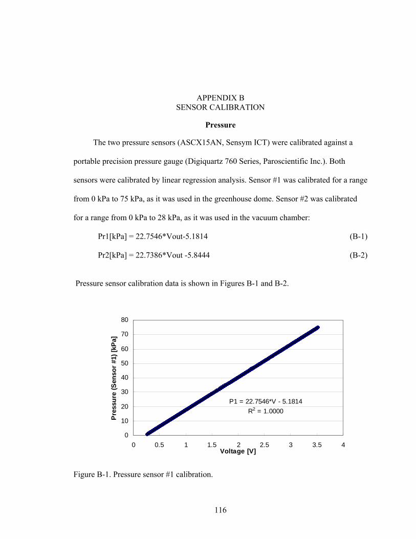
116
APPENDIX B SENSOR CALIBRATION
Pressure
The two pressure sensors (ASCX15AN, Sensym ICT) were calibrated against a
portable precision pressure gauge (Digiquartz 760 Series, Paroscientific Inc.). Both
sensors were calibrated by linear regression analysis. Sensor #1 was calibrated for a range
from 0 kPa to 75 kPa, as it was used in the greenhouse dome. Sensor #2 was calibrated
for a range from 0 kPa to 28 kPa, as it was used in the vacuum chamber:
Pr1[kPa] = 22.7546*Vout-5.1814 (B-1)
Pr2[kPa] = 22.7386*Vout -5.8444 (B-2)
Pressure sensor calibration data is shown in Figures B-1 and B-2.
P1 = 22.7546*V - 5.1814R2 = 1.0000
0
10
20
30
40
50
60
70
80
0 0.5 1 1.5 2 2.5 3 3.5 4Voltage [V]
Pres
sure
(Sen
sor #
1) [k
Pa]
Figure B-1. Pressure sensor #1 calibration.

117
y = 22.7386x - 5.8444R2 = 1.0000
0
5
10
15
20
25
30
0 0.2 0.4 0.6 0.8 1 1.2 1.4 1.6
Sensor Output [V]
Pre
ssur
e (S
enso
r #2)
[kPa
]
Figure B-2. Pressure sensor #2 calibration.
Temperature
The digital temperature sensors (DS18B20, Dallas Semiconductor) were exposed to
a variety of pressure and gas composition combinations. The sensor readings were not
affected by pressure or gas mixture.
Relative Humidity
Relative humidity (RH) measurement is affected by pressure and gas composition
changes. However, the capacitance RH sensors output differed by less than 3% when
compared to the hygrometer standard (HMP 237, Vaisala) as described in Chapter 4 of
this dissertation. Therefore, the factory calibration was used for the four RH sensors:
RH1[%]=(Vout-0.894)/0.0315 (B-3)
RH2[%]=(Vout-0.875)/0.0313 (B-4)
RH3[%]=(Vout-0.894)/0.0315 (B-5)
RH4[%]=(Vout-0.855)/0.0319 (B-6)

118
Carbon Dioxide Concentration
The carbon dioxide sensor (GMP 221, Vaisala) was calibrated under different gas
composition and pressures with the method described in Mu (2005):
CO2 [%] = Slope(P)*Vout + Intercept(P) (B-7)
where: Slope(P) = 0.0267*P2 - 1.9901*P + 41.991
Intercept(P) = -0.0031*P2 + 0.2598*P - 7.179
In contrast to Mu (2005), a parabolic regression fit was chosen for the slope and intercept
equations, because the error was significantly less compared to a linear regression.
Figures B-3 and B-4 depict the calibration of the carbon dioxide sensor.
CO2%(50kPa) = 3.4609*V(50kPa) - 1.3977R2 = 0.9941
CO2%(40kPa) = 4.8602*V(40kPa) - 1.7557R2 = 0.9917
CO2%(30kPa)= 7.2743*V(30kPa) - 2.3438R2 = 0.9881
CO2%(20kPa) = 11.962*V(20kPa) - 3.0986R2 = 0.9891
CO2%(10kPa) = 25.071*V(10kPa) - 4.9404R2 = 0.96450
0.5
1
1.5
2
2.5
3
3.5
0 0.5 1 1.5Sensor Output [V]
Car
bon
Dio
xide
Con
cent
ratio
n [%
]
50 kPa40 kPa30kPa20kPa10kPa
Figure B-3. Carbon dioxide sensor calibration.

119
Intercept = -0.0031*P2 + 0.2598*P - 7.179R2 = 0.9926
Slope = 0.0267*P2 - 1.9901*P + 41.991R2 = 0.9922
-10
-5
0
5
10
15
20
25
30
0 10 20 30 40 50
Pressure [kPa]
Slo
pe/In
terc
ept
Slope
Intercept
Figure B-4. Carbon dioxide sensor calibration.
Oxygen Concentration
The two oxygen sensors (Max250, Maxtec) ware calibrated under different gas
composition and pressures with the same method as the carbon dioxide sensor
(Mu, 2005):
O2 [%]= Slope(P)*mVout + Intercept(P) (B-8)
where: Slope1(P) = 0.023*P2 - 1.6411*P+ 33.25
Intercept1(P) = -0.0069*P2 + 0.5047*P - 8.1629
Slope2(P) = 0.0479*P2 - 3.4467*P + 70.061
Intercept2(P) = -0.0315*P2 + 2.300*P - 45.376
A parabolic regression fit was chosen for the slope and intercept equations, because the
error was significantly less compared to a linear regression. Figures B-5 and B-6 depict
the calibration of the oxygen sensor #1; Figures B-7 and B-8 depict the calibration of the
oxygen sensor #2.

120
O2%(50kPa) = 3.2682*mV(50kPa)+ 1.3388R2 = 0.9988
O2%(40kPa)= 4.1253*mV(50kPa) + 1.0695R2 = 0.9987
O2%(30kPa)= 5.5565*mV(30kPa) + 0.6438R2 = 0.9988
O2%(20kPa) = 8.7876*mV(20kPa) - 0.6745R2 = 0.9994
O2%(10kPa) = 19.419*mV(10kPa) - 3.8516R2 = 0.9988
0
5
10
15
20
25
30
35
0 2 4 6 8 10
Sensor Output [mV]
Oxy
gen
Conc
entra
tion
(Sen
sor
#1) [
%]
50 kPa40 kPa30kPa20kPa10kPa
Figure B-5. Oxygen sensor #1 calibration.
Slope1 = 0.023*P2 - 1.6411*P+ 33.25R2 = 0.9891
Intercept1 = -0.0069*P2 + 0.5047*P - 8.1629R2 = 0.9969
-10
-5
0
5
10
15
20
25
0 10 20 30 40 50
Pressure [kPa]
Slo
pe1/
Inte
rcep
t1
Slope
Intercept
Figure B-6. Oxygen sensor #1 calibration.

121
O2%(50kPa) = 6.4224*mV(50kPa) - 2.151R2 = 0.9985
O2%(40kPa) = 8.3241*mV(40kPa) - 3.5136R2 = 0.9986
O2%(30kPa) = 11.479*mV(30kPa) - 5.7532R2 = 0.999
O2%(20kPa) = 18.619*mV(20kPa) - 11.001R2 = 0.9998
O2%(10kPa)= 40.947*mV(10kPa) - 25.859R2 = 0.99890
5
10
15
20
25
30
35
0 1 2 3 4 5 6
Sensor Output [mV]
Oxy
gen
Conc
entra
tion
(Sen
sor #
2) [%
]
50 kPa40 kPa30kPa20kPa10kPa
Figure B-7. Oxygen sensor #2 calibration.
Slope2 = 0.0479*P2 - 3.4467*P + 70.061R2 = 0.9903
Intercept2 = -0.0315*P2 + 2.300*P - 45.376R2 = 0.9928
-30
-20
-10
0
10
20
30
40
50
0 10 20 30 40 50
Pressure [kPa]
Slop
e2/In
terc
ept2
Slope
Intercept
Figure B-8. Oxygen sensor #2 calibration.
Load Cells
The load cells of the scales were calibrated against standard weights by linear
regression analysis:

122
massScale1 [g] = 188.84 * mVout1 – 682.7 (B-9)
massScale2 [g] = 207.64 * mVout2 - 1259 (B-10)
massScale3 [g] = 189.9 * mVout3 – 624.67 (B-11)
massScale4 [g] = 119.11 * mVout4 – 1222.6 (B-12)
massScale5 [g] = 215.86 * mVout5 – 670.27 (B-13)
The load cell calibration is shown in Figure B-9.
m1 = 188.84*V1 - 682.7R2 = 0.9999
m2 = 207.64*V2 - 1259R2 = 0.9994
m3 = 189.9*V3 - 624.67R2 = 1
m4 = 191.11*V4 - 1222.6R2 = 1
m5 = 215.86*V5 - 670.27R2 = 0.9996
0100200300400500600700800900
1000
2 4 6 8 10
Sensor Output [mV]
mas
s [g
]
Scale 1Scale 2Scale 3Scale 4Scale 5
Figure B-9. Load cell calibration.
Radiation
The light sensor (LI-190SA, LI-Cor Inc.) was exposed to a variety of pressure and
gas composition combinations. The sensor readings were not affected by pressure or gas
mixture. Therefore, the factory calibration was used:
Rad[µmol/(m²s)]=mVout*1000/4.83 (B-14)

123
Amplification of Low Voltage Sensors
The sensors with an output in the milivolt range, such as the oxygen sensor, the
light sensor and the scales had to be amplified in order be read correctly. Signal
amplification was achieved by utilizing Burr-Brown’s Low Power Instrumentation
Amplifier. The amplification was set to 106.38 (50kΩ/470 Ω). The amplification circuit
is shown in Figure B-10.
Figure B-10. Amplifier circuit.

124
LIST OF REFERENCES
Albright, L. D.; Gates, R.D.; Arvanitis, K.G. and Drysdale, A. E. 2001. Plants on Earth and in Space. IEEE Control Systems Magazine 21(5): 28-41.
American Aluminum Association. 1981. Engineering data for aluminum structures. Construction Manual Series. Section 3. Washington, DC.
Andre, M. and Massimino, D. 1992. Growth of plants at reduced pressures. Experiments in wheat: technological advantages and constraints. Advances in Space Research 12(5): 97-106.
Andre, M. and Richaud, C. 1986. Can plants grow in quasi-vacuum? In: CELSS 1985 Workshop. Ames Research Center. NASA Publication TM 88215: 395-404.
American Society of Heating, Refrigeration and Air-Conditioning Engineers (ASHRAE). 2001. Handbook: Fundamentals. SI Edition. Atlanta, GA: ASHRAE.
Boardman, N.K. 1977. Comparative photosynthesis of sun and shade plants. Annual Reviews of Plant Physiology 28: 355-377.
Brown, D. and Lacey, R.E. 2002. A distributed control system for low pressure plant growth chambers. 2002 ASAE Annual International Meeting. Paper No 02-3078. American Society of Agricultural Engineers. Chicago, IL.
Bucklin, R.A.; Fowler, P.A.; Rygalov, V.Y.; Wheeler, R.M.; Mu, Y.; Hublitz, I. and Wilkerson, E.G. 2004. Greenhouse design for the Mars environment: Development of a prototype, deployable dome. Acta Horticulturae 659: 127-134.
Carr, M. H. 1981. The surface of Mars. Yale University Press. New Haven, CT.
Clawson, J. M.; Hoehn, A.; Stodiek, L. S. and Todd, P. 1999. AG-Pod - The integration of existing technologies for efficient, affordable space flight agriculture. 29th International Conference of Environmental Systems. SAE Technical Paper Series, 1999-01-2176. Denver, CO.
Corey, K. A.; Barta, D. J.; Edeen, M.A. and Henninger, D. L. 1997a. Atmospheric leakage and method for measurement of gas exchange rates of a crop stand at reduced pressure. Advances in Space Research 20(10): 1861-1867.

125
Corey, K. A.; Barta, D. J. and Henninger, D. L. 1997b. Photosynthesis and respiration of a wheat stand at reduced atmospheric pressure and reduced oxygen. Advances in Space Research 20(10): 1869-1877.
Corey, K. A.; Barta, J.D. and Wheeler, R. M. 2002. Toward Martian agriculture: Responses of plants to hypobaria. Life Support & Biosphere Science 8: 103-114.
Corey, K. A.; Bates, M.E. and Adams. S.L. 1996. Carbon dioxide exchange of lettuce plants under hypobaric conditions. Advances in Space Research 18 (4/5): 265-272.
Daunicht, H. J. and Brinkjans, H. J. 1996. Plant responses to reduced air pressure: Advanced techniques and results. Advances in Space Research 18 (4/5): 273-281.
Downs, R.J. and Hellmers, H.1975. Environment and the experimental control of plant growth. Academic Press Inc. Ltd. London, UK.
Duffield, B. E. 2003. Advanced life support requirements document. JSC-38571, Revision C, National Aeronautics and Space Administration, Lyndon B. Johnson Space Center. Houston, TX.
Eckart, P. 1996. Spaceflight life support and biospherics. Space Technology Library, Microcosm Press. Torrance, CA.
Erickson, L.R. and Garrett, R.E. 1981. Atmospheric pressure effect on vapor pressure deficit and potential moisture loss for horticultural commodities. Transactions of the ASAE 24: 252-254.
Ferl, R.J.; Schuerger, A.C.; Paul, A.-L.; Gurley, W.B.; Corey, K and Bucklin, R.A. 2002. Plant adaptation to low atmospheric pressures: potential molecular responses. Life Support and Biosphere Science 8: 93-101.
Fowler, P.A.; Bucklin, R.A.; Wheeler, R.M. and Rygalov, V.Y. 2002. Monitoring and control for artificial climate design. International Conference on Environmental Systems. Paper 02ICES-2286. Society of Automotive Engineers. San Antonio, TX.
Galambos, T.V. 1998. Guide to stability criteria for metal structures. 5th Edition. John Wiley and Sons. New York, NY.
Gatley, D. P. 2002. Understanding psychrometrics. American Society of Heating, Refrigeration and Air-Conditioning Engineers (ASHRAE). Atlanta, GA.
Gertner, B. 1999. Mars greenhouse study: Natural vs. artificial lighting. Lockheed Martin Space Mission Systems & Services Science, Engineering, Analysis, and Test. HDID-2G42-1167. Houston, TX.
Goto, E.; Arai, Y. and Omasa, K. 2002. Growth and development of higher plants under hypobaric conditions. International Conference on Environmental Systems. Tech Paper No. 2002-01-2439. Society of Automotive Engineers. San Antonio, TX.

126
Goto, E.; Ohta, H.; Iwabuchi, K. and Takakura, T. 1996. Measurement of net photosynthetic and transpiration rates of spinach and maize plants under hypobaric condition. Journal of Agricultural Meteorology 52(2): 117-123.
Haines, R. W. 1961. How to construct high-altitude psychrometric charts. Heating, Piping, and Air Conditioning 33(10): 144.
Hanford, A.J. 2004. Advanced life support baseline values and assumptions document. NASA Technical Memorandum 208941.
He, C.; Davies, F.T.; Lacey, R.E.; Drew, M.C. and Brown, D.L. 2003. Effect of hypobaric conditions on ethylene evolution and growth of lettuce and wheat. Plant Physiology 160: 1341-1350.
Hitchcock, A. and Jacoby, G.C. 1980. Measurement of relative humidity in museums at high altitude. Studies in Conservation 25: 78-86.
Hublitz, I. 2000. Engineering concepts for inflatable Mars surface greenhouses. MS thesis. Division of Astronautics, Technische Universität München, Germany.
Incropera, F.P. and DeWitt, D.P. 2002. Fundamentals of heat and mass transfer. 5th Edition. John Wiley and Sons. New York, NY.
Iwabuchi, K.; Goto, E. and Takakura, T. 1996. Germination and growth of spinach under hypobaric conditions. Environmental Control in Biology 34(3): 169-178.
Iwabuchi, K. and Kurata, K. 2003. Short-term and long-term effects of low total pressure on gas exchange rates of spinach. Advances in Space Research 31: 241-244.
Kaplan, D. 1988. Environment of Mars, 1988. NASA Technical Memorandum 100470, NASA Johnson Space Center, Houston, TX.
Kaplan, D.; Baird, R. S.; Flynn, H.F.; Ratliff, J.E.; Baraona, C.R.; Jenkins, P.P.; Landis G.A.; Scheimann, D.A.; Johnson K.R.; and Karlmann, P.B. 2001. The 2001 Mars in-situ-propellant-production precursor (MIP) flight demonstration: Project objectives and qualification test results. Space 2000 Conference and Exposition. AIAA-2000-5145. Long Beach, CA.
Kennedy, K. J. 1999. Inflatable habitats & greenhouse design: Technology & development for Mars implementation. In: R.M. Wheeler and C. Martin-Brennan (eds.) Mars greenhouses: Concepts and challenges. NASA Technical Memorandum 208577. NASA Kennedy Space Center, FL.
Lacey, R.; Drew, M.; and Spanarkel, R. 2000. Low pressure systems for plant growth. In: R.M. Wheeler and C. Martin-Brennan (eds.) Mars greenhouses: Concepts and challenges. NASA Technical Memorandum 208577. NASA Kennedy Space Center, FL.

127
Langhans, R.W. and Tibbitts, T.W. 1997. Plant growth chamber handbook. North Central Regional Research Publication No. 340. Iowa Agriculture and Home Economics Experimental Station Special Report No. 99.
Mu, Y. 2005. A distributed control system for low pressure plant growth chambers. Ph.D. Dissertation. University of Florida.
Musgrave M.E.; Gerth W.A.; Scheld H.W. and Strain B.R. 1988. Growth and mitochondrial respiration of mungbeans (Phaseolus aureus Roxb.) germinated at low pressure. Plant Physiology 86: 19-22.
National Aeronautics and Space Administration (NASA). 2002. Advanced life support project plan. JSC-39168 (CTSD-ADV-348, Revision C). National Aeronautics and Space Administration, Lyndon B. Johnson Space Center, Houston, TX.
National Aeronautics and Space Administration (NASA). 2004. Mars fact sheet. Accessed online 22 January 2005: http://nssdc.gsfc.nasa.gov/planetary/factsheet/marsfact.html
Quebedeaux, B. and Hardy, R.W.F. 1973. Oxygen as a new factor controlling reproductive growth. Nature 243: 477–479.
Rettberg, P.; Rabbow, E; Panitz, C. and Horneck, G. 2004. Biological space experiments for the simulation of Martian conditions: UV radiation and Martian soil analogues. Advances in Space Research 33: 1294–1301.
Rygalov, V.Y.; Bucklin, R.A.; Fowler, P.A. and Wheeler, R.M. 2000. Preliminary estimates of possibilities for deployable greenhouse for a planetary surface (Mars). In: R.M. Wheeler and C. Martin-Brennan (eds.) Mars greenhouses: Concepts and challenges. NASA Technical Memorandum 208577. NASA Kennedy Space Center, FL.
Rygalov, V.Y.; Fowler, P.A.; Metz, J.M.; Wheeler, R.M. and Bucklin, R.A. 2002. Water cycles in closed ecological systems: Effects of atmospheric pressure. Life Support & Biosphere Sciences 8(3/4): 125-135.
Shallcross, D.C. 1997. Handbook of psychrometric charts. Humidity diagrams for engineers. Black Academic and Professional. London, UK.
Schwartzkopf, S.H. and Mancinelli, R.L. 1991, Germination and growth of wheat in simulated Martian atmospheres. Acta Astronautica 25: 245-247.
Spanarkel, R. and Drew, M.C. 2002. Germination and growth of lettuce (Lactuca sativa) at low atmospheric pressure. Physiologia Plantarum 116: 468-477.
Tibbitts, T. W. 1979. Humidity and plants. BioScience 29(6): 358-363.

128
Wheeler, R.M. 2000. Can CO2 be used as a pressurizing gas for Mars greenhouses? In: R.M. Wheeler and C. Martin-Brennan (eds.) Mars greenhouses: Concepts and challenges. NASA Technical Memorandum 208577. NASA Kennedy Space Center, FL.
Wheeler, R.M.; G.W. Stutte; G.V. Subbarao and N.C. Yorio. 2001. Plant growth and human life support for space travel. In: M. Pessarakli (ed.) Handbook of plant and crop physiology. 2nd Edition: 925-941.
Wilkerson, E.G. 2005. Plant evapotranspiration in a greenhouse on Mars. Ph.D. Dissertation. University of Florida.

129
BIOGRAPHICAL SKETCH
Inka Hublitz was born on August 2nd, 1975, in Bavaria’s Capital “München”
(Munich), Germany. In 1994 she enrolled in mechanical engineering at the Technical
University of Munich (TUM). While studying in Munich she participated in the LunarSat
Project, the ambitious plan to send a micro orbiter, built by various universities, to the
Moon. As Inka was always interested in other cultures and languages she studied two
semesters as an exchange student at the University of Córdoba, Argentina.
Inka did the research for her master’s thesis on “Engineering Concepts for
Inflatable Mars Surface Greenhouses” during a six month stay at NASA’s Johnson Space
Center in Houston, Texas. During her research she met her Ph.D. advisor, Prof. Ray A.
Bucklin. In 2000 she graduated with a “Diplom Ingenieur” degree (equivalent to US
bachelor and master’s Degree) in mechanical engineering.
After her graduation, Inka accepted a position at the Brazilian Space Research
Institute INPE in São Paulo, Brazil, where she worked in the thermal division of the
satellite integration and test laboratory.
In 2001 she decided to venture back to the United States and to pursue a Ph.D.
degree in Agricultural and Biological Engineering at the University of Florida. During
her Ph.D. program she was the leader of University of Florida’s team participating in
NASA’s MarsPort engineering competition. Her team won an award for being one of six
finalists in the nationwide competition.

130
In 2004 she was awarded a scholarship by the German and European Space Agency
to participate at the Summer Session Program of the International Space University in
Adelaide, Australia.
After the completion of her Ph.D. degree, Inka is looking forward to new
adventures and challenges, hopefully adding numerous countries and new fields of
interest to her long list.