Hearing is Seeing :

Learning Visual Representations with Audio and GANs

17S CS89 Project Final Report

Daniel Kang Chris Kymn

June 4th, 2017

Abstract

We explore methods to use Generative Adversarial Network (GAN) to create images conditioned ona sound input. We extract audio and corresponding frames from a few classes of the UCF-101 datasetfor our training and test sets. A fully convolutional network is utilized to generate audio features, whichare then fed as inputs to the generator network. We use the recently introduced concept of WassersteinGAN to avoid the “Helvetica problem.” We obtain results that indicate learning conditioned generationof images, yet there is still room for improvement.

1 Overview

Our project addresses the problem of cross-modal generative learning. More specifically, given an audiosegment (from a video as input), can we reconstruct a plausible frame of the video? Solving this problemrequires learning a useful embedding between audio features and visual features. It also requires learning therange of plausible visual scenes that correspond to an audio segment.

We model our problem with a generative adversarial network (GAN). Since their introduction in [4],GANs have shown success in various fields, including image synthesis. Additionally, GANs have shownsuperior performance when conditioned on a particular input, such as an outline of the image to draw, asdemonstrated in [14]. [8] generated images conditioned on image captions, and we modify their architectureas a baseline. We note, however, that our particular application may be more difficult, since there hasbeen comparatively less research exploring embeddings between audio and vision (as opposed to vision andnatural language processing). The following sections explain our approach and implementation more fully,demonstrate our samples, and discuss future work to improve our performance.

2 Related Work

The first paper introducing GANs [4] suggested that their formulation could learn a conditional probabilitydistribution (conditional GANs). Since then, several networks have implemented this extension towardsvarious domains. [14] shows superior performance of GAN in the task when conditioned on a particularinput, such as an outline of the image to draw. [2, 5] combine a Variational Auto-Encoder (VAE) and aGAN to generate images in specific categories conditioned on attributes or visual descriptions. Our modelis similar in structure to other conditional GANs, but we had to modify the loss function to support betterconvergence and allow discrimination between different classes.

[8] presents a GAN that produces images conditioned on the embedding of a text input and thus explorea similar cross-modal task. Their work is not the first to explore embeddings between natural languageand images; image captioning networks such as [11] can be thought of as the reverse problem of the above.However, note that [8] requires using a GAN, while image captioning does not. Our model is similar to [8],and we modified their architecture as a baseline.

Other research more explicitly addresses the question of audiovisual embeddings, though typically appliedto tasks such as classification. [7] uses recurrent neural networks with Gated Recurrent Unit (GRU) cells

1

Figure 1: PCA projection of audio vectors produced by SoundNet. Each class is repre-sented by a different color.

Classes #Videos #Total clipsAudio Images

# SamplesDimension

# SamplesDimension

Training Testing Training TestingPlayingCello 164 2,196 2,032 164

1024 x 1

2,032 N/A

320 x 240PlayingDaf 151 2,587 2,376 151 2,376 N/APlayingDhol 164 2,755 2,591 164 2,591 N/APlayingFlute 155 2,399 2,244 155 2,244 N/APlayingSitar 157 3,191 3,034 157 3,034 N/A

Table 1: Summary of training and testing data collected from five classes of UCF-101 dataset[9].

to classify scenes from auditory data. [10] uses deep convolutional neural networks (CNN) and introducesthe data augmentation technique of mixing positive samples to learn audio features of videos. [12] employsa student-teacher training procedure, which uses discriminative visual knowledge learned from establishedmodels to learn auditory features from massive dataset of unlabeled data. Our model adapts the featuremaps from [12] to leverage pre-trained information while using them on a very different set of classes.

3 Dataset

3.1 Collection

We train our preliminary model on 5 classes from UCF-101 [9], a video dataset commonly used for trainingaction recognition models. We elect to use this dataset since it has 50 classes with audio. We consideredtraining on the SoundNet dataset [12], but found the size (over 400 GB) to be too large for initial problemexploration. We leave training on this dataset as a potential option for future work.

3.2 Data Preparation

To use UCF-101 for our application, we must preprocess it to create training examples. Table 1 summarizesthe breakdown of our training and testing set. Our training pairs include a vectorized representation of anaudio clip as input and a corresponding video frame as the supervisory label. For simplicity, we extract the

2

Figure 2: A sample of frames from PlayingCello class of UCF-101 dataset used fororiginal training. Red boxes indicate sub-sampled images we use for section 3.5.

frame at the middle of the audio sequence. We perform extraction of both audio and video frames via ascript we wrote in MATLAB.

All frames in UCF-101 are of size 320 x 240. During training we resize all selected frames to 64 x 64 inorder to reduce the complexity of the image that the GAN must learn to generate. Sample of images thatbelong to the class of PlayingCello can be found in Figure 2.

3.3 Vectorizing Audio Clips via SoundNet

The SoundNet model [12] is a fully-convolutional neural network for audio classification. We fine-tune amodel pre-trained on the SoundNet dataset to perform classification amongst our 5 classes to provide richerrepresentations of features. Figure 1 shows the PCA projection of the audio vectors after fine-tuning. Onecan see that features of each class can be distinguished. We then process all raw audio samples using thismodel, and save the feature map vectors of a later convolutional layer. After standardizing these vectors tohave zero mean and unit variance, we pass them as input to our model.

We argue that this approach enhances the likelihood of our model learning a coherent relation betweenaudio and visual features. Fine-tuning on SoundNet allows us to leverage the lower-level features learnedfrom the larger SoundNet dataset. The convolutional features are also preferable to passing in raw audiofeatures, since they contain higher-level structural information found in the data.

3.4 PPMI Dataset

The problem with sampling from videos is that the collected frames might not be diverse enough. That is,even if we take only a few frames from a given video, there might not be enough diversity among the samples.For example, as Figure 2 demonstrates, a simple video of someone playing cello might have 12 images withonly minor changes from one to another, such as the placement of the arm or bow. Hence, we decided to testthe capacity of our network with another dataset. The PPMI dataset [13] contains 12 classes of instruments.For each class, there are images of people holding instruments as well as images of people playing instruments.Each subcategory includes 100 training and testing images. We use the total Cello dataset (400 images total)to train our Wasserstein GAN.

3.5 Data Simplification

3.5.1 Manual Cropping

We observed that many of the images had the instrument in the center with many surrounding pixels dedicatedto unhelpful background scenery. To make the problem a bit easier, we took a manual crop of 200 by 190 sizefrom the center of each image. Some examples are shown in Figure 3. This should make the training easierwith the instrument at focus in the middle. We noticed that this manual crop improved the visual quality ofour results.

3

Figure 3: Original images and result of manual cropping. We take a crop size of 200by 190 in the center of the image.

Classes #Videos #Total clipsAudio Images

# SamplesDimension

# SamplesDimension

Training Testing Training TestingPlayingCello 164 610 446 164

1024 x 1446 N/A

200 x 190PlayingDhol 164 644 480 164 480 N/APlayingSitar 157 600 443 157 443 N/A

Table 2: Summary of training and testing data after manual cropping and subsampling.

3.5.2 Subsampling

As shown in Figure 2, there is a lot of repetitive information in the frames of the dataset. Hence, we takeeven fewer frames per video to ensure that we are not training over examples that are too similar. Also, tofurther simplify the learning problem, we used only three classes as our final training and testing sets. Theresulting dataset from performing manual cropping and subsampling is shown in Table 2.

4 Preliminary Model

4.1 Objective Function

In regular Generative Adversarial Networks (GANs), we have a pair of Generator network (G) and Discrimi-nator network (D), each of which is assigned a different task. Noise variables are provided as an input to G,which attempts to generate an image that resemble the real data. Taking an image as input, D outputs avalue which represents the probability that the image came from the data rather than from G. For training,D is trained to maximize the probability of assigning correct labels to both training examples and samplesgenerated by G. On the other hand, G is trained to minimize the probability D classifies correctly. In otherwords, the objective function takes a form of a minimax two-player game between G and D :

minG

maxD

V (D,G) = Ex∼pdata(x) [logD(X)] + Ez∼pz(z) [log (1−D(G(z)))] (1)

In our case, however, the situation is slightly more complex. Because we have designated pairs of audioand image, it is important that we also enforce G to not only generate images that resemble the dataset,but also one that matches the input audio. Similarly, we want D to not only tell apart images that were

4

generated by G, but also detect real images that do not match the input audio. To address these interests,[8] introduces three sets of scores:

Sr = Score of associating real image with its corresponding sound

Sw = Score of associating real image with a sound from a different class

Sf = Score of associating generated image with its corresponding sound

Following such definition of scores, we can then define the objective function of each network usingappropriate scores. Hence, we can define our update rule as follows :

LD ← log(sr) + (log(1− sw) + log(1− sf ))/2 (2)

D ← D + α∂LD∂D

(Update discriminator) (3)

LG ← log(sf ) (4)

G← G+ α∂LG∂G

(Update generator) (5)

where α is the learning rate, and updates are carried out via regular backpropagation.

4.2 Architecture Setup

4.2.1 Generator Setup

The setup of the Generator network, G, is shown in Figure 4a. It first takes an input feature vector ofdimension 1024 × 1 × 1 that is generated from SoundNet. After using linear transformation to reduce it to128 dimensions, Gaussian noise z ∈ R100 ∼ N (0, 1) is concatenated. Then we pass the input through a seriesof transposed convolution and residual blocks, obtaining an image of dimension 3 × 64 × 64. Note that weclosely follow the original architecture of [8], adding batch normalization after each layer and utilizing leakyReLU for nonlinearities.

4.2.2 Discriminator Setup

Setup of the Discriminator network, D, is shown in Figure 4c. It is a conventional discriminator networkexcept that it is conditioned on the audio input. The input to the network is the image, either generated fromG or taken from the dataset. A series of convolutional layers transform the input to dimensions 1024× 4× 4,at which point the audio input is concatenated after linear transformation and replication across channels.Two more convolutional layers generate a single scalar; this value, depending on the input and audio pair,corresponds to one of the three scores described in Section 4.1.

4.3 Technical Details

Given an input image, the network has the option to either rescale or take a random crop. In our exploration,to simplify the model we provided input already scaled to the size of desired output; hence neither rescalingnor random crop was performed for this exploration. With 0.5 probability we flip each training image. Weuse a batch size of 64. Given our training dataset, this means we have to run 191 iterations for a single epoch.Initial learning rate was 0.0002 and was halved every 100 epochs. Each epoch took about 10 minutes, andwe let the model run for about 300 epochs for preliminary results. We attempted to use a pre-trained modeltrained on COCO dataset, but did not observe any improvement.

5 Final Model

After our preliminary results, we decided to try several methods to enhance the network performance. Namely,we incorporated Wasserstein GAN to avoid the Helvetica problem. We performed data simplification asdescribed in Section 3.5 to make the task simpler and the training faster.

5

(a) Generator Architecture

(b) Generator Architecture (Simplified)

(c) Discriminator Architecture

Figure 4: Architecture of the Generator network (4a), and the Discriminator network(4c); both networks are implemented from [8]. The dimensions of matrices indicate (#channels x width x height) Red boxes indicate the portion of the network whose weightscan be initialized with a pretrained Wasserstein GAN.

6

5.1 Wasserstein GAN

GANs often face the mode collapse (Helvetica) problem. That is, a GAN would find a local minimum andalways converge to that image despite the added Gaussian noise. The Wasserstein GAN introduced in [1]addresses this problem by utilizing Wasserstein distance instead of JS divergence. The Earth-Mover (EM)distance or Wasserstein-1 is defined as follows :

W (Pr,Pg) = infγ∈

∏(Pr,Pg)

E(x,y)∼γ [||x− y||] (6)

where∏

(Pr,Pg) denotes the set of all joint distributions γ whose marginals are Pr and Pg, respectively.Intuitively, it could be understood as how much mass should be moved from one distribution to fit theother distribution; the value of the distance corresponds to the cost of the optimal plan. The benefit of thisframework compared to other distances is that this value is continuous and differentiable everywhere, givingmore stable results. We optimize this distance metric by the following equation :

W (Pr,Pθ) = sup||f ||L≤1

Ex∼Pr [(s)]− Ex∼Pθ [f(x)] (7)

Note that it requires that we find a function f that follows the Lipschitz constraint. The authors show thatif the conditions are met, the gradient with respect to the Wasserstein distance can be derived as follows :

∇θW (Pr,Pθ) = −Ez∼p(z) [∇θf(gθ)(z)] (8)

The training adds two more steps to a Wasserstein GAN compared to a regular GAN. To ensure theweights meet the Lipschitz constraint, the authors perform weight clipping at every iteration. They alsoadmit that this is not the best way to solve the problem. A more recently introduced paper [6] addressesthis problem by penalizing the norm of the gradient of the critic with respect to its input. Implementingthis model could be a task for future work that may improve our results. Another modification is that thecritic should be trained until optimal to ensure the performance of the method; note that this is possible forWasserstein distance as it is differentiable everywhere. Hence we train the critic more in earlier epochs. Foreach iteration, we take the following step :

∆w = ∇w

[1

m

m∑i=1

fw(x(i))− 1

m

m∑i=1

fw(gθ(x(i)))

](9)

We note several differences from the original objective function. First, since we are using a differentformulation, we are not using cross entropy anymore. Here, fw is called a critic because its output is notrestrained to be a probability value between 0 and 1. We also want to train the critic to the optimality toget as accurate estimate of W (Pr,Pθ) as possible. Section 5.3 discusses our implementation of the objectivefunction.

5.2 Simplified Generator

For our final model, we use a simpler version of the discriminator. That is, we remove the residual networksbetween layers, which likely hurt the performance of the model yet helps with computation time. Theremaining portion of the network matches the structure of the Wasserstein GAN. Hence, we can use asinitialization the Wasserstein GAN model pre-trained on the PPMI dataset. The network is shown in Figure4b.

5.3 Technical Details

Our training scheme is very similar to our preliminary model, except that we now incorporate the objectivefunction of Wasserstein GAN and utilize a simpler network. Note that our original objective function involvesthree rather than two terms. Following the scheme of the Wasserstein GAN objective function, we are nowalso adding the error of misclassification. Hence, what we have is the following:

∆w = ∇w

[1

m

m∑i=1

fw(x(i); ltrue)−1

m

m∑i=1

fw(gθ(x(i)); ltrue)− α

1

m

m∑i=1

fw(x(i); lfalse)

](10)

7

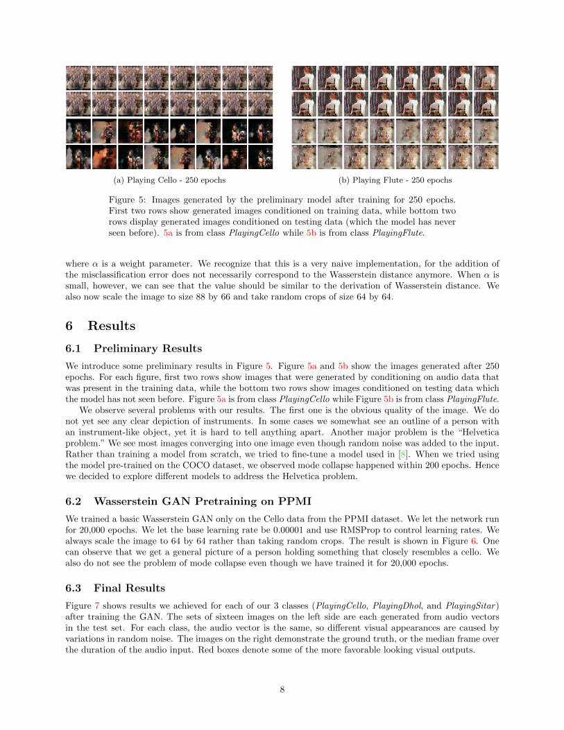
(a) Playing Cello - 250 epochs (b) Playing Flute - 250 epochs

Figure 5: Images generated by the preliminary model after training for 250 epochs.First two rows show generated images conditioned on training data, while bottom tworows display generated images conditioned on testing data (which the model has neverseen before). 5a is from class PlayingCello while 5b is from class PlayingFlute.

where α is a weight parameter. We recognize that this is a very naive implementation, for the addition ofthe misclassification error does not necessarily correspond to the Wasserstein distance anymore. When α issmall, however, we can see that the value should be similar to the derivation of Wasserstein distance. Wealso now scale the image to size 88 by 66 and take random crops of size 64 by 64.

6 Results

6.1 Preliminary Results

We introduce some preliminary results in Figure 5. Figure 5a and 5b show the images generated after 250epochs. For each figure, first two rows show images that were generated by conditioning on audio data thatwas present in the training data, while the bottom two rows show images conditioned on testing data whichthe model has not seen before. Figure 5a is from class PlayingCello while Figure 5b is from class PlayingFlute.

We observe several problems with our results. The first one is the obvious quality of the image. We donot yet see any clear depiction of instruments. In some cases we somewhat see an outline of a person withan instrument-like object, yet it is hard to tell anything apart. Another major problem is the “Helveticaproblem.” We see most images converging into one image even though random noise was added to the input.Rather than training a model from scratch, we tried to fine-tune a model used in [8]. When we tried usingthe model pre-trained on the COCO dataset, we observed mode collapse happened within 200 epochs. Hencewe decided to explore different models to address the Helvetica problem.

6.2 Wasserstein GAN Pretraining on PPMI

We trained a basic Wasserstein GAN only on the Cello data from the PPMI dataset. We let the network runfor 20,000 epochs. We let the base learning rate be 0.00001 and use RMSProp to control learning rates. Wealways scale the image to 64 by 64 rather than taking random crops. The result is shown in Figure 6. Onecan observe that we get a general picture of a person holding something that closely resembles a cello. Wealso do not see the problem of mode collapse even though we have trained it for 20,000 epochs.

6.3 Final Results

Figure 7 shows results we achieved for each of our 3 classes (PlayingCello, PlayingDhol, and PlayingSitar)after training the GAN. The sets of sixteen images on the left side are each generated from audio vectorsin the test set. For each class, the audio vector is the same, so different visual appearances are caused byvariations in random noise. The images on the right demonstrate the ground truth, or the median frame overthe duration of the audio input. Red boxes denote some of the more favorable looking visual outputs.

8

Figure 6: Generated samples after training a Wasserstein GAN for 20,000 epochs.

Figure 7: Generated samples from our final model. On the left we have 16 generatedimages per class given a test audio input. The classes are PlayingCello, PlayingDhol,and PlayingSitar, top to bottom. On the right is the actual video frame that matchesthe audio input. Red squares indicate the examples that we consider to be most repre-sentative of the true image.

9

Figure 8: Images produced by our generator conditioned on the sound of a cello. Thetop two rows of samples were generated from one sound (and different random noise),while the bottom two rows were generated from a second sound (and different randomnoise).

We first note that the results shown are perceptually discriminable from the ground truth images. Weconjecture that this failure was largely due to the lack of diverse data available to the model. However, theseresults suggest our generator learned a few useful properties about the training data.

• Low-level features. Many of the generated samples contain the rough outline of the instrumentdepicted within them. The images also seem to sometimes capture the rough silhouette of the personplaying it. This result makes sense since the network has no concept of people or of instruments, andsince people regularly appear with the instrument, it makes sense that they would be included.

• Different appearances for different classes. The GAN succeeded in producing very differentsamples for each of the three classes it was trained on. The color and shapes produced for each classlook visibly different from the ones produced for other classes, which indicates that the generator learnedthat different sounds are associated with different visual outputs.

• Some diversity generated by random noise. For the Dhol and Sitar classes, the images seemto vary by a significant amount - the random noise is not all mapped to the same visual output. Forthe cello class, there is less diversity amongst samples, although we note that the similar colors in theimages are representative of the colors of an actual cello.

6.4 Discussion of Image Diversity

To check if our model produced diverse samples for different audio data, we tested our generator on twoadditional audio samples of a cello. Figure 8 displays the result. We note that compared to our result inFigure 7, the samples vary more, perhaps at the cost of less reliable quality overall. We also observe that thevisual outputs tend to look distinct from each other and very different than the samples of cellos generated inFigure 7. While there is definitely room for improvement in terms of image quality, our model still managesto produce some diversity in output even for audio inputs of the same class.

7 Future Work

The following steps could improve the results of the paper:

10

• Improve data collection or supervision. Our GAN may have faced difficulties in extrapolatingfrom the relatively small number of labeled examples. We conjecture that with more labeled data, themodel would be able to better interpolate across the space of plausible images. We also think thatbetter quality data (in which, perhaps, background was removed) might increase the quality of images,since less effort is devoted to generating the background.

• Improve the Wasserstein GAN. As mentioned in Section 5.1, [6] addresses the problem of enforcingLipschitz constraint by penalizing the norm of the gradient of the critic rather than clipping the weights.Therefore, a network trained with this model might yield better results. Moreover, [3] discusses in depththe theoretical results for developing a loss function for multi-label setting, and may be studied morefor more accurate implementation.

• Implement a GAN with an attention module. With a dataset that has dense semantic labeling(of foreground or background), it might be possible to train a generator that produces an image andsemantic labels. The discriminator is then trained on whether pixels in the foreground were from thetraining set or the generator. This setup would force the generator to produce images with realisticshapes and textures, and it may also ease the learning problem of generating complicated backgrounds.

11

References

[1] Arjovsky, M., Chintala, S., and Bottou, L. (2017). Wasserstein GAN. arXiv:1701.07875[stat.ML].

[2] Bao, J., Chen, D., Wen, F., Li, H., and Hua, G. (2017). CVAE-GAN: Fine-Grained Image Generationthrough Asymmetric Training. arXiv:1703.10155 [cs.CV].

[3] Frogner, C., Zhang, C., Mobahi, H., Araya-Polo, M., and Poggio, T. (2015). Learning with a WassersteinLoss. Advanced in Neural Information Processing Systems 28.

[4] Goodfellow, I., Pouget-Abadie, J., Mirza, M., Xu B., Warde-Farley D., Ozair S., Courville A., and BengioY. (2014). Generative Adversarial Networks. In Advances in Neural Information Processing Systems 27.

[5] Gorijala, M., and Dukkipati, A. (2017). Image Generation and Editing with Variational Info GenerativeAdversarial Networks. arXiv:1701.04568 [cs.CV].

[6] Gulrajani, I., Ahmed, F., Arjovsky, M., Dumoulin, V., and Courville, A. (2017). Improved Training ofWasserstein GANs. arXiv:1704.00028[cs.LG].

[7] Phan, H., Koch, P., Katzberg, F., Maass, M., Mazur, R., and Mertins, A. (2017). Audio Scene Classifi-cation with Deep Recurrent Neural Networks. arXiv:1703.04770[cs.SD].

[8] Reed, S., Akata, Z., Yan, X., Logeswaran, L., Schiele, B., and Lee, H. (2016). Generative adversarial textto image synthesis. In Proceedings of The 33rd International Conference on Machine Learning.

[9] Soomro, K., Zamir, A. and Shah, M. (2012). UCF101: A Dataset of 101 Human Action Classes FromVideos in The Wild. CRCV-TR-12-01.

[10] Takahashi, N., Gygli, M., and Gool, L. V. (2017). AENet: Learning Deep Audio Features for VideoAnalysis. arXiv:1701.00599[cs.MM].

[11] Vinyals, O., Toshev, A., Bengio, S., and Erhan, D. (2015). Show and Tell: A Neural Image CaptionGenerator. In the Conference on Computer Vision and Pattern Recognition.

[12] Vondrick, C., Aytar, Y., and Torralba, A. (2016). SoundNet: Learning Sound Representations fromUnlabeled Video. In Advances in Neural Information Processing Systems 29.

[13] Yao, B. and Fei-Fei, L. (2010). Grouplet: A Structured Image Representation for Recognizing Humanand Object Interactions. In the Conference on Computer Vision and Pattern Recognition.

[14] Zhu, J., Krahenbuhl, P., Shechtman, E., and Efros, A. A. (2016). Generative Visual Manipulation onthe Natural Image Manifold. In European Conference on Computer Vision, pages 597 - 613.

12