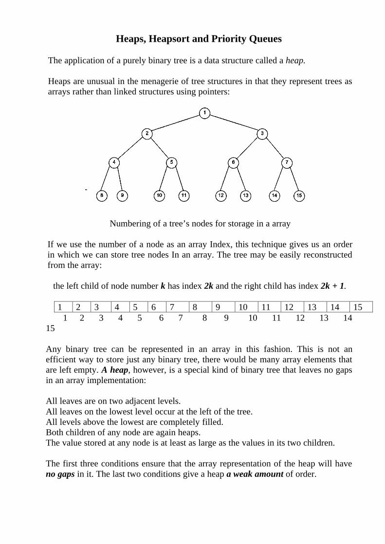
Heaps, Heapsort and Priority Queues

The application of a purely binary tree is a data structure called a heap.

Heaps are unusual in the menagerie of tree structures in that they represent trees asarrays rather than linked structures using pointers:

Numbering of a tree’s nodes for storage in a array

If we use the number of a node as an array Index, this technique gives us an orderin which we can store tree nodes In an array. The tree may be easily reconstructedfrom the array:

the left child of node number k has index 2k and the right child has index 2k + 1.

1 2 3 4 5 6 7 8 9 10 11 12 13 14 15 1 2 3 4 5 6 7 8 9 10 11 12 13 1415

Any binary tree can be represented in an array in this fashion. This is not anefficient way to store just any binary tree, there would be many array elements thatare left empty. A heap, however, is a special kind of binary tree that leaves no gapsin an array implementation:

All leaves are on two adjacent levels.All leaves on the lowest level occur at the left of the tree.All levels above the lowest are completely filled.Both children of any node are again heaps.The value stored at any node is at least as large as the values in its two children.

The first three conditions ensure that the array representation of the heap will haveno gaps in it. The last two conditions give a heap a weak amount of order.

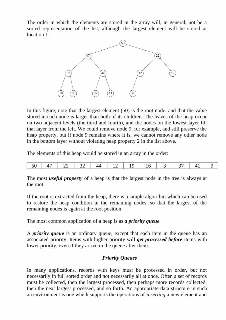
The order in which the elements are stored in the array will, in general, not be asorted representation of the list, although the largest element will be stored atlocation 1.

In this figure, note that the largest element (50) is the root node, and that the valuestored in each node is larger than both of its children. The leaves of the heap occuron two adjacent levels (the third and fourth), and the nodes on the lowest layer fillthat layer from the left. We could remove node 9, for example, and still preserve theheap property, but if node 9 remains where it is, we cannot remove any other nodein the bottom layer without violating heap property 2 in the list above.

The elements of this heap would be stored in an array in the order:

50 47 22 32 44 12 19 16 3 37 41 9

The most useful property of a heap is that the largest node in the tree is always atthe root.

If the root is extracted from the heap, there is a simple algorithm which can be usedto restore the heap condition in the remaining nodes, so that the largest of theremaining nodes is again at the root position.

The most common application of a heap is as a priority queue.

A priority queue is an ordinary queue, except that each item in the queue has anassociated priority. Items with higher priority will get processed before items withlower priority, even if they arrive in the queue after them.

Priority Queues

In many applications, records with keys must be processed in order, but notnecessarily in full sorted order and not necessarily all at once. Often a set of recordsmust be collected, then the largest processed, then perhaps more records collected,then the next largest processed, and so forth. An appropriate data structure in suchan environment is one which supports the operations of inserting a new element and

deleting the largest element. Such a data structure, which can be contrasted withqueues (delete the oldest) and stacks (delete the newest) is called a priority queue.

In fact, the priority queue might be thought of as a generalization of the stack andthe queue (and other simple data structures), since these data structures can beimplemented with priority queues, using appropriate priority assignments.

Applications of priority queues include simulation systems (where the keys mightcorrespond to "event times" which must be processed in order), job scheduling incomputer systems (where the keys might correspond to "priorities" indicating whichusers should be processed first), and numerical computations (where the keys mightbe computational errors, so the largest can be worked on first).

It is useful to be somewhat more precise about how to manipulate a priority queue,since there are several operations we may need to perform on priority queues inorder to maintain them and use them effectively for applications such as thosementioned above. Indeed, the main reason that priority queues are so useful is theirflexibility in allowing a variety of different operations to be efficiently performedon sets of records with keys. We want to build and maintain a data structurecontaining records with numerical keys (priorities) and supporting some of thefollowing operations:

Construct a priority queue from N given items.Insert a new item.Remove the largest item.Replace the largest item with a new item (unless the new item is larger).Change the priority of an item.Delete an arbitrary specified item.Join two priority queues into one large one.

(If records can have duplicate keys, we take "largest" to mean "any record with thelargest key value.")

Different implementations of priority queues involve different performancecharacteristics for the various operations to be performed, leading to cost tradeoffs.Indeed, performance differences are really the only differences that can arise in theabstract data structure concept.

First, we'll illustrate this point by discussing a few elementary data structures forimplementing priority queues. Next, we'll examine a more advanced data structureand then show how the various operations can be implemented efficiently using thisdata structure. We'll then look at an important sorting algorithm that followsnaturally from these implementations.

Any priority queue algorithm can be turned into a sorting algorithm by repeatedlyusing insert to build a priority queue containing all the items to be sorted, thenrepeatedly using remove to empty the priority queue, receiving the items in reverseorder. Using a priority queue represented as an unordered list in this waycorresponds to selection sort; using the ordered list corresponds to insertion sort.

Although heaps are fairly sloppy in keeping their members in strict order, they arevery good at rinding the maximum member and bringing it to the top of the heap.

Constructing a Heap

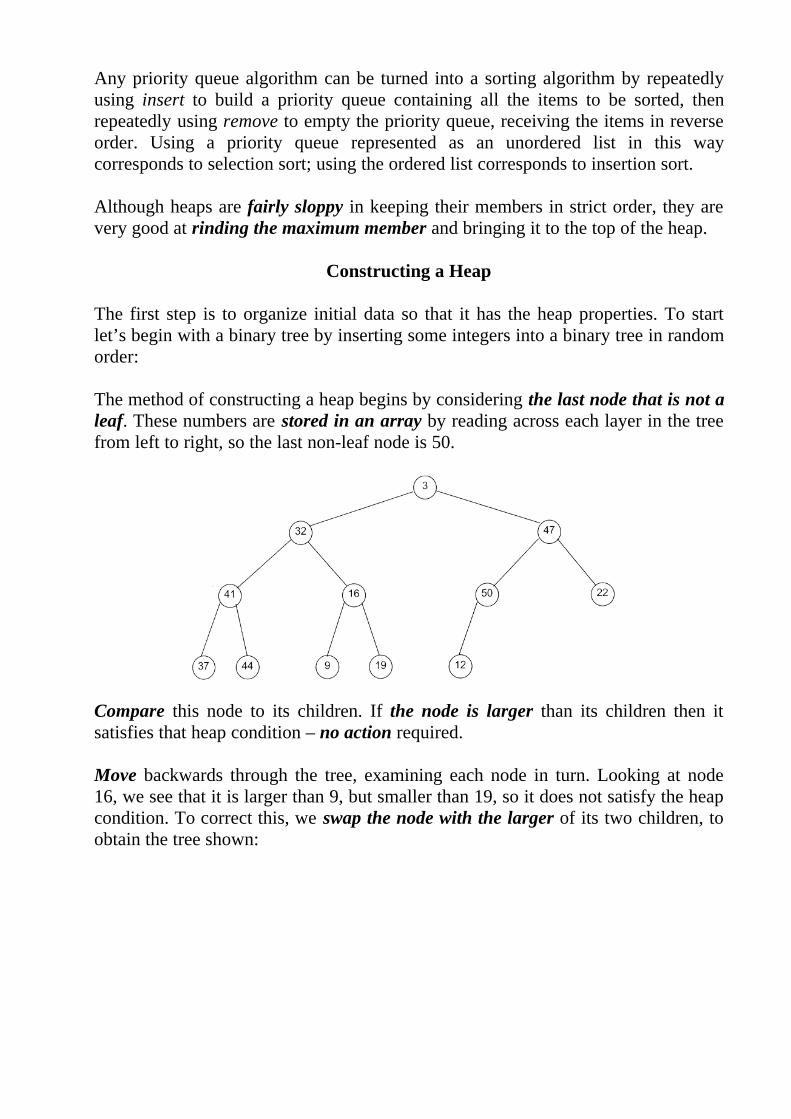
The first step is to organize initial data so that it has the heap properties. To startlet’s begin with a binary tree by inserting some integers into a binary tree in randomorder:

The method of constructing a heap begins by considering the last node that is not aleaf. These numbers are stored in an array by reading across each layer in the treefrom left to right, so the last non-leaf node is 50.

Compare this node to its children. If the node is larger than its children then itsatisfies that heap condition – no action required.

Move backwards through the tree, examining each node in turn. Looking at node16, we see that it is larger than 9, but smaller than 19, so it does not satisfy the heapcondition. To correct this, we swap the node with the larger of its two children, toobtain the tree shown:

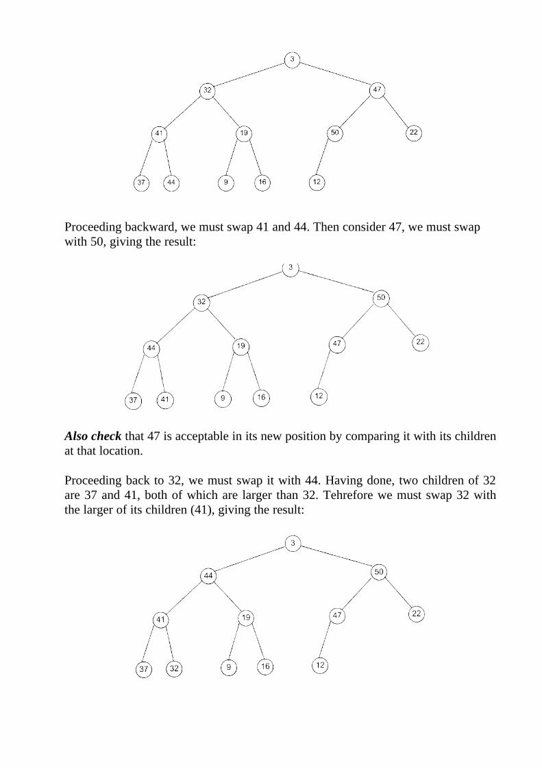
Proceeding backward, we must swap 41 and 44. Then consider 47, we must swapwith 50, giving the result:

Also check that 47 is acceptable in its new position by comparing it with its childrenat that location.

Proceeding back to 32, we must swap it with 44. Having done, two children of 32are 37 and 41, both of which are larger than 32. Tehrefore we must swap 32 withthe larger of its children (41), giving the result:

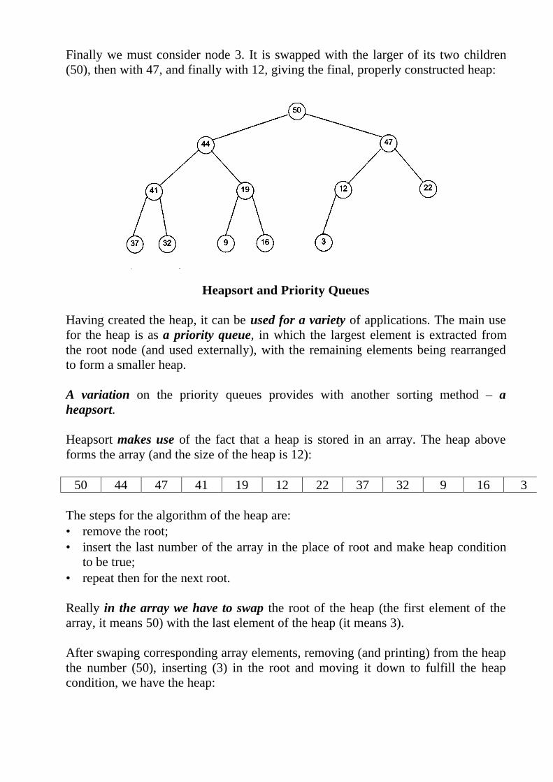
Finally we must consider node 3. It is swapped with the larger of its two children(50), then with 47, and finally with 12, giving the final, properly constructed heap:

Heapsort and Priority Queues

Having created the heap, it can be used for a variety of applications. The main usefor the heap is as a priority queue, in which the largest element is extracted fromthe root node (and used externally), with the remaining elements being rearrangedto form a smaller heap.

A variation on the priority queues provides with another sorting method – aheapsort.

Heapsort makes use of the fact that a heap is stored in an array. The heap aboveforms the array (and the size of the heap is 12):

50 44 47 41 19 12 22 37 32 9 16 3

The steps for the algorithm of the heap are:• remove the root;• insert the last number of the array in the place of root and make heap condition

to be true;• repeat then for the next root.

Really in the array we have to swap the root of the heap (the first element of thearray, it means 50) with the last element of the heap (it means 3).

After swaping corresponding array elements, removing (and printing) from the heapthe number (50), inserting (3) in the root and moving it down to fulfill the heapcondition, we have the heap:

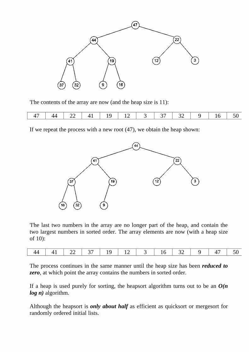
'I'he contents of the array are now (and the heap size is 11):

47 44 22 41 19 12 3 37 32 9 16 50

If we repeat the process with a new root (47), we obtain the heap shown:

'I'he last two numbers in the array are no longer part of the heap, and contain thetwo largest numbers in sorted order. The array elements are now (with a heap sizeof 10):

44 41 22 37 19 12 3 16 32 9 47 50

The process continues in the same manner until the heap size has been reduced tozero, at which point the array contains the numbers in sorted order.

If a heap is used purely for sorting, the heapsort algorithm turns out to be an O(nlog n) algorithm.

Although the heapsort is only about half as efficient as quicksort or mergesort forrandomly ordered initial lists.

The same technique can be used to implement a priority queue. Rather than carrythe sorting process through to the bitter end, the root node can be extracted (whichis the item with highest priority) and rearrange the tree, so that the remaining nodesform a heap with one less element. We need not process the data any further untilthe next request comes in for an item from the priority queue.

A heap is an efficient way of implementing a priority queue since the maximumnumber of nodes that need to be considered to restore the heap property when theroot is extracted is about twice the depth of the tree. The number of comparisons isaround 2 log N

Algorithms on Heaps

The priority queue algorithms on heaps all work by first making a simple structuralmodification which could violate the heap condition, then traveling through theheap modifying it to ensure that the heap condition is satisfied everywhere.

Some of the algorithms travel through the heap from bottom to top, others from topto bottom. In all of the algorithms,,we'll assume that the records are one-wordinteger keys stored in an array a of some maximum size, with the current size of theheap kept in an integer N. Note that N is as much a part of the definition of the heapas the keys and records themselves.

To be able to build a heap, it is necessary first to implement the insert operation.Since this operation will increase the size of the heap by one, N must beincremented. Then the record to be inserted is put into a [N], but this may violatethe heap property. If the heap property is violated (the new node is greater than itsparent), then the violation can be fixed by exchanging the new node with its parent.This may, in turn, cause a violation, and thus can be fixed in the same way.

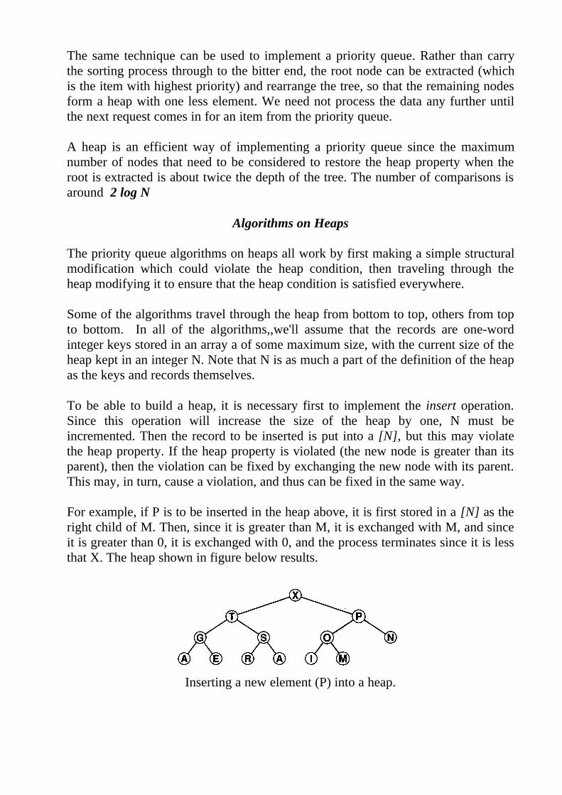
For example, if P is to be inserted in the heap above, it is first stored in a [N] as theright child of M. Then, since it is greater than M, it is exchanged with M, and sinceit is greater than 0, it is exchanged with 0, and the process terminates since it is lessthat X. The heap shown in figure below results.

Inserting a new element (P) into a heap.

The code for this method is straightforward. In the following implementation, insertadds a new item to a [N], then calls upheap (N) to fix the heap condition violation atN:

procedure upheap(k: integer);var v: integer;beginv:=a[k]; a[O]:=maxint;while a [k div 2 1 < =v dobegin a [k ]:=a [k div 2 1; k:=k div 2 end;a [k ]:=vend;

procedure insert(v: integer);beginN:=N+l; a[N]:=v;upheap (N)end;

If k div 2 were replaced by k-1 everywhere in this program, we would have inessence one step of insertion sort (implementing a priority queue with an orderedlist); here, instead, we are "inserting" the new key along the path from N to the root.As with insertion sort, it is not necessary to do a full exchange within the loop,because v is always involved in the exchanges.

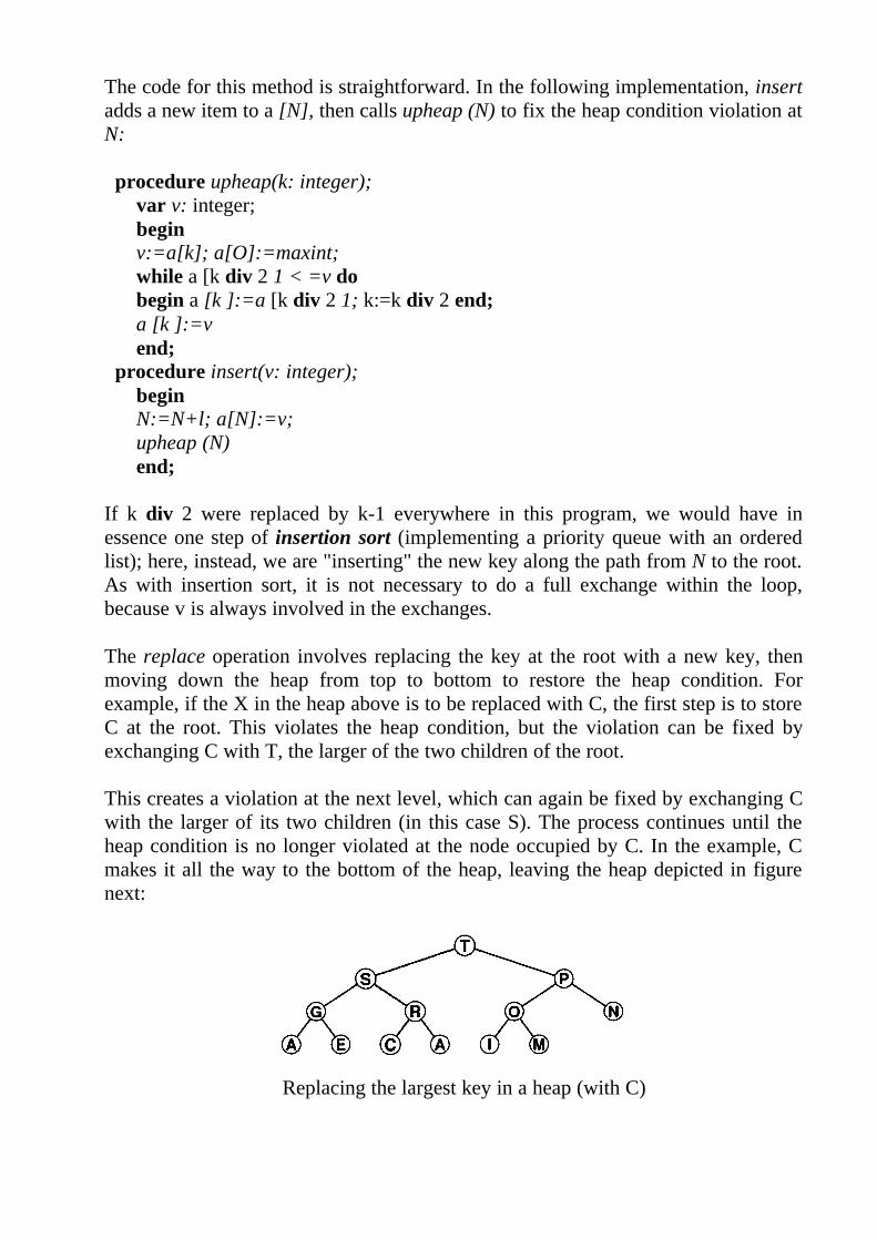
The replace operation involves replacing the key at the root with a new key, thenmoving down the heap from top to bottom to restore the heap condition. Forexample, if the X in the heap above is to be replaced with C, the first step is to storeC at the root. This violates the heap condition, but the violation can be fixed byexchanging C with T, the larger of the two children of the root.

This creates a violation at the next level, which can again be fixed by exchanging Cwith the larger of its two children (in this case S). The process continues until theheap condition is no longer violated at the node occupied by C. In the example, Cmakes it all the way to the bottom of the heap, leaving the heap depicted in figurenext:

Replacing the largest key in a heap (with C)

The "remove the largest" operation involves almost the same process. Since theheap will be one element smaller after the operation, it is necessary to decrement N,leaving no place for the element that was stored in the last position. But the largestelement (which is in a [ 1 ]) is to be removed, so the remove operation amounts to areplace, using the element that was in a [N]. The heap shown in figure is the resultof removing the T from the heap in figure preceeding by replacing it with the M,then moving down, promoting the larger of the two children, until reaching a nodewith both children smaller than M.

The implementation of both of these operations is centered around the process offixing up a heap which satisfies the heap condition everywhere except possibly atthe root. If the key at the root is too small, it must be moved down the heap withoutviolating the heap property at any of the nodes touched. It turns out that the sameoperation can be used to fix up the heap after the value in any position is lowered.It may be implemented as follows:

label 0;var i.i. v: integer;beginv:=a [kwhile k<=N div 2 do

beginj:=k+k;if j<N then if a Ul <a U+l if v > =a U ] then goto 0; a[kl:=aU]; k:=j; end;

0: a[k]:=vend;

procedure downheap(k: integer);label 0;var i,j. v: integer;beginv: =a [k 1;

while k<=N div 2 dobeginj:=k+k;if j<N then if a Ul <a U+l I then j:=j+l;if v >=a [ j ] then goto 0;a[kl:=aU]; k:=j;end;

0: a[k]:=vend;

This procedure moves down the heap, exchanging the node at position k with thelarger of its two children if necessary and stopping when the node at k is larger thanboth children or the bottom is reached. (Note that it is possible for the node at k to

have only one child: this case must be treated properly!) As above, a full exchangeis not needed because v is always involved in the exchanges. The inner loop in thisprogram is an example of a loop which really has two distinct exits: one for the casethat the bottom of the heap is hit (as in the first example above), and another for thecase that the heap condition is satisfied somewhere in the interior of the heap. Thegoto could be avoided, with some work, and at some expense in clarity.

Now the implementation of the remove operation is a direct application of thisprocedure:

function remove: integer;beginremove:=a [1a[l]:=a[N]; N:=N-1;downheap (1);end;

The return value is set from a [I] and then the element from a [N] is put into a [1]and the size of the heap decremented, leaving only a call to downheap to fix up theheap condition everywhere.

The implementation of the replace operation is only slightly more complicated:

function replace(v: integer):integer;begin

a[0]:=v;downheap (0);replace: =a [0]end;

This code uses a [0] in an artificial way: its children are 0 (itself) and 1, so if v islarger than the largest element in the heap, the heap is not touched; otherwise v isput into the heap and a [I] is returned.

The delete operation for an arbitrary element from the heap and the changeoperation can also be implemented by using a simple combination of the methodsabove. For example, if the priority of the element at position k is raised, thenupheap(k) can be called, and if it is lowered then downheap(k) does the job.

Property 1 All of the basic operations insert, remove, replace, (downheap andupheap), delete, and change require less than 2 Ig N comparisons when performedon a heap of N elements.

All these operations involve moving along a path between the root and the bottomof the heap, which includes no more than IgN elements for a heap of size N. The

factor of two comes from downheap, which makes two comparisons in its innerloop; the other operations require only IgN comparisons.

Note carefully that thejoin operation is not included on this list. Doing thisoperation efficiently seems to require a much more sophisticated data structure. Onthe other hand, in many applications, one would expect this operation to be requiredmuch less frequently than the others.

Indirect Heaps

For many applications of priority queues, we don't want the records moved aroundat all. Instead, we want the priority queue routine not to return values but to tell uswhich of the records is the largest, etc. This is akin to the "indirect sort" or the"pointer sort". Modifying the above programs to work in this way isstraightforward, though sometimes confusing. It will be worthwhile to examine thisin more detail here because it is so convenient to use heaps in this way.

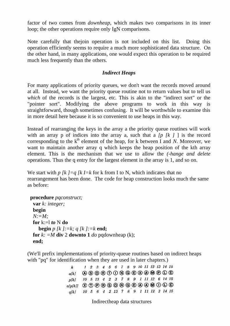
Instead of rearranging the keys in the array a the priority queue routines will workwith an array p of indices into the array a, such that a [p [k ] ] is the recordcorresponding to the kth element of the heap, for k between I and N. Moreover, wewant to maintain another array q which keeps the heap position of the kth arrayelement. This is the mechanism that we use to allow the (-hange and deleteoperations. Thus the q entry for the largest element in the array is 1, and so on.

We start with p [k ]=q [k I=k for k from I to N, which indicates that norearrangement has been done. The code for heap construction looks much the sameas before:

procedure pqconstruct;var k: integer;beginN:=M;for k:=l to N do

begin p [k ]:=k; q [k ]:=k end;for k: =M div 2 downto 1 do pqdownheap (k);end;

(We'll prefix implementations of priority-queue routines based on indirect heapswith "pq" for identification when they are used in later chapters.)

Indirectheap data structures

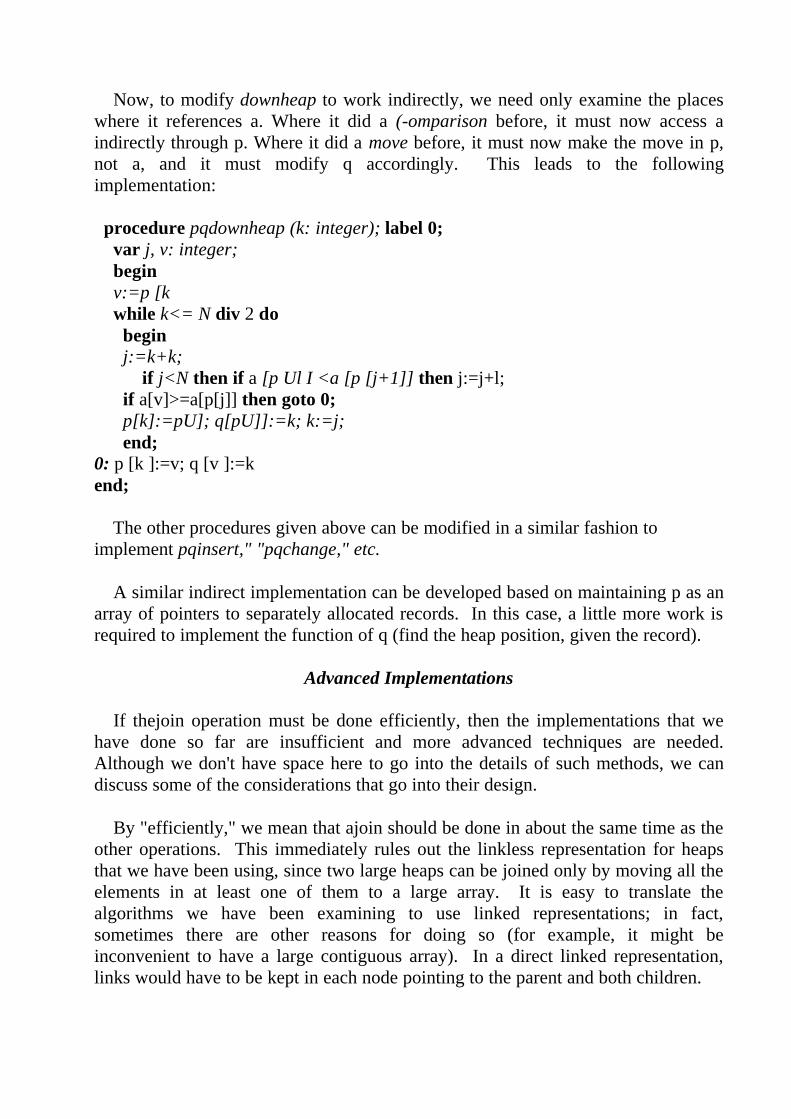
Now, to modify downheap to work indirectly, we need only examine the placeswhere it references a. Where it did a (-omparison before, it must now access aindirectly through p. Where it did a move before, it must now make the move in p,not a, and it must modify q accordingly. This leads to the followingimplementation:

procedure pqdownheap (k: integer); label 0;var j, v: integer;beginv:=p [kwhile k<= N div 2 do

beginj:=k+k;

if j<N then if a [p Ul I <a [p [j+1]] then j:=j+l;if a[v]>=a[p[j]] then goto 0;p[k]:=pU]; q[pU]]:=k; k:=j;end;

0: p [k ]:=v; q [v ]:=kend;

The other procedures given above can be modified in a similar fashion toimplement pqinsert," "pqchange," etc.

A similar indirect implementation can be developed based on maintaining p as anarray of pointers to separately allocated records. In this case, a little more work isrequired to implement the function of q (find the heap position, given the record).

Advanced Implementations

If thejoin operation must be done efficiently, then the implementations that wehave done so far are insufficient and more advanced techniques are needed.Although we don't have space here to go into the details of such methods, we candiscuss some of the considerations that go into their design.

By "efficiently," we mean that ajoin should be done in about the same time as theother operations. This immediately rules out the linkless representation for heapsthat we have been using, since two large heaps can be joined only by moving all theelements in at least one of them to a large array. It is easy to translate thealgorithms we have been examining to use linked representations; in fact,sometimes there are other reasons for doing so (for example, it might beinconvenient to have a large contiguous array). In a direct linked representation,links would have to be kept in each node pointing to the parent and both children.

It turns out that the heap condition itself seems to be too strong to allow efficientimplementation of thejoin operation. The advanced data structures designed tosolve this problem all weaken either the heap or the balance condition in order togain the flexibility needed for thejoin. These structures allow all the operations tobe completed in logarithmic time.

B-Trees

Multiway Search Trees

The trees that we have considered so far have all been binary (almost) trees: eachnode can have no more than two children. Since the main factor in determining theefficiency of a tree is its depth, it is natural to ask if the efficiency can be improvedby allowing nodes to have more than two children. It is fairly obvious that if weallow more than one item to be stored at each node of a tree, the depth of the treewill be less.

In general, however, any attempt to increase the efficiency of a tree by allowingmore data to be stored in each node is compriomised by the extra work required tolocate an item within the node. To be sure that we are getting any benefit out of amultiway search tree, we should do some calculations or simulations for typicaldata sets and compare the results with an ordinary binary tree.

But for the data stored on other media, in external memory, the access time is manytimes slower than for primary memory. We would like some form of data storagethat minimizes the number of times such accesses must be made.

We therefore want a way of searching through the data on disk while satisfying twoconditions:• the amount of data read by each disk access should be close to the page (block,

cluster) size;• the number of disk accesses should be minimized.

If we use a binary tree to store the data on disk, we must access each item of dataseparately since we do not know in which direction we should branch until we havecompared the node's value with the item for which we are searching. This isinefficient in terms of disk accesses.

The main solution to this problem is to use a multiway search tree in which tostore the data, where the maximum amount of data that can be stored at each node isclose to (but does not exceed) the block size for a single disk read operation. Wecan then load a single node (containing many data items) into RAM and process thisdata entirely in RAM.

Although there will be some overhead in the sorting and searching operationsrequired to insert and search for data within each node, all of these operations aredone exclusively in RAM and are therefore much faster than accessing the hard diskor other external medium.

The B -Tree: a Balanced Multiway Search Tree

It is customary to classify a multiway tree by the maximum number of branches ateach node, rather than the maximum number of items which may be stored at eachnode. If we use a multiway search tree with M possible branches at each node, thenwe can store up to M - 1 data items at each node.Since multiway trees are primarily used in databases, the data that are stored areusually of a fairly complex type.

In each node of a multiway search tree, we may have up to M - 1 keys labeled

To get the greatest efficiency gain out of a multiway search tree, we need to ensurethat most of the nodes contain as much data as possible, and that the tree is asbalanced as possible. There are several algorithms which approach this problemfrom various angles, but the most popular method is the B-tree:

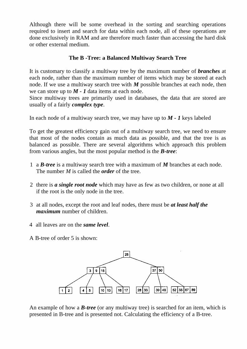
1 a B-tree is a multiway search tree with a maximum of M branches at each node.The number M is called the order of the tree.

2 there is a single root node which may have as few as two children, or none at allif the root is the only node in the tree.

3 at all nodes, except the root and leaf nodes, there must be at least half themaximum number of children.

4 all leaves are on the same level.

A B-tree of order 5 is shown:

An example of how a B-tree (or any multiway tree) is searched for an item, which ispresented in B-tree and is presented not. Calculating the efficiency of a B-tree.

Constructing a B-Tree

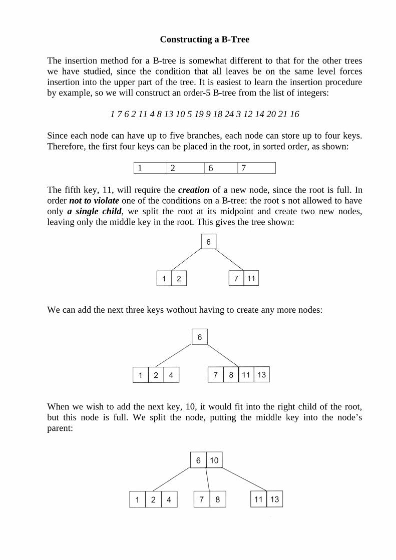
The insertion method for a B-tree is somewhat different to that for the other treeswe have studied, since the condition that all leaves be on the same level forcesinsertion into the upper part of the tree. It is easiest to learn the insertion procedureby example, so we will construct an order-5 B-tree from the list of integers:

1 7 6 2 11 4 8 13 10 5 19 9 18 24 3 12 14 20 21 16

Since each node can have up to five branches, each node can store up to four keys.Therefore, the first four keys can be placed in the root, in sorted order, as shown:

1 2 6 7

The fifth key, 11, will require the creation of a new node, since the root is full. Inorder not to violate one of the conditions on a B-tree: the root s not allowed to haveonly a single child, we split the root at its midpoint and create two new nodes,leaving only the middle key in the root. This gives the tree shown:

We can add the next three keys wothout having to create any more nodes:

When we wish to add the next key, 10, it would fit into the right child of the root,but this node is full. We split the node, putting the middle key into the node’sparent:

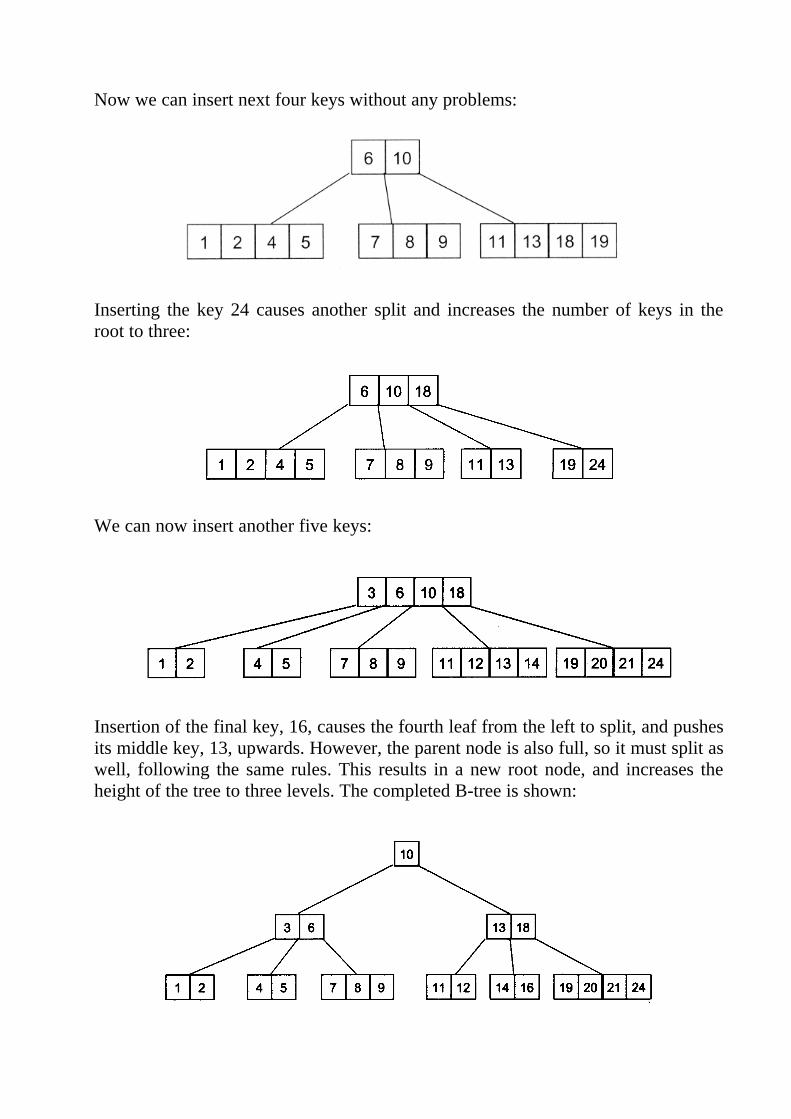
Now we can insert next four keys without any problems:

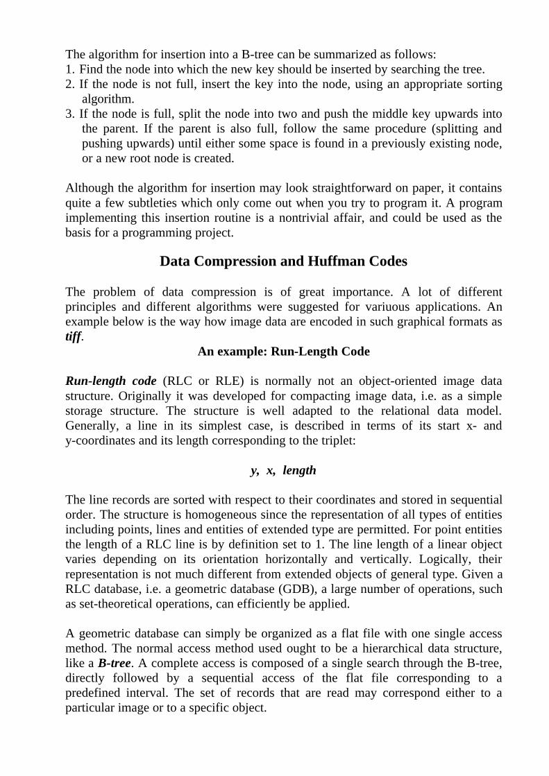
Inserting the key 24 causes another split and increases the number of keys in theroot to three:

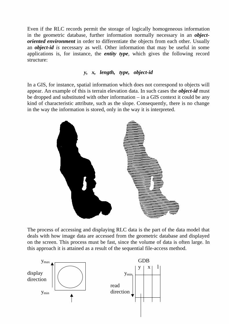
We can now insert another five keys:

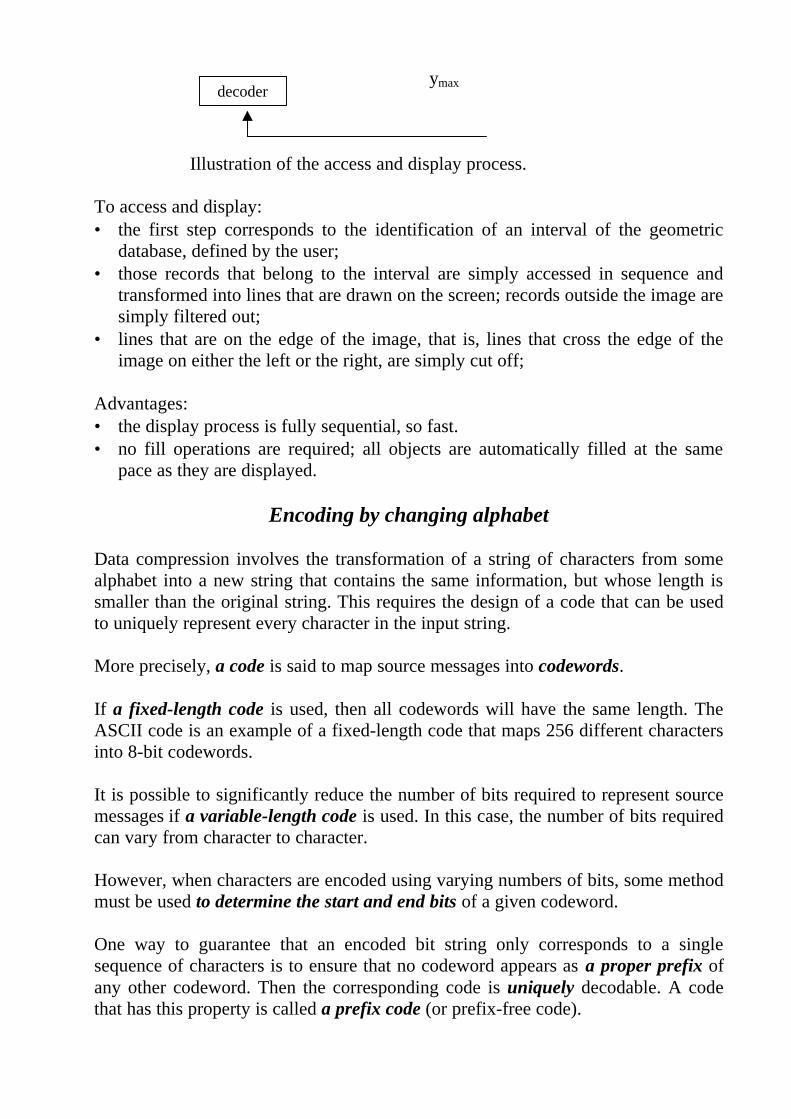
Insertion of the final key, 16, causes the fourth leaf from the left to split, and pushesits middle key, 13, upwards. However, the parent node is also full, so it must split aswell, following the same rules. This results in a new root node, and increases theheight of the tree to three levels. The completed B-tree is shown:

The algorithm for insertion into a B-tree can be summarized as follows:1. Find the node into which the new key should be inserted by searching the tree.2. If the node is not full, insert the key into the node, using an appropriate sorting

algorithm.3. If the node is full, split the node into two and push the middle key upwards into

the parent. If the parent is also full, follow the same procedure (splitting andpushing upwards) until either some space is found in a previously existing node,or a new root node is created.

Although the algorithm for insertion may look straightforward on paper, it containsquite a few subtleties which only come out when you try to program it. A programimplementing this insertion routine is a nontrivial affair, and could be used as thebasis for a programming project.

Data Compression and Huffman Codes

The problem of data compression is of great importance. A lot of differentprinciples and different algorithms were suggested for variuous applications. Anexample below is the way how image data are encoded in such graphical formats astiff.

An example: Run-Length Code

Run-length code (RLC or RLE) is normally not an object-oriented image datastructure. Originally it was developed for compacting image data, i.e. as a simplestorage structure. The structure is well adapted to the relational data model.Generally, a line in its simplest case, is described in terms of its start x- andy-coordinates and its length corresponding to the triplet:

y, x, length

The line records are sorted with respect to their coordinates and stored in sequentialorder. The structure is homogeneous since the representation of all types of entitiesincluding points, lines and entities of extended type are permitted. For point entitiesthe length of a RLC line is by definition set to 1. The line length of a linear objectvaries depending on its orientation horizontally and vertically. Logically, theirrepresentation is not much different from extended objects of general type. Given aRLC database, i.e. a geometric database (GDB), a large number of operations, suchas set-theoretical operations, can efficiently be applied.

A geometric database can simply be organized as a flat file with one single accessmethod. The normal access method used ought to be a hierarchical data structure,like a B-tree. A complete access is composed of a single search through the B-tree,directly followed by a sequential access of the flat file corresponding to apredefined interval. The set of records that are read may correspond either to aparticular image or to a specific object.

Even if the RLC records permit the storage of logically homogeneous informationin the geometric database, further information normally necessary in an object-oriented environment in order to differentiate the objects from each other. Usuallyan object-id is necessary as well. Other information that may be useful in someapplications is, for instance, the entity type, which gives the following recordstructure:

y, x, length, type, object-id

In a GIS, for instance, spatial information which does not correspond to objects willappear. An example of this is terrain elevation data. In such cases the object-id mustbe dropped and substituted with other information – in a GIS context it could be anykind of characteristic attribute, such as the slope. Consequently, there is no changein the way the information is stored, only in the way it is interpreted.

The process of accessing and displaying RLC data is the part of the data model thatdeals with how image data are accessed from the geometric database and displayedon the screen. This process must be fast, since the volume of data is often large. Inthis approach it is attained as a result of the sequential file-access method.

ymax GDBy x l

display ymin

directionread

ymin direction

ymax

Illustration of the access and display process.

To access and display:• the first step corresponds to the identification of an interval of the geometric

database, defined by the user;• those records that belong to the interval are simply accessed in sequence and

transformed into lines that are drawn on the screen; records outside the image aresimply filtered out;

• lines that are on the edge of the image, that is, lines that cross the edge of theimage on either the left or the right, are simply cut off;

Advantages:• the display process is fully sequential, so fast.• no fill operations are required; all objects are automatically filled at the same

pace as they are displayed.

Encoding by changing alphabet

Data compression involves the transformation of a string of characters from somealphabet into a new string that contains the same information, but whose length issmaller than the original string. This requires the design of a code that can be usedto uniquely represent every character in the input string.

More precisely, a code is said to map source messages into codewords.

If a fixed-length code is used, then all codewords will have the same length. TheASCII code is an example of a fixed-length code that maps 256 different charactersinto 8-bit codewords.

It is possible to significantly reduce the number of bits required to represent sourcemessages if a variable-length code is used. In this case, the number of bits requiredcan vary from character to character.

However, when characters are encoded using varying numbers of bits, some methodmust be used to determine the start and end bits of a given codeword.

One way to guarantee that an encoded bit string only corresponds to a singlesequence of characters is to ensure that no codeword appears as a proper prefix ofany other codeword. Then the corresponding code is uniquely decodable. A codethat has this property is called a prefix code (or prefix-free code).

decoder

Not only are prefix codes uniquely decodable, they also have the desirable propertyof being instantaneously decodable. This means that a codeword in a codedmessage can be decoded without having to look ahead to other codewords in themessage.

A technique that can be used to construct optimal prefix codes will be presented onthe name of Huffman codes.

This method of data compression involves calculating the frequencies of all thecharacters in a given message before the message is stored or transmitted. Next, avariable-length prefix code is constructed, with more frequently occurringcharacters encoded with shorter codewords, and less frequently occurring charactersencoded with longer codewords.

The code must be included with the encoded message; otherwise the message couldnot be decoded.

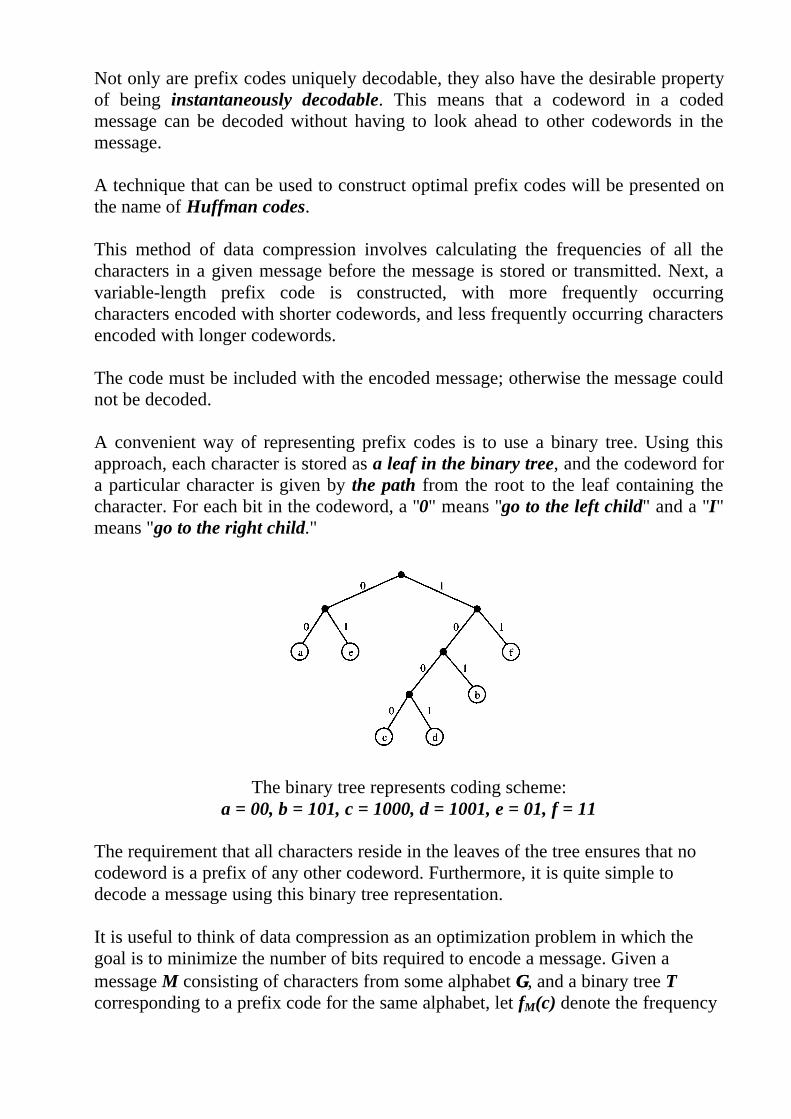
A convenient way of representing prefix codes is to use a binary tree. Using thisapproach, each character is stored as a leaf in the binary tree, and the codeword fora particular character is given by the path from the root to the leaf containing thecharacter. For each bit in the codeword, a "0" means "go to the left child" and a "I"means "go to the right child."

The binary tree represents coding scheme:a = 00, b = 101, c = 1000, d = 1001, e = 01, f = 11

The requirement that all characters reside in the leaves of the tree ensures that nocodeword is a prefix of any other codeword. Furthermore, it is quite simple todecode a message using this binary tree representation.

It is useful to think of data compression as an optimization problem in which thegoal is to minimize the number of bits required to encode a message. Given amessage M consisting of characters from some alphabet ΓΓ, and a binary tree Tcorresponding to a prefix code for the same alphabet, let fM(c) denote the frequency

of character c in M and dT (c) the depth of the leaf that stores c in T. Then the cost(i.e., the number of bits required) to encode M using T is

Minimization of this cost function will yield an optimal prefix code for M. Thebinary tree that represents this optimal prefix code is an optimal tree.

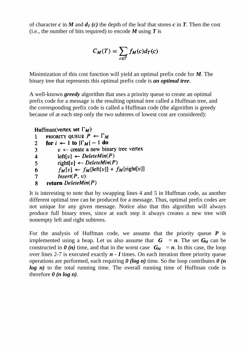
A well-known greedy algorithm that uses a priority queue to create an optimalprefix code for a message is the resulting optimal tree called a Huffman tree, andthe corresponding prefix code is called a Huffman code (the algorithm is greedybecause of at each step only the two subtrees of lowest cost are considered):

It is interesting to note that by swapping lines 4 and 5 in Huffman code, aa anotherdifferent optimal tree can be produced for a message. Thus, optimal prefix codes arenot unique for any given message. Notice also that this algorithm will alwaysproduce full binary trees, since at each step it always creates a new tree withnonempty left and right subtrees.

For the analysis of Huffman code, we assume that the priority queue P isirnplemented using a heap. Let us also assume that ΓΓ = n. The set ΓΓM can beconstructed in 0 (n) time, and that in the worst case ΓΓM = n. In this case, the loopover lines 2-7 is executed exactly n - I times. On each iteration three priority queueoperations are performed, each requiring 0 (log n) time. So the loop contributes 0 (nlog n) to the total running time. The overall running time of Huffman code istherefore 0 (n log n).

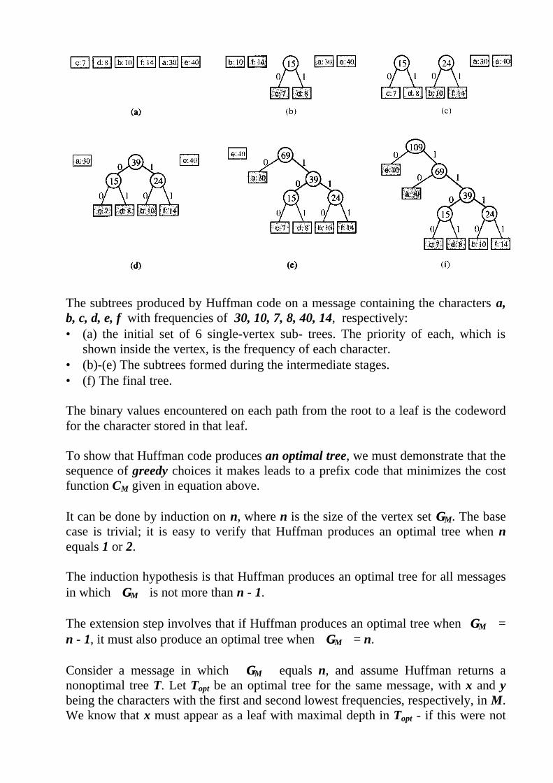
The subtrees produced by Huffman code on a message containing the characters a,b, c, d, e, f with frequencies of 30, 10, 7, 8, 40, 14, respectively:• (a) the initial set of 6 single-vertex sub- trees. The priority of each, which is

shown inside the vertex, is the frequency of each character.• (b)-(e) The subtrees formed during the intermediate stages.• (f) The final tree.

The binary values encountered on each path from the root to a leaf is the codewordfor the character stored in that leaf.

To show that Huffman code produces an optimal tree, we must demonstrate that thesequence of greedy choices it makes leads to a prefix code that minimizes the costfunction CM given in equation above.

It can be done by induction on n, where n is the size of the vertex set ΓΓM. The basecase is trivial; it is easy to verify that Huffman produces an optimal tree when nequals 1 or 2.

The induction hypothesis is that Huffman produces an optimal tree for all messagesin which ΓΓM is not more than n - 1.

The extension step involves that if Huffman produces an optimal tree when ΓΓM =n - 1, it must also produce an optimal tree when ΓΓM = n.

Consider a message in which ΓΓM equals n, and assume Huffman returns anonoptimal tree T. Let Topt be an optimal tree for the same message, with x and ybeing the characters with the first and second lowest frequencies, respectively, in M.We know that x must appear as a leaf with maximal depth in Topt - if this were not

the case, we could exchange this leaf with the lowest leaf in the tree, therebydecreasing CM and contradicting the optimality of Topt.

Moreover, we can always exchange vertices in Topt, without affecting CM, so thatthe vertices storing x and y become siblings. These two vertices must also appear assiblings in T - they are paired together on the first iteration of Huffman. Nowconsider the two trees T' and T'opt , produced by replacing these two siblings andtheir parent with a single vertex containing a new character z whose frequencyequals fM[x] + fM[y].

Note that Huffman would produce T' on the message M' obtained by replacing alloccurrences of x and y in M with z. Except for x and y, the depth of every characterin these new trees is the same as it was in the old trees. Furthermore, in both T' andT'opt the new character z appears one level higher than both x and y did in T andTopt, respectively. Thus, we have that

Since we have assumed that CM(Topt) < CM(T), it follows that CM (T'opt) < CM

(T'). But T' is a Huffman tree in which ΓΓ = n-1, so this latter inequalitycontradicts our induction hypothesis.