This work is licensed under a

Creative Commons Attribution-NonCommercial-NoDerivatives 4.0 International licence

Newcastle University ePrints - eprint.ncl.ac.uk

Bhattacharjee A, Shin JK, Subramanian C, Swaminathan S. Healthcare

Investment and Income Inequality. Journal of Health Economics 2017

Copyright:

© 2017. This manuscript version is made available under the CC-BY-NC-ND 4.0 license

DOI link to article:

https://doi.org/10.1016/j.jhealeco.2017.08.007

Date deposited:

10/10/2017

Embargo release date:

07 April 2019

1

Healthcare Investment and Income Inequality

Ayona Bhattacharjeea, Jong Kook Shinb, Chetan Subramanianc, Shailender Swaminathand

Abstract

This paper examines how the relative shares of public and private health expenditures impact income inequality. We study a two period overlapping generation’s growth model in which longevity is determined by both private and public health expenditure and human capital is the engine of growth. Increased investment in health, reduces mortality, raises return to education and affects income inequality. In such a framework we show that the cross-section earnings inequality is non-decreasing in the private share of health expenditure. We test this prediction empirically using a variable that proxies for the relative intensity of investments (private versus public) using vaccination data from the National Sample Survey Organization for 76 regions in India in the year 1986-87. We link this with region-specific expenditure inequality data for the period 1987-2012. Our empirical findings, though focused on a specific health investment (vaccines), suggest that an increase in the share of the privately provided health care results in higher inequality.

JEL classification: I14, I15, O11

Keywords: Public and Private Health, Longevity, Income inequality,

Growth

a O.P. Jindal Global Business School, Sonipat-Narela Road, Delhi NCR. Haryana-131001, India

b Newcastle University Business School, 5 Barrack Road, Newcastle upon Tyne, NE1 4SE, U.K

c Department of Economics and Social Sciences, IIM Bangalore, Bannerghatta Road, Bangalore 560076, India

d Public Health Foundation of India, Brown University, Providence, RI, USA

2

1 Introduction

This paper contributes to the growing debate on whether the delivery of health care should

be public or private by examining the interplay between the shares of public and private

health expenditure in an economy and income inequality. Although the total spending on

public and private health care has been rising in most countries, there are considerable

differences in the mixture of public and private health spending both within and across

countries. Our objective is to examine both theoretically and empirically the role that the

mix of health expenditure between public and private plays in explaining the

intergenerational transmission of income and inequality. We examine this issue in a two

period overlapping generations growth model in which mortality is endogenous and human

capital is the engine of growth.

There is considerable evidence that points to the fact that poor health in childhood

lowers future income through its effects on schooling and labor force participation. What is

less well understood is whether the share of private and public health expenditure affects

income inequality. In Figure 1 we present evidence on the association between the shares of

private and public health expenditure and income inequality across countries. It plots the

public health expenditure (considered to be a proxy for prevalence of public health care

system) as percentage of total health expenditure in 1995 against income inequality as

measured by the Gini coefficient in 2010. The plot suggests that a higher share of public

health expenditure is associated with lower level of income inequality in the long run. This

idea is formally examined as below.

We begin by developing a theoretical model that establishes the link between the

shares of public and private health expenditures and income inequality. Our paper extends

the Glomm and Ravikumar (GR) (1992) model of endogenous growth, to include both public

and private expenditures on health. Mortality is endogenous in our setup where the length

of life of the adult depends upon a composite good we term as “health input”, a function of

both public and private provision of health expenditure. Private health expenditure is

incurred by the parent who has a bequest motive and invests in the health of the offspring.

The government levies taxes on the income of the adults and uses tax revenues to provide

"free" public health. The taxes are endogenously determined in each period through majority

voting and are shown to be constant and independent of income. This allows us to abstract

from political economy considerations.

3

Each agent’s stock of human capital depends on the parent’s stock of human capital,

time spent in school, and the health input. The linkage across generations in our model

therefore stems from two distinct channels. First, as mentioned earlier, the stock of human

capital of the parent directly affects the human capital stock of the young. Second, the

investment on the health input of the young is a function of parental human capital. The

consequent impact on length of life affects the rate at which the young discount the future,

thereby impacting their investment in human capital.

Next, we seek to understand the impact of the relative shares of health expenditure on

income inequality. Our key takeaway is that income inequality is lower in economies which

have a higher share of public health expenditure. The intuition follows from the fact that

under a public regime, all agents have equal access to health care whereas under a private

regime their access is dependent upon their initial income level. In particular, due to

diminishing returns to human capital, low income individuals enjoy higher earnings growth

than high income individuals in transition causing income inequality to shrink under the

public regime. By contrast, under the private regime high income individuals invest more in

health and grow faster whereas low income individuals get stuck in the vicious cycle of poor

health and low income. Hence any differences in the initial level of income are exacerbated

over time under the private regime.

The key theoretical prediction of our model is that an increase in the share of private

to public expenditure on health care results in an increase in income inequality. The

relationship plays out by pivoting on the effect of the share of private to public health care

spending on the longevity of individuals.

Empirically, we test this prediction using data on the relative demand from private

versus public sources of vaccines. We focus on vaccines since they are essential in

determining longevity of individuals. We use Indian data from the National Sample Survey

Organization (NSSO). The Indian government initiated the Expanded Programme on

Immunization (EPI) in 1978 and the Universal Immunization Programme (UIP) in 1985, to

reduce morbidity, mortality and disability from diseases, by providing free vaccination

services to eligible children. The UIP started vaccination against BCG (Bacillus Calmette–

Guérin), polio, DPT (Diphtheria, Pertussis and Tetanus) and measles in the year 1985

(Lahariya, 2014). We use the vaccine information from 42nd NSS Round, corresponding to

the year, 1986-87, one year after the introduction of the UIP in India. We use this as the

baseline year and study the corresponding regional inequality measures over the period

1987-88 to 2011-12.

4

We create proxy measures of the demand for public and private sources of vaccine

providers in 76 regions of India. We find that the relative demand for measles vaccine varies

considerably across the regions- from 100% public provisioning in Sikkim to around 50%

public provisioning in Northern Inland Andhra Pradesh during 1986/87. We combine this

with regional inequality measures constructed from quinquennial household consumption

surveys conducted by the NSSO for the years 1987 to 2012 to assess whether a higher

relative share of private vaccine provision results in subsequently higher inequality.

Our estimates using ordinary least squares (OLS) shows that a higher relative share of

private sources of vaccination is associated with an increase in inequality. In particular, our

estimates imply that a one standard deviation increase in the private-public share of vaccine

provision results in a 1.5 percent increase in inequality, an estimate that is robust to alternate

measures of inequality- the Gini, the logarithm of variance and the variance of logarithms

(Cowell 2011). Recognizing that it would also be important to consider the private share in

other dimensions of health care, we test the robustness of our results to the inclusion of

variables such as prenatal and postnatal care. Our estimates remain robust to this inclusion.

In addition, our results remain robust to a battery of other specification checks.

We recognize the possibility that initial government investments in vaccines may be

higher in regions with high mortality rates. In particular, if government investments in

vaccine provision are selectively higher in the low life expectancy areas, then the share of

private to public investments should be systematically lower in the low-life expectancy areas

relative to the high-life expectancy areas. Similarly, if the government seeks to reduce

inequality, its investments may be higher in areas with higher inequality. Both of the

aforementioned possibilities must result in a negative cross-sectional correlation between

the ratio of private to public investments and income inequality. Thus, non-random

Government investments across regions should result in a downward bias (towards the null

hypothesis of no effect) on our estimated effect of the share of private to public investments

in vaccines on subsequent income inequality.

To address this empirical challenge, we use an instrumental variables (IV) approach.

We use the relative share of demand from private to public sources of the polio vaccine as

our instrumental variable. Our identifying assumption is that administration of the polio

vaccine does not directly affect mortality and hence does not directly affect our primary

outcome-inequality. Our IV estimates corroborate our OLS findings and suggest that a one

standard deviation increase in the private share increases income inequality by 2-3 %. A

potential threat to the validity of our IV is that polio vaccine could affect disability and hence

5

directly affect income (and inequality). We empirically test this possibility, and fail to reject

the hypothesis that the private share of vaccines is not associated with disability.

This paper is linked to a select literature that has sought to examine the link between

health and income inequality. Chakraborty and Das (CD) (2005) introduce endogenous and

accidental bequests in an otherwise standard overlapping generation’s model with

production; in particular, the probability with which a young agent survives into old age

depends on the private health investment made by the young. Owing to lower longevity,

children from poorer households are more likely to receive low bequests and the resultant

wealth effect sets off a cycle of poor health and income.

Lahiri and Richardson (2008) extend the (CD) framework to allow individuals vote

on the division of tax revenues between public health spending and a lump sum transfer and

examine its impact on wealth inequality. Our paper complements both these papers. The key

linkage between generations in our model occurs through parental investment in the

progeny’s health and we abstract away from issues related to accidental bequests.

Our work is also related to Dottori (2009) who develops an overlapping generation

model and examines separately the dynamics of income inequality over time under public

and private health regimes. Unlike Dottori, we consider a “mixed or a hybrid economy” with

both public and private expenditures and focus on how the relative shares of these

expenditures affect income inequality. Further, consistent with our empirical analysis the

focus is more on cross sectional income inequality. Most importantly, the aforementioned

literature on health is largely purely theoretical. Our paper is one of the few studies that

provides empirical evidence on the effect of the relative share of private health expenditure

on cross sectional income inequality.

In summary, our results imply that a higher share of public health investments in

vaccines may also result in reducing key economic outcomes such as income inequality. The

rest of the paper is structured as follows: Section 2 sets up the model. Section 3 describes

the economy under homogenous agents while Section 4 illustrates the same for

heterogeneous agents and carries out a simple simulation exercise. Section 5 presents our

empirical analysis while Section 6 describes our empirical results. Finally, Section 7

contains the concluding remarks.

6

2 The Model

Our model extends Glomm and Ravikumar’s (1992) two-period overlapping generation’s

framework to include endogenous longevity. We abstract away from issues related to

fertility or population growth and assume that at the end of one’s youth an individual gives

birth to a single offspring. Individuals born at time period have identical preferences over

leisure when young, consumption and the opportunity to invest in health of their offspring

when old. Formally, the preferences of an individual born at time t is represented by

U ln ln ln (1)

where is leisure at time , is consumption at time 1 and the parameter α

captures parental altruism. We term . as the longevity function, which depends on the

health input, x provided by the parental generation. This health input, which is a composite

good, is obtained as a Cobb-Douglas function of public and private health expenditures

given by

(2)

where H denotes per capita public health expenditure and h denotes agent’s private health

expenditure. The parameters q and (1 − q) represent the share of private and public health

expenditure of the overall health expenditure respectively. The longevity function is

weakly increasing and concave in health input and satisfies . with 0 0; 0; 0; lim

→ 1

Following Chakravarty and Das (2005), we assume this function is given by:

for

(3)

The parameter denotes the maximum longevity as a fraction of the adult life (under the

current medical technology A > 0), ( , are the corresponding critical level of health input

and earnings and ε is a parameter that lies between (0, 1). When young, individuals allocate

units of their time endowment towards leisure and the remaining towards accumulating

human capital. Parental knowledge and health inputs are also critical inputs in our human

capital accumulation equation. Formally, the young individuals at time t accumulate human

capital, according to,

1 (4)

7

where is the stock of human capital of the parent, ξ denotes the productivity parameter

associated with human capital accumulation. The income of the individual during the second

period of life is equal to the stock of human capital, . The importance of parental

knowledge as a factor in the process of human capital accumulation is a feature that has been

well documented. The seminal work by Becker and Tomes (1979) attributes

intergenerational income persistence not only to genetic factors but also to parental human

capital. Recent work by Black and Devereux (2011) highlights the link between parental

human capital and income persistence.

The effect of health inputs on human capital accumulation is also well established.

Numerous studies have shown that poor health adversely affects cognitive skills,

productivity and educational outcomes. Currie and Hyson (1999) use British cohort data and

find a positive relation between birth weight and educational outcomes. More recently,

Figlio et al. (2013) using US data provide evidence on the long-term effects of birth weight

on cognitive development. They find that increases in birth weight can have a positive effect

on cognitive skills, and hence on adult earnings.

Public health expenditure per capita, is financed by income tax,

τ (5)

where τ is the income tax rate imposed on the adults in period 1 is determined in

each period through majority voting; is the per capita earnings

as of period 1 and F denotes the cumulative earnings distribution. Finally, the budget

constraint of an individual is given by:

1 (6)

2.1 Individual’s optimization

The optimization follows a two-step maximization procedure. In the first step, taking as

given { , , }, the agents utility maximization problem is to choose , , ) to

maximize (1) subject to (3) and (6). Equivalently, the agent chooses and to

maximize:

max,

U ln ln 1 τ 1 ln

Note that the parental health input is a predetermined variable for the generation born at

. Hence, the optimization problem is concave and well-behaved with the introduction of

8

endogenous longevity. The individual’s optimization problem satisfies the first-order

conditions

1

1 1 ;

1 1

Combining these equations, we get an expression for :

11 1

(7)

Equation (7) implies that the time allocated to leisure varies inversely with both the health

input and the share of private expenditure in the overall health expenditure or ,

0.

The intuition behind (7) is best understood by considering two extreme cases (a) q = 1, a

pure private health regime and (b) q = 0, a pure public health regime. Using (7), the

corresponding expressions for n under these pure regimes can be rewritten as

(8)

(9)

Comparing (8) and (9) it is easy to see that for a given level of health expenditure, the time

allocated to leisure is higher under the pure public regime when compared to the pure private

regime. Essentially, unlike in the private health regime, individuals under the pure public

regime do not factor health investment on their progeny. They therefore compare only the

marginal benefit of leisure with marginal cost of future consumption. The lower opportunity

cost of leisure, results in individuals underinvesting in education under this regime. This in

turn implies that the higher the share of private expenditure in an economy, the lower will

be the time allocated to leisure; put differently,

0.

We next proceed to solve for the optimal tax rate τ. As already discussed public health

expenditure is provided by government, which levies a proportional tax τ on wage income

of the old determined through majority voting. Essentially we assume that the young

generation is too young to be allowed to vote. Following Glomm and Ravikumar (1992), we

solve for the agent’s preferred tax rate by maximizing the second period utility given by

ln 1 τ 1 ln (10)

9

Note that the old agent’s choice of tax rate does not alter his income but affects the

fraction of income he can consume. By duality, the outcome of this optimization also

minimizes the cost of providing a given level of health input . The maximization over τ

yields the following first order conditions:

1

1 (11)

Combining the budget with (7) and (11), we are able to solve for the preferred tax rate

in terms of the parameters

11

(12)

Since the preferred tax is independent of the income, this would be the tax rate under our voting equilibria. Equipped with these results, we can express and as constant fractions of as below:

11

1

(13)

Both second period consumption and health investment by the adult are a rising function of human capital. From equation (13), it follows that health investment varies positively with the degree of altruism, α. Substituting equations (7) and (12) into equation (4) obtains

1

for

1

otherwise

(14)

where 1 .

3 Homogeneous case

The objective of this section is to analyze the paths of earnings when individuals are

homogeneous. When all households are identical, and and the health

aggregate is linear in earnings

10

where . 1

The equation describing the evolution of human capital in the economy is given by,

1for

1 otherwise

(15)

Notice, it follows from equation (15), e 0 for any ; ′′ e 0 for ; but

’’ 0 for . Therefore, the income locus has a convex portion till the critical

human capital, is reached, beyond which the locus starts following a linear path. Next we

analyze the dynamics under the three regimes. The results are summarized in the proposition

below.

Proposition 1. Under the assumption of homogeneous individuals in the economy with the

same initial level of income,

1. The dynamic system described by eq (15) may possess at most two fixed point

equilibria in general.

2. One is stable, leading to the poverty trap . The other is unstable, high income

equilibrium . When initial income is low and , the economy converges to

. For , the economy enters the endogenous sustained growth path, in which

the long-run growth rate is

.

Proof. See Appendix A.1

Proposition 1 is best understood using Figure 2A. Clearly, the economy is

characterized by two fixed point equilibria, and  > 0. Crucially the initial conditions

determine if the individual ends up on a sustained growth path or a low level equilibrium.

1  Given (12) and (13), the indirect function for health input is where

1 . This means that a different choice of q not only shifts the composition of private and public health expenditure, but also affects the level of health status, . We offset this composition effect by setting

/ 1 so that the composition of private and public health expenditure does not affect the size of health input for a given total expenditure. As a result, .

11

Proposition (1B) shows that any representative family dynasty with an initial income,

converges to . Once income crosses the threshold of , one enters the path of

sustained endogenous growth. The fixed point, , is therefore unstable. Intuitively, if a

family starts off with an income below the threshold in either regime, investment in health

is low. The consequent reduction in longevity causes the young to underinvest in human

capital. This results in a vicious cycle of poor health and low income.

Proposition 2. Under the assumption of homogeneous individuals in the economy with the

same initial level of income,

1. Per capita income is increasing in the share of private health expenditure, q.

2. The threshold income level, above which the economy enters the sustained

endogenous growth path is decreasing in q.

3. The long-run sustained growth rate is increasing in q.

Proof. See Appendix A.2

In order to build intuition it is useful to contrast the dynamics in our “mixed or hybrid

regime" characterized by both public and private health expenditures with those obtained in

“pure" economies in which are characterized by the presence of either private or public

health expenditures. It is easy to see from (15) that the income locus under the pure private

regime is given by

11 1

for

1 1 1

otherwise

Notice that e 0 for any ; > 0 for ; but = 0 for . Similarly,

under the public regime the income locus is given by

,1

for

1

otherwise

12

It follows that, 0 for any ; > 0 for ; but = 0 for

.Therefore, as in the hybrid and the private regime, the income locus has a convex portion

till the critical human capital, is reached, beyond which the locus starts following a linear

path.

Figure 2B plots the income loci under the three regimes. The dotted red line represents

income locus under the hybrid regime, the solid blue line the private income locus and the

dotted yellow line represents the public income locus. If individuals start off with the same

human capital under the three regimes, human capital accumulation under the pure private

regime will always be greater than that in the pure public regime.

The young under the private regime take into account the fact that their health

investment impacts the income of their progeny. This in turn leads to higher time investment

for accumulating human capital compared to the public regime. As individuals choose to

accumulate less human capital under the public regime, the economy requires higher initial

income to attain the sustained endogenous growth path.

Since the hybrid regime is a composite of the public and private regimes the "take off"

income at which the economy enters a sustained growth path lies between the pure public

and private regimes. Once the income crosses the critical level and attains endogenous

growth, the long-run income growth rate becomes constant under all three regimes. This

growth rate under the hybrid regime lies between those obtained under the private and public

regimes. Once again this is due to the fact that under the private regime health investments

are fully internalized unlike the hybrid and the public regimes.

4 Heterogeneous case

Having characterized income dynamics under the homogenous case, we are now set to

evaluate and compare income inequality for alternative values of q under heterogeneous

agents. We first derive the equilibrium law of motion for human capital when agents are

heterogeneous. Notice, that unlike the homogenous case, here, the indirect function for the

health status takes both individual and average earnings as its arguments: 2 

The corresponding equilibrium law of motion for human capital is given by

2 This section introduces the subscript to denote an individual household so that household and economy level variables are distinguished clearly.

13

1for

1

otherwise

(16)

While many of our results are derived analytically, we rely on numerical computations to

illustrate the impact of on cross sectional income inequality. Since closed-form solutions

are difficult to obtain, our endeavour is to provide examples showing how income inequality

is impacted by different values of . We emphasize that this section is not intended to be a

comprehensive calibration exercise; we only wish to illustrate some qualitative features of

the model using plausible parameterization of the model.

We start by specifying the exogenous income distribution and assigning values for

parameters. We assume a lognormal income distribution with mean and standard deviation

of the logarithm of income being and respectively. This is commonly assumed in both

empirical and theoretical literature. Other parameters of the model include , which is the

weight of health relative to consumption in the utility function, , the parameter measuring

share of private expenditure in total health expenditure, the parameter that captures the

elasticity of longevity increase with respect to health input, which measures the effect of

childhood health investment on human capital production and the two scale parameters

and . In the baseline calibration, we calibrate these eight parameters to match certain

characteristics of the Indian data in the period spanning 1985-2007.

First, and are calibrated to match the Gini coefficient for Indian households in

1985. For India in 1985 the Gini coefficient was around 0.3 (Pal and Ghosh (2007)). Using

this we set the log-mean to  = 7 and log-standard deviation to  = 0.55. Given our utility

specification where α measures the weight on health relative to consumption we set equal

to 0.05 as this would be broadly consistent with the share of health in aggregate consumption

expenditure. Next, we set  = 0.7 to match the share of private health expenditure in total

health expenditure in the Indian data (World Bank, authors own calculations using NSSO

data).

We assume that one period in our model corresponds to 20 years. This is based on our

assumption that the young generation cannot participate in voting. This would mean that we

would need to introduce at least two additional periods to make the model more realistic.

However, as emphasized earlier the objective of the simulation exercise is qualitative and

14

not quantitative and therefore we stick to the two period model. The dynamics obtained will

provide the foundation for the empirical analysis carried out in the next section.

The underlying parameters in the longevity function are recovered by the following

steps. First, for simplicity, the age 100 is taken the maximum age. Then the fraction of the

adulthood life-expectancy, , is calculated by

Data on life expectancy at birth is obtained from the World Bank. Consistent with our

model, the above specification implies that all improvements at life expectancy at birth can

be attributed to an increase in longevity during adulthood. Finally, we estimate and by

the following ordinary least square model:3 

log     log log

The parameter ξ is calibrated to match the long-run annual growth of 2 percent and υ

is set at 0.1. Table 1 reports the calibrated values.

4.1 Simulation results

This section reports the results from our simple calibration exercise. Specifically, we

examine the path of income inequality under different values of . Figure 3 traces the path

of Gini coefficient under different values of . It is evident from the figure that economies

with a higher share of private health expenditure, , are associated with a higher income

inequality. Moreover, economies with relatively high ’s exhibit rising inequalities over

extended periods of time. It takes more than 10 generations or 200 years before the earnings

inequality eventually declines. This key result in this section is summarized below

Result: The cross-section earnings inequality is non-decreasing in the private share

of health expenditure, .

The intuition is best understood by focussing on the extreme cases of 0;    1.

Notice, from (16), for , 0, | 0 and | 0.Also for

, is concave in both and . These imply that while any initial differences

3 In this process, we arbitrarily choose = 0.5429 0.7 . 0.3 . so that η drops out in the health aggregate for the baseline case. This does not affect results because and are not separately recoverable from observable data. 

15

in income are exacerbated under the private regime, these differences are reduced over time

under the public regime. The above results which can be generalized under reasonable

parameter values for a broader range of , imply that cross-section income inequality is non-

decreasing in .

Essentially, under high values of , the hybrid regime behaves like the pure private

regime in the region . Here, higher initial income by facilitating greater private

investment in health results in faster income growth rate. This means that any initial income

inequality is exacerbated over time. By contrast, under low values of the economy behaves

more like a pure public regime. In this scenario, since health care provision is the same for

all, low income individuals experience faster growth than high income individuals owing to

diminishing returns for a given level of per capita income. This results in declining

inequality.

Finally, for a sufficiently high critical mass of , there is a decline in income

inequality in an economy over time. This follows from the fact that under this scenario

is concave in both and . Intuitively, since a significant proportion of the population

reaches maximum longevity, decreasing returns to human capital accumulation sets in. 4  

However, as seen in Figure 3, despite the narrowing income inequality in this high income

range, the cross-sectional inequality difference still persists. The inequality gap closes only

asymptotically.

5 Empirical Analysis

In this section we examine the impact of public versus private health investments on

inequality. Our key theoretical prediction is that public and private health investments affect

longevity differentially and thus may have varied effects on inequality. We specifically test

the hypothesis that a higher share of private to public health expenditures leads to higher

income inequality.5   One challenge in estimating this relationship is that health investments

may be non-randomly assigned with the government choosing to invest more in areas with

poorer health outcomes. Further, since the effects of health investments on inequality will

take time to materialize we need access to data over a long time period.

4 This result is true in general for 1. For 1, it is easy to show that the dispersion in income does not decline overtime. We show this in an earlier version of the current paper, available on request (also see Dottori (2009)). 5 This specification is consistent with our theoretical results since the private-to-public health expenditure, / 1 is increasing in .

16

We address the potential non-random placement of vaccines is addressed using an

instrumental variable approach. We also obtain data from multiple rounds of cross-sectional

household surveys collected by the National Sample Survey Organization (NSSO) in India

to construct a longitudinal regional-level data that includes information about the relative

private to public investments in vaccines and measures of inequality with the entire data

spanning a long period of time (1986-87 to 2011-12). Next, we discuss in detail the data and

variables used in our analysis followed by a description of the empirical methods employed.

5.1 Data & Variables

The NSSO quinquennially conducts consumption expenditure surveys for households across

the nation. We use five such survey rounds (43rd, 50th, 61st, 66th and 68th rounds), spanning

1987 to 2012.6  Like many other papers, we prefer not to use the 55th Survey Round (1999-

2000) due to differences in the recall periods (Himanshu, 2007).7 We base our inequality

computations on the uniform recall period of 30 days across the five thick rounds. Our data

on 2,671,022 individuals, aggregated at the regional level, spans a period of around 25 years.

Regions are aggregates of districts with similar geographical features and population

densities. We are able to follow around 76 regions across the five survey rounds.8   In every

survey round, we map the individual districts with their respective original regions. For the

newly formed districts, we identify the year and source of bifurcation and identify the

corresponding region from the baseline survey. Together, these regions approximately cover

the entire nation. The key variables across the quinquennial surveys are finally pooled

together, yielding 379 observations.

Since our data does not have direct information on the private versus public

investment in vaccines, we create a proxy measure based on demand of vaccines from

private versus public facilities. The key assumption here is that this relative demand is a

good proxy for the relative investments made in public and private sources. More broadly,

we assume that if there are more households seeking vaccination at the public facility than

in a private facility in a region, then there are more health investments by the government

compared with the health investments made by the private sector in the region.

6 NSS Round 43rd represents 1987-1988, 50th Round represents 1993-94, 61st Round represents 2004-05, 66th Round represents 2009-10 and 68th Round represents 2011-12. 7 During the 55th round, expenditure on some consumption goods were reported on a 7-day recall period. This makes comparisons difficult. 8 Only one region, Jhelum Valley in Jammu & Kashmir is not available for analysis 50th NSS Round. We use information on 76 regions for all the other survey rounds. 

17

Household level data on sources for the vaccines can be obtained from the 42nd NSS

round in 1986-87. During that survey, households were asked whether the children received

particular vaccines from the government or from private sources (free of charge or at cost)

or not received the vaccine at all.

After eliminating all the invalid entries for the respective vaccines, we compute the

ratio of the number of individuals, as a percentage of total valid responses on the vaccine,

who obtained it from private sources within a region. Similarly, we compute the number of

individuals, as a percentage of total valid responses on the vaccine, who obtained the same

from public sources, within a region. Using these measures, we construct the ratio of the two

to arrive at the relative share of private to public demand for vaccines within the region.

We use three measures of inequality: the Gini coefficient, logarithm of the variance,

and the variance of the logarithm (Cowell 2011). For each region-period, we calculate the

inequality measures based on the average monthly per capita consumption expenditure (in

INR) reported in the NSSO (Please see details in Appendix B). The expenditure data at

current prices are converted to constant prices. This is done using aggregate deflators - CPI-

AL (at Base year 1986-87) for the rural and CPI-IW (at Base year 2001) for the urban areas

respectively (Basole & Basu, 2015). 9 Though it is desirable to use income data for

computing the inequality measures, nationally representative data on household income,

spanning multiple years is hard to find in the Indian context. As in several other studies,

consumption expenditure serves as a proxy for income in our analysis. 10 

Following Mitra & Mitra (2016), we use a set of socio-economic and demographic

control variables at the regional levels. In order to derive population estimates, we use the

sampling weights provided by the NSSO. In accordance with the Indian Census, the NSS

categorizes each region into rural and urban areas. Each household in each survey is

accordingly classified as belonging to rural or urban areas. In our analysis, we control for

the share of rural population in each region. We use the percentage of Hindu population in

a region as a control for religion. The percentage of individuals with secondary education

serves as a proxy for education. In order to capture the importance of different social and

ethnic groups in India, the households are classified into different social groups. We control

for the percentage of individuals belonging to the scheduled caste category as a proxy for

the social group. The Scheduled caste represents the officially designated disadvantaged

9 This data is obtained from the Economic and Political Weekly Research Foundation India Time Series database and the Labour Bureau of the Ministry of Labour & Employment, Government of India. 10 See Himanshu (2007), Mitra & Mitra (2016). 

18

class of people in India. We also control for the year effects in all the specifications. A data

Appendix B provides details on the construction of additional control variables used in the

analysis.

5.2 Estimation Strategy

We use the NSS rounds to construct regional-level measures of inequality and the relative

demand for private versus public sources of vaccines. We first use ordinary least squares to

estimate the coefficients in the following equation:

Inequality , α β

_ , /

_ , /, YearDummies , (17)

where and represent region and year respectively, _ , /

_ , / is the relative

demand for private versus public sources of vaccines and Z is a vector of socio-economic

factors such as religion, education, social group and the share of rural population in a region.

We estimate (17) using three alternate measures of the relative demand for private versus

public sources of vaccines for measles, DPT and BCG vaccines. Each survey round usually

reports the data at rural and urban areas within a state, region or district. We aggregate all

variables from the individual to regional levels. The primary empirical challenge in this

context lies in the possibility that the relative private versus public investments in vaccines

is not randomly distributed across regions. In order to address this challenge, we use a two-

stage least squares (TSLS) approach. Consistent estimates of can be obtained if we have

an instrumental variable that is strongly correlated with _ , /

_ , / but uncorrelated

with , . One plausible instrumental variable is the region-specific relative demand for polio

vaccines which we define as:

InstrumentalVariable IV  _ , /

_ , /  forpoliovaccine

We argue that this is a plausible instrument for two reasons. First, the instrument is

potentially highly correlated with _ , /

_ , / for other vaccines, since it is likely that

individuals who get for example measles vaccine from private compared to public sources,

are more likely to obtain the polio vaccine also from private sources. Secondly, polio affects

the muscular functions alone and compromises the quality of life but generally does not

19

affect longevity. Since longevity, in our theoretical model, is the primary channel connecting

investments with inequality, we argue that our instrumental variable is uncorrelated with

, . By definition, we cannot test the aforementioned assumption. However, we note that

the bias in our OLS estimates should be towards the null since the Government is more likely

to make investments in both high mortality and high inequality areas. Therefore, in a cross-

sectional sense regions with higher private to public share of vaccines should also be those

where there is lower inequality.

Although non-random government investments across regions could potentially result

in a downward bias of our results, it is also possible that individuals in regions where income

inequality is lower also share preferences for health systems in which public expenditure is

more relevant, therefore producing an upward bias. In order to assess the validity of this

concern, we use the 2002 data from the National Sample Survey Organization (NSSO) to

create an indicator variable that equals one if the individual reports that he/she perceives that

the quality of the public health facility is poor. The indicator variable takes on the value zero

otherwise. We then run a regression where the independent variable is the private-public

mix of the polio vaccine in 1987-88 and also separately the private-public mix of the polio

vaccine in 1993-94.

In addition, our IV (private to public ratio of vaccine provision) could be potentially

correlated with the error term in equation (17) due to a correlation between the IV and

disability. More specifically, the IV may be correlated with disability and hence earnings

and earnings inequality. In order to assess the threat to the validity of our IV, we use data

from the 2002 disability survey collected National Sample Survey Organization (NSSO) to

construct an individual-specific measure of whether or not an individual was disabled. We

run a regression of disability on our baseline measure of the private-public mix in the

provision of the polio vaccine to assess the strength of the correlation between the two

variables. Details of both the NSSO data on disability and preferences and the details of the

construction of the relevant variables is described in Appendix B.

6 Empirical Results

Table 2 provides the summary statistics of the variables used in our analysis. The Gini

coefficient and the logarithm of variance are the inequality measures. The ratio of the

demand from private to public sources of vaccines is expressed separately for measles, DPT

and BCG. We note that there is considerable variation in the key dependent variable

20

(inequality) and the independent variables (measles, DPT and BCG). The Gini and logarithm

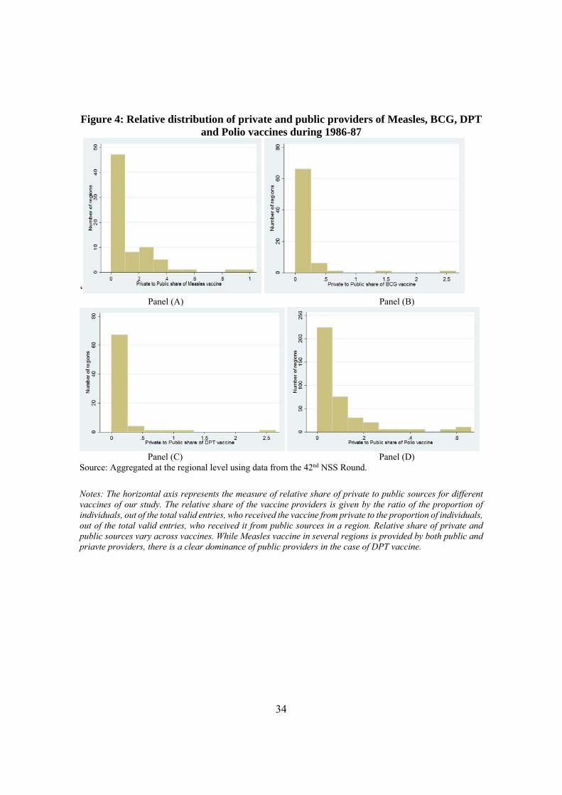
of variance vary across regions. Figure 4 panels A-D represent the distribution of regions

according to the share of private to public sources of demand for vaccination. We observe

regional variation for all vaccines but most regions to not have any representation of the

private sector in meeting the demand for vaccines. The dominant government role in the

provision of vaccines is almost completely flipped in the case of health care provision in

other areas such as pediatric care, prenatal and postnatal care. The ratio of private to public

demand is about 0.8, more than 5 times the ratio observed for vaccines. The statistics are

presented at various levels. In Section A, we present data from our baseline year (1986-87)

for each of the 76 regions. In Section B we present statistics on our outcomes (inequality) as

well as other control variables that vary over time. These statistics are therefore at the region-

year level. Finally, in Section C we present summary statistics from individual level data on

both disability and preferences that will be used in empirical tests of the validity of our

design.

Table 3 presents results from an OLS regression after pooling observations of the

years. The findings in column 1 of panel A suggests that a one standard deviation increase

in the private-public provision of vaccines results in a 1.5 percent increase in the Gini

coefficient. In column 2 we find that these results are robust to the inclusion of other control

variables at the state-region level (full list of control variables is provided in the footnote to

Table 3). In column 3, we also control for the private-public mix of hospitalisation in case

of child ailment. We find that the effect of the private-public mix in vaccine provision

continues to remain robust to this inclusion. Column 4 of panel A contain results when the

logarithm of variance is used as a measure of inequality. We find that a one standard

deviation increase in the private-public provision of vaccines results in about a 3 percent

increase in inequality, and the results remain robust when we control other variables (column

5) and non-vaccine health indicator (column 6).

We choose to focus on the private to public share of vaccine provision in this paper,

but panel B of Table 3 provides evidence that this focus is perhaps not too restrictive. In

panel B, we present the effect of private-public mix of non-vaccine sources of care on

inequality. We find that the effects of the non-vaccine variables is relatively small- ranging

from about one-eight (for effects on the Gini) and one-fifth (for effects on log variance) of

the effect observed for vaccines.

Although the coefficients for the Gini in panel A of Table 3 are robust to the inclusion

of other control variables, in the case where we use the logarithm of variance, the coefficients

21

decrease slightly as we move to a specification that includes control variables. This finding

suggests that the private-public mix of vaccines is not randomly distributed across state-

regions. We therefore also present results from an instrumental variable approach that uses

the private-public mix of the polio vaccine as an instrumental variable. The IV results in

Table 4 suggests that a higher private to public mix in vaccine provision results in higher

income inequality. As expected the standard errors of the point estimates of the IV

regressions are higher than that of OLS but the point estimates are higher and so the estimates

remain statistically significant. Further, the results are robust to the inclusion of other control

variables. Our IV regressions have high first-stage F statistics, above the required threshold

value of 10 (Staiger and Stock 1997). The IV results suggest that a one standard deviation

increase in private-public mix of measles increases the Gini coefficient by 2.2 percent and

the logarithm of variance by 4.3 percent. The estimates are similar for the case of DPT. For

BCGs, a one standard deviation increase in the private-public mix increases the Gini

coefficient by about 3 percent and the logarithm of variance by approximately 5.8 percent.

As noted previously due to the nature of selective investments in vaccines, our OLS

estimates are plausibly lower-bound estimates. Our OLS (Table 3) and IV estimates (Table

4) confirms this intuition with the IV point estimates being slightly larger than the OLS

estimates.

6.1 Robustness Check

6.1.1 Stability of coefficients over time

Our empirical strategy estimates the relationship between “baseline” measure of the relative

intensity of private to public demand for vaccines calculated using 1986-87 data and

subsequent inequality measures (1987-88 to 2011-12). Our regression results presented in

tables 3 and 4 include the pooled data over all the years. In Table 5, we test the sensitivity

of our estimates to including only specific years of data- starting from only including the

most recent year (2011-12) in column 1 and successively adding years in columns 2, 3 and

4. The OLS estimates for both the Gini and the logarithm of variance suggests a high degree

of robustness for the coefficient on the private-public mix of measles coverage. The

coefficient on the Gini is less robust when we only include the most recent data point, but

we note that this may be due to the very high standard error on the coefficient estimate- the

standard error in column 1 (0.035) is more than double the standard error in column 4

(0.017). Other than this exception, the coefficients on the Gini also remain robust to using

22

different years in analysis. The IV estimates for measles, DPT and BCG using the logarithm

of variance all suggest that our estimates are not very sensitive to the time period used in our

analysis. Once again, we note that the point estimates all remain relatively stable, but the

higher standard error (plausibly a result of the low sample size) when using the most recent

year renders the coefficient statistically insignificant. Indeed, to the extent that using more

current years data reduces the possibility of reverse causality, the findings bolster our

confidence that our estimates in Tables 3 and 4 may be interpreted as causal effects of the

private-public mix in the provision of vaccines on income inequality.

6.1.2 Stability of private-public mix of vaccine coverage

Our primary regressions use the baseline (1986-87) distribution of the private-public mix.

However, it is possible that the baseline distribution of the relative share itself changes over

time if Governments (or private providers) choose to make temporal changes in investments.

To assess this possibility, we first plot the ratio of private to public vaccine demand for BCG

vaccines in 1986-87 against the similar measure calculated in 1995-96. Figure 5 shows this

scatter. We find that there are two striking departures where the data point lies away from

the 45 degree line suggesting that, in these two regions, there is little stability in the private

to public demand for BCG vaccines.

We assess the sensitivity of our results when we drop the two outlier regions from our

analysis. When we control for the complete list of variables (similar to column 3 of Table

4), the point estimate on BCG is 0.083 (standard error = 0.033) in the case of the Gini and

5.050 (standard error = 1.743) in the case of the logarithm of variance.11  

6.1.3 Bias on the estimated coefficient on relative private share in the provision of

vaccines

We previously noted that direction of bias in the OLS estimates should be towards the null

since governments is more likely to invest in the poorer, high mortality areas and the private

sector is more likely to invest in the richer, low-mortality areas. However, it is possible that

individuals in regions where income inequality is higher also share preferences for health

systems in which public expenditure/investment is less relevant. In particular, it is possible

that individuals residing in high income inequality areas have lower preferences for publicly

11 Due to data constraints, we are unable to conduct sensitivity analysis for measles and DPT.

23

provided health care. In this case, there will be a positive correlation between the private-

public mix and income inequality, generating an upward bias in our OLS specifications. We

assess the strength of this hypothesis by examining whether regions of higher income

inequality also have lower preferences for government provided health care. The NSSO

survey data in 2004-05 has a specific question on whether the individual believes that the

government health care facilities are of poor quality. We create an indicator variable equal

to 1 if so, and 0 otherwise. We run a regression of this variable on income inequality. The

results are presented in Table 6 with the columns denoting estimates with and without

adjusting for other control variables. We find that inequality levels are not correlated with

preferences when we use the baseline inequality measure, regardless of the inequality

measure. When we use inequality measures as of 1993-94, we find insignificant coefficient

on the Gini, but find that higher variance in the logarithm of income (higher income

inequality) is associated with a greater preference for government public facilities. Overall,

our results suggest that we could continue to treat the OLS estimates as providing lower

bounds.

6.1.4 Threats to validity of the instrumental variable

The instrumental variable we use is the private-public mix of the polio vaccine. Although

we show (using our first stage F-statistic) that the IV is strongly correlated with the main

independent variable, it is possible that the IV is correlated with disability and hence

earnings and earnings inequality. The polio vaccine’s primary purpose is to prevent a

disability and disability is a known correlate of lower earnings. We therefore examine

whether our IV is correlated with disability. In 2002, the NSSO conducted a large national

survey to understand the prevalence and characteristics of disability in India. We use this

data and merge it with our instrumental variable-our baseline measure of private-public mix

of provision of the polio vaccine. The results are presented in Table 7 and suggest that there

is no correlation between the share of the private sector in the vaccine provision and

disability, a result that bolsters confidence in the validity of our IV.

7 Conclusion

In this paper we seek to establish both theoretically and empirically the link between the

relative shares of public and private health expenditures and cross sectional income

inequality. In a model where mortality is endogenous and is function of both public and

24

private health expenditures, we show that cross sectional income inequality is non-

decreasing in the share of private health expenditure.

We empirically test our theoretical prediction using region-level data from India.

Specifically, we examine the manner in which a higher share of the private sector in the

provision of vaccines affects income inequality. We use vaccination data on the relative

private-public share of vaccine provision in 76 regions in India in the year 1986-87. We also

use multiple household-level consumption expenditure survey rounds to construct inequality

measures within each region in India for the period spanning 1987-88 through 2011-12. OLS

regressions are potentially biased due to non-random investments in vaccines across regions.

Using the relative private-public share of the polio vaccine as an instrumental variable

approach, we examine the strength of the link between the relative private shares and income

inequality in an instrumental variable analysis. Our identification strategy rests on the

assumption that Government (or private) investments in the polio vaccine does not affect

mortality and hence inequality.

Estimates from both our OLS and IV models suggest that increasing the relative share

of private sources of health care provision is associated with an increase in expenditure

inequality. More specifically our OLS estimates for measles imply that a 1 standard

deviation increase in the relative private share in vaccine provision results in a 1.5 percent

increase in the Gini coefficient and a 3 percent increase in the variance of the logarithm of

income. Our findings based on the IV analysis suggest that a 1 standard deviation increase

in the relative private share results in a 2.2 % increase in the Gini and a 4.3 % increase in

the variance of the logarithm of earnings. As noted previously due to the nature of selective

investments in vaccines, our OLS estimates are plausibly lower-bound estimates and the

higher magnitude of the IV estimates confirms this intuition.

Although we focus on vaccines, we observe that the effects are also robust to the

inclusion of the private share in non-vaccine health care investments. Furthermore to the

extent that inequality is relatively permanent, we find that our results are also robust to the

inclusion of initial income inequality. Our primary results pool observations over the years

but in a robustness analysis we examine the sensitivity of our estimates to using cross-

sectional “snapshots” of our data and again find that the initial relative private share in

vaccines is related to subsequent income inequality.

Given the observational nature of the analysis, the findings are subject to a few

limitations. First, it is not possible to confirm the validity of our instrumental variable due

to data limitations. In particular, we cannot rule out the possibility that unmeasured factors

25

affect both income inequality and the instrumental variable. Nevertheless, we do posit that

the direction of the bias in our OLS estimates is most likely towards the null hypothesis

suggesting that our OLS estimates may be considered lower bound estimates. Second,

although we have used the demand for vaccines as a proxy for investments in health. It is

possible that at the regional-level, demand for vaccines is only an imperfect indicator for

actual investments. For example, although a particular region has heavy Government

investments in vaccines, the demand for Government sources may be low if households

perceive poor quality of the provider. Even so, to the extent that the relative private share in

demand measures the relative private share in health investment with random error, our OLS

estimates should once again be biased downward towards zero and hence provide a lower-

bound estimate of the true effect.

India has recently announced a new National Health Policy that seeks to rapidly increase

government investments in the health sector- a move that could increase the percent of

government health expenditure in overall GDP from 1.3 percent to 2.5 percent. Moreover, a

program titled Mission Indradhanush has been recently launched by the government and

seeks to ramp up the childhood vaccination rates to over 90 percent by the year 2020. If

these materialize in reductions in poor health outcomes, our findings suggest that the

increasing health investments envisaged by the Government of India could play a role in not

only improving health but in also lowering subsequent levels of income inequality.

References

[1] Basole, A., & Basu, D. (2015). Non-Food Expenditures and Consumption Inequality in

India. Economic and Political Weekly, 50(36).

[2] Becker, G. S. and N. Tomes (1979). An equilibrium theory of the distribution of income

and intergenerational mobility. Journal of Political Economy, 87 (6), 1153-1189.

[3] Bhattacharya, J., and Qiao, X. (2007). Public and private expenditures on health in a

growth model. Journal of Economic Dynamics and Control, 31(8), 2519-2535.

[4] Black, S. E. and P. J. Devereux (2011). Recent developments in intergenerational

mobility. Handbook of Labor Economics Volume 4, 1487-1541.

26

[5] Bloom, D. E., D. Canning, and J. Sevilla. 2004. “The Effect of Health on Economic

Growth: A production Function Approach." World Development 32 (1): 1-13.

[6] Castelló Climent, A., and Doménech, R. (2008). Human capital inequality, life

expectancy and economic growth. The Economic Journal, 118(528), 653-677.

[7] Chakraborty, S. (2004). Endogenous lifetime and economic growth. Journal of Economic

Theory, 116(1), 119-137.

[8] Chakraborty, S., & Das, M. (2005). Mortality, human capital and persistent inequality.

Journal of Economic Growth, 10(2), 159-192.

[9] Cowell, F.A. (2011). Measuring Inequality. Oxford University Press.

[10] Currie, J., & Hyson, R. (1999). Is the impact of health shocks cushioned by

socioeconomic status? The case of low birthweight (No. w6999). National bureau of

economic research.

[11] Deaton, A. (2003). Health, inequality, and economic development. Journal of Economic

Literature, 41(1), 113-158.

[12] Dottori, Davide. "Health funding, inequality and economic growth." Long-run Growth,

Social Institutions and Living Standards (2009): ed. Neri Salvadori and Arrigo Opocher.

[13] Figlio, D., Guryan, J., Karbownik, K., and Roth, J. (2014). The effects of poor neonatal

health on children’s cognitive development. American Economic Review, 104(12), 3921-

3955.

[14] Glomm, G., & Ravikumar, B. (1992). Public versus private investment in human

capital: endogenous growth and income inequality. Journal of political economy, 100(4),

818-834.

[15] Himanshu. (2007). Recent trends in poverty and inequality: some preliminary results.

Economic and Political Weekly, 497-508.

27

[16] Lahariya, C. (2014). A brief history of vaccines & vaccination in India. Indian Journal

of Medical Research, 139(4), 491.

[17] Mitra, A., and Mitra, S. (2016). Electoral Uncertainty, Income Inequality and the

Middle Class. Economic Journal (forthcoming).

[18] Pal, P. and Ghosh, J. (2007). Inequality in India: A survey of recent trends. DESA

Working Paper No. 45.

[19] Pickett, K. E., and Wilkinson, R. G. (2015). Income inequality and health: a causal

review. Social Science & Medicine, 128, 316-326.

[20] Stock J, Staiger D. (1997) Instrumental Variables Regression with Weak Instruments.

Econometrica. 1997;65 (3) :557-586.

[21] WHO, World Health Organization. 2001. “Macroeconomics and Health: Investing in

Health for Economic Development." Technical Report. Report of the Commission on

Macroeconomics and Health.

A. Appendix

In this section, we provide proofs of the propositions.

A.1 Proof of Proposition 1

For proof of this proposition, first observe that (15) implies that 0 for any , 0

for   and 0 for . Thus, the law of motion is convex for and then

linear thereafter. Also, it is continuous for all . To see this, is piece-wise continuous for and and, lim

→ lim →

.

*Existence: Graphically, the fixed points exist where the graph crosses the 45 degree

line. Since 0    0, the existence of the poverty trap fixed point is guaranteed.

Moreover, there may exist at most one more fixed point, 0 if and only if the long-run

growth rate along the sustained growth path satisfies

 > 1. To see this, suppose

1, then , for any . By 0 0 and the continuity of , its

graph crosses the 45 degree line for some . Conversely, suppose that the graph is

above the 45 degree line at but 1,then  too. This is contradictory. Suppose

28

even if exists, it is not along the convex part of the graph. So the fixed point is made at the linear part, where . This means that lim

→ ′ 1 1, but

lim→

′ g > 1, where

. Since   ∈   0,  1 , this is contradiction.12 This

implies that exists along the convex part as in Figure 2. Therefore, H crosses the 45

degree line just once for 0. Clearly, is stable and is unstable.

A.2 Proof of Proposition 2

From eq (15), 0. Since 0 (recall ≡ 1    ), the first result follows

immediately. Recall is the positive fixed point at which . Since an increase

in shifts up , it moves the fixed point to the left. From Proposition (1B) the long-run

growth rate is

. The result obtains because 0

B. Data Appendix on construction of additional variables used in analysis

B.1 Inequality

Gini coefficient, Logarithmic Variance and Variance of logarithms of consumer expenditure

data were computed at individual level using price-deflated measures of expenditure. We

referred to 42nd, 43rd and 50th NSS Survey Rounds to compute inequality for every state-

region.

1

1

∗

where is the mean of (income) and y∗ is the geometric mean of . We note that while

the logarithmic variance is a commonly used measure of inequality, the variance of

logarithms has also been used as an alternative (Cowell 2011). Since income data is

unavailable in the NSSO, we use per capita monthly consumption expenditure data to

compute our inequality measures.

12 The discussion indicates that there may exists infinite fixed points in a special case when 1. This case is rather non-generic and not interesting in terms of economic dynamics we aim to analyze. Also, this has a counter-factual economic implication that the sustained growth occurs only when the observed longevity reaches the biological limit. Thus, we do not consider it.

29

B.2 Per capita number of community health centers (CHC)

This serves as a proxy for the supply of public health care. It measures the number of

Community Health Centres reported during the Five year plan (1981-85), at the state level.

We use the state level population data from 1981 census to compute the per capita number

of CHCs in a state. This data is from Rural Health Statistics Report (2014-15)13, and the

population data is from the Planning Commission Report. For the newly formed states, such

as, Chhattisgarh, Jharkhand, Telengana or Uttarakhand, we use the same population numbers

as the corresponding original state (from which these new states were formed).

B.3 Non-Vaccine indicators

We used other proxy variables to understand the relative private to public mix in health care

delivery. For this we used the questions asked during 42nd NSS Round, whereby the

respondents had to indicate whether they received the care form private or public sources.

The questions asked were: (a) Whether the child was hospitalised on account of any

ailment/injury during the last 365 days, (b) Whether the mother was registered for prenatal

care in hospital or with doctor, (c) Whether the mother was registered for post-natal care in

hospital or PHC.

The common options stated for these questions were: NA; Public Hospital; Primary

Health Centre; Public Dispensary; Private Hospital; Nursing Home; Charitable institution

run by trust; government doctor; private doctor; Others. Any individual who received health

care from a public hospital or a primary health centre or a public dispensary or a government

doctor was categorized as having received health care form public sources. Everyone else

was categorized to have received it from private sources. This individual data was then

aggregated to regional level.

B.4 Disability due to Polio

This was derived at the individual level form the 58th Round (2002), Schedule 26 of the

Survey of Disabled Persons. The specific question was whether the individual reported any

disability; if so whether this was form birth and if not, then what is the cause of the disability.

Individuals who reported disability due to Polio were assigned a unit value and the others

assumed a value zero for this binary indicator variable.

13 Source: http://wcd.nic.in/sites/default/files/RHS_1.pdf 

30

Preference against Public health due to quality issue: This was computed at the

individual level from the 60th NSS Round (2004), Schedule 25. This question was asked to

individuals who reported any ailment during the last 15 days. The specific question was

whether any treatment was taken on medical advice; if yes, then whether any treatment

received from government sources. If the treatment was not sought from the government

sources, individuals were asked to list reasons for overlooking public facilities. The choices

were: (a) government doctor/facility too far; (b) not satisfied with medical treatment by

government doctor/facility; (c) Long waiting period before one can get appointment; (d)

required specific services not available; and (e) others. We generated a binary indicator

variable equal to 1 when individuals reported that they did not seek the government advice

as they were not satisfied with the quality. The others were assigned a zero value. The

variable proxies for strong preferences against using the public health facilities.

B.5 Imputed total Health Expenditure (% Gross State Domestic Product (GSDP))

Total health expenditure has public and private components. We obtain state level data on

Public health expenditure (as % Gross State Domestic Product) from the Health Care

Expenditure statistics from the Government of India for the period 1974-75 to 1990-99,

published by the National Institute of Public Finance and Policy.14  We use the public share

data as of 1986-87 (at current Prices). As private health expenditure data is unavailable, we

use an approximate ratio of Public to Private Hospitals, from Special Statistics on Health

Expenditure across States by Centre for Enquiry into Health and Allied Themes (CEHAT).

As the ratio is stated as 45.3 to 54.7, we use it to compute the private health expenditure (as

% Gross state Domestic Product). Finally, we add up the two components to derive the share

of total health expenditure (%GSDP).

14 See: http://www.nipfp.org.in/media/medialibrary/2014/10/HEALTH_CARE_EXPENDITURE_BY_GOVERNMENT_IN_INDIA_1947-75_TO_1990-91.pdf.  

31

Figure 1: Long-run effect of health care system on income inequality

Source: The World Bank Database; The Standardised World Income Inequality database (SWIID database) Notes: The horizontal axis represents the public health expenditure as percentage of total health expenditure as of 1995, which proxies the extent to which a country is leaning toward the public healthcare regime. The vertical axis is the Gini coefficient in 2010 based on disposable income. ISO 3166-1 alpha-3 nomenclature is used for the country codes.

32

Figure 2: Earnings dynamics under homogeneous households Fixed point equilibria

B. Earnings dynamics under different mix of private and public health expenditure

33

Figure 3: Dynamics of Gini coefficients under different private-public mix of health

expenditure

34

Figure 4: Relative distribution of private and public providers of Measles, BCG, DPT and Polio vaccines during 1986-87

‘ Panel (A) Panel (B)

Panel (C) Panel (D)

Source: Aggregated at the regional level using data from the 42nd NSS Round.

Notes: The horizontal axis represents the measure of relative share of private to public sources for different vaccines of our study. The relative share of the vaccine providers is given by the ratio of the proportion of individuals, out of the total valid entries, who received the vaccine from private to the proportion of individuals, out of the total valid entries, who received it from public sources in a region. Relative share of private and public sources vary across vaccines. While Measles vaccine in several regions is provided by both public and priavte providers, there is a clear dominance of public providers in the case of DPT vaccine.

35

Figure 5: Relative share of Private to public providers of BCG vaccine in 42nd and 52nd NSS Rounds

Notes: The horizontal axis depicts the relative share of private to public providers of BCG vaccines in 42nd NSS Round (1986-87). The vertical axis represents the same during the 52nd NSS Round (1995-96). Clustering of the points near the 45 degree line denotes that the regional pattern of the share of private to public provisioning did not change across the two survey rounds. From this, we can identify only two regions where the patterns differed over time. We treat them as potential outliers. These two regions are “Central Bihar” and “Himalayan West Bengal”.

36

Table 1: Baseline calibration

Parameter Description Calibrated value

Matching

Share of private expenditure in total health expenditure

0.7 Indian sample, 1995-2014

Effectiveness (scale) parameter of health expenditure

0.2866 Life expectancy, India 1985-2015

Elasticity of longevity increase with respect to health input

0.21 Life expectancy, India 1985-2015

Share of total (public + private) expenditure to consumption

0.05 Indian sample, 1995-2014

Effect of childhood health investment on human capital production

0.1 Dottori (2009). Also, Bloom, Canning, and Sevilla (2004) and WHO, World Health Organization (2001)

Scale parameter for human capital production

4.1548 Long-run annual growth of 2%

Sources: Indian data are obtained through World Bank Open Data.

37

Table 2: Summary statistics of variables used in analysis

Mean

Standard deviation

Measles 0.131 0.192 DPT 0.143 0.359 BCG 0.147 0.351 Polio 0.093 0.136

Where was child hospitalised for ailment 0.848 1.455 Where mother registered for prenatal care 0.812 1.204 Where mother registered for postnatal care 0.839 1.225 Per capita total CHCs Imputed total Health Expenditure (%GSDP)

0.017 4.021

0.029 3.511

Initial Inequality (Gini from 42nd NSS Survey)

0.814 0.022

Sample Size (N= 76) Section B Gini coefficient 0.533 0.071 Logarithm of variance 1.378 0.379 Variance of Logarithm 1.020 0.259 % population with secondary education 8.345 3.913 % Hindu population 77.953 23.769 % rural population 73.528 16.621 % scheduled caste (SC) 16.559 8.917 Sample Size (N= 379) Section C Disability due to Polio Sample Size (N= 78,827)

0.099

0.299

Preference against public health facilities due to poor perceived quality Sample Size (N= 29,516)

0.348 0.476

Notes: Section A - Each vaccine (measles, DPT, BCG and Polio) represents the relative share of private to public sources of vaccines in each region from the 42nd NSS round (1986-87). There are 76 observations corresponding to 76 regions.

38

Table 3: Pooled OLS estimates of the effect of relative private to public investments on

income inequality [Robust standard error]

Notes: Outcome variable is the Gini coefficient and the logarithm variance of per capita consumption expenditure at regional levels. Regressions are pooled ordinary least squares (OLS). Columns (1a) and (2a) are without any control variables. In columns (1b) and (2b) we control for the following control variables [m] rural population, education, social group, religion at the regional level, initial inequality from the 42nd round, per-capita number of community health centers (CHCs), and share of total health expenditure in the Gross State Domestic Product (GDSP), imputed with the average across states for the missing observations and year effects. Columns (1c) and (2c) control for a non-vaccine private-public health mix, in addition to the control variables used in Columns (1b) and (2b). The number of CHCs, the expenditure data and non-vaccine measures approximately correspond to our base year of analysis, 1986-87. Standard errors are corrected for heteroscedasticity and clustered at region level. *** significant at 1-percent level, ** significant at 5-percent level, * significant at 10-percent level.

Gini Coefficient Logarithm of Variance

Unadjusted for

control variables

Adjusted for control variables

[m]

Adjusted for control variables &a non-vaccine private-

public mix)

Unadjusted for control variables

Adjusted for

control variables

[m]

Adjusted for control variables & a non-

vaccine private-public mix

(1a) (1b) (1c) (2a) (2b) (2c) Panel A. Measles 0.041** 0.041** 0.035* 0.187* 0.175** 0.174** [0.021] [0.017] [0.018] [0.098] [0.079] [0.084] Place of child hospitalisation

0.004 [0.003]

0.003 [0.010]

Year effect Y Y Y Y Y Y R-squared 0.047 0.140 0.170 0.237 0.364 0.399 Sample Size 369 366 351 369 366 351 Panel B. Only using non-vaccine private to public mix: Place of child hospitalisation

0.005** [0.002]

0.005* [0.003] -

0.016 [0.01]

0.009 [0.009] -

Place of prenatal care

0.007*** [0.003]

0.006** [0.002]

- 0.035***

[0.012] 0.030*** [0.011]

-

Place of postnatal care

0.006** [0.003]

0.005* [0.003] -

0.033** [0.013]

0.014 [0.014]

-

39

Table 4: Instrumental variable estimates of the effect of relative private to public investments in vaccines on income inequality

[robust standard error]

Notes: Outcome variable is the Gini coefficient and the logarithm variance of per capita consumption expenditure at regional level. Columns (1a), (2a) and (3a) are without control variables. Control variables in columns (1b) and (2b) include the Share of rural population, Percentage of population with secondary education, social group and religion at the regional level. Columns (1c), (2c) and (3c) adjust for regional inequality measures from the 42nd Round, state level per capita CHCs and total health expenditure (% GSDP) at state level, in addition to the control variables used in Columns (1b) and (2b). Both the number of CHCs and the expenditure data approximately correspond to the base line year, 1986-87. The excluded instrumental variable in each case is the private to public ratio of the source of polio vaccine at regional level. First Stage F-statistic for Measles is 32.35; for DPT is 25.42; for BCG is 10.73. Standard errors are corrected for heteroscedasticity and clustered at region level. *** significant at 1-percent level, ** significant at 5-percent level, * significant at 10-percent level.

Gini Coefficient Logarithm of Variance Variance of logarithms

Unadjusted for control variables

Adjusted for control

variables

Adjusted for control variables, initial

inequality, per capita CHCs and total

health expenditure(%GSDP)

Unadjusted for control variables

Adjusted for

control variables

Adjusted for control variables, initial

inequality, per capita CHCs and total health expenditure(%GSDP)

Unadjusted for control variables

Adjusted for control variables, initial inequality, per capita CHCs and total health expenditure(%GSDP)

(1a) (1b) (1c) (2a) (2b) (2c) (3a) (3c) A. Measles 0.057** 0.055** 0.061** 0.324*** 0.281** 0.243** 0.258*** 0.202** [0.024] [0.022] [0.025] [0.122] [0.111] [0.119] [0.094] [0.088] B. DPT 0.052** 0.050** 0.053** 0.279** 0.250** 0.241* 0.224** 0.177** [0.023] [0.023] [0.023] [0.114] [0.113 ] [0.130] [0.089] [0.085] C. BCG 0.086** 0.083** 0.089** 0.504*** 0.439** 0.377** 0.400*** 0.314** [0.034] [0.033] [0.036] [0.177] [0.172] [0.184] [0.135] [0.135] Year effect Y Y Y Y Y Y Y Y

40

Table 5: Stability in regression coefficients over time [standard error]

2011-12 2009-10,

2011-12 2004-05, 2009-10, 2011-12

1993-94, 2004-05, 2009-10, 2011-12

(1) (2) (3) (4) Pooled OLS Log Variance

Measles 0.121 0.175** 0.152** 0.148** [0.127] [0.077] [0.069] [0.070] Sample Size 74 148 221 293 Variance of Logarithms

Measles 0.088 0.121** 0.111** 0.111** [0.079] [0.052] [0.047] [0.048] Sample Size 74 148 221 293

Gini

Measles -0.004 0.031 0.035* 0.035** [0.035] [0.021] [0.019] [0.017] Sample Size

74

148

221

293

Instrumental variable analysis Logarithmic Variance Measles

0.203

0.292**

0.260**

0.245**

[0.188] [0.130] [0.117] [0.111] DPT

0.190

[0.177]

0.255** [0.119]

0.225** [0.110]

0.221* [0.112]

BCG 0.301 0.415** 0.368* 0.345* [0.276] [0.206] [0.188] [0.187]

Notes: The unit of observation is region-year. Outcome variable is the Gini coefficient and the logarithm variance of per capita consumption expenditure at regional level. The five survey rounds considered for analysis are- 43rd round (1987-1988) 50th round, (1993-1994); 61st round, (2004-2005); 66th round, (2009-2010) and 68th round, (2011-2012). Column (1) uses the latest Consumer Expenditure NSS Survey (68th) and the relative private to public vaccine sources from the 42nd NSS Round; Column (2) uses the latest two Consumer Expenditure NSS Surveys (68th & 66th); Column (3) uses the latest three Consumer Expenditure NSS Surveys (68th, 66th and 61st); Column (4) uses the latest four Consumer Expenditure NSS Surveys (68th, 66th, 61st and 50th). The control variables used in all the columns include the Share of rural population, Percentage of population with secondary education, social group, religion and year effects. The excluded instrumental variable is the private to public ratio of the source of polio vaccine at regional level. Standard errors are corrected for heteroscedasticity and clustered at region level. *** significant at 1-percent level, ** significant at 5-percent level, * significant at 10-percent level.

41

Table 6: Relationship between preferences for public health facilities and income inequality [robust standard error]

Preference against using public health facility as the service quality is not satisfactory (2004)

Unadjusted Adjusted for control variables

(1) (2) Inequality in 1987-88 (43rd Round) Gini -0.195 -0.134 [0.332] [0.334] Logarithm of variance -0.008 -0.014 [0.056] [0.057] Sample size 29,513 29,341 Inequality in 1993-94 (50th Round) Gini -0.221 -0.143 [0.406] [0.398] Logarithm of variance 0.005 0.002 [0.074] [0.075] Sample size 29,323 29,151

Notes: This table reports Pooled OLS results. Dependent variable is a binary variable equal to 1 if individuals preferred not to use the government sources for treatment because they were not satisfied with the quality. All other individuals who opted for public or private sources of treatment for other reasons assumed an indicator value, zero. Data on preference comes from the 60th NSSO Survey on Morbidity & Health care (2004). The inequality measure is at regional level from the 43rd NSS Survey (1987-88). We also separately use inequality measures from the 50th NSS Survey (1993-94). Control variables include age, sector and social group of the individuals. Standard errors are corrected for heteroscedasticity and clustered at region level. *** significant at 1-percent level, ** significant at 5-percent level, * significant at 10-percent level.

42

Table 7: Relationship between ratio of private-public investments in polio vaccine on subsequent disability due to Polio [robust standard error]

Cause of disability due to Polio (2002)

Polio as the cause of disability (unadjusted)

Polio as the cause of disability (adjusted)

(1) (2) Private-public polio vaccine in 1986-87 -0.023 -0.022

[0.025] [0.024]

Sample size 78,827 78,709

Notes: This table reports Pooled OLS results. Dependent variable is a binary variable equal to 1 if an individual reports disability due to Polio. All other individuals, reporting disability due to other reasons assume a value zero. Data on disability comes from the 58th NSSO Survey of Disabled Persons (2002). Private-public sources of the polio vaccine is at region level, from the 42nd NSS Round. Column (1) is without any control variable. Column (2) controls for sector, Class according to expenditure level, social group, general education of the principal earner in the household. Standard errors are corrected for heteroscedasticity and clustered at the region level. *** significant at 1-percent level, ** significant at 5-percent level, * significant at 10-percent level.