HD Maps: Fine-grained Road Segmentation by Parsing Ground and AerialImages

Gellert MattyusRemote Sensing Technology Institute

German Aerospace Centergellert.mattyus@dlr.de

Shenlong Wang, Sanja Fidler, Raquel UrtasunDepartment of Computer Science

University of Torontoslwang, fidler, urtasun@cs.toronto.edu

Abstract

In this paper we present an approach to enhance exist-ing maps with fine grained segmentation categories such asparking spots and sidewalk, as well as the number and lo-cation of road lanes. Towards this goal, we propose an ef-ficient approach that is able to estimate these fine grainedcategories by doing joint inference over both, monocularaerial imagery, as well as ground images taken from astereo camera pair mounted on top of a car. Important tothis is reasoning about the alignment between the two typesof imagery, as even when the measurements are taken withsophisticated GPS+IMU systems, this alignment is not suf-ficiently accurate. We demonstrate the effectiveness of ourapproach on a new dataset which enhances KITTI [8] withaerial images taken with a camera mounted on an airplaneand flying around the city of Karlsruhe, Germany.

1. IntroductionWe are in an exciting time for computer vision, and more

broadly AI, as the development of fully autonomous sys-tems such as self-driving cars seems possible in the nearfuture. These systems have to robustly estimate the scenein 3D, its semantics as well as be able to self-localize at alltimes. Key to the success of these tasks is the use of mapscontaining detailed information such as road location, num-ber of lanes, speed limit, traffic signs, parking spots, trafficrules at intersections, etc.

Current maps, however, have been created with the useof semi-automatic systems that employ many man-hours oflaborious and tedious labeling. An alternative to this costlylabeling is to employ existing maps and correct/enhancethem based on ground imagery or LIDAR point clouds, cap-tured, for example, by a Velodyne/cameras mounted on topof a car. Systems like TESLA auto-pilot [1] are currentlyusing their deployed fleet of cars, which are equipped withcameras, to perform such corrections. However, it is dif-ficult to create full coverage of the world as we will need

access to imagery/LIDAR from millions of cars in order toreliably enhance maps at a world-scale.

Alternatively, aerial images provide us with full coverageof a significant portion of the world, but at a much lowerresolution than ground images. This makes semantic seg-mentation from aerial images a very difficult task. In thispaper, we propose to use both aerial and ground images tojointly infer fine grained segmentation of roads. Towardsthis goal, we take advantage of the OpenStreetMap (OSM)project, which provides us with freely available maps of theroad topology in the form of piece-wise linear road seg-ments. We formulate the problem as energy minimization,inferring the number and location of the lanes for each roadsegment, parking spots, sidewalks and background, as wellas the alignment between the ground and aerial images. Weemploy deep learning to estimate semantics from both aerialand ground images, and define a set of potentials exploitingthese semantic cues, as well as road constraints, relation-ships between parallel roads, and the smoothness of boththe estimations along the road as well as the alignment be-tween consecutive ground frames.

We demonstrate the effectiveness of our approach in anew dataset which covers a wide area of the city of Karl-sruhe in Germany, both from the ground and from the air.We provide pixel-level annotations for the aerial images interms of fine-grained road categories. We call our datasetAir-Ground-KITTI. We show that our approach is able toestimate these categories reliably, while significantly reduc-ing the alignment error between the ground and aerial im-ages when compared to a sophisticated GPS+IMU system.

2. Related work

For several decades, researchers from various communi-ties (e.g., vision, remote sensing) have been working on au-tomatic extraction of semantic information from aerial im-ages. In the following, we summarize the approaches mostrelevant to our work.

1

Figure 1. Illustration of our model: (a) Parameterization of our approach. Our random variables are the absolute location of the differentregion boundaries (e.g., sidewalk) as well as the alignment between air and ground. (b) Our formulation allows a random variable to takethe same state as the previous node, collapsing a region to have 0 width. (c). For each ground-view image, a random variable models thealignment noise. (d). Projection of our parameterization on the ground-view.

Aerial image parsing: Early approaches employed prob-abilistic models that aimed to produce topologically con-nected roads. [2] defined a probabilistic model that tiled theimage into patches, performed road inference inside eachpatch via dynamic programming, and then “stitched” to-gether high-confidence patches to ensure road connectiv-ity. Recent work exploits learned classifiers to perform se-mantic segmentation. [15, 16] trained a neural net to clas-sify pixels in local patches as road. They employ a post-processing step to ensure a consistent road topology acrossthe patches, which is, however, prone to block-effects. [26]segments the road by defining an MRF on superpixels.High-order cliques are sampled over straight segments orjunctions to encourage a road-like network structure. Due tocomplexity of high order terms a sampling scheme is usedto concentrate on more important cliques. [4] samples graphjunction-points using image consistency and shape priors.A full review of this large field is out of scope of this paper,and we refer the reader to [14] for a detailed review.

Aerial parsing with maps: While proven useful in manycomputer vision and robotics applications [9, 13, 3, 25],few works employ map information for parsing aerial im-ages. [20] uses a screenshot of the vector map as a weaksource of ground-truth for training a road classifier. [27]exploit road center-lines from OSM maps as a ground-truthroad location and performs road segmentation by estimat-ing the width of the road. This is done by finding bound-aries of superpixels along the direction of the road, and ig-noring dependencies across different line (road) segments.However, the alignment between OSM and aerial imagesis far from perfect. To solve this problem, [12] proposed aMRF which reasons about re-positioning the road centerlineand estimating the width of the road. Smoothness is incor-porated between consecutive line segments by encouragingtheir widths to be similar. In our work we go beyond thisapproach by introducing a formulation that reasons about

more fine-grained road semantics such as lanes, sidewalksand parking spots, and exploits simultaneously aerial im-ages as well as ground imagery to infer this information.

Fine-grained road parsing: Very few works exist thatextract detailed segmentation. [17] propose a hierarchicalprobabilistic grammar to parse smaller-scale aerial regionsinto roads, buildings, vehicles and parking lots. Classifiersare first employed to generate object/building/vegetationproposals while the grammar imposes semantic and geo-metric constraints in order to derive the final parse. Learn-ing and inference are both hard in grammars, and computa-tionally expensive sampling techniques typically need to beemployed. In our work, we are aiming at a detailed pars-ing of the roads into sub-categories. Unlike [17], we exploitOSM information in order to derive an efficient formulation.

The work most related to ours is [21] which exploits themap as a screenshot of the road vector map to perform roadand lane estimation. The authors take a pipeline approach,where, in the first step, road lane hypotheses are generatedbased on the output of the road classifier and detected lanemarkings. In the second step, the authors provide heuris-tics to “track” the lane hypotheses and connect them into asingle lane labeling.

Aerial-to-ground reasoning: Recent work aims to ex-ploit both aerial and the ground-view, mainly for the prob-lem of geo-localization. In [11], a deep neural network isused to match ground images with aerial images in obliqueviews. The matches come from facade to facade matchingand therefore can not be extended to orthographic aerial im-ages. In [22], 3D reconstructions from the ground imagesare matched to oblique views of aerial images. [10] learncross-view matching between ground images, aerial ortho-graphic photos and land cover attributes. This extends theimage geolocalization to areas not covered by ground im-ages. Forster et al. [7] match the computed 3D maps of

(a) Along Road (b) Perpendicular to Road (c) Along ground image sequence

Figure 2. BCD: The graph shows a simplified network with two parallel roads (each with 3 random variables) and one ground imageper segment connected to the right road. BCD alternates between three types of updates. (a) Along the road updates: we optimize overeach chain with the same color (while holding all other variables fix). The pairwise terms fold to unaries (see dashed black lines). (b)Perpendicular to the road updates: we do inference for the nodes with the same color (holding the rest fix). (c) Along the ground alignments:We minimize only the t variables which are depicted in green. The y variables are fixed and are depicted in black.

MAVs and ground robots for localization and map augmen-tation. This method relies on matching 3D information andtherefore needs multiview images both from above and onground. In our work, we exploit the maps as well as groundand aerial imagery to perform fine-grained road parsing. Weare not aware of prior work that tackles this problem.

3. Fine-grained Semantic Parsing of RoadsWe now describe our model that infers fine-grained se-

mantic categories of roads from aerial and ground images.In particular, we are interested in estimating sidewalks,parking, road lanes as well as background (e.g., vegetation,buildings). Towards this goal we exploit freely availablecartographic maps (we use OSM), that provide us with thetopology of the road network in the area of interest. Ourapproach takes as input an aerial image xA, a road map xM

and a set of ground stereo images xG, which are taken by acalibrated stereo pair mounted on top of a car. The map xM

is composed of a set of roads, where each road is defined asa piece-wise linear curve representing its centerline.

3.1. Model Formulation

We formulate the problem as the one of inference in aMarkov random field (MRF), which exploits deep featuresencoding appearance in both aerial and ground images,edge information, smoothness in the direction of the road aswell as restrictions between parallel roads to avoid doublecounting the evidence. Our model encodes each street seg-ment in the aerial image with 15 random variables encodingall possible combinations of background (B), sidewalk (S),road lanes (L) and parking (P). In particular,

y = (y1, · · · , y15)

= (B1, S1, B2, S2, P1, L, P2, S3, B3, S4, B4)

with B1, B4 the rightmost (leftmost) border of the back-ground. We model roads with up to 6 lanes, i.e., L =(L1, L2, L3, L4, L5, L6). We allow all variables (but L6)to take the state of the previous random variable in the se-quence (i.e., yi = yi−1), encoding the fact that some of

these regions might be absent, e.g., there is no parking orsidewalk. This is not the case for L6 forcing the fact thatat least one lane should be present. We define the states ofeach random variable to be [−15, 15]m from the projectionof the OSM centerline in the aerial image (Fig. 1). Thisdiscretization represents pixel increments. Note that whilethere are 15 random variables, y defines 16 different re-gions as B1 and B4 are not limited on the left (right). Eachregion width is simply defined by wi = yi − yi−1, whilethe width of B1 is defined as w1 = −15m + y1, and thewidth of B4 as w16 = 15m − y16, since −15m and 15mare the beginning and end of the state space. Note that thecombination (B,S,B, S) is necessary (both on the left andright), as there are many bike lines in Germany (where ourimagery is captured), and it is not possible to distinguishthem from the sidewalk. Fig. 1 illustrates the model.

Each of our ground images comes with a rough align-ment with the aerial image as we have access to aGPS+IMU and the cameras are registered w.r.t these sen-sors. This alignment is, however, noisy with 1.67m erroron average. Thus, our model reasons about the alignmentwhen scoring the ground images. Towards this goal, we de-fine t = (t1, · · · , tn) to be a set of random variables (oneper ground image) representing the displacement in the di-rection perpendicular to the OSM road segment. We definethe state space of each misalignment to be ti ∈ (−4m, 4m).This is discretized to represent pixel increments.

We define the energy of the MRF as to encode the infor-mation contained in the ground and aerial images as well assmoothness terms and constraints on the possible solutions:

E(y, t,xA,xM ,xG) = Eair(y,xA) + Eground(y, t,xG)

+ Esmooth(y, t,xM ) + Econst(y)(1)

We now define the potentials we employ in more detail.

Aerial semantics: We take advantage of deep learning inorder to estimate semantic information from aerial images.In particular, we create pixel-wise estimates of 5 semanticcategories: road, sidewalk, background, building and park-ing. We exploit the CNN for segmentation [23, 19] trained

GPS+IMU Our alignmentFigure 3. Effect of reasoning about alignment: (left) alignmentgiven by GPS+IMU, (right) alignment inferred by our model.(top) Ground road classifier projected into the aerial image (shownin red). (bottom) Our semantic classes projected on the groundimage. Our joint reasoning significantly improves alignment.

on ILSVRC-2014, which we fine-tune for a 5-label clas-sification task: road, parking spot, sidewalk, building andbackground. To train the network we created training exam-ples by extracting patches centered on the projection of theOSM road segments. If the road segment is too long (i.e.,long straight road) we create an example every 20m. Wefurther perform data augmentation by applying small rota-tions, shifts and flips to the training examples. The output ofthe soft-max is a downsampled segmentation. To create ourfeatures, we upsample the softmax output using linear inter-polation as in [5]. To save computation, we only apply thenetwork in the region of interest (regions of the image thatare close to OSM roads). The aerial semantic potential thenencodes the fact that our final segmentation should agreewith the semantics estimated by the deep net. Towards thisgoal, we define 5 features for each of our 16 regions, oneper label of the deep net. Each feature simply aggregatesthe output of the softmax in that region. Recall that eachregion is defined by two consecutive random variables, e.g.the first sidewalk is defined by y1, y2, that is B1, S1. Werefer the reader to Fig. 1 for an illustration. While this po-tential seems pairwise in nature, we can further decomposeit into unary potentials via accumulatorsA perpendicular tothe road direction. These are simply generalizations of inte-gral images from axis aligned accumulators to accumulatorsover arbitrary directions. We thus define

φcl(yji , y

ji−1) =

∑p∈Ωj

i (yji ,y

ji+1)

ϕ(p) = A(yji+1)−A(yji )

with yji the i-th variable of the j-th road segment, and ϕ(p)the softmax output interpolated at pixel p. To compute thisfeatures, we only need 5 accumulators per road segment,one for each semantic class that the deep net predicts.

Aerial edges: This potential encodes the fact that the lo-cation of the boundaries between regions should be close

0 0.1 0.2 0.3 0.4 0.5 0.6 0.7

precision

0.2

0.3

0.4

0.5

0.6

0.7

0.8

0.9

reca

ll

Precision-Recall Curves

road

road*

sidewalk

parking

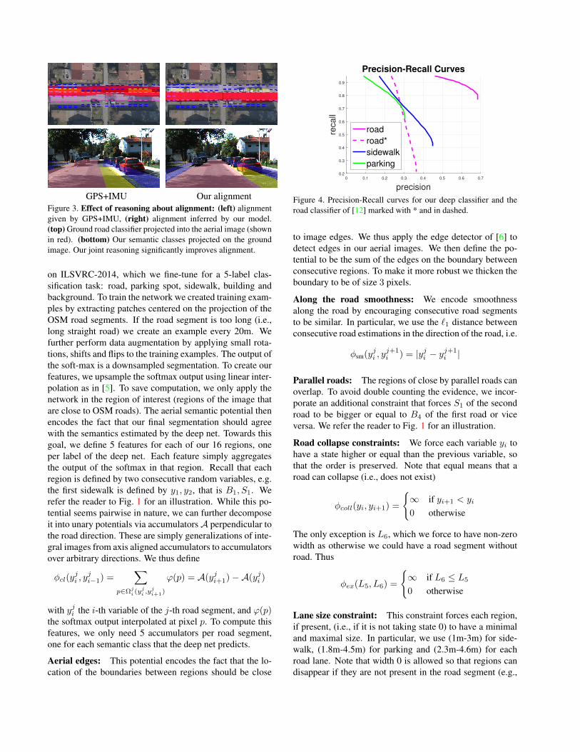
Figure 4. Precision-Recall curves for our deep classifier and theroad classifier of [12] marked with * and in dashed.

to image edges. We thus apply the edge detector of [6] todetect edges in our aerial images. We then define the po-tential to be the sum of the edges on the boundary betweenconsecutive regions. To make it more robust we thicken theboundary to be of size 3 pixels.

Along the road smoothness: We encode smoothnessalong the road by encouraging consecutive road segmentsto be similar. In particular, we use the `1 distance betweenconsecutive road estimations in the direction of the road, i.e.

φsm(yji , y

j+1i ) = |yji − y

j+1i |

Parallel roads: The regions of close by parallel roads canoverlap. To avoid double counting the evidence, we incor-porate an additional constraint that forces S1 of the secondroad to be bigger or equal to B4 of the first road or viceversa. We refer the reader to Fig. 1 for an illustration.

Road collapse constraints: We force each variable yi tohave a state higher or equal than the previous variable, sothat the order is preserved. Note that equal means that aroad can collapse (i.e., does not exist)

φcoll(yi, yi+1) =

∞ if yi+1 < yi

0 otherwise

The only exception is L6, which we force to have non-zerowidth as otherwise we could have a road segment withoutroad. Thus

φex(L5, L6) =

∞ if L6 ≤ L5

0 otherwise

Lane size constraint: This constraint forces each region,if present, (i.e., if it is not taking state 0) to have a minimaland maximal size. In particular, we use (1m-3m) for side-walk, (1.8m-4.5m) for parking and (2.3m-4.6m) for eachroad lane. Note that width 0 is allowed so that regions candisappear if they are not present in the road segment (e.g.,

(a) Intersection with tram line. (b) Small town.

(c) A road with three lanes. (d) Two roads with tram stop in between.

(e) Dense urban area. (f) Splitting road plus a bike lane along the street.Figure 5. Visualization of our semantic road parsing results using only aerial images. The road lanes are shown with shades of pink, thesidewalk with blue and the parking spots with yellow.

we only have two lanes, there is no sidewalk on the high-way). The intervals for the lanes are estimated based on thestandards of German roads, while the sidewalk and parkingintervals are computed based on empirical estimates.

Centerline prior: As our images are well registered withOSM, we include a prior that the centerline of our modelshould be close to the centerline of OSM. In particular,

φcen(L3) =

||L3 − l||2 if − 7.5 ≤ L3 ≤ 7.5

∞ otherwise

with l the location of the centerline.

Ground semantics: We take advantage of deep learningin order to estimate semantic information from ground im-

ages. We exploit the VGG [23] implementation of [19]trained on PASCAL VOC, which we fine-tuned to predictthe same 5 classes as the aerial semantics (road, park-ing, sidewalk, building and background). We estimate theground plane from the stereo image and project pixels be-longing to this plane to the aerial image via a homography.We then define our ground semantic potential to encouragethe segmentation to agree with the aligned ground imagesegmentation projected to the aerial image. Towards thisgoal, we define 5 features for each of our road regions, eachcounting the amount of softmax output for the given class:

φground(tk, yji , y

ji−1) = G(tk, y

ji+1)− G(tk, y

ji )

Note that via the integral accumulator the 3-way potentialdecomposes into pairwise terms G(t, y). In this case we

Aerial GroundFigure 6. Left: The ground road detection with red projected into the aerial image after alignment and road layout estimation. Right:The semantic lanes projected back into the aligned ground image. These scenes are all challenging with parallel roads, parking spots andintersections. The bottom image is especially difficult since it is an urban pedestrian area. Note that the aerial and ground images weretaken with several years difference in different seasons. Pink is road, blue is sidewalk and yellow marks parking spots.

only need 5 integral accumulators per ground image.

Ground alignment smoothness: This potential encodesthe fact that two consecutive alignments should be similar.

φgsm(tk, tk+1) = |tk − tk+1|

This assumes that GPS+IMU have smooth errors and nooutliers.

3.2. Inference via Block Coordinate Descent (BCD)

Inference in our model can be performed by minimizingthe energy function:

y∗, t∗ = argminy,t

E(y, t,xA,xM ,xG)

with E(y, t,xA,xM ,xG) defined as in Eq. (1). Unfortu-nately, inference in our model is NP-hard, as our graphi-cal model contains many loops. We thus take advantage ofblock coordinate descent to perform efficient inference. Werefer the reader to Alg. 1 and Fig. 2 for inference steps.

Our block coordinate descent algorithm (BCD) alter-nates by doing inference in the direction along the road,

doing inference in the direction perpendicular to the roadand aligning the ground and aerial images. Note that whena road is not connected to a parallel road, the second stepresults in a graphical model with 15 variables, while whenthere are k parallel roads, this involves doing inference overa graphical model with 15k variables. Note also that in or-der to minimize the same objective, each of these iterationsis performing conditional inference, and the pairwise po-tentials involving variables that are not optimized collapseto unaries.

3.3. Training with S-SVM

We employ structured SVM (S-SVM) [24] to learn theweights of the aerial unaries and the smoothness in ourmodel. In particular, we use the parallel cutting plane im-plementation of [18]. We employ a combination of twoloss functions. The first is a truncated L2 loss: `data =min(||yji − y

ji ||2, 100m2), encouraging our prediction yji to

be close to the ground truth yji . We compute yji by perform-ing inference in our model with features computed from theground truth annotation (segmentation). The second lossterm encourages smoothness of the prediction along the

Algorithm 1 Block coordinate descent inference (BCD).1: Set all alignments t = 0, and initialize y by minimizing

Eq. (1) ignoring the along road smoothness.2: repeat3: for for all yj do4: Minimize Eq. (1) along the road w.r.t yj , holding

the rest fixed.5: end for6: for all yi at one segment of the road do7: Minimize Eq. (1) w.r.t yi, holding the rest fixed.8: end for9: for all t variables do

10: Minimize Eq. (1) w.r.t t, holding y fixed.11: end for12: until no energy reduction or max number iterations

road, `sm = |yji − yj+1i |. Note that the geometrical con-

straints in our model are either 0 or∞ and are not trained.

4. ExperimentsWe collected a new dataset which we call Air-Ground-

KITTI, which is composed of both ground images fromthe KITTI tracking benchmark [8] and newly acquired or-thorectified aerial images over the same area. We neglectedthe KITTI sequences where the car is mostly static, result-ing in 20 KITTI sequences for a total of 7603 ground stereoimages. We annotated every 30th ground image with 4semantic classes (parking, sidewalk, road, building). Theaerial images were acquired by a DSLR camera mountedon an airplane and projected on the earth surface with 9cm/pixel Ground Sampling Distance (GSD). We split thedata into 10 training and 10 test aerial image/KITTI se-quences, with special care to avoid overlaps in the aerial im-ages. We manually annotated the aerial images with 4 cat-egories (parking, sidewalk, road, building) as closed poly-gons and the lane markings as polylines. This took 70h ofannotation, at a mean of 21h/km2, the area is 3.23 km2.

To perform fine-grained segmentation using both aerialand ground images, we estimate a homography that trans-forms the ground plane in KITTI to the UTM coordinatesystem based on the KITTI’s GPS+IMU measurements andthe camera calibration. We assign each ground image tothe closest parallel road segment. Our model then refinesthis estimate in the direction perpendicular to each road seg-ment. We process every 5th ground image in the sequence.

As metrics for the fine-grained segmentation we calcu-late the pixelwise Intersection over Union (IoU), Precision,Recall and F1 metrics for three classes (i.e. road, parking,sidewalk). Note that we only measure the areas laying inthe area of interest (i.e. ±15m around the road map center-line). We consider two parallel roads overlapping over thesame area as a serious error. To reflect this, we handle these

(a) (b)

(c) (d)

(e) (f)Figure 7. It is hard to estimate the number of lanes if there areno lane markings. (a) Our method, (b) Oracle (i.e., our methodwith ground truth potentials). (c) The OnlyLane model without theparallel constraint allows the road to ”jump” to the nearby parallelroad. (d) The parallel constraints of LaneRoadParallel preventsthis from happing. (e) Dense, urban pedestrian streets are difficultto estimate. (f) Our model is not intended for intersections, as itdoes not reason about turn lanes.

areas as if they were background. The metrics in Table 1are calculated according to this.

For the roads, we additionally compute whether we haveestimated the correct number of lanes. This is measured asthe average `1 error in terms of number of lanes (EN). Notethat if there are no lane markings, estimating the number oflanes is very difficult. Fig. 7 (a-b) shows this difficulty.

In our experiments, we compare our approach to thestate-of-the-art method of [12], which uses OSMs to es-timate road width. We also tested different model con-figurations for our approach. We refer to Lane as amodel that employs Aerial semantics, Aerial Edges, Roadcollapse constraints, Lane size constraint and Centerlineprior energy terms. Inference is done independently foreach road segment via dynamic programming along theyj = yj1, · · · , y

j15 chains. We refer by LaneParallel to a

model where we additionally include the constraint betweennearby parallel road. We refer by LaneRoad as a model thatcontains all the potentials in Lane plus smoothness along theroad. We apply BCD inference by alternating between thechains perpendicular to the road (the lanes) and along theroads (segments). We refer by LaneRoadParallel a modelthat contains all potentials but the ground. Finally, Groundcontains all potentials. We evaluate this case only whereground images are available.

ModelAverage Road Sidewalk Parking

IoU F1 IoU F1 Pr. R. EN IoU F1 Pr. R. IoU F1 Pr. R.Mattyus et al. [12] - - 62.1 76.4 68.0 87.0 - - - - - - - - -

[12] Deep Un* - - 64.4 78.4 66.7 94.7 - - - - - - - - -Lane 43.6 59.6 61.9 76.5 82.8 71.0 0.730 31.8 48.3 67.2 37.7 37.0 54.1 58.5 50.3

LaneParallel 44.8 60.3 66.5 79.9 85.0 75.4 0.543 31.6 48.0 69.8 36.6 36.1 53.1 70.8 42.4LaneRoad 45.4 61.6 61.9 76.4 82.7 71.0 0.707 38.3 55.4 62.4 49.7 36.1 53.1 52.2 54.1

LaneRoadParallel 48.6 64.3 68.0 80.9 83.5 78.5 0.555 39.5 56.6 63.5 51.1 38.4 55.5 63.8 49.1LaneRoadParallel** 41.9 58.5 54.9 70.9 86.9 59.9 0.559 34.9 51.7 68.7 41.5 35.8 52.7 69.9 42.3

Full** 42.0 58.6 55.3 71.2 86.8 60.4 0.556 34.9 51.7 68.7 41.5 35.8 52.7 69.9 42.3

Table 1. Performance for the semantic classes (i.e. road, parking spot, sidewalk) with various models and the two baselines. The values arein %, except EN which is the average road lane number l1 error with respect to the oracle. * Marks the method of [12] with our deep roadclassifier. The last two rows marked with ** evaluate only over areas where ground images are also available.

GPS+IMU [m] Ours [m]Alignment error 1.67 0.57

Table 2. Ground to air image misalignment based on the cameracalibrations (GPS+IMU) and after our alignment measured in me-ters. Using ±4 meter interval.

Comparison to the state-of-the-art: As shown in Ta-ble 1, our method outperforms [12] in almost all metrics,even when we apply our deep features instead of their roadclassifier in their method. Furthermore, we retrieve moresemantic categories such as sidewalk, individual road lanesand parking. The constraint between parallel roads is im-portant to achieve good results on roads. Without it, ourmodel cannot outperform [12], which has this constraint.

Deep semantic features in aerial Images: We show theperformance of our Deep Network in Fig. 4. Note that it ismuch better than the road classifier of [12].

Alignment between aerial and ground images: Asshown in Table 2 and Fig. 3 reasoning about the alignmentbetween ground and aerial images while doing fine-grainedsegmentation improves the alignment significantly.

Qualitative Results: We visualize our results when usingonly aerial images in Fig. 5, and when using joint aerialand ground reasoning in Fig. 6. Our approach is able toestimate well the lanes, sidewalk and parking as well as thealignment between the ground and the aerial images.

Ablation studies: As shown in Table 1, the metrics fordifferent versions of our model are fairly similar, howeverqualitatively, as we add more potentials, the results get bet-ter. This is illustrated in Fig. 7 (c), where the OnlyLanemodel moves the middle road to a parallel road resulting ina noncontinuous structure. In contrast, the LaneRoadParal-lel model prevents overlaps and favors smoothness, see theFig. 7 (d). Including the ground images only slightly im-proves performance. We believe this could be overcome byusing stronger features in the ground images, i.e., leverag-ing the full 3D point cloud, not just the ground plane. Note

that since our approach gives us very precise alignments be-tween the ground and the aerial images it could be used toenhance OSM with object locations, e.g. traffic signs.

Inference time: Inference in our full model takes 6 sec-onds per km of road, with a single thread on a laptop com-puter. Note that BCD can easily be parallelized.

Limitations: Our model is designed for individual roadsand it does not reason about turning lanes connecting dif-ferent roads at intersections (see Fig. 7 (f)). Dealing withsuch scenarios is part of our future work. Semantic seg-mentation from aerial images reasons mainly about the vis-ible parts of the street. Therefore covered areas (e.g. bybuilding, bridges, trees) can be a problem. However, whenground images are available, our approach can handle thisproblem. Our aerial images were acquired in early spring,and thus trees occluding the roads is not a big problem.

5. ConclusionWe proposed an approach to enhance existing freely

available maps with fine grained segmentation categoriessuch as parking spots and sidewalk, as well as the numberand location of road lanes. Towards this goal, we proposedan efficient method that produces very accurate estimatesby performing joint inference over both, monocular aerialimagery captured by a plane and ground images taken froma stereo pair mounted on top of a car. We have demon-strated the effectiveness of our approach on a new datasetwhich enhances KITTI with aerial images taken with a cam-era mounted on an airplane and flying around the city ofKarlsruhe. In the future, we plan to reason about other finegrained categories such as traffic signs in order to furtherenhance the maps. As our method reasons about the accu-rate alignment between the map and the ground images, weenvision its use for precise, lane-wise self localization of thevehicle on the road.

AcknowledgmentsWe would like to thank Viktoria Zekoll, Stefan Turzer and

Mark Bagdy for making the laborious annotation work.

References[1] http://fortune.com/2015/10/16/how-tesla-autopilot-learns/. 1[2] M. Barzohar and D. Cooper. Automatic finding of main

roads in aerial images by using geometric-stochastic modelsand estimation. PAMI, 1996. 2

[3] M. A. Brubaker, A. Geiger, and R. Urtasun. Lost! leveragingthe crowd for probabilistic visual self-localization. In CVPR,2013. 2

[4] D. Chai, W. Forstner, and F. Lafarge. Recovering line-networks in images by junction-point processes. In CVPR,2013. 2

[5] L.-C. Chen, A. G. Schwing, A. L. Yuille, and R. Urtasun.Learning deep structured models. ICLR, 2015. 4

[6] P. Dollar and C. L. Zitnick. Structured forests for fast edgedetection. In ICCV, 2013. 4

[7] C. Forster, M. Pizzoli, and D. Scaramuzza. Air-ground lo-calization and map augmentation using monocular dense re-construction. In IROS, 2013. 2

[8] A. Geiger, P. Lenz, C. Stiller, and R. Urtasun. Vision meetsrobotics: The kitti dataset. IJRR, 2013. 1, 7

[9] E. Kalogerakis, O. Vesselova, J. Hays, A. A. Efros, andA. Hertzmann. Image sequence geolocation with humantravel priors. In ICCV, 2009. 2

[10] T.-Y. Lin, S. Belongie, and J. Hays. Cross-view image ge-olocalization. In CVPR, 2013. 2

[11] T.-Y. Lin, Y. Cui, S. Belongie, and J. Hays. Learningdeep representations for ground-to-aerial geolocalization. InCVPR, 2015. 2

[12] G. Mattyus, S. Wang, S. Fidler, and R. Urtasun. Enhancingroad maps by parsing aerial images around the world. InICCV, 2015. 2, 4, 7, 8

[13] K. Matzen and N. Snavely. Nyc3dcars: A dataset of 3d ve-hicles in geographic context. In ICCV, 2013. 2

[14] H. Mayer, S. Hinz, U. Bacher, and E. Baltsavias. A test ofautomatic road extraction approaches. In ISPRS, 2006. 2

[15] V. Mnih and G. E. Hinton. Learning to detect roads in high-resolution aerial images. In ECCV, 2010. 2

[16] V. Mnih and G. E. Hinton. Learning to label aerial imagesfrom noisy data. In ICML, 2012. 2

[17] J. Porway and Q. W. ands Song Chun Zhu. A hierarchi-cal and contextual model for aerial image parsing. IJCV,88(2):254–283, 2009. 2

[18] A. G. Schwing, S. Fidler, M. Pollefeys, and R. Urtasun. BoxIn the Box: Joint 3D Layout and Object Reasoning from Sin-gle Images. In ICCV, 2013. 6

[19] A. G. Schwing and R. Urtasun. Fully connected deep struc-tured networks. arXiv preprint arXiv:1503.02351, 2015. 3,5

[20] Y.-W. Seo, C. Urmson, and D. Wettergreen. Exploiting pub-licly available cartographic resources for aerial image analy-sis. In SIGSPATIAL, 2012. 2

[21] Y.-W. Seo, C. Urmson, and D. Wettergreen. Ortho-imageanalysis for producing lane-level highway maps. TechnicalReport CMU-RI-TR-12-26, CMU, 9 2012. 2

[22] Q. Shan, C. Wu, B. Curless, Y. Furukawa, C. Hernandez,and S. Seitz. Accurate geo-registration by ground-to-aerialimage matching. In 3DV, 2014. 2

[23] K. Simonyan and A. Zisserman. Very deep convolu-tional networks for large-scale image recognition. CoRR,abs/1409.1556, 2014. 3, 5

[24] I. Tsochantaridis, T. Joachims, T. Hofmann, and Y. Altun.Large margin methods for structured and interdependent out-put variables. JMLR, 2005. 6

[25] S. Wang, S. Fidler, and R. Urtasun. Holistic 3d scene un-derstanding from a single geo-tagged image. CVPR, 2015.2

[26] J. D. Wegner, J. A. Montoya-Zegarra, and K. Schindler.A higher-order crf model for road network extraction. InCVPR, 2013. 2

[27] J. Yuan and A. Cheriyadat. Road segmentation in aerial im-ages by exploiting road vector data. In COM.geo, 2013. 2