HCM 2000 Back of Queue Model for Signalised Intersections · 2007-06-25 · A major improvement in...

Akcelik & Associates Pty Ltd

TECHNICAL NOTE

HCM 2000 Back of Queue Model for Signalised Intersections

Author: Rahmi Akçelik

September 2001

Akcelik & Associates Pty Ltd

DISCLAIMER: The readers should apply their own judgement and skills when using the information contained in this paper. Although the author has made every effort to ensure that the information in this report is correct at the time of publication, Akcelik & Associates Pty Ltd excludes all liability for loss arising from the contents of the paper or from its use. Akcelik and Associates does not endorse products or manufacturers. Any trade or manufacturers' names appear in this paper only because they are considered essential for the purposes of this document.

Correspondence: Rahmi Akçelik Director, Akcelik & Associates Pty Ltd, P O Box 1075 G, Greythorn Victoria, Australia 3104 Tel: +61 3 9857 9351, Fax: + 61 3 9857 5397 [email protected] www.aatraffic.com

HCM 2000 Back of Queue Model for Signalised Intersections

Rahmi Akçelik

Introduction A major improvement in the latest edition of the US Highway Capacity Manual (TRB 2000) is the introduction of a back of queue model for signalised intersections (Chapter 16, Appendix G). This report presents an extended version of the original technical note that described the queue length model developed for HCM 2000 (Akçelik 1998). The model is applicable to both pretimed and actuated signals using different but consistent model parameters.

The model is described fully, and comparisons with microscopic simulation data, real-life data and aaSIDRA (Akcelik & Associates 2000) estimates are presented. Equations are given using the HCM 2000 notation (see the Notations list given before the References section). Comments on some aspects of the back of queue values predicted by the HCM 2000 model are included. The theoretical background to the development of the HCM 2000 back of queue model is discussed in Appendix A, and a method for determining model parameters in the case of unequal lane utilisation is given in Appendix B.

A model to predict the queue clearance (service) time, with due allowance for platooned arrivals, is also given for use in the opposed (permitted) turn model and the actuated signal timing method.

All models described in this paper use progression factors for platooned arrivals (Akçelik 1995, 1996). The method is consistent between the delay and queue models. Refinements to the application of various conditions on the parameters used in the progression factors in the HCM 2000 queue and delay models are given in Akçelik (2001).

The queue length definition used here is the back of queue rather than the cycle-average queue. In addition to a model to predict the average back of queue, a model is given to calculate 70th, 85th, 90th, 95th and 98th percentile queue values. The back of queue measure is useful for identifying spillback conditions (i.e. the blockage of available queue storage distance). The queue storage ratio measure is presented for this purpose.

The queue model allows for an initial queued demand at the start of the flow period. Equations with zero initial queued demand are also given.

The queue length model given in this paper is expressed in the form of traditional two-term equations. These were derived by simplification of the more general form used in the aaSIDRA method (Akcelik and Associates 2000) as follows:

(i) the degree of saturation (demand volume / capacity ratio) for non-zero overflow queue was set to zero (xo = 0),

Akçelik - HCM 2000 Queue Model 2

(ii) the variational factor in the first term was set to one, (fb1 = 1.0) so that the first term represents non-random (uniform) back of queue values and all randomness and oversaturation effects are accounted for in the second term, and

(iii) a simpler form of the queue parameter (kB) was derived by means of comparison with the aaSIDRA model predictions, extensive ModelC simulation data for pretimed and actuated signals, as well as actuated signal data from a real-life intersection (Akçelik and Chung 1994, 1995a,b, Akçelik, Chung and Besley 1997, Akçelik, Besley and Chung 1998).

The effect of (i) is to allow for the prediction of non-zero overflow queues even at low degrees of saturation. The effect of (ii) is that the first-term queue expression represents non-random back of queue values, and all randomness and oversaturation effects are accounted for in the second term. In the aaSIDRA model, the first term includes some variational effects, and therefore differs between pretimed and actuated signals. In the HCM 2000 model, such variational effects are included in the second term, and therefore the first-term queue is the same for pretimed and actuated signals. The second-term queue is approximately equal to the average overflow queue.

Queue Models The models presented here are for use on an individual lane basis. To apply the method to lane groups, an “average queue length per lane” is calculated. For this purpose, parameters “average demand flow rate per lane” (vL), “average saturation flow rate per lane” (sL), “average capacity per lane” (cL) and “average initial queue demand per lane” (QbL) are calculated for each lane group by dividing the total lane group values (vl, s, c, Qb, respectively) by the number of lanes in the lane group. See Appendix B for a refinement for determining model parameters in the case of unequal lane utilisation.

Average Back of Queue (Q, Q1, Q2, Qb, sLg in vehicles, C in seconds, T in hours, cL in veh/h, vL veh/s)

Q = Q1 + Q2 ( 1.1 )

Q1 = PF2 u])X,1(min[1

u)1(Cv

L

L−

− ( 1.1a )

Q2 = 0.25 cL T {z + [z2 +Tc X k8

L

B +T)(c

Q k16 2

L

bLB ]0.5} ( 1.1b )

where

parameters vL, XL, X, z are calculated from Equations (1.6a) to (1.8), PF2 is the queue progression factor (Equation 1.10), u = g/C is the green time ratio, QbL = average initial queue demand per lane (veh), kB is the queue parameter (incremental queue factor similar to "k" in the HCM delay formula):

kB = 0.12 (sLg)0.7 I for pretimed signals ( 1.1c )

kB = 0.10 (sLg)0.6 I for actuated signals ( 1.1d )


and I is the upstream filtering factor for platooned arrivals:

I = 1.0 – 0.91 [min (1.0, Xu)]2.68 for platooned arrivals ( 1.1e) = 1.0 for random arrivals where

Xu is the degree of saturation (v/c ratio) at the upstream stop line

The queue model presented in this paper adopts the upstream filtering factor (I) for platooned arrivals as used in the HCM delay model. This is the variance-to-mean coefficient for number of arrivals. HCM 2000 Chapter 15 qualifies Xu as the flow weighted average of contributing upstream movement X values. A more detailed method that allows for metering, splitting and merging of upstream flows has been described by Tarko and Rajaraman (1998). This method could be used to replace the HCM equation in the future.

If no initial queued demand, QbL = 0:

Q2 = 0.25 cL T [ z + (z2 +Tc X k8

L

B )0.5

] (1.1f )

Figures 1a and 1b show average back of queue as a function of the degree of saturation for cases with and without initial queued demand using the equations given above.

Equation (1.1b) is the original equation presented in Akçelik (1988). The second-term back of queue equation in HCM 2000 (Equation G16-9 in Chapter 16 Appendix G) differs from the original equation as follows:

(i) (XL - 1) is used instead of parameter z = X - 1 + 2 QbL / (cL T) = (XL -1) + QbL / (cL T),

(ii) kB XL is used instead of kB X.

This difference has no effect with no initial queued demand (QbL = 0) since XL = X and z = X - 1 in that case. However, the HCM 2000 equation underestimates the back of queue relative to the original equation (Equation 1.1b) when there is initial queued demand

The original formula could be expressed in terms of XL (rather than z and X) as follows:

Q2 = 0.25 cL T { (XL - 1 + Tc

Q

L

bL ) +

[(XL - 1 + Tc

Q

L

bL )2 + 8 kB ( Tc

X

L

L +T)(c

Q 2

L

bL )]0.5 } ( 1.1g )

It is recommended that the HCM 2000 Equation G16-9 is adjusted in line with the above equation.

All discussions in this report are based on the original equations.


0

20

40

60

0.00 0.20 0.40 0.60 0.80 1.00 1.20

Degree of saturation

Ave

rage

bac

k of

que

ue (v

eh)

Nb (HCM 2000 Pretimed)Nb (HCM 2000 Actuated)Nd (Deterministic)Nb1Nb2 PretimedNb2 Actuated

Figure 1a – Average back of queue (Q = Nb) as a function of the degree of saturation: the case with initial queued demand, QbL = 20 veh (various queue components, i.e. deterministic

(Qd = Nd), first-term (Q1 = Nb1) and second-term (Q2 = Nb2) are shown)

0

20

40

60

0.00 0.20 0.40 0.60 0.80 1.00 1.20


Ave

rage

bac

k of

que

ue (v

eh)

Nb (HCM 2000 Pretimed)Nb (HCM 2000 Actuated)Nd (Deterministic)Nb1Nb2 PretimedNb2 Actuated

Figure 1b – Average back of queue (Q = Nb) as a function of the degree of saturation: the case without initial queued demand, QbL = 0 veh (various queue components, i.e.

deterministic (Qd = Nd), first-term (Q1 = Nb1) and second-term (Q2 = Nb2) are shown)


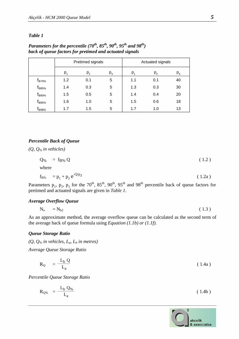
Table 1

Parameters for the percentile (70th, 85th, 90th, 95th and 98th) back of queue factors for pretimed and actuated signals

Pretimed signals Actuated signals

p1 p2 p3 p1 p2 p3

fB70% 1.2 0.1 5 1.1 0.1 40

fB85% 1.4 0.3 5 1.3 0.3 30

fB90% 1.5 0.5 5 1.4 0.4 20

fB95% 1.6 1.0 5 1.5 0.6 18

fB98% 1.7 1.5 5 1.7 1.0 13

Percentile Back of Queue (Q, Q% in vehicles)

Q% = fB% Q ( 1.2 )

where

fB% = p1 + p2 e-Q/p3 ( 1.2a )

Parameters p1, p2, p3 for the 70th, 85th, 90th, 95th and 98th percentile back of queue factors for pretimed and actuated signals are given in Table 1.

Average Overflow Queue No = Nb2 ( 1.3 )

As an approximate method, the average overflow queue can be calculated as the second term of the average back of queue formula using Equation (1.1b) or (1.1f).

Queue Storage Ratio (Q, Q% in vehicles, La, Lh in metres)

Average Queue Storage Ratio

RQ = L

Q L

a

h ( 1.4a )

Percentile Queue Storage Ratio

RQ% = L

Q L

a

%h ( 1.4b )


where

Lh is the jam spacing (average spacing in a stationary queue) in metres,

La is the available queue storage distance in metres,

Q is the average back of queue (vehicles per lane), Q% is the percentile back of queue (vehicles per lane).

The available queue storage distance can be calculated as the blocking queue distance, which is the distance from the downstream stop line to the back of downstream queue that blocks the upstream stop line.

Queue Clearance (Service) Time (sLg in vehicles, gs, r in seconds)

gs = – y1

ryf

L

Lq subject to gs ≤ g ( 1.5 )

fq = PF2 for pretimed signals ( 1.5a )

= PF2 [1.08 - 0.1 (G/Gmax)2 ] for actuated signals ( 1.5b ) subject to [1.08 - 0.1 (G/Gmax)2 ] ≥ 1.0

PF2 is the queue progression factor.

Model Parameters (sLg, QbL in vehicles , T in hours, cL in veh/h, v, vL, s, sL in veh/h)

Adjusted Flow Rate and Flow Ratio

vL = vl / NLG = (v + Qb / T) / NLG = v / NLG + QbL / T ( 1.6a )

yL = vL / sL = (v / NLG + QbL / T) / sL = (v / s) + QbL / (sL T) ( 1.6b )

(vL = v / NLG and yL = v / s for zero initial queued demand, QbL = 0)

Degree of Saturation

XL = vL / cL = (v / NLg + QbL / T) / cL = (v / c) + QbL / (cL T) ( 1.7 )

= X + QbL / (cL T)

(XL = X for zero initial queued demand, QbL = 0)

X = v / c ( 1.7a )


Second term parameter

z = X - 1 + Tc

Q2

L

bL = (XL -1) + Tc

Q

L

bL ( 1.8 )

(z = X – 1 = XL -1 for zero initial queued demand, QbL = 0)

Average Values per Lane

The demand flow rate (vL), saturation flow rate (sL), capacity per cycle (sLg), capacity (cL) and initial queued demand (QbL) in Equations (1.1) to (1.8) should be used as individual lane values, or when applying the equations on a lane group basis, average values per lane should be used. These can be calculated from:

vL = vl / NLG = (v + Qb / T) / NLG ( 1.9a )

sL = s / NLG ( 1.9b )

cL = c / NLG ( 1.9c )

QbL = Qb / NLG ( 1.9d )

where vl and v are the total flow rates for the lane group with and without the effect of initial queued demand, s, c and Qb are the total saturation flow rate, capacity and initial queued demand for the lane group, and NLG is number of lanes in the lane group.

A refinement for the case of unequal lane utilisation is described in Appendix B.

Queue Progression Factor

The progression factors apply to the case of platooned arrivals generated by coordinated signals. For more detailed information on progression factors, refer to Akçelik (1995, 1996, 2001). The Queue Progression Factor (PF2) is calculated from:

PF2 = )yR1()u1(

)y1()P1(

Lp

L−−

−− = )yR1()u1()y1()uR1(

Lp

Lp−−

−− ( 1.10 )

subject to conditions (i) PF2 ≥ 1.0 for Arrival Types 1 and 2, (ii) PF2 ≤ 1.0 for Arrival Types 4 to 6, (iii) P ≤ 1.0 (Rp ≤ 1 / u), (iv) Rp < 1 / yL, and (v) PF2 = 1.0 for yL ≥ u (XL ≥ 1).

where u is the green time ratio (g/C), yL is the lane group flow ratio per lane, i.e. vL/sL ratio where vL is the lane group flow rate per lane (veh/h) and sL is the lane group saturation flow rate per lane (veh/h), and Rp is the platoon ratio:

Rp = vLg / vL = P / u ( 1.10a )


where vLg is the arrival flow rate per lane (veh/h) during the green period (vLg = Rp vL), vL is the average arrival flow rate per lane (veh/h) during the signal cycle, and P is the proportion of traffic arriving during the green period.

If the user specifies a known value of P rather than an Arrival Type, then Rp = P / u can be calculated and used to determine a corresponding arrival type (see Akçelik 2001, Table 1).

For non-platooned (uniform) arrivals as relevant to isolated intersections, use Rp = 1.0, therefore:

PF2 = 1.0 and ( 1.11 ) If = 1.0

Various cases

Two green periods per cycle

In the case of two green periods per cycle (e.g. a turning movement that receives a green circle and a green arrow, i.e. permitted and protected turns in HCM terminology):

(i) in the formula for fq, (G/Gmax)i values are used for the relevant green periods individually (i = 1, 2),

(ii) for the second-term parameter kB, the total sLg per cycle is used: sLg = (sLg)1 + (sLg)2, and

(iii) uniform back of queue and queue clearance time models need to be extended to include any residual queues from the previous green period (as in aaSIDRA).

Queue accumulation polygons used in HCM 2000 Chapter 16, Appendix B could be extended for queue prediction in the case of two green periods in future editions of HCM.

Permitted (filter) turns in a shared lane

In the formula for fq, (G/Gmax) value of the through movement is normally used in the case of permitted (filter) turns in a shared lane. In the case of permitted and protected turns from a shared lane, (G/Gmax) value of the through movement is used for the permitted (filter) turn period.


Model Validation Comparisons of various model estimates with simulation and real-life data are discussed in this section. All cases are for isolated intersection conditions (random arrivals).

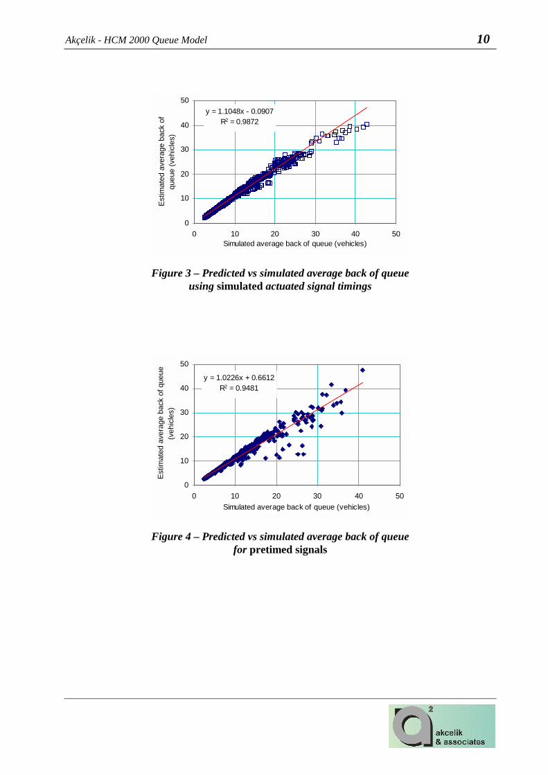
Comparison of average back of queue estimates from the proposed model (Equation 1.1) against actuated and fixed-time signal simulation data generated using ModelC (Akçelik and Chung 1994, 1995a,b, Akçelik, Chung and Besley 1997, Akçelik, Besley and Chung 1998) is given in Figures 2 to 4. The closeness of results using the estimated and simulated actuated signal timings (Figures 2 and 3) indicates the accuracy of the actuated signal timing method introduced in HCM 97 (Courage, et al 1996).

Comparison of average back of queue estimates from the proposed model for actuated signals against back of queue values measured at an in intersection in Melbourne, Australia (using measured signal timings) is shown in Figure 5.

Comparison of average back of queue estimates from the proposed model and the aaSIDRA model for the same site is shown in Figure 6.

Slight overestimation of queue length by the proposed and aaSIDRA back of queue models is acceptable because the analytical models include vehicles slowing down at the back of queue without coming to a full stop whereas field surveys are likely to have undercounted such vehicles.

A paper by Viloria, Courage and Avery (2000) presented a detailed discussion on the HCM 2000 queue model and comparisons with the aaSIDRA and various other queue models for signalised intersections.

y = 1.1788x - 0.8943R2 = 0.9835

0

10

20

30

40

50

0 10 20 30 40 50Simulated average back of queue (vehicles)

Estim

ated

ave

rage

bac

k of

qu

eue

(veh

icle

s)

Figure 2 – Predicted vs simulated average back of queue using estimated actuated signal timings


y = 1.1048x - 0.0907R2 = 0.9872

0

10

20

30

40

50


Estim

ated

ave

rage

bac

k of

qu

eue

(veh

icle

s)

Figure 3 – Predicted vs simulated average back of queue using simulated actuated signal timings

y = 1.0226x + 0.6612R2 = 0.9481

0

10

20

30

40

50


Estim

ated

ave

rage

bac

k of

que

ue

(veh

icle

s)

Figure 4 – Predicted vs simulated average back of queue for pretimed signals


y = 1.2414x - 1.0717R2 = 0.9757

0.0

4.0

8.0

12.0

16.0

20.0

24.0

0 4 8 12 16 20 24

Average back of queue (veh) (Manual survey)

Aver

age

back

of q

ueue

(veh

) (H

CM

200

0 es

timat

e)

Figure 5 – Comparison of average back of queue values predicted by the proposed model with those measured at an isolated intersection controlled by actuated signals in Melbourne,

Australia (using measured timings)

y = 1.1078x - 0.5481R2 = 0.9991

0.0

4.0

8.0

12.0

16.0

20.0

24.0

0 4 8 12 16 20 24

Average back of queue (veh) (SIDRA estimate)

Aver

age

back

of q

ueue

(veh

) (H

CM

200

0 es

timat

e)

Figure 6 – Comparisons of average back of queue estimates from the proposed model and the SIDRA model for the same site as in Figure 5


Large Values of Back of Queue

A frequently asked question by aaSIDRA users who have not been familiar with the back of queue concept (due to the lack of this concept from the HCM editions prior to HCM2000) is related to the large size of queue length that the model can produce. The following issues should be considered in this respect.

(i) Back of queue vs cycle-average queue: Back of queue is always larger than the more familiar cycle-average queue. The latter is calculated using average delay (e.g. as in the HCM unsignalised intersections chapter), and as such, incorporates all queue states including zero queues, resulting in a smaller value than the back of queue.

(ii) Progression effects: As discussed in Akçelik (2001), very poor and unfavourable progression conditions result in queue lengths that may be considerably larger than those under random arrival conditions.

(iii) Percentile queue length: If a percentile queue length is used this could be as high as twice or three times the average queue length. However, percentile queues occur only a limited number of times during the analysis period. For example, the 90th percentile back of queue is exceeded only in 10 per cent of the signal cycles. With a cycle time of C =100 s, there are 9 signal cycles in the peak analysis period of 15 minutes used in the HCM. In this case, the 90th percentile back of queue is exceeded 0.9 times (say once) during the analysis period.

(iv) Arrival (demand) flow rate: Delay and back of queue are not always consistent in terms of magnitude. Low average delay can be associated with a long back of queue (as seen in Figure 7) as a result of a high arrival flow rate, large green time ratio (relatively short red period) and low degree of saturation. In this case, a large proportion of vehicles may be undelayed, and therefore the cycle-average queue could be small. In contrast, the case of short back of queue may be associated with a large average delay (as seen in Figure 8) as a result of a low arrival flow rate, small green time ratio (relatively long red period) and a high degree of saturation.

In Figure 7, vehicles are seen to arrive during the red period and the early part of the green period, which represents platooned arrivals with unfavourable progression. Therefore it corresponds to the case of large progression factors discussed in Akçelik (2001).

A clear understanding of the above issues is needed for effective use of delay and queue length as interrelated performance measures for signalised intersections.


Back of queue

r g

Delay

Arriving vehicles

C

Departing vehicles

Time

Distance from stop line

Figure 7 - The case of low delay associated with a long back of queue (high arrival flow rate, large green time ratio, and low degree of saturation)

Back of queue

r g

Delay

Arriving vehicles

C

Departing vehicles

Time

Distance from stop line

Figure 8 - The case of short back of queue associated with a large average delay (low arrival flow rate, small green time ratio, and high degree of saturation)


Notations and Basic Relationships

HCM 2000 and this document

aaSIDRA and original document

c Lane group capacity (veh/h) c = s g / C (where s is in veh/h)

cL Qe Lane group capacity per lane (veh/h) cL = c / NLG = sL g / C where sL = s / NLG

cL T Qe Tf Lane group throughput per lane (maximum number of vehicles that can be discharged during the flow period)

C c Average cycle time (seconds) C = r + g

fB% fbp% Percentile back of queue factor

fLU Saturation flow adjustment factor for unequal lane utilisation

fq fq Calibration factor for queue clearance time

g g Average effective green time (seconds)

g/C, u u Green time ratio u = g / C

gs, gq gs Average queue clearance (service) time, or saturated portion of the green period (seconds)

gu gu Unsaturated portion of the green period (seconds) gu = g – gs

I If Upstream filtering factor for platooned arrivals

kB kb Incremental queue factor (similar to "k" in the HCM delay formula)

La La Available queue storage distance (lane length in metres)

Lh Lhj Average spacing in a stationary queue including the vehicle length and the gap distance in front of the vehicle (jam spacing) (m/veh)

NLG nLG Number of lanes in the lane group (to determine the critical lane flow rate, use fLU NLG as an effective number of lanes instead of NLG)

P PG Proportion of traffic arriving during the green period P = Rp u

continued >>>




PF2 PF2 Progression factor for back of queue and queue clearance time

Q Nb Average back of queue (vehicles)

Q1, Q2 Nb1, Nb2 First and second terms of the average back of queue formula

Q% Nbp% Percentile (70th, 85th, 90th, 95th, or 98th) value of the back of queue

QbL Ni Initial queued demand per lane as observed at the start of a flow period (vehicles)

Qb Initial queued demand for the lane group as observed at the start of a flow period (vehicles)

Qd (not in HCM)

Nd Deterministic oversaturation queue assuming constant demand and capacity flow rates and ignoring the first-term queue

Qo (not in HCM)

No Average overflow queue

No = Nb2 as an approximate method

r r Average effective red time (seconds) r = C – g

Rp PA Platoon arrival ratio for coordinated signals: the ratio of the average arrival flow rate during the green period to the average arrival flow rate during the signal cycle

Rp = P / u

RQ Rq Average queue storage ratio: the ratio of the average back of queue (distance) to the available queue storage distance

RQ = Lh Q / La

RQ% Rqp% Percentile queue storage ratio: the ratio of the percentile value of the back of queue (distance) to the available queue storage distance

RQ% = Lh Q% / La

s Lane group saturation flow rate (veh/h)

sL s Lane group saturation flow rate per lane (veh/h) sL = s / NLG

sLg sg Cycle capacity per lane (veh) (sL in veh/s, g in seconds)

T Tf Duration of a demand flow (analysis) period (hours)

continued >>>




v qa Arrival (demand) flow rate (veh/s or veh/h), i.e. the average number of vehicles per unit time as measured at a point upstream of the back of queue (without the effect of the initial queued demand)

vl qai Demand flow rate adjusted to take into account the initial queued demand at the start of the flow period

vl = v + Qb / T

vL Lane group arrival (demand) flow rate per lane including the effect of initial queued demand (veh/h)

vL = vl / NLG = (v + Qb / T) / NLG = v / NLG + QbL / T if there is no initial queued demand, Qb = 0, vL = v / NLG

vL C qai c Average demand (vehicles) per lane per cycle corresponding to the total demand including initial queued demand

X x Lane group degree of saturation, i.e. the ratio of arrival (demand) flow rate to capacity (without the effect of the initial queued demand)

X = v / c = (v/NLG) / cL

XL x' Lane group degree of saturation per lane, i.e. the ratio of arrival (demand) flow rate to capacity including the effect of the initial queued demand

XL = vL / cL = vL C / (sL g) = yL / u = (v / NLg + QbL / T) / cL = X + QbL / (cL T) if there is no initial queued demand, QbL = 0, XL = X

Xu xu Degree of saturation at the upstream intersection (used for upstream filtering factor I). HCM 2000 Chapter 15 qualifies this as the flow weighted average of contributing upstream movement v/c ratios.

yL y Lane group flow ratio per lane, i.e. the ratio of arrival (demand) flow rate to the saturation flow rate including the effect of the initial queued demand

yL = vL / sL = u XL if there is no initial queued demand, Qb = 0, yL = v / s

z (not in HCM)

z A performance model parameter used in the second term of the back of queue expression

z = X – 1 + 2 QbL / (cL T) = (XL - 1) + QbL / (cL T) if there is no initial queued demand, QbL = 0, z = X – 1


REFERENCES

AKCELIK & ASSOCIATES (2000). aaSIDRA User Guide. Akcelik and Associates Pty Ltd, Melbourne, Australia. AKÇELIK, R. (1980a). Time-Dependent Expressions for Delay, Stop Rate and Queue Length at Traffic Signals. Internal Report AIR 367–1. Australian Road Research Board, Vermont South, Australia.

AKÇELIK, R. (1980b). Stops at traffic signals. Proc. 10th ARRB Conf. 10(4), pp. 182-192, 1980.

AKÇELIK, R. (1981). Traffic Signals: Capacity And Timing Analysis. Research Report ARR No. 123. ARRB Transport Research Ltd, Vermont South, Australia. (6th reprint: 1995).

AKÇELIK, R. (1984). SIDRA-2 does it lane by lane. Proc. 12th ARRB Conf. 12 (4), pp. 137-149.

AKÇELIK, R. (1988a). Capacity of a shared lane. Proc. 14th ARRB Conf. 14 (2), pp. 228-241.

AKÇELIK, R. (1988b). The Highway Capacity Manual delay formula for signalised intersections. ITE Journal, 58 (3), pp. 23-27.

AKÇELIK, R. (1989). On the estimation of lane flows for intersection analysis. Aust. Rd Res. 19 (1), pp. 51-57.

AKÇELIK, R. (1990a). Calibrating SIDRA. Research Report ARR No. 180. ARRB Transport Research Ltd, Vermont South, Australia. (2nd edition, 1st reprint 1993).

AKÇELIK, R. (1990b). SIDRA for the Highway Capacity Manual. Compendium of Technical Papers. 60th Annual Meeting of the Institute of Transportation Engineers, Orlando, Florida, pp. 210–219.

AKÇELIK, R. (1995). Extension of the Highway Capacity Manual Progression Factor Method for Platooned Arrivals. Research Report ARR No. 276. ARRB Transport Research Ltd, Vermont South, Australia.

AKÇELIK, R. (1996). Progression factor for queue length and other queue-related statistics. Transportation Research Record 1555, pp 99-104.

AKÇELIK, R. (1997). Lane-by-lane modelling of unequal lane use and flares at roundabouts and signalised intersections: the SIDRA solution. Traffic Engineering and Control, 38 (7/8), pp. 388-399..

AKÇELIK, R. (1998). A Queue Model for HCM 2000. Technical Note. ARRB Transport Research Ltd, Vermont South, Australia. AKÇELIK, R. (2001). Progression Factors in the HCM 2000 Queue and Delay Models for Traffic Signals. Technical Report. Akcelik and Associates Pty Ltd, Melbourne, Australia.

AKÇELIK, R., BESLEY M. and CHUNG, E. (1998). An evaluation of SCATS Master Isolated control. Proceedings of the 19th ARRB Transport Research Conference (Transport 98) (CD), pp 1-24. ARRB Transport Research Ltd, Vermont South, Australia.


AKÇELIK, R., CHUNG, E. and BESLEY, M. (1998). Roundabouts: Capacity and Performance Analysis. Research Report ARR No. 321. ARRB Transport Research Ltd, Vermont South, Australia.

AKÇELIK, R. and CHUNG, E. (1994). Traffic performance models for unsignalised intersections and fixed-time signals. In: Akçelik, R. (Ed.), Proceedings of the Second International Symposium on Highway Capacity, Sydney, 1994, ARRB Transport Research Ltd, Vermont South, Australia, Volume 1, pp. 21-50.

AKÇELIK, R. and CHUNG, E. (1995a). Calibration of Performance Models for Traditional Vehicle-Actuated and Fixed-Time Signals. Working Paper WD TO 95/013. ARRB Transport Research Ltd, Vermont South, Australia.

AKÇELIK, R. and CHUNG, E. (1995b). Delay Model for Actuated Signals. Technical Note WD TO 95/013-A. ARRB Transport Research Ltd, Vermont South, Australia.

AKÇELIK, R., CHUNG, E. and BESLEY M. (1997). Recent research on actuated signal timing and performance evaluation and its application in SIDRA 5. Compendium of Technical Papers (CD). 67th Annual Meeting of the Institution of Transportation Engineers, Boston, USA.

AKÇELIK, R. and ROUPHAIL, N.M. (1994). Overflow queues and delays with random and platooned arrivals at signalised intersections. Journal of Advanced Transportation, 28 (3), pp. 227-251.

COURAGE, K.G, FAMBRO, D.B., AKÇELIK, R., LIN, P-S., ANWAR, M. and VILORIA, F. (1996). Capacity Analysis of Traffic Actuated Intersections. NCHRP Project 3-48 Final Report Prepared for National Cooperative Highway Research Program, Transportation Research Board, National Research Council. KIMBER, R. M. and HOLLIS, E. M. (1979). Traffic Queues and Delays at Road Junctions. Transp. Road Res. Lab. (U.K.) TRRL Lab. Report LR 909.

MILLER, A. J. (1968). Signalised Intersections - Capacity Guide. Bulletin No. 4. Australian Road Research Board, Vermont South, Australia.

TARKO, A. and RAJARAMAN, G. (1998). In: Third International Symposium on Highway Capacity, Copenhagen, Denmark, 22-27 June 1998, Volume 1 (Edited by R. Rysgaard). Road Directorate, Ministry of Transport, Denmark, pp. 1007-1025.

VILORIA, F., COURAGE, K. and AVERY, D. (2000). Comparison of queue length models at signalised intersections. Paper presented at the 79th Annual Meeting of the Transportation Research Board, Washington, D.C., U.S.A.

TRB (1998). Highway Capacity Manual. Special Report 209. Transportation Research Board, National Research Council, Washington, D.C., U.S.A. (“HCM 1997”).

TRB (2000). Highway Capacity Manual. Transportation Research Board, National Research Council, Washington, D.C., U.S.A. (“HCM 2000”).

WEBSTER, F. V. (1958). Traffic Signal Settings. Road Res. Lab. Tech. Paper No. 39. HMSO, London.


Appendix A

Background to the Development of the HCM 2000 Back of Queue Model

The HCM 2000 second-term back of queue model is a time-dependent expression. This means that the queue length predicted by this expression depends on the duration of the analysis period, which represents how long the demand flow rate persists (HCM 2000 default is 15 minutes). In contrast, earlier forms of the delay and queue models in the literature are based on steady-state conditions, i.e. they assume that flow conditions last indefinitely (Webster 1958, Miller 1968). Time-dependent expressions are derived from steady-state expressions using a well-known coordinate transformation technique (Kimber and Hollis 1979, Akçelik 1980a). The principles of the discussion below are applicable to delay as well (Akçelik 1980a,b, 1981, 1988b, 1990a,b, Akçelik and Rouphail 1994).

Time-dependent and steady-state forms of a model predict close values for low degrees of saturation but differ as demand flows approach capacity. A steady-state model is valid only for demand flow rates below capacity, say for degrees of saturation up to about 0.95. A time-dependent model predicts the same values as its steady-state counterpart when a very large value of the analysis period is used.

The origin of the HCM 2000 second-term queue expression can be traced back to the time-dependent model developed by the author (Akçelik 1980a,b, 1981) using an approximation to the steady-state form of the overflow queue model described by Miller (1968). This is explained below using time-dependent expressions without initial queued demand.

Miller's overflow queue model for pretimed signals is given by:

Qos = )X1(2

]X/)X1()6003/gs(33.1[exp

L

LL5.0

L−

−− ( A.1 )

where Qos is the average overflow queue in steady-state form (subscript s is used to denote steady-state), sLg is the capacity per cycle in vehicles (sL = lane group saturation flow rate per lane in veh/h, g = effective green time in seconds), and XL is the lane group degree of saturation (demand volume/capacity ratio). In order to facilitate the derivation of a time-dependent function for the average overflow queue, the author developed the following general steady-state model for undersaturated signals using the general structure of Miller's formula that predicts negligible values of overflow queue for low degrees of saturation:

Qos = L

oLoX1

)XX(k−

− for XL > Xo ( A.2 )

= 0 otherwise where ko is the overflow queue parameter, XL is the degree of saturation, and Xo is a degree of saturation below which the average overflow queue is zero.

As an approximation to Equation (A.1), the following parameter values were used in Equation (A.2):


ko = 1.5 , and Xo = 0.67 + 600

3600/gsL ( A.2a )

where sLg/3600 is the cycle capacity (vehicles). These parameters are for pretimed signals. For the derivation of the time-dependent form of the overflow queue expression, a deterministic oversaturation queue (Qd) model is also needed. This is derived by assuming constant arrival flow rate (vL) and constant capacity (cL) over an analysis period (T), where vL > cL, therefore XL = vL / cL > 1.0:

Qd = 0.5 (XL – 1) T ( A.3 ) Overflow queues estimated by steady-state expressions (Equations A.1, A.2 and A.2a) for undersaturated conditions and the deterministic expression (Equation A.3) for oversaturated conditions are shown in Figure A.1. This figure is based on the following example: no initial queued demand, pretimed signals with no signal coordination effects (Arrival Type = 3), green time, g = 40 s, cycle time, C = 100 s, saturation flow rate, sL = 1800 veh/h, therefore cycle capacity, sLg = 20 veh, capacity, cL = 720 veh/h, and analysis period, T = 0.25 h. Limitations of steady-state and deterministic oversaturation queue expressions are indicated in Figure A.1. While the deterministic expression predicts a zero overflow queue value at capacity (degree of saturation, XL < 1.0), the steady-state expressions predict infinite overflow queue values for flows just below capacity (XL > 1.0). Thus, these equations do not give reasonable results for flows near capacity. The problem is solved using the coordinate transformation technique to convert the steady-state function to a transition function that has the line representing the deterministic function as its asymptote. The result is a time-dependent expression that gives realistic finite values of the overflow queue (or delay) for flows around capacity, and adds a random component to the deterministic oversaturation function. The time-dependent function for the average overflow queue obtained using the coordinate transformation technique to relate Equations (A.2) and (A.2a) to Equation (A.3) is shown in Figure A.1.

0

2

4

6

8

10

0.40 0.50 0.60 0.70 0.80 0.90 1.00 1.10 1.20


Aver

age

over

flow

que

ue (v

eh)

Deterministic

Steady-state (Miller)

Steady-state (Akcelik)

Time-dependent (Akcelik)

Figure 1 - The relationship between the time-dependent, steady-state and deterministic

oversaturation models for overflow queue prediction


Similarly, the steady-state model that is the basis of the HCM 2000 back of queue model (second-term) is given by:

Q2s = L

LBX1Xk

− ( A.4 )

where kB is the back of queue model parameter (HCM 2000 Equation G16-10) and XL is the degree of saturation. Comparing Equations (A.2) and (A.4), it is seen that and Xo = 0 in Equation (A.4), and kB replaces parameter ko.

The second-term of the HCM 2000 back of queue model (HCM 2000 Equation G16-9) is a time-dependent model based on Equation (A.4). When there is no initial queued demand, this is given by:

Q2 = 0.25 cL T [z + (z2 + Tc Xk8

L

Lb )0.5] ( A.5 )

where cL = lane group capacity per lane, T = analysis period, z = XL - 1, and XL = degree of saturation.

Figure A.2 shows how the HCM 2000 second-term model (Equation A.5) relates to the corresponding steady-state model (Equation A.4) and the deterministic oversaturation queue model (Equation A.3) for the same example as in Figure A.1.

0

2

4

6

8

10

12

14

0.00 0.20 0.40 0.60 0.80 1.00 1.20


Seco

nd-te

rm b

ack

of q

ueue

(veh

)

Deterministic

Steady-state (HCM2000)

Time-dependent (HCM2000)

Figure 2 - The relationship between the HCM2000 second-term back of queue model (time-

dependent), and the corresponding steady-state and deterministic oversaturation models


Figure A.3 shows a comparison of the average back of queue values (Q = Q1 + Q2) calculated using the HCM 2000 model, its "parent model" used in aaSIDRA (Viloria, Courage and Avery 2000), and the earlier model based on the use of parameters given in Equation (A.2b) for the same example as in Figures A.1 and A.2. The first-term back of queue results (Q1) for the HCM model are also shown in Figure A.3.

It is seen that the HCM 2000 and aaSIDRA second-term queue models give larger values than the earlier model. This is mainly due to different assumptions in arrival headway distributions (bunched exponential rather than simple negative exponential). For the example shown in Figure A.3, the first-term queue expression makes a larger contribution to the average back of queue for undersaturated conditions, and therefore the differences in the second-term expressions are less important.

0

5

10

15

20

25

30

35

40

0.00 0.20 0.40 0.60 0.80 1.00 1.20


Aver

age

back

of q

ueue

(veh

)

HCM2000

aaSIDRA

Akcelik early model

First-term back of queue

Figure 3 - Comparison of the average back of queue values predicted by the HCM2000,

aaSIDRA and an earlier model


Appendix B

A Method for Determining Model Parameters in the Case of

Unequal Lane Utilisation

The following method is recommended for determining the back of queue in the critical lane of a lane group with unequal lane utilisation. This method has a shortcoming due to the assumption of equal lane saturation flows, which can only be overcome using a lane-by lane analysis method as in aaSIDRA (Akcelik and Associates 2000; Akçelik 1984, 1988a, 1989, 1997; Akçelik, Chung and Besley 1998).

From Equations (1.9a) to (1.9d) in the main text of this report (corresponding to Equations G16-2 to G16-5 of HCM 2000), the lane group arrival flow rate (vL), saturation flow rate (sL), capacity (cL) and initial queued demand (QbL) per lane in the case of equal lane utilisation are:

vL = vl / NLG ( B.1 )

sL = s / NLG ( B.2 )

cL = c / NLG ( B.3 )

QbL = Qb / NLG ( B.4 )

where vl is the total flow rate for the lane group with the effect of initial queued demand, s, c and Qb are the total saturation flow rate, capacity and initial queued demand for the lane group, and NLG is number of lanes in the lane group.

The total flow rate for the lane group with the effect of initial queued demand (Qb) is:

vl = v + Qb / T ( B.5 )

where v is the total flow rate for the lane group without the effect of initial queued demand, and T is the duration of the demand flow (analysis) period.

The method given here is applicable to the case of no initial queued demand (Qb = 0 and vl = v).

On the basis of HCM 2000, Exhibit 16-7, the adjustment factor for lane utilisation can be expressed as:

fLU = vl / (vc NLG) ( B.6 )

where vl is as in Equations (B.1) and (B.5), and vc is the corresponding flow rate for the critical lane in the lane group.

From Equations (B.1) and (B.6), the lane utilisation factor is equivalent to the ratio of the average lane flow rate to the critical lane flow rate:

fLU = vL / vc ( B.6a )


Thus, the critical lane flow is given by:

vc = vl / (fLU NLG) = vL / fLU ( B.7 )

Assuming the same lane saturation flow for all lanes in the same group (si), including the critical lane, the lane group saturation flow is:

s = NLG si fLU ( B.8 )

In terms of HCM 2000 Equation 16-4 (see HCM 2000 for symbols), the lane saturation si is equivalent to:

si = so fw fHV fg fp fbb fa fLT fRT fLpb fRpb ( B.8a )

Since the critical lane saturation flow is sc = si (the same for all lanes), Equations (B.8) and (B.2) imply:

sc = s / (fLU NLG) = sL / fLU ( B.9 )

The critical lane flow ratio is:

yc = vc / sc = (vL / fLU) / (sL / fLU) = vL / sL = yL ( B.10 )

It is seen that the flow ratio obtained using the average flow rate and saturation flow rate per lane is the same as the critical lane flow ratio (yL = yc).

The critical lane capacity is:

cc = sc g / C = (s / (fLU NLG)) g / C = c / (fLU NLG) = cL / fLU ( B.11 )

The critical lane degree of saturation is:

Xc = vc / cc = (vL / fLU) / (cL / fLU) = vL / cL = XL ( B.12 )

It is seen that the degree of saturation obtained using the average flow rate and capacity per lane is the same as the critical lane degree of saturation (XL = Xc).

Assuming that the initial queued demand in each individual lane is proportional to the lane flow, the initial queued demand for the critical lane is given by:

Qbc = Qb / (fLU NLG) = QbL / fLU ( B.13 )

It should also be noted that the HCM 2000 method implies equal arrival flow rates for non-critical lanes (for NLG > 2):

vn = (vl - vc) / (NLG - 1) ( B.14 )

In summary, parameters for the back of queue equation in the case of unequal lane utilisation case can be calculated by replacing NLG in Equations G16-2 to G16-5 of HCM 2000 by (fLU NLG) as an effective number of lanes.

vL = vl / (fLU NLG) ( B.15 )

sL = s / (fLU NLG) ( B.16 )


cL = c / (fLU NLG) ( B.17 )

QbL = Qb / (fLU NLG) ( B.18 )

Equations (B.1) to (B.4) can be considered to be a special case of Equations (B.15) to (B.18), valid only when fLU = 1.0.

Example: Consider a lane group with three lanes (NLG = 3), a total flow rate of v = 1095 veh/h, lane saturation flow rate of si = 1800 veh/h, initial queued demand of Qb = 30 vehicles, demand flow period of T = 0.25 h, and a lane utilisation factor of fLU = 0.8333. Effective green time and cycle time are g = 30 s and C = 100 s.

The total flow rate for the lane group with the effect of initial queued demand is vl = 1095 + 30/ 0.25 = 1215 veh/h. The saturation flow rate for the lane group is s = 3 x 1800 x 0.8333 = 4500 veh/h. The lane group capacity is c = 4500 x 30 / 100 = 1350 veh/h. The degree of saturation using the flow rate with the effect of the initial queued demand is 1215 / 1350 = 0.900. The flow ratio using the flow rate with the effect of the initial queued demand is 1215 / 4500 = 0.270.

The effective number of lanes to allow for lane underutilisation is fLU NLG = 0.8333 x 3 = 2.5 lanes. Using this, the parameters required on a per lane basis (reflecting the critical lane conditions rather than average lane conditions) are calculated from Equations (B.15) to (B.18):

vL = vc = 1215 / 2.5 = 486 veh/h per lane sL = sc = 4500 / 2.5 = 1800 veh/h per lane = si cL = cc = 1350 / 2.5 = 540 veh/h per lane QbL = Qbc = 30 / 2.5 = 12 veh per lane

The degree of saturation and flow ratio for the critical lane for use in the back of queue equations are:

XL = Xc = 486 / 540 = 0.900 (as for the lane group) yL = yc = 486 / 1800 = 0.270 (as for the lane group)

It is seen that the critical lane and the lane group have the same degree of saturation and the same flow ratio. This is achieved through the use of the lane utilisation adjustment factor (fLU) in the saturation flow formula.

For the second-term back of queue equation, we also need the degree of saturation using the flow rate without the effect of initial queued demand. On a lane group basis, X =v /c = 1095 / 1350 = 0.811. This can also be calculated for the critical lane:

vc = 1095 / 2.5 = 438 veh/h per lane X = 438 / 540 = 0.811 (as for the lane group).

For this example, Equations (1.1a) and (1.1b) give Q1 = 12.95 veh, Q2 = 6.94 veh, therefore Q = 19.9 veh. HCM 2000 Equation G16-9 underestimates the second term, Q2 = 4.96 veh, therefore Q = 17.9 veh.

HCM 2000 Back of Queue Model for Signalised Intersections · 2007-06-25 · A major improvement in...

Documents

Transcript of HCM 2000 Back of Queue Model for Signalised Intersections · 2007-06-25 · A major improvement in...