HBNI Th44 TCS.pdf
175
THE KERNELIZATION COMPLEXITY OF SOME DOMINATION AND COVERING PROBLEMS G P e Institute of Mathematical Sciences, Chennai, India. A thesis submitted to the Board of Studies in Mathematical Sciences in partial fullment of the requirements for the Degree of Doctor of Philosophy of Homi Bhabha National Institute September
Transcript of HBNI Th44 TCS.pdf
THE KERNELIZATION COMPLEXITY OF SOME
DOMINATION AND COVERING PROBLEMS
Geevarghese Philip
e Institute of Mathematical Sciences, Chennai, India.
A thesis submitted to the
Board of Studies in Mathematical Sciencesin partial fullment of the requirements
for the Degree of
Doctor of Philosophyof
Homi Bhabha National Institute
September 2011
e Kernelization Complexity of Some Domination and Covering Problems, PhDesis.
© Geevarghese Philip, September 2011.cbna Licensed under a Creative Commons
Attribution-NonCommercial-ShareAlike 2.5 India License
To Manju Joseph, my wife.
To A. P. Geevarghese and Saramma Philip, my parents.

Abstract
Polynomial-time preprocessing is a simple algorithmic strategy which has been
widely employed in practice to tackle hard problems. e quantication and
analysis of the eciency of preprocessing algorithms are, in a certain precise
sense, outside the pale of classical complexity theory.e notion of kernelization from
parameterized complexity theory provides a framework for the mathematical analysis of
polynomial-time preprocessing algorithms. Both kernelization and the closely related
notion of xed-parameter tractable (FPT) algorithms are very active areas of current
research. In this thesis we describe the results of our study of the kernelization complexity
of some graph domination and covering problems.
An instance of a parameterized problem is of the form (x , k) where x is a classical
problem instance and k is a suitably-chosen parameter. A xed-parameter tractable (FPT)
algorithm for the problem is an algorithm which solves the problem in timeO( f (k) ⋅ ∣x∣c)
for some computable function f () and constant c. A kernelization algorithm for the
problem is a polynomial-time algorithm which converts the input instance (x , k) to an
equivalent parameterized instance (x′, k′) where both the size of the new instance x′ and
the value of the new parameter k′ are bounded by some computable function f (k) of the
original parameter k.e new instance is called a kernel for the problem, and f (k) is the
size of the kernel. In the following, n denotes the number of vertices in the input graph,
and k is the parameter in each case.
e study of variants of the domination problem in graphs has been a vibrant area
of research for many decades, and continues to be a rich source of graph-theoretical
and algorithmic problems.e prototypical problem in this eld is Dominating Set, a
classical minimization problem which asks whether the input graph has a dominating
v
set of size at most k.e natural parameterization of this problem— with the solution
size k as the parameter (Parameterized Dominating Set) — is known to be W[2]-
complete, and hence is unlikely to have an FPT algorithm on general graphs. We begin
our study of the kernelization complexity of graph domination problems by showing
that for every xed j ≥ i ≥ 1, the Parameterized Dominating Set problem is FPT
and has a polynomial kernel on graphs that do not have the complete bipartite graph
Ki , j as a subgraph. In particular, this implies that the problem has polynomial kernels
on graphs of bounded degeneracy. We then consider a variant of the Dominating Set
problem, named Connected Dominating Set, where the dominating set is required
to be connected.e natural parameterized version of this problem (Parameterized
Connected Dominating Set) is also known to be W[2]-complete on general graphs.
We study the eect of the girth of the input graph on the kernelization complexity of this
problem, and discover an interesting scenario : the problem is W[2]-hard on graphs of
girth 3 or 4, is FPT on graphs of girth at least 5, is unlikely to have polynomial-size kernels
on graphs of girth 5 or 6, and has a polynomial kernel on graphs of girth at least 7.
We nowmove on to the study of various graph covering problems, where the objective
is to nd a small subset of vertices and/or edges of the input graph such that their removal
deletes certain specied structures from the graph.e rst problem we consider is the
Parameterized Pathwidth-One Vertex Deletion problem which asks whether one
can delete at most k vertices from the input graph such that the remaining graph has
pathwidth at most one; the parameter is k. A graph has pathwidth at most one if and only
if it does not contain cycles or T2s (a specic graph on seven vertices), and thus this is a
graph covering problem. We show that the problem has a quartic (O(k4)) vertex kernel,
and has an FPT algorithm which runs in O(7kk ⋅ n2) time. We then look at a connected
variant of a well-studied graph covering problem, namely the Feedback Vertex Set
problem. In the Feedback Vertex Set problem the question is whether one can delete
at most k vertices from the input graph such that the remaining graph contains no cycles.
Such a set is called a feedback vertex set of the graph. In the ParameterizedConnected
Feedback Vertex Set problem which we investigate, the question is whether the input
graph has a feedback vertex set of size at most k which induces a connected subgraph. We
show that the Parameterized Connected Feedback Vertex Set problem is FPT, and
can be solved in time O(2O(k)nO(1)) on general graphs and in time O(2O(
√
k log k)nO(1))
on graphs excluding a xed graph H as a minor. Further, we show that the problem is
unlikely to have polynomial kernels on general graphs.
We round o the thesis by investigating “partially-connected” variants of two classical
graph problems. For each xed integer t, the Parameterized t-Total Vertex Cover
problem asks whether the input graph has a vertex cover S of size at most k such that
vi

each connected component of the subgraph induced by S has at least t vertices. e
Parameterized t-Total EdgeCover problem asks whether the input graph has an edge
cover S of size at most k such that each connected component of the subgraph induced
by S contains at least t edges from S. We show that for 1 ≤ t ≤ k, both Parameterized
t-Total Vertex Cover and Parameterized t-Total Edge Cover are FPT and can be
solved in O (cknd) time for some constants c, d > 0 in each case. We further show that for
every 2 ≤ t ≤ k, Parameterized t-Total Vertex Cover is unlikely to have polynomial
kernels, while Parameterized t-Total Edge Cover has a linear vertex kernel of sizet+1tk.
vii


Publication List
1. Geevarghese Philip, Venkatesh Raman, and Somnath Sikdar. Polynomial Kernels
for Dominating Set in Graphs of Bounded Degeneracy and Beyond. Accepted for
publication in the journal ACM Transactions on Algorithms. Preliminary version
— Solving Dominating Set in Larger Classes of Graphs: FPT Algorithms and Poly-
nomial Kernels. In Amos Fiat and Peter Sanders, editors, Algorithms - ESA 2009,
17th Annual European Symposium, Copenhagen, Denmark, September 7-9, 2009.
Proceedings, LNCS volume 5757, pages 694–705, 2009.
2. Neeldhara Misra, Geevarghese Philip, Venkatesh Raman, and Saket Saurabh. The ef-
fect of girth on the kernelization complexity of ConnectedDominating Set. In Kamal
Lodaya and Meena Mahajan, editors, IARCS Annual Conference on Foundations
of Soware Technology andeoretical Computer Science, FSTTCS 2010, December
15-18, 2010, Chennai, India, LIPIcs volume 8, pages 96–107, 2010.
3. Geevarghese Philip, Venkatesh Raman, and Yngve Villanger. A Quartic Kernel for
Pathwidth-One Vertex Deletion. In Dimitrios M.ilikos, editor, Grapheoretic
Concepts in Computer Science - 36th International Workshop, WG 2010, Zarós, Crete,
Greece, June 28-30, 2010. Revised Papers, LNCS volume 6410, pages 196–207, 2010.
4. Neeldhara Misra, Geevarghese Philip, Venkatesh Raman, Saket Saurabh, and
Somnath Sikdar. FPT Algorithms for Connected Feedback Vertex Set. Journal
of Combinatorial Optimization. Published online: 05 April 2011. DOI=http://dx.doi.org/10.1007/s10878-011-9394-2. Preliminary version — FPT Al-gorithms for Connected Feedback Vertex Set. In Md. Saidur Rahman and Satoshi
Fujita, editors,WALCOM: Algorithms and Computation, 4th International Workshop,
WALCOM 2010, Dhaka, Bangladesh, February 10-12, 2010. Proceedings, volume 5942,
pages 269–280, 2010.
ix
5. Henning Fernau, Fedor V. Fomin, Geevarghese Philip, and Saket Saurabh. The Curse
of Connectivity: t-Total Vertex(Edge) Cover. In My T.ai and Sartaj Sahni, editors,
Computing and Combinatorics, 16th Annual International Conference, COCOON
2010, Nha Trang, Vietnam, July 19-21, 2010. Proceedings, LNCS, volume 6196, pages
34–43, 2010.
x

Acknowledgements
Many thanks go to . . .
Venkatesh Raman, my PhD Adviser, for his patience and care, and for the time he
spent with me and for me, trying to teach me how to think, read, write, and speak science.
I(t) must have been exasperating at times, especially when your generous hints seemed to
be going nowhere. I thank you for your support and forbearance; I hope you are not too
disappointed with the outcome!
Saket Saurabh,my “other”Adviser, for always insisting that I can do better— regardless
of my humble opinion on the matter — and for opening my world to so many new
problems, ideas, and people. If not for you, I wouldn’t have learnt much of what I did. If I
can take up a tenth of what you keep throwing at me, I should end up doing very well.
K Muralikrishnan, my teacher from pre-research days, without whose guidance I
would never have taken up research. I thank you for putting the idea of a research career
into my head, for helping with my preparations for admissions, for helping me choose the
institute, and for giving me good counsel whenever I was in doubt over these ve years.
Vikraman Arvind, Meena Mahajan, and C. R. Subramanian, who constitute my
Doctoral Committee.
VikramanArvind, Kamal Lodaya, MeenaMahajan, Venkatesh Raman, R. Ramanujam,
Saket Saurabh, and C. R. Subramanian, whose courses I attended at IMSc.
M. Praveen, my Computer Science batchmate and fellow-suerer during the course
years. We sure had a lot of fun, both “on shore, and whenro’ scudding dris the rainy
Hyades Vext the dim sea”; I hope you remember those times as fondly as I do!
Krishnan Rajkumar and Srikanth Srinivasan, our go-to people during the rst year
for vexing (academic) problems. I thank you for listening patiently to my oen muddled
xi
questions and showing me how to think them through. Srikanth, also, for his kindness
and initiative in oering a short course when he felt this might help us at one juncture.
Neeldhara Misra and Somnath Sikdar, the other “parameterized” graduate students
with whom my time at IMSc overlapped the most. I thank you for the many interesting
discussions we had about specic problems and otherwise.
Mubeena T C, Vinu Lukose, Narayanan N, and Sreejith A V, who have been my
ocemates during dierent periods. Alsomy other fellow students, whomade it enjoyable
to be at IMSc. I refrain from putting down names, since it is so easy to miss some name or
the other. If you think your name should be here, then you know you are one of them,.
Abhimanyu M. Ambalath, S. Arumugam, Radheshyam Balasundaram, Robert
Bredereck, K. Raja Chandrasekar, Marek Cygan, Henning Fernau, Fedor V. Fomin,
Chintan Rao H., Venkata Koppula, Daniel Lokshtanov, Neeldhara Misra, Matthias Mnich,
André Nichterlein, Rolf Niedermeier, Marcin Pilipczuk, Michał Pilipczuk, Venkatesh
Raman, M. S. Ramanujan, Saket Saurabh, Somnath Sikdar, Yngve Villanger, and Jakub
Onufry Wojtaszczyk, my co-authors.
Krzysztof Diks, Henning Fernau, Fedor V. Fomin, Rolf Niedermeier, and Christophe
Paul, for inviting me for research visits to their respective departments.
K Muralikrishnan and Christophe Paul, who reviewed this thesis.
e Administration at IMSc who, on the occasions when I needed help regarding o-
cial matters, have been very considerate. I especially thank Shri Vishnu Prasad, Registrar,
who has found a way to help me every time I asked for help.
My parents, for having always given me the freedom to choose what I wanted to
pursue.
Manju, my wife, who has borne much and forgone more for the cause of my PhD.
ere have been moments when you despaired of waiting for my thesis to get done. Here
it is.
xii
Contents
Publication List ix
Contents xiii
I Introduction 1
1 Overview 31.1 Variants of Graph Domination . . . . . . . . . . . . . . . . . . . . . . . . . 6
1.2 Graph Covering Problems . . . . . . . . . . . . . . . . . . . . . . . . . . . . 9
1.3 Conclusion . . . . . . . . . . . . . . . . . . . . . . . . . . . . . . . . . . . . . 14
2 Preliminaries 152.1 Graph Terminology . . . . . . . . . . . . . . . . . . . . . . . . . . . . . . . . 15
2.2 Parameterized Complexity . . . . . . . . . . . . . . . . . . . . . . . . . . . . 17
II Domination Problems 21
3 Domination on Ki , j-free Graphs 233.1 A Polynomial Kernel for Ki , j-free Graphs . . . . . . . . . . . . . . . . . . . 27
3.2 A Polynomial Kernel for d-degenerate Graphs . . . . . . . . . . . . . . . . 47
3.3 Independent Dominating Set in Ki , j-free graphs . . . . . . . . . . . . . . . 48
3.4 Conclusion . . . . . . . . . . . . . . . . . . . . . . . . . . . . . . . . . . . . . 49
xiii
xiv CONTENTS
4 Connected Domination and Girth 514.1 On Graphs of Girth 3 and 4 : W[2]-hardness . . . . . . . . . . . . . . . . . 54
4.2 On Graphs of Girth 5 or More : A Kernel of Size 2kk3k . . . . . . . . . . . 56
4.3 On Graphs of girth 5 and 6: No Polynomial Kernels . . . . . . . . . . . . . 63
4.4 On Graphs of girth 7 or More: A Cubic Vertex Kernel . . . . . . . . . . . . 72
4.5 Conclusion . . . . . . . . . . . . . . . . . . . . . . . . . . . . . . . . . . . . . 76
III Covering Problems 79
5 Pathwidth-One Vertex Deletion 815.1 A Single-Exponential FPT Algorithm . . . . . . . . . . . . . . . . . . . . . 83
5.2 A Quartic Kernel . . . . . . . . . . . . . . . . . . . . . . . . . . . . . . . . . 86
5.3 Conclusion . . . . . . . . . . . . . . . . . . . . . . . . . . . . . . . . . . . . . 96
6 Connected Feedback Vertex Set 996.1 A Single-Exponential FPT Algorithm for General Graphs . . . . . . . . . 102
6.2 A Faster FPT Algorithm for H-minor free Graphs . . . . . . . . . . . . . . 111
6.3 Kernelization Complexity . . . . . . . . . . . . . . . . . . . . . . . . . . . . 119
6.4 Conclusion . . . . . . . . . . . . . . . . . . . . . . . . . . . . . . . . . . . . . 121
7 Total Vertex Cover and Total Edge Cover 1237.1 Computing Total Vertex Covers . . . . . . . . . . . . . . . . . . . . . . . . . 126
7.2 Computing Total Edge Covers . . . . . . . . . . . . . . . . . . . . . . . . . . 135
7.3 Conclusion . . . . . . . . . . . . . . . . . . . . . . . . . . . . . . . . . . . . . 139
IV Conclusion 141
8 Conclusion 143
Bibliography 149

Part I
Introduction
1

CHAPTER 1
Overview
Literally thousands of problems derived from amultitude of elds are now known
to be NP-hard [11, 27, 59], and new problems are constantly being added to this
collection. Assuming the widely held P≠NP conjecture, none of these problems
can be solved in polynomial time in the size of the input. Given that in most cases
polynomial-time solvability coincides with ecient solvability, it turns out that in general,
one cannot hope to solve these problems eciently. Many of these theoretical problems
are directly motivated by real-world problems which have a signicant bearing on the
economic eciency, protability, and sometimes even on the survival itself of the entities
concerned.ese problems can thus be brushed aside only at great cost. Many dierent
approaches have therefore been developed to cope with such hard problems. ese
include heuristics (“rules of thumb”), approximation algorithms, randomized algorithms,
parameterized algorithms, and probabilistic meta-heuristics such as genetic algorithms,
simulated annealing, ant colony optimization, taboo search, and others.
One of the earliest and simplest methods of coping with hard problems is preprocessing
or data reduction. Simply put, this involves applying some “reduction rules” to the input
instance which result, most of the time, either in a solution itself, or in a simplied
and small equivalent instance which can then be solved using other methods. An early
example of such preprocessing is Quine’s work from the 1950’s where he applied reduction
rules to solve the problem of simplifying truth functions [101]. More recent examples
include work on input size reduction for various scheduling, knapsack, and social-choice
problems [46, 72, 110, 111].
3
4 CHAPTER 1. OVERVIEW
Polynomial-time preprocessing has thus been widely used in practice to cope with NP-
hard problems, since — in practice — they turn out to be quite eective. However, there
was no signicant attempt at a mathematical analysis of the eciency of such methods
till comparatively recent times. A fundamental reason for this is the fact that classical,
“one-dimensional” complexity theory is somewhat ill-equipped to analyze such reductions
in the size of instances of NP-hard problems which are achieved in polynomial time. To
see this, consider an instance I of an NP-hard problem P. If there exists an algorithmA
which could take I as input, run in polynomial time, and return an equivalent instance I′
where I′ is even a single bit smaller than I, then one could recursively applyA to solve
the problem on I in polynomial time. Since I is an arbitrary instance of the problem, this
implies that the “preprocessing” algorithm A in fact solves the NP-hard problem P in
polynomial time.us it appears that as per classical complexity theory, polynomial-time
preprocessing algorithms for NP-hard problems cannot exist unless P=NP.
It turns out that this gap between theory and practice — polynomial-time prepro-
cessing algorithms exist and are quite eective, while classical complexity theory does not
seem to be able to explain their existence — can be bridged by the “multidimensional”
approach to problem complexity advocated by parameterized complexity theory. More
specically, the notion of kernelization captures the behaviour of preprocessing algorithms,
and provides a framework for the rigorous mathematical analysis of such algorithms.
is thesis is about kernelization algorithms for some domination and covering problems
in graphs. In the following sections, we introduce the two most important notions in
parameterized complexity theory — the other one being parameterized tractability —
and give a brief summary of our results which are more fully described in later chapters.
Parameterized Tractability
Parameterized algorithms [41, 52, 95] constitute one approach towards solving NP-hard
problems in “feasible” time. Each instance of a parameterized problem comes with an
associated parameter, which is usually a non-negative integer, and the goal is to nd
algorithms that solve the problem in time polynomial in the input size, where the degree
of the polynomial is independent of the parameter. More precisely, if k is the parameter
and n the size of the input, then the goal is to obtain an algorithm that solves the problem
in time f (k) ⋅ nc where f is some computable function and c is a constant independent of
k. Such an algorithm is called a xed-parameter-tractable (FPT) algorithm, and the class
of all parameterized problems that have FPT algorithms is called FPT; a parameterized
problem that has a xed-parameter-tractable algorithm is said to be (in) FPT.
Together with this revised notion of tractability, parameterized complexity theory
5
oers a corresponding notion of intractability as well, captured by the concept ofW-
hardness. In brief, the theory denes a hierarchy of complexity classes FPT ⊆ W[1] ⊆
W[2]⋯ ⊆ XP, where each inclusion is believed to be strict — on the basis of evidence
similar in spirit to the evidence for believing that P≠NP — and XP is the class of all
parameterized problems that can be solved in O(n f (k)) time where n is the input size, k
the parameter, and f is some computable function [41, 95].
Kernelization Complexity
Closely related to the notion of an FPT algorithm is the concept of a kernel for a paramet-
erized problem. We say that two instances of a decision problem are equivalent if and
only if they are either both yes-instances or both no-instances. A kernelization algorithm
for a parameterized problem is a polynomial-time algorithm that converts an instance
(x , k) of the problem to an equivalent instance (y, k′) whose size ∣y∣ and parameter k′
are both bounded by functions of the original parameter k.e instance y output by the
algorithm is said to be a kernel for the problem.
It is not dicult to see that if a problem has a kernelization algorithm, then the
problem is FPT. Somewhatmore surprisingly, the converse is also true: A folklore theorem
of parameterized complexity states that a parameterized problem has a kernelization
algorithm if and only if it has an FPT algorithm [41]. However, the size of the kernel
implied by the proof of the folklore theorem is equal to the function f (k) in the running
time of the corresponding FPT algorithm, and hence is exponential in k.e interesting
problem is, therefore, to nd if the kernel size can be made smaller — in particular,
whether it can be made polynomial in k.
Finding polynomial kernels for parameterized problems has been a vibrant sub-area
of research in parameterized complexity for well over a decade.is has yielded a large
collection of results; see, for example, the survey on kernelization results by Guo and
Niedermeier [63]. A more recent and exciting development in parameterized complexity
is the emergence of a corresponding lower bound theory [15, 18, 34, 39] which provides
methods to prove that certain parameterized problems are unlikely to have polynomial
kernels.
Organization of the rest of this Thesis
e rst part of the thesis consists of two chapters of an introductory nature, including
this one. In the remainder of this chapter we give an overview of the results discussed in
the rest of the thesis. In Chapter 2 we set down basic material and notation from graph
theory and parameterized complexity theory which we use in the later chapters. is
6 CHAPTER 1. OVERVIEW
concludes Part I of the thesis. Each of the next two parts of the thesis focuses on a specic
theme; these are described in more detail below.
1.1 Variants of Graph Domination
In Part II we describe kernelization complexity results about two variants of graph dom-
ination. Both these variants are known to be W[2]-hard on general graphs, and are
therefore unlikely to have kernels of any size on general graphs. We investigate the eect
of restricting the input graph on the kernelization complexity of these problems.
1.1.1 Dominating Set on Ki , j-free Graphs
A dominating set of a graph G is a set S ⊆ V(G) of vertices of G such that every vertex in
V(G) ∖ S is adjacent to some vertex in S.e Dominating Set problem is dened as
follows:
Dominating Set
Input: A graph G and a non-negative integer k.
Question: Does G have a dominating set with at most k vertices?
e Dominating Set problem is NP-hard, even in very restricted graph classes such
as the class of planar graphs with maximum degree 3 [59]. Hence, unless P=NP, there
is no polynomial-time algorithm that solves the problem even in such restricted graph
classes.
One natural parameter for the Dominating Set problem is k, the size of the solution
being sought. A natural parameterized version of the Dominating Set problem is thus
the Parameterized Dominating Set problem, dened as follows:
Parameterized Dominating Set
Input: A graph G, and a non-negative integer k.
Parameter: k
Question: Does G have a dominating set with at most k vertices?
It turns out that the Dominating Set problem, with this parameterization, is still
hard to solve. More precisely, Parameterized Dominating Set is the canonical W[2]-
complete problem [41], and the problem remains W[2]-complete even in many restricted
classes of graphs — for example, it is W[2]-complete in classes of graphs with bounded
1.1. VARIANTS OF GRAPH DOMINATION 7
average degree [60].us there is no FPT algorithm that solves the problem, even when
restricted to graphs of bounded average degree, unless FPT=W[2], which is considered
unlikely. From the equivalence of FPT and kernelization mentioned above it follows that,
unless FPT=W[2], there is no kernelization algorithm for Parameterized Dominating
Set on general graphs or on graphs with a bounded average degree.
e problem does have FPT algorithms on certain restricted families of graphs, such as
on planar graphs [54], graphs of bounded genus [45], nowhere-dense classes of graphs [31],
Kh-topological-minor-free graphs, and graphs of bounded degeneracy [3].
e Parameterized Dominating Set problem has been shown to have polynomial
kernels on various restricted classes of graphs, such as planar graphs [1, 24], graphs of
bounded genus [53], and Kh-topological-minor-free graph classes [2, 65] (which include,
for example, planar graphs). Here Kh denotes the complete graph on h vertices. e
degree of the polynomial bound on the kernel size for Kh-topological-minor-free graphs
depends on h.
OurWork. Ki , j denotes the complete bipartite graph on (i + j) vertices, where the
two parts have i and j vertices, respectively. For xed integers i and j, Ki , j-free graphs
are those which exclude Ki , j as a — not necessarily induced — subgraph. In Chapter 3 we
consider the Parameterized Dominating Set problem restricted to Ki , j-free graphs.
We show that for every xed j ≥ i ≥ 1, the Parameterized Dominating Set problem
on Ki , j-free graphs is FPT and has a polynomial kernel. We describe a polynomial-time
algorithm that, given a Ki , j-free graph G and a non-negative integer k, constructs a Ki , j-
free graph H and an integer k′ such that (1) G has a dominating set of size at most k if
and only if H has a dominating set of size at most k′, (2) H has O(( j + 1)i+1k i2
) vertices,
and (3) k′ = O(( j + 1)i+1k i2
).
Since d-degenerate graphs do not have Kd+1,d+1 as a subgraph, this immediately yields
a polynomial kernel with O((d + 2)d+2k(d+1)2) vertices for the Parameterized Domin-
ating Set problem on d-degenerate graphs, solving an open problem posed by Alon and
Gutner [2, 65].
e most general class of graphs for which a polynomial kernel was previously
known for Parameterized Dominating Set is the class of Kh-topological-minor-free
graphs [65]. Graphs of bounded degeneracy are the most general class of graphs for which
an FPT algorithm was previously known for this problem. Kh-topological-minor-free
graphs are Ki , j-free for suitable values of i , j (but not vice versa), and so our results show
that Parameterized Dominating Set has both FPT algorithms and polynomial kernels
on strictly more general classes of graphs.
Using the same techniques, we also obtain an O ( jk i) vertex-kernel for the Paramet-
erized Independent Dominating Set problem on Ki , j-free graphs.
8 CHAPTER 1. OVERVIEW
is chapter is based on a paper [99] which has been accepted for publication in
the journal ACM Transactions on Algorithms. A preliminary version appeared in the
Proceedings of the European Symposium on Algorithms (ESA) 2009.
1.1.2 Connected Dominating Set and Girth
In Chapter 4 we take up the study of the kernelization complexity of a parameterized
problem which is unlikely to have polynomial kernels on Ki , j-free graphs. A set S ⊆ V(G)
of vertices of a graphG is said to be a connected dominating set ofG if (i) S is a dominating
set of G and (ii) the subgraph G[S] induced on S is a connected graph.e Connected
Dominating Set problem is dened as follows:
Connected Dominating Set
Input: A graph G and a non-negative integer k.
Question: Does G have a connected dominating set with at most k vertices?
e ConnectedDominating Set problem is NP-hard, even in very restricted graph
classes such as the class of 4-regular planar graphs [59]. A natural parameter for the
Connected Dominating Set problem is k, the size of the solution being sought. A
natural parameterized version of the Connected Dominating Set problem is thus the
Parameterized Connected Dominating Set problem, dened as follows:
Parameterized Connected Dominating Set
Input: A graph G, and a non-negative integer k.
Parameter: k
Question: Does G have a connected dominating set with at most k vertices?
e parameterized complexity of Parameterized Connected Dominating Set
has been extensively investigated, and many results are known. For instance, it is known
that Parameterized ConnectedDominating Set is W[2]-hard on general graphs [41],
has a linear kernel on planar, or more generally, on apex-minor-free graphs [56, 62, 83],
and is FPT on graphs of bounded degeneracy [60]. It has recently been shown that
Parameterized Connected Dominating Set is unlikely to have polynomial sized
kernels on graphs of bounded degeneracy [28], and therefore, on Ki , j-free graphs.
Our Work. In Chapter 4 we study the kernelization complexity of the ConnectedDominating Set problem, when restricted to graphs that (do not) have small cycles.e
girth of a graph is the length of a smallest cycle in the graph. We obtain the complete
1.2. GRAPH COVERING PROBLEMS 9
kernelization complexity landscape for the Parameterized Connected Dominating
Set problem based on the girth of the problem instance. More precisely, we show that
Parameterized Connected Dominating Set
1. is W[2]-hard on graphs of girth 3 or 4, and hence does not have a kernel of any size
on these graphs unless FPT =W[2];
2. has an FPT algorithm that runs in time 2kk3knO(1) on graphs of girth 5 or 6, and
hence has a kernel of size 2kk3k on these graphs∗; but has no polynomial kernel
(unless the polynomial hierarchy collapses to the third level) on these graphs, and,
3. has a cubic (O(k3)) vertex kernel on graphs of girth at least 7.
To obtain the kernel lower bound we introduce an intermediate, seemingly unrelated prob-
lem named Parameterized Fair Connected Colours. Using the recently developed
kernel lower boundmachinery due to Bodlaender et al. [15], we show that Parameterized
Fair Connected Colours has no polynomial kernels unless the polynomial hierarchy
collapses to the third level. To complete the argument, we provide a parameter-preserving
reduction [18] from Parameterized Fair Connected Colours to Parameterized
Connected Dominating Set.
is chapter is based on a paper [89] which appeared in the Proceedings of the IARCS
Annual Conference on Foundations of Soware Technology andeoretical Computer
Science (FSTTCS) 2010.
1.2 Graph Covering Problems
In Part III we describe parameterized and kernelization complexity results for some graph
covering problems. In a graph covering problem, one looks for a small set of vertices or
edges (or larger structures) which intersect a designated set of structures in the graph. A
typical example is the Feedback Vertex Set problem, where the goal is to nd a small
set of vertices which intersect every cycle in the graph.
1.2.1 Pathwidth-One Vertex Deletion
e treewidth of a graph is a measure of how tree-like a graph is, and was introduced by
Robertson and Seymour in their seminal Graph Minors series [105]. It turns out that the
graphs of treewidth at most 1 are exactly the forests.e Feedback Vertex Set problem
∗ roughout this thesis the symbol n denotes the number of vertices in the input graph, unless specically
mentioned otherwise.
10 CHAPTER 1. OVERVIEW
mentioned above can equivalently be thought of as asking if there is a small set of vertices
in the input graph whose deletion results in a graph of treewidth at most 1.e pathwidth
of a graph is a notion closely related to treewidth, and was also introduced by Robertson
and Seymour, in the very rst paper in the Graph Minors series [104].e pathwidth of
a graph denotes how “path-like” it is. We say that a vertex in graph is a pendant vertex
if it has degree exactly one in the graph. A graph has pathwidth at most one if and only
if it is a collection of caterpillars, where a caterpillar is a special kind of tree: it is a tree
that becomes a path (called the spine of the caterpillar) when all its pendant vertices are
removed. More formally, a path decomposition of a graph G is a pair (T , χ) in which T is
a path and χ = χi ∣ i ∈ V(T) is a family of subsets of V(G), called bags, such that
(i) ⋃i∈V(T) χi = V(G);
(ii) for each edge (u, v) ∈ E(G) there exists an i ∈ V(T) such that both u and v belong
to χi ; and
(iii) for all v ∈ V(G), the set of nodes i ∈ V(T) ∣ v ∈ χi induces a sub-path of T .
e maximum of ∣χi ∣ − 1, over all i ∈ V(T), is called the width of the path decomposition.
e pathwidth of a graph G is the minimum width taken over all path decompositions of
G.
A vertex set S ⊆ V(G) of a graph G is said to be a pathwidth-one deletion set (PODS)
if G[V(G) ∖ S] has pathwidth at most one. e Pathwidth-One Vertex Deletion
problem is dened as follows:
Pathwidth-One Vertex Deletion
Input: A graph G and a non-negative integer k.
Question: Does G have a pathwidth-one deletion set with at most k vertices?
e Pathwidth-One Vertex Deletion problem is NP-hard; this follows directly
from a classical result due to Lewis and Yannakakis [86] on the NP-hardness of hered-
itary vertex-deletion problems. A natural parameter for the Pathwidth-One Vertex
Deletion problem is k, the size of the solution being sought. A natural parameterized
version of the Pathwidth-One Vertex Deletion problem is thus the Parameterized
Pathwidth-One Vertex Deletion problem, dened as follows:
Parameterized Pathwidth-One Vertex Deletion
Input: A graph G, and a non-negative integer k.
Parameter: k

1.2. GRAPH COVERING PROBLEMS 11
Question: Does G have a pathwidth-one deletion set with at most k vertices?
OurWork. We initiated the study of the parameterized complexity of this problem,and we describe our results in Chapter 5. We show that the problem has a quartic vertex-
kernel: at is, given an input instance (G , k), we can construct, in polynomial time,
an instance (G′, k′) such that (i) (G , k) is a YES instance if and only if (G′, k′) is a YES
instance, (ii) G′ has O(k4) vertices, and (iii) k′ ≤ k. We also present an FPT algorithm for
the problem that runs in O(7kk ⋅ n2) time.
is chapter is based on a paper [100] which appeared in the Proceedings of the
International Workshop on Grapheoretic Concepts in Computer Science (WG) 2010.
1.2.2 Connected Feedback Vertex Set
A set S ⊆ V(G) of vertices of a graph G is said to be a feedback vertex set of G if the
graph G[V(G) ∖ S] obtained by removing all the vertices in S from G is a forest (i.e,
has no cycles). e set S is said to be a connected feedback vertex set of G if (i) S is a
feedback vertex set of G and (ii) the subgraph G[S] induced on S is a connected graph.
e Connected Feedback Vertex Set problem is dened as follows:
Connected Feedback Vertex Set
Input: A graph G and a non-negative integer k.
Question: Does G have a connected feedback vertex set with at most k vertices?
e Connected FeedbackVertex Set problem is NP-hard, even in restricted graph
classes such as the class of planar graphs [16]. A natural parameter for the Connected
Feedback Vertex Set problem is k, the size of the solution being sought. A natural
parameterized version of the Connected Feedback Vertex Set problem is thus the
Parameterized Connected Feedback Vertex Set problem, dened as follows:
Parameterized Connected Feedback Vertex Set
Input: A graph G, and a non-negative integer k.
Parameter: k
Question: Does G have a connected feedback vertex set with at most k vertices?
e closely related and very well studied Parameterized Feedback Vertex Set
problem asks if the input graph has a — not necessarily connected — feedback vertex
12 CHAPTER 1. OVERVIEW
set of size at most k; the parameter is k. e quest for fast FPT algorithms and small
kernels for the Parameterized Feedback Vertex Set presents an illuminative case
study of the evolution of the eld of xed parameter tractability, and stands out among
the many success stories of this algorithmic approach towards solving hard problems.
e rst FPT algorithm for the Parameterized Feedback Vertex Set problem, with a
running time of O(k4! ⋅ nO(1)), was developed by Bodlaender [13] and by Downey and
Fellows [40]. Aer a series of improvements [41, 74, 103], a running time of the form
O(ck ⋅ nO(1)) was rst obtained by Guo et.al [64], whose algorithm ran in O(37.7k ⋅ nO(1))
time.is was improved by Dehne et.al [33] toO(10.6k ⋅nO(1)) in 2007, and to the current
best deterministic time bound of O(3.83k ⋅ nO(1)) by Cao et.al [22] in 2010.e fastest
known randomized algorithm for the problem was developed by Cygan et al. in 2011, and
runs in O(3k ⋅ nO(1)) time [30].
OurWork. In contrast to Parameterized Feedback Vertex Set, the Parameter-ized Connected Feedback Vertex Set problem had, somewhat surprisingly, not been
studied from the point of view of parameterized algorithms. We initiated the study of
the parameterized complexity of the Parameterized Connected Feedback Vertex
Set problem, and we describe our results in Chapter 6. We show that Connected Feed-
back Vertex Set can be solved in time O(2O(k)nO(1)) on general graphs and in time
O(2O(
√
k log k)nO(1)) on graphs excluding a xed graph H as a minor. For obtaining our
result on general undirected graphs we develop a parameterized algorithm for Group
Steiner Tree, a well studied variant of Steiner Tree, which is of independent interest
in that it could be useful for obtaining parameterized algorithms for other connectivity
problems. We also show that this problem is unlikely to have polynomial kernels on
general graphs.
is chapter is based on a paper [90] which appeared in the Journal of Combinatorial
Optimization.
1.2.3 Total Vertex Cover, Total Edge Cover
A set S ⊆ V(G) of vertices of a graph G is said to be a vertex cover of G if for every edge
e in G, there is some vertex in S which is incident with e. A set F ⊆ E(G) of edges of G is
said to be an edge cover of G if every vertex v in G is incident with some edge in F.
For each xed positive integer t, a set S of vertices of G is said to be a t-total vertex
cover of G if (i) S is a vertex cover of G, and (ii) each connected component of the graph
G[S] induced by S contains at least t vertices.e t-Total Vertex Cover problem is
dened as follows:
1.2. GRAPH COVERING PROBLEMS 13
t-Total Vertex Cover
Input: A graph G and a non-negative integer k.
Question: Does G have a t-total vertex cover with at most k vertices?
Note that the t-Total Vertex Cover problem is a generalization of the well-studied
NP-hard problems Vertex Cover [75] and Connected Vertex Cover [58].
For each xed positive integer t, a set F of edges of G is said to be a t-total edge cover
of G if (i) F is an edge cover of G, and (ii) each connected component of the graph G[F]
induced by F contains at least t edges from F. e t-Total Edge Cover problem is
dened as follows:
t-Total Edge Cover
Input: A graph G and a non-negative integer k.
Question: Does G have a t-total edge cover with at most k edges?
e t-Total Vertex Cover problem is NP-hard for all t ≥ 1, and the t-Total Edge
Cover problem is NP-hard for all t ≥ 2 [50]. A natural parameter for each of these
problems is k, the size of the set being sought.is yields the following parameterized
problems:
Parameterized t-Total Vertex Cover
Input: A graph G, and a non-negative integer k.
Parameter: k
Question: Does G have a t-total vertex cover with at most k vertices?
Parameterized t-Total Edge Cover
Input: A graph G, and a non-negative integer k.
Parameter: k
Question: Does G have a t-total edge cover with at most k edges?
OurWork. e study of the parameterized complexity of these problemswas initiatedby Fernau and Manlove [50]. We signicantly improve their results and obtain several
new results, which we describe in Chapter 7. In particular, we complete the picture on
how even the slightest connectivity requirement dramatically changes the complexity of
these problems. We show that
14 CHAPTER 1. OVERVIEW
• both problems remain xed-parameter tractable with these restrictions, with run-
ning times of the form O (cknd) for some constants c, d > 0 in each case;
• for every t ≥ 2, Parameterized t-Total Vertex Cover has no polynomial kernel
unless the Polynomial Hierarchy collapses to the third level;
• for every t ≥ 2, Parameterized t-Total Edge Cover has a linear vertex kernel of
size t+1tk.
ese results signicantly improve the earlier work on these problems.
Our no-poly-kernel result for Parameterized t-Total Vertex Cover, and the
known NP-hardness result for t-Total Edge Cover, are in stark contrast to the fact that
Parameterized Vertex Cover has a 2k vertex kernel, and that Edge Cover is solvable
in polynomial time.is illustrates how even the slightest connectivity requirement could
result in a drastic change in the tractability of a graph covering problem.
is chapter is based on a paper [51] which appeared in the Proceedings of the Annual
International Computing and Combinatorics Conference (COCOON) 2010.
1.3 Conclusion
is thesis is about certain kernelization problems on graphs. In this chapter wemotivated
the study of kernelization algorithms, briey describe parameterized tractability and
kernelization complexity, and give a summary introduction to the rest of this thesis. In
the next chapter we collect together the notation and terminology used in the rest of the
thesis, and describe various results from parameterized complexity theory used elsewhere
in the thesis.

CHAPTER 2
Preliminaries
In this chapter we lay down the notation and terminology used elsewhere in the
thesis, for the sake of easy reference. We also explain concepts from parameterized
complexity theory, and give a description of the recently-developed theory of kernel
lower bounds.
2.1 Graph Terminology
In general we follow the graph terminology used in the textbook by Diestel [37]. We let
V(G) and E(G) denote, respectively, the vertex and edge sets of a graph G. e open
neighbourhood of a vertex v in a graph G, denoted N(v), is the set of all vertices that are
adjacent to v in G.e elements of N(v) are said to be the neighbours of v, and N[v] =
N(v) ∪ v is called the closed neighbourhood of v. For a set of vertices X ⊆ V(G), the
open and closed neighbourhoods of X are dened, respectively, asN(X) = ⋃u∈X N(u)∖X
and N[X] = N(X)∪X. A vertex v ∈ V(G) is said to be a pendant vertex ofG if ∣N(v)∣ = 1.
A graph H is a subgraph of G if V(H) ⊆ V(G) and E(H) ⊆ E(G).e subgraph H
is called an induced subgraph (induced by the vertex set V(H)) of G if E(H) = u, v ∈
E(G) ∣ u, v ∈ V(H). For a subset S ⊆ V(G) the subgraph of G induced by S is denoted
by G[S], and we use G ∖ S to denote the subgraph induced by V(G) ∖ S.e girth of a
graph is the length of a smallest cycle present in the graph.
A planar graph is a graph which can be drawn on the plane in such a way that no
two edges cross. A graph G is said to be an apex graph if there is a vertex v ∈ V(G) such
that the graph G′ obtained by deleting v from G is a planar graph. Given a graph G and
15

16 CHAPTER 2. PRELIMINARIES
A, B ⊆ V(G), we say that A dominates B if every vertex in B ∖ A is adjacent in G to some
vertex in A.
A dominating set of graph G is a vertex-subset S ⊆ V(G) such that for each u ∈
V(G) ∖ S there exists v ∈ S such that u, v ∈ E(G).
e operation of contracting an edge (u, v) consists of deleting vertex u, renaming
vertex v to uv, and adding a new edge (x , uv) for each edge (x , u); x ≠ v. Multiple
edges that may possibly result from this operation are deleted. Note that the operation is
symmetric with respect to u and v. A graph H is said to be aminor of a graphG if a graph
isomorphic to H can be obtained by contracting zero or more edges of some subgraph of
G. A graph class C isminor-closed if any minor of any graph in C is also an element of C.
A minor-closed graph class C is H-minor-free or simply H-free if H ∉ C.
A tree decomposition of a graph G is a pair (T , χ) in which T is a tree and χ = χi ∣
i ∈ V(T) is a family of subsets of V , called bags, such that
(i) ⋃i∈V(T) χi = V ;
(ii) for each edge (u, v) ∈ E there exists an i ∈ V(T) such that both u and v belong to
χi ; and
(iii) for all v ∈ V , the set of nodes i ∈ V(T) ∣ v ∈ χi induces a connected subgraph of
T .
e maximum of ∣χi ∣ − 1, over all i ∈ V(T), is called the width of the tree decomposition.
e treewidth of a graph G is the minimum width taken over all tree decompositions of
G. A path decomposition of a graph G = (V , E) is a tree decomposition of G where the
underlying tree T is a path.e pathwidth of G is the minimum width over all possible
path decompositions of G.
A tree decomposition (T ,X = Xtt∈V(T)) of a graph G is called a nice tree decom-
position [14] if it satises the following conditions:
• Every node of the tree T has at most two children. A node that has no children is
called a leaf node.e non-leaf nodes are of three kinds:
– If a node t has two children t1 and t2, then Xt = Xt1 = Xt2 , and t is called a
join node.
– if a node t has one child t1, then either ∣Xt ∣ = ∣Xt1 ∣ + 1 and Xt1 ⊂ Xt (t is called
an introduce node), or ∣Xt ∣ = ∣Xt1 ∣ − 1 and Xt ⊂ Xt1 (t is called a forget node).
It is possible to transform a given tree decomposition of a graph G into a nice tree
decomposition of the same width in time O(∣V(G)∣ + ∣E(G)∣) [14].
2.2. PARAMETERIZED COMPLEXITY 17
2.2 Parameterized Complexity
Parameterized complexity [41, 52, 95] is a two-dimensional generalization of classical
complexity analysis where, in addition to the overall input size n, one studies how a
secondary measurement (called the parameter), that captures additional relevant inform-
ation, aects the computational complexity of the problem in question. Parameterized
decision problems are dened by specifying the input, the parameter, and the question
to be answered. A parameterized problem Π is thus a subset of Γ∗ ×N, where Γ is a nitealphabet. An instance of a parameterized problem is a tuple (x , k), where k is called the
parameter.
One of the two central notions in parameterized complexity isxed-parameter tractab-
ility (FPT) which means, for a given instance (x , k), decidability in timeO( f (k) ⋅ p(∣x∣)),
where f is a computable function of k and p is a polynomial. A parameterized problem
that can be decided in such a time-bound is termed xed-parameter tractable (FPT), and
the class of all FPT problems is also called FPT.e class FPT is the two-dimensional
analogue of the classical complexity class P.
In specifying the running times of FPT algorithms (and otherwise as well), we some-
times use the following shortened notation : Given f ∶ N → N, we dene O⋆( f (n)) to
be O( f (n) ⋅ p(n)), where p(⋅) is some polynomial function. at is, the O⋆ notation
suppresses polynomial factors in the expression.
e other central notion in parameterized complexity, namely kernelization, is form-
ally dened as follows:
Denition 2.1. [Kernelization, Kernel] A kernelization algorithm for a parameterizedproblemΠ ⊆ Σ∗×N is an algorithm that, given (x , k) ∈ Σ∗×N, outputs, in time polynomialin ∣x∣ + k, a pair (x′, k′) ∈ Σ∗ ×N such that (a) (x , k) ∈ Π if and only if (x′, k′) ∈ Π and(b) ∣x′∣, k′ ≤ д(k), where д is some computable function.e output instance x′ is called
the kernel, and the function д is referred to as the size of the kernel. If д(k) = kO(1) then
we say that Π admits a polynomial kernel.
When a kernelization algorithm outputs a graph on h(k) vertices, we sometimes say
that the output is an h(k) vertex-kernel.
Less formally, kernelization algorithms are polynomial-time algorithms that take an
input and a positive integer k (the parameter) and output an equivalent instance where
the size of the new instance and the new parameter are both bounded by some function
д(k).e new instance is called a д(k) kernel for the problem. If д(k) is a polynomial
in k then we say that the problem admits polynomial kernels. If p(k) = O(k), then the
problem is said to have a linear kernel.
18 CHAPTER 2. PRELIMINARIES
e two notions are closely related, as shown by the following “rst theorem of
parameterized complexity” :
eorem 2.1. A parameterized problem is xed-parameter tractable if and only if it has a
kernel.
e standard proof of the forward direction of this statement also implies that if the
problem can be solved in f (k) ⋅ O(p(∣x∣)) time, then the problem has a kernel of size
f (k).
Kernelization is a rapidly growing sub-area of parameterized complexity. For many
years, the main thrust in this line of research had been in nding “small” kernels —
polynomial, or better, linear kernels — for a variety of problems. Over time, the eld
acquired a growing collection of problems for which it was not known whether they
had polynomial kernels or not. It seemed quite hard to show that these problems had
polynomial kernels, but there was no way of proving lower bounds either. A recent set
of breakthrough results bridged this gap, and provided the eld with a framework for
proving that certain problems have no polynomial kernels, albeit under certain complexity-
theoretic assumptions.
2.2.1 Kernel Lower Bound Machinery
We now describe the notions and results from the recently developed theory of kernel
lower bounds [15, 18, 39] which are used to prove lower bounds on the size of kernels.
We begin by associating a classical decision problem with a parameterized problem in a
natural way, as follows:
Denition 2.2. [Derived Classical Problem] [18] Let Π ⊆ Σ∗ × N be a parameterizedproblem, and let 1 ∉ Σ be a new symbol. We dene the derived classical problem associated
with Π to be x1k ∣ (x , k) ∈ Π.
at is, to obtain the “unparameterized”, classical version of a parameterized problem
instance, we merely write the parameter out in unary.
e notion of a composition algorithm plays a key role in the kernel lower bound
machinery.
Denition2.3. [CompositionAlgorithm,CompositionalProblem] [15]A composition
algorithm for a parameterized problem Π ⊆ Σ∗ ×N is an algorithm that
• takes as input a sequence ⟨(x1, k), (x2, k), . . . , (xt , k)⟩ where each (xi , k) ∈ Σ∗ ×N,
• runs in time polynomial in∑ti=1(∣xi ∣ + k), and,

2.2. PARAMETERIZED COMPLEXITY 19
• outputs an instance (y, k′) ∈ Σ∗ ×N with
1. (y, k′) ∈ L ⇐⇒ (xi , k) ∈ L for some 1 ≤ i ≤ t, and
2. k′ is polynomial in k.
We say that a parameterized problem is compositional if it has a composition algorithm.
In other words, a composition algorithm for a parameterized problem acts like a
polynomial-time “OR gate” for the problem, where all the input instances have the same
parameter. Further, the parameter of the instance output by the composition algorithm is
polynomially bounded in the input parameter.
e following theorem, due to Bodlaender et al. [15] is the cornerstone of the kernel
lower bound machinery:
eorem 2.2. [15, Lemmas 1 and 2] Let L be a compositional parameterized problem
whose derived classical problem isNP-complete. If L has a polynomial kernel, thenCoNP ⊆
NP/Poly and the Polynomial Hierarchy collapses to the third level.
Another tool which we use to obtain our kernel lower bound is a notion of reductions,
which is similar in spirit to those used in classical complexity to showNP-hardness results.
Denition 2.4. [18] Let P andQ be parameterized problems. We say that P is polynomial
parameter reducible to Q, written P ≤ppt Q, if there exists a polynomial time computable
function f ∶ Σ∗ ×N → Σ∗ ×N and a polynomial p ∶ N → N such that for all x ∈ Σ∗ andk ∈ N,
• (x , k) ∈ P ⇐⇒ f (x , k) ∈ Q, and,
• f (x , k) = (x′, k′) Ô⇒ k′ ≤ p(k)
We call f a polynomial parameter transformation (or a PPT) from P to Q.
e following theorem captures the reason why this notion of a reduction is useful in
showing kernel lower bounds:
eorem 2.3. [18, eorem 3] Let P and Q be parameterized problems whose derived
classical problems are Pc ,Qc, respectively. Let Pc be NP-complete, and Qc ∈ NP. Suppose
there exists a PPT from P to Q. en, if Q has a polynomial kernel, then P also has a
polynomial kernel.
As a consequence, to show that the problem Q (conditionally) has no polynomial
kernels, it is sucient to show that the problem P — again, conditionally — has no
polynomial kernels, and then exhibit a PPT from P to Q. Observe that this is quite
similar to the way in which polynomial-time reductions are used in classical complexity
to propagate NP-hardness results.

Part II
Domination Problems
21

CHAPTER 3
Domination on Ki , j-free Graphs
In the Parameterized Dominating Set problem the input consists of a graph G
and a positive integer k, and the question is whether there is a set S of at most k
vertices in G — a dominating set of G — such that every vertex in G which is not in
S is adjacent to some vertex in S; the parameter is k.e Parameterized Dominating
Set problem is W[2]-hard, and therefore it is unlikely (See Chapter 2) that the problem
has xed-parameter tractable (FPT) algorithms or polynomial kernels.
e problem does have FPT algorithms in certain restricted families of graphs, such as
in planar graphs [54], graphs of bounded genus [45], nowhere-dense classes of graphs [31],
Kh-topological-minor-free graphs, and graphs of bounded degeneracy [3]. Before our
work [99], graphs of bounded degeneracywere themost general graph class known to have
an FPT algorithm for this problem. We showed that the problem has an FPT algorithm
in a class of graphs that encompasses, and is strictly larger than, all the aforementioned
classes — namely, the class of Ki , j-free graphs. In this chapter, we describe these results
in detail.
Recall (see Chapter 2) that for the Parameterized Dominating Set problem, a
kernelization algorithm is an algorithm that takes (G , k) as input, runs in polynomial
time, and outputs an equivalent instance (H, k′), where k′ ≤ д(k) and H is a graph with
at most h(k) vertices for some computable functions д and h. Here (H, k′) is equivalent
to (G , k) in the sense that the graph H has a dominating set of size at most k′ if and only
if G has a dominating set of size at most k. H is the kernel output by this algorithm. From
the equivalence of FPT and kernelization (recall the folkloreeorem 2.1) it follows that,
23
24 CHAPTER 3. DOMINATION ON KI,J-FREE GRAPHS
unless FPT=W[2], there is no kernelization algorithm for Parameterized Dominating
Set on general graphs (or on graphs with a bounded average degree, for that matter).
For the same reason, the problem admits kernelization algorithms when the input is
restricted to planar graphs, graphs of bounded genus, Kh-topological-minor-free graphs,
or graphs of bounded degeneracy. However, the size of the kernel implied by the proof of
eorem 2.1 is equal to the factor f (k) in the running time of the corresponding FPT
algorithm, and hence is exponential in k.e interesting problem is, therefore, to nd if
the kernel size can be made smaller — in particular, whether it can be made polynomial
in k.
For the ParameterizedDominating Set problem, the rst polynomial kernel result
was obtained by Alber et al. [1] in 2004: they showed that in planar graphs, the problem
has a linear kernel on at most 335k vertices. A linear kernel for a parameterized problem
is one whose size is a linear function of the parameter k.is bound for planar graphs
was later improved to 67k by Chen et al. [24]. Fomin andilikos [53] showed in 2004
that the same reduction rules as used by Alber et al. give a linear kernel (linear in k + д)
for Parameterized Dominating Set restricted to graphs of genus д.
e next advances in kernelizing this problem were made by Alon and Gutner in
2008 [2, 65].ey showed that the problem has a linear kernel on K3,h-topological-minor-
free graph classes (which include, for example, planar graphs), and a polynomial kernel
in Kh-topological-minor-free graph classes. Here Kh denotes the complete graph on h
vertices, and K3,h is the complete bipartite graph on h + 3 vertices where one piece of
the partition has 3 vertices and the other has h.e degree of the polynomial bound on
the kernel size for Kh-topological-minor-free graphs depends on h, and these are the
most general class of graphs for which the problem has been previously shown to have a
polynomial kernel.
In the meantime, the same authors had shown in 2007 that the problem is FPT on (the
strictly larger class of) graphs of bounded degeneracy [3], but had le open the question
whether the problem has a polynomial kernel on such graph classes. We answered this
question in the armative, and showed that, in fact, even larger classes of graphs — the
Ki , j-free graph classes — admit polynomial kernels for this problem [99]. More recently,
Bodlaender et al. [17] and Fomin et al. [56] have obtained general results which imply, inter
alia, linear kernels for Parameterized Dominating Set in graphs of bounded genus
and in apex-minor-free graphs (which are classes of graphs that exclude special graphs —
called apex graphs — as a minor). In Table 3.1 we summarize some FPT and kernelization
results for the Parameterized Dominating Set problem on various classes of graphs.
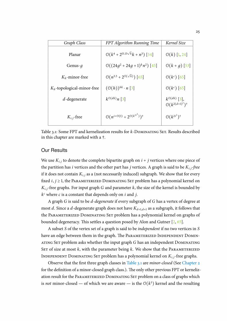
25
Graph Class FPT Algorithm Running Time Kernel Size
Planar O(k4 + 215.13√
kk + n3) [54] O(k) [1, 24]
Genus-д O((24д2 + 24д + 1)kn2) [45] O(k + д) [53]
Kh-minor-free O(n3.5 + 2O(
√
k)) [65] O(kc) [65]
Kh-topological-minor-free (O(h))hk ⋅ n [3] O(kc) [65]
d-degenerate kO(dk)n [3] kO(dk) [3],
O(k2(d+1)2
)†
Ki , j-free O(ni+O(1) + 2O(k2i2))† O(k2i
2
)†
Table 3.1: Some FPT and kernelization results for k-Dominating Set. Results described
in this chapter are marked with a †.
Our Results
We use Ki , j to denote the complete bipartite graph on i + j vertices where one piece of
the partition has i vertices and the other part has j vertices. A graph is said to be Ki , j-free
if it does not contain Ki , j as a (not necessarily induced) subgraph. We show that for every
xed i , j ≥ 1, the Parameterized Dominating Set problem has a polynomial kernel on
Ki , j-free graphs. For input graph G and parameter k, the size of the kernel is bounded by
kc where c is a constant that depends only on i and j.
A graph G is said to be d-degenerate if every subgraph of G has a vertex of degree at
most d. Since a d-degenerate graph does not have Kd+1,d+1 as a subgraph, it follows that
the Parameterized Dominating Set problem has a polynomial kernel on graphs of
bounded degeneracy.is settles a question posed by Alon and Gutner [2, 65].
A subset S of the vertex set of a graph is said to be independent if no two vertices in S
have an edge between them in the graph.e Parameterized Independent Domin-
ating Set problem asks whether the input graph G has an independent Dominating
Set of size at most k, with the parameter being k. We show that the Parameterized
Independent Dominating Set problem has a polynomial kernel on Ki , j-free graphs.
Observe that the rst three graph classes in Table 3.1 areminor-closed (See Chapter 2
for the denition of a minor-closed graph class.).e only other previous FPT or kerneliz-
ation result for the ParameterizedDominating Set problem on a class of graphs which
is not minor-closed — of which we are aware — is the O(k3) kernel and the resulting
26 CHAPTER 3. DOMINATION ON KI,J-FREE GRAPHS
FPT algorithm for graphs that exclude triangles and 4-cycles [102]. In fact, this result can
be modied to obtain similar bounds on graphs which have no 4-cycles, but may have
triangles. Since a 4-cycle is a K2,2, this latter result follows from the main result of the
current chapter by setting i = j = 2.
Since, for a constant h, a Kh-topological-minor-free graph has bounded degener-
acy [20, 65, 80], the class ofKi , j-free graphs ismore general than the class ofKh-topological-
minor-free graphs.us we extend the class of graphs for which the Parameterized
Dominating Set problem is known to have (1) FPT algorithms and (2) polynomial
kernels, to the class of Ki , j-free graphs. It is interesting to note that except for Ki , j-free
graphs, all the other graph classes in Table 3.1 are of bounded degeneracy, and are hence
sparse: any d-degenerate graph on n vertices has at most dn edges. In contrast, Ki , j-free
graphs can, in general, have a super-linear number of edges; for example, Alon et al. [5]
show that for suciently large i and for j > (i − 1)!, there exist Ki , j-free graphs on n
vertices with Ω(n2−1/i) edges.
Organization of the rest of the chapter
roughout this chapter, n denotes the number of vertices in the input graph. In Section 3.1
we present our main kernelization algorithm that, for xed j ≥ i ≥ 2, runs in O(ni) time
and constructs a kernel on O(( j + 1)i+1k i2
) vertices for Parameterized Dominating
Set on Ki , j-free graphs. As a corollary we obtain, in Section 3.2, a polynomial kernel
for the problem restricted to d-degenerate graphs, where the kernelization algorithm
runs in O(nd+1) time and outputs a kernel of size O((d + 2)d+3k(d+1)2). In Section 3.2.1
we describe an improvement to the above algorithm that applies to d-degenerate input
graphs, yields a kernel of the same size as above, and runs in timeO(2ddn2). In Section 3.3
we describe a modication of the algorithm in Section 3.1 that constructs a polynomial
kernel for the Parameterized Independent Dominating Set problem on Ki , j-free
graphs.is kernel has O( jk i) vertices, and so implies a kernel of size O((d + 1)2kd+1)
for this problem on d-degenerate graphs. In Section 3.4 we state our conclusions and list
some open problems.
Notation
All the graphs in this chapter are nite, undirected and simple. In general we follow the
graph terminology of Section 2.1. Let H be a graph obtained from a copy of a graph G by
applying some changes, and let S be a vertex subset of G whose copy survives in H. For
ease of presentation, we sometimes abuse notation and use S to denote the copy of S in
H as well.
3.1. A POLYNOMIAL KERNEL FOR KI,J-FREE GRAPHS 27
Note that we use the adjective “Ki , j-free” to denote graphs which do not contain
Ki , j as a subgraph. We would like to emphasize that this is dierent from the notion
of excluding Ki , j as an induced subgraph. A graph which excludes Ki , j as an induced
subgraphmay indeed contain Ki , j as a subgraph. We consider a simple example to buttress
this distinction. As noted below, the Parameterized Dominating Set problem has a
linear kernel on graphs which exclude K1,4 as a subgraph — that is, on K1,4-free graphs.
In stark contrast, the same problem is W[2]-hard on graphs which exclude K1,4 as an
induced subgraph [71].
3.1 A Polynomial Kernel for Ki , j-free Graphs
In this section we consider the Parameterized Dominating Set problem on graphs
that do not have Ki , j as a subgraph, for xed j ≥ i ≥ 1. If k = 1, then the problem can
be solved in linear time by checking if there is a vertex which is adjacent to all other
vertices in the graph. For i = 1, j ≥ i, a graph that does not have Ki , j as a subgraph has
degree at most j− 1. Any set of k vertices in such a graph G can dominate at most ( j− 1)k
other vertices, and so G is a Yes instance of Parameterized Dominating Set only if
G contains at most jk vertices.us the problem is (1) polynomial-time solvable when
k = 1, and (2) has a linear vertex kernel when i = 1, j ≥ i, and so in the rest of the chapter
we restrict our attention to the cases k > 1, j ≥ i ≥ 2.
We derive a polynomial kernel for a slightly more general, coloured version of the
Parameterized Dominating Set problem. We dene an rwb-graph (a red-white-blue
graph) to be a graph whose vertices are (arbitrarily) coloured with the three colours
red, white, and blue. More precisely, an rwb-graph is a graph G = (V , E) where V is
partitioned into RG ,WG , and BG (coloured red, white, and blue, respectively). An rwb-
dominating set of an rwb-graph G is a vertex subset S ⊆ V of G such that RG ⊆ S and
S dominates BG ; that is, it contains all red vertices and dominates all blue vertices. We
dene the Parameterized rwb-Dominating Set problem as follows:
Parameterized rwb-Dominating Set
Input: An rwb-graph G = (V , E) and a non-negative integer k.
Parameter: k
Question: Does G have an rwb-dominating set with at most k vertices?
e following simple claim shows that the coloured version of the problem is more
general.
28 CHAPTER 3. DOMINATION ON KI,J-FREE GRAPHS
Claim 1. Let G be a graph and H the rwb-graph obtained from G by colouring all the
vertices blue. en G has a dominating set of size at most k if and only if H has an rwb-
dominating set of size at most k.
Proof. Note that H is a copy of G with coloured vertices. Let S be a dominating set of
G of size at most k. Since the set RH of red vertices of H is empty, RH ⊆ S. Since H is
isomorphic to G as a graph, S dominates all vertices in H. Hence S is an rwb-dominating
set of H of size at most k.
Conversely, if S is an rwb-dominating set of H of size at most k, then since all vertices
in H are blue, S dominates all vertices in H. us S is a dominating set of G of size at
most k.
In our kernelization algorithm for Parameterized Dominating Set, we rst colour
all the vertices of the input graphG blue to obtain an rwb-graphH.en we apply certain
reduction rules toH. Roughly speaking, the reduction rules try to identify (1) vertices that
must necessarily be in every rwb-dominating set of H of size at most k, and (2) vertices
whose deletion from H does not aect the size of a minimal rwb-dominating set of H of
size at most k.
e reduction rules also colour various vertices red or white. Intuitively, the vertices
coloured red are those that will be picked up by the reduction rules in the rwb-dominating
set D of size at most k that we are trying to construct. In particular, if there is a k-
dominating set in the graph, the rules ensure that there will be one that contains all the
red vertices. Vertices which are known to have been already dominated by D are coloured
white. Clearly all neighbours of red vertices are white, but our reduction rules colour
some vertices white even if they have no red neighbours (at that point).ese are vertices
that will be dominated by one out of a small number of vertices identied by the reduction
rules: See reduction rule 2 for the details.e vertices that remain blue are those that are
yet to be dominated.
We rst describe an algorithm that takes as input an rwb-graph G on n vertices and a
positive number k, and runs in O(ni) time.e algorithm either nds that G does not
have any rwb-dominating set of size at most k, or it constructs an instance (H, k) on
O(( j + 1)i+1k i2
) vertices such that G has an rwb-dominating set of size at most k if and
only if H has an rwb-dominating set of size at most k. To complete the kernelization
procedure, we show that this instance (H, k) of Parameterized rwb-Dominating Set
can be converted into an equivalent instance of Parameterized Dominating Set—
that is, the colours can be removed — with a polynomially bounded increase in both the
number of vertices and the parameter value.
3.1. A POLYNOMIAL KERNEL FOR KI,J-FREE GRAPHS 29
e algorithm applies a sequence of reduction rules in a specied order.e input
and output of each reduction rule are rwb-graphs.
Denition 3.1. An rwb-graph G is said to be reduced with respect to a reduction rule ifan application of the rule to G does not change G.
e correctness of the kernelization algorithm depends on the fact that each reduction
rule satises the following correctness condition and preserves the invariants stated below:
Denition 3.2. (Correctness) A reduction rule R is said to be correct if the followingcondition holds: Let (G , k) be an instance of Parameterized rwb-Dominating Set,
and let (H, k′) be the instance of Parameterized rwb-Dominating Set obtained from
(G , k) by one application of rule R.en H has an rwb-dominating set D′ of size at most
k′ if and only if G has an rwb-dominating set D of size at most k.∗
We ensure that the following invariants are maintained aer every application of each
reduction rule.
Invariants:
1. None of the reduction rules introduces a Ki , j into a graph.
2. In the rwb-graphs constructed by the algorithm, no red vertex has a blue neighbour.
3. Let R1 and R2 be two reduction rules such that R1 precedes R2 in the order in
which the rules are presented below. Suppose (G1, k1) is reduced with respect to R1
and (G2, k2) is obtained by an application of rule R2 to (G1, k1).en (G2, k2) is
reduced with respect to R1.
3.1.1 The reduction rules and the kernelization algorithm
e kernelization algorithm assumes that the input graph is an rwb-graph. It applies the
following rules exhaustively in the given order. Each rule is repeatedly applied till it causes
no changes to the graph and then the next rule is applied.
We use some notational conventions in this section. For each rule below, (G , k)
denotes the instance on which the rule is applied, and (H, k′) the instance that is obtained
when the rule is applied to (G , k). Further, D,D′, k and k′ are as in Denition 3.2: D is
an rwb-dominating set of size k of G, and D′ an rwb-dominating set of H of size k′.
Our rst reduction rule is simple to state, and its correctness is almost self-evident:
∗ Note, however, that none of our reduction rules changes the value of k, and so k′ = k for every one of these
rules.
30 CHAPTER 3. DOMINATION ON KI,J-FREE GRAPHS
Rule 1. Let B be the set of all isolated blue vertices in G.
1. Colour all vertices in B red.
2. Set k′ ∶= k.
Lemma 3.1. Rule 1 is correct and preserves the invariants.
Proof. Let (G , k) be the instance on which the rule is applied, and (H, k) the resulting
instance. Let I be the set of isolated blue vertices in G.
Let D be an rwb-dominating set of G of size at most k. From the denition of an
rwb-dominating set, RG ⊆ D. Since an isolated vertex can only be dominated by itself,
I ⊆ D. Since the only thing that the rule does is to colour isolated blue vertices of G red,
RH = RG ∪ I, and so RH ⊆ D. Set D′ = D in H. en D′ dominates every vertex in H,
RH ⊆ D′, and ∣D′∣ ≤ k.us D′ is an rwb-dominating set of H of size at most k.
Conversely, let D′ be an rwb-dominating set of H of size at most k. Set D = D′ in
G. Since the only thing that the rule does is to colour isolated blue vertices of G red,
RG ⊆ RH ⊆ D′ = D, and so D is an rwb-dominating set of G of size at most k.us Rule 1
is correct.
e rule trivially preserves the rst two invariants, and vacuously preserves the third.
e next reduction rule is somewhat more involved, and may look mysterious at
rst. To motivate this rule, observe that if themaximum degree of a vertex in the input
graph is ∆, then any set of k vertices in the graph can dominate at most k∆ vertices, and
so the total number of vertices in a Yes instance is at most k(∆ + 1). is is precisely
the argument that we used at the beginning of this section to obtain a kernel on O( jk)
vertices for K1, j-free graphs. It is not clear, however, that this observation helps in any way
for bounding the size of Yes instances in Ki , j-free graphs when i ≥ 2. A K3,10-free graph,
for instance, can have a vertex of arbitrarily large degree, and the observation which relies
on a bounded maximum degree does not seem to be relevant in this case.
It turns out, in fact, that the bounded-degree argument does apply, but in a slightly
more involved manner, and aer a bit of preprocessing. To see how, consider again the
case of a K3,10-free graph G, which may contain vertices of arbitrarily large degree. Since a
bounded-degree argument does not directly apply toG, we look instead at pairs of vertices
which have a large common neighbourhood. So let u, v be two vertices which have more
than 10k common neighbours in G, and let B be this set of common neighbours. We
claim that if G has a dominating set of size at most k, then at least one of u, vmust be
present in every such dominating set.
3.1. A POLYNOMIAL KERNEL FOR KI,J-FREE GRAPHS 31
To see why, observe that no vertex w ∉ u, v has 10 or more neighbours in B, or
else the subgraph of G induced by the vertices u, v ,w and their common neighbours
contain a K3,10, a contradiction.us any vertex other than u, v can dominate at most
10 vertices which are in B; this maximum is attained when a vertex in B dominates 9
other vertices in B. Any set S of at most k vertices not intersecting u, v can therefore
dominate at most 10k vertices in B. Since B contains at least 10k + 1 vertices, S cannot
dominate all the vertices in B, and therefore cannot be a dominating set of G; the claim
follows.
For K3,10-free graphs we may thus have a reduction rule which says that if two vertices
u and v have a suciently large common neighbourhood, then we can colour all the
common neighbours of u and v white; this is because at least one of u, v is guaranteed to
be in any solution.is rule is, admittedly, somewhat weak compared to the bounded-
degree argument which we had for K1, j-free graphs. Further, it does not seem to cause
any progress: neither does it increase the number of vertices forced into the eventual
solution set, nor does it reduce the size of the instance. It turns out, however, that by
repeatedly applying this rule and its variants, we can in fact reduce the input instance to a
state where a bounded-degree argument applies. Our next reduction rule, which is in fact
a sequence of reduction rules, is motivated by these considerations:
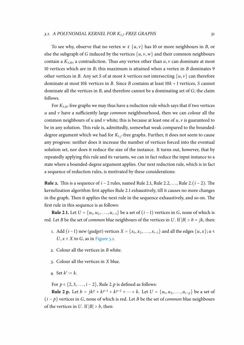
Rule 2. is is a sequence of i − 2 rules, named Rule 2.1, Rule 2.2, . . . , Rule 2.(i − 2).ekernelization algorithm rst applies Rule 2.1 exhaustively, till it causes no more changes
in the graph.en it applies the next rule in the sequence exhaustively, and so on.e
rst rule in this sequence is as follows:
Rule 2.1. Let U = u1, u2, . . . , ui−1 be a set of (i − 1) vertices in G, none of which is
red. Let B be the set of common blue neighbours of the vertices in U . If ∣B∣ > b = jk, then:
1. Add (i − 1) new (gadget) vertices X = x1, x2, . . . , xi−1 and all the edges u, x;u ∈
U , x ∈ X to G, as in Figure 3.1.
2. Colour all the vertices in B white.
3. Colour all the vertices in X blue.
4. Set k′ ∶= k.
For p ∈ 2, 3, . . . , i − 2, Rule 2.p is dened as follows:
Rule 2.p. Let b = jkp + kp−1 + kp−2 + ⋯ + k. Let U = u1, u2, . . . , ui−p be a set of
(i − p) vertices in G, none of which is red. Let B be the set of common blue neighbours
of the vertices in U . If ∣B∣ > b, then:
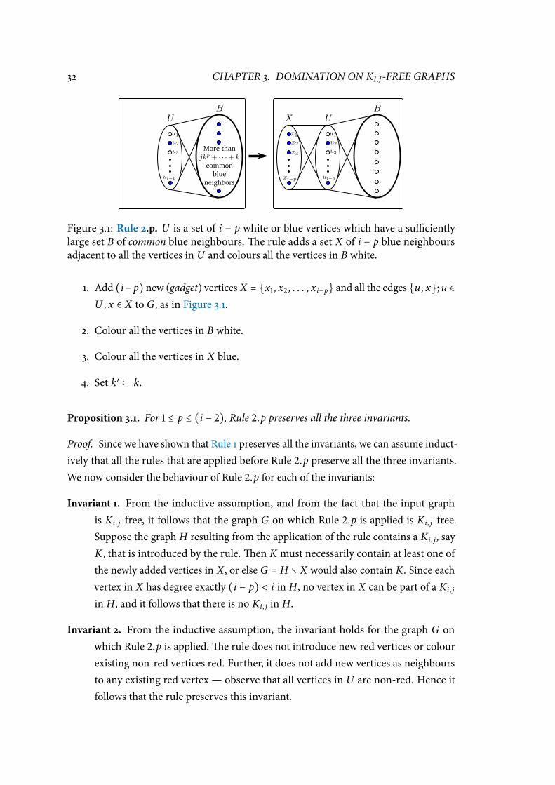
32 CHAPTER 3. DOMINATION ON KI,J-FREE GRAPHS
Figure 3.1: Rule 2.p. U is a set of i − p white or blue vertices which have a suciently
large set B of common blue neighbours.e rule adds a set X of i − p blue neighbours
adjacent to all the vertices in U and colours all the vertices in B white.
1. Add (i− p) new (gadget) vertices X = x1, x2, . . . , xi−p and all the edges u, x;u ∈
U , x ∈ X to G, as in Figure 3.1.
2. Colour all the vertices in B white.
3. Colour all the vertices in X blue.
4. Set k′ ∶= k.
Proposition 3.1. For 1 ≤ p ≤ (i − 2), Rule 2.p preserves all the three invariants.
Proof. Since we have shown that Rule 1 preserves all the invariants, we can assume induct-
ively that all the rules that are applied before Rule 2.p preserve all the three invariants.
We now consider the behaviour of Rule 2.p for each of the invariants:
Invariant 1. From the inductive assumption, and from the fact that the input graphis Ki , j-free, it follows that the graph G on which Rule 2.p is applied is Ki , j-free.
Suppose the graph H resulting from the application of the rule contains a Ki , j, say
K, that is introduced by the rule.en K must necessarily contain at least one of
the newly added vertices in X, or else G = H ∖ X would also contain K. Since each
vertex in X has degree exactly (i − p) < i in H, no vertex in X can be part of a Ki , j
in H, and it follows that there is no Ki , j in H.
Invariant 2. From the inductive assumption, the invariant holds for the graph G on
which Rule 2.p is applied.e rule does not introduce new red vertices or colour
existing non-red vertices red. Further, it does not add new vertices as neighbours
to any existing red vertex — observe that all vertices in U are non-red. Hence it
follows that the rule preserves this invariant.
3.1. A POLYNOMIAL KERNEL FOR KI,J-FREE GRAPHS 33
Invariant 3. Rule 2.1 preserves the invariant since it does not introduce isolated blue ver-tices into the graph. Assume inductively that for 2 ≤ p ≤ i−2, Rules 2.1, . . . , 2.(p−1)
preserve the invariant. So the graph G on which Rule 2.p is applied is reduced with
respect to Rules 1, 2.1, . . . , 2.(p − 1). Let H be the graph that results when Rule 2.p
is applied to G.en H is reduced with respect to Rule 1, since Rule 2.p does not
introduce isolated blue vertices in H.
Suppose H is not reduced with respect to Rule 2.q for some 1 ≤ q ≤ (p − 1).
en H contains a set U = u1, u2, . . . , ui−q of (i − q) non-red vertices such
that U has more than b common blue neighbours B, where b = jk if q = 1 and
b = jkq + kq−1 + kq−2⋯ + k otherwise. Either U or B (or both) must necessarily
contain at least one of the newly added vertices in X, or else G = H ∖ X would
also be not reduced with respect to Rule 2.q. Note that each vertex in X has degree
exactly (i − p) in H. Each vertex in U has degree at least b, and every vertex in B
has degree at least (i − q). Since p > q, we have (i − p) < (i − q). Since i ≤ j and
k ≥ 1, it follows that (i − p) < b. us no vertex in X can be part of either U or
B in H. It follows that H is reduced with respect to Rule 2.q, and hence Rule 2.p
preserves this invariant.
us the rule preserves all the three invariants.
Claim 2. Consider an application of Rule 2.p, 1 ≤ p ≤ i − 2. If U is a set of vertices of G
that satises the condition in Rule 2.p, then in every subset of V(G) of size at most k that
dominates B, there must be at least one vertex which is in U.
Proof. Let p = 1. Suppose there is a vertex set S ⊆ V(G) of size at most k such that (1) S
dominates B, and (2) S does not contain any vertex of U . Since ∣B∣ > jk, there is a vertex
v in S that dominates at least j + 1 vertices in B. Let T = N(v) ∩ B.en ∣T ∣ ≥ j, and the
vertex sets U ∪ v, T form the two parts of a Ki , j in G.is contradicts the Ki , j-free
property of the input graph or the rst invariant.
Now let 2 ≤ p ≤ (i − 2). Let S ⊆ V(G) be a set of size at most k that dominates B and
does not contain any vertex of U . Since ∣B∣ > b, there is a vertex v ∈ S that dominates at
least (b/k)+1 vertices in B. Because of the second invariant, v is not red. Let T = N(v)∩B.
en ∣T ∣ ≥ (b/k), and T is in the common neighbourhood of (U ∪ v).us (U ∪ v)
is a set of (i − (p − 1)) vertices in G, none of which is red, and which have at least
b/k > jkp−1 + kp−2 +⋯ + k common blue neighbours.is contradicts the fact that G is
reduced with respect to Rule 2.(p − 1).
We now argue that the gadget and the colouring correctly capture the structural
property guaranteed by Claim 2.
34 CHAPTER 3. DOMINATION ON KI,J-FREE GRAPHS
Proposition 3.2. Rule 2.p is correct for 1 ≤ p ≤ (i − 2).
Proof. Let D be an rwb-dominating set of G of size at most k, and let U be as in the
statement of Rule 2.p. Set D′ ∶= D. Since D is an rwb-dominating set of G, RG ⊆ D. Since
the rule does not add any new red vertices in H, it follows that RH ⊆ D′. Since (1) D
dominates all blue vertices of G, and (2) the rule removes no edges from G, it follows that
D′ = D dominates all blue vertices in H that are copies of blue vertices in G. By Claim 2,
D ∩ U ≠ ∅, and so D′ ∩ U ≠ ∅. Since all the new blue vertices added to H — namely,
those which constitute the set X — are adjacent to every vertex in U by construction, D′
dominates all blue vertices in H.us D′ is an rwb-dominating set of H of size at most k.
Conversely, let D′ be an rwb-dominating set of H of size at most k. We consider three
cases:
D′ ∩U = ∅. In this case, since D′ dominates X and X is an independent set, X ⊆ D′. Set
D ∶= (D′∖X)∪U . Since X andU are disjoint sets of equal cardinality, ∣D∣ ≤ ∣D′∣ ≤ k.
Since D′ is an rwb-dominating set of H, RH ⊆ D′. Since all vertices in X are blue
and since the reduction rule does not delete any red vertex from G to obtain H, it
follows that RG ⊆ D. Now, all the blue vertices dominated by X in H are contained
in U and U ⊆ D. Further, the set of vertices which are blue in G and white in H
is exactly the set B, and each vertex in U dominates all vertices in B.erefore D
dominates all blue vertices in G, and thus D is an rwb-dominating set of G of size
at most k.
D′ ∩ X = ∅. In this case, since D′ dominates X, it follows that D′ ∩U ≠ ∅. Set D ∶= D′.
en ∣D∣ = ∣D′∣ ≤ k. For the same reasons as above, RG ⊆ D, and D dominates all
vertices (namely, the set B) which are blue inG and white inH. Since D′ dominates
all blue vertices inH, and sinceG can be obtained fromH by deleting a set (namely,
X) of blue vertices and making the set B of white vertices blue, D = D′ dominates
all blue vertices in G.us D is an rwb-dominating set of G of size at most k.
D′ ∩U ≠ ∅,D′ ∩ X ≠ ∅. In this case, pick an arbitrary vertex v ∈ B and set D ∶= (D′ ∖
X) ∪ v. Since D′ ∩ X ≠ ∅, it follows that ∣D∣ ≤ ∣D′∣ ≤ k. For the same reasons
as above, RG ⊆ D, and D dominates all vertices (namely, the set B) which are blue
in G and white in H. Since D′ dominates all blue vertices in H, D′ ∖ X dominates
all blue vertices in H ∖ X, except possibly for some blue vertices in U whose only
neighbours in D′ belong to X. But the vertex v dominates all vertices in U , and so
D is an rwb-dominating set of G of size at most k.
ese three cases are exhaustive, and so it follows that for 1 ≤ p ≤ (i − 2), Rule 2.p is
correct.
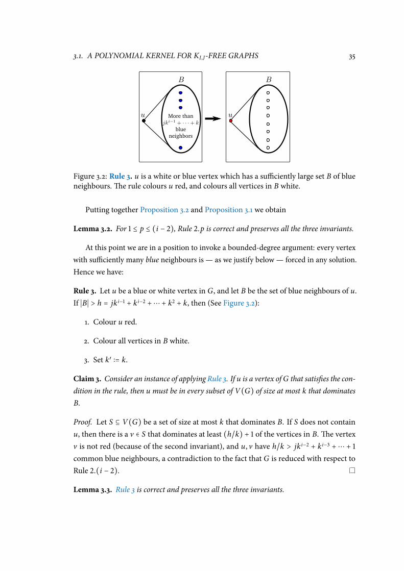
3.1. A POLYNOMIAL KERNEL FOR KI,J-FREE GRAPHS 35
Figure 3.2: Rule 3. u is a white or blue vertex which has a suciently large set B of blueneighbours.e rule colours u red, and colours all vertices in B white.
Putting together Proposition 3.2 and Proposition 3.1 we obtain
Lemma 3.2. For 1 ≤ p ≤ (i − 2), Rule 2.p is correct and preserves all the three invariants.
At this point we are in a position to invoke a bounded-degree argument: every vertex
with suciently many blue neighbours is — as we justify below — forced in any solution.
Hence we have:
Rule 3. Let u be a blue or white vertex in G, and let B be the set of blue neighbours of u.If ∣B∣ > h = jk i−1 + k i−2 +⋯ + k2 + k, then (See Figure 3.2):
1. Colour u red.
2. Colour all vertices in B white.
3. Set k′ ∶= k.
Claim 3. Consider an instance of applying Rule 3. If u is a vertex of G that satises the con-
dition in the rule, then u must be in every subset of V(G) of size at most k that dominates
B.
Proof. Let S ⊆ V(G) be a set of size at most k that dominates B. If S does not contain
u, then there is a v ∈ S that dominates at least (h/k) + 1 of the vertices in B.e vertex
v is not red (because of the second invariant), and u, v have h/k > jk i−2 + k i−3 + ⋯ + 1
common blue neighbours, a contradiction to the fact that G is reduced with respect to
Rule 2.(i − 2).
Lemma 3.3. Rule 3 is correct and preserves all the three invariants.

36 CHAPTER 3. DOMINATION ON KI,J-FREE GRAPHS
Proof. Let D be an rwb-dominating set of G of size at most k, and let u be as in the
statement of Rule 3. Set D′ ∶= D. Since D is an rwb-dominating set of G, RG ⊆ D. From
Claim 3, u ∈ D.e rule does not add any new vertex toG to obtain H. Since u is the only
vertex that is red in H and not red in G, RH = (RG ∪ u) ⊆ D′. Since (1) D dominates all
blue vertices of G, (2) the rule does not add new blue vertices or make non-blue vertices
blue, and (3) the rule removes no edges from the graph, it follows that D′ = D dominates
all blue vertices in H.us D′ is an rwb-dominating set of H of size at most k.
Conversely, let D′ be an rwb-dominating set of H of size at most k. en from
Claim 3, u ∈ D′. Set D ∶= D′. Since D′ is an rwb-dominating set of H, RH ⊆ D′. Since
RG = RH ∖ u, RG ⊆ D. Since (1) D′ dominates all blue vertices in H, (2) the only blue
vertices in G that are not blue in H are in B ∪ u, and (3) u ∈ D dominates B ∪ u, it
follows that D = D′ dominates all blue vertices in G.us D is an rwb-dominating set of
G of size at most k.
As for the invariants, Rule 3 does not change the structure of the graph. Further, it
gives the colour white to all blue neighbours of the only vertex — namely, u—whose
colour it changes to red. It follows that Rule 3 preserves all the three invariants.
Recall that we started the reduction from an rwb-graph which had no white vertices,
and we ensured that every reduction rule is correct. It follows from our notion of cor-
rectness (See Denition 3.2) that if the current rwb-graph G has an rwb-dominating
set of size at most k, then all vertices which are coloured white in G are guaranteed to
be dominated by some rwb-dominating set D of G of size at most k.is opens up the
possibility that we may be able to deduce that some white vertices are not required in
some solution, essentially since every blue vertex that they dominate is also dominated by
some other vertices in the solution.e next two reduction rules remove white vertices
which are dispensable, in the sense that there exists a solution which does not contain
these vertices.
It is intuitively clear that a white vertex that has no blue neighbour is dispensable. It is
also true that a white vertex which has just one blue neighbour is dispensable as well; the
intuition is that we might instead pick into any solution the one blue neighbour, with no
loss of generality.is motivates our next reduction rule:
Rule 4. If a white vertex u is adjacent to at most one blue vertex in G, then
1. Delete u from G,
2. Set k′ ∶= k, and
3. Apply Rule 1.

3.1. A POLYNOMIAL KERNEL FOR KI,J-FREE GRAPHS 37
Lemma 3.4. Rule 4 is correct and preserves all the three invariants.
Proof. Since we have already proved that Rule 1 is correct and preserves the three invari-
ants, it suces to show that the rst two steps of Rule 4 have the stated properties∗. We
now proceed to do this; in the following, whenever we refer to Rule 4, we mean the rst
two steps of this rule.
Let D be an rwb-dominating set of G of size at most k, and let u be as in the statement
of Rule 4. We consider two cases:
u ∉ D. In this case, set D′ ∶= D. Since D is an rwb-dominating set of G, and since
the rule only deletes a white vertex u ∉ D to obtain H, it follows that D′ is an
rwb-dominating set of H of size at most k.
u ∈ D. In this case, let A = (N(u) ∩ BG) be the set of blue neighbours of u in G. Note
that ∣A∣ ≤ 1. Set D′ ∶= (D ∖ u) ∪ A. Since ∣A∣ ≤ 1, ∣D′∣ ≤ ∣D∣ ≤ k. Since D is an
rwb-dominating set of G, RG ⊆ D. Since the rule only deletes a white vertex u to
obtain H, it follows that RH = RG ⊆ D′. Since (1) D dominates all blue vertices of G,
(2) D′ contains A, the set of all blue vertices of G dominated by the vertex u that
the rule deletes, and (3) the rule removes no edges from the graph other than those
adjacent to the removed white vertex u, it follows that D′ = D dominates all blue
vertices in H.us D′ is an rwb-dominating set of H of size at most k.
Conversely, let D′ be an rwb-dominating set of H of size at most k. Set D ∶= D′. Since
D′ is an rwb-dominating set of H, and since G can be obtained from H by adding a white
vertex u and some edges incident on u to H, D = D′ is an rwb-dominating set of G of
size at most k.
As for the invariants, since Rule 4 only deletes a vertex, its application cannot introduce
any of the subgraphs that make it possible to apply Rule 2 or Rule 3 to H. It is possible
that new isolated blue vertices may be introduced in H, but then the application of Rule 1
ensures that such vertices do not survive once Rule 4 is completely applied. It follows that
Rule 4 preserves all the three invariants.
At this stage each white vertex has at least two blue neighbours. If two white vertices
u, v have the same set of blue vertices as their respective neighbourhoods, then it is intuit-
ively clear that one of these white vertices — say u— is dispensable in the sense described
earlier: we can, without loss of generality, replace u with v in any rwb-dominating set.
is intuition is formalized below, and justies our next reduction rule:
∗ Except for arguing that the rule preserves the invariants: see below.

38 CHAPTER 3. DOMINATION ON KI,J-FREE GRAPHS
Figure 3.3: Rule 5. u is a white vertex whose set of blue neighbours is identical to the blueneighbourhood of a white or blue vertex v.e rule deletes u.
Rule 5. Let u be a white vertex in G, and let v be a white or blue vertex. If these twovertices have identical sets of blue neighbours — that is, if N[u]∩BG = N[v]∩BG — then
(See Figure 3.3):
1. Delete u from G
2. Set k′ ∶= k
Lemma 3.5. Rule 5 is correct and preserves all the three invariants.
Proof. Let D be an rwb-dominating set of G of size at most k, and let u, v be as in the
statement of Rule 5. We consider two cases:
u ∉ D. In this case, set D′ ∶= D. Since D is an rwb-dominating set of G, and since
the rule only deletes a white vertex u ∉ D to obtain H, it follows that D′ is an
rwb-dominating set of H of size at most k.
u ∈ D. In this case, set D′ ∶= (D ∖ u) ∪ v. en ∣D′∣ = ∣D∣ ≤ k. Since D is an rwb-
dominating set of G, RG ⊆ D. Since the rule only deletes a white vertex u to obtain
H, it follows that RH = RG ⊆ D′. Since (1) D dominates all blue vertices of G, (2) D′
contains a vertex — namely, v — that dominates all blue vertices dominated by the
vertex u that the rule deletes, and (3) the rule removes no edges from the graph
other than those adjacent to the removed white vertex u, it follows that D′ = D
dominates all blue vertices in H.us D′ is an rwb-dominating set of H of size at
most k.
Conversely, let D′ be an rwb-dominating set of H of size at most k. Set D ∶= D′. Since
D′ is an rwb-dominating set of H, and since G can be obtained from H by adding a white
vertex u and some edges incident on u to H, D = D′ is an rwb-dominating set of G of
size at most k.

3.1. A POLYNOMIAL KERNEL FOR KI,J-FREE GRAPHS 39
Since Rule 5 only deletes a vertex, its application cannot introduce any of the subgraphs
that make it possible to apply Rule 2, Rule 3, or Rule 4 to H. No new isolated blue vertex
is introduced in H, since u is the only deleted vertex, and all blue neighbours of u have at
least one other neighbour that survives in H, namely the vertex v. It follows that Rule 5
preserves all the three invariants.
If there are too many red or blue vertices, then we can conclude that the input is a No
instance:
Rule 6. If the graph G contains more than k red vertices or more than jk i + k i−1 + k i−2 +
⋯ + k2 blue vertices, then set (H, k′) to be a trivial No-instance of the problem; for
instance, make H the independent set on two blue vertices and set k′ = 1. If neither of
these conditions hold, set H ∶= G , k′ ∶= k.
Lemma 3.6. Rule 6 is correct and preserves all the three invariants.
Proof. Note that if the instance (G , k) satises neither of the two conditions, then the rule
returns the instance unchanged.erefore, to show that the rule is correct, it is sucient
to show that an instance (G , k) that satises either of the two conditions is a No-instance.
If ∣RG ∣ > k, then since every rwb-dominating set of G must contain all of RG , G has
no rwb-dominating set of size at most k.
From the second invariant, no blue vertex ofG has a red neighbour. SinceG is reduced
with respect to Rule 1 to Rule 5, nowhite or blue vertex inG hasmore than jk i−1+k i−2+⋯+k
blue neighbours, or else Rule 3 would have applied, contradicting the third invariant. So
k white or blue vertices in G can dominate at most jk i + k i−1 + k i−2 +⋯+ k2 blue vertices.
Hence if ∣BG ∣ > jk i + k i−1 + k i−2 +⋯ + k2, then no set of k vertices in G can dominate all
of BG , and so in this case G has no rwb-dominating set of size at most k.
e reduction rule either returns the instance unchanged or returns a simple No-
instance. In both cases, it trivially satises all the three invariants.
3.1.2 Algorithm correctness, running time, and kernel size
Recall that the input to the kernelization algorithm is a pair (G , k) where G is an rwb-
graph and k is a non-negative integer.e algorithm applies Rule 1 to Rule 6, in this order,
to (G , k), exhaustively applying each rule before applying the next. From the correctness
of Rule 1 to Rule 6 — see Lemma 3.1 to Lemma 3.6 — we obtain
Lemma 3.7. e kernelization algorithm is correct: Let (G , k) be the input to the al-
gorithm. If the algorithm says No, then G does not have an rwb-dominating set of size
at most k. Otherwise, let H be the rwb-graph output by the algorithm. en G has an
40 CHAPTER 3. DOMINATION ON KI,J-FREE GRAPHS
rwb-dominating set of size at most k if and only if H has an rwb-dominating set of size at
most k.
We now show that the kernelization algorithm runs in polynomial time. To do so, we
rst show that the algorithm does not add too many gadget vertices to the input graph.
Claim 4. Let (G , k) be the input to the kernelization algorithm, where G is a Ki , j-free
rwb-graph on n vertices.e total number of gadget vertices that the algorithm adds to the
graph, over all applications of rules 2.1 to 2.(i − 2), is less than n.
Proof. We reuse the notation used to describe rules 2.1 to 2.(i − 2). Rule 2.1 colours all
vertices in B white, and adds the new all-blue gadget vertex set X to the graph.e set
B contains at least ( jk + 1) blue vertices, and the set X has exactly (i − 1) blue vertices.
us one application of Rule 2.1 reduces the count of blue vertices in the graph by at least
( jk − i + 2). By a similar argument, we can see that for 2 ≤ p ≤ i − 2, each application of
Rule 2.p reduces the count of blue vertices by at least ( jkp + kp−1+⋯+ k− i + p+ 1). Since,
by assumption, j ≥ i ≥ 2 and k ≥ 2, it follows that ( jk− i+2) ≤ ( jkp+kp−1+⋯+k− i+p+1)
for 2 ≤ p ≤ i − 2. us each application of one of the rules 2.1 to 2.(i − 2) reduces the
total number of blue vertices in the graph by at least ( jk − i + 2). Also, observe that the
number of gadget vertices added to the graph in each application of one of the rules 2.1
to 2.(i − 2) is at most (i − 1), where this maximum is attained for Rule 2.1.
Consider an application of Rule 2.p for some 1 ≤ p ≤ i − 2. A blue or white vertex can
be part of a set U as mentioned in the rule only if it has at least jkp + kp−1 + kp−2 +⋯ + k
blue neighbours. Since the maximum number of blue neighbours that a gadget vertex can
have is i− 1, it follows that no gadget vertex will ever be part of the setU in any application
of Rule 2.p. Since the rwb-graph given as input to the kernelization algorithm has exactly
n blue vertices, rules 2.1 to 2.(i − 2) can thus be applied at most n/( jk − i + 2) times in
total, over the full course of the algorithm. So the total number of gadget vertices added
to the graph over all applications of rules 2.1 to 2.(i − 2) is n(i − 1)/( jk + 2 − i), and this
number is less than n since we assume that k is at least 2.
is bound on the number of gadget vertices helps in showing that the algorithm
runs in polynomial time.
Lemma 3.8. e kernelization algorithm can be implemented in such a way as to run in
O (max(n2, ini)) time when the input instance is a Ki , j-free rwb-graph G on n vertices
and m edges.
Proof. We assume that the input rwb-graph is given in the form of a modied adjacency
list.is representation diers from the standard adjacency list representation in two
ways:
3.1. A POLYNOMIAL KERNEL FOR KI,J-FREE GRAPHS 41
1. ere is a provision for colouring each vertex red, white, or blue.
2. Let u, v be two vertices such that u, v is an edge in the graph. Let vu be the node
for v in the adjacency list of u, and uv the node for u in the adjacency list of v.en
vu contains a pointer to uv , and uv contains a pointer to vu.
is is not a costly assumption: Observe that we can add a new vertex x to such amodied
adjacency list L in time linear in the number of edges from x to the vertices which are
already present in L. It follows that one can convert an adjacency matrix or adjacency list
representation of the input rwb-graph to the modied form in time linear in the size of
the original representation.
Observe that Claim 4 implies that the total number of vertices in the graph at any
point during the execution of the algorithm does not exceed 2n. We now analyze the time
taken to exhaustively apply each rule.
Rule 1, Rule 3 Each application of one of these two rules colours at least one blue vertexred. No reduction rule changes the colour of a red vertex. From the bound on the
total number of vertices in the graph, it follows that Rule 1 and Rule 3 can be applied
at most 2n times each. One application of each of these two rules can be done in
O(n) time by a constant number of scans of the vertex list in the input graph, and
so both these rules can be applied exhaustively in O(n2) time.
Rule 2 As argued in the proof of Claim 4, no gadget vertex need ever be considered forinclusion in the set U in any application of Rule 2.p. For applying Rule 2.p for a
xed 1 ≤ p ≤ i − 2, therefore, the algorithm iterates over all (i − p)-subsets of the set
of all original (not gadget) vertices which are blue or white (at this point).is can
be done in O((n
i−p)) time, as was rst shown by Ehrlich [44]. For each such subset
S, the algorithm nds the set of common blue neighbours of S as in Algorithm 1.
Since the total number of possible blue vertices — including gadget vertices — is at
most 2n (see Claim 4), this can be done in time O((i − p)n). A straightforward
implementation of the remaining part of Rule 2.p runs in O(n + (i − p)2) = O(n)
time (since i − p = O(1)), and so Rule 2.p can be exhaustively applied in (n
i−p) ⋅
(O((i − p)n) + O(n)) = ni−p
(n−1
i−p−1) ⋅ O((i − p)n) = O(ni−p+1) time. All the rules
2.p; 1 ≤ p ≤ i − 2 can therefore be exhaustively applied in O(ini) time.
Rule 4 Each application of this rule deletes at least one white vertex. From the boundon the total number of vertices in the graph, it follows that the rule can be applied
at most 2n times. Each application of the rule essentially consists of the deletion
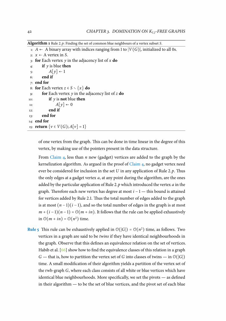
42 CHAPTER 3. DOMINATION ON KI,J-FREE GRAPHS
Algorithm 1 Rule 2.p: Finding the set of common blue neighbours of a vertex subset S.1: A← A binary array with indices ranging from 1 to ∣V(G)∣, initialized to all 0s.
2: x ← A vertex in S.
3: for Each vertex y in the adjacency list of x do4: if y is blue then5: A[y]← 1
6: end if7: end for8: for Each vertex z ∈ S ∖ x do9: for Each vertex y in the adjacency list of z do10: if y is not blue then11: A[y]← 0
12: end if13: end for14: end for15: return v ∈ V(G);A[v] = 1
of one vertex from the graph.is can be done in time linear in the degree of this
vertex, by making use of the pointers present in the data structure.
From Claim 4, less than n new (gadget) vertices are added to the graph by the
kernelization algorithm. As argued in the proof of Claim 4, no gadget vertex need
ever be considered for inclusion in the set U in any application of Rule 2.p.us
the only edges at a gadget vertex a, at any point during the algorithm, are the ones
added by the particular application of Rule 2.p which introduced the vertex a in the
graph.erefore each new vertex has degree at most i − 1 — this bound is attained
for vertices added by Rule 2.1.us the total number of edges added to the graph
is at most (n − 1)(i − 1), and so the total number of edges in the graph is at most
m + (i − 1)(n − 1) = O(m + in). It follows that the rule can be applied exhaustively
in O(m + in) = O(n2) time.
Rule 5 is rule can be exhaustively applied in O(∣G∣) = O(n2) time, as follows. Two
vertices in a graph are said to be twins if they have identical neighbourhoods in
the graph. Observe that this denes an equivalence relation on the set of vertices.
Habib et al. [66] show how to nd the equivalence classes of this relation in a graph
G — that is, how to partition the vertex set of G into classes of twins — in O(∣G∣)
time. A small modication of their algorithm yields a partition of the vertex set of
the rwb-graph G, where each class consists of all white or blue vertices which have
identical blue neighbourhoods. More specically, we set the pivots — as dened
in their algorithm — to be the set of blue vertices, and the pivot set of each blue

3.1. A POLYNOMIAL KERNEL FOR KI,J-FREE GRAPHS 43
vertex to be its closed neighbourhood. It is straightforward to verify that with this
modication, their algorithm yields a partition of V(G) of the desired kind in
O(∣G∣) time. We now go through each equivalence class, and if a class contains
a white vertex u and at least one other vertex, then we delete u. By making use
of the pointers present in the data structure that represents the graph G, all these
deletions can be eected in O(∣G∣) time.
Putting all these together, the kernelization algorithm can be implemented to run in
O (max(n2, ini)) time.
Now we prove a polynomial bound on the size of the reduced instance.
Lemma3.9. Let (G , k) be the input to the kernelization algorithm. If the algorithm outputs
the instance (H, k), then ∣V(H)∣ = O(( j + 1)i+1k i2
).
Proof. From Rule 6, we get ∣RH ∣ ≤ k and b = ∣BH ∣ ≤ jk i + k i−1 +⋯+ k ≤ ( j+ 1)k i . Now we
bound ∣WH ∣. Note that no two white vertices inH can have identical blue neighbourhoods,
or else Rule 5 would have applied. Also, each white vertex has at least two blue neighbours,
or else Rule 4 would have applied. Hence the number of white vertices in H that have
less than i blue neighbours is at most (b2) + (
b
3) + ⋯ + (
b
i−1) ≤ 2b i−1. No set of i blue
vertices in H has more than ( j − 1) common white neighbours, or else these form a Ki , j.
Hence the number of white vertices that have i or more blue neighbours in H is at most
(b
i)( j − 1) ≤ ( j − 1)b i . So the total number of white vertices in H,
∣WH ∣ ≤ 2bi−1 + ( j − 1)b i
= (2 + ( j − 1)b)b i−1
≤ ( j + 1)b i
≤ ( j + 1)(( j + 1)k i)i
= ( j + 1)i+1k i2
e bound in the lemma follows.
From Lemma 3.8 Lemma 3.9 we obtain
Corollary 3.1. For every xed j ≥ i ≥ 1, the Parameterized rwb-Dominating Set
problem on Ki , j-free graphs has a polynomial kernel with O(( j + 1)i+1k i2
) vertices.
44 CHAPTER 3. DOMINATION ON KI,J-FREE GRAPHS
3.1.3 Removing the colours
ByClaim 1, the Parameterized rwb-Dominating Set problem is amore general version
of the Parameterized Dominating Set problem. By Corollary 3.1, Parameterized
rwb-Dominating Set has a polynomial kernel on Ki , j-free graphs, and therefore, intu-
itively, so should Parameterized Dominating Set. is intuition is in fact justied,
because the notion of Parameterized rwb-Dominating Set being “more general” than
Parameterized Dominating Set captures the fact that there is a “nice” polynomial-
timemany-to-one reduction from ParameterizedDominating Set to Parameterized
rwb-Dominating Set. To be more precise:
• By Claim 1, Parameterized Dominating Set polynomial-time reduces to Para-
meterized rwb-Dominating Set, and the reduction preserves the parameter— k
goes to k.
• Parameterized rwb-Dominating Set is inNP—a solution by itself is a certicate
which is veriable in polynomial time.
• Parameterized Dominating Set is NP-hard in Ki , j-free graphs, since it is NP-
hard in K2,2-free graphs; see, for example, the reduction from the 3-SAT problem
attributed to David Johnson [69,eorem 1.7].
erefore, to obtain a polynomial kernel for Parameterized Dominating Set in
Ki , j-free graphs, one can do the following:
• Use Claim 1 to reduce Parameterized Dominating Set to Parameterized
rwb-Dominating Set in polynomial time, preserving the parameter.
• Use Corollary 3.1 to obtain a polynomial kernel for the Parameterized rwb-
Dominating Set instance obtained in the previous step.
• Apply the polynomial-time many-to-one reduction from Parameterized rwb-
Dominating Set to Parameterized Dominating Set in Ki , j-free graphs, to the
Parameterized rwb-Dominating Set kernel obtained in the above step.
Since the Parameterized rwb-Dominating Set kernel is of polynomial size in the
original parameter k, and the last reduction runs in polynomial time, the resulting
Parameterized Dominating Set instance has size, and hence parameter, polynomial
in k. is argument shows that Parameterized Dominating Set has a polynomial
kernel when restricted to Ki , j-free graphs, but does not give an explicit bound on the
kernel size. We now describe a specic polynomial-time many-to-one reduction from

3.1. A POLYNOMIAL KERNEL FOR KI,J-FREE GRAPHS 45
Figure 3.4: Removing the colours. W1 is the set of white vertices which are adjacent to
red vertices, andW2 are the other white vertices.e rule attaches a pendant to each red
vertex, a pendant path of length two to each vertex inW2, and removes all the colours.
Parameterized rwb-Dominating Set to ParameterizedDominating Set inKi , j-free
graphs and derive a concrete upper bound on the size of the kernel.
Let (G , k) be an instance of the Parameterized Dominating Set problem on
Ki , j-free graphs. To obtain a polynomial kernel for this instance, we rst colour all
the vertices of G blue to obtain an equivalent instance of the Parameterized rwb-
Dominating Set problem.en we apply Corollary 3.1 on this Parameterized rwb-
Dominating Set instance to obtain a reduced instance (G′, k) of the problem, where
∣V(G′)∣ = O(( j + 1)i+1k i2
).
We then apply the following steps (See Figure 3.4) to transform the reduced coloured
instance (G′, k) to an instance (H, k+w) of (uncoloured) ParameterizedDominating
Set, where w = O(( j + 1)i+1k i2
) is the number of white vertices in G′ which have no red
neighbours.is involves a signicant increase in the value of the parameter, which is
somewhat unusual: for most known kernels the new parameter is upper bounded by the
original value of the parameter, or by a constant additive or multiplicative factor of the
original value.
1. For each white vertex u that has no red neighbour, add two new vertices u1, u2 and
the edges u, u1, u1, u2.at is, create a new path with two edges starting at u.
LetM be the set of all “middle” vertices u1 added in this manner.
2. For each red vertex v, add a new vertex v1 and the edge v , v1.at is, add a new
pendant vertex attached to v.
3. Remove all colours from the vertices.
Note that this construction does not introduce a Ki , j into the graph, and that it increases
the number of vertices in the graph by at most a factor of 3. We use the extra vertices
46 CHAPTER 3. DOMINATION ON KI,J-FREE GRAPHS
to encode the information which is captured by colours in the coloured instance. More
precisely, suppose G′ has an rwb-dominating set S of size at most k. By denition, the
vertex set S contains all the red vertices and dominates all the blue vertices inG′.erefore,
in the graph H the same set S dominates the following sets of vertices: (1) all vertices
which were red inG′, and all their neighbours, including all the pendant vertices added in
Step 2 above, and, (2) all the vertices which were blue in G′.e only vertices in H which
are not dominated by S are: (1) those white vertices in G′ which had no red neighbours,
and (2) the new vertices added to G′ by Step 1 of the above construction.e set M of
“middle” vertices added in Step 1 above dominates all these vertices in H, and so S ∪M is
a dominating set of H of size at most k +w.
Conversely, suppose H has a dominating set of size at most k +w, and let X be an
inclusion-minimal dominating set of H of size at most k +w.en we may assume the
following about X without loss of generality:
1. X contains all the vertices which were red in G′: RG′ ⊆ X,
2. X contains all the “middle” vertices added in Step 1: M ⊆ X, and,
3. X does not contain any pendant vertex added in Step 1 or Step 2.
To see these, observe rst that if X does not contain a vertex v which was red in G′,
then it must contain the pendant vertex v1 added in Step 2 of the construction, because
X must dominate v1. e set (X ∖ v1) ∪ v is then a dominating set of H of the
same size as X which contains one more vertex which was red in G′, which justies the
rst assumption. A similar argument using the pendant vertices added in Step 1 of the
construction shows that we may assume that X contains all the “middle” vertices added
in this step. Finally, if v1 ∈ X is a pendant vertex added in Step 1 or Step 2, then since X
contains — by the rst two assumptions — a vertex v adjacent to v′, the set X ∖ v′ is a
smaller dominating set of H, and this contradicts the minimality of X.
Now observe that the vertices inM do not dominate any vertex which was blue in G′.
Since (1) (RG′ ∪M) ⊆ X, (2) the set X does not contain any pendant vertex added by the
construction, and (3) ∣M∣ = w, it follows that X∖M is a set of atmost k vertices inG′ which
contains all the red vertices and dominates all the blue vertices.us the above reduction
from Parameterized rwb-Dominating Set to Parameterized Dominating Set is
sound, and so from Corollary 3.1 we have
eorem 3.1. For every xed j ≥ i ≥ 1, the Parameterized Dominating Set problem on
Ki , j-free graphs has a polynomial kernel with O(( j + 1)i+1k i2
) vertices.
3.2. A POLYNOMIAL KERNEL FOR D-DEGENERATE GRAPHS 47
3.2 A Polynomial Kernel for d-degenerate Graphs
A d-degenerate graph does not contain Kd+1,d+1 as a subgraph, and so the kernelization
algorithm of the previous section can be applied to a d-degenerate graph, setting i =
j = d + 1.e algorithm runs in O(max(n2, (d + 1)nd+1)) time and constructs a kernel
with O((d + 2)d+2 ⋅ k(d+1)2) vertices. Since a d-degenerate graph on v vertices has at most
dv edges, we have:
Corollary 3.2. e Parameterized Dominating Set problem on d-degenerate graphs
has a kernel on O((d + 2)d+3 ⋅ k(d+1)2) vertices and edges.
Corollary 3.2 settles an open problem posed by Alon and Gutner [2, 65].
3.2.1 Improving the running time
We describe a modication to our algorithm that reduces the running time toO(2d ⋅d ⋅n2)
when the input is restricted to d-degenerate graphs; the bound on the kernel size remains
the same.e modied algorithm makes use of the following well-known property of
d-degenerate graphs:
Fact 1. [57, eorem 2.10] Let G be a d-degenerate graph on n vertices. en one can
compute, in O(dn) time, an ordering v1, v2, . . . , vn of the vertices of G such that for 1 ≤ i ≤
n, vi has at most d neighbours in the subgraph of G induced on vi , . . . , vn.
e modication to the algorithm pertains to the way in which rules 2.1 to 2.(d − 1)
are implemented: the rest of the algorithm remains the same.
e previous implementation of Rule 2.p, 1 ≤ p ≤ (d−1), checks each (d−p+1)-subset
of vertices in the graph to see if it satises the condition in the rule. When the graph is
degenerate, we instead make use of Fact 1 to quickly nd such a set of vertices, if it exists.
Let G be the graph instance on n vertices on which Rule 2.p is to be applied. First we
delete, temporarily, all the red vertices in G. We then nd an ordering v1, v2, . . . , vn of the
kind described in Fact 1, of all the remaining vertices in G. Let U and B be as dened in
the rule. Since each vertex in U has degree greater than d, the rst vertex vl in U ∪ B that
appears in the ordering has to be from B.e vertex vl will then have a neighbourhood
of size d − p+ 1 that in turn has B as its common neighbourhood. We use this fact to look
for such a pair (U , B) and exhaustively apply Rule 2.p to G; see Algorithm 2. We then
add back the red vertices that we deleted prior to this step, along with all their edges to
the rest of the graph.
As ∣N ∣ ≤ d, the inner for loop is executed at most ( d
p−1) times for each iteration of the
outer loop. Each of the individual steps in the algorithm can be done in O(dn) time, and
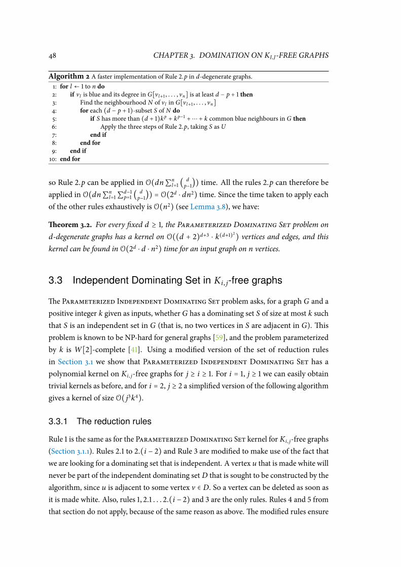
48 CHAPTER 3. DOMINATION ON KI,J-FREE GRAPHS
Algorithm 2 A faster implementation of Rule 2.p in d-degenerate graphs.1: for l ← 1 to n do2: if v l is blue and its degree in G[v l+1 , . . . , vn] is at least d − p + 1 then3: Find the neighbourhood N of v l in G[v l+1 , . . . , vn]
4: for each (d − p + 1)-subset S of N do5: if S has more than (d + 1)kp
+ kp−1+⋯ + k common blue neighbours in G then
6: Apply the three steps of Rule 2.p, taking S as U
7: end if8: end for9: end if10: end for
so Rule 2.p can be applied in O(dn∑nl=1 (
d
p−1)) time. All the rules 2.p can therefore be
applied in O(dn∑nl=1∑
d−1p=1 (
d
p−1)) = O(2d ⋅ dn2) time. Since the time taken to apply each
of the other rules exhaustively is O(n2) (see Lemma 3.8), we have:
eorem 3.2. For every xed d ≥ 1, the Parameterized Dominating Set problem on
d-degenerate graphs has a kernel on O((d + 2)d+3 ⋅ k(d+1)2) vertices and edges, and this
kernel can be found in O(2d ⋅ d ⋅ n2) time for an input graph on n vertices.
3.3 Independent Dominating Set in Ki , j-free graphs
e Parameterized Independent Dominating Set problem asks, for a graph G and a
positive integer k given as inputs, whether G has a dominating set S of size at most k such
that S is an independent set in G (that is, no two vertices in S are adjacent in G).is
problem is known to be NP-hard for general graphs [59], and the problem parameterized
by k is W[2]-complete [41]. Using a modied version of the set of reduction rules
in Section 3.1 we show that Parameterized Independent Dominating Set has a
polynomial kernel on Ki , j-free graphs for j ≥ i ≥ 1. For i = 1, j ≥ 1 we can easily obtain
trivial kernels as before, and for i = 2, j ≥ 2 a simplied version of the following algorithm
gives a kernel of size O( j3k4).
3.3.1 The reduction rules
Rule 1 is the same as for the ParameterizedDominating Set kernel for Ki , j-free graphs
(Section 3.1.1). Rules 2.1 to 2.(i − 2) and Rule 3 are modied to make use of the fact that
we are looking for a dominating set that is independent. A vertex u that is made white will
never be part of the independent dominating set D that is sought to be constructed by the
algorithm, since u is adjacent to some vertex v ∈ D. So a vertex can be deleted as soon as
it is made white. Also, rules 1, 2.1 . . . 2.(i − 2) and 3 are the only rules. Rules 4 and 5 from
that section do not apply, because of the same reason as above.e modied rules ensure
3.4. CONCLUSION 49
that no vertex is coloured white, and so they work on rb-graphs: graphs whose vertex set
is partitioned into red and blue vertices. Using these modied rules, the bounds of ∣RH ∣
and ∣BH ∣ in the proof of Lemma 3.9, and the fact that there are no white vertices, we have
eorem 3.3. For every xed j ≥ i ≥ 1, the Parameterized Independent Dominating
Set problem on Ki , j-free graphs has a polynomial kernel with O( jk i) vertices.
For d-degenerate graphs, we have i = j = d + 1. Since a d-degenerate graph on v
vertices has at most dv edges, we have:
Corollary 3.3. For every xed d ≥ 1, the Parameterized Independent Dominating
Set problem on d-degenerate graphs has a polynomial kernel withO(d(d+1)kd+1) vertices
and edges.
3.4 Conclusion
In this chapter we derived a polynomial kernel for the Parameterized Dominating
Set problem on graphs that do not have Ki , j as a subgraph, for every xed j ≥ i ≥ 1.
We used this result to show that the Parameterized Dominating Set problem has
a polynomial kernel of size O((d + 2)d+3 ⋅ k(d+1)2) on graphs of degeneracy at most d,
thereby settling an open problem posed by Alon and Gutner [2, 65]. A modied version
of our kernelization algorithm for Parameterized Dominating Set yields a (smaller)
kernel for the Parameterized Independent Dominating Set problem on Ki , j-free
and d-degenerate graphs, as well. All our kernelization algorithms are based on simple
reduction rules that look at the common neighbourhoods of sets of vertices.
ese results are primarily of theoretical interest in that the kernel sizes are too large
to be of practical use. For example, using the fact that planar graphs are K3,3-free, our
kernelization algorithm can be used to obtain a polynomial kernel for the Parameterized
Dominating Set on planar graphs.e upper bound that we derive on the size of this
kernel is O(k9), while the problem is known [24] to have a kernel on at most 67k vertices
in planar graphs.
Using the kernel lower-bound techniques of Bodlaender et al. [15], Dom et al. [39]
have shown that the Parameterized Dominating Set problem on d-degenerate graphs
does not have a kernel of size polynomial in both d and k unless the Polynomial Hierarchy
collapses to the third level.is shows that it is unlikely that the kernel size that we have
obtained for this class of graphs can be signicantly improved.
Many interesting classes of graphs are of bounded degeneracy. ese include all
nontrivial minor-closed families of graphs such as planar graphs, graphs of bounded
50 CHAPTER 3. DOMINATION ON KI,J-FREE GRAPHS
genus, graphs of bounded treewidth, and graphs excluding a xed minor, and some
non-minor-closed families such as graphs of bounded degree. Graphs of degeneracy d
are Kd+1,d+1-free. Since every Ki , j; j ≥ i ≥ 2 contains a 4-cycle, every graph of girth 5 is
Ki , j-free. Sachs [106,eorem 1] showed that there exist graphs of girth 5 and arbitrarily
large degeneracy (See Chapter III,eorem 1.1 of Bollobás’ Extremal Grapheory [19]
for a short proof). erefore, Ki , j-free graphs are strictly more general than graphs of
bounded degeneracy. To the best of our knowledge, Ki , j-free graphs form the largest
class of graphs for which FPT algorithms and polynomial kernels are known for the
dominating set problem variants discussed in this chapter.
One interesting direction of future work is to try to demonstrate (no) kernels of size
f (d) ⋅ kc for the Parameterized Dominating Set problem on d-degenerate graphs,
where c is independent of d. Note that the result of Dom et al. mentioned above does not
suggest that such kernels are unlikely.
A graph property Π is a set of graphs.e vertex deletion problem for Π asks, given a
graph G and a non-negative integer k as inputs, whether there exist at most k vertices
in G whose deletion from G results in a graph that belongs to Π. A graph property Π
is said to be (1) nontrivial if neither Π nor its complement is nite, and (2) hereditary if
(G ∈ Π,H is a subgraph of G) Ô⇒ H ∈ Π. Dell and van Melkebeek [34] have recently
developed a lower-bound technique which allows them to show, inter alia, that the vertex
deletion problem for any nontrivial hereditary graph class has no kernel of size O(k2−є)
for any є > 0. It will be interesting to see if this new machinery can be extended to show
that the ParameterizedDominating Set problem does not have kernels of size f (d) ⋅kc
on d-degenerate graphs.
Another challenge is to improve the running times of the kernelization algorithms: to
remove the exponential dependence on d of the running time for d-degenerate graphs,
and to obtain a running time of the formO(nc) forKi , j-free graphs where c is independent
of i and j. It would also be interesting to see if the natural parameterized versions of other
NP-hard variants of Dominating Set— of which there are many [68, 69] — have FPT
algorithms and polynomial kernels on Ki , j-free graphs and graphs of bounded degeneracy.
Very recently, Cygan et al. [28] showed that Parameterized Connected Dominating
Set, where one asks for a dominating set of size at most k that induces a connected
subgraph of the input graph, has no polynomial kernels on graphs of degeneracy d ≥ 2
unless the Polynomial Hierarchy collapses to the third level. Note that our kernelization
procedure breaks down (as it should) when we insist that the solution be connected, since
Rule 4 and Rule 5 can no longer be applied: white vertices which are useless in dominating
blue vertices may still be useful in providing connectivity for the dominating set that is
being constructed.

CHAPTER 4
Connected Domination and Girth
In the Parameterized Connected Dominating Set problem the input consists
of a graph G and a positive integer k, and the question is whether there is a set S
of at most k vertices in G— a connected dominating set of G— such that (i) S is a
dominating set ofG, and (ii) the subgraphG[S] induced by S is connected; the parameter
is k. e underlying decision problem is a basic connectivity problem which is long
known to be NP-complete, and it has been extensively studied using several algorithmic
approaches.
Parameterized Connected Dominating Set is W[2]-complete, and therefore it is
unlikely (See Chapter 2) that the problem has xed-parameter tractable (FPT) algorithms
or polynomial kernels on graphs in general.
e problem does have FPT algorithms in certain restricted families of graphs, such
as in planar graphs [49, 62, 83, 85], graphs of bounded genus [17], apex-minor-free
graphs [56], nowhere-dense classes of graphs [31], and graphs of bounded degeneracy [60].
Recall (see Chapter 2) that for the Parameterized Connected Dominating Set
problem, a kernelization algorithm is an algorithm that takes (G , k) as input, runs in
polynomial time, and outputs an equivalent instance (H, k′), where k′ ≤ д(k) and H is a
graph with at most h(k) vertices for some computable functions д and h. Here (H, k′)
is equivalent to (G , k) in the sense that the graph H has a connected dominating set of
size at most k′ if and only if G has a connected dominating set of size at most k. H is the
kernel output by this algorithm. From the equivalence of FPT and kernelization (recall
the folkloreeorem 2.1) it follows that, unless FPT=W[2], there is no kernelization
51

52 CHAPTER 4. CONNECTED DOMINATION AND GIRTH
algorithm for Parameterized Connected Dominating Set on general graphs (or on
graphs with a bounded average degree, for that matter). For the same reason, the problem
admits kernelization algorithms when the input is restricted to planar graphs, nowhere-
dense classes of graphs, or graphs of bounded degeneracy. However, the size of the kernel
implied by the proof ofeorem 2.1 is equal to the factor f (k) in the running time of the
corresponding FPT algorithm, and hence is exponential in k.e interesting problem is,
therefore, to nd if the kernel size can be made smaller — in particular, whether it can be
made polynomial in k.
Recall from Chapter 3 that for the Parameterized Dominating Set problem, many
polynomial kernel results have been obtained on dierent graph classes starting with the
linear kernel of Alber et al. [1] from 2004 for planar graphs. In contrast, no such results
were known for Parameterized Connected Dominating Set until more recently.
e rst polynomial kernels for the problem were obtained by Lokshtanov et al. [83],
and independently by Gu and Imani [62]. Both groups of authors showed that the
Parameterized Connected Dominating Set problem restricted to planar graphs has
linear kernels. Very recently, Luo et al. [85] improved themultiplicative factor in the size of
this kernel, to obtain a kernel on 130k vertices for the planar ParameterizedConnected
Dominating Set problem.e general results obtained by Bodlaender et al. [17] and
Fomin et al. [56] imply, inter alia, that Parameterized Connected Dominating Set
has linear kernels on more general classes of graphs, namely in graphs of bounded genus
and in apex-minor-free graphs (which are classes of graphs that exclude special graphs —
called apex graphs — as a minor).
Note that all the kernelization results mentioned above are on graph classes which
are characterized by the exclusion of some xed graph(s) as aminor (See Chapter 2 for
denitions.). is is in fact indicative of the general state of the art in kernelization:
while there are many polynomial kernel results known for hard parameterized problems
restricted to graphs excluding some xed graph as a minor, there have only been a
handful of such results on graph classes that are dened by excluding some xed graph(s)
as subgraph(s). e rst result of this kind was obtained by Raman and Saurabh [102]
who showed that Parameterized Dominating Set has a kernel on O(k3) vertices on
graphs which do not contain cycles of length 3 or 4 as subgraphs.eir argument can in
fact be modied to work for graphs which exclude just the cycle of length 4 as a subgraph.
is latter condition can equivalently be thought of as excluding a K2,2, the complete
bipartite graph where each part has size exactly 2. As described in Chapter 3, this was later
generalized [99] to show that ParameterizedDominating Set has a polynomial kernel
of size kh on Ki , j-free graphs for any xed i and j, where h is a constant that depends only
on i and j. Recall from Chapter 3 that this implies that the ParameterizedDominating
53
Set problem has polynomial kernels on graphs of bounded degeneracy. In contrast, it
was recently shown by Cygan et al. [28], using the lower bound machinery mentioned
above, that the Parameterized Connected Dominating Set problem does not have
polynomial kernels on graphs of bounded degeneracy unless the Polynomial Hierarchy
collapses to the third level.
Our Results
e girth of a graph G is the length of a shortest cycle in G. We study the eect of girth
on the kernelization complexity of Parameterized Connected Dominating Set. We
show that the Parameterized Connected Dominating Set problem is hard on graphs
with small cycles, and becomes progressively easier as the girth increases. More precisely,
we obtain the following kernelization landscape:
• Parameterized Connected Dominating Set is W[2]-hard in graphs which
contain cycles of length 3 or 4, and so it does not have a kernel of any size in such
graphs unless FPT=W[2].
• On any class of graphs which have girth at least 5, Parameterized Connected
Dominating Set has an FPT algorithm which runs in O(2kk3k ⋅ nc) time where n
is the number of vertices in the input graph and c is a constant independent of n
and k. As a consequence, the problem has a kernel of size 2kk3k on graphs of girth
at least 5.
• Unless the Polynomial Hierarchy (PH) collapses to the third level, Parameterized
Connected Dominating Set has no polynomial kernel on graphs which contain
cycles of length at most 6.
• On any class of graphs which have girth at least 7, Parameterized Connected
Dominating Set has a kernel on O(k3) vertices.
While there is a large and growing collection of parameterized complexity results
available for problems on graph classes characterized by excluded minors, our results add
to the very few known in the eld for graph classes characterized by excluded subgraphs.
Organization of the rest of the chapter
In Section 4.1 we reuse a construction due to Raman and Saurabh [102] to show that
ParameterizedConnectedDominating Set isW[2]-hard on graphs of girth at most 4.
In Section 4.2 we derive an FPT algorithm for ParameterizedConnectedDominating
54 CHAPTER 4. CONNECTED DOMINATION AND GIRTH
Set on graphs of girth at least 5 which runs in 2kk3k ⋅ nO(1) time, thereby showing that
the problem has a kernel of size 2kk3k in these graphs. In Section 4.3 we describe a proof
that the Parameterized Connected Dominating Set problem has no polynomial
kernels on graphs of girth at most 6 unless PH collapses to the third level. To obtain
this result we introduce an intermediate, seemingly unrelated problem named Para-
meterized Fair Connected Colours, show that Parameterized Fair Connected
Colours has no polynomial kernels (unless PH collapses to the third level) using the
recent kernel lower bound machinery developed by Bodlaender et al. [15], and then
provide a parameter-preserving reduction [18] from Parameterized Fair Connected
Colours to Parameterized Connected Dominating Set. In Section 4.4 we derive a
cubic (O(k3)) vertex kernel for ParameterizedConnectedDominating Set in graphs
of girth at least 7. We conclude in Section 4.5.
Notation
All the graphs in this chapter are nite, undirected and simple. In general we follow the
graph terminology of Section 2.1. We useGr to denote the class of all graphs with girth at
least r ∈ N.
4.1 On Graphs of Girth 3 and 4 : W[2]-hardness
Raman and Saurabh show [102,eorem 1] that the Parameterized Dominating Set
problem isW[2]-hard on graphs of girth 4 by reduction from ParameterizedDominat-
ing Set on general graphs, which is a canonical W[2]-hard problem [41]. It turns out that
their reduction, reproduced below, suces to show that Parameterized Connected
Dominating Set is also W[2]-hard on graphs of girth at most 4.
eorem 4.1. Parameterized Connected Dominating Set isW[2]-hard on graphs of
girth 3 and on graphs of girth 4.
Proof. We rst show that the Parameterized Connected Dominating Set problem
is W[2]-hard on graphs of girth 4, by reducing from the Parameterized Dominating
Set problem which is known to be W[2]-hard. Recall from Chapter 3 that the input
to this problem consists of a graph G and a positive integer parameter k, and the ques-
tion is whether G has a dominating set of size at most k. Given an instance (G , k) of
Parameterized Dominating Set, we construct a bipartite graph H as depicted in Fig-
ure 4.1. For each vertex v in G, we add two vertices v1, v2 and the edge v1, v2 to H. Let
V1 = v1 ∣ v ∈ V(G), and V2 = v2 ∣ v ∈ V(G). For each edge u, v in G, we add the
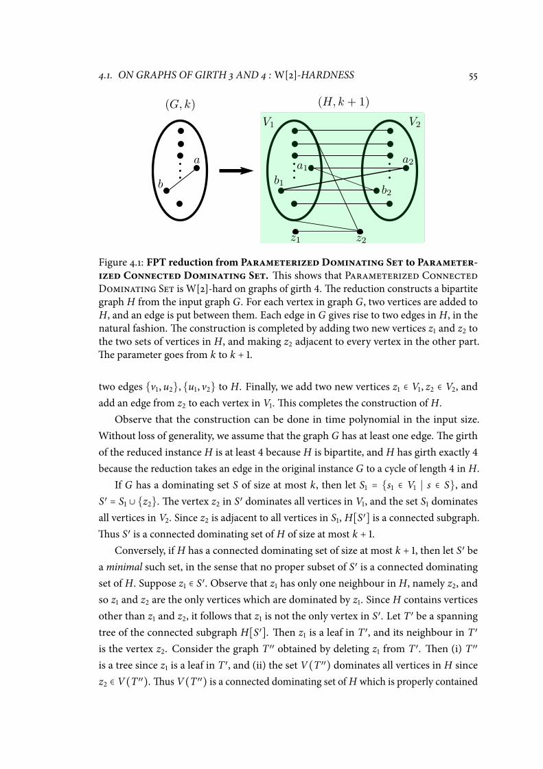
4.1. ON GRAPHS OF GIRTH 3 AND 4 :W[2]-HARDNESS 55
Figure 4.1: FPT reduction from ParameterizedDominating Set to Parameter-ized Connected Dominating Set. is shows that Parameterized ConnectedDominating Set is W[2]-hard on graphs of girth 4.e reduction constructs a bipartite
graph H from the input graph G. For each vertex in graph G, two vertices are added to
H, and an edge is put between them. Each edge in G gives rise to two edges in H, in the
natural fashion.e construction is completed by adding two new vertices z1 and z2 to
the two sets of vertices in H, and making z2 adjacent to every vertex in the other part.
e parameter goes from k to k + 1.
two edges v1, u2, u1, v2 to H. Finally, we add two new vertices z1 ∈ V1, z2 ∈ V2, and
add an edge from z2 to each vertex in V1.is completes the construction of H.
Observe that the construction can be done in time polynomial in the input size.
Without loss of generality, we assume that the graph G has at least one edge.e girth
of the reduced instance H is at least 4 because H is bipartite, and H has girth exactly 4
because the reduction takes an edge in the original instance G to a cycle of length 4 in H.
If G has a dominating set S of size at most k, then let S1 = s1 ∈ V1 ∣ s ∈ S, and
S′ = S1 ∪ z2.e vertex z2 in S′ dominates all vertices in V1, and the set S1 dominates
all vertices in V2. Since z2 is adjacent to all vertices in S1, H[S′] is a connected subgraph.
us S′ is a connected dominating set of H of size at most k + 1.
Conversely, if H has a connected dominating set of size at most k + 1, then let S′ be
aminimal such set, in the sense that no proper subset of S′ is a connected dominating
set of H. Suppose z1 ∈ S′. Observe that z1 has only one neighbour in H, namely z2, and
so z1 and z2 are the only vertices which are dominated by z1. Since H contains vertices
other than z1 and z2, it follows that z1 is not the only vertex in S′. Let T ′ be a spanning
tree of the connected subgraph H[S′]. en z1 is a leaf in T ′, and its neighbour in T ′
is the vertex z2. Consider the graph T ′′ obtained by deleting z1 from T ′. en (i) T ′′
is a tree since z1 is a leaf in T ′, and (ii) the set V(T ′′) dominates all vertices in H since
z2 ∈ V(T ′′).us V(T ′′) is a connected dominating set ofH which is properly contained

56 CHAPTER 4. CONNECTED DOMINATION AND GIRTH
in S′, which contradicts the assumption that S′ is a minimal connected dominating set of
H.erefore z1 ∉ S′, and since S′ dominates z1, it follows that z2 ∈ S′.
us S′ consists of z2, some vertices in V1, and possibly some vertices in V2. Now let
S = u ∣ u ∈ V(G);u1 ∈ S′ or u2 ∈ S′. Observe that the natural projection from S′ ∖ z2
to S is many-to-one and onto. Hence there are at most k vertices in S. Now consider
any vertex v ∈ V(G) ∖ S. Since S′ is a dominating set of the graph H, the vertex v2 in
H is dominated by some vertex u1 ∈ (V1 ∩ S′). From the construction of H, this implies
that the edge u, v is present in the graph G, and from the denition of S, it follows that
u ∈ S.us the vertex v is adjacent to some vertex u ∈ S, in the graph G. Since this holds
for any vertex v ∉ S, it follows that S is a dominating set of G of size at most k.us the
reduction is sound, and so the Parameterized Connected Dominating Set problem
is W[2]-hard when restricted to graphs of girth 4.
To see that Parameterized Connected Dominating Set is W[2]-hard on graphs
of girth 3 as well, modify the construction of H as follows: Add a new vertex z3 and the
two edges z2, z3, z1, z3 to H to form a triangle. Now H has girth 3, and the reduced
instance is (H, k + 1). Essentially the same argument as above shows that this reduction
is sound.
4.2 On Graphs of Girth 5 or More : A Kernel of Size 2kk3k
Recall thatGr denotes the set of all graphs with girth at least r ∈ N. As we show later in thischapter (see Lemma 4.7), the Parameterized Connected Dominating Set problem
remains NP-complete in graphs which do not have cycles of length 3 or 4 — that is, on
G5. We now show that the Parameterized Connected Dominating Set problemis xed-parameter tractable and can be solved in 2kk3knO(1) time on G5. It follows afolklore theorem of parameterized complexity (See Chapter 2,eorem 2.1.) that the
Parameterized Connected Dominating Set problem restricted toG5 has a kernel ofsize 2kk3k.
To show that Parameterized Connected Dominating Set is FPT onG5, we rstderive an FPT algorithm for a slightly more general, vertex-coloured version of the Para-
meterized ConnectedDominating Set problem onG5. It is straightforward to reduceParameterized Connected Dominating Set to this more general version in FPT—
in fact, polynomial — time, and thus we get an FPT algorithm for Parameterized Con-
nected Dominating Set onG5. In the more general problem, called ParameterizedConnected RWB-Dominating Set, the vertices of the input graph are partitioned into
4.2. ON GRAPHS OF GIRTH 5 OR MORE : A KERNEL OF SIZE 2KK3K 57
three colour classes, called red, white, and blue. Recall that we used such a partitioning
in Section 3.1 to obtain a polynomial kernel for the Parameterized Dominating Set
problem on Ki , j-free graphs.e general idea is similar in this case as well, but now the
colouring is subject to some constraints.is approach is motivated by a similar colour-
ing used by Raman and Saurabh to obtain a polynomial kernel for the Parameterized
Dominating Set problem onG5 graphs [102].We dene an rwb-graph (a red-white-blue graph) to be a graph whose vertices are
coloured with the three colours red, white, and blue, such that (i) every white vertex is the
neighbour of some red vertex, and (ii) blue vertices have no red neighbours. More formally,
an rwb-graph is a graph G whose vertex set V(G) is partitioned into RG ,WG , and BG —
coloured red, white, and blue, respectively — such that (i) for every w ∈WG , there is at
least one v ∈ RG such that v ,w ∈ E(G), and (ii) there is no pair v ∈ BG ,w ∈ RG such that
v ,w ∈ E(G). A connected rwb-dominating set of an rwb-graph G is a dominating set
S ⊆ V(G) of G such that (i) G[S] is connected and (ii) RG ⊆ S. Observe that, in contrast
to the denition in Section 3.1, here we stipulate that S dominate all vertices in G. We
dene the Parameterized Connected RWB-Dominating Set problem as follows:
Parameterized Connected RWB-Dominating Set
Input: An rwb-graph G, and a positive integer k.
Parameter: k
Question: Does G have a connected rwb-dominating set of size at most k?
e semantics of the colours are similar to those dened by Raman and Saurabh [102].
A vertex is coloured red if it is denitely present in the connected dominating set S that
our algorithm is trying to construct. A white vertex is one that is not yet in S but is known
to be dominated by some vertex in S. All the remaining vertices are yet to be dominated,
and are coloured blue.
We note that Raman and Saurabh claimed [102, Corollary 3] that Parameterized
Connected Dominating Set restricted toG5 has a kernel on O(k3) vertices, and hence
is xed-parameter tractable. But the argument that they present is incorrect; in fact, as we
show later (eorem 4.3), Parameterized Connected Dominating Set restricted to
G5 cannot have any polynomial-sized kernel unless the Polynomial Hierarchy collapses tothe third level.e error in their argument arises from the assumption that the reduction
rules which they use for ParameterizedDominating Set also work for Parameterized
Connected Dominating Set— but rules like deleting a white vertex or deleting edges
between white vertices do not apply to Parameterized Connected Dominating Set.
58 CHAPTER 4. CONNECTED DOMINATION AND GIRTH
is is because such vertices and edges may be needed to provide connectivity to a
dominating set. However, the xed-parameter tractability result still holds, because we
show by a dierent argument that
Lemma4.1. Ongraphs of girth at least 5, ParameterizedConnectedRWB-Dominating
Set is xed-parameter tractable and can be solved in O⋆(2kk3k) time.
We can reduce an instance of Parameterized Connected Dominating Set to an
equivalent instance of Parameterized Connected RWB-Dominating Set in polyno-
mial time, with no change in the parameter:
Lemma 4.2. An instance (G , k) of Parameterized Connected Dominating Set can
be converted to an equivalent instance (H, k) of Parameterized Connected RWB-
Dominating Set in polynomial time.
Proof. Colour all vertices of G blue to obtain the rwb-graph H.
If G has a connected dominating set S of size at most k, then the same set S is a
connected rwb-dominating set of H of size at most k : since we did not change the
structure of the graph, H[S] is connected, and S is a dominating set of H. Since the set
RH of red vertices in H is the empty set, RH ⊆ S holds vacuously.
Conversely, if S′ is a connected rwb-dominating set ofH of size at most k, then sinceG
andH are isomorphic as graphs (ignoring the colours), S′ itself is a connected dominating
set of G of size at most k.
Observe that the construction in Lemma 4.2 does not decrease the girth of the input
graph, since it does not change the structure of the graph at all. To solve the Para-
meterized Connected Dominating Set problem on G5 in FPT time, we rst applyLemma 4.2 to the input instance to obtain an equivalent Parameterized Connected
RWB-Dominating Set instance where the underlying graph has girth at least 5. We then
solve this instance of Parameterized Connected RWB-Dominating Set in FPT time
using Lemma 4.1.us we have
eorem 4.2. Parameterized ConnectedDominating Set can be solved inO⋆(2kk3k)
time on graphs of girth at least 5.
For the reasons stated above, this directly yields
Corollary 4.1. e Parameterized Connected Dominating Set problem has a kernel
of size 2kk3k on graphs of girth at least 5.
4.2. ON GRAPHS OF GIRTH 5 OR MORE : A KERNEL OF SIZE 2KK3K 59
In the remaining part of this subsection we prove Lemma 4.1.
A key ingredient in the proof of Lemma 4.1 is the fact that if G is a graph of girth at
least 5, then every vertex in G with degree more than k is present in every dominating set
of G of size at most k. To see this, observe rst that the neighbours of any vertex in G
form an independent set, or else there would be a triangle in G. Further, no two vertices
u, v ∈ V(G) can have more than one common neighbour. For, if x , y are two common
neighbours of u and v, then u, v , x , y form a cycle of length 4 in G.us we have:
Observation 1. If G is a graph of girth at least 5, then the open neighbourhood N(v) of
any vertex v ∈ V(G) is an independent set, and no two vertices of G have more than one
common neighbour.
is observation implies that if a vertex v ∈ V(G) with degree more than k is not
allowed to be picked as part of a dominating set of G, then we need more than k vertices
to dominate all the vertices in G:
Lemma 4.3. Let G be a graph of girth at least 5. If a vertex v in G has more than k
neighbours, then v is present in every dominating set of G of size at most k.
Proof. Assume for the sake of contradiction that S is a dominating set of G of size at most
k such that v ∉ S.en N(v) ∩ S ≠ ∅, or else S does not dominate v. Let ∣N(v) ∩ S∣ = ℓ.
en 1 ≤ ℓ ≤ k, and ∣N(v) ∖ S∣ ≥ k + 1 − ℓ. Since G[N(v)] is an independent set as per
Observation 1, none of the vertices in N(v) ∖ S is dominated by any of the ℓ vertices in
N(v)∩ S. Hence all the (at least k + 1− ℓ) vertices in N(v) are dominated by at most k − ℓ
vertices from S ∖ N[v].is is clearly impossible if ℓ = k, and so ℓ < k.us — by the
pigeonhole principle — there is at least one vertex u ∈ (S ∖ N[v]) that dominates at least
two vertices x , y in N(v).e vertices u, v thus have two common neighbours x , y in G,
which contradicts Observation 1.
A second key ingredient in the proof of Lemma 4.1 is the existence of an FPT algorithm
for the Parameterized Steiner Tree problem, which is a parameterized version of the
classical Steiner Tree problem. Let H be a graph and T ⊆ V(H) a set of designated
“terminal” vertices ofH. A Steiner tree ofH for the terminal set T is a connected subgraph
of H with the minimum number of edges which includes all the terminal vertices; it is
easy to see that such a subgraph, if it exists, is a tree.e Steiner Tree problem is dened
as follows:
Steiner Tree
Input: A graph H, a set T ⊆ V(H) of designated “terminal” vertices, and a
positive integer c.
60 CHAPTER 4. CONNECTED DOMINATION AND GIRTH
Question: Does H have a Steiner tree for the terminal set T , with at most c edges?
e Steiner Tree problem is NP-hard; in fact, it is one among Karp’s original list [75]
of 21 NP-complete problems. Of interest to us is the parameterized version of the problem
where the parameter is ∣T ∣, the number of terminals:
Parameterized Steiner Tree
Input: A graph H, a set T ⊆ V(H) of designated “terminal” vertices, and a
positive integer c.
Parameter: ∣T ∣
Question: Does H have a Steiner tree for the terminal set T , with at most c edges?
is problem is FPT. In fact, an FPT algorithm for this problem predates the invention
of the notion of parameterized complexity. e classical algorithm for Steiner Tree
due to Dreyfus and Wagner [43] from the year 1972 solves the problem in O⋆(3∣T ∣) time.
Aer many improvements, the current fastest FPT algorithm for the problem, due to
Nederlof [94], runs in O⋆(2∣T ∣) time and polynomial space.
Fact 1. [94]e Parameterized Steiner Tree problem can be solved in O⋆(2∣T ∣) time
and polynomial space. Further, if the input graph H contains a Steiner tree for the terminal
set T with at most c edges, then such a Steiner tree can be found within the same time
bound.
We are now ready to prove Lemma 4.1.
Proof of Lemma 4.1. Let (G , k) be an instance of Parameterized Connected RWB-
Dominating Set where G has girth at least 5. Let A be the set of white and blue vertices
in G, each of which has at least k + 1 neighbours. By Lemma 4.3, every vertex in A is part
of every dominating set — connected or otherwise — of G of size at most k.erefore, if
∣RG ∪A∣ > k then G does not have any dominating set of size at most k which contains all
the vertices of RG .e algorithm nds this set A and returns No if ∣RG ∪ A∣ > k.is can
be done in polynomial time, and henceforth we assume that ∣RG ∪ A∣ ≤ k.
e algorithm now colours all the vertices of the set A red, and all the blue neighbours
of these vertices white.is can be done in polynomial time, and from Lemma 4.3, the
resulting instance is equivalent to the original instance. Observe that the resulting graph
is also an rwb-graph. To keep the notation simple, we use G to refer to this resulting
graph as well.
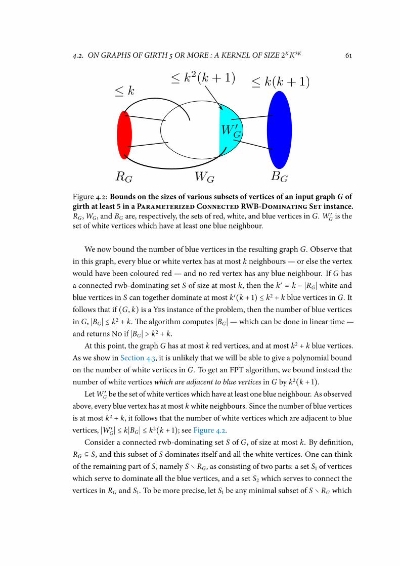
4.2. ON GRAPHS OF GIRTH 5 OR MORE : A KERNEL OF SIZE 2KK3K 61
Figure 4.2: Bounds on the sizes of various subsets of vertices of an input graph G ofgirth at least 5 in a Parameterized Connected RWB-Dominating Set instance.RG ,WG , and BG are, respectively, the sets of red, white, and blue vertices in G.W
′
G is the
set of white vertices which have at least one blue neighbour.
We now bound the number of blue vertices in the resulting graph G. Observe that
in this graph, every blue or white vertex has at most k neighbours — or else the vertex
would have been coloured red — and no red vertex has any blue neighbour. If G has
a connected rwb-dominating set S of size at most k, then the k′ = k − ∣RG ∣ white and
blue vertices in S can together dominate at most k′(k + 1) ≤ k2 + k blue vertices in G. It
follows that if (G , k) is a Yes instance of the problem, then the number of blue vertices
in G, ∣BG ∣ ≤ k2 + k.e algorithm computes ∣BG ∣—which can be done in linear time —
and returns No if ∣BG ∣ > k2 + k.
At this point, the graph G has at most k red vertices, and at most k2 + k blue vertices.
As we show in Section 4.3, it is unlikely that we will be able to give a polynomial bound
on the number of white vertices in G. To get an FPT algorithm, we bound instead the
number of white vertices which are adjacent to blue vertices in G by k2(k + 1).
LetW ′
G be the set of white vertices which have at least one blue neighbour. As observed
above, every blue vertex has at most k white neighbours. Since the number of blue vertices
is at most k2 + k, it follows that the number of white vertices which are adjacent to blue
vertices, ∣W ′
G ∣ ≤ k∣BG ∣ ≤ k2(k + 1); see Figure 4.2.
Consider a connected rwb-dominating set S of G, of size at most k. By denition,
RG ⊆ S, and this subset of S dominates itself and all the white vertices. One can think
of the remaining part of S, namely S ∖ RG , as consisting of two parts: a set S1 of vertices
which serve to dominate all the blue vertices, and a set S2 which serves to connect the
vertices in RG and S1. To be more precise, let S1 be any minimal subset of S ∖ RG which
62 CHAPTER 4. CONNECTED DOMINATION AND GIRTH
dominates BG , and let S2 = S ∖ (RG ∪ S1).e algorithm guesses the subset S1, and veries
the guess by computing the set S2 and checking if ∣S2∣ ≤ k − ∣RG ∪ S2∣.
To see how the inclusion-minimal set S1 which dominates BG can be computed in
FPT time, observe that no vertex in RG ∪ (WG ∖W ′
G) can dominate any blue vertex. It
follows that the only vertices which can be part of the set S1 are those present in BG ∪W ′
G .
In other words, S1 ⊆ (BG ∪W′
G).e algorithm guesses the set S1 by trying out each subset
of BG ∪W ′
G of size at most k − ∣RG ∣. Since ∣(BG ∪W ′
G)∣ ≤ k(k + 1)2, this can be done in
O((k(k+1)2
k−∣RG ∣)) = O(k3k) time.
It is clear from the above discussion that to verify a given guess for the set S1, it is
necessary and sucient to ensure two things, namely: (i) the set RG ∪ S1 is a dominating
set of G, and (ii) there exists a set S2 ⊆ V(G) ∖ (RG ∪ S1) such that G[R ∪ S1 ∪ S2] is
a connected subgraph and ∣R ∪ S1 ∪ S2∣ ≤ k. It is straightforward to see that the rst
condition can be checked in polynomial time.
To check the second condition, wemake use of the FPT algorithm for Parameterized
Steiner Tree from Fact 1. We create an instance of Parameterized Steiner Tree as
follows: the input graph is G itself, the terminal set T = RG ∪ S1, and the budget c = k − 1.
We now invoke the algorithm of Fact 1 to solve this instance in O⋆(2∣T ∣) = O⋆(2k) time.
If the algorithm nds a Steiner tree TS of G on the terminal set T and with at most
k − 1 edges, then the vertex set V(TS) of this Steiner tree is a connected rwb-dominating
set of G of size at most k: Since T = RG ∪ S1 ⊆ V(TS), V(TS) dominates all vertices in
G. e subgraph G[V(TS)] is connected, as witnessed by the spanning tree TS of this
subgraph. RG ⊆ V(TS), and since the tree TS has at most k − 1 edges, ∣V(TS)∣ ≤ k.
Conversely, if there exists a set S2 ⊆ V(G) ∖ (RG ∪ S1) such that G[R ∪ S1 ∪ S2] is a
connected subgraph and ∣R ∪ S1 ∪ S2∣ ≤ k, then any spanning tree of G[R ∪ S1 ∪ S2] is a
Steiner tree of G on the terminal set T = RG ∪ S1 and with at most k − 1 edges, and so the
algorithm of Fact 1 will nd such a Steiner tree TS .
erefore, to verify a given guess for the set S1, our algorithm for Parameter-
ized Connected RWB-Dominating Set runs the FPT algorithm for Parameterized
Steiner Tree from Fact 1. If this latter algorithm returns No, then our algorithm rejects
this guess for S1. Otherwise it returns the vertex set of the Steiner tree found as a connected
rwb-dominating set of G of size at most k. If all guesses for the set S1 are rejected, then
our algorithm returns No.
e correctness of our algorithm is clear from the above discussion. To bound its
running time, observe that apart from guessing the set S1 and verifying the guess, all the
other steps in the algorithm can be done in polynomial time. As described above, the
number of dierent possibilities for the set S1 is O(k3k), and all these possibilities can be
enumerated in O(k3k) time. For each subset S1, the size of the terminal set T = RG ∪ S1
4.3. ON GRAPHS OF GIRTH 5 AND 6: NO POLYNOMIAL KERNELS 63
which occurs in the Parameterized Steiner Tree problem is at most k, and so this
problem can be solved in O⋆(2k) time. us the total time taken by the algorithm is
bounded by O⋆(2kk3k).is concludes the proof of theorem.
4.3 On Graphs of girth 5 and 6: No Polynomial Kernels
In the previous section, we saw how the Parameterized Connected Dominating
Set problem is FPT and has a kernel of size O⋆(2kk3k) onG5.e next natural questionto ask is whether Parameterized Connected Dominating Set has a polynomial
kernel on G5. In this section, we answer this question in the negative: we show thatParameterized Connected Dominating Set restricted to graphs of girth 5 or 6 does
not have a polynomial kernel unless the Polynomial Hierarchy collapses to the third level.
To this end, we use various notions and results from the recently developed theory of
kernel lower bounds [15, 18, 39]; these are described in Section 2.2.1.
4.3.1 Kernel Lower Bounds for PARAMETERIZED CONNECTED DOMINAT-ING SET
As we show later in this section, the derived classical problem— the “unparameterized”
version — of Parameterized Connected Dominating Set is NP-complete when
restricted toG5. Byeorem 2.2, to show that ParameterizedConnectedDominatingSet has no polynomial kernels∗ on graphs of girth at least 5, it is sucient to exhibit a
composition algorithm for the problem on this class of graphs. Unfortunately, this task
turns out to be quite hard, and we have not been able to devise a composition algorithm for
this problem. To get around this diculty, we make use of the second tool for obtaining
kernel lower bounds, namely polynomial parameter transformations (See Section 2.2.1)
andeorem 2.3. We introduce an intermediate problem, named Parameterized Fair
Connected Colours, and show that its unparameterized version is NP-complete.e
Parameterized Fair Connected Colours problem is easy to compose, and hence
byeorem 2.2, it has no polynomial kernel. We then give a polynomial parameter
transformation from Parameterized Fair Connected Colours to Parameterized
Connected Dominating Set in G6, which implies, byeorem 2.3, that the latterproblem has no polynomial kernel. A small modication in the reduction yields the same
negative result for Parameterized Connected Dominating Set onG5 as well.
∗ Unless CoNP ⊆ NP/Poly and the Polynomial Hierarchy collapses to the third level; see Chapter 2. For easein reading, we drop the mention of this condition from now onwards; it is to be taken as being implicitly
present whenever we mention the absence of polynomial kernels.
64 CHAPTER 4. CONNECTED DOMINATION AND GIRTH
Recently, Cygan et al showed that the Parameterized Connected Dominating
Set problem does not have polynomial kernels on graphs of bounded degeneracy [28].
In order to do this, they introduced a new problem named Parameterized Connected
Colours which “nicely encapsulates the hardness of the connectivity requirement”.
Parameterized Connected Colours
Input: A graph G = (V , E), where the vertices V are (arbitrarily) coloured with
k colours.Parameter: k
Question: Does G contain a tree T on k vertices as a subgraph, where each vertex
of T has a distinct colour?
For our purpose we dene a variant of this problem, which we call Parameterized
Fair Connected Colours. An assignment of colours to the vertices of a graph is said
to be proper if the two end points of each edge in the graph have distinct colours.e
colouring is said to be fair if all neighbours of each vertex in the graph receive distinct
colours. In Parameterized Fair Connected Colours, the input graph is properly and
fairly coloured:
Parameterized Fair Connected Colours
Input: A graphG, where the vertices V(G) are properly and fairly coloured with
k colours.Parameter: k
Question: Does G contain a tree T on k vertices as a subgraph, where each vertex
of T has a distinct colour?
e unparameterized version of this problem is NP-complete, by reduction from CNF
SAT.
Lemma 4.4. e derived classical problem associated with Parameterized Fair Con-
nected Colours problem is NP-complete.
Proof. Note that the input to the derived classical problem associated with Parameter-
ized Fair Connected Colours consists of the input of Parameterized Fair Con-
nected Colours, together with a unary encoding of the number k.e question is the
same as that for Parameterized Fair Connected Colours. Let T be a subgraph of the
input graph G such that T is a tree on k vertices which has all its vertices coloured with
distinct colours. Such a subgraph T constitutes a polynomial-time veriable witness to a
4.3. ON GRAPHS OF GIRTH 5 AND 6: NO POLYNOMIAL KERNELS 65
Yes-instance of the problem, and so the Parameterized Fair Connected Colours
problem is in NP.
To show NP-hardness, we reduce from the NP-complete CNF SAT problem [75]. In
the CNF SAT problem, the input is a Boolean formula in conjunctive normal form— it is
an “AND” of clauses, where each clause is an “OR” of (positive or negative) literals — and
the question is whether there is an assignment of 0, 1 values to the variables of the formula
such that the formula evaluates to 1. Let ϕ be a Boolean formula in conjunctive normal
form, on the variables x1, . . . , xn and with clauses C1, . . . ,Cm. If a clause contains both a
variable and its negation, then we can safely remove the clause and solve the problem on
the remaining formula, since this clause evaluates to 1 for any assignment of values to the
variables. So we assume, without loss of generality, that there is no clause that contains
both a variable and its negation.
Given ϕ, we construct a graph∗ G onm + 2n + 3 vertices as follows, where the vertices
are coloured using m + n + 3 colours. We add one vertex for each variable in ϕ, one for
the negation of each variable, one for each clause, and three special vertices named r, a, b.
at is, we dene the vertex set to be V(G) ∶= r, a, b, x1, . . . , xn , x1, . . . , xn ,C1, . . . ,Cm.
We add edges joining r to a and b, edges from a to each “variable” vertex, from b to each
“negated variable” vertex, and from each “clause” vertex to the vertices corresponding to
all the literals which appear in the clause. at is, we add the edges r, a, r, b and
a, x1, a, x2, . . . , a, xn, b, x1, b, x2, . . . , b, xn, and for each vertex Ci , we add
an edge from Ci to vertex y ∈ x1, . . . , xn , x1, . . . , xn if and only if the literal y appears in
clause Ci in the formula ϕ.is completes the construction of the graph G. We assign the
colours 0,+,− to vertices r, a, b, respectively. For 1 ≤ i ≤ n, we assign colour i to vertices
xi and xi , and for 1 ≤ j ≤ m, we assign colour n + j to vertex C j. Finally†, we append a
unary encoding of the numberm+n+3 to the encoding of this graph.is completes the
construction; see Figure 4.3 for an illustration of the coloured graph in the construction.
Note that both the neighbours of the vertex r have distinct colours which are dierent
from the colour of the vertex r. Similarly, all the neighbours of the vertex a have distinct
colours dierent from the colour of a, and so also for b and each of the vertices xi and xi .
Since no clause contains both a variable and its negation, the same holds for all the “clause”
vertices Ci as well.us the vertices of G are properly and fairly coloured with n +m + 3
colours.e reduced instance of the unparameterized version of Parameterized Fair
Connected Colours is (G#m + n + 3), where # is a special symbol and the number
∗ is graph is somewhat similar to the clause-variable incidence graph of the formula ϕ.
† To meet the requirement stated in the denition of a derived classical problem— see Section 2.2.1.
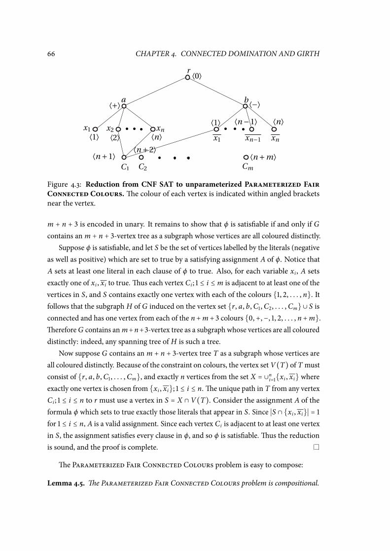
66 CHAPTER 4. CONNECTED DOMINATION AND GIRTH
Figure 4.3: Reduction from CNF SAT to unparameterized Parameterized FairConnected Colours. e colour of each vertex is indicated within angled bracketsnear the vertex.
m + n + 3 is encoded in unary. It remains to show that ϕ is satisable if and only if G
contains an m + n + 3-vertex tree as a subgraph whose vertices are all coloured distinctly.
Suppose ϕ is satisable, and let S be the set of vertices labelled by the literals (negative
as well as positive) which are set to true by a satisfying assignment A of ϕ. Notice that
A sets at least one literal in each clause of ϕ to true. Also, for each variable xi , A sets
exactly one of xi , xi to true.us each vertex Ci ; 1 ≤ i ≤ m is adjacent to at least one of the
vertices in S, and S contains exactly one vertex with each of the colours 1, 2, . . . , n. It
follows that the subgraph H of G induced on the vertex set r, a, b,C1,C2, . . . ,Cm∪ S is
connected and has one vertex from each of the n+m+ 3 colours 0,+,−, 1, 2, . . . , n+m.
ereforeG contains anm+n+3-vertex tree as a subgraph whose vertices are all coloured
distinctly: indeed, any spanning tree of H is such a tree.
Now suppose G contains an m + n + 3-vertex tree T as a subgraph whose vertices are
all coloured distinctly. Because of the constraint on colours, the vertex setV(T) of T must
consist of r, a, b,C1, . . . ,Cm, and exactly n vertices from the set X = ∪ni=1xi , xi where
exactly one vertex is chosen from xi , xi; 1 ≤ i ≤ n.e unique path in T from any vertex
Ci ; 1 ≤ i ≤ n to r must use a vertex in S = X ∩ V(T). Consider the assignment A of the
formula ϕ which sets to true exactly those literals that appear in S. Since ∣S ∩ xi , xi∣ = 1
for 1 ≤ i ≤ n, A is a valid assignment. Since each vertex Ci is adjacent to at least one vertex
in S, the assignment satises every clause in ϕ, and so ϕ is satisable.us the reduction
is sound, and the proof is complete.
e Parameterized Fair Connected Colours problem is easy to compose:
Lemma 4.5. e Parameterized Fair Connected Colours problem is compositional.
4.3. ON GRAPHS OF GIRTH 5 AND 6: NO POLYNOMIAL KERNELS 67
Proof. e composition consists of merely computing the disjoint union of the input
graphs.at is, given t instances (G1, k), (G2, k), . . . , (Gt , k) of Parameterized Fair
Connected Colours, the composition algorithm constructs the disjoint union G =
∪ti=1Gi , and returns the instance (G , k). If at least one of the input instances is a Yes
instance, then the k-coloured tree from that instance survives intact in G as well, and so
(G , k) is a Yes instance. Conversely, if (G , k) is a Yes instance, then any k-coloured tree
on k vertices that is a subgraph of G cannot span two dierent connected components
of G, and so must appear intact in some graph Gi in the input; (Gi , k) is then a Yes
instance.
Fromeorem 2.2, Lemma 4.4, and Lemma 4.5 we get:
Lemma 4.6. e Parameterized Fair Connected Colours problem does not have a
polynomial kernel unless the Polynomial Hierarchy collapses to the third level.
Wenowprove ourmain result by giving a polynomial parameter transformation (PPT)
from Parameterized Fair Connected Colours to Parameterized Connected
Dominating Set on graphs with girth 5 or 6. Recall — Denition 2.4 — that such a
transformation runs in polynomial time and constructs an equivalent instance with a
polynomially bounded parameter.
eorem 4.3. e Parameterized Connected Dominating Set problem restricted to
graphs of girth 5 or 6 does not admit a polynomial kernel unless the Polynomial Hierarchy
collapses to the third level.
Proof. Note that byeorem 2.3 and Lemma 4.6 it is sucient to show that there is a
polynomial parameter transformation (PPT) from Parameterized Fair Connected
Colours to each of these problems. We rst describe a PPT from Parameterized Fair
Connected Colours to Parameterized Connected Dominating Set on graphs of
girth six. Given an instance (G , k) of Parameterized Fair Connected Colours, we
construct an instance (H, k′) of Parameterized Connected Dominating Set where
H has girth six and k′ is bounded by a polynomial in k.
We start with a copy of G. For each colour class (set of vertices of the same colour) Ci
of G, we add a new vertex vi adjacent to all vertices of Ci , and a new vertex дi adjacent
to vi . e vertex дi is essentially a guard vertex that will force vi to be selected in any
solution (to the Parameterized Connected Dominating Set instance). We add a
new vertex uv for each edge u, v of G, and replace the edge u, v by two new edges
u, uv, uv , v.at is, we split each edge of G once.is helps to ensure that the girth
of the resulting graph is more than four. For every pair of colour classes Ci ,C j; i < j of G,
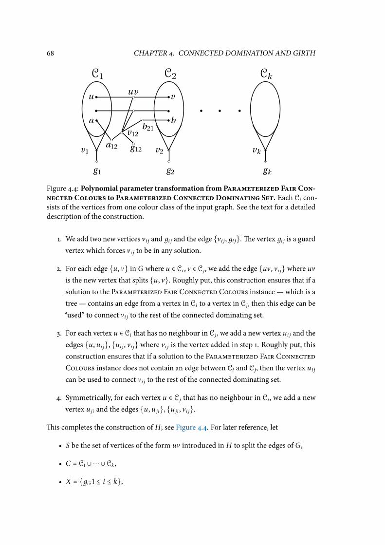
68 CHAPTER 4. CONNECTED DOMINATION AND GIRTH
Figure 4.4: Polynomial parameter transformation from Parameterized Fair Con-nected Colours to Parameterized ConnectedDominating Set. Each Ci con-
sists of the vertices from one colour class of the input graph. See the text for a detailed
description of the construction.
1. We add two new vertices vi j and дi j and the edge vi j, дi j.e vertex дi j is a guard
vertex which forces vi j to be in any solution.
2. For each edge u, v in G where u ∈ Ci , v ∈ C j, we add the edge uv , vi j where uv
is the new vertex that splits u, v. Roughly put, this construction ensures that if a
solution to the Parameterized Fair Connected Colours instance — which is a
tree — contains an edge from a vertex in Ci to a vertex in C j, then this edge can be
“used” to connect vi j to the rest of the connected dominating set.
3. For each vertex u ∈ Ci that has no neighbour in C j, we add a new vertex ui j and the
edges u, ui j, ui j, vi j where vi j is the vertex added in step 1. Roughly put, this
construction ensures that if a solution to the Parameterized Fair Connected
Colours instance does not contain an edge between Ci and C j, then the vertex ui j
can be used to connect vi j to the rest of the connected dominating set.
4. Symmetrically, for each vertex u ∈ C j that has no neighbour in Ci , we add a new
vertex u ji and the edges u, u ji, u ji , vi j.
is completes the construction of H; see Figure 4.4. For later reference, let
• S be the set of vertices of the form uv introduced in H to split the edges of G,
• C = C1 ∪⋯ ∪ Ck,
• X = дi ; 1 ≤ i ≤ k,

4.3. ON GRAPHS OF GIRTH 5 AND 6: NO POLYNOMIAL KERNELS 69
• Y = vi j; 1 ≤ i < j ≤ k,
• Z = v1, v2, . . . , vk,
• W = дi j; 1 ≤ i < j ≤ k,
• U be the set of all new vertices added in steps (3) and (4) above.
Let A = C ∪ X ∪ Y , B = S ∪U ∪W ∪ Z.en
1. A∪ B is the vertex set of the constructed graph H— all the original vertices in the
graph G are present in C, and all the vertices added by the construction are present
in one of the other sets.
2. H[A] is an independent set:
(a) Every edge which was present inG between two vertices in the set C is split by
the construction, and so C is an independent set in H. From the construction,
the sets X and Y are independent sets as well.
(b) ere is no edge from any vertex in C to any vertex in X ∪ Y : the latter set
consists entirely of newly added vertices, and the construction does not add
edges from C to any vertex in X ∪ Y .
(c) e only neighbour of each дi ∈ X is the corresponding vertex vi ∉ Y . Hence
there is no edge between X and Y .
3. H[B] is an independent set.
(a) Each of the vertex sets S ,U ,W , Z is an independent set, and
(b) e construction adds no edges between any of these vertex sets.
usH is bipartite with the bipartition A⊎B. Hence every cycle inH is of even length,
and the smallest cycle has length at least 4. Also, H contains a 4-cycle if and only if there
are two vertices in A which have two common neighbours in V(H) ∖ A. But no two
vertices in A can have two common neighbours, as we argue below:
• e vertices in X are all of degree exactly one, and so they are not part of any cycle.
• In each of the remaining ways of forming a pair a, b of vertices from A, a and b
have at most one common neighbour:
– Any two vertices a, b ∈ Y are at a distance of 4 from each other, so they haveno common neighbour.

70 CHAPTER 4. CONNECTED DOMINATION AND GIRTH
– For any colour class Ci , two vertices a, b ∈ Ci have exactly one common
neighbour, namely vi .
– For two distinct colour classes Ci ,C j, let a ∈ Ci , b ∈ C j. If a, b are not adjacent
in G, then they have no common neighbour in H. Otherwise, the new vertex
that splits the edge a, b is their only common neighbour in H.
– e only remaining possibility is a ∈ C , b ∈ Y . Without loss of generality, let
a ∈ Ci , b = vi j. Since G is fairly coloured, the vertex a has either no neighbour
or has exactly one neighbour (say a′) in C j. In either case, a and b share
exactly one neighbour, namely the new vertex (named ai j or aa′, respectively)
added to H to denote the presence or absence of such a neighbour in C j.
It follows that H does not contain a 4-cycle, and so the smallest cycle in H has length at
least 6. To see that the girth of H is indeed 6, note that we can assume without loss of
generality that C1 contains at least two vertices, say a, b. Observe that there is a path of
length two from a to v12, and a path of length two from v12 to b.ese paths meet only
at v12, and together with the two edges b, v1, v1, a they form a cycle of length 6. Let
(H, k2 + k) be the reduced instance. Now we argue that the reduction is sound.
Forward direction. Suppose G contains a tree T on k vertices, where each vertex of
T has a distinct colour. Let V(T) = t1, t2, . . . , tk, where ti ∈ Ci for all i. Let T ′ be the
“corresponding” tree in H: the vertex set of T ′ consists of V(T) and all the new vertices
in H that split the edges of T , and the edge set consists of all the new edges formed by
splitting the edges of T .us T ′ is a tree on 2k − 1 vertices. We now add more vertices
and edges to T ′ to obtain a tree on k2 + k vertices that dominates all of H.
• For 1 ≤ i ≤ k, we add the vertex vi and the edge vi , ti to T ′.is adds k vertices.
We also add a vertex vi j for 1 ≤ i < j ≤ k.is adds (k2) new vertices.
• For 1 ≤ i < j ≤ k, if the vertex ti t j is present in T ′, then we add the edge ti t j, vi j to
T ′. Otherwise, let a = ti . We add the vertex ai j and the edges a, ai j, ai j, vi j to
T ′.is adds one vertex for each “non-edge” in T , and thus a total of (k2) − (k − 1)
new vertices to T ′.
is completes the construction of T ′. Note that T ′ is a tree on (2k − 1) + k + (k
2) +
((k
2) − (k − 1)) = k2 + k vertices. In H,
• the set vi ∣ 1 ≤ i ≤ k ⊆ V(T ′) dominates all the vertices copied over from G and
the new vertices д1, . . . , дk, and
4.3. ON GRAPHS OF GIRTH 5 AND 6: NO POLYNOMIAL KERNELS 71
• the set vi j ∣ 1 ≤ i < j ≤ k ⊆ V(T ′) dominates all the other newly added vertices.
us T ′ is a connected dominating set of H on k2 + k vertices.
Reverse direction. Let D be a minimal connected dominating set of H with 1 < ∣D∣ ≤
k2 + k. Observe rst that vertices in X ∪W are all pendant vertices, and all of their
neighbours have degree at least 2. So, using an argument similar to the one used in the
proof ofeorem 4.1, D ∩ (X ∪W) = ∅ and N(X ∪W) = (Y ∪ Z) ⊆ D. Now since
G[D] is connected and ∣D∣ ≥ 2, at least one neighbour of each vertex in D must also
be in D. Observe that for any two vertices u, v ∈ Y ∪ Z, N[u] ∩ N[v] = ∅, and so each
vertex in D can be the neighbour of at most one vertex in Y ∪ Z ⊆ D. us for each
vertex v ∈ Y ∪ Z, D contains at least one distinct vertex u ∈ (N(v) ∖ (Y ∪ Z)), and so
∣D∣ ≥ 2∣Y ∪ Z∣ = 2((k
2) + k) = k2 + k. But ∣D∣ ≤ k2 + k by assumption, and so ∣D∣ = k2 + k.
us exactly one neighbour of each vertex in Y ∪ Z is in D, and these neighbours are all
distinct. In particular, D contains exactly one vertex from each set Ci ; 1 ≤ i ≤ k. Further,
D = (Y ∪ Z) ∪ N(Y ∪ Z).
Let T1 be a spanning tree of H[D]. en ∣V(T1)∣ = ∣D∣ = k2 + k. From the above
arguments we see that all vertices in Y ∪ Z are leaves in T1, and so T2 = T1 ∖ (Y ∪ Z) is
also a tree, and ∣T2∣ = k2 + k − (k
2) − k = k(k + 1)/2. Observe that for each vertex v in Y ,
the neighbour w of v in T1 is either in U or in S. For each such v and the corresponding
vertex w,
• If w ∈ U , then w is a leaf in the tree T2; remove w from T2.
• Ifw ∈ S, thenw is either a leaf or has degree exactly two in T2. In either case, remove
w from T2. If w was not a leaf in T2, then add an edge between its two neighbours
in T2.
Observe that these steps yield a tree, say T .e tree T2 had k(k + 1)/2 vertices, and
the steps above remove exactly k(k − 1)/2 vertices from T2, one for each vertex in the
set Y . us T has exactly k vertices. Since T1 contained exactly one vertex from each
set Ci ; 1 ≤ i ≤ k, and since the above operations did not remove any of these vertices, it
follows that the vertex set of T consists of exactly one vertex of each colour. Observe that
each edge added in the construction of H has at least one end point in a vertex which
is not present in G.erefore, if such a “new” edge is present in T , then T would have
contained at least one of these “new” vertices. Since this is not the case, it follows that T
contains none of the new edges added to H by the construction.us T is (isomorphic
to) a subgraph of G. But T is a tree on k vertices where each vertex has a distinct colour,
and so (G , k) is a Yes instance of Parameterized Fair Connected Colours.

72 CHAPTER 4. CONNECTED DOMINATION AND GIRTH
Graphs of Girth 5. A small modication to the above reduction suces to show that
the Parameterized Connected Dominating Set problem has no polynomial ker-
nel on graphs of girth 5 as well: Add three new vertices a, b, c and the four new edges
required to complete the 5-cycle v1, a, b, c, д1 so that H has girth 5. e reduced in-
stance is (H, k2 + k + 2). In the argument to show that this reduction is sound, both
the directions go through exactly as above, once we observe that exactly one of the sets
v1, a, д1, v1, a, b, v1, д1, c is contained in any minimal connected dominating set of
H.
Observe that the polynomial parameter transformations described in the proof of
eorem 4.3 are in fact polynomial-time many-to-one reductions. It follows that the
Parameterized Connected Dominating Set problem is NP-hard when restricted to
graphs of girth 5 or 6.
Lemma 4.7. e Parameterized Connected Dominating Set problem isNP-complete
on graphs of girth 5 or 6.
4.4 On Graphs of girth 7 or More: A Cubic Vertex Kernel
We saw in the previous section that if cycles of length 5 or 6 are allowed in the input,
then the Parameterized Connected Dominating Set problem has no polynomial
kernel. We now show that if we disallow cycles of length at most 6 in the input, then the
problem has a kernel with O(k3) vertices. Recall the FPT algorithm for Parameterized
Connected Dominating Set of graphs of girth at least 5 — Section 4.2 — where we
partitioned the vertex set of the input graph into three “colours” red, white and blue. We
were able to bound the sizes of the red and blue sets by O(k2), but could (implicitly) give
only an exponential bound on the number of white vertices. e absence of cycles of
length less than 7 helps us get a polynomial bound on the size of the white set of vertices
as well, and this gives us a polynomial kernel for the problem on these graphs.
4.4.1 A Cubic Kernel for the Coloured Version
To show that Parameterized Connected Dominating Set has an O(k3) vertex ker-
nel on G7, we rst derive such a kernel for the Parameterized Connected RWB-Dominating Set problem which we dened in Section 4.2. As we saw in that section, it
is straightforward to reduce Parameterized Connected Dominating Set to Para-
meterized Connected RWB-Dominating Set in polynomial time, with no change in
the parameter. A reduction in the reverse direction is only slightly more involved, and
4.4. ON GRAPHS OF GIRTH 7 OR MORE: A CUBIC VERTEX KERNEL 73
can be done in polynomial time with an O(k) additive increase in the number of vertices.
is yields the desired kernel for Parameterized Connected Dominating Set. As
before, our reduction rules colour the vertices of G red, white, and blue. Red vertices are
those that must necessarily be in any connected dominating set of G of size at most k.
White vertices are those non-red vertices that are dominated by the red vertices, and blue
vertices are the rest. Recall that we use RG ,WG , BG , respectively, to denote the red, white,
and blue vertices in a graph G.
Let (G , k) be the input to Parameterized Connected Dominating Set, where
G ∈ G7. Our kernelization algorithm starts by colouring all the vertices of G blue toobtain an rwb-graph H. By the proof of Lemma 4.2, this step is sound.e algorithm
now exhaustively applies the following reduction rules in the given order:
(Rule 1) Let S be the set of blue vertices in H, each of which has at least k + 1 blue
neighbours. Colour all the vertices of S red and all the blue neighbours in N(S)
white.
(Rule 2) If ∣RH ∣ > k or ∣BH ∣ > k2 + k, then say No and stop.
(Rule 3) If H contains an isolated blue vertex, then say No and stop.
(Rule 4) If H contains a pendant blue or white vertex u adjacent to a vertex v, thenremove u from H. If v is not red, then colour v red and colour all the remaining
blue neighbours of v white.
e correctness of Rule 1 follows from Lemma 4.3; see also the rst paragraph in the
proof of Lemma 4.1.e bound obtained for ∣BG ∣ in the proof of Lemma 4.1 — see the
third paragraph of that proof — justies Rule 2. Observe that we need to include any
isolated blue vertex in the dominating set (to dominate that vertex), but as this vertex is
isolated, the resulting dominating set will not induce a connected graph.is implies that
if an isolated blue vertex is present in H, then H has no connected rwb-dominating set,
and this in turn justies Rule 3.
Let u be a pendant blue or white vertex in H, adjacent to a vertex v. Observe that at
least one of u, v must be in any dominating set of H, in order to dominate the vertex u.
Since u is a pendant vertex which is not red, it is not present in anyminimal connected
rwb-dominating set ofH.is follows by an argument similar to the one used in the proof
ofeorem 4.1.us the vertex v is present in every minimal connected rwb-dominating
set of H, and this justies Rule 4.
We now show how to bound ∣WH ∣ for the resulting graph H using the fact that H has
no cycles of length 6 or less.

74 CHAPTER 4. CONNECTED DOMINATION AND GIRTH
Figure 4.5: Partitioning the set of white vertices. RH ,WH , BH are, respectively, the red,
white, and blue vertex sets in the graph H.WR is the set of white vertices which have only
red neighbours.WW is the set of white vertices which have at least one white neighbour.
WB is the remaining set of white vertices, which have at least one blue neighbour.
Lemma 4.8. Let (G , k) be a Yes instance of Parameterized Connected Dominating
Set where G ∈ G7, and let H be the graph obtained from G by exhaustively applying Rule 1
to Rule 4.en ∣WH ∣ ≤ k3 + 5
2k2 − 3
2k.
Proof. As in Figure 4.5 we divideWH into three parts,WH =WB ∪WR ∪WW , where
• WB is the set of all white vertices that have at least one blue neighbour,
• WR is the set of all white vertices that have only red neighbours, and
• WW is the set of all white vertices inWH∖WB that have at least onewhite neighbour.
We now bound the size of each of these sets.
Since Rule 1 has been applied to the graph H, any blue vertex in H has degree at most
k, and so can have at most k white neighbours.us ∣WB∣ ≤ k∣BH ∣ ≤ k(k2 + k).
Since Rule 4 has been applied to H, each vertex inWR has at least two red neighbours.
Further, recall — Observation 1 — that no two vertices inH have more than one common
neighbour. It follows that ∣WR∣ ≤ (∣RH ∣
2) ≤ (
k
2). We note in passing that although the
vertices inWR do not contribute to dominating the graph, we cannot just remove these
vertices from H since they could be useful in providing connectivity in some smallest
connected dominating set.
We now bound the size of the last piece ofWH , namely the setWW of all white vertices
in WH ∖WB which have at least one white neighbour. Let EW be the set of all edges
e ∈ E(H) where both end vertices of e are white. Consider a map which associates each
vertex w ∈WW with an arbitrary edge e ∈ EW with which w is incident. Observe that this
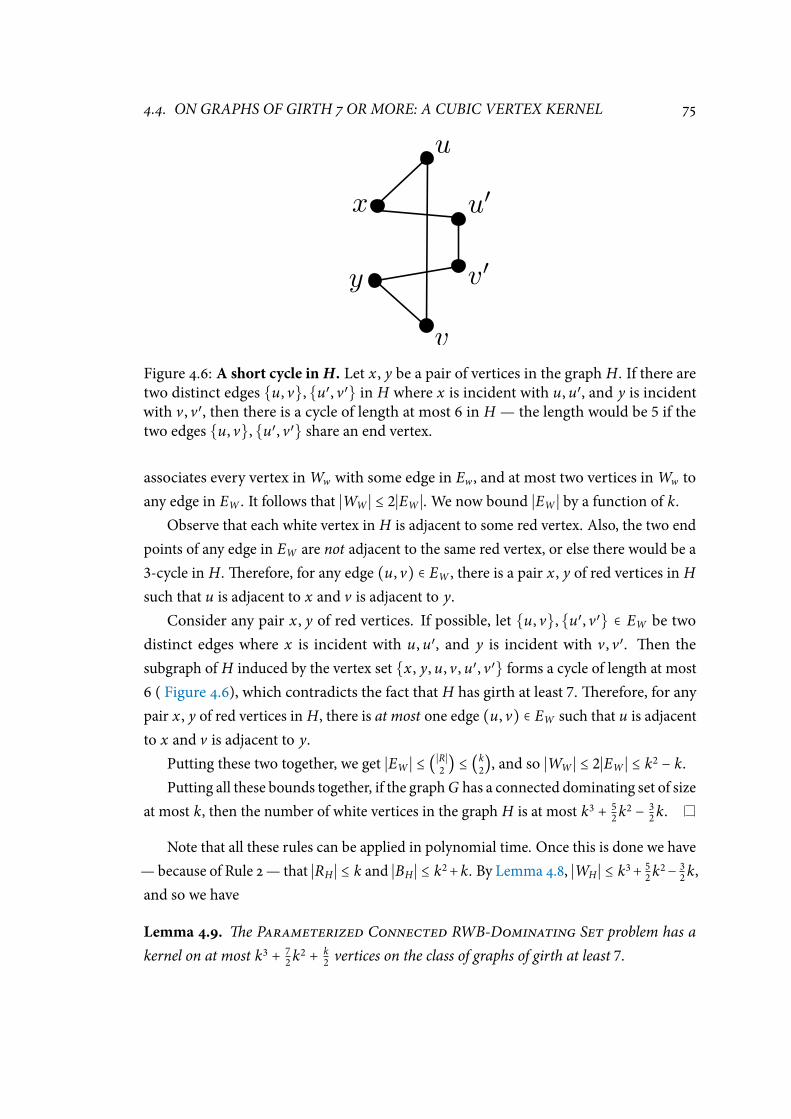
4.4. ON GRAPHS OF GIRTH 7 OR MORE: A CUBIC VERTEX KERNEL 75
Figure 4.6: A short cycle in H. Let x , y be a pair of vertices in the graph H. If there aretwo distinct edges u, v, u′, v′ in H where x is incident with u, u′, and y is incident
with v , v′, then there is a cycle of length at most 6 in H — the length would be 5 if the
two edges u, v, u′, v′ share an end vertex.
associates every vertex inWw with some edge in Ew , and at most two vertices inWw to
any edge in EW . It follows that ∣WW ∣ ≤ 2∣EW ∣. We now bound ∣EW ∣ by a function of k.
Observe that each white vertex in H is adjacent to some red vertex. Also, the two end
points of any edge in EW are not adjacent to the same red vertex, or else there would be a
3-cycle in H.erefore, for any edge (u, v) ∈ EW , there is a pair x , y of red vertices in H
such that u is adjacent to x and v is adjacent to y.
Consider any pair x , y of red vertices. If possible, let u, v, u′, v′ ∈ EW be two
distinct edges where x is incident with u, u′, and y is incident with v , v′. en the
subgraph of H induced by the vertex set x , y, u, v , u′, v′ forms a cycle of length at most
6 ( Figure 4.6), which contradicts the fact that H has girth at least 7.erefore, for any
pair x , y of red vertices in H, there is at most one edge (u, v) ∈ EW such that u is adjacent
to x and v is adjacent to y.
Putting these two together, we get ∣EW ∣ ≤ (∣R∣
2) ≤ (
k
2), and so ∣WW ∣ ≤ 2∣EW ∣ ≤ k2 − k.
Putting all these bounds together, if the graphG has a connected dominating set of size
at most k, then the number of white vertices in the graph H is at most k3 + 5
2k2 − 3
2k.
Note that all these rules can be applied in polynomial time. Once this is done we have
— because of Rule 2— that ∣RH ∣ ≤ k and ∣BH ∣ ≤ k2+k. By Lemma 4.8, ∣WH ∣ ≤ k3+ 52k2− 3
2k,
and so we have
Lemma 4.9. e Parameterized Connected RWB-Dominating Set problem has a
kernel on at most k3 + 7
2k2 + k
2vertices on the class of graphs of girth at least 7.
76 CHAPTER 4. CONNECTED DOMINATION AND GIRTH
4.4.2 Removing the Colours
Starting with an instance (G , k) of Parameterized Connected Dominating Set, let
(G′, k) be the equivalent instance of Parameterized Connected RWB-Dominating
Set obtained by applying Lemma 4.9. To obtain an instance of (uncoloured) Paramet-
erized Connected Dominating Set from this cubic vertex kernel for Parameterized
Connected RWB-Dominating Set, we do the following:
• Attach a new pendant vertex to each red vertex in G′, and,
• remove all colours from the vertices of the resulting graph to obtain a graph H.
e new instance is (H, k). Let S be a connected rwb-dominating set of the rwb-graph
G′, of size at most k. Observe that every red vertex in G′ is contained in the set S, by
denition; RG′ ⊆ S. Also, S dominates all the vertices in G′. Since all the new vertices
added to G′ are dominated by RG′ , it follows that S dominates all vertices in H as well.
Since G′[S] is connected, so is H[S], and so S is a connected dominating set of H of size
at most k.
Conversely, if S′ is a minimal connected dominating set of H of size at most k, then it
follows by the same reasoning as in the proof ofeorem 4.1 that
• no pendant vertex added during the construction is in S′, and,
• all the neighbours of these pendant vertices are in S′.
us S′ ⊆ V(G′) and RG′ ⊆ S′, and so S′ itself is a connected rwb-dominating set of G′ of
size at most k.e procedure for removing colours is thus sound, and it adds at most k
new vertices.us we get
eorem 4.4. e Parameterized Connected Dominating Set problem has a kernel
with at most k3 + 7
2k2 + 3k
2= O(k3) vertices on the class of graphs of girth at least 7.
4.5 Conclusion
In this chapter we studied the eect of excluding short cycles from the input graph,
on the kernelization complexity of the Parameterized Connected Dominating Set
problem. We obtained a diverse kernelization landscape, showing that the problem
becomes progressively easier as the girth of the input graph increases. Specically, we
show that
4.5. CONCLUSION 77
• Parameterized Connected Dominating Set is W[2]-hard on graphs which
contain cycles of length 3 or 4, and so it does not have a kernel of any size on such
graphs unless FPT=W[2].
• On any class of graphs which have girth at least 5, Parameterized Connected
Dominating Set has an FPT algorithm which runs in O(2kk3k ⋅ nc) time where n
is the number of vertices in the input graph and c is a constant independent of n
and k. As a consequence, the problem has a kernel of size 2kk3k on graphs of girth
at least 5.
• Unless the Polynomial Hierarchy (PH) collapses to the third level, Parameterized
Connected Dominating Set has no polynomial kernel on graphs which contain
cycles of length at most 6.
• On any class of graphs which have girth at least 7, Parameterized Connected
Dominating Set has a kernel on O(k3) vertices.
On the way to proving the kernel lower bound on graphs with girth at most 6 we
introduced a new problem, namely Parameterized Fair Connected Colours, and
showed that this problemhas no polynomial kernels.is intermediate result is interesting
in its own right; we feel that it could be used to show kernelization lower bounds for other
connectivity problems on graphs that exclude small cycles.
As noted before, most kernelization and FPT results for W-hard problems are for
graph classes characterized by excludedminors. Our results add to the small but growing
collection of such results for graph classes characterized by excluded subgraphs. One
interesting direction of future work is to study how the exclusion of small cycles — or
other small graphs — as subgraphs aects the kernelization complexity of other W-hard
parameterized problems.


Part III
Covering Problems
79


CHAPTER 5
Pathwidth-One Vertex Deletion
Pathwidth is a notion introduced by Robertson and Seymour in the GraphMinors
series [104] as a measure of how “path-like” a graph is. A graph has pathwidth
at most one if and only if it is a collection of caterpillars, where a caterpillar is a
special kind of tree: it is a tree that becomes a path (called the spine of the caterpillar)
when all its pendant vertices are removed. Graphs of pathwidth at most one are thus a very
special kind of forests, and have even less structure than forests (which are themselves
very “simple” graphs). As a consequence, some problems that are NP-hard even on forests
can be solved in polynomial time on graphs of pathwidth at most one. Examples include
(Weighted) Bandwidth [10, 82, 98], the Proper Interval Coloured Graph problem, and
the Proper Coloured Layout problem [6].
In this chapter we focus on the following problem : Given a graph G and an integer k
as input, nd whetherG contains a set of at most k vertices whose removal fromG results
in a graph of pathwidth atmost one. We call such a set of vertices a pathwidth-one deletion
set (PODS), and the problem the Pathwidth-OneVertexDeletion problem. It follows
from an NP-hardness “meta-result” of Lewis and Yannakakis that this problem is NP-
complete. We initiate the study of the parameterized complexity of the Pathwidth-One
Vertex Deletion problem, parameterized by the solution size k.
e Feedback Vertex Set problem is closely related to Pathwidth-One Vertex
Deletion, and has been extensively studied. A feedback vertex set (FVS) of a graph is a
set of vertices whose deletion from the graph results in a forest. Given a graph G and
an integer k as input, the Feedback Vertex Set problem asks whether G has an FVS
81

82 CHAPTER 5. PATHWIDTH-ONE VERTEX DELETION
of size at most k.is problem is NP-complete [75]. Its natural parameterized version
— with the solution size k as the parameter, which we call Parameterized Feedback
Vertex Set— is xed parameter tractable (FPT) and has a polynomial kernel.e best
known deterministic FPT algorithm for the problem [22] runs in O∗(3.83k) time, and
the smallest known kernel [107] has size O(k2).
Our Results
We show that the Pathwidth-One Vertex Deletion problem parameterized by the
solution size k—which we call Parameterized Pathwidth-One Vertex Deletion—
(i) has a kernel with O(k4) vertices, and (ii) can be solved in O∗(7k) time.
Note that, in general, a pathwidth-one deletion set “does more” than a feedback vertex
set: It “kills” all cycles in the graph, like a feedback vertex set, and, in addition, it kills
all non-caterpillar trees in the graph. In fact, the dierence in the sizes of a smallest
feedback vertex set and a smallest pathwidth-one deletion set of a graph can be arbitrarily
large. For example, the treewidth of any binary tree is 1, while for any integer c there
exists [104] a binary tree Tc of pathwidth at least c + 1. Removing a single vertex from a
graph will reduce the pathwidth by at most one, and so for Tc, the dierence between
the two numbers is at least c. Partly as a consequence of such dierences, many of the
techniques and reduction rules that have been developed for obtaining FPT algorithms
and kernels for the Parameterized Feedback Vertex Set problem do not carry over
to the Parameterized Pathwidth-One Vertex Deletion problem. Instead, we use a
characterization of graphs of pathwidth at most 1 to obtain the FPT algorithm and the
polynomial kernel.
Organization of the rest of the chapter
In Section 5.1 we show that the Parameterized Pathwidth-One Vertex Deletion
problem is NP-complete, and describe an FPT algorithm for the problem which runs in
O∗(7k) time. We show in Section 5.2 that the problem has a kernel with O(k4) vertices.
We conclude in Section 5.3.
Notation
All the graphs in this chapter are nite and undirected. In general we follow the graph
terminology of Section 2.1. A caterpillar is a tree that becomes a path (called the spine of
the caterpillar) when all its pendant vertices are removed. A nontrivial caterpillar is one
that contains at least two vertices. A T2 is the graph on seven vertices shown in Figure 5.1.
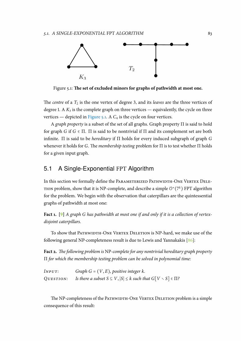
5.1. A SINGLE-EXPONENTIAL FPT ALGORITHM 83
Figure 5.1:e set of excluded minors for graphs of pathwidth at most one.
e centre of a T2 is the one vertex of degree 3, and its leaves are the three vertices of
degree 1. A K3 is the complete graph on three vertices — equivalently, the cycle on three
vertices — depicted in Figure 5.1. A C4 is the cycle on four vertices.
A graph property is a subset of the set of all graphs. Graph property Π is said to hold
for graph G if G ∈ Π. Π is said to be nontrivial if Π and its complement set are both
innite. Π is said to be hereditary if Π holds for every induced subgraph of graph G
whenever it holds forG.emembership testing problem for Π is to test whether Π holds
for a given input graph.
5.1 A Single-Exponential FPT Algorithm
In this section we formally dene the Parameterized Pathwidth-One Vertex Dele-
tion problem, show that it is NP-complete, and describe a simple O∗(7k) FPT algorithm
for the problem. We begin with the observation that caterpillars are the quintessential
graphs of pathwidth at most one:
Fact 1. [9] A graph G has pathwidth at most one if and only if it is a collection of vertex-
disjoint caterpillars.
To show that Pathwidth-One Vertex Deletion is NP-hard, we make use of the
following general NP-completeness result is due to Lewis and Yannakakis [86]:
Fact 2. e following problem isNP-complete for any nontrivial hereditary graph property
Π for which the membership testing problem can be solved in polynomial time:
Input : Graph G = (V , E), positive integer k.
Question : Is there a subset S ⊆ V , ∣S∣ ≤ k such that G[V ∖ S] ∈ Π?
e NP-completeness of the Pathwidth-OneVertexDeletion problem is a simple
consequence of this result:
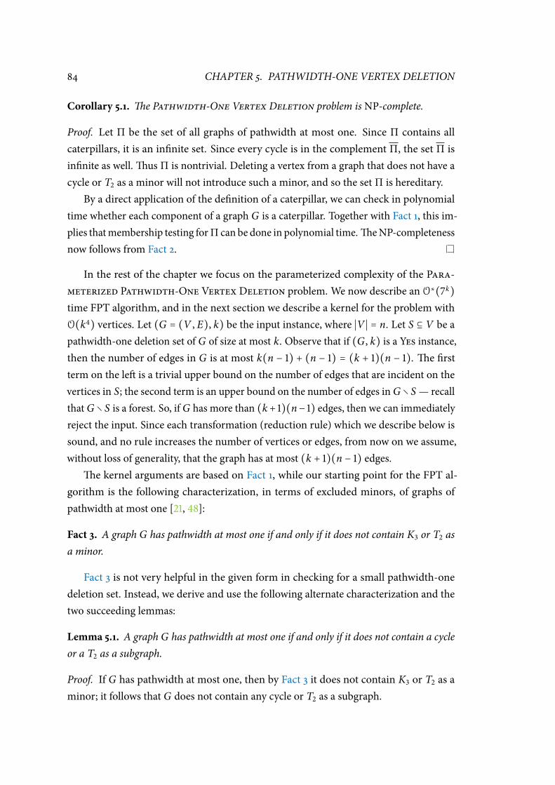
84 CHAPTER 5. PATHWIDTH-ONE VERTEX DELETION
Corollary 5.1. e Pathwidth-One Vertex Deletion problem is NP-complete.
Proof. Let Π be the set of all graphs of pathwidth at most one. Since Π contains all
caterpillars, it is an innite set. Since every cycle is in the complement Π, the set Π is
innite as well.us Π is nontrivial. Deleting a vertex from a graph that does not have a
cycle or T2 as a minor will not introduce such a minor, and so the set Π is hereditary.
By a direct application of the denition of a caterpillar, we can check in polynomial
time whether each component of a graph G is a caterpillar. Together with Fact 1, this im-
plies thatmembership testing for Π can be done in polynomial time.eNP-completeness
now follows from Fact 2.
In the rest of the chapter we focus on the parameterized complexity of the Para-
meterized Pathwidth-One Vertex Deletion problem. We now describe an O∗(7k)
time FPT algorithm, and in the next section we describe a kernel for the problem with
O(k4) vertices. Let (G = (V , E), k) be the input instance, where ∣V ∣ = n. Let S ⊆ V be a
pathwidth-one deletion set of G of size at most k. Observe that if (G , k) is a Yes instance,
then the number of edges in G is at most k(n − 1) + (n − 1) = (k + 1)(n − 1). e rst
term on the le is a trivial upper bound on the number of edges that are incident on the
vertices in S; the second term is an upper bound on the number of edges inG ∖ S— recall
thatG ∖ S is a forest. So, ifG has more than (k+ 1)(n− 1) edges, then we can immediately
reject the input. Since each transformation (reduction rule) which we describe below is
sound, and no rule increases the number of vertices or edges, from now on we assume,
without loss of generality, that the graph has at most (k + 1)(n − 1) edges.
e kernel arguments are based on Fact 1, while our starting point for the FPT al-
gorithm is the following characterization, in terms of excluded minors, of graphs of
pathwidth at most one [21, 48]:
Fact 3. A graph G has pathwidth at most one if and only if it does not contain K3 or T2 as
a minor.
Fact 3 is not very helpful in the given form in checking for a small pathwidth-one
deletion set. Instead, we derive and use the following alternate characterization and the
two succeeding lemmas:
Lemma 5.1. A graph G has pathwidth at most one if and only if it does not contain a cycle
or a T2 as a subgraph.
Proof. If G has pathwidth at most one, then by Fact 3 it does not contain K3 or T2 as a
minor; it follows that G does not contain any cycle or T2 as a subgraph.
5.1. A SINGLE-EXPONENTIAL FPT ALGORITHM 85
Conversely, assume that G does not contain a cycle or a T2 as a subgraph. Suppose G
contains a K3, say C, as a minor, obtained by contracting a set of edges E′ and deleting
a set of edges E′′ of a subgraph H of G. If we replace the contracted vertices with the
original edges E′ and add the deleted edges E′′, we obtain a cycle which is a subgraph of
the original graph (from which we obtained C as a minor), a contradiction.
Similarly, if G has a T2 as a minor, then replacing the contracted vertices with the
original edges and adding the deleted edges gives rise to a supergraph ofT2, a contradiction.
us G does not contain either K3 or T2 as a minor, and so by Fact 3 the graph G has
pathwidth at most one.
e next two lemmas imply that we can decide in polynomial time whether a graph
has pathwidth at most 1. Moreover, if the pathwidth is more than 1, then we can, in eect,
nd “all” the obstructions in polynomial time as well.
Lemma 5.2. Let S = T2,K3,C4. Given a graph G = (V , E); ∣V ∣ = n, we can nd whether
G contains a subgraph H that is isomorphic to one of the graphs in S, and also locate such
an H if it exists, in O(kn2) time.
Proof. It is well-known that we can nd the girth (length of a shortest cycle) of a graph by
doing a breadth-rst search (BFS) from each vertex.e same algorithm nds a smallest
cycle in the graph as well, and so we can use it to check for and locate a K3 or C4 in G.
Suppose G contains neither of these graphs as a subgraph. To check if G contains a T2,
we guess the centre vertex v of the T2 and do a BFS starting from v (the level 0 vertex).
Since G does not contain K3 as a subgraph, there is a T2 with v as the centre if and only
if at least three vertices in level 1 of the BFS have at least one neighbour each in level 2.
We can combine the two tests to obtain an algorithm of the required kind that runs in
O((∣V ∣)(∣V ∣ + ∣E∣)) = O(n(n + (k + 1)(n − 1))) = O(kn2) time.
A graph which does not contain any of T2,K3,C4 as a subgraph has a particularly
simple structure.
Lemma 5.3. Let S = T2,K3,C4. If G is a graph that does not contain any element of S
as a subgraph, then each connected component of G is either a tree, or a cycle with zero or
more pendant vertices (“hairs”) attached to it.
Proof. Let G be a graph that does not contain any element of S as a subgraph, and let X
be a connected component of G that is not a tree.en X contains a cycle. Let C be a
smallest cycle in X.en C has length at least 5. Suppose there is a path ⟨a, b, c⟩ in X,
where a is a vertex on C and b is not.en c ∉ V(C), or else a, b, c and the shorter path
from c to a on C form a cycle of length at most 4, a contradiction. Let x , y be the two
86 CHAPTER 5. PATHWIDTH-ONE VERTEX DELETION
neighbours of a on C, and let x′ ≠ a, y′ ≠ a be neighbours of x , y on C.en x , y, x′, y′
are all distinct, and a, b, c, x , y, x′, y′ form a T2 in X with a at the centre, a contradiction.
It follows that for any vertex u ∈ V(C), any neighbour v ∉ V(C) of u is a pendant vertex
in X, and the lemma follows.
5.1.1 An FPT algorithm for PARAMETERIZED PATHWIDTH-ONE VERTEX
DELETION
We are now ready to describe the simple FPT algorithm. Let (G = (V , E), k) be the
input instance, where ∣V ∣ = n. We use a branching strategy inspired by Lemma 5.1 and
Lemma 5.3. First we locate a (not necessarily induced) subgraph T ofG that is isomorphic
to one of S = T2,K3,C4. By Lemma 5.2, this can be done in O(kn2) time. At least one
of the (at most seven) vertices of T must be in any pathwidth-one deletion set of G. So we
branch on the vertices of T : We pick each one, in turn, into the minimal pathwidth-one
deletion set that we are constructing, delete the picked vertex and all its adjacent edges,
and recurse on the remaining graph aer decrementing the parameter by one.
e leaves of this recursion tree correspond to graphs which do not have a subgraph
isomorphic to any graph in S. By Lemma 5.3, each connected component of such a graph
is a tree, or a cycle with zero or more pendant vertices (“hairs”) attached to it.e trees
can be ignored — they do not have a T2 as a subgraph — and each cycle (with or without
hairs) forces exactly one vertex into any minimal solution. us the base case of the
recursion can be solved in linear time.
is is a 7-way branching, where the depth of the recursion is at most k, and where
the algorithm spends O(kn2) time at each node. Hence we have
eorem 5.1. e Pathwidth-One Vertex Deletion problem parameterized by the
solution size k has an FPT algorithm that runs in O(n2 ⋅ 7kk) time.
By a folklore result of parameterized complexity (SeeChapter 2), it follows immediately
fromeorem 5.1 that the Pathwidth-One Vertex Deletion problem parameterized
by the solution size k has a kernel of size O(7kk). We now show that the kernel size can
be brought down signicantly from this trivial bound.
5.2 A Quartic Kernel
We now turn to the main result of this chapter. We describe a polynomial-time al-
gorithm (the kernelization algorithm) that, given an instance (G , k) of Parameterized
Pathwidth-One Vertex Deletion, returns an instance (G′, k′) (the kernel) of Para-
meterized Pathwidth-One Vertex Deletion such that (i) (G , k) is a Yes instance

5.2. A QUARTIC KERNEL 87
Algorithm 3e kernelization algorithm1: procedure Kernelize(G , k)2: CurrentInstance ← (G , k)
3: repeat4: Apply Rule 1 to Rule 6, updating CurrentInstance with the output of each
rule.
5: until None of the rules cause any change to CurrentInstance.6: end procedure
if and only if (G′, k′) is a Yes instance, (ii) G′ has O(k4) vertices, and (iii) k′ ≤ k. e
kernelization algorithm — Algorithm 3 — exhaustively applies the reduction rules of
Section 5.2.1 to the input instance. e resulting instance, to which no rule applies, is
said to be reduced with respect to the reduction rules. To demonstrate a kernel for the
problem with O(k4) vertices, it suces to show that
1. e rules can be exhaustively applied in polynomial time;
2. Each rule is sound: the output of a rule is a Yes instance if and only if its input is a
Yes instance; and
3. If the input instance (G , k) is a Yes instance, then the reduced instance (G′, k′)
has O(k4) vertices.
e reduction rules are based on the following idea: Suppose (G = (V , E), k) is a Yes
instance of the problem that is reduced with respect to the reduction rules.en there
is a set S ⊆ V , ∣S∣ ≤ k such that G[V ∖ S] is a collection of caterpillars, and it suces to
show that ∣V ∖ S∣ = O(k4). We express V ∖ S as the union of dierent kinds of vertices,
and devise reduction rules that help us bound the total number of vertices of each kind.
To be more specic, we set V ∖ S = V1 ∪ V2 ∪ V3 ∪ V4 ∪ V5 where
1. V1 = v ∈ (V ∖ S);N(v) ∩ (V ∖ S) = ∅ and ∣N(v) ∩ S∣ ≤ 1
2. V2 = v ∈ (V ∖ S);N(v) ∩ (V ∖ S) = ∅ and ∣N(v) ∩ S∣ ≥ 2
3. V3 = v ∈ ((V ∖S)∖V1); v lies on the spine of a nontrivial caterpillar in G[V ∖S]
4. V4 = v ∈ (V ∖ S); ∣N(v) ∩ S∣ = 0 and v is a pendant vertex in G[V ∖ S]
5. V5 = v ∈ (V ∖ S); ∣N(v) ∩ S∣ ≥ 1 and v is a pendant vertex in G[V ∖ S]
It is not dicult to verify that these sets together exhaustV∖S. We now state the reduction
rules and describe their consequences .
88 CHAPTER 5. PATHWIDTH-ONE VERTEX DELETION
5.2.1 The Reduction Rules
For each rule below, let (H = (VH , EH), k) be the instance on which the rule is applied,
and (H′, k′) the resulting instance. Let G = (V , E) be a Yes instance of the problem that
is reduced with respect to all the reduction rules, and let S ,V1, . . . ,V5 be as described
above. To bound the sizes of various subsets of V ∖ S, we use the fact that no reduction
rule applies to G.
We show that each reduction rule is sound.at is, we show that for each rule, (H, k)
is a Yes instance if and only if (H′, k′) is a Yes instance. We also show that each rule can
be implemented in polynomial time. In each case, n is the number of vertices in the input
to the kernelization algorithm.
Rule 1. If a connected component H[X];X ⊆ VH of H has pathwidth at most 1, then
remove X from H.e resulting instance is (H′ = H[VH ∖ X], k′ = k).
Claim 1. Rule 1 is sound, and can be applied in O(kn) time.
Proof. e connected component H[X] does not intersect any forbidden structure and
thus does not aect any solution of the problem.
By doing a single breadth-rst search (BFS) ofH, we can nd all the acyclic connected
components of H. To check if an acyclic component C contains a T2, we delete all the
leaves (vertices of degree one) in C and check if the remaining graph is a simple path. C
contains a T2 if and only if the remaining graph is not a simple path. Using a queue and
an array to keep track of the leaves and the degrees of the vertices in C, respectively, all
this can be done in O((∣VH ∣ + ∣EH ∣)) = O(n + (k + 1)(n − 1)) = O(kn) time.
Rule 2. If a vertex u in H has two or more pendant neighbours, then delete all but one ofthese pendant neighbours to obtain H′.e resulting instance is (H′, k′ = k).
We need the following simple observation and an additional lemma to prove the
soundness of Rule 2.
Observation 1. Let G be any graph of pathwidth at most one. Adding new degree zero
vertices to G or adding new pendant neighbours to an isolated vertex u of G does not add
a cycle or a T2 to G.
Lemma 5.4. Let G be any graph that does not have any subgraph isomorphic to T2. If v
is a vertex in G such that by adding some number l ≥ 1 of pendant vertices as neighbours
to v we can obtain a graph H that contains a T2 as a subgraph, then v has no pendant
neighbours in G.
5.2. A QUARTIC KERNEL 89
Proof. Assume to the contrary that v has a pendant neighbour u in G. Consider any T2,
say t, in H. t contains at least one of the new pendant vertices; say it contains w;w ≠ u.
Sincew is pendant inH, the degree ofw in t is exactly 1, and sow is one of the leaf vertices
of t; its only neighbour in t is v, which in turn is a non-central internal vertex of t. None
of the internal vertices of a T2 has two distinct pendant neighbours, and so u is not in t.
It is evident that one can remove w from t and add u and the edge u, v to the resulting
subgraph to obtain a T2 consisting entirely of vertices in G, a contradiction.
We are now ready to prove the soundness of Rule 2.
Claim 2. Rule 2 is sound, and can be applied in O(kn) time.
Proof. e argument for soundness is somewhat involved; the running time bound is
not dicult to see.
Soundness. Let L be the set of pendant neighbours of u in H that are deleted to
obtain the graph H′, and let r be the pendant neighbour of u remaining in H′. Let
H = (VH , EH),H′ = (V ′
H , E′
H), so that V′
H = VH ∖L andH′ = H[VH ∖L]. We have to show
that
ere exists a set S ⊆ VH , ∣S∣ ≤ k such that H[VH ∖ S] contains no cycles or
T2s (i.e, has pathwidth one) if and only if there exists a set S′ ⊆ V ′
H , ∣S′∣ ≤ k
such that H′[V ′
H ∖ S′] contains no cycles or T2s.
(Ô⇒): If there exists an S ⊆ VH , ∣S∣ ≤ k such that H[VH ∖ S] contains no cycles or T2s,
then let S′ = S ∖ L. Clearly S′ = S ∖ L ⊆ VH ∖ L = V ′
H , and ∣S′∣ = ∣S∣− ∣S ∩ L∣ ≤ ∣S∣ ≤ k. Now
H′[V ′
H ∖ S′] = H′[(VH ∖ L)∖ (S ∖ L)] = H [(VH ∖ L) ∖ (S ∖ L)] = H [(VH ∖ S) ∖ L], and
since H[VH ∖ S] contains no cycles or T2s, neither does its induced subgraph H[(VH ∖
S) ∖ L] = H′[V ′
H ∖ S′].
(⇐Ô): If there exists a set S′ ⊆ V ′
H , ∣S′∣ ≤ k such that H′[V ′
H ∖ S′] contains no cycles
or T2s, then let K = H[VH ∖ S′]. Now, the vertices in L have degree at most one in
K, and so do not belong to any cycle in K. erefore, if K contains a cycle, then so
does K ∖ L = H[VH ∖ S′ ∖ L] = H[(VH ∖ L) ∖ S′] = H′[V ′
H ∖ S′], which contradicts the
assumption that H′[V ′
H ∖ S′] contains no cycles or T2s. So K does not contain a cycle.
If K does not contain a T2 either, then setting S = S′ completes the argument. So let K
contain a T2.en H′[V ′
H ∖ S′] = H[(VH ∖ L)∖ S′] = H[VH ∖ S′ ∖ L] contains no T2, and
K = H[VH ∖ S′] contains a T2.e vertices in L have degree at most one in K, and from
the rst part of Observation 1 it follows that these vertices have degree exactly one in K.
So u ∈ K, i.e., u ∈ VH ∖ S′, and by the denition of L, u ∉ L.us u ∈ VH ∖ S′ ∖ L, and by
90 CHAPTER 5. PATHWIDTH-ONE VERTEX DELETION
Lemma 5.4, r ∉ VH ∖ S′ ∖ L. But by denition r ∉ L, and so r must be in S′. Now, if there is
a T2 t in K that does not contain u, then t does not contain any vertex from L either, and
so t is present in K ∖ L = H[VH ∖ S′ ∖ L], a contradiction. So every T2 in K contains u.
Set S ∶= (S′ ∖ r) ∪ u. Clearly S ⊆ VH , and ∣S∣ = ∣S′∣ ≤ k. Since K = H [VH ∖ S′]
does not contain a cycle, and since the only neighbour of r in H is u, adding r to K and
removing u does not introduce a cycle. Since every T2 in K contains u, removing u from
K also removes all T2s from K. Since the only neighbour of r in H is u, adding r to K
and removing u does not introduce a T2.usH [VH ∖ ((S′ ∖ r) ∪ u)] = H [VH ∖ S]
contains no cycles or T2s.
Running time. It is not dicult to see that this rule can be applied in O(∣VH ∣ + ∣EH ∣) =
O(n + (k + 1)(n − 1)) = O(kn) time.
Rule 1 and Rule 2 together ensure that every caterpillar in G[V ∖ S] has at least one
neighbour in S, and that ∣V1∣ ≤ k.
Lemma 5.5. Let (G = (V , E), k) be a Yes instance of the problem that is reduced with
respect to Rule 1 and Rule 2, and let S be a pathwidth-one deletion set of G of size at most k.
Let V1 = v ∈ (V ∖ S); (N(v) ∩ (V ∖ S)) = ∅ and ∣N(v) ∩ S∣ ≤ 1. en every caterpillar
in G[V ∖ S] has at least one neighbour in S, and ∣V1∣ ≤ k.
Proof. If a caterpillar in G [V ∖ S] has no neighbour in S, then Rule 1 would apply to G,
a contradiction. us every caterpillar in G [V ∖ S], and therefore every vertex v ∈ V1,
has at least one neighbour in S. If two vertices in V1 have the same neighbour in S, then
Rule 2 would apply to G, a contradiction.us every vertex in V1 has a distinct neighbour
in S, and so ∣V1∣ ≤ ∣S∣ = k.
Rule 3. Let u be a vertex of H with at least two neighbours. If for every two verticesv ,w ⊆ N(u) there exist k + 2 vertices excluding u that are adjacent to both v and w,
then delete u from H.e resulting instance is (H′ = H[VH ∖ u], k′ = k).
We need the following lemma to show that Rule 3 is sound.
Lemma 5.6. Let G be any graph of pathwidth at most one. If v is a vertex of degree at least
2 in G and H is a graph obtained from G by adding some number l ≥ 1 of pendant vertices
as neighbours to v, then H also has pathwidth at most one.
Proof. Letu1, u2 be twoneighbours of v inG. Assume to the contrary thatH has pathwidth
more than one. It is clear thatH does not contain a cycle, and so by Lemma 5.1H contains
a subgraph K isomorphic to T2. K contains at least one of the new pendant vertices; say it
5.2. A QUARTIC KERNEL 91
contains w. Since w is pendant in H, the degree of w in K is exactly 1, and so w is one of
the leaf vertices of K; its only neighbour in K is v, which in turn is a degree two vertex of
K. Further, one of the neighbours of v in G is the central vertex of K; say u1 is the central
vertex of K. Vertex u2 is not part of K, or else the edges (v , u1), (v , u2) and the path in K
from u1 to u2 would form a cycle in G. So we can remove w from K and add u2 and the
edge (v , u2) to the resulting subgraph to obtain a T2 consisting entirely of vertices in G, a
contradiction.
We are now ready to show that Rule 3 is sound.
Claim 3. Rule 3 is sound, and can be applied in O(n3) time.
Proof. We rst prove the soundness, and then the bound on the running time.
Soundness. Let X be a set of at most k vertices ofH whose removal results in a graph of
pathwidth one.en removing X′ = (X ∖ u) from H′ results in a graph of pathwidth
one, and ∣X′∣ ≤ k.
For the other direction, let X′ be a set of atmost k vertices ofH′ such thatH′[V ′
H∖X′] =
H[V ′
H ∖ X′] has pathwidth at most one. It is sucient to show that removing X′ from H
results in a graph of pathwidth at most one.is, in turn, is equivalent to showing that
adding u (and all the edges from u to VH ∖ X′ in H) to H[V ′
H ∖ X′] will result in a graph
(which is H[VH ∖ X′]) with pathwidth at most one.
Now, since H [V ′
H ∖ X′] has pathwidth at most one, X′ has at least one vertex in
common with every cycle in H [V ′
H]. Also, for any two vertices v ,w ⊆ N (u) there are
k + 2 vertex disjoint paths from v to w in H [V ′
H], and so either v or w has to be in X′. It
follows that ∣N (u) ∖ X′∣ ≤ 1.
If N (u) ⊆ X′, then u is isolated inH [VH ∖ X′], and it follows fromObservation 1 that
H [VH ∖ X′] = H [(V ′
H ∖ X′) ∪ u] has pathwidth at most one. So suppose N (u) /⊂ X′,
and let v be the single vertex in N (u) ∖ X′. Now in H′, v has at least k + 2 neighbours
excluding u , and so there are at least two such neighbours of v, say y1, y2, that are not in
X′.us (i) v has degree at least 2 in the graphH [V ′
H ∖ X′] of pathwidth at most one, and
(ii) H [VH ∖ X′] = H [(V ′
H ∖ X′) ∪ u] is obtained by adding a pendant vertex adjacent
to v to H [V ′
H ∖ X′], and so by Lemma 5.6, H [VH ∖ X′] has pathwidth at most one.
Running time. e rule can be applied in O(n3) time as follows. Construct a new
graph K = (VK = VH , EK), where for each pair of vertices x , y ∈ VH , add edge (x , y) to
EK if in the graph H, ∣ (N (x) ∩ N (y)) ∖ x , y ∣ ≥ k + 3. To see if u ∈ VH qualies for
deletion from H as per the rule, check if N(u) induces a clique in K.

92 CHAPTER 5. PATHWIDTH-ONE VERTEX DELETION
Figure 5.2: e condition for applying Rule 4. Each edge shown has at least one endpoint in N(u), and is not incident on u. e rule applies if there exists a matching
consisting of such edges, of size at least k + 3.e rule deletes u and decrements k by one.
Rule 3 ensures that ∣V2∣ ≤ (k
2)(k + 2); we get this by setting A← V2 and X ← S in the
following Lemma.
Lemma 5.7. Let (G , k) be a Yes instance of the problem that is reduced with respect to
Rule 3. For a set X ⊆ V, if A ⊆ V ∖X is such that every v ∈ Ahas (i) at least two neighbours
in X, and (ii) no neighbours outside X, then ∣A∣ ≤ (∣X∣
2)(k + 2).
Proof. To prove this bound on ∣A∣, we start by associating an integer xi j = 0 with each
pair of vertices vi , v j ⊆ X. We then go through the vertices of A, and for each vertex
u ∈ A, we nd a pair of vertices vi , v j ⊆ N(u) such that xi j < (k + 2), and increment
this xi j by one. We will always be able to do this, or else Rule 3 would apply to vertex u, a
contradiction. At the end of this process, ∣A∣ = ∑v i ,v j⊆Xxi j. But for each pair of vertices
vi , v j ⊆ X, xi j ≤ (k + 2), and it follows that ∣A∣ ≤ (∣X∣
2)(k + 2).
Rule 4. For a vertex u of H, if there is a matching M of size k + 3 in H where (i) eachedge inM has at least one end vertex in N(u), and, (ii) u is not incident with any edge
in M (See Figure 5.2), then delete u and decrement k by one.e resulting instance is
(H′ = H[V ∖ u], k′ = k − 1).
Claim 4. Rule 4 is sound, and can be applied in O(kn1.5) time.
Proof. We rst prove the soundness, and then the bound on the running time.

5.2. A QUARTIC KERNEL 93
Soundness. Let X be a set of at most k vertices of H whose removal results in a graph
of pathwidth at most one, and let X′ = (X ∖ u). At least three edges of the matchingM,
say E = x1, y1, x2, y2, x3, y3, survive in H[VH ∖X]. Without loss of generality, let
x1, x2, x3 ⊆ N(u). If u ∉ X, then E and the edges u, x1, u, x2, u, x3 together form
a T2 in H[VH ∖ X], a contradiction. Hence u ∈ X, and so ∣X′∣ = ∣X∣ − 1. Clearly, removing
X′ from H′ results in a graph of pathwidth one, and ∣X′∣ ≤ k − 1.
For the other direction, if X′ is a set of atmost k−1 vertices ofH′ such thatH′ [V ′
H ∖ X′]
= H [V ′
H ∖ X′] has pathwidth at most one, then clearly X = X′ ∪ u is a set of at most k
vertices of H such that H [VH ∖ X] has pathwidth at most one.
Running time. e rule can be applied inO (kn1.5) time as follows. Let A = N (u) , B =
N (A) ∖ u in H. Construct a new graph K from H [A∪ B] by deleting all the edges in
H [B]. By doing two levels of a breadth-rst traversal starting from u, this can be done in
O(∣VH ∣ + ∣EH ∣) = O(n + (k + 1)(n − 1)) = O(kn) time. Find a maximum matchingM in
H in O(√
∣VK ∣∣EK ∣) = O(kn1.5) time [88].M is a largest matching of the kind specied in
the rule, and so we only have to check ifM contains at least k + 3 edges.
Rule 5. Let x , y be the end vertices of the spine x , v1, v2, v3 . . . , vp, y of an induced cater-pillar C in H such that (1) no vi ; 1 ≤ i ≤ p is adjacent in H to any vertex outside C, and
(2) every pendant vertex of C is a pendant vertex in H. If p ≥ 5, then contract the edge
(v2, v3) in H to obtain the graph H′.e resulting instance is (H′, k = k′).
We need the following observations to show that Rule 5 is sound.
Observation 2.
1. Let G be any graph that contains at least one cycle. Any graph G′ obtained fromG by
contracting an edge of G also contains at least one cycle (possibly containing parallel
edges).
2. Let G be a graph that contains a T2 as a subgraph. If G′ is a graph obtained from G
by contracting an edge (u, v) where either u or v (or both) is not part of any T2 in G,
then G′ also contains a T2 as a subgraph.
Fact 4. [78] For any xed non-negative integer p, the class of graphs of pathwidth at most
p is closed under the operation of taking minors.
We can now prove that Rule 5 is sound.
Claim 5. Rule 5 is sound, and can be applied in O(kn) time.
Proof. We rst prove the soundness, and then the bound on the running time.

94 CHAPTER 5. PATHWIDTH-ONE VERTEX DELETION
Soundness. Let v2v3 be the vertex resulting from the edge contraction. Let X be a set of
at most k vertices of H whose removal results in a graph K of pathwidth at most one. If
v2, v3∩X = ∅, then the graph K′ = H′[V ′
H∖X] is a minor of K: K′ can be obtained from
K by contracting the edge v2, v3. If v2, v3∩X ≠ ∅, then let X′ = (X ∪ v2v3)∖v2, v3.
Clearly ∣X′∣ ≤ ∣X∣, and K′ = H′ [V ′
H ∖ X′] is a subgraph of K: if v2, v3 ⊆ X, then K′ is
isomorphic to K, and if exactly one of v2, v3 is in X, then K′ can be obtained from K by
deleting the other vertex. In both cases, by Fact 4, K′ has pathwidth at most one, and so
in all cases there is a vertex set of size at most k in H′ whose removal gives a graph of
pathwidth at most one.
For the other direction, suppose X′ is a minimal set of at most k vertices of H′ such
that K′ = H′ [V ′
H ∖ X′] has pathwidth at most one. If v2v3 ∉ X′, then X′ ⊆ VH , and K′ can
be obtained from K = H [VH ∖ X′] by contracting the edge v2, v3. By the contrapositive
of Observation 2, K contains neither a cycle nor a T2. Hence X′ is a set of at most k
vertices of H such that H[VH ∖ X′] has pathwidth at most one. If v2v3 ∈ X′, then it is easy
to see that X = (X′∖v2v3)∪v2 is a set of at most k vertices ofH such thatH[VH∖X′]
has pathwidth at most one.
Running time. e rule can be applied in O(kn) time as follows: rst we delete all
pendant vertices in the graph.is can be done in O(∣VH ∣ + ∣EH ∣) time. In the remaining
graph, we check if there is a path of length 5 or more consisting of vertices of degree two.
is can be done, by doing a BFS, in O(∣VH ∣ + ∣EH ∣) time.e total running time is thus
O(∣VH ∣ + ∣EH ∣) = O(kn).
ese rules together bound ∣V3∣ and ∣V5∣, as we see by the next two lemmas.
Lemma 5.8. Let (G = (V , E), k) be an instance of the problem that is reduced with respect
to Rule 1 to Rule 5, and let S ⊆ V be such that G[V ∖ S] has pathwidth at most one. Let
X ⊆ (V ∖ S) be the set of vertices in (V ∖ S) that lie on the spines of nontrivial caterpillars
in G[V ∖ S].en ∣X∣ ≤ 17k(k + 2).
Proof. Let C1,C2, . . . ,Cp be the nontrivial caterpillars in G [V ∖ S], and for 1 ≤ i ≤ p, let
Pi = ⟨v1, v2, . . . , vr i ⟩ be a path of the maximum length in Ci . It is sucient to show that
∑p
i=1 ri ≤ 17k(k + 2). Let Cs = Ci ∣ ∣Pi ∣ ≤ 8 (the “small” caterpillars), and let Cl be the
remaining, “large” caterpillars.
Each Ci ∈ Cs has at least one neighbour in S, or else Rule 1 would apply. Any one v ∈ S
can have neighbours in at most k + 2 dierent elements of Cs, or else Rule 4 would apply
to v and its neighbourhood. It follows that ∣Cs∣ ≤ k (k + 2), and so the total number of
vertices that lie on the spines of the elements of Cs is at most 8k (k + 2).

5.2. A QUARTIC KERNEL 95
Nowwe consider the caterpillars in Cl . Without loss of generality, let Cl = C1,C2, . . . ,
Cp′. For 1 ≤ i ≤ p′, let P′i = ⟨v3, v4, . . . , vr i−2⟩. P′
i can be thought of as containing
blocks B1, B2, . . ., where each block consists of ve consecutive vertices in the path. More
specically, B1 = ⟨v3, v4, . . . , v7⟩, B2 = ⟨v8, v9, . . . , v12⟩, and so on, until there are fewer than
5 vertices le. Consider any block B j on path P′
i . Let C j be the set of pendant vertices, not
belonging to Pi , adjacent to the vertices of B j inG[V ∖ S], and let X j = B j∪C j. Let x , y be
the two vertices belonging to Pi∖B j that are adjacent to the two end vertices of B j inG[Pi],
and let x′, y′ be the two vertices belonging to Pi ∖ B j that are adjacent to x , y, respectively.
us, for example, for B2 dened as above we have x = v7, x′ = v6, y = v13, y′ = v14. Note
that x , y, x′, y′ as dened here are guaranteed to exist for each block B j. Also note that for
any B j, (X j, x , y, x′, y′) as dened here satisfy the requirements of Rule 5 inG[V ∖S]with
X j as X. So, if none of the vertices of X j is adjacent to any vertex of S, then (X j, x , y, x′, y′)
would satisfy these requirements in G as well, in which case Rule 5 would apply to G, a
contradiction. It follows that in G, at least one vertex of X j has an edge to a vertex of S.
By the same argument as above, there are at most k(k + 2) distinct blocks in G[V ∖ S]. It
follows that the total number of vertices that lie on the spines of the elements of Cl is at
most 9k(k + 2).
Putting these together, the bound in the lemma follows.
Lemma 5.9. Let (G = (V , E), k) be a Yes instance of the problem that is reduced with
respect to Rule 1 to Rule 5, and let S ⊆ V ; ∣S∣ ≤ k be such that G[V ∖ S] has pathwidth at
most one. Let P ⊆ (V ∖ S) be the set of pendant vertices in G[V ∖ S] that have at least one
neighbour in S.en ∣P∣ ≤ 17(k + 2)2k(2k − 1).
Proof. Let T ⊆ (V ∖ S) be the set of vertices that lie on the spines of caterpillars in
G [V ∖ S]. By Lemma 5.8, ∣T ∣ ≤ 17k (k + 2). Partition T into l parts T = T1 ⊎ T2 ⊎⋯ ⊎ Tl
where each Ti ; 1 ≤ i < l contains exactly k vertices, and Tl contains the remaining at
most k vertices. Clearly l ≤ 17 (k + 2). For 1 ≤ i ≤ l , let Pi = ∪v∈Ti(N (v) ∩ P); then
P = ∪iPi . For 1 ≤ i ≤ l , setting X = S ∪ Ti ,A = Pi and applying Lemma 5.7 we get ∣Pi ∣ ≤
(∣S∪Ti ∣
2) (k + 2) ≤ (
2k
2) (k + 2) = k (2k − 1) (k + 2). Hence ∣P∣ ≤ l ⋅ k (2k − 1) (k + 2) =
17 (k + 2)2k (2k − 1).
From Rule 1 to Rule 5 it follows that ∣V3∣ ≤ 17k(k + 2) — Lemma 5.8 — and that
∣V5∣ ≤ 17(k + 2)2k(2k − 1)— Lemma 5.9. Each vertex in G can have at most one pendant
neighbour, or else Rule 2 would apply. From this we get ∣V4∣ ≤ ∣V3∣ = 17k(k + 2). Putting
all the bounds together, ∣V ∣ ≤ 34k4 + 120k3 + 103k2 + k, and so we have:

96 CHAPTER 5. PATHWIDTH-ONE VERTEX DELETION
Rule 6. If none of Rule 1 to Rule 5 can be applied to the instance (H, k), and ∣VH ∣ >
34k4 + 120k3 + 103k2 + k , then set the resulting instance to be the trivial No instance
(H′, k′) where H′ is a cycle of length 3 and k′ = 0.
From these claims, we get
Lemma 5.10. On an input instance (G = (V , E), k); ∣V ∣ = n of Parameterized
Pathwidth-One Vertex Deletion, the kernelization algorithm (Algorithm 3) runs in
O(n4) time and outputs a kernel on O(k4) vertices.
Proof. From Claim 1 to Claim 5 it follows that Rule 1 to Rule 5 are sound, and that each
can be applied in O(n3) time. Lemma 5.5 to Lemma 5.9 show that Rule 6 is sound, and it
is easy to see that this rule can be applied in O(n) time. Each time a rule is applied, the
number of vertices in the graph reduces by at least one (contracting an edge also reduces
the vertex count by one). Hence the loop in lines 3 to 5 of Algorithm 3 will run at most
∣V ∣ + 1 = n + 1 times. e algorithm produces its output either at a step where Rule 6
applies, or when none of the rules applies and the remaining instance has O(k4) vertices.
us the algorithm runs in O(n4) time and outputs a kernel on O(k4) vertices.
Hence we have
eorem5.2. e Pathwidth-OneVertexDeletion problem parameterized by solution
size k has a kernel with O(k4) vertices.
5.3 Conclusion
In this chapter we dened the Parameterized Pathwidth-One Vertex Deletion
problem as a natural variant of the iconic Parameterized Feedback Vertex Set prob-
lem, and initiated the study of its algorithmic complexity. We established that the problem
is NP-complete, and showed that the problem parameterized by the solution size k is
xed-parameter tractable. We gave an FPT algorithm for the problem that runs inO∗(7k)
time, and showed that the problem has a polynomial kernel on O(k4) vertices. Recently,
Cygan et al. have improved these bounds, to O⋆(4.65k) and O(k2), respectively [29].
A more challenging problem is to try to solve the analogous problem for larger values
of pathwidth: we know that for any positive integer c, the Pathwidth c Vertex Deletion
problem, dened analogously to Parameterized Pathwidth-One Vertex Deletion,
is FPT parameterized by the solution size.is follows from the Graph Minoreorem
of Robertson and Seymour because, for each xed c, the set of Yes instances for this
problem form a minor-closed class. However, for c = 2, the number of graphs in the

5.3. CONCLUSION 97
obstruction set is already a hundred and ten [76], and so our approach would probably
be of limited use for c ≥ 2.us the interesting open problems for c ≥ 2 are: (i) Can we
get an O∗(dk) FPT algorithm for the problem for some constant d, and (ii) Does the
problem have a polynomial kernel?

CHAPTER 6
Connected Feedback Vertex Set
In the Feedback Vertex Set problem the input consists of a graph G and a non-
negative integer k, and the question is whether there is a set S of at most k vertices in
G—a feedback vertex set ofG—such that deleting S results in a graph which has no
cycles.is is a classical NP-complete problem which has been extensively studied from
many dierent algorithmic points of view. In particular, the parameterized complexity of
this problem has been very well studied; when the parameter is k, the problem is xed-
parameter tractable (FPT) and has a polynomial kernel.e current fastest (deterministic)
FPT algorithm for this parameterization runs in O⋆(3.83k) time, and a kernel of size
O(k2) is known.
Our focus in this chapter is on a connected variant of Feedback Vertex Set, namely,
Connected Feedback Vertex Set. Here, given a graph G = (V , E) and a positive
integer k, the objective is to check whether there exists a vertex-subset F of size at most k
such that G[V ∖ F] is a forest and G[F] is connected. In contrast with Feedback Vertex
Set, not many algorithmic results are known for the Connected Feedback Vertex
Set problem. In fact, to the best of our knowledge, the only work which addresses this
problem is a recent paper by Sitters and Grigoriev [61] where they obtain a polynomial
time approximation scheme (PTAS) for Connected Feedback Vertex Set on planar
graphs.is lack of results for Connected FeedbackVertex Set is somewhat surprising,
considering that the connected variants of other graph problems of similar vintage —
such as Connected Dominating Set and Connected Vertex Cover— are quite well-
studied [55, 91]. In the paper on which this chapter is based, we initiate the algorithmic
99

100 CHAPTER 6. CONNECTED FEEDBACK VERTEX SET
study of Connected Feedback Vertex Set from the view-point of parameterized
algorithms. We investigate the parameterized complexity of this problem where the
parameter is k, the size of the solution; we call this the Parameterized Connected
Feedback Vertex Set problem.
Our Results
We show that Parameterized Connected Feedback Vertex Set can be solved in
O⋆(46.2k) time on general graphs and in O⋆(2O(
√
k log k)) time on graphs excluding a
xed graph H as a minor. In the latter expression, the hidden constant in the exponent
depends only on the forbidden graph H. We also show that the problem does not have a
polynomial kernel on general graphs unless the Polynomial Hierarchy collapses to the
third level. Recent meta-results due to Fomin et al. [56] imply that when H is an apex
graph— see Section 2.1 — the problem has a polynomial kernel on H-minor free graphs.
On the way to proving the FPT results for Parameterized Connected Feedback
Vertex Set, we establish that two variants of the well-studied Parameterized Steiner
Tree problem (see Section 4.2), namely Parameterized Directed Steiner Out-Tree
and ParameterizedGroup SteinerTree, are FPTwhen parameterized by the number t
of terminals (see Section 6.1 for denitions). Following the approach used byNederlof [94]
for the Parameterized Steiner Tree problem, we show that both these problems can
be solved in O⋆(2t) time and polynomial space. We note that Parameterized Group
Steiner Tree is known to be of interest to database theorists, and that Ding et al. [38]
derived an algorithm for the problem which runs in O(3t ⋅ n + 2t ⋅ (n + m)) time and
using exponential space.
Many of the known FPT algorithms for connectivity problems enumerate allminimal
solutions in FPT time, and then try to connect each solution using an FPT algorithm
for the Parameterized Steiner Tree problem. For instance, this is the case with the
existing FPT algorithms for Parameterized Connected Vertex Cover (See, e.g, the
algorithm due to Molle et al. [91]) and for Parameterized Connected Dominating
Set on graphs of girth at least 5 (See Section 4.2).e crucial observation which such
algorithms rely on is that there are only f (k)-manyminimal solutions of size at most k to
enumerate, for some computable function f .us, there are at most 2k minimal vertex
covers of size at most k for any graph [91] and, aer some preprocessing,O(k3k)minimal
dominating sets of the relevant kind for the Parameterized Connected Dominating
Set instance (Section 4.2).
is approach fails for Parameterized Connected Feedback Vertex Set, since
the number of minimal feedback vertex sets of size at most k can be as large as Ω(( nk)k)
101
— consider a graph which is a collection of k vertex-disjoint cycles, each of length approx-
imately n/k. To circumvent this problem, we make use of “compact representations” of
feedback vertex sets. A compact representation is a collection of families of mutually
disjoint sets, where each family represents a number of dierent feedback vertex sets, and
every feedback vertex set of size at most k is represented by some family.is notion was
dened by Guo et al. [64] who showed that the compact representations of all minimal
feedback vertex sets of size at most k of any graph can be enumerated in O⋆(ck) time, for
a constant c > 160. We observe that using some results which were obtained aer Guo et
al.’s work, this enumeration can be done in O⋆(23.1k) time.
Organization of the rest of the chapter
We derive an FPT algorithm for Parameterized Connected Feedback Vertex Set in
Section 6.1. In order to do this, we derive FPT algorithms for Parameterized Group
Steiner Tree and Parameterized Directed Steiner Out-Tree in Section 6.1.1 and
a faster enumeration algorithm for compact representations of feedback vertex sets in
Section 6.1.2. We describe the— singly exponential— FPT algorithm for Parameterized
Connected Feedback Vertex Set in Section 6.1.3. In Section 6.2 we derive a faster
FPT algorithm for the problem restricted to graphs which exclude some xed graph H
as a minor, which runs in sub-exponential FPT time.e rst ingredient of this faster
algorithm is an FPT algorithm for the problem where the parameter is the treewidth
of the input graph, which we derive in Section 6.2.1. We describe the sub-exponential
FPT algorithm for H-minor free graphs in Section 6.2.2. In Section 6.3 we investigate the
kernelization complexity of the problem, and show that it is unlikely to have a polynomial
kernel on graphs in general. We conclude in Section 6.4.
Notation
For a positive integer n, we use [n] to denote the set 1, 2, . . . , n. All the graphs in this
chapter are nite. In general, we follow the graph terminology of Section 2.1. We say that
a graph G (undirected or directed) contains a graph H if H is a subgraph of G. Given a
directed graph (digraph) D = (V ,A), we let V(D) and A(D) denote the vertex and arc
set of D, respectively. A vertex u ∈ V(D) is an in-neighbour (out-neighbour) of v ∈ V(D)
if uv ∈ A (vu ∈ A, respectively).e in- and out-neighbourhood of a vertex v are denoted
by N−(v) and N+(v), respectively. e in-degree d−(v) (resp. out-degree d+(v)) of a
vertex v is ∣N−(v)∣ (resp. ∣N+(v)∣). An orientation of an undirected graph G is a digraph
obtained from G by replacing each edge with an arc between the same pair of vertices as
the edge, in either direction. An oriented tree is an orientation of a tree. We say that a
102 CHAPTER 6. CONNECTED FEEDBACK VERTEX SET
sub-digraph T of D with vertex set VT ⊆ V(D) is an out-tree if T is an oriented tree with
only one vertex r of in-degree zero (called the root).e vertices of T of out-degree zero
are called leaves and every other vertex is called an internal vertex.
6.1 A Single-Exponential FPT Algorithm for General Graphs
In this section we derive an FPT algorithm for Connected Feedback Vertex Set on
general graphs which runs in O⋆(46.2k) time. As mentioned above, for this we derive
and make use of an FPT algorithm for the — seemingly unrelated — Parameterized
Group Steiner Tree problem, which is a variant of the well-studied Parameterized
Steiner Tree problem. To solve the Parameterized Group Steiner Tree problem, we
in turn use an FPT algorithm for Parameterized Directed Steiner Out-Tree, which
is another variant of Parameterized Steiner Tree. We start by describing the FPT
algorithms for these variants of Parameterized Steiner Tree.
6.1.1 Group Steiner Tree and Directed Steiner Tree
Recall that the Parameterized Steiner Tree problem is a parameterized version of the
classical Steiner Tree problem, where the parameter is the number of terminals (See
Section 4.2 for a more detailed description):
Parameterized Steiner Tree
Input: An undirected graphH, a set T ⊆ V(H) of designated “terminal” vertices,
and a positive integer c.
Parameter: ∣T ∣
Question: Does H have a Steiner tree for the terminal set T , with at most c vertices?
In the Parameterized Group Steiner Tree problem, disjoint subsets of vertices
take the place of terminals, and it is only required to construct a Steiner tree which
contains at least one vertex from each “terminal set”.
Parameterized Group Steiner Tree
Input: An undirected graph G = (V , E); disjoint subsets S1, . . . , St ⊆ V ; and an
integer p.
Parameter: e integer t.
Question: Does G contain a tree on at most p vertices that includes at least one
vertex from each Si?
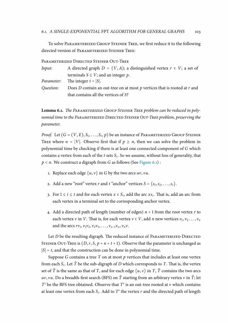
6.1. A SINGLE-EXPONENTIAL FPT ALGORITHM FOR GENERAL GRAPHS 103
To solve Parameterized Group Steiner Tree, we rst reduce it to the following
directed version of Parameterized Steiner Tree:
Parameterized Directed Steiner Out-Tree
Input: A directed graph D = (V ,A); a distinguished vertex r ∈ V ; a set of
terminals S ⊆ V ; and an integer p.
Parameter: e integer t = ∣S∣.
Question: Does D contain an out-tree on at most p vertices that is rooted at r and
that contains all the vertices of S?
Lemma 6.1. e Parameterized Group Steiner Tree problem can be reduced in poly-
nomial time to the ParameterizedDirected SteinerOut-Tree problem, preserving the
parameter.
Proof. Let (G = (V , E), S1, . . . , St , p) be an instance of Parameterized Group Steiner
Tree where n = ∣V ∣. Observe rst that if p ≥ n, then we can solve the problem in
polynomial time by checking if there is at least one connected component of G which
contains a vertex from each of the t sets Si . So we assume, without loss of generality, that
p < n. We construct a digraph from G as follows (See Figure 6.1) :
1. Replace each edge u, v in G by the two arcs uv , vu.
2. Add a new “root” vertex r and t “anchor” vertices S = s1, s2, . . . , st.
3. For 1 ≤ i ≤ t and for each vertex x ∈ Si , add the arc xsi .at is, add an arc from
each vertex in a terminal set to the corresponding anchor vertex.
4. Add a directed path of length (number of edges) n + 1 from the root vertex r to
each vertex v in V .at is, for each vertex v ∈ V , add n new vertices v1, v2 . . . , vn
and the arcs rv1, v1v2, v2v3, . . . , vn−1vn , vnv.
Let D be the resulting digraph.e reduced instance of Parameterized Directed
SteinerOut-Tree is (D, r, S , p + n + t + 1). Observe that the parameter is unchanged as
∣S∣ = t, and that the construction can be done in polynomial time.
Suppose G contains a tree T on at most p vertices that includes at least one vertex
from each Si . Let T be the sub-digraph of D which corresponds to T .at is, the vertex
set of T is the same as that of T , and for each edge u, v in T , T contains the two arcs
uv , vu. Do a breadth-rst search (BFS) on T starting from an arbitrary vertex v in T ; let
T ′ be the BFS tree obtained. Observe that T ′ is an out-tree rooted at v which contains
at least one vertex from each Si . Add to T ′ the vertex r and the directed path of length
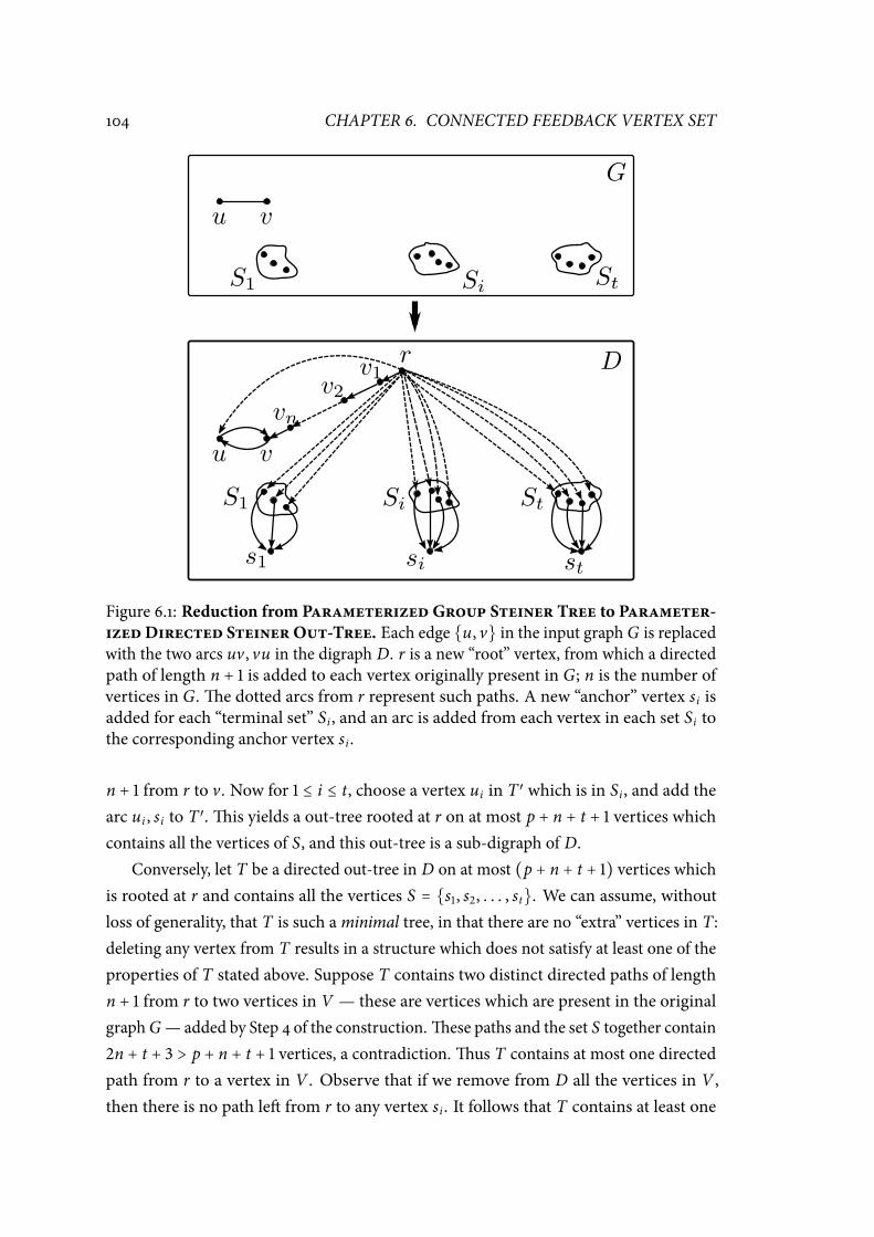
104 CHAPTER 6. CONNECTED FEEDBACK VERTEX SET
Figure 6.1: Reduction from ParameterizedGroup Steiner Tree to Parameter-izedDirected SteinerOut-Tree. Each edge u, v in the input graph G is replacedwith the two arcs uv , vu in the digraph D. r is a new “root” vertex, from which a directed
path of length n + 1 is added to each vertex originally present in G; n is the number of
vertices in G.e dotted arcs from r represent such paths. A new “anchor” vertex si is
added for each “terminal set” Si , and an arc is added from each vertex in each set Si to
the corresponding anchor vertex si .
n + 1 from r to v. Now for 1 ≤ i ≤ t, choose a vertex ui in T ′ which is in Si , and add the
arc ui , si to T ′.is yields a out-tree rooted at r on at most p + n + t + 1 vertices which
contains all the vertices of S, and this out-tree is a sub-digraph of D.
Conversely, let T be a directed out-tree in D on at most (p + n + t + 1) vertices which
is rooted at r and contains all the vertices S = s1, s2, . . . , st. We can assume, without
loss of generality, that T is such aminimal tree, in that there are no “extra” vertices in T :
deleting any vertex from T results in a structure which does not satisfy at least one of the
properties of T stated above. Suppose T contains two distinct directed paths of length
n + 1 from r to two vertices in V — these are vertices which are present in the original
graphG—added by Step 4 of the construction.ese paths and the set S together contain
2n + t + 3 > p + n + t + 1 vertices, a contradiction.us T contains at most one directed
path from r to a vertex in V . Observe that if we remove from D all the vertices in V ,
then there is no path le from r to any vertex si . It follows that T contains at least one
6.1. A SINGLE-EXPONENTIAL FPT ALGORITHM FOR GENERAL GRAPHS 105
directed path from r to some vertex in V .us T contains exactly one directed path, say
r, v1, v2, . . . , vn , v, from r to some vertex v in V .
Suppose there is a vertex u1 ≠ v1 such that r, u1 is an arc in T . Since no vertex in V is
reachable from u1 in T , the subtree of T rooted at u1 can be deleted from T to obtain a
sub-digraph of T which satises all the properties of T stated above.is contradicts the
minimality of T , and so the vertex r has degree exactly 1 in T .
is implies that deleting the vertices r, v1, v2, . . . , vn from T results in a directed
out-tree T on p + t vertices which is rooted at v and contains all of S. Since no vertex
si ∈ S has an arc going out from it, every si is a leaf node in T .erefore, deleting all the
vertices of S from T yields a directed out-tree T ′ on p vertices which is rooted at v and
contains at least one vertex from each set Si .e corresponding tree in G—which has
the same vertex set as T ′, and has an edge in the place of each arc in T ′— is a tree in G
on at most p vertices that includes at least one vertex from each Si .
We now show that Parameterized Directed Steiner Out-Tree can be solved
in 2t ⋅ nO(1) time and polynomial space. Our algorithm for Parameterized Directed
Steiner Out-Tree is modelled aer Nederlof ’s algorithm [94] for Parameterized
Steiner Tree.
First, recall the well-known Inclusion-Exclusion formula [73, Section 1.6]: Let U be
a nite universe, A1, . . . ,At ⊆ U , Ai ≡ U ∖ Ai , and dene ⋂i∈∅ Ai to be the universe U .
en
∣t
⋂i=1
Ai∣ = ∑X⊆[t]
(−1)∣X∣ ∣⋂i∈X
Ai ∣ (6.1)
Given a problem, suppose we dene the sets Ai in such a way that the value of ∣⋂ti=1 Ai ∣
gives us the solution to the problem. One consequence of the above formula is that if, for
each X ⊆ [t],
1. we can evaluate ∣⋂i∈X Ai ∣ in time polynomial in the input size n, and,
2. the size of the universe U can be expressed using polynomially many bits in the
input size n,
thenwe can evaluate ∣⋂ti=1 Ai ∣ in timeO(2t ⋅nO(1)) using space polynomial in n. Essentially,
we evaluate one by one the 2t expressions ∣⋂i∈X Ai ∣— one for each subset of [t]— and
keep a running “signed” sum of their values according to Equation 6.1. From the second
condition above, we need only polynomially many bits in n to store these intermediate
sums.is is the strategy we follow to solve Parameterized Directed Steiner Out-
Tree.
106 CHAPTER 6. CONNECTED FEEDBACK VERTEX SET
Let G ,H be two digraphs. A digraph homomorphism∗ from G to H is a mapping
f ∶ V(G)→ V(H) such that uv ∈ A(G) Ô⇒ f (u) f (v) ∈ A(H). Given a directed graph
D = (V ,A), we dene a directed branching walk B in D to be a pair (TB = (VB ,AB), ϕ),
where TB is an out-tree and ϕ ∶ VB → V is a digraph homomorphism from TB to D. Note
that TB is an arbitrary out-tree, and is not necessarily a subgraph of D.e length of the
directed branching walk B, denoted ∣B∣, is dened to be ∣AB∣. For a node s ∈ V , we say
that the directed branching walk B is from s if ϕ maps the root of TB to s. We dene
ϕ(VB) = ϕ(u) ∣ u ∈ VB and ϕ(AB) = ϕ(a)ϕ(b) ∣ (a, b) ∈ AB.
It turns out that directed branching walks and out-trees stand or fall together.
Claim 1. Let (D, r, S , p) be an instance of the Parameterized Directed Steiner Out-
Tree problem.en there exists an out-tree T = (V ′,A′) in D rooted at r such that S ⊆ V ′
and ∣V ′∣ ≤ p if and only if there exists a directed branching walk B = (TB = (VB ,AB), ϕ) in
D from r such that S ⊆ ϕ(VB) and ∣B∣ ≤ p − 1.
Proof. If T = (V ′,A′) is an out-tree in D rooted at r such that S ⊆ V ′ and ∣V ′∣ ≤ p, then
let (VB ,AB) = TB = T = (V ′,A′), and let ϕ be the identity map on the vertex set VB = V ′
of TB.en ϕ is a digraph homomorphism from TB to D which maps the root r of TB to
the vertex r, S ⊆ ϕ(VB) = VB = V ′, and ∣AB∣ = ∣VB∣−1 ≤ p−1.us B = (TB = (VB ,AB), ϕ)
is a directed branching walk in D from r such that S ⊆ ϕ(VB) and ∣B∣ ≤ p − 1.
Conversely, let B = (TB = (VB ,AB), ϕ) be a directed branching walk in D from r such
that S ⊆ ϕ(VB) and ∣B∣ ≤ p− 1. Mark the vertex r in D. Starting from the root rB of TB, do
a breadth-rst traversal of TB, respecting the directions of the arcs. For each new arc uv
of TB encountered in this traversal, if ϕ(v) is not already marked, then
• Mark the vertex ϕ(v), and
• Mark the arc ϕ(u)ϕ(v).
Let T = (V ′,A′) be the marked sub-digraph of D obtained by this process. Observe
that V ′ = ϕ(VB), and so S ⊆ V ′. Since a vertex in D is marked at most once, T has no
cycles. Note that each time a new vertex is marked, an arc to that vertex from some
previously marked vertex is also marked. It follows that the digraph T is connected, and
is an out-tree rooted at r. Since each arc in AB corresponds to at most one new vertex in
T , and every vertex in T except the root vertex rB corresponds to an arc in AB, it follows
that ∣V ′∣ ≤ 1 + ∣AB∣ ≤ p.us T = (V ′,A′) is an out-tree in D rooted at r such that S ⊆ V ′
and ∣V ′∣ ≤ p.
∗ See the book by Hell and Nešetřil [70] for a detailed treatment of graph homomorphisms.
6.1. A SINGLE-EXPONENTIAL FPT ALGORITHM FOR GENERAL GRAPHS 107
We take advantage of this relation between directed branching walks and rooted
out-trees to solve the Parameterized Directed Steiner Out-Tree problem.e idea
is to count the directed branching walks from a vertex instead of looking for the existence
of an out-tree rooted at that vertex. As we see below, directed branching walks turn out to
be easy to count using the Inclusion-Exclusion formula. Note that we are not interested
in this count per se, but only in whether the count is zero or not. If the count is zero, then
— by Claim 1 — there is no out-tree of the required kind in the digraph, and otherwise
there is.
Let (D = (V ,A), r, S , p) be an instance of the Parameterized Directed Steiner
Out-Tree problem. We now express, as an Inclusion-Exclusion formula, the number
of directed branching walks in D from r such that S ⊆ ϕ(VB) and ∣B∣ ≤ p − 1. Let U be
the set of all directed branching walks from r of length p − 1. For each v ∈ S, let Bv be the
set of all elements of U that contain v.en Bv is the set of all elements of U which do
not contain v, and ⋂v∈S Bv is the set of all directed branching walks that contain all the
vertices of S. Substituting the sets Bv ; v ∈ S in Equation 6.1 we get
∣⋂v∈S
Bv∣ = ∑X⊆S
(−1)∣X∣ ∣⋂u∈X
Bu ∣ (6.2)
By Claim 1, ∣⋂v∈S Bv ∣ > 0 if and only if (D = (V ,A), r, S , p) is a Yes instance.
For X ⊆ S dene X′ = X∪(V ∖S), and let bXj (r) be the number of directed branching
walks from r of length j in the graph D[X′]. Note that⋂u∈X Bu is the set of all elements of
U which do not contain any vertex in X.at is,⋂u∈X Bu is the set of all directed branching
walks from r of length p − 1 in the graph D[(V ∖ X)]. Further, bS∖Xp−1 (r) is the number
of directed branching walks from r of length p − 1 in the graph D[(S ∖ X) ∪ (V ∖ S)] =
D[V ∖ X].us ∣⋂u∈X Bu∣ = bS∖Xp−1 (r).
Let Y be an arbitrary subset of S.e number of directed branching walks of length 0
rooted at r is 1 : the tree TB = (VB ,AB) in this case consists of just a single vertex, and the
homomorphism ϕmaps this vertex to r.us bY0 (r) = 1. Any directed branching walk
(TB = (VB ,AB), ϕ) of length j > 0 rooted at rmaps some vertex inVB to an out-neighbour
s of r in D, and can be split into two parts: a directed branching walk (T1, ϕ1) of length
j′ ≥ 0 rooted at s, and another directed branching walk (T2, ϕ2) of length j − j′ − 1 rooted
at r. e “loss” of 1 corresponds to the arc from r to s present in ϕ(AB). Conversely,
every pair of two such directed branching walks corresponds to a directed branching
walk (TB , ϕ) of length j rooted at r: the tree TB is obtained by adding an arc from the
108 CHAPTER 6. CONNECTED FEEDBACK VERTEX SET
root of T2 to the root of T1, and the homomorphism ϕ is the disjoint union of the two
homomorphisms ϕ1, ϕ2.
It follows that for any j ≥ 0,Y ⊆ S, the number bYj (r) can be computed in time
polynomial in n and j by a simple dynamic programming algorithmbased on the following
recurrence:
bYj (r) =
⎧⎪⎪⎪⎨⎪⎪⎪⎩
1 if j = 0;
∑s∈N+(r)∩Y
∑j1+ j2= j−1
bYj1(s) ⋅ bYj2(r) otherwise.
We now compute ∣⋂v∈S Bv ∣ as per Equation 6.2, by computing successive partial sums
in the expression on the right hand side of this equation. Since ∣⋂v∈X Bv ∣ = bS∖Xp−1 (r) for
each X ⊆ S, to compute the value ∣⋂v∈X Bv ∣ ;X ⊆ S it is sucient to compute bS∖Xp−1 (r)
instead. To compute each partial sum of the right hand side of Equation 6.2, our algorithm
computes the next value bYp−1(r) needed and adds (or subtracts, as the case may be) it to
(or from) the partial sum computed so far. Since there are 2∣S∣ = 2t values to be computed
and each value can be computed in polynomial time, this can be done in 2t ⋅ nO(1) time.
e incremental process described above takes only polynomial space, since only the
partial sum is stored between computations. We return Yes if the nal value is larger than
zero, and No otherwise.us we have shown that
Lemma 6.2. e Parameterized Directed Steiner Out-Tree problem can be solved
in 2t ⋅ nO(1) time using polynomial space.
Lemma 6.1 and Lemma 6.2 together imply:
Lemma 6.3. e Parameterized Group Steiner Tree problem can be solved in (2t ⋅
nO(1)) time using polynomial space.
6.1.2 Compact Representations of Feedback Vertex Sets
A second ingredient in our FPT algorithm for Parameterized Connected Feedback
Vertex Set is an algorithmwhich takes a graphG as input and enumerates “essentially all”
minimal feedback vertex sets of G of size at most k inO⋆(ck) time for a constant c. Recall
from the Introduction that one cannot hope, in general, to enumerate allminimal feedback
vertex sets of size at most k of a graph in f (k) time for any function f . For example, a
graph which is a collection of k vertex-disjoint cycles, each of length approximately n/k,
has Ω(( nk)k)minimal feedback vertex sets, each obtained by choosing one vertex from
each cycle.
6.1. A SINGLE-EXPONENTIAL FPT ALGORITHM FOR GENERAL GRAPHS 109
A way around this problem was found by Guo et al. [64], who introduced the notion
of compact representations of feedback vertex sets. In the context of feedback vertex sets,
a compact representation of a graph G = (V , E) is a set C of pairwise disjoint subsets of V
such that choosing exactly one vertex from every set in C results in a minimal feedback
set for G. A compact representation is called a k-compact representation if the number of
sets in the representation is at most k. It follows directly from this denition that for each
connected feedback vertex set S of size at most k, there exists a minimal feedback vertex
set S′ ⊆ S and some k-compact representation C such that we can obtain S′ by picking
one vertex from each set in C.
Guo et al. showed that given a graph G and a number k, one can enumerate all
k-compact representations of G in O⋆(ck) time for some constant c.
eorem 6.1. [64, eorem 7] Given a graph G and a positive integer k as input, all k-
compact representations of G can be enumerated in O(ck ⋅ ∣G∣) time where c is a constant.
e constant c implied by the proof of this theorem is more than 160. is can be
signicantly improved using a result from the recent work of Cao et al. [22] where the
authors present the current fastest deterministic FPT algorithm for Parameterized
Feedback Vertex Set. We now sketch how this is accomplished. Both Guo et al. and
Cao et al. use the following problem on the way to obtaining their respective results; our
denition matches that of Cao et al:
Parameterized Forest Bipartition
Input: An undirected graph G = (V , E), possibly with multiple edges and loops,
and a set S ⊆ V such that ∣S∣ = k + 1 and G ∖ S is acyclic.
Parameter: e integer k.
Question: Does G have a feedback vertex set of size at most k which is contained in
V ∖ S?
Cao et al. describe a set of reduction rules such that if a Yes instance of the Paramet-
erized Forest Bipartition problem is reduced with respect to this set of rules, then
the instance has size at most 4k + 1. In particular, in such a reduced instance we have
∣V ∖ S∣ ≤ 3k. Guo et al. bound the number of k-compact representations by
∑k
i=0(k + 1
i)(∑
k−i
j=0(X
j)(
Y
k − i − j)) ,
110 CHAPTER 6. CONNECTED FEEDBACK VERTEX SET
where X is the number of vertices in V ∖ S that have degree at least three in G, and Y
is the number of paths in G[V ∖ S] whose endpoints are vertices of degree at least three
and internal vertices have degree exactly two in G.
Suppose the instance (G , k) of Parameterized ForestBipartition is a Yes instance,
and has a feedback vertex set of size at most r ≤ k which is contained in V ∖ S. e
reduction rules described by Cao et al. imply that in such a case, the reduced instance has
∣X∣ ≤ 3r. Further, Guo et al. show that ∣Y ∣ ≤ ∣X∣+2r. Using these bounds in the arguments
of Guo et al., we get that the number of k-compact representations is at most
k
∑i=0
(k + 1
i)⎛
⎝
k−i
∑j=0
(3(k + 1 − i)
j)(5(k + 1 − i)
k − i − j)⎞
⎠≤
k
∑i=0
(k + 1
i)(8(k + 1 − i)
k − i) =
k
∑i=0
(9k − 8i + 9
k) ≤
k(9k + 9
k)
is expression is upper bounded by 23.1k+1 ⋅ k. Guo et al. show that all these repres-
entations can be enumerated with O(∣E(G)∣) delay, and so we have
eorem 6.2. Given a graph G = (V , E) and an integer k, all the k-compact representa-
tions of G can be enumerated in O(23.1k ⋅ k∣E∣) time.
In contrast, the constant at the base of the expression for the running time in Guo et
al.’s result —eorem 6.1 — is more than 160, because the best bound known for ∣X∣ at
that time was 14k.
6.1.3 An FPT Algorithm for PARAMETERIZED CONNECTED FEEDBACK
VERTEX SET
Recall that the Parameterized Connected Feedback Vertex Set problem is dened
as follows
Parameterized Connected Feedback Vertex Set
Input: An undirected graph G = (V , E), and a positive integer k.
Parameter: e integer k.
Question: Does there exist a set S ⊆ V of at most k vertices of G such that (i) the
graph G[V ∖ S] has no cycles, and (ii) the graph G[S] is connected?
6.2. A FASTER FPT ALGORITHM FOR H-MINOR FREE GRAPHS 111
Given the two FPT algorithms of the previous subsections — one for Parameterized
Group Steiner Tree and the other for enumerating all k-compact representations— it is
straightforward to derive an FPT algorithm for Parameterized Connected Feedback
Vertex Set.is algorithm enumerates all k-compact representations of the input graph.
For each such representation C = S1, S2, . . . , Sr; 1 ≤ r ≤ k, the algorithm solves the
Parameterized Group Steiner Tree problem on the input (G; S1, S2, . . . , Sr; k). If
the answer to this latter problem is No for every k-compact representation, then the
algorithm returns No : the graphG has no connected feedback vertex set of size at most k.
Otherwise, it returns the rst (group) Steiner tree found by the Parameterized Group
Steiner Tree algorithm.e correctness of this procedure is evident from the discussion
at the beginning of this subsection, and so from Lemma 6.3 andeorem 6.2 we get
eorem 6.3. e Parameterized Connected Feedback Vertex Set problem is xed-
parameter tractable. Given a graph G = (V , E) and an integer k, one can decide whether
G has a connected feedback set of size at most k in 46.2k ⋅ nO(1) time.
6.2 A Faster FPT Algorithm for H-minor free Graphs
In this section we show that for any xed graph H, the Parameterized Connected
Feedback Vertex Set problem can be solved in 2O(
√
k log k)nO(1) time on the class of
H-minor-free graphs.is running time is achieved by doing dynamic programming
(DP) on a tree decomposition of the input graph of suitably bounded tree width. See
Chapter 2 for the denitions of the various terms used in this section. We briey recall
the notion of a nice tree decomposition which is crucial in describing the DP algorithm.
A tree decomposition (T = (VT , ET),X = Xtt∈VT) of a graph G = (V , E) is called a
nice tree decomposition [14] if the following conditions are satised:
• Every node of the tree T has at most two children. A node that has no children is
called a leaf node.e non-leaf nodes are of three kinds:
– If a node t has two children t1 and t2, then Xt = Xt1 = Xt2 , and t is called a
join node.
– if a node t has one child t1, then either ∣Xt ∣ = ∣Xt1 ∣ + 1 and Xt1 ⊂ Xt (t is called
an introduce node), or ∣Xt ∣ = ∣Xt1 ∣ − 1 and Xt ⊂ Xt1 (t is called a forget node).

112 CHAPTER 6. CONNECTED FEEDBACK VERTEX SET
It is possible to transform a given tree decomposition into a nice tree decomposition of
the same width in time O(∣V ∣ + ∣E∣) [14].
is section is divided into two subsections. In the rst subsection we show that Para-
meterized Connected Feedback Vertex Set can be solved in time O(wO(w)nO(1)) on
graphs with treewidth bounded by w. In the second subsection we bound the treewidth
of the input graph by O(√k) using well-known “grid theorems”. Together, these yield an
algorithm with a running time of the stated kind.
6.2.1 CONNECTED FEEDBACK VERTEX SET Parameterized by Treewidth
In this section we show that the minimization version of the Connected Feedback
Vertex Set problem is FPT when the treewidth of the input graph is the parameter.at
is, we show that the following problem is FPT:
Input: An undirected graph G = (V , E); an integer k; and a nice tree decompos-
ition of G of width w.
Parameter: e treewidth w of the graph G.
Question: Find a set S ⊆ V such that G ∖ S is acyclic, G[S] is connected, and for any
connected feedback vertex set R of G, ∣S∣ ≤ ∣R∣.
For this problem, we design a dynamic programming algorithm on the nice tree
decomposition which runs in time wO(w) ⋅ nO(1). See, for example, Hannes Moser’s
Master’s thesis [92] for a detailed exposition of this algorithmic paradigm; in particular,
our algorithm for Connected Feedback Vertex Set is similar in spirit to the algorithm
given by Moser for the Connected Vertex Cover problem. We start by giving an
intuitive overview of the algorithm.
e general strategy used to obtain FPT — with the parameter being the treewidth —
algorithms by dynamic programming on nice tree decompositions is to design a dynamic
programming table (DP table) for each node of the nice tree decomposition such that:
1. e DP table for a leaf node can be computed in time which is FPT in the treewidth
— that is, of the form f (w) ⋅nO(1) wherew is the treewidth, n the number of vertices
in the graph, and f a computable function;
2. Starting at the leaves and going up to the root, given the DP table(s) of the child(ren)
node(s) of a given node, the DP table for this node can be computed in time FPT
in the treewidth; and,
6.2. A FASTER FPT ALGORITHM FOR H-MINOR FREE GRAPHS 113
3. e desired answer can be computed in FPT time (in many cases, read o directly)
from the DP table for the root node.
One fruitful approach towards designing the DP table for solving “subset problems”
(where the task is to nd a subset of vertices which has some specied property) is to
look at how a solution intersects the subgraph induced by all the vertices in a subtree
rooted at an arbitrary node in the tree decomposition. Observe that any solution must
intersect such a subgraph in some manner; the DP table must account for all possible
ways in which this can happen, and must be designed in such a way that it is easy (in the
sense listed above) to update.
For Connected Feedback Vertex Set, it turns out that a correct way to design
the DP table is to try to capture the connectivity properties of a partial solution when
restricted to the subgraphs induced by subtrees of the tree decomposition. To be more
precise: Let F be some xed connected feedback vertex set of the input graph G = (V , E)
of size at most k, and let Gi be the subgraph induced by the vertices in the subtree rooted
at an arbitrary node i in a nice tree decomposition of G. G[F] restricted to the set Xi
is, in general, a disconnected graph. So is the forest G[V ∖ F] restricted to the set Xi .
Our dynamic programming algorithm tries to guess the components of each of the two
subgraphsG[F ∩Xi] andG[(V ∖F)∩Xi]; it turns out that with this information in hand,
it is not dicult to compute the DP tables of the nodes at the next higher level in the tree
decomposition, be it an introduce, forget, or join node; the details follow.
Let (T = (I, F) , Xi ∣i ∈ I) be a nice tree decomposition of the input graph G of
width w and rooted at r ∈ I. We let Ti denote the subtree of T rooted at i ∈ I, and use
Gi = (Vi , Ei) to denote the subgraph of G induced on all the vertices of G in the subtree
Ti , that is, Gi = G[⋃ j∈V(Ti)X j].
For each node i ∈ I we compute a table Ai , the rows of which are 4-tuples [S , P,Y , val].
Table Ai contains one row for each combination of the rst three components which
denote the following:
• S is a subset of Xi .
• P is a partition of S into at most ∣S∣ labelled pieces.
• Y is a partition of Xi ∖ S into at most ∣Xi ∖ S∣ labelled pieces.
We use P(v) (resp. Y(v)) to denote the piece of the partition P (resp. Y) that contains
the vertex v. We let ∣P∣ (resp. ∣Y ∣) denote the number of pieces in the partition P (resp.
Y).e last component val, also denoted as Ai [S , P,Y], is the size of a smallest feedback
vertex set Fi ⊆ V (Gi) of Gi which satises the following properties:
114 CHAPTER 6. CONNECTED FEEDBACK VERTEX SET
• If S = ∅, then Fi is connected in Gi .
• If S ≠ ∅, then
– Fi ∩ Xi = S.
– All vertices of S that are in any one piece of P are in a single connectedcomponent ofGi[Fi]. MoreoverGi[Fi] has exactly ∣P∣ connected components.
– All vertices of Xi ∖ S that are in the same piece of Y are in a single connected
component (a tree) of Gi[Vi ∖ Fi]. Moreover Gi[Vi ∖ Fi] has at least ∣Y ∣
connected components.
We say that a feedback vertex set Fi which satises the above conditions is feasible
for the triple (S , P,Y).
If there is no such set Fi , then the last component of the row is set to∞.
We x an arbitrary ordering of the vertices of Xi , and compute the table Ai for each
node i ∈ I of the tree decomposition. Since there are at most w + 1 vertices in each bag Xi ,
there are no more than
w+1
∑i=0
(w + 1
i)i i ⋅ (w + 1 − i)
w+1−i≤ (2w + 2)
2w+2(6.3)
rows in any table Ai . We compute the tables Ai starting from the leaf nodes of the tree
decomposition and going up to the root.
Leaf Nodes. Let i be a leaf node of the tree decomposition. We compute the table Ai as
follows. For each triple (S , P,Y) where S is a subset of Xi , P a partition of S, and
Y a partition of Xi ∖ S:
• Set Ai [S , P,Y] =∞ if at least one of the following holds:
– Gi ∖ S contains a cycle (i.e., S is not a feedback vertex set of Gi).
– At least one piece of P is not connected in Gi[S] or if Gi[S] has less than
∣S∣ connected components.
– At least one piece of Y is not connected in Gi[Vi ∖ S] or if Gi[Vi ∖ S] has
less than ∣Y ∣ connected components.
• In all other cases, set Ai [S , P,Y] = ∣S∣.
It is easy to see that this computation correctly determines the last component of
each row of Ai for a leaf node i of the tree decomposition.
6.2. A FASTER FPT ALGORITHM FOR H-MINOR FREE GRAPHS 115
Introduce Nodes. Let i be an introduce node and j its unique child. Let x ∈ Xi ∖ X j be
the introduced vertex. For each triple (S , P,Y), we compute the entry Ai[S , P,Y]
as follows.
Case 1. x ∈ S. If N(x) ∩ S ⊊ P(x), then set Ai[S , P,Y] =∞. Otherwise, if S = x
and 0 < A j[∅, P,Y] <∞, then set Ai[S , P,Y] =∞. Otherwise,
• Subcase 1. P(x) = x. Set Ai[S , P,Y] = A j[S ∖ x, P ∖ P(x),Y] + 1.
• Subcase 2: ∣P(x)∣ ≥ 2 and N(x) ∩ P(x) = ∅. Set Ai[S , P,Y] = ∞, as no
extension of S to an fvs for Gi can make P(x) connected.
• Subcase 3: ∣P(x)∣ ≥ 2 and N(x) ∩ P(x) ≠ ∅. Let A be the set of all rows
[S′, P′,Y] of the table A j that satisfy the following conditions:
– S′ = S ∖ x.
– P′ = (P ∖P(x))∪Q, where Q is a partition of P(x)∖x such that each
piece of Q contains an element of N(x) ∩ P(x).
Set Ai[S , P,Y] =min[S′ ,P′ ,Y]∈AA j[S′, P′,Y] + 1.
To illustrate how the correctness of the dierent cases can be established, we now
describe why the computation of Ai[S , P,Y] in Subcase 1 is correct. Let Fi be a
feedback vertex set of Gi . If all vertices of S that are in any one piece of P are in
a single connected component of Gi[Fi], and N(x) ∩ S ⊊ P(x), then the number
of connected components of Gi[Fi] is strictly less than ∣P∣. is justies setting
Ai[S , P,Y] to∞ in this case. If S = x and Fi is feasible for (S , P,Y), then Fi can
have no vertex in G j. If 0 < A j[∅, P,Y] <∞, then there are cycles in G j, and this
justies setting Ai[S , P,Y] to∞ in this case.
Now we consider Subcase 1. In this case the graph Gi can be obtained from the
graph G j by adding the vertex x and zero or more edges from x to vertices in
Xi ∖ S = X j ∖ S. Let F ′j = Fi ∖ x, S′ = S ∖ x. Let P′ be the natural restriction
of P to S′. It is not dicult to see that (1) F ′j is a feedback vertex set of G j, and,
(2) if Fi is feasible for (S , P,Y), then F ′j is feasible for (S′, P′,Y). Conversely, if
F j is a nonempty feedback vertex set of G j and F j is feasible for (S′, P′,Y), then
F ′i = F j ∪ x is a feedback vertex set of Gi which is feasible for (S , P,Y). Since
∣S∣ = ∣S′∣ + 1, this justies Subcase 1.
e correctness of the remaining cases can be argued in a similar fashion.
Case 2. x ∉ S. If N(x) ∩ (Xi ∖ S) ⊊ Y(x), then set Ai[S , P,Y] =∞. Otherwise,

116 CHAPTER 6. CONNECTED FEEDBACK VERTEX SET
• Subcase 1: Y(x) = x. Set Ai[S , P,Y] = A j[S , P,Y ∖ Y(x)].
• Subcase 2: ∣Y(x)∣ ≥ 2 and N(x) ∩ Y(x) = ∅. Set Ai[S , P,Y] = ∞, as no
extension of S to an fvs Fi for Gi can make Y(x) a connected component in
Gi[Vi ∖ Fi].
• Subcase 3: ∣Y(x)∣ ≥ 2 and N(x) ∩ Y(x) ≠ ∅. Let A be the set of all rows
[S , P,Y ′] of the table A j where Y ′ = (Y ∖ Y(x)) ∪ Q, and Q is a partition
of Y(x) ∖ x such that each piece of Q contains exactly one element of
N(x) ∩ Y(x). Set Ai[S , P,Y] =min[S ,P,Y ′]∈AA j[S , P,Y ′].
Forget Nodes. Let i be a forget node and j its unique child node. Let x ∈ X j ∖ Xi be the
forgotten vertex. For each triple (S , P,Y) in the table Ai , letA be the set of all rows
[S′, P′,Y] of the table A j that satisfy the following conditions:
• S′ = S ∪ x, and
• P′(x) = P(y) ∪ x for some y ∈ S.
LetB be the set of all rows [S , P,Y ′] of the table A j such that Y ′(x) = Y(z) ∪ x
for some z ∈ S. Set
Ai[S , P,Y] =min min[S′ ,P′ ,Y]∈A
A j[S′, P′,Y], min
[S ,P,Y ′]∈BA j[S , P,Y
′] .
Join Nodes. Let i be a join node and j and l its children. For each triple (S , P,Y) we
compute Ai[S , P,Y] as follows.
• Case 1. S = ∅. If both A j[∅, P,Y] and Al[∅, P,Y] are positive nite, then set
Ai[∅, P,Y] =∞. Else set Ai[∅, P,Y] =maxA j[∅, P,Y],Al[∅, P,Y].
• Case 2. S ≠ ∅. LetAdenote the set of all pairs of triples ⟨(S , P1,Y1), (S , P2,Y2)⟩,
where (S , P1,Y1) ∈ A j and (S , P2,Y2) ∈ Al with the following property: Start-
ing with the partitions Qp = P1 and Qy = Y1 and repeatedly applying the
following set of operations, we reach stable partitions that are identical to P
and Y .e rst operation that we apply is:
If there exist vertices u, v ∈ S such that they are in dierent pieces
of Qp but are in the same piece of P2, delete Qp(u) and Qp(v) from
Qp and add Qp(u) ∪ Qp(v).
To describe the second set of operations, we need somenotation. Let Z = Xi∖S
and let the connected components of Gi[Z] be C1, . . . ,Cq. First contract each
connected component Ci to a vertex ci , the representative of that component,
6.2. A FASTER FPT ALGORITHM FOR H-MINOR FREE GRAPHS 117
and let C = c1, . . . , cq. Note that for each 1 ≤ i ≤ q, the component Ci is
not split across pieces in either Y1 or Y2. Denote by Y′
1 and Y′
2 the partitions
obtained from Y1 and Y2, respectively, be replacing each connected component
Ci by its representative vertex ci . Let Qy = Y ′
1 . Repeat until no longer possible:
If there exist ca , cb ∈ C that are in dierent pieces of Qy but in
the same piece of Y2 then delete Qy(ca),Qy(cb) from Qy and add
Qy(ca) ∪ Qy(cb) provided the following condition holds: for all
ce ∈ C ∖ ca , cb either Y2(ce) ∩Qy(ca) = ∅ or Y2(ce) ∩Qy(cb) = ∅.
If this latter condition does not hold, move on to the next pair of triples.
Finally expand each ci to the connected component it represents.
Set
Ai[S , P,Y] = min⟨(S ,P1 ,Y1),(S ,P2 ,Y2)⟩∈A
A j[S , P1,Y1] + Al[S , P2,Y2] − ∣S∣.
e stated conditions ensure that u, v ∈ S are in the same piece of P if and
only if for each ⟨(S , P1,Y1), (S , P2,Y2)⟩ ∈ A, they are in the same piece of P1 or
of P2 (or both). Similarly, the stated conditions ensure that merging solutions
at join nodes do not create new cycles. Given this, it is easy to verify that the
above computation correctly determines Ai [S , P,Y].
Root Node. We compute the size of a smallest connected feedback vertex set of G fromthe table Ar for the root node r as follows. Find the minimum of Ar[S , P,Y] over
all triples (S , P,Y), where S ⊆ Xr, P a partition of S such that P consists of a single
(possibly empty) piece and Y is a partition of Xr ∖ S.is minimum is the size of a
smallest connected feedback vertex set of G.
is concludes the description of the dynamic programming algorithm for Con-
nected Feedback Vertex Set when the treewidth of the input graph is bounded by w.
From the above description and the size of tables being bounded by (2w + 2)2w+2 (See
Equation 6.3), we obtain
eorem 6.4. Given a graph G = (V , E) and a tree-decomposition of G of width w, one
can compute the size of a smallest connected feedback vertex set of G (if it exists) in (2w +
2)2w+2 ⋅ nO(1) time.
6.2.2 A Sub-Exponential FPT Algorithm for H-Minor Free Graphs
As we describe in this subsection,eorem 6.4 implies that for any xed graph H, the
Parameterized Connected Feedback Vertex Set problem can be solved in sub-
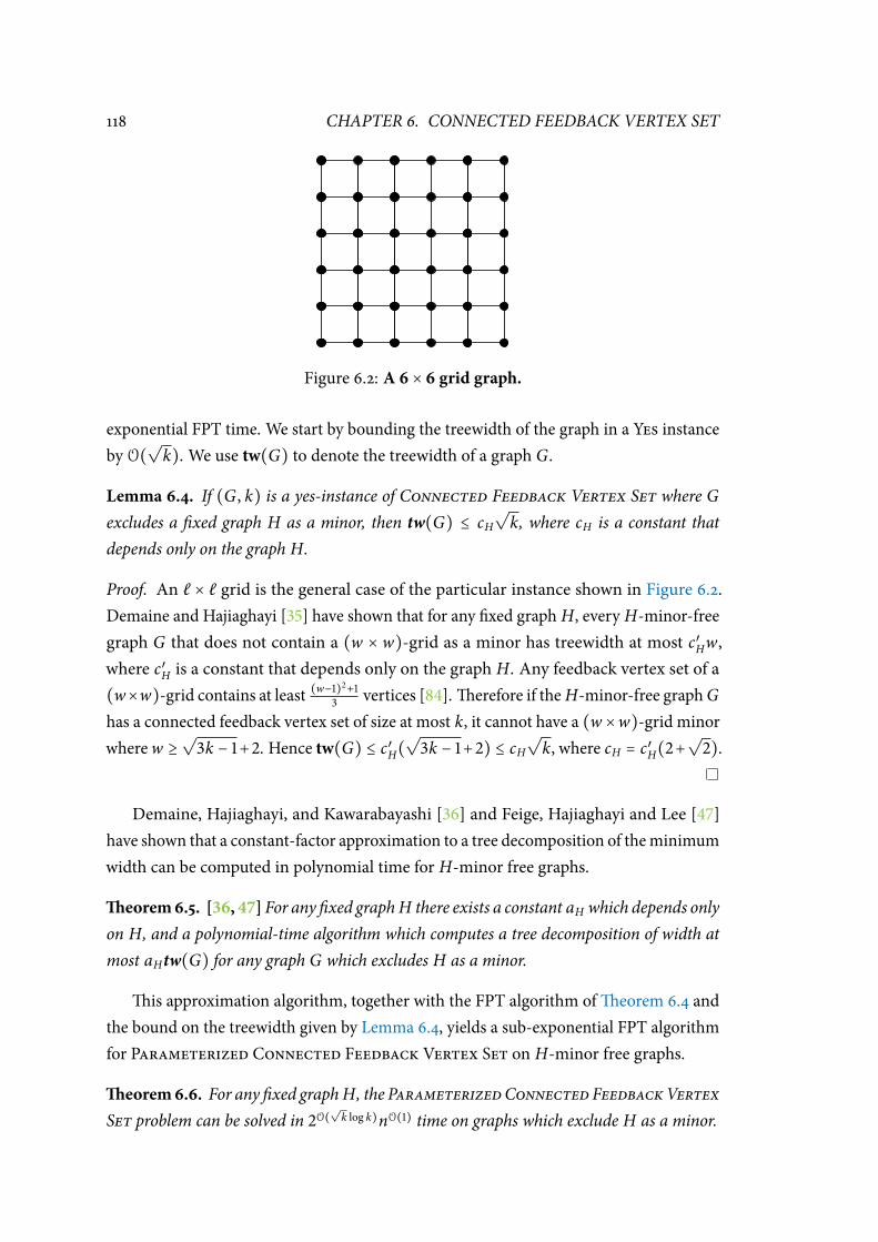
118 CHAPTER 6. CONNECTED FEEDBACK VERTEX SET
Figure 6.2: A 6 × 6 grid graph.
exponential FPT time. We start by bounding the treewidth of the graph in a Yes instance
by O(√k). We use tw(G) to denote the treewidth of a graph G.
Lemma 6.4. If (G , k) is a yes-instance of Connected Feedback Vertex Set where G
excludes a xed graph H as a minor, then tw(G) ≤ cH√k, where cH is a constant that
depends only on the graph H.
Proof. An ℓ × ℓ grid is the general case of the particular instance shown in Figure 6.2.
Demaine and Hajiaghayi [35] have shown that for any xed graph H, every H-minor-free
graph G that does not contain a (w × w)-grid as a minor has treewidth at most c′Hw,
where c′H is a constant that depends only on the graph H. Any feedback vertex set of a
(w×w)-grid contains at least(w−1)2+1
3vertices [84].erefore if theH-minor-free graphG
has a connected feedback vertex set of size at most k, it cannot have a (w ×w)-grid minor
wherew ≥√3k − 1+2. Hence tw(G) ≤ c′H(
√3k − 1+2) ≤ cH
√k, where cH = c′H(2+
√2).
Demaine, Hajiaghayi, and Kawarabayashi [36] and Feige, Hajiaghayi and Lee [47]
have shown that a constant-factor approximation to a tree decomposition of theminimum
width can be computed in polynomial time for H-minor free graphs.
eorem6.5. [36, 47] For any xed graphH there exists a constant aH which depends only
on H, and a polynomial-time algorithm which computes a tree decomposition of width at
most aHtw(G) for any graph G which excludes H as a minor.
is approximation algorithm, together with the FPT algorithm ofeorem 6.4 and
the bound on the treewidth given by Lemma 6.4, yields a sub-exponential FPT algorithm
for Parameterized Connected Feedback Vertex Set on H-minor free graphs.
eorem6.6. For any xed graph H, the ParameterizedConnected FeedbackVertex
Set problem can be solved in 2O(
√
k log k)nO(1) time on graphs which exclude H as a minor.
6.3. KERNELIZATION COMPLEXITY 119
Proof. Let aH , cH be the constants guaranteed to exist for H as pereorem 6.5 and
Lemma 6.4, respectively. Given an instance (G , k) of Parameterized Connected
Feedback Vertex Set where the graph G does not contain H as a minor, we rst nd
an aH-approximate minimum tree-decomposition T of G using the polynomial-time
constant-factor approximation algorithm ofeorem 6.5. If this tree decomposition has
width more than aHcH√k, then byeorem 6.5 tw(G) > cH
√k, and so by Lemma 6.4 G
has no connected feedback vertex set of size at most k. In this case the algorithm returns
No as the answer.
In the other case, T has width at most aHcH√k. Now the algorithm invokes the
dynamic programming algorithm ofeorem 6.4 on the tree decomposition T to nd the
size s of a smallest connected feedback vertex set of G in (2aHcH√k + 2)2aH cH
√
k+2 ⋅ nO(1)
time. If s ≤ k then the algorithm returns Yes. If s > k, or if G has no connected
feedback vertex set, then the algorithm returns No. In the worst case this algorithm
takes (2aHcH√k + 2)2aH cH
√
k+2 ⋅ nO(1) < (c√k)c
√
k ⋅ nO(1) = 2d√
k log k ⋅ nO(1) time where
c = 2aHcH + 1, d =c log c
2.
6.3 Kernelization Complexity
Although Parameterized Connected Feedback Vertex Set is xed-parameter tract-
able, it is unlikely to admit a polynomial kernel, as we show below. Contrast this with the
closely related Parameterized FeedbackVertex Set problemwhich admits a quadratic
kernel [107]. To prove this lower bound, we use notions and results from the recently
developed theory of kernel lower bounds; these are described in detail in Section 2.2.1.
eorem 6.7. e Parameterized Connected Feedback Vertex Set problem does
not admit a polynomial kernel unless the Polynomial Hierarchy (PH) collapses to the third
level.
Proof. We exhibit a polynomial parameter transformation — PPT — from Paramet-
erized Connected Vertex Cover (dened below) to Parameterized Connected
Feedback Vertex Set.
Parameterized Connected Vertex Cover
Input: An undirected graph G = (V , E), and a positive integer k.
Parameter: e integer k.
Question: Does there exist a set S ⊆ V of at most k vertices of G such that (i) the
graph G[V ∖ S] has no edges, and (ii) the graph G[S] is connected?

120 CHAPTER 6. CONNECTED FEEDBACK VERTEX SET
is problemdoes not admit a polynomial kernel unless PH collapses to the third level [39].
e derived classical problem corresponding to Parameterized Connected Vertex
Cover, namely Connected Vertex Cover, is NP-complete even in planar graphs of
maximum degree four [58].e derived classical problem corresponding to Parameter-
izedConnected FeedbackVertex Set, namely Connected FeedbackVertex Set, is
clearly in NP. It follows fromeorem 2.3 that Parameterized Connected Feedback
Vertex Set does not admit a polynomial kernel unless PH collapses to the third level.
We now describe the transformation.
Given an instance (G = (V , E), k) of the Parameterized Connected Vertex
Cover problem, construct a new graph G′ from G′ as follows: For each edge u, v ∈ E,
add a new vertex uv and the edges u, uv, v , uv.is completes the construction of
G′; G′, k is the instance of Parameterized Connected Feedback Vertex Set.
Let S be a connected vertex cover of size at most k in G. Since S is a vertex cover of G,
no edge originally present in G is present in G′ ∖ S.us all edges in any cycle in G′ ∖ S
are “new” edges — those which are added by the construction. Each such new edge is
incident on one “new” vertex, and so any cycle in G′ ∖ S contains at least one new vertex.
For any new vertex uv in G′, at least one of its two neighbours u, v is present in S, or
else the edge u, v is not covered by S.us any new vertex uv has degree at most one
in G′ ∖ S, and so cannot be part of any cycle in G′ ∖ S.
Putting these together, it follows that G′ ∖ S contains no cycles.us S is a feedback
vertex set of G′. Since E(G′) ⊇ E(G) and G[S] is connected, so is G′[S]. us S′ is a
connected feedback vertex set of G′, of size at most k.
Conversely, suppose S is a connected feedback vertex set of G′, of size at most k.
Suppose S contains uv, a newly introduced vertex of degree two. If S = uv, then
S′ = v is also a connected feedback vertex set of G′ of the same size as S, since the
vertex v is present in every cycle which passes through uv. If S ≠ uv, then since G′[S]
is a connected graph, S must contain at least one of the two neighbours u, v of uv. If S
contains both u and v, then S′ = S ∖uv is a smaller connected feedback vertex set of G′,
because (i) any cycle that passes through uv necessarily passes through both u and v, and
(ii) the edge u, v is present in G′. If S contains exactly one of u or v (say u), then for the
same reasons as above, S′ = (S ∖ uv) ∪ v is a connected feedback vertex set of G′.
We may therefore assume, without loss of generality, that the set S contains no newly
introduced vertices; that is, S ⊆ V . Since G′[V] = G, S is connected in G′, and S ⊆ V , it
follows that G[S] is connected. If G[V ∖ S] contains an edge (u, v), then by construction,
G′ ∖ S contains the triangle (u, v , uv), which contradicts the assumption that S is a
feedback vertex set of G′. Hence S is a vertex cover of G.us S is a connected vertex
cover of G, of size at most k.
6.4. CONCLUSION 121
Interestingly, recent meta-theorems on kernelization due to Fomin et al. [56] imply
that Parameterized Connected Feedback Vertex Set has polynomial kernels on any
graph class which excludes a xed apex graph H as a minor.
6.4 Conclusion
In this chapter we described our study of the parameterized complexity of the Connec-
ted Feedback Vertex Set problem, which is a connected variant of the well-studied
FeedbackVertex Set problem. We showed that when parameterized by the size k of the
solution, the problem is xed-parameter tractable (FPT) and can be solved in O⋆(46.2k)
time. On the way to obtaining this result, we showed that two parameterized variants
of the classical Steiner Tree problem, namely Parameterized Directed Steiner
Out-Tree and Parameterized Group Steiner Tree, are FPT when the parameter
is the size t of the number of terminals (respectively, terminal sets) and can be solved
in O⋆(2t) time. We feel that these results could be of use in showing that other con-
nectivity problems are FPT. Very recently, Cygan et al. [30] showed that Parameterized
Connected Feedback Vertex Set can be solved in randomized O⋆(3k) time.
We then investigated the parameterized variant of Connected FeedbackVertex Set
where the parameter is the treewidth w of the input graph. We showed that this problem
is FPT and can be solved in O⋆((2w + 2)2w+2) time. Using this fact and an O(√k) bound
on the treewidth of a Yes instance which follows from an excluded-grid property, we
showed that the Parameterized Connected Feedback Vertex Set problem can be
solved in O⋆(2O(
√
k log k)) time on graphs which exclude some xed graph H as a minor.
Finally, we examined the kernelization complexity of the Parameterized Connec-
ted Feedback Vertex Set problem, and showed that the problem is unlikely to have a
polynomial kernel on graphs in general, in stark contrast to the closely related Paramet-
erized Feedback Vertex Set problem which has a quadratic kernel on general graphs.
We note that some recent meta-theorems on kernelization imply that Parameterized
Connected Feedback Vertex Set has polynomial kernel on any graph class which
excludes a xed apex graph H as a minor.
ere are notmany results known for theConnectedFeedbackVertex Setproblem,
even from the point of view of classical complexity.e only classical results of which we
are aware are for the problem restricted to planar graphs. Bodlaender et al. [16] derive
many positive results for an edge-weighted planar variant of the problem, and Grigoriev
and Sitters [61] derive a constant factor approximation algorithm and a polynomial time
approximation scheme for the unweighted planar variant where the minimum degree is
at least 3.
122 CHAPTER 6. CONNECTED FEEDBACK VERTEX SET
In particular, no non-trivial polynomial-time approximation algorithm is known
for the Connected Feedback Vertex Set problem on general graphs. Note that our
FPT algorithm for the problem suggests a — trivial — polynomial-time approximation
algorithm with approximation factor n/c log n for any constant c, where n is the number
of vertices in the input graph. Aer doing the obvious sanity checks for connectivity, such
an algorithm would run our FPT algorithm for k = 1, , 2, . . . , c log n, each time stopping
aer O⋆(46.2k) steps. is takes nO(1) time. If the FPT algorithm nds a connected
feedback vertex set S of the input graph, then the approximation algorithm returns the
rst such set as an — exact — answer. Otherwise, it returns the vertex set of the input
graph, which is a solution and is no larger than n/c log n times the smallest connected
feedback vertex set.
us an interesting open problem is to nd a polynomial-time approximation al-
gorithm for the Connected Feedback Vertex Set problem with an approximation
ratio asymptotically better than n/ log n, or to show that no such algorithm exists. Another
question which we nd interesting is whether Parameterized Connected Feedback
Vertex Set admits a polynomial kernel on graphs excluding an arbitrary xed graph
H as a minor. It will also be interesting to nd other cases where an application of the
O⋆(2t) algorithm for ParameterizedGroup Steiner Tree/ParameterizedDirected
Steiner Out-Tree yields fast FPT algorithms.
CHAPTER 7
Total Vertex Cover and Total Edge Cover
Given a graph G and a positive integer k as input, the Vertex Cover problem
asks whether G has a set of at most k vertices — a vertex cover of G — such
that every edge of G has at least one of these vertices as an end point.e Edge
Cover problem is quite similar : given (G , k) as input, the question here is whetherG has
a set of at most k edges— an edge cover ofG— such that every vertex inG is an end point
of at least one of these edges. Vertex Cover is a classical NP-hard problem [75] whose
parameterized version with k as the parameter — Parameterized Vertex Cover— is
arguably the most investigated problem in parameterized algorithmics.e fastest known
FPT algorithm for Parameterized Vertex Cover runs in O⋆(1.2738k) time [25], and
the problem has a kernel with at most 2k vertices [23]. In contrast, the Edge Cover
problem is solvable in polynomial time [96].
We investigate the parameterized complexity of variants of Vertex Cover and Edge
Cover where additional connectivity constraints are imposed on the solution set S. More
specically, for each 1 ≤ t ≤ k we dene variants of the two problems, named t-Total
Vertex Cover and t-Total Edge Cover, respectively, as follows.
t-Total Vertex Cover
Input: A graph G = (V , E) and a non-negative integer k.
Question: Does G have a vertex cover S of size at most k such that each connected
component of the subgraph ofG induced on S contains at least t vertices?
t-Total Edge Cover
123
124 CHAPTER 7. TOTAL VERTEX COVER AND TOTAL EDGE COVER
Input: A graph G = (V , E) and a non-negative integer k.
Question: Does G have an edge cover T of size at most k such that each connected
component of the subgraph of G induced on T contains at least t edges
from T?
Observe that for t = 1, these problems are identical to Vertex Cover and Edge
Cover, respectively. A vertex cover satisfying the conditions specied in the rst problem
is called a t-total vertex cover of the graph G; an edge cover satisfying the conditions of
the second problem is called a t-total edge cover of G.
ese problems were introduced by Fernau and Manlove [50], who showed that t-
Total Vertex Cover is NP-hard for all 1 ≤ t ≤ k, and that t-Total Edge Cover is
NP-hard for all 2 ≤ t ≤ k.ey also initiated the study of the following parameterized
variants of these problems, which we investigate further in this chapter:
Parameterized t-Total Vertex Cover
Input: A graph G = (V , E), and a non-negative integer k.
Parameter: k
Question: Does G have a vertex cover S of size at most k such that each connected
component of the subgraph ofG induced on S contains at least t vertices?
Parameterized t-Total Edge Cover
Input: A graph G = (V , E), and a non-negative integer k.
Parameter: k
Question: Does G have an edge cover T of size at most k such that each connected
component of the subgraph of G induced on T contains at least t edges?
Małaejski andŻylinski studied 2-Total EdgeCover as amodel of weak cooperation
of guards in an art gallery problem [87]. Both Fernau and Manlove [50] and Małaejski
and Żylinski [87] derived a Gallai type identity which says that under certain conditions,
the sum of (i) the cardinality of the largest possible packing of a graph with vertex-disjoint
copies of a path of length two and (ii) the size of the smallest 2-total edge cover, equals
the number of vertices of the graph. Fernau and Manlove also derived a generalization of
this result to all t ≥ 2 [50]. Combining this with the result of Kirkpatrick and Hell [77],
who proved that nding a packing of vertex-disjoint copies of trees on t edges in a graph
is NP-hard, they showed that t-Total Edge Cover is NP-complete for all t ≥ 2.
125
Besides the art gallery problem mentioned above, further motivation for studying
these problems can be drawn from certain models of fault-tolerant computing [81].ese
problems are interesting from the point of view of computational biology as well, due
to the close relation that these problems have to variants of the so-called Test Cover
Problem [32].
Fernau and Manlove [50] derived a number of results for these problems. Apart
from the NP-hardness results mentioned above, they showed that for 2 ≤ t ≤ k the
t-Total Vertex Cover problem has a polynomial-time 2-approximation, but cannot be
approximated to within less than a factor of 10√5−21 (≈ 1.3606) in polynomial time unless
P=NP.ey further showed that for 2 ≤ t ≤ k the t-Total Edge Cover problem has a
polynomial-time 2-approximation, and that there exists a constant δ > 1 such that 2-Total
Edge Cover cannot be approximated to within less than a factor of δ in polynomial
time unless P=NP. As for the parameterized versions of these problems, they showed that
(i) Parameterized 2-Total Vertex Cover is FPT and can be solved in O⋆(2.3655k)
time, and that (ii) for 2 ≤ t ≤ k, Parameterized t-Total Edge Cover is FPT and can be
solved in O⋆((2k)2k) time.ey also claimed to prove that the Parameterized t-Total
Vertex Cover problem has a kernel of size O (k (k + t)) for 2 ≤ t ≤ k. However, as we
show in this chapter, such is not the case unless the Polynomial Hierarchy collapses to
the third level, which is considered unlikely.
Our Results
We advance the study of the parameterized complexity of Parameterized t-Total
Vertex Cover and Parameterized t-Total Edge Cover initiated by Fernau and
Manlove [50]. We signicantly improve their results and obtain several new results; in
particular, we complete the picture on how even the slightest connectivity requirement
dramatically changes the complexity of these problems. As noted above, Edge Cover has
been known to be solvable in polynomial time for over half a century, and it was recently
shown [50] that the least possible connectivity requirement on the solution set T , namely
that each connected component of the graph induced on T have at least 2 edges from T ,
makes the problem NP-hard.
We show a similar result for t-Total Vertex Cover, not in the context of classical
complexity, but within the ambit of parameterized complexity. It is a well-known result in
parameterized complexity that ParameterizedVertexCover has a kernel on atmost 2k
vertices [23]. We show that adding a connectivity constraint results in a dramatic change in
kernelizability: We show that for any xed 2 ≤ t ≤ k, the t-TotalVertex Cover problem
has no polynomial-size kernel unless the Polynomial Hierarchy (PH) collapses to the third

126 CHAPTER 7. TOTAL VERTEX COVER AND TOTAL EDGE COVER
level, which is deemed unlikely in complexity theory. We complement this no-polynomial-
kernel result with results on the xed-parameter tractability of Parameterized t-Total
Vertex Cover and Parameterized t-Total Edge Cover. Specically, we show the
following:
• Parameterized t-Total Vertex Cover can be solved in O(16.1k+O(log2 k) × nO(1))
time. To obtain this result we combine the classical result of Otter [97] on the
number of unlabelled trees with a modication of the colour-coding technique of
Alon et al. [4];
• Parameterized t-Total Edge Cover has a kernel on at most t+1tk vertices;
• Parameterized t-Total Edge Cover can be solved in O(2t+1tk+O(
√
k)× nO(1))
time. To obtain this result, we combine kernelization techniques with a classical
result of Hardy and Ramanujan [67] and the Fast Fourier Transform [79].
Organization of the rest of the chapter
We take up the Parameterized t-Total Vertex Cover problem in Section 7.1. In
Section 7.1.1 we show that the problem does not admit polynomial kernels unless the
Polynomial Hierarchy collapses to the third level. In Section 7.1.2 we present our FPT
algorithm for the problem.In Section 7.2 we turn to the Parameterized t-Total Edge
Cover problem. We present our improved kernel for this problem in Section 7.2.1.In
Section 7.2.2 we describe our FPT algorithm for the problem. We conclude in Section 7.3.
7.1 Computing Total Vertex Covers
We now consider the t-Total Vertex Cover problem.e problem is NP-complete for
all values of t. For t = 1, t-Total Vertex Cover is the Vertex Cover problem, and for
t = k it becomes the Connected Vertex Cover problem; these are two classical NP-
complete problems [59, ProblemGT1]. For 2 ≤ t ≤ k, the t-TotalVertexCover problem
has been shown to be NP-hard by reduction from Vertex Cover [50,eorem 3]; we
give an alternate proof of NP-hardness in Claim 1 below. In this section we investigate
the parameterized complexity of the Parameterized t-Total Vertex Cover problem.
7.1.1 Kernelization Complexity
Recall that for t = 1, Parameterized t-Total Vertex Cover is just Parameterized
Vertex Cover, and for t = k it becomes Parameterized Connected Vertex Cover.
7.1. COMPUTING TOTAL VERTEX COVERS 127
e former problem has a vertex kernel of size at most 2k [23], and the latter problem
does not have polynomial kernels [39]. It turns out that this change in polynomial
kernelizability occurs at the smallest possible value of t.
eorem 7.1. For each xed t ≥ 2, Parameterized t-Total Vertex Cover has no kernel
of size bounded by kc, for any xed constant c, unless the Polynomial Hierarchy collapses
to the third level.
To prove this, we need a few notions and results from the recently developed theory
of kernel lower bounds [15, 18, 39]; these are described in Section 2.2.1.
Aswe show later in this section, the derived classical problem— the “unparameterized”
version — of Parameterized t-Total Vertex Cover is NP-complete for 2 ≤ t ≤ k
(Claim 1). Byeorem 2.2, to show that Parameterized t-Total Vertex Cover has
no polynomial kernel for 2 ≤ t ≤ k, it is sucient to exhibit composition algorithms
for these problems. Unfortunately, this task turns out to be quite hard, and we have not
been able to devise such composition algorithms. To get around this diculty, we make
use of the second tool for obtaining kernel lower bounds, namely polynomial parameter
transformations (See Section 2.2.1) andeorem 2.3. We introduce an intermediate
problem named Parameterized Red Blue Dominating Set. As we show below, the
unparameterized version of this problem is NP-complete, and it is known that the problem
does not admit polynomial kernels. For each t; 2 ≤ t ≤ k we give a polynomial parameter
transformation from Parameterized Red Blue Dominating Set to Parameterized
t-Total Vertex Cover, which implies, byeorem 2.3, that the latter problem has no
polynomial kernel. We start o by dening the intermediate problem:
Parameterized Red Blue Dominating Set
Input: An undirected bipartite graph G = (R ⊎ B, E), and a positive integer k.
Parameter: k + ∣B∣
Question: Does there exist a set D ⊆ R of at most k vertices of G such that every
v ∈ B is adjacent to some u ∈ D (i.e., D is a dominating set of B)?
e derived classical problem corresponding to Parameterized Red Blue Domin-
ating Set, dened below, is NP-complete.
Red Blue Dominating Set
Input: An undirected bipartite graph G = (R ⊎ B, E), a positive integer k, and
the number k + ∣B∣ written in unary.

128 CHAPTER 7. TOTAL VERTEX COVER AND TOTAL EDGE COVER
Question: Does there exist a set D ⊆ R of at most k vertices of G such that every
v ∈ B is adjacent to some u ∈ D (i.e., D is a dominating set of B)?
Fact 1. [42]e Red Blue Dominating Set problem is NP-complete.
It has been shown that the parameterized version of this problem does not admit
polynomial kernels:
Fact 2. [39,eorem 2] Parameterized Red Blue Dominating Set does not admit a
polynomial kernel unless the Polynomial Hierarchy collapses to the third level.
We are now ready to show that Parameterized t-Total Vertex Cover has no
polynomial kernel for any 2 ≤ t ≤ k.
eorem 7.2. For each xed t; 1 ≤ t ≤ k, Parameterized t-Total Vertex Cover has
no kernel of size bounded by kc, for any xed constant c, unless the Polynomial Hierarchy
collapses to the third level.
Proof. As shown in Fact 1, the derived classical problem corresponding to Parameter-
ized Red Blue Dominating Set is NP-complete. Also, the derived classical problem
corresponding to Parameterized t-Total Vertex Cover is evidently in NP. Now sup-
pose Parameterized t-Total Vertex Cover has a polynomial kernel, and that there is
a polynomial parameter transformation from Parameterized Red Blue Dominating
Set to Parameterized t-Total Vertex Cover.en byeorem 2.3, Parameterized
Red Blue Dominating Set has a polynomial kernel, and hence by Fact 2 PH collapses
to the third level; it follows that Parameterized t-Total Vertex Cover does not have
a polynomial kernel unless PH collapses to the third level. Hence to prove the theorem, it
suces to show that there is a polynomial parameter transformation from Parameter-
ized Red Blue Dominating Set to Parameterized t-Total Vertex Cover. We now
proceed to give such a transformation.
Given an instance (G = (R ⊎ B, E) , k) of Parameterized Red Blue Dominating
Set, we construct an instance of Parameterized t-Total Vertex Cover as follows: If
B contains isolated vertices then (G , k) is a NO instance, and in this case we construct a
trivial NO instance of Parameterized t-Total Vertex Cover. Otherwise, we add a
distinct path of length (number of edges) t−1 starting from each vertex v ∈ B.us, if t = 2,
then we attach a new, distinct pendant vertexwi to each vi ∈ B; if t = 3, then we add a path
(vi , u1i ,wi) to each vi ∈ B. In general, for 2 ≤ t ≤ k, we add a path (vi , u
1i , u
2i , . . . u
t−2i ,wi)
to each vi ∈ B, where the vertices uj
i and wi are all new and distinct: see Figure 7.1 for
an illustration. We call the resulting graph H, and (H, k + (t − 1) ∣B∣) is the constructed
instance of Parameterized t-Total Vertex Cover. To complete the proof, we show:
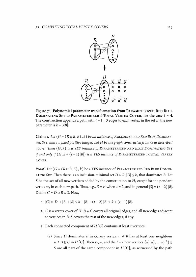
7.1. COMPUTING TOTAL VERTEX COVERS 129
Figure 7.1: Polynomial parameter transformation from Parameterized Red BlueDominating Set to Parameterized t-Total Vertex Cover, for the case t = 4.e construction appends a path with t − 1 = 3 edges to each vertex in the set B; the new
parameter is k + 3∣B∣.
Claim 1. Let (G = (R ⊎ B, E) , k) be an instance of Parameterized Red BlueDominat-
ing Set, and t a xed positive integer. Let H be the graph constructed from G as described
above. en (G , k) is a YES instance of Parameterized Red Blue Dominating Set
if and only if (H, k + (t − 1) ∣B∣) is a YES instance of Parameterized t-Total Vertex
Cover.
Proof. Let (G = (R ⊎ B, E) , k) be a YES instance of Parameterized Red Blue Domin-
ating Set.en there is an inclusion-minimal set D ⊆ R, ∣D∣ ≤ k, that dominates B. Let
S be the set of all new vertices added by the construction to H, except for the pendant
vertex wi in each new path.us, e.g., S = ∅ when t = 2, and in general ∣S∣ = (t − 2) ∣B∣.
Dene C = D ∪ B ∪ S. Now,
1. ∣C∣ = ∣D∣ + ∣B∣ + ∣S∣ ≤ k + ∣B∣ + (t − 2) ∣B∣ ≤ k + (t − 1) ∣B∣.
2. C is a vertex cover of H: B ⊆ C covers all original edges, and all new edges adjacent
to vertices in B; S covers the rest of the new edges, if any.
3. Each connected component of H [C] contains at least t vertices:
(a) Since D dominates B in G, any vertex vi ∈ B has at least one neighbour
w ∈ D ⊆ C in H [C].en vi ,w, and the t − 2 new vertices u1i , u
2i , . . . u
t−2i ⊆
S are all part of the same component in H [C], as witnessed by the path

130 CHAPTER 7. TOTAL VERTEX COVER AND TOTAL EDGE COVER
w , vi , u1i , u
2i , . . . u
t−2i .us each vertex vi ∈ B is part of a connected component
of size at least t in H [C].
(b) D is an inclusion-minimal dominating set of B and D ∪ B ⊆ C, and so each
w ∈ D has at least one neighbour vi ∈ B in the graph H [C]. It follows that
each vertex w ∈ D is part of a connected component of size at least t in H [C],
namely the component to which vi belongs.
(c) Each vertex uj
i ∈ S is in the same component in H [C] as the vertex vi ∈ B,
and so uj
i is part of a connected component of size at least t in H [C], namely
the component to which vi belongs.
us C is a t-total vertex cover ofH, of size at most k+(t − 1) ∣B∣.is proves the forward
direction.
To prove the reverse direction, suppose (H, k + (t − 1) ∣B∣) is a YES instance of t-
TotalVertexCover, and let C be a t-total vertex cover ofH of size at most k+(t − 1) ∣B∣.
Consider any path P = (u0i = vi , u1i , u
2i , . . . u
t−2i ,wi) in H consisting of a vertex vi ∈ B
and new vertices added by the construction. Since C is a vertex cover such that each
connected component of G[C] has at least t vertices, we have that ∣P ∩ C∣ ≥ t − 1. Now
suppose there exists a vertex x ∈ P ∖ C. If x = uj
i for some 0 ≤ j ≤ t − 2, then the vertices
uj+1
i , uj+2
i , . . . , ut−2i ,wi form a connected component of H [C] of size strictly less than t, a
contradiction. So one of the following holds:
1. All the t vertices of P are in C, or,
2. vi , u1i , u
2i , . . . , u
t−2i ∈ C, and wi ∉ C.
Let pt be the number of paths of the rst kind in H, and let pt−1 be the number of such
paths of the second kind.ere is exactly one such path corresponding to each vertex
of B, and so pt + pt−1 = ∣B∣.e total number of vertices contributed to C by these paths
is tpt + (t − 1) pt−1, and so the number of vertices in C ∩ R is at most k + (t − 1) ∣B∣ −
(tpt + (t − 1) pt−1) = k − pt. Now let P be a path of the second kind. By denition,
∣P ∩ C∣ = (t − 1), and since each connected component of G [C] has at least t vertices,
there is at least one more vertex x in C that is adjacent in H to one of the vertices, say y,
of P ∩ C.e only possibility is that x ∈ R and y ∈ B, and so at most k − pt vertices in
C ∩ R dominate pt−1 = ∣B∣ − pt vertices in B. Since each vertex of B has a neighbour in R,
at most k vertices in R dominate all of B.
is completes the proof of the theorem.
e reduction employed in the above argument also implies:
7.1. COMPUTING TOTAL VERTEX COVERS 131
Corollary 7.1. For each xed t ≥ 2 the t-Total Vertex Cover problem is NP-hard on
bipartite graphs, and the Parameterized t-TotalVertex Cover problem does not admit
a polynomial kernel on bipartite graphs unless the Polynomial Hierarchy collapses to the
third level.
7.1.2 Fixed Parameter Tractability
We now turn to the xed-parameter tractability of Parameterized t-Total Vertex
Cover. Two special cases of the problem, for the two extreme values namely t = 1
(Parameterized Vertex Cover) and t = k (Parameterized Connected Vertex
Cover), have been studied extensively from the perspective of parameterized algorithms.
e Parameterized Vertex Cover problem is perhaps the most well-studied problem
in parameterized algorithmics. Aer a long series of improvements, the current fastest
FPT algorithm for this problem runs in timeO∗ (1.2738k) [25]. Similarly Parameterized
Connected Vertex Cover also has a history of improvements, and the current fastest
FPT algorithm for this problem runs in time O∗ (2.7606k) [91]. We show in this section
that Parameterized t-Total Vertex Cover is FPT parameterized by the solution size
k for 2 ≤ t ≤ k, by deriving an O∗(16.1k+O(log2 k)) time algorithm for these problems.
Let G = (V , E) be the input graph, and let ∣V ∣ = n. Observe that the set V is a vertex
cover of G.erefore, if ∣V ∣ ≤ k, then we can solve the problem in polynomial time by
checking whether each component of G has at least t vertices. Also, deleting isolated
vertices does not aect the solution. Hence we assume without loss of generality that
∣V ∣ > k, and that G has no isolated vertices. We start with a structural claim which is
useful later.
Claim2. Let G = (V , E) , ∣V ∣ > k be a graphwithout isolated vertices.enG has a t-total
vertex cover of size at most k if and only if G has a t-total vertex cover of size exactly k.
Proof. IfG has a t-total vertex cover, say S, of size exactly k, then S itself is a t-total vertex
cover of G of size at most k. For the other direction, let S be a t-total vertex cover of G
size l < k. Consider any set of k − l vertices T ⊆ (V ∖ S). Since G has no isolated vertex,
each v ∈ T has at least one edge incident on it; since S is a vertex cover of G, the other
end of this edge, say w, is in S. Now notice that every connected component of G[S ∪ T]
has at least t vertices as each connected component of G [S] has at least t vertices and
every vertex of T gets attached to one of the components of G [S].
e number of unlabelled trees on k vertices is known to be singly exponential in k,
and all these trees can be enumerated with polynomial delay:

132 CHAPTER 7. TOTAL VERTEX COVER AND TOTAL EDGE COVER
Fact 3. [12, 97]e number of unlabelled trees on k vertices is at most 2.96k. Moreover, all
non-isomorphic unlabelled trees on k vertices can be enumerated in time O(2.96kkc) for
some constant c independent of k.
From this we get:
Lemma 7.1. All unlabelled forests on k vertices can be enumerated in O∗ (2.96k) time.
Proof. Let F be a forest on k vertices. Add a new vertex v and one edge from v to an
arbitrary vertex of each tree in F, to obtain a tree T on k + 1 vertices. Clearly, the forest
F can be obtained by deleting one vertex (namely v) from T . It follows that a graph is a
forest on k vertices if and only if it can be obtained by deleting a vertex from some tree
on k + 1 vertices.
To enumerate all forests on k vertices, we rst enumerate all trees on k+1 vertices. From
Fact 3, this can be done in O (2.96k+1 (k + 1)c) time where c is a constant independent of
k. For each tree T on k + 1 vertices obtained in this manner, we delete each of its k + 1
vertices, one at a time, to obtain a set of forests. By the above observation, this procedure
yields every forest on k vertices (some of them perhaps many times).e procedure takes
O ((k + 1) 2.96k+1 (k + 1)c) = O∗ (2.96k) time.
We are now ready to prove the main result of this section.
eorem 7.3. For every t ≥ 1 the Parameterized t-Total Vertex Cover problem is
xed-parameter tractable, and can be solved in time O∗ (16.1k+O(log2 k)).
Proof. Observe that any t-total vertex cover, say S, of G is also a vertex cover of G and
hence contains a minimal vertex cover S′ ⊆ S of G.e idea of our proof is to enumerate
all the minimal vertex covers of G of size at most k and then try to expand each one to
a t-total vertex cover of G. We will use Fact 3 and the colour-coding technique of Alon
et al. [4] to do the expansion phase of our algorithm. Our algorithm is based on the
following claim.
Claim 3. A graph G = (V , E) has a t-total vertex cover of size k if and only if there exists
a minimal vertex cover C of G of size at most k, and a subset T ⊆ V ∖ C of size k − ∣C∣,
such that there exists a forest F on k vertices which is isomorphic to a spanning subgraph
of G[C ∪ T], and in which each connected component has at least t vertices.
Proof. IfG has a t-total vertex cover S of size k, then by denition S is a vertex cover ofG.
Let C be any minimal vertex cover contained in S, and let T = S ∖ C.en ∣T ∣ = k − ∣C∣,
and each connected component of G [C ∪ T] = G [S] has, from the denition of a t-total
7.1. COMPUTING TOTAL VERTEX COVERS 133
vertex cover, at least t vertices. Let F be a forest formed by picking one spanning tree
from each connected component of G [S].en F satises the conditions of the claim.
Conversely, let there exist a minimal vertex cover C ofG, a set T ⊆ V ∖C of size k− ∣C∣,
and a forest F on k vertices that is isomorphic to a spanning subgraphG′ = (S = C ∪ T , E′)
of G[C ∪ T], and in which each connected component has at least t vertices. Since C ⊆ S,
S is a vertex cover of G. Also ∣S∣ = ∣C ∪ T ∣ = k. Now since G′ is a subgraph of G [S], and
each connected component of G′ contains at least t vertices, each connected component
of G [S] has at least t vertices. It follows that S is a t-total vertex cover of G of size k.
If G has a t-total vertex cover of size at most k, then from Claim 2 we know that G
has a t-total vertex cover of size exactly k. Let S be a xed t-total vertex cover of G of size
exactly k, if there exists one. From Claim 3 we get that S contains an inclusion-minimal
vertex cover C of G, of size at most k. A “colouring” of the vertex set V of G is a function
from V to some specied set of “colours”. A “good” colouring of V is a colouring in which
the vertices in S are all distinctly coloured.
Our algorithm tries to nd S by mimicking Claim 3. First we enumerate all inclusion-
minimal vertex covers ofG of size at most k.is can be done in timeO∗ (2k) by a simple
2-way branching on edges — for every edge at least one of its endpoints should be in any
vertex cover. For each such vertex cover C, we do the following:
1. Colour each v ∈ C with a distinct colour from 1, 2, . . . , ∣C∣.
2. Let ℓ = k − ∣C∣. Colour the vertices of the independent set V ∖ C uniformly at
random with ℓ new colours 1, 2, . . . , ℓ.
Observe that ∣S ∖ C∣ = ℓ.e number of ways of colouring the vertices in S ∖ C with ℓ
distinct colours is ℓ!, and the total number of ways of colouring these vertices with these ℓ
colours is ℓℓ.e random colouring described above will therefore yield a good colouring
of V with probability ℓ!/ℓℓ ≥ e−ℓ.
We now check if the random colouring is a good colouring. For this, we iterate
through all unlabelled forests on k vertices, and check if at least one of these forests is
isomorphic to a spanning forest F of G [S], where each connected component of F has at
least t vertices. By Lemma 7.1, we can iterate through all such forests in O∗ (2.96k) time.
To check if a given forest F on k vertices is isomorphic with such a spanning forest F of
G [S], we do the following:
1. We check if there is at least one tree in F that has less than t vertices. If yes, then
we reject F.
134 CHAPTER 7. TOTAL VERTEX COVER AND TOTAL EDGE COVER
2. Next we check if there is a colourful subgraph (one in which each vertex has a
distinct colour) isomorphic to F in the coloured graph obtained above. Since F is
of treewidth at most 1, this can be done in O (2k ⋅ k ⋅ n2) time [8, Corollary 6]. If
such a subgraph is present, then F satises the requirements of Claim 3, and so we
return Yes; the underlying uncoloured graph of this colourful subgraph is a t-total
vertex cover of G of size at most k. Otherwise we reject the forest F.
If the above check rejects all unlabelled forests on k vertices, then we return No: this
colouring is not a good colouring.
Observe that if the input graph G has a t-total vertex cover of size k, then the above
algorithm will discover this t-total vertex cover with probability at least e−ℓ, and so will
return Yes with probability at least e−ℓ. If the input graph G is a No instance, then the
algorithm will always return No. e expected number of times the algorithm has to
be repeated before it nds a t-total vertex cover of size k of G, if it exists, is thus eℓ.e
expected running time of this procedure is thus
O⋆ (k
∑ℓ=0
2k−ℓ × eℓ × 2.96k × 2k) = O⋆ ((2 × 2.96 × 2)k×
k
∑ℓ=0
((e
2)ℓ
))
= O⋆ ((5.92e)k) = O⋆ (16.1k) .
To obtain a deterministic algorithm we have to replace the randomized step of the
algorithm— where we colour the vertices of G[V ∖C] uniformly at random by ℓ colours
— with a deterministic procedure. We do this using the so-called (n, ℓ, ℓ)-perfect hash
families.
An (n, ℓ, ℓ)-perfect hash familyH is a set of functions from 1, . . . , n to 1, . . . , ℓ
such that for every subset S ⊆ 1, . . . , n of size ℓ there exists a function f ∈H such that f
is injective on S.at is, such that for all i , j ∈ S, f (i) ≠ f ( j).ere exists a construction
of an (n, ℓ, ℓ)-perfect hash family of size O(eℓ ⋅ ℓO(log ℓ) ⋅ log n) and one can produce this
family in time linear in the output size [93].
Let n = ∣V ∖ C∣. To derandomize our algorithm, we construct an (n, ℓ, ℓ)-perfect
hash familyH from 1, . . . , n to 1, . . . , ℓ. is has to be done only once during the
algorithm. Now we replace the second step in the colouring process with the following:
2’. Instead of colouring the vertices of V ∖ C uniformly at random with ℓ colours and
checking if this yields a good colouring, we “colour” the vertices of V ∖C with each
function inH, in turn. For each such colouring, we check if it is a good colouring
as before.
7.2. COMPUTING TOTAL EDGE COVERS 135
IfG has a t-total vertex cover S of size k, then from the denition of an (n, ℓ, ℓ)-perfect
hash family, it follows that at least one of the functions inH will result in a good colouring
of V . us, if G has a t-total vertex cover S of size k, then this algorithm will always
discover S and return Yes. If the input graph G is a No instance, then the algorithm will
always return No. Instead of the multiplicative factor of eℓ —which came from repeating
the randomized algorithm these many times — in the running time of the randomized
procedure, the derandomized version incurs the following costs:
1. An additive cost of O(eℓ ⋅ ℓO(log ℓ) ⋅ log n) to compute the hash family, and
2. A multiplicative factor of O(eℓ ⋅ ℓO(log ℓ) ⋅ log n) which arises from repeating the
check for a good colouring once for each function in the hash family.
e running time of the derandomized algorithm is thus
O∗ (k
∑ℓ=0
2k−ℓ × eℓ × ℓO(log ℓ) × 2.96k × 2k) =
O∗ ((2 × 2.96 × 2)k×
k
∑ℓ=0
((e
2)ℓ
× ℓO(log ℓ))) =
O∗ ((11.84)k× kO(log k) × (
e
2)k
) =
O∗ (16.1k+O(log2 k)) .
is concludes the proof of the theorem.
7.2 Computing Total Edge Covers
We now consider the t-Total Edge Cover problem. For t = 1 this problem becomes the
EdgeCover problem, which has long been known to be solvable in polynomial time [96].
e problem is NP-complete for all t ≥ 2 [50,eorem 3]. In this section we investigate
the parameterized complexity of the Parameterized t-Total Edge Cover problem for
t ≥ 2. We rst study the kernelization complexity of the problem, and improve the size of
the kernels for all t ≥ 2.en we take up the xed parameter tractability of this problem,
and obtain an FPT algorithm with a signicantly improved running time.
In our analysis we make use of a dierent formulation of the problem, other than the
one presented at the beginning of this chapter.e following fact, culled from the proof
of a theorem in the previous work due to Fernau and Manlove [50,eorem 16], helps us
show that the two formulations are equivalent.
136 CHAPTER 7. TOTAL VERTEX COVER AND TOTAL EDGE COVER
Fact 4. [50] In any connected graph G with n vertices, and for any t < n, there exists a
minimal t-total edge cover, say S, of G such that the graph G(S) induced by the edge set S
is acyclic.
7.2.1 Kernelization Complexity
Fernau and Manlove [50] observed the following simple vertex kernel of size at most 2k
for t-Total Edge Cover [50] : any edge in a graph covers exactly 2 vertices, and a YES
instance of the problem has an edge cover of size (number of edges) at most k, and so
such an instance cannot have more than 2k vertices. In other words, if the input instance
has more than 2k vertices, then the answer is NO. Otherwise, the input instance itself
forms a kernel on at most 2k vertices. We can improve this bound on the kernel size for
larger values of t by observing the following:
Lemma 7.2. Given a graph G = (V , E) and a non-negative integer k, solving the t-Total
Edge Cover instance (G , k) is equivalent to solving the following problem: does there
exist a partition of the vertex set V into q parts V1, . . . ,Vq, for some q, such that (i) G[Vi]
is connected, (ii) ∣Vi ∣ ≥ t + 1 for each 1 ≤ i ≤ q, and (iii)∑q
i=1(∣Vi ∣ − 1) ≤ k?
Proof. Let (G = (V , E) , k) be an instance of Parameterized t-Total Edge Cover and
let S be an edge-minimal t-total edge cover of G. Let V1, . . . ,Vq be the vertex sets of the
connected components ofG(S) = (V , S). It directly follows fromFact 4 and the properties
of S given in the denition of Parameterized t-Total Edge Cover that V1, . . . ,Vq
satisfy all the conditions in the statement of the lemma. For the reverse direction, observe
rst that the edges of a spanning tree of any connected graph form an edge cover of the
graph. Now, if V1, . . . ,Vq satisfy all the conditions in the statement of the lemma, then
let Si be the edges of a spanning tree of G [Vi], for 1 ≤ i ≤ q, and let S = ⋃q
i=1 Si . Observe
now that S has the properties stated in the denition of Parameterized t-Total Edge
Cover.
We use this reformulation to get smaller bounds on the kernel size for Parameterized
t-Total Edge Cover.
eorem 7.4. Parameterized t-Total Edge Cover admits a vertex kernel of size t+1tk.
Proof. Let (G = (V , E) , k) be a Yes instance of Parameterized t-Total Edge Cover.
By Lemma 7.2, there exists a partition of V into q parts of the kind stated in Lemma 7.2.
Now ∣Vi ∣ ≥ t+1 Ô⇒ ∣Vi ∣−1 ≥ t Ô⇒ ∑q
i=1 (∣Vi ∣ − 1) ≥ qt. By Lemma 7.2,∑q
i=1 (∣Vi ∣ − 1) ≤
k, and so qt ≤ k, and q ≤ kt. Also,∑
q
i=1 (∣Vi ∣ − 1) ≤ k Ô⇒ ∑q
i=1 ∣Vi ∣ ≤ k + q ≤ k + kt= t+1
tk,
and so G has at most t+1tk vertices.
7.2. COMPUTING TOTAL EDGE COVERS 137
us, if the input graphG hasmore than t+1tk vertices, then the answer isNo.erefore
we can assume without loss of generality that the input graph has at most t+1tk vertices,
and so any exact algorithm for the problem is in fact an FPT algorithm. In particular we
have:
Corollary 7.2. If Parameterized t-Total Edge Cover has an exact exponential time
algorithm that runs inO∗ (c f (∣V ∣)) time on an input instance (G = (V , E) , k) for some con-
stant c and function f (), then the problem has an FPT algorithm that runs inO∗ (c f (t+1tk))
time.
7.2.2 Fixed Parameter Tractability
We now present an exact exponential-time algorithm for Parameterized t-Total Edge
Cover which runs in O∗ (2n+O(
√
n)) time where n is the number of vertices in the input
graph. By Corollary 7.2 this yields an FPT algorithm for the problemwhich runs inO∗ (ck)
time for some xed constant c.is is a signicant improvement over the previous best
upper bound of O∗ ((2k)2k) [50].
Let (G = (V , E), k) be an input instance of Parameterized t-Total Edge Cover,
and let ∣V ∣ = n. We start by enumerating all unordered partitions of n. An unordered
partition of a positive integer n is a way of writing n as a sum of positive integers, where
the order of the summands is ignored. By the Hardy-Ramanujan asymptotic formula, n
has at most 2O(
√
n) unordered partitions [67].e partitions of n can be generated with
constant average delay [112], and so we can enumerate all unordered partitions of n in
2O(
√
n) time.
We consider those partitions of n of the form n = n1 + n2 +⋯ + nq which satisfy the
following conditions of Lemma 7.2:
1. ∑q
i=1(∣ni ∣ − 1) ≤ k
2. ∣ni ∣ ≥ t + 1
For each such partition of n, we check if there exists a partition of the vertex set V into q
parts V1, . . . ,Vq such that
1. ∣Vi ∣ = ni for 1 ≤ i ≤ q, and
2. each induced subgraph G[Vi] is connected.
To do these latter checks, we construct the q lists
Li = V ′ ⊆ V ∣ ∣V ′∣ = ni and G [V ′] is connected
138 CHAPTER 7. TOTAL VERTEX COVER AND TOTAL EDGE COVER
for 1 ≤ i ≤ q. For 1 ≤ i ≤ q we compute the polynomials
Pi = ∑V ′∈L i
zχ(V′)
where z is a formal variable and χ (V ′) is the (binary number represented by the) char-
acteristic vector of V ′ ⊆ V . at is, let V = v1, v2, . . . , vn. en χ (V ′) is a bit vector
with ∣V ∣ bits where, for 1 ≤ j ≤ ∣V ∣, the jth bit of χ (V ′) is 1 if and only if v j ∈ V ′. We
treat χ (V ′) as a binary number in all computations.e lists Li and the polynomials Pi
can be computed in O∗ (2n) time, by enumerating all subsets of V . We now compute the
product
Q = P1 × P2 ×⋯ × Pq
in the given order, with a small modication: at each step, given the partial product Qi of
the rst i terms, we rst compute Qi ×Pi+1.en we delete all those terms αzβ in Qi ×Pi+1
where (the binary representation of) β does not contain exactly∑i+1j=1 n j 1s, and set Qi+1 to
be the resulting polynomial.is pruning operation ensures that the partial product Qi ,
for 1 ≤ i ≤ q, represents exactly those sets of size∑ij=1 n j that can be obtained by taking the
union of one set each from L1, L2, . . . , Li . Observe that the product Qq = Q is non-zero if
and only if there exists a partition of V into q parts satisfying the conditions stated above.
e degree of each polynomial involved in themultiplications is at most 2∣V ∣−1 = 2n−1,
and so, using the Fast Fourier Transform, we can multiply two of these polynomials in
O (2n log 2n) = O (n2n) time [26, Chapter 30]. We have to perform at most q ≤ n such
multiplications to compute Q, and so given the Pis we can compute Q in O (n22n) =
O∗ (2n) time.e running time of this algorithm is thus 2O(
√
n) × (O∗ (2n) +O∗ (2n)) =
O∗ (2n+O(
√
n)), and so we have:
eorem 7.5. t-Total Edge Cover can be solved in O∗ (2n+O(
√
n)) time, where n is the
number of vertices in the input graph.
From this theorem and Corollary 7.2 we get:
eorem 7.6. Parameterized t-Total Edge Cover can be solved in O∗ (2t+1tk+O(
√
k))
time.
e above algorithm uses exponential space, for constructing the lists Li . We can use
an approach similar to the one used in Section 7.1.2 to get an FPT algorithm which runs
in polynomial space. Specically, we enumerate all unordered partitions (n1, . . . nq) of
n where n − k ≤ q ≤ nt+1, such that ni ≥ t + 1 and ∑
q
i=1(ni − 1) ≤ k. As mentioned above,
7.3. CONCLUSION 139
this can be done in O⋆(2√
n) time. For each such partition, we enumerate all trees with
number of vertices ni ; 1 ≤ i ≤ q. As mentioned above, this can be done in O⋆(2.96n)
time.en, for each enumerated q-tuple of trees (T1, . . . , Tq), we test whether the forest
T1 ⊎ T2 ⊎⋯ ⊎ Tq is a subgraph of G. Since the forest has treewidth one and has the same
number of vertices as G, this test for subgraph isomorphism can be done in O∗(2n) time
and polynomial space [7,eorem 5]. Combining this with Corollary 7.2 we get:
eorem 7.7. Parameterized t-Total Edge Cover can be solved in O∗ (2t+1tk+O(
√
k))
time and using polynomial space.
7.3 Conclusion
We study the eect of imposing some natural connectivity constraints on the subgraph
induced by the solution set for two classical problems, namely Vertex Cover and Edge
Cover.ese problems exhibit contrasting behaviour with respect to classical complexity:
Vertex Cover is NP-hard while Edge Cover is solvable in polynomial time. For both
these problems, the additional constraint imposed is that each connected component of
the subgraph induced by the solution set be at least as large as some specied number t;
these problems were introduced by Fernau and Manlove [50], who named the problems
t-Total Vertex Cover and t-Total Edge Cover, respectively.ey showed that these
problems are NP-hard for t ≥ 2, and initiated the study of the parameterized complexity
of these problems when the parameter is the solution size k. We take this study further,
and improve on their results.
In both cases we see that adding a connectivity constraint (each component of the
solution must have at least a certain number of vertices/edges from the solution) causes
a drastic change in the computational complexity of the problem. In the case of t-
Total Edge Cover, the shi is from polynomial-time computability to NP-hardness,
as had been observed earlier [50]. We show that a similar shi occurs in the case of
the parameterized version Parameterized t-Total Vertex Cover of the NP-hard
problem t-Total Vertex Cover. As is well known, for t = 1 the problem has a linear
vertex kernel [23]. In contrast, we showed that for any t ≥ 2 the Parameterized t-Total
Vertex Cover problem has no polynomial-size kernel unless the Polynomial Hierarchy
collapses, which is considered unlikely. We also show that both these problems have
FPT algorithms that run in time O∗ (ck) for dierent constants c.ese results improve
known bounds for these problems [50].
One interesting direction of future research would be to examine the eect of such
connectivity constraints on other parameterized graph problems. Another would be

140 CHAPTER 7. TOTAL VERTEX COVER AND TOTAL EDGE COVER
to try to improve the base c of the exponent of the running times that we obtained for
Parameterized t-Total Vertex Cover and Parameterized t-Total Edge Cover.
Recall —eorem 7.3 — that our algorithm for the Parameterized t-Total Vertex
Cover problem runs in O⋆(16.1k) time. For the three special values t = 1, t = 2 and t = k,
the Parameterized t-Total Vertex Cover problem is known to be solvable in O⋆(ck)
time for have much smaller values of c, namely c = 1.2738, c = 2.3655 and c = 2.7606,
respectively [25, 50, 91]. It will be interesting to see if the value of c for the general case
can be brought closer to these smaller values.

Part IV
Conclusion
141

CHAPTER 8
Conclusion
Polynomial-time preprocessing is a time-tested way of dealing with instances of
hard problems. It has oen been known to result in surprising gains in the speed
with which the problem can be solved. e following quote from Alber et al.’s
early work [1] on polynomial-time data reduction for Dominating Set portrays a notable
example of such an occurrence, from Weihe’s practical work [108, 109] on Red Blue
Dominating Set:
Weihe . . . gave a striking example when dealing with the NP-complete
RedBlueDominating Setproblemappearing in the context of the European
railroad network. In a preprocessing phase, he applied two simple data re-
duction rules again and again until no further application was possible.e
impressive result of his empirical study was that each of his real-world in-
stances was broken into very small pieces such that for each of these a simple
brute-force approach was sucient to solve the computationally hard prob-
lems eciently and optimally.
In this thesis we saw some examples of polynomial-time preprocessing applied to
dierent hard graph problems. In each case the eciency of the method was analysed
using the mathematical framework provided by the notion of kernelization from Para-
meterized Complexityeory. We also proved some lower bounds on kernel size. In
this concluding chapter we look back on the results obtained, and ponder on possible
directions of future work.
143
144 CHAPTER 8. CONCLUSION
We rst focused our attention on the Parameterized Dominating Set problem.
While this problem is known to be W[2]-complete and thus unlikely to have kernels
of any size on general graphs, we showed that the problem has polynomial kernels on
larger classes of graphs than was known before our work. Specically, we showed that for
every xed j ≥ i ≥ 1, the Parameterized Dominating Set problem restricted to graphs
that do not have Ki , j as a subgraph is FPT and has a polynomial kernel. We described a
polynomial-time algorithm that, given a Ki , j-free graph G and a non-negative integer k,
constructs a graph H (the “kernel”) and an integer k′ such that (1) G has a dominating
set of size at most k if and only if H has a dominating set of size at most k′, (2) H has
O(( j + 1)i+1k i2
) vertices, and (3) k′ = O(( j + 1)i+1k i2
).
Since d-degenerate graphs do not have Kd+1,d+1 as a subgraph, this result directly
implies a polynomial kernel on O((d + 2)d+2k(d+1)2) vertices for the Parameterized
Dominating Set problem on d-degenerate graphs, solving an open problem posed by
Alon and Gutner [2, 65].
Dom et al. [39] have shown that Parameterized Dominating Set restricted to d-
degenerate graphs has no kernel of size polynomial in both k and d unless the Polynomial
Hierarchy collapses to the third level.is implies that our kernel size is nearly the best
possible for the problem on this class of graphs.
e most general class of graphs for which a polynomial kernel was previously
known for Parameterized Dominating Set is the class of Kh-topological-minor-free
graphs [65]. Graphs of bounded degeneracy are the most general class of graphs for which
an FPT algorithm was previously known for this problem [3]. Kh-topological-minor-free
graphs are Ki , j-free for suitable values of i , j (but not vice versa), and so our results show
that Parameterized Dominating Set has both FPT algorithms and polynomial kernels
on strictly more general classes of graphs.
Using the same techniques, we also obtained an O ( jk i) vertex-kernel for the Para-
meterized Independent Dominating Set problem on Ki , j-free graphs.
One interesting direction of future work is to try to demonstrate (no) kernels of size
f (d) ⋅ kc for the Parameterized Dominating Set problem on d-degenerate graphs,
where c is independent of d. Note that the result of Dom et al. mentioned above does
not suggest that such kernels are unlikely. Dell and van Melkebeek [34] have recently
developed a lower-bound technique which allows them to show, inter alia, that the vertex
deletion problem for any nontrivial hereditary graph class has no kernel of size O(k2−є)
for any є > 0. A second interesting open problem is whether this new machinery can be
extended to show that the Parameterized Dominating Set problem does not have
kernels of size f (d) ⋅kc on d-degenerate graphs. Cygan et al. [28] have recently shown that
Parameterized Connected Dominating Set has no polynomial kernels on graphs of
145
degeneracy d ≥ 2 unless the Polynomial Hierarchy collapses to the third level. A third
set of interesting open problems consists of nding if the natural parameterized versions
of other NP-hard variants of Dominating Set such as Efficient Dominating Set,
AnnotatedDominating Set, RomanDomination, MaximumMinimalDominating
Set, and many others∗ have polynomial kernels and/or FPT algorithms on d-degenerate
graphs and beyond.
e second graph domination problem which we took up for study was the Para-
meterized Connected Dominating Set problem.is problem is also known to be
W[2]-complete on general graphs. We investigated the eect of excluding short cycles, as
subgraphs, on the kernelization complexity of Parameterized Connected Dominat-
ing Set. It turned out that the ParameterizedConnectedDominating Set problem is
hard on graphs with small cycles, and becomes progressively easier as the girth increases.
More precisely, we obtained the following kernelization landscape: Parameterized
Connected Dominating Set
• does not have a kernel of any size on graphs of girth 3 or 4 (since the problem is
W[2]-hard);
• admits a kernel of size 2kk3k on graphs of girth at least 5;
• has no polynomial kernel (unless the Polynomial Hierarchy collapses to the third
level) on graphs of girth at most 6, and,
• has a cubic (O(k3)) vertex kernel on graphs of girth at least 7.
e most important technical contribution in this work is the third result, which says
that the Parameterized Connected Dominating Set problem has no polynomial
kernels on graphs with girth at most 6. On the way to proving this result we introduced
a new problem, namely Parameterized Fair Connected Colours, and showed that
this problem has no polynomial kernels. is intermediate result is interesting in its
own right; we feel that it could be used to show kernelization lower bounds for other
connectivity problems on graphs that exclude small cycles. Most known kernelization
and FPT results for W-hard problems are for graph classes characterized by excluded
minors. Our results add to the small but growing collection of such results for graph
classes characterized by excluded subgraphs. One interesting direction of future work is
to study how the exclusion of small cycles — or other small graphs — as subgraphs aects
the kernelization complexity of other W-hard parameterized graph problems.
∗ Please see the Compendium [27] for the denitions of these and other related problems.
146 CHAPTER 8. CONCLUSION
We now turned our attention to graph covering problems. In these the objective is to
nd a small set of vertices or edges of a graph whose removal deletes some structure from
the graph. We rst looked at the Parameterized Pathwidth-One Vertex Deletion
problem, in which the objective is to obtain a graph of pathwidth at most one by vertex
deletion. We initiated the study of the parameterized complexity of this problem, para-
meterized by the solution size k. We showed that the problem has a quartic vertex-kernel:
We showed that, given an input instance (G = (V , E), k) where ∣V ∣ = n, we can construct,
in polynomial time, an instance (G′, k′) such that (i) (G , k) is a Yes instance if and only
if (G′, k′) is a Yes instance, (ii) G′ has O(k4) vertices, and (iii) k′ ≤ k. We also derived an
FPT algorithm for the problem that runs in O(7kk ⋅ n2) time.ese results are based on
two dierent characterizations of graphs of pathwidth at most one: the rst, as a collection
of caterpillars, and the second, as the set of graphs which exclude the graphs K3 and T2 as
minors.
Cygan et al. recently improved these bounds: they found an FPT algorithm which
runs in O⋆(4.65k) time, and a kernel of size O(k2) [29].
A challenging open problem is to try to solve the analogous problem for larger values
of pathwidth. We know by results from graph minor theory that for any positive integer
c, the Pathwidth c Vertex Deletion problem, dened analogously to Parameterized
Pathwidth-One Vertex Deletion, is FPT parameterized by the solution size.is is
so because for each xed c, the set of Yes instances for this problem form a minor-closed
class. However, for c = 2, the number of graphs in the obstruction set is already a hundred
and ten [76], and so our approach would probably be of limited use for c ≥ 2.us the
interesting open problems for c ≥ 2 are: (i) Can we get an O∗(dk) FPT algorithm for the
problem for some constant d, and (ii) Does the problem have a polynomial kernel?
e second graph covering problem which we looked at was the Connected Feed-
back Vertex Set problem, where the question is whether the input graph has a small
feedback vertex set which induces a connected subgraph.e related Parameterized
Feedback Vertex Set problem is one of the best studied problems in parameterized
complexity. In contrast, the ParameterizedConnected FeedbackVertex Set had not
been investigated prior to our work, in which we derived the rst FPT algorithms for the
problem. We showed that the problem can be solved inO⋆(46.2k) time on general graphs,
and inO⋆(2O(
√
k log k)) time on graphs excluding a xed graph H as a minor.ese results
imply that the problem has kernels of size 46.2k on general graphs and 2O(
√
k log k) on
H-minor free graphs. We further showed that the problem is unlikely to have polynomial
kernels on general graphs.
On the way to proving the FPT results for Parameterized Connected Feedback
Vertex Set, we establish that two variants of the well-studied Parameterized Steiner

147
Tree problem, namely Parameterized Directed Steiner Out-Tree and Parameter-
ized Group Steiner Tree, are FPT when parameterized by the number t of terminals.
We show that both these problems can be solved in O⋆(2t) time and polynomial space.
We nd these FPT algorithms to be of independent interest, and believe that it could be
useful for obtaining parameterized algorithms for other connectivity problems.
When H is an apex graph, recent meta-results due to Fomin et al. [56] imply that the
problem has a polynomial kernel on H-minor free graphs. Very recently, Cygan et al. [30]
achieved a signicant breakthrough in solving connectivity problems using which they
show, inter alia, that both Parameterized Feedback Vertex Set and Parameterized
Connected Feedback Vertex Set can be solved in randomized 3knO(1) time.
Note that our FPT algorithm for the problem directly implies a polynomial-time
approximation algorithm with approximation factor n/c log n for any constant c, where
n is the number of vertices in the input graph. Somewhat surprisingly, this is the best
polynomial-time approximation algorithm known for this problem. A very interesting
open problem is thus to nd a polynomial-time approximation algorithm for the Connec-
ted Feedback Vertex Set problem with an approximation ratio asymptotically better
than n/ log n, or to show that no such algorithm exists. It would also be interesting to
nd whether Parameterized Connected Feedback Vertex Set admits a polynomial
kernel on graphs excluding an arbitrary xed graph H as a minor.
Finally, we looked at variants of two well-studied graph covering problems — Vertex
Cover and EdgeCover—with additional “partial” connectivity constraints. Specically,
for each xed 2 ≤ t ≤ k we imposed the additional requirement that each connected
component of the graph induced by the solution have
• at least t vertices for Vertex Cover, and called the problem t-Total Vertex
Cover;
• at least t edges from the solution for Edge Cover, and called the problem t-Total
Edge Cover.
Both these problems are known to be NP-hard for each 2 ≤ t ≤ k. We studied the
parameterized complexity of these problems when the parameter is the solution size k.
We showed that
• both problems remain xed-parameter tractable with these restrictions, with run-
ning times of the form O∗ (ck) for some constant c > 0 in each case;
• for 2 ≤ t ≤ k, t-Total Vertex Cover has no polynomial kernel unless the Polyno-
mial Hierarchy collapses to the third level, and,

148 CHAPTER 8. CONCLUSION
• for t2 ≤ t ≤ k, t-Total Edge Cover has a linear vertex kernel of size t+1tk.
ese results signicantly improve earlier work on these problems. Our no-poly-kernel
result for t-Total Vertex Cover, and the known NP-hardness result for t-Total Edge
Cover, are in stark contrast to the fact that Vertex Cover has a 2k vertex kernel, and
that Edge Cover is solvable in polynomial time.ese illustrate how even the slightest
connectivity requirement results in a drastic change in the tractability of problems.
Our algorithm for the Parameterized t-Total Vertex Cover problem runs in
O⋆(16.1k) time. For the three special values t = 1, t = 2 and t = k, the Parameterized
t-Total Vertex Cover problem is known to be solvable in O⋆(ck) time for have much
smaller values of c, namely c = 1.2738, c = 2.3655 and c = 2.7606, respectively [25, 50, 91].
One interesting open problem is to nd whether the value of c for the Parameterized
t-Total Vertex Cover problem can be brought closer to these smaller values. An-
other, more general direction of future research would be to examine the eect of partial
connectivity constraints on other parameterized graph covering problems.
•
Bibliography
1. Jochen Alber, Michael R. Fellows, and Rolf Niedermeier. Polynomial-time data
reduction for Dominating Set. Journal of the ACM, 51(3):363–384, 2004.
2. Noga Alon and Shai Gutner. Kernels for the Dominating Set Problem on Graphs
with an Excluded Minor. Technical Report TR08-066,e Electronic Colloquium
on Computational Complexity (ECCC), 2008. URL http://eccc.hpi-web.de/eccc-reports/2008/TR08-066/index.html. A revised version [65] has beenpublished in the proceedings of IWPEC 2009.
3. Noga Alon and Shai Gutner. Linear time algorithms for nding a dominating set of
xed size in degenerated graphs. Algorithmica, 54(4):544–556, 2009.
4. Noga Alon, Raphael Yuster, and Uri Zwick. Color-coding. Journal of the ACM, 42
(4):844–856, 1995.
5. Noga Alon, Lajos Rónyai, and Tibor Szabó. Norm-graphs: Variations and applica-
tions. Journal of Combinatorialeory, Series B, 76(2):280–290, 1999.
6. Carme Álvarez and Maria J. Serna. The Proper Interval Colored Graph problem for
caterpillar trees. Electronic Notes in Discrete Mathematics, 17:23 – 28, 2004.
7. Omed Amini, Fedor V. Fomin, and Saket Saurabh. Counting subgraphs via ho-
momorphisms. In Automata, Languages and Programming, 36th International Col-
loquium, ICALP 2009, Rhodes, Greece, July 5-12, 2009, Proceedings, Part I, volume
5555 of LNCS, pages 71–82. Springer, 2009.
149
150 BIBLIOGRAPHY
8. Omed Amini, Fedor V. Fomin, and Saket Saurabh. Counting subgraphs via homo-
morphisms. Full version manuscript, available online at http://www.ii.uib.no/~fomin/articles1/si.pdf, 2009.
9. Stefan Arnborg, Andrzej Proskurowski, and Detlef Seese. Monadic Second Order
Logic, Tree Automata and ForbiddenMinors. In Computer Science Logic, 4thWork-
shop, CSL ’90, Heidelberg, Germany, October 1-5, 1990, Proceedings, volume 533 of
LNCS, pages 1–16. Springer, 1990.
10. S. F. Assmann, G.W. Peck,MaciejM. Sysło, and J. Zak. The bandwidth of caterpillars
with hairs of length 1 and 2. SIAM Journal on Algebraic and Discrete Methods, 2(4):
387–393, 1981.
11. Giorgio Ausiello, Pierluigi Crescenzi, Giorgio Gambosi, Viggo Kann, Alberto
Marchetti-Spaccamela, and Marco Protasi. Complexity and approximation — Com-
binatorial optimization problems and their approximability properties. Springer-
Verlag, 1999.
12. Terry Beyer and Sandra Mitchell Hedetniemi. Constant time generation of rooted
trees. SIAM Journal on Computing, 9(4):706–712, 1980.
13. Hans L. Bodlaender. On disjoint cycles. International Journal of Foundations of
Computer Science, 5(1):59–68, 1994.
14. Hans L. Bodlaender. A linear-time algorithm for nding tree-decompositions of
small treewidth. SIAM Journal on Computing, 25(6):1305–1317, 1996.
15. Hans L. Bodlaender, Rodney G. Downey, Michael R. Fellows, and Danny Hermelin.
On problems without polynomial kernels. Journal of Computer and System Sciences,
75(8):423–434, 2009.
16. Hans L. Bodlaender, Corinne Feremans, Alexander Grigoriev, Eelko Penninkx, René
Sitters, and Thomas Wolle. On the minimum corridor connection problem and
other generalized geometric problems. Computational Geometry, 42(9):939–951,
2009.
17. Hans L. Bodlaender, Fedor V. Fomin, Daniel Lokshtanov, Eelko Penninkx, Saket
Saurabh, and Dimitrios M. Thilikos. (Meta) Kernelization. In 50th Annual IEEE
Symposium on Foundations of Computer Science, FOCS 2009, October 25-27, 2009,
Atlanta, Georgia, USA, pages 629–638. IEEE, 2009.
151
18. Hans L. Bodlaender, Stéphan Thomassé, and Anders Yeo. Kernel Bounds for
Disjoint Cycles and Disjoint Paths. InAlgorithms - ESA 2009, 17th Annual European
Symposium, Copenhagen, Denmark, September 7-9, 2009. Proceedings, volume 5757
of LNCS, pages 635–646, 2009.
19. Béla Bollobás. Extremal graph theory. Dover Publications, 2004.
20. Béla Bollobás and Andrewomason. Proof of a conjecture of Mader, Erdös and
Hajnal on topological complete subgraphs. European Journal of Combinatorics, 19
(8):883–887, 1998.
21. R. L. Bryant, Nancy G. Kinnersley, Michael R. Fellows, and Michael A. Langston.
On Finding Obstruction Sets and Polynomial-Time Algorithms for Gate Matrix
Layout. In Proceedings of the 25th Allerton Conference on Communication, Control
and Computing, pages 397–398, 1987.
22. Yixin Cao, Jianer Chen, and Yang Liu. On Feedback Vertex Set: New Measure and
New Structures. In HaimKaplan, editor,Algorithmeory - SWAT 2010, 12th Scand-
inavian Symposium and Workshops on Algorithmeory, Bergen, Norway, June 21-
23, 2010, volume 6139 of LNCS, pages 93–104. Springer, 2010.
23. Jianer Chen, Iyad A. Kanj, and Weijia Jia. Vertex Cover: Further observations and
further improvements. Journal of Algorithms, 41(2):280–301, 2001.
24. Jianer Chen, Henning Fernau, Iyad A. Kanj, and Ge Xia. Parametric Duality and
Kernelization: Lower Bounds and Upper Bounds on Kernel Size. SIAM Journal on
Computing, 37(4):1077–1106, 2007.
25. Jianer Chen, Iyad A. Kanj, and Ge Xia. Improved upper bounds for vertex cover.
eoretical Computer Science, 411(40-42):3736–3756, 2010.
26. omas H. Cormen, Charles E. Leiserson, Ronald L. Rivest, and Cliord Stein.
Introduction to Algorithms. e MIT Press, second edition, 2001.
27. Pierluigi Crescenzi, Viggo Kann, Magnús M. Halldórsson, Marek Karpinski, and
Gerhard Woeginger. A compendium of NP optimization problems, 2000. URL
http://www.nada.kth.se/~viggo/wwwcompendium/wwwcompendium.html.
28. Marek Cygan, Marcin Pilipczuk, Michał Pilipczuk, and Jakub Onufry Wojtaszczyk.
Kernelization Hardness of Connectivity Problems in d-Degenerate Graphs. In
Dimitrios M.ilikos, editor, Grapheoretic Concepts in Computer Science - 36th

152 BIBLIOGRAPHY
International Workshop, WG 2010, Zarós, Crete, Greece, June 28-30, 2010. Revised
Papers, volume 6410 of LNCS, pages 147–158, 2010.
29. Marek Cygan, Marcin Pilipczuk, MichałPilipczuk, and Jakub Onufry Wojtaszczyk.
An improved FPT algorithm and quadratic kernel for Pathwidth One Vertex De-
letion. In Venkatesh Raman and Saket Saurabh, editors, Parameterized and Exact
Computation - 5th International Symposium, IPEC 2010, Chennai, India, December
13-15, 2010. Proceedings, volume 6478 of LNCS, pages 95–106, 2010.
30. Marek Cygan, Jesper Nederlof, Marcin Pilipczuk, Michał Pilipczuk, Johan M. M.
van Rooij, and Jakub Onufry Wojtaszczyk. Solving connectivity problems paramet-
erized by treewidth in single exponential time. Accepted at the 52nd Annual IEEE
Symposium on Foundations of Computer Science (FOCS 2011), 2011.
31. Anuj Dawar and Stephan Kreutzer. Domination problems in nowhere-dense
classes. In Ravi Kannan and K Narayan Kumar, editors, IARCS Annual Conference
on Foundations of Soware Technology andeoretical Computer Science, FSTTCS
2009, December 15-17, 2009, IITKanpur, India, volume 4 ofLeibniz International Pro-
ceedings in Informatics (LIPIcs), pages 157–168, Dagstuhl, Germany, 2009. Schloss
Dagstuhl–Leibniz-Zentrum fuer Informatik.
32. Koen M. J. De Bontridder, Bjarne V. Halldórsson, Magnús M. Halldórsson, Cor A. J.
Hurkens, Jan Karel Lenstra, R. Ravi, and Leen Stougie. Approximation algorithms
for the Test Cover problem. Mathematical Programming, Series B, 98:477–491, 2003.
33. Frank Dehne, Michael R. Fellows, Michael A. Langston, Frances A. Rosamond, and
Kim Stevens. An O(2O(k)n3) FPT-Algorithm for the Undirected Feedback Vertex
Set problem. eory of Computing Systems, 41(3):479–492, 2007.
34. Holger Dell and Dieter van Melkebeek. Satisability Allows No Nontrivial Sparsic-
ation Unless The Polynomial-Time Hierarchy Collapses. In Leonard J. Schulman,
editor, Proceedings of the 42nd ACM Symposium on eory of Computing, STOC
2010, Cambridge, Massachusetts, USA, 5-8 June 2010, pages 251–260. ACM, 2010.
35. Eric D. Demaine and Mohammadtaghi Hajiaghayi. Linearity of grid minors in
treewidth with applications through bidimensionality. Combinatorica, 28(1):19–36,
2008.
36. Eric D. Demaine, Mohammadtaghi Hajiaghayi, and Ken-ichi Kawarabayashi. Al-
gorithmic graph minor theory: Decomposition, approximation, and coloring. In
153
46th Annual IEEE Symposium on Foundations of Computer Science (FOCS 2005), 23-
25 October 2005, Pittsburgh, PA, USA, Proceedings, pages 637–646. IEEE Computer
Society, 2005.
37. Reinhard Diestel. Graph Theory. Springer-Verlag, Heidelberg, third edition, 2005.
38. Bolin Ding, Jerey Xu Yu, Shan Wang, Lu Qin, Xiao Zhang, and Xuemin Lin.
Finding top-k min-cost connected trees in databases. In Proceedings of the 23rd In-
ternational Conference on Data Engineering, ICDE 2007, April 15-20, 2007, Istanbul,
Turkey, pages 836–845, 2007.
39. Michael Dom, Daniel Lokshtanov, and Saket Saurabh. Incompressibility through
Colors and IDs. In Susanne Albers, Alberto Marchetti-Spaccamela, Yossi Matias,
Sotiris E. Nikoletseas, and Wolfgangomas, editors, Automata, Languages and
Programming, 36th International Colloquium, ICALP 2009, Rhodes, Greece, July 5-
12, 2009, Proceedings, Part I, volume 5555 of LNCS, pages 378–389. Springer, 2009.
40. Rodney G. Downey and Michael R. Fellows. Fixed Parameter Tractability and
Completeness. In Complexityeory: Current Research, pages 191–225. Cambridge
University Press, 1992.
41. Rodney G. Downey and Michael R. Fellows. Parameterized Complexity. Springer,
1999.
42. Rodney G. Downey, Michael R. Fellows, Alexander Vardy, and GeoWhittle. e
parametrized complexity of some fundamental problems in coding theory. SIAM
Journal on Computing, 29(2):545–570, 1999.
43. S. E. Dreyfus and R. A. Wagner.e Steiner problem in graphs. Networks, 1:195–207,
1972.
44. Gideon Ehrlich. Loopless algorithms for generating permutations, combinations,
and other combinatorial congurations. Journal of the ACM, 20(3):500–513, 1973.
45. John A. Ellis, Hongbing Fan, and Michael R. Fellows. The Dominating Set problem
is xed parameter tractable for graphs of bounded genus. Journal of Algorithms, 52
(2):152–168, 2004.
46. Luis Fanjul-Peyro and Rubén Ruiz. Size-reduction heuristics for the unrelated
parallel machines scheduling problem. Computers & Operations Research, 38(1):301
– 309, 2011.

154 BIBLIOGRAPHY
47. Uriel Feige, MohammadTaghi Hajiaghayi, and James R. Lee. Improved approxima-
tion algorithms forminimum-weight vertex separators. SIAM Journal onComputing,
38(2):629–657, 2008.
48. Michael R. Fellows andMichael A. Langston. On Search, Decision and the Eciency
of Polynomial-time Algorithms. In Proceedings of the 21st Annual ACM Symposium
on eory of Computing, May 14-17, 1989, Seattle, Washigton, USA, pages 501–512.
ACM Press, 1989.
49. Henning Fernau. Parameterized Algorithmics: A Graph-eoretic Approach. Habili-
tationsschri, Universität Tübingen, Germany, 2005.
50. Henning Fernau and David F. Manlove. Vertex and edge covers with clustering
properties: Complexity and algorithms. Journal of Discrete Algorithms, 7:149–167,
2009.
51. Henning Fernau, Fedor V. Fomin, Geevarghese Philip, and Saket Saurabh. The
Curse of Connectivity: t-Total Vertex(Edge) Cover. In My T. ai and Sartaj
Sahni, editors, Computing and Combinatorics, 16th Annual International Confer-
ence, COCOON 2010, Nha Trang, Vietnam, July 19-21, 2010. Proceedings, volume
6196 of LNCS, pages 34–43. Springer, 2010.
52. Jörg Flum and Martin Grohe. Parameterized Complexity Theory. Springer-Verlag,
2006.
53. Fedor V. Fomin and Dimitrios M. Thilikos. Fast Parameterized Algorithms for
Graphs on Surfaces: Linear Kernel and Exponential Speed-Up. In Josep Díaz, Juhani
Karhumäki, Arto Lepistö, and Donald Sannella, editors, Automata, Languages and
Programming: 31st International Colloquium, ICALP 2004, Turku, Finland, July 12-
16, 2004. Proceedings, volume 3142 of LNCS, pages 581–592. Springer, 2004.
54. Fedor V. Fomin and Dimitrios M. Thilikos. Dominating Sets in Planar Graphs:
Branch-Width and Exponential Speed-Up. SIAM Journal on Computing, 36(2):
281–309, 2006.
55. Fedor V. Fomin, Fabrizio Grandoni, and Dieter Kratsch. Solving connected domin-
ating set faster than 2n. Algorithmica, 52(2):153–166, 2008.
56. Fedor V. Fomin, Daniel Lokshtanov, Saket Saurabh, and Dimitrios M. Thilikos.
Bidimensionality and Kernels. In Moses Charikar, editor, Proceedings of the Twenty-
155
First Annual ACM-SIAM Symposium on Discrete Algorithms, SODA 2010, Austin,
Texas, USA, January 17-19, 2010, pages 503–510, 2010.
57. Gianni Franceschini, Fabrizio Luccio, and Linda Pagli. Dense trees: a new look at
degenerate graphs. Journal of Discrete Algorithms, 4:455–474, 2006.
58. Michael R. Garey and David S. Johnson. The Rectilinear Steiner Tree Problem is
NP-Complete. SIAM Journal on Applied Mathematics, 32(4):826–834, 1977.
59. Michael R. Garey and David S. Johnson. Computers and Intractability: A Guide to
the Theory of NP–Completeness. Freeman, San Francisco, 1979.
60. Petr A. Golovach and Yngve Villanger. Parameterized Complexity for Domination
Problems on Degenerate Graphs. In Hajo Broersma,omas Erlebach, Tom Friedet-
zky, and Daniël Paulusma, editors, Graph-eoretic Concepts in Computer Science,
34th International Workshop, WG 2008, Durham, UK, June 30 - July 2, 2008, volume
5344 of LNCS, 2008.
61. Alexander Grigoriev and René Sitters. Connected feedback vertex set in planar
graphs. In Christophe Paul and Michel Habib, editors, Graph-eoretic Concepts in
Computer Science, 35th International Workshop, WG 2009, Montpellier, France, June
24-26, 2009. Revised Papers, volume 5911 of LNCS, pages 143–153, 2009.
62. Qianping Gu and Navid Imani. Connectivity Is Not a Limit for Kernelization:
Planar Connected Dominating Set. In López-Ortiz Alejandro, editor, LATIN 2010:
eoretical Informatics, 9th Latin American Symposium, Oaxaca, Mexico, April 19-
23, 2010. Proceedings, volume 6034 of LNCS, pages 26–37, 2010.
63. Jiong Guo and Rolf Niedermeier. Invitation to data reduction and problem kerneliz-
ation. SIGACT News, 38(1):31–45, 2007.
64. Jiong Guo, Jens Gramm, Falk Hüner, Rolf Niedermeier, and Sebastian Wernicke.
Compression-based xed-parameter algorithms for feedback vertex set and edge
bipartization. Journal of Computer and System Sciences, 72(8):1386–1396, 2006.
65. Shai Gutner. Polynomial kernels and faster algorithms for the dominating set prob-
lem on graphs with an excluded minor. In Jianer Chen and Fedor V. Fomin, editors,
Parameterized and Exact Computation: 4th International Workshop, IWPEC 2009,
Copenhagen, Denmark, September 10-11, 2009, Revised Selected Papers, volume 5917
of LNCS, pages 246–257, Berlin, Heidelberg, 2009. Springer-Verlag.
156 BIBLIOGRAPHY
66. Michel Habib, Christophe Paul, and Laurent Viennot. A Synthesis on Partition
Renement: A Useful Routine for Strings, Graphs, Boolean Matrices and Auto-
mata. In Michel Morvan, Christoph Meinel, and Daniel Krob, editors, STACS 98,
15th Annual Symposium oneoretical Aspects of Computer Science, Paris, France,
February 25-27, 1998, Proceedings, volume 1373 of LNCS, pages 25–38. Springer, 1998.
67. Godfrey H. Hardy and Srinivasa Ramanujan. Asymptotic formulae in combinatory
analysis. In Proceedings of the London Mathematical Society, volume 17, 1918.
68. TeresaW. Haynes, Stephen T. Hedetniemi, and Peter J. Slater. Domination in graphs:
advanced topics, volume 209 of Pure and Applied Mathematics : A Series of Mono-
graphs and Textbooks. Marcel Dekker, Inc, 1998.
69. Teresa W. Haynes, Stephen T. Hedetniemi, and Peter J. Slater. Fundamentals of
Domination in Graphs, volume 208 of Pure and Applied Mathematics : A Series of
Monographs and Textbooks. CRC Press, 1998.
70. Pavoll Hell and Jaroslav Nešetřil. Graphs and Homomorphisms. Oxford University
Press, 2004.
71. Danny Hermelin, Matthias Mnich, Erik Jan van Leeuwen, and Gerhard J. Woeginger.
Domination when the stars are out. In Luca Aceto, Monika Henzinger, and Jiri Sgall,
editors, Automata, Languages and Programming - 38th International Colloquium,
ICALP 2011, Zurich, Switzerland, July 4-8, 2011, Proceedings, Part I, volume 6755 of
LNCS, pages 462–473. Springer, 2011.
72. Raymond R. Hill, Yong Kun Cho, and James T. Moore. Problem reduction heuristic
for the 0-1 multidimensional knapsack problem. Computers & Operations Research,
39(1):19 – 26, 2012. Special Issue on Knapsack Problems and Applications.
73. Stasys Jukna. Extremal Combinatorics: WithApplications in Computer Science. Texts
ineoretical Computer Science. an Eatcs. Springer, 2011.
74. Iyad A. Kanj, Michael J. Pelsmajer, and Marcus Schaefer. Parameterized Algorithms
for Feedback Vertex Set. In Rodney G. Downey, Michael R. Fellows, and Frank
K. H. A. Dehne, editors, Parameterized and Exact Computation, First Interna-
tional Workshop, IWPEC 2004, Bergen, Norway, September 14-17, 2004, Proceedings,
volume 3162 of LNCS, pages 235–247. Springer, 2004.
75. Richard M. Karp. Reducibility among combinatorial problems. In Complexity of
Computer Communications, pages 85–103, 1972.
157
76. Nancy G. Kinnersley and Michael A. Langston. Obstruction Set Isolation for the
Gate Matrix Layout problem. Discrete Applied Mathematics, 54(2-3):169–213, 1994.
77. David G. Kirkpatrick and Pavol Hell. On the completeness of a generalizedmatching
problem. In Proceedings of the 10th Annual ACM Symposium oneory of Comput-
ing, May 1-3, 1978, San Diego, California, USA, pages 240–245. ACM, 1978.
78. Ton Kloks. Treewidth – computations and approximations, volume 842 of LNCS.
Springer-Verlag, 1994.
79. Donald E. Knuth.e Art of Computer Programming. Addison-Wesley, third edition,
1998. Vol. 3: Seminumerical Algorithms.
80. János Komlós and Endre Szemerédi. Topological cliques in graphs II. Combinatorics,
Probability and Computing, 5:79–90, 1996.
81. Adrian Kosowski, MichałMałaejski, and Pavel Żyliński. Parallel processing sub-
systems with redundancy in a distributed environment. In RomanWyrzykowski,
Jack Dongarra, Norbert Meyer, and Jerzy Wasniewski, editors, Parallel Processing
and Applied Mathematics, 6th International Conference, PPAM 2005, Poznan, Po-
land, September 11-14, 2005, Revised Selected Papers, volume 3911 of LNCS, pages
1002–1009. Springer, 2006.
82. Mingen Lin, Zhiyong Lin, and Jinhui Xu. Graph bandwidth of weighted caterpillars.
eoretical Computer Science, 363(3):266 – 277, 2006.
83. Daniel Lokshtanov, Matthias Mnich, and Saket Saurabh. Linear Kernel for Planar
Connected Dominating Set. eoretical Computer Science, 412(23):2536–2543, 2011.
84. Flaminia L. Luccio. Almost exact minimum feedback vertex set in meshes and
butteries. Information Processing Letters, 66(2):59–64, 1998.
85. Weizhong Luo, Jianxin Wang, Qilong Feng, Jiong Guo, and Jianer Chen. An im-
proved kernel for planar connected dominating set. In Mitsunori Ogihara and Jun
Tarui, editors,eory and Applications of Models of Computation, volume 6648 of
LNCS, pages 70–81. Springer Berlin / Heidelberg, 2011.
86. John M. Lewis and Mihalis Yannakakis. The node-deletion problem for hereditary
properties is NP-complete. Journal of Computer and System Sciences, 20(2):219 –
230, 1980.

158 BIBLIOGRAPHY
87. MichałMałaejski and Pavel Żyliński. Weakly cooperative guards in grids. In Os-
valdo Gervasi, Marina L. Gavrilova, Vipin Kumar, Antonio Laganà, Heow Pueh Lee,
Youngsong Mun, David Taniar, and Chih Jeng Kenneth Tan, editors, Computational
Science and Its Applications - ICCSA 2005, International Conference, Singapore, May
9-12, 2005, Proceedings, Part I, volume 3480 of LNCS, pages 647–656. Springer, 2005.
88. Silvio Micali and Vijay V. Vazirani. An O(√
∣V ∣∣E∣) Algorithm for Finding Max-
imumMatching in General Graphs. In 21st Annual Symposium on Foundations of
Computer Science, Syracuse, New York, 13-15 October 1980, pages 17–27. IEEE Com-
puter Society, 1980.
89. Neeldhara Misra, Geevarghese Philip, Venkatesh Raman, and Saket Saurabh. The ef-
fect of girth on the kernelization complexity of ConnectedDominating Set. In Kamal
Lodaya and Meena Mahajan, editors, IARCS Annual Conference on Foundations
of Soware Technology andeoretical Computer Science, FSTTCS 2010, December
15-18, 2010, Chennai, India, volume 8 of LIPIcs, pages 96–107. Schloss Dagstuhl -
Leibniz-Zentrum fuer Informatik, 2010.
90. Neeldhara Misra, Geevarghese Philip, Venkatesh Raman, Saket Saurabh, and
Somnath Sikdar. FPT algorithms for connected feedback vertex set. Journal
of Combinatorial Optimization, 2011. URL http://dx.doi.org/10.1007/s10878-011-9394-2. Published online. A preliminary version was published inMd. Saidur Rahman and Satoshi Fujita, editors,WALCOM: Algorithms and Compu-
tation, 4th International Workshop, WALCOM 2010, Dhaka, Bangladesh, February
10-12, 2010. Proceedings, LNCS volume 5942, pages 269–280, 2010.
91. Daniel Mölle, Stefan Richter, and Peter Rossmanith. Enumerate and expand: Im-
proved algorithms for connected vertex cover and tree cover. eory of Computing
Systems, 43(2):234–253, 2008.
92. Hannes Moser. Exact algorithms for generalizations of vertex cover. Master’s thesis,
Institut für Informatik, Friedrich-Schiller-Universität, 2005.
93. MoniNaor, Leonard J. Schulman, andAravind Srinivasan. Splitters and near-optimal
derandomization. In 36th Annual Symposium on Foundations of Computer Science,
Milwaukee, Wisconsin, 23-25 October 1995, pages 182–193, Los Alamitos, 1995. IEEE
Computer Society Press.
94. Jesper Nederlof. Fast polynomial-space algorithms using möbius inversion: Improv-
ing on steiner tree and related problems. In Susanne Albers, Alberto Marchetti-
159
Spaccamela, Yossi Matias, Sotiris E. Nikoletseas, and Wolfgangomas, editors,
Automata, Languages and Programming, 36th International Colloquium, ICALP
2009, Rhodes, Greece, July 5-12, 2009, Proceedings, Part I, volume 5555 of LNCS, pages
713–725. Springer, 2009.
95. Rolf Niedermeier. Invitation to Fixed-Parameter Algorithms, volume 31 of Oxford
Lecture Series in Mathematics and its Applications. Oxford University Press, Oxford,
2006. ISBN 978-0-19-856607-6; 0-19-856607-7.
96. Robert Z. Norman and Michael O. Rabin. An algorithm for a minimum cover of a
graph. Proceedings of the American Mathematical Society, 10:315–319, 1959.
97. Richard Otter. The number of trees. Annals of Mathematics, 49(3):583–599, 1948.
98. Christos H. Papadimitriou. The NP-Completeness of the bandwidth minimization
problem. Computing, 16(3):263–270, 1976.
99. Geevarghese Philip, Venkatesh Raman, and Somnath Sikdar. Polynomial kernels
for Dominating Set in graphs of bounded degeneracy and beyond. Accepted for
publication in the journal ACM Transactions on Algorithms. A preliminary version
was published with the title Solving Dominating Set in Larger Classes of Graphs:
FPT Algorithms and Polynomial Kernels in Amos Fiat and Peter Sanders, editors,
Algorithms - ESA 2009, 17th Annual European Symposium, Copenhagen, Denmark,
September 7-9, 2009. Proceedings, LNCS volume 5757, pages 694–705, 2009.
100. Geevarghese Philip, Venkatesh Raman, and Yngve Villanger. A Quartic Kernel for
Pathwidth-One Vertex Deletion. In Dimitrios M.ilikos, editor, Grapheoretic
Concepts in Computer Science - 36th InternationalWorkshop,WG 2010, Zarós, Crete,
Greece, June 28-30, 2010. Revised Papers, volume 6410 of LNCS, pages 196–207, 2010.
101. Willard V. Quine. e problem of simplifying truth functions. e American
Mathematical Monthly, 59(8):521–531, 1952.
102. Venkatesh Raman and Saket Saurabh. Short Cycles Make W-hard Problems Hard:
FPTAlgorithms forW-hard Problems in Graphs with no Short Cycles. Algorithmica,
52(2):203–225, 2008.
103. Venkatesh Raman, Saket Saurabh, and C.R. Subramanian. Faster xed parameter
tractable algorithms for nding feedback vertex sets. ACM Transactions on Al-
gorithms, 2(3):403–415, 2006.
160 BIBLIOGRAPHY
104. Neil Robertson and Paul D. Seymour. Graph minors I. Excluding a forest. Journal
of Combinatorialeory, Series B, 35(1):39–61, 1983.
105. Neil Robertson and Paul D. Seymour. Graph Minors. II. Algorithmic Aspects of
Tree-Width. Journal of Algorithms, 7(3):309–322, 1986.
106. Horst Sachs. Regular graphs with given girth and restricted circuits. Journal of the
London Mathematical Society, s1-38(1):423–429, 1963.
107. Stéphan Thomassé. A quadratic kernel for feedback vertex set. In Claire Mathieu,
editor, Proceedings of the Twentieth Annual ACM-SIAM Symposium on Discrete Al-
gorithms, SODA 2009, New York, NY, USA, January 4-6, 2009, pages 115–119. Society
for Industrial and Applied Mathematics, 2009.
108. Karsten Weihe. Covering trains by stations or the power of data reduction. In
Roberto Battiti and Alan Bertossi, editors,Algorithms and Experiments (ALEX 1998),
pages 1–8, 1998. URL http://rtm.science.unitn.it/alex98/proceedings.html.
109. KarstenWeihe. On the dierences between “practical” and “applied”. In StefanNäher
and Dorothea Wagner, editors, Algorithm Engineering, 4th International Workshop,
WAE 2000, Saarbrücken, Germany, September 5-8, 2000, Proceedings, volume 1982
of LNCS, pages 1–10. Springer, 2000.
110. Howard J. Weiss and J. Yael Assous. Reduction in problem size for ranking altern-
atives in group decision-making. Computers & Operations Research, 14(1):55 – 65,
1987.
111. Takeo Yamada and Mayumi Futakawa. Heuristic and reduction algorithms for
the knapsack sharing problem. Computers & Operations Research, 24(10):961 – 967,
1997.
112. A. Zoghbi and I. Stojmenovic. Fast algorithms for generating integer partitions.
International Journal of Computer Mathematics, 70:319–332, 1998.
Colophon
is thesis was typeset with LATEX2ε and TeX Live on an Acer Aspire 4736 notebook
running Arch Linux. It was typed in using GNU Emacs and AUCTeX, and compiled into
PDF using pdfTeX invoked as pdflatex.e gures were drawn and exported to PDFusing Inkscape.
e main content is typeset using the Minion Pro font designed by Robert Slimbach
for Adobe Systems. Its format follows the style of Lev S. Bishop’s doctoral thesis, whose
LATEX sources he has generously shared online.e front matter format is based on the
one used in André Miede’s classicthesis package.


![Santosh Kumar Rai arXiv:1712.00338v2 [hep-ph] 10 Feb 2018 · Santosh Kumar Raix Regional Centre for Accelerator-based Particle Physics, Harish-Chandra Research Institute, HBNI, Jhusi,](https://static.fdocuments.us/doc/165x107/5fabbb5426fe8a2c07367bd6/santosh-kumar-rai-arxiv171200338v2-hep-ph-10-feb-2018-santosh-kumar-raix-regional.jpg)


