Hashing

COMP171

Fall 2005

Hashing 2

Hash table

Support the following operations Find Insert Delete. (deletions may be unnecessary in some

applications)

Unlike binary search tree, AVL tree and B+-tree, the following functions cannot be done: Minimum and maximum Successor and predecessor Report data within a given range List out the data in order

Hashing 3

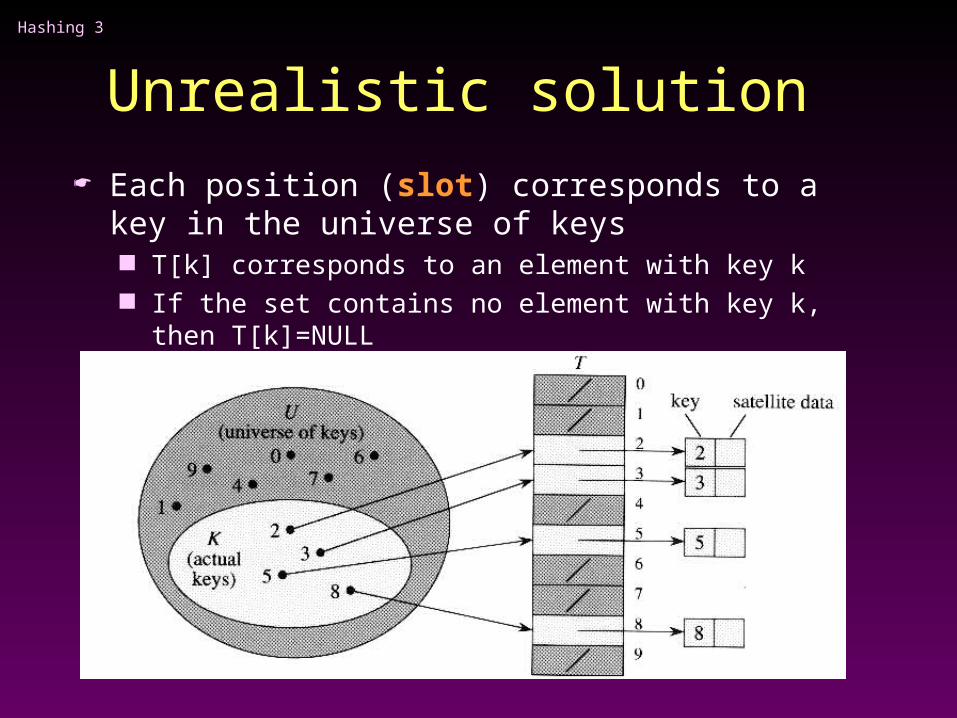
Unrealistic solution Each position (slot) corresponds to a key in the

universe of keys T[k] corresponds to an element with key k If the set contains no element with key k, then T[k]=NULL

Hashing 4

Unrealistic solution

insert, delete and find all take O(1) (worst-case) time

Problem: The scheme wastes too much space if the

universe is too large compared with the actual number of elements to be stored.

E.g. student IDs are 8-digit integers, so the universe size is 108, but we only have about 7000 students

Hashing 5

Hashing

Usually, m << N.

h(Ki) = an integer in [0, …, m-1] called the hash value of Ki

Hashing 6

Example applications Compilers use hash tables (symbol table) to keep

track of declared variables.

On-line spell checkers. After prehashing the entire dictionary, one can check each word in constant time and print out the misspelled word in order of their appearance in the document.

Useful in applications when the input keys come in sorted order. This is a bad case for binary search tree. AVL tree and B+-tree are harder to implement and they are not necessarily more efficient.

Hashing 7

Hashing With hashing, an element of key k is stored in T[h(k)]

h: hash function maps the universe U of keys into the slots of a hash table

T[0,1,...,m-1] an element of key k hashes to slot h(k) h(k) is the hash value of key k

Hashing 8

Hashing

Problem: collision two keys may hash to the same slot can we ensure that any two distinct keys get

different cells? No, if |U|>m, where m is the size of the hash table

Design a good hash function that is fast to compute and can minimize the number of collisions

Design a method to resolve the collisions when they occur

Hashing 9

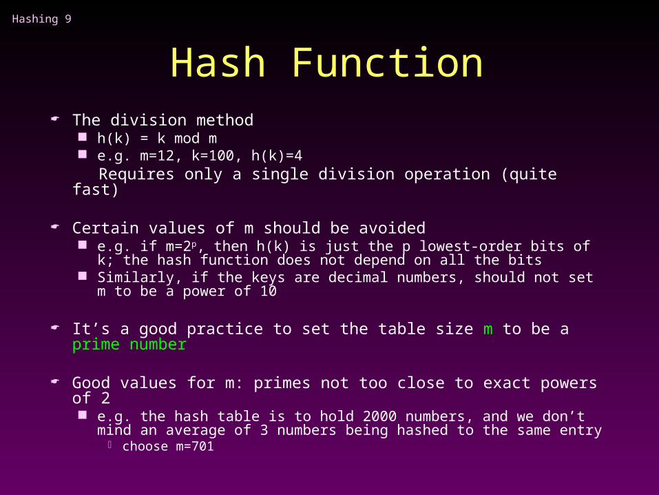
Hash Function The division method

h(k) = k mod m e.g. m=12, k=100, h(k)=4

Requires only a single division operation (quite fast)

Certain values of m should be avoided e.g. if m=2p, then h(k) is just the p lowest-order bits of k; the hash

function does not depend on all the bits Similarly, if the keys are decimal numbers, should not set m to be a

power of 10

It’s a good practice to set the table size m to be a prime number

Good values for m: primes not too close to exact powers of 2 e.g. the hash table is to hold 2000 numbers, and we don’t mind an

average of 3 numbers being hashed to the same entry choose m=701

Hashing 10

Hash Function... Can the keys be strings? Most hash functions assume that the keys are natural

numbers if keys are not natural numbers, a way must be found to

interpret them as natural numbers

Method 1 Add up the ASCII values of the characters in the string Problems:

Different permutations of the same set of characters would have the same hash value

If the table size is large, the keys are not distribute well. e.g. Suppose m=10007 and all the keys are eight or fewer characters long. Since ASCII value <= 127, the hash function can only assume values between 0 and 127*8=1016

Hashing 11

Hash Function... Method 2

If the first 3 characters are random and the table size is 10,0007 => a reasonably equitable distribution

Problem English is not random Only 28 percent of the table can actually be hashed to (assuming a table

size of 10,007)

Method 3 computes involves all characters in the key and be expected to distribute well

1

037*]1[

KeySize

i

iiKeySizeKey

272a,…,z and space

Hashing 12

Collision Handling: (1) Separate Chaining

Instead of a hash table, we use a table of linked list keep a linked list of keys that hash to the same value

h(K) = K mod 10

Hashing 13

Separate Chaining

To insert a key K Compute h(K) to determine which list to traverse If T[h(K)] contains a null pointer, initiatize this entry

to point to a linked list that contains K alone. If T[h(K)] is a non-empty list, we add K at the

beginning of this list.

To delete a key K compute h(K), then search for K within the list at

T[h(K)]. Delete K if it is found.

Hashing 14

Separate Chaining Assume that we will be storing n keys. Then we

should make m the next larger prime number. If the hash function works well, the number of keys in each linked list will be a small constant.

Therefore, we expect that each search, insertion, and deletion can be done in constant time.

Disadvantage: Memory allocation in linked list manipulation will slow down the program.

Advantage: deletion is easy.

Hashing 15

Collision Handling:(2) Open Addressing

Open addressing: relocate the key K to be inserted if it collides with an existing

key. That is, we store K at an entry different from T[h(K)].

Two issues arise what is the relocation scheme? how to search for K later?

Three common methods for resolving a collision in open addressing Linear probing Quadratic probing Double hashing

Hashing 16

Open Addressing To insert a key K, compute h0(K). If T[h0(K)] is empty,

insert it there. If collision occurs, probe alternative cell h1(K), h2(K), .... until an empty cell is found.

hi(K) = (hash(K) + f(i)) mod m, with f(0) = 0 f: collision resolution strategy

Hashing 17

Linear Probing f(i) =i

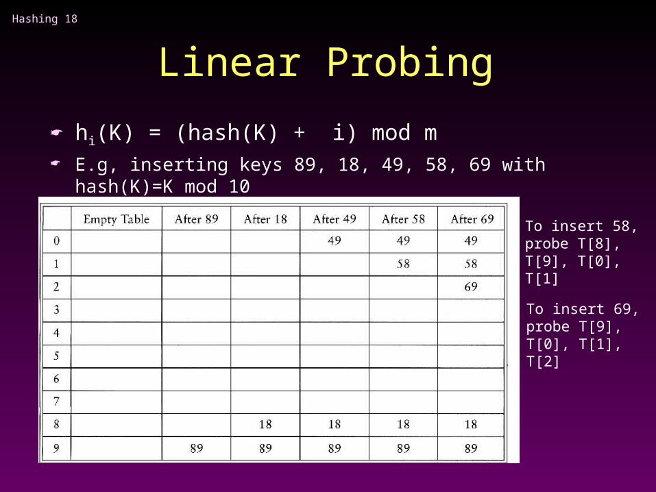
cells are probed sequentially (with wraparound) hi(K) = (hash(K) + i) mod m

Insertion: Let K be the new key to be inserted. We compute hash(K)

For i = 0 to m-1 compute L = ( hash(K) + I ) mod m T[L] is empty, then we put K there and stop.

If we cannot find an empty entry to put K, it means that the table is full and we should report an error.

Hashing 18

Linear Probing

hi(K) = (hash(K) + i) mod m E.g, inserting keys 89, 18, 49, 58, 69 with hash(K)=K mod 10

To insert 58, probe T[8], T[9], T[0], T[1]

To insert 69, probe T[9], T[0], T[1], T[2]

Hashing 19

Primary Clustering We call a block of contiguously occupied table entries a cluster

On the average, when we insert a new key K, we may hit the middle of a cluster. Therefore, the time to insert K would be proportional to half the size of a cluster. That is, the larger the cluster, the slower the performance.

Linear probing has the following disadvantages: Once h(K) falls into a cluster, this cluster will definitely grow in size by one.

Thus, this may worsen the performance of insertion in the future.

If two cluster are only separated by one entry, then inserting one key into a cluster can merge the two clusters together. Thus, the cluster size can increase drastically by a single insertion. This means that the performance of insertion can deteriorate drastically after a single insertion.

Large clusters are easy targets for collisions.

Hashing 20

Quadratic Probing f(i) = i2

hi(K) = ( hash(K) + i2 ) mod m E.g., inserting keys 89, 18, 49, 58, 69 with hash(K) = K mod 10

To insert 58, probe T[8], T[9], T[(8+4) mod 10]

To insert 69, probe T[9], T[(9+1) mod 10], T[(9+4) mod 10]

Hashing 21

Quadratic Probing Two keys with different home positions will have different probe

sequences e.g. m=101, h(k1)=30, h(k2)=29 probe sequence for k1: 30,30+1, 30+4, 30+9 probe sequence for k2: 29, 29+1, 29+4, 29+9

If the table size is prime, then a new key can always be inserted if the table is at least half empty (see proof in text book)

Secondary clustering Keys that hash to the same home position will probe the same

alternative cells Simulation results suggest that it generally causes less than an extra

half probe per search To avoid secondary clustering, the probe sequence need to be a

function of the original key value, not the home position

Hashing 22

Double Hashing To alleviate the problem of clustering, the sequence of

probes for a key should be independent of its primary position => use two hash functions: hash() and hash2()

f(i) = i * hash2(K) E.g. hash2(K) = R - (K mod R), with R is a prime smaller than

m

Hashing 23

Double Hashing hi(K) = ( hash(K) + f(i) ) mod m; hash(K) = K mod m

f(i) = i * hash2(K); hash2(K) = R - (K mod R), Example: m=10, R = 7 and insert keys 89, 18, 49, 58, 69

To insert 49, hash2(49)=7, 2nd probe is T[(9+7) mod 10]

To insert 58, hash2(58)=5, 2nd probe is T[(8+5) mod 10]

To insert 69, hash2(69)=1, 2nd probe is T[(9+1) mod 10]

Hashing 24

Choice of hash2() Hash2() must never evaluate to zero

For any key K, hash2(K) must be relatively prime to the table size m. Otherwise, we will only be able to examine a fraction of the table entries. E.g.,if hash(K) = 0 and hash2(K) = m/2, then we can only examine

the entries T[0], T[m/2], and nothing else!

One solution is to make m prime, and choose R to be a prime smaller than m, and set

hash2(K) = R – (K mod R)

Quadratic probing, however, does not require the use of a second hash function likely to be simpler and faster in practice

Hashing 25

Deletion in open addressing Actual deletion cannot be performed in open

addressing hash tables otherwise this will isolate records further down the probe

sequence

Solution: Add an extra bit to each table entry, and mark a deleted slot by storing a special value DELETED (tombstone)