arX

iv:0

901.

4007

v1 [

stat

.AP]

26

Jan

2009

The Annals of Applied Statistics

2008, Vol. 2, No. 4, 1332–1359DOI: 10.1214/08-AOAS184c© Institute of Mathematical Statistics, 2008

EMPIRICAL NULL AND FALSE DISCOVERY RATEINFERENCE FOR EXPONENTIAL FAMILIES

By Armin Schwartzman1

Harvard School of Public Health and Dana-Farber Cancer Institute

In large scale multiple testing, the use of an empirical null distri-bution rather than the theoretical null distribution can be critical forcorrect inference. This paper proposes a “mode matching” method forfitting an empirical null when the theoretical null belongs to any ex-ponential family. Based on the central matching method for z-scores,mode matching estimates the null density by fitting an appropriateexponential family to the histogram of the test statistics by Pois-son regression in a region surrounding the mode. The empirical nullestimate is then used to estimate local and tail false discovery rate(FDR) for inference. Delta-method covariance formulas and approx-imate asymptotic bias formulas are provided, as well as simulationstudies of the effect of the tuning parameters of the procedure onthe bias-variance trade-off. The standard FDR estimates are foundto be biased down at the far tails. Correlation between test statis-tics is taken into account in the covariance estimates, providing ageneralization of Efron’s “wing function” for exponential families.Applications with χ2 statistics are shown in a family-based genome-wide association study from the Framingham Heart Study and ananatomical brain imaging study of dyslexia in children.

1. Introduction. In large-scale multiple testing problems, the observeddistribution of the test statistics often does not accurately match the the-oretical null distribution [Efron et al. (2001), Efron (2004, 2005b)]. In suchcases, the use of an empirical null distribution, estimated from the data it-self, can be critical for making correct inferences. Previous empirical nullmethods [Efron (2004, 2007b), Jin and Cai (2007), Efron (2008)] have fo-cused on situations where the theoretical distribution of the test statis-tics is N(0,1) or t, typically found, for example, in two-group microarray

Received May 2008; revised May 2008.1Supported in part by a William R. and Sara Hart Kimball Stanford Graduate Fellow-

ship.Key words and phrases. Multiple testing, multiple comparisons, mixture model, Pois-

son regression, genome-wide association, brain imaging.

This is an electronic reprint of the original article published by theInstitute of Mathematical Statistics in The Annals of Applied Statistics,2008, Vol. 2, No. 4, 1332–1359. This reprint differs from the original in paginationand typographic detail.

1

2 A. SCHWARTZMAN

gene expression studies. Other large-scale multiple testing problems presenttheoretical null distributions that are not normal or t. For instance, χ2

tests are commonplace in the analysis of genome-wide association studiesbased on single nucleotide polymorphisms (SNPs) [Van Steen et al. (2005),Kong, Pu and Park (2006)], while multivariate F tests appear in voxel-basedanalyses of brain imaging studies [Everitt and Bullmore (1999), Schwartz-man, Dougherty and Taylor (2005), Lee et al. (2007), Schwartzman et al.(2008b, 2008a)].

This paper extends the scope of the empirical null to distributions thatbelong to general exponential families, treating the normal and χ2, as well astheir counterparts t and F , as special cases. This extension allows the empir-ical null to be flexibly chosen as a parametric exponential family version ofthe theoretical null. For example, where the theoretical null N(0,1) may bereplaced by an empirical null N(µ,σ2) with arbitrary mean µ and varianceσ2, a theoretical null χ2(ν0) with fixed ν0 degrees of freedom may be replacedby a scaled χ2 density (i.e., gamma) with arbitrary scaling factor a and arbi-trary number of degrees of freedom ν [Schwartzman, Dougherty and Taylor(2008a)].

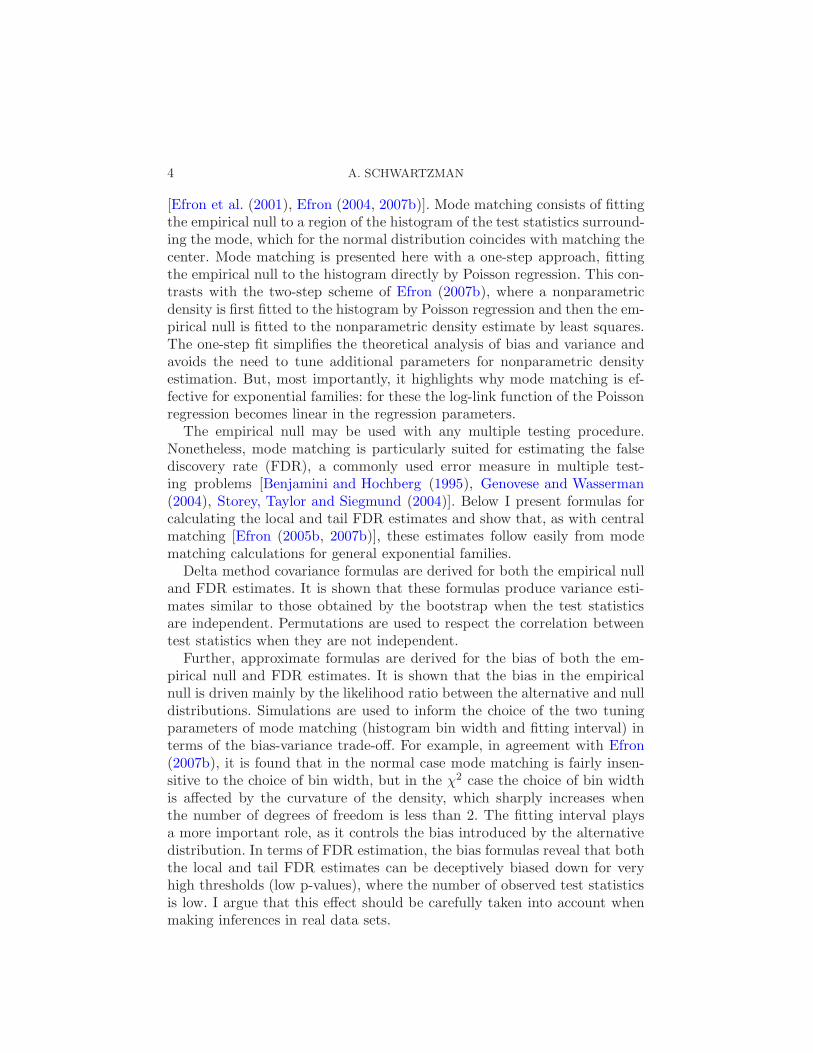
As a first data example, consider the following family-based study ofgenome-wide association between genetic variants and obesity based onthe Framingham Heart Study (FHS) [Herbert et al. (2006)]. Briefly, geneticmarkers were obtained by genotyping 1400 probands from the family-plateson an Affymetrix 100K SNP-chip containing 116,204 SNPs. Each SNP wastested for association with four body-mass index measurements at exams 1,2, 3 and 4 using the multivariate FBAT-GEE statistic [Lange et al. (2003)].Excluding SNPs for which the number of informative families was less than20, a total of 95,810 test statistics were generated with theoretical null χ2(4).Figure 1(a) shows that the histogram of the test statistics is not as wellmatched by the theoretical null χ2(4) (see zoom-in) as by the empirical null,a scaled χ2 with 4.27 d.f. and scaling factor 0.95. The mismatch between thehistogram and the theoretical null can be seen better in the p-value scalein Figure 1(b). The histogram of p-values according to the empirical null iscloser to a uniform distribution than that according to the theoretical null.

A second example where the effect is more dramatic is the brain imag-ing study analyzed in Schwartzman, Dougherty and Taylor (2008a). In brief,diffusion tensor imaging (DTI) scans were taken of 6 dyslexic and 6 nondyslexicchildren. After spatial registration, at each of 20,931 voxels a directional teststatistic was computed for testing whether the first eigenvector of the meandiffusion tensor has the same 3D spatial orientation in both groups. Thescores for each voxel were obtained by a quantile transformation from thetheoretical null model F (2,20) to χ2(2). Figure 2(a) shows a histogram ofthe 20,931 χ2-scores. The data histogram is not well matched by the theo-retical null χ2(2) but is better described by the empirical null, a χ2 with 1.82

EMPIRICAL NULL FOR EXPONENTIAL FAMILIES 3

d.f. This is better seen in Figure 2(b). For p-values that are most likely null,say, higher than 0.1, the theoretical null produces a histogram that can behardly explained by a uniform distribution. In contrast, the empirical nullproduces a histogram that is mostly uniform in that range. Moreover, thenumber of voxels with low p-values (less than 0.05) is higher according tothe empirical null, indicating a gain in statistical power. Schwartzman et al.(2008b) show other examples of voxel-based analyses in brain imaging withnormal and χ2 statistics where the empirical null is necessary for correctinference.

The proposed method for fitting the empirical null, which I call ‘modematching’, is a generalization of the central matching method for z-scores

Fig. 1. SNP example: (a) Histogram of the test statistics (light gray). Superimposed den-sities are the theoretical null χ2(4) (dashed) and the empirical null (solid) with pointwisestandard 95% CIs. The histogram of the estimated alternative component and correspond-ing upper standard CI are shown in inverted scale. Inlet plot is a zoom-in. (b) Histogramof p-values according to the theoretical null (light gray) and the empirical null (black).

Fig. 2. DTI example: (a) Histogram of the χ2-scores (light gray). Superimposed densitiesare the theoretical null χ2(2) (dashed) and the empirical null (solid) with pointwise stan-dard 95% CIs. The histogram of the estimated alternative component and correspondingupper standard CI are shown in inverted scale. (b) Histogram of p-values according to thetheoretical null (light gray) and the empirical null (black).

4 A. SCHWARTZMAN

[Efron et al. (2001), Efron (2004, 2007b)]. Mode matching consists of fittingthe empirical null to a region of the histogram of the test statistics surround-ing the mode, which for the normal distribution coincides with matching thecenter. Mode matching is presented here with a one-step approach, fittingthe empirical null to the histogram directly by Poisson regression. This con-trasts with the two-step scheme of Efron (2007b), where a nonparametricdensity is first fitted to the histogram by Poisson regression and then the em-pirical null is fitted to the nonparametric density estimate by least squares.The one-step fit simplifies the theoretical analysis of bias and variance andavoids the need to tune additional parameters for nonparametric densityestimation. But, most importantly, it highlights why mode matching is ef-fective for exponential families: for these the log-link function of the Poissonregression becomes linear in the regression parameters.

The empirical null may be used with any multiple testing procedure.Nonetheless, mode matching is particularly suited for estimating the falsediscovery rate (FDR), a commonly used error measure in multiple test-ing problems [Benjamini and Hochberg (1995), Genovese and Wasserman(2004), Storey, Taylor and Siegmund (2004)]. Below I present formulas forcalculating the local and tail FDR estimates and show that, as with centralmatching [Efron (2005b, 2007b)], these estimates follow easily from modematching calculations for general exponential families.

Delta method covariance formulas are derived for both the empirical nulland FDR estimates. It is shown that these formulas produce variance esti-mates similar to those obtained by the bootstrap when the test statisticsare independent. Permutations are used to respect the correlation betweentest statistics when they are not independent.

Further, approximate formulas are derived for the bias of both the em-pirical null and FDR estimates. It is shown that the bias in the empiricalnull is driven mainly by the likelihood ratio between the alternative and nulldistributions. Simulations are used to inform the choice of the two tuningparameters of mode matching (histogram bin width and fitting interval) interms of the bias-variance trade-off. For example, in agreement with Efron(2007b), it is found that in the normal case mode matching is fairly insen-sitive to the choice of bin width, but in the χ2 case the choice of bin widthis affected by the curvature of the density, which sharply increases whenthe number of degrees of freedom is less than 2. The fitting interval playsa more important role, as it controls the bias introduced by the alternativedistribution. In terms of FDR estimation, the bias formulas reveal that boththe local and tail FDR estimates can be deceptively biased down for veryhigh thresholds (low p-values), where the number of observed test statisticsis low. I argue that this effect should be carefully taken into account whenmaking inferences in real data sets.

EMPIRICAL NULL FOR EXPONENTIAL FAMILIES 5

The effect of dependence in the covariance of the empirical null and FDRestimates is explained in terms of the empirical distribution of pairwise cor-relation between test statistics in a way similar to Efron (2007a). I showthat Efron’s enigmatic “wing function” is a special case of the large familyof Lancaster polynomials of bivariate exponential families, which reduces tothe Hermite polynomials in the normal case and to the Laguerre polynomialsin the χ2 case.

Mode matching is both computationally efficient and easy to implementbecause it is based on Poisson regression, for which software is widely avail-able. The analysis is demonstrated in both the DTI and SNP examplesintroduced above. The SNP example demonstrates the bias, while the DTIexample demonstrates the effect of correlation. While both examples have χ2

null distributions, I emphasize that the methodology is designed for generalexponential families. Specific procedures and simulation results are shownfor both the normal and χ2 cases.

2. Mode matching for exponential families.

2.1. Setup. Let T1, . . . , TN be a large collection of N test statistics. Thetwo-class mixture model [Efron et al. (2001), Storey (2003), Efron (2004,2007b) Sun and Cai (2007)]

f(t) = p0f0(t) + (1− p0)fA(t)(1)

specifies that a fixed fraction p0 of the test statistics behave according to acommon null distribution with density f0(t). The other test statistics behaveaccording to alternative densities whose mixture is fA(t). The null densityf0(t) is assumed unimodal. The zero assumption, needed for identifiabilityof the model, is loosely defined by Efron as the condition that most of theprobability mass near the mode of f(t) is due to the null term p0f0(t), forexample, p0 > 0.9 (the effect of overlap between the null and alternativecomponents is discussed in Section 4). The objective of the empirical nullmethodology is to estimate p0 and f0 from T1, . . . , TN .

Mode matching begins by summarizing the data into a vector of histogramcounts y = (y1, . . . , yK)′ with yk =

∑Ni=1 1{Ti ∈Bk}, k = 1, . . . ,K, for K bins

Bk centered at t = (t1, . . . , tK)′. For simplicity, I assume all bins have thesame width ∆, although this is not crucial. If the test statistics are inde-pendent, then, given N , the counts y follow a multinomial distribution withprobabilities π = (π1, . . . , πK)′, πk = P (Ti ∈ Bk). By the Taylor expansionaround tk,

πk =

∫

Bk

f(t)dt=∆f(tk) +∆3

24f ′′(tk) + · · · ≈∆f(tk).(2)

6 A. SCHWARTZMAN

The approximation is valid if the bin width ∆ is small and the marginaldensity f(t) is smooth (the effect of curvature is discussed in Section 4).Thus, for large N , the scaled histogram

f(t) =y

N∆(3)

is a nearly unbiased estimate of f(t) at the bin centers t.The next step is to choose a closed interval S0 where the zero assumption

may hold. S0 is the union of K0 <K consecutive bins containing the mode off(t). For example, for a two-sided test with theoretical null N(0,1), S0 maybe of the form S0 = [tmin, tmax], while for a one-sided test with theoreticalnull χ2, S0 may be of the form S0 = [0, tmax]. Within S0, the zero assumptionmakes (3) an estimate of the scaled null p0f0(t) in (1), with additional bias(1− p0)fA(t).

Suppose f0(t) is a parametric density. Instead of maximizing the multino-mial likelihood given y, mode matching uses, almost equivalently, Poissonregression. The idea, also called Lindsey’s method [Efron and Tibshirani(1996), Efron (2007b)], is to consider the number of tests N as a Poissonvariable N ∼ Po(γ). If the test statistics are independent, then the histogramcounts become independent Poisson variables yk ∼ Po(λk) with λk = γπk.If N is large, this is essentially the same as the usual Poisson approxi-mation to the multinomial. Using (2), we have λk = γπk ≈ γ∆f(tk). Thus,within S0, the zero assumption leads to the general Poisson regression modelyk ∼ Po(λk) with

λk ≈ γ∆p0f0(tk), tk ∈ S0,(4)

where γ is replaced by its MLE, the observed count N .

2.2. Exponential families. Since the link function for Poisson regressionis logarithmic, the precise parametric form of f0(t) needed to make log(λk)in (4) linear in the parameters is an exponential family. Let

f0(t) = g0(t) exp(x(t)′η− ψ(η)),(5)

where g0(t) is the carrier density, η is the vector of canonical parameters,x(t) is the sufficient vector and ψ(η) is the cumulant generating function.Replacing in (4) gives the linear Poisson regression model yk ∼ Po(λk) with

log(λk) = x(tk)′η+C + hk,(6)

where the entries of x(tk) play the role of predictors,

C =C(η) = log p0 −ψ(η)(7)

is a constant intercept, and hk = log(N∆g0(tk)) is an offset. It is convenientto write model (6) in vector form as

log(λ) =Xη+ + h,(8)

EMPIRICAL NULL FOR EXPONENTIAL FAMILIES 7

where λ = (λ1, . . . , λK)′, η+ = (C,η′)′ is the augmented parameter vec-tor, the design matrix X has rows (1,x(tk)

′) for k = 1, . . . ,K, and h =(h1, . . . , hK)′. The fit is restricted to the interval S0 by providing the Pois-son regression algorithm with an external set of weights w = (w1, . . . ,wK)′,where wk is equal to 1 or 0 according to whether tk is in S0 or not. Forlater use, define the diagonal matrix W with diagonal equal to w (not to beconfused with the weighting matrix used internally in the iterative solvingof the Poisson regression).

Solving (8) gives estimates η+ = (C, η)′, which include the empirical nullparameter estimates η. From these, an estimate of the null probability p0is also obtained using (7) as p0 = exp(C + ψ(η)). Notice that p0 is notconstrained to be less than or equal to 1. The predicted histogram countsλ=N∆f0(t) = y = (y1, . . . , yK)′ corresponding to the empirical null for allbins (not just within S0) are

y = exp(Xη+ +h).(9)

As a result, the predicted histogram counts corresponding to the alternativecomponent in (1) are

N∆(1− p0)fA(t) =N∆(f(t)− p0f0(t)) = y− y.(10)

Empirical null densities are more naturally specified using the usual pa-rameters of the distribution rather than the canonical ones. When the the-oretical null is N(0,1), the empirical null is N(µ,σ2) with θ = (µ,σ2)′

[Efron (2004, 2007b)] [t-statistics are handled by a quantile transformationto N(0,1)]. When the theoretical null is χ2 with ν0 d.f., an appropriate em-pirical null is a scaled χ2 with ν d.f. and scaling factor a, denoted aχ2(ν),with density

f0(t) =1

(2a)ν/2Γ(ν/2)e−t/(2a)tν/2−1,(11)

where θ = (a, ν)′ [Schwartzman, Dougherty and Taylor (2008a)]. This is thesame as a gamma density with shape parameter ν/2 and scaling parameter2a, but using the χ2 notation helps keep the connection to the theoreticalnull. F -statistics are handled by a quantile transformation to χ2 with thesame numerator number of degrees of freedom.

Let θ = θ(η) denote the vector of usual parameters as in the normaland χ2 examples above. Let θ+ = (log p0,θ

′)′ be the augmented parame-

ter vector. The MLE of θ+ is θ+ = (log p0,θ(η)′)′. The derivation of these

parameter estimates from the canonical parameter estimates for both thenormal and χ2 cases is worked out in Appendix A.

Other distributions are treated in a similar way. For p-values, whose the-oretical null is uniform, the empirical null may be a beta distribution with

8 A. SCHWARTZMAN

fitting interval S0 = [tmin,1]. If the theoretical null is a discrete exponen-tial family (e.g., binomial, Poisson, negative binomial), the mode matchingprocedure is the same as above except that the bins width ∆ = 1 is auto-matically set by the discrete nature of the distribution, making equations(2) and (4) exact rather than approximate.

2.3. Exponential subfamilies. In some cases, one may want to adjustonly some of the parameters in (5) and leave the others fixed as prescribedby the theoretical null. For instance, the microarray analysis examples inEfron (2007b) suggest the empirical null N(0, σ2), while in some fMRIstudies involving z-scores, an appropriate empirical null may be N(µ,1)[Ghahremani and Taylor (2005)]. If fixing some parameters results in an-other lower dimensional exponential family, then the procedure is similarto the one above after the canonical parameters have been redefined. Letη+ = (C,η′

1,η′

2)′, where η1 is the vector of canonical parameters to be es-

timated and η2 is the vector of parameters whose values are fixed. LetX = (1K ,X1,X2) be the corresponding split of the design matrix, where1K indicates a column of K ones. The regression equation (8) becomes

log(λ) = 1KC +X1η1 + (X2η2 + h)(12)

and is solved as before, except that the fixed term X2η2 is absorbed intothe offset in parenthesis. The specific exponential subfamilies of the normaland χ2 cases are worked out in detail in Appendix A.

The simplest restricted case is where one believes the theoretical null andno adjustment of parameters is necessary, except for p0 [Efron (2004)]. Inthat case, only the intercept C needs to be estimated in (12), treating all the

other terms as offset. The estimate of p0 is then given by p0 = exp(C+ψ(η)).Notice that, for the regression (12) to remain linear, p0 cannot be fixed apriori.

2.4. Covariance estimates. Covariance estimates for the empirical nullparameter estimates η+ can be obtained by the delta method in a waysimilar to Efron (2005b). For this we first need an estimate of the covarianceof y. As noted by Efron and Tibshirani (1996), there are two such estimates.The Poisson regression regards the observations yk as independent, so itsinfluence function is determined by the covariance estimate cov(y) = V =Diag(y), a K ×K diagonal matrix with diagonal entries yk. On the otherhand, the true covariance of y depends on the dependence structure of thetest statistics.

Suppose first the test statistics are independent. Then conditional on N ,the yk are multinomial, for which an appropriate covariance estimate is

V N =Diag(y)− yy′/N.(13)

EMPIRICAL NULL FOR EXPONENTIAL FAMILIES 9

Proposition 1. Let ψ(η) and θ(η) denote the derivatives of ψ and θ

with respect to η evaluated at η. The delta method covariance estimates ofη+ and θ+ are respectively

cov(η+) = (X ′WVX)−1X ′WV NWX(X ′WVX)−1(14)

cov(θ+) = D cov(η+)D′

, D =

(1 ψ(η)′

0 θ(η)′

).(15)

Proposition 2. The delta method covariance estimate of the empiricalnull fits (9) and the empirical alternative component (10) are respectively

cov(y) = (V Dy)V N (V Dy)′ and cov(y − y) = (I − V Dy)V N (I − V Dy)

′,where Dy = ∂(log y)/∂y′ is given by

Dy =X(X ′WVX)−1X ′W .(16)

The above covariance estimates become more accurate as N increases.If the test statistics are mildly correlated, the Poisson regression scheme

may still be used to fit the empirical null, but the covariance estimates needto change. In this case, the delta-method covariance formulas in Propositions1 and 2 are applied with V N replaced by a covariance estimate other than(13) that reflects the correlation between the bin counts. This is illustratedbelow in the DTI example using permutations. Alternatively, one may fit theempirical null including an overdispersion parameter in the Poisson regres-sion. The overdispersion parameter φ is estimated by the quasi-likelihoodMLE φ = (1/K)

∑Kk=1(yk − λk)/λk. The Poisson regression fit is the same

as before, but the covariance estimates above are inflated by a factor φ.

2.5. The SNP data. Recall the SNP data set described in Section 1.The histogram in Figure 1(a) was constructed using bins of width ∆ = 0.1starting from zero. The empirical null was obtained using χ2 mode matching(Appendix A.2). The fitting interval was defined as S0 = [0,20], wide enoughto use most of the data without including the far tail region t > 20, wherediscoveries are likely to be made. These choices are discussed in Section 4.

The estimated parameters θ+ are listed in Table 1. Assuming indepen-dence of the test statistics, the associated standard errors (SE) were com-puted as the square root of the diagonal of (15) using the multinomial covari-ance (13). For comparison, I also used the bootstrap as follows. Again assum-ing independence, repeated resampling with replacement from {T1, . . . , TN}gave sets {T ∗

1 , . . . , T∗

N}, each leading to a parameter estimate (θ+)∗. The

bootstrap covariance estimate of θ+ was computed as the empirical covari-ance of the (θ+)∗ and the SEs as the square roots of the diagonal elements ofthis covariance. Notice that the delta-method SEs are only slightly smallerthan the bootstrap SEs.

10 A. SCHWARTZMAN

The CIs for a and ν do not include the theoretical values 1 and 4,indicating a significant departure from the theoretical null in both scal-ing and degrees of freedom. The CI for log(p0) includes 0. This does notprove that there are no significant SNPs, but it shows that the study maynot have enough power to discover them. The lower bound of the CI forlog(p0) suggests that the fraction of non-null SNPs may be as high as1− p0 ≈− log(p0) = 3.18× 10−5, which is about 3 SNPs out of N = 95,810.If instead of fitting the full empirical null, p0 is estimated alone believingthe theoretical null, the result is log(p0) = 1.24 × 10−4 with standard CI[1.96 × 10−5,2.28× 10−4]. The theoretical null does not admit an estimateof p0 that is less than 1, again indicating that the theoretical null is unsuit-able for this data.

The SEs in Table 1 are smaller than they would be if the dependence be-tween the test statistics were taken into account. I did not take into accountthe dependence because I did not have access to the original data but onlyto the FBAT test statistics. Given the complexity of the FBAT procedure,pairwise correlations between test statistics would be hard to estimate. Ithas been claimed that the SNPs in this dataset are not highly correlatedbecause of their widespread locations on the genome [Herbert et al. (2006)].One indication that the correlation may not have a large effect is that theestimated overdispersion from fitting the empirical null is φ= 1.090 (boot-strap SE = 0.066), not significantly larger than 1.

2.6. The DTI data. For the DTI data set, the histogram in Figure 2(a)was constructed using bins of width ∆ = 0.05 starting from zero and theempirical null was obtained using χ2 mode matching (Appendix A.2). Thefitting interval was defined as S0 = [0,4.5]. These choices are discussed inSection 4.

The estimated parameters θ+ are listed in Table 2. The associated SEswere computed as the square root of the diagonal of (15) using two different

values for V N . The naive estimate (column 4) assumes independence ofthe test statistics and uses the multinomial covariance (13). The estimate in

Table 1

SNP example: Theoretical null parameters (column 2) and empirical null estimates(column 3). Included are delta-method and bootstrap SE (columns 4 and 5) and standard

95% confidence intervals based on the delta-method SE (column 6)

θ+ Theory θ+ SE (15) Bootstrap SE 95% CI

log(p0) 0 7.49× 10−5 5.45× 10−5 5.89×10−5 [−3.18,18.2]× 10−5

a 1 0.9509 0.0046 0.0048 [0.9419,0.9600]ν 4 4.2675 0.0183 0.0199 [4.2316,4.3034]

EMPIRICAL NULL FOR EXPONENTIAL FAMILIES 11

column 5 replaces V N by a permutation estimate V P similar to the one usedby Efron (2007a), obtained as follows. In the original data, the group labelsof the two groups of 6 subjects were permuted, for a total of 924/2 = 462distinct permutations (the test statistics are symmetric, yielding the samevalue if the groups are swapped). For each permutation, the 20,931 teststatistics T ∗ were recomputed and a vector y∗ of histogram counts wasproduced. The permutation covariance estimate V P was computed as theempirical covariance of the y∗.

This permutation scheme relies on the subjects being independent butpreserves the correlation structure between the test statistics. While validityof the permutations requires the complete null assumption, removal of themean effects is difficult in this case because of the directional nature ofthe data. Yet, since p0 is close to 1, the null hypothesis is valid in mostvoxels and may be enough for the purposes of estimating global parameters,such as those of the empirical null. Table 2 shows that taking into accountcorrelation via the permutation scheme about doubles the naive SEs.

Based on the permutation SEs, the CI for a includes the theoretical value1, while the CI for ν does not include the theoretical value 2. This indicates asignificant departure from the theoretical null in degrees of freedom but notscaling. The CI for p0 does not include 1 and it is estimated that there are(1−p0)N = 745 non-null voxels in the data. The estimated overdispersion is

φ= 1.332 (permutation SE = 0.087), significantly larger than 1 as expectedfrom the dependence.

If instead of fitting the full empirical null, p0 is estimated alone believingthe theoretical null (blue curve in Figure 2), the result is p0 = 0.989 withnaive CI [0.984,0.994] and permutation CI [0.955,1.024]. The theoreticalnull not only provides a poor fit to the data but gives a higher estimate ofp0 than the empirical null, so one may say it is less powerful.

3. FDR inference.

Table 2

DTI example: Theoretical null parameters (column 2) and empirical null estimates(column 3). Included are delta-method SEs assuming independence (column 4) and using

permutations (column 5). The standard 95% confidence intervals are based on thepermutation SEs (column 6)

θ+ Theory θ+ SE (15), ind SE (15), perm 95% CI, perm

p0 1 0.964 0.0042 0.0080 [0.949,0.981]a 1 0.961 0.0225 0.0679 [0.828,1.094]ν 2 1.817 0.0223 0.0377 [1.743,1.891]

12 A. SCHWARTZMAN

3.1. FDR estimates. Mode matching is particularly convenient for FDRestimation, as FDR estimates follow immediately from the Poisson regressionfits (9). Let F (t) = p0F0(t)+ (1− p0)FA(t) be the cumulative version of (1).Recall that the local false discovery rate (fdr) and (positive) right-tail FDRare given respectively by

fdr(t) =p0f0(t)

f(t), FdrR(t) =

p0(1−F0(t))

1− F (t)=

∫∞

t fdr(u)f(u)du∫∞

t f(u)du(17)

[Efron et al. (2001), Efron (2004)]. Using (3) and (4), the local fdr at thebin centers tk is estimated by

fdr(tk) =p0f0(tk)

f(tk)=λk/(N∆)

yk/(N∆)=ykyk,(18)

defined whenever yk > 0, or in vector form as

log fdr= log y − logy,(19)

where y is given by (9). In contrast to Efron (2007b), I estimate FdrR atthe bin centers tk based on the right side of (17) by

FdrR(tk) =(1/2)fdr(tk)f(tk) +

∑Kj=k+1 fdr(tj)f(tj)

(1/2)f (tk) +∑K

j=k+1 f(tj)(20)

=(1/2)yk +

∑Kj=k+1 yj

(1/2)yk +∑K

j=k+1 yj,

where (3) and (18) were used. This can be written in vector form as

log FdrR = log(Sy)− log(Sy),(21)

where S is an upper triangular matrix with entries 1/2 on the diagonal and1 above the diagonal. The estimate (21) is easy to analyze theoretically interms of bias (see Section 4). For the left tail FDR, definition (17) is changedto FdrL(t) = p0F0(t)/F (t) and is estimated similarly by

log FdrL = log(S′y)− log(S ′y),(22)

where S′ is the transpose of S, a lower triangular matrix with entries 1/2on the diagonal and 1 below the diagonal.

Proposition 3. (a) The delta method covariance estimate of the local

fdr (19) is cov(log fdr) =AV NA′, where A= ∂(log fdr)/∂y′ =Dy −V −1,V =Diag(y) and Dy is given by (16).

(b) The delta method covariance estimate of the right tail FDR (21)

is cov(log FdrR) = BV NB′, where B = ∂(log FdrR)/∂y′ = U

−1SV Dy −

U−1 and U =Diag(Sy), U =Diag(Sy). The formula for the left tail FDR(22) has the same form with S replaced by S′.

EMPIRICAL NULL FOR EXPONENTIAL FAMILIES 13

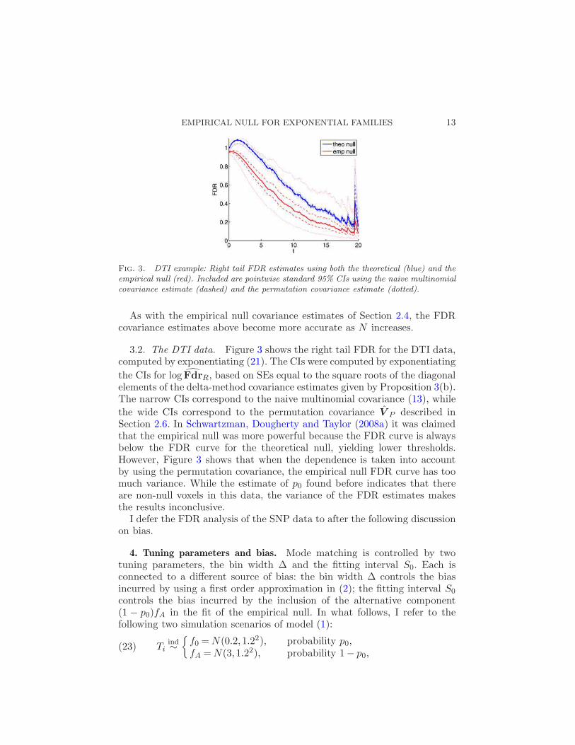
Fig. 3. DTI example: Right tail FDR estimates using both the theoretical (blue) and theempirical null (red). Included are pointwise standard 95% CIs using the naive multinomialcovariance estimate (dashed) and the permutation covariance estimate (dotted).

As with the empirical null covariance estimates of Section 2.4, the FDRcovariance estimates above become more accurate as N increases.

3.2. The DTI data. Figure 3 shows the right tail FDR for the DTI data,computed by exponentiating (21). The CIs were computed by exponentiating

the CIs for log FdrR, based on SEs equal to the square roots of the diagonalelements of the delta-method covariance estimates given by Proposition 3(b).The narrow CIs correspond to the naive multinomial covariance (13), while

the wide CIs correspond to the permutation covariance V P described inSection 2.6. In Schwartzman, Dougherty and Taylor (2008a) it was claimedthat the empirical null was more powerful because the FDR curve is alwaysbelow the FDR curve for the theoretical null, yielding lower thresholds.However, Figure 3 shows that when the dependence is taken into accountby using the permutation covariance, the empirical null FDR curve has toomuch variance. While the estimate of p0 found before indicates that thereare non-null voxels in this data, the variance of the FDR estimates makesthe results inconclusive.

I defer the FDR analysis of the SNP data to after the following discussionon bias.

4. Tuning parameters and bias. Mode matching is controlled by twotuning parameters, the bin width ∆ and the fitting interval S0. Each isconnected to a different source of bias: the bin width ∆ controls the biasincurred by using a first order approximation in (2); the fitting interval S0controls the bias incurred by the inclusion of the alternative component(1 − p0)fA in the fit of the empirical null. In what follows, I refer to thefollowing two simulation scenarios of model (1):

Tiind∼{f0 =N(0.2,1.22), probability p0,fA =N(3,1.22), probability 1− p0,

(23)

14 A. SCHWARTZMAN

Tiind∼{f0 = 0.8χ2(3), probability p0,fA = noncentralχ2(3, δ = 3), probability 1− p0,

(24)

where δ = 3 denotes the noncentrality parameter. The fitting interval is setto S0 = [0.2− t0,0.2 + t0] in the normal case and S0 = [0, t0] in the χ2 case,so that in both cases S0 is tuned by the single number t0.

4.1. The bin width. The first and smallest source of bias is the use of afirst order approximation in (2). Under the zero assumption, the error maybe approximated by the next expansion term

πk − f0(tk)∆≈ f ′′0 (tk)

24∆3, tk ∈ S0.(25)

As in nonparametric density estimation, bias is reduced by thinning the bins.However, the size of the bias depends also on the curvature of the empiricalnull. If f0 is N(µ,σ2), the largest curvature occurs at the mode µ, wheref ′′0 (µ) ≈ −0.4/σ3. Thus, the error (25) is bounded by 0.017∆3/σ3. This isabout 1.3×10−4 if ∆ = 0.2σ. If f0 is aχ

2(ν), the curvature depends stronglyon ν. For ν < 6 except ν = 2, the curvature is unbounded at t = 0, but itdecreases rapidly as t increases away from 0. For ν ≥ 2, more important isthe curvature at the mode, where most of the probability mass lays. Thiscurvature decreases rapidly as ν increases away from 2. For example, forν = 3, the curvature at the mode ν − 2 is f ′′0 (ν − 2)≈−0.12/a3 so the error(25) is bounded by 0.005∆3/a3. This is about 4× 10−5 if ∆ = 0.2a.

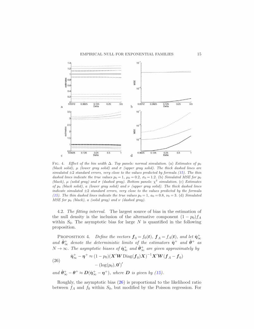
The effect of ∆ is illustrated in Figure 4. The plotted empirical null es-timates are averages over 100 simulated instances of models (23) and (24)with p0 = 1, N = 10,000, and fixed t0 = 1 in the normal case and t0 = 4 inthe χ2 case. In contrast to nonparametric density estimation, the varianceis remarkably insensitive to ∆. Within the plotted range, the variance issmallest for the smallest value of ∆. This is because, for fixed S0, a small∆ implies a large number of bins K = |S0|/∆ and thus a large number ofdesign points for the Poisson regression. Therefore, one may want the small-est possible ∆ as long as the number of counts yk within each bin in S0remains large, say, in the hundreds. Of course, this depends on the numberof tests N . A larger N allows a smaller ∆. The caveat is computational.A large number of bins K implies inverting large matrices in the fitting ofthe empirical null. For N = 10,000, based on Figure 4 and computationalconsiderations, ∆ = 0.05∼ 0.1 seems a reasonable choice for the normal andχ2(ν) with ν ≥ 2. If ν < 2, the curvature near t= 0 demands much smallervalues of ∆ to avoid substantial bias. For large ν, the increase in the ef-fective support of the density may require increasing ∆ in order to reducecomputations.

EMPIRICAL NULL FOR EXPONENTIAL FAMILIES 15

Fig. 4. Effect of the bin width ∆. Top panels: normal simulation. (a) Estimates of p0(black solid), µ (lower gray solid) and σ (upper gray solid). The thick dashed lines aresimulated ±2 standard errors, very close to the values predicted by formula (15). The thindashed lines indicate the true values p0 = 1, µ0 = 0.2, σ0 = 1.2. (b) Simulated MSE for p0(black), µ (solid gray) and σ (dashed gray). Bottom panels: χ2 simulation. (c) Estimatesof p0 (black solid), a (lower gray solid) and ν (upper gray solid). The thick dashed linesindicate simulated ±2 standard errors, very close to the values predicted by the formula(15). The thin dashed lines indicate the true values p0 = 1, a0 = 0.8, ν0 = 3. (d) SimulatedMSE for p0 (black), a (solid gray) and ν (dashed gray).

4.2. The fitting interval. The largest source of bias in the estimation ofthe null density is the inclusion of the alternative component (1 − p0)fAwithin S0. The asymptotic bias for large N is quantified in the followingproposition.

Proposition 4. Define the vectors f0 = f0(t), fA = fA(t), and let η+∞

and θ+∞

denote the deterministic limits of the estimators η+ and θ+ as

N →∞. The asymptotic biases of η+∞

and θ+∞

are given approximately by

η+∞

− η+ ≈ (1− p0)(X′W Diag(f0)X)−1

X ′W (fA − f0)(26)

− (log(p0),0′)′

and θ+∞

− θ+ ≈D(η+∞

− η+), where D is given by (15).

Roughly, the asymptotic bias (26) is proportional to the likelihood ratiobetween fA and f0 within S0, but modified by the Poisson regression. For

16 A. SCHWARTZMAN

Table 3

Asymptotic bias in the estimation of θ+. The limit θ+∞ = θ(η+

∞) was computed from thesolution to the limiting score equation (38)

Null θ+ θ+∞ θ

+∞ − θ+ Formula (26)

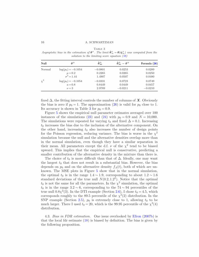
Normal log(p0)=−0.1054 −0.0801 0.0253 0.0289µ=0.2 0.2265 0.0265 0.0250σ2=1.44 1.4907 0.0507 0.0480

χ2 log(p0)=−0.1054 −0.0331 0.0723 0.0749a=0.8 0.8449 0.0449 0.0457ν=3 2.9789 −0.0211 −0.0210

fixed ∆, the fitting interval controls the number of columns of X . Obviouslythe bias is zero if p0 = 1. The approximation (26) is valid for p0 close to 1.Its accuracy is shown in Table 3 for p0 = 0.9.

Figure 5 shows the empirical null parameter estimates averaged over 100instances of the simulations (23) and (24) with p0 = 0.9 and N = 10,000.The simulations were repeated for varying t0 and fixed ∆ = 0.1. Increasingt0 increases the bias due to the inclusion of the alternative component. Onthe other hand, increasing t0 also increases the number of design pointsfor the Poisson regression, reducing variance. The bias is worse in the χ2

simulation because the null and the alternative densities overlap more thanin the normal simulation, even though they have a similar separation intheir mean. All parameters except the d.f. ν of the χ2 tend to be biasedupward. This implies that the empirical null is conservative, predicting asmaller contribution of the alternative density in the mixture than there is.

The choice of t0 is more difficult than that of ∆. Ideally, one may wantthe largest t0 that does not result in a substantial bias. However, the biasdepends on p0 and on the alternative density fA(t), both of which are un-known. The MSE plots in Figure 5 show that in the normal simulation,the optimal t0 is in the range 1.4 ∼ 1.9, corresponding to about 1.2 ∼ 1.6standard deviations of the true null N(0.2,1.22). Notice that the optimalt0 is not the same for all the parameters. In the χ2 simulation, the optimalt0 is in the range 3.2 ∼ 6, corresponding to the 74 ∼ 94 percentiles of thetrue null 0.8χ2(3). In the DTI example (Section 2.6), I chose t0 = 4.5, whichcorresponds roughly to the 89.5 percentile of the χ2(2) distribution. In theSNP example (Section 2.5), p0 is extremely close to 1, allowing t0 to bemuch larger. There I used t0 = 20, which is the 99.95 percentile of the χ2(4)distribution.

4.3. Bias in FDR estimation. One issue overlooked by Efron (2007b) isthat the local fdr estimate (18) is biased by definition. The bias is given bythe following proposition.

EMPIRICAL NULL FOR EXPONENTIAL FAMILIES 17

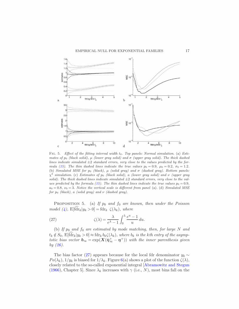
Fig. 5. Effect of the fitting interval width t0. Top panels: Normal simulation. (a) Esti-mates of p0 (black solid), µ (lower gray solid) and σ (upper gray solid). The thick dashedlines indicate simulated ±2 standard errors, very close to the values predicted by the for-mula (15). The thin dashed lines indicate the true values p0 = 0.9, µ0 = 0.2, σ0 = 1.2.(b) Simulated MSE for p0 (black), µ (solid gray) and σ (dashed gray). Bottom panels:χ2 simulation. (c) Estimates of p0 (black solid), a (lower gray solid) and ν (upper graysolid). The thick dashed lines indicate simulated ±2 standard errors, very close to the val-ues predicted by the formula (15). The thin dashed lines indicate the true values p0 = 0.9,a0 = 0.8, ν0 = 3. Notice the vertical scale is different from panel (a). (d) Simulated MSEfor p0 (black), a (solid gray) and ν (dashed gray).

Proposition 5. (a) If p0 and f0 are known, then under the Poisson

model (4), E[fdrk|yk > 0] = fdrk ζ(λk), where

ζ(λ) =λ

eλ − 1

∫ λ

0

eu − 1

udu.(27)

(b) If p0 and f0 are estimated by mode matching, then, for large N and

tk /∈ S0, E[fdrk|yk > 0]≈ fdrk bkζ(λk), where bk is the kth entry of the asymp-totic bias vector b∞ = exp(X(η+

∞− η+)) with the inner parenthesis given

by (26).

The bias factor (27) appears because for the local fdr denominator yk ∼Po(λk), 1/yk is biased for 1/λk. Figure 6(a) shows a plot of the function ζ(λ),closely related to the so-called exponential integral [Abramowitz and Stegun(1966), Chapter 5]. Since λk increases with γ (i.e., N ), most bins fall on the

18 A. SCHWARTZMAN

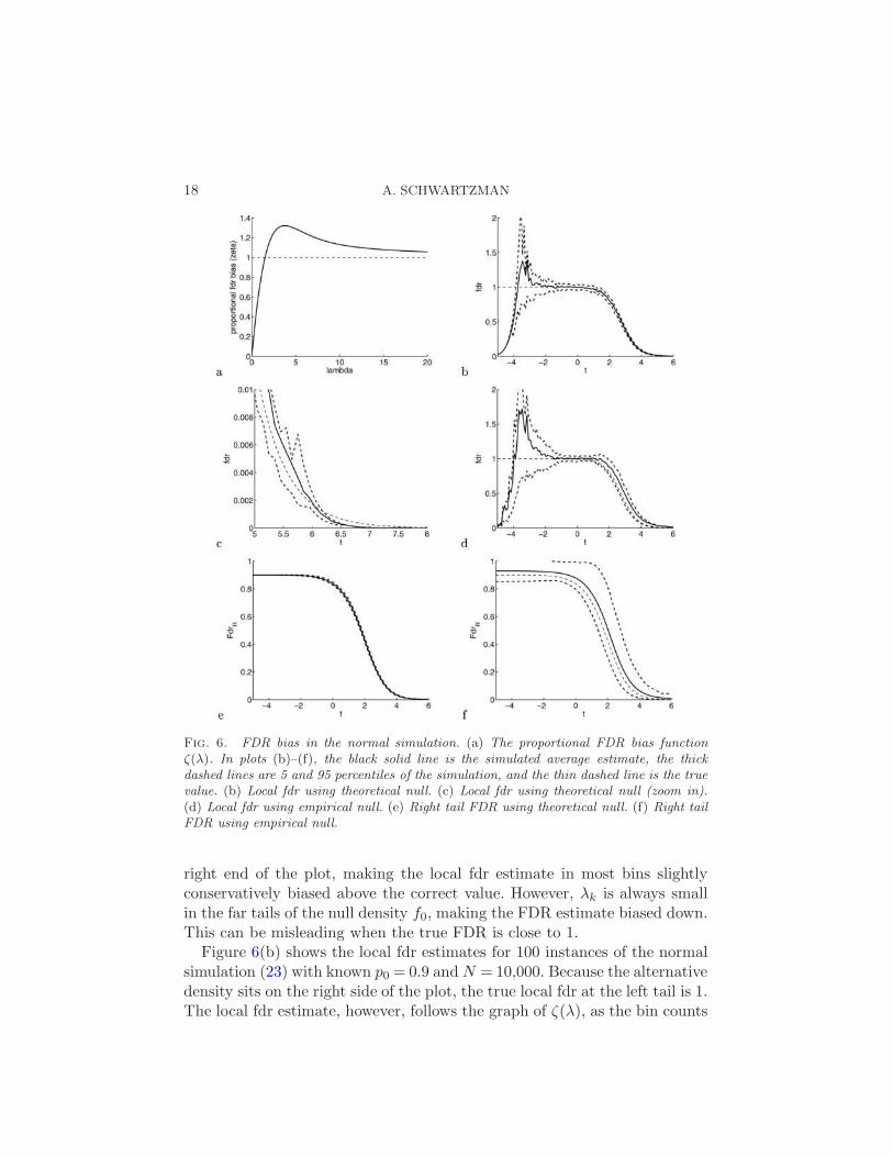
Fig. 6. FDR bias in the normal simulation. (a) The proportional FDR bias functionζ(λ). In plots (b)–(f), the black solid line is the simulated average estimate, the thickdashed lines are 5 and 95 percentiles of the simulation, and the thin dashed line is the truevalue. (b) Local fdr using theoretical null. (c) Local fdr using theoretical null (zoom in).(d) Local fdr using empirical null. (e) Right tail FDR using theoretical null. (f) Right tailFDR using empirical null.

right end of the plot, making the local fdr estimate in most bins slightlyconservatively biased above the correct value. However, λk is always smallin the far tails of the null density f0, making the FDR estimate biased down.This can be misleading when the true FDR is close to 1.

Figure 6(b) shows the local fdr estimates for 100 instances of the normalsimulation (23) with known p0 = 0.9 andN = 10,000. Because the alternativedensity sits on the right side of the plot, the true local fdr at the left tail is 1.The local fdr estimate, however, follows the graph of ζ(λ), as the bin counts

EMPIRICAL NULL FOR EXPONENTIAL FAMILIES 19

get smaller toward the left, with the variance proportional to that graph.Any particular realization of the FDR curve here may give the impressionthat there is something to discover at the left tail, while in reality there isnot. The zoom-in in panel c shows that the phenomenon still occurs in theright tail, as the average FDR estimate is first biased up with higher varianceand then dips below the truth as the bin counts get very small. This is notnoticeable in panel b because, by Proposition 5, the bias is proportional tothe true FDR, which is low in this region. When the empirical null is used,the additional bias and variance are visible in panel d. The additional biasis captured by the factor bk of Proposition 5(b), where the approximation isthe result of using the asymptotic bias for large N derived from Proposition4. Notice in Figure 6(d) that the bias is up, so the FDR estimates areconservative.

The tail FDR also suffers from a similar bias phenomenon, being sensitiveto small cumulative bin counts in the far tails. Following a similar argu-ment as in Proposition 5(a), when p0 and f0 are known, (20) says Fdrk =(Sλ0)k/(Sy)k, where the cumulative denominator yk/2+

∑Kl=k+1 yl behaves

similarly to a Poisson random variable with mean (Sλ)k = λk/2+∑K

l=k+1λl.

Therefore, E[Fdrk|yk > 0] = Fdrk ·E[(Sλ)k/(Sy)k|(Sy)k > 0], where the con-ditional expectation behaves approximately like ζ[(Sλ)k]. A simulation us-ing p0 = 1 (not shown) gives FDR curves that are very similar to those onthe left end of panels b and d. In Figure 6(e) (zoom-in not shown), the biasis visible but small because the FDR itself is low in the right tail. Panel fshows the increase in bias and variance when the empirical null is used.

The bias phenomenon does not contradict the results of Storey, Taylorand Siegmund (2004), which claim asymptotic unbiasedness of the tail FDRestimator. Consider a fixed bin k. As N increases, the expected bin count λkincreases and the operating point in Figure 6(a) moves to the right, makingthe FDR estimate asymptotically unbiased. The ζ(λ) phenomenon appealsto practical cases where N is large but finite, so that the bin counts at thetails are still small.

Efron (2004, 2007b) circumvented the bias problem by smoothing thehistogram with a spline fit. This helps because the compounding of data ateach bin pushes the operating point in the ζ(λ) graph [Figure 6(a)] to theright. However, smoothing introduces a bias of its own. Simulations usingsmoothing show that the resulting estimates at the far tails, especially whenp0 = 1, are not reliable, as they are very sensitive to the choice of knots orsmoothing bandwidth.

4.4. The SNP data. The FDR analysis is summarized in Figure 7. Here Ifocus on the local fdr, which in this case is more powerful than the tail FDR.The observed local fdr estimates (18) are compared to their expected value

20 A. SCHWARTZMAN

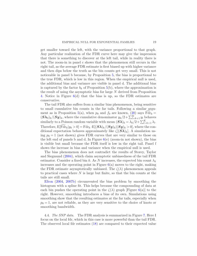
Fig. 7. SNP example: local fdr estimates using the empirical null. Top panel: full range.Bottom panel: zoom-in including standard 95% CIs. In both panels the dashed line is theexpectation of the local fdr estimate under the complete null.

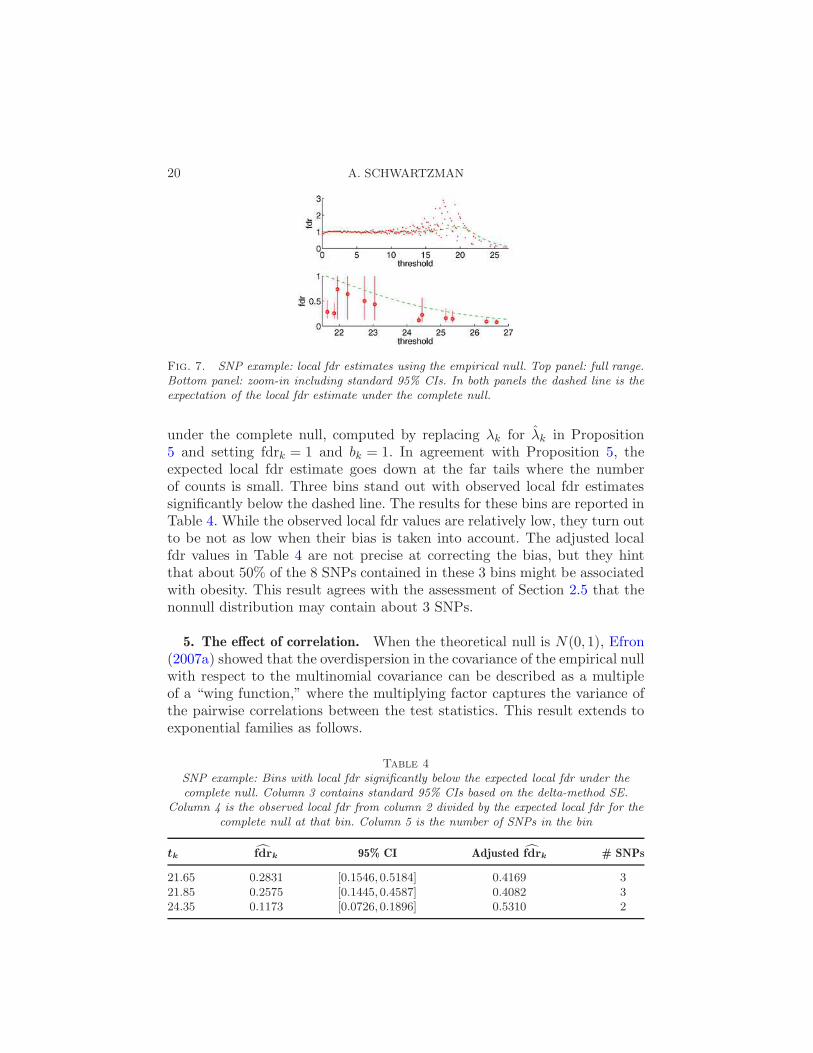
under the complete null, computed by replacing λk for λk in Proposition5 and setting fdrk = 1 and bk = 1. In agreement with Proposition 5, theexpected local fdr estimate goes down at the far tails where the numberof counts is small. Three bins stand out with observed local fdr estimatessignificantly below the dashed line. The results for these bins are reported inTable 4. While the observed local fdr values are relatively low, they turn outto be not as low when their bias is taken into account. The adjusted localfdr values in Table 4 are not precise at correcting the bias, but they hintthat about 50% of the 8 SNPs contained in these 3 bins might be associatedwith obesity. This result agrees with the assessment of Section 2.5 that thenonnull distribution may contain about 3 SNPs.

5. The effect of correlation. When the theoretical null is N(0,1), Efron(2007a) showed that the overdispersion in the covariance of the empirical nullwith respect to the multinomial covariance can be described as a multipleof a “wing function,” where the multiplying factor captures the variance ofthe pairwise correlations between the test statistics. This result extends toexponential families as follows.

Table 4

SNP example: Bins with local fdr significantly below the expected local fdr under thecomplete null. Column 3 contains standard 95% CIs based on the delta-method SE.

Column 4 is the observed local fdr from column 2 divided by the expected local fdr for thecomplete null at that bin. Column 5 is the number of SNPs in the bin

tk fdrk 95% CI Adjusted fdrk # SNPs

21.65 0.2831 [0.1546,0.5184] 0.4169 321.85 0.2575 [0.1445,0.4587] 0.4082 324.35 0.1173 [0.0726,0.1896] 0.5310 2

EMPIRICAL NULL FOR EXPONENTIAL FAMILIES 21

Suppose the theoretical null f0 is one of the Lancaster distributions, thatis, the exponential families normal, gamma, Poisson or negative binomial[Koudou (1998)]. Given two random variables Ti and Tj with correlation ρ,these distributions admit a bivariate model where both Ti and Tj have thesame marginal density f0 and their joint density is given by

f0(ti, tj ;ρ) = f0(ti)f0(ti)∞∑

n=0

ρn

n!Ln(ti)Ln(tj),(28)

where Ln(t) are the Lancaster orthogonal polynomials with respect to f0:Hermite if f0 is normal, generalized Laguerre if f0 is gamma, Charlier iff0 is Poisson, and normalized Meixner if f0 is negative binomial. In par-ticular, when f0 is normal, the expansion (28) is known as Mehler’s for-mula [Patel and Read (1996), Kotz, Balakrishnan and Johnson (2000)] andis equal to the standard bivariate normal with correlation coefficient ρ.

Theorem 1. Let f0 be one of the Lancaster distributions and assumethat under the complete null every pair of test statistics (Ti, Tj) has a bi-variate density given by (28) with marginals f0(t) and corr(Ti, Tj) = ρij . LetE(ρn), n= 1,2, . . . , denote the empirical moments of the N(N − 1) correla-tions ρij , i < j. Then the covariance of the vector of bin counts y is

cov(y) =

[Diag(λ)− λλ′

N

]+

(1− 1

N

)Diag(λ)δDiag(λ),(29)

where

δ =∞∑

n=1

E(ρn)

n!Ln(t)Ln(t)

′(30)

and Ln(t) denote the Lancaster polynomials evaluated at the vector t.

When f0(t) is N(µ,σ2) then (30) becomes

δ =∞∑

n=1

E(ρn)

n!Hn

(t− µ1

σ

)Hn

(t− µ1

σ

)′

,

where Hn(t) are the Hermite polynomials: H0(t) = 1, H1(t) = t, H2(t) =t2−1, and so on. In particular, setting µ= 0, σ = 1, E(ρ) = 0, and truncatingthe series at n= 2 gives precisely the result of Efron (2007a), Theorem 1:

cov(y) =

[Diag(λ)− λλ′

N

]+

(1− 1

N

)E(ρ2)w2w

′

2,(31)

where w2 = Diag(λ)H2(t)/√2 is the “wing function” vector with compo-

nents w2,k =N∆f0(tk)(t2k − 1)/

√2. The above extension to other Hermite

22 A. SCHWARTZMAN

polynomial orders is recognized in Remark E of Efron (2007a) but not pre-cisely formulated.

When f0(t) is the aχ2(ν) density (11) then (30) becomes

δ =∞∑

n=1

E(ρn)

n!

Γ(ν/2)

Γ(ν/2 + n)L(ν/2−1)n

(t

2a

)L(ν/2−1)n

(t

2a

)′

,

where L(ν/2−1)n (t) are the generalized Laguerre polynomials of degree ν/2−1:

L(ν/2−1)0 (t) = 1

L(ν/2−1)1 (t) =−t+ ν/2

L(ν/2−1)2 (t) = t2 − 2(ν/2 + 1)t+ (ν/2)(ν/2 + 1)

and so on. Here there is no reason to assume E(ρ) = 0. A similar approxi-mation to (31) to the first order is

cov(y) =

[Diag(λ)− λλ′

N

]+

(1− 1

N

)E(ρ)w1w

′

1,(32)

where

w1 =Diag(λ)

√Γ(ν/2)

Γ(ν/2 + 1)L(ν/2−1)1

(t

2a

)(33)

is the corresponding first order “wing function” vector with componentsw1,k =N∆

√Γ(ν/2)/Γ(ν/2 + 1)f0(tk)[tk/(2a)− ν/2].

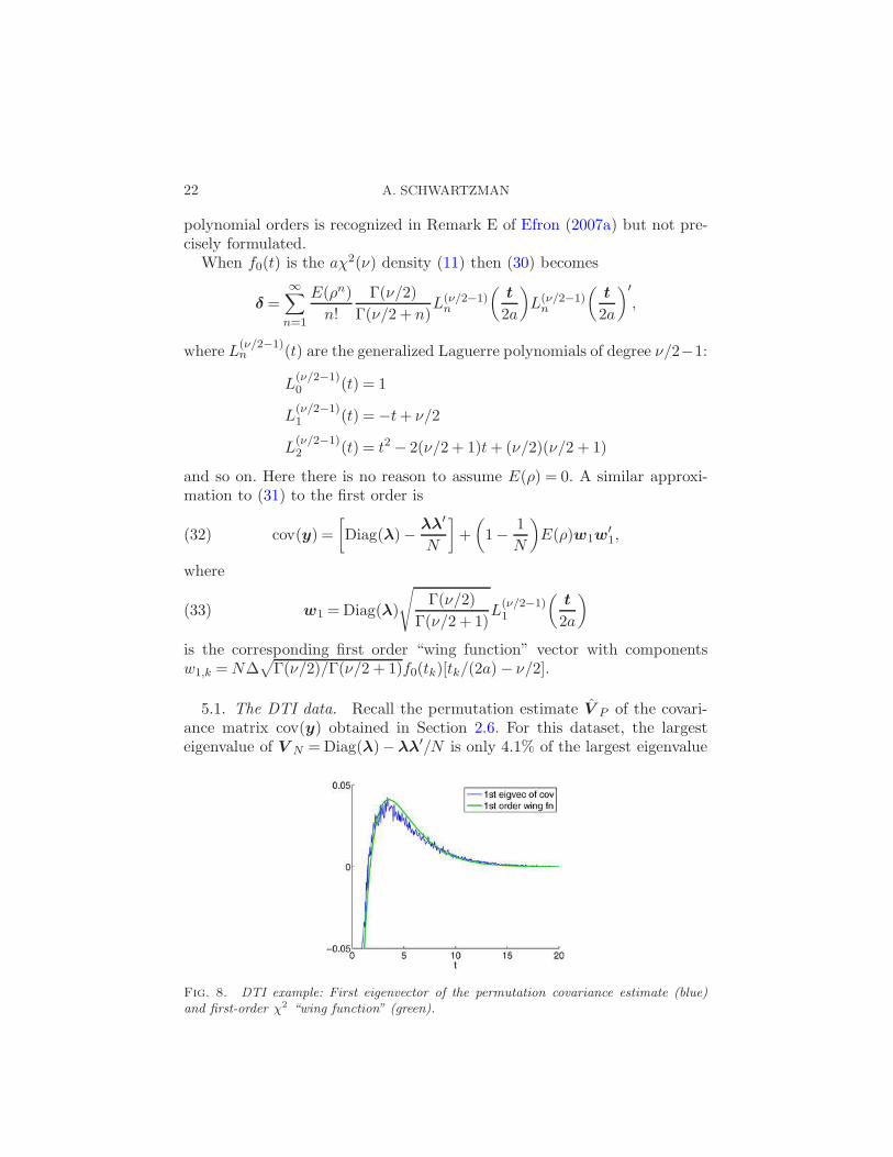
5.1. The DTI data. Recall the permutation estimate V P of the covari-ance matrix cov(y) obtained in Section 2.6. For this dataset, the largesteigenvalue of V N =Diag(λ)−λλ′/N is only 4.1% of the largest eigenvalue

Fig. 8. DTI example: First eigenvector of the permutation covariance estimate (blue)and first-order χ2 “wing function” (green).

EMPIRICAL NULL FOR EXPONENTIAL FAMILIES 23

d1 of V P , while the second eigenvalue d2 of V P is only 6.6% of d1. Thus,using (32), we can approximate

V P ≈E(ρ)w1w′

1,(34)

where w1 is the first-order “wing function” (33) evaluated using the em-

pirical null estimates λ, ν and a from Section 2.5. Figure 8 shows the firsteigenvector of V P superimposed with w1 normalized to unit norm, that is,w1/‖w1‖ with ‖w1‖2 =

∑Kk=1 w

21,k. The similarity between the two is akin

to the similarity between the 1st eigenvector of the permutation covarianceestimate and the 2nd order wing function in the normal example describedin Efron (2007a).

Given the equivalence (34), one might be tempted to estimate the average

pairwise correlation between the test statistics as E(ρ) = d1‖w1‖2 = 0.0057,

where d1 is the largest eigenvalue of V P . This is a strongly conservativeestimate, as it suffers from the upward sorting bias of d1. The true aver-age pairwise correlation is probably much lower. This is reassuring as thecorrelation is presumably mostly local in the image domain.

6. Summary and discussion. In this article I have extended the centralmatching method for estimating the null density in large-scale multiple test-ing to a mode matching method, applicable when the theoretical null belongsto any exponential family or a related distribution such as t or F . The em-pirical null estimate is accompanied by an estimate of p0, the proportionof true null tests in the data. Further, the empirical null estimates can beused directly to estimate local and tail FDR curves for FDR inference. Deltamethod covariance estimates and bias formulas have been derived. We haveseen that FDR estimates are biased down at the far tails and should betaken cautiously whenever the corresponding observed bin counts are small.The effect of correlation has been explained by a generalization of Efron’s“wing function.”

Efron (2005b, 2007b) discusses several reasons why the empirical null maynot match exactly the theoretical null in observational studies. It should beemphasized that mode matching does not necessarily increase power withrespect to the theoretical null [Efron (2004) provides counterexamples]. In-stead, the empirical null answers a question of model validity.

In the normal case, another empirical null method called MLE fitting[Efron (2007b)] has been reported to give similar empirical null estimateswith slightly lower variance. Mode matching is easier to analyze and is ap-pealing because of its application to exponential families. It is also easierto implement in practice because of available software and computationalefficiency. But, in principle, just like mode matching, MLE fitting could beextended to other distributions beyond the normal too.

24 A. SCHWARTZMAN

At least two aspects of mode matching may benefit from further studybeyond this paper. One aspect is the possibility of choosing data-dependentlimits for the fitting interval S0. Fixed limits based on the theoretical null areinappropriate precisely because the empirical null is expected to be displacedor scaled with respect the theoretical null. For instance, in an analysis ofχ2-scores, Schwartzman, Dougherty and Taylor (2008a) used as upper limitthe 90th percentile of the empirical test statistic distribution. In the SNPdata example above, a bootstrap analysis showed that setting the upperlimit to the 99.95th percentile of the test statistic distribution, rather thanthe 99.95th percentile of the theoretical χ2(4) density (the value 20 usedpreviously), results in empirical null variance estimates that are about 50%higher than those obtained when the limit was fixed. This suggests thatthe cost of a data-dependent limit might not be too high. Unfortunately, asshown in Section 4 above, the choice of the limit depends very much on thealternative distribution and the null proportion, both of which are unknown.

Another aspect is the possibility of using the two-step approach of Efron(2007b) of estimating the mixture density nonparametrically before fittingthe empirical null by mode matching. As noted above, the most crucial issueis the bias in the tails of the density. Future exploration may yield an answerto what is the best way to estimate the mixture density for mode matching.For example, different bin widths ∆ could be used inside and outside thefitting interval S0 since they serve different purposes. Inside S0 one couldoptimize ∆ for empirical null estimation, while outside S0 one could optimize∆ for FDR estimation.

Matlab functions implementing the methods described in this paper areavailable at http://biowww.dfci.harvard.edu/˜armin/software.html.

APPENDIX A: SPECIAL CASES

A.1. Normal family. The empirical null N(µ,σ2) with θ = (µ,σ2) hasexponential family form

x(t) = (t, t2)′, ψ(η) =− η214η2

− 1

2log(−2η2)

η = (η1, η2)′ =

(µ

σ2,− 1

2σ2

)′

, g0(t) =1√2π.

The Poisson regression (8) using t and t2 as predictors and log(N∆/√2π)

as offset gives estimates η1, η2 and C. From these we obtain

µ=− η12η2

, σ2 =− 1

2η2, log p0 = C + ψ(η).

EMPIRICAL NULL FOR EXPONENTIAL FAMILIES 25

The parameter derivative matrix D required for computing the covariance

(15) of θ+ = (log p0, µ, σ2)′ is

D =∂θ+

∂(η+)′=

1 − η12η2

η214η22

− 1

2η2

0 − 1

2η2

η12η22

0 01

2η22

=

1 µ µ2 + σ2

0 σ2 2µσ2

0 0 2σ4

.

The normal family N(µ,σ2) lends itself to two exponential subfamilies.

A.1.1. Estimate θ = µ. The empirical null N(µ,σ20) with fixed σ20 has

the exponential family form x(t) = t, η = µ/σ20 , ψ(η) = σ20η2/2 and g0(t) =

e−t2/(2σ20)/√2πσ20 . Poisson regression using t as predictor and log(N∆g0(t))

as offset gives estimates η and C. From these we obtain

µ= σ20η, log p0 = C +σ20η

2

2, D =

(1 µ0 σ20

).

A.1.2. Estimate θ = σ2. The empirical null N(µ0, σ2) with fixed µ0 has

the exponential family form x(t) = (t−µ0)2, η =−1/(2σ2), ψ(η) = (−1/2)×log(−2η) and g0(t) = 1/

√2π. Poisson regression using (t−µ0)

2 as predictor

and log(N∆/√2π) as offset gives estimates η and C. From these we obtain

σ2 =− 1

2η, log p0 = C − 1

2 log(−2η), D =

(1 σ2

0 2σ4

).

A.2. Scaled χ2 family (Gamma). The empirical null aχ2(ν) (11) with

θ = (a, ν)′ has exponential family form

x(t) = (t, log t)′, ψ(η) = log

(Γ(η2 + 1)

(−η1)η2+1

)

η = (η1, η2)′ =

(− 1

2a,ν

2− 1

)′

, g0(t) = 1.

The Poisson regression (8) using t and log t as predictors gives estimates η1,

η2 and C. From these we obtain

a=− 1

2η1, ν = 2(η2 +1), log p0 = C +ψ(η).

26 A. SCHWARTZMAN

The parameter derivative matrix D required for computing the covariance(15) of θ+ = (log p0, a, ν)

′ is

D =

1 − η2 +1

η1Ψ(η2 +1)− log(−η1)

01

2η210

0 0 2

=

1 aν Ψ(ν/2) + log(2a)0 2a2 00 0 2

,

where Ψ(z) = (d/dz) log Γ(z) is the Digamma function. The scaled χ2 familylends itself to two exponential subfamilies.

A.2.1. Estimate θ = a. The empirical null aχ2(ν0) with fixed ν0 has ex-ponential family form x(t) = t, η = −1/(2a), ψ(η) = −(ν0/2) log(−η) andg0(t) = tν0/2−1/Γ(ν0/2). Poisson regression using t as a predictor and log(N∆g0(t))

as offset gives estimates η and C. From these we obtain

a=− 1

2η, log p0 = C − ν0

2log(−η), D =

(1 aν00 2a2

).

A.2.2. Estimate θ = ν. The empirical null a0χ2(ν) with fixed a0 has

exponential family form x(t) = log t, η = ν/2− 1, ψ(η) = logΓ(η+1) + (η+1) log(2a0) and g0(t) = e−t/(2a0). Poisson regression using log t as a predictor

and log(N∆g0(t)) as offset gives estimates η and C. From these we obtain

ν = 2(η +1), log p0 = C +ψ(η), D =

(1 Ψ(ν/2) + log(2a0)0 2

).

APPENDIX B: PROOFS

Proof of Proposition 1. The score equation for the Poisson regres-sion (8) including the external weights W is

X ′W [y − exp(Xη+ +h)] = 0.(35)

The rate of change of the MLE vector η+ with respect to the count vectory, considered as continuous, is

∂η+

∂y′= (X ′WV X)−1X ′W ,(36)

EMPIRICAL NULL FOR EXPONENTIAL FAMILIES 27

obtained by differentiating (35) with respect to y and replacing (9). Condi-

tional on N , the covariance estimate of y is V N . Thus, the delta methodcovariance estimate of η+ is (∂η+/∂y′)V N (∂η+/∂y′)′, yielding (14).

The rate of change of θ+ with respect to η+ is

D =∂θ+

∂(η+)′=∂(log p0,θ(η)

′)′

∂(C,η′)=

(1 ψ(η)′

0 θ(η)′

),(37)

so the rate of change of θ+ with respect to η+ at η is D =D(η). The delta

method covariance estimate of θ+ is (∂θ+/∂(η+)′) cov(η+)(∂θ+/∂(η+)′)′,yielding (15). �

Proof of Proposition 2. The rate of change (16) of the vector log y =Xη+ with respect to y follows directly by (36). By the chain rule, ∂y/∂y′ =

[∂y/∂(logy)′][∂(logy)/∂y′] = V Dy , and similarly, ∂(y− y)/∂y′ = I−V Dy.The result follows by the delta method. �

Proof of Proposition 3. (a) Follows immediately by the delta methodand the definition of A.

(b) To evaluate the rate of change of the vector log(Sy) with respect toy, compute

∂(log(Sy))k∂yl

=∂

∂yllog

(1

2yk +

K∑

j=k+1

yj

)=

12∂yk∂yl

+∑K

j=k+1∂yj∂yl

12 yk +

∑Kj=k+1 yj

.

Thus,

∂(log(Sy))

∂y′= U

−1S∂y

∂y′= U

−1S · V ∂(log y)

∂y′= U

−1SV Dy,

where we have used the fact that ∂(log yk)/∂yl = (1/yk)∂yk/∂yl. The resultnow follows by the delta method and the definition of B. �

Proof of Proposition 4. Dividing the score equation (35) by γ∆ andapplying the law of large numbers as γ→∞ gives that η+ converges to thesolution η+

∞of the equation

X ′W [p0f0 + (1− p0)fA −Diag(g0(t)) exp(Xη+∞)] = 0.(38)

In particular, if p0 = 1, we have that η+ is asymptotically unbiased, that is,η+∞

= (0,η′)′. The idea is to find a first order expansion of η+ near p0 = 1.Differentiating (38) with respect to p0, we obtain that, at p0 = 1, dη+

∞/dp0 =

(X ′W Diag(f0)X)−1X ′W (f0 − fA). The bias in the estimation of η+ isapproximately

η+∞

− η+ = η+∞

− (0,η′)′ − (log(p0),0′)′

≈ dη+∞

dp0

∣∣∣∣p0=1

(p0 − 1)− (log(p0),0′)′,

28 A. SCHWARTZMAN

yielding (26). Similarly, the bias in the estimation of θ+ is a first orderexpansion of θ+ with respect to η+ near p0 = 1. �

Proof of Proposition 5. (a) For known p0 and f0, (18) says fdrk =λk,0/yk, where yk ∼ Po(λk), λk = γ∆f(tk) and λk,0 = γ∆p0f0(tk). Thus,

E[fdrk|yk > 0] = E

(λk,0yk

∣∣∣yk > 0

)=λk,0λk

E

(λkyk

∣∣∣yk > 0

)= fdrk ·ζ(λk),

where ζ(λ) is defined for a generic y ∼ Po(λ) as ζ(λ) = E(λ/y|y > 0). Bydirect evaluation,

ζ(λ) =1

1− e−λ

∞∑

j=1

λ

j

e−λλj

j!=

λ

eλ − 1

∫ λ

0

∞∑

j=1

uj−1

j!du

=λ

eλ − 1

∫ λ

0

du

u

∞∑

j=1

uj

j!,

which is equal to (27).

(b) When the empirical null is used, the local fdr estimate (18) is fdrk =

yk/yk, where yk =N∆p0f0(tk). Notice that when evaluated at tk /∈ S0, thenumerator yk is independent of the denominator yk. Thus,

E[fdrk|yk > 0] = E

(ykyk

∣∣∣yk > 0

)=λk,0λk

E(yk)

λk,0E

(λkyk

∣∣∣yk > 0

)≈ fdrk bkζ(λk),

where the vector b∞ is obtained as follows. By (8) and (9), λ0 = exp(Xη++h) and E(y) = E[exp(Xη+ + h)] → exp(Xη+

∞+ h) as N → ∞. Dividing

entry by entry gives b∞ = exp(X(η+∞

− η+)). �

Proof of Theorem 1. The form of expression (29) follows from Efron(2007a), Lemma 1. A similar argument as in Efron (2007a), Lemma 2, givesthat the entries of δ are

δkl ≈∫ 1

−1Rkl(ρ)dG(ρ), Rkl(ρ) =

f0(tk, tl;ρ)

f0(tk)f0(tl)− 1.(39)

Replacing (28) in (39) gives (30). �

Acknowledgments. The author thanks Bradley Efron and Jonathan Tay-lor for their guidance, Bob Dougherty for providing the DTI data, andChristoph Lange for providing the FBAT analysis results from the FHSSNP data.

EMPIRICAL NULL FOR EXPONENTIAL FAMILIES 29

REFERENCES

Abramowitz, M. and Stegun, I. A., eds. (1966). Handbook of Mathematical Functions

with Formulas, Graphs, and Mathematical Tables, 9th ed. Dover, New York. MR0208797

Benjamini, Y. and Hochberg, Y. (1995). Controlling the false discovery rate: A practical

and powerful approach to multiple testing. J. Roy. Statist. Soc. Ser. B 57 289–300.

MR1325392

Efron, B. (2004). Large-scale simultaneous hypothesis testing: The choice of a null hy-

pothesis. J. Amer. Statist. Assoc. 99 96–104. MR2054289

Efron, B. (2005b). Bayesians, frequentists and scientists. J. Amer. Statist. Assoc. 100

1–5. MR2166064Efron, B. (2007a). Correlation and large-scale simultaneous hypothesis testing. J. Amer.

Statist. Assoc. 102 93–103. MR2293302

Efron, B. (2007b). Size, power and false discovery rates. Ann. Statist. 35 1351–1377.

MR2351089

Efron, B. (2008). Simultaneous inference: When should hypothesis testing problems be

combined? Ann. Appl. Statist. 2 197–223.

Efron, B. and Tibshirani, R. (1996). Using especially designed exponential families for

density estimation. Ann. Statist. 24 2431–2461. MR1425960

Efron, B., Tibshirani, R., Storey, J. D. and Tusher, V. (2001). Empirical Bayes

analysis of a microarray experiment. J. Amer. Statist. Assoc. 96 1151–1160. MR1946571

Everitt, B. S. and Bullmore, E. T. (1999). Mixture model mapping of brain activation

in functional magnetic resonance images. Human Brain Mapping 7 1–14.

Genovese, C. R. and Wasserman, L. (2004). A stochastic process approach to false

discovery control. Ann. Statist. 32 1035–1061. MR2065197

Ghahremani, D. and Taylor, J. E. (2005). Empirical and theoretical false discovery

rate analyses for fMRI data. Poster, Organization for Human Brain Mapping.

Herbert, A., Gerry, N. P., McQueen, M. B., Heid, I. M., Pfeufer, A., Illig,

T., Wichmann, H.-E., Meitinger, T., Hunter, D., Hu, F. B., Colditz, G., Hin-

ney, A., Hebebrand, J., Koberwitz, K., Zhu, X., Cooper, R., Ardlie, K., Lyon,

H., Hirschhorn, J. N., Laird, N. M., Lenburg, M. E., Lange, C. and Christ-

man, M. F. (2006). A common genetic variant is associated with adult and childhood

obesity. Science 312 279–283.

Jin, J. and Cai, T. T. (2007). Estimating the null and the proportion of nonnull effects

in large-scale multiple comparisons. J. Amer. Statist. Assoc. 102 495–506. MR2325113Kong, S. W., Pu, W. T. and Park, P. J. (2006). A multivariate approach for integrating

genome-wide expression data and biological knowledge. Bioinformatics 22 2373–2380.

Kotz, S., Balakrishnan, N. and Johnson, N. L. (2000). Bivariate and trivariate normal

distributions. In Continuous Multivariate Distributions 1. Models and Applications 251–

348. Wiley, New York. MR1792994

Koudou, A. E. (1998). Lancaster bivariate probability distributions with Poisson, nega-

tive binomial and gamma margins. Test 7 95–110. MR1650839

Lange, C., Silverman, E. K., Xu, X., Weiss, S. T. and Laird, N. M. (2003). A mul-

tivariate family-based association test using generalized estimating equations: FBAT-

GEE. Biostatistics 4 195–206.

Lee, J., Shahram, M., Schwartzman, A. and Pauly, J. M. (2007). A complex data

analysis in high-resolution SSFP fMRI. Magn. Reson. Med. 57 905–917.

Patel, J. K. and Read, C. B. (1996). Handbook of the Normal Distribution, 2nd ed.

Dekker, New York.

30 A. SCHWARTZMAN

Schwartzman, A., Dougherty, R. F., Lee, J., Ghahremani, D. and Taylor, J. E.

(2008b). Empirical null and false discovery rate analysis in neuroimaging. Neuroimage.To appear. Available at http://dx.doi.org/10.1016/j.neuroimage.2008.04.182.

Schwartzman, A., Dougherty, R. F. and Taylor, J. E. (2005). Cross-subject com-parison of principal diffusion direction maps. Magn. Reson. Med. 53 1423–1431.

Schwartzman, A., Dougherty, R. F. and Taylor, J. E. (2008a). False discovery rateanalysis of brain diffusion direction maps. Ann. Appl. Statist. 2 153–175.

Storey, J. D. (2003). The positive false discovery rate: A Bayesian interpretation andthe q-value. Ann. Statist. 31 2013–2035. MR2036398

Storey, J. D., Taylor, J. E. and Siegmund, D. (2004). Strong control, conservativepoint estimation and simultaneous conservative consistency of false discovery rates: Aunified approach. J. R. Stat. Soc. Ser. B Stat. Methodol. 66 187–205. MR2035766

Sun, W. and Cai, T. T. (2007). Oracle and adaptive compound decision rules for falsediscovery rate control. J. Amer. Statist. Assoc. 102 901–912.

Van Steen, K., McQueen, M. B., Herbert, A., Raby, B., Lyon, H., DeMeo, D.

L., Murphy, A., Su, J., Datta, S., Rosenow, C., Christman, M., Silverman,

E. K., Laird, N. M., Weiss, S. T. and Lange, C. (2005). Genomic screening andreplication using the same data set in family-based association testing. Nature Genetics37 683–691.

Department of Biostatistics

Harvard School of Public Health

Dana-Farber Cancer Institute

44 Binney Street, CLS-11007

Boston, Massachusetts 02115

USA

E-mail: armins@hsph.harvard.edu