Harvard Institute of Economic...

HH II EE RRHarvard Institute of Economic Research

Discussion Paper Number 1925

Is There A New Urbanism?The Growth of U.S. Cities in

the 1990sBy

Edward L. Glaeser and Jesse Shapiro

June 2001

Harvard UniversityCambridge, Massachusetts

This paper can be downloaded without charge from the:

http://post.economics.harvard.edu/hier/2001papers/2001list.html

IS THERE A NEW URBANISM?

THE GROWTH OF U.S. CITIES IN THE 1990S

by

Edward L. Glaeser1 Harvard University, Brookings Institution and NBER

and

Jesse Shapiro Harvard University

June 12, 2001

ABSTRACT

The 1990s were an unusually good decade for the largest American cities and, in particular, for the cities of the Midwest. However, fundamentally urban growth in the 1990s looked extremely similar to urban growth during the prior post-war decades. The growth of cities was determined by three large trends: (1) cities with strong human capital bases grew faster than cities without skills, (2) people moved to warmer, drier places, and (3) cities built around the automobile replaced cities that rely on public transportation. In the 1990s (as in the 1980s), more local government spending was associated with slower growth, unless that spending was on highways. We shouldn’t be surprised by the lack of change in patterns of urban growth, after all the correlation of city growth rates across decades is generally over 70 percent.

1 Glaeser thanks the National Science Foundation for financial support.

2

I. Introduction

In the 1950s, 60s, and 70s, almost every Northeastern or Midwestern city with more than

500,000 people shrank in every decade.2 In the 1990s, a majority of such cities grew. New

York City’s population grew by nine percent. Chicago grew by four percent. Between 1950 and

1990, the share of Americans living in cities with more than 500,000 inhabitants fell every

decade from a high of 17.54 percent in 1950 to 12.09 percent in 1990. In the 1990s, the share of

population living in these big cities finally rose. Likewise, the share of the U.S. population living

in cities with more than 7500 people per square mile rose from 7.1 percent to 7.8 percent during

the 1990s.

Does this mean that city living is back? Is the New Urbanism movement (Katz, 1994), which

sees a renewed demand for dense, walking cities, correct? Does the 2000 U.S. Census tell us

that the production and consumption benefits of density have finally acted to reverse the slide of

America’s largest cities? Were the 1990s a radical break from the past, during which the

demand for density has finally ended the push towards sprawl and the sun?

No. The growth rates of New York and Chicago were not representative of other dense cities,

which generally declined. Unless we are comfortable extrapolating from these two places we

cannot say that there was a major change in the basic path of urban America. Moreover, the

increase in the growth rates of New York and Chicago between the 1980s and the 1990s was

only slightly higher than the increase in the growth rate of the total U.S. population. Indeed, the

most striking fact about city growth in the 1990s is the continuity with previous decades. City

growth in the 1990s followed the same basic patterns found by previous researchers (Mills and

Lubuele, 1995; Glaeser et al., 1995): there was no general rebirth of high-density cities. The

century-long trend of people moving to places with good weather, low density and skilled

inhabitants, just continued. With the sole exceptions of New York and Chicago, the only dense

cities with more than 200,000 people that grew were either in California or Florida, or were

unusually endowed with college graduates.3 On average, the 18 dense cities without a

2 The only exceptions are Milwaukee in the 1950s and Columbus in the 1970s. 3 Throughout this paper, we use the same terminology as the census and use the term city to refer to the political unit. Technically, the fact that lies behind this sentence is that the only cities with more than 200,000 people which

3

preponderance of skill that are outside of California or Florida declined by more than 5 percent

in the 1990s.

These facts highlight the three important trends in urban growth that persisted throughout the

20th century. There was a flight to warm, dry places. Places built around the car replaced places

built around walking and public transportation. People moved to cities with strong skill bases.

Despite New York and Chicago, these facts remained strong in the 1990s.

Indeed, dryness and temperature were powerful predictors of growth at the city and the MSA

level with or without region controls. The raw correlation of January temperature with city

growth in the 1990s was 35 percent, and the raw correlation of rainfall with city growth was -41

percent. Rainfall and July temperature even remain significant when we control for region

dummies. The magnitudes of these relationships were the same for the 1980s and the 1990s—

we must conclude that the demand for warm weather continued unabated.

The trend to sprawl also persisted. Low-density cities grew faster than high-density cities.

Cities with public transportation systems on average grew slower than cities where people

generally drive. Naturally, we do not interpret this as an estimate of the causal impact of public

transportation. Instead, to us this correlation indicates the ongoing trend away from cities built

around older transportation technologies. Moreover, the impact of density and transport

variables on growth was unchanged between the 1980s and the 1990s.

The high-density cities that tended to succeed were those with strong human capital bases.

Variables like percent college educated remained persistent predictors of growth, especially

outside of the west. The correlation between percent college graduate and the growth rate for

cities with more than 200,000 people outside of the west was 60 percent (shown in Figure 1).

Per capita income was also a strong predictor of growth. Poverty and unemployment

negatively predicted growth. We interpret this (as we have in the past, see Glaeser et al., 1995)

as evidence for the importance of local human capital in growth. The connection between skills

had density levels above the median for that group which grew in the 1990s were (1) either in the New York or Chicago CMSAs or in the states of California or Florida, or (2) were in the top-quarter of big, dense cities when cities are ranked by the share of their population that has a college degree.

4

and growth emphasized by Glaeser (1994) and shown to exist for every decade since 1880 by

Simon and Nardinelli (1996) persisted in the 1990s. Despite the continuing strength of this fact,

we do not know if local skills matter because of education spillovers in production or quality of

life. Even if skills matter primarily for production, we do not know if they matter because

knowledge leads to new ideas or because knowledge is a level effect that is increasingly valued

in an increasingly idea-oriented economy.

Other relationships also remained similar to findings for earlier periods. Cities with more

government spending did worse than cities with small governments. Manufacturing cities tended

to do poorly (as in Glaeser et al., 1995). Surprisingly, employment in the health care industry

was highly negatively correlated with urban growth. City population remained only very weakly

correlated with city growth. As has been shown elsewhere (Glaeser et al., 1995, Eaton and

Eckstein, 1997) there doesn’t appear to be a strong tendency for urban populations to mean

revert. That fact continued to be true in the 1990s.

The fact that urban trends basically continued in the 1990s doesn’t make the data from the 1990s

any less important. The facts have confirmed that we are witnessing a century-long movement

towards better weather, and away from higher density public transportation and low skill cities.

Furthermore, these facts stress the remarkable persistence of urban growth. As Figure 2 shows,

the correlation between urban growth in the 1980s and urban growth in the 1990s was over 75

percent. This extraordinarily high correlation is something of a puzzle in and of itself.

The New Demand for Density

But what about the heralded growth of big, dense cities? For urban economists, the most salient

fact about the growth of cities in the 1990s is the rebound of big, dense cities. This fact has been

proclaimed. But is it true?

First, cities with more than 200,000 people grew at an average rate of 8.7 percent (8.2 percent if

population weighted). The comparable rate for the U.S. population was 12.3 percent. In the

5

1980s, these larger cities grew by 5.3 percent, but the U.S. population only grew by 9.4 percent

in that decade. If there was a speed-up of the largest cities as a whole, it was small.

But what about the fact that there were some big, dense cities that actually grew and were not in

the Sunbelt? Consider the set of 28 cities that had more than 200,000 people in 1990, that had

density levels in 1990 greater one person per fifth acre (or 2.5 people per half-acre) and that are

not in California or Florida. Within that set of cities there were eleven cities that grew in the

1990s (there were also eleven such cities that grew in the 1980s). A slightly higher percentage

grew in the 1990s, but after all, the U.S. population grew faster too.

Does this growth represent a change from historical patterns? A primary fact about urban

growth is that skills predict growth. In 1990 there were 31 cities with more than 200,000 people

and where college graduates outnumbered high school dropouts. All but one of those cities grew

in the 1990s. The only exception was Washington, D.C. Of the 11 dense, non-sunbelt cities

that grew in the 1990s, eight had more college graduates than high school dropouts (in 1990):

Boston, MA, Omaha, NE, Portland, OR, Honolulu, HI, St. Paul, MN, Minneapolis, MN, Seattle,

WA, and Columbus, OH.

There were only three dense cities with more high school dropouts than college graduates (in

1990) that grew in the 1990s outside of California, Texas and Florida: New York, Chicago and

Jersey City (which is, after all, part of the New York metropolitan area). Thus, we are not really

looking at a widespread phenomenon, we are looking at New York and Chicago.

There are many possible explanations for the success of these cities. They are the densest cities

and therefore this could reflect a demand for super-high density either in production of high idea

commodities or in consumption. These cities could just have done well because of immigrant

population. Indeed, every city in the U.S. with more than 200,000 residents and more than 10

percent of residents foreign born (in 1990) grew in the 1990s, except for Newark (which almost

grew). However, New York and Chicago are really only two data points, and it will be hard to

learn much from them.

6

As much as we might like to believe that there was a general rebound in big, dense cities, it isn’t

really true. The growth rate of bigger cities went up relative to the 1980s, but the change in rates

roughly mirrors the increased growth rate of the U.S. population. Of the eleven dense, non-

sunbelt cities that grew in the 1990s, eight can be explained by the fact that high education cities

generally grow (and they have since 1880, see Simon and Nardinelli, 1996). That leaves three

cities in two metropolitan areas, and while the increased population of New York and Chicago is

impressive, it does not make a trend.

In the next section, we consider a wider range of stylized facts about city growth in the 1990s to

see if there are any major ways in which the 1990s looked different from previous decades.

II. Conceptual Issues and the Estimating Framework

Conceptually, we follow the approach to growth put forward in Glaeser et al. (1995) and further

explicated in Glaeser (2000). We assume that we are always in a spatial equilibrium where (1)

individual utility and (2) the returns to capital are equalized across space. These assumptions are

not critical for the empirical work, but they are helpful in enabling us to write down a

microeconomic system that allows us to interpret the results. Local output for city i at time t

equals βαititit LKA , where itA is city level productivity, itK is city level capital and itL is city level

labor, which we assume equals z times total city population (denoted itN ), where 0 < z � 1. The

z parameter is meant to capture the fact that there are some non-working members of each city.

Capital earns an exogenous rent r (equal to its marginal product assuming perfect competition).

Utility equals ititit PWC / , where itC is a city-level consumption amenity index, itW represents

city-level wages and itP represents city-level prices. This must be equal some utility level u

which is constant across cities. These equations produce the following equality, which must hold

for every city:

(1)

−−

−+

−−+Θ=

it

itittit P

CLogALogNLog

βαα

βα 1

1)(

1

1)( ,

7

where tΘ is a term that is constant across cities.4 Thus, city level population is increasing in

city-level productivity and city-level consumption amenities and declining in city-level prices.

To clarify a few key concepts, we suppose that each city i has a set of K scalar characteristics,

denoted Xi1, …, Xik, … , XiK. We prefer to think of these characteristics as unchanging over time.

Letting Xi be the vector of these characteristics, we assume that ( ) itittiit XALog εδβ ++′= and

that ittiit

it XPC

Log µγ +′=

, where itε and itµ are error terms that are orthogonal in both levels

and changes to any observable characteristics and where ât and ãt are vectors of coefficients

corresponding to the city-level characteristics. The term itδ is orthogonal in levels, but

itititit X ξθδδ +′=−+1 where itξ is a completely orthogonal error term. Using these terms, and

combining the orthogonal error terms, we find that:

(2) itk

kikktktktktit

it XN

NLog ζθγγαββ

βα++−−+−

−−+∆Θ=

∑ +++ )))(1((

1

111

1

where itζ is a completely orthogonal error term. Thus if a characteristic Xk—such as weather—

positively predicts growth, this can come about for three reasons. First, this Xk variable may

have become more important in the production process. This would mean that ktkt ββ >+1 .

Second, this Xk variable may have become more important to consumers either by lowering the

cost of living or raising the general set of local amenities. This would mean that ktkt γγ >+1 .

Finally, this Xk variable may increase the rate of technological growth. This would mean that

0>kθ . We have assumed that there are only dynamic effects in the growth of productivity, but

there may also be city-level attributes that are associated with dynamic changes in the quality of

life.

4 In fact, ( ) ( )( ))()1()(1

1 1 uLogrLogLogzLogt ααβαβα

αα −−−−−

+−=Θ − .

8

We will not attempt to determine why any particular variable is associated with later growth.

However, it is important to note that all of those stories may possibly be true for any predictor of

growth. When wage data for cities in 2000 becomes available, it will be possible (in the spirit of

Glaeser et al., 1995) to determine the extent to which urban attributes are working through

productivity or through amenities.

What characteristics might be thought to be important for urban growth? The literature on

economic growth has long suggested that local spillovers means that local human capital should

be a strong determinant of growth. Size and density might also be important. Casual

observation suggests that the weather might be significant. Finally, industry level and political

variables may also be important determinants of local productivity.

An Aside on the Unit of Analyses—MSAs vs. Cities

Generally the approach of geographic economists tends to focus on Metropolitan Statistical

Areas (MSAs). These are multi-county units that are meant to capture local labor markets.

They are available both in the form of Consolidated Metropolitan Statistical Areas (which are

extremely large) and Primary Metropolitan Statistical Areas (or PMSAs which are somewhat

smaller). We will look at the growth of MSAs, but we will also concentrate on cities.

Cities are, of course, political units that lie within metropolitan areas. They differ wildly in size,

sometimes including the entire MSA, other times consisting only of a small downtown area. As

such, comparing cities with one another does require a certain amount of tolerance for error.

However, there are also good reasons for focusing on cities. They are closer to representing

traditional downtowns. While a firmer geographic construct—such as the population within 10

miles of the central business district—might actually be more attractive, in general data on such

entities are not available. Thus, if we want to know the determinants of growth of downtown

areas—true cities, as distinguished from suburbs, we are generally left to look at cities.

9

Moreover, we may be particularly interested in factors such as human capital spillovers that are

generally thought to operate at a fairly local level. As such, sprawling geographic regions, such

CMSAs, will be far from the appropriate unit of analysis. Because we are interested in the

impact of local amenities, we are attracted to smaller units of observation and hence to cities.

Finally, there are also political questions where cities are the perfect unit of analysis.

III. Data Description—Tables 1 and 2

Our data all comes from the 1980, 1990 and 2000 censuses. We have restricted ourselves to

cities with more than 100,000 inhabitants at of 1990 or 1980 (respectively). Our 1980 and 1990

samples thus contain different cities because of our desire to have uniform selection criteria.

Our previous discussions have tended to focus on cities with more than 200,000 people. This is

useful because these larger cities are more likely to be true central cities, while cities with

between 100,000 and 200,000 people will often be suburbs. Still, to get more statistical

precision, we will be looking at the larger set of cities with more than 100,000 people. For

consistency, our MSA sample will also consist of cities with more than 100,000 people

As discussed in Section II, our approach is to correlate urban growth in the 1990s with city

characteristics in the previous decade. The sources for city (or MSA) level characteristics in

1980 and 1990 include the County and City Data Book, 1988, the County and City Data Book,

1994, and the USA Counties 1998 database. The sources are more precisely detailed in the Data

Appendix.

Tables 1 and 2: Means and Sample Correlations

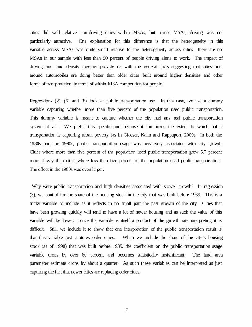
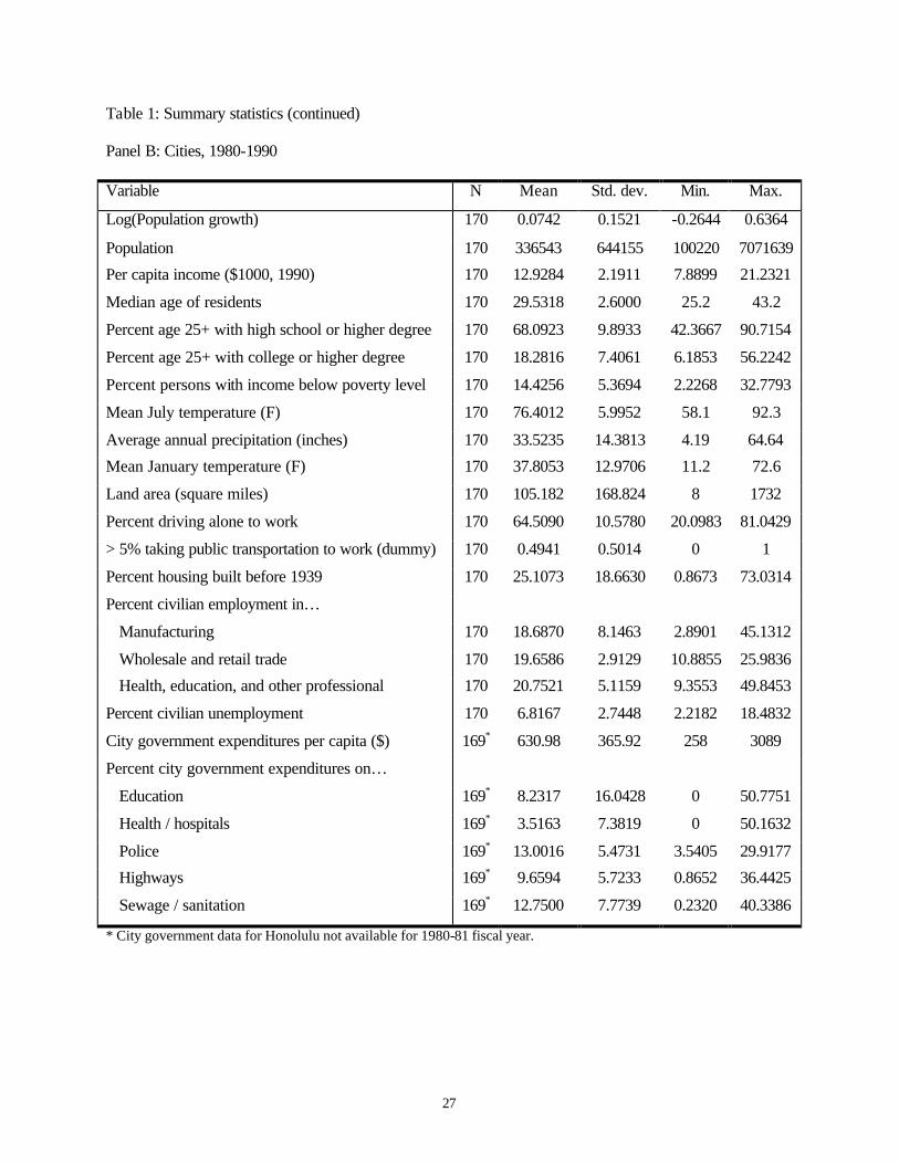
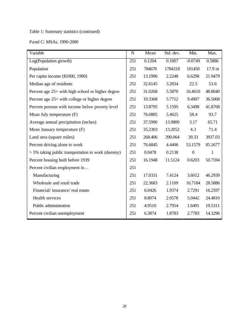
In Tables 1a-1c we show the means and standard deviations of our variables. Among the things

to notice in this data set is that the average log growth rate of cities in the 1990s was 9.76

percent. This is higher than the growth rate in the 1980s, which was 7.42 percent. However, the

difference between the two growth rates was less than the change in overall U.S. population

growth rates between the 1980s and the 1990s. The average growth rate of MSAs was higher,

12.04 percent, which reflects the general rise of the suburbs.

10

The maximum growth rate in both decades was over 60 percent. In the 1980s, the fastest

growing city was Mesa, Arizona. In the 1990s, it was Las Vegas, Nevada. The minimum

growth rate in the 1980s was –26 percent (Gary, Indiana). The minimum growth rate in the

1990s was –13.9 percent (Hartford, Connecticut). The range for MSA growth was comparable

to the range for city growth –7.5 percent to 58.9 percent.

The range in per capita income across cities and MSAs in 1990 was quite vast. The seven

poorest cities were either immigrant cities of the Sunbelt (Laredo, TX, Hialeah, FL, El Monte,

CA) or declining cities of the Rustbelt (Gary, IN, Cleveland, OH, Detroit, MI, Newark, NJ).

The three richest cities were suburbs (Stamford, CT, Alexandria, VA, Irvine, CA). The best

educated cities were college towns (Ann Arbor, MI, Berkeley, CA). The least educated cities

overlapped closely with the poorest cities. By and large the other income and education

variables tend to be highly correlated with one another.

There was also a tremendous amount of heterogeneity in the weather variables. Mean January

temperature as of 1990 ranged from 11.8 degrees (Minneapolis-St. Paul) to 71.4 degrees

(Honolulu, HI). Mean July temperature ranged from the high 50s (Anchorage and San

Francisco) to the low 90s (Phoenix and Las Vegas). Average annual precipitation ranged from

4.13 inches (Las Vegas) to over 65 inches (Tallahassee).

While we group all cities together, some cities are really traditional downtowns and others cover

a wide range of suburbs. The varieties of cities in the data set show up in our sprawl variables.

Some of the smaller cities (which tend to be suburbs) span less than 10 square miles. Among the

larger cities (with more than 500,000 people in 1990), the two smallest cities are Boston and San

Francisco (both are less than 50 square miles). Anchorage is by far the largest city in the U.S.

with more than 1600 square miles. Houston and Oklahoma City are also two of the largest cities.

Public transportation usage tended to be clumped around zero in 1990. In 120 of the 195 cities,

less than four percent of the population used public transportation to get to work. There were 20

cities where more than fifteen percent of the population used public transportation, and in four of

11

these cities more than one-third of the people used public transportation (Washington, D.C.,

Jersey City, NJ, San Francisco, CA, and New York, NY).

Finally, the government variables also show that cities differed a lot in their spending habits. Of

course, much of this heterogeneity comes from state rules about spending—the r-squared from

regressing spending on state dummies is over 70 percent. As such, we will only look at within

state variation when connecting these variables with growth.

In Table 2, we look at correlations between our three measures of city growth and various

dependent variables. We have put stars next to correlations that are statistically significant. The

first line shows the correlation with initial population. In general, there was a slight negative

relationship with initial population for cities and a slight positive relationship for metropolitan

areas. However, in both cases the relationship is statistically insignificant.

However, the relationship with income tended to be quite strong, especially for cities. The

relationships with temperature are particularly striking. Warmth, particularly January

temperature, was highly correlated with growth at both the city and the metropolitan area level.

The sprawl measures—density, car usage and public transportation usage—were all reliably

correlated with growth at the city level. The relationships at the MSA level were much

weaker—perhaps because car usage is almost ubiquitous at the MSA level. The industry mix

variables were occasionally highly correlated with city growth. We are particularly puzzled by

the strong relationship between employment in health services and urban decline at both the city

and MSA levels.

Unemployment was strongly negatively associated with city decline, but much less strongly

associated with MSA decline. As MSAs, not cities, are generally thought to be relevant labor

markets, we interpret this result as suggesting that the city-level correlation is reflecting the

decline of low human capital cities. High school and college degrees both predicted later

growth. Poverty was a strong negative correlate of growth. High percent black was also

12

associated with population decline. This result can either reflect white racism or the correlation

between percent black and poverty, which was over 60 percent in 1990.

Finally, cities with big governments grew much less quickly than cities with small governments.

There was a negative correlation between growth and spending on schooling and a positive

correlation between growth and spending on police. There was also a positive correlation

between growth and spending on highways. Naturally, these spending patterns are interesting

but do not represent causal impacts of spending. They are much more likely to reflect omitted

variables which were correlated both with growth and with these types of spending.

IV. Results

In Table 3, we show our first set of regression results, which focus on the most basic facts of

urban growth. Regressions (1), (5) and (9) look at the degree to which city populations mean

reverted. These regressions show the basic correlation between initial levels of city population

and later growth. Regressions (1) and (5) show that the connection between initial population

and later city growth was stronger in the 1980s than in the 1990s. The connection between initial

population and later growth was more likely to be negative in the past. Glaeser et al. (1995)

found that this was even more true during earlier post-war decades. As regression (9) shows,

there was a statistically insignificant positive relationship between initial MSA population and

later MSA growth in the 1990s.

Regressions (2), (6) and (10) show the connection between population density and later growth

with a three part spline that allows for a more flexible relationship between initial population and

later growth. Again, there was no correlation for cities in the 1990s between population and later

growth. In the 1980s, the correlations were similarly weak. For metropolitan areas, there

appears to have been more of a positive relationship but again there is little here to go on.

The message of these regressions is that in the 1990s, we again saw essentially parallel growth of

both cities and metropolitan areas. There is nothing intrinsic in big cities that makes them

decline. The spline suggests that there is no threshold that cities need to reach before they take

13

off. Overall, as in Glaeser et al. (1995) and Eaton and Eckstein (1997), the evidence supports the

view that city growth is independent of initial city size. Figure 3 shows the relationship between

city growth and the logarithm of city population. The variance of city growth was

unquestionably higher for cities with lower population levels, but there was no effect of city

population on mean growth.

Regressions (3), (7) and (11) include our basic controls: initial income, median age of city

residents and regions. All three of these types of variables related strongly to growth. Income

was a very powerful predictor of later growth. This appears to have been true in the 1980s as

well (but not in earlier decades, see Glaeser et al., 1995). In the 1980s, the effect was less

statistically significant, but the magnitude was actually larger. As wages are, in part, the visible

evidence of human capital, these results are our first hint that the human capital level of the city

was actually important. Of course, this result could also just represent the possibility that some

cities were hit with positive labor demand shocks that then induced migrants to come to the city.

Regression (3), (7) and (11) also show that cities with more young people tended to grow more

quickly than cities with more old people. This is perhaps because younger people tend to move

more often than the old and growing cities tend to attract a larger number of young people.

Finally, we control for region. Regional effects on city growth were quite impressive. The

impact of being in the west was a 15 percent increase in growth (relative to being in the

northeast). Cities in the south grew more than 10 percent faster than cities in the northeast.

These effects were almost the same at the city and the MSA level. The parallel impact of region

on the two geographic units means that the big regional fact is just uneven population growth,

not uneven development of cities.

When we compare the role of regions in the 1980s and 1990s, we see that there were two

changes between the decades. First, in the 1990s, midwestern cities did better than northeastern

cities. In the 1980s, northeastern cities did better. Controlling for other variables, this represents

roughly an 8 percent swing in relative performance. Second, the south did better in the 1990s

(relative to the northeast or the west) than in did in the 1980s. Put together, these facts tend to

suggest that the center of the U.S. gained ground relative to the coasts in the 1990s.

14

Regressions (4), (8) and (12) include the lagged growth rate of the city. One of the more striking

facts about urban growth is the tremendous persistence of growth rates. The correlation between

the growth rate of cities in the 1980s and cities in the 1990s was 77 percent. Figure 2 shows this

impressive relationship graphically. The effects of including lagged growth in the regressions are

impressive. The r-squared of the basic city-level regression doubles when lagged growth is

included. The coefficient on lagged growth is 0.58 which means that if the city grew 1 percent

more quickly in the 1980s, it grew on average 0.58 percent more quickly in the 1990s.

Many variables become insignificant when lagged growth is included in the regression. The

regional patterns become muted. The regression suggests that controlling for lagged growth, the

northeast was the one loser in the 1990s. The impact of age and income disappears. As

controlling for lagged growth eliminates most of the variation across cities, we will not include

lagged growth in any further regressions, because that would make it impossible for us to use

regressions to understand the patterns of growth across cities. Still, while lagged growth doesn’t

help us to explain the city-specific factors that were correlated with later growth, there is no

question that past growth is the best predictor of future growth.

Geographic Determinism Revisited: Urban Growth and the Weather

In Table 4, we look at the role of the weather. While the discipline of geography has tended to

reject geographic determinism for decades, recent research by Jeffrey Sachs and others (see, for

example, Gallup, Sachs, and Mellinger, 1999) tends to find big connections between the weather

and later economic growth. Previous work of ours (Glaeser et al., 2001; see also Glaeser and

Shapiro, 2001) has emphasized the connection between weather and city growth. That paper

argued that the movement of people to warmer, drier cities suggested an increasing importance

of consumer amenities relative to production facilities. In the framework of the model, this

would mean that ktkt γγ >+1 for climate, and that climate is being valued increasingly highly over

time. This increasing value might occur because of rising incomes. Alternatively, the urban

advantages associated with cold, wet places (proximity to rivers, comfort without air-

conditioning in factories over the summer) might have become less important. As declining

15

transportation costs have eroded the advantages of attributes like proximity to natural resources

or rivers, workers have moved to locales that provide consumption advantages.

The connection between growth and the weather appears to have continued to hold in the 1990s,

but there were some notable differences with prior decades. In the first regression, we look at

the effect of mean July temperature. This variable was an important predictor of growth at both

the MSA and the city level in both the 1980s and the 1990s. A one standard deviation increase

in this variable (6.3 degrees) led to 5.1 percent increase in the growth rate (40 percent of a

standard deviation) in the 1990s. The correct view is that this weather variable was important,

but hardly overwhelming. The connection between temperature and later growth was strong, but

there was sufficient variation that it would be wrong to think that we live in a world where

weather determines urban growth.

In regressions (2), (5) and (8) we look at rainfall. Rainfall was associated with slower growth

both in the 1980s and the 1990s. The impact of rainfall on growth in the 1990s appears to have

been somewhat weaker than in the 1980s, but still the variable remained strong. A one standard

deviation decrease in this variable (15 inches) led to a 4 percent increase in the growth rate over

the decade. People moved to drier climates and this was true at both the city and the MSA level.

In regressions (3), (6) and (9) we look at the impact of January temperature. Among cities in the

1990s, there was no impact of January temperature on growth, once we control for region.

Without regional controls, the effect of January temperature was quite significant—the

correlation between growth and January temperature across the U.S. as a whole was 35 percent.

The decline of January temperature represents a change from the 1980s where January

temperature had a significant effect on city growth. In the 1990s, January temperature still

mattered for MSA growth. The smaller effect of January temperature on cities in the 1990s

seems to represent smaller growth of central cities in some Sunbelt states, mostly California.

While California cities still grew 6 percent faster than our entire sample of cities, they grew 8

percent more slowly than cities in the west more broadly. Since California cities have extremely

16

mild winters (13 degrees warmer than the west generally and 8 percent warmer than our southern

cities), the slow growth of California lessens the impact of this weather variable. 5

Overall, climate was still clearly important. Dry, hot places grew faster probably because they

appeal to consumers. However, the dominance of weather appears to have declined somewhat.

In the 1980s, only four very cold cities (defined as having mean January temperatures below 30

degrees) grew by more than 12 percent. In the 1990s, twelve such cold cities grew that fast. Of

course, in general the cold regions did not do well, but some cold cities have done better.

Understanding this change appears to be an important avenue for future research.

The Rise of Edge Cities

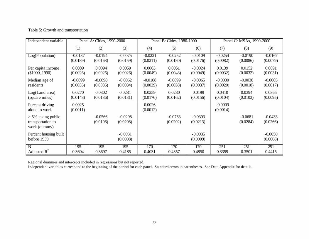
In Table 5, we look at a second phenomenon: the rise of edge cities (Garreau, 1991). The broad

urban history of the 20th century has seen the replacement of higher density cities, built around

public transportation, with medium density cities built around automobiles (see Glaeser and

Kahn, 2001). Table 5 looks at whether this change continued in the 1990s.

Regressions (1), (4) and (7) examine urban density and car use. We include the logarithm of

land area in these cities. Since we are controlling for the logarithm of population, including this

control is equivalent to controlling for density. At the city level, land area had a weakly positive

effect in both the 1980s and 1990s. A one standard deviation increase in land area was related to

a 2 percent increase in the growth rate of cities in both decades. At the MSA level, the impact of

density was much stronger. Big MSAs grew much more quickly than small MSAs.

The proportion of workers driving alone to work also had a correlation with growth at the city

level (but not at the MSA level). As the share of workers who drive rose by 10 percent, the

growth rate over the 1990s rose by 2.5 percent (20 percent of a standard deviation). The impact

of driving in the 80s was almost identical. Interestingly, the coefficient on percent driving is

only statistically significant in the city regressions—not the MSA regressions. Thus, driving

5 Indeed, when we remove cities in California from regression (3) we find a significant positive relationship between January temperature and city growth similar in magnitude to that found in the 1980s.

17

cities did well relative non-driving cities within MSAs, but across MSAs, driving was not

particularly attractive. One explanation for this difference is that the heterogeneity in this

variable across MSAs was quite small relative to the heterogeneity across cities—there are no

MSAs in our sample with less than 50 percent of people driving alone to work. The impact of

driving and land density together provide us with the general facts suggesting that cities built

around automobiles are doing better than older cities built around higher densities and other

forms of transportation, in terms of within-MSA competition for people.

Regressions (2), (5) and (8) look at public transportation use. In this case, we use a dummy

variable capturing whether more than five percent of the population used public transportation.

This dummy variable is meant to capture whether the city had any real public transportation

system at all. We prefer this specification because it minimizes the extent to which public

transportation is capturing urban poverty (as in Glaeser, Kahn and Rappaport, 2000). In both the

1980s and the 1990s, public transportation usage was negatively associated with city growth.

Cities where more than five percent of the population used public transportation grew 5.7 percent

more slowly than cities where less than five percent of the population used public transportation.

The effect in the 1980s was even larger.

Why were public transportation and high densities associated with slower growth? In regression

(3), we control for the share of the housing stock in the city that was built before 1939. This is a

tricky variable to include as it reflects in no small part the past growth of the city. Cities that

have been growing quickly will tend to have a lot of newer housing and as such the value of this

variable will be lower. Since the variable is itself a product of the growth rate interpreting it is

difficult. Still, we include it to show that one interpretation of the public transportation result is

that this variable just captures older cities. When we include the share of the city’s housing

stock (as of 1990) that was built before 1939, the coefficient on the public transportation usage

variable drops by over 60 percent and becomes statistically insignificant. The land area

parameter estimate drops by about a quarter. As such these variables can be interpreted as just

capturing the fact that newer cities are replacing older cities.

18

This fact makes it particularly important to stress that we are not suggesting that our results can

be interpreted as an estimate of the impact of building more public transportation. Cities with

more public transportation grew more slowly in the 1980s and the 1990s, but this was probably

due to a host of factors associated with these relatively old, relatively high-density cities. Indeed,

the effect of public transportation disappears when you control for the age of the housing stock.

People appear to have left public transportation cities, but they did not necessarily do so because

of public transportation itself. Omitted correlates of public transportation are likely to have

caused the shift.

Growth, Industry Structure and Unemployment

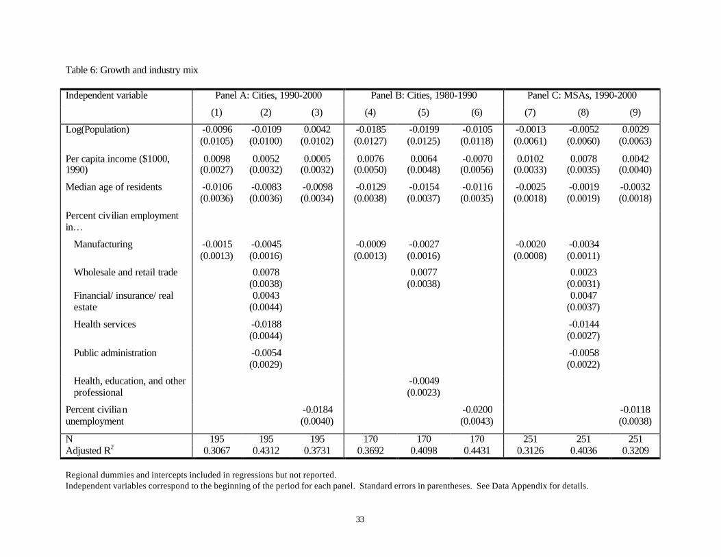
In Table 6, we look at the correlations between growth and initial industrial structure. Past work

(Glaeser et al., 1995) found a connection between manufacturing employment and growth during

earlier post-war decades (particularly the 1950s and 1960s). In the 1980s and 1990s, the effect

of manufacturing employment was negative but statistically insignificant at the city level (as

shown in regressions (1) and (4)). In regression (7), we show that manufacturing still predicted

decline at the MSA level.

In regressions (2), (5) and (8), we include a wider range of industry level controls. Here

manufacturing employment is being compared with professional employment, not with all other

industries. In this case, manufacturing was a significant negative predictor at both the MSA and

the city level. Wholesale and retail trade was significantly positive at the city level but not the

MSA level. We have more limited industrial data in the 1980s, but this data also suggests that

trade employment positively predicted growth at the city level. While the difference between

MSA and city level results makes interpretation difficult, we tend to see this positive impact as

suggesting that commercial cities did well in the 1980s and the 1990s.

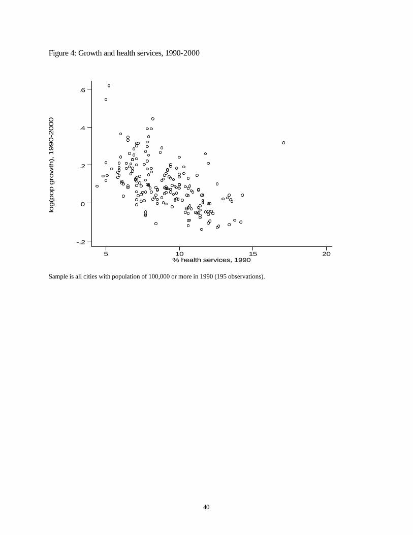
Regressions (2) and (8) do show two industries which appear to have been strongly correlated

with urban decline. Employment in health services turns out to have strongly predicted urban

decline. The remarkable strength of this correlation is shown in Figure 4. We are unsure why

this correlation is so robust, but it is clearly a strong, stylized fact of growth in the 1990s. It is

19

also clear that employment in public administration negatively predicted growth. One

explanation for these industry effects is that these are the industries that remain in declining

cities.

Regressions (3), (6), and (9) look at the impact of urban unemployment. Unsurprisingly, there

was a strong tendency for population to flee high unemployment cities. The magnitude of this

effect was quite large. A one-standard deviation increase in unemployment (2.6 percent) was

related to a 4.8 decrease in the growth rate. As discussed in previous research, this finding can

be interpreted as meaning that population leaves cities with negative labor demand shocks. An

alternative interpretation is that unemployment correlated with low human capital and it was that

lack of human capital that eliminated growth.

Growth and Human Capital

In Table 7, we look at the correlation between city growth and education levels within the cities.

Because of the high correlation between skill levels and average wages (over 70 percent), we

have excluded initial income from these regressions. There are many reasons why education

may be related to city growth. Glaeser (1994) suggested that the relationship might be because

high human capital people produce more new ideas (in the language of the model 0>kθ ).

Alternatively, skilled people might generate static production spillovers and these might have

gotten more important in an increasingly idea-oriented economy (in the language of the model

ktkt ββ >+1 for skilled workers). Finally, skilled people might have become more important for

purely consumption related reasons. Nonetheless, the connection between initial years of

schooling and urban population growth is one of the most remarked upon facts of urban

development (Glaeser, 1994, Glaeser et al. 1995, Black and Henderson, 1999, Simon and

Nardinelli, 1996).

In regressions (1) through (3), we find that there was still a connection between human capital

and later city growth in the 1990s. Figure 1 shows the relationship between percent college-

educated and later growth. We have excluded per capita income because of the high correlation

of this variable with years of schooling. Well educated cities grew by much more than poorly

20

educated cities. As the share of the people in the city aged 25 or more with college degrees rose

by 10 percent in 1990, the expected growth rate of the city in the 1990s rose by 2.3 percent. The

impact of high school degrees on city growth was even stronger. As the share of the population

that are high school dropouts fell by 10 percent, the expected growth rate of the city rose by 3.9

percent. When we include both of these variables, high school appears to have been much more

important than college. Oddly, the impact of education on MSA growth looks quite different, as

shown in regressions (7) through (9). College education was positively associated with MSA

growth, and high school education was actually negatively associated with that growth.

The impact of percent high school graduates in the 1980s and the 1990s was quite similar.

However, percent college educated did not predict urban growth in the 1980s. After looking at

the data in detail, we found that this lack of correlation was completely due to the impact of

California. In California, higher human capital cities tended to grow slowly and low human

capital cities tended to grow quickly. One explanation for this phenomenon is that lower human

capital cities attracted the large inflow of immigrants and the higher human capital cities

imposed growth controls. Whatever the reason, California looked different from the rest of the

U.S. and from historical experience. In that state, human capital deterred growth. Elsewhere, it

encouraged growth. Once we exclude California, the coefficient on percent college graduates is

large and similar across decades and between MSAs and cities. The general tendency of higher

skilled cities to grow quickly seems to be one of the most persistent facts in city growth.

Growth, Race and Poverty

21

In Table 8, we look at the relationship between local poverty and population growth. In both the

1980s and the 1990s, there was a massive negative impact of local poverty. Controlling for this

variable completely eliminates the impact of per capita income (indeed, the effect of this variable

becomes negative in the 1980s). Local poverty was the human capital variable with the strongest

correlation with urban growth. The effect of this variable was indeed massive—as shown in

Figure 5. A one standard deviation increase in the local poverty rate (6.6 percent) caused a 6

percent decrease in the urban growth rate in the 1990s. In the 1980s, the effect was even larger.

The same increase in the poverty rates was related to a growth decline of almost 12 percent.

At the MSA level, there was no effect of local poverty and the effect of per capita income

remained strong. It seems that the bottom end of the human capital distribution was more

important at the city level, but that the mean of the distribution was more important at the MSA

level. The weak effect of poverty at the MSA level corresponds with the negative effect of high

school graduation rates at the MSA level in Table 7. One possible explanation for this fact might

be that poverty at high densities drove down the attractiveness of cities. This mattered less at the

lower densities of MSAs. At the MSA level, human capital might have mattered more because it

increased the rate of growth of new industry.

One question is whether high poverty just reflects low labor demand. To address this possibility,

we look at race. Race is sadly highly correlated with poverty, but it will not be a direct

consequence of lower labor demand (i.e. a city won’t see an mechanical increase in percent black

just because its labor demand falls). Growth decreased strongly with percent black at both the

MSA and the city level. While this effect might reflect white racism, our preferred interpretation

is that this result shows more about the connection between local poverty and urban decline. In

regressions (3), (6) and (9), we look at both variables. At the city level, poverty was more

important than race. At the MSA level, race was more important.

Tables 7 and 8 have together illustrated the continuing importance of human capital in

determining city growth. Skilled cities grew. Unskilled cities declined. To us, this suggests that

urban policy must address local skill levels.

22

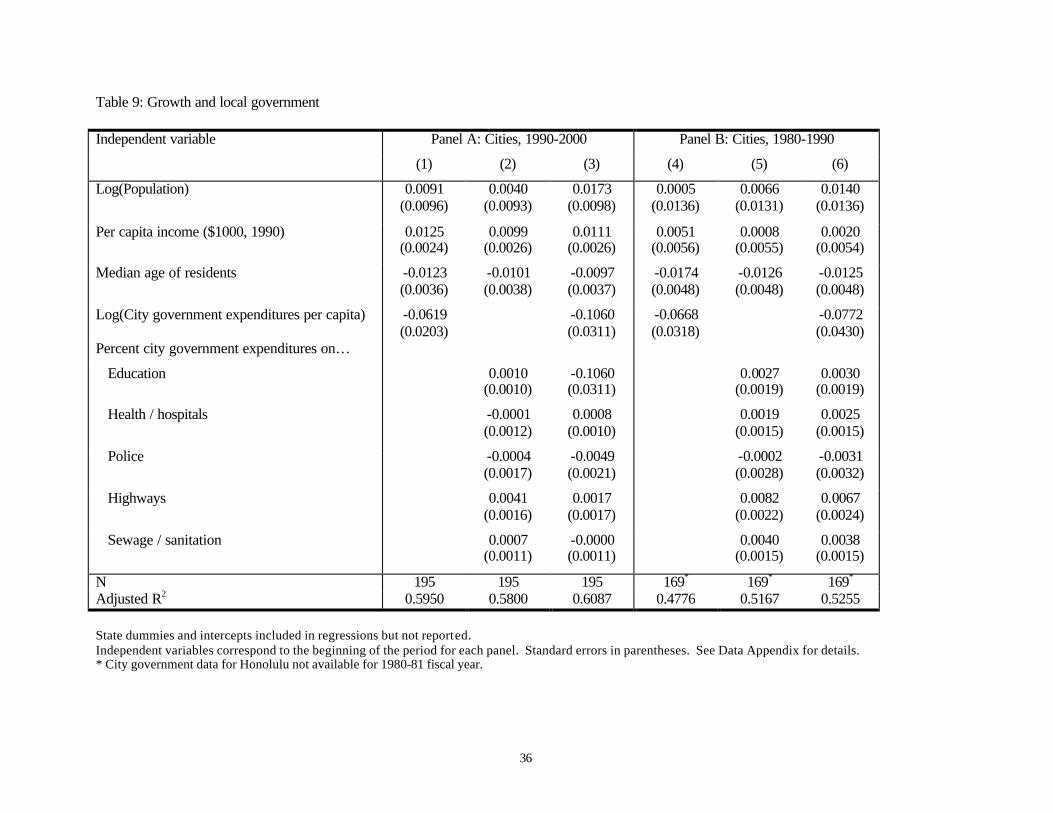
Growth and Government

In Table 9, we look at the correlations between government policy variables and later growth. In

these regressions, we restrict ourselves to cities. MSAs are not governmental units and as such it

makes sense to focus on cities. A problem with this analysis is that in some areas other

governmental units take on city functions. Some types of spending might therefore have been

low in some cities, not because there was little spending on this type of commodity, but because

the commodity was being provided by a different level of government. To correct for this

possibility, we have included state dummies in these regressions.

Regression (1) shows the negative effect of overall city spending on growth in the 1990s. This

effect was fairly large—a one standard deviation increase in government spending was related to

a 3 percent decrease in the growth rate over the decade. In the 1980s, there was also a significant

relationship. Rappaport (1999) also found such a correlation in the 1970s. Earlier Glaeser et al.

(1995) looked at the effect of 1960 government spending on growth over the next 30 years and

found no significant correlation. Thus, it seems that in the middle of the century, big local

governments were not associated with urban decline, but since 1970s, big per capita city

spending negatively predicted local growth.

In regressions (2) and (4), we look at whether there was a relationship between city growth and

the way government spending was allocated. The omitted categories are spending on public

welfare, fire protection, and miscellany in the 1990s and spending on miscellany in the 1980s. In

the 1990s, the only category of spending which was positively correlated with later growth was

highways. This category was positively correlated with growth in the 1980s as well.

Furthermore, the impact of this variable survives controlling for the overall size of government.

We believe that this again supports the importance of the move to sprawled cities.

Other types of government spending—such as schooling—were important correlates of growth

in the past (see Rappaport, 1999) but don’t seem to be correlated with growth in the 1990s.

Police spending was also an important correlate of growth in the 1980s, but not in the 1990s. It

is always hard to interpret the correlation between government spending types and later growth,

23

since spending is likely to be a response to underlying urban conditions. Still, it is important to

know the basic stylized fact of government spending and city growth in the 1990s: cities with

more spending grew less unless that spending was on highways.

V. Conclusion

In this paper, we have examined the correlates of urban growth in the 1990s. In many ways,

growth in the 1990s looked like growth during previous decades. The correlation of growth rates

between the 1980s and the 1990s was extraordinarily high, over 75 percent, and this permanence

makes it unsurprising the basic stylized facts remain. There are three reliable facts about city

growth in the post-war period. People moved to drier, warmer cities. Cities with high levels of

human capital did well and cities with large numbers of the poor did poorly. Lower density

cities that center around cars did better than higher density, public transportation cities. These

facts were true at both the city and MSA level. The 1990s merely confirmed results from

previous decades.

Indeed, this study finds only two modest changes between the 1980s and the 1990s. First, bigger

cities of the Northeast and the Midwest did slightly better in the 1990s than in previous decades.

The post-war era has seen massive decline in those cities. In the 1990s, overall city growth sped

up and those cities declined less often. Second, in the 1990s, Midwestern cities did much better

than they had previously. For example, in the 1980s, no Midwestern city grew by more than 12

percent. In the 1990s, six Midwestern cities grew that quickly.

We therefore think that the fundamental lesson of urban growth in the 1990s is the remarkable

continuity of urban growth patterns. In the last decade, as in all previous post-war decades,

urban growth was driven by the increasing importance of consumers and their tastes for cars,

good weather, and the skill base of the local community.

24

References

Black, Duncan; Henderson, Vernon. (1999) A theory of urban growth. Journal of Political Economy 107(2): 252-284.

Eaton, Jonathan; Eckstein, Zvi. (1997) Cities and growth: Theory and evidence from France and Japan. Regional Science and Urban Economics 27(4-5): 443-474.

Garreau, Joel. (1991) Edge City: Life on the New Frontier. New York: Doubleday.

Gallup, John L.; Sachs, Jeffrey D.; Mellinger, Andrew D. (1999) Geography and economic development. International Regional Science Review 22(2): 179-232.

Glaeser, Edward L. (1994) Cities, information, and economic growth. Cityscape: A Journal of Policy Development and Research 1(1): 9-47.

Glaeser, Edward L.; Scheinkman, Jose A.; Shleifer, Andrei. (1995) Economic growth in a cross-section of cities. Journal of Monetary Economics 36(1): 117-143.

Glaeser, Edward L. (2000) The new economics of urban and regional growth, in The Oxford Handbook of Economic Geography, eds. Gordon L. Clark, Maryann P. Feldman, and Meric S. Gertler. Oxford: Oxford University Press.

Glaeser, Edward L.; Kahn, Matthew E.; Rappaport, Jordan M. (2000) Why do the poor live in cities? NBER Working Paper No. 7636.

Glaeser, Edward L.; Kolko, Jed; Saiz, Albert. (2001) Consumer city. Journal of Economic Geography 1(1): 27-50.

Glaeser, Edward L.; Kahn, Matthew E. (2001) Decentralized employment and the transformation of the American city. NBER Working Paper No. 8117.

Glaeser, Edward L.; Shapiro, Jesse M. (2001) City growth and the 2000 Census: Which cities grew, and why? The Brookings Institution Survey Series.

Katz, Peter (ed.). (1994) The New Urbanism: Toward an Architecture of Community. New York: McGraw-Hill.

Mills, Edwin S.; Lubuele, Luan’ Sende. (1995) Projecting growth of metropolitan areas. Journal of Urban Economics 37(3): 344-360.

Rappaport, Jordan M. (1999) Local economic growth. Harvard University Dissertation.

Simon, Curtis J.; Nardinelli, Clark. (1996) The talk of the town: Human capital, information, and the growth of English cities, 1861 to 1961. Explorations in Economic History 33(3): 384-413.

25

U.S. Dept. of Commerce, Bureau of the Census. (1988) County and City Data Book 1983. Washington: U.S. Department of Commerce, Bureau of the Census, producer. Ann Arbor: Inter-university Consortium for Political and Social Research, distributor.

U.S. Department of Commerce, Bureau of the Census. (1994) County and City Data Book 1994. Washington: U.S. Department of Commerce, Bureau of the Census, Data User Services Division.

U.S. Department of Commerce, Bureau of the Census. (1998) USA Counties 1998. Washington: U.S. Department of Commerce, Bureau of the Census.

26

Table 1: Summary statistics Panel A: Cities, 1990-2000 Variable N Mean Std. dev. Min. Max.

Log(Population growth) 195 0.0976 0.1263 -0.1392 0.6164

Population 195 326813 628524 100217 7322564

Per capita income ($1000, 1990) 195 14.2507 3.3550 6.981 27.092

Median age of residents 195 31.5651 2.3347 25.6 40.1

Percent age 25+ with high school or higher degree 195 75.6754 9.4810 44.3 95.1

Percent age 25+ with college or higher degree 195 22.5103 9.0653 6 64.2

Percent persons with income below poverty level 195 15.7154 6.5878 2.6 37.3

Mean July temperature (F) 195 76.3256 6.3165 58.4 93.5

Average annual precipitation (inches) 195 32.3395 15.1642 4.13 65.71

Mean January temperature (F) 195 39.3405 13.3658 11.8 71.4

Land area (square miles) 195 103.662 159.042 8.4 1697.6

Percent driving alone to work 195 71.9431 10.4294 24 90.1

> 5% taking public transportation to work (dummy) 195 0.3128 0.4648 0 1

Percent housing built before 1939 195 18.2887 16.9102 0 68.1

Percent civilian employment in…

Manufacturing 195 15.7641 6.4885 3.6 40.2

Wholesale and retail trade 195 28.6815 2.4921 11.9 28.7

Financial/ insurance/ real estate 195 7.5015 2.0975 4 15.4

Health services 195 9.0138 2.2660 4.4 17.1

Public administration 195 5.3477 3.3112 1.6 22.2

Percent civilian unemployment 195 7.2010 2.6239 2.8 19.7

City government expenditures per capita ($) 195 1139.50 806.20 347 7154

Percent city government expenditures on…

Education 195 6.7985 15.7716 0 58.7

Health / hospitals 195 2.9303 6.2300 0 59.5

Police 195 14.5072 5.8414 4 31.7

Highways 195 9.4554 5.7375 0.7 38.5

Sewage / sanitation 195 11.8985 7.5386 0 38.2

27

Table 1: Summary statistics (continued) Panel B: Cities, 1980-1990 Variable N Mean Std. dev. Min. Max.


Population 170 336543 644155 100220 7071639




Percent age 25+ with college or higher degree 170 18.2816 7.4061 6.1853 56.2242





Land area (square miles) 170 105.182 168.824 8 1732

Percent driving alone to work 170 64.5090 10.5780 20.0983 81.0429


Percent housing built before 1939 170 25.1073 18.6630 0.8673 73.0314


Manufacturing 170 18.6870 8.1463 2.8901 45.1312


Health, education, and other professional 170 20.7521 5.1159 9.3553 49.8453


City government expenditures per capita ($) 169* 630.98 365.92 258 3089


Education 169* 8.2317 16.0428 0 50.7751

Health / hospitals 169* 3.5163 7.3819 0 50.1632

Police 169* 13.0016 5.4731 3.5405 29.9177

Highways 169* 9.6594 5.7233 0.8652 36.4425

Sewage / sanitation 169* 12.7500 7.7739 0.2320 40.3386

* City government data for Honolulu not available for 1980-81 fiscal year.

28

Table 1: Summary statistics (continued) Panel C: MSAs, 1990-2000 Variable N Mean Std. dev. Min. Max.


Population 251 784670 1784318 101450 17.9 m




Percent age 25+ with college or higher degree 251 19.3368 5.7712 9.4907 36.5068





Land area (square miles) 251 268.406 390.064 39.33 3937.03

Percent driving alone to work 251 76.6845 4.4406 53.1579 85.1677


Percent housing built before 1939 251 16.1948 11.5124 0.6203 50.7594

Percent civilian employment in… 251

Manufacturing 251 17.0331 7.4124 3.6012 46.2939


Financial/ insurance/ real estate 251 6.0426 1.9374 2.7291 16.2597

Health services 251 8.8074 2.0578 5.0442 24.4810

Public administration 251 4.9510 2.7954 1.6491 19.5311


29

Table 2: Simple correlations with log(population growth) Beginning-of-period variable Panel A: Cities,

1990-2000 Panel B: Cities,

1980-1990 Panel C:

MSAs, 1990-2000

Log(Population) -0.0888 -0.1370 0.0988

Per capita income ($1000, 1990) 0.3087* 0.2596* 0.1128

Median age of residents -0.1127 -0.2032* -0.1018

Mean July temperature (F) 0.2436* 0.2125* 0.3795*

Average annual precipitation (inches) -0.4164* -0.4689* -0.1943*

Mean January temperature (F) 0.3506* 0.3988* 0.4146*

Log(Population per square mile) -0.3049* -0.2902* -0.2071*

Percent driving alone to work 0.3119* 0.3015* -0.1406*

> 5% taking public transportation to work (dummy) -0.3566* -0.3609* -0.0883

Percent housing built before 1939 -0.5904* -0.5603* -0.6051*


Manufacturing -0.1487* -0.2441* -0.3524*

Wholesale and retail trade 0.2319* 0.3090* 0.1038

Financial/ insurance/ real estate 0.1967* N/A 0.1860*

Health services -0.5237* N/A -0.3618*

Public administration -0.1070 N/A 0.0802

Health, education, and other professional N/A -0.1392 N/A

Percent civilian unemployment -0.4569* -0.4194* -0.1003

Percent age 25+ with high school or higher degree 0.3750* 0.4500* -0.4916*

Percent age 25+ with college or higher degree 0.2455* 0.2343* 0.2411*

Percent persons with income below poverty level -0.4730* -0.4292* 0.1156

Percent black -0.4989* -0.4682* -0.0684

Log(City government expenditures per capita) -0.3515* -0.3033* N/A


Education -0.2577* -0.1392 N/A

Health / hospitals -0.0983 -0.0944 N/A

Police 0.2122* 0.3098* N/A

Highways 0.3872* 0.3101* N/A

Sewage / sanitation 0.0333 0.0680 N/A

* Correlation statistically significant at the 5% level.

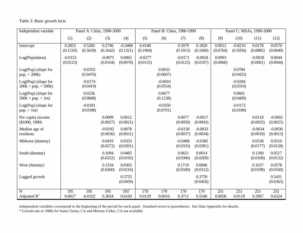
Table 3: Basic growth facts

Panel A: Cities, 1990-2000 Panel B: Cities, 1980-1990 Panel C: MSAs, 1990-2000 Independent variable

(1) (2) (3) (4) (5) (6) (7) (8) (9) (10) (11) (12)

Intercept 0.2853 (0.1518)

0.5260 (0.5639)

0.2746 (0.1642)

-0.3468 (0.1321)

0.4148 (0.1904)

0.5079 (0.1915)

0.1820 (0.1660)

0.0012 (0.0764)

-0.8210 (0.5056)

0.0178 (0.0885)

0.0579 (0.0640)

Log(Population) -0.0153 (0.0123)

-0.0075 (0.0104)

0.0065 (0.0078)

-0.0277 (0.0155)

-0.0171 (0.0125)

-0.0024 (0.0107)

0.0093 (0.0060)

-0.0028 (0.0061)

0.0044 (0.0044)

Log(Pop) (slope for pop. < 200k)

-0.0355 (0.0476)

0.0033 (0.0607)

0.0784 (0.0425)

Log(Pop) (slope for 200k < pop. < 500k)

-0.0174 (0.0419)

-0.0810 (0.0554)

-0.0284 (0.0310)

Log(Pop) (slope for 500k < pop. < 1m)

0.0236 (0.0848)

0.0677 (0.1238)

0.0601 (0.0409)

Log(Pop) (slope for pop. > 1m)

-0.0181 (0.0598)

-0.0350 (0.0791)

-0.0172 (0.0189)

Per capita income ($1000, 1990)

0.0099 (0.0027)

0.0012 (0.0021)

0.0077 (0.0050)

-0.0017 (0.0043)

0.0118 (0.0032)

-0.0002 (0.0025)

Median age of residents

-0.0102 (0.0036)

0.0078 (0.0031)

-0.0130 (0.0037)

-0.0033 (0.0034)

-0.0034 (0.0018)

-0.0030 (0.0013)

Midwest (dummy) 0.0419 (0.0272)

0.0353 (0.0201)

-0.0468 (0.0333)

-0.0385 (0.0281)

0.0538 (0.0177)

0.0510 (0.0128)

South (dummy) 0.1094 (0.0252)

0.0485 (0.0193)

0.0651 (0.0306)

0.0014 (0.0269)

0.1260 (0.0169)

0.0517 (0.0132)

West (dummy) 0.1534 (0.0260)

0.0302 (0.0216)

0.1719 (0.0349)

0.0846 (0.0312)

0.1637 (0.0198)

0.0578 (0.0160)

Lagged growth

0.5755 (0.0459)

0.3759 (0.0456)

0.5431 (0.0363)

N 195 195 195 193* 170 170 170 170 251 251 251 251 Adjusted R2 0.0027 -0.0102 0.3054 0.6169 0.0129 0.0016 0.3711 0.5540 0.0058 0.0119 0.2967 0.6324 Independent variables correspond to the beginning of the period for each panel. Standard errors in parentheses. See Data Appendix for details. * Growth rate in 1980s for Santa Clarita, CA and Moreno Valley, CA not available.

Table 4: Growth and climate


(1) (2) (3) (4) (5) (6) (7) (8) (9)

Intercept -0.2833 (0.1771)

0.2963 (0.1616)

0.2825 (0.1654)

-0.2049 (0.2225)

0.5897 (0.1872)

0.5233 (0.1896)

-0.5252 (0.1145)

0.0471 (0.0883)

0.0400 (0.0877)


-0.0094 (0.0102)

-0.0075 (0.0104)

-0.0207 (0.0116)

-0.0209 (0.0122)

-0.0187 (0.0124)

-0.0119 (0.0058)

-0.0038 (0.0061)

-0.0071 (0.0062)


0.0111 (0.0025)

0.0086 (0.0027)

0.0099 (0.0027)

0.0118 (0.0047)

0.0049 (0.0049)

0.0095 (0.0050)

0.0172 (0.0031)

0.0128 (0.0032)

0.0126 (0.0032)


-0.0097 (0.0033)

-0.0062 (0.0039)

-0.0101 (0.0036)

-0.0127 (0.0035)

-0.0076 (0.0040)

-0.0158 (0.0039)

-0.0034 (0.0017)

-0.0025 (0.0018)

-0.0042 (0.0018)

Mean July temperature (F)

0.0081 (0.0013)

0.0096 (0.0018)

0.0080 (0.0012)

Average annual precipitation (inches)

-0.0026 (0.0009)

-0.0040 (0.0012)

-0.0015 (0.0006)

Mean January temperature (F)

-0.0004 (0.0009)

0.0025 (0.0012)

0.0019 (0.0007)

Midwest (dummy) 0.0303 (0.0251)

0.0191 (0.0281)

0.0402 (0.0275)

-0.0629 (0.0310)

-0.0717 (0.0332)

-0.0424 (0.0331)

0.0403 (0.0164)

0.0445 (0.0179)

0.0580 (0.0176)

South (dummy) 0.0459 (0.0255)

0.1132 (0.0249)

0.1169 (0.0302)

-0.0133 (0.0319)

0.0822 (0.0301)

0.0169 (0.0379)

0.0670 (0.0178)

0.1372 (0.0173)

0.0887 (0.0214)

West (dummy) 0.1508 (0.0239)

0.0878 (0.0351)

0.1626 (0.0330)

0.1578 (0.0324)

0.0800 (0.0435)

0.1187 (0.0428)

0.1508 (0.0183)

0.1296 (0.0239)

0.1321 (0.0226)

N 195 195 195 170 170 170 251 251 251 Adjusted R2 0.4144 0.3282 0.3025 0.4608 0.4086 0.3841 0.4050 0.3114 0.3154 Independent variables correspond to the beginning of the period for each panel. Standard errors in parentheses. See Data Appendix for details.

32

Table 5: Growth and transportation


(1) (2) (3) (4) (5) (6) (7) (8) (9)


-0.0194 (0.0163)

-0.0075 (0.0159)

-0.0221 (0.0211)

-0.0252 (0.0180)

-0.0109 (0.0176)

-0.0254 (0.0082)

-0.0190 (0.0086)

-0.0167 (0.0079)


0.0089 (0.0026)

0.0094 (0.0026)

0.0059 (0.0026)

0.0063 (0.0049)

0.0051 (0.0048)

-0.0024 (0.0049)

0.0139 (0.0032)

0.0152 (0.0032)

0.0091 (0.0031)


-0.0099 (0.0035)

-0.0098 (0.0035)

-0.0062 (0.0034)

-0.0108 (0.0039)

-0.0099 (0.0038)

-0.0065 (0.0037)

-0.0030 (0.0020)

-0.0038 (0.0018)

-0.0005 (0.0017)

Log(Land area) (square miles)

0.0270 (0.0148)

0.0302 (0.0136)

0.0231 (0.0131)

0.0259 (0.0176)

0.0280 (0.0162)

0.0199 (0.0156)

0.0410 (0.0104)

0.0394 (0.0103)

0.0365 (0.0095)

Percent driving alone to work

0.0025 (0.0011)

0.0026 (0.0012)

-0.0009 (0.0014)

> 5% taking public transportation to work (dummy)

-0.0566 (0.0196)

-0.0208 (0.0208)

-0.0763 (0.0202)

-0.0393 (0.0213)

-0.0681 (0.0284)

-0.0433 (0.0266)

Percent housing built before 1939

-0.0031 (0.0008)

-0.0035 (0.0009)

-0.0050 (0.0008)

N 195 195 195 170 170 170 251 251 251 Adjusted R2 0.3604 0.3697 0.4185 0.4031 0.4357 0.4850 0.3359 0.3501 0.4415 Regional dummies and intercepts included in regressions but not reported. Independent variables correspond to the beginning of the period for each panel. Standard errors in parentheses. See Data Appendix for details.

33

Table 6: Growth and industry mix


(1) (2) (3) (4) (5) (6) (7) (8) (9)


-0.0109 (0.0100)

0.0042 (0.0102)

-0.0185 (0.0127)

-0.0199 (0.0125)

-0.0105 (0.0118)

-0.0013 (0.0061)

-0.0052 (0.0060)

0.0029 (0.0063)


0.0098 (0.0027)

0.0052 (0.0032)

0.0005 (0.0032)

0.0076 (0.0050)

0.0064 (0.0048)

-0.0070 (0.0056)

0.0102 (0.0033)

0.0078 (0.0035)

0.0042 (0.0040)

Median age of residents -0.0106 (0.0036)

-0.0083 (0.0036)

-0.0098 (0.0034)

-0.0129 (0.0038)

-0.0154 (0.0037)

-0.0116 (0.0035)

-0.0025 (0.0018)

-0.0019 (0.0019)

-0.0032 (0.0018)


Manufacturing -0.0015 (0.0013)

-0.0045 (0.0016)

-0.0009 (0.0013)

-0.0027 (0.0016)

-0.0020 (0.0008)

-0.0034 (0.0011)

Wholesale and retail trade 0.0078 (0.0038)

0.0077 (0.0038)

0.0023 (0.0031)

Financial/ insurance/ real estate

0.0043 (0.0044)

0.0047 (0.0037)

Health services -0.0188 (0.0044)

-0.0144 (0.0027)

Public administration -0.0054 (0.0029)

-0.0058 (0.0022)

Health, education, and other professional

-0.0049 (0.0023)

Percent civilian unemployment

-0.0184 (0.0040)

-0.0200 (0.0043)

-0.0118 (0.0038)


34

Table 7: Growth and human capital


(1) (2) (3) (4) (5) (6) (7) (8) (9)


-0.0106 (0.0105)

-0.0083 (0.0123)

-0.0111 (0.0124)

-0.0192 (0.0125)

-0.0189 (0.0133)

0.0009 (0.0054)

0.0031 (0.0053)

0.0061 (0.0055)


-0.0073 (0.0033)

-0.0054 (0.0033)

-0.0051 (0.0040)

-0.0104 (0.0036)

-0.0113 (0.0037)

-0.0078 (0.0038)

0.0034 (0.0019)

0.0014 (0.0017)

0.0016 (0.0018)

Excludes California? NO NO YES NO NO YES NO NO YES

Percent age 25+ with high school or higher degree

0.0039 (0.0009)

0.0037 (0.0012)

-0.0063 (0.0015)

Percent age 25+ with college or higher degree

0.0023 (0.0009)

0.0036 (0.0011)

0.0004 (0.0014)

0.0035 (0.0015)

0.0042 (0.0010)

0.0043 (0.0011)


35

Table 8: Growth and poverty

Panel A: Cities, 1990-2000 Panel B: Cities, 1980-1990 Panel C: MSAs, 1990-2000 Independent variable (1) (2) (3) (4) (5) (6) (7) (8) (9)

Log(Population) 0.0107 (0.0102)

0.0069 (0.0097)

0.0140 (0.0098)

0.0127 (0.0118)

0.0031 (0.0118)

0.0137 (0.0117)

-0.0041 (0.0062)

0.0025 (0.0059)

0.0012 (0.0060)


-0.0024 (0.0033)

0.0062 (0.0025)

-0.0002 (0.0032)

-0.0230 (0.0108)

-0.0018 (0.0048)

-0.0191 (0.0065)

0.0151 (0.0042)

0.0126 (0.0031)

0.0160 (0.0040)


-0.0105 (0.0034)

-0.0091 (0.0033)

-0.0095 (0.0032)

-0.0123 (0.0033)

-0.0135 (0.0034)

-0.0127 (0.0033)

-0.0027 (0.0019)

-0.0056 (0.0018)

-0.0048 (0.0019)

Percent persons with income below poverty level

-0.0096 (0.0017)

-0.0057 (0.0019)

-0.0182 (0.0026)

-0.0134 (0.0035)

0.0022 (0.0018)

0.0023 (0.0017)

Percent black -0.0031 (0.0005)

-0.0023 (0.0005)

-0.0039 (0.0007)

-0.0017 (0.0009)

-0.0033 (0.0007)

-0.0033 (0.0007)


36

Table 9: Growth and local government

Panel A: Cities, 1990-2000 Panel B: Cities, 1980-1990 Independent variable

(1) (2) (3) (4) (5) (6)

Log(Population) 0.0091 (0.0096)

0.0040 (0.0093)

0.0173 (0.0098)

0.0005 (0.0136)

0.0066 (0.0131)

0.0140 (0.0136)

Per capita income ($1000, 1990) 0.0125 (0.0024)

0.0099 (0.0026)

0.0111 (0.0026)

0.0051 (0.0056)

0.0008 (0.0055)

0.0020 (0.0054)

Median age of residents -0.0123 (0.0036)

-0.0101 (0.0038)

-0.0097 (0.0037)

-0.0174 (0.0048)

-0.0126 (0.0048)

-0.0125 (0.0048)

Log(City government expenditures per capita) -0.0619 (0.0203)

-0.1060 (0.0311)

-0.0668 (0.0318)

-0.0772 (0.0430)


Education 0.0010 (0.0010)

-0.1060 (0.0311)

0.0027 (0.0019)

0.0030 (0.0019)

Health / hospitals -0.0001 (0.0012)

0.0008 (0.0010)

0.0019 (0.0015)

0.0025 (0.0015)

Police -0.0004 (0.0017)

-0.0049 (0.0021)

-0.0002 (0.0028)

-0.0031 (0.0032)

Highways 0.0041 (0.0016)

0.0017 (0.0017)

0.0082 (0.0022)

0.0067 (0.0024)

Sewage / sanitation 0.0007 (0.0011)

-0.0000 (0.0011)

0.0040 (0.0015)

0.0038 (0.0015)

N 195 195 195 169* 169* 169* Adjusted R2 0.5950 0.5800 0.6087 0.4776 0.5167 0.5255 State dummies and intercepts included in regressions but not reported. Independent variables correspond to the beginning of the period for each panel. Standard errors in parentheses. See Data Appendix for details. * City government data for Honolulu not available for 1980-81 fiscal year.

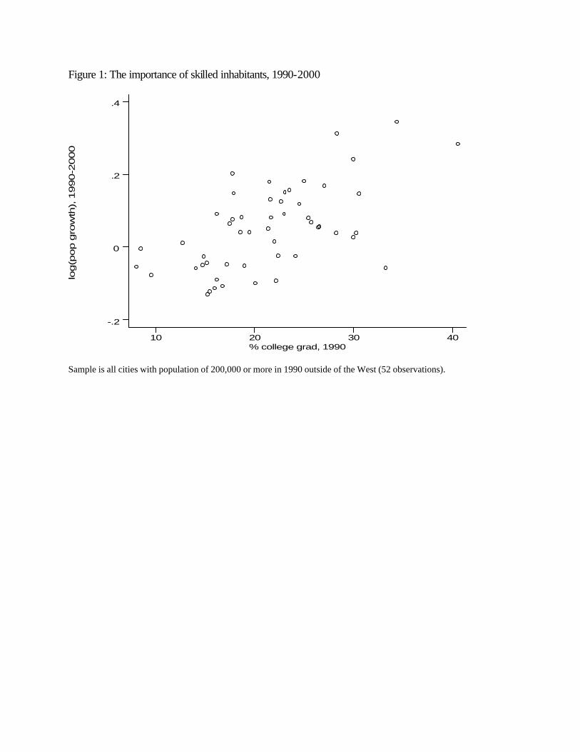
Figure 1: The importance of skilled inhabitants, 1990-2000 lo

g(p

op g

row

th), 1

990-2

000

% college grad, 199010 20 30 40

-.2

0

.2

.4

Sample is all cities with population of 200,000 or more in 1990 outside of the West (52 observations).

38

Figure 2: Persistence in city growth rates, 1980-2000 lo

g(p

op g

row

th), 1

990-2

000

log(pop growth), 1980-1990-.5 0 .5 1

-.2

0

.2

.4

.6

Sample is all cities with population of 100,000 or more in 1990 and available population data for 1980 (193 observations).

39

Figure 3: Growth and initial population, 1990-2000

log(p

op g

row

th), 1

990-2

000

log(pop), 199012 14 16

-.2

0

.2

.4

.6

Sample is all cities with population of 100,000 or more in 1990 (195 observations).

40

Figure 4: Growth and health services, 1990-2000

log(p

op g

row

th), 1

990-2

000

% health services, 19905 10 15 20

-.2

0

.2

.4

.6


41

Figure 5: Growth and poverty, 1990-2000 lo

g(p

op g

row

th), 1

990-2

000

% poor, 19890 10 20 30 40

-.2

0

.2

.4

.6


42

Data Appendix

Panel A: Cities, 1990-2000

From the County and City Data Book 1994 we obtained data on all U.S. cities for the beginning

of the 1990s. We then dropped all cities with fewer than 100,000 residents in 1990 to obtain our

final sample of 195 cities. We obtained data on population in 2000 for these 195 cities from the

U.S. Census.6 Definitions of Northeast, West, Midwest, and South regions are from the U.S.

Census. Data on 1980 population used to calculate the growth rate during the 1980s are also

from the County and City Data Book 1994. Data on 1980 populations for Moreno Valley,

California and Santa Clarita, California were not available. Complete documentation and details

on original sources are available in the County and City Data Book 1994.

Panel B: Cities, 1980-1990

From the County and City Data Book 1983 we obtained data on all U.S. cities for the beginning

of the 1980s. We then dropped all cities with fewer than 100,000 residents in 1980 to obtain our

final sample of 170 cities. We obtained data on population in 1990 for these 170 cities from the

County and City Data Book 1994. Data on 1970 population used to calculate the growth rate

during the 1970s are from the County and City Data Book 1983. Data on city government

spending per capita and spending composition for the 1980-1981 fiscal year were not available

for Honolulu, Hawaii.

Panel C: MSAs, 1990-2000.

From USA Counties 1998 we obtained a list of the counties comprising each MSA as of 1998.

We used these definitions for both 1990 and 2000 to ensure a consistent definition of each entity.

We obtained county populations for 2000 from the U.S. Census and aggregated over the counties

in each MSA to obtain MSA population in 2000.7 MSA population in 1990, MSA population in

1980, and all other MSA variables were obtained by a similar aggregation except as noted below.

We dropped all MSAs with fewer than 100,000 residents in 1990 to obtain our final sample of

6 As of June 2001 such data are accessible at http://blue.census.gov/population/www/cen2000/phc-t5.html. 7 As of June 2001 county populations can be obtained from http://blue.census.gov/population/www/cen2000/phc-t4.html.

43

251 MSAs. For each MSA in our sample, the major component city was identified and merged

with data on:

• Census-defined regions.

• Climate data from the County and City Data Book 1994.

A list of each MSA and its identified major city is available on request from Jesse Shapiro at

[email protected].

Harvard Institute of Economic...

Documents

Transcript of Harvard Institute of Economic...