HARMONY SEARCH ALGORITHM FOR SOLVING TWO AGGREGATE...

PROCEEDINGS OF THE 8th INTERNATIONAL MANAGEMENT CONFERENCE

"MANAGEMENT CHALLENGES FOR SUSTAINABLE DEVELOPMENT", November 6th-7th, 2014, BUCHAREST, ROMANIA

HARMONY SEARCH ALGORITHM FOR SOLVING TWO AGGREGATE

PRODUCTION PLANNING MODELS WITH BREAKDOWNS AND MAINTENANCE

Esmaeil MEHDIZADEH 1 Amir Aydin Atashi ABKENAR2

ABSTRACT

Aggregate Production planning (APP) and preventive maintenance (PM) are most important issue

carried out in manufacturing environments which seeks efficient planning, scheduling and

coordination of all production activities that optimizes the company's objectives. In this paper, we

develop two mixed integer linear programming (MILP) models for an integrated aggregate

production planning system with return products, breakdowns and preventive maintenance. The

goal is to minimize production breakdowns and Preventive maintenance costs and instabilities in

the work force, inventory levels and downtimes, also effect of PM on the objective function.

Additionally, Taguchi method is conducted to calibrate the parameter of the meta-heuristic and

select the optimal levels of the algorithm’s performance influential factors. Due to NP-hard class

of APP, we implement a harmony search (HS) algorithm for solving these models. Finally,

computational results show that, the objective values obtained by APP with PM are better from

APP with breakdowns results.

KEYWORDS: Harmony search, Aggregate production planning, Preventive maintenance,

Taguchi method

JEL CLASSIFICATION: D24

1. INTRODUCTION

Aggregate production planning belongs to a class of production planning problems in which there is

a single production variable representing the total production of all products (Dilworth, 1993). APP

is a medium range capacity planning method that typically encompasses a time horizon anywhere

from 2 to 18 months. The aims of APP are to set overall production levels for each product category

to meet fluctuating or uncertain demand in the near future and to set decisions concerning hiring,

layoffs, overtime, backorders, subcontracting, inventory level and determining appropriate

resources to be used (Wang and Liang, 2004).

A survey of models and methodologies for APP has been represented by Nam and Ogendar (1992).

Ashayeri et al. proposed a model optimizing total maintenance and production costs in discrete

multi-machine environment with deterministic demand (Ashayeri et al., 1995). This paper proposes

and discusses models to generate such integrated APP and maintenance plans which aim at

achieving an optimal trade-off between the various production and maintenance costs. At the

tactical level, there are only few papers discussing this issue. Wienstein and Chung presented a

three-part model to resolve the conflicting objectives of system reliability and profit maximization.

An aggregate production plan is first generated, and then a master production schedule is developed

1 Faculty of Industrial and Mechanical Engineering, Qazvin Branch, Islamic Azad University, Qazvin, Iran, [email protected] 2 Faculty of Industrial and Mechanical Engineering, Qazvin Branch, Islamic Azad University, Qazvin, Iran, [email protected]

306

mailto:[email protected]

mailto:[email protected]



to minimize the weighted deviations from the specified aggregate production goals. Finally, work

center loading requirements, determined through rough cut capacity planning, are used to simulate

equipment failures during the aggregate planning horizon. Several experiments are used to test the

significance of various factors for maintenance policy selection. These factors include the category

of maintenance activity, maintenance activity frequency, failure significance, maintenance activity

cost, and aggregate production policy (Wienstein & Chung, 1999). Sortrakul et al. proposed an

integrated maintenance planning and production scheduling model for a single machine minimizing

the total weighted expected completion time to find the optimal PM actions and job sequence

(Sortrakul et al., 2005). Aghezzaf and Najid discuss the issue of integrating production planning and

preventive maintenance in manufacturing production systems. In particular, it tackles the problem

of integrating production and preventive maintenance in a system composed of parallel failure-

prone production lines. It is assumed that when a production line fails, a minimal repair is carried

out to restore it to an ‘as-bad-as-old’ status. Preventive maintenance is carried out, periodically at

the discretion of the decision maker, to restore the production line to an ‘as-good-as-new’ status. It

is also assumed that any maintenance action, performed on a production line in a given period,

reduces the available production capacity on the line during that period (Aghezzaf & Najid, 2008).

Nourelfath and Chatelet paper deals with the problem of integrating preventive maintenance and

tactical production planning, for a production system composed of a set of parallel components, in

the presence of economic dependence and common cause failures. Economic dependence means

that performing maintenance on several components jointly costs less money and time than on each

component separately. Common cause failures correspond to events that lead to simultaneous

failure of multiple components due to a common cause (Nourelfath & Chatelet, 2012). Fitouhi and

Nourelfath developed a model for planning production and noncyclical preventive maintenance

simultaneously for a single machine, subjected to random failures and minimal repairs. The

proposed model determines simultaneously the optimal production plan and the instants of

preventive maintenance actions. The objective is to minimize the sum of preventive and corrective

maintenance costs, setup costs, holding costs, backorder costs and production costs, while satisfying

the demand for all products over the entire horizon. The problem is solved by comparing the results

of several multi-product capacitated lot-sizing problems. The value of the integration and that of

using noncyclical preventive maintenance when the demand varies from one period to another are

illustrated through a numerical example and validated by a design of experiment. The later has

shown that the integration of maintenance and production planning can reduce the total

maintenance and production cost and the removal of periodicity constraint is directly affected by the

demand fluctuation and can also reduce the total maintenance and production cost (Fitouhi &

Nourelfath, 2012). Fitouhin and Nourelfath presented an integrated model for production and

general preventive maintenance planning for multi-state systems. For the production side, the model

generates, for each product and each production planning period, the quantity of inventory,

backorder, items to produce and also the instant of set-up. For the maintenance side, for each

component, we proposed the instant of each preventive maintenance action which can be carried out

during the production planning period. A Matrix based methodology was used in order to estimate

model parameters such as system availability and the general capacity. The proposed model was

solved by the ES method and SA (Fitouhin & Nourelfath, 2014). The large part of the production

planning models assumes that the system will function at its maximum performance during the

planning horizon, and the large part of the maintenance planning models disregards the impact of

maintenance on the production capacity and does not explicitly consider the production

requirements (Aghezzaf et al., 2007). It is therefore crucial that both production and maintenance

aspects related to a production system are concurrently considered during the elaboration of optimal

production and maintenance plans. The purpose of this paper is to develop a combined production

planning model for two phase production systems, breakdowns and preventive maintenance in an

aggregate production planning. The main objective of the proposed models are to determine an

307



integrated production and maintenance plan that minimizes the expected total production and

maintenance costs over a planning horizon and effect of preventive maintenance on the aggregate

production planning model.

The remaining of this paper is organized as follows: Section 2 describes an aggregate production

planning Model with machine breakdowns, and a MILP formulation of the aggregate production

planning Model with preventive maintenance. The solution approach harmony search (HS) is

presented in Section 3. Section 4 presents computational experiments. The conclusions and

suggestions for future studies are included in Section 5.

2. The mathematical models

2.1. The APP model and breakdowns

In this section, we present an aggregate production planning model with machine breakdowns. This

model is relevant to multi-period, multi-product, multi-machine, two-phase production systems.

2.1.1. Assumptions

The quantity shortage at the beginning of the planning horizon is zero

The quantity shortage at the end of the planning horizon is zero

Breakdown decision variable, if setup to be performed, the decision variable is equal to one,

and otherwise it is zero.

There is a setup cost of producing a product only once at the beginning of a period, and the

setup cost after a failure is not considered.

2.1.2. Model variables

Pi2t: Regular time production of second-phase product i in period t units).

Oi2t: Over time production of second-phase product i in period t (units).

Ci2t: Subcontracting volume of second-phase product i in period t (units).

Bi2t: Backorder level of second-phase product i in period t (units).

Ii2t: The inventory of second-phase product i in period t (units).

Ht: The number of second group workers hired in period t (man-days).

Lt: The number of second group workers laid off in period t (man-days).

Wt: Second workforce level in period t (man-days).

Yi2t: The setup decision variable of second-phase product i in period t, a binary integer variable.

XRi2t: The number of second-phase returned products of product i that remanufactured in period t.

XRIi2t: The number of second-phase returned products of product i held that in inventory at the end

of period t.

XDi2t: The number of second-phase returned products of product i that disposed in period t.

Pk1t: Regular time production of first-phase product k in period t units).

Ok1t: Over time production of first-phase product k in period t (units).

Ck1t: Subcontracting volume of first-phase product k in period t (units).

Bk1t: Backorder level of first-phase product k in period t (units).

Ik1t: The inventory of first-phase product k in period t (units).

H't: The number of first group workers hired in period t (man-days).

L't: The number of first group workers laid off in period t (man-days).

W't: First workforce level in period t (man-days).

Yk1t: The setup decision variable of first-phase product k in period t, a binary integer variable.

308



2.1.3. Parameters

pk1t: Regular time production cost of first-phase product k in period t ($/units).

ok1t: Over time production cost of first -phase product k in period t ($/units).

ck1t: Subcontracting cost of first-phase product k in period t ($/units).

hk1t: Inventory cost of first-phase product k in period t ($/units).

ak1l: Hours of machine l per unit of first-phase product k (machine-days/unit).

uk1l: The setup time for first-phase product k on machine l (hours).

rk1lt: The setup cost of first-phase product k on machine l in period t ($/machine-hours).

R'kt: The regular time capacity of machine l in period t (machine-hours).

hr't: Cost to hire one worker in period t for first group labor ($/man-days).

l't: Cost to layoff one worker of first group in period t ($/man-days).

w't: The first group labor cost in period t ($/man-days).

Ik10: The initial inventory level of first-phase product k in period t (units).

w'0: The initial first group workforce level (man-days).

Bk10: The initial first group backorder level (man-days).

ek1: Hours of labor per unit of first-phase product k (man-days/unit).

α't: The ratio of regular-time of first group workforce available for use in overtime in period t.

β'lt: The ratio of regular time capacity of machine l available for use in overtime in period t.

w'max t: Maximum level of first group labor available in period t (man-days).

Di2t: Forecasted demand of second-phase product i in period t (units).

pi2t: Regular time production cost of second-phase product i in period t ($/units).

oi2t: Over time production cost of second-phase product i in period t ($/units).

ci2t: Subcontracting cost of second-phase product i in period t ($/units).

hi2t: Inventory cost of second-phase product i in period t ($/units).

ai2j: Hours of machine j per unit of second-phase product i (machine-days/unit).

ui2j: The setup time for second-phase product i on machine j (hours).

ri2jt: The setup cost of second-phase product i on machine j in period t ($/machine-hours).

Rjt: The regular time capacity of machine j in period t (machine-hours).

hrt: Cost to hire one worker in period t for second group labor ($/man-days).

lt: Cost to layoff one worker of second group in period t ($/man-days).

wt: The first group labor cost in period t ($/man-days).

Ii20: The initial inventory level of second-phase product i in period t (units).

w0: The initial second group workforce level (man-days).

Bi20: The initial second group backorder level (man-days).

ei2: Hours of labor per unit of second-phase product i (man-days/unit).

αt: The ratio of regular-time of second group workforce available for use in overtime in period t.

βjt: The ratio of regular time capacity of machine j available for use in overtime in period t.

f: The working hours of labor in each period (man-hour/man-day).

wmax t: Maximum level of second group labor available in period t (man-days).

Cmax it: Maximum subcontracted volume available of second-phase product i in period t (units).

fik: The number of unit of first-phase product k required per unit of first-phase product i.

TRi2t: The number of second-phase returned products of product i in period t.

XDmax i2t: The maximum number of second-phase returned products of product i that could be

disposed in period t.

XRmax i2t: The maximum number of second-phase returned products of product i that could be

remanufactured in period t.

hXi2t: Inventory cost of second-phase returned products of product i in period t ($/units).

C1l1t Failure cost of first-phase machine l in period t ($).

C3j2t Failure cost of second-phase machine j in period t ($).

C5i2t The cost of returned products of second-phase product i that disposed in period t ($).

309



C6i2t The cost of returned products of second-phase product i that remanufactured in period t ($).

m Percentage of machine capacity in each period (due to lack of maintenance in the previous

period) is lost due to Failure.

LT Lead time.

M: A large number.

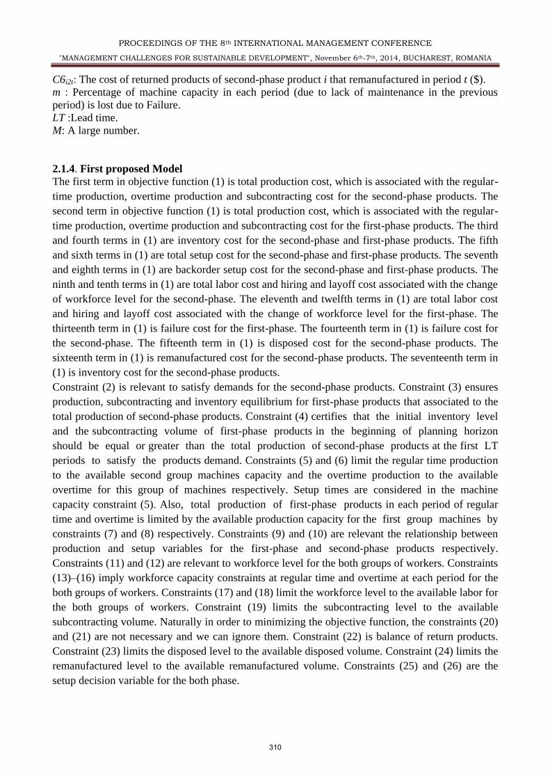
2.1.4. First proposed Model

The first term in objective function (1) is total production cost, which is associated with the regular-

time production, overtime production and subcontracting cost for the second-phase products. The

second term in objective function (1) is total production cost, which is associated with the regular-

time production, overtime production and subcontracting cost for the first-phase products. The third

and fourth terms in (1) are inventory cost for the second-phase and first-phase products. The fifth

and sixth terms in (1) are total setup cost for the second-phase and first-phase products. The seventh

and eighth terms in (1) are backorder setup cost for the second-phase and first-phase products. The

ninth and tenth terms in (1) are total labor cost and hiring and layoff cost associated with the change

of workforce level for the second-phase. The eleventh and twelfth terms in (1) are total labor cost

and hiring and layoff cost associated with the change of workforce level for the first-phase. The

thirteenth term in (1) is failure cost for the first-phase. The fourteenth term in (1) is failure cost for

the second-phase. The fifteenth term in (1) is disposed cost for the second-phase products. The

sixteenth term in (1) is remanufactured cost for the second-phase products. The seventeenth term in

(1) is inventory cost for the second-phase products.

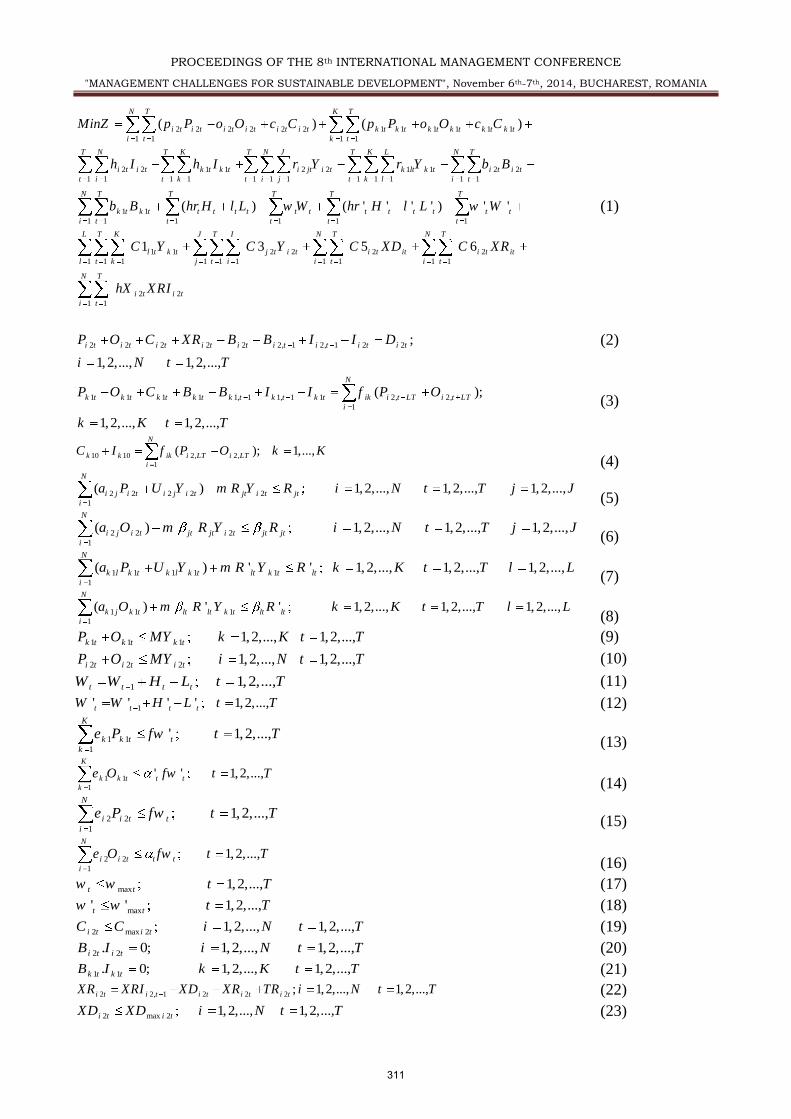
Constraint (2) is relevant to satisfy demands for the second-phase products. Constraint (3) ensures

production, subcontracting and inventory equilibrium for first-phase products that associated to the

total production of second-phase products. Constraint (4) certifies that the initial inventory level

and the subcontracting volume of first-phase products in the beginning of planning horizon

should be equal or greater than the total production of second-phase products at the first LT

periods to satisfy the products demand. Constraints (5) and (6) limit the regular time production

to the available second group machines capacity and the overtime production to the available

overtime for this group of machines respectively. Setup times are considered in the machine

capacity constraint (5). Also, total production of first-phase products in each period of regular

time and overtime is limited by the available production capacity for the first group machines by

constraints (7) and (8) respectively. Constraints (9) and (10) are relevant the relationship between

production and setup variables for the first-phase and second-phase products respectively.

Constraints (11) and (12) are relevant to workforce level for the both groups of workers. Constraints

(13)–(16) imply workforce capacity constraints at regular time and overtime at each period for the

both groups of workers. Constraints (17) and (18) limit the workforce level to the available labor for

the both groups of workers. Constraint (19) limits the subcontracting level to the available

subcontracting volume. Naturally in order to minimizing the objective function, the constraints (20)

and (21) are not necessary and we can ignore them. Constraint (22) is balance of return products.

Constraint (23) limits the disposed level to the available disposed volume. Constraint (24) limits the

remanufactured level to the available remanufactured volume. Constraints (25) and (26) are the

setup decision variable for the both phase.

310



2 2 2 2 2 2 1 1 1 1 1 1

1 1 1 1

2 2 1 1 2 2 1 1 2 2

1 1 1 1 1 1 1 1 1 1 1 1

1 1

( ) ( )N T K T

i t i t i t i t i t i t k t k t k t k t k t k t

i t k t

T N T K T N J T K L N T

i t i t k t k t i jt i t k lt k t i t i t

t i t k t i j t k l i t

k t k t

t

MinZ p P o O c C p P o O c C

h I h I r Y r Y b B

b B1 1 1 1 1 1

1 1 2 2 2 2

1 1 1 1 1 1 1 1 1 1

2 2

1 1

( ) ( ' ' ' ' ) ' '

1 3 5 6

N T T T T T

t t t t t t t t t t t t

i t t t t

L T K J T I N T N T

l t k t j t i t i t it i t it

l t k j t i i t i t

N T

i t i t

i t

hr H l L w W hr H l L w W

C Y C Y C XD C XR

hX XRI

(1)

2 2 2 2 2 2, 1 2, 1 2 2 ;

1,2,..., 1,2,...,

i t i t i t i t i t i t i t i t i tP O C XR B B I I D

i N t T

(2)

2,1 1 1 1 1, 1 1 ,, 2

1

1 1

1,

( )

2,..., 1,2,.. ,

;

.

N

ik i tk t k t k t k t k t k LT i t Lt k t T

i

P O C B B fI I

k K t

P O

T

(3)

2,10 2,

1

10 1,.( ) ,; ..N

ik i LT i LT

i

k kC I kf KP O

(4)

2

1

22 2 2 1,2,..., 1,2,..., 1,2,..( ) .,N

i j i t i j i t jjt i t

i

tR Y i N ta P U Y jR Jm T

(5)

2

1

22 1,2,..., 1,2,..., 1,2, .( ) .. ,jt jt

N

i j i t jt jt

i

i ta O m RR Y i N t T j J

(6)

1 1 1 11

1

' 1,2,..., 1,2,..., 1,2,...,( ) 'lt

N

k l k t k l k t ltk t

i

R Y k K t T l La P U Y m R

(7)

1

11 1 ' 1,2,..., 1,2,..., 1,( ) ' 2,...,N

k j k t ltlt l

i

k tlt tR Y k K t T la O m LR

(8)

1 1 1 1,2,..., 1,2,...,k t k t k tP O MY K Tk t (9)

2 2 2 1,2,..., 1,2,...,i t i t i tP O MY i N t T (10)

1 1,2,...,t t t tW W H L t T (11)

1' ' ' ' 1,2,...,t t t tW W H L t T (12)

1 1

1

1,2,...,'K

k k t t

k

e P fw t T

(13)

1 1

1

1,2,..' ' .,K

k k t t t

k

e O fw t T

(14)

2 2

1

1,2,...,N

i i t t

i

e P Tw tf

(15)

2 2

1

1,2,...,N

i i t t t

i

t Te O fw

(16)

max 1,2,...,t t tw Tw (17)

max 1,2,...,' 't tw w t T (18)

2 max 2 1,2,..., 1,2,...,i t i tC C i N t T (19)

2 2 1,2. ,..., 1,20; ,...,i t i tB I i N t T (20)

1 1 1,2,..., 1,2,.. 0 ,; ..k t k tB I k K t T (21)

2 2, 1 2 2 2 ; 1,2,..., 1,2,...,i t i t i t i t i tXR XRI i N t TXD XR TR (22)

2 max 2 1,2,..., 1,2,...,i t i t iX XD t TD N (23)

311



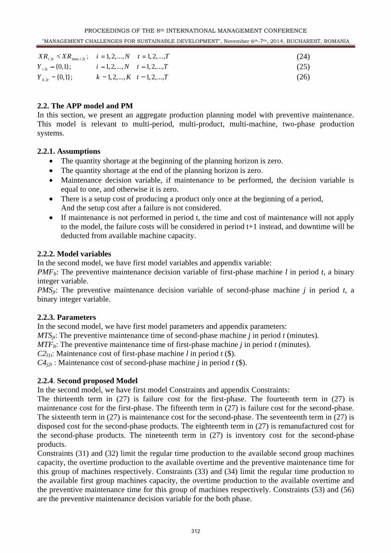
2 max 2 1,2,..., 1,2,...,i t i t i N tXR XR T (24)

2 {0,1}; 1,2,..., 1,2,...,i tY i N t T (25)

2 {0,1}; 1,2,..., 1,2,...,k tY k K t T (26)

2.2. The APP model and PM

In this section, we present an aggregate production planning model with preventive maintenance.

This model is relevant to multi-period, multi-product, multi-machine, two-phase production

systems.

2.2.1. Assumptions

The quantity shortage at the beginning of the planning horizon is zero

The quantity shortage at the end of the planning horizon is zero

Maintenance decision variable, if maintenance to be performed, the decision variable is

equal to one, and otherwise it is zero.

There is a setup cost of producing a product only once at the beginning of a period,

And the setup cost after a failure is not considered.

If maintenance is not performed in period t, the time and cost of maintenance will not apply

to the model, the failure costs will be considered in period t+1 instead, and downtime will be

deducted from available machine capacity.

2.2.2. Model variables

In the second model, we have first model variables and appendix variable:

PMFlt: The preventive maintenance decision variable of first-phase machine l in period t, a binary

integer variable.

PMSjt: The preventive maintenance decision variable of second-phase machine j in period t, a

binary integer variable.

2.2.3. Parameters

In the second model, we have first model parameters and appendix parameters:

MTSjt: The preventive maintenance time of second-phase machine j in period t (minutes).

MTFlt: The preventive maintenance time of first-phase machine j in period t (minutes).

C2l1t Maintenance cost of first-phase machine l in period t ($).

C4j2t Maintenance cost of second-phase machine j in period t ($).

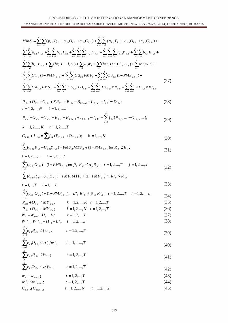
2.2.4. Second proposed Model

In the second model, we have first model Constraints and appendix Constraints:

The thirteenth term in (27) is failure cost for the first-phase. The fourteenth term in (27) is

maintenance cost for the first-phase. The fifteenth term in (27) is failure cost for the second-phase.

The sixteenth term in (27) is maintenance cost for the second-phase. The seventeenth term in (27) is

disposed cost for the second-phase products. The eighteenth term in (27) is remanufactured cost for

the second-phase products. The nineteenth term in (27) is inventory cost for the second-phase

products.

Constraints (31) and (32) limit the regular time production to the available second group machines

capacity, the overtime production to the available overtime and the preventive maintenance time for

this group of machines respectively. Constraints (33) and (34) limit the regular time production to

the available first group machines capacity, the overtime production to the available overtime and

the preventive maintenance time for this group of machines respectively. Constraints (53) and (56)

are the preventive maintenance decision variable for the both phase.

312



2 2 2 2 2 2 1 1 1 1 1 1

1 1 1 1

2 2 1 1 2 2 1 1 2 2

1 1 1 1 1 1 1 1 1 1 1 1

1 1

( ) ( )N T K T

i t i t i t i t i t i t k t k t k t k t k t k t

i t k t

T N T K T N J T K L N T

i t i t k t k t i jt i t k lt k t i t i t

t i t k t i j t k l i t

k t k t

t

MinZ p P o O c C p P o O c C

h I h I r Y r Y b B

b B1 1 1 1 1 1

1

1 , 1 1 2 , 1

1 1 1 0 1 1

1

2 2 2

1 0 1 1 1

( ) ( ' ' ' ' ) ' '

1 (1 ) 2 3 (1 )

4 5

N T T T T T

t t t t t t t t t t t t

i t t t t

L T L T J T

l t l t l t lt j t j t

l t l t j t

J T N T T

j t jt i t i t

l t i t i t

hr H l L w W hr H l L w W

C PMF C PMF C PMS

C PMS C XD 2 2 2 2

1 1 1

6N N T

i t i t i t i t

i t

C XR hX XRI

(27)

2 2 2 2 2 2, 1 2, 1 2 2 ;

1,2,..., 1,2,...,

i t i t i t i t i t i t i t i t i tP O C XR B B I I D

i N t T

(28)

2,1 1 1 1 1, 1 1 ,, 2

1

1 1

1,

( )

2,..., 1,2,.. ,

;

.

N

ik i tk t k t k t k t k t k LT i t Lt k t T

i

P O C B B fI I

k K t

P O

T

(29)

2,10 2,

1

10 1,.( ) ,; ..N

ik i LT i Lk

i

k TC I k Kf P O

(30)

,2 2 2 2

1

1(1 )

1,2,..., 1, 2

( )

,...,

N

i j i t i jt jt jj i t jt

i

t jta P U Y mPMS MTS PMS R

t T j

R

J

(31)

2 , 12

1

(1 ) 1,2,..., 1,2,.. ,( ) .j t j

N

i j i t jt jt tjt

i

PMS R t Ta O jm R J

(32)

,

1

11 1 1 1 (1 ) '

1,..

( ) '

., 1,...,

lt lt l t l

N

k l k t k l t tk lt

i

a PMF MTF PMF R

t T l

P

L

U Y m R

(33)

1 , 11

1

(1 ) ' ' ' 1,2,..., 1,2,.) ..( ' ,l t l

N

k j k t lt lt

i

t ltPMF R t T l La O m R

(34)

1 1 1 1,2,..., 1,2,...,k t k t k tP O MY K Tk t (35)

2 2 2 1,2,..., 1,2,...,i t i t i tP O MY i N t T (36)

1 1,2,...,t t t tW W H L t T (37)

1' ' ' ' 1,2,...,t t t tW W H L t T (38)

1 1

1

1,2,.' ; ..,K

k k t t

k

e P fw t T

(39)

1 1

1

;' 1,2,..' .,K

k k t t t

k

e O fw t T

(40)

2 2

1

; 1,2,...,N

i i t t

i

e P fw t T

(41)

2 2

1

1,2,...,N

i i t t t

i

O w Te f t

(42)

max 1,2,...,t tw w t T (43)

max 1,2,...,' 't tw w t T (44)

2 max 2 1,2,..., 1,2,...,i t i tC C i N t T (45)

313



2 2 1,2,..., 1,2,...,. 0i t i t i N t TB I (46)

1 1 1,2,..., 1. 0 ,2,...,;k t k t K tB I k T (47)

2 2, 1 2 2 2 ; 1,2,..., 1,2,...,i t i t i t i t i tXR XRI XD XR i N t TTR (48)

2 max 2 1,2,..., 1,2,...,i t i t iXD XD N t T (49)

2 max 2 1,2,..., 1,2,...,i t i t iXR XR N t T (50)

2 {0,1}; 1,2,..., 1,2,...,i tY i N t T (51)

2 {0,1}; 1,2,..., 1,2,...,k tY k K t T (52)

{0,1}; 1,2,..., 1,2,...,ltPMF l L t T (53)

{0,1}; 1,2,..., 1,2,...,jtPMS j J t T (54)

0 1; 1,2,...,lPMF l L (55)

0 1; 1,2,...,jPMS j J (56)

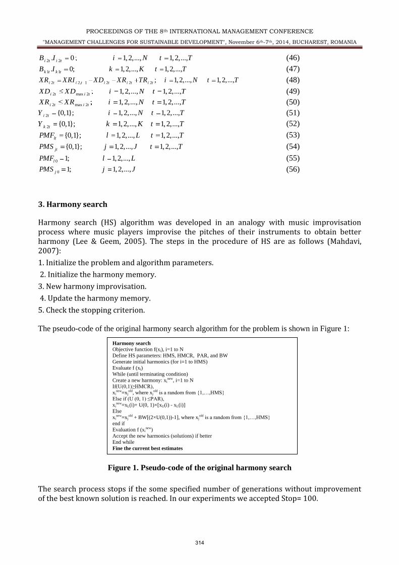
3. Harmony search

Harmony search (HS) algorithm was developed in an analogy with music improvisation process where music players improvise the pitches of their instruments to obtain better harmony (Lee & Geem, 2005). The steps in the procedure of HS are as follows (Mahdavi, 2007):

1. Initialize the problem and algorithm parameters.

2. Initialize the harmony memory.

3. New harmony improvisation.

4. Update the harmony memory.

5. Check the stopping criterion.

The pseudo-code of the original harmony search algorithm for the problem is shown in Figure 1:

Figure 1. Pseudo-code of the original harmony search

The search process stops if the some specified number of generations without improvement of the best known solution is reached. In our experiments we accepted Stop= 100.

Harmony search

Objective function f(xi), i=1 to N

Define HS parameters: HMS, HMCR, PAR, and BW

Generate initial harmonics (for i=1 to HMS)

Evaluate f (xi)

While (until terminating condition)

Create a new harmony: xinew, i=1 to N

If(U(0,1)≥HMCR),

xinew=xj

old, where xjold is a random from {1,…,HMS}

Else if (U (0, 1) ≤PAR),

xinew=xL(i)+ U(0, 1)×[xU(i) - xL(i)]

Else

xinew=xj

old + BW[(2×U(0,1))-1], where xjold is a random from {1,…,HMS}

end if

Evaluation f (xinew)

Accept the new harmonics (solutions) if better

End while

Fine the current best estimates

314



4. Results

In order to evaluate the performance of the meta-heuristic algorithms, 30 test problems with

different sizes are randomly generated for each model. The proposed models are coded with

LINGO 8 software and using LINGO solver for solving the instances. Furthermore, for the small

and medium sized instances of two phases APP with breakdown and PM, LINGO optimization

solver is used to figure out the optimal solution and compared with HS results.

The proposed algorithm was programmed in MATLAB R2011a and all tests are conducted on a not

book at Intel Core 2 Duo Processor 2.00 GHz and 2 GB of RAM.

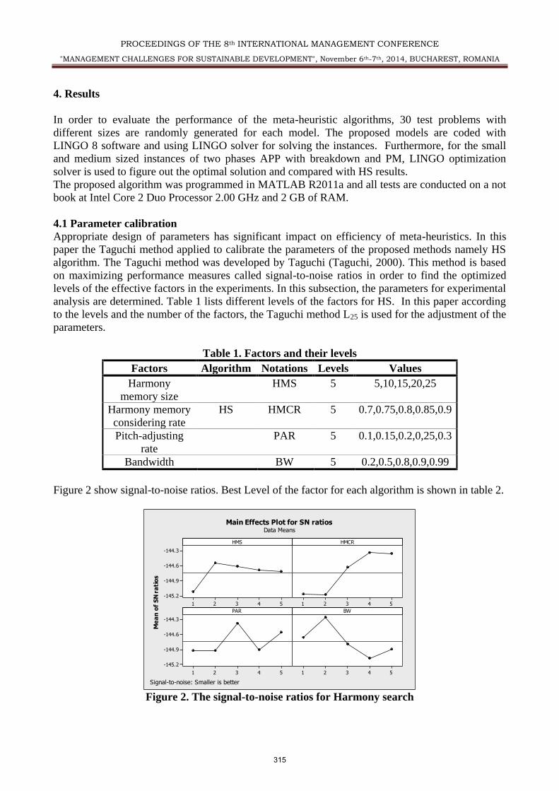
4.1 Parameter calibration

Appropriate design of parameters has significant impact on efficiency of meta-heuristics. In this

paper the Taguchi method applied to calibrate the parameters of the proposed methods namely HS

algorithm. The Taguchi method was developed by Taguchi (Taguchi, 2000). This method is based

on maximizing performance measures called signal-to-noise ratios in order to find the optimized

levels of the effective factors in the experiments. In this subsection, the parameters for experimental

analysis are determined. Table 1 lists different levels of the factors for HS. In this paper according

to the levels and the number of the factors, the Taguchi method L25 is used for the adjustment of the

parameters.

Table 1. Factors and their levels

Factors Algorithm Notations Levels Values

Harmony

memory size

HMS 5 5,10,15,20,25

Harmony memory

considering rate

HS HMCR 5 0.7,0.75,0.8,0.85,0.9

Pitch-adjusting

rate

PAR 5 0.1,0.15,0.2,0,25,0.3

Bandwidth BW 5 0.2,0.5,0.8,0.9,0.99

Figure 2 show signal-to-noise ratios. Best Level of the factor for each algorithm is shown in table 2.

54321

-144.3

-144.6

-144.9

-145.2

54321

54321

-144.3

-144.6

-144.9

-145.2

54321

HMS

Me

an

of

SN

ra

tio

s

HMCR

PAR BW

Main Effects Plot for SN ratiosData Means

Signal-to-noise: Smaller is better

Figure 2. The signal-to-noise ratios for Harmony search

315



Table 2. Best level for parameters

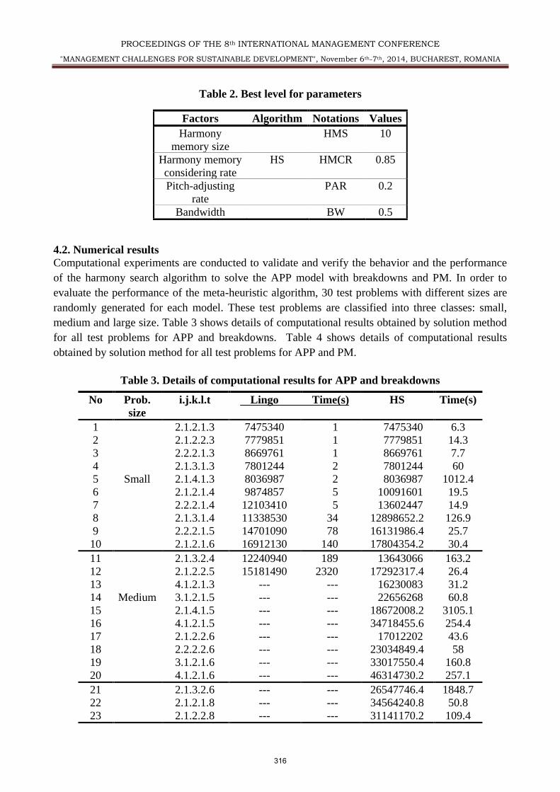
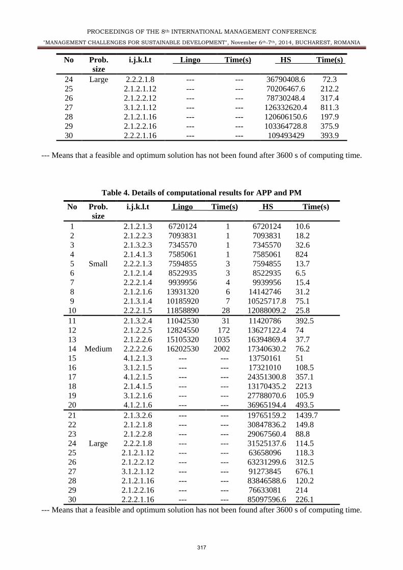
4.2. Numerical results

Computational experiments are conducted to validate and verify the behavior and the performance

of the harmony search algorithm to solve the APP model with breakdowns and PM. In order to

evaluate the performance of the meta-heuristic algorithm, 30 test problems with different sizes are

randomly generated for each model. These test problems are classified into three classes: small,

medium and large size. Table 3 shows details of computational results obtained by solution method

for all test problems for APP and breakdowns. Table 4 shows details of computational results

obtained by solution method for all test problems for APP and PM.

Table 3. Details of computational results for APP and breakdowns

Time(s) HS Time(s) Lingo i.j.k.l.t Prob.

size

No

6.3 7475340 1 7475340 2.1.2.1.3 1

14.3 7779851 1 7779851 2.1.2.2.3 2

7.7 8669761 1 8669761 2.2.2.1.3 3

60 7801244 2 7801244 2.1.3.1.3 4

1012.4 8036987 2 8036987 2.1.4.1.3 Small 5

19.5 10091601 5 9874857 2.1.2.1.4 6

14.9 13602447 5 12103410 2.2.2.1.4 7

126.9 12898652.2 34 11338530 2.1.3.1.4 8

25.7 16131986.4 78 14701090 2.2.2.1.5 9

30.4 17804354.2 140 16912130 2.1.2.1.6 10

163.2 13643066 189 12240940 2.1.3.2.4 11

26.4 17292317.4 2320 15181490 2.1.2.2.5 12

31.2 16230083 --- --- 4.1.2.1.3 13

60.8 22656268 --- --- 3.1.2.1.5 Medium 14

3105.1 18672008.2 --- --- 2.1.4.1.5 15

254.4 34718455.6 --- --- 4.1.2.1.5 16

43.6 17012202 --- --- 2.1.2.2.6 17

58 23034849.4 --- --- 2.2.2.2.6 18

160.8 33017550.4 --- --- 3.1.2.1.6 19

257.1 46314730.2 --- --- 4.1.2.1.6 20

1848.7 26547746.4 --- --- 2.1.3.2.6 21

50.8 34564240.8 --- --- 2.1.2.1.8 22

109.4 31141170.2 --- --- 2.1.2.2.8 23

Factors Algorithm Notations Values

Harmony

memory size

HMS 10

Harmony memory

considering rate

HS HMCR 0.85

Pitch-adjusting

rate

PAR 0.2

Bandwidth BW 0.5

316




size

No

72.3 36790408.6 --- --- 2.2.2.1.8 Large 24

212.2 70206467.6 --- --- 2.1.2.1.12 25

317.4 78730248.4 --- --- 2.1.2.2.12 26

811.3 126332620.4 --- --- 3.1.2.1.12 27

197.9 120606150.6 --- --- 2.1.2.1.16 28

375.9 103364728.8 --- --- 2.1.2.2.16 29

393.9 109493429 --- --- 2.2.2.1.16 30

--- Means that a feasible and optimum solution has not been found after 3600 s of computing time.

Table 4. Details of computational results for APP and PM


size

No

10.6 6720124 1 6720124 2.1.2.1.3 1

18.2 7093831 1 7093831 2.1.2.2.3 2

32.6 7345570 1 7345570 2.1.3.2.3 3

824 7585061 1 7585061 2.1.4.1.3 4

13.7 7594855 3 7594855 2.2.2.1.3 Small 5

6.5 8522935 3 8522935 2.1.2.1.4 6

15.4 9939956 4 9939956 2.2.2.1.4 7

31.2 14142746 6 13931320 2.1.2.1.6 8

75.1 10525717.8 7 10185920 2.1.3.1.4 9

25.8 12088009.2 28 11858890 2.2.2.1.5 10

392.5 11420786 31 11042530 2.1.3.2.4 11

74 13627122.4 172 12824550 2.1.2.2.5 12

37.7 16394869.4 1035 15105320 2.1.2.2.6 13

76.2 17340630.2 2002 16202530 2.2.2.2.6 Medium 14

51 13750161 --- --- 4.1.2.1.3 15

108.5 17321010 --- --- 3.1.2.1.5 16

357.1 24351300.8 --- --- 4.1.2.1.5 17

2213 13170435.2 --- --- 2.1.4.1.5 18

105.9 27788070.6 --- --- 3.1.2.1.6 19

493.5 36965194.4 --- --- 4.1.2.1.6 20

1439.7 19765159.2 --- --- 2.1.3.2.6 21

149.8 30847836.2 --- --- 2.1.2.1.8 22

88.8 29067560.4 --- --- 2.1.2.2.8 23

114.5 31525137.6 --- --- 2.2.2.1.8 Large 24

118.3 63658096 --- --- 2.1.2.1.12 25

312.5 63231299.6 --- --- 2.1.2.2.12 26

676.1 91273845 --- --- 3.1.2.1.12 27

120.2 83846588.6 --- --- 2.1.2.1.16 28

214 76633081 --- --- 2.1.2.2.16 29

226.1 85097596.6 --- --- 2.2.2.1.16 30

--- Means that a feasible and optimum solution has not been found after 3600 s of computing time.

317



1 1 1 1 1 1 1

1 10

0 10

[20,24], [22,27], [70,77], [40,45], [40,45], 1, 0.1,

[4,7], ' [21000,40000], ' [200,480], ' [200,480], ' [60,65], 500,

' 3500, 0, 0.2, 0.2, 0

k t k t k t k t k t k l k l

k lt lt t t t k

k kl t lt

p o c h h a u

r R hr l w I

w B e max 2

2 2 2 2 2 2

2 20

0

.5, [3000,7000], [6000,24000],

[20,25], [22,27], [100,106], [60,67], [0.4,0.5], 0.2,

[10,15], [21000,40000], [200,460], [200,460], [61,64], 500,

t i t

i t i t i t i t i j i j

i jt jt t t t i

w D

p o c h a u

r R hr l w I

w 20 2 max

max 1 1

2 2 2

3500, 0, 0.4, 0.2, [0.4,0.5], [120,190], [3000,7000],

[2000,9500], 2, 1 [100000,220000], 2 [10000,50000],

3 [100000,220000], 4 [10000,50000], 5 [11,14], 6

i i t jt t

it ik l t l t

j t j t i t i

B e f w

C f C C

C C C C 2

2 max 2

max 2 2 [60,65];

[4,7],

[1500,5000], [1500,5000], [300,800], [300,600],

[400,650], , 0.1, 1.

t

jt lt i t i t

i it thX

MTS MTF TR XD

XR m LT

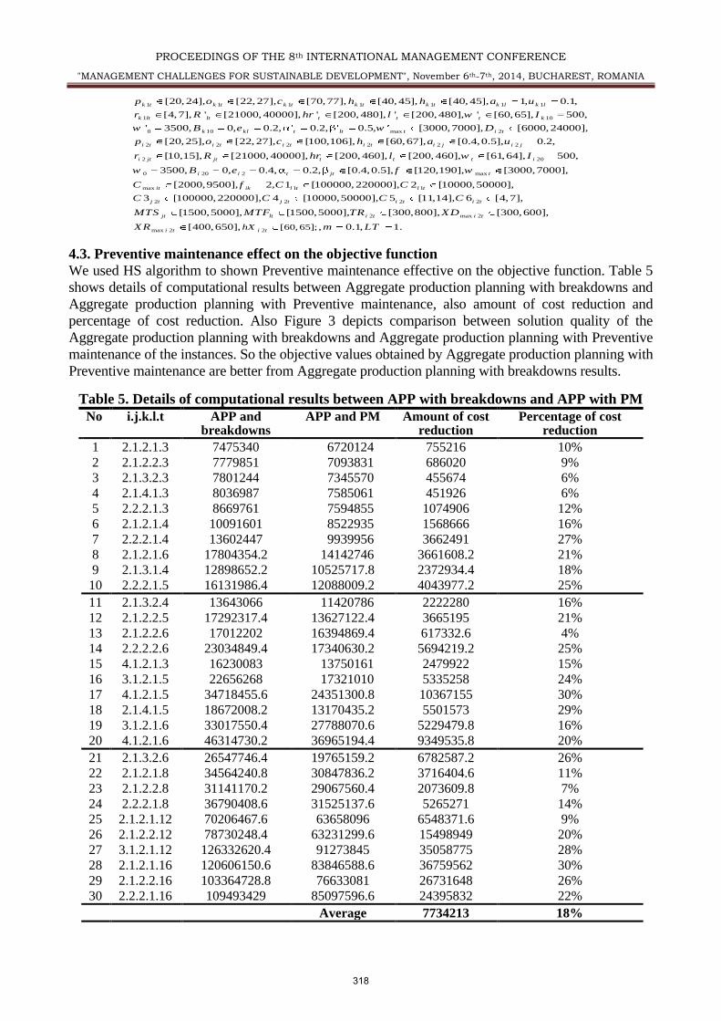
4.3. Preventive maintenance effect on the objective function

We used HS algorithm to shown Preventive maintenance effective on the objective function. Table 5

shows details of computational results between Aggregate production planning with breakdowns and

Aggregate production planning with Preventive maintenance, also amount of cost reduction and

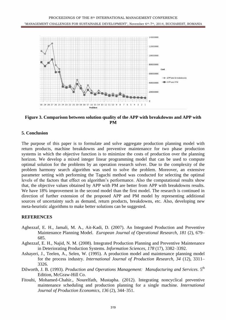
percentage of cost reduction. Also Figure 3 depicts comparison between solution quality of the

Aggregate production planning with breakdowns and Aggregate production planning with Preventive

maintenance of the instances. So the objective values obtained by Aggregate production planning with

Preventive maintenance are better from Aggregate production planning with breakdowns results.

Table 5. Details of computational results between APP with breakdowns and APP with PM

Percentage of cost reduction

Amount of cost reduction

APP and PM APP and breakdowns

i.j.k.l.t No

10% 755216 6720124 7475340 2.1.2.1.3 1

9% 686020 7093831 7779851 2.1.2.2.3 2

6% 455674 7345570 7801244 2.1.3.2.3 3

6% 451926 7585061 8036987 2.1.4.1.3 4

12% 1074906 7594855 8669761 2.2.2.1.3 5

16% 1568666 8522935 10091601 2.1.2.1.4 6

27% 3662491 9939956 13602447 2.2.2.1.4 7

21% 3661608.2 14142746 17804354.2 2.1.2.1.6 8

18% 2372934.4 10525717.8 12898652.2 2.1.3.1.4 9

25% 4043977.2 12088009.2 16131986.4 2.2.2.1.5 10

16% 2222280 11420786 13643066 2.1.3.2.4 11

21% 3665195 13627122.4 17292317.4 2.1.2.2.5 12

4% 617332.6 16394869.4 17012202 2.1.2.2.6 13

25% 5694219.2 17340630.2 23034849.4 2.2.2.2.6 14

15% 2479922 13750161 16230083 4.1.2.1.3 15

24% 5335258 17321010 22656268 3.1.2.1.5 16

30% 10367155 24351300.8 34718455.6 4.1.2.1.5 17

29% 5501573 13170435.2 18672008.2 2.1.4.1.5 18

16% 5229479.8 27788070.6 33017550.4 3.1.2.1.6 19

20% 9349535.8 36965194.4 46314730.2 4.1.2.1.6 20

26% 6782587.2 19765159.2 26547746.4 2.1.3.2.6 21

11% 3716404.6 30847836.2 34564240.8 2.1.2.1.8 22

7% 2073609.8 29067560.4 31141170.2 2.1.2.2.8 23

14% 5265271 31525137.6 36790408.6 2.2.2.1.8 24

9% 6548371.6 63658096 70206467.6 2.1.2.1.12 25

20% 15498949 63231299.6 78730248.4 2.1.2.2.12 26

28% 35058775 91273845 126332620.4 3.1.2.1.12 27

30% 36759562 83846588.6 120606150.6 2.1.2.1.16 28

26% 26731648 76633081 103364728.8 2.1.2.2.16 29

22% 24395832 85097596.6 109493429 2.2.2.1.16 30

18% 7734213 Average

318



Figure 3. Comparison between solution quality of the APP with breakdowns and APP with

PM

5. Conclusion

The purpose of this paper is to formulate and solve aggregate production planning model with

return products, machine breakdowns and preventive maintenance for two phase production

systems in which the objective function is to minimize the costs of production over the planning

horizon. We develop a mixed integer linear programming model that can be used to compute

optimal solution for the problems by an operation research solver. Due to the complexity of the

problem harmony search algorithm was used to solve the problem. Moreover, an extensive

parameter setting with performing the Taguchi method was conducted for selecting the optimal

levels of the factors that effect on algorithm’s performance. Also the computational results show

that, the objective values obtained by APP with PM are better from APP with breakdowns results.

We have 18% improvement in the second model than the first model. The research is continued in

direction of further extension of the proposed APP and PM model by representing additional

sources of uncertainty such as demand, return products, breakdowns, etc. Also, developing new

meta-heuristic algorithms to make better solutions can be suggested.

REFERENCES

Aghezzaf, E. H., Jamali, M. A., Ait-Kadi, D. (2007). An Integrated Production and Preventive

Maintenance Planning Model. European Journal of Operational Research, 181 (2), 679–

685.

Aghezzaf, E. H., Najid, N. M. (2008). Integrated Production Planning and Preventive Maintenance

in Deteriorating Production Systems. Information Sciences, 178 (17), 3382–3392.

Ashayeri, J., Teelen, A., Selen, W. (1995). A production model and maintenance planning model

for the process industry. International Journal of Production Research, 34 (12), 3311–

3326.

Dilworth, J. B. (1993). Production and Operations Management: Manufacturing and Services. 5th

Edition, McGraw-Hill Co.

Fitouhi, Mohamed-Chahir., Nourelfath, Mustapha. (2012). Integrating noncyclical preventive

maintenance scheduling and production planning for a single machine. International

Journal of Production Economics, 136 (2), 344–351.

319



Fitouhi, Mohamed-Chahir., Nourelfath, Mustapha. (2014). Integrating noncyclical preventive

maintenance scheduling and production planning for multi-state systems. Reliability

Engineering and System Safety, 121, 175–186.

Lee, K. S., Geem, Z. W. (2005). A new meta-heuristic algorithm for continuous engineering

optimization: harmony search theory and practice. Computer Methods in Applied

Mechanical Engineering, 194 (36-38), 3902–3933.

Mahdavi, M., Fesanghary, M., Damangir, E. (2007). An improved harmony search algorithm for

solving optimization problems. Applied Mathematics and Computation, 188 (2), 1567–

1579.

Nam, S. J., Ogendar, N. R. (1992). Aggregate production planning–a survey of models and

methodologies. European Journal of Operational Research, 61 (3), 255–272.

Nourelfath, M., Chatelet, E. (2012). Integrating production, inventory and maintenance planning for

a parallel system with dependent components. Reliability Engineering and System Safety,

Vol. 101, 59–66.

Sortrakul, N., Nachtmann, C., Cassady, C. (2005). Genetic algorithms for integrated preventive

maintenance planning and production scheduling for a single machine. Computers in

Industry, 56(2), 161–168.

Taguchi, G. & Chowdhury, S. (2000). Taguchi, Robust Engineering. McGraw-Hill, New York.

Wang, R. C., Liang, T. F. (2004). Application of fuzzy multi-objective linear programming to

aggregate production planning. Comput Ind Eng, 46 (1), 17–41.

Wienstein, L., Chung, C.H. (1999). Integrated maintenance and production decisions in a

hierarchical production planning environment. Computers & Operations Research, 26 (10-

11), 1059–1074.

320

HARMONY SEARCH ALGORITHM FOR SOLVING TWO AGGREGATE...

Documents

Transcript of HARMONY SEARCH ALGORITHM FOR SOLVING TWO AGGREGATE...