Harman Outline 1B CENG 5131 PDF -...
8
Harman Outline 1B CENG 5131 PDF D. Polynomials (Harman P 160) Review Harman Pages 160-161. Let a 0 ,a 1 ,...,a n be n+1 arbitrary numbers with a n = 0. Then, the function P (z)= a n z n + a n-1 z n-1 + ··· + a 0 (1) is a polynomial of degree n. The n+1 constants a 0 ,a 1 ,...,a n are the coefficients of the polynomial. A polynomial is a real polynomial if all its coefficients are real numbers. This text considers only polynomials with real coefficients unless otherwise stated, because these are associated with mathematical models of physical systems. The numbers z that are solutions to the equation P (z)=0 (2) are called the roots or sometimes the zeros of the polynomial. The values of the roots are not necessarily real numbers. Thus, a root z may have the form z = x + iy, where i is the imaginary number √ -1. In electrical engineering problems, this is often written j so that no confusion would result with the current if it is designated by i. As described in Chapter 2, the number ¯ z = x -iy is the complex conjugate of z. The notation z * is also used to designate the complex conjugate of z. 1
Transcript of Harman Outline 1B CENG 5131 PDF -...
Harman Outline 1B CENG 5131 PDF
D. Polynomials (Harman P 160)Review Harman Pages 160-161.
Let a0, a1, . . . , an be n+1 arbitrary numbers with an 6= 0. Then, the function
P (z) = anzn + an−1zn−1 + · · ·+ a0 (1)
is a polynomial of degree n. The n+1 constants a0, a1, . . . , an are the coefficientsof the polynomial. A polynomial is a real polynomial if all its coefficients arereal numbers. This text considers only polynomials with real coefficients unlessotherwise stated, because these are associated with mathematical models ofphysical systems.
The numbers z that are solutions to the equation
P (z) = 0 (2)
are called the roots or sometimes the zeros of the polynomial. The values ofthe roots are not necessarily real numbers. Thus, a root z may have the formz = x + iy, where i is the imaginary number
√−1. In electrical engineering
problems, this is often written j so that no confusion would result with thecurrent if it is designated by i. As described in Chapter 2, the number z̄ = x−iyis the complex conjugate of z. The notation z∗ is also used to designate thecomplex conjugate of z.
1
Important properties of real polynomials and their roots are as follows:
1. A polynomial of degree n ≥ 1 has n roots.
2. A polynomial of odd degree has at least one real root.
3. If z is a complex root of a real polynomial, then the complex conjugate z̄is a root also.
The polynomial P (z) = anzn + an−1zn−1 + · · · + a0 can always be written
in the formP (z) = (z − z1)(z − z2) · · · (z − zn)an (3)
as the product of linear factors using the roots zi, i = 1, 2, . . . , n of
P (z) = 0.
2
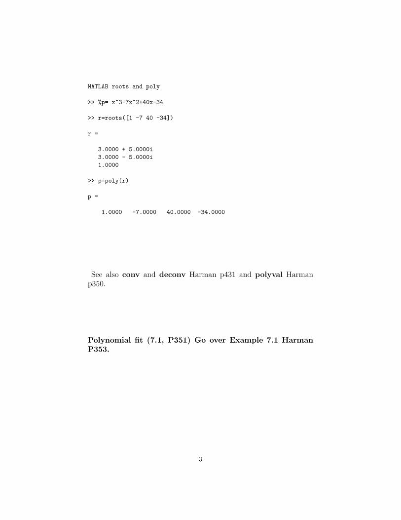
MATLAB roots and poly
>> %p= x^3-7x^2+40x-34
>> r=roots([1 -7 40 -34])
r =
3.0000 + 5.0000i3.0000 - 5.0000i1.0000
>> p=poly(r)
p =
1.0000 -7.0000 40.0000 -34.0000
See also conv and deconv Harman p431 and polyval Harmanp350.
Polynomial fit (7.1, P351) Go over Example 7.1 HarmanP353.
3
Handout 4. Functions, Sequences, Series (Harman P 276)Review Harman Pages 276-277,282-296.
1. Continuous functions definition P276
2. Sequences Section 6.2 P 282
3. Infinite Series P 284-287
4. Geometric Series P 287
5. Series of functions P 288
6. Power Series P 290
Taylor Series (6.3, P292)After a review of Taylor series, we can visit Euler’s formula againusing results in Table 6.3 P295. Consider the Taylor series
eiθ = 1 + iθ +(iθ)2
2!+
(iθ)3
3!+
(iθ)4
4!+ · · ·
Collecting terms using the fact that i2 = −1, i3 = −i, and so onyields
eiθ =
(1− (θ)2
2!+
(θ)4
4!− · · ·
)+ i
(θ − (θ)3
3!+
(θ)5
5!− · · ·
)= cos θ + i sin θ (4)
Notice that in all the Taylor series examples, if the argument such asθ in the expansions for sin and cos only a few terms may be neededto satisfy the precision requirements of a problem. For example, ifθ is 0.05 radians (about 3 degrees),
sin(0.05) = 0.0500
to four decimal places. In other words, sin x ≈ x when x is small.
4

Figure 1: Caption for FullWaveRectscan0001
EXAMPLE Series Output of a Full Wave RectifierWhen the diodes are reversed biased by the voltage Vp on the
capacitor, the voltage across the resistor and capacitor are equal sothat
i =v
R= C
dv
dt
The differential equation
dv
dt+
v
CRwith initial conditions v(0) = VP
The solution is v(t) = Vpeλt with λ the solution to the characteristic
equation λ + 1/RC = 0 as described in Harman p216. The decay inthe voltage from the peak is computed by expanding the exponentialand evaluating the first terms at t = T/2 to yield
Vmin = Vp exp( −tRC
) ≈ Vp
(1− T/2
RC
)= Vp
(1− 1
2fRC
)(5)
The figures illustrate the problem. The idea is to determine theripple.
5

Figure 2: Caption for 5131FullWaveCogdell0001
6

The input wave in is a 120 volt rms, 60 Hertz sine wave so thatv(t) = 120
√2 sin(2π60t). The time constant for the decay is
τ = RC = 100× 2000× 10−6 = 200 ms
which is long compared to the period of the sine wave at T = 1/60 =16.67 ms. Using the values in the series yields a value of about 0.04for the exponent at t = T/2 which indicates that the approximationto Vmin is reasonable.
7

Figure 3: Cogdell FullWave Ex2 14
8