PERFORMANCE OPTIMIZATION OF WIRELESS MESH NETWORKS

Except where reference is made to the work of others, the work described in this thesis is my ownor was done in collaboration with my advisory committee. This thesis does not include proprietary

or classified information.

Harish Kongara

Certificate of Approval:

Shiwen MaoAssistant ProfessorElectrical and Computer Engineering

Prathima AgrawalSamuel Ginn Distinguished ProfessorElectrical and Computer Engineering

Sadasiva M.RaoProfessorElectrical and Computer Engineering

George T. FlowersInterim Dean, Graduate School

PERFORMANCE OPTIMIZATION OF WIRELESS MESH NETWORKS

Harish Kongara

A Thesis

Submitted to

the Graduate Faculty of

Auburn University

in Partial Fulfillment of the

Requirements for the

Degree of

Master of Science

Auburn, AlabamaMay 9, 2009

PERFORMANCE OPTIMIZATION OF WIRELESS MESH NETWORKS

Harish Kongara

Permission is granted to Auburn University to make copies of this thesis at itsdiscretion, upon the request of individuals or institutions and at

their expense. The author reserves all publication rights.

Signature of Author

Date of Graduation

iii

VITA

Harish Kongara son of Venkateswara Swamy Kongara was born on May 23rd, 1985. He re-

ceived the Bachelor of Technology Degree in Electronics and Communications Engineering from

Acharya Nagarjuna University in 2006. He joined Masters Program in Department of Electrical

and Computer Engineering at Auburn University in August 2006. His current area of research is

focused on Wireless Mesh Networks.

iv

THESIS ABSTRACT

PERFORMANCE OPTIMIZATION OF WIRELESS MESH NETWORKS

Harish Kongara

Master of Science, May 9, 2009(B.Tech., Acharya Nagarjuna University–India, 2006)

60 Typed Pages

Directed by Prathima Agrawal

Wireless mesh network (WMN) is a communication network consisting of radio nodes orga-

nized in a mesh topology. The components of a mesh network are mesh clients, mesh routers for

forwarding packets to mesh gateways that connect to the internet. WMNs can be integrated with

wired and wireless networks. The wireless networks can be infrastructure based networks such as

802.11 and cellular networks or mobile ad hoc networks. WMNs thus provide a low-cost platform

for offering ubiquitous broadband access ranging from local area, metropolitan area and wide area

networks. WMNs have interesting properties like self organization and self healing and offer higher

reliability. However, there are significant challenges that influence the architecture, design, and

deployment of WMNs. Clever algorithms and protocols are needed to realize the true potential of

WMNs to address performance, mobility and security issues. WMNs have applications ranging

from civilian wireless internet applications to tactical and emergency response applications

In this thesis, we focus on fairness and scalability issues in WMNs and propose solutions to

optimize network performance. Two ideas are proposed as a solution to the above problems. First,

a differentiated client algorithm is proposed as a potential solution to the scalability problem. In

this algorithm the clients are differentiated based on the amount of traffic they generate. It is shown

v

through NS-2 simulations that there is significant improvement in scalability especially when the

network is congested. Second, a gateway classification algorithm (GCA) is proposed to solve the

throughput unfairness issue. In general, WMNs are multi-hop networks. The unfairness problem

due to the fact that clients (and routers) that are nearer (smaller number of hops from) the mesh

gateways may have undue advantage over those that are farther. In this algorithm, the gateways are

classified based on their data rate handling capabilities. Extensive NS2 simulations demonstrate the

effectiveness of the above two algorithms.

vi

ACKNOWLEDGMENTS

I would express my sincere gratitude to my advisor Professor Prathima Agrawal for her guid-

ance and help during my study and research at Auburn. Thanks for leading me into the research area

of wireless mesh networks. Without her patience and support, this thesis would not be possible.

I also thank Professors Sadasiva M. Rao and Shiwen Mao for serving on my advisory com-

mittee. My thanks also go out to my colleagues in the Wireless Research Laboratory, Yogesh R

Kondareddy, Pratap Simha, Srivathsan Soundararajan and Nirmal Andrews for the discussions and

valuable suggestions on our research.

I am grateful to my parents for their consistent support and encouragement during my study

and thanks to my friends for their kind presence whenever needed.

vii

Style manual or journal used Journal of Approximation Theory (together with the style known

as “aums”). Bibliograpy follows van Leunen’s A Handbook for Scholars.

Computer software used The document preparation package TEX (specifically LATEX) together

with the departmental style-file aums.sty.

viii

TABLE OF CONTENTS

LIST OF FIGURES xi

1 INTRODUCTION 11.1 Definition of Wireless Mesh Networks . . . . . . . . . . . . . . . . . . . . . . . . 11.2 Architecture of Wireless Mesh Networks . . . . . . . . . . . . . . . . . . . . . . . 1

1.2.1 Infrastructure based Wireless Mesh Networks . . . . . . . . . . . . . . . . 21.2.2 Client Wireless Mesh Networks . . . . . . . . . . . . . . . . . . . . . . . 21.2.3 Hybrid Wireless Mesh Networks . . . . . . . . . . . . . . . . . . . . . . . 2

1.3 Characteristics of Wireless Mesh Networks . . . . . . . . . . . . . . . . . . . . . 31.3.1 Beyond ad-hoc Networking . . . . . . . . . . . . . . . . . . . . . . . . . 41.3.2 Different types of Network Access . . . . . . . . . . . . . . . . . . . . . . 41.3.3 Power-Consumption . . . . . . . . . . . . . . . . . . . . . . . . . . . . . 41.3.4 Multiple Radios . . . . . . . . . . . . . . . . . . . . . . . . . . . . . . . . 41.3.5 Robustness . . . . . . . . . . . . . . . . . . . . . . . . . . . . . . . . . . 51.3.6 Scalability . . . . . . . . . . . . . . . . . . . . . . . . . . . . . . . . . . 5

1.4 Differences between Wireless Mesh Networks and ad-hoc Networks . . . . . . . . 51.5 Wireless Mesh Networks Applications . . . . . . . . . . . . . . . . . . . . . . . . 5

1.5.1 Home Based Broadband Networking . . . . . . . . . . . . . . . . . . . . 51.5.2 Enterprise and Community networking . . . . . . . . . . . . . . . . . . . 61.5.3 Other Applications of Wireless Mesh Networks . . . . . . . . . . . . . . . 7

2 STUDY OF SCALABILITY IN WIRELESS MESH NETWORKS USING NS-2 SIMULATIONS 102.1 Definition of Scalability in Wireless Mesh Networks . . . . . . . . . . . . . . . . 10

2.1.1 Average Network Throughput . . . . . . . . . . . . . . . . . . . . . . . . 112.1.2 Characteristics of Average Network Throughput . . . . . . . . . . . . . . 12

2.2 Variation of Network Performance . . . . . . . . . . . . . . . . . . . . . . . . . . 142.2.1 Hidden Terminal Problem . . . . . . . . . . . . . . . . . . . . . . . . . . 152.2.2 Exposed Terminal Problem . . . . . . . . . . . . . . . . . . . . . . . . . . 162.2.3 TCP Vs UDP . . . . . . . . . . . . . . . . . . . . . . . . . . . . . . . . . 162.2.4 Error Rate vs Network Performance . . . . . . . . . . . . . . . . . . . . . 172.2.5 Data Rate of Clients vs Network Performance . . . . . . . . . . . . . . . . 192.2.6 Gateway Placement vs Network Performance . . . . . . . . . . . . . . . . 192.2.7 Data Rate vs Number of Clients vs Network Performance . . . . . . . . . 20

2.3 Reasons for Scalability and Fairness Issues . . . . . . . . . . . . . . . . . . . . . 222.4 Differentiated Clients Algorithm to Improve Scalability . . . . . . . . . . . . . . . 22

2.4.1 Algorithm for scalability . . . . . . . . . . . . . . . . . . . . . . . . . . . 22

ix

3 STUDY FAIRNESS IN WIRELESS MESH NETWORKS USING NS-2 SIMULATIONS 273.1 Definition of Fairness in Wireless Mesh Networks . . . . . . . . . . . . . . . . . . 273.2 Related Work in Fairness Issue . . . . . . . . . . . . . . . . . . . . . . . . . . . . 273.3 Analysis of the Fairness Issue . . . . . . . . . . . . . . . . . . . . . . . . . . . . . 273.4 Unfairness in Different Traffic Models . . . . . . . . . . . . . . . . . . . . . . . . 32

3.4.1 Different Traffic Models . . . . . . . . . . . . . . . . . . . . . . . . . . . 323.5 Gateway Classification Algorithm (GCA) . . . . . . . . . . . . . . . . . . . . . . 35

4 CONCLUSION 43

BIBLIOGRAPHY 44

x

LIST OF FIGURES

1.1 Infrastructure Wireless Mesh Network [1] . . . . . . . . . . . . . . . . . . . . . . 2

1.2 Client Wireless Mesh Network [1] . . . . . . . . . . . . . . . . . . . . . . . . . . 3

1.3 Hybrid Wireless Mesh Network [1] . . . . . . . . . . . . . . . . . . . . . . . . . . 3

1.4 WMNs for Home Networking [1] . . . . . . . . . . . . . . . . . . . . . . . . . . 6

1.5 Wireless Mesh Network for Transportation Systems [1] . . . . . . . . . . . . . . . 8

1.6 Wireless Mesh Network in Hospitals eliminate the need for Wired Network . . . . 8

2.1 Experimental setup demonstrating the network performance . . . . . . . . . . . . 11

2.2 Scalability in Wireless Mesh Networks . . . . . . . . . . . . . . . . . . . . . . . . 12

2.3 Hidden Terminal Problem [62] . . . . . . . . . . . . . . . . . . . . . . . . . . . . 15

2.4 Exposed terminal problem [63] . . . . . . . . . . . . . . . . . . . . . . . . . . . . 16

2.5 Error Rate vs Network Performance . . . . . . . . . . . . . . . . . . . . . . . . . 18

2.6 Data Rate vs Network Performance . . . . . . . . . . . . . . . . . . . . . . . . . 20

2.7 Gateway Placement vs Network Performance . . . . . . . . . . . . . . . . . . . . 21

2.8 Data Rate vs Number of Clients vs Network Performance . . . . . . . . . . . . . . 21

2.9 Experimental setup for Scalability Issue . . . . . . . . . . . . . . . . . . . . . . . 24

2.10 Performance of scalability algorithm . . . . . . . . . . . . . . . . . . . . . . . . . 26

2.11 Performance of scalability algorithm Overall Average Network Throughput . . . . 26

3.1 Idle vs Practical Fairness [2] . . . . . . . . . . . . . . . . . . . . . . . . . . . . . 28

3.2 Experimental Setup Demonstrating Fairness . . . . . . . . . . . . . . . . . . . . . 29

3.3 Unfairness Issue . . . . . . . . . . . . . . . . . . . . . . . . . . . . . . . . . . . . 30

xi

3.4 Throughput of Different Clients . . . . . . . . . . . . . . . . . . . . . . . . . . . 31

3.5 Variation of Hop Performance for Exponential Traffic . . . . . . . . . . . . . . . . 33

3.6 Variation of Hop Performance for CBR Traffic . . . . . . . . . . . . . . . . . . . . 34

3.7 Improvement in Hop Performance using Pareto Traffic Model . . . . . . . . . . . . 36

3.8 Experimental Setup for Gateway Classification Algorithm . . . . . . . . . . . . . 37

3.9 Results of Iterations without Using Gateway Classification Algorithm . . . . . . . 38

3.10 Results of Iterations with Using Gateway Classification Algorithm . . . . . . . . . 39

3.11 Throughput Variation Using Gateway Classification Algorithm . . . . . . . . . . . 40

3.12 Improvement in Throughput for Different Clients . . . . . . . . . . . . . . . . . . 41

3.13 Histogram Showing Performance of Number of Clients . . . . . . . . . . . . . . . 42

xii

CHAPTER 1

INTRODUCTION

1.1 Definition of Wireless Mesh Networks

In Wireless Mesh Networks (WMNs) each node can communicate directly with atleast one

node. Each node can also operate as a router and forward packets for other nodes that may not

be within the transmission range of their destinations. WMNs are self-organizing with the nodes

having the ability to establish an ad-hoc network and maintain the mesh connectivity [1].

1.2 Architecture of Wireless Mesh Networks

Mesh Clients and Mesh Routers are the two types of nodes in Wireless Mesh Networks. The

Mesh routers establish the backbone of the Wireless Mesh Networks while the mesh clients act as

components of the mesh environment. The mesh routers have functionalities such as gateway/bridge

functions allowing the conventional clients with wired or wireless Network Interface Cards (NICs)

to connect to the wireless mesh network[1]. Gateway or Bridge functions do not exist in wireless

Mesh Clients. Mesh clients have one wireless interface as opposed to Mesh Routers which can have

multiple interfaces. Considering all these differences the hardware platform and the software for

mesh clients is much simpler compared to mesh routers. The extension of the ad-hoc network is to

be able to connect to the Internet. The wireless mesh networks can communicate locally and as well

as to the Internet.

The architecture of WMNs is classified in to 3 types: Infrastructure WMNs, Client WMNs,

and Hybrid WMNs.

1

Figure 1.1: Infrastructure Wireless Mesh Network [1]

1.2.1 Infrastructure based Wireless Mesh Networks

In Infrastructure Wireless Mesh Networks the mesh routers form mesh infrastructure among

themselves and provides architecture for conventional clients and provides services through gate-

way/bridge functionalities. This type of architecture is less common in real world systems. The

architecture is shown in Figure 1.1 [1].

1.2.2 Client Wireless Mesh Networks

Client Wireless Mesh Networking is a synonym for ad-hoc networking. In this architecture

there are no mesh routers and clients form the network and communicate among themselves. The

clients can communicate among them locally. But they cannot connect to outside world other than

their own clients. This kind of architecture is more common in military applications. The architec-

ture is shown in Figure 1.2 [1].

1.2.3 Hybrid Wireless Mesh Networks

Hybrid Wireless Mesh Network architecture is a combination of Infrastructure and Client Wire-

less Mesh Network architecture. The clients can access the network through mesh routers or through

2

Figure 1.2: Client Wireless Mesh Network [1]

Figure 1.3: Hybrid Wireless Mesh Network [1]

other clients. This is the most common type of architecture in real world systems. The architecture

is shown in Figure 1.3[1].

1.3 Characteristics of Wireless Mesh Networks

The characteristics of WMNs are explained as follows:

3

1.3.1 Beyond ad-hoc Networking

The Wireless Mesh Networks support ad-hoc network environment with in the mesh clients

allowing them to communicate. One of the extension of the wireless mesh network is to able

to communicate to the internet. The wireless mesh networks with mesh routers connected to the

gateway makes it possible allowing the Mesh and Conventional clients to connect to the internet

[1].

1.3.2 Different types of Network Access

In WMNs, the network access is of many kinds such as peer to peer, ad-hoc, and also the

Ethernet cards supported by the mesh routers [1]. The clients communicate among themselves to

reach to a mesh router. In an ad-hoc environment there is no background architecture and all clients

communicate among themselves. Wireless Mesh Routers can be added to the wireless mesh network

environment based on the number of users in the network environment.

1.3.3 Power-Consumption

Power requirements of the wireless mesh networks is differentiated in to two types for mesh

routers the power requirement is more whereas for the mesh clients the power requirement is less

and mesh nodes can use solar energy or hydro power.

1.3.4 Multiple Radios

Mesh routers have multiple radios which separates two main types of traffic such as user traffic

and routing traffic which are handled by different radios. This improves the capacity of the network

[1].

4

1.3.5 Robustness

We expect the networks to be robust to work in any condition even though some point of the

network fails. WMNS have higher network robustness due to the availability of many mesh routers

and different paths to access the network [1].

1.3.6 Scalability

In Wireless Mesh Networks hundreds of nodes can be added at anytime to the network and the

network is completely scalable.

1.4 Differences between Wireless Mesh Networks and ad-hoc Networks

A stand alone temporary network of wireless mobile hosts over a network in which the hosts

are normally connected is called ad hoc network (Johnson and Maltz). In Wireless Mesh networks,

routing and configuration functionalities are performed by mesh routers where as end user devices

are used in ad-hoc networking to perform these functions. So, Mesh routers in Wireless Mesh

Networks result in lower power consumption and higher throughput.ad-hoc networks use single

channel for network traffic, routing and traffic configuration, this leads to reduction in overall per-

formance and it has an inherent problem to configuration and deployment for a moving user. Usage

of Multiple radios in Wireless Mesh Networks support mobile clients and also enhances network

performance.

1.5 Wireless Mesh Networks Applications

1.5.1 Home Based Broadband Networking

Now a days IEEE 802.11 WLANs are being used for home based broadband networking. Even

though these networks allow wireless data access and transfer capabilities, these networks have a

5

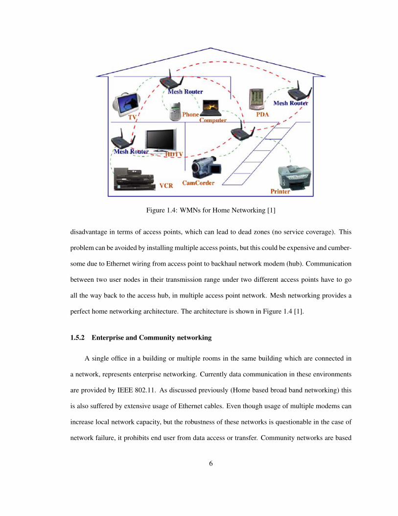
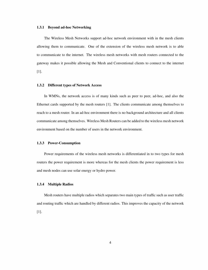
Figure 1.4: WMNs for Home Networking [1]

disadvantage in terms of access points, which can lead to dead zones (no service coverage). This

problem can be avoided by installing multiple access points, but this could be expensive and cumber-

some due to Ethernet wiring from access point to backhaul network modem (hub). Communication

between two user nodes in their transmission range under two different access points have to go

all the way back to the access hub, in multiple access point network. Mesh networking provides a

perfect home networking architecture. The architecture is shown in Figure 1.4 [1].

1.5.2 Enterprise and Community networking

A single office in a building or multiple rooms in the same building which are connected in

a network, represents enterprise networking. Currently data communication in these environments

are provided by IEEE 802.11. As discussed previously (Home based broad band networking) this

is also suffered by extensive usage of Ethernet cables. Even though usage of multiple modems can

increase local network capacity, but the robustness of these networks is questionable in the case of

network failure, it prohibits end user from data access or transfer. Community networks are based

6

on cable or DSL internet connection. Wireless routers, which are connected to internet modem are

being used by the end users for the internet access. This network is effective with for an individual

user, but this suffers from reduced network utilization, as all the information transfer should go

through internet with in a neighborhood. Wireless mesh networks (WMNs) can be very effective in

these scenarios, due to its flexible connections between offices and neighborhoods. Availability of

multiple paths to access internet despite of link failures can improve the network robustness.

1.5.3 Other Applications of Wireless Mesh Networks

Major advantages such as scalability and internal communication (with in the mesh clients)

have made Wireless Mesh Networks ideal for metropolitan area networking (MAN), transportation

systems, building automation, Health and Medical Systems. Mesh networks can also be imple-

mented in moving train, so that the passengers in a train can communicate among themselves and

access the internet through a gateway in the vehicle. WMNs can be useful tool in the surveillance

and health care institutions (patients data can be stored and accessed from different locations, so this

helps doctors in faster diagnosis and better services). The architecture for Transportation Systems

is shown in Figure 1.5. [1].

The Wireless Mesh Networks can also be used in various Electrical and power companies

to control the machines. In the present world the various systems in the industry are controlled

using the wired network. But the wired network is difficult to deploy and expensive, recently Wi-

Fi networks are employed but not successful due to the backend ethernet connection which results

in high cost of deployment. In these cases the wireless mesh routers can be deployed and the

information from them can be used to control the electrical machines and motors [1].

In Health and Medical systems, the data of the patient is need to processed in different rooms in

an hospital. Present day hospitals used wired connections to transmit data from one room to another

which prohibits access of the data to all rooms due to the cumbersomeness of wired networks [1]. In

7

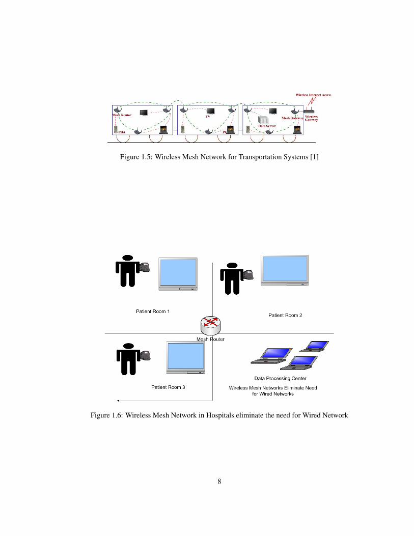
Figure 1.5: Wireless Mesh Network for Transportation Systems [1]

Figure 1.6: Wireless Mesh Network in Hospitals eliminate the need for Wired Network

8

wireless mesh networks as shown in the Figure 1.6 the data from different rooms can be transmitted

to the data processing center using mesh routers also the data can be transmitted globally bu using

the gateway connection to the internet.

Wireless Mesh Networks can also be used in security systems where the data can be transmitted

through the mesh routers. In wired networks the entire security area need to be covered using the

wired networks. But in wireless mesh networks when an emergency occurs in a new place simply

installation of one mesh router transfers the data through the entire emergency environment [1]. This

scenario has a vital importance during emergency disasters where the firefighters and the police can

deploy one wireless mesh router to transmit the data from an unknown emergency area without the

need of installing additional wired networks[1].

The rest of the document is organized as follows. Chapter 2 introduces the scalability problem

of wireless mesh networks and analyzes the variation of performance of wireless mesh networks

with respect to data rate of clients, error rate and gateway placement.Finally a solution to the scal-

ability problem is provided at the end of the chapter.Chapter 3 introduces the unfairness issue in a

multihop wireless mesh network environment. It deals with the different traffic models that demon-

strate unfairnes among different hops.The proposed GCA is presented in this chapter which provides

a solution for the unfairness issue in wireless mesh networks. Section 4 concludes this document.

9

CHAPTER 2

STUDY OF SCALABILITY IN WIRELESS MESH NETWORKS USING NS-2 SIMULATIONS

2.1 Definition of Scalability in Wireless Mesh Networks

In a telecommunication network environment it is desired that more and more number of nodes

are added to the network anytime without the degradation of the network performance. One of

the architecture advantages of wireless mesh networks is that the network can be scalable to any

number of nodes. But the existing protocols in wireless networks are not suited for the network to

be completely scalable. SO new protocols are to be designed or existing protocols must be modified

to support the scalability of wireless mesh networks.

In WMNs, it is desired that more nodes can be added when necessary. However, with the

existing 802.11 protocols as number of nodes increase, interference increases thereby decreasing

the throughput. It is shown that the asymptotic capacity for each node decreases with the number of

nodes as O(1/n) where n is the total number of nodes in the network [2]. The network performance

depends on a number of factors, the network performance varies with the error rate, data rate of

clients, gateway placement, propagating conditions and different carrier sensing thresholds. The

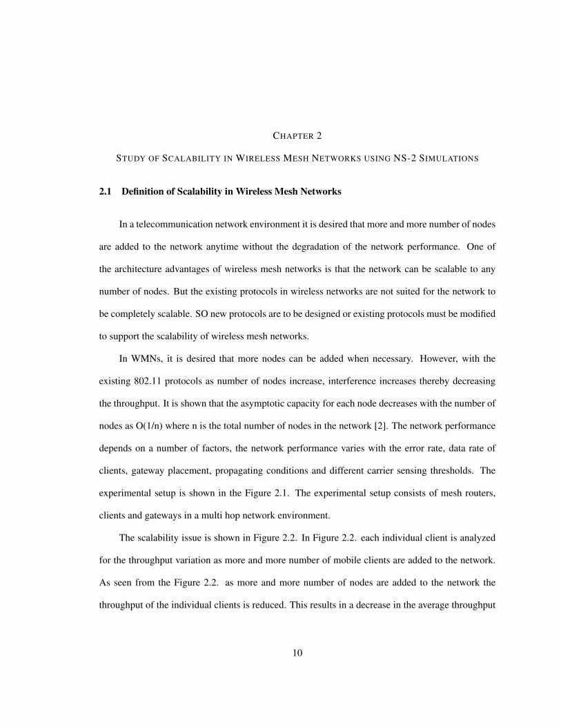
experimental setup is shown in the Figure 2.1. The experimental setup consists of mesh routers,

clients and gateways in a multi hop network environment.

The scalability issue is shown in Figure 2.2. In Figure 2.2. each individual client is analyzed

for the throughput variation as more and more number of mobile clients are added to the network.

As seen from the Figure 2.2. as more and more number of nodes are added to the network the

throughput of the individual clients is reduced. This results in a decrease in the average throughput

10

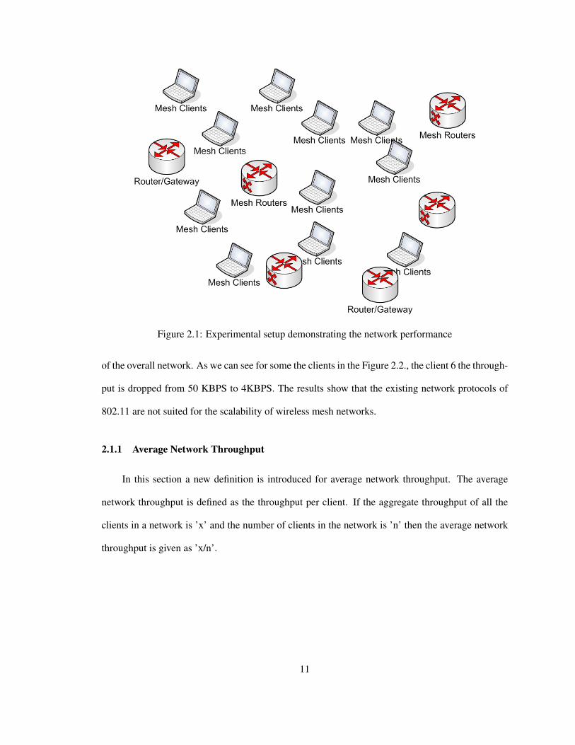
Figure 2.1: Experimental setup demonstrating the network performance

of the overall network. As we can see for some the clients in the Figure 2.2., the client 6 the through-

put is dropped from 50 KBPS to 4KBPS. The results show that the existing network protocols of

802.11 are not suited for the scalability of wireless mesh networks.

2.1.1 Average Network Throughput

In this section a new definition is introduced for average network throughput. The average

network throughput is defined as the throughput per client. If the aggregate throughput of all the

clients in a network is ’x’ and the number of clients in the network is ’n’ then the average network

throughput is given as ’x/n’.

11

Figure 2.2: Scalability in Wireless Mesh Networks

2.1.2 Characteristics of Average Network Throughput

There are a few characteristics for average network throughput such as it decreases with in-

crease in number of clients in the network, it depends on the data rate of the clients, error rate and

gateway placement.

The Lagrange polynomial [64] can be used to estimate the variation of the network perfor-

mance based on the number of clients. The Lagrange polynomial is an interpolating polynomial of

the nth order which passes through n+1 points and is given by

L(x)=∑n

j=0 yj(x)× lj(x) [64]

The Lagrange polynomial can be used to find the variation of overall network throughput. Here

we derive the Lagrange polynomial for 2 different cases. Let us derive the Lagrange polynomial for

2 different cases and observe the differences

Case 1:

12

In the case 1, let us consider a variation of mesh clients from 10 to 20. By Experimental results,

we have the network average throughput for 10 clients as 52.835Kbps. For 15 mesh clients we have

the network average throughput as 37.24Kbps, for 20 Mesh clients the network average throughput

is given as 22.03Kbps

x0 = 10.0 f(x0) = 52.835 x1 = 15.0 f(x0) = 37.24 x2 = 20.0 f(x0) = 22.03

The basis polynomials are

l0(x) = 1.0567x2 − 36.9845x + 317.01

l1(x) = −1.4896x2 + 44.688x− 297.92

l2(x) = 0.4406x2 − 11.015x + 66.09

The final Lagrange polynomial is given as

L(x) = 0.0077x2 − 3.3115x + 85.18

If we substitute x=10 in the above equation we get the network average throughput as 52.815Kbps

which is almost same as the experimental results. If we substitute x=20 we have network average

throughput as 22.03Kbps which is same as the experimental results. From the Lagrange equation

we can find the network average through for any number of mesh clients in between 10 and 20 in

this topology. Let us verify the next case where the mesh clients are varied from 10 to 70.

Case 2: In this case if we consider ’r’ mesh routers , ’g’ gateways and the number of mesh

clients is varied from 10 to 70. The experimental results give us the network average through-

put as 60.283Kbps when the number of mesh clients are 10, When the number of mesh clients

are improved to 45 the network average throughput is given as 37.802Kbps, when the number of

mesh clients are improved to 70 the average network throughput is given as 17.32Kbps. Based on

these three results we can derive a polynomial which will allow us to estimate the average network

throughput for clients numbering between 10 and 70

x0 = 10.0 f(x0) = 60.28 x1 = 45.0 f(x0) = 37.802 x2 = 70.0 f(x0) = 17.32

The basis polynomials are

13

l0(x) = 0.028x2 − 3.3x + 90.42

l1(x) = −0.0604x2 + 4.838x− 30.2416

l2(x) = 0.0115x2 − 0.635x + 5.196

The final Lagrange polynomial is given as

L(x) = −0.0209x2 + 0.903x + 65.3744

where x is the number of mesh clients and x varies in between 10 and 70. With the help of

the above equation we can find the average throughput of the network for any number of clients

between 10 and 70 for the above topology.

If we substitute x=10 in this Lagrange equation we get average network throughput as 72.33Kbps.

The average network throughput for 50 mesh clients is given by substituting ’x’=50 in the above

equation, we get the average network throughput as 58.27Kbps.

As seen from the Lagrange equation in this case the average network throughput derived from

Lagrange equation just gives an approximate value but not the exact value. This is due to the fact

involved as there are many number of mesh clients in the environment and we derived the equation

only with 3 experimental results. For better results the equation should be derived using more

number of experimental results. So we can say that as more number of mesh clients are involved in

the network we should use more number of experimental results to get accurate approximations.

2.2 Variation of Network Performance

In moving forward with the wireless mesh network variation with respect to different parame-

ters we would like to introduce the two most familiar problems of wireless networking the hidden

terminal and exposed terminal problems

14

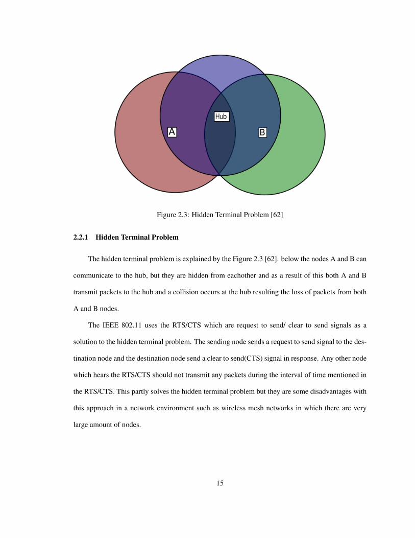
Figure 2.3: Hidden Terminal Problem [62]

2.2.1 Hidden Terminal Problem

The hidden terminal problem is explained by the Figure 2.3 [62]. below the nodes A and B can

communicate to the hub, but they are hidden from eachother and as a result of this both A and B

transmit packets to the hub and a collision occurs at the hub resulting the loss of packets from both

A and B nodes.

The IEEE 802.11 uses the RTS/CTS which are request to send/ clear to send signals as a

solution to the hidden terminal problem. The sending node sends a request to send signal to the des-

tination node and the destination node send a clear to send(CTS) signal in response. Any other node

which hears the RTS/CTS should not transmit any packets during the interval of time mentioned in

the RTS/CTS. This partly solves the hidden terminal problem but they are some disadvantages with

this approach in a network environment such as wireless mesh networks in which there are very

large amount of nodes.

15

Figure 2.4: Exposed terminal problem [63]

2.2.2 Exposed Terminal Problem

The exposed terminal problem is explained by referring to the Figure 2.4 [63]. below. When

the node S1 is sending data to R1, the node S2 cannot send data to R2. The hidden and exposed

terminal problems play an important part in determining the performance of wireless networks.

2.2.3 TCP Vs UDP

TCP and UDP are the transport layer protocols used for the transmission of the packets through

the internet. TCP is used for connection-oriented transmissions and UDP is used for connectionless

transmissions. In connection-oriented transmissions a connection is established between the end

users before transmission of any data, where as in the connectionless transmissions there is no

connection established between the end users. In general connection-oriented transmissions are

called reliable transmissions. TCP is a reliable protocol compared to the UDP.

In our simulation experiments TCP is used to transfer packets from the clients to the internet.

TCP has additional advantages compared to UDP such as error correction and flow control. Flow

control determines the flow of the packets from source to destination based on the window size

of the destination node. The TCP initiates a connection through threeway hand shake. When a

transmission is through TCP it is ensured that all the packets are received in the correct order to the

destination.

16

In modern days, Wired Networks the error rate is mainly negligible. TCP assumes that the

packet loss is due to the congestion in wired networks. But in the wireless networks the error

rates are not negligible, there are lot of other factors in wireless environment resulting in the packet

loss, but TCP which is designed for wired networks basically initiates the congestion algorithms

in wireless networks when there are loss of packets. Because of the congestion algorithms the

throughput of the wireless networks is greatly reduced as a result of decrease in the window size.

2.2.4 Error Rate vs Network Performance

It is obvious that with increase in the error rate the network performance decreases. Error rate

depends on various factors and it determines the number of successful packets in total number of

packets transmitted. The packet error rate depends on the bit error rate and the collision time. In the

simulation environment used the error rate is introduced so as to calculate the effect of error rate on

network performance. In the NS2 simulation environment the error model uses a flag on the packet

to introduce errors in the transmission. There is a error rate factor in the simulation environment

which allows us to change the error rate for different simulations. In our experiment we simulated

the network for 4 different error rates randomly. For a multi-hop wireless mesh environment, the

hop performance variation with respect to the error rate is shown in Figure 2.5. As depicted from the

figure the error rate for the network affects the 3rd hop clients. As the error rate increases the loss

of packets increases and the retransmissions are increased. Due to this, the packets from the farther

hops experience more hidden terminal and exponential back-off problems, resulting in a severe loss

of throughput. The results show that the 3rd hop performance is almost zero with an increase in the

error rate. The Experimental Results are depicted in Figure 2.5.

17

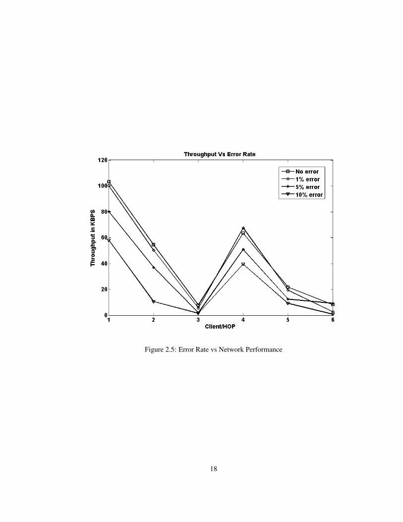
Figure 2.5: Error Rate vs Network Performance

18

2.2.5 Data Rate of Clients vs Network Performance

Different mesh clients transmit at a different data rate. Based on the applications accessed by

the clients the data rate required for the successful running of application varies. So the clients which

are accessing different applications have different data rates. The overall network performance is

affected by the data rate of the individual clients. The variation of the throughput of the clients with

respect to the data rate is observed. The simulation is performed using 100 mesh clients. In addition,

the percentage of high data rate clients is varied in different simulation scenarios. Examples of some

of the applications requiring high data rate are video streaming and some examples of low data rate

applications are text messaging. In the experimental setup the percentage of high date rate clients is

taken as the measure of variation, the percentage of high data rate clients is varied in three different

scenarios and the results are plotted comparing each other. The results are shown in Figure 2.6.

In the Figure 2.6. equally distributed clients refers that half of the clients are using low data rate

applications and another half of the clients are using high data rate applications. In the second

and third scenario the high data rate clients is improved to 75 percent and 85 percent respectively.

The high data rate clients transmit data at a faster rate and hence the interference increases and the

throughput decreases, which are depicted in the experimental results.

2.2.6 Gateway Placement vs Network Performance

Also the hop performance is affected by the placement of the gateways. The number of gate-

ways and the placement of the gateways can be changed in an environment. By experimenting with

different placement of the gateways, the maximum performance is determined. In an ’n’ mesh/

conventional client environment, there is a need for n/2 mesh routers and n/6 gateways and the

placement of the gateways is in such a way that the gateways always hold the center of the mesh

routers. The performance of the gateway arrangement compared to the distributed gateway is com-

pared. The results are shown in Figure 2.7. Comparing the results of the gateway placement, it

19

Figure 2.6: Data Rate vs Network Performance

shows that properly choosing the gateways will affect the performance of the overall throughput of

the network. The Results are shown in Figure 2.7.

2.2.7 Data Rate vs Number of Clients vs Network Performance

As the number of clients increases the interference increases and also as the data rate of the

clients increases the interference increases. In this case both are taken in to consideration.

The threshold throughput here is defined as the minimum average network throughput so that

each client can access the internet. If the Average network throughput is below the threshold one

or more of the network clients cannot access the internet. From the simulation results shown in the

above Figure 2.8. as the data rate of the clients is increased the threshold is reached early compared

to less data rate clients. In the above example for the datarate 1 the threshold is reached at 55 clients

that is all the 55 clients are able to access the internet. In the datarate 2 the threshold is reached for

20

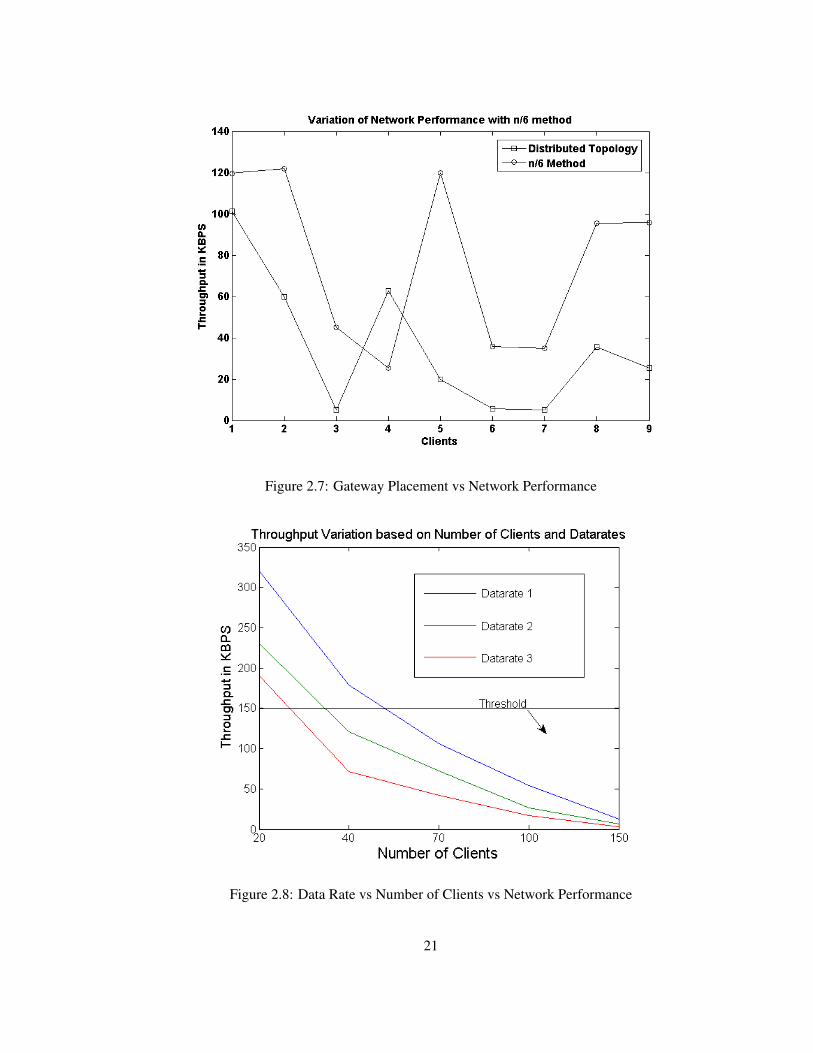
Figure 2.7: Gateway Placement vs Network Performance

Figure 2.8: Data Rate vs Number of Clients vs Network Performance

21

less number of clients 38 clients that is as the data rate is increased only 38 clients are able to access

the internet. In the data rate 3 only 28 clients are able to access the internet.

2.3 Reasons for Scalability and Fairness Issues

The main reason for the fairness/scalability problems is due to the contention of the channel by

the clients. The contention of the channel is affected by many factors such as the gateway placement,

error rate, traffic model, and the type of connection (TCP or UDP). TCP needs an acknowledgement

for every packet, whereas UDP does not need an acknowledgement for every packet. The focus is

mainly given on TCP connection in this article because as the TCP connection performance is

increased in any model, the UDP performance is obviously increased. By the above results, we can

see that network throughput or the unfairness in the hops depends on many factors, including data

rate of the clients, placement of the routers/gateways, and error rate. Also, the throughput of the

clients depends on different aspects such as traffic model used and type of connection used. The

network must be scalable with the addition of clients but as the interference increases so the network

overall throughput decreases.

2.4 Differentiated Clients Algorithm to Improve Scalability

2.4.1 Algorithm for scalability

The algorithm described here is completely dynamic as more and more nodes are added to the

network at any instant of time so as to make the network scalable.It is evident that the throughput

in a wireless network is related to interference and transmission time. As the nodes are added

to the existing wireless mesh network the interference increases among the nodes. Therefore as

the number of nodes increase the throughput decreases. In this section we focus on improving

the throughput by reducing the interference. In order to increase throughput (capacity), we need

to decrease the interference by some ways. We got an idea from the sleeping node in SMAC,

22

which is for energy saving while waiting for wake-up. Our approach to decrease interference is

implemented by stopping transmission of an application and buffering for some time. It seems to

be similar to sleeping node, but different. Controlling of nodes is done in a periodic way so that

no nodes are affected in a negative way. There are many types of applications and we classified

them in to two types: high data rate applications and low data rate applications. Of course the

high data rate applications demand more capacity of the channel than low data rate ones. So we

use the low data rate applications to reduce the interference and increase the overall throughput of

network. Firstly, applications with lesser data transfer rate are identified. The less data transfer rate

applications are text messaging, browsing etc and high data rate applications are video streaming,

online TV, download of huge files etc. Secondly, transmitting nodes with lesser data rate transfer are

momentarily stopped and data is maintained in output buffer. The nodes are controlled in a periodic

way so that each low data rate node is affected in the algorithm once or twice so that its performance

is not deteriorated. The algorithm is completely dynamic and the low data rate nodes are controlled

based on different factors such as the number of clients in the network, average network throughput

and the number of transmitting nodes in the vicinity of the low data rate clients.

We used the network simulator ns2 tool for implementing our idea. The topology is given

below. We simulated a base total of 100 802.11 nodes of which 64 are mesh clients and remaining

act as mesh routers. Some of the mesh routers act as gateways through which the traffic flows to

and from the internet. In the network region the gateway mesh routers are considered to be the final

destinations. The gateways are connected to the internet by using wired connections. The wired

connections from the gateways to the internet support huge data rates and very less error rates. The

mesh routers that act as the gateways are chosen at a proper locations in the environment so that

the clients are not too far away from the gateways. The gateways are to be chosen so that as more

and more nodes are added to the network environment the clients are still able to access the internet

regardless of the interference problems. In our experiment among the 64 mesh clients 32 clients

23

Figure 2.9: Experimental setup for Scalability Issue

are chosen as high data rate applications and 32 are chosen as low data rate applications. More and

more nodes are added on and off in general case so as to make the network scalable. In general

the different clients transfer at a different data rate based on the needs of the user. The clients are

distributed uniformly in the entire network environment regardless of the high data rate or low data

rate. The experimental setup is as shown below in Figure 2.9.

The simulation procedure is as follows: N Clients N/2 high data rate and N/2 low data rate

Step1: All N active clients Step2: 3N/4 active clients (N/4 low data rate active) Step3: N/2 active

clients (N/2 low data rate inactive)

The above procedure is explained as follows in the step1 all the clients are active that is there

is no algorithm implemented in the step1. In general the network performance is determined based

on the actual environment. In this case all the 64 mesh clients are active, none of the low data rate

mesh clients are controlled.

24

In the step2 N/4 low data rate clients are controlled based on the vicinity of the client, average

network throughput and the number of high data rate clients that are actually transmitting data. In

this case 8 low data rate clients are controlled in a period way out of the 32 low data rate clients.

The 8 low data rate clients are controlled in such a way that none of the performance is deteriorated.

The application is buffered and made sure the packet reaches before the end of the timer in a TCP

connection.

In the Step3 N/2 low data rate clients are controlled based on the algorithm procedure so as to

improve the performance of the overall network. In this case 16 low data rate clients are controlled.

In the above cases more and more nodes are added to the network environment at any instant

making the network scalable. The number ’N’ is varied in real world environment from time to

time.

We compared the throughput in the three cases and we got the results as follows. We ana-

lyzed our idea for mobile nodes and stationary nodes. The simulation results are as shown in the

Figure 2.10.

As seen in the experimental results the throughput of different clients is varied in all the above 3

steps. In this case the overall average network throughput is also increased in the 3 steps.The overall

average network throughput variation in all the above three steps is as shown in the figure 2.11.

25

Figure 2.10: Performance of scalability algorithm

Figure 2.11: Performance of scalability algorithm Overall Average Network Throughput

26

CHAPTER 3

STUDY FAIRNESS IN WIRELESS MESH NETWORKS USING NS-2 SIMULATIONS

3.1 Definition of Fairness in Wireless Mesh Networks

In wireless mesh networks the nodes farther away from the gateway may be starved by nodes

closer to the gateway[3]. This is due to the fact that the clients that are farther hops away exhibit

frequent exponential back off. This leads to a higher probability of collision and loss, and a corre-

sponding throughput decrease. This leads to unfairness among different clients in different hops in

sharing of the throughput of the channel.

3.2 Related Work in Fairness Issue

There are various methods proposed to modify the back-off algorithm and contention windows

for improving fairness which can be found in [59] [61]. One more approach NAV-blocking in

which each Access Point transfers a beacon which does not allow the mobile stations to transmit

during that interval [7]. The Forced Handoff technique forces the mobile stations between different

Base Stations to switch between different base stations to achieve a fair throughput [7]. We used a

Gateway Classification Algorithm in which the gateways are differentiated to handle different types

of traffic.

3.3 Analysis of the Fairness Issue

In cellular networks, the network area is divided in to cells and each mobile user is only one hop

away from its base station [11]. The other mobile users need not transmit the traffic of other mobile

27

Figure 3.1: Idle vs Practical Fairness [2]

users to the base station. But in a wireless mesh network environment a mobile client user node

has to transmit relayed traffic and also its own traffic. In a wireless mesh network the mesh clients

contend among one another for the destination node or mesh router which transmits the traffic to

the gateway and also between its traffic and the relayed traffic [2]. The contention environment is

different in wireless LANs in infrastructure mode and cellular networks because the user nodes are

only at one-hop distance from the access point and base station respectively[2].

The fairness problem is clearly explained by the Figure 3.1[2] there are two nodes,node 1 and

node 2 which are offered a load of G. The destination node for the two nodes is the gateway node

(GW) as shown in the figure. In the ideal case the channel is shared equally among the 2 nodes as

the offered load (G) increases as shown in the Figure 3.1. But in practical case as the mesh clients

have to contend between the relay traffic and its own traffic the node that is closer to the gateway

node 1starves the node far away from the gateway The result in Figure 3.1 is obtained under the

fact that the traffic to be forwarded by node 1 originating from the node 2 is queued together with

the traffic from its own node 1[2]. So the correlation between different mesh clients fail to provide

end-to-end fairness in multihop wireless mesh networks.

In a Wireless Mesh Network, there are several gateways. The gateways along with the mesh

routers form a multi-hop environment for the mesh and conventional clients. We consider the topol-

ogy as shown in the following Figure 3.2.

28

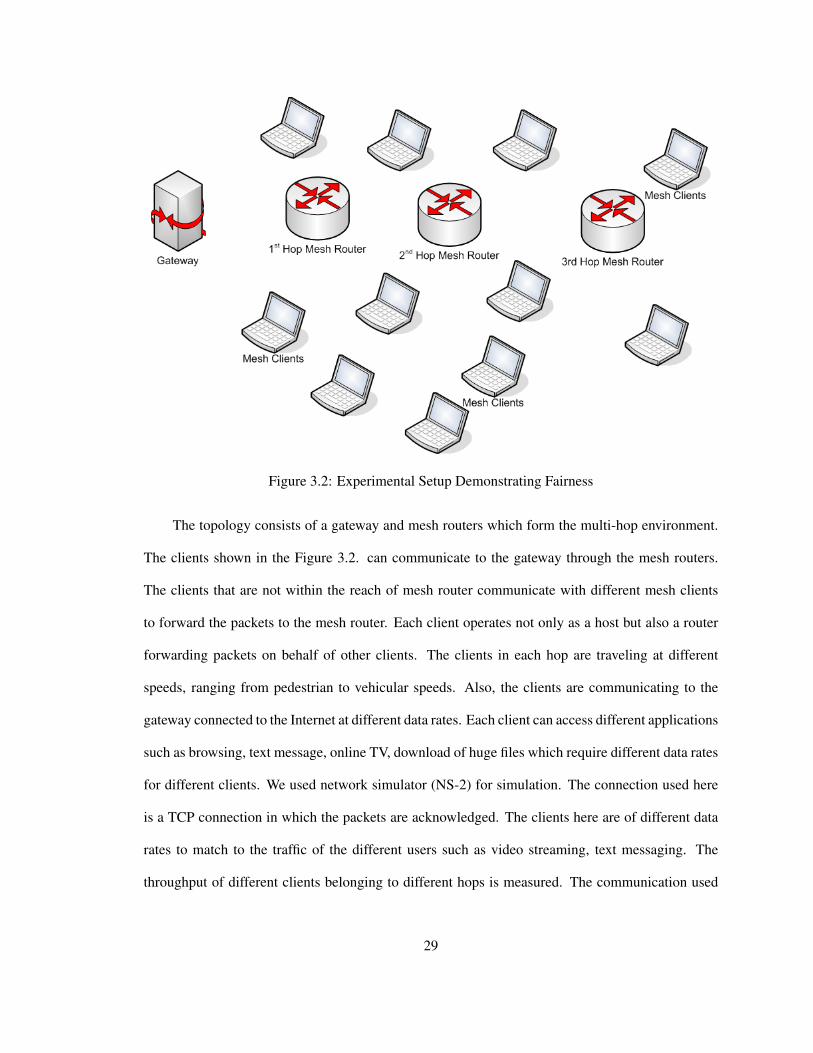
Figure 3.2: Experimental Setup Demonstrating Fairness

The topology consists of a gateway and mesh routers which form the multi-hop environment.

The clients shown in the Figure 3.2. can communicate to the gateway through the mesh routers.

The clients that are not within the reach of mesh router communicate with different mesh clients

to forward the packets to the mesh router. Each client operates not only as a host but also a router

forwarding packets on behalf of other clients. The clients in each hop are traveling at different

speeds, ranging from pedestrian to vehicular speeds. Also, the clients are communicating to the

gateway connected to the Internet at different data rates. Each client can access different applications

such as browsing, text message, online TV, download of huge files which require different data rates

for different clients. We used network simulator (NS-2) for simulation. The connection used here

is a TCP connection in which the packets are acknowledged. The clients here are of different data

rates to match to the traffic of the different users such as video streaming, text messaging. The

throughput of different clients belonging to different hops is measured. The communication used

29

Figure 3.3: Unfairness Issue

here is a TCP communication which requires all the packets to be acknowledged back to the client.

The transmission time for each successful packet is the total time in between release of the packet

from the client and the time in which the acknowledgement is received. The throughput variation

of the different hop clients is shown in Figure 3.3.

The Figure 3.3. shows that the throughput varies among different hops. The farther away hops

experience frequent exponential back-off than the nearby hops as stated in [3]. The farther away

hops from the gateway are starved due to the near hops from the gateway. The throughput variation

of the first and the third hops differs a lot as shown in the Figure 3.3.

As the data rate of clients increases the far away hops are starved. If the data rate of the clients

is very less than the clients up to 5th or 6th hops can access the gateway. The Lagrange polynomial

30

Figure 3.4: Throughput of Different Clients

as described in chapter 2 can also be used here to find the equation of the hop throughput for general

nth hop.

A simulation environment with 100 mesh clients traveling at different speeds and 30 mesh

routers in which three routers (10 percent of the total routers) act as gateways are randomly deployed

and the performance of the clients is measured. It is observed that different clients have different

throughputs which demonstrates the unfairness issue. As seen from the Figure 3.4. eventhough

all the clients are in the same network area they are not able to share the resources fairly. The

throughput varies depending on the hop of the client as illustrated in Figure 3.4.

31

3.4 Unfairness in Different Traffic Models

3.4.1 Different Traffic Models

There are different types of traffic models used in the real network environment such as Expo-

nential, Pareto and CBR.

The Exponential ON/OFF traffic generator in a simulation environment has different parame-

ters such as packetsize,bursttime, idletime and rate. The burst time is the average ’on’ time for the

traffic generator, the idle time is the average ’off’ time for the generator and rate is the sending rate

of the packets during the ’on’ time [48].

In ns-2 simulation environment the Exponential On/Off generator can be made to work as a

Poisson generator by changing the variable bursttime to 0 and by changing the variable rate to a

very large value. The C++ code ensures that even if the burst time is set to zero, at least one packet

is sent [48]. And also the next interarrival time is the sum of the assumed packet transmission time

and the random variate corresponding to idle time[48]. To make the first term in the sum very small,

make the burst rate very large so that the transmission time is almost zero compared to the typical

idle times [48].

The CBR traffic generator has different parameters such as packetsize, rate and random. The

rate is the constant rate at which the packets are sent, random is the flag indicating whether or not

to introduce random “noise” in the scheduled departure times [48].

The fairness issue is demonstrated for different types of user traffic models. The exponential

and CBR traffic models are used as the user traffic. The following results show the Unfairness for

different traffic models. In the first case Figure 3.5 all the clients use Exponential traffic and in the

second case Figure 3.6 all the clients use CBR traffic. As seen from the results both the exponential

and CBR traffic models have unfairness issue in the hops. If there is some factor to control the

32

Figure 3.5: Variation of Hop Performance for Exponential Traffic

network traffic, we could have avoided the fairness to some extent. There is no factor as to control

the unfairness in these type of traffic models.

Earlier in this section we performed the experiment on Exponential and CBR traffic models.

Now we have focused our attention on the Pareto Traffic Model which allow us to modify some

factors to improve the fairness of the far way hops. The Pareto On/Off Traffic Generator is a traffic

generator embodied in the OTcl class Application/Traffic/Pareto. It generates traffic according to

a Pareto On/Off distribution. Packets are sent at a fixed rate during on periods, and no packets

are sent during off periods. Both on and off periods are taken from a Pareto distribution with

constant size packets. These sources can be used to generate aggregate traffic that exhibits long

range dependency. There are various input parameters in the pareto traffic model such as burst time,

33

Figure 3.6: Variation of Hop Performance for CBR Traffic

34

idle time, rate, packet size and shape. In each On/Off round the next burst time and next idle time are

computed based on the pareto shape parameter. The next burst time refers to the number of packets

to be transmitted in the next burst period. Based on the characteristics of the pareto traffic model

the numbers of packets send during the on-time of an application can be varied.In a Wireless Mesh

Network as we know the farther away hops are starved by the hops closer to the gateway. Using

the characteristics of pareto traffic model the farther away hops are made to send more number of

packets during the on period than the hops that are closer to the gateway by varying the pareto shape

parameter. This improves the performance of the far away hops as compared to without using this

algorithm. Now here the Pareto shape parameters are setup in such a way that the clients that are

father hops away from a gateway are made to send more number of packets during the on time as

compared to the clients that are nearer to the gateway. This algorithm is applied to observe the

improvement in the performance of the far away hops. The experimental results are as shown in

Figure 3.7.

3.5 Gateway Classification Algorithm (GCA)

In Chapter 2 the network performance is observed by properly placing the gateways in a net-

work environment, the gateways are not classified into different types. The results are obtained by

changing the position of the gateways. In the results, we can observe a change in the throughput

of the overall network. This gave us an idea that the gateways can be modified in order to vary the

network performance. In this section, we classify the gateways into different types. In a wireless

mesh networks, there are several gateways. We classify the gateways into two types: high data rate

gateways and low data rate gateways. The high data rate gateways are responsible for handling the

traffic of the high data rate clients. The low data rate gateways are responsible for handling the low

data rate clients. By classifying the gateways into these two types, we can improve the performance

in terms of fairness. The traffic from the clients is routed to the appropraite gateway based on the

35

Figure 3.7: Improvement in Hop Performance using Pareto Traffic Model

36

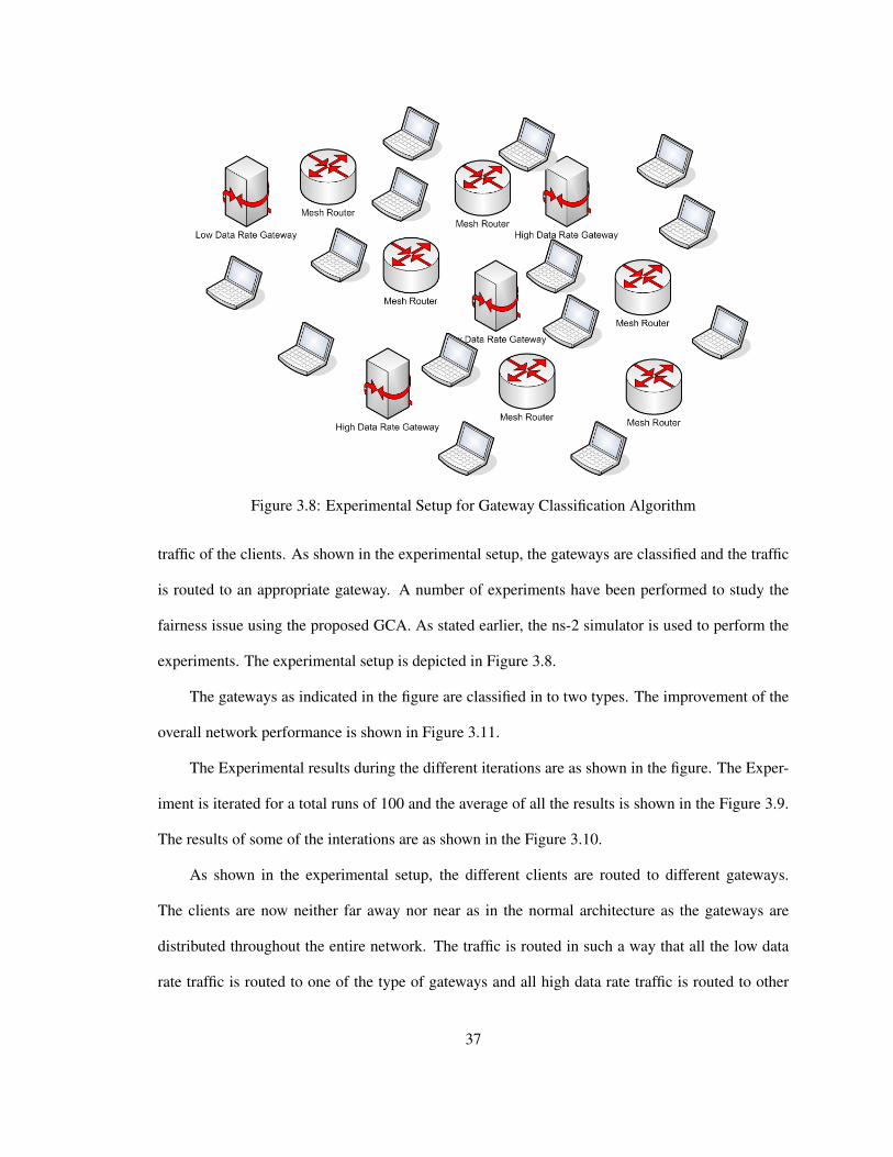
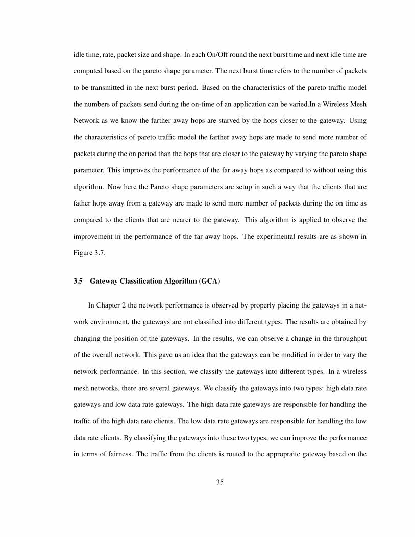
Figure 3.8: Experimental Setup for Gateway Classification Algorithm

traffic of the clients. As shown in the experimental setup, the gateways are classified and the traffic

is routed to an appropriate gateway. A number of experiments have been performed to study the

fairness issue using the proposed GCA. As stated earlier, the ns-2 simulator is used to perform the

experiments. The experimental setup is depicted in Figure 3.8.

The gateways as indicated in the figure are classified in to two types. The improvement of the

overall network performance is shown in Figure 3.11.

The Experimental results during the different iterations are as shown in the figure. The Exper-

iment is iterated for a total runs of 100 and the average of all the results is shown in the Figure 3.9.

The results of some of the interations are as shown in the Figure 3.10.

As shown in the experimental setup, the different clients are routed to different gateways.

The clients are now neither far away nor near as in the normal architecture as the gateways are

distributed throughout the entire network. The traffic is routed in such a way that all the low data

rate traffic is routed to one of the type of gateways and all high data rate traffic is routed to other

37

Figure 3.9: Results of Iterations without Using Gateway Classification Algorithm

38

Figure 3.10: Results of Iterations with Using Gateway Classification Algorithm

39

Figure 3.11: Throughput Variation Using Gateway Classification Algorithm

type of gateways. The clients do not experience the exponential back-off frequently as in the normal

architecture. Because of this, the throughput of the overall network is distributed in a reasonable

manner. As depicted in the Figure 3.12., the variation of the throughput of the clients in the two

different cases and the overall performance distributed in a fair manner. The variation of throughput

of different clients is shown in Figure 3.12.

In the above Figure 3.12. the variation of throughput of each individual client is observed after

the implementation of the algorithm. It can be obviously seen that the performance of each client is

improved based on the gateway classification algorithm.

The histogram in Figure 3.13. shows the number of clients at different throughput ranges.

We can observe the increase in the number of clients in the range of 2nd hop throughput. As

shown in the Figure 3.13., the throughput variation is huge. Without GCA the number of clients

in the throughput range (0-10) are 83. After the application of the proposed GCA, the number of

40

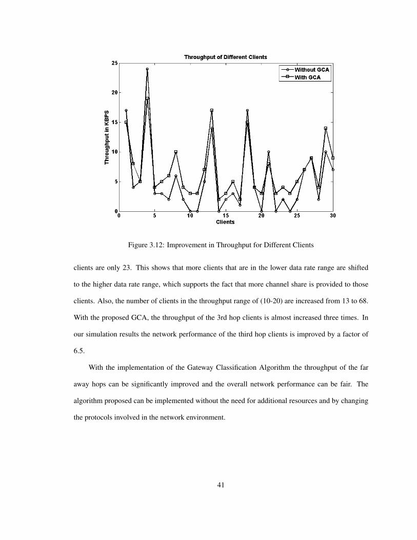
Figure 3.12: Improvement in Throughput for Different Clients

clients are only 23. This shows that more clients that are in the lower data rate range are shifted

to the higher data rate range, which supports the fact that more channel share is provided to those

clients. Also, the number of clients in the throughput range of (10-20) are increased from 13 to 68.

With the proposed GCA, the throughput of the 3rd hop clients is almost increased three times. In

our simulation results the network performance of the third hop clients is improved by a factor of

6.5.

With the implementation of the Gateway Classification Algorithm the throughput of the far

away hops can be significantly improved and the overall network performance can be fair. The

algorithm proposed can be implemented without the need for additional resources and by changing

the protocols involved in the network environment.

41

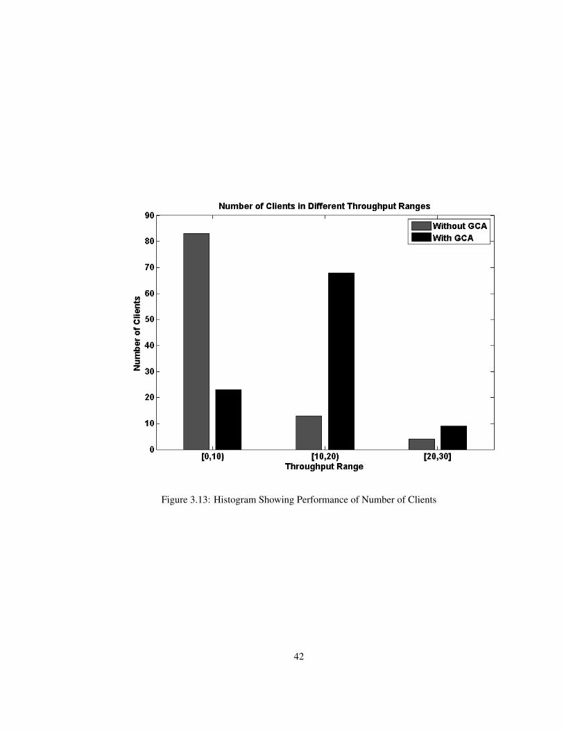
Figure 3.13: Histogram Showing Performance of Number of Clients

42

CHAPTER 4

CONCLUSION

Wireless mesh networks have many advantages, and also there are other issues which need

more investigation. Other issues associated with the mesh networks are scalability, mobility, unfair-

ness and security. More investigation is needed in these areas. In the first chapter of this thesis, we

presented the characteristics, applications and problems associated with wireless mesh networks.

In the second chapter we analyzed the variation of the performance of wireless mesh networks

with respect to different parameters such as error rate, gateway placement, data rate of clients. In

this chapter we also demonstrated the scalability issue and proposed a differentiated clients algo-

rithm to solve the scalability problem. The algorithm proposed is a dynamic algorithm and the

performance improves as more and more mesh clients are added to the network environment. The

algorithm is verified using the NS-2 simulation environment and the results obtained show a signif-

icant improvement in the performance.

In the third chapter the unfairness in multi-hop wireless mesh networks is introduced and the

performance of different traffic models such as the exponential, Constant Bit Rate and the Pareto

traffic models on different hops is observed. Finally a Gateway classification algorithm is proposed

which differentiates the gateways in the environment and the traffic is routed to the appropriate

gateway. The simulation is performed using ns-2 simulator and the results obtained show a signifi-

cant improvement in the performance of the far way hop clients. In the future the improvement in

throughput performance when both, differentiated client and differentiated gateway algorithms are

employed will be studied and heterogenous clients will be deployed to emulate realistic scenarios.

43

BIBLIOGRAPHY

[1] I.F. Akyildiz and X. Wang, “A Survey on Wireless Mesh Networks,” IEEE CommunicationsMagazine, September 2005.

[2] J. Jun, “The nominal capacity of wireless mesh networks,” Wireless Communications, IEEEVolume 10, Issue 5, September 2005.

[3] V. Gambiroza, B. Sadeghi and E. Knightly, “End-to-End Performance and Fairness in Multi-hop Wireless Backhaul Networks,” Proceedings of ACM MobiCom 2004, Philadelphia, PA,September 2004.

[4] C.W. Hsu, C.Y. Wang and T.C. Hou, “Providing End-to-End Fairness in Wireless Mesh Net-works with Chain Topologies,” Parallel and Distributed Computing and Systems, November2006.

[5] N. Bisnik, and A. Abouzeid, “Delay and throughput in random access wireless mesh net-works,” Proceedings of IEEE International Conference on Communications ICC’06, June2006.

[6] D. Zhao, “Inter-AP coordination for fair throughput in infrastructure-based IEEE 802.11 meshnetworks,” International Conference on Wireless Communications and Mobile Communica-tions, Vancouver, Canada, July 2006.

[7] D. Zhao, “Achieving fair throughput in infrastructure-based IEEE 802.11 mesh networks,”IEEE GLOBECOM’06, December 2006.

[8] R.G. Cheng, C.Y. Wang and L.H. Liao, “Ripple: A Distributed Medium Access Protocol forMulti-hop Wireless Mesh Networks,” Vehicular Technology Conference, September 2006.

[9] B. Braunstein, T. Trimble, R. Mishra, B.S. Manoj and R. Rao, “On The Traffic Behaviorof Distributed Wireless Mesh Networks,” International Symposium on a World of Wireless,Mobile and Multimedia Networks, June 2006.

[10] R. Cheng, C. Wang, L. Liao, and J. Yang, “Ripple: A wireless token-passing protocol formulti-hop wireless mesh networks,” Communications Letters, IEEE, September 2006.

[11] N.B. Salem and J.P. Hubaux, “Securing wireless mesh networks,” Communications Letters,IEEE, September 2006.

[12] B. Aoun, R. Boutaba and G. Kenward, “Analysis of Capacity Improvements in Multi-RadioWireless Mesh Networks,” Vehicular Technology Conference, September 2006.

44

[13] R.K. Lam, D. Chiu and C.S. Lui, “On the Access Pricing Issues of Wireless Mesh Networks,”International Conference on Distributed Computing Systems, July 2006.

[14] T. Wu, Y. Xue and Y. Cui, “Preserving Traffic Privacy in Wireless Mesh Networks,” Interna-tional Symposium on a World of Wireless, Mobile and Multimedia Networks, June 2006.

[15] A. Acharya, A. Misra and S. Bansal, “Design and analysis of a cooperative medium accessscheme for wireless mesh networks,” First International Conference on Broadband Networks,2004.

[16] R. Luo, D. Belis, R.M. Edwards and G.A. Manson, “simulation design for link connection-oriented wireless mesh networks,” 4th International Workshop on Mobile and Wireless Com-munications Network, 2002.

[17] P. Beckman, S. Verma and R. Rao, “Use of mobile mesh networks for inter-vehicular commu-nication,” Vehicular Technology Conference, 2003.

[18] A. Raniwala and T. Chiueh, “Evaluation of a wireless enterprise backbone network architec-ture,” 12th Annual IEEE Symposium on High Performance Interconnects, 2004.

[19] S. Naghian, “Mesh vs. point-to-multipoint topology: a coverage and spectrum efficiency com-parison,” 15th IEEE International Symposium on Personal, Indoor and Mobile Radio Com-munications, 2004.

[20] L. Iannone, R. Khalili, K. Salamatian and S. Fdida,“Cross-layer routing in wireless meshnetworks,” International Symposium on Wireless Communication Systems, 2004.

[21] A. Adya, P. Bahl, J. Padhye, A. Wolman, L. Zhou, “A multi-radio unification protocol for IEEE802.11 wireless networks,” First International Conference on Broadband Networks, 2004.

[22] F. Tasaki, H. Tamurat, M. Sengokut and S. Shinodas, “A new channel assignment strategytowards the wireless mesh networks,” 5th International Symposium on Multi-DimensionalMobile Communications Proceedings, 2004.

[23] P.H. Hsiao and H.T. Kung, “Layout design for multiple collocated wireless mesh networks,”Vehicular Technology Conference, 2004.

[24] M.K. Marina and S.R. Das, “A topology control approach for utilizing multiple channels inmulti-radio wireless mesh networks,” 2nd International Conference on Broadband Networks,2005.

[25] V. Navda, A. Kashyap and S.R. Das, “Design and evaluation of iMesh: an infrastructure-modewireless mesh network,” IEEE International Symposium on a World of Wireless Mobile andMultimedia Networks, 2005.

[26] A.K. Das, H.M. K. Alazemi, R. Vijayakumar and S. Roy, “Optimization models for fixed chan-nel assignment in wireless mesh networks with multiple radios,” 2005 Second Annual IEEECommunications Society Conference on Sensor and Ad Hoc Communications and Networks,2005.

45

[27] B. Ji, “Asynchronous wireless collision detection with acknowledgement for wireless meshnetworks,” Vehicular Technology Conference, 2005.

[28] L. Liu and G. Feng, “Research on Multi-constrained QoS Routing Scheme Using Mean FieldAnnealing,” Sixth International Conference on Parallel and Distributed Computing, Applica-tions and Technologies, 2005.

[29] C. Zhu, M.J. Lee and T. Saadawi, “On the route discovery latency of wireless mesh networks,”Consumer Communications and Networking Conference, 2005.

[30] K. Balaji, N. Hegde, B. Venkata Ramana, B. S. Manoj, and C. Siva Ram Murthy,“Performanceevaluation of a hybrid wireless network architecture for rural communication,” IEEE Interna-tional Conference on Personal Wireless Communications, 2005.

[31] F.H.P. Fitzek, T.K. Madsen, R. Prasad and M. Katz, “Cooperative IP header compression forparallel channels in wireless meshed networks,” IEEE International Conference on Communi-cations, 2005.

[32] P.M. Ruiz and A.F. G. Skarmeta, “Approximating optimal multicast trees in wireless multihopnetworks,” IEEE Symposium on Computers and Communications, 2005.

[33] R. Liscano, E.F. Sadok and E.M. Petriu , “Mobile wireless RSA overlay network as criticalinfrastructure for national security,” IEEE International Workshop on Measurement Systemsfor Homeland Security, Contraband Detection and Personal Safety Workshop, 2005.

[34] I.F. Akyildiz, “Key technologies for wireless networking in the next decade,” InternationalConference on Pervasive Services, 2005.

[35] L. Fu, Z. Cao and P. Fan, “Spatial reuse in IEEE 802.16 based wireless mesh networks,” IEEEInternational Symposium on Communications and Information Technology, 2005.

[36] S. Thuel and R. Cruz, “The next big bang in wireless and mobile communication,” 14th Inter-national Conference on Computer Communications and Networks, 2005.

[37] K.N. Ting, Y.F. Ko and M.L. Sim, “Voice performance study on single radio multi-hop IEEE802.11b systems with chain topology,” 13th IEEE International Conference on Networksjointly held with IEEE 7th Malaysia International Conference on Communication, 2005.

[38] C.E. Seo, E.J. Leonardo, P. Cardieri, M.D. Yacoub, D.M. Gallego and A.A.M. de Medeiros,“Performance of IEEE 802.11 in wireless mesh networks,” International Conference on Mi-crowave and Optoelectronics,2005.

[39] W. Allen, A. Martin, A. Rangarajan, “Designing and deploying a rural ad-hoc communitymesh network testbed,” The IEEE Conference on Local Computer Networks, 2005.

[40] Y. Ma, “Improving wireless link delivery ratio classification with packet SNR,” InternationalConference on Electro information Technology, 2005.

[41] G. Goth, “Groups hope to avoid mesh standard mess,” Distributed Systems online, IEEE 2005.

46

[42] B. Cheng, S. Kalyanaraman and M. Klein, “A geography-aware scalable community wirelessnetwork test bed,” First International Conference on Testbeds and Research Infrastructures forthe Development of Networks and Communities, 2005.

[43] I. Aydin, C. Jaikaeo, and C. Shen ,“Quorum-based match-making services for wireless meshnetworks,” IEEE International Conference on Wireless and Mobile Computing, Networkingand Communications, 2005.

[44] J.A. Stine, “Exploiting smart antennas in wireless mesh networks using contention access,”Wireless Communications, IEEE, 2006.

[45] C. Ma, Z. Zhang and Y Yang, “Battery-aware router scheduling in wireless mesh networks,”20th International Parallel and Distributed Processing Symposium, 2006.

[46] Jane- Hwa. Huang, Li-Chun. Wang and Chung-Ju. Chang, “Coverage and capacity of a wire-less mesh network,” International Conference on Wireless Networks, Communications andMobile Computing, 2005.

[47] T. Tsai and J. Chen, “IEEE 802.11 MAC protocol over wireless mesh networks: problemsand perspectives,” 19th International Conference on Advanced Information Networking andApplications, 2005.

[48] NS-2 manual documentation, “http://www.isi.edu/nsnam/ns/doc/index.html”.

[49] M. Kodialam and T. Nandagopal, “Characterizing Achievable Rates in Multi-Hop WirelessMesh Networks With Orthogonal Channels,” Transactions on Networking, IEEE, 2005.

[50] X. Tao, T. Kunz and D. Falconer,“Traffic balancing in wireless MESH networks,” InternationalConference on Wireless Networks, Communications and Mobile Computing, 2005.

[51] L. Liu and G. Feng, “Mean field network based QoS routing scheme in wireless mesh net-works,” International Conference on Wireless Communications, Networking and Mobile Com-puting, 2005.

[52] Z. Lei, Y. ShouBao, S. Weifeng and W. DaPeng, “Markov-Based Analytical Model for TCPUnfairness over Wireless Mesh Networks,” First International Multi-Symposiums on Com-puter and Computational Sciences, 2006.

[53] B. Wehbi, W. Mallouli and A. Cavalli, “Light Client Management Protocol for Wireless MeshNetworks,” International Conference on Mobile Data Management, 2006.

[54] H. Viswanathan and S. Mukherjee, “Throughput-range tradeoff of wireless mesh backhaulnetworks,” IEEE Journal on Selected areas in Communications, 2006.

[55] N. Funabiki, S. Yoshida, S. Tajima and T. Higashino, “An Internet Gateway Access-PointSelection Problem for Wireless Infrastructure Mesh Networks,” 7th International Conferenceon Mobile Data Management, 2006.

[56] D.M. Shrestha and Y.B. Ko, “On Construction of the Virtual backbone in Wireless Mesh Net-works,” The 8th International Conference Advanced Communication Technology, 2006.

47

[57] M.J. Lee, J. Zheng, Y.B. Ko and D.M. Shrestha, “Emerging standards for wireless mesh tech-nology,” Wireless Communications, IEEE, 2006.

[58] T. Tsai, H. Tseng and A. Pang, “A new MAC protocol for Wi-Fi mesh networks,” 20th Inter-national Conference on Advanced Information Networking and Applications, 2006.

[59] R.E. Ludwig, “Eliminating inefficient cross-layer interactions in wireless networking,” Ph.D.dissertation, Aachen University of Technology, Germany, 2000.

[60] V. Bharghavan, A. Demers, S. Shenker, and L. Zhang, “MACAW: a media access protocol forwireless LANs, in Proc. of ACM SIGCOMM94, 1994.

[61] J. Liu and S. Singh, “ATCP:TCP for mobile ad hoc networks,” IEEE Journal on selected areasin communications, vol. 19, no. 7,pp, 1300-1315, July 2001.

[62] www.wikipedia.com, “http://upload.wikimedia.org/wikipedia/en/thumb/b/b1/Hidden-node.svg/524px-Hidden-node.svg.png”.

[63] www.wikipedia.com, “Exposed Terminal Problem”.

[64] A. Quarteroni, R. Sacco, and F. Saleri, “Numerical Mathematics (Texts in Applied Mathemat-ics) (Hardcover)”, November, 2006.

48