Hardware Consolidation of Systolic Algorithms on a … · Hardware Consolidation of Systolic...
106
Hardware Consolidation of Systolic Algorithms on a Coarse Grained Runtime Reconfigurable Architecture A Thesis Submitted for the Degree of Master of Science (Engineering) in the Faculty of Engineering by Prasenjit Biswas Supercomputer Education and Research Centre INDIAN INSTITUTE OF SCIENCE BANGALORE – 560 012, INDIA JULY 2011
Transcript of Hardware Consolidation of Systolic Algorithms on a … · Hardware Consolidation of Systolic...
Hardware Consolidation of Systolic Algorithms on a
Coarse Grained Runtime Reconfigurable Architecture
A Thesis
Submitted for the Degree of
Master of Science (Engineering)
in the Faculty of Engineering
by
Prasenjit Biswas
Supercomputer Education and Research Centre
INDIAN INSTITUTE OF SCIENCE
BANGALORE – 560 012, INDIA
JULY 2011

To
The Flames of Life ....
Maa, Baba and Bon
“Keep your dreams alive. Understand to achieve anything requires faith
and belief in yourself, vision, hard work, determination, and dedication.
Remember all things are possible for those who believe.”
--- Gail Devers
Acknowledgments
First of all I would like to extend my sincere gratitude and respect to my supervisor Prof.
S. K. Nandy for his constant guidance and support during the entire curriculum of my
M.Sc(Engg.) program. I thank him for providing me the opportunity to work at the
CAD Laboratory and for all the support that he extended during my studentship. He
was approachable and a delight to discuss things both technical and personal. He was
supportive and ready to present the lighter shade of things which takes a lot of burden
off your shoulders and you are ready to go again. His humorous and friendly attitude in
the lab made it a very interesting place to work in. While writing my thesis I understood
that documentation of what you have done in a thesis format is indeed the most difficult
part of M.Sc program. He was patient enough to review the chapters innumerable times
till they reached their present status.
As CAD Lab has strong industry collaborations I got an opportunity to nurture myself
in a consolidated ambiance of industry and academia. I also would like to thank Dr.
Ranjani Narayan, Director of Morphing Machines. The contributions from Prof. S. K.
Nandy and Dr. Ranjani Narayan were really resplendent in enabling me to take the right
approach towards any problem. She was instrumental in helping me write research papers
and her encouragements about my work filled confidence in me.
This acknowledgment would be incomplete without mentioning the name of Keshavan
Varadrajan, Dr. Fix-it of our lab. He was always available in need as a friend as well as a
demanding critic. Each and every interaction with him enhanced my technical insight. I
would like to thank my friend Saptarsi, for all our discussions that ranged from Computer
Architecture, Digital VLSI to international politics, modern warfare, movies and personal
i

problems. Regular argumentation with him helped me to jump-start my research. He
was always cheerful and ready to help in anything and everything. I thank my lab-
mate, Mythri Alle for her patience to address my understanding problems I had regarding
compilers.
I am grateful to Prof. R. Govindrajan for giving me an opportunity to work in this
department and for providing such a great infrastructure and computing facilities.
I also wish to thank Dr. Virendra Singh for tutoring me basic processor design course
and Mr. Kuruvilla Varghese for the valuable lessons on digital design with FPGA.
I am particularly indebted to Farhad for the final review of my thesis in the very midst
of his course-work period.
My special thanks to the staff of CAD Lab, namely, Ms. Mallika, Mr. Eashwar and
Mr. Ashwath for all their official help during my research work.
I personally thank Gaurav for his mature, jovial and honest company in lab and outside
in getting a kick out of the other aspects of life at IISc.
I also would like to praise the vibrant presence of my lab-mates Adarsha, Ganesha,
Sanjay, Rajdeep, Pramod, Amarnath, Alexandar, Jugantor for making the laboratory
such a lovely place. The tea sessions with them used to be fun and energy recharge times.
Discussions varied from technical to anything in the world.
The zappy-zingy-zippy yet evocative and sentient company of few of my friends -
Manodipan-da (Mando), Sudipto-da (ora), Indra-da, Wrichik, Saikat, Biswanath, Pranab,
Tanumay, Deep (DD), Rohini, Sourav, Anupama, Promit, Somnath, Azad, Charanjeet,
Tania (via World Wide Web) and Anunoy (over the latest generalized variants of Dr.
Martin Cooper’s device) is also worth mentioning here. Their multidimensional surround-
ings (irrespective of being present in person) really made my stay at IISc an unforgettable
fun.
I take a bow to all the members of Rangmanch (IISc Dramatics Club), IISc Hockey
Club, IISc Quiz Club for all those fun-filled and thrilling momemts I enjoyed with them
amidst stressful days of research.
My final and most heartfelt acknowledgment must go to my parents and sister who
ii
provided me with constant support and encouragement, without which this work would
not have been possible.
And lastly, it is only when one writes a thesis or paper that one realizes the true power
of LaTeX, providing extensive facilities for automating most aspects of typesetting and
desktop publishing, from including numbering and cross-referencing, tables and figures,
page layout and bibliographies. It is simple - without this document markup language,
this thesis would not have been written. Thank you, Mr. Leslie Lamport and Prof.
Donald Ervin Knuth !
“Real life isn’t always going to be perfect or go our way, but the recurring acknowl-
edgement of what is working in our lives can help us not only to survive but surmount our
difficulties.”
-- Sarah Ban Breathnach
iii
Abstract
Application domains such as Bio-informatics, DSP, Structural Biology, Fluid Dynamics,
high resolution direction finding, state estimation, adaptive noise cancellation etc. de-
mand high performance computing solutions for their simulation environments. The core
computations of these applications are in Numerical Linear Algebra (NLA) kernels. Di-
rect solvers are predominantly required in the domains like DSP, estimation algorithms
like Kalman Filter etc, where the matrices on which operations need to be performed are
either small or medium sized, but dense. Faddeev’s Algorithm is often used for solving
dense linear system of equations. Modified Faddeev’s algorithm (MFA) is a general algo-
rithm on which LU decomposition, QR factorization or SVD of matrices can be realized.
MFA has the good property of realizing a host of matrix operations by computing the
Schur complements on four blocked matrices, thereby reducing the overall computation
requirements. We will use MFA as a representative Direct Solver in this work. We fur-
ther discuss Given’s rotation based QR algorithm for Decomposition of any matrix, often
used to solve the linear least square problem. Systolic Array Architectures are widely
accepted ASIC solutions for NLA algorithms. But the “can of worms” associated with
this traditional solution spawns the need for alternative solutions. While popular custom
hardware solution in form of systolic arrays can deliver high performance, but because
of their rigid structure they are not scalable and reconfigurable, and hence not commer-
cially viable. We show how a Reconfigurable computing platform can serve to contain the
“can of worms”. REDEFINE, a coarse grained runtime reconfigurable architecture has
been used for systolic actualization of NLA kernels. We elaborate upon streaming NLA-
specific enhancements to REDEFINE in order to meet expected performance goals. We
iv
explore the need for an algorithm aware custom compilation framework. We bring about
a proposition to realize Faddeev’s Algorithm on REDEFINE. We show that REDEFINE
performs several times faster than traditional GPPs. Further we direct our interest to QR
Decomposition to be the next NLA kernel as it ensures better stability than LU and other
decompositions. We use QR Decomposition as a case study to explore the design space
of the proposed solution on REDEFINE. We also investigate the architectural details of
the Custom Functional Units (CFU) for these NLA kernels. We determine the right size
of the sub-array in accordance with the optimal pipeline depth of the core execution units
and the number of such units to be used per sub-array. The framework used to real-
ize QR Decomposition can be generalized for the realization of other algorithms dealing
with decompositions like LU, Faddeev’s Algorithm, Gauss-Jordon etc with different CFU
definitions.
When the world says, “Give up,” Hope whispers, “Try it one more time.”
v
Publications
1. Prasenjit Biswas, Keshavan Varadrajan, Mythri Alle, S. K. Nandy and Ranjani
Narayan, “Design space exploration of systolic realization of QR factorization on a
runtime reconfigurable platform”, accepted for SAMOS-X: International Conference
on Embedded Computer Systems: Architectures, MOdeling and Simulation, Samos,
Greece, July 19 22, 2010.
2. Prasenjit Biswas, Pramod P Udupa, Rajdeep Mondal, Keshavan Varadrajan, Mythri
Alle, S. K. Nandy and Ranjani Narayan, “Accelerating Numerical Linear Algebra
Kernels on a Scalable Run Time Reconfigurable Platform”, accepted for Interna-
tional symposium on VLSI(ISVLSI2010), Kefalonia, Greece, July 57, 2010.
3. Alexander Fell, Prasenjit Biswas, Jugantor Chetia, Ranjani Narayan and S. K.
Nandy, “Generic Routing Rules and a Scalable Access Enhancement for the Net-
workonChip RECONNECT”, accepted for 22nd IEEE International NOC Confer-
ence, Sepetember’09.
4. Alexander Fell, Mythri Alle, Keshavan Varadrajan, Prasenjit Biswas, Saptarsi Das,
Jugantor Chetia, S. K. Nandy and Ranjani Narayan, “Streaming FFT on RE-
DEFINEv2: An ApplicationArchitecture Design Space Exploration”, accepted for
CASES’09: International Conference on Compilers, Architecture and Synthesis for
Embedded Systems, Proceedings of the 2009 international conference on Compilers,
architecture, and synthesis for embedded systems, Grenoble,France.
5. Mythri Alle, Keshavan Varadrajan, Alexander Fell, Ramesh C. Reddy, Nimmy
Joseph, Saptarsi Das, Prasenjit Biswas, Jugantor Chetia, Adarsha Rao, S. K. Nandy
vi
and Ranjani Narayan, “REDEFINE: Runtime Reconfigurable Polymorphic ASIC”,
accepted for ACM Transactions on Embedded Systems, Special Issue on Configuring
Algorithms, Processes and Architecture, 2008.
Search for the truth is the noblest occupation of man; its publication is a duty.
--Madame de Stael
vii
Contents
Abstract iv
1 Introduction 1
1.1 Overview of Systolic Array Solutions . . . . . . . . . . . . . . . . . . . . . 1
1.2 Numerical Linear Algebra (NLA) kernels . . . . . . . . . . . . . . . . . . . 4
1.3 Problems of Systolic Array Solutions - Rigid Structure . . . . . . . . . . . 6
1.4 Need for Reconfigurable Solutions . . . . . . . . . . . . . . . . . . . . . . . 8
1.5 Our Contribution . . . . . . . . . . . . . . . . . . . . . . . . . . . . . . . . 10
1.6 Thesis Overview . . . . . . . . . . . . . . . . . . . . . . . . . . . . . . . . . 11
2 Systolic Algorithms 13
2.1 Parallel algorithm Expression . . . . . . . . . . . . . . . . . . . . . . . . . 14
2.1.1 Vectorization of Sequential Algorithm Expressions: . . . . . . . . . 14
2.1.2 Direct Expressions of Parallel Algorithms: . . . . . . . . . . . . . . 15
2.1.3 Graph Based Design Methodology . . . . . . . . . . . . . . . . . . . 17
2.1.4 Processor Assignment and Scheduling . . . . . . . . . . . . . . . . . 19
2.2 Systolic Solutions for Numerical Linear Algebra kernels . . . . . . . . . . . 21
2.2.1 Faddeev’s Algorithm . . . . . . . . . . . . . . . . . . . . . . . . . . 21
2.2.2 Brief description of the algorithm . . . . . . . . . . . . . . . . . . . 22
2.2.3 LU Decomposition . . . . . . . . . . . . . . . . . . . . . . . . . . . 26
2.2.4 Systolic Array realization . . . . . . . . . . . . . . . . . . . . . . . . 27
2.2.5 QR Decomposition . . . . . . . . . . . . . . . . . . . . . . . . . . . 28
2.2.6 QR Decomposition using Givens Rotation . . . . . . . . . . . . . . 28
viii
2.2.7 Systolic array implementation . . . . . . . . . . . . . . . . . . . . . 31
2.3 Chapter Summary . . . . . . . . . . . . . . . . . . . . . . . . . . . . . . . 32
3 REDEFINE - Revisited 33
3.1 Micro-architecture . . . . . . . . . . . . . . . . . . . . . . . . . . . . . . . 35
3.2 Compilation Framework . . . . . . . . . . . . . . . . . . . . . . . . . . . . 39
3.3 Chapter Summary . . . . . . . . . . . . . . . . . . . . . . . . . . . . . . . 41
4 Domain characterization of REDEFINE in the context of NLA 42
4.1 Support for Persistent HyperOps and
Custom Instruction Pipeline . . . . . . . . . . . . . . . . . . . . . . . . . . 44
4.2 Reduction of global memory access delays . . . . . . . . . . . . . . . . . . 45
4.3 Flow-Control . . . . . . . . . . . . . . . . . . . . . . . . . . . . . . . . . . 46
4.4 Performance improvement - Introduction of CFU . . . . . . . . . . . . . . 47
4.5 Need for algorithm-aware compilation framework . . . . . . . . . . . . . . 48
4.6 Chapter Summary . . . . . . . . . . . . . . . . . . . . . . . . . . . . . . . 49
5 Realization of Systolic Algorithms on REDEFINE 51
5.1 Realization of Faddeev’s algorithm on REDEFINE . . . . . . . . . . . . . 51
5.1.1 Partitioning, mapping and realization details . . . . . . . . . . . . . 52
5.1.2 Results for MFA . . . . . . . . . . . . . . . . . . . . . . . . . . . . 55
5.1.3 Synthesis results . . . . . . . . . . . . . . . . . . . . . . . . . . . . 57
5.2 Realization of QR Decomposition on REDEFINE . . . . . . . . . . . . . . 57
5.2.1 Actualization Details . . . . . . . . . . . . . . . . . . . . . . . . . . 58
5.2.2 Design Space Exploration . . . . . . . . . . . . . . . . . . . . . . . 61
5.2.3 Custom functional Units for QRD realization . . . . . . . . . . . . 74
5.2.4 Synthesis results . . . . . . . . . . . . . . . . . . . . . . . . . . . . 78
5.3 Chapter Summary . . . . . . . . . . . . . . . . . . . . . . . . . . . . . . . 79
6 Conclusion and Future work 81
6.1 Summary . . . . . . . . . . . . . . . . . . . . . . . . . . . . . . . . . . . . 81
ix
6.2 Future Work . . . . . . . . . . . . . . . . . . . . . . . . . . . . . . . . . . . 83
Bibliography 86
x

List of Figures
1.1 A typical systolic array realized on a mesh network . . . . . . . . . . . . . 2
2.1 Snapshots for a systolic matrix-vector multiplication algorithm . . . . . . . 16
2.2 DG for matrix-vector multiplication (a) with global communication; (b)
with only local communication. . . . . . . . . . . . . . . . . . . . . . . . . 17
2.3 SFG Notations: (a) an operation node; (b) an edge as a delay operator. . . 18
2.4 Illustration of (a) a linear projection with projection vector d; (b) a linear
schedule s and its hyperplanes. . . . . . . . . . . . . . . . . . . . . . . . . . 19
2.5 Faddeev’s Algorithm deals with an augmented matrix of four different ma-
trices . . . . . . . . . . . . . . . . . . . . . . . . . . . . . . . . . . . . . . . 23
2.6 Different possible Matrix-Solutions using MFA . . . . . . . . . . . . . . . . 24
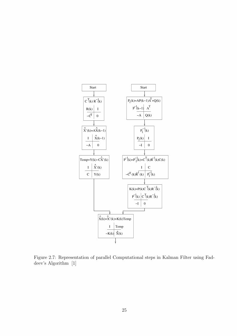
2.7 Representation of parallel Computational steps in Kalman Filter using Fad-
deev’s Algorithm [1] . . . . . . . . . . . . . . . . . . . . . . . . . . . . . . 25
2.8 Operations of Diagonal processor and off-diagonal processor in a 2 × 2
systolic array. . . . . . . . . . . . . . . . . . . . . . . . . . . . . . . . . . . 28
2.9 GR operations on rows of A . . . . . . . . . . . . . . . . . . . . . . . . . . 29
2.10 Example of Givens Rotation on a 4 × 4 matrix: Step by step procedure
showing the nullification of lower elements and thus forming the right tri-
angular matrix . . . . . . . . . . . . . . . . . . . . . . . . . . . . . . . . . 30
2.11 Functionalities of the Processing Elements (PEs) of the tri-array used as a
basic module for performing the QRD . . . . . . . . . . . . . . . . . . . . . 31
3.1 Architecture of REDEFINE . . . . . . . . . . . . . . . . . . . . . . . . . . 36
xi
3.2 Different packet formats handled by the tiles of the fabric . . . . . . . . . . 38
4.1 Schematic Diagram of Pipelined CE with enhancements over the same that
appeared in [2]. The enhancements are the inclusions of CFU and SPM to
reduce computation latency and memory latency respectively. . . . . . . . 43
4.2 Custom Instruction pipeline:HyperOp1, HYperOp2 and HyperOp3 have
established a communication among themselves, thus forming a pipeline . 45
5.1 Shaded rectangles in the figure show two neighbouring Tiles logically bound
together in a mesh interconnection . . . . . . . . . . . . . . . . . . . . . . 52
5.2 Mapping of operations and HyperOps and pHyperOps formations for the
4× 4 systolic structure . . . . . . . . . . . . . . . . . . . . . . . . . . . . . 52
5.3 Sequence of operations of HyperOps 1 and 2 of the 4× 4 systolic structure
on REDEFINE . . . . . . . . . . . . . . . . . . . . . . . . . . . . . . . . . 53
5.4 Mapping of systolic structures on REDEFINE. Grey regions depict map-
ping of systolic structure for 8×8 matrix. Hatched regions depict mapping
of systolic structure for 16×16 structure. The HyperOp sizes for those two
matrix sizes are 4× 4 and 8× 8 respectively. . . . . . . . . . . . . . . . . . 54
5.5 Realization of FP-CFU and Memory-CFU in the Compute Element . . . . 54
5.6 HyperOps and pHyperOps formation and mapping of operations and for
the 8× 8 systolic structure for QRD . . . . . . . . . . . . . . . . . . . . . 60
5.7 Critical path for a typical example of 16×16 systolic structure realization on
REDEFINE with a substructure size of 4×4, each substructure is realized
on a single CE-pair. Critical path on honeycomb is also shown on one
pHyperOp per CE basis. . . . . . . . . . . . . . . . . . . . . . . . . . . . . 66
5.8 Realization of one k×k substructure on P CE pairs . . . . . . . . . . . . . 69
5.9 For a m stage pipelined CFU, calculation of pipeline bubbles when a CISC
instruction breaks into RISC instructions. . . . . . . . . . . . . . . . . . . 70
5.10 Plots indicating the best substructure size for optimal performance in terms
of cycle-count . . . . . . . . . . . . . . . . . . . . . . . . . . . . . . . . . . 72
xii
5.11 Plots showing the normalized cycle-counts with the change in pipe-line
depth for different substructure sizes . . . . . . . . . . . . . . . . . . . . . 73
5.12 Time taken for n iterations of the critical path for problem size n×n . . . . 75
5.13 Plots indicating the best choice of the number of CE pairs to realize one
k×k substructure . . . . . . . . . . . . . . . . . . . . . . . . . . . . . . . . 76
5.14 Enhancements over FP-CFU and Memory-CFU in the Compute Element
to realize QRD kernels . . . . . . . . . . . . . . . . . . . . . . . . . . . . . 78
5.15 Part of the FSM controller that helps to break the macro-level CFU in-
struction into four RISC type instructions by generating proper control
signals for the CE set-up shown in figure 5.14. . . . . . . . . . . . . . . . . 79
xiii
List of Tables
1.1 Comparison of Representative Computing Architectures . . . . . . . . . . . 8
4.1 Matrix Multiplication: A case study (Using general compilation technique) 49
5.1 Comparison of performance with GPP and Systolic Solutions . . . . . . . . 56
5.2 The area consumed by Floating point CE with and without Custom FU is
shown . . . . . . . . . . . . . . . . . . . . . . . . . . . . . . . . . . . . . . 57
5.3 The power and area consumed by Floating point CE with Custom FUs are
reported here . . . . . . . . . . . . . . . . . . . . . . . . . . . . . . . . . . 78
xiv
Chapter 1
Introduction
In this chapter we build the foundation for the work presented in this thesis. Systolic
Array Architectures are widely accepted Application Specific Integrated Circuit (ASIC)
solutions for Numerical Linear Algebra algorithms. Starting with an overview of this
traditional solution, we gradually open the “can of worms” associated with it. We show
how Reconfigurable computing platform can serve to contain the “can of worms”. In this
context we present REDEFINE, a Coarse Grained Reconfigurable Architecture (CGRA)
for systolic actualization of Numerical Linear Algebra (NLA) kernels.
1.1 Overview of Systolic Array Solutions
A systolic array is an orchestration of pipelined processors connected in a network topol-
ogy. In systolic arrays [3, 4] the specialty is the synchronous data flow between the
processing elements, usually with particular outputs from a processing element flowing
in predefined directions and serve as inputs to other processing elements. According to
Kung and Leiserson [3], “A systolic system is a network of processors which rhythmi-
cally compute and pass data through the system”. Physiologists use the word “systole”
to refer to the rhythmically recurrent contraction of the heart and arteries which pulses
blood through the body. In a systolic computing system, the function of a processor is
analogous to that of the heart. Every processor regularly pumps data in and out, each
1
PEPE PE PE PE
PEPEPEPE
PE PE PE PE
PEPEPEPE
Inpu
t DA
TA
str
eam
sInput DATA streams
Output DATA streamsO
utpu
t DA
TA
str
eam
s
Processing Eelement
Sub−array
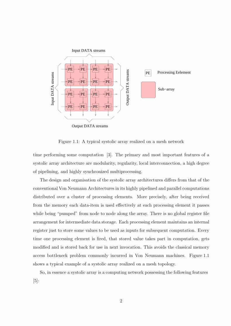
Figure 1.1: A typical systolic array realized on a mesh network
time performing some computation [3]. The primary and most important features of a
systolic array architecture are modularity, regularity, local interconnection, a high degree
of pipelining, and highly synchronized multiprocessing.
The design and organisation of the systolic array architectures differs from that of the
conventional Von Neumann Architectures in its highly pipelined and parallel computations
distributed over a cluster of processing elements. More precisely, after being received
from the memory each data-item is used effectively at each processing element it passes
while being “pumped” from node to node along the array. There is no global register file
arrangement for intermediate data storage. Each processing element maintains an internal
register just to store some values to be used as inputs for subsequent computation. Every
time one processing element is fired, that stored value takes part in computation, gets
modified and is stored back for use in next invocation. This avoids the classical memory
access bottleneck problem commonly incurred in Von Neumann machines. Figure 1.1
shows a typical example of a systolic array realized on a mesh topology.
So, in essence a systolic array is a computing network possessing the following features
[5]:
2
• Synchrony: The presence of a global clock ensures rhythmic computations and the
data produced by those computations proceed through the network.
• Modularity and regularity: Modular processing units connected in a homoge-
neous network provide the basic skeleton for any kind of systolic array architecture.
Because of structural regularity indefinite extention of the computing network is
possible.
• Spatial locality and temporal locality: The array manifests a locally-communicative
interconnection structure, i.e., spatial locality. There is at-least one cycle delay al-
loted so that signal transaction from one node to the next can be completed, i.e.,
temporal locality.
• Pipelinability: The array exhibits a linear rate pipelinability, i.e., it should achieve
an O(M) speedup, in terms of processing rate, where M is the number of Processing
Elements (PEs). Here the efficiency of the array is measured by the following:
Speedupfactor =Ts
Tp
where Ts is the processing time in a single processor, and Tp is the processing time in the
array processor.
The major factors favoring systolic arrays for special purpose processing architectures
are: simple and regular design, concurrency and communication, and balancing compu-
tation and I/O [3].
Simple and regular design: In integrated-circuit technology the cost of design
grows with the complexity of the system. By using a regular and simple design and
exploiting the Very Large Scale Integration (VLSI) technology, great savings in design
cost can be achieved. Furthermore, simple and regular systems are likely to be modular
and therefore can be adjusted to meet various performance goals.
Concurrency and Communication: An important factor that contributes to the
potential speed of a computing system is the use of concurrency. For special purpose
systems, the concurrency depends on the underlying algorithms employed by the system.
3
When a large number of processors work together, communication becomes significant.
Concurrent computations should be given more priority over the communication require-
ments while designing such a system. Systolic arrays flaunt regular and local communi-
cation among the nodes which are in concurrent execution. Thus systolic architectures
get the certification of performance advantage.
Balancing computations with I/O: A systolic array can be used as a stand-alone
ASIC solution as well as a co-processor or as an attached array processor. In both the
cases a proper balance between the computation rate and I/O rate should be maintained.
Generally as a monolithic ASIC the array works at a very high frequency while the oper-
ating frequency of the host computer, at which the data is received from and the output
is sent to, is very less in comparison. Therefore in determining the overall performance
the I/O considerations are taken into account. The ultimate performance goal is achieved
in systolic array by maintaining a computation rate that balances the available I/O band-
width with the host. To achieve this proper handshaking signals are used. And this
introduces a hint of paradigm shift from synchronous domain to asynchronous domain.
The marriage of systolic array philosophy and asynchronous data-flow computing gives
birth to wave-front array. We explore the features of wavefront arrays in forthcoming
chapters.
1.2 Numerical Linear Algebra (NLA) kernels
NLA are at the heart of all computational problems. These require hardware accelera-
tion for increased throughput as demanded by applications like high resolution direction
finding, state estimation, adaptive noise cancellation etc.
4
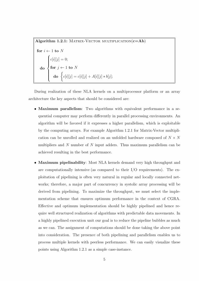
Algorithm 1.2.1: Matrix-Vector multiplication(c=Ab)
for i← 1 to N
do
c[i][j] = 0;
for j ← 1 to N
do
{c[i][j] = c[i][j] + A[i][j] ∗ b[j];
During realization of these NLA kernels on a multiprocessor platform or an array
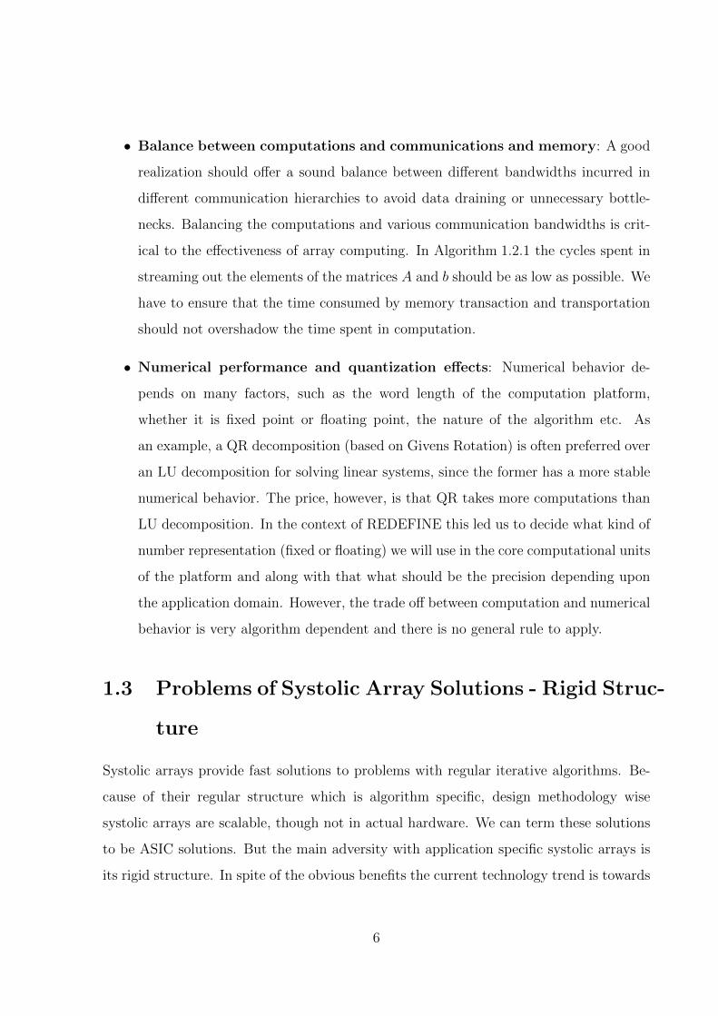
architecture the key aspects that should be considered are:
• Maximum parallelism: Two algorithms with equivalent performance in a se-
quential computer may perform differently in parallel processing environments. An
algorithm will be favored if it expresses a higher parallelism, which is exploitable
by the computing arrays. For example Algorithm 1.2.1 for Matrix-Vector multipli-
cation can be unrolled and realized on an unfolded hardware composed of N × N
multipliers and N number of N input adders. Thus maximum parallelism can be
achieved resulting in the best performance.
• Maximum pipelinability: Most NLA kernels demand very high throughput and
are computationally intensive (as compared to their I/O requirements). The ex-
ploitation of pipelining is often very natural in regular and locally connected net-
works; therefore, a major part of concurrency in systolic array processing will be
derived from pipelining. To maximize the throughput, we must select the imple-
mentation scheme that ensures optimum performance in the context of CGRA.
Effective and optimum implementation should be highly pipelined and hence re-
quire well structured realization of algorithms with predictable data movements. In
a highly pipelined execution unit our goal is to reduce the pipeline bubbles as much
as we can. The assignment of computations should be done taking the above point
into consideration. The presence of both pipelining and parallelism enables us to
process multiple kernels with peerless performance. We can easily visualize these
points using Algorithm 1.2.1 as a simple case-instance.
5
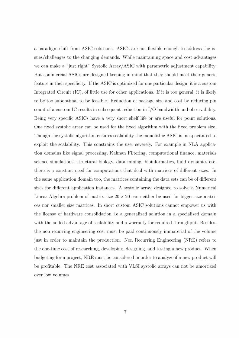
• Balance between computations and communications and memory: A good
realization should offer a sound balance between different bandwidths incurred in
different communication hierarchies to avoid data draining or unnecessary bottle-
necks. Balancing the computations and various communication bandwidths is crit-
ical to the effectiveness of array computing. In Algorithm 1.2.1 the cycles spent in
streaming out the elements of the matrices A and b should be as low as possible. We
have to ensure that the time consumed by memory transaction and transportation
should not overshadow the time spent in computation.
• Numerical performance and quantization effects: Numerical behavior de-
pends on many factors, such as the word length of the computation platform,
whether it is fixed point or floating point, the nature of the algorithm etc. As
an example, a QR decomposition (based on Givens Rotation) is often preferred over
an LU decomposition for solving linear systems, since the former has a more stable
numerical behavior. The price, however, is that QR takes more computations than
LU decomposition. In the context of REDEFINE this led us to decide what kind of
number representation (fixed or floating) we will use in the core computational units
of the platform and along with that what should be the precision depending upon
the application domain. However, the trade off between computation and numerical
behavior is very algorithm dependent and there is no general rule to apply.
1.3 Problems of Systolic Array Solutions - Rigid Struc-
ture
Systolic arrays provide fast solutions to problems with regular iterative algorithms. Be-
cause of their regular structure which is algorithm specific, design methodology wise
systolic arrays are scalable, though not in actual hardware. We can term these solutions
to be ASIC solutions. But the main adversity with application specific systolic arrays is
its rigid structure. In spite of the obvious benefits the current technology trend is towards
6
a paradigm shift from ASIC solutions. ASICs are not flexible enough to address the is-
sues/challenges to the changing demands. While maintaining space and cost advantages
we can make a “just right” Systolic Array/ASIC with parametric adjustment capability.
But commercial ASICs are designed keeping in mind that they should meet their generic
feature in their specificity. If the ASIC is optimized for one particular design, it is a custom
Integrated Circuit (IC), of little use for other applications. If it is too general, it is likely
to be too suboptimal to be feasible. Reduction of package size and cost by reducing pin
count of a custom IC results in subsequent reduction in I/O bandwidth and observability.
Being very specific ASICs have a very short shelf life or are useful for point solutions.
One fixed systolic array can be used for the fixed algorithm with the fixed problem size.
Though the systolic algorithm ensures scalability the monolithic ASIC is incapacitated to
exploit the scalability. This constrains the user severely. For example in NLA applica-
tion domains like signal processing, Kalman Filtering, computational finance, materials
science simulations, structural biology, data mining, bioinformatics, fluid dynamics etc.
there is a constant need for computations that deal with matrices of different sizes. In
the same application domain too, the matrices containing the data sets can be of different
sizes for different application instances. A systolic array, designed to solve a Numerical
Linear Algebra problem of matrix size 20× 20 can neither be used for bigger size matri-
ces nor smaller size matrices. In short custom ASIC solutions cannot empower us with
the license of hardware consolidation i.e a generalized solution in a specialized domain
with the added advantage of scalability and a warranty for required throughput. Besides,
the non-recurring engineering cost must be paid continuously immaterial of the volume
just in order to maintain the production. Non Recurring Engineering (NRE) refers to
the one-time cost of researching, developing, designing, and testing a new product. When
budgeting for a project, NRE must be considered in order to analyze if a new product will
be profitable. The NRE cost associated with VLSI systolic arrays can not be amortized
over low volumes.
7
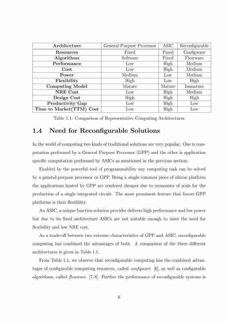
Architecture General Purpose Processor ASIC Reconfigurable
Resources Fixed Fixed ConfigwareAlgorithms Software Fixed Flowware
Performance Low High MediumCost Low High Medium
Power Medium Low MediumFlexibility High Low High
Computing Model Mature Mature ImmatureNRE Cost Low High Medium
Design Cost High High HighProductivity Gap Low High Low
Time to Market(TTM) Cost Low High Low
Table 1.1: Comparison of Representative Computing Architectures
1.4 Need for Reconfigurable Solutions
In the world of computing two kinds of traditional solutions are very popular. One is com-
putation performed by a General Purpose Processor (GPP) and the other is application
specific computation performed by ASICs as mentioned in the previous section.
Enabled by the powerful tool of programmability any computing task can be solved
by a general-purpose processor or GPP. Being a single common piece of silicon platform
the applications hosted by GPP are rendered cheaper due to economics of scale for the
production of a single integrated circuit. The most prominent feature that favors GPP
platforms is their flexibility.
An ASIC, a unique function solution provider delivers high performance and low power
but due to its fixed architecture ASICs are not suitable enough to meet the need for
flexibility and low NRE cost.
As a trade-off between two extreme characteristics of GPP and ASIC, reconfigurable
computing has combined the advantages of both. A comparison of the three different
architectures is given in Table 1.1.
From Table 1.1, we observe that reconfigurable computing has the combined advan-
tages of configurable computing resources, called configware [6], as well as configurable
algorithms, called flowware [7, 8]. Further the performance of reconfigurable systems is
8

better than general-purpose systems and the cost is less than that of ASICs. Recon-
figurable platforms entrust us with the power of hardware consolidation. Only recently
the power consumption of reconfigurable systems has been improved such that it is now
either comparable with ASICs or even smaller due to hardware consolidation. The main
advantage of the reconfigurable system lies in its high flexibility, while its main restraint
is the lack of a standard computing model. The design effort in terms of NRE cost i.e the
chip fabrication cost is in between that of general-purpose processors and ASICs. The
other two axes of direct costs are Design Cost and Productivity Gap. The design cost
crops up from the efforts encountered while developing the application and envisioning
the architecture. For reconfigurable platforms the application development cost is same
as that of a GPP. Though design of the architecture brings in a high cost for the first time,
but it amortizes with multiple applications to be accommodated by the platform. Use of
compilers helps in transforming the circuit description from higher level of abstraction to
a lower level, usually towards physical implementation. Thus, GPPs and Reconfigurable
Platforms bridge the Productivity Gap which creates a lacuna between design complexity
and design capacity in case of ASICs. Reconfigurable Platforms also can be seen as viable
vehicles towards reducing the time-to-market costs.
There exists systolic array solutions for NLA kernels. While such custom hardware
solutions for NLA Solvers can deliver high performance, they are not scalable. In our work,
we show how NLA kernels can be realized on REDEFINE [9,10], a runtime reconfigurable
hardware platform. The two kernels we use as running example are Modified Faddeev’s
Algorithm [11] and QR decomposition using Givens Rotation [12]. REDEFINE is a
CGRA combining the flexibility of a programmable solution with the execution speed
of an ASIC. The solution proposed here is capable of emulating systolic arrays over a
wide variety of NLA problem sizes. In REDEFINE Compute Elements are arranged in a
honeycomb topology connected via a Network on Chip (NoC) called RECONNECT, to
realize the various macro-functional blocks of an equivalent ASIC. Architectural details
of REDEFINE are presented in subsequent sections. We propose a few enhancements
to improve the performance of REDEFINE in the context of NLA kernels. Along with
9
the actualization details of the afore-mentioned kernels we explore the design space of
the proposed solutions. These can be treated as specific examples for the realization of
all decomposition type algorithms. We show how REDEFINE meets both the scalability
and performance requirements of NLA kernels. We further show the scalability of the
architecture by taking increasing problem sizes but without altering the improvement in
performance.
1.5 Our Contribution
In this thesis we present how the traditional systolic solutions for NLA kernels can be
re-targeted for realization on REDEFINE, a runtime reconfigurable platform with appro-
priate mapping of the nodes of the systolic array. REDEFINE is a coarse grain reconfig-
urable architecture, where the elementary schedulable unit is HyperOp [13]. HyperOps
are a subgraph of the application dataflow graph comprising a set of elementary operations
that have strong producer-consumer relationship. In REDEFINE, an application speci-
fied in a high level language C is compiled into HyperOps. Each HyperOp contains the
meta-data that specifies its computation and communication requirements. Configuration
information captured in the meta-data is generated statically by the compiler. Hardware
resources in the REDEFINE fabric are dynamically provisioned for HyperOps executed at
runtime. Application synthesis in REDEFINE follows a compilation process in which an
application specified in C is translated into a dataflow graph as an intermediate represen-
tation. Subgraphs of this Dataflow graph form HyperOps. HyperOps are coarse grained
application substructures that are staged for execution on REDEFINE following a data
driven schedule. In order to exploit instruction level parallelism hyperOps are further
divided into partitioned hyperOps, pHyperOps in short. pHyperOps contain the compute
and transport metadata capturing the computation and communication requirements of
the application. Hence, the compilation process [13] is divided into the various phases i.e,
Formation of DFG, HyperOp formation, Tag generation, Mapping HyperOps
and Formation of Custom Instructions. Detailed descriptions of the compilation
process are available in [13]. From the dataflow graph HyperOps and pHyperOps are
10
created for data driven execution in the CEs [13] maintaining some semantics. But the
main problem associated with this is that the HyperOps formations are algorithm ag-
nostic. The same is true when the compiler passes through the mapping phase. Hence,
for certain algorithms eg. NLA kernels, this generic approach of HyperOp creation and
mapping does not culminate into the achievable optimum performance. The aim of the
work presented here is to obtain a theoretical basis to enable algorithm aware HyperOp
creation, and arriving at pHyperOps that can be optimally mapped to CEs. We take
the systolic array solutions mostly realized on mesh topology as our source graph and
map them on a target graph of honeycomb topology. We partition the whole array into
multiple sub-arrays (refer figure 1.1) and call them HyperOps. Depending upon the size
of the sub-arrays computational resources are assigned to them. We determine the right
size of the sub-array in accordance with the optimal pipeline depth of the core execution
units (Compute Element (CE)s) and the number of such units to be used per sub-array.
Such a solution will allow emulation of systolic structures on REDEFINE ushering the
way for optimal performance.
1.6 Thesis Overview
This thesis has been organized as follows:
Chapter 2 builds the foundation stone of systolic computing paradigm. Then the
chapter reviews the specific systolic algorithms that we have realized on REDEFINE. The
two algorithms discussed here are Modified Faddeev’s Algorithm (Direct Solver) and QR
Decomposition (QRD) using Givens Rotation. The benefits of QRD over LU Decompo-
sition is also highlighted here.
Chapter 3 presents the overall architecture of REDEFINE framework.
Chapter 4 advocates QRD and other NLA-specific enhancements to REDEFINE in
order to meet expected performance goals.
Chapter 5 traces the realization details of Systolic Architectures onto REDEFINE.
Here we propose the framework for algorithm aware HyperOp, generation of their parti-
tions into pHyperOps for desired mapping on a set of CEs. We further do design space
11
exploration of the contemplated solution. We present the theoretical results also to make
a fair performance comparison of the solution to that of an GPP.
Chapter 6 manifests the detailed hardware architecture of the common core compu-
tational units of REDEFINE. The synthesis results are also reported.
Chapter 7 concludes the thesis with avenues for further work.
12
Chapter 2
Systolic Algorithms
Most of the algorithms used in signal and image processing exhibit features like localized
operations, intensive computation and matrix operations. The design approach of special-
purpose signal and image processing array processors completely relies on the exploitation
of these common features of the algorithms. Expression and transformation of this special
class of algorithms play an important role in the initial phase of design. For parallel and
pipeline processing algorithm expression provides the foundation stone for realization of a
more systematic and formal description such as a dependence graph. Among many efforts
towards developing a formal description of the space-time activities in array-processors
[3, 14] the most natural approach is to describe the actual space-time activities in terms
of snapshots that display data activities at a particular time instant.
In this chapter we talk about the main considerations in providing a formal and
powerful description(expression) of any algorithm, the systematic method to transform
an algorithm description to an array processor and how to optimize the performance of
those parallel algorithms realized on the arrays. Detailed descriptions are given in [5].
For reader’s convenience the some of the salient features have been reproduced here in a
nutshell.
13
2.1 Parallel algorithm Expression
Parallel algorithm expressions may be derived by two approaches:
• Vectorization of sequential algorithm expressions
• Direct parallel algorithm expressions, such as snapshots, recursive equations, parallel
codes, single assignment code, dependence code, dependence graphs and so on.
2.1.1 Vectorization of Sequential Algorithm Expressions:
High level languages like C provide concise algorithm expression and have been used as
machine independent programming tools. Programming in these sequential languages
requires the decomposition of an algorithm into sequence of steps, each of which performs
an operation on a scalar object. For example, consider a mathematical expression of the
matrix addition C = A+B:
C(i, j) = A(i, j) +B(i, j), ∀ i and j (2.1)
The corresponding pseudo-code for C code can be written as
Algorithm 2.1.1: Matrix-Matrix addition(C=A+B)
for i← 1 to N
do
for j ← 1 to N
do
{C[i][j] = A[i][j] +B[i][j];
Here the elements of A and B are accessed in column major order, which by definition,
is the order in which they are stored. Many computers may not be able to execute the
program as efficiently if the order is reversed. In this example, as no ordering is required
by the algorithm, it is unwise to encode an ordering in the program.
If no ordering is encoded, the compiler may choose the most efficient ordering for the
target computer. Moreover, should the target computer contain parallelism, then some or
14
all of the operations may be performed concurrently, without analysis or ambiguity. Since
ordering is unavoidable when using sequential code, parallel expression of an algorithm is
very desirable.
2.1.2 Direct Expressions of Parallel Algorithms:
Extracting the inherent concurrency(parallel and pipeline) of any given program may not
be always done effectively by a vectorizing compiler. Hence, it is advantageous that a
user/designer use parallel expressions to describe an algorithm in the first place. This
is the key step leading to an algorithm-oriented array processor design. Many different
expressions may be used to represent a parallel algorithm, including snapshots, recursive
algorithms with space time indices, parallel codes, Dependence Graph (DG)s, or Signal
Flow Graph (SFG)s.
Single Assignment Code: A single assignment code is a form where every variable
is assigned one value only during the execution of the algorithm.
Recursive Algorithms: A convenient and concise expression for the representation
of many algorithms is to use recursive equations. The recursive equation for the matrix-
vector multiplication c = Ab is:
c(j+1)i = c
(j)i + aji b
(j)i , ∀ i and j (2.2)
where j is the recursion index, j = 1, 2, · · · , N, and
c(1)i = 0 (2.3)
a(j)i = A(i, j) (2.4)
b(j)i = B(j) (2.5)
A recursive equation with space-time indices uses one index for time and the other
indices for space. By doing so, the activities of a parallel algorithm can be adequately
expressed. The preceding equation can be viewed as a recursive equation with the j-index
15
A31
A41
A12
A22A32
A13
A23
A31
A41
A22
A32
A13
A23A14
A14
A B(2)12
A B(1)11
A B(1)21
A B(1)11
A11
A21
A31
A41
A13
A23
A22
A12
A32
A21
B(4) B(3) B(2) B(1)
B(4) B(3) B(2) B(1)
14
B(4) B(3) B(2) B(1)
A
+
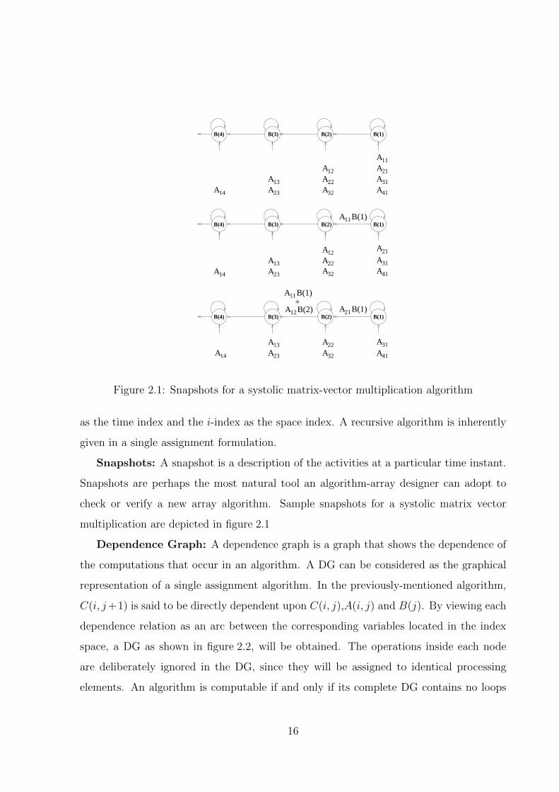
Figure 2.1: Snapshots for a systolic matrix-vector multiplication algorithm
as the time index and the i-index as the space index. A recursive algorithm is inherently
given in a single assignment formulation.
Snapshots: A snapshot is a description of the activities at a particular time instant.
Snapshots are perhaps the most natural tool an algorithm-array designer can adopt to
check or verify a new array algorithm. Sample snapshots for a systolic matrix vector
multiplication are depicted in figure 2.1
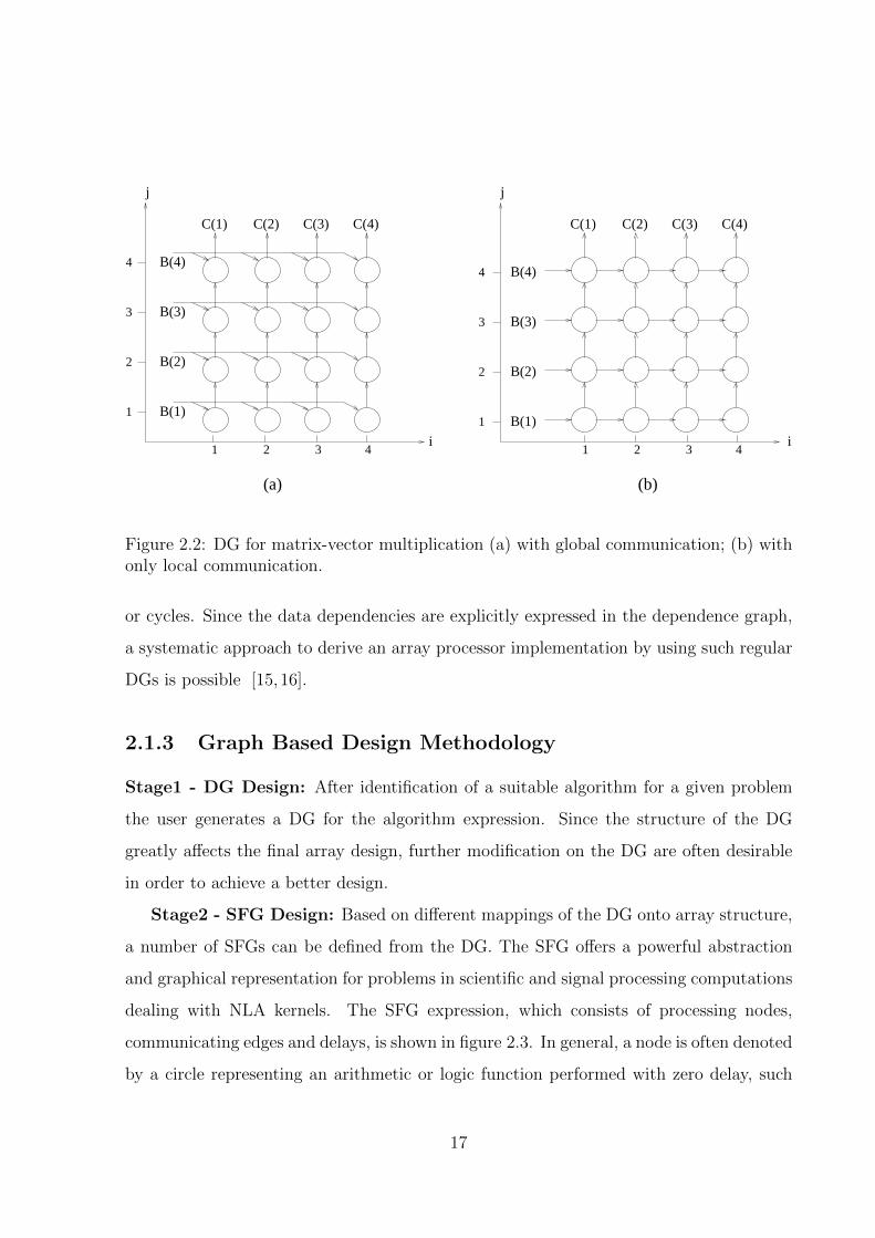
Dependence Graph: A dependence graph is a graph that shows the dependence of
the computations that occur in an algorithm. A DG can be considered as the graphical
representation of a single assignment algorithm. In the previously-mentioned algorithm,
C(i, j+1) is said to be directly dependent upon C(i, j),A(i, j) and B(j). By viewing each
dependence relation as an arc between the corresponding variables located in the index
space, a DG as shown in figure 2.2, will be obtained. The operations inside each node
are deliberately ignored in the DG, since they will be assigned to identical processing
elements. An algorithm is computable if and only if its complete DG contains no loops
16
B(1)
B(2)
B(3)
B(4)
C(1) C(2) C(3) C(4)
4
3
2
1
4
3
2
1
1 2 3 41 2 3 4
B(1)
B(2)
B(3)
B(4)
C(1) C(2) C(3) C(4)
j
i
j
i
(a) (b)
Figure 2.2: DG for matrix-vector multiplication (a) with global communication; (b) withonly local communication.
or cycles. Since the data dependencies are explicitly expressed in the dependence graph,
a systematic approach to derive an array processor implementation by using such regular
DGs is possible [15,16].
2.1.3 Graph Based Design Methodology
Stage1 - DG Design: After identification of a suitable algorithm for a given problem
the user generates a DG for the algorithm expression. Since the structure of the DG
greatly affects the final array design, further modification on the DG are often desirable
in order to achieve a better design.
Stage2 - SFG Design: Based on different mappings of the DG onto array structure,
a number of SFGs can be defined from the DG. The SFG offers a powerful abstraction
and graphical representation for problems in scientific and signal processing computations
dealing with NLA kernels. The SFG expression, which consists of processing nodes,
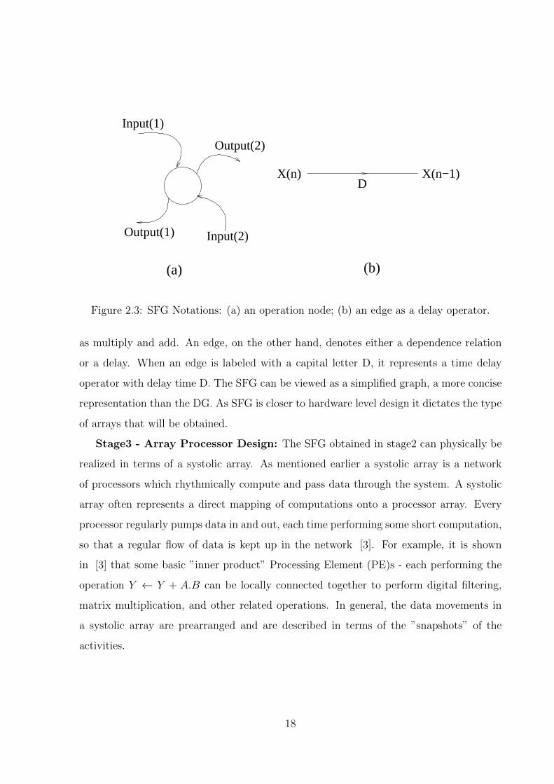
communicating edges and delays, is shown in figure 2.3. In general, a node is often denoted
by a circle representing an arithmetic or logic function performed with zero delay, such
17
Input(1)
Input(2)
Output(2)
Output(1)
X(n−1)
(a) (b)
X(n)D
Figure 2.3: SFG Notations: (a) an operation node; (b) an edge as a delay operator.
as multiply and add. An edge, on the other hand, denotes either a dependence relation
or a delay. When an edge is labeled with a capital letter D, it represents a time delay
operator with delay time D. The SFG can be viewed as a simplified graph, a more concise
representation than the DG. As SFG is closer to hardware level design it dictates the type
of arrays that will be obtained.
Stage3 - Array Processor Design: The SFG obtained in stage2 can physically be
realized in terms of a systolic array. As mentioned earlier a systolic array is a network
of processors which rhythmically compute and pass data through the system. A systolic
array often represents a direct mapping of computations onto a processor array. Every
processor regularly pumps data in and out, each time performing some short computation,
so that a regular flow of data is kept up in the network [3]. For example, it is shown
in [3] that some basic ”inner product” Processing Element (PE)s - each performing the
operation Y ← Y + A.B can be locally connected together to perform digital filtering,
matrix multiplication, and other related operations. In general, the data movements in
a systolic array are prearranged and are described in terms of the ”snapshots” of the
activities.
18
1
2
3
45 6 7
S (Normal Vector)
Hyp
erpl
anes
(a) (b)
Projection Vector
d
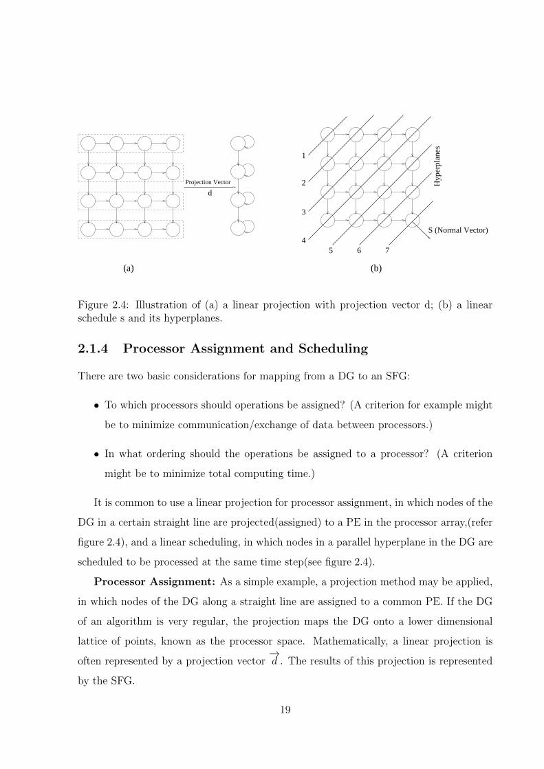
Figure 2.4: Illustration of (a) a linear projection with projection vector d; (b) a linearschedule s and its hyperplanes.
2.1.4 Processor Assignment and Scheduling
There are two basic considerations for mapping from a DG to an SFG:
• To which processors should operations be assigned? (A criterion for example might
be to minimize communication/exchange of data between processors.)
• In what ordering should the operations be assigned to a processor? (A criterion
might be to minimize total computing time.)
It is common to use a linear projection for processor assignment, in which nodes of the
DG in a certain straight line are projected(assigned) to a PE in the processor array,(refer
figure 2.4), and a linear scheduling, in which nodes in a parallel hyperplane in the DG are
scheduled to be processed at the same time step(see figure 2.4).
Processor Assignment: As a simple example, a projection method may be applied,
in which nodes of the DG along a straight line are assigned to a common PE. If the DG
of an algorithm is very regular, the projection maps the DG onto a lower dimensional
lattice of points, known as the processor space. Mathematically, a linear projection is
often represented by a projection vector−→d . The results of this projection is represented
by the SFG.
19
Scheduling: Scheduling scheme specifies the sequence of operations in all the PEs.
A schedule function represents a mapping from the N-dimensional index space of the
DG onto a 1-D schedule(time) space. A linear schedule is based on a set of parallel
and uniformly spaced hyperplanes in the DG. These hyperplanes are called equitemporal
hyperplanes, i.e all the nodes on the same hyperplane must be processed at the same
time. Mathematically, the schedule can be represented by a (column) schedule vector −→s ,
pointing to the normal direction of the hyperplanes.
Permissible Linear Schedule: Given a DG and a projection direction−→d , we note
that not all the hyperplanes qualify to define a valid schedule for the DG. In order for the
given hyperplanes to represent a permissible linear schedule, it is necessary and sufficient
that the normal vector −→s satisfies the following two conditions:
−→s T−→e ≥ 0, for any dependence arc −→e . (2.6)
−→s T−→d > 0. (2.7)
Both the conditions 2.6 and 2.7 can be checked by inspection. In short, the schedule is
permissible if and only if
• all the dependency arcs flow in the same direction across the hyperplanes and
• the hyperplanes are not parallel with the projection vector−→d .
The first condition means that a causality should be enforced in a permissible schedule.
Namely, if node p depends on node q, then the time step assigned for p can not be less than
the time step assigned for q. The second condition implies that nodes on an equitemporal
hyperplane should not be projected to the same PE.
20
2.2 Systolic Solutions for Numerical Linear Algebra
kernels
Application domains such as Bio-informatics, Digital Signal Processing (DSP), Structural
Biology, Fluid Dynamics etc. demand high performance computing solutions for their
simulation environments. The core computations of these applications is in Numerical
Linear Algebra (NLA) kernels. These kernels need to be executed taking the nature of
the target application into consideration. Direct solvers are predominantly required in the
domains like DSP, estimation algorithms like Kalman Filter [1] etc, where the matrices
on which operations need to be performed are either small or medium sized, but dense.
Here in this section we show how Faddeevs Algorithm [17] can be used as a direct solver.
We further talk about QR Decomposition of any matrix, often used to solve the linear
least square problem. Systolic realizations of both the kernels are presented.
2.2.1 Faddeev’s Algorithm
Faddeevs Algorithm (FA) [17] is used for solving dense linear system of equations. FA [1]
enables us to compute the Schur complement of a compound matrix M (composed of
four matrices A, B, C, D of sizes (n×n), (n×l), (m×n), (m×l) respectively, provided
A is non-singular [18]. A variant of this algorithm that is amenable for realization in
hardware was proposed by Nash et al. [11]. This is referred to as the Modified Faddeevs
algorithm (MFA). Calculation of Schur complement [D + CA−1B] using MFA, which
in effect, is a two step process i.e triangularization of matrix A and nullification of the
elements of matrix C [19].
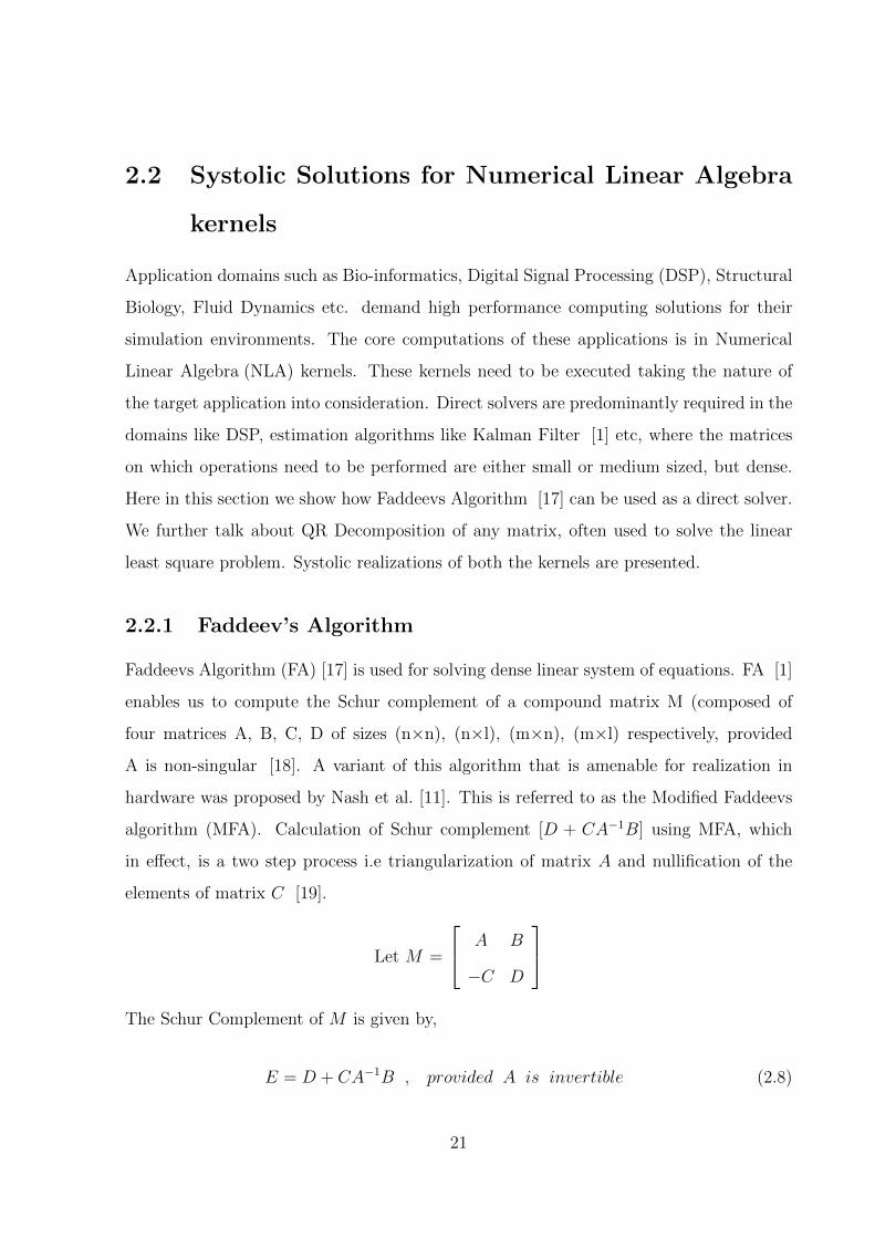
Let M =
A B
−C D
The Schur Complement of M is given by,
E = D + CA−1B , provided A is invertible (2.8)
21
The representation of E in matrix form is as follows (for a typical case of 2× 2):
e11 e12
e21 e22
=
d11 d12
d21 d22
+
c11 c12
c21 c22
a11 a12
a21 a22
−1 b11 b12
b21 b22
(2.9)
Systolic array with their regular lattice structure provides a good parallel platform to
realize the calculation of Schur Complement in hardware. For systolic realization of MFA,
the desired lattice is a mesh interconnection of CEs. In subsequent sections we will see
how REDEFINE can provide a reconfigurable and scalable solution for the calculation of
Schur Complement using MFA.
2.2.2 Brief description of the algorithm
To illustrate Faddeev’s algorithm consider the simple case of computing:
C1X1 + C2X2 + C3X3 + · · · · · ·+ CnXn + d (2.10)
where C1, C2, C3 · · · Cn are given numbers, and X1, X2, X3 · · · Xn are the solution to
the linear system of equations
a11X1 + a12X2 + a13X3 + · · · · · ·+ a1nXn = b1
a21X1 + a22X2 + a23X3 + · · · · · ·+ a2nXn = b2
a31X1 + a32X2 + a33X3 + · · · · · ·+ a3nXn = b3
· · · · · · (2.11)
· · · · · ·
an1X1 + an2X2 + an3X3 + · · · · · ·+ annXn = bn
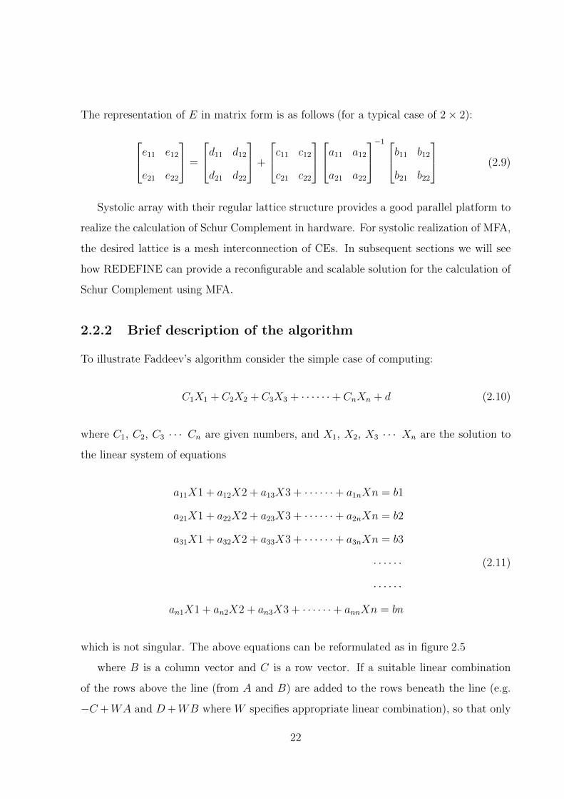
which is not singular. The above equations can be reformulated as in figure 2.5
where B is a column vector and C is a row vector. If a suitable linear combination
of the rows above the line (from A and B) are added to the rows beneath the line (e.g.
−C +WA and D+WB where W specifies appropriate linear combination), so that only
22
a11 a12
a21 a22
an1 an2
a1n
a2n
ann
b1
b2
bn
d−c n−c 1 −c 2or
ADB
−C
Figure 2.5: Faddeev’s Algorithm deals with an augmented matrix of four different matrices
zeroes appear in the lower left hand quadrant, then the desired result, CX+D will appear
in the lower right quadrant. This follows because the annulment of the lower left hand
quadrant requires that
W = CA−1 (2.12)
so that
D +WB = D + CA−1B (2.13)
Since, X = A−1B, we have the final result
D +WB = D + CX (2.14)
Identification of the multipliers of the rows of A and elements of B is not required; it is
only necessary to annul the last row. This can be done by ordinary Gaussian elimination.
The triangularization of matrix A is done as traditional LU Decomposition. A brief
mathematical insight of LU Decomposition is elucidated in the next section. An important
feature of this algorithm is that it avoids the usual back substitution solution to the
triangular linear system and obtains the values of the unknowns directly at the end of
the forward course of computation, resulting in considerable savings in processing and
storage. Statistical studies have shown that the numerical accuracy is comparable to the
usual LU decomposition and back substitution. This result can be generalized in case of
rectangular matrices C, D and B. After the lower left hand quadrant is annulled, the
23
BA
−I 0
ABD − CA B−1
BA
C D
CB
B
−C D
I
BA
0−I
−1A B
BA
D−C
−1D + CA B
A I
−I 0
A−1
CA + D−1
D
I
−C
A
A B + D−1
BA
D−I
A
−1
0−C
I
CA
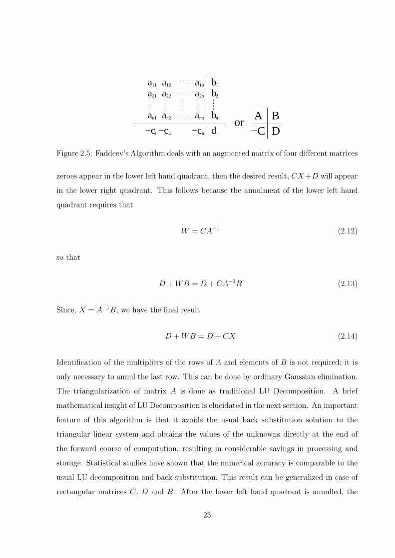
Figure 2.6: Different possible Matrix-Solutions using MFA
result CA−1B + D will appear in the lower right hand quadrant. The numerous matrix
operations possible by selective entries in the four quadrants are as shown in figure 2.6).
Nash and Hassan [11] have modified FA by introducing orthogonal factorization ca-
pability. This leads to more numerical stability. We adopt the MFA algorithm in our
work. Different possible results could be obtained by feeding different matrices in place of
A, B, C and D. Each result has two or more matrix operations combined together into a
single operation. Moreover, matrix inversion is straightforward. These properties can be
exploited to reduce the computation involved in the Kalman filter [1] equations. Compu-
tational steps in these equations [1] (refer figure 2.7) can be decomposed into many sub
tasks each of which can be executed in a step using FA.
24
Start Start
^
^
^X’(k)=AX(k−1)
X(k−1)
0
I
−A
I
C
X’(k)
Y(k)
^
^Temp=Y(k)−CX’(k)
IP (k)
P (k)−1
1
1
−I 0
1
P (k)=P (k)+C (k)R (k)C(k)−1
1
I C
−1P (k)−C (k)R (k)
−1
T
−1
−1
T
X(k)−K(k)
I Temp
^
^
^X(k)=X’(k)+K(k)Temp
C (k) R (k)T −1
R(k)
−C
I
0T
TP (k)=AP(k−1)A +Q(k)1
−A
A
Q(k)
TP (k−1)
K(k)=P(k)C (k)R (k)T −1
C (k)R (k)
0
T −1
−I
P (k)−1
−1
Figure 2.7: Representation of parallel Computational steps in Kalman Filter using Fad-deev’s Algorithm [1]
25
2.2.3 LU Decomposition
Let A be an n × n square matrix. A can be decomposed into unit lower triangular and
upper triangular matrices [20] as shown below
A = LU (2.15)
where L and U are lower and upper triangular matrices (of the same size i.e n × n)
respectively. For a 3× 3 matrix:a11 a12 a13
a21 a22 a23
a31 a32 a33
=
1 0 0
l21 1 0
l31 l32 1
u11 u12 u13
u21 u22 0
u31 0 0
(2.16)
Upon multiplying the two matrices L and U get,a11 a12 a13
a21 a22 a23
a31 a32 a33
=
u11 u12 u13
l21u11 + u21 l21u12 + u22 l21u13
l31u11 + l32u21 + u31 l31u12 + l32u22 l31u13
(2.17)
Hence by comparing the matrices on element by element basis we get,
u11 = a11, u12 = a12, u13 = a13 (2.18)
l21 =a23u13
, l31 =a33u13
(2.19)
u22 = a22 − l21u12, u21 = a21 − l21u11 (2.20)
l32 =a32 − l31u12
u22, u31 = a31 − l31u11 − l32u21 (2.21)
26
If we observe with attention we can form two generalized equations to get the non-zero
elements of the lower (L) and upper (U) triangular matrices as:
lij =aij −
∑j−1k=1 likukjujj
(2.22)
uij = aij −i−1∑k=1
likukj (2.23)
The elements of the U and L matrix are uniquely determined on applying the above
mentioned equations in the correct order.
2.2.4 Systolic Array realization
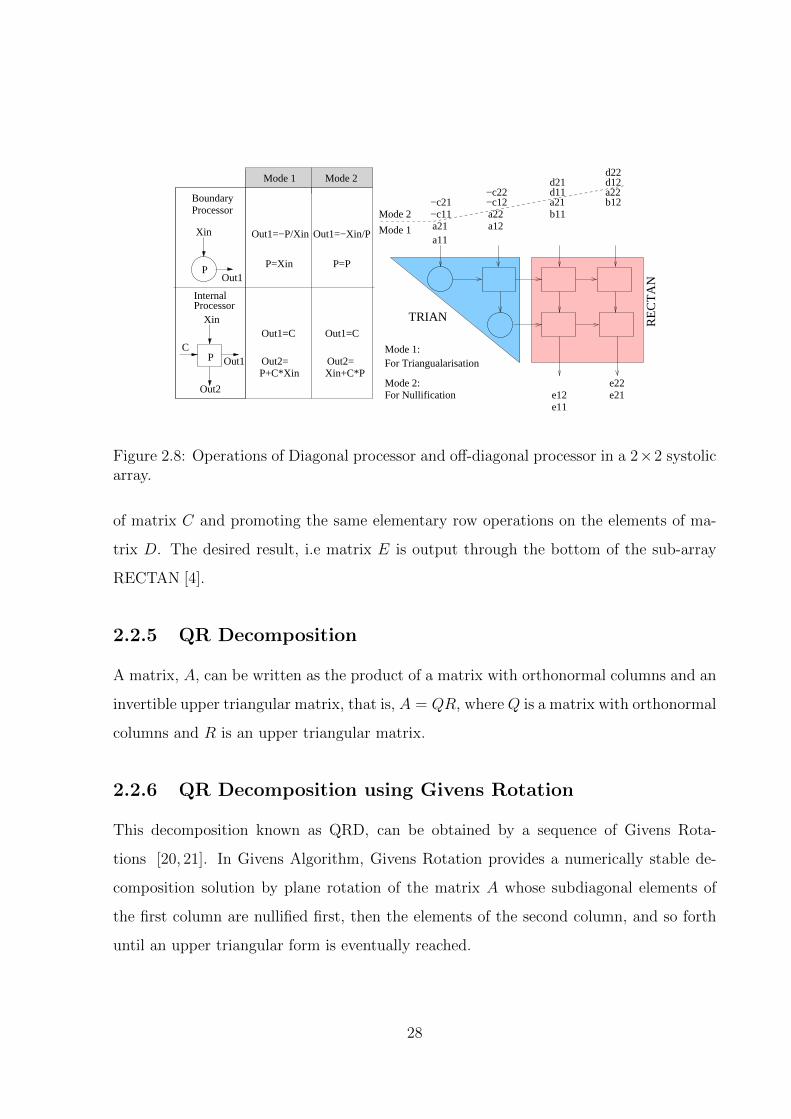
The trapezoidal array illustrated in figure 2.8. is the most popular systolic array imple-
mentation of the Faddeevs algorithm. If the input matrices are of size n × n, then the
Systolic array is made up of a triangular segment i.e sub-array TRIAN and a rectangular
segment i.e sub-array RECTAN. These two sub-arrays contain n(n−1)/2 and n2 number
of Processing Elements (PEs), respectively. There are two types of PE : Diagonal and
Off-diagonal PE. The input-output signatures of the two kinds of PEs are shown in fig-
ure 2.8. As shown in the figure 2.8, the elements of matrix A and B are first fed to the
sub-arrays TRIAN and RECTAN respectively but in a skewed manner. This skewing is
achieved through delay cells. The elements of matrix A are triangularized in the sub-array
TRIAN, then are stored in the PEs of that sub-array. At the same time, the factors for
elementary row operations are fed to the right-hand sub-array RECTAN, and the same
row elements of B encounter the same transformations, and stored back in the internal
registers of the PEs of sub-array RECTAN. Continuing the flow, elements of matrices C
and D are fed to the triangular and rectangular segments of the trapezoidal array respec-
tively. All the processing elements works in dual mode. Mode 1 is for operations related
to the triangularization of matrix A and subsequent operations on the elements of matrix
B. In mode 2 Processing elements perform operation pertaining to nullify the elements
27
P
e22e21e12
e11
a11a21 a12
a22 b11b12a22
a21d11d21 d12
d22
−c11−c21 −c12
−c22
Mode 2
Mode 1
Out1
Xin
InternalProcessor
Xin
Out1
Out2
BoundaryProcessor
P=Xin
Out1=−P/Xin
COut1=C
Out2= Out2=P+C*Xin
Out1=C
Out1=−Xin/P
P=P
Mode 2Mode 1
Xin+C*P
P
For NullificationMode 2:
For TriangualarisationMode 1:
RE
CT
AN
TRIAN
Figure 2.8: Operations of Diagonal processor and off-diagonal processor in a 2×2 systolicarray.
of matrix C and promoting the same elementary row operations on the elements of ma-
trix D. The desired result, i.e matrix E is output through the bottom of the sub-array
RECTAN [4].
2.2.5 QR Decomposition
A matrix, A, can be written as the product of a matrix with orthonormal columns and an
invertible upper triangular matrix, that is, A = QR, where Q is a matrix with orthonormal
columns and R is an upper triangular matrix.
2.2.6 QR Decomposition using Givens Rotation
This decomposition known as QRD, can be obtained by a sequence of Givens Rota-
tions [20, 21]. In Givens Algorithm, Givens Rotation provides a numerically stable de-
composition solution by plane rotation of the matrix A whose subdiagonal elements of
the first column are nullified first, then the elements of the second column, and so forth
until an upper triangular form is eventually reached.
28
(q,p)Q = 0
0
0
0−sin
pth
colu
mn
(p+
1)
st
c
olum
n
1
1
1
0
0
0 0
0 0
0 0
0 0
0 0
0 0
0
1
0
0 0
0 0
. . . . . . . . . . . . . . .
. . . . . . . . . . . . . . .
. . . . . . . . . . . . . . .
. . . . . . . . . . . . .
. . . . . . . . . . . . .
. . . . . . . . . . . .
. . . . . .
cos sin
cos
..
..
st
thq row
(q+1) row
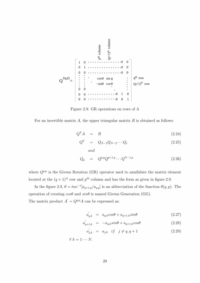
Figure 2.9: GR operations on rows of A
For an invertible matrix A, the upper triangular matrix R is obtained as follows:
QTA = R (2.24)
QT = QN−1QN−2 · · ·Q1 (2.25)
and
Qp = Qp,pQp+1,p · · ·QN−1,p (2.26)
where Qq,p is the Givens Rotation (GR) operator used to annihilate the matrix element
located at the (q + 1)st row and pth column and has the form as given in figure 2.9.
In the figure 2.9, θ = tan−1[aq+1,p/aq,p] is an abbreviation of the function θ(q, p). The
operation of creating cosθ and sinθ is named Givens Generation (GG).
The matrix product A′= Qq,pA can be expressed as:
a′
q,k = aq,kcosθ + aq+1,ksinθ (2.27)
a′
q+1,k = −aq,ksinθ + aq+1,kcosθ (2.28)
a′
j,k = aj,k if j 6= q, q + 1 (2.29)
∀ k = 1 · · ·N.
29
X X X X
X X X X
X X X X
X X X X
X X X X
X X
X X X
X X X0
0
0 0
X X X X
X X X X
X X X X
X X X0
X X X X
X X X X
X X X
X X X
0
0
X X X X
X X X
X X X
X X X0
0
0
X X X X
X X
X X
X X X0
0
0
0
0
X X X X
X X X
X X
X
0
0
0
0
0 0
GR(41) GR(31) GR(21)
GR(42) GR(32) GR(43)
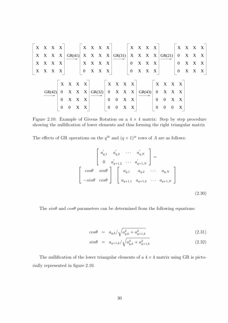
Figure 2.10: Example of Givens Rotation on a 4 × 4 matrix: Step by step procedureshowing the nullification of lower elements and thus forming the right triangular matrix
The effects of GR operations on the qth and (q + 1)st rows of A are as follows:
a′q,1 a
′q,2 · · · a
′q,N
0 a′q+1,2 · · · a
′q+1,N
=
cosθ sinθ
−sinθ cosθ
aq,1 aq,2 · · · aq,N
aq+1,1 aq+1,2 · · · aq+1,N
(2.30)
The sinθ and cosθ parameters can be determined from the following equations:
cosθ = aq,k/√a2q,k + a2q+1,k (2.31)
sinθ = aq+1,k/√a2q,k + a2q+1,k (2.32)
The nullification of the lower triangular elements of a 4× 4 matrix using GR is picto-
rially represented in figure 2.10.
30
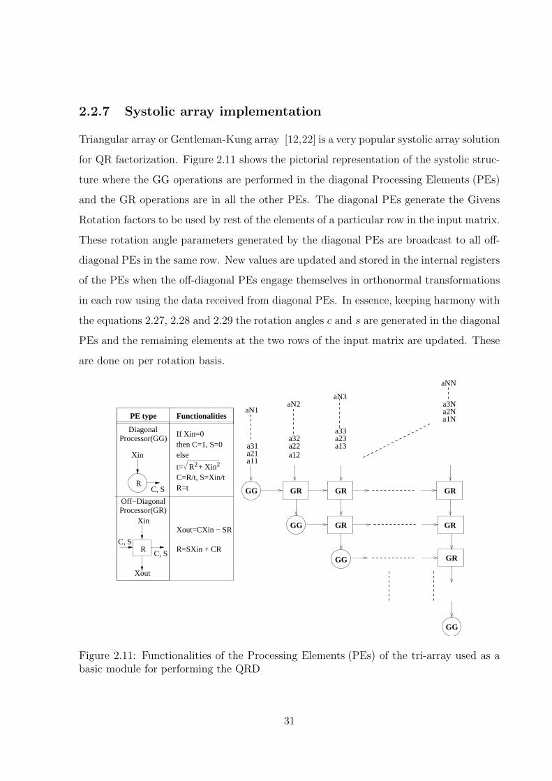
2.2.7 Systolic array implementation
Triangular array or Gentleman-Kung array [12,22] is a very popular systolic array solution
for QR factorization. Figure 2.11 shows the pictorial representation of the systolic struc-
ture where the GG operations are performed in the diagonal Processing Elements (PEs)
and the GR operations are in all the other PEs. The diagonal PEs generate the Givens
Rotation factors to be used by rest of the elements of a particular row in the input matrix.
These rotation angle parameters generated by the diagonal PEs are broadcast to all off-
diagonal PEs in the same row. New values are updated and stored in the internal registers
of the PEs when the off-diagonal PEs engage themselves in orthonormal transformations
in each row using the data received from diagonal PEs. In essence, keeping harmony with
the equations 2.27, 2.28 and 2.29 the rotation angles c and s are generated in the diagonal
PEs and the remaining elements at the two rows of the input matrix are updated. These
are done on per rotation basis.
Xin
Xin
C, S
C, S
C, S
Xout
If Xin=0then C=1, S=0else
PE type Functionalities
a11a21a31
a12a22 a13
a1N
a32 a23a33
a2Na3N
aNN
aN1
DiagonalProcessor(GG)
Off−DiagonalProcessor(GR)
aN2aN3
R
R
t= R + Xin
R=t
Xout=CXin − SR
R=SXin + CR
C=R/t, S=Xin/t
22
GG
GG
GG
GG
GR GR GR
GR GR
GR
Figure 2.11: Functionalities of the Processing Elements (PEs) of the tri-array used as abasic module for performing the QRD
31
The systolic array used for factorization of a matrix of size n×n is of a triangular shape
with n rows. There is one diagonal element in each row. The array has n− 1 off-diagonal
PEs in the first row, n− 2 off-diagonal PEs in the second row and so on, so forth. So for
factorization of a matrix of size n× n, total n diagonal PEs, n(n− 1)/2 off diagonal PEs
and n(n + 1)/2 local internal memories are required. A typical n × n triangular systolic
structure can be used to factorize any matrix of size m × n where m ≥ n. For a m × n
matrix where n > m the array takes a trapezoidal representation with n−m off-diagonal
PEs in the last row while keeping the functionalities intact for the two sets of PEs.
2.3 Chapter Summary
In this chapter, we have established the foundation stone for the chapters to come. A brief
overview of Systolic Array Architectures has been provided. We mentioned how parallel
algorithm expressions are realized in terms of arrays. We talked about the graph based
design methodology and after forming the DG and SFG how the Processing Elements
of the array should be assigned and scheduled. We further presented the mathematical
description of two very useful NLA kernels, namely MFA and QRD, and showed how they
can be realized as systolic arrays.
32
Chapter 3
REDEFINE - Revisited
REDEFINE [13, 23] is a Coarse grained reconfigurable architecture where diverse data-
paths are composed as computation structures at runtime. By the term computational
structure what we mean is a physical aggregation of hardware resources that can perform
coarse grained operation, referred to as a Hyper Operation (HyperOp). Here lies the
most prominent difference between REDEFINE and FPGAs, where Configurable Logic
Blocks (CLBs) which are SRAM based memory Look Up Tables (LUTs), are used to define
applications specific datapaths. On the contrary in REDEFINE computational structures
define the application specific datapaths. As a consequence we get power advantage in
case of REDEFINE.
In REDEFINE hardware resources on which the computations are done are organized
on a fabric with honeycomb topology. Each computational unit, referred to as Tile is an
embodiment of CE with local storage and router. A Network on Chip (NoC) [24] called
RECONNECT empowers the routers to communicate with each other. By philosophy
REDEFINE follows a data-flow execution paradigm. Here the distributed NoC is used to
establish the desired interconnections between the CEs on demand at runtime, supported
by a dynamic dataflow execution paradigm. Management of the computational resources
are done by support logic.
On a Field Programmable Gate Array (FPGA), while loading the configuration infor-
mation, bit level programming of the multiplexers of the interconnect is involved. It is
33
also required to program the truth table in each logic element i.e LUT/CLB. This type of
configuration approach is the main deterrence against dynamic reconfigurability. Math-
Stars Field Programmable Object Array (FPOA) [MathStar 2008] is a solution in which
silicon objects can be interconnected in a manner similar to FPGAs. This enables FPOA
to be used to support large computationally intensive applications. However, they are not
runtime reconfigurable and also share similar limitations as FPGA. In order to reduce the
configuration overhead, we choose ALUs/FUs as opposed to Logic Elements and replace
the programmable interconnect with a NoC (refer [Joseph et al. 2008]). Unlike FPGA
where applications are specified in RTL, in REDEFINE applications specified in a High
Level Language (HLL) are compiled into coarse grained operations containing metadata
which captures the computation and communication requirements. This information is
used to compose computational structures at runtime. These distinctions of REDEFINE
from FPGA solutions provide REDEFINE the application scalability and programma-
bility that in turn reduces application development time significantly. [13] provides a
quantitative comparison between REDEFINE and FPGA.
The proposed approach/methodology behind the realization of various applications on
REDEFINE relies on a strong interplay between the microarchitecture and the compiler.
REDEFINE is an embedded platform where RETARGET provides compiler tool chain
support. The input to the compiler is an application developed in some HLL. RETAR-
GET compiles any such application to an intermediate form and convert it into dataflow
graphs [25]. These dataflow graphs are directed graphs of nodes where each node rep-
resents a HyperOp. A HyperOp is a directed acyclic subgraph of the entire application
data-flow graph. Each HyperOp comprises multiple fine grained operations. In order to
exploit instruction level parallelism that exists within a HyperOp (also due to storage
limitation in a CE), each HyperOp is further divided into several partitions (pHyperOp)
and each pHyperOp is assigned a CE. RETARGET captures the computation to be per-
formed by each pHyperOp in terms of compute metadata and the inter/intra HyperOp
communication in terms of transport metadata.
34
3.1 Micro-architecture
In [2,13], the micro-architecture of REDEFINE was reported with details of the execution
fabric including a high level description of the Support Logic to derive a dynamic dataflow
execution schedule of dynamic instances of HyperOps. Figure 3.1 depicts the overall block
diagram of REDEFINE architecture.
REDEFINE is a HyperOp execution engine, where HyperOps are atomically scheduled
with no rollback. The computation power of the platform comes from the execution
fabric that includes tiles connected by a NoC, called RECONNECT. The Support Logic
comprises HyperOp Launcher (HL), Load Store Unit (LSU), Inter HyperOp Data For-
warder (IHDF), Hardware Resource Manager (HRM) and Resource Binder (RB). In [13],
functional description of these modules is briefly provided. [2] covers the implementation
details of the same.
The NoC RECONNECT that is proposed in [24], has a flat honeycomb topology and
data can be injected through the tiles located at the boundary of the fabric by Express
Lanes connected to the HL by a crossbar. However the Express Lane approach is not
scalable due to increased complexity at the crossbar connecting the HL to the fabric and
due to increase in wire length.
In the recent version of REDEFINE, the Express Lanes of REDEFINE have been
replaced by 12 Access Routers (marked with A in figure 3.1) making each row and every
alternate column toroidal. Two links are connected to the fabric transforming the flat
topology into a toroidal honeycomb with 2 links left for modules of the Support Logic.
This extension does not disturb the homogeneity of the fabric, but offers multiple well
defined points for injection and ejection of operations and data with short distances to
every node. The design of the Access Routers does not differ from the tile routers. In
figure 3.1, a tile indicated by T comprises a CE and a router [24].
The exact CEs to which HyperOps need to be loaded, is determined by the RB, which
maintains a list of idle CEs. The topology suitable for each HyperOp is generated by RE-
TARGET in terms of a configuration matrix and is stored in the memory that is local
to the RB. RB finds an appropriate loca- tion on the fabric to launch a HyperOp. This
35
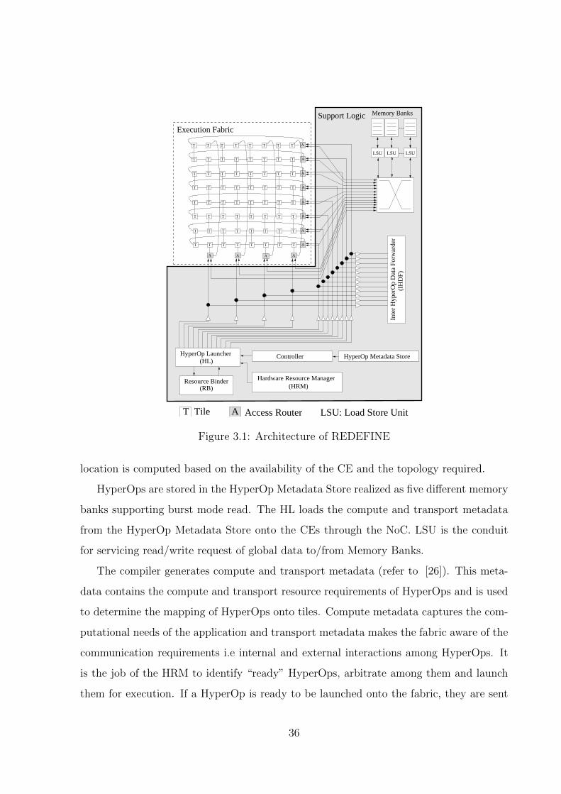
������
����
����
������
������
������
����
���
���
����
����
���
���T T T T T T T T
T T T T T T T T
T T T T T T T T
T T T T T T T T
T T T T T T T T
T T T T T T T T
T T T T T T T T
T T T T T T T T
LSULSULSU
Inte
r H
yper
Op
Dat
a Fo
rwar
der
(IH
DF)
Controller
Resource Binder(RB)
Hardware Resource Manager(HRM)
HyperOp Metadata Store
AT Tile Access Router LSU: Load Store Unit
A
A
A
A
A
A AA
...
...
Memory Banks
Execution Fabric
Support Logic
A
A
A
A
HyperOp Launcher(HL)
Figure 3.1: Architecture of REDEFINE
location is computed based on the availability of the CE and the topology required.
HyperOps are stored in the HyperOp Metadata Store realized as five different memory
banks supporting burst mode read. The HL loads the compute and transport metadata
from the HyperOp Metadata Store onto the CEs through the NoC. LSU is the conduit
for servicing read/write request of global data to/from Memory Banks.
The compiler generates compute and transport metadata (refer to [26]). This meta-
data contains the compute and transport resource requirements of HyperOps and is used
to determine the mapping of HyperOps onto tiles. Compute metadata captures the com-
putational needs of the application and transport metadata makes the fabric aware of the
communication requirements i.e internal and external interactions among HyperOps. It
is the job of the HRM to identify “ready” HyperOps, arbitrate among them and launch
them for execution. If a HyperOp is ready to be launched onto the fabric, they are sent
36
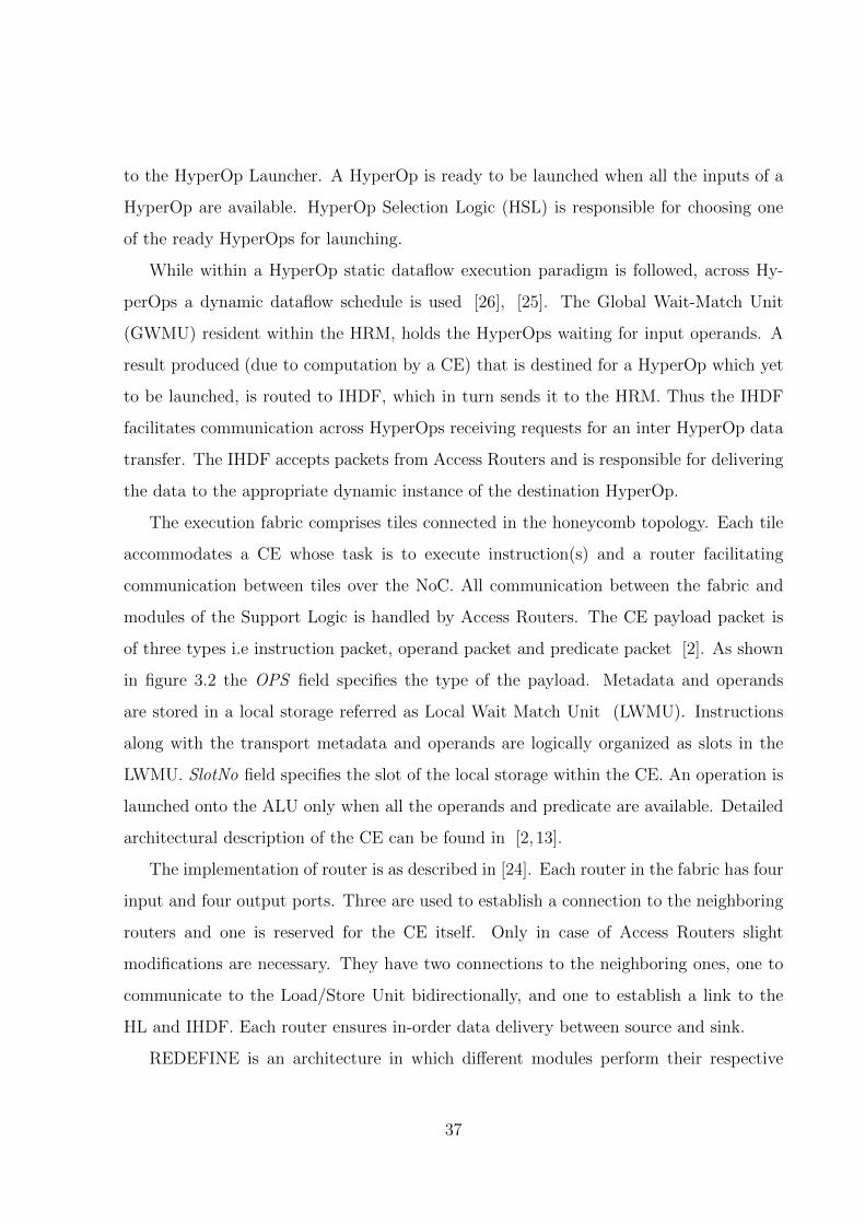
to the HyperOp Launcher. A HyperOp is ready to be launched when all the inputs of a
HyperOp are available. HyperOp Selection Logic (HSL) is responsible for choosing one
of the ready HyperOps for launching.
While within a HyperOp static dataflow execution paradigm is followed, across Hy-
perOps a dynamic dataflow schedule is used [26], [25]. The Global Wait-Match Unit
(GWMU) resident within the HRM, holds the HyperOps waiting for input operands. A
result produced (due to computation by a CE) that is destined for a HyperOp which yet
to be launched, is routed to IHDF, which in turn sends it to the HRM. Thus the IHDF
facilitates communication across HyperOps receiving requests for an inter HyperOp data
transfer. The IHDF accepts packets from Access Routers and is responsible for delivering
the data to the appropriate dynamic instance of the destination HyperOp.
The execution fabric comprises tiles connected in the honeycomb topology. Each tile
accommodates a CE whose task is to execute instruction(s) and a router facilitating
communication between tiles over the NoC. All communication between the fabric and
modules of the Support Logic is handled by Access Routers. The CE payload packet is
of three types i.e instruction packet, operand packet and predicate packet [2]. As shown
in figure 3.2 the OPS field specifies the type of the payload. Metadata and operands
are stored in a local storage referred as Local Wait Match Unit (LWMU). Instructions
along with the transport metadata and operands are logically organized as slots in the
LWMU. SlotNo field specifies the slot of the local storage within the CE. An operation is
launched onto the ALU only when all the operands and predicate are available. Detailed
architectural description of the CE can be found in [2, 13].
The implementation of router is as described in [24]. Each router in the fabric has four
input and four output ports. Three are used to establish a connection to the neighboring
routers and one is reserved for the CE itself. Only in case of Access Routers slight
modifications are necessary. They have two connections to the neighboring ones, one to
communicate to the Load/Store Unit bidirectionally, and one to establish a link to the
HL and IHDF. Each router ensures in-order data delivery between source and sink.
REDEFINE is an architecture in which different modules perform their respective
37
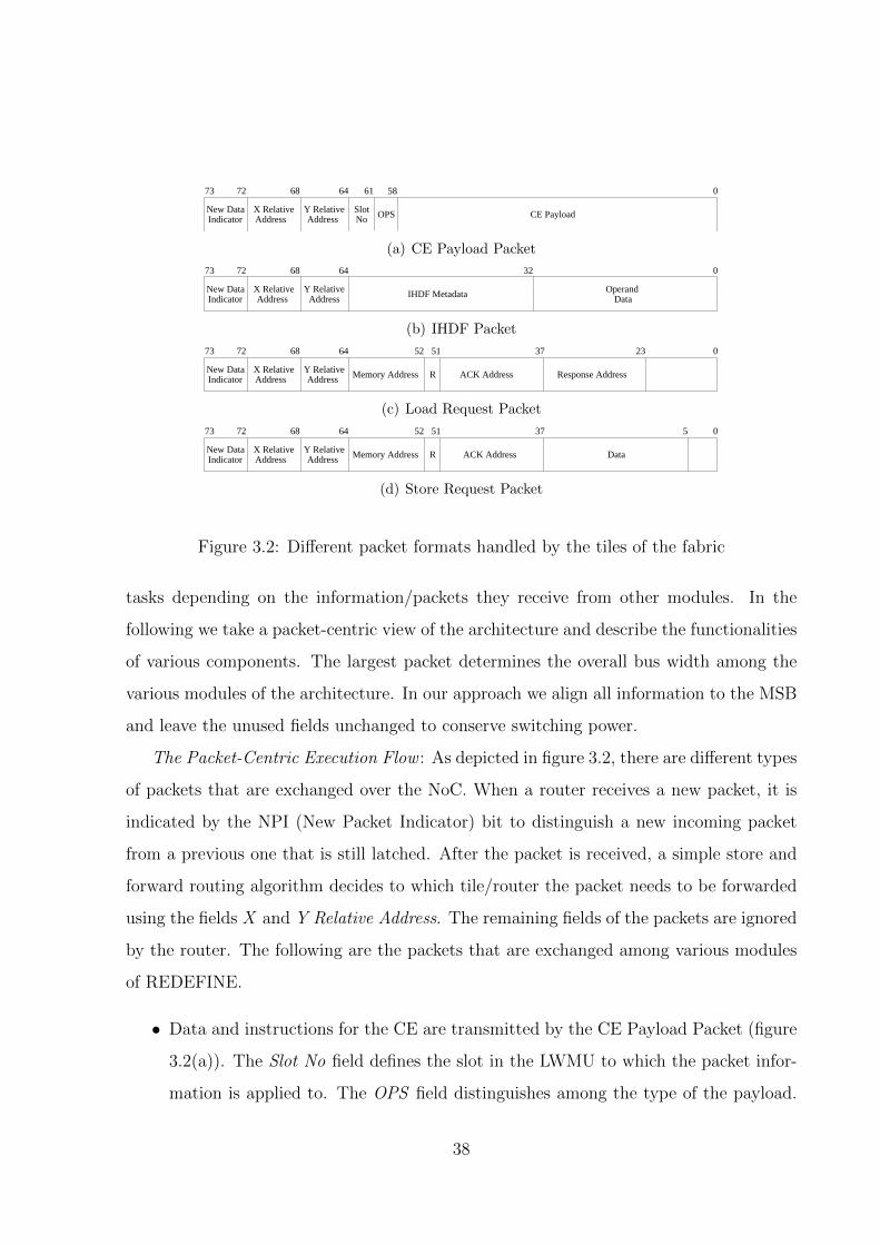
SlotNo
58 06164687273
OPS CE PayloadIndicator New Data X Relative
Address AddressY Relative
(a) CE Payload Packet
064687273 32
OperandDataIHDF MetadataIndicator
New Data X Relative Y RelativeAddress Address
(b) IHDF Packet
064687273
Memory Address R
52 51 37 23
Response AddressACK AddressIndicator X RelativeAddress Address
Y RelativeNew Data
(c) Load Request Packet
064687273
Memory Address R
52 51 37
Data
5
ACK AddressIndicator X RelativeAddress Address
Y RelativeNew Data
(d) Store Request Packet
Figure 3.2: Different packet formats handled by the tiles of the fabric
tasks depending on the information/packets they receive from other modules. In the
following we take a packet-centric view of the architecture and describe the functionalities
of various components. The largest packet determines the overall bus width among the
various modules of the architecture. In our approach we align all information to the MSB
and leave the unused fields unchanged to conserve switching power.
The Packet-Centric Execution Flow : As depicted in figure 3.2, there are different types
of packets that are exchanged over the NoC. When a router receives a new packet, it is
indicated by the NPI (New Packet Indicator) bit to distinguish a new incoming packet
from a previous one that is still latched. After the packet is received, a simple store and
forward routing algorithm decides to which tile/router the packet needs to be forwarded
using the fields X and Y Relative Address. The remaining fields of the packets are ignored
by the router. The following are the packets that are exchanged among various modules
of REDEFINE.
• Data and instructions for the CE are transmitted by the CE Payload Packet (figure
3.2(a)). The Slot No field defines the slot in the LWMU to which the packet infor-
mation is applied to. The OPS field distinguishes among the type of the payload.
38
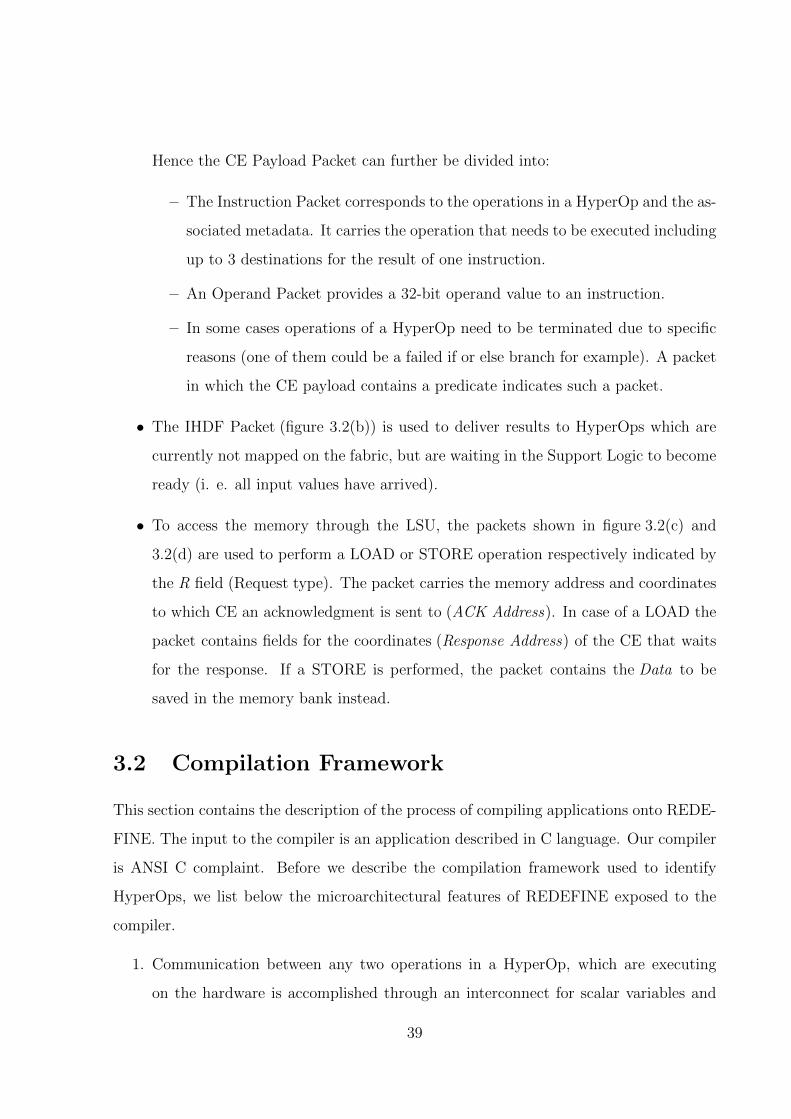
Hence the CE Payload Packet can further be divided into:
– The Instruction Packet corresponds to the operations in a HyperOp and the as-
sociated metadata. It carries the operation that needs to be executed including
up to 3 destinations for the result of one instruction.
– An Operand Packet provides a 32-bit operand value to an instruction.
– In some cases operations of a HyperOp need to be terminated due to specific
reasons (one of them could be a failed if or else branch for example). A packet
in which the CE payload contains a predicate indicates such a packet.
• The IHDF Packet (figure 3.2(b)) is used to deliver results to HyperOps which are
currently not mapped on the fabric, but are waiting in the Support Logic to become
ready (i. e. all input values have arrived).
• To access the memory through the LSU, the packets shown in figure 3.2(c) and
3.2(d) are used to perform a LOAD or STORE operation respectively indicated by
the R field (Request type). The packet carries the memory address and coordinates
to which CE an acknowledgment is sent to (ACK Address). In case of a LOAD the
packet contains fields for the coordinates (Response Address) of the CE that waits
for the response. If a STORE is performed, the packet contains the Data to be
saved in the memory bank instead.
3.2 Compilation Framework
This section contains the description of the process of compiling applications onto REDE-
FINE. The input to the compiler is an application described in C language. Our compiler
is ANSI C complaint. Before we describe the compilation framework used to identify
HyperOps, we list below the microarchitectural features of REDEFINE exposed to the
compiler.
1. Communication between any two operations in a HyperOp, which are executing
on the hardware is accomplished through an interconnect for scalar variables and
39
through memory for vector variables. (There is no central register file which is seen
by the compiler. The use of the interconnect enables direct communication of the
result and avoids the overhead of accessing the register file for a read or write.)
2. The interconnect follows a Honeycomb topology. Details of this topology are pro-
vided in [23].
3. All CEs are homogeneous. Each CE is capable of executing a set of arithmetic,
logic, compare and memory access operations. Apart from these operations, few
special operations are used to transfer data directly to other CEs.
4. In order delivery of data is guaranteed between each pair of communicating Hyper-
Ops that constitute a Custom Instruction.
The compilation process is divided into various phases:
• Phase I - Formation of Data Flow Graph (DFG): Application synthesis in
REDEFINE follows a data driven execution paradigm. The first phase transforms
the application into a dataflow graph (DFG) and performs several optimizations to
reduce the overhead of data transfer.
• Phase II - HyperOp formation: The basic entity in our paradigm is a HyperOp.
This phase divides the application into several HyperOps.
• Phase III - Tag generation: In our execution paradigm multiple HyperOp in-
stances can be active on the fabric simultaneously. To distinguish these HyperOps
we generate tags (similar to tags in dynamic dataflow [27]) at runtime by the hard-
ware. The necessary information required for the generation of the tags is identified
in this phase. To reduce the overhead of tag generation we generate tags only for
inputs and outputs of HyperOp. The data tokens within a HyperOp do not contain
a tag.
• Phase IV - Mapping HyperOps: This phase of compilation is aware of the
interconnect topology between the tiles of the reconfigurable fabric. The process
40
of Metadata generation involves identifying HyperOp partitions called p-HyperOps,
such that all operations in a p-HyperOp can be assigned to a single CE. These
p-HyperOps are mapped onto multiple CEs in the reconfigurable fabric based on
communication patterns between them.
• Phase V - Formation of Custom Instructions: This step identifies HyperOps
that can be aggregated into Custom Instructions. Custom Instructions are necessary
to reduce the overhead of inter HyperOp communication. Unlike HyperOps, Custom
Instructions need not be acyclic. We assume special hardware support to execute a
Custom Instruction.
3.3 Chapter Summary
In this chapter a laconic overview of REDEFINE, a CGRA has been presented. We
described both the microarchitecture and compiler support required for the same. The
microarchitecture comprises a reconfigurable fabric and necessary support logic to execute
the applications. The reconfigurable fabric is an interconnection of tiles in honeycomb
topology where each tile consists of a data driven Compute Element and a router. We
obviate the overheads of central register file by providing local storage at each Compute
Element and by delivering the data to the destination directly. We presented a compiler
for REDEFINE to realize the application described in a High Level Language (for ex: C)
onto the reconfigurable fabric. The compiler aggregates basic blocks to form larger acyclic
code blocks called HyperOps. Execution of HyperOps in REDEFINE follows a dynamic
dataflow schedule.
41
Chapter 4
Domain characterization of
REDEFINE in the context of NLA
An application written in a high level language ‘C’ is transformed into coarse grain oper-
ations called “HyperOps” [25] by RETARGET1, the compiler for REDEFINE. In order
to tailor REDEFINE for a specific application domain, compiler directives may be used
to force partitioning and assignment of HyperOps. We need to increase the execution
efficiency of parts of applications that are executed multiple number of times. In order
to address this, we suggest an improvement in REDEFINE. Computation structures are
provisioned once, and repeatedly used for the lifetime of the application. In other words,
computational structures are made persistent for the lifetime of HyperOps2. We provide
an implementation of the suggested improvements in this work. We provide the support
needed to efficiently execute core computations of the NLA domains. Core computations
are the computations that get statistically often executed in multiple applications of an
application domain. We architect specialized hardware to efficiently execute these com-
putations and enhance the CEs with this domain specific hardware. Further, domain
specific Custom Function Units (CFUs), which are micro architectural hardware assists
1RETARGET uses the LLVM [28] front end and generates HyperOps containing basic operations
defined by the virtual ISA2By lifetime of a HyperOp, we mean all its dynamic instances.
42
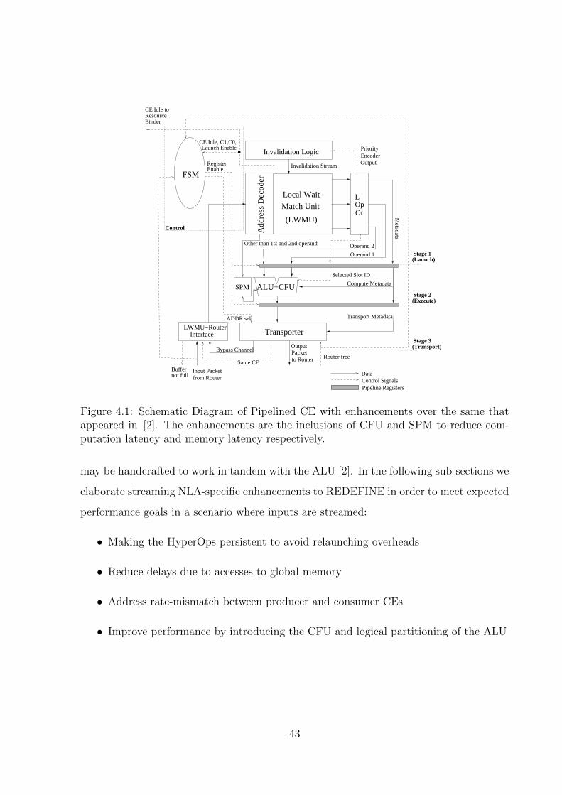
Invalidation Logic
OpL
Or
Invalidation Stream
FSM
OutputEncoderPriority
Transporter
OutputPacketto RouterSame CE
Bypass Channel
Input Packet from Router
Buffernot full
LWMU−RouterInterface
DataControl Signals
ADDR sel
Router free
Transport Metadata
Compute Metadata
Pipeline Registers
Control
Operand 1
Operand 2
Metadata
CE Idle toResourceBinder
CE Idle, C1,C0,Launch Enable
Add
ress
Dec
oder
(LWMU)
Match Unit
Local Wait
RegisterEnable
SPM
Other than 1st and 2nd operand
Selected Slot ID
Stage 1(Launch)
(Execute)Stage 2
Stage 3(Transport)
ALU+CFU
Figure 4.1: Schematic Diagram of Pipelined CE with enhancements over the same thatappeared in [2]. The enhancements are the inclusions of CFU and SPM to reduce com-putation latency and memory latency respectively.
may be handcrafted to work in tandem with the ALU [2]. In the following sub-sections we
elaborate streaming NLA-specific enhancements to REDEFINE in order to meet expected
performance goals in a scenario where inputs are streamed:
• Making the HyperOps persistent to avoid relaunching overheads
• Reduce delays due to accesses to global memory
• Address rate-mismatch between producer and consumer CEs
• Improve performance by introducing the CFU and logical partitioning of the ALU
43
4.1 Support for Persistent HyperOps and
Custom Instruction Pipeline
In order to meet very high throughput requirements of streaming applications relaunching
of HyperOps which get repeatedly executed, must be avoided. We build the capability
in the CEs to repeatedly perform the same set of operations. We rely on the support
provided by the compiler as reported in [13] for this enhancement.
To make HyperOps persistent, its instructions need to be repeatedly executed several
times. Therefore we introduce a new packet type for the CE Payload (refer to figure
3.2(a)). It contains a 16 bit value as counter representing the number of loop iterations
for which the instructions of one particular CE are valid. If all instructions of the CE
have been launched, the counter is decremented and the launch bits are reset. This
process repeats till the counter reaches a value of zero. Then the CE is declared as
idle representing that CE is ready to accept a new pHyperOp from the HL.3 In case
of streaming applications, HyperOps are made persistent throughout the lifetime of the
application by loading the counter with a value of zero. We further make improvements
by delivering loop invariant data only once for the lifetime of a loop.
Overheads incurred due to routing the results (produced by one HyperOp meant for an-
other HyperOp already resident on the fabric) through the Support Logic can be avoided,
by supporting channels of communication between the producing and consuming Hyper-
Ops.
Due to the Custom Instructions and the necessity of pipelines among them, in-order
delivery must be ensured. The routers send the packets to respective destinations ports
in the same order they have been received. Although packets are routed by a simple
forward-and-store routing algorithm, the order can be changed by the Virtual Channel
3In case Custom Instruction pipelines are not established, even with persistent HyperOps, inter-
HyperOp communications will be routed through the Support Logic. However in our case, RETARGET
specifies these inter-HyperOp communications and the necessary enhancements have been made to the
NoC. Hence we do not discuss the enhancements needed in the Support Logic for inter-HyperOp com-
munications.
44
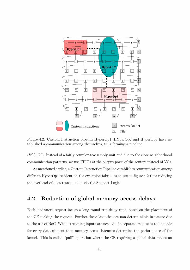
Custom Instructions
������
����
����
������������
������������
������������
����
���
���
����
����
���
���
����
T T T T T T T T
T T T T T T T T
T T T T T T T T
T T T T T T T T
T T T T T T T T
T T T T T T T T
T T T T T T T T
T T T T T T T T
T
A Access Router
Tile
A
A
A
A
A
A
A AAA
A
A
HyperOp1
HyperOp2
HyperOp3
Figure 4.2: Custom Instruction pipeline:HyperOp1, HYperOp2 and HyperOp3 have es-tablished a communication among themselves, thus forming a pipeline
(VC) [29]. Instead of a fairly complex reassembly unit and due to the close neighborhood
communication patterns, we use FIFOs at the output ports of the routers instead of VCs.
As mentioned earlier, a Custom Instruction Pipeline establishes communication among
different HyperOps resident on the execution fabric, as shown in figure 4.2 thus reducing
the overhead of data transmission via the Support Logic.
4.2 Reduction of global memory access delays
Each load/store request incurs a long round trip delay time, based on the placement of
the CE making the request. Further these latencies are non-deterministic in nature due
to the use of NoC. When streaming inputs are needed, if a separate request is to be made
for every data element then memory access latencies determine the performance of the
kernel. This is called “pull” operation where the CE requiring a global data makes an
45
explicit load request to the global memory. This delay introduced by this pull model gets
multiplied in case of streaming data - for every global load operation, the CE has to make
an explicit load request and wait for the global data. There are several ways of decreasing
this overhead. One mechanism is to enable the CE (to which streaming data is to be
loaded) to make one explicit request to the global memory; thereupon the global memory
streams the global data (without waiting for further load requests). In other words, a
“push” model, would require the global memory to “volunteer“ load of global data to
CEs. Another enhancement to reduce overheads due to global loads is to distribute and
pre-load the global data to CEs, provided CEs have local storage. Having local storage
will however not overcome the delay associated with indirect references. This delay can be
abated partially if the local memory has an associated logic to resolve indirect references
as part of the address calculation. The Scratch-Pad Memory (SPM) serves as the local
memory within each CE and Scratch-Pad Memory Controller (SPMC) has the additional
logic for indirect address calculation.
4.3 Flow-Control
In REDEFINE, rate mismatch between a producer and a consumer could arise due to
the use of NoC for communication of data. This is addressed by enforcing the consumer
to request the producer for data, once the consumer completes execution of one iteration
of operations assigned to it. In other words, intra and inter HyperOp communication for
propagating data, results in ”chaining“ of several producers and consumers. This requires
special logic in each CE, so as not to overwrite previously produced data. The scheme
followed here is similar to the principal that is used in case of wavefront arrays [5]. In
the wavefront architecture, the information transfer is by mutual convenience between
a PE and its immediate neighbors. In essence, wavefront processing promotes data-
driven computation. As REDEFINE conforms to the data-flow paradigm, the presence
of wavefront array features in the flow-control scheme is very logical.
46
4.4 Performance improvement - Introduction of CFU
Streaming applications require to speed-up certain critical operations in order to maintain
throughput. To speedup these operations we introduce a CFU in the CE. Such a CFU is
a customized unit for a specific application/domain. For example, most of the NLA ap-
plications require multiply-accumulate operations. These applications can execute much
faster, if a multiply-accumulate CFU is provided in the CE. In this section, we describe
the details of the enhancements required to support such CFUs. We provide flexibility in
choosing a CFU by allowing multiple input and multiple output CFUs.
To incorporate this CFU into the existing hardware infrastructure, we have introduced
extra operand types. These new operand types specify that the operands are meant for
the CFU. The SlotNo field (refer figure 3.2(a)) specifies the input number of the CFU.
Hence the number of inputs is limited by the number of bits assigned to the SlotNo field.
In normal operations same result is delivered to different destinations, as indicated by
the destination field. In case of CFU, different results are processed in the Transporter
in consecutive clock cycles to form result packets which are then sent to their respective
destinations via the NoC. The number of outputs of a CFU is limited by the number of
destination fields available in the instruction.
In the context of NLA kernels, the handcrafted CFUs perform core computations
required for matrix-vector multiplication i.e MAC, division, prime computations for QRD.
The structure of the CE reported in [13], with the modifications is shown in figure 4.1.
The ALU shown in this figure is capable of performing all instructions from the Virtual
ISA [13]. In case the ALU is not pipelined then it is obvious that the throughput of
this ALU is determined by the highest latency to perform one operation. We go for a
pipelined ALU and the operations have been categorized as either unit-cycle or multi-cycle
operations. If the CE has to satisfy the throughput requirements in case of streaming
inputs, then the ALU has to process both unit-cycle and multi-cycle operations. This
would result in pipeline bubbles, reducing the throughput. In order to overcome this we
logically partition the ALU into two units - one that performs unit cycle operations and
the other that performs multicycle operations. This has the added advantage that both
47
kinds of operations in the ALU can be relinquished, thereby reducing the contribution
to area occupied by the ALU. In our work along with direct solver we also realize sparse
matrix solver on REDEFINE. It is to be noted that core computations for both the direct
and iterative or sparse solvers use the same CFU, but they differ in their NoC usage.
Systolic algorithms are realized on REDEFINE by appropriate flow control i.e ”chaining“
the CEs.
4.5 Need for algorithm-aware compilation framework
In this section, we explore the need for algorithm-aware compilation framework. Data-
flow graphs compiled from the HLL descriptions of the applications contain sets of com-
putational nodes. Without using CFU, facilitating executions of compound instructions
composed of several such nodes, we cannot reduce the number of computational nodes
of a data-flow graph. So, preferred scenario is when the the number of cycles taken as
launch overhead is very less in comparison to the number of cycles spent on computa-
tions. Since the time taken for execution of a given set of instructions is fixed, smaller
launch overhead will result in improvement in overall performance. In stead of normal
multiplication when we go for block multiplication bigger HyperOps are formed. It has
been observed that the rate of increase in launch overhead with increasing HyperOp size
is less than the rate of increase in cycles spent on computations. Hence, overall launch
overhead (and inter HyperOp communication) of the application is reduced if bigger Hy-
perOps or bigger inner loops are formed from the application data-flow graph. We present
performance of a 18× 18 matrix multiplication in table 4.1 with various HyperOp size to
illustrate the above point. The numbers representing the cycle-counts are generated from
REDEFINE Simulator using general compilation technique. Using Block-multiplication
approach with Block size of 3 × 3 we can have a speed-up of almost 4× in comparison
to the first two instances of multiplications where HyperOp sizes are smaller. The loop
invariant code motion being active, the loading of a chunk of loop-invariant data can be
done ahead of entering the loops. As there is a limitation on the number of inputs per
HyperOp, the basic blocks are compelled to be broken into several HyperOps. Though
48
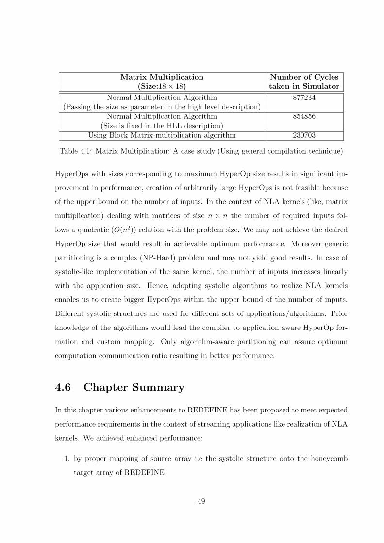
Matrix Multiplication Number of Cycles(Size:18× 18) taken in Simulator
Normal Multiplication Algorithm 877234(Passing the size as parameter in the high level description)
Normal Multiplication Algorithm 854856(Size is fixed in the HLL description)
Using Block Matrix-multiplication algorithm 230703
Table 4.1: Matrix Multiplication: A case study (Using general compilation technique)
HyperOps with sizes corresponding to maximum HyperOp size results in significant im-
provement in performance, creation of arbitrarily large HyperOps is not feasible because
of the upper bound on the number of inputs. In the context of NLA kernels (like, matrix
multiplication) dealing with matrices of size n × n the number of required inputs fol-
lows a quadratic (O(n2)) relation with the problem size. We may not achieve the desired
HyperOp size that would result in achievable optimum performance. Moreover generic
partitioning is a complex (NP-Hard) problem and may not yield good results. In case of
systolic-like implementation of the same kernel, the number of inputs increases linearly
with the application size. Hence, adopting systolic algorithms to realize NLA kernels
enables us to create bigger HyperOps within the upper bound of the number of inputs.
Different systolic structures are used for different sets of applications/algorithms. Prior
knowledge of the algorithms would lead the compiler to application aware HyperOp for-
mation and custom mapping. Only algorithm-aware partitioning can assure optimum
computation communication ratio resulting in better performance.
4.6 Chapter Summary
In this chapter various enhancements to REDEFINE has been proposed to meet expected
performance requirements in the context of streaming applications like realization of NLA
kernels. We achieved enhanced performance:
1. by proper mapping of source array i.e the systolic structure onto the honeycomb
target array of REDEFINE
49
2. by providing support needed to execute core computations of QRD i.e by introducing
customized CFUs addressing the computational needs of the NLA domain
3. by implementing push model for memory transaction for streaming applications like
Numerical Linear Algebra (NLA) kernels
4. by realizing proper flow control scheme (by philosophy analogous to that of wave-
front arrays) for consistent data-arrival
We further investigate the need for algorithm aware compilation framework that assures
better performance.
50
Chapter 5
Realization of Systolic Algorithms
on REDEFINE
In this chapter we discuss the details of the realization of two kinds of NLA kernels. We
target Modified Faddeev’s Algorithm (MFA) as a potential direct solver. We bring about
a proposition to realize MFA on REDEFINE, a coarse grained reconfigurable architec-
ture. We compare the performance numbers with that of a GPP solution to show that
REDEFINE performs several times faster than traditional GPPs. Further we channelize
our interest to QR Decomposition (QRD) to be the next NLA kernel as it ensures better
stability than LU and other decompositions. As in the context of MFA we already show
the performance enhancement in REDEFINE over GPP, we use QRD as a case study to
explore the design space of the solution on the proposed reconfigurable platform i.e REDE-
FINE. We also investigate the architectural details of the Custom Functional Units (CFU)
for these NLA kernels. Further, we report the synthesis results of CEs accommodating
those CFUs serving the needs for core computations.
5.1 Realization of Faddeev’s algorithm on REDEFINE
This section throws light on the methodology used to realize Faddeevs Algorithm on
REDEFINE. The exhaustive work has been reported in [9]. Excerpts of the paper are
51
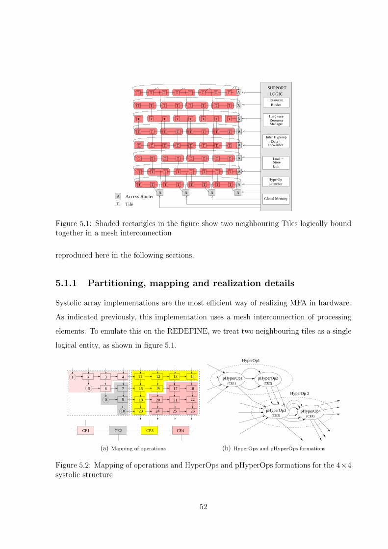
����
������
������
��������
��������
��������
��
����
T T T T T T T T
T T T T T T T T
T T T T T T T T
T T T T T T T T
T T T T T T T T
T T T T T T T T
T T T T T T T T
T T T T T T T T
T
A Access Router
Tile
SUPPORT
LOGIC
A
A
A
A
A
A
A
A
AA A A
BinderResource
HyperOpLauncher
Unit
Load −Store
ForwarderData
Inter Hyperop
Hardware Resource Manager
Global Memory
Figure 5.1: Shaded rectangles in the figure show two neighbouring Tiles logically boundtogether in a mesh interconnection
reproduced here in the following sections.
5.1.1 Partitioning, mapping and realization details
Systolic array implementations are the most efficient way of realizing MFA in hardware.
As indicated previously, this implementation uses a mesh interconnection of processing
elements. To emulate this on the REDEFINE, we treat two neighbouring tiles as a single
logical entity, as shown in figure 5.1.
8
1 2 3 4
5 6 7
9
10
11 12 13 14
15 16 17 18
19 20 21 22
23 24 2625
CE1 CE2 CE3 CE4
(a) Mapping of operations
pHyperOp1(CE2)
pHyperOp2
pHyperOp3(CE3)
pHyperOp4(CE4)
HyperOp 2
HyperOp1
(CE1)
(b) HyperOps and pHyperOps formations
Figure 5.2: Mapping of operations and HyperOps and pHyperOps formations for the 4×4systolic structure
52
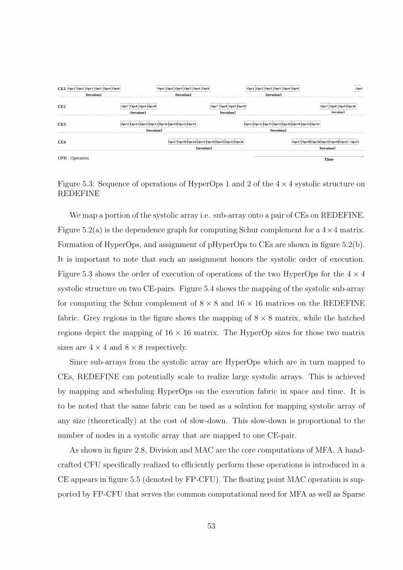
Opr1 Opr2 Opr3 Opr5 Opr4 Opr6
Opr16 Opr19 Opr23 Opr14Opr11 Opr12 Opr15 Opr13
Opr17 Opr20 Opr24 Opr18Opr21 Opr25 Opr22 Opr26 Opr22Opr25Opr18Opr21Opr24Opr20Opr17
Opr1 Opr2 Opr3 Opr5 Opr4 Opr6
Opr7 Opr8 Opr9 Opr10 Opr7 Opr8 Opr9 Opr10
Opr16 Opr19 Opr23 Opr14Opr11 Opr12 Opr15 Opr13
Opr7 Opr8 Opr9 Opr10
Opr1 Opr2 Opr3 Opr5 Opr4 Opr6CE1
CE2
CE3
CE4
Iteration3
Opr1
Time
Iteration1 Iteration2
Iteration3Iteration2Iteration1
Iteration1 Iteration2
Iteration1 Iteration2
OPR : Operation
Figure 5.3: Sequence of operations of HyperOps 1 and 2 of the 4× 4 systolic structure onREDEFINE
We map a portion of the systolic array i.e. sub-array onto a pair of CEs on REDEFINE.
Figure 5.2(a) is the dependence graph for computing Schur complement for a 4×4 matrix.
Formation of HyperOps, and assignment of pHyperOps to CEs are shown in figure 5.2(b).
It is important to note that such an assignment honors the systolic order of execution.
Figure 5.3 shows the order of execution of operations of the two HyperOps for the 4× 4
systolic structure on two CE-pairs. Figure 5.4 shows the mapping of the systolic sub-array
for computing the Schur complement of 8 × 8 and 16 × 16 matrices on the REDEFINE
fabric. Grey regions in the figure shows the mapping of 8 × 8 matrix, while the hatched
regions depict the mapping of 16 × 16 matrix. The HyperOp sizes for those two matrix
sizes are 4× 4 and 8× 8 respectively.
Since sub-arrays from the systolic array are HyperOps which are in turn mapped to
CEs, REDEFINE can potentially scale to realize large systolic arrays. This is achieved
by mapping and scheduling HyperOps on the execution fabric in space and time. It is
to be noted that the same fabric can be used as a solution for mapping systolic array of
any size (theoretically) at the cost of slow-down. This slow-down is proportional to the
number of nodes in a systolic array that are mapped to one CE-pair.
As shown in figure 2.8, Division and MAC are the core computations of MFA. A hand-
crafted CFU specifically realized to efficiently perform these operations is introduced in a
CE appears in figure 5.5 (denoted by FP-CFU). The floating point MAC operation is sup-
ported by FP-CFU that serves the common computational need for MFA as well as Sparse
53
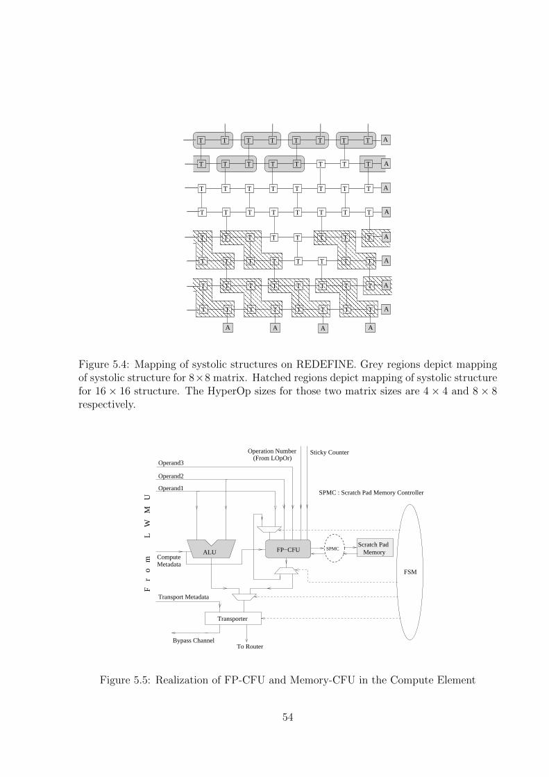
������������������������������������������������
������������������������������������������������
������������������������������������
������������������������������������
������������������������������������������������������
������������������������������������������������������
������������
������������
������������������������������������
������������������������������������
������������������������������������������������
������������������������������������������������
������������������������������������������������������
������������������������������������������������������
������������������������������������������������
������������������������������������������������
��������������������
��������������������
������
����
����
����
������
������
����
����
���
���
����
����
���
���T T T T T T T T
T T T T T T T T
T T T T T T T T
T T T T T T T T
T T T T T T T T
T T T T T T T T
T T T T T T T T
T T T T T T T T
A
A
A
A
A
A AA
A
A
A
A
Figure 5.4: Mapping of systolic structures on REDEFINE. Grey regions depict mappingof systolic structure for 8×8 matrix. Hatched regions depict mapping of systolic structurefor 16× 16 structure. The HyperOp sizes for those two matrix sizes are 4× 4 and 8× 8respectively.
Transporter
ALU
Bypass Channel
ComputeMetadata
Operand3
Operand2
Operand1
F
r o
m
L
W
M
U
Transport Metadata
FP−CFU SPMCMemory
FSM
To Router
SPMC : Scratch Pad Memory Controller
Sticky Counter
Scratch Pad
Operation Number(From LOpOr)
Figure 5.5: Realization of FP-CFU and Memory-CFU in the Compute Element
54
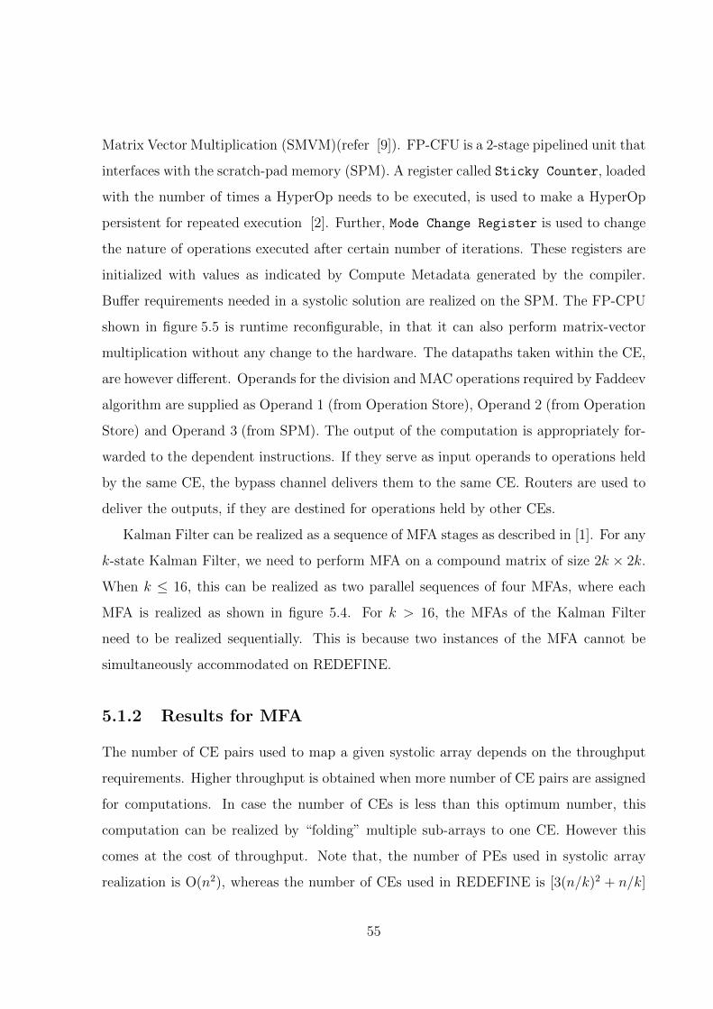
Matrix Vector Multiplication (SMVM)(refer [9]). FP-CFU is a 2-stage pipelined unit that
interfaces with the scratch-pad memory (SPM). A register called Sticky Counter, loaded
with the number of times a HyperOp needs to be executed, is used to make a HyperOp
persistent for repeated execution [2]. Further, Mode Change Register is used to change
the nature of operations executed after certain number of iterations. These registers are
initialized with values as indicated by Compute Metadata generated by the compiler.
Buffer requirements needed in a systolic solution are realized on the SPM. The FP-CPU
shown in figure 5.5 is runtime reconfigurable, in that it can also perform matrix-vector
multiplication without any change to the hardware. The datapaths taken within the CE,
are however different. Operands for the division and MAC operations required by Faddeev
algorithm are supplied as Operand 1 (from Operation Store), Operand 2 (from Operation
Store) and Operand 3 (from SPM). The output of the computation is appropriately for-
warded to the dependent instructions. If they serve as input operands to operations held
by the same CE, the bypass channel delivers them to the same CE. Routers are used to
deliver the outputs, if they are destined for operations held by other CEs.
Kalman Filter can be realized as a sequence of MFA stages as described in [1]. For any
k-state Kalman Filter, we need to perform MFA on a compound matrix of size 2k × 2k.
When k ≤ 16, this can be realized as two parallel sequences of four MFAs, where each
MFA is realized as shown in figure 5.4. For k > 16, the MFAs of the Kalman Filter
need to be realized sequentially. This is because two instances of the MFA cannot be
simultaneously accommodated on REDEFINE.
5.1.2 Results for MFA
The number of CE pairs used to map a given systolic array depends on the throughput
requirements. Higher throughput is obtained when more number of CE pairs are assigned
for computations. In case the number of CEs is less than this optimum number, this
computation can be realized by “folding” multiple sub-arrays to one CE. However this
comes at the cost of throughput. Note that, the number of PEs used in systolic array
realization is O(n2), whereas the number of CEs used in REDEFINE is [3(n/k)2 + n/k]
55
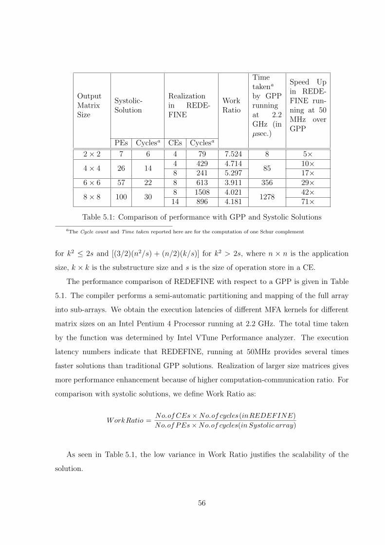
OutputMatrixSize
Systolic-Solution
Realizationin REDE-FINE
WorkRatio
Timetakena
by GPPrunningat 2.2GHz (inµsec.)
Speed Upin REDE-FINE run-ning at 50MHz overGPP
PEs Cyclesa CEs Cyclesa
2× 2 7 6 4 79 7.524 8 5×
4× 4 26 144 429 4.714
8510×
8 241 5.297 17×6× 6 57 22 8 613 3.911 356 29×
8× 8 100 308 1508 4.021
127842×
14 896 4.181 71×
Table 5.1: Comparison of performance with GPP and Systolic Solutions
aThe Cycle count and Time taken reported here are for the computation of one Schur complement
for k2 ≤ 2s and [(3/2)(n2/s) + (n/2)(k/s)] for k2 > 2s, where n × n is the application
size, k × k is the substructure size and s is the size of operation store in a CE.
The performance comparison of REDEFINE with respect to a GPP is given in Table
5.1. The compiler performs a semi-automatic partitioning and mapping of the full array
into sub-arrays. We obtain the execution latencies of different MFA kernels for different
matrix sizes on an Intel Pentium 4 Processor running at 2.2 GHz. The total time taken
by the function was determined by Intel VTune Performance analyzer. The execution
latency numbers indicate that REDEFINE, running at 50MHz provides several times
faster solutions than traditional GPP solutions. Realization of larger size matrices gives
more performance enhancement because of higher computation-communication ratio. For
comparison with systolic solutions, we define Work Ratio as:
WorkRatio =No.of CEs×No.of cycles(inREDEFINE)
No.of PEs×No.of cycles(in Systolic array)
As seen in Table 5.1, the low variance in Work Ratio justifies the scalability of the
solution.
56
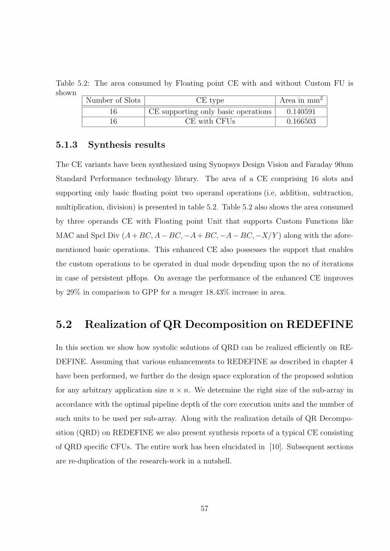
Table 5.2: The area consumed by Floating point CE with and without Custom FU isshown
Number of Slots CE type Area in mm2
16 CE supporting only basic operations 0.14059116 CE with CFUs 0.166503
5.1.3 Synthesis results
The CE variants have been synthesized using Synopsys Design Vision and Faraday 90nm
Standard Performance technology library. The area of a CE comprising 16 slots and
supporting only basic floating point two operand operations (i.e, addition, subtraction,
multiplication, division) is presented in table 5.2. Table 5.2 also shows the area consumed
by three operands CE with Floating point Unit that supports Custom Functions like
MAC and Spcl Div (A+BC,A−BC,−A+BC,−A−BC,−X/Y ) along with the afore-
mentioned basic operations. This enhanced CE also possesses the support that enables
the custom operations to be operated in dual mode depending upon the no of iterations
in case of persistent pHops. On average the performance of the enhanced CE improves
by 29% in comparison to GPP for a meager 18.43% increase in area.
5.2 Realization of QR Decomposition on REDEFINE
In this section we show how systolic solutions of QRD can be realized efficiently on RE-
DEFINE. Assuming that various enhancements to REDEFINE as described in chapter 4
have been performed, we further do the design space exploration of the proposed solution
for any arbitrary application size n× n. We determine the right size of the sub-array in
accordance with the optimal pipeline depth of the core execution units and the number of
such units to be used per sub-array. Along with the realization details of QR Decompo-
sition (QRD) on REDEFINE we also present synthesis reports of a typical CE consisting
of QRD specific CFUs. The entire work has been elucidated in [10]. Subsequent sections
are re-duplication of the research-work in a nutshell.
57
5.2.1 Actualization Details
The execution core of REDEFINE comprises multiple CEs (refer figure 5.1). Schematic
diagram of a CE is shown in figure 4.1. Operations assigned to a CE, are stored in Local
Wait Match Unit (LWMU). An operation is ready for execution only when all its input
operands are received. It is to be noted that in a honeycomb topology, every node is a
degree 3 element.
For systolic realization of QRD, the desired lattice is a mesh interconnection of pro-
cessing elements. It is well known that systolic arrays are not scalable due to their rigid
hard-wired structures. In this chapter we leverage systolic solution for QRD and cast
them on REDEFINE. In general, systolic solutions are derived to exploit local commu-
nication between nodes in a systolic array. Toroidal honeycomb topology of REDEFINE
can be rendered to support a mesh like lattice structure by combining two neighbouring
Tiles as a single logical entity as shown in figure 5.1. Each shaded region in the figure
depicts a CE-pair.
We map a sub-array of the systolic array onto a pair of CEs on REDEFINE. Each
sub-array therefore represents a HyperOp. Depending on the size of the matrix being
solved, the systolic array (representing the solution) is divided into multiple HyperOps.
In turn each HyperOp is divided into pHyperOps; and each pHyperOp is assigned a
CE in the CE-pair. Figure 5.6(a) is the dependence graph for computing QRD of a
8 × 8 matrix. Formation of HyperOps, and assignment of pHyperOps to CEs are also
shown in figure 5.6(a) and figure 5.6(b) respectively. It is important to note that such
an assignment honors the systolic order of execution. The dashed lines in figure 5.6(a)
represents the scheduling hyperplanes. The computations follow the scheduling vector −→s ,
which is orthogonal to the hyperplanes. The flow of the hyperplanes depicts the order
of execution of operations of the HyperOps. This order obeys permissible linear schedule
conditions [5] by ensuring
• All the dependency arcs flow in the same direction across the hyperplanes i.e causal-
ity is enforced.
58
• The hyperplanes1 are not parallel with the projection vector i.e the nodes on an
equitemporal hyperplane are not projected to the same CE.
In REDEFINE, all the operations representing the systolic solution are realized in
terms of instructions which are executed efficiently in the hand-crafted CFU of the CE.
Instructions forming the HyperOp get executed repeatedly on the fabric as persistent
HyperOps [2] till the maximum number of iterations needed for the particular output
matrix size is reached. A 16 bit register maintains the iteration count [2]. In the systolic
realization of QRD, there is a set of diagonal elements that generate factors (C and S as
indicated in the figure 2.11) in every iteration and these factors are passed along the row.
Once these factors are generated, they can be re-used for evaluation of other instructions
of the same row. Storing of these factors in SPM, will reduce overhead compared to
the situation when they are stored in global memory. Similarly, the computed values
indicated by R in figure 2.11 (corresponding to intermediate values stored in the registers
of the systolic array) can also be stored in SPM, thus eliminating the overheads associated
with delivering the factor using the bypass channel (refer figure 4.1) for propagation of
R. Use of SPM for locally storing C, S and R potentially reduces communications. For
instructions representing diagonal computations intra-CE communication is not required.
If elements of same row are realized in different CEs then inter-CE communication is
required. In case of off-diagonal computations number of output propagations is reduced
from 4 (as shown in figure 2.11) to 1.
Wavefront Array processors [5] are the ASIC realizations of systolic arrays, with data-
flow execution semantics. Systolic scheduling in this case propagates as a wave. RE-
DEFINE is akin to realization of wavefront array schedules, since it follows data driven
paradigm both for execution of operations and communication of output data. How-
ever rate-mismatches arising in such a situation is overcome by “chaining” the producer-
consumer CEs. This mechanism is similar to the modular processing units of a Wavefront
Array.
Global memory is used to store the initial matrices. QRD realization to cater to
1In systolic realization hyperplanes contain nodes that can be potentially executed in parallel
59
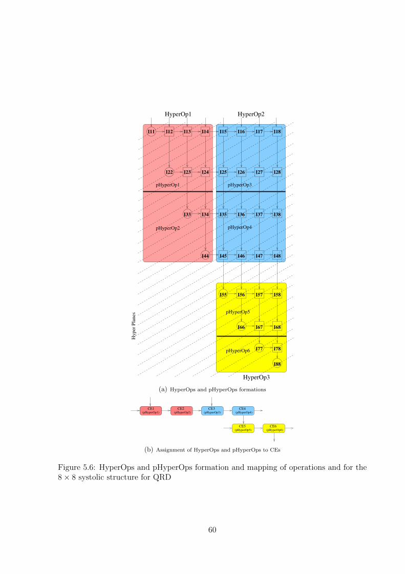
HyperOp3
pHyperOp1
pHyperOp2
pHyperOp3
pHyperOp4
pHyperOp5
pHyperOp6
HyperOp1 HyperOp2
Hy
per
Pla
nes
I11 I12 I13 I14 I15 I16 I17 I18
I22 I23 I24 I25 I26 I27 I28
I33 I34 I35 I36 I37 I38
I44 I45 I46 I47 I48
I55 I56 I57 I58
I66 I67 I68
I77 I78
I88
(a) HyperOps and pHyperOps formations
CE1(pHyperOp1)
CE2 CE3 CE4
CE5 CE6
(pHyperOp2) (pHyperOp3) (pHyperOp4)
(pHyperOp5) (pHyperOp6)
(b) Assignment of HyperOps and pHyperOps to CEs
Figure 5.6: HyperOps and pHyperOps formation and mapping of operations and for the8× 8 systolic structure for QRD
60
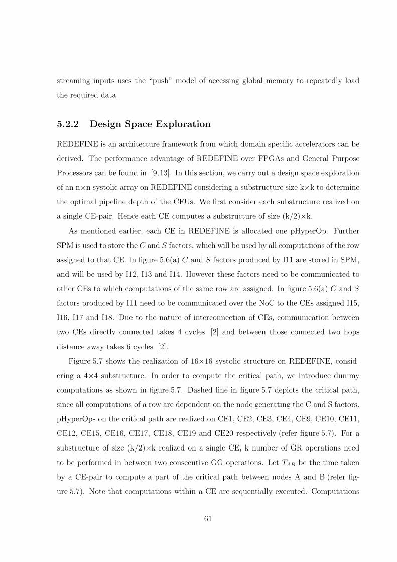
streaming inputs uses the “push” model of accessing global memory to repeatedly load
the required data.
5.2.2 Design Space Exploration
REDEFINE is an architecture framework from which domain specific accelerators can be
derived. The performance advantage of REDEFINE over FPGAs and General Purpose
Processors can be found in [9,13]. In this section, we carry out a design space exploration
of an n×n systolic array on REDEFINE considering a substructure size k×k to determine
the optimal pipeline depth of the CFUs. We first consider each substructure realized on
a single CE-pair. Hence each CE computes a substructure of size (k/2)×k.
As mentioned earlier, each CE in REDEFINE is allocated one pHyperOp. Further
SPM is used to store the C and S factors, which will be used by all computations of the row
assigned to that CE. In figure 5.6(a) C and S factors produced by I11 are stored in SPM,
and will be used by I12, I13 and I14. However these factors need to be communicated to
other CEs to which computations of the same row are assigned. In figure 5.6(a) C and S
factors produced by I11 need to be communicated over the NoC to the CEs assigned I15,
I16, I17 and I18. Due to the nature of interconnection of CEs, communication between
two CEs directly connected takes 4 cycles [2] and between those connected two hops
distance away takes 6 cycles [2].
Figure 5.7 shows the realization of 16×16 systolic structure on REDEFINE, consid-
ering a 4×4 substructure. In order to compute the critical path, we introduce dummy
computations as shown in figure 5.7. Dashed line in figure 5.7 depicts the critical path,
since all computations of a row are dependent on the node generating the C and S factors.
pHyperOps on the critical path are realized on CE1, CE2, CE3, CE4, CE9, CE10, CE11,
CE12, CE15, CE16, CE17, CE18, CE19 and CE20 respectively (refer figure 5.7). For a
substructure of size (k/2)×k realized on a single CE, k number of GR operations need
to be performed in between two consecutive GG operations. Let TAB be the time taken
by a CE-pair to compute a part of the critical path between nodes A and B (refer fig-
ure 5.7). Note that computations within a CE are sequentially executed. Computations
61
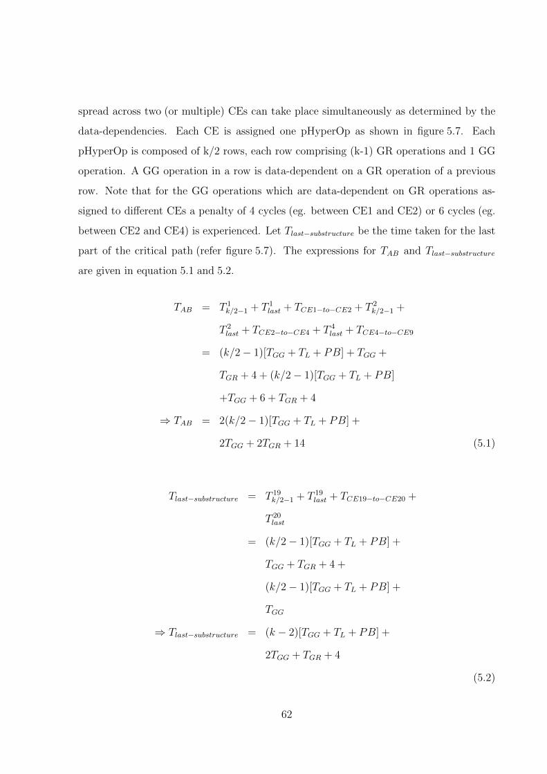
spread across two (or multiple) CEs can take place simultaneously as determined by the
data-dependencies. Each CE is assigned one pHyperOp as shown in figure 5.7. Each
pHyperOp is composed of k/2 rows, each row comprising (k-1) GR operations and 1 GG
operation. A GG operation in a row is data-dependent on a GR operation of a previous
row. Note that for the GG operations which are data-dependent on GR operations as-
signed to different CEs a penalty of 4 cycles (eg. between CE1 and CE2) or 6 cycles (eg.
between CE2 and CE4) is experienced. Let Tlast−substructure be the time taken for the last
part of the critical path (refer figure 5.7). The expressions for TAB and Tlast−substructure
are given in equation 5.1 and 5.2.
TAB = T 1k/2−1 + T 1
last + TCE1−to−CE2 + T 2k/2−1 +
T 2last + TCE2−to−CE4 + T 4
last + TCE4−to−CE9
= (k/2− 1)[TGG + TL + PB] + TGG +
TGR + 4 + (k/2− 1)[TGG + TL + PB]
+TGG + 6 + TGR + 4
⇒ TAB = 2(k/2− 1)[TGG + TL + PB] +
2TGG + 2TGR + 14 (5.1)
Tlast−substructure = T 19k/2−1 + T 19
last + TCE19−to−CE20 +
T 20last
= (k/2− 1)[TGG + TL + PB] +
TGG + TGR + 4 +
(k/2− 1)[TGG + TL + PB] +
TGG
⇒ Tlast−substructure = (k − 2)[TGG + TL + PB] +
2TGG + TGR + 4
(5.2)
62

where
T jk/2−1 = Cycles taken for computations of
(k/2− 1) rows realized in CEj
T jlast = Cycles taken for computations of last
row in CEj before the consumer CE
starts its computation
TCEi−to−CEj = Cycles taken for data delivery
from CEi to CEj
PB = Pipeline Bubbles
TGG = Cycles taken for one GG operation
TGR = Cycles taken for one GR operation
TL = Cycles taken for launching of all GR
operationsin between two consecutive
GG operations.
Once the factors C and S (refer figure 2.11) are generated, there is no data dependency
among the instructions of a row. However there is data dependency between an instruction
in a row and an instruction in the successor row (for eg.: instruction I12 and I22 in
figure 5.6). As depicted in figure 4.1, each CE has three stages, viz., Launch, Execute and
Transport. As a general case study if the Execute stages for GG and GR operations are
further realized as m1 and m2-stage units respectively, and an instruction which is data
dependent on another instruction allocated to the same CE (eg.: I12 and I22 in figure 5.6),
then the time difference between the two instructions entering the Execute stage is m2+2.
If k<(m2+2), then the number of pipeline bubbles experienced between computations
of these two instructions is (m2+2)-k. Pipeline is free of bubbles, if k>(m2+2). The
transporter transports only one packet at a time. Hence, an operation, eg. GG operation
resides for (m1+1) cycles in the execute stage. The GG operation takes m cycles for
63
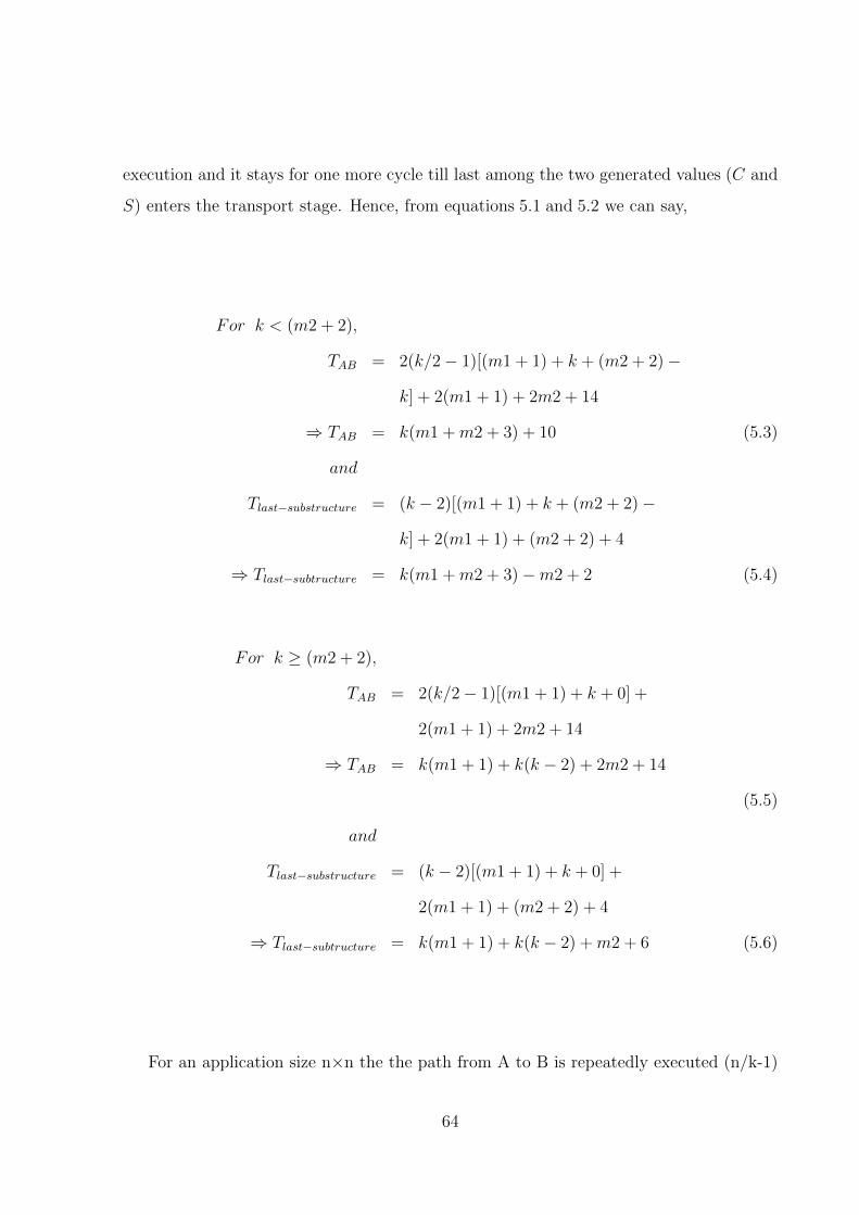
execution and it stays for one more cycle till last among the two generated values (C and
S) enters the transport stage. Hence, from equations 5.1 and 5.2 we can say,
For k < (m2 + 2),
TAB = 2(k/2− 1)[(m1 + 1) + k + (m2 + 2)−
k] + 2(m1 + 1) + 2m2 + 14
⇒ TAB = k(m1 +m2 + 3) + 10 (5.3)
and
Tlast−substructure = (k − 2)[(m1 + 1) + k + (m2 + 2)−
k] + 2(m1 + 1) + (m2 + 2) + 4
⇒ Tlast−subtructure = k(m1 +m2 + 3)−m2 + 2 (5.4)
For k ≥ (m2 + 2),
TAB = 2(k/2− 1)[(m1 + 1) + k + 0] +
2(m1 + 1) + 2m2 + 14
⇒ TAB = k(m1 + 1) + k(k − 2) + 2m2 + 14
(5.5)
and
Tlast−substructure = (k − 2)[(m1 + 1) + k + 0] +
2(m1 + 1) + (m2 + 2) + 4
⇒ Tlast−subtructure = k(m1 + 1) + k(k − 2) +m2 + 6 (5.6)
For an application size n×n the the path from A to B is repeatedly executed (n/k-1)
64
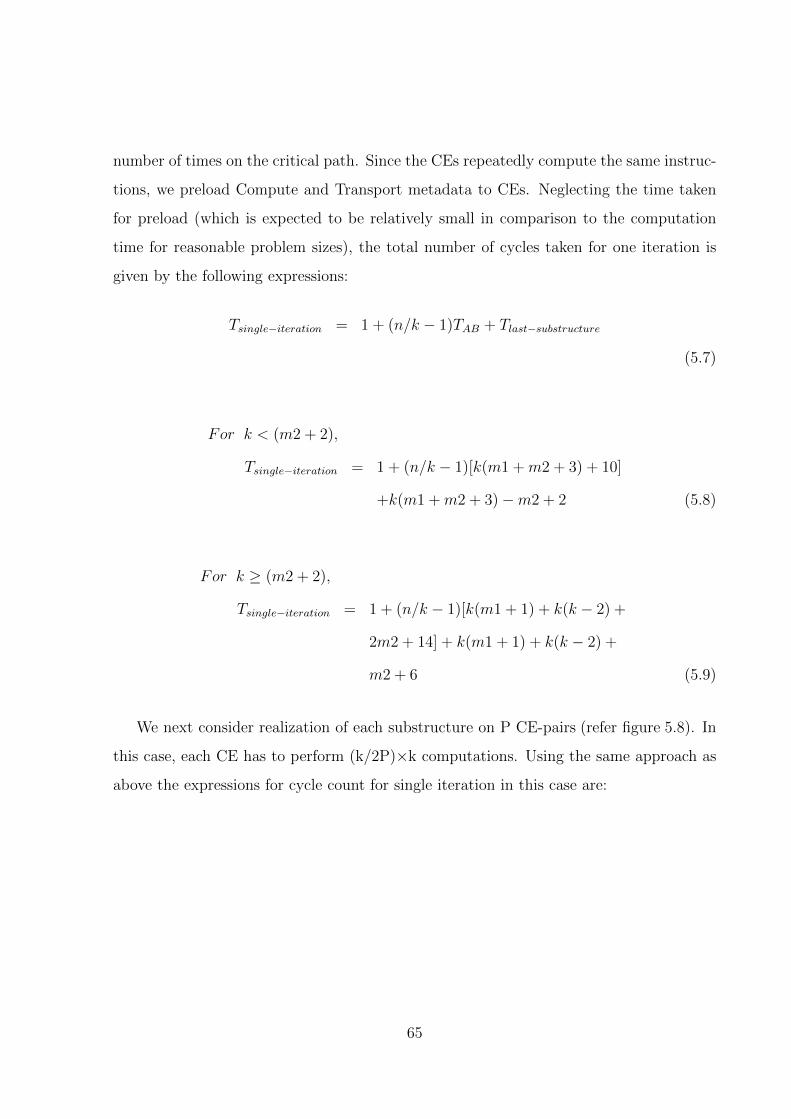
number of times on the critical path. Since the CEs repeatedly compute the same instruc-
tions, we preload Compute and Transport metadata to CEs. Neglecting the time taken
for preload (which is expected to be relatively small in comparison to the computation
time for reasonable problem sizes), the total number of cycles taken for one iteration is
given by the following expressions:
Tsingle−iteration = 1 + (n/k − 1)TAB + Tlast−substructure
(5.7)
For k < (m2 + 2),
Tsingle−iteration = 1 + (n/k − 1)[k(m1 +m2 + 3) + 10]
+k(m1 +m2 + 3)−m2 + 2 (5.8)
For k ≥ (m2 + 2),
Tsingle−iteration = 1 + (n/k − 1)[k(m1 + 1) + k(k − 2) +
2m2 + 14] + k(m1 + 1) + k(k − 2) +
m2 + 6 (5.9)
We next consider realization of each substructure on P CE-pairs (refer figure 5.8). In
this case, each CE has to perform (k/2P)×k computations. Using the same approach as
above the expressions for cycle count for single iteration in this case are:
65
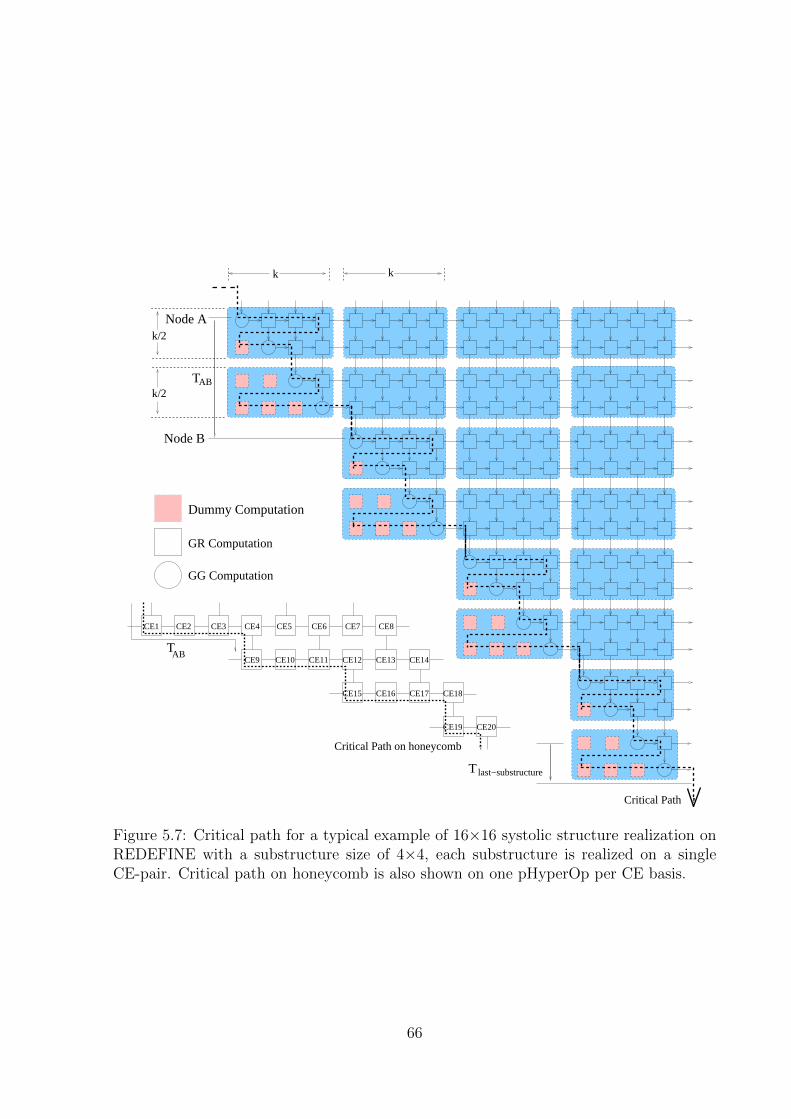
ABT
Node A
Node B
Dummy Computation
GG Computation
GR Computation
CE1 CE2
CE11 CE12 CE13
CE4CE3 CE5 CE6 CE7 CE8
CE9 CE10 CE14
CE15 CE16 CE17 CE18
CE19 CE20
last−substructureT
TAB
k k
k/2
k/2
Critical Path
Critical Path on honeycomb
Figure 5.7: Critical path for a typical example of 16×16 systolic structure realization onREDEFINE with a substructure size of 4×4, each substructure is realized on a singleCE-pair. Critical path on honeycomb is also shown on one pHyperOp per CE basis.
66
For k < (m2 + 2),
Tsingle−iteration = 1 + (n/k − 1)[k(m1 + 1) +
(m2 + 2)(k − 2P ) + (m2 + 4)(2P − 1) +m2 + 10]
+k(m1 + 1) + (m2 + 2)(k − 2P ) + (m2 + 4)(2P − 1)
(5.10)
For k ≥ (m2 + 2),
Tsingle−iteration = 1 + (n/k − 1)[k(m1 + 1) + k(k − 2P )
+(m2 + 4)(2P − 1) +m2 + 10] +
k(m1 + 1) + k(k − 2P ) + (m2 + 4)(2P − 1)
(5.11)
In order to complete the factorization of a given n×n matrix, n iterations need to
be performed. However, as mentioned earlier, in order to ensure correct execution on
REDEFINE, the producer and consumer CEs need to be “chained”. This is achieved
by the consumer CE sending an “acknowledgment” signal to the producer CE. Acknowl-
edgements are needed to address rate-mismatch between producer and consumer CEs.
As a consequence between two consecutive iterations a finite time gap as indicated by
Titeration−gap in figure 5.12 is experienced. From figure 5.12 the generic expression for total
n iterations of the critical path can be shown as
Tn−iterations = Tsingle−iteration + (n− 1)[Titeration−gap + Tlast−phOp] (5.12)
Titeration−gap = Tnon−overlap + Tack (5.13)
67
The expression for completely factorizing a n×n matrix is given by
For k < (m2 + 2),
Tn−iterations = 1 + (n/k − 1)[k(m1 + 1) +
(m2 + 2)(k − 2P ) + (m2 + 4)(2P − 1) +
m2 + 10] + k(m1 + 1) +
(m2 + 2)(k − 2P ) + (m2 + 4)
(2P − 1) + (n− 1)[4 + (m1 + 1)k/P +
(m2 + 2)(k/P − 2)− k/2P +
+2m2 + Tack] (5.14)
For k ≥ (m+ 2),
Tn−iterations = 1 + (n/k − 1)[k(m1 + 1) +
k(k − 2P ) + (m2 + 4)(2P − 1) +
m2 + 10] + k(m1 + 1) + k(k − 2P ) +
(m2 + 4)(2P − 1) + (n− 1)[4 +
(m1 + 1)k/P + k(k/P − 2)−
k/2P + 2m2 + Tack]
(5.15)
where Tack is the time taken for the acknowledgment to travel from consumer CE to
producer CE.
In the above, it is assumed that both GG and GR operations are executed in CFUs
of pipeline depth m. However in reality, they could be executed in two CFUs of different
pipeline depths i.e m1 and m2 respectively. Generally m1 is greater than m2 due to the
complexity of GG operations over GR operations. There is only one GG operation per
row and once one GG operation is done the next k number of GR operations before the
68
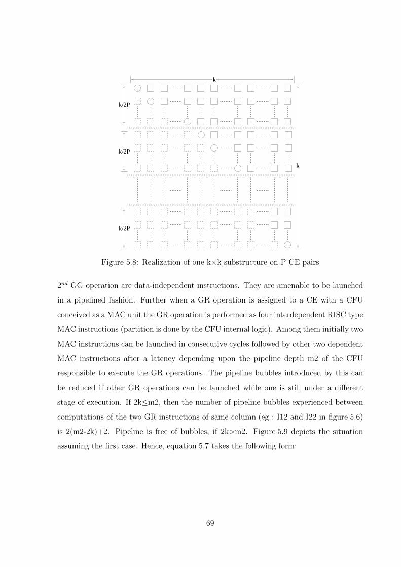
k/2P
k/2P
k/2P
k
k
Figure 5.8: Realization of one k×k substructure on P CE pairs
2nd GG operation are data-independent instructions. They are amenable to be launched
in a pipelined fashion. Further when a GR operation is assigned to a CE with a CFU
conceived as a MAC unit the GR operation is performed as four interdependent RISC type
MAC instructions (partition is done by the CFU internal logic). Among them initially two
MAC instructions can be launched in consecutive cycles followed by other two dependent
MAC instructions after a latency depending upon the pipeline depth m2 of the CFU
responsible to execute the GR operations. The pipeline bubbles introduced by this can
be reduced if other GR operations can be launched while one is still under a different
stage of execution. If 2k≤m2, then the number of pipeline bubbles experienced between
computations of the two GR instructions of same column (eg.: I12 and I22 in figure 5.6)
is 2(m2-2k)+2. Pipeline is free of bubbles, if 2k>m2. Figure 5.9 depicts the situation
assuming the first case. Hence, equation 5.7 takes the following form:
69
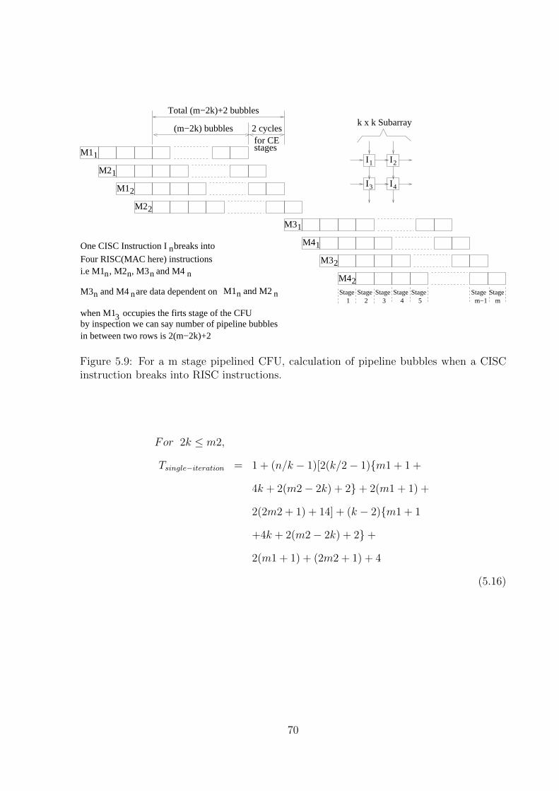
1M2
2M1
2M2
1M1
i.e M1 , M2 , M3 and M4n n n n
I2I1
I3 I4
2M4
1
1
2
M4
M3
M3
Stage1
Stage2
Stage3
Stage4
Stage5
Stagem−1
Stagem
n nM3 and M4 are data dependent on n nM1 and M2
k x k Subarray(m−2k) bubbles 2 cycles
for CEstages
Total (m−2k)+2 bubbles
by inspection we can say number of pipeline bubblesin between two rows is 2(m−2k)+2
Four RISC(MAC here) instructions
One CISC Instruction I breaks into
when M1 occupies the firts stage of the CFU 3
n
Figure 5.9: For a m stage pipelined CFU, calculation of pipeline bubbles when a CISCinstruction breaks into RISC instructions.
For 2k ≤ m2,
Tsingle−iteration = 1 + (n/k − 1)[2(k/2− 1){m1 + 1 +
4k + 2(m2− 2k) + 2}+ 2(m1 + 1) +
2(2m2 + 1) + 14] + (k − 2){m1 + 1
+4k + 2(m2− 2k) + 2}+
2(m1 + 1) + (2m2 + 1) + 4
(5.16)
70
For 2k > m2,
Tsingle−iteration = 1 + (n/k − 1)[2(k/2− 1)(m1 + 1 +
4k) + 2(m1 + 1) + 2(2m2 + 1) +
14] + (k − 2)(m1 + 1 + 4k) +
2(m1 + 1) + (2m2 + 1) + 4
(5.17)
For a given m1 and m2 (the pipeline depths of the Execute stages of the CFUs),
figure 5.10 shows the plot of number of cycles taken for a single iteration versus varying
size of substructures for different problem sizes. As expected, minimum number of cycles is
obtained when the substructure size, k is m2/2. Figure 5.11 shows the normalized (w.r.t.
pipeline depth of the Execute stage of a CFU) cycle count versus the pipeline width
for varying values of substructure of an application size 512×512. From figure 5.11, it
is observed that there is negligible performance gain when the pipeline depth (m2) is
increased beyond 20–24 for all sizes of substructures. Hence for substantially large problem
sizes, the optimal substructure size that can be considered is 10×10 or 12×12.
The parameters of equation 5.12 representing time taken for n iterations become
Tsingle−iterations = 1 + (n/k − 1)[2p{(m1 + 1 + 4k +
PB)(k/2p− 1) +m1 + 1}+ {(2m2 + 1) +
4}(2p− 1) + 6 + (2m2 + 1) + 4] +
2p{(m1 + 1 + 4k + PB)(k/2p− 1) +
m1 + 1}+ {(2m2 + 1) + 4}(2p− 1) (5.18)
Titeration−gap = 4 + (m1 + 1 + 4k + PB)(k/2p− 1) +m1 + 1
+PBsub1 + 4(k − k/p− 1) +m2−
PBsub2 − 4(k − 1− k/2p) + Tack (5.19)
71
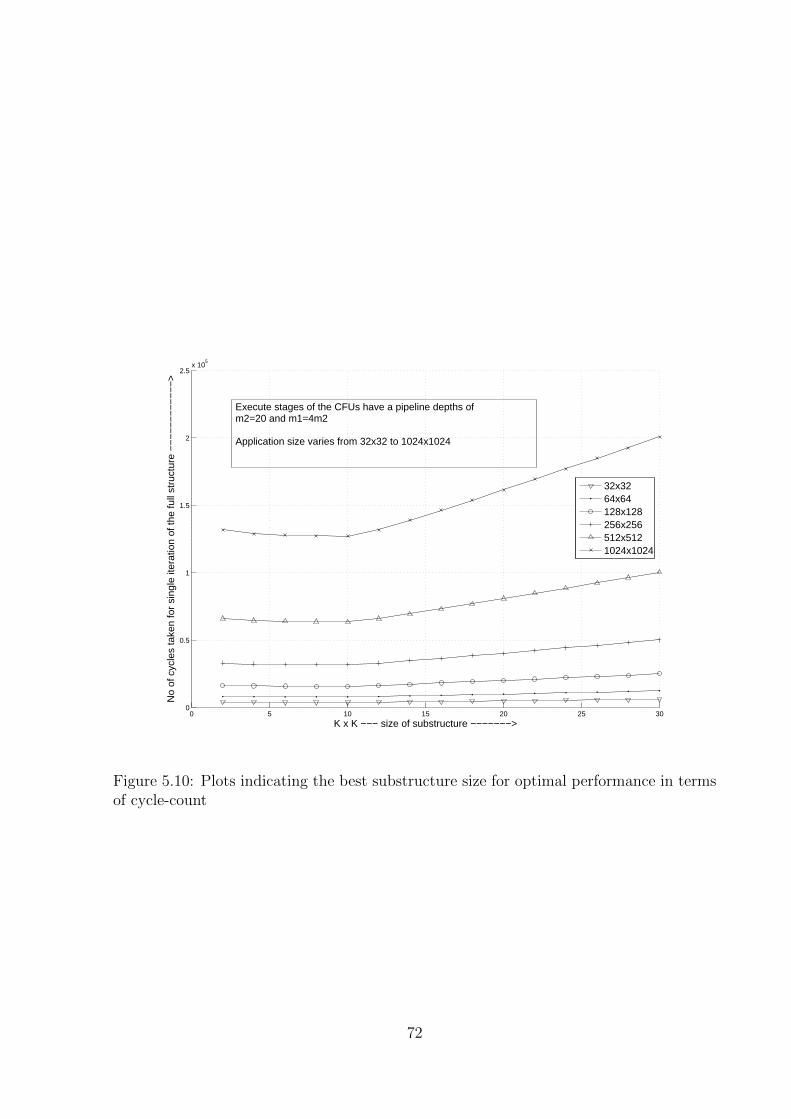
0 5 10 15 20 25 300
0.5
1
1.5
2
2.5x 10
5
K x K −−− size of substructure −−−−−−−>
No
of c
ycle
s ta
ken
for
sing
le it
erat
ion
of th
e fu
ll st
ruct
ure
−−
−−
−−
−−
−−
−−
>
32x3264x64128x128256x256512x5121024x1024
Execute stages of the CFUs have a pipeline depths ofm2=20 and m1=4m2
Application size varies from 32x32 to 1024x1024
Figure 5.10: Plots indicating the best substructure size for optimal performance in termsof cycle-count
72

0 5 10 15 20 25 30 35 40 45 500.2
0.4
0.6
0.8
1
1.2
1.4
1.6
1.8
2
2.2x 10
4
pipeline depth of the execute stage of the CFU −−−−−>
Nor
mal
ized
cyc
le c
ount
for
sing
le it
erat
ion
−−
−−
−−
−>
2x24x46x68x810x1012x1214x1416x1618x1820x20
Application size is 512x512
Substructure size varies from 2x2 to 20x20
Figure 5.11: Plots showing the normalized cycle-counts with the change in pipe-line depthfor different substructure sizes
73
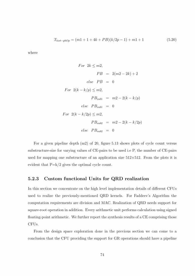
Tlast−phOp = (m1 + 1 + 4k + PB)(k/2p− 1) +m1 + 1 (5.20)
where
For 2k ≤ m2,
PB = 2(m2− 2k) + 2
else PB = 0
For 2(k − k/p) ≤ m2,
PBsub1 = m2− 2(k − k/p)
else PBsub1 = 0
For 2(k − k/2p) ≤ m2,
PBsub2 = m2− 2(k − k/2p)
else PBsub2 = 0
For a given pipeline depth (m2) of 20, figure 5.13 shows plots of cycle count versus
substructure-size for varying values of CE-pairs to be used i.e P, the number of CE-pairs
used for mapping one substructure of an application size 512×512. From the plots it is
evident that P=k/2 gives the optimal cycle count.
5.2.3 Custom functional Units for QRD realization
In this section we concentrate on the high level implementation details of different CFUs
used to realize the previously-mentioned QRD kernels. For Faddeev’s Algorithm the
computation requirements are division and MAC. Realization of QRD needs support for
square-root operation in addition. Every arithmetic unit performs calculation using signed
floating-point arithmetic. We further report the synthesis results of a CE comprising those
CFUs.
From the design space exploration done in the previous section we can come to a
conclusion that the CFU providing the support for GR operations should have a pipeline
74
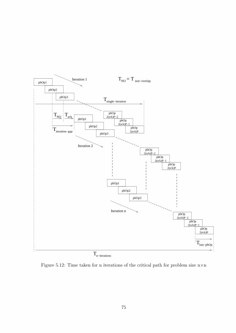
Tlast−phOp
Tn−iterations
Tsingle−iteration
Titeration−gap
TackTNO
T = TNO non−overlap
2(n/k)P−1phOp
2(n/k)PphOp
2(n/k)P−2phOp
2(n/k)P−1phOp
2(n/k)PphOp
2(n/k)P−2phOp
2(n/k)P−1phOp
2(n/k)PphOp
phOp1
phOp1
phOp1
phOp2
phOp3
phOp2
phOp3
phOp2
phOp3
Iteration n
Iteration 1
Iteration 2
phOp2(n/k)P−2
Figure 5.12: Time taken for n iterations of the critical path for problem size n×n
75
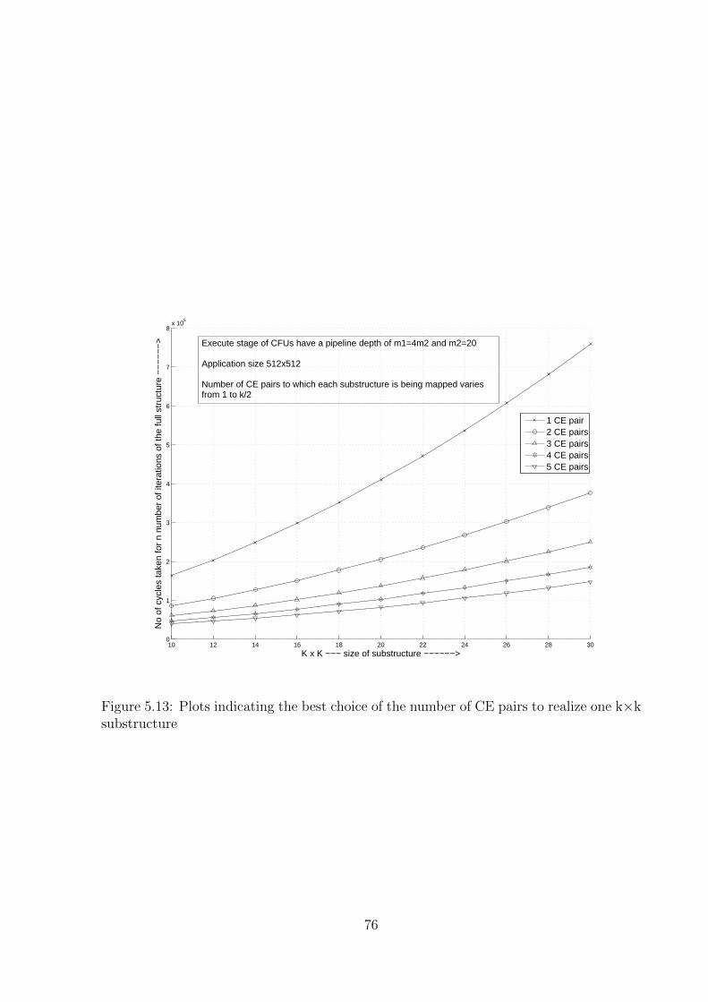
10 12 14 16 18 20 22 24 26 28 300
1
2
3
4
5
6
7
8x 10
5
K x K −−− size of substructure −−−−−−>
No
of c
ycle
s ta
ken
for
n nu
mbe
r of
iter
atio
ns o
f the
full
stru
ctur
e −
−−
−−
−>
1 CE pair2 CE pairs3 CE pairs4 CE pairs5 CE pairs
Execute stage of CFUs have a pipeline depth of m1=4m2 and m2=20
Application size 512x512
Number of CE pairs to which each substructure is being mapped varies from 1 to k/2
Figure 5.13: Plots indicating the best choice of the number of CE pairs to realize one k×ksubstructure
76
depth of 20 for optimal performance. In accordance with that the optimal substructure
size should be 10× 10. Realizing a k× k subarray on k/2 CE pairs results in best perfor-
mance. So we can say that, ultimate performance comes when each 10× 10 substructure
gets mapped on 5 CE-pairs. Hence, each CE would accommodate 10 macro-level instruc-
tions. A 16 slot CE would suffice for this requirement.
GG operation is a combination of square-root and division. CFU1 provides the support
for that. The operand must be in the square root unit input before the calculation process
starts. We used Newtons Iteration Method which is also known as Newton- Raphson
Method to find the root of the input data. CFU1 i.e the amalgamation of Square-root
and division units consumes two sets of data. Xin (refer figure 2.11) comes from the
reservation station (Local Operation Orchestrator(LOpOr)) and R gets retrieved from the
SPM. First multiplication and then division is done one by one and the C and S factors
are generated at consecutive cycles. The division and square root units are pipelined.
Internal register is used to hold the intermediate result generated by the square-root unit.
Once C and S factors are generated GR operations can enter the execution stage.
GR operations are facilitated in CFU2. GR operations are combined MAC operations.
An enhanced MAC unit (shown in figure 5.14) serves the purpose for breaking each com-
plex GR operation into four RISC type MAC instructions and execute them sequentially
in a pipelined manner without avoiding the data-dependency constraint. As mentioned
previously, number of data-independent GR operations at a time is equal to the num-
ber of operations in a row of the substructure. During computation phase the infor-
mation regarding the number of instructions that can be broken into RISC type MAC
operations and launched onto the enhanced MAC unit comes from a register namely
Row Length Register (refer figure 5.14). While loading the configuration data i.e the
meta-data into the CE the substructure size value is also written onto that register. One
controller unit (partially depicted in figure 5.15) generates the necessary control signals
to ensure the correct data movements. Without any alternation in the hardware design
the CE with these set of CFUs can be used to realize the core computations of Faddeev’s
Algorithm mentioned previously.
77
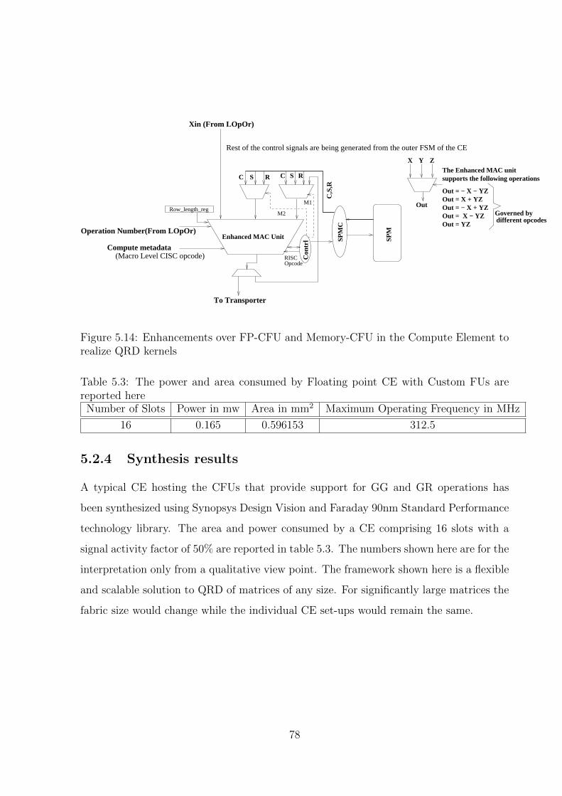
RISCOpcode
Out = − X − YZOut = X + YZOut = − X + YZOut = X − YZOut = YZ
C S R RSC
C,S
,R
SP
MC
SP
M
Con
trl
M1
M2
Enhanced MAC Unit
Row_length_reg
X Y Z
Out
The Enhanced MAC unitsupports the following operations
different opcodesGoverned by
Rest of the control signals are being generated from the outer FSM of the CE
Xin (From LOpOr)
Operation Number(From LOpOr)
Compute metadata(Macro Level CISC opcode)
To Transporter
Figure 5.14: Enhancements over FP-CFU and Memory-CFU in the Compute Element torealize QRD kernels
Table 5.3: The power and area consumed by Floating point CE with Custom FUs arereported hereNumber of Slots Power in mw Area in mm2 Maximum Operating Frequency in MHz
16 0.165 0.596153 312.5
5.2.4 Synthesis results
A typical CE hosting the CFUs that provide support for GG and GR operations has
been synthesized using Synopsys Design Vision and Faraday 90nm Standard Performance
technology library. The area and power consumed by a CE comprising 16 slots with a
signal activity factor of 50% are reported in table 5.3. The numbers shown here are for the
interpretation only from a qualitative view point. The framework shown here is a flexible
and scalable solution to QRD of matrices of any size. For significantly large matrices the
fabric size would change while the individual CE set-ups would remain the same.
78
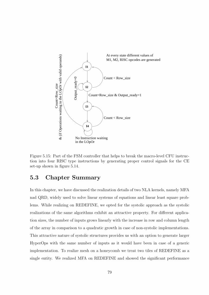
I1
I2
I3
I4
At every state different values ofM1, M2, RISC opcodes are generated
Count < Row_size
Count=Row_size & Output_ready=1
Count < Row_size
No Instruction waitingin the LOpOr
& (
if O
pera
tions
wai
ting
in th
e L
OpO
r w
ith v
alid
ope
rand
s)C
ount
=R
ow_s
ize
Out
put_
read
y=0
Figure 5.15: Part of the FSM controller that helps to break the macro-level CFU instruc-tion into four RISC type instructions by generating proper control signals for the CEset-up shown in figure 5.14.
5.3 Chapter Summary
In this chapter, we have discussed the realization details of two NLA kernels, namely MFA
nad QRD, widely used to solve linear systems of equations and linear least square prob-
lems. While realizing on REDEFINE, we opted for the systolic approach as the systolic
realizations of the same algorithms exhibit an attractive property. For different applica-
tion sizes, the number of inputs grows linearly with the increase in row and column length
of the array in comparison to a quadratic growth in case of non-systolic implementations.
This attractive nature of systolic structures provides us with an option to generate larger
HyperOps with the same number of inputs as it would have been in case of a generic
implementation. To realize mesh on a honeycomb we treat two tiles of REDEFINE as a
single entity. We realized MFA on REDEFINE and showed the significant performance
79

improvement in comparison to GPP. QRD kernel has been used as case study to explore
the design space of the solution. We started with any n × n problem size. From the
mathematical model of the execution latency of the whole application we suggest that
optimal substructure size to be realized on CE pair is 10× 10 or 12× 12. In accordance
to that, to reduce the pipeline bubbles incurred while execution, we came to a design
decision that with a pipeline depth of 20 in the CFU we get optimal cycle count. We
have further investigated that realization of a k×k subarray on k/2 CE pairs comes with
most optimal solution in terms of execution latency. These numbers helps us to predict a
priori the maximum size of an application or the substructure of the application that can
be realized on REDEFINE fabric simultaneously. This maximum size is nothing but the
optimal loop unrolling factor for that application that the compiler will generate before
the code generation phase.
80
Chapter 6
Conclusion and Future work
6.1 Summary
In this thesis, we presented an overview of Systolic array architectures along with the
associated merits and demerits. Structural rigidity inherent to the ASIC realizations of
Systolic Arrays restricts their usage in the embedded domain. GPPs on the other hand
offers better flexibility at the cost of significant performance degradation. Ever growing
complexity of GPPs has led to a shift in focus towards Coarse-Grain Reconfigurable
(CGRA) platforms which usher in the paradigm of simple reconfigurable hardware with
high compute capacity. Here the realization details of Systolic Algorithms on a CGRA
platform, namely REDEFINE has been discussed.
In this thesis our main emphasis was on the realization of Numerical Linear Alge-
bra (NLA) kernels on REDEFINE. Faddeev’s Algorithm and QR Decompositions were
the two NLA kernels of our interest, because of their wide-spread usage in problems like
solving systems of linear equations and linear least square problems. Systolic solutions for
these NLA kernels have been targeted on REDEFINE. To meet the expected performance
various NLA-specific enhancements were proposed. By providing support for persistent
HyperOps, the relaunching overhead of HyperOps which get repeatedly executed, was
avoided. In case of streaming applications like NLA kernels it has shown significant im-
provement in performance. Push model has reduced delay involved in global memory
81
access. Memory subsystems integrated with the Compute Elements (CE) in the form of
SPMs were used to alleviate the effect of lengthy memory transactions on overall per-
formance. Core computations in the NLA kernels were identified for acceleration using
hardware assists. The REDEFINE framework allows application-architecture designers
to fuse multiple basic operations into a coarse grain operation (like MAC, GG and GR
operations here) by extending the instruction set. Such operations can be executed atom-
ically. We designed hardware assist for the above mentioned operation in the form of
a CFU and integrated it with the CEs. Presence of a smart flow-control scheme (by
philosophy analogous to that of wavefront arrays) has ensured consistent data-exchange
between producer and consumer nodes. As mentioned before REDEFINE is a HyperOp
execution engine. Since an arbitrarily large dataflow graph cannot be mapped onto an
execution fabric of finite size, it is imperative to partition the dataflow graph before ex-
ecution. The transfer latency of such a subgraph (i.e. a HyperOp) of the DFG has a
direct impact on the overall execution time. It has been observed that HyperOp launch
latency increases with the HyperOp size at a slower rate when compared to the time
taken for executing the instructions inside the HyperOp. Moreover there is a fixed offset
associated with the HyperOp launch latency. Therefore, for a given DFG (i.e. a fixed
number of instructions) the optimal overall execution time can be achieved by creating
HyperOps of size close to the maximum capacity of the fabric (which in turn dictates the
maximum size of a HyperOp). We have shown that bigger inner-loops in applications
related to matrices (which is translated to bigger sized HyperOps) result in lower execu-
tion latencies. However, limitation on maximum number of inputs does not allow us to
increase the HyperOp size beyond a certain limit. In this context systolic realizations of
the same algorithms exhibit an attractive property. The number of inputs grow linearly
with matrix row-number (and column-number) as opposed to a quadratic growth in case
of a standard non-systolic implementation. This characteristic enables us to create bigger
HyperOps with the same number of inputs. We showed that algorithm-aware compila-
tion techniques ensure creation of such HyperOps of optimal size which leads to improved
performance.
82

A proposition to realize the Systolic Array architecture pertaining to Faddeev’s Algo-
rithm was brought about. It was shown that on an average the performance of REDEFINE
is 29× faster than GPPs while running Faddeev’s Algorithm kernels developed in HLL.
QRD has been used as a case study to explore the design space of the proposed solution on
REDEFINE. We derived the optimal sub-array size, i.e Hyper Op size to be realized per
CE to achieve optimal performance (through a mathematical modeling of the execution
latencies of the solution). In order to further reduce execution latency, we reduced the
number of pipeline bubbles by deriving an optimal pipeline depth of the core execution
units or CFUs. We also evaluated the optimal number of CE-pairs to be used for realizing
a sub-array of a given size.
It is also observed that a hand-crafted CFU capable of executing more coarse grained
compound instructions reduces communication overhead. The framework used to realize
QRD can be generalized for the realization of other decomposition algorithms like LU,
Faddeev’s Algorithm, Gauss-Jordon etc with different CFU definitions.
6.2 Future Work
The importance of the MFA and QRD algorithms discussed in this thesis is unlikely to
fade away in future because of their prominent presence in the domain of NLA. The most
generic solution providers, i.e GPPs are not able to cope up with the need for fast enough
reconfigurable solutions. The reconfigurable computing architectures like REDEFINE (a
CGRA) can be concisely described as Hardware-On-Demand, general purpose custom
hardware, or a hybrid approach between ASIC and GPP. In this thesis a new perspective
to view the systolic realizations of NLA kernels (MFA and QRD) has been presented. It
can be termed as a translation of the only-hardware or hardware-software co-design to
the reconfigurable computing technology. The methodology used to realize MFA, along
with the design decisions derived during QRD case study can be used to realize an entire
Kalman Filter (KF) as two parallel threads of MFA kernels running concurrently. KF
is extensively used in domains like GPS, Attitude and Heading Reference Systems, Dy-
namic positioning, Inertial guidance system, Speech enhancement, Weather forecasting
83
etc. Henceforth, realization of KF can be an instrumental precursor in providing reconfig-
urable solutions in those aforementioned domains. The compilation framework suggested
in the thesis can be easily extended to other algorithms, be it systolic or non-systolic. The
algorithms should be categorized first depending upon their features that are common.
Design space exploration needs to be performed for every set of algorithms in order to
achieve maximal performance gain with minimal hardware complexity. Fast and smart
hardware assists, i.e the domain specific CFUs can play a critical role in the process of
performance enhancement. Realization of algorithm-aware compiler framework, which
is semi-automatic now, would enable us to go for further fine tunings in the optimiza-
tion process. This would improve the performance that can be achieved by the scheme
presented in this thesis.
Reasoning draws a conclusion, but does not make the conclusion certain, unless the
mind discovers it by the path of experience. — Roger Bacon
84
Acronyms
ASIC Application Specific Integrated Circuit
VLSI Very Large Scale Integration
NLA Numerical Linear Algebra
IC Integrated Circuit
NRE Non Recurring Engineering
GPP General Purpose Processor
CGRA Coarse Grained Reconfigurable Architecture
CE Compute Element
NoC Network on Chip
QRD QR Decomposition
DG Dependence Graph
SFG Signal Flow Graph
FA Faddeevs Algorithm
MFA Modified Faddeevs algorithm
GR Givens Rotation
GG Givens Generation
85
PE Processing Element
LUTs Look Up Tables
CLBs Configurable Logic Blocks
FPGA Field Programmable Gate Array
FPOA Field Programmable Object Array
HLL High Level Language
HL HyperOp Launcher
LSU Load Store Unit
IHDF Inter HyperOp Data For-warder
HRM Hardware Resource Manager
CFUs Custom Function Units
RB Resource Binder
DFG Data Flow Graph
HSL HyperOp Selection Logic
GWMU Global Wait-Match Unit
LWMU Local Wait Match Unit
VC Virtual Channel
SPM Scratch-Pad Memory
SPMC Scratch-Pad Memory Controller
DSP Digital Signal Processing
KF Kalman Filter
86
Bibliography
[1] M. A. Bayoumi, P. Rao, and B. Alhalabi, “VLSI parallel architecture for kalman filter: an
algorithm specific approach,” J. VLSI Signal Process. Syst., vol. 4, no. 2-3, pp. 147–163,
1992.
[2] A. Fell, M. Alle, K. Varadarajan, P. Biswas, S. Das, J. Chetia, S. K. Nandy, and R. Narayan,
“Streaming fft on redefine-v2: an application-architecture design space exploration,” in
CASES ’09: Proceedings of the 2009 international conference on Compilers, architecture,
and synthesis for embedded systems. New York, NY, USA: ACM, 2009, pp. 127–136.
[3] H. Kung and C. Leiserson, “Systolic Arrays for VLSI,” in Sparse Matrix Symposium. SIAM,
1978, pp. 256–282.
[4] H. Kung, “Why Systolic Architectures?” in IEEE Computer 15(1), 1982, pp. 256–282.
[5] S. Y. Kung, VLSI array processors. Englewood Cliffs, New Jersy 07632, USA: Prentice
Hall Publishers Inc., 1988.
[6] T. U. Kaiserslautern, “The configware page,” 2007. [Online]. Available:
http://configware.org
[7] ——, “The flowware page,” 2007. [Online]. Available: http://flowware.net
[8] R. Hartenstein, “Why we need reconfigurable computing education,” in Proceedings of the
1st International Workshop on Reconfigurable Computing Education. IEEE Computer
Society, 2006, pp. 1–11.
[9] P. Biswas, P. P. Udupa, R. Mondal, K. Varadarajan, M. Alle, S. Nandy, and R. Narayan,
“Accelerating numerical linear algebra kernels on a scalable run time reconfigurable plat-
form,” in International symposium on VLSI(ISVLSI), Kefalonia, Greece, 2010.
87
[10] P. Biswas, K. Varadarajan, M. Alle, S. Nandy, and R. Narayan, “Design space exploration
of systolic realization of qr factorization on a runtime reconfigurable platform,” in Inter-
national Symposium on Systems, Architectures, Modeling, and Simulation (SAMOS X),
SAMOS, Greece, 2010.
[11] J. G. Nash and S. Hassen, “Modified Faddeev Algorithm for Matrix Manipulation: an
overview,” in SPIE : Real Time Signal Processing IV, 1984, pp. 39–45.
[12] W. M. Gentleman and H. T. Kung, “Matrix triangularization by systolic arrays,” in So-
ciety of Photo-Optical Instrumentation Engineers (SPIE) Conference Series, ser. Society
of Photo-Optical Instrumentation Engineers (SPIE) Conference Series, vol. 298, Jan. 1981,
pp. 19–+.
[13] M. Alle, K. Varadarajan, A. Fell, N. Joseph, C. R. Reddy, S. Das, P. Biswas, J. Chetia, S. K.
Nandy, and R. Narayan, “REDEFINE: Runtime Reconfigurable Polymorphic ASIC,” ACM
Transactions on Embedded Systems, Special Issue on Configuring Algorithms, Processes and
Architecture, 2008.
[14] M. C. Chen, “Space Time Algorithm: Semantics and Methodology,” in PhD Thesis. Com-
puter Science Department, California Institute of Technology, 1983.
[15] D. I. Moldovan, “On the design of Algorithms for VLSI Systolic Arrays,” in Proceedings of
the IEEE, vol. 71, no. 1. IEEE, January 1983.
[16] W. L. Mirankar, “Space-time repreentations of computational structures,” in Computing.
IEEE Computer Society, 1984.
[17] D. K. Faddeev and V. N. Faddeeva, Computational methods of linear algebra. Leningrad:
”Nauka”, Leningrad. Otdel., 1975, vol. 54.
[18] A. Ghosh and P. Paparao, “Performance of modified faddeev algorithm on optical proces-
sors,” Optoelectronics, IEE Proceedings J, vol. 139, no. 5, pp. 325–330, Oct 1992.
[19] M. Zajc, R. Sernec, and J. Tasic, “An efficient linear algebra soc design: implementa-
tion considerations,” in Electrotechnical Conference, 2002. MELECON 2002. 11th Mediter-
ranean, 2002, pp. 322–326.
88
[20] G. Golub and C. V. Loan, Matrix Computations. John Hopkins Press, 1989.
[21] T. K. Moon and W. C. Stirling, Mathematical methods and algorithms for signal processing.
pub-PH:adr: Prentice-Hall, 2000.
[22] J. G. McWhirter, “Recursive least squares minimization using a systolic array,” in REAL
Time signal processing VI, Proc. SPIE, 1983, pp. 105–112.
[23] A. N. Satrawala, K. Varadarajan, M. Alle, S. K. Nandy, and R. Narayan, “REDEFINE:
Architecture of a SOC Fabric for Runtime Composition of Computation Structures,” in
FPL ’07: Proceedings of the International Conference on Field Programmable Logic and
Applications, Aug. 2007.
[24] N. Joseph, C. R. Reddy, K. Varadarajan, M. Alle, A. Fell, S. K. Nandy, and R. Narayan,
“RECONNECT: A NoC for polymorphic ASICs using a Low Overhead Single Cycle
Router,” in ASAP ’08: Proceedings of the 19th IEEE International Conference on Ap-
plication specific Systems, Architectures and Processors, Lueven, Belgium, Jul. 2008.
[25] M. Alle, K. Varadarajan, , A. Fell, S. K. Nandy, and R. Narayan, “Compiling Techniques
for Coarse Grained Runtime Reconfigurable Architectures,” in ARC’09: Proceedings of the
5th IEEE International Workshop on Applied Reconfigurable Computing, jul 2008.
[26] M. Alle, K. Varadarajan, N. Joseph, C. R. Reddy, A. Fell, S. K. Nandy, and R. Narayan,
“Synthesis of Application Accelerators on Runtime Reconfigurable Hardware,” in ASAP
’08: Proceedings of the 19th IEEE International Conference on Application specific Systems,
Architectures and Processors, Lueven, Belgium, Jul. 2008.
[27] K. Vinod, Arvind, and K. Pingali, “A Dataflow Architecure with
tagged Tokens,” Massachusetts Institute of Technology, Laboratory for Com-
puter Science, Tech. Rep. MIT/LCS/TM-174, Sep. 1980. [Online]. Available:
http://www.lcs.mit.edu/publications/specpub.php?id=173
[28] Chris Lattner and Vikram Adve, “LLVM: A Compilation Framework for Lifelong Program
Analysis & Transformation,” in CGO ’04: Proceedings of the international symposium on
Code generation and optimization, Palo Alto, California, 2004.
89
[29] W. J. Dally, “Virtual-Channel Flow Control,” IEEE Transactions on Parallel and Dis-
tributed Systems, vol. 3, no. 2, pp. 194–205, 1992.
90