Hardware and Software Study of Active Noise Cancellation

By

Riggi Aquino

&

Jacob Lincoln

Senior Project

ELECTRICAL ENGINEERING DEPARTMENT

California Polytechnic State University

San Luis Obispo

2012

2

ABSTRACT

Noise cancellation involves removing an unwanted noise while keeping the source sound.

The source sound may consist of speech, music played from a device such as an iPod or a

computer, or no sound at all. The objective of this project is to study the process of noise

cancellation both as hardware and as software. The hardware will consist of building a noise

cancelling circuit that uses headphones as an output, a microphone to pick up the noise to be

cancelled and, if desired, a source sound. The software portion of the experiment will use

MATLAB to simulate the hardware circuit as well as simulate other methods: filtering unwanted

signal, a pi phase shift for inverting the noise signal, the least mean squares algorithm, and the

recursive least squares algorithm. The hardware solution works well with periodic noise but has

difficulty removing noise from non-periodic noise. The software solution using adaptive filtering

works better than the hardware solution but only with periodic noise. Difficulties encountered

include the kinds of noise that can be canceled and the time delay internal to the circuit.

3

TABLE OF CONTENTS

List of Tables..................………………………………………………......................... page 4

List of Figures.................................................................................................................. page 5

1. Introduction………………………………………………………............................. page 6

2. Hardware Approach………………………………………...………….…………… page 7

2.1. Components................................................................................................. page 8

2.2. Idea behind the Circuit…………………………………………..………... page 8

2.3. Testing and Results……………………………………………….............. page 10

2.4. Troubleshooting…………………………………………………............... page 14

2.5. Future Work……………………………………………………................. page 15

3. Software Approach………………………………………………………..................page 16

3.1. Test #1: Simulating the Hardware Circuit………………….…..………… page 20

3.2. Test #2: Designing a Low-Pass……….……………...................................page 23

3.3. Test #3: Frequency Domain Phase Shift………………………..………… page 25

3.4. Test #4: Least Mean Squares……………………………………………... page 30

3.5. Test #5: Recursive Least Squares…………………….…………………... page 34

3.6. Future Work……………………………………………………................. page 37

4. Conclusion…………………………………………….……………………………. page 38

5. References………………………………………….……………………………….. page 39

Appendices

Appendix A: MATLAB Code……………………………………..................... page 40

Appendix B: Component Specifications………………………………………. page 46

Appendix C: Component Costs……...............................................…………... page 48

Appendix D: Analysis of Senior Project Design Form………………………… page 49

4

LIST OF TABLES

Table I: Selected Components Used for Noise Cancelling Hardware (Figure 1)…...… page 7

LIST OF FIGURES

Figure 1: Circuit Diagram of Noise Cancelling Hardware…………………….……… page 7

Figure 2: Block Diagram of Noise Cancelling Circuit………………………………… page 9

Figure 3: Completed Construction of Noise Cancelling Circuit ……………………… page 9

Figure 4: Left-Side Output Stage 1 (channel 1: output after amplification; channel 2: input

signal)…....…....................................................................................................... page 10

Figure 5: Right-Side Output Stage 1 (channel 1: output after amplification; channel 2: input

signal).................................................................................................................. page 11

Figure 6: Left-Side Output Stage 2 (channel 1: output after inversion; channel 2: input

signal).................................................................................................................. page 11

Figure 7: Right-Side Output Stage 2 (channel 1: output after inversion; channel 2: input

signal)................................................................................................................... page 12

Figure 8: Left-side Output Stage 3 (channel 1: output after noise signal (white noise) summed

with source signal (sine wave); channel 2: input source signal (sine wave))...... page 13

Figure 9: Right-Side Output Stage 3 (channel 1: output after noise signal (white noise) summed

with source signal (sine wave); channel 2: input source signal (sine wave))...... page 13

Figure 10: Magnitude Frequency Response of 1 kHz Sinusoid……….......................... page16

Figure 11: Magnitude Frequency Response of 440 Hz Sinusoid……………................ page 17

Figure 12: Magnitude Frequency Response of Heat Gun …………………….……….. page17

Figure 13: Magnitude Frequency Response of Jingling Keys………..………………... page 18

Figure 14: Magnitude Frequency Response of an Electric Fan ……………..………… page 18

Figure 15: Magnitude Frequency Response of a Quiet Room …………….………….. page 19

Figure 16: Magnitude Frequency Response of a Speech .wav File………….………… page 19

Figure 17: Speech Waveform …………………………………………...…………….. page 21

Figure 18: Heat Gun Waveform ……………………………………….……………… page 21

5

Figure 19: Inverted Heat Gun Waveform …………………………………….………….. page 22

Figure 20: Combined Heat Gun and Speech Waveform …………………..….…………. page 22

Figure 21: Summation of Heat Gun, Inverted Heat Gun, and Speech Output Waveform... page 23

Figure 22: Magnitude Frequency Response of Low-pass Filter Output …….…………… page 24

Figure 23: 1 kHz Sinusoid and its Inverse ..............................................………………… page 26

Figure 24: Summation of Non-Inverted and Inverted Sinusoid ………............…………. page 26

Figure 25: 1 kHz Sinusoid and a Delayed, Inverted Sinusoid …………………..……….. page 27

Figure 26: Summation of 1 kHz Sinusoid and a Delayed, Inverted Sinusoid …………… page 27

Figure 27: Heat Gun and its Inverse ………….........................................……………….. page 28

Figure 28: Summation of Heat Gun and its Inverse ………………….………………….. page 28

Figure 29: Heat Gun Signal and a Delayed, Inverted Heat Gun Signal……….…………. page 29

Figure 30: Summation of Heat Gun Signal and a Delayed, Inverted Heat Gun Signal ..... page 29

Figure 31: General Adaptive Filter Block Diagram ……………...................................... page 30

Figure 32: LMS Mean Square Error for 1 kHz Sinusoid (No Delay) …….……………… page 32

Figure 33: LMS Mean Square Error for 1 kHz Sinusoid d)……………....………………. page 32

Figure 34: LMS Mean Square Error for Heat Gun Signal (No Delay)………....………… page 33

Figure 35: LMS Mean Square Error for Heat Gun Signal (1 second Delay) ...................... page 33

Figure 36: RLS Mean Square Error for 1 kHz Sinusoid (No Delay) .................................. page 35

Figure 37: RLS Mean Square Error for 1 kHz Sinusoid (1 second Delay).......................... page 36

Figure 38: RLS Mean Square Error for Heat Gun Signal (No Delay) ……………...……. page 36

Figure 39: RLS Mean Square Error for Heat Gun Signal (1 second Delay).……………... page 37

6

1. INTRODUCTION

Noise is any unwanted disturbance present in a signal. Noise cancellation can be used in

areas where noise can be harmful to ones hearing, such as: engine rooms or aircraft runways. In

signal processing, noise is data within the wanted signal that carries no real value. Typically,

signals are stronger without noise which gives a better signal to noise ratio The study of

cancelling noise from a wanted signal arises from need to achieve stronger signal to noise ratios.

There are two techniques for cancelling noise: passive noise reduction and active noise

cancellation. [7]

Headphones that utilize passive noise reduction often use material that blocks some

sound waves from entering the user’s ears. The best headphones for passive noise reduction are

circum-aural (i.e. covering ears completely). Circum-aural headphones block more incoming

sound waves due to more layers of high density foam. [7] The disadvantage of passive noise

reduction is not all of the ambient noise will be cancelled. Some of the noise, no matter the

method for passive noise cancellation, will make it to the user’s ear. In contrast, active noise

cancellation employs a different approach to noise reduction.

Headphones that utilize active noise cancellation apply different techniques. Active noise

cancellation involves creating a supplementary signal that deconstructively interferes with the

outside, ambient noise. [7] The disadvantage of active noise cancellation is the compromise

made in audio quality as well as the price. Whether the process is done hardware or software

with a DSP chip, the unwanted signal and source signal will share the same frequency content,

leading to cancellation of both.

In theory, the best approach to cancelling noise would be to take the noise signal, invert

it, and add the input and inverted signals such that they add deconstructively. This is the basic

approach used for noise cancelling headphones. This project explores this basic idea of noise

cancellation from a hardware and software approach.

7

2. HARDWARE APPROACH

Figure 1: Circuit Diagram of Noise Cancelling Hardware

Table I: Selected Components Used for Noise Cancelling Hardware (Figure 1)

Label Component Value

R1 Resistor 4.7kΩ

R2-3 Resistor 2.2kΩ

R4-5 Resistor 1MΩ

R6-7 Resistor 1kΩ

R8-9 Resistor 33kΩ

R10-13, R15-18 Resistor 10kΩ

R14, R23 Dual-Gang Potentiometer 100kΩ

R19-20 Resistor 100kΩ

R21-22 Resistor 47Ω

IC1-3 Integrated Circuit NE5532

C1 Electrolytic Capacitor 33µF

C2-3 Mylar Capacitor 0.01µF

C4-5 Electrolytic Capacitor 10µF

S1 DPDT Switch

J1-3 1/8 Inch Audio Jack

8

2.1. Components:

R1 and C1 decouple the bias voltage from the power supply by being placed in a voltage

dividing network. R8 and R6 were chosen to be 33kΩ and 1kΩ for a gain of 31dB for the

amplifying stage. A large value for R4 was chosen (1MΩ) to give a good ground reference for

the amplifying stage. C2/R4 and C4/R6 are high-pass filters blocking any DC before the

amplifier. Lower capacitor values are chosen for these, 0.01µF. The next stage is the unity gain

inverting amplifiers. So 10kΩ resistors were chosen for R10 and R12 to keep unity gain. The

gain of the last stage (summing stage) is set by R19 and R15, which were chosen to be 100kΩ and

10kΩ. R17 is added to create a summing amplifier, chosen to be 10kΩ to interact with the 100kΩ

potentiometer logarithmically. Since this is stereo there is a right and left, so configuration and

set up is mirrored for the opposite side. [10]

2.2. Idea behind the Circuit:

The noise cancelling circuit is composed of three separate stages. The first stage (IC1a-b)

is a non-inverting amplifier stage. This stage simply takes the input from the audio jack (J1) and

amplifies the signal. Amplifying this signal is crucial since the microphone produces a smaller

signal that is difficult to work with. The gain of this stage is set by one plus R8 and R6 (33kΩ and

1kΩ for a gain of approximately 31dB).

The second stage of the circuit (IC2a-b) is a phase inverting configuration that inverts the

amplified signal from the first stage. This stage is supposed to invert the phase so that the output

added with the ambient sound from outside the headphones deconstructively interferes.

The DPDT switch (S1) was added to help with the timing delay issues the circuit has.

That is the time at which the user hears the noise from outside the headphones must match the

time at which the circuit is producing the inverting noise. The switch is to help with this timing

issue. Switching the switch to non-inverting or inverting can help with the timing of the ambient

noise the user hears. This is determined by the user, if the noise is quieter in the non-inverting

position then the delay was significant enough to cause it to be out of phase with the ambient

noise. The distance the microphone is from the user’s ear also helps with the timing delays.

These delays are produced from the signal traveling through the circuit and back to the user’s

ears.

The potentiometer (R14) is used to attenuate the signal from the second stage

(microphone). Noise heard by the user will most likely be muffled due to the headphones

covering a portion of the ear. Attenuating the signal produced by the microphone will help

match the amplitudes of the ambient noise and the output of the circuit.

Last stage of the noise cancelling circuit is a summing, non-inverting, amplifying stage.

The gain of this circuit is set by R19 and R15, and R17 is essential to making this stage a

summing op-amp. Summing is only used when the user is also listening to music (plugged into

9

audio jack, J2). Modified noise from the second stage and the music from J2 will be added

together and sent to the output at J3. This allows the user to hear their music while the ambient

noise is still being cancelled by deconstructive interference.

In summary, the noise signal is amplified and then inverted. This noise is produced by a

microphone connected to audio jack, J1. Amplified and inverted noise is produced at the output

of the circuit, thus, deconstructively interfering with the ambient noise.

Figure 2: Block Diagram of Noise Cancelling Circuit

Figure 3: Completed Construction of Noise Cancelling Circuit

Amplifying

Stage

Inverting

Stage Summing

Stage

Noise Input

Source Signal

Output

10

2.3. Testing and Results

The circuit is essentially a mirror image of itself. Due to being stereo noise, the circuit

has a left and right side, contributing to the left and right outputs of headphones. This allows

testing to be conducted on a single side.

First tested the left-side of the circuit amplifier stage with a 100 mVpp 1 kHz sine wave

inputted on J1. This value had to be small (100mVpp) due to clipping. Clipping occurred at an

input of roughly 140mVpp. The wave got amplified to a 6.75Vpp 1 kHz sine wave.

Figure 4: Left-Side Output Stage 1 (channel 1: output after amplification; channel 2: input signal)

11

Then the right-side amplifier stage was tested using the same input, 100 mVpp 1 kHz sine

wave. The signal was amplified to 6.85 Vpp 1 kHz sine wave. Clipping occurred at an input of

140 mVpp.

Figure 5: Right-Side Output Stage 1 (channel 1: output after amplification; channel 2: input signal)

Second stage inversion was then tested using the same signal, 100 mVpp1 kHz sine wave.

Left-side was first tested for inversion. Clipping occurred at 140 mVpp.

Figure 6: Left-Side Output Stage 2 (channel 1: output after inversion; channel 2: input signal)

12

Right-side, second stage inversion texted with the same input, 100mV 1 kHz sine wave.

Clipping occurred at 140 mVpp.

Figure 7: Right-Side Output Stage 2 (channel 1: output after inversion; channel 2: input signal)

With the input only on left-side and another source connected (J2), this is done to show

that the summing stage of the hardware functions properly. We see an inverted signal amplified

according to the attenuation of the potentiometer (R14) with the signal from J2 added to the input

signal from J1. The sine wave appears noisy due to the input signal of white noise from J1 being

added to a sine wave from J2.

13

Figure 8: Left-side Output Stage 3 (channel 1: output after noise signal (white noise) summed with source signal (sine

wave); channel 2: input source signal (sine wave))

With the input only on right-side and another source connected (J2). We see an inverted

signal amplified according to the attenuation of the potentiometer (R14) with the signal from J2

added to the input signal from J1. Noisy sine wave is seen on output for the same reason it is

seen on the left side output (figure 8).

Figure 9: Right-Side Output Stage 3 (channel 1: output after noise signal (white noise) summed with source signal (sine

wave); channel 2: input source signal (sine wave))

14

For field testing a sine wave, treated as noise, was played through PC speakers, a

microphone placed near the user’s ear was plugged into J1. Turtle Beach X12 Earforce

headphones were used, these were plugged into J3 (output audio jack). The sine wave (noise)

from the headphones is loud, louder than the outside sine wave. This is due to the attenuation of

the input signal from the microphone. For configuring, start with the circuit in the non-inverted

position, that is the switch (S1) must be switched to allow the first stage to enter the

potentiometer (R14). Attenuate the microphone input using the potentiometer until the least

amount of noise is heard from the headphones (typically as low as possible without completely

shutting off channel). At this point switch to the inverting stage. This process is subjective to

the user and may vary for different individuals.

This method was done several times using different sine waves and different

configurations for the microphone. With the microphone placed as close to the PC speakers as

possible, better results were achieved. The inverting stage (stage 2) produced a much quieter

output than the non-inverting stage (stage 1) just as it had previously done for the microphone

being closer to the user’s ear.

2.4. Troubleshooting

There were many difficulties with this noise cancelling circuit design. The design itself

is intuitive and straight forward. One of the biggest obstacles with this design is understanding

that it does not perfectly cancel ambient noise. This cannot be achieved with the full range of

frequencies heard (20-20 kHz). Market bought noise cancelling headphones typically work well

for certain environments, working well where there are high or low frequencies. For example a

pair of Bose Quiet Comfort 15, work well for frequencies up to 1 kHz, at which point their

ability to cancel noise fails. [3]

Another trouble encountered was the DPDT switch. Several switches were burned out

and lead to incorrect results. This was caused by overheating the switches while soldering the

wires on the leads for connection to the breadboard. When switching to inverting stage (stage 2)

the switch wasn't making correct contact leading to no noise cancellation and wasted time. With

a more rigid DPDT switch this problem was quickly alleviated.

An additional hardware problem was finding microphones that were able to pick up the

signal. Condenser microphones were used; these microphones were mounted to the headphones

with each microphone on either side of the headphones. The thought behind this is that the

microphones mounted directly to the headphones would help with the timing delays involved in

the circuit. After testing, concluded that the condenser microphones were not picking up enough

of the signal to allow the circuit to cancel. For the remainder of the experiment and testing two

microphones were used. One microphone was an amplified microphone attached to the Turtle

Beach X12 Earforce headphones. This microphone worked well for testing with a microphone

15

that is place near the user’s ear. The other microphone used was a Logitech microphone; this

microphone can be place in many different places.

Timing delays were the biggest problem with this noise cancelling circuit. The timing

delay is associated with the time the signal takes to travel through the circuit and back to the

user’s ear. Ambient noise outside the headphones is going to reach the user sooner than the

signal traveling through the circuit. To offset this delay the DPDT switch was added to the

circuit. The idea behind this switch is to switch which stage is going to be passed through the

circuit, which is the amplifying stage or the inverting stage. Timing delay might be large enough

to where the non-inverting signal is already out of phase with the ambient sound heard by the

user. This scenario doesn't occur often; typically the inverting stage is best. The timing delay

through the circuit is not significant enough to cause the non-inverting signal to be out of phase

with the ambient noise heard by the user.

To alleviate the strain on the delay times, different microphone configurations were used.

The first configuration was with the microphone placed near the user's ear; the second

configuration was with the microphone placed near the noise source. With the microphone close

to the user's ear, this would cause the time delay between the user hearing the signal and

microphone detecting the signal to have the least amount of delay. This configuration worked

well using the cancelling approach described above. A separate Logitech microphone was used

and place close to the signal source (PC speakers). This configuration also worked well. The

difference between these two configurations is the adjustment that will need to be done. The

attenuation done by the potentiometer needs to be calibrated according to the position of the

microphone.

2.5. Future Work

The first improvement to the circuit would be designing a printed circuit board (PCB). A

PCB would help alleviate the circuit noise. The circuit noise being the open components on the

breadboard (see Figure 2 above) touching or moving causing noise on the output that is clearly

heard on the headphones. Using a surface mount PCB would miniaturize this circuit making it

easy to add to the headphones.

Using higher quality audio op-amps would be a huge improvement to the circuit.

NE5532 were used for this circuit because of the lower voltage that the IC needs to operate.

Higher quality audio op-amps require higher voltages to turn on. This higher voltage would help

the sound quality of the circuit; the higher voltage would eliminate low voltage clipping (see

testing and results section for clipping present).

16

3. SOFTWARE APPROACH

MATLAB was used to simulate the hardware portion of the study. In order to simulate

properly, the same microphone used in hardware must be used to record various noises. Five

different types of tests were conducted. The first consisted of simulating the inversion of noise

and adding two signals deconstructively. The second test consisted of creating filters so retain or

remove specific frequencies. Test #3 involved using the fast Fourier transform to do a phase shift

which will invert a signal similar to the method of test #1. For test #4 and test #5, adaptive filters

were used; they consist of using the least mean squares and recursive least squares methods. The

types of noise studied include: 100 Hz, 250 Hz, 440 Hz, 1 kHz, 10 kHz sinusoids, a quiet room, a

room with talking students, hum from a computer, an electric fan, a fume extractor, a heat gun,

typing on a keyboard, and jingling keys. The input/source signals consisted of six different

speech .wav files that were recordings of different voices. For this report, only the tests involving

a non-periodic heat gun noise and a periodic 1 kHz sinusoid will be shown to avoid redundancy.

The desired/source signal used for this study will be one speech signal that consists of a male

voice saying, “In a world we must defend.” However, the following section will contain samples

of other noise sources to give an idea of the frequency spectrum for different signals.

Noise Samples

Figure 10: Magnitude Frequency Response of 1 kHz Sinusoid

0 0.5 1 1.5 2 2.5

x 104

0

0.1

0.2

0.3

0.4

0.5

0.6

0.7

Frequency (Hz)

Am

plit

ude

1 kHz Sinusoid Magnitude

17

Figure 11: Magnitude Frequency Response of 440 Hz Sinusoid

Figure 12: Magnitude Frequency Response of Heat Gun

0 0.5 1 1.5 2 2.5

x 104

0

0.1

0.2

0.3

0.4

0.5

0.6

0.7

Frequency (Hz)

Am

plit

ude

440 Hz Sinusoid Magnitude

0 0.5 1 1.5 2 2.5

x 104

0

0.002

0.004

0.006

0.008

0.01

0.012

0.014

Frequency (Hz)

Am

plit

ude

Heatgun Magnitude

18

Figure 13: Magnitude Frequency Response of Jingling Keys

Figure 14: Magnitude Frequency Response of an Electric Fan

0 0.5 1 1.5 2 2.5

x 104

0

1

2

3

4

5

6

7

8x 10

-3

Frequency (Hz)

Am

plit

ude

Jingling Keys Magnitude

0 0.5 1 1.5 2 2.5

x 104

0

0.01

0.02

0.03

0.04

0.05

0.06

0.07

Frequency (Hz)

Am

plit

ude

Fan Magnitude

19

Figure 15: Magnitude Frequency Response of a Quiet Room

Speech Sample

Figure 16: Magnitude Frequency Response of a Speech .wav File

0 0.5 1 1.5 2 2.5

x 104

0

0.5

1

1.5

2

2.5

3

3.5

4

4.5x 10

-3

Frequency (Hz)

Am

plit

ude

Quiet Room Magnitude

0 0.5 1 1.5 2 2.5

x 104

0

0.005

0.01

0.015

Frequency (Hz)

Am

plit

ude

Speech Magnitude

20

From figures 10 and 11, it can be seen that the magnitude response of a sinusoid lies on

its current frequency. To cancel the noise from a sine wave, a filter could be implemented at

specific frequencies to cancel out (notch filter) or avoid (low-pass, high-pass) the noise of a sine

wave. For magnitude responses like in figure 12 (heat gun) and 14 (fan), most of their signal lies

in the lower frequencies. A high-pass filter with a cutoff frequency above 2 kHz could

theoretically cancel most of the noise if the source signal would not be affected. However, from

figure 15, the majority of the desired speech signal lies at lower frequencies. For noise like

jingling keys from figure 13, a simple filter would not work well due to overlap with the

frequency spectrum of the speech signal.

3.1. Test #1: Simulating the Hardware Circuit

The first test involved importing a noise .wav file and a speech .wav file. Since both

sources were separated into two channels, MATLAB was used to add them together. Recalling

the hardware portion, the first stage was used to amplify the noise, the second stage was used to

invert the noise, and the third stage added the noise with its inverted signal.

Since this was a simulation, the first stage was neglected due to amplification not being

required within the software method. The second stage was simulated by multiplying the noise

signal by -1. Finally, the third stage added the inverted noise signal to the original signal which

contained the speech and noise.

The desired speech signal was recorded using the hardware microphone in a quiet room.

The duration of the signal is approximately 4.5 seconds with the actual speech starting at 1.25

seconds and ending at 3 seconds.

21

Figure 17: Speech Waveform

Figure 18: Heat Gun Waveform

0 0.5 1 1.5 2 2.5 3 3.5 4 4.5-1

-0.8

-0.6

-0.4

-0.2

0

0.2

0.4

0.6

0.8

1

Time (seconds)

Am

plit

ude

Speech Signal in Time Domain

0 0.5 1 1.5 2 2.5 3 3.5 4 4.5-0.25

-0.2

-0.15

-0.1

-0.05

0

0.05

0.1

0.15

0.2

0.25

Time (seconds)

Am

plit

ude

Heatgun Signal in Time Domain

22

Figure 19: Inverted Heat Gun Waveform

Figure 20: Combined Heat Gun and Speech Waveform

0 0.5 1 1.5 2 2.5 3 3.5 4 4.5-0.25

-0.2

-0.15

-0.1

-0.05

0

0.05

0.1

0.15

0.2

0.25

Time (seconds)

Am

plit

ude

Inverted Heatgun Signal in Time Domain

0 0.5 1 1.5 2 2.5 3 3.5 4 4.5-1

-0.5

0

0.5

1

1.5

Time (seconds)

Am

plit

ude

Heatgun + Speech Signal in Time Domain

23

Figure 21: Summation of Heat Gun, Inverted Heat Gun, and Speech Output Waveform

As can be seen from the plots above, the noise was not only reduced but was perfectly

cancelled. This was verified with the output .wav file generated by MATLAB. However, in the

real world, one cannot simply multiply -1 to a signal. This problem was addressed during the

next set of tests.

3.2. Test #2: Designing a Low-Pass

By using the fast Fourier transform (FFT) one can see where the frequencies of various

signals lie. With this information, a filter can be built to remove or retain a specific range of

frequencies. Fortunately, MATLAB contains both an FFT and an iFFT function (inverse fast

Fourier transform) [6]. From the FFT plot of the speech sample in figure 16, one can determine

that most of the signal is contained at frequencies lower than 2 kHz.

With this information, a low-pass filter (Butterworth) with cutoff frequency of 2 kHz was

designed. The butter function of MATLAB generates the filter coefficients given the order of the

filter and the cutoff frequency. A filter order of two was used to reduce computation time. When

filtering the speech with heat gun noise, the filter failed to remove the noise due to the heat gun’s

signal being present at low frequencies. When the output signal was played in MATLAB, both

0 0.5 1 1.5 2 2.5 3 3.5 4 4.5-1

-0.8

-0.6

-0.4

-0.2

0

0.2

0.4

0.6

0.8

1

Time (seconds)

Am

plit

ude

Heatgun + Inverted Heatgun + Speech Signal in Time Domain

24

the speech and the heat gun were clearly heard with a noticeable decrease in volume. The

decrease in volume is due to the higher frequencies being filtered out. This same problem also

occurred with the 1 kHz sinusoid noise since the cutoff frequency was 2 kHz.

Transfer Function for Low-Pass Filter:

0.0167 0.0335 0.0167

1 1.602 0.669

Figure 22: Magnitude Frequency Response of Low-pass Filter Output

When using sinusoids of various frequencies as the noise source, the low-pass filter

successfully eliminated any noise above 2 kHz. However, in the real world, a low-pass filter

would not be acceptable to cancel out noise. Using this method for noise cancellation would be

very situational and designed for a specific purpose.

0 0.5 1 1.5 2 2.5

x 104

0

0.002

0.004

0.006

0.008

0.01

0.012

0.014

0.016Low Pass Filter Output of Signal+Heat Gun in Frequency Domain

Frequency (Hz)

Am

plit

ude

25

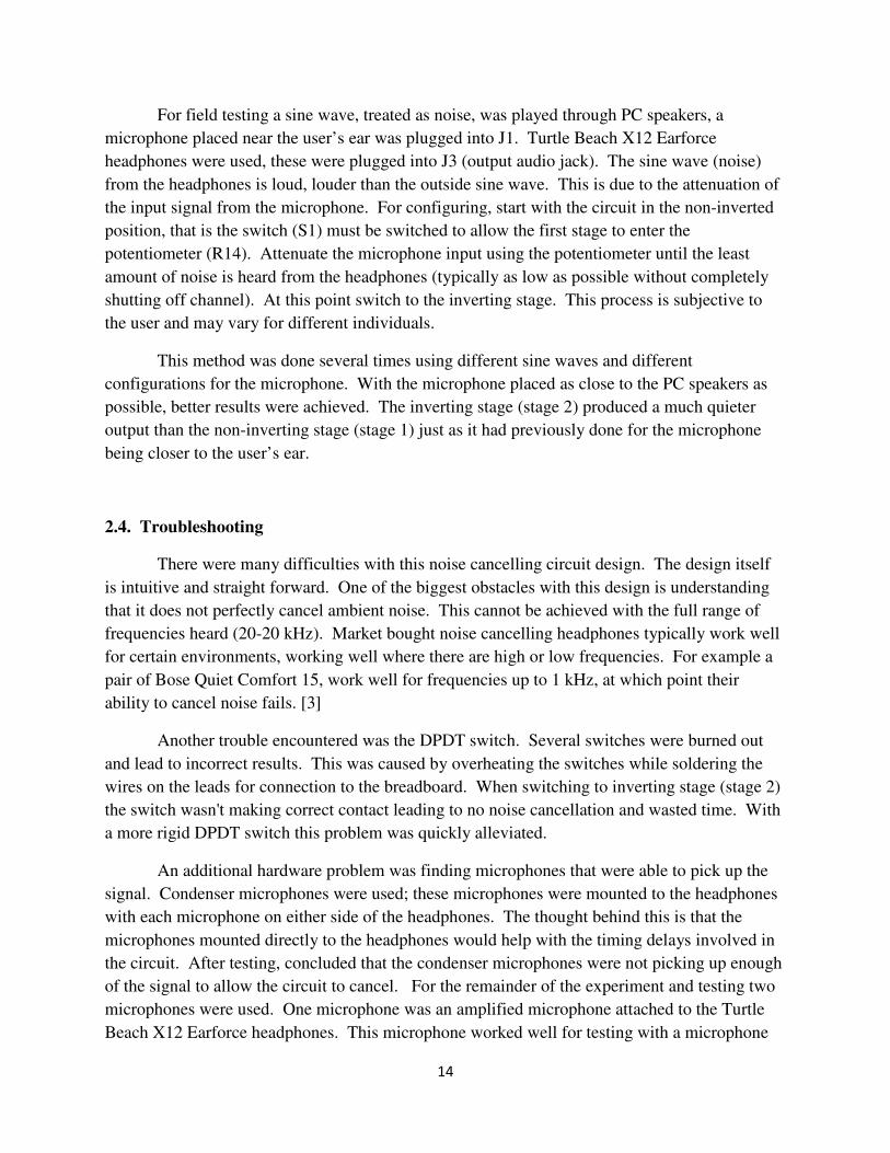
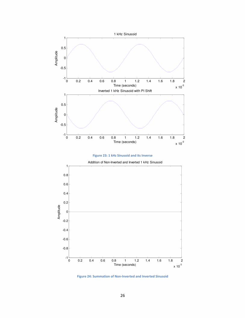
3.3. Test #3: Frequency Domain Phase Shift

The problem encountered during the first simulation test was how to invert a signal using

a method that could be applied to the real world. The solution is to add a π phase shift. When

working in the frequency domain, a π phase shift is similar to inverting a signal. These functions

were used to convert the time domain signals to the frequency domain where the π phase shift

could be done.

!"#$ $ ! 0

%& '

( )*+ )+ · -.

/)*+/ |)+| 1)*+ 1)+ 2

%& '

! 0

26

Figure 23: 1 kHz Sinusoid and its Inverse

Figure 24: Summation of Non-Inverted and Inverted Sinusoid

0 0.2 0.4 0.6 0.8 1 1.2 1.4 1.6 1.8 2

x 10-3

-1

-0.5

0

0.5

1

Time (seconds)

Am

plit

ude

1 kHz Sinusoid

0 0.2 0.4 0.6 0.8 1 1.2 1.4 1.6 1.8 2

x 10-3

-1

-0.5

0

0.5

1

Time (seconds)

Am

plit

ude

Inverted 1 kHz Sinusoid with PI Shift

0 0.2 0.4 0.6 0.8 1 1.2 1.4 1.6 1.8 2

x 10-3

-1

-0.8

-0.6

-0.4

-0.2

0

0.2

0.4

0.6

0.8

1

Time (seconds)

Am

plit

ude

Addition of Non-Inverted and Inverted 1 kHz Sinusoid

27

Figure 25: 1 kHz Sinusoid and a Delayed (1 second), Inverted Sinusoid

Figure 26: Summation of 1 kHz Sinusoid and a Delayed (1 second), Inverted Sinusoid

0 0.2 0.4 0.6 0.8 1 1.2 1.4 1.6 1.8 2

x 10-3

-1

-0.5

0

0.5

1

Time (seconds)

Am

plit

ude

1 kHz Sinusoid

0 0.2 0.4 0.6 0.8 1 1.2 1.4 1.6 1.8 2

x 10-3

-1

-0.5

0

0.5

1

Time (seconds)

Am

plit

ude

Delayed and Inverted 1 kHz Sinusoid with PI Shift

0 0.2 0.4 0.6 0.8 1 1.2 1.4 1.6 1.8 2

x 10-3

-1

-0.8

-0.6

-0.4

-0.2

0

0.2

0.4

0.6

0.8

1Addition of Non-Inverted and Inverted 1 kHz Sinusoid

Time (seconds)

Am

plit

ude

28

Figure 27: Heat Gun and its Inverse

Figure 28: Summation of Heat Gun and its Inverse

0 0.2 0.4 0.6 0.8 1 1.2 1.4 1.6 1.8 2

x 10-3

-0.1

-0.05

0

0.05

0.1

Time (seconds)

Am

plit

ude

Heat Gun Signal

0 0.2 0.4 0.6 0.8 1 1.2 1.4 1.6 1.8 2

x 10-3

-0.1

-0.05

0

0.05

0.1

Time (seconds)

Am

plit

ude

Inverted Heat Gun Signal with PI Shift

0 0.2 0.4 0.6 0.8 1 1.2 1.4 1.6 1.8 2

x 10-3

-1

-0.8

-0.6

-0.4

-0.2

0

0.2

0.4

0.6

0.8

1

Time (seconds)

Am

plit

ude

Addition of Non-Inverted and Inverted Heat Gun Signals

29

Figure 29: Heat Gun Signal and a Delayed (1 second), Inverted Heat Gun Signal

Figure 30: Summation of Heat Gun Signal and a Delayed (1 second), Inverted Heat Gun Signal

0 0.2 0.4 0.6 0.8 1 1.2 1.4 1.6 1.8 2

x 10-3

-0.1

-0.05

0

0.05

0.1

Time (seconds)

Am

plit

ude

Heat Gun Signal

0 0.2 0.4 0.6 0.8 1 1.2 1.4 1.6 1.8 2

x 10-3

-0.1

-0.05

0

0.05

0.1

Time (seconds)

Am

plit

ude

Delayed and Inverted Heat Gun Signal with PI Shift

0 0.2 0.4 0.6 0.8 1 1.2 1.4 1.6 1.8 2

x 10-3

-0.15

-0.1

-0.05

0

0.05

0.1

Time (seconds)

Am

plit

ude

Addition of Non-Inverted and Inverted Heat Gun Signals

30

As can be seen from the plots above, adding an input signal with the same signal but π

shifted in the frequency domain will output no signal. This method will work for both periodic

(sinusoid) and non-periodic (heat gun) signals. However, figures 23 and 27 do not take into

account the time delay that would be encountered in a physical circuit when using a microphone.

Delay is not an issue for software, but in order to simulate actual hardware, delay should be

considered. When adding an input signal with a time delayed version of the same signal, a π shift

in the frequency domain will no longer zero the output signal as seen in figures 26 and 30. This

method also implies that one will have the source signal and noise signal in separate channels

otherwise both the source and noise will be cancelled. If there were a way to estimate the time

delay, this method could work, but the estimated time delay would have to be perfect.

3.4. Test #4: Least Mean Squares

This section discusses the use of adaptive filters. If there were no time delay to take into

account, the methods applied in the previous tests would be all that is needed. However, in the

real world, one will not likely have the a priori information required to cancel out the noise that

will be heard (i.e. one won’t know the type of noise that will be heard).

Adaptive filters update their filter coefficients iteratively using algorithms like least mean

squares or recursive least squares [1]. For noise cancellation in this project, an adaptive filter will

take two inputs. The first input is the desired signal and it consists of the signal s(n) and noise

X(n); the second input is a reference noise x(n) that relates in some way to the noise heard in the

desired signal. The reference noise in this case will be the delayed version of the noise heard

with the desired signal. The output e(n) is the error signal which consists of the desired signal

with cancelled noise.

Figure 31: General Adaptive Filter Block Diagram

Desired signal: d(n) = s(n) + X(n)

Reference noise: x(n)

Filter coefficients

w(n)

Error signal: 34 Output

5!4

31

A common noise cancellation adaptive filter uses the least mean squares (LMS) method.

The goal of the LMS method is to find the filter coefficients required to reduce the mean square

error of the error signal [8]. The error signal is the difference between the desired d(n) and output

y(n). The filter will only adapt to the error at the current time. The algorithm for the least mean

squares method is shown below.

Least Mean Squares Algorithm:

6787: : +;7 7 7 " :

;&$ + 7 &; # + 7 =;: > ?@0 0, @1 0, . . . , @: 0B C8:": 7 0, 1, 2, … E ?, 1, . . . , : 1BF

5! > · Gn 3 I – 5! > 1 > " · 3F · E

The filter order used will affect the quality of the noise cancellation. A higher filter order

will eliminate noise faster at the expense of cost. For this project, a filter order of two was used

to highlight the reduction of error over time in the following plots as well as reduce computation

time. The step size used was .012; the step size between filter coefficients will affect how well

the noise is cancelled. A small step size is ideal because there will be less room for error between

steps. The parameter, n, is dependent on the signal input to MATLAB and will increase or

decrease depending on the length of the signal.

32

Mean Squared Error Plots:

Figure 32: LMS Mean Square Error for 1 kHz Sinusoid (No Delay)

Figure 33: LMS Mean Square Error for 1 kHz Sinusoid (1 second Delay)

0 0.5 1 1.5 2 2.5 3 3.5 4 4.50

0.05

0.1

0.15

0.2

0.25

0.3

0.35

0.4

0.45

Time (seconds)

Err

or

Mean Squared Error for 1 kHz Sinusoid with Non-Delayed Reference Noise

0 0.5 1 1.5 2 2.5 3 3.5 4 4.50

0.05

0.1

0.15

0.2

0.25

0.3

0.35

0.4

0.45

0.5

Time (seconds)

Err

or

Mean Squared Error for 1 kHz Sinusoid Using Delayed Reference Noise

33

Figure 34: LMS Mean Square Error for Heat Gun Signal (No Delay)

Figure 35: LMS Mean Square Error for Heat Gun Signal (1 second Delay)

0 0.5 1 1.5 2 2.5 3 3.5 4 4.50

0.002

0.004

0.006

0.008

0.01

0.012

0.014

0.016

Time (seconds)

Err

or

Mean Squared Error for Heat Gun With Non-Delayed Reference Noise

0 0.5 1 1.5 2 2.5 3 3.5 4 4.50

0.01

0.02

0.03

0.04

0.05

0.06

0.07

Time (seconds)

Err

or

Mean Squared Error for Heat Gun Using Delayed Reference Noise

34

The plots above show the mean squared error between the output signal (speech with

removed noise) and the source signal (speech with no noise). The mean squared error is a useful

tool that estimates the difference between the true values of the quantity being measured and a

new set of values relating to the original. The mean squared error is calculated with the following

equation:

KLM 1N O

P

QR

From these tests, it is clearly seen that using a non-delayed reference input will result in a

mean squared error that decreases over time. This can be said regardless of the periodicity of the

noise signal. From figure 35, it can be observed that using the same periodic signal as both the

noise and as the reference signal will result in an almost perfect output. Figure 36 shows that the

adaptive filter will take more time to minimize the error when using a delayed reference noise.

Similarly, the same non-periodic signal as both the noise and reference will result in the adaptive

filter minimizing the error but not to the extent of a periodic noise. Lastly, when using a delayed

non-periodic reference noise, the least mean squares algorithm fails to reduce the noise to a

noticeable amount. An increased filter order was shown to reduce the noise faster unlike an

increase in step size which lowered the sound quality of the error signal.

3.5. Test #5: Recursive Least Squares

Another popular noise cancellation adaptive filter involves using the recursive least

squares method (RLS). Unlike the LMS method, the RLS method finds the filter coefficients that

minimize a weighted linear least squares function relating to the input signals instead of trying to

reduce the mean square error. It is deterministic (i.e. no randomness is involved of future states

of the system).The RLS method is faster than the LMS method at the expense of more complex

computations [11].

Recursive Least Squares Algorithm

6787: : +;7 7 7 S +7&& +#7 T ;" ; 60

;&$ + 7 &; # + 7

35

=;: > ?@0 0, @1 0, . . . , @: 0B C8:": 7 0, 1, 2, . . . E ?, 1, . . . , : 1BF

5! E · >n 1 3 I 5!

U V 1 · EWS EF · V 1 · EX

V S · V 1 U · EF · S · V 1

> > 1 3 · U

Figure 36: RLS Mean Square Error for 1 kHz Sinusoid (No Delay)

0 0.5 1 1.5 2 2.5 3 3.5 4 4.50

0.5

1

1.5

2

2.5

3x 10

-3

Time (seconds)

Err

or

Mean Squared Error for 1 kHz Sinusoid with Non-Delayed Reference Noise

36

Figure 37: RLS Mean Square Error for 1 kHz Sinusoid (1 second Delay)

Figure 38: RLS Mean Square Error for Heat Gun Signal (No Delay)

0 0.5 1 1.5 2 2.5 3 3.5 4 4.50

0.5

1

1.5

2

2.5

3x 10

-3

Time (seconds)

Err

or

Mean Squared Error for 1 kHz Sinusoid Using Delayed Reference Noise

0 0.5 1 1.5 2 2.5 3 3.5 4 4.50

0.5

1

1.5

2

2.5

3

3.5

4

4.5

5x 10

-3

Time (seconds)

Err

or

Mean Squared Error for Heat Gun With Non-Delayed Reference Noise

37

Figure 39: RLS Mean Square Error for Heat Gun Signal (1 second Delay)

The RLS method proves to be better than the LMS method when cancelling periodic

noise. When using a 1kHz sinusoid noise signal, the .wav file generated contains almost no 1

kHz tone (figure 39 and 40) unlike the .wav file generated by the LMS which requires some time

to cancel out the 1 kHz tone (figure 35 and 36). However, for non-periodic noise, the RLS does

not work as well. Given a reference that contains no delay from the original noise source, the

RLS cancels noise very well during pauses in the speech signal. However, when the reference

noise is a delayed version of the noise, the RLS fails to cancel any noise.

3.6. Future Work

Adaptive filters are currently the best way to cancel noise because they adapt to the noise

in an environment. An improvement to this project would be to optimize the RLS code such that

when given a reference noise that is a delayed version of the input noise signal, the filter will

successfully cancel the noise or at least minimize it. A possible extension for this project would

be to devise a new algorithm that will cancel a delayed non-periodic reference noise signal.

Another possibility involves estimating the time delay so that a pi phase shift could work.

MATLAB could also be used to cancel the noise actively in real-time instead of taking

predetermined sources.

0 0.5 1 1.5 2 2.5 3 3.5 4 4.50

0.01

0.02

0.03

0.04

0.05

0.06

0.07

Time (seconds)

Err

or

Mean Squared Error for Heat Gun With Delayed Reference Noise

38

4. CONCLUSION

Comparison between hardware and software approaches for noise cancelling shows that

software approach is the best approach. Many of the downfalls of hardware are not present in

the software. Timing delays are almost non-existent in the software, computing of the

algorithms in the MATLAB are extremely fast. The noise cancelling for the periodic signals

using the RLS algorithm cancels the noise from the signal almost completely, creating a clear

signal.

The hardware and software approaches for this project are different in nature. Hardware

is an active process, meaning the noise is being cancelled while it is being produced. The

hardware uses a microphone to actively cancel noise, while the software uses preassembled noise

and signal files with MATLAB to remove noise; a possible improvement for this project

involves using MATLAB to actively cancel noise in real-time. The difference between both

approaches makes it difficult to compare the two. It is seen that software works best for periodic

signals, but doesn’t perform well with non-periodic signals. This is due to the accuracy of

software.

Both hardware and software were successful in reducing noise. Hardware produces

quieter noise, but does not completely cancel the noise. Software will completely remove noise

that is periodic using the RLS algorithm. Hardware performs better for non-periodic signals

unlike the software approach that creates a noisier signal.

39

5. REFERENCES

1. “Adaptive Filter.” Wikipedia. n.p. Web. 11 April 2012

2. “Audacity.” Audacity. n.p. Web. Jan. 15 2012

3. “Bose QuietComfort 15 Headphone Review.” headphoneinfo. n.p. Web. 27 May 2012

4. “DSP System Toolbox.” Mathworks. n.p. Web.

5. “Dual Low-Noise Operational Amplifiers.” Texas Instruments. n.p. Web.

6. “fft.” Mathworks.n.p. Web. 29 March 2012

7. “How Noise-cancelling Headphones Work.” howstuffworks. n.p. Web. 9 Jan. 2012

8. “Least Mean Squares (LMS) Adaptive Filter.” National Instruments. n.p. Web. 17 April 2012

9. “Least Mean Squares Filter.” Wikipedia. n.p. Web.17 April 2012

10. “Noise Cancelling Headphones.” Headwize. n.p. Web. 9 Jan. 2012

11. “Recursive Least Squares Filter.” Wikipedia. n.p. Web. April 25 2012

40

APPENDIX A

MATLAB CODE

The following code was created to find the FFT of a signal after the user imports a .wav

file of a signal. MATLAB will plot the magnitude and phase in the frequency domain as well as

the waveform in the time domain. The fast Fourier transform is an efficient way of calculating

the discrete Fourier transform. In order for the FFT to work, the length of the data is calculated to

be the next power of two for the input signal. By doing so, the FFT will increase or decrease the

number of data points to match the length of the data. If more points are required, the data will

be padded with zeros; if fewer points are required, the data will be truncated.

% Get FFT of signal % Import .wav file of signal and run code

% Time to use for plotting in time domain % 0-5 seconds with 1/fs increments t = [0:1/fs:5]; % Get the length of the data L = length(data); % Increase length to the next power of 2 for efficient FFT NFFT = 2^nextpow2(L); % Normalize by the length Y = fft(data,NFFT)/L; % Frequency to use plotting x-axis f = fs/2*linspace(0,1,NFFT/2+1); % Calculate the phase angles in radians A1 = angle(Y(1:NFFT/2+1));

% Magnitude Frequency Domain figure(1) plot(f,2*abs(Y(1:NFFT/2+1))); xlabel('Frequency (Hz)') ylabel('Amplitude')

title('Magnitude Response')

% Phase Frequency Domain figure(2) plot(f, A1) xlabel('Frequency (Hz)') ylabel('Phase (radians)')

title('Phase Response')

% Time Domain Waveform figure(3) plot(t(1:length(data)),data) xlabel('Time (seconds)') ylabel('Amplitude')

title(‘Time Domain Waveform')

41

The following code is used to design a filter. Given the filter order and the cutoff

frequency, the code will find the filter coefficients corresponding to a Butterworth filter. After

the signal is filtered, the output will be played in MATLAB.

% Low-Pass Butterworth Filter

% Initialization:

% order = order of the filter % cutoff_freq = cutoff frequency of filter

% fs = sampling frequency % signal = source input

% noise = noise to add to source input primary = signal + noise;

% Get filter coefficients

% Bk = numerator coefficients % Ak = denominator coefficients [Bk, Ak] = butter(order, cutoff_freq);

% Filter the primary signal using the filter coefficients found output = filter(Bk, Ak, primary);

% Play the output wavplay(output, fs)

end

The following code should be used in conjunction with the function on the previous page.

After importing two .wav files, a source and noise signal, and setting the filter coefficients found

earlier, this code will apply the filter to the incoming signal. An “output.wav” will be generated

which can be played to hear the final output.

% Using Filter Coefficients to Filter an Input Signal

% Set signal = source signal (no noise) % Set noise = noise signal % Set fs = frequency sampling rate % Note: signal and noise should be vectors of the same length % Set Bk = filter coefficients given by filter_response % Set Ak = filter coefficients given by filter_response % Note: MATLAB does not set filter coefficients automatically

% Adding source and noise signals input = signal + noise;

% Use filter function with filter coefficients output = filter(Bk, Ak, input);

% Create a .wav file to listen to the output wavwrite(output, fs, 'output.wav')

42

The following code takes two signals as its input (i.e. data and data1). The FFT function

of MATLAB is used to introduce a π phase shift in the frequency domain for the second signal.

Afterwards, the iFFT function of MATLAB will bring the second signal back to the time domain

where it will be added to the first signal. If the noise cancels out, the plot of figure 2 will be at

approximately at zero. It is suggested to use the same signal for data and data1 to ensure the

correct steps are being taken.

% Adding a PI Shift in Frequency Domain

% Import .wav sound files % Set data = first noise source % Set data1 = second noise source % Make sure the lengths of data and data1 are equal

% Initialization t = [0:1/fs:1]; % Time Range: 0-1 second L = length(data); NFFT = 2^nextpow2(L); % Divide by L to denormalize Y = fft(data,NFFT)/L; Y1 = fft(data1,NFFT)/L;

% Separate magnitude and phase of first signal c = abs(Y); d = angle(Y); e = c.*exp(j*d); % Separate magnitude and phase of second signal c1 = abs(Y1); d1 = angle(Y1);

% No delay; using original c and d % f = c.*exp(j*(d+pi));

% Using a delay and shifting by pi; new c1 and d1 f = c1.*exp(j*(d1+pi));

% iFFT to bring back to time domain % Have to multiply by L to denormalize b = L*real(ifft(e)); b1 = L*real(ifft(f));

% Final Output in Time Domain b2 = b + b1;

% Plotting signals freq = fs/2*linspace(0,1,NFFT/2+1); freq1 = fs/2 * linspace(0,1,NFFT);

figure(1) subplot(211) plot(t, b(1:length(t))) xlabel('Time (seconds)')

43

ylabel('Amplitude')

title('First Signal in Time Domain')

subplot(212) plot(t, b1(1:length(t))) xlabel('Time (seconds)') ylabel('Amplitude')

title(‘Second Signal in Time Domain')

figure(2) plot(t, b2(1:length(t))) xlabel('Time (seconds)') ylabel('Amplitude')

title('Addition of First and Second Signals in Time Domain')

The following code applies the least mean squares algorithm. The inputs are the source

signal (signal), the noise signal (noise), and the reference noise (ref). The code will then generate

a plot of the mean square error which can be used to see the estimated difference between the

original source signal and the final noise cancelled signal.

% Least Mean Squares % Importing Data % Vectors must have same length and sampling frequency % signal = source input % noise = noise to add to source input % ref = signal that correlates to noise signal

% Initialization

% The least mean squares will perform better with higher orders which would

% increase cost. It is ideal to find the minimum order with the least amount

% of noise.

order = 2; t = [0:1/fs:5]; % Time Range: 0-5 seconds N = length(signal); primary = signal + noise; % Add the signal and noise together % Initializations for LMS algorithm R = zeros(order,1); desired = zeros(order,1); w = zeros(order,1); mu = .012; % Step-size

% LMS Algorithm fori=1:N-1 R=[ref(i);R(1:length(R)-1)]; y(i)=w'*R; desired(i) = primary(i)-y(i); e(i) = desired(i); w= w+mu*R*conj(e(i)); end

% Filtered Output Signal % plot(t(1:N-order+1), e) % xlabel('Time (seconds)') % ylabel('Amplitude')

44

% Calculate Mean Squared Error MSE = e' - signal(1:length(e)); MSE = MSE.^2;

figure(1) plot(t(1:length(MSE)), MSE) xlabel('Time (seconds)') ylabel('Error') title('Mean Squared Error')

% wavplay(signal, fs) % wavplay(primary, fs) % wavplay(ref, fs) % wavplay(desired, fs)

The following code applies the recursive least squares algorithm. The inputs are the

source signal (signal), the noise signal (noise), and the reference noise (ref). The code will then

generate a plot of the mean square error which can be used to see the estimated difference

between the original source signal and the final noise cancelled signal. A .wav file will be

generated for the input and output signal so the user can hear the original signal with noise and

the output which is noise cancelled.

% Recursive Least Squares

% Importing Data

% Vectors must have same length and sampling frequency

% signal = source input

% noise = noise to add to source input % ref = reference signal (e.g. delayed noise) % lambda = forgetting factor, % M = filter order % delta = initial value for P; use a value in the 10^-3 range

% Output arguments: % xi = output % w = final filter coefficients

% Initialization lambda = 1; M = 5; delta = .005; w=zeros(M,1); primary = signal + noise;

% eye(M) gives an MxM identity matrix % dividing by delta replaces the 1's in the identity matrix with delta^-1 P=eye(M)/delta;

% Input Signal Length N=length(ref);

45

% Set output as desired signal xi=primary;

% Loop, RLS for n=M:N uvec=ref(n:-1:n-M+1); k=lambda^(-1)*P*uvec/(1+lambda^(-1)*uvec'*P*uvec); % xi is output xi(n)=primary(n)-w'*uvec; % Recursive equation to minimize cost function (difference between the % desired and input signals) w=w+k*conj(xi(n)); P=lambda^(-1)*P-lambda^(-1)*k*uvec'*P;

end

% Calculate Mean Squared Error MSE = xi - signal(1:length(xi)); MSE = MSE.^2;

% Time to use for plotting in time domain % 0-5 seconds with 1/fs increments t = [0:1/fs:5];

figure(1) plot(t(1:length(MSE)), MSE) xlabel('Time (seconds)') ylabel('Error') title('Mean Squared Error')

% Output the input .wav file wavwrite(primary, fs, 'input.wav') % Output the new .wav file wavwrite(xi, fs, 'output.wav');

46

APPENDIX B

COMPONENT SPECIFICATION

47

48

APPENDIX C

COMPONENT COSTS

PART PRICE

DPDT Switch $15.96

Audio Jacks x 3 $8.07

Various Resistors $9.52

Various Capacitors $6.28

100kΩ Audio Potentiometers $7.38

Condenser Microphones x 3 $9.57

NE5532 x 6 $2.46

Total $59.24

49

APPENDIX D

ANALYSIS OF SENIOR PROJECT DESIGN Please provide the following information regarding your Senior Project and submit to your advisor along with your final report. Attach additional sheets, for your response to the questions below. Project Title: Hardware and Software Study of Noise Cancellation Students' Names: Riggi Aquino and Jacob Lincoln Students' Signature:

Advisor’s Name: Advisor’s Initials: Date: • Summary of Functional Requirements

• The hardware design accepts inputs for noise and source signals. The noise is then amplified from a microphone. The amplified noise from the microphone then gets inverted. The inverted, amplified signal gets summed (with the source signal if available). This signal is outputted on headphones, which then cancels the noise by deconstructively interfering with the outside ambient noise that was also heard by the input microphone.

• The software design accepts separate files for its source and noise signals. After importing the .wav files into MATLAB, either the least mean squares or the recursive least squares algorithm can be applied. Once applied,

MATLAB will create a .wav file of the output which should contain the source signal with cancelled noise. • Primary Constraints

• The most difficult part of the hardware portion of the project was the timing delays involved with the circuit. Matching the time delays between when the user hears the outside ambient noise and when the microphone signal propagates through the signal to the output of the headphones was the most challenging. For this a DPDT switch was added to switch between inverting and non-inverting signal. This helped alleviate the timing delays issues involved by allowing the user to better match the signals for deconstructive interference.

• The software portion of this project was difficult when using an input that consists of the delayed version of the noise from the desired (source + noise) signal. It is desired to cancel this noise because in the real world, non-periodic noise will most likely be encountered and a delay of the noise must be taken into account within the hardware.

• Economic • Originally, the overall cost of the project was believed to be under $100. • The final overall component cost of the project was $59.24. • A bill of materials is provided in appendix C. • Materials needed for the project were: breadboard, oscilloscope, digital multi-meters, dual DC power supply, wire,

components listed in appendix C, and computer with MATLAB. • The expected development time was approximately six months. The first two months were allotted for research and

design. The next 4 months were spent building, implementing, and testing the circuit and software. The deadline for the project was May 29th. No delays were involved.

• If manufactured on a commercial basis: If this project was marketed on a commercial basis without aid from an outside source then:

• Estimated number of devices sold per year: 40 units • Estimated manufacturing cost for each device: $59.24 • Estimated purchase price for each device: $75.99 • Estimated profit per year: $670.00 • Estimated cost for user to operate device: $20.00 for headphones and power source

• Environmental • Use of silicon and copper to develop the circuit used will diminish the resources available. • The pollution from factories due to power consumption will harm the environment (i.e. green-house gases), therefore

directly impacting several species.

• Manufacturability • This project wasn't built to the point of manufacturability. Had it been developed to be manufactured, a case would be developed in order to hide the inner circuitry. • Sustainability

• If no power supply is available, batteries are required to power the circuit. • The ICs used for the circuit contain silicon, which is a limited resource. Copper wire was used for making connections

on the breadboard. • Miniaturization of the circuit would lead to fewer resources required when implementing the circuit. Redesign of the

circuit for lower voltages needed would lead to less power consumption by the circuit.

• Lower voltages leads to lower sound quality. Lower voltages could lead to lower voltage clipping resulting in distorted sound.

Ethical

• Loud noises are destruction to the human ear. The use of a circuit to cancel periodic noise would help reduce the destruction of the users hearing, such as using the circuit in an environment where there is a cyclic engine.

50

• Health and Safety • Prolonged usage of headphones may cause some discomfort and slight loss of hearing. The user must take

responsibility to avoid listening to loud sources of audio for extended periods of time. • Social and Political

• There are no major political issues relating to this product. Social issues may include using the product to avoid hearing noises like a fire alarm or ambulance when driving.

• Development • Every lab electrical engineering students were given specific steps from the lab manual. For this project there was no

manual given. This idea of having to come up with steps and testing without the help of a lab manual was the greatest

tool learned from this experiment. The use of the multi-meter to test continuity helped greatly in testing the ground and

power connections.

• New techniques were learned for the software portion of this project. For example, importing and working with .wav

files in MATLAB as well as using the functions internal to MATLAB like the FFT function. It was also learned how to

implement different algorithms to cancel out noise.