Hardness Magnification near State-Of-The-ArtLower BoundsIgor Carboni OliveiraDepartment of Computer Science, University of Oxford, UKigor.carboni.oliveira@cs.ox.ac.uk

Ján PichDepartment of Computer Science, University of Oxford, UKjan.pich@cs.ox.ac.uk

Rahul SanthanamDepartment of Computer Science, University of Oxford, UKrahul.santhanam@cs.ox.ac.uk

AbstractThis work continues the development of hardness magnification. The latter proposes a new strategyfor showing strong complexity lower bounds by reducing them to a refined analysis of weaker models,where combinatorial techniques might be successful.

We consider gap versions of the meta-computational problems MKtP and MCSP, where oneneeds to distinguish instances (strings or truth-tables) of complexity ≤ s1(N) from instances ofcomplexity ≥ s2(N), and N = 2n denotes the input length. In MCSP, complexity is measured bycircuit size, while in MKtP one considers Levin’s notion of time-bounded Kolmogorov complexity. (Inour results, the parameters s1(N) and s2(N) are asymptotically quite close, and the problems almostcoincide with their standard formulations without a gap.) We establish that for Gap-MKtP[s1, s2]and Gap-MCSP[s1, s2], a marginal improvement over the state-of-the-art in unconditional lowerbounds in a variety of computational models would imply explicit super-polynomial lower bounds.

Theorem. There exists a universal constant c ≥ 1 for which the following hold. If there exists ε > 0such that for every small enough β > 0(1) Gap-MCSP[2βn/cn, 2βn] /∈ Circuit[N1+ε], then NP * Circuit[poly].(2) Gap-MKtP[2βn, 2βn + cn] /∈ TC0[N1+ε], then EXP * TC0[poly].(3) Gap-MKtP[2βn, 2βn + cn] /∈ B2-Formula[N2+ε], then EXP * Formula[poly].(4) Gap-MKtP[2βn, 2βn + cn] /∈ U2-Formula[N3+ε], then EXP * Formula[poly].(5) Gap-MKtP[2βn, 2βn + cn] /∈ BP[N2+ε], then EXP * BP[poly].(6) Gap-MKtP[2βn, 2βn + cn] /∈ (AC0[6])[N1+ε], then EXP * AC0[6].These results are complemented by lower bounds for Gap-MCSP and Gap-MKtP against differentmodels. For instance, the lower bound assumed in (1) holds for U2-formulas of near-quadratic size,and lower bounds similar to (3)-(5) hold for various regimes of parameters.

We also identify a natural computational model under which the hardness magnification thresholdfor Gap-MKtP lies below existing lower bounds: U2-formulas that can compute parity functions atthe leaves (instead of just literals). As a consequence, if one managed to adapt the existing lowerbound techniques against such formulas to work with Gap-MKtP, then EXP * NC1 would follow viahardness magnification.

2012 ACM Subject Classification Theory of computation

Keywords and phrases Circuit Complexity, Minimum Circuit Size Problem, Kolmogorov Complexity

Digital Object Identifier 10.4230/LIPIcs.CCC.2019.27

Related Version A preprint of this work appeared at the Electronic Colloquium on ComputationalComplexity (ECCC) as the report TR18-158 and is available at https://eccc.weizmann.ac.il/report/2018/158/.

© Igor C. Oliveira, Ján Pich, and Rahul Santhanam;licensed under Creative Commons License CC-BY

34th Computational Complexity Conference (CCC 2019).Editor: Amir Shpilka; Article No. 27; pp. 27:1–27:29

Leibniz International Proceedings in InformaticsSchloss Dagstuhl – Leibniz-Zentrum für Informatik, Dagstuhl Publishing, Germany

27:2 Hardness Magnification near State-Of-The-Art Lower Bounds

Funding This work was supported in part by the European Research Council under the EuropeanUnion’s Seventh Framework Programme (FP7/2007-2014)/ERC Grant Agreement no. 615075 andby the Austrian Science Fund (FWF) under project number P 28699.

Acknowledgements We thank Avishay Tal for bringing [55] to our attention in connection to theproblem of proving lower bounds against U2-Formula-⊕. We are also grateful to Jan Krajíček fordiscussions related to hardness magnification.

1 Introduction

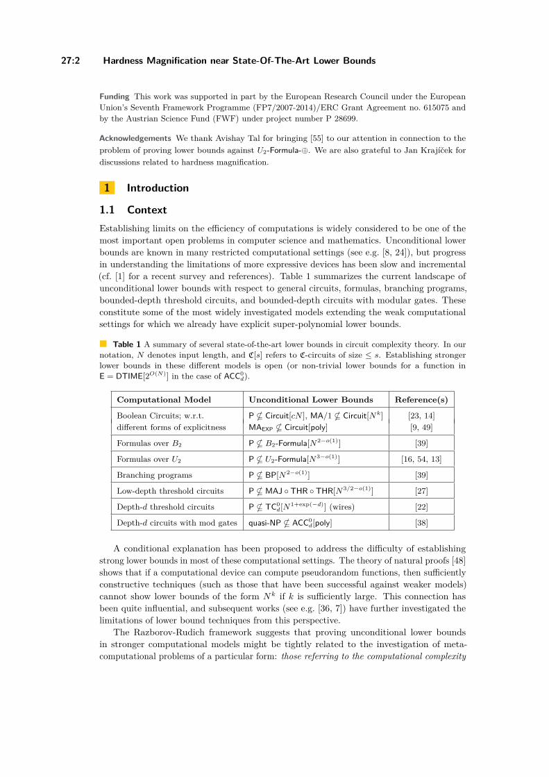
1.1 ContextEstablishing limits on the efficiency of computations is widely considered to be one of themost important open problems in computer science and mathematics. Unconditional lowerbounds are known in many restricted computational settings (see e.g. [8, 24]), but progressin understanding the limitations of more expressive devices has been slow and incremental(cf. [1] for a recent survey and references). Table 1 summarizes the current landscape ofunconditional lower bounds with respect to general circuits, formulas, branching programs,bounded-depth threshold circuits, and bounded-depth circuits with modular gates. Theseconstitute some of the most widely investigated models extending the weak computationalsettings for which we already have explicit super-polynomial lower bounds.

Table 1 A summary of several state-of-the-art lower bounds in circuit complexity theory. In ournotation, N denotes input length, and C[s] refers to C-circuits of size ≤ s. Establishing strongerlower bounds in these different models is open (or non-trivial lower bounds for a function inE = DTIME[2O(N)] in the case of ACC0

d).

Computational Model Unconditional Lower Bounds Reference(s)

Boolean Circuits; w.r.t. P * Circuit[cN ], MA/1 * Circuit[Nk] [23, 14]different forms of explicitness MAEXP * Circuit[poly] [9, 49]

Formulas over B2 P * B2-Formula[N2−o(1)] [39]

Formulas over U2 P * U2-Formula[N3−o(1)] [16, 54, 13]

Branching programs P * BP[N2−o(1)] [39]

Low-depth threshold circuits P * MAJ THR THR[N3/2−o(1)] [27]

Depth-d threshold circuits P * TC0d[N1+exp(−d)] (wires) [22]

Depth-d circuits with mod gates quasi-NP * ACC0d[poly] [38]

A conditional explanation has been proposed to address the difficulty of establishingstrong lower bounds in most of these computational settings. The theory of natural proofs [48]shows that if a computational device can compute pseudorandom functions, then sufficientlyconstructive techniques (such as those that have been successful against weaker models)cannot show lower bounds of the form Nk if k is sufficiently large. This connection hasbeen quite influential, and subsequent works (see e.g. [36, 7]) have further investigated thelimitations of lower bound techniques from this perspective.

The Razborov-Rudich framework suggests that proving unconditional lower boundsin stronger computational models might be tightly related to the investigation of meta-computational problems of a particular form: those referring to the computational complexity

I. C. Oliveira, J. Pich, and R. Santhanam 27:3

of strings or truth-tables. Indeed, it has been subsequently proved that the existence of anatural property for a class of circuits yields explicit lower bounds against the same class[20, 60, 40, 19].

Our results describe a striking phenomenon associated to such problems. They showthat in several scenarios, if we could establish slightly stronger lower bounds for them,i.e., lower bounds that marginally improve the size bounds described in Table 1, thensuper-polynomial lower bounds for explicit problems would follow. More specifically, thisphenomenon concerns computational problems where the complexity of strings are measuredaccording to circuit complexity (often referred to as MCSP; see [26]) or Levin’s time-boundedKolmogorov complexity [32] (a problem known as MKtP; see [5]). MCSP and MKtP areimportant meta-computational problems with connections to areas such as learning theory,cryptography, proof complexity, pseudorandomness and circuit complexity (see e.g. [4] andreferences therein). We refer to [3] for more discussion about the importance of these andrelated complexity measures.

The new results are part of an emerging theory of hardness magnification showing thatweak lower bounds for some problems imply much stronger lower bounds. Several resultsof this form have been obtained in different contexts [52, 6, 33, 37, 41], and we refer to [41]for further discussion. Other forms of hardness magnification are known in settings such ascommunication complexity and arithmetic circuit complexity. A recent example phrased in away that is closer to our results appears in [11] (see also [18]).

As explained in [6, 41], hardness magnification seems to avoid the natural proofs barrierof [48]. It is therefore important to understand the role of magnification in connection tosuper-polynomial lower bounds, and this work takes another step in this direction. Our maincontributions can be informally described as follows:(i) We employ new techniques to obtain the first magnification theorem for the worst-case

formulation of the MCSP problem.1(ii) Our results establish hardness magnification for a natural meta-computational problem

(MKtP) near the lower bound frontiers in several standard circuit models. In addition,we identify a computational model where hardness magnification for MKtP lies belowexisting lower bounds.

(iii) Crucially, our hardness magnification theorems hold for problems for which it is possibleto establish a variety of non-trivial lower bounds.

We believe these results further highlight the relevance of meta-computational problems inconnection to the main open problems in algorithms and complexity theory (see e.g. [59, 12]for recent breakthroughs), and strongly indicate that the investigation of weak lower boundsfor MKtP and MCSP is a fundamental research direction.

1.2 ResultsIn this section, we formally state our results. We also briefly discuss some of our techniques,which are explained in more detail in the main body of the paper. We defer a more elaboratediscussion of some results to Section 1.3.

Notation. We consider formulas over the bases U2 (fan-in two ANDs and ORs), B2 (allboolean functions over two input bits), and extended U2-formulas where the input leavesare labelled by literals, constants, or parity functions over the input bits of arbitrary arity.

1 Independently, Dylan McKay, Cody Murray, and Ryan Williams [35] established a magnification theoremfor a worst-case formulation of MCSP with a completely different proof.

CCC 2019

27:4 Hardness Magnification near State-Of-The-Art Lower Bounds

The corresponding classes of formulas of size at most s (measured by the number of leaves)will be denoted by U2-Formula[s], B2-Formula[s], and U2-Formula-⊕[s], respectively. If we donot specify the type of formulas, we are referring to De Morgan formulas (i.e., formulas overU2). We also consider bounded-depth majority circuits, where each internal gate computes aboolean-valued majority function (MAJ) of the form

∑i∈S yi ≥? t (the circuit has access to

input literals x1, . . . , xn, x1, . . . , xn). We measure the size of such circuits by the number ofwires in the circuit. Depth-d majority circuits of size s will de denoted by MAJ0

d[s], whered ≥ 1 is fixed. We also consider threshold circuits whose internal gates compute a thresholdfunction (THR) of the form

∑i∈S wi · yi ≥? t, for wi, t ∈ R. We count number of gates in this

case, and let TC0d[s] denote the corresponding class of circuits. Circuit[s] denotes fan-in two

boolean circuits of size s and of unbounded depth (gate types do not matter in our results).More generally, for a circuit class C, we use C[s] to denote C-circuits of size ≤ s, where size ismeasured by number of gates. Finally, BP[s] denotes deterministic branching programs ofsize at most s. We refer to a standard textbook (see e.g. [24]) for more information aboutthese boolean devices.

Gap-MKtP and lower bounds for EXP. We use N to denote the input length of an instanceof Gap-MKtP[s1, s2] (see Definition 7 below), where we need to distinguish strings of Ktcomplexity [32] (a certain time-bounded variant of Kolmogorov complexity) at most s1(N)from strings of Kt complexity at least s2(N). It is not hard to see that for constructivebounds s1 < s2, Gap-MKtP[s1, s2] ∈ EXP.

We establish a hardness magnification theorem for Gap-MKtP. (In Section 2, we reviewsome relations between the complexity classes and boolean devices appearing below.) Letn = logN .

I Theorem 1 (Hardness magnification for MKtP). There is a universal constant c ≥ 1 forwhich the following hold. If there exists ε > 0 such that for every small enough β > 01. Gap-MKtP[2βn, 2βn + cn] /∈ Circuit[N1+ε], then EXP * Circuit[poly].2. Gap-MKtP[2βn, 2βn + cn] /∈ U2-Formula-⊕[N1+ε], then EXP * Formula[poly].3. Gap-MKtP[2βn, 2βn + cn] /∈ AND-THR-THR-XOR[N1+ε], then EXP * TC0

2[poly].4. Gap-MKtP[2βn, 2βn + cn] /∈ MAJ0

2d′+d+1[N1+(2/d′)+ε], then EXP * MAJ0d[poly].

5. Gap-MKtP[2βn, 2βn + cn] /∈ B2-Formula[N2+ε], then EXP * Formula[poly].6. Gap-MKtP[2βn, 2βn + cn] /∈ U2-Formula[N3+ε], then EXP * Formula[poly].7. Gap-MKtP[2βn, 2βn + cn] /∈ BP[N2+ε], then EXP * BP[poly].8. Gap-MKtP[2βn, 2βn + cn] /∈ (AC0[6])[N1+ε], then EXP * AC0[6].

Interestingly, this result shows the existence of a single meta-computational problem thatis connected to several frontiers in complexity theory.

The proof of Theorem 1 relies on a refinement of some ideas from [41, Section 3.2]. In fact,item 1 of Theorem 1 is a restatement of [41, Theorem 3]. For a sketch of the argument andits underlying techniques, we refer to the discussion in Section 3. We mention that crucial inthe proof is the use of error-correcting codes, and that the complexity of computing theseobjects using different boolean devices gives rise to the distinct magnification thresholdsobserved in Theorem 1. The formal proof of Theorem 1 appears in Sections 3.1 and 3.2.

In contrast, we observe the following unconditional lower bounds.

I Theorem 2 (Strong lower bounds for large parameters). For every ε > 0 there exists δ > 0for which the following results hold:1. Gap-MKtP[2(1−δ)n, 2n−1] /∈ U2-Formula[N3−ε].2. Gap-MKtP[2(1−δ)n, 2n−1] /∈ B2-Formula[N2−ε].3. Gap-MKtP[2(1−δ)n, 2n−1] /∈ BP[N2−ε].

I. C. Oliveira, J. Pich, and R. Santhanam 27:5

The proof of Theorem 2 is simple, assuming certain results. It relies on the existence ofpseudorandom generators against small formulas and small branching programs [21], togetherwith an observation from [3]. The argument appears in Appendix A.2.

Note the different regime of parameters for Gap-MKtP[s1, s2] in Theorems 1 and 2.In order to magnify a weak lower bound using Theorem 1, we need that it holds fors1 = 2o(n) = No(1). The next result shows that non-trivial unconditional lower bounds canbe obtained in this regime.

I Theorem 3 (A near-quadratic formula lower bound). For every constant 0 < α < 2 thereexists C > 1 such that Gap-MKtP[Cn2, 2(α/2)n−2] /∈ U2-Formula[N2−α].2

The proof of Theorem 3 adapts ideas from [17, Section 4] (see also the exposition in [41,Appendix C.1]) employed in the context of MCSP for larger parameters. A sketch of theargument followed by a proof can be found in Appendix A.1.

Gap-MCSP and lower bounds for NP. We use N = 2n to denote the input length ofan instance of Gap-MCSP[s1, s2] (see Definition 9 below), where one needs to distinguishfunctions of circuit complexity at most s1 from functions of circuit complexity at least s2. Itis not hard to see that for constructive bounds s1 < s2, Gap-MCSP[s1, s2] ∈ NP.

We establish the following magnification theorem for Gap-MCSP.

I Theorem 4 (Hardness magnification for MCSP). There is a universal constant c ≥ 1 forwhich the following holds. If there exists ε > 0 such that for every small enough β > 01. Gap-MCSP[2βn/cn, 2βn] /∈ Circuit[N1+ε], then NP * Circuit[poly].

MCSP and MKtP are quite different problems. In our results, an important distinctionis that applying a polynomial-time function to an input of MKtP does not substantiallyincrease its Kt complexity (cf. Proposition 8), but this is not necessarily true in the contextof circuit complexity, where the input string represents an entire truth-table. For this reason,the proof of Theorem 4 is completely different from the proof of Theorem 1.

Theorem 4 is our main technical contribution. The argument relies on the notion of anti-checkers. Roughly speaking, an anti-checker is a bounded collection S of inputs associatedwith a hard function f such that any small circuit C differs from f on some input in S.More precisely, it was established in [34] that any function f : 0, 1n → 0, 1 that requirescircuits of size s admits a collection Sf containing O(s) strings that is an anti-checker againstcircuits of size roughly s/n. Our argument makes crucial use of anti-checkers, and en routeto Theorem 4 we give a more constructive proof of their existence. (While the proof in [34]uses min-max theory, our proof is combinatorial and self-contained.)

We remark that anti-checkers were first employed for hardness magnification in thecontext of proof complexity [37]. However, while the existential result from [34] was sufficientin that context, this is not the case in circuit complexity, and our argument needs to be moresophisticated. For the reader interested in learning more about hardness magnification inproof complexity, how it relates to meta-computational problems such as MCSP, and howthe new results compare with previous work, we refer to Appendix B.

The proof of Theorem 4 is not difficult given a certain lemma about the constructionof anti-checkers (see Section 4.1). The crucial Anti-Checker Lemma (see Lemma 17) saysthat NP ⊆ Circuit[poly] implies the existence of circuits of almost linear size which given the

2 The constant C has an exponential dependence on 1/α.

CCC 2019

27:6 Hardness Magnification near State-Of-The-Art Lower Bounds

truth table of a Boolean function f print a corresponding set Sf . The circuits provided bythe Anti-Checker Lemma simulate the alternate proof of the existence of anti-checkers, butmake the involved argument constructive by using approximate counting and the assumptionNP ⊆ Circuit[poly]. The strategy for proving the Anti-Checker Lemma is somewhat similar tothe proof of Sp2 ⊆ ZPPNP [10]. A high-level exposition and the complete proof are describedin Section 4.3

I Remark. Implicit in our proof of Theorem 4 is a Turing kernelization for the parameterizedversion of Gap-MCSP which might be of independent interest – there are nearly-linear sizedcircuits which solve any instance of Gap-MCSP with parameter s using oracle access topoly(s)-sized instances of a fixed language in the Polynomial Hierarchy.

We are able to show the following related unconditional lower bound against formulas.

I Theorem 5. For each 0 < α < 2 there exists d > 1 such that Gap-MCSP[nd, 2(α/2−o(1))n] /∈U2-Formula[N2−α].

Consequently, if one could establish an analogue of Theorem 4 for sub-quadratic formulas,then NP * Formula[poly]. We explain why the argument behind the proof of Theorem 4 failsin the case of formulas in Section 4.2.4 The proof of Theorem 5 is similar to the proof ofTheorem 3, and we sketch the necessary modifications in Appendix A.3.

Finally, in Section 4.3 we discuss a certain combinatorial hypothesis (“The Anti-CheckerHypothesis”) connected to the techniques behind the proof of Theorem 4. If this hypothesisholds, then NP * Formula[poly]. We observe that the hypothesis does hold in the average-case, but we are unsure about its plausibility in the worst-case context that is sufficient forsuper-polynomial formula lower bounds.

1.3 DiscussionThis work is a sequel to an earlier paper of two of the authors [41], in which hardnessmagnification was first explored in a systematic way. The results in [41] are for a varietyof problems (including SAT, Vertex Cover and variants of MKtP and MCSP)5 and models(including formulas, circuits and sublinear-time algorithms). For each (problem, model) pairconsidered in [41], it is shown that non-trivial lower bounds for the problem against themodel imply super-polynomial lower bounds for some other explicit problem.

As discussed in [41], there are two natural interpretations of magnification results. Thefirst, more optimistic, interpretation is that magnification constitutes a new approach toproving strong lower bounds. If we are able to replicate the non-trivial circuit lower boundswe can prove against models such as constant-depth circuits (in the worst case) or formulas(in the average case) for the problems witnessing the magnification phenomenon, then thiswould lead to new and powerful lower bounds. There are no well-understood obstaclesto the success of such an approach. In particular, the natural proofs barrier of Razborovand Rudich [48] does not seem to say anything interesting about the success or failure ofsuch an approach.

3 We stress that the assumption that NP ⊆ Circuit[poly] allows several computations to be performedin circuit size O(Nc), where N is the input length. Note however that our requirement is much morestringent: we need to construct anti-checkers using circuits of size O(N1+ε) instead of O(Nc) forsome c ∈ N.

4 Note that Theorem 4 implies lower bounds for a problem in NP. Theorem 1 only gives lower bounds inEXP, but its proof extends to several low-complexity settings.

5 The variant of MCSP investigated in [41] is different than the one discussed in this work, and refers tothe average-case circuit complexity of the input truth table.

I. C. Oliveira, J. Pich, and R. Santhanam 27:7

The other, more pessimistic, interpretation of magnification results is that they indicatethat circuit lower bounds might be even harder to achieve than previously thought. Earlier,super-polynomial lower bounds seemed to be out of reach, but there was no strong reasons tobelieve that small fixed polynomial lower bounds or at least barely non-trivial lower boundsare hard to show. Modulo the belief that super-polynomial circuit lower bounds for explicithard problems are hard to show, the magnification phenomenon suggests that for severalnatural problems of interest, even non-trivial lower bounds are hard to show.

The results of [41] have drawbacks from the point of view of either interpretation, whichthe present work addresses.

For the optimistic interpretation, it would be good to have examples of natural problemswhere some magnification phenomenon holds, and where in addition, there are techniquesgiving non-trivial lower bounds. In this work, we give magnification results for the Gap-MKtPand Gap-MCSP problems, for both of which we show that there are non-trivial lower boundsin the model of Boolean formulas. Thus there is some lower bound technique which works togive a non-trivial result – the question is “merely” whether it can be strengthened to derivea lower bound beyond the magnification threshold.

While the pessimistic interpretation might not lead to new lower bounds, it does havethe potential of leading to a better understanding of barriers. From this point of view, [41] isnot particularly sensitive to the specific model being considered. It is clear that some modelsare easier to prove lower bounds for than others – indeed we have near-cubic lower boundsin the De Morgan formula model, near-quadratic lower bounds in the branching programmodel, and only trivial lower bounds in the Boolean circuit model. Can magnification beused to give a new perspective on these differences between models?

We provide a positive answer to this question, by giving different magnification thresholdsfor different models. What remains mysterious is why known lower bound techniques fallshort of proving lower bounds required to apply magnification. This suggests that there arelimitations of the known techniques above and beyond those captured by natural proofs – animportant direction for further research.

It is worth emphasizing that there are natural problems for which showing lower boundsthat are weaker than the current state-of-the-art size bounds would also imply super-polynomial lower bounds [41]. A representative example presented in [41] concerns anaverage-case version of MCSP, where the problem refers to the average-case circuit complexityof the input function. The reason that work does not imply super-polynomial lower boundsvia magnification is that the corresponding unconditional lower bounds and magnificationtheorems hold for a different regime of the average-case complexity parameter.6

Our results and techniques were motivated in part by the desire to address this gap. Onthe one hand, it seems to be easier to analyse problems that refer to the worst-case complexityof the input. But on the other hand, our new results indicate that the shift from average-caseto worst-case complexity (in the description of the problem) often increases the magnificationthreshold to size bounds that are beyond existing techniques. As a concrete example, ifthe formula magnification theorem for the average-case MCSP problem investigated in [41]could be established for the worst-case variant investigated here, NP * NC1 would followvia Theorem 5. Another glimpse of the subtle transition between worst-case and average-case complexity and its role in magnification appears in the discussion of the Anti-CheckerHypothesis in Section 4.3.

6 In particular, the lower bounds and magnification theorems from [41] do not hold for the same problems.

CCC 2019

27:8 Hardness Magnification near State-Of-The-Art Lower Bounds

Complementing these results, we identify a computational model that has not receivedmuch attention in the literature, and for which the magnification threshold for Gap-MKtPlies below existing lower bounds. This corresponds to Theorem 4 Item 2, i.e., U2-formulasaugmented with parities in the leaves (our exposition in Section 3 focuses on this model).Note that, by a straightforward simulation, before breaking the cubic barrier for U2-formulasor the quadratic barrier for B2-formulas, one needs to show super-linear lower bounds againstU2-Formula-⊕. But a recent result of Tal [55] implies exactly that: the inner product functionover N input bits is not in U2-Formula-⊕[N1.99].

This makes this computational model particularly attractive in connection to hardnessmagnification and lower bounds. Indeed, it seems “obvious” that Gap-MKtP[2δn, 2δn + cn] /∈U2-Formula-⊕[N1.01], given that such formulas cannot compute the much simpler innerproduct function, and that standard formulas require at least near-quadratic size (Theorem 3).Our work shows that if this is the case, then EXP * NC1.

2 Preliminaries

For ` ∈ N, we use [`] to denote the set 1, . . . , `. The length of a string w will be denoted by|w|. Our logarithms are in base 2, and we use exp(x) to denote ex. We use boldface symbolssuch as i and ρ to denote random variables, and x ∈R S to denote that x is a uniformlyrandom element from a set S. We often identify n with logN or N with 2n, depending onthe context.

For concreteness, we employ a random-access model to formalize uniform algorithms. Thedetails of the model are not crucial in our results, and only mildly affect the gap parameterss1 and s2. We fix some standard encoding of algorithms as strings, and use 〈M〉 to denote thestring encoding the algorithm M . Moreover, we assume for simplicity the following propertyof this encoding: if an algorithm C is obtained via the composition of the computations ofalgorithms A and B, then |〈C〉| ≤ |〈A〉|+ |〈B〉|+O(1). (Roughly speaking, composing twocodes gives a new valid code.7) The running time of M on x is denoted by tM (x).

We introduce next the notion of Kt complexity. We adopt a formulation that is moreconvenient for our purposes. In particular, we avoid the use of universal machines in thedefinition given below.8 (Our definition is easily seen to be within at most a logarithmicadditive term of the formulation using universal machines. We stress that our proofs can beadapted to work with any reasonable definition.)

I Definition 6 (Kt Complexity ([32]; see also [3])). For a string x ∈ 0, 1∗, Kt(x) denotesthe minimum of |〈M〉|+ |a|+ dlog tM (a)e over pairs (M,a) such that the machine M outputsx when it computes on the input string a.

I Definition 7 (The Gap-MKtP Problem). We consider the promise problem Gap-MKtP[s1, s2],where s1, s2 : N→ N and s1(N) < s2(N) for all N ∈ N. For each N ≥ 1, Gap-MKtP[s1, s2]

7 While this holds for instance for programs with relative jump instructions (i.e., goto instructions wherethe new line is encoded relative to the number of the current line), we remark this is not true in general.For instance, composing two Turing Machines might require renaming all states of one machine, whichcould result in a new encoding of length (1 + o(1))|〈A〉|+ |〈B〉|. Depending on the computational model,the results in Theorem 1 might need parameters s2 = (1 + o(1))s1.

8 Universal machines are still needed to upper bound the time complexity of computing Kt complexity.Moreover, the exact Kt complexity of a string depends on the choice of encoding for algorithms/machines.

I. C. Oliveira, J. Pich, and R. Santhanam 27:9

is defined by the following sets of instances:

YESNdef= x ∈ 0, 1N | Kt(x) ≤ s1(N) , and

NONdef= x ∈ 0, 1N | Kt(x) > s2(N) .

We will need the following simple result.

I Proposition 8 (Kt complexity and composition). Let B be an algorithm that runs in timeat most TB(N) over inputs of length N . Then, for every input w ∈ 0, 1N , as N growswe have

Kt(B(w)) ≤ Kt(w) + log(TB(N)) +O(1).

Proof. Let A be a machine and a be a string such that the pair (A, a) witnesses the valueKt(w). Let C be the composition of machines A and B, i.e., C(y) = B(A(y)). We claim thatthe pair (C, a) witnesses the inequality in the conclusion of the proposition. Indeed, sinceC(a) = B(A(a)) = B(w), we get

Kt(B(w)) ≤ |〈C〉|+ |a|+ dlog tC(a)e≤ |〈A〉|+ |〈B〉|+O(1) + |a|+ log(tA(a) + tB(w))≤ |〈A〉|+ |a|+ log(tA(a)) + log(tB(w)) + |〈B〉|+O(1)≤ Kt(w) + log(TB(N)) +O(1),

where we have used that |〈B〉| is constant as N grows. J

We also consider a natural formulation of the gap version of the Minimum Circuit SizeProblem (MCSP). The circuit complexity of a boolean function f : 0, 1n → 0, 1 is denotedby Size(f). We use the same notation to represent the circuit complexity of the functionencoded by a string x ∈ 0, 12n .

IDefinition 9 (The Gap-MCSP Problem). We consider the promise problem Gap-MCSP[s1, s2],where s1, s2 : N→ N and s1(n) < s2(n) for all n ∈ N. For each n ≥ 1, Gap-MCSP[s1(n), s2(n)]is defined by the following sets of instances:

YESndef= x ∈ 0, 12n | Size(x) ≤ s1(n) , and

NOndef= x ∈ 0, 12n | Size(x) > s2(n) .

A brief review of uniform complexity classes and connections to non-uniform devices.To provide some context for Theorem 1, we remind the reader about the following relationsinvolving boolean devices and complexity classes. Under an appropriate uniform formulationof circuit classes, we have the inclusions:

(uniform classes) AC0 ⊆ ACC0 ⊆ MAJ0 ⊆ TC0 ⊆ NC1 ⊆ L ⊆ P.

Some of these classes are related in the non-uniform case as follows: NC1 = U2-Formula[poly] =B2-Formula[poly] = (width 5) BP[poly], L/poly = BP[poly], P/poly = Circuit[poly], andMAJ0[poly] = TC0[poly]. These equivalences might require a complexity overhead in size ordepth. We refer to [44, 24] for these and other related results.

CCC 2019

27:10 Hardness Magnification near State-Of-The-Art Lower Bounds

3 Hardness Magnification via Error-Correcting Codes

In this section, we prove Theorem 1. First, we provide a high-level exposition of the argument.

Proof Idea. The result is established in the contrapositive. The idea is to reduce Gap-MKtP[s1, s2] to a problem in EXP over instances of size poly(s1, s2) N , and to invoke theassumed complexity collapse to solve Gap-MKtP using very efficient circuits (or other booleandevices). First, we apply an error-correcting code (ECC) to the input string w ∈ 0, 1N .Since this can be done by a uniform polynomial time computation, we are able to showthat ECC(w) ∈ 0, 1O(N) is a string of Kt complexity ` < s2 if w has Kt complexity ≤ s1.On the other hand, using an efficient decoder for the ECC, we can show that if w has Ktcomplexity ≥ s2, then any string of Kt complexity > ` differs from ECC(w) on a constantfraction of coordinates. Let z = ECC(w). Given the gap in the input instances of Gap-MKtP,our task now is to distinguish strings z that have Kt complexity at most ` from strings thatcannot be approximated by strings of Kt complexity at most `, where s1 < ` < s2.

We achieve this by using a random projection of the input z to a string y of size roughly` N . The intuition is that if z has Kt complexity at most `, then every projection of zalso agrees with some string (i.e., z) of Kt complexity at most `. However, it is possible toargue that if z cannot be approximated by a string of Kt complexity at most `, then withhigh probability no string of Kt complexity at most ` agrees with the randomly projectedcoordinates of z. Checking which case holds when we are given the string y can be done byan exponential time algorithm. Under the assumption that EXP admits small circuits, weare able to solve this problem in complexity poly(`) N .

The reduction sketched above requires (1) the computation of an appropriate ECC, and(2) is randomized. A careful derandomization and the computation of the ECC in differentmodels of computation provide the size bounds corresponding to the magnification thresholdsappearing in the statement of Theorem 1.

We start with a detailed proof of Item (2), which covers the more interesting scenarioof formulas with parity leaves. We then discuss how a simple modification of the argumenttogether with known results imply the other cases.

3.1 Proof of Theorem 1 Case 2 (Magnification for formulas withparities)

We will need the following explicit construction.

I Theorem 10 (Explicit linear error-correcting codes (cf. [25, 50])). There exists a sequenceENN∈N of error-correcting codes EN : 0, 1N → 0, 1M(N) with the following properties:

EN (x) can be computed by a uniform deterministic algorithm running in time poly(N).M(N) = b ·N for a fixed b ≥ 1.There exists a constant δ > 0 such that any codeword EN (x) ∈ 0, 1M(N) that iscorrupted on at most a δ-fraction of coordinates can be uniquely decoded to x by a uniformdeterministic algorithm D running in time poly(M(N)).Each output bit is computed by a parity function: for each input length N ≥ 1 and foreach coordinate i ∈ [M(N)], there exists a set SN,i ⊆ [N ] such that for every x ∈ 0, 1N ,

EN (x)i =⊕j∈SN,i

xj .

I. C. Oliveira, J. Pich, and R. Santhanam 27:11

We proceed with the proof of Theorem 1 Part (2). We establish the contrapositive.Assume that EXP ⊆ Formula[poly], and recall that N = 2n. For any ε > 0, we provethat Gap-MKtP[2βn, 2βn + cn] ∈ U2-Formula-⊕[N1+ε] for a sufficiently small β > 0 and auniversal choice of the constant c. The value of c will be specified later in the proof (seeClaim 12 below).

Let EN : 0, 1N → 0, 1M be the error-correcting code granted by Theorem 10, whereM(N) = bN . Given an instance w ∈ 0, 1N of Gap-MKtP[2βn, 2βn + cn], we first apply ENto w ∈ 0, 1N to get z = EN (w) ∈ 0, 1M .

B Claim 11. There exists c0 ≥ 1 such that for every large enough N the following holds. IfKt(w) ≤ 2βn, then Kt(z) ≤ 2βn + c0n.

Proof. The claim follows immediately from the upper bound on Kt(w), the definition ofz = EN (w), the running time of EN , and Proposition 8. C

B Claim 12. There exist c > c1 > c0 ≥ 1 such that for every large enough N the followingholds. If Kt(w) > 2βn + cn, then Kt(z′) > 2βn + c1n for any z′ ∈ 0, 1M that disagrees withz on at most a δ-fraction of coordinates.

Proof. Suppose that a string z′ ∈ 0, 1M disagrees with z on at most a δ-fraction ofcoordinates, and that Kt(z′) ≤ 2βn + c1n for some c1 > c0. We upper bound the Ktcomplexity of w by combining a description of z′ with the decoder D provided by Theorem10. In more detail, assume the pair (F, a) witnesses Kt(z′). Let B be the machine that firstapplies the machine F to a (producing z′), then D to z′. It follows from Theorem 10 thatB(a) = D(F (a)) = D(z′) = w. Similarly to the proof of Proposition 8, we also get

Kt(w) ≤ |〈B〉|+ |a|+ dlog tB(a)e≤ |〈F 〉|+ |〈D〉|+O(1) + |a|+ log(tF (a) + tD(z′))≤ Kt(z′) + log(tD(z′)) +O(1)≤ (2βn + c1n) +O(n) +O(1)≤ 2βn + cn,

if n is large enough and we choose c sufficiently large. C

Next we define an auxiliary language L ∈ EXP, efficiently reduce Gap-MKtP to L, and usethe assumption that EXP has polynomial size formulas to obtain almost-linear size formulas(of the appropriate kind) for Gap-MKtP. Roughly speaking, we are able to obtain a formulaof non-trivial size for Gap-MKtP because our reduction maps input instances of length N toinstances of L of length No(1) (the o(1) term is captured by the parameter β using n = logN).As we will see shortly, the reduction is randomized. In order to get the final U2-formula-⊕computing Gap-MKtP, the argument is derandomized in a straightforward but careful way.More details follow.

An input string y encoding a tuple (a, 1b, (i1, α1), . . . , (ir, αr)) belongs to L (where a andb are positive integers, a is encoded in binary, and αj ∈ 0, 1) if each ij (for 1 ≤ j ≤ r) is astring of length dlog ae and there is a string z of length a such that Kt(z) ≤ b and for eachindex j we have zij = αj .

B Claim 13. L ∈ EXP.

Proof. L is decidable in exponential time as we can exhaustively search all strings of Ktcomplexity at most b and length exactly a and check if there is one which has the specifiedvalues at the corresponding bit positions. Indeed, using the definition of Kt complexity and

CCC 2019

27:12 Hardness Magnification near State-Of-The-Art Lower Bounds

an efficient universal machine, a list containing all such strings can be generated in timepoly(2b), which is at most exponential in the input length 1b. In turn, checking that a stringof length a satisfies the requirement takes time at most exponential in the total input length,since each index ij is a string of length dlog ae. C

Since EXP ⊆ Formula[poly] by assumption, L has polynomial-size formulas. Assumewithout loss of generality that L has formulas of size O(`k) for some constant k, where ` isits total input length. We choose β = ε/100k.

We are ready to describe a low-complexity reduction from Gap-MKtP[2βn, 2βn + cn] to L.First, we use the error-correcting code to compute z from w, as described above. Then weapply the following sampling procedure. We sample uniformly and independently r = 22βn

indices i1, . . . , ir ∈R [M ], where M = bN . We then form the string y encoding the tuple

(M, 12βn+c1n, (i1, zi1), . . . , (ir, zir )),

where c1 > c0 ≥ 1 is provided by Claim 12. Note that this is a string of length `(N) ≤ Nε/10k.

B Claim 14. The following implications hold:(a) If w ∈ 0, 1N is a positive instance of Gap-MKtP[2βn, 2βn + cn], then y ∈ L with

probability 1.(b) If w ∈ 0, 1N is a negative instance of Gap-MKtP[2βn, 2βn + cn], then y /∈ L with

probability > 1/2.

Proof. If w is a YES instance, we have by Claim 11 that Kt(z) ≤ 2βn + c0n ≤ 2βn + c1n. Inthis case, z is a string of length M that has the specified values at the specified bit positions,regardless of the random positions that are sampled by the reduction. Consequently, y ∈ Lwith probability 1.

For the claim about NO instances, as previously established in Claim 12, we have thatKt(z′) > 2βn + c1n for any z′ such that |z′| = |z| = M and Pri∈R[M ][z′i 6= zi] ≤ δ. Nowconsider any string z′′ of length M such that Kt(z′′) ≤ 2βn + c1n. For such a string z′′, foreach j ∈ [r], the probability that the random projection satisfies z′′ij

= zij(where ij ∈R [M ])

is at most 1− δ. Hence the probability that z′′ agrees with z at all the specified bit positionsis at most (1− δ)r ≤ exp(−δr) ≤ exp(−δ22βn). By a union bound over all strings z′′ withKt(z′′) ≤ 2βn + c1n, the probability that there exists a string z′′ with Kt complexity at most2βn + c1n which is consistent with the values at the specified bit positions is exponentiallysmall in n. Hence with high probability y /∈ L. C

To sum up, there is a randomized reduction from Gap-MKtP[2βn, 2βn + cn] over inputs oflength N to instances of L of length `(N) ≤ Nε/10k. Now let F`(N)N≥1 be a sequence of U2-formulas of size O(`k) for L. Our randomized formulasG(·) for Gap-MKtP compute as follows.

1. G(w) =∧Nj=1G

(j)(w), where each G(j) is an independent copy.2. EachG(j)(w) is a randomized formula of the form G(j)(w, i1, . . . , ir) that first computes z

from w, then computes y from z using the (random) input indices i1, . . . , ir ∈ 0, 1logM ,and finally applies F` to y.

It follows from Claim 14 using the independence of each G(j) that

Pr[G(w) is incorrect ] < 2−N ,

where the probability is taken over the choice of the random input of G. Consequently, by aunion bound there is a fixed choice γ ∈ 0, 1∗ of the randomness of G (corresponding tothe positions of the different random projections) such that the deterministic formula Gγobtained from G and γ is correct on every input string w.

I. C. Oliveira, J. Pich, and R. Santhanam 27:13

B Claim 15. Each deterministic sub-formula G(j)γ (w) can be computed by a U2-formula

extended with parities at the leaves of size at most O(`(N)k) ≤ Nε/2.

Proof. Note that each bit of z can be computed from the input string w using an appropriateparity function (as described in Theorem 10). We argue that the leaves of G(j)

γ are preciselythe leaves of the U2-formula F` replaced by appropriate literals, constants, or parities. Recallthat G(j)

γ applies F` to the string y obtained from z. However, since γ is fixed, the positionsof z that are projected in order to compute y are also fixed, and so are the substrings of ydescribing the corresponding positions. Consequently, the size (i.e. number of leaves) of eachG

(j)γ is at most the size of F`, which proves the claim. C

It follows from this claim that Gγ(w) can be computed by a formula containing at mostN1+ε leaves, and hence Gap-MKtP[2βn, 2βn + cn] ∈ U2-Formula-⊕[N1+ε]. (Observe that wehave used in a crucial way that the derandomized sub-formulas do not need to computeaddress functions to generate y from z.) This completes the proof of Theorem 1 Part (2).

3.2 Completing the proof of Theorem 1In this section, we discuss how the argument presented in Section 3.1 can be adapted toestablish the remaining items of Theorem 1.

First, note that Items (5) and (6) immediately follow from Item (2). This is because aparity gate over at most N input variables can be computed by B2-formulas of size O(N) andby U2-formulas of size O(N2). Consequently, using that formula size is measured with respectto the number of leaves, we immediately get U2-Formula-⊕[s(N)] ⊆ B2-Formula[s(N) · N ]and U2-Formula-⊕[s(N)] ⊆ U2-Formula[s(N) ·N2].

In order to get Item (1), it is sufficient to compute an error-correcting code as in Theorem10 using circuits of (almost) linear size. In other words, we need the entire codeword (andnot just each output bit) to be computable from the input message using a circuit of sizeO(N). The existence of such codes is well-known [50, 51]. The rest of the reduction producesan additive overhead in circuit size of at most N1+ε gates.

Finally, to establish Item (4), we use the following construction from [56].

I Theorem 16 (Computing ECCs in parallel using majorities and few wires [56]). For everydepth d′ ≥ 1 there are constants δ(d′) > 0 and b(d′) ≥ 1 and a sequence ENN∈N oferror-correcting codes EN : 0, 1N → 0, 1M with the following properties:

EN (x) can be computed by a uniform deterministic algorithm running in time poly(N).M(N) = b ·N .Any codeword EN (x) ∈ 0, 1M that is corrupted on at most a δ-fraction of coordinatescan be uniquely decoded to x by a uniform deterministic algorithm D running in timepoly(M).EN (x) ∈ 0, 1M can be computed by a multi-output circuit from MAJ0

2d′ [O(N1+(2/d′))],where circuit size is measured by number of wires.

Following the steps of the reduction described in Section 3.1, under the assumption thatEXP ⊆ MAJ0

d[poly] the final depth of the circuit solving Gap-MKtP is 2d′ + d+ 1, where theterms in this sum correspond respectively to the computation of the error-correcting code(for a choice of d′ ≥ 1), each (circuit) G(j)

α , and the topmost AND gate in Gα (constant bitscan be produced in depth 1 from input literals). Similarly, the overall size (number of wires)of the circuit is O(N1+(2/d′)) +O(N1+ε) +O(N) ≤ N1+(2/d′)+ε.

Item (3) is established in the obvious way given the previous explanations. Item (8) usesthat parity gates can be simulated using mod 6 gates.

CCC 2019

27:14 Hardness Magnification near State-Of-The-Art Lower Bounds

Finally, we deal with case (7), which refers to branching program complexity. First,note that the parity of n bits can be computed by a branching program of size O(n). Inaddition, if f(x) = g(h1(x), . . . , hk(x)), each hi has a branching program of size s, and g hasa branching program of size t, then f has a branching program of size ` = O(t · s). Finally, aconjunction of N branching programs of size ` has branching program size at most O(N · `).Combining these facts in the natural way yields case (7). This completes the proof of allcases in Theorem 1.

4 Hardness Magnification via Anti-Checkers

4.1 Proof of Theorem 4 (Magnification for MCSP)In this section, we derive Theorem 4 from Lemma 17, whose proof appears in Section 4.2.Informally, an anti-checker (cf. [34]) for a function f is a multi-set of input strings such thatany circuit of bounded size that does not compute f is incorrect on at least one of thesestrings.

I Lemma 17 (Anti-Checker Lemma). If NP ⊆ Circuit[poly] there is a constant k ∈ N forwhich the following hold. For every sufficiently small β > 0, there is a circuit C of size≤ 2n+kβn that when given as input a truth-table tt(f) ∈ 0, 1N , where f : 0, 1n → 0, 1,outputs t = 210βn strings y1, . . . , yt ∈ 0, 1n such that if f /∈ Circuit[2βn] then every circuitof size ≤ s where s = 2βn/10n fails to compute f on at least one of these strings.

The Anti-Checker Lemma is a powerful tool that might be of independent interest. Itsays that anti-checkers of bounded size for functions requiring circuits of size 2o(n) can beproduced in time that is almost-linear in the size of the function (viewed as a string), underthe assumption that circuit lower bounds do not hold.9

Proof of Theorem 4. Assume that NP ⊆ Circuit[poly]. We prove that for every given ε > 0there exists a small enough β > 0 such that Gap-MCSP[2βn/10n, 2βn] ∈ Circuit[N1+ε].

We consider the problem Succinct-MCSP, defined next. Its input instances are of the form〈1n, 1s, 1t, (x1, b1), . . . , (xt, bt)〉, where xi ∈ 0, 1n and bi ∈ 0, 1, i ∈ [t]. Note that eachinstance can be encoded by a string of length exactly m = n+ 1 + s+ 1 + t+ 1 + t · (n+ 1).An input string is a positive instance if and only if it is in the appropriate format andthere exists a circuit D over n input variables and of size at most s such that D(xi) = bifor all i ∈ [t]. Note that the problem is in NP as a function of its total input length m.Under the assumption that NP is easy for non-uniform circuits, there exists ` ∈ N suchthat Succinct-MCSP can be solved by circuits Em of size m` on every large enough inputlength m.

Take β = ε/(100 · ` · k), where k is the constant from Lemma 17. In order to constructa circuit for Gap-MCSP, first we reduce this problem to an instance of Succinct-MCSP oflength m using Lemma 17, then we invoke the ml-sized circuit for this problem. Moreprecisely, on an input f : 0, 1n → 0, 1, we use the circuit C (as in Lemma 17) toproduce a list of strings y1, . . . , yt ∈ 0, 1n, generate from this list and f the input instancez = 〈1n, 1s, 1t, ((y1, f(y1)), . . . , (yt, f(yt))〉, for parameters s = 2βn/10n, t = 210βn, m =poly(n) · 210βn, and output Em(z).

9 We have made no attempt to optimize the constants in Lemma 17.

I. C. Oliveira, J. Pich, and R. Santhanam 27:15

Correctness follows immediately from Lemma 17 and our choice of parameters. Indeed, iff ∈ Circuit[2βn/10n] then no matter the choice of y1, . . . , yt the circuit Em accepts z thanksto our choice of s = 2βn/10n. On the other hand, when f /∈ Circuit[2βn] then by Lemma 17every circuit of size s fails on some string from the list, and consequently Em(z) = 0.

We upper bound the total circuit size using the choice of β. Circuit C has size at most2n+kβn ≤ N1+ε/3. In addition, producing the input z can be done from f and y1, . . . , yt bya circuit of size at most O(t ·N) ≤ N1+ε/3, since each address function can be computedin linear size O(N) (see e.g. [58]). Finally, Em has size at most m` ≤ N1+ε/3. Overall, itfollows that Gap-MCSP[2βn/10n, 2βn] is computable by circuits of size N1+ε. J

4.2 Proof of Lemma 17 (Anti-Checker Lemma)This section is dedicated to the proof of Lemma 17. This completes the proof of Theorem 4.We start with a high-level exposition of the argument.

Proof Idea. We take β → 0, for simplicity of the exposition. In principle, the challengeis to construct the list of strings from the description of f using a circuit of size N1+o(1),given that the existence of such strings is guaranteed by the work of [34]. But it is notclear how to use this existential result and the assumption that NP has polynomial sizecircuits to construct almost-linear size circuits for this task. In order to achieve this, we usea self-contained argument that produces the strings one by one until very few circuits ofbounded size are consistent with the values of f on the partial list of strings. We then findpolynomially many additional strings that eliminate the remaining circuits, completing thelist of strings.10

To produce the i-th string yi ∈ 0, 1n given y1, . . . , yi−1 ∈ 0, 1n and f , we estimatethe number of circuits of size ≤ 2βn/10n that agree with f over all strings in y1, . . . , yi.We show that some string yi will reduce the number of consistent circuits from the previousround by a factor of (roughly) 1−1/n if there are at least (roughly) n2 surviving circuits (thisis a combinatorial existential proof that relies on the lower bound on the circuit complexityof f). As a consequence, it will be possible to show that at most 2O(βn) = No(1) roundssuffice to produce the required set of strings (modulo handling the few surviving circuits).The existence of a good string yi is at the heart of our argument, and we defer the expositionof this result to the formal proof.

In each round, we exhaustively check each of the N candidate strings yi. As we willexplain soon, estimating the number of surviving circuits after picking a new candidate stringyi can be done by a circuit of size No(1) given access to y1, . . . , yi and to the correspondingbits f(y1), . . . , f(yi).11 In summary, there are No(1) rounds, and in each one of them wecan find a good string yi using a circuit of size N1+o(1). We remark that it will also bepossible to produce the additional strings in circuit complexity No(1), so that the completelist y1, . . . , yt can be computed from f by a circuit of size N1+o(1).

It remains to explain how to fix a good string in each round. We simply pick the mostpromising string, using that we can upper bound the complexity of estimating the number ofsurviving circuits. The latter relies on the assumed inclusion NP ⊆ Circuit[poly]. Indeed, from

10 In particular, our argument implies the worst-case version of the anti-checker result from [34] withslightly different parameters.

11Technically speaking, projecting f(yi) ∈ 0, 1 from the input string f ∈ 0, 1N and the addressy ∈ 0, 1n already takes circuit complexity Ω(N). However, since we are trying all possible strings yi,the corresponding bit positions of f can be directly hardwired.

CCC 2019

27:16 Hardness Magnification near State-Of-The-Art Lower Bounds

this assumption it follows that the polynomial hierarchy PH ⊆ Circuit[poly], and it is knownthat relative approximate counting can be done in the polynomial hierarchy.12 Crucially, asdescribed in the paragraph above, the input length of each sub-problem that we need tosolve is ≤ No(1) (using that i is at most No(1)), so a polynomial overhead will not be anissue when solving a sub-task of input length No(1). This completes the sketch of the proof.

We proceed with a formal proof of Lemma 17. Let R be a polynomial-time relation, whereR ⊆

⋃m0, 1m × 0, 1q(m) for some polynomial q. For every x, we use R#(x) to denote

|y ∈ 0, 1q(|x|) : (x, y) ∈ R|. A randomized algorithm Π is called an (ε, δ)-approximatorfor R if for every input x it holds that

Pr[ ∣∣Π(x)−R#(x)

∣∣ ≥ ε(|x|) ·R#(x)]≤ δ(|x|).

I Theorem 18 (Relative approximate counting in BPPNP ([53]; see e.g. [15, Section 6.2.2])).For every polynomial-time relation R and every polynomial p, there exists a probabilisticpolynomial-time algorithm A with access to a SAT oracle that is an (1/p(m), 2−p(m))-approximator for R over inputs x of length m.

I Corollary 19. Assume NP ⊆ Circuit[poly]. For every polynomial-time relation R and foreach m ≥ 1, there is a multi-output circuit CR : 0, 1m → 0, 1poly(m) of polynomial sizesuch that on every input x ∈ 0, 1m,

(1− 1/m2) ·R#(x) ≤ CR(x) ≤ (1 + 1/m2) ·R#(x).

Proof. This follows from Theorem 18 (using p(m) = m2) by non-uniformly fixing therandomness of the algorithm, replacing the SAT oracle using the assumption that NP hassmall circuits, and translating the resulting deterministic algorithm into a boolean circuit. J

We define a relation Q. The first input x is of the form 〈1n, 1s, 1i, 1t, (z1, b1), . . . , (zi, bi)〉,where zj ∈ 0, 1n and bj ∈ 0, 1 for 1 ≤ j ≤ i, and t = 210βn (t is used here to pad theinput appropriately). The second input is a string w of length m1/5 (for m = |x|) that isinterpreted as a boolean circuit Cw over n input variables and of size at most s. We let(x,w) ∈ Q if and only if Cw(zj) = bj for all j ∈ [i]. Note that Q is a polynomial-time relation.

We employ circuits obtained from Corollary 19 using parameters s = 2βn/10n and1 ≤ i ≤ t, where t = 210βn. The following result is immediate from Corollary 19 given thatfor our choice of parameters m = poly(2βn).

I Proposition 20 (Circuits for approximate counting). There is a constant k1 ∈ N for whichthe following holds. For every n ≥ 1, let s = 2βn/10n, t = 210βn, 1 ≤ i ≤ t. Then there is amulti-output circuit Cn,i of size ≤ 2k1βn that outputs ≤ 2k1βn bits such that on every inputa = ((z1, b1), . . . , (zi, bi)) ∈ 0, 1i·(n+1),

(1− 1/n10) ·Q#(x) ≤ Cn,i(a) ≤ (1 + 1/n10) ·Q#(x),

where x = x(a) is defined from the string a and from our choice of parameters in theobvious way.

The next step is to guarantee that once just a few circuits remain consistent with f overour partial list of strings (as described in the proof sketch above), we can efficiently find asmall number of strings to eliminate all of them.

12 In our formal proof, we take a slightly more direct route to compute the relative approximations.

I. C. Oliveira, J. Pich, and R. Santhanam 27:17

I Lemma 21 (Listing the remaining circuits). Assume NP ⊆ Circuit[poly]. There exists aconstant k2 ∈ N for which the following holds. Let a = ((z1, b1), . . . , (zt′ , bt′)), where t′ ≤ t,and x = x(a) be the corresponding input of Q. There is a circuit Dn,t′ of size ≤ 2k2βn suchthat if Q#(x) ≤ n3, then Dn,t′(a) outputs a string describing all such circuits.

Proof. It follows from NP ⊆ Circuit[poly] using a standard argument that PH ⊆ Circuit[poly].In addition, it is not hard to define a relation in PH (using a padded input containing thestring 1t) that checks if a given input a satisfies Q#(x(a)) ≤ n3. Consequently, checking if astring λ describes a list of such circuits for a can be done by a circuit of size at most poly(t).Using again that NP ⊆ Circuit[poly] and a self-reduction, we obtain circuits Dn,t′ as in thestatement of the lemma. J

I Lemma 22 (Completing the list of strings). There is a constant k3 ∈ N for which thefollowing holds. For every n ≥ 1 there is a circuit En of size ≤ 2n+k3βn that given accessto a truth-table f ∈ 0, 12n and a string w ∈ 0, 12βn describing a circuit Cw of sizes ≤ 2βn/10n that does not compute f , En(f, w) outputs a string y such that C(y) 6= f(y).

Proof. First, En evaluates Cw on every string z ∈ 0, 1n. This can be easily done by acircuit of size 2n · poly(|w|) under a reasonable encoding of the circuit Cw. Then En inspectsone-by-one each string z and stores the first string where Cw and f differ. Note that a circuitof size ≤ 2n · poly(n) can print this string from the truth-table of f and Cw. It follows thatthe overall complexity of En is 2n+k3βn for some constant k3. J

The previously established results will allow us to find in each round a string yi thatsignificantly reduces the number of remaining circuits (while at least one such string exists),and then to complete the list so that no circuit of bounded size is consistent with all stringsin the final list. We show next that if f is hard and a reasonable number of circuits ofbounded size are consistent with the current list of strings, then a good string yi exists.

For convenience, we introduce a function to capture the fraction of strings encodingcircuits that are consistent with a set of inputs and their corresponding labels. Givena = ((z1, b1), . . . , (zi, bi)), let x = x(a) be the corresponding input to Q under our choice ofparameters. Furthermore, let m = |x|, and recall that Q ⊆

⋃m≥10, 1m × 0, 1m

1/5 . Inorder to maintain the same underlying domain size when considering the fraction of consistentcircuits, we assume without loss of generality using appropriate padding that the encoding ofx has a fixed length m = m(n) for each choice of n (i.e., the choice of 1 ≤ i ≤ t does not affectm1/5). In addition, we can take m(n) ≤ 211βn, which will be useful when upper bounding thenumber of necessary rounds. We let φ(a) ∈ [0, 1] denote the ratio Q#(x(a))/2m1/5 . (Thus inour formal argument we count circuits using their descriptions as binary strings.)

I Lemma 23 (Existence of a good string yi). For every integer i ≥ 1 and for everyz1, . . . , zi−1 ∈ 0, 1n, let a = ((z1, f(z1)), . . . , (zi−1, f(zi−1))). If

f /∈ Circuit[2βn] and Q#(x(a)) ≥ 4n2,

then there is some string yi ∈ 0, 1n such that if a′ denotes the sequence a augmented with(yi, f(yi)), then

φ(a′) ≤ φ(a) · (1− 1/2n).

Proof. The argument is inspired by a combinatorial principle discussed in [29]. Considerthe tuple a and the string x = x(a) as in the statement of the lemma. Moreover, letQ(x) = w ∈ 0, 1m1/5 : (x,w) ∈ Q. For convenience, let r = |Q(x)| = Q#(x) ≥ 4n2, using

CCC 2019

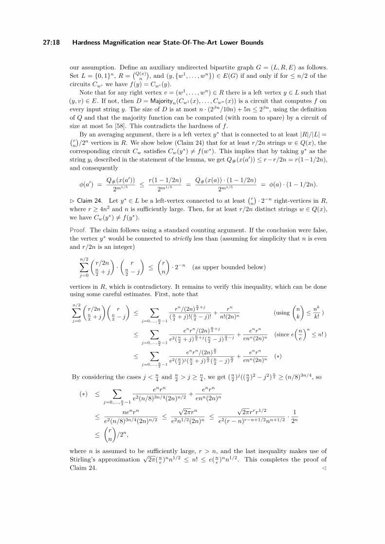
27:18 Hardness Magnification near State-Of-The-Art Lower Bounds

our assumption. Define an auxiliary undirected bipartite graph G = (L,R,E) as follows.Set L = 0, 1n, R =

(Q(x)n

), and (y, w1, . . . , wn) ∈ E(G) if and only if for ≤ n/2 of the

circuits Cwi we have f(y) = Cwi(y).Note that for any right vertex v = (w1, . . . , wn) ∈ R there is a left vertex y ∈ L such that

(y, v) ∈ E. If not, then D = Majorityn(Cw1(x), . . . , Cwn(x)) is a circuit that computes f onevery input string y. The size of D is at most n · (2βn/10n) + 5n ≤ 2βn, using the definitionof Q and that the majority function can be computed (with room to spare) by a circuit ofsize at most 5n [58]. This contradicts the hardness of f .

By an averaging argument, there is a left vertex y∗ that is connected to at least |R|/|L| =(rn

)/2n vertices in R. We show below (Claim 24) that for at least r/2n strings w ∈ Q(x), the

corresponding circuit Cw satisfies Cw(y∗) 6= f(w∗). This implies that by taking y∗ as thestring yi described in the statement of the lemma, we get Q#(x(a′)) ≤ r−r/2n = r(1−1/2n),and consequently

φ(a′) = Q#(x(a′))2m1/5 ≤ r(1− 1/2n)

2m1/5 = Q#(x(a)) · (1− 1/2n)2m1/5 = φ(a) · (1− 1/2n).

B Claim 24. Let y∗ ∈ L be a left-vertex connected to at least(rn

)· 2−n right-vertices in R,

where r ≥ 4n2 and n is sufficiently large. Then, for at least r/2n distinct strings w ∈ Q(x),we have Cw(y∗) 6= f(y∗).

Proof. The claim follows using a standard counting argument. If the conclusion were false,the vertex y∗ would be connected to strictly less than (assuming for simplicity that n is evenand r/2n is an integer)

n/2∑j=0

(r/2nn2 + j

)·(

rn2 − j

)≤(r

n

)· 2−n (as upper bounded below)

vertices in R, which is contradictory. It remains to verify this inequality, which can be doneusing some careful estimates. First, note thatn/2∑j=0

(r/2nn2 + j

)(r

n2 − j

)≤

∑j=0,...,n2 −1

rn/(2n)n2 +j

(n2 + j)!(n2 − j)!+ rn

n!(2n)n (using(n

k

)≤ nk

k! )

≤∑

j=0,...,n2 −1

enrn/(2n)n2 +j

e2(n2 + j)n2 +j(n2 − j)n2 −j + enrn

enn(2n)n (since e(n

e

)n≤ n! )

≤∑

j=0,...,n2 −1

enrn/(2n)n2e2(n2 )j(n2 + j)n2 (n2 − j)

n2

+ enrn

enn(2n)n (∗)

By considering the cases j < n4 and n

2 > j ≥ n4 , we get (n2 )j((n2 )2 − j2)n2 ≥ (n/8)3n/4, so

(∗) ≤∑

j=0,...,n2−1

enrn

e2(n/8)3n/4(2n)n/2 + enrn

enn(2n)n

≤ nenrn

e2(n/8)3n/4(2n)n/2 ≤√

2πrn

e2n1/2(2n)n≤

√2πrrr1/2

e2(r − n)r−n+1/2nn+1/2 ·12n

≤(r

n

)/2n,

where n is assumed to be sufficiently large, r > n, and the last inequality makes use ofStirling’s approximation

√2π(ne )nn1/2 ≤ n! ≤ e(ne )nn1/2. This completes the proof of

Claim 24. C

I. C. Oliveira, J. Pich, and R. Santhanam 27:19

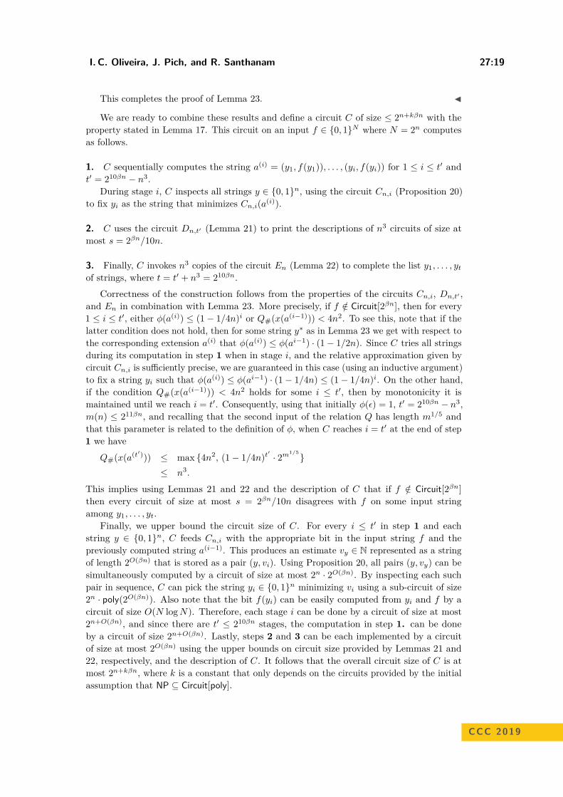
This completes the proof of Lemma 23. J

We are ready to combine these results and define a circuit C of size ≤ 2n+kβn with theproperty stated in Lemma 17. This circuit on an input f ∈ 0, 1N where N = 2n computesas follows.

1. C sequentially computes the string a(i) = (y1, f(y1)), . . . , (yi, f(yi)) for 1 ≤ i ≤ t′ andt′ = 210βn − n3.

During stage i, C inspects all strings y ∈ 0, 1n, using the circuit Cn,i (Proposition 20)to fix yi as the string that minimizes Cn,i(a(i)).

2. C uses the circuit Dn,t′ (Lemma 21) to print the descriptions of n3 circuits of size atmost s = 2βn/10n.

3. Finally, C invokes n3 copies of the circuit En (Lemma 22) to complete the list y1, . . . , ytof strings, where t = t′ + n3 = 210βn.

Correctness of the construction follows from the properties of the circuits Cn,i, Dn,t′ ,and En in combination with Lemma 23. More precisely, if f /∈ Circuit[2βn], then for every1 ≤ i ≤ t′, either φ(a(i)) ≤ (1− 1/4n)i or Q#(x(a(i−1))) < 4n2. To see this, note that if thelatter condition does not hold, then for some string y∗ as in Lemma 23 we get with respect tothe corresponding extension a(i) that φ(a(i)) ≤ φ(ai−1) · (1− 1/2n). Since C tries all stringsduring its computation in step 1 when in stage i, and the relative approximation given bycircuit Cn,i is sufficiently precise, we are guaranteed in this case (using an inductive argument)to fix a string yi such that φ(a(i)) ≤ φ(ai−1) · (1− 1/4n) ≤ (1− 1/4n)i. On the other hand,if the condition Q#(x(a(i−1))) < 4n2 holds for some i ≤ t′, then by monotonicity it ismaintained until we reach i = t′. Consequently, using that initially φ(ε) = 1, t′ = 210βn − n3,m(n) ≤ 211βn, and recalling that the second input of the relation Q has length m1/5 andthat this parameter is related to the definition of φ, when C reaches i = t′ at the end of step1 we have

Q#(x(a(t′))) ≤ max 4n2, (1− 1/4n)t′· 2m

1/5

≤ n3.

This implies using Lemmas 21 and 22 and the description of C that if f /∈ Circuit[2βn]then every circuit of size at most s = 2βn/10n disagrees with f on some input stringamong y1, . . . , yt.

Finally, we upper bound the circuit size of C. For every i ≤ t′ in step 1 and eachstring y ∈ 0, 1n, C feeds Cn,i with the appropriate bit in the input string f and thepreviously computed string a(i−1). This produces an estimate vy ∈ N represented as a stringof length 2O(βn) that is stored as a pair (y, vi). Using Proposition 20, all pairs (y, vy) can besimultaneously computed by a circuit of size at most 2n · 2O(βn). By inspecting each suchpair in sequence, C can pick the string yi ∈ 0, 1n minimizing vi using a sub-circuit of size2n · poly(2O(βn)). Also note that the bit f(yi) can be easily computed from yi and f by acircuit of size O(N logN). Therefore, each stage i can be done by a circuit of size at most2n+O(βn), and since there are t′ ≤ 210βn stages, the computation in step 1. can be doneby a circuit of size 2n+O(βn). Lastly, steps 2 and 3 can be each implemented by a circuitof size at most 2O(βn) using the upper bounds on circuit size provided by Lemmas 21 and22, respectively, and the description of C. It follows that the overall circuit size of C is atmost 2n+kβn, where k is a constant that only depends on the circuits provided by the initialassumption that NP ⊆ Circuit[poly].

CCC 2019

27:20 Hardness Magnification near State-Of-The-Art Lower Bounds

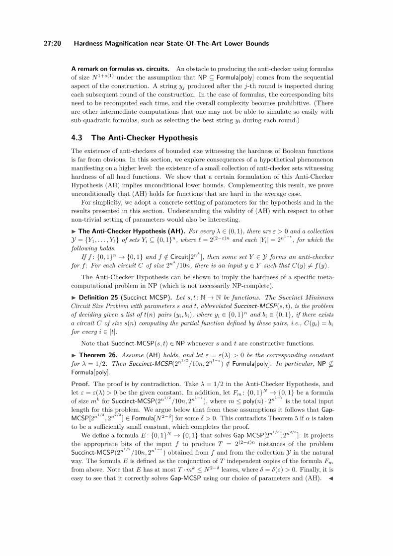
A remark on formulas vs. circuits. An obstacle to producing the anti-checker using formulasof size N1+o(1) under the assumption that NP ⊆ Formula[poly] comes from the sequentialaspect of the construction. A string yj produced after the j-th round is inspected duringeach subsequent round of the construction. In the case of formulas, the corresponding bitsneed to be recomputed each time, and the overall complexity becomes prohibitive. (Thereare other intermediate computations that one may not be able to simulate so easily withsub-quadratic formulas, such as selecting the best string yi during each round.)

4.3 The Anti-Checker HypothesisThe existence of anti-checkers of bounded size witnessing the hardness of Boolean functionsis far from obvious. In this section, we explore consequences of a hypothetical phenomenonmanifesting on a higher level: the existence of a small collection of anti-checker sets witnessinghardness of all hard functions. We show that a certain formulation of this Anti-CheckerHypothesis (AH) implies unconditional lower bounds. Complementing this result, we proveunconditionally that (AH) holds for functions that are hard in the average case.

For simplicity, we adopt a concrete setting of parameters for the hypothesis and in theresults presented in this section. Understanding the validity of (AH) with respect to othernon-trivial setting of parameters would also be interesting.

I The Anti-Checker Hypothesis (AH). For every λ ∈ (0, 1), there are ε > 0 and a collectionY = Y1, . . . , Y` of sets Yi ⊆ 0, 1n, where ` = 2(2−ε)n and each |Yi| = 2n1−ε , for which thefollowing holds.

If f : 0, 1n → 0, 1 and f /∈ Circuit[2nλ ], then some set Y ∈ Y forms an anti-checkerfor f : For each circuit C of size 2nλ/10n, there is an input y ∈ Y such that C(y) 6= f(y).

The Anti-Checker Hypothesis can be shown to imply the hardness of a specific meta-computational problem in NP (which is not necessarily NP-complete).

I Definition 25 (Succinct MCSP). Let s, t : N → N be functions. The Succinct MinimumCircuit Size Problem with parameters s and t, abbreviated Succinct-MCSP(s, t), is the problemof deciding given a list of t(n) pairs (yi, bi), where yi ∈ 0, 1n and bi ∈ 0, 1, if there existsa circuit C of size s(n) computing the partial function defined by these pairs, i.e., C(yi) = bifor every i ∈ [t].

Note that Succinct-MCSP(s, t) ∈ NP whenever s and t are constructive functions.

I Theorem 26. Assume (AH) holds, and let ε = ε(λ) > 0 be the corresponding constantfor λ = 1/2. Then Succinct-MCSP(2n1/2

/10n, 2n1−ε) /∈ Formula[poly]. In particular, NP *Formula[poly].

Proof. The proof is by contradiction. Take λ = 1/2 in the Anti-Checker Hypothesis, andlet ε = ε(λ) > 0 be the given constant. In addition, let Fm : 0, 1N → 0, 1 be a formulaof size mk for Succinct-MCSP(2n1/2

/10n, 2n1−ε), where m ≤ poly(n) · 2n1−ε is the total inputlength for this problem. We argue below that from these assumptions it follows that Gap-MCSP[2n1/3

, 2n2/3 ] ∈ Formula[N2−δ] for some δ > 0. This contradicts Theorem 5 if α is takento be a sufficiently small constant, which completes the proof.

We define a formula E : 0, 1N → 0, 1 that solves Gap-MCSP[2n1/3, 2n2/3 ]. It projects

the appropriate bits of the input f to produce T = 2(2−ε)n instances of the problemSuccinct-MCSP(2n1/2

/10n, 2n1−ε) obtained from f and from the collection Y in the naturalway. The formula E is defined as the conjunction of T independent copies of the formula Fmfrom above. Note that E has at most T ·mk ≤ N2−δ leaves, where δ = δ(ε) > 0. Finally, it iseasy to see that it correctly solves Gap-MCSP using our choice of parameters and (AH). J

I. C. Oliveira, J. Pich, and R. Santhanam 27:21

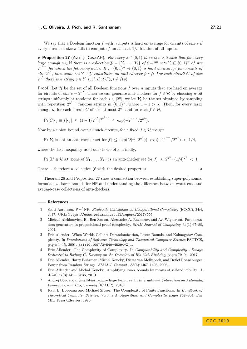
We say that a Boolean function f with n inputs is hard on average for circuits of size s ifevery circuit of size s fails to compute f on at least 1/s fraction of all inputs.

I Proposition 27 (Average-Case AH). For every λ ∈ (0, 1) there is ε > 0 such that for everylarge enough n ∈ N there is a collection Y = Y1, . . . , Y` of ` = 2n sets Yi ⊆ 0, 1n of size2n1−ε for which the following holds. If f : 0, 1n → 0, 1 is hard on average for circuits ofsize 2nλ , then some set Y ∈ Y constitutes an anti-checker for f : For each circuit C of size2nλ there is a string y ∈ Y such that C(y) 6= f(y).

Proof. Let H be the set of all Boolean functions f over n inputs that are hard on averagefor circuits of size s = 2nλ . Then we can generate anti-checkers for f ∈ H by choosing n-bitstrings uniformly at random: for each i ∈ [2n], we let Yi be the set obtained by samplingwith repetition 2n1−ε random strings in 0, 1n, where 1 − ε > λ. Then, for every largeenough n, for each circuit C of size at most 2nλ and for each f ∈ H,

Pr[C|Yi≡ f |Yi

] ≤ (1− 1/2nλ

)2n1−ε

≤ exp(−2n1−ε/2n

λ

).

Now by a union bound over all such circuits, for a fixed f ∈ H we get

Pr[Yi is not an anti-checker set for f ] ≤ exp(O(n · 2nλ

)) · exp(−2n1−ε/2n

λ

) < 1/4,

where the last inequality used our choice of ε. Finally,

Pr[∃f ∈ H s.t. none of Y1, . . . ,Y2n is an anti-checker set for f ] ≤ 22n · (1/4)2n < 1.

There is therefore a collection Y with the desired properties. J

Theorem 26 and Proposition 27 show a connection between establishing super-polynomialformula size lower bounds for NP and understanding the difference between worst-case andaverage-case collections of anti-checkers.

References

1 Scott Aaronson. P=? NP. Electronic Colloquium on Computational Complexity (ECCC), 24:4,2017. URL: https://eccc.weizmann.ac.il/report/2017/004.

2 Michael Alekhnovich, Eli Ben-Sasson, Alexander A. Razborov, and Avi Wigderson. Pseudoran-dom generators in propositional proof complexity. SIAM Journal of Computing, 34(1):67–88,2004.

3 Eric Allender. When Worlds Collide: Derandomization, Lower Bounds, and Kolmogorov Com-plexity. In Foundations of Software Technology and Theoretical Computer Science FSTTCS,pages 1–15, 2001. doi:10.1007/3-540-45294-X_1.

4 Eric Allender. The Complexity of Complexity. In Computability and Complexity - EssaysDedicated to Rodney G. Downey on the Occasion of His 60th Birthday, pages 79–94, 2017.

5 Eric Allender, Harry Buhrman, Michal Koucký, Dieter van Melkebeek, and Detlef Ronneburger.Power from Random Strings. SIAM J. Comput., 35(6):1467–1493, 2006.

6 Eric Allender and Michal Koucký. Amplifying lower bounds by means of self-reducibility. J.ACM, 57(3):14:1–14:36, 2010.

7 Andrej Bogdanov. Small-bias require large formulas. In International Colloquium on Automata,Languages, and Programming (ICALP), 2018.

8 Ravi B. Boppana and Michael Sipser. The Complexity of Finite Functions. In Handbook ofTheoretical Computer Science, Volume A: Algorithms and Complexity, pages 757–804. TheMIT Press/Elsevier, 1990.

CCC 2019

27:22 Hardness Magnification near State-Of-The-Art Lower Bounds

9 Harry Buhrman, Lance Fortnow, and Thomas Thierauf. Nonrelativizing Separations. InConference on Computational Complexity (CCC), pages 8–12, 1998. doi:10.1109/CCC.1998.694585.

10 Jin-yi Cai. Sp2 is subset of ZPPNP. J. Comput. Syst. Sci., 73(1):25–35, 2007. doi:10.1016/j.jcss.2003.07.015.

11 Marco Carmosino, Russell Impagliazzo, Shachar Lovett, and Ivan Mihajlin. Hardness Ampli-fication for Non-Commutative Arithmetic Circuits. In Computational Complexity Conference(CCC), 2018.

12 Marco L. Carmosino, Russell Impagliazzo, Valentine Kabanets, and Antonina Kolokolova.Learning Algorithms from Natural Proofs. In Conference on Computational Complexity (CCC),pages 10:1–10:24, 2016. doi:10.4230/LIPIcs.CCC.2016.10.

13 Irit Dinur and Or Meir. Toward the KRW Composition Conjecture: Cubic Formula LowerBounds via Communication Complexity. In Conference on Computational Complexity (CCC),pages 3:1–3:51, 2016. doi:10.4230/LIPIcs.CCC.2016.3.

14 Magnus Gausdal Find, Alexander Golovnev, Edward A. Hirsch, and Alexander S. Kulikov.A Better-Than-3n Lower Bound for the Circuit Complexity of an Explicit Function. InSymposium on Foundations of Computer Science (FOCS), pages 89–98, 2016.

15 Oded Goldreich. Computational Complexity - A Conceptual Perspective. Cambridge UniversityPress, 2008.

16 Johan Håstad. The Shrinkage Exponent of de Morgan Formulas is 2. SIAM J. Comput.,27(1):48–64, 1998. doi:10.1137/S0097539794261556.

17 Shuichi Hirahara and Rahul Santhanam. On the Average-Case Complexity of MCSP and ItsVariants. In Computational Complexity Conference (CCC), pages 7:1–7:20, 2017.

18 Pavel Hrubeš, Avi Wigderson, and Amir Yehudayoff. Non-commutative circuits and thesum-of-squares problem. Journal of the American Mathematical Society, 24(3):871–898, 2011.

19 Russell Impagliazzo, Valentine Kabanets, and Ilya Volkovich. The power of natural propertiesas oracles. In Computational Complexity Conference (CCC), 2018.

20 Russell Impagliazzo, Valentine Kabanets, and Avi Wigderson. In search of an easy witness:exponential time vs. probabilistic polynomial time. J. Comput. Syst. Sci., 65(4):672–694, 2002.doi:10.1016/S0022-0000(02)00024-7.

21 Russell Impagliazzo, Raghu Meka, and David Zuckerman. Pseudorandomness from Shrinkage.In Symposium on Foundations of Computer Science (FOCS), pages 111–119, 2012.

22 Russell Impagliazzo, Ramamohan Paturi, and Michael E. Saks. Size-Depth Tradeoffsfor Threshold Circuits. SIAM J. Comput., 26(3):693–707, 1997. doi:10.1137/S0097539792282965.

23 Kazuo Iwama and Hiroki Morizumi. An Explicit Lower Bound of 5n − o(n) for BooleanCircuits. In Symposium on Mathematical Foundations of Computer Science (MFCS), pages353–364, 2002.

24 Stasys Jukna. Boolean Function Complexity - Advances and Frontiers. Springer, 2012.25 Jørn Justesen. Class of constructive asymptotically good algebraic codes. IEEE Trans.

Information Theory, 18(5):652–656, 1972. doi:10.1109/TIT.1972.1054893.26 Valentine Kabanets and Jin-yi Cai. Circuit minimization problem. In Symposium on Theory

of Computing (STOC), pages 73–79, 2000. doi:10.1145/335305.335314.27 Daniel M. Kane and Ryan Williams. Super-linear gate and super-quadratic wire lower bounds

for depth-two and depth-three threshold circuits. In Symposium on Theory of Computing(STOC), pages 633–643, 2016. doi:10.1145/2897518.2897636.

28 Ilan Komargodski, Ran Raz, and Avishay Tal. Improved Average-Case Lower Bounds for DeMorgan Formula Size: Matching Worst-Case Lower Bound. SIAM J. Comput., 46(1):37–57,2017. doi:10.1137/15M1048045.

29 Jan Krajíček. Extensions of models of PV. In ASL/Springer Series – Lecture Notes in Logic –Proceedings of the Logic Colloquium, 1995.

I. C. Oliveira, J. Pich, and R. Santhanam 27:23

30 Jan Krajíček. On the weak pigeonhole principle. Fundamenta Mathematicae, 170(1-3):123–140,2001.

31 Jan Krajíček. Dual weak pigeonhole principle, pseudo-surjective functions, and provability ofcircuit lower bounds. Journal of Symbolic Logic, 69(1):265–286, 2004.

32 Leonid Levin. Randomness Conservation Inequalities; Information and Independence inMathematical Theories. Information and Control, 61:15–37, 1984.

33 Richard J. Lipton and Ryan Williams. Amplifying circuit lower bounds against polynomialtime, with applications. Computational Complexity, 22(2):311–343, 2013.

34 Richard J. Lipton and Neal E. Young. Simple strategies for large zero-sum games withapplications to complexity theory. In Symposium on Theory of Computing (STOC), pages734–740, 1994. doi:10.1145/195058.195447.

35 Dylan M. McKay, Cody D. Murray, and R. Ryan Williams. Weak Lower Bounds on Resource-Bounded Compression Imply Strong Separations of Complexity Classes. In Symposium onTheory of Computing (STOC), 2019.

36 Eric Miles and Emanuele Viola. Substitution-Permutation Networks, Pseudorandom Functions,and Natural Proofs. J. ACM, 62(6):46:1–46:29, 2015.

37 Moritz Müller and Ján Pich. Feasibly constructive proofs of succinct weak circuit lower bounds.Electronic Colloquium on Computational Complexity (ECCC), 24:144, 2017.

38 Cody Murray and R. Ryan Williams. Circuit lower bounds for nondeterministic quasi-polytime:an easy witness lemma for NP and NQP. In Symposium on Theory of Computing (STOC),pages 890–901, 2018. doi:10.1145/3188745.3188910.

39 È. Neciporuk. On a boolean function. Doklady of the Academy of the USSR, 169(4):765–766,1966.

40 Igor Carboni Oliveira and Rahul Santhanam. Conspiracies Between Learning Algorithms,Circuit Lower Bounds, and Pseudorandomness. In Computational Complexity Conference(CCC), pages 18:1–18:49, 2017. doi:10.4230/LIPIcs.CCC.2017.18.

41 Igor Carboni Oliveira and Rahul Santhanam. Hardness Magnification for Natural Problems. InSymposium on Foundations of Computer Science (FOCS), pages 65–76, 2018. doi:10.1109/FOCS.2018.00016.

42 Ján Pich. Complexity Theory in Feasible Mathematics. PhD thesis, Charles University inPrague, 2014.

43 Ján Pich. Circuit lower bounds in bounded arithmetics. Annals of Pure and Applied Logic,166(1), 2015.

44 Alexander A. Razborov. Lower Bounds for Deterministic and Nondeterministic BranchingPrograms. In Symposium on Fundamentals of Computation Theory (FCT), pages 47–60, 1991.

45 Alexander A. Razborov. On provably disjoint NP-pairs. Basic Research in Computer ScienceCenter, 1994.

46 Alexander A. Razborov. Unprovability of lower bounds on circuit size in certain fragments ofbounded arithmetic. Izvestiya of Russian Academy of Science,, 59:201–224, 1995.

47 Alexander A. Razborov. Pseudorandom generators hard for k-DNF resolution and polynomialcalculus. Annals of Mathematics, 182(2):415–472, 2015.

48 Alexander A. Razborov and Steven Rudich. Natural Proofs. J. Comput. Syst. Sci., 55(1):24–35,1997.

49 Rahul Santhanam. Circuit Lower Bounds for Merlin–Arthur Classes. SIAM J. Comput.,39(3):1038–1061, 2009. doi:10.1137/070702680.

50 Michael Sipser and Daniel A. Spielman. Expander codes. IEEE Trans. Information Theory,42(6):1710–1722, 1996. doi:10.1109/18.556667.

51 Daniel A. Spielman. Linear-time encodable and decodable error-correcting codes. IEEE Trans.Information Theory, 42(6):1723–1731, 1996. doi:10.1109/18.556668.

52 Aravind Srinivasan. On the approximability of clique and related maximization problems. J.Comput. Syst. Sci., 67(3):633–651, 2003.

CCC 2019

27:24 Hardness Magnification near State-Of-The-Art Lower Bounds

53 Larry J. Stockmeyer. The Complexity of Approximate Counting (Preliminary Version). InSymposium on Theory of Computing (STOC), pages 118–126, 1983.

54 Avishay Tal. Shrinkage of De Morgan Formulae by Spectral Techniques. In Symposium onFoundations of Computer Science (FOCS), pages 551–560, 2014.

55 Avishay Tal. The Bipartite Formula Complexity of Inner-Product is Quadratic. ElectronicColloquium on Computational Complexity (ECCC), 23:181, 2016.

56 Roei Tell. Quantified Derandomization of Linear Threshold Circuits. In Symposium on Theoryof Computing (STOC), 2018.

57 Salil P. Vadhan. Pseudorandomness. Foundations and Trends in Theoretical Computer Science,7(1-3):1–336, 2012.

58 Ingo Wegener. The complexity of Boolean functions. Wiley, 1987.59 Ryan Williams. Nonuniform ACC Circuit Lower Bounds. J. ACM, 61(1):2:1–2:32, 2014.

doi:10.1145/2559903.60 Ryan Williams. Natural Proofs versus Derandomization. SIAM J. Comput., 45(2):497–529,

2016. doi:10.1137/130938219.

A Unconditional Lower Bounds for Gap-MKtP and Gap-MCSP

A.1 MKtP – A near-quadratic lower bound against U2-formulasIn this section, we provide the proof of Theorem 3.

Proof Idea. We employ the technique of random restrictions to show that Gap-MKtPrequires near-quadratic size formulas. The idea is that, with high probability, a formulaF of sub-quadratic size simplifies under a random restriction ρ : [N ]→ 0, 1, ∗. This willallow us to complete a fixed restriction ρ either to a string wy of Kt complexity ≤ s1, or to astring wn of Kt complexity ≥ s2. Because the simplified formula F ρ depends on few inputvariables in ρ−1(∗), if we define wy and wn appropriately F ρ won’t be able to distinguishthe two instances. Consequently, F does not compute Gap-MKtP[s1, s2].

In order for this idea to work, we cannot use a truly random restriction. This is becauseour restrictions will set most of the variables indexed in [N ] to simplify a near-quadraticsize formula, and a typical random restriction cannot be completed to a string of low Ktcomplexity. We use instead pseudorandom restrictions, which can be computed from a muchsmaller number of random bits. Previous work established that such restrictions also simplifysub-quadratic size formulas. As a consequence, we are able to extend any restriction in thesupport of a pseudorandom distribution of restrictions to either an “easy” or a “hard” string,as explained in the paragraph above. (We remark that in order to improve our parameter s1in Gap-MKtP[s1, s2], it is useful to compose a sequence of pseudodeterministic restrictions.)

We proceed with the technical details. Let ρ : [N ] → 0, 1, ∗ be a restriction, and ρbe a random restriction, i.e., a distribution of restrictions. We say that ρ is p-regular ifPr[ρ(i) = ∗] = p and Pr[ρ(i) = 0] = Pr[ρ(i) = 1] = (1− p)/2 for every i ∈ [N ]. In addition,ρ is k-wise independent if any k coordinates of ρ are independent.

I Lemma 28 (cf. [21, 57]). There exist q-regular k-wise independent random restrictions ρdistributed over ρ : [N ] → 0, 1, ∗ samplable with O(k log(N) log(1/q)) bits. Furthermore,each output coordinate of the random restriction can be computed in time polynomial in thenumber of random bits.

As a consequence, we get p-regular k-wise independent random restrictions where eachrestriction in the support has bounded Kt complexity. In order to define the Kt complexity of

I. C. Oliveira, J. Pich, and R. Santhanam 27:25

a restriction ρ : [N ]→ 0, 1, ∗, we view it as a 2N -bit string encoding(ρ) where each symbolin 0, 1, ∗ is encoded by an element in 0, 12. We abuse notation and write Kt(ρ) to denoteKt(encoding(ρ)).

I Proposition 29. There is a distribution Dq,k of q-regular k-wise independent restric-tions such that each restriction ρ : [N ] → 0, 1, ∗ in the support of Dq,k satisfies Kt(ρ) =O(k log(N) log(1/q)). Furthermore, this is witnessed by a pair (M,wρ) where the machineM does not depend on ρ.

Proof. By Lemma 28, each output coordinate of ρ can be computed in time poly(`) from aseed wρ of length ` = O(k log(N) log(1/q)). Therefore, the binary string describing ρ can becomputed in time O(N · poly(`)) from a string wρ with Kt(wρ) = O(k log(N) log(1/q)). Itfollows from Proposition 8 that Kt(ρ) = O(k log(N) log(1/q)). The furthermore part followsfrom the fact that the machine M is obtained from the generator provided by Lemma 28,i.e., in order to produce different restrictions one only needs to modify the input seeds, whichare encoded in wρ. J

Let N = 2n. Given a function F : 0, 1N → 0, 1 and a restriction ρ : [N ]→ 0, 1, ∗,we let F ρ be the function in 0, 1ρ−1(∗) → 0, 1 obtained in the natural way from F and ρ.In this section, we use L(F ) to denote the size (number of leaves) of the smallest U2-formulathat computes a function F .

The next result allows us to shrink the size of a formula using a pseudorandom restriction.This restriction can be obtained by a composition of restrictions. This reduces the amountof randomness and the corresponding complexity of the restriction.

I Lemma 30 (Shrinkage from pseudorandom restrictions ([17, Theorem 28]; cf. [21, 28])). LetF : 0, 1N → 0, 1, q = p1/r for an integer r ≥ 1, and L(F ) · p2 ≥ 1. Moreover, let Rrp,kbe a distribution obtained by the composition of r independent q-regular k-wise independentrandom restrictions supported over [N ] → 0, 1, ∗, where k = q−2. Finally, assume thatq ≤ 10−3. Then,13

Eρ∈RRrp,k [L(F ρ)] ≤ crp2L(F ),

where c ≥ 1 is an absolute constant.

I Proposition 31. There is a (p-regular k-wise independent) distribution Rrp,k obtained by thecomposition of r independent q-regular k-wise independent random restrictions supported over[N ]→ 0, 1, ∗, where k = q−2 and q = p1/r, such that each restriction ρ : [N ]→ 0, 1, ∗ inthe support of Rrp,k satisfies Kt(ρ) = O(rk log(N) log(1/q)).

Proof. We use the distribution Dq,k of restrictions provided by Proposition 29. A restriction ρin the support ofRrp,k is therefore obtained through the composition of r restrictions ρ1, . . . , ρrin the support of Dq,k. For each i ∈ [r], Kt(ρr) = O(k log(N) log(1/q)). Moreover, each Kt

13The assumption that q ≤ 10−3 does not appear in [17, Theorem 28]. The proof sketch appearing theredoes not seem to address the cases where pΓL(ψ) < 1 in their analyses of formula shrinkage in Lemma27 and Theorem 28. This can be easily fixed using appropriate expressions of the form 1 + p2L(ψ).Lemma 27 is only affected by a constant factor. Then, proceeding by induction as in the proof oftheir Theorem 28 but also addressing this possibility, one gets instead an upper bound of the form1 + cqΓ(1 + cqΓ(. . .)), which translates to 1 + (cqΓ) + (cqΓ)2 + . . .+ (cqΓ)r−1 + (cqΓ)rL(f). This canstill be upper bounded by crp2L(F ) (for a different universal constant c as in the statement of Lemma30) using that q is sufficiently small and therefore cqΓ ≤ 1/2 (note that Γ = 2 and c ≤ 500 in [17]).

CCC 2019

27:26 Hardness Magnification near State-Of-The-Art Lower Bounds

upper bound is witnessed by a pair (M,wi), whereM can be taken to be the same machine forall i ∈ [r]. It is not hard to see that for the string w = 1|w1|0w11|w2|0w2 . . . 1|wr|0wr there is amachine M ′ satisfying |〈M ′〉| ≤ |〈M〉|+O(1) and running in time tM ′(w) ≤ r ·maxi tM (wi)+poly(rN) such that the pair (M ′, w) witnesses that Kt(ρ) = O(rk log(N) log(1/q)). J

We will also need the following simple proposition, which holds even with respect toKolmogorov complexity instead of Kt complexity.

I Proposition 32. Let S ⊆ [N ] be a set of size at least two. There exists a functionh : S → 0, 1 such that for every string w ∈ 0, 1N , if w agrees with h over S thenKt(w) ≥ |S| − 5 log |S|.

Proof. It is easy to encode a pair (M,a) (as in Definition 6) satisfying |〈M〉| + |a| <|S| − 5 log |S| by a binary string of length at most 2 log |S|+ 2 + |〈M〉|+ |a| < |S|. Since eachpair (M,a) outputs at most one binary string of length N , it follows by a counting argumentthat for some choice of h : S → 0, 1, no string w of length N that agrees with h over S hasKt(w) < |S| − 5 log |S|. J

The next lemma describes the high-level strategy of the lower bound proof.

I Lemma 33 (Adaptation of Lemma 27 from [17]). There exists a constant a ≥ 1 suchthat the following holds. Let ρ : [N ] → 0, 1, ∗ be a restriction, V = ρ−1(∗), and letF : 0, 1N → 0, 1 be a function such that L(F ρ) ≤M . If

Kt(ρ) + a · n ≤ s1(n) and (|V | −M)− 5 log(|V | −M) ≥ s2(n) and |V | ≥M + a,

then F does not compute Gap-MKtP[s1(n), s2(n)], where n = logN .

Proof. Under these assumptions, we define a positive instance wy ∈ YESN and a negativeinstance wn ∈ NON such that F (wy) = F (wn).

wy ∈ 0, 1N is obtained from ρ by additionally setting each ∗-coordinate of thisrestriction to 0. Note that, given the 2N -bit binary string encoding ρ, wy can be computedin time polynomial in N . It follows from Proposition 8 that Kt(wy) ≤ Kt(ρ) + a · n,for some universal constant a ≥ 1. Since this bound is at most s1(n), we get thatwy ∈ YESN .wn ∈ 0, 1N is defined as follows. Since L(F ρ) ≤M , F ρ depends on at most M inputcoordinates (indexed by elements in V ). Let W ⊆ V ⊆ [N ] be this set of coordinates.Moreover, let S = V \W . The string wy ∈ 0, 1N is obtained from ρ by additionallysetting each ∗-coordinate of this restriction in W to 0, and then setting each remaining∗-coordinate in S to agree with the function h : S → 0, 1 provided by Proposition 32.Since |S| ≥ |V | −M and the real-valued function φ(x) = x − 5 log x is non-decreasingif x ≥ a for a large enough constant a, our assumptions and Proposition 32 imply thatKt(wn) ≥ s2(n). Consequently, yn ∈ NON .

Using that F restricted to ρ depends only on variables from W ⊆ ρ−1(∗), and that thestrings wy and wn agree over coordinates in ρ−1(0, 1)∪W , it follows that F (wy) = F (wn).Since wy is a positive instance while yn is a negative instance, F does not compute Gap-MKtP[s1(n), s2(n)]. J

We are now ready to set parameters in order to complete the proof of Theorem 3. For asufficiently large constant C ′ ≥ 1, let

I. C. Oliveira, J. Pich, and R. Santhanam 27:27

ndef= logN, p

def= N−1+α/2, rdef= n/C ′, q

def= p1/r, kdef= q−2,

and assume that N is sufficiently large. Note that, under this choice of parameters, q =2C′(−1+α/2) = Ω(1) and q ≤ 10−3.

I Proposition 34 (Concentration Bound for |ρ−1(∗)|). For ρ ∼ Rrp,k with parameters asabove, we have Pr[ |ρ−1(∗)| ≥ pN/2 ] ≥ 1/2.

Proof. Note that ρ is p-regular and pairwise independent (i.e., k ≥ 2 for our choice ofparameters). The result then follows from Chebyshev’s inequality using mean µ = pN ,variance σ2 = Np(1− p), and the value of p. J

Using Proposition 31, we can sample a random restriction ρ ∈R Rrp,k as described in thestatement of Lemma 30 such that each ρ : [N ]→ 0, 1, ∗ in the support of Rrp,k satisfies

Kt(ρ) = O(rk log(N) log(1/q)) = O((n/C ′)q−2n log(1/q)) ≤ (C/2)n2,

if C is a sufficiently large constant.Toward a contradiction, let F : 0, 1N → 0, 1 be a formula of size L(f) that supposedly

computes Gap-MKtP[Cn2, 2(α/2)n−2], where p2L(F ) = 1 (note that L(F ) = N2−α), and let

Mdef= 10 · crp2L(F ) = 10 · cr ≤ 2(α/4)n,

for a constant c ≥ 1 as in Lemma 30, and using that C ′ = C ′(α) is large enough in thedefinition of r.

Invoking Lemma 30 and Markov’s inequality, Proposition 34, and a union bound, there isa fixed restriction ρ : [N ]→ 0, 1, ∗ for which the following holds:

For V def= ρ−1(∗), we have |V | ≥ pN/2 = 2(α/2)n/2;Kt(ρ) ≤ (C/2)n2.L(F ρ) ≤ M ≤ 2(α/4)n.

Using these parameters in the statement of Lemma 33, it is easy to check that its hypothesesare satisfied given our choices of s1(n) = Cn2 and s2(n) = 2(α/2)n−2. This is a contradictionto our assumption that F computes Gap-MKtP for these parameters, which completesthe proof.

A.2 MKtP – Stronger lower bounds for large parametersThe goal of this section is to prove Theorem 2. First, we need a definition. We say that agenerator G : 0, 1r → 0, 1N δ-fools a function f : 0, 1N → 0, 1 if∣∣∣ Pr

x∈R0,1N[f(x) = 1]− Pr

y∈R0,1r[f(G(y)) = 1]

∣∣∣ ≤ δ.

Similarly, G δ-fools a class of functions F if G δ-fools every function f ∈ F . The parameterr is called the seed-length of G. We say that G is explicit if it can be uniformly computed intime poly(N, 1/δ).

I Theorem 35 ([21]). Let c > 0 be an arbitrary constant. The following hold:1. There is an explicit generator GU2 : 0, 1r → 0, 1N using a seed of length r = s1/3+o(1)

that s−c-fools the class U2-Formula[s(N)] of formulas on N input variables.

CCC 2019

27:28 Hardness Magnification near State-Of-The-Art Lower Bounds

2. There is an explicit generator GB2 : 0, 1r → 0, 1N using a seed of length r = s1/2+o(1)

that s−c-fools the class B2-Formula[s(N)] of formulas on N input variables.3. There is an explicit generator GBP : 0, 1r → 0, 1N using a seed of length r = s1/2+o(1)

that s−c-fools the class BP[s(N)] of branching programs on N input variables.

We now prove Theorem 2 (Part 1). The other cases are similar. We instantiate GU2 withs(N) = N3−ε and c = 1. Then GU2 : 0, 1N1−δ′ → 0, 1N for some δ′ = δ′(ε) > 0.

I Proposition 36. For every string w ∈ 0, 1N1−δ′ , let GU2(w) ∈ 0, 1N be the N-bitoutput of GU2 on w. Then

Kt(GU2(w)) ≤ 2(1−δ′/2)n

for every large enough n = logN .

Proof. This follows from Proposition 8 using that GU2 is explicit and therefore runs in timepoly(N) under our choice of parameters. J

As a consequence of Proposition 36, every output of GU2 is always an N -bit string of Ktcomplexity at most 2(1−δ)n, for a fixed δ > 0. On the other hand, it is well-known that arandom N -bit string (where N = 2n) has Kolmogorov complexity (and thus Kt complexity) atleast 2n−1 with high probability. It follows that Gap-MKtP[2(1−δ)n, 2n−1] /∈ U2-Formula[N3−ε],since otherwise this would violate the security of the generator GU2 against formulas of thistype and size.

A.3 MCSP – A similar near-quadratic lower bound against U2-formulasIn this section, we sketch the proof of Theorem 5, which is the analogue of Theorem 3 inthe context of MCSP. More precisely, we explain why the argument carries over when wemeasure the complexity of a string by circuit size instead of via Kt complexity, modulo smallchanges to the involved parameters.

As explained in Section A.1, the crucial idea in the proof of Theorem 3 is that apseudorandom restriction simplifies a U2-formula of bounded size. For technical reasons, weemploy a composition of restrictions of small complexity, so that the overall complexity ofthe combined restriction is bounded. This allows us to trivialize any small formula F using afixed restriction ρ of bounded complexity, where |ρ−1(∗)| is sufficiently large compared toother relevant parameters of the argument. Then, Lemma 33 employs a counting argument(via Proposition 32) to extend this restriction to a positive instance wy and to a negativeinstance wn such that F (wy) = F (wn). This can be used to show that no small formulacorrectly computes Gap-MKtP for our choice of parameters.

In order to establish Theorem 5, we make two observations. Firstly, Lemma 28 alreadygives individual restrictions of low circuit complexity instead of low Kt complexity. Secondly,the counting argument used to extend ρ to a negative instance wn works for most complexitymeasures including circuit size, Kolmogorov complexity, etc.

Using these two observations, the proof goes through under minor adjustments of the rel-evant parameters. We remark that one obtains a lower bound for Gap-MCSP[nd, 2(α/2−o(1))n]instead of Gap-MCSP[Cn2, 2(α/2)n−2] because of a polynomial circuit complexity overheadin the argument, which is not present in the case of Kt complexity since there one takesthe logarithmic of the running time when measuring complexity, and because the circuitcomplexity (measured by number of gates) of a random string can be slightly smaller thanits Kt complexity.

I. C. Oliveira, J. Pich, and R. Santhanam 27:29

B Hardness Magnification and Proof Complexity

The initial instance of hardness magnification from [41] says that if an average-case version ofMCSP (with inputs being truth tables of Boolean functions) is worst-case hard for formulasof super-linear size, then its succinct version (with inputs being lists of input-output tuplesrepresenting partial Boolean functions) is hard for NC1 (cf. [41, Theorem 1]).

Hardness magnification forMCSP thus attacks strong circuit lower bounds by 1. employingthe natural proofs barrier which states a conditional hardness of MCSP, and 2. exploitingthe difference between feasible (succinct) and infeasible (uncompressed) formulations of ameta-computational problem like MCSP.

This strategy has a history in proof complexity. The work of Razborov [45, 46] andKrajíček [31] formulated the natural proofs barrier as a conditional proof complexity lowerbound expressing hardness of tautologies encoding circuit lower bounds. This idea wasfurther developed in the theory of proof complexity generators [30, 2]. It has led, inparticular, to Razborov’s conjecture [47] about hardness of Nisan-Wigderson generators forstrong proof systems. Razborov’s conjecture is designed to imply hardness of circuit lowerbounds formalized in a way so that the whole truth table of the hard function is hardwiredinto the formula.

The realization that a feasible formulation of circuit lower bounds should be much harderthan the infeasible truth table formulas inspired the result about unprovability of circuitlower bounds in theories of bounded arithmetic such as VNC1, cf. [43], and the proposal[42, 0.1 Circuit lower bounds and Complexity-Theoretic tautologies] to study exponentiallyharder lb formulas. Once the definitions are given, it is for example clear that polynomial-sizeproofs of the lb formulas transform into almost linear-size proofs of the truth table formulas.Another instance of this phenomena says that:

If the truth table formulas encoding a polynomial circuit lower bound require superlinear-size proofs in AC0-Frege systems, then lb formulas encoding the same polynomial circuitlower bound require (NC1)-Frege proofs of super-polynomial size (implicit in the proof of [37,Proposition 4.14]).

Since AC0-Frege lower bounds are known, this suggests a way for attacking Frege lower bounds.([41] established analogous results in circuit complexity, where it might be easier to prove lowerbounds. However, their version of the MCSP problem refers to the average-case complexityof truth-tables, which seems harder to analyse. We refer to [41] for further discussion.)

The lb formulas result from the feasible witnessing of circuit lower bounds. In [37], thewitnessing was provided by a theorem of Lipton and Young [34] establishing the existence ofanti-checkers, described in Section 1.2. This allows to express the hardness of f without usingits whole truth table. The present paper extends the idea of anti-checkers into the context ofhardness magnification in circuit complexity for the standard worst-case formulation of MCSP.

CCC 2019