HARDNESS AMPLIFICATION IN NONDETERMINISTIC...

HARDNESS AMPLIFICATION IN

NONDETERMINISTIC LOGSPACE

Sushmita Gupta

BSc, Chennai Mathematical Institute, 2005

A THESIS SUBMITTED IN PARTIAL FULFILLMENT

OF THE REQUIREMENTS FOR THE DEGREE OF

MASTER OF SCIENCE

in the School

of

Computing Science

@ Sushmita Gupta 2007

SIMON FRASER UNIVERSITY

Summer 2007

All rights reserved. This work may not be

reproduced in whole or in part, by photocopy

or other means, without the permission of the author.

APPROVAL

Name: Sushmita Gupta

Degree: Master of Science

Title of thesis: Hardness Amplification in Nondeterministic Logspace

Examining Committee: Dr. Arthur Kirkpatrick

Chair

Dr. Valentine Kabanets

Assistant Professor, Computing Science

Simon Fraser University

Senior Supervisor

Dr. Pavol Hell

Professor, Computing Science


Supervisor

Dr. Gabor Tardos

Professor, Computing Science


Examiner

2. cf> 7 Date Approved: Y 1 I

. . 11

Declaration of Partial Copyright Licence The author, whose copyright is declared on the title page of this work, has granted to Simon Fraser University the right to lend this thesis, project or extended essay to users of the Simon Fraser University Library, and to make partial or single copies only for such users or in response to a request from the library of any other university, or other educational institution. on its own behalf or for one of its users.

The author has further granted permission to Simon Fraser University to keep or make a digital copy for use in its circulating collection (currently available to the public at the "Institutional Repository" link of the SFU Library website <www.lib.sfu.ca> at: <http://ir.lib.sfu.ca/handle/1892/112>) and, without changing the content, to translate the thesis/project or extended essays, if technically possible, to any medium or format for the purpose of preservation of the digital work.

The author has further agreed that permission for multiple copying of this work for scholarly purposes may be granted by either the author or the Dean of Graduate Studies.

It is understood that copying or publication of this work for financial gain shall not be allowed without the author's written permission.

Permission for public performance, or limited permission for private scholarly use, of any multimedia materials forming part of this work, may have been granted by the author. This information may be found on the separately catalogued multimedia material and in the signed Partial Copyright Licence.

While licensing SFU to permit the above uses, the author retains copyright in the thesis, project or extended essays, including the right to change the work for subsequent purposes, including editing and publishing the work in whole or in part, and licensing other parties, as the author may desire.

The original Partial Copyright Licence attesting to these terms, and signed by this author, may be found in the original bound copy of this work, retained in the Simon Fraser University Archive.

Simon Fraser University Library Burnaby, BC, Canada

Revised: Summer 2007

Abstract

A hard problem is one which cannot be easily computed by efficient algorithms. Hardness

amplification is a procedure which takes as input a problem of mild hardness and returns

a problem of higher hardness. This is closely related to the task of decoding certain error-

correcting codes. We show amplification from mild average case hardness to higher average

case hardness for nondeterministic logspace and worst-to-average amplification for nonde-

terministic linspace. Finally we explore possible ways of improving the parameters of our

hardness amplification results.

Keywords:

hardness, nondeterminism, expanders, error-correcting codes, Boolean functions, logspace

To Ma for initiating and inspiring

To Bapi for showing the way ...

((Chance doesn't mean meaningless randomness, but historical contingency.

This happens rather than that, and that's the way that novelty, new things, come about."

John Polkinghorne

Particle physicist and theologian

Acknowledgements

I begin by thanking my senior supervisor Valentine Kabanets who introduced me to this area

and guided me through the many many pitfalls that beseeched my way. At the beginning of

grad school one of my seniors had wisely claimed that I would survive if I can befriend my

supervisor! I think I managed to survive even though I got myself into several precarious

situations. I laud his patience and stamina which withstood the barrage of problems I

brought to him on a daily basis be it academic, administrative or personal.

Pavol Hell, my other supervisor has been a source of inspiration from the first time I

met him. His enthusiasm for academics is infectious and to see him pursue it with such

motivation even after having accomplished so much as a researcher is astonishing. On a

more personal level he has always been very kind and generous to me, often going to great

lengths to accommodate me.

My external examiner Dr Gabor Tardos did such a thorough job of reviewing this thesis

that I feel indebted to him for his labor and time. He pointed out many things both subtle

and otherwise which had escaped my notice and even more importantly gave insights to the

construction techniques used here which helped us in modifying and improving the write

UP.

A special thanks to the Chair of my defense, Ted Kirkpatrick whose wit and humour

made it one of the most memorable days of my life!

Along with my senior supervisor, Antonina Kolokolova helped me prepare for the defense

by giving several useful advice and suggestions. I thank her for that and for being wonderful,

kind and helpful at all other times as well.

Some of the other people who did not play a direct role in the preparation of this

manuscript but deserve a special mention are those who have been closely involved with my

academic and personal development.

The person who is most responsible for my introduction to theoretical computer science

is Saket Saurabh. Most part of my undergraduate he is a haze to me, I was lost often times,

having lost almost all zeal for mathematics and computer science. I t was during one of those

miasmas Saket introduced me to the area of algorithm design. At first it was more fun than

work and it was not until a few semesters later that I seriously considered theoretical research

as a possible career path. His rigor and precision are both challenging and exhausting! In

this connection I would also like to thank Navin Rustagi, he devoted many hours explaining

different concepts in theory of computation in an engaging and intuitive manner. Navin,

Saket and I spend many hours discussing problems, ideas or simply arguing. For all those

great times I thank them.

An undergraduate course on Randomized algorithm helped me find my calling and the

credit for that goes entirely to the professor, Venkatesh Raman. His beautiful exposition

of deep ideas and intuitive discussion a t once captivated me. Some of my other professors

who made learning a pleasure and I owe it them a note of thanks are Meena Mahajan, V.

Arvind, Narayan Kumar, Madhavan Mukund, K. R. Nagarajan and C.S. Arvinda.

Finally I should add that, none of this would have been possible if it were not for my

undergraduate institute which is one of its kind. Indian Statistical Institute and my school,

Chennai Mathematical Institute are the only places in India where education is imparted in

a research oriented atmosphere. Our curriculum and syllabus was a t par with the leading

universities of North America and Europe. We were taught by scientists and mathematicians

who were actively pursuing research. This institute is a vision of Dr C.S Seshadri, himself

an eminent mathematician. I am immensely grateful to him and all those responsible for

making it a reality. If it was not for CMI I would never have been introduced to theoretical

computer science.

The last two years have been pure pleasure and for that I thank my friends and colleagues

a t SFU. Mike, Iman, Majid, Juraj, Javier, Rahela and Kathleen in no particular order come

to mind most readily. For all those who I have known and yet failed to mention I apologize

sincerely. A big thank you to the office staffs Gerdy, Val and Heather who were always

helpful and sincere in their efforts to help me.

Lastly and perhaps most importantly I would like to thank my parents for their un-

questioning (and hence a t times bit embarrassing) faith in my abilities. They have been

supportive of my every decision even when common sense said otherwise. I t humbles and

gratifies me that I should be so lucky to have so many wonderful people in my life.

vii

Contents

Approval ii

Abstract iii

Dedication iv

Quotation v

Acknowledgements vi

Contents viii

List of Tables x

1 Introduction 1

2 Preliminary 4

2.1 Chinese Remainder Theorem . . . . . . . . . . . . . . . . . . . . . . . . . . . 5

2.2 Expander Graphs . . . . . . . . . . . . . . . . . . . . . . . . . . . . . . . . . . 6

2.2.1 Some well known Expanders . . . . . . . . . . . . . . . . . . . . . . . 8

2.2.2 Small space constructible expander walks . . . . . . . . . . . . . . . . 8

2.3 Hardness . . . . . . . . . . . . . . . . . . . . . . . . . . . . . . . . . . . . . . 10

2.4 Error-Correcting Codes . . . . . . . . . . . . . . . . . . . . . . . . . . . . . . 11

3 Hardness Amplification 13

3.1 Uniform Hardness Amplification . . . . . . . . . . . . . . . . . . . . . . . . . 13

viii

4 Hardness Amplification in small space 17 . . . . . . . . . . . . . . . . . . . . . . . . . . . . . . . . . . . . . 4.1 Limitations 18 . . . . . . . . . . . . . . . . . . . . . . . . . . . . . . . . . . . . . 4.2 Our Result 19

5 Constructions in Nondeterministic Logarithmic Space 20

. . . . . . . . . . . . . . . . . . . . . . . . . . . . . . 5.1 Construction Techniques 21 . . . . . . . . . . . . . . . . . . . . . . . . . . . . . . . . . . . . . . . . 5.2 Mixers 21

. . . . . . . . . . . . . . . . 5.3 Constructions in nondeterministic O(1og n) space 24

. . . . . . . . . . . . . . . . . . . . . . . . . . 5.3.1 Trevisan's construction 24

. . . . . . . . . . . . . . . . . . . . 5.3.2 Guruswami-Kabanets construction 29

6 Construction in Nondeterministic Linear space 34

7 Conclusion 36

Bibliography 38

List of Tables

5.1 The two methods at a glance . . . . . . . . . . . . . . . . . . . . . . . . . . . 33

Chapter 1

Introduction

A problem is hard if it cannot be solved exactly by any algorithm (of certain complexity).

We speak of hard problems with respect to a particular complexity class because with more

resources in hand more problems become solvable. A problem is said to be worst-case hard

for a certain complexity class if every algorithm working within the restrictions of that class

makes mistake on at least one input. Average-case hardness means the problem cannot be

solved on a significant fraction of inputs.

Hardness amplification is the procedure for increasing the "hardness" of a problem. Main

motivation for amplifying hardness is the requirement to generate pseudorandom strings.

We want to define a function which will accept as input a small seed of truly random bits

and output a longer string which looks random to a computationally bounded test. Such

functions are known as pseudorandom generators. Blum, Micaly and Yao [BM84, Yao821

discovered that some average case hard functions can be used to design pseudorandom

generators. Nisan and Wigderson [NW94] showed that Boolean functions of high average

circuit complexity can be used to derandomize BPP algorithms. For instance functions

of very high average case circuit complexity can be used to derandomize all randomized

polynomial time algorithms.

Proving lower bounds of any kind is difficult but a t first glance it might appear proving

worst case lower bounds is easier than proving average-case lower bounds. Hardness am-

plification breaks this myth by giving an equivalence between the worst case and average

case hard functions for certain complexity classes. We need average case hard functions to

completely derandomize probabilistic polynomial time algorithms ( that is the class BPP).

So the above equivalence shows us that BPP = P may follow from worst case hardness

CHAPTER 1. INTRODUCTION

assumptions.

One of the most standard methods of increasing hardness of a problem is Yao's Direct

Product construction. The idea is fairly simple: if we have a hard problem then finding the

solution to the problem on several independent instances should be proportionately harder.

A function f is said to be &hard for a complexity class C if every algorithm of C makes

mistake on at least 6 fraction of inputs. Intuitively if f is somewhat hard then computing

k copies of that function on independent strings should be exponentially harder in k. An

almost equivalent formulation is the Yao's XOR lemma which states that if f is as defined

above then computing f (xl)$. . .$ f (xk) on more than E fraction of the k-tuples (xl, . . . , xk)

is harder and E is approximately (1 - ~ 5 ) ~ .

Direct product lemmas generate non-Boolean functions. Such a function can be viewed

as an error-correcting code. The error correction property is used for the purpose of hardness

amplification. As we will discuss later in details, our amplified functions undergo two layers

of encoding: the first one is the direct product function, followed by a suitably chosen error-

correcting code. The error-correcting codes we use in our construction and those used in

the past in related work are expander graph based codes. Our constructions are similar to

the ones given in [ABN+92, GIO1, GI02, GI03, TreO3, GK061.

In particular we use the expander based constructions of Trevisan in [TreOS] and Gu-

ruswami and Kabanets in [GK06]. Trevisan used it to obtain error-correcting codes from

direct product constructions and vice versa. [GK06] use their construction to amplify hard-

ness against algorithms in LINSPACE. We use each of their techniques to demonstrate

amplification against uniform logspace algorithms. The analysis is new and it uses ideas of

Chiu et a1 [CDLOl], Gutfreud, Viola[GV04] and Fortnow, Klivans[FKO6] who show that we

can walk on a 2n sized expander graph using as little as O(1ogn) space.

The central problem of this thesis is to amplify hardness of Boolean functions in small

nondeterministic space classes; in particular nondeterministic logspace (NL). We also look

at the problem in the setting of nondeterministic linear space (NLINSPACE) . We try to

achieve the target hardness in two stages. In case of N L we show, if there is a problem in

N L that cannot be solved by any deterministic logspace algorithm on more than 1 -

fraction of size n inputs, then there is another problem in NL that cannot be solved by

any deterministic logspace algorithm on more than constant fraction of inputs. For our

constructions we need a derandomized direct product lemma which works with a seed length

CHAPTER 1. INTRODUCTION 3

n+logn. For N L I N S P A C E we are able to amplify a worst case hard function to a constant-

hard function. Pushing hardness beyond quarter fraction requires a direct product result

which is efficiently list decodable. The derandomized aspect of these constructions is crucial

since we are working with limited space.

Hardness amplification results exist for other classes like NP, E X P and PSPACE.

Trevisan proved in [Tre05]that if we have a problem in N P that cannot be solved by B P P

algorithms on more than a 1 - l/poly(n) fraction of inputs. Then there is a problem in

N P that cannot be solved by B PP algorithms on more than a 112 + l/(log n)' fraction of

inputs, where c > 0 is an absolute constant.

This work is done jointly with my supervisor Dr Valentine Kabanets as part of the

Masters thesis. This thesis is organized into six chapters excluding this Introduction. 'Pre-

liminary' introduces the basic notions and ideas we will be using throughout. The next

chapter on Hardness Amplification talks about the background of the problem, relevant

work and the tools necessary for our construction. 'Hardness amplification in small space'

introduces our problem in details, the difficulties in attaining the desired result in small

space and the use of the derandomized direct product lemma. The main technical contri-

bution is divided into two chapters, one about hardness amplification in nondeterministic

logarithmic space and the other one about nondeterministic linear space. We end with con-

clusions where we discuss possible ways of extending our results beyond a quarter fraction

and related open questions.

Chapter 2

Preliminary

When we talk about space complexity in general, it is understood that our Turing machine

model includes a read-only input tape (and, in the case of machines computing functions, a

write-only, semi-infinite output tape); furthermore, only the space used on the work tape(s)

will contribute towards determining the space used by the machine. This allows us to

meaningfully talk about sub-linear space classes.

Some space classes will be used frequently throughout and so we will define them formally

and use the commonly used notations to refer to them in the future.

Definition 1

SPACE(s ) = {LI some O(s) space TM decides L}

NSPACE(s ) = {LI some O(s) space nondeterministic TM decides L}

We define L = SPACE(1ogn) and N L = NSPACE(1ogn)

and similarly, L I N S P A C E = SPACE(n ) and N L I N S P A C E = NSPACE(n )

While working with nondeterministic space bounded complexity classes, we will exploit the

closure under complementation property. A stark difference to time bounded space classes

like N P and coNP where we do not know if N P = coNP.

Before we can formally state this result as a theorem, we need to know the notion of

space constructibility. Most common functions we come across like polynomials, exponents

and logarithms are space-constructible.

Definition 2 A function f : N -+ N is space constructible if f (n) > log n and there exists

a Turing machine which on input In computes the function f (n) in space O(f (n)) .

Theorem 1 ([Imm88, Sze8'7l) For any space constructible function s ( n ) ,

N S P A C E [ s ( n ) ] = c o N S P A C E [ s ( n ) ]

2.1 Chinese Remainder Theorem

Suppose nl, n2, . . . , n k are integers which are pairwise coprime. Then, for any given integers

a l , a2 , . . . , ak there exists an integer x solving the system of simultaneous congruences.

x z a1 ( m o d nl)

x a2 ( m o d n2)

x ak ( m o d n k )

Furthermore, all solutions x to this system are congruent modulo the product N =

n l n 2 . . . n k .

We will denote the length of the binary representation of a number a as la\. If la1 = Ibl =

n , then [ ( a + b) I 5 O ( n ) . Number of primes between 1 . . . 2, is approximately $. We can

choose t such that n : = l pi > 2,, that is t 2 n where p l , p z , . . . ,p t are the first t primes. We

take the first n primes pl , . . . , p, these must lie in the range [l . . . n log n] so \pi I 5 O(1og n)

for each i . A n-bit integer x can be represented by its Chinese remainder representation:

C R T ( x ) - x m o d p l , x m o d p z , . . . , x m o d pn) ( Note that each of the prime moduli can be represented in log n bits. This CRT representa-

tion allows us to work in logspace. Chiu, Davida and Litow show that the CRT and binary

representations are interchangeable in O(1og n) space.

The model of computation is one where given x , p, i we output the ith bit of x m o d p.

Given C R T ( x ) and i, we output the ith bit of the binary representation of x . The following

theorem makes this formal.

Theorem 2 (Chiu, Davida, Litow [CDLOl], Fortnow, Klivans [FK06] and Gutfreund, Viola

[GVOd]) Let a l , . . . , a1 be the Chinese Remainder Representation of a n integer m with respect

t o primes p l , . . . , pl. There exists a log-space algorithm D such that o n input a l , . . . , a1 primes pl , . . . , pl and index i , D outputs the i t h bit of the binary representation of the integer

m.

2.2 Expander Graphs

Expander graph family is an infinite family {Gi) of (multi) graphs each of which is a Di-

regular graph of Ni vertices. These graphs are well connected despite being sparse.

1. Gi is sparse : Di grows slowly with Ni, ideally Di = D, a constant independent of Ni.

2. Gi is "well-connected" : The notion of well-connectedness is captured by vertex ex-

pansion (K, A ) if b'S C G of size IS1 < K,

A random constant degree graph is an expander with very high probability. For ap-

plications to be discussed later we want efficient deterministic constructions. In the above

definition we would like K to be R(N) and A as close to D as possible. Well connectedness

of expanders is captured by the eigenvalue distribution of the corresponding adjacency ma-

trix. If the graph is of degree d then the largest eigenvalue of the adjacency matrix is d and

each entry of the matrix is at most d. If we normalize the matrix by dividing each entry by

d we obtain a matrix whose entries are in the interval [0, 11. On ordering the eigenvalues

in decreasing order of absolute value, the difference between the first and second eigenvalue

gives the eigenvalue gap. The larger the gap the better the connectivity of the graph. From

now on we will denote the second eigenvalue of the normalized matrix as X2 and as discussed

before XI = 1. A graph G is said to have spectral expansion X if IX2(G)J 5 A.

There is a theorem which says we can obtain spectral expansion from vertex expansion.

Theorem 3 ([Alo86]) For every /3 > 0 and d > 0, there exists y > 0 such that if G i s a

d-regular (N/2,1+ P) vertex expander, then i t is also (1 - y) spectral expander. Speczfically,

we can take y = R(P2/d).

Expander graphs have many useful properties. The number of edges between any 2 sets

of vertices is not far from the expected number of edges between sets of those sizes. The

difference can be bounded by an expression involving A. Below e(S, T) denotes the number

of edges between S and T , p(S) for any S S V is the density of S in V i.e #.

Lemma 1 ( E x p a n d e r M i x i n g L e m m a ) F o r any expander G = (V, E) with spectral ex-

pansion A,

The most useful property of expanders for the purpose of derandomization is that they

enable sampling with fewer random bits. We use an expander on 2n vertices and each vertex

is labeled by a n length string. Walking on such an expander and collecting the vertex labels

at every step of the walk is referred to here as sampling. The bits that constitute each vertex

label are the sampled bits. An expander graph bears a close resemblance to a random graph

and hence the sampled bits from the former is a close approximation to uniform bits obtained

from the latter.

Vertices on a length t random walk on an expander graph are like t independently chosen

vertices. Sampling t random vertices in a n vertex graph requires t logn bits but if we do

an expander walk on a degree d graph we need (log n + ( t - 1) log d ) bits. For every step on

the walk the next vertex is chosen from the neighborhood of the current vertex which is of

size d. In cases where d is constant this amounts to (log n + O ( t ) ) bits, which is significantly

smaller than t log n .

Theorem 4 ( H i t t i n g P r o p e r t y o f E x p a n d e r Graphs) Let G be any d-regular expander

o n n vertices, with Az(G) 5 A. Let B V be any subset of vertices of density P = y. Then

the probability that a random walk on a graph G starting from uniformly random vertex will

stay inside B for t steps of the random walk i s 5 ( A + ,B) t .

Note that for decreasing values of As and higher values of t the resulting probability will

decrease which means that with high probability the walk will move out of S. This captures

the notion that an expander walk "mixes" well.

The next section is about some well known expander graphs. These graphs are often

the starting point for construction of new expanders. Before that we need to make precise

what we mean when we say constructible.

Definition 3 1. A family of expanders {Gi)i>l - i s called mildly explicit if there is a

po2ynomial t ime algorithm that given 1' generates Gi.

2. A family of expanders {Gi} i21 is called very explicit if there is an algorithm that given

(i , v , k ) , (where i E N , v E V and k E ( 1 , . . . , d } generates the k t h neighbor of v in

Gi .

3. A family of expanders {Gi} i l l i s called implicitly constructible zf there is an algorithm

that given ( i , v , j , k ) , (where i E N , v E V and j , k E ( 1 , . . . , d } generates the k t h bit

of the jth neighbor o f v i n Gi.

Unless otherwise specified when we talk of constructible or explicit expanders we will be

referring to very explicit expanders.

2.2.1 Some well known Expanders

In this section we will discuss some well known explicitly constructible expanders.

Definition 4 (Gabber-Galil, [GGgl] ) G = (Vl H V2, E ) , Vl = V2 = Z2n x Z2n where

Vl H V2 stands for disjoint union. The degree of the graph is 5 . The neighbors indexed by i

are defined as follows:

( a , b ) E K :

N l ( a , b) = ( a , b)

N2(a, b) = ( a , a + b)

N3(a, b) = ( a , a + b + 1 )

N4 ( a , b) = ( a + b, b)

N s ( a , b) = ( a + b + 1, b)

A11 additions are done modulo 2n.

2.2.2 Small space constructible expander walks

For any graph we can associate each vertex with a string of 0s and 1s. If the graph has vertex

set of size 2n then each vertex can be labeled by a binary string of length n. An expander

walk can be described as an ordering of a subset of vertices where every vertex is a neighbor

of the previous vertex. This is informally described as taking a walk. We can visualize this

operation as walking around in a city( graph) of various landmarks ( vertices) connected by

roads (edges). We can not jump from one landmark to another if it is not connected by a

road. The roads define the possible next destinations. Limiting the degree of the graph to

a constant keeps the neighborhood set within a manageable size, so that picking the next

vertex only involves picking an index which points to a vertex in the neighborhood. Indexing

a set of d elements require log d bits for each index, d being constant makes O(1) or constant

size indexing possible. At the very first step, we need to use log IVI bits to choose the first

vertex, and subsequently we need logd bits to choose vertices.

The amount of space required to compute the next vertex and store it on the work tape

determines the space complexity of the algorithm. Normally in a graph of size 2n the binary

representation requires O(n) bits. We want to be able to do better by using less space.

The result that features prominently in our constructions is the possibility of linear length

expander walks computable in space which is logarithmic in the vertex length i.e, O(1ogn).

The following theorem will be invoked several times in the chapters to come.

Theorem 5 ([GVOq, FK061) There exists an O(log(n))-space algorithm for taking a walk

of length O(n) on a Gabber-Gallil expander graph with 2•‹(n) nodes if the algorithm has

access to an initial vertex and edge labels describing the walk via a two-way read-only advice

tape.

Proof Sketch : Let G = Z2n x Zzn be the vertex set of the graph with degree 5. Let

2n = m < nf=, pi for some k . The pi are distinct and O(1og n) bits long. Each vertex can

be written in its Chinese Remainder Theorem representation as ( a l , . . . , ak ) x (bl, . . . , bk)

where each ai, bi E Zpi and the binary representation of each ai and bi are O(1ogn) bits

long.

To walk on this graph we need to only remember the residues ai, bi E Zp, and the index

i of the prime pi of length O(1og n). For every number, we only store the Chinese Remainder

representation of the number by the prime moduli and the index of the corresponding prime.

We need to update this information as we move around in the graph. The edge relation of

Gabber-Gallil graph only involve component-wise addition.

When we add ai + bi the binary representation may increase by one bit. Depending on

the size of the walks the binary representation of the additions may grow by one bit at every

step. Since we only want additions modulo 2n, we will ignore all the significant bits beyond

size n. The number of primes we need will be determined by the size of the walk. If the

walk is of length O(n) then after all the additions the size could grow as large as O(n2) bits.

If we have as many as O(n2) primes we can do all the operations within the allowable space.

The first n2 primes will be in the range [ I . . . 2n2 log n] and each of them can be represented

in O(1og n) bits.

As we mentioned before there is a result due to Chiu,Litow and Davida which states

that there exists a log-space algorithm that on input X I , . . . , xl the Chinese Remainder

representation of a number m and primes pl , . . . , pl and index i , can output the i th bit of

the binary representation of the integer m. Using that algorithm we can compute the label

of the next vertex in the walk.

2.3 Hardness

Definition 5 (Hardness of a function with respect t o logspace algorithms :) A

Boolean function f : (0, lIn -+ { O , l ) is S-hard ( S 5 +) with respect to logspace algorithms

if for any algorithm A using logarithmic space the following conndition holds true.

where Un denotes the uniform distribution on n-bit strings.

1. If 6 = & it is known as Worst-case hard

it is known as Mild Average case hard 2. If 6 = &igq

3. If 6 = O ( 1 ) it is known as Constant Average case hard

1 4. If 6 = - & it is known as Very Hard

Hardness of family of functions { fn)n20 is defined either as almost everywhere &hard

or infinitely often &hard.

Definition 6 (Almost everywhere (a.e) 6-hard) There exists no such that V n 2 no, fn

is S-hard.

Definition 7 ( Infinitely often ( i .e) 6-hard) There exists infinitely many n such that

f n is 6-hard.

Our results apply to both the settings.

2.4 Error-Correcting Codes

Error-Correcting Codes are combinatorial objects used for transmitting messages over com-

munication lines. This often induces errors in the messages and it is necessary for the

receiver to "decode" the received word to obtain the original message. Since we want to

recover the original message this decoding should be as unambiguous as possible.

In order to facilitate this the message is first encoded and the resulting codeword is

transmitted through the communication channel. The encoding scheme is supposed to be

such that even after several corruptions the received codeword will unambiguously yield the

original message.

The quality of the code depends on how accurately it can decode the received codeword.

A coding scheme is specified by its encoding and decoding algorithms.If the number of errors

are few, the decoding algorithm is expected to generate exactly one message. If the number

of corruptions are far too many one may want a decoding algorithm that would generate a

list of possible messages, one of which is the correct message.

Definition 8 ( Error correcting code, ECC) A n error correcting code C over alphabet

[q] is given by a pair of algorithms E n c - Dec. Where E n c : [ q ] k -+ [qln is the encoding

algorithm and Dec : [qln -+ [qlk is a decoding algorithm.

A good encoding scheme will ensure that the codewords are far spaced, i.e every two

codeword is different in many positions. This will ensure than when we are decoding a cor-

rupted codeword, there are enough unaltered positions from which we can find the message.

This is why codes with large minimum distance are desirable. If the fraction of error is at

most half the minimum distance of the code then this is possible. Intuitively a good coding

scheme is one where information of the message is evenly spread out over the entire length of

the codeword. This ensures that when the corruptions are introduced during transmission

they are evenly spread out and few corrupted blocks will not adversely affect the recovery

procedure.

Definition 9 Distance or Hamming Distance between two codewords x and y is the number

of positions on which they differ. It is denoted by d ( x , y ) .

Relative Hamming distance is the fraction of positions on which they vary.

Definition 10

Distance of a code C is defined as the m i n i m u m Hamming distance between any two distinct

codewords. It i s denoted by d(C) .

Even though we want to spread out the information of the message along the entire

length of the codeword, we do not want to introduce too many redundancies. That means

we would like the encoding length to be as close to the message length as possible.

Definition 11 ( R a t e ) For an error-correcting code C , C : [qIk -+ [qIn The ratio of the mes-

sage length to the encoding length is known as rate of the error-correcting code. Rate (C) = 5

The use of error-correcting codes in our construction is essential. The restriction on

small space necessitates the codes to be efficiently constructible and encodable-decodadable

in small space. We use Spielman's code for our constructions.

Theorem 6 ([Spi96]) There exists a constant rate and constant relative distance binary

error-correcting code, with encoding algorithm E n c and decoding algorithm Dec computable

in logspace, such that Dec decodes the correct message in the presence of a constant fraction

of errors.

Chapter 3

Hardness Amplification

Hardness of an explicit function f is specified by two complexity classes C1 and C2.

1. Expliciteness: f is in the complexity class C1

2. Hardness: f is &hard for C2 which means that the best algorithm in C2 makes mistakes

on a t least 6 fraction of inputs, i.e, Pr,[A(x) # f (x)] > 6 where A is an algorithm in

c2.

Then f is said to be 6 hard with respect to C2.

Hardness amplification is the process by which we increase the hardness of a function.

We start with a function f of low hardness with respect to some complexity class. After

the amplification procedure the resulting function is of higher hardness. Depending on the

adversary, circuit or algorithm, the amplification is said to be in the non-uniform or uniform

setting respectively.

Hardness amplification has been demonstrated in the non-uniform setting when C1 =

E X P or PSPACE by [Yao82, BFNW93, IW97, Imp95, STV991 and for C1 = N P in

[O'D04, HVV041.

3.1 Uniform Hardness Amplification

Impagliazzo and Wigderson in [IWOl] investigated hardness amplification in the uniform

setting. One starts with a Boolean function family that is mildly hard on average to compute

by probabilistic polynomial-time algorithms, and use it to define a new Boolean function

family that is much harder on average.

One starts with a function of hardness for a fixed polynomial p(n) and ends with a 1 Yao's XOR function in the same complexity class with - t hardness for some t = w.

lemma amplifies hardness of a Boolean function family in the uniform setting but only with

oracle access to f . The oracle access can be eliminated if f is downward self-reducible or

random self-reducible. Uniform hardness amplification results have been proved for # P in

[IWOl] and for PSPACE and EXP in [TV02].

Trevisan considers the problem of uniform hardness amplification in NP in [TreOS, 1 TreOS]. [TreOS] provides hardness amplification from & to I - &J. Ideally one

1 would like to have an amplification procedure up to 4 - -. Intuitively the Direct Product lemma amplifies hardness of a function because if f is

hard to compute on one input then computing it on several independent input strings should

be proportionately harder. This idea is formalized in the Direct Product Lemma. Trevisan

noted in [TreOS] that any Direct Product lemma(DPL) and its equivalent Yao's XOR lemma

can be viewed as a way of obtaining error-correcting codes with good list decoding algorithms

from error-correcting codes with poor unique decoding algorithms. List decoding can be

viewed as a relaxed version of unique decoding. List decoding algorithms generate a list of

possible messages one which is the correct message. For any q-ary error correcting code the

fraction of errors allowed is 1 - a . The maximum fraction of errors that a unique decoding

algorithm can correct is - L. That is why a binary code is uniquely decodable up to 2q

a quarter fraction. So it is hardly a surprise that to increase hardness via Direct product

beyond a quarter fraction one needs better decoding algorithms.

Some codes have the important property of local decodibility. Codes whose decoded

messages can be implicitly represented are known as locally decodable codes. The decoding

algorithm has oracle access to the corrupted received codeword r and an index i . It returns

the i th symbol of the decoded message. Locally list decodable codes are a generalization of

the local decodable codes. The decoding algorithm produces a list of algorithms each with

an oracle access to r ) so that one of the algorithms correctly computes the message. The

smaller the list the better the code. The code described in [STV99] is a locally list decodable

code. Codes described over the binary alphabet are known as binary codes.

Direct Product constructions can be viewed as error-correcting codes going from

binary to non-binary alphabet. For instance, if f : (0, lIn + {0,1) is a function then

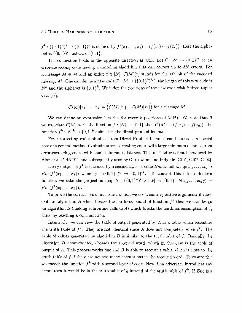
f k : ( (0 , l ) n ) k + ( (0 , l ) ) k is defined by f k ( x l , . . . , xk ) = ( f ( x l ) . . . f ( x k ) ) . Here the alpha-

bet is ((0, I ) ) ~ instead of ( 0 , l ) .

The connection holds in the opposite direction as well. Let C : M + (0, l ) N be an

error-correcting code having a decoding algorithm that can correct up to 6N errors. For

a message M E M and an index x E [ N ] , C ( M ) [ X I stands for the xth bit of the encoded

message M . One can define a new code C1 : M -+ ( (0 , l ) k ) N k , the length of this new code is

N~ and the alphabet is (0, ilk. We index the positions of the new code with k-sized tuples

over [ N ] .

C1(M)[x l , . . . , xk] = ( c ( M ) [ x I ] . . . C ( M ) [ X ~ ] ) for a message M

We can define an expression like this for every k positions of C ( M ) . We note that if

we associate C ( M ) with the function f : [ N ] + ( 0 , l ) then C1(M) is ( f ( X I ) . . . f ( x k ) ) , the

function f k : [ N ] ~ + (0, l)lc defined in the direct product lemma.

Error-correcting codes obtained from Direct Product Lemmas can be seen as a special

case of a general method to obtain error- correcting codes with large minimum distance from

error-correcting codes with small minimum distance. This method was first introduced by

Alon et a1 [ABN+92] and subsequently used by Guruswami and Indyk in [GIOl, GI02, GI031.

Every output of f is encoded by a second layer of code Enc as follows :g (x l , . . . , x k ) =

Enc(f ' ( X I , . . . , x k ) ) where g : ( ( 0 , l ) n ) k + (0, 1ICk. TO convert this into a Boolean

function we take the projection map h : ( (0 , l ) n ) k x [ck] + (0, I ) , h ( x l , . . . , xk, j ) =

E n c ( f k ( x l , . . . , xk)) j .

To prove the correctness of our construction we use a contra-positive argument: if there

exits an algorithm A which breaks the hardness bound of function f k then we can design

an algorithm B (making subroutine calls to A ) which breaks the hardness assumption of f ,

there by reaching a contradiction.

Intuitively, we can view the table of output generated by A as a table which resembles

the truth table of f k . They are not identical since A does not completely solve f k . The

table of values generated by algorithm B is similar to the truth table of f . Basically the

algorithm B approximately decodes the received word, which in this case is the table of

output of A. This process works fine and B is able to recover a table which is close to the

truth table of f if there are not too many corruptions in the received word. To ensure this

we encode the function f with a second layer of code. Now if an adversary introduces any

errors then it would be in the truth table of g instead of the truth table of f k . If Enc is a

good error-correcting code then its decoding algorithm will be able to correct many errors

and obtain a table which will be very close the original truth table of f k . Now if we apply

the algorithm B it will work fine. In essence, the second layer of encoding for the purpose

of preserving the values of the second table .

Chapter 4

Hardness Amplification in small

space

Hardness Amplification in N L with respect to L : We start with a Boolean function

f : (0, l I n -+ ( 0 , l ) which is computable in N L and is mildly hard with respect to algorithms

in L. We want to find a Boolean function h which will be harder than f with respect to

algorithms in L. Ideally we would want f to be & hard and h to be 1 - r hard.

To this end we use the tool called Direct Product followed by an encoding by a 'good'

binary error-correcting code. As we discussed in the previous chapter the direct product

function f k : ((0, l)n)k + {O, l)IC is defined as (f (xl) , . . . , f (xk)). In our constructions we

will prove h(xl, . . . , x k ; j ) = ~ n c ( f ~ ( x 1 , . . . , x ~ ) ) ~ is O(1)-hard against logspace algorithms.

The correctness of the construction is proved by a contra positive argument. We start by

assuming there exists an algorithm A working within L which computes h on more than a

constant fraction of inputs. Using that we design another algorithm B in L which computes

f on more than 1 - l/poly(n) fraction of inputs thereby arriving a t a contradiction. To

design the algorithm B we need to be able to decode the concatenated codes inside out.

That is, we first decode the binary error-correcting code followed by the direct product code.

We need some kind of a "voting scheme" by which we can predict the value of f on every

input. Note that the direct product function is viewed as an error-correcting code in the

manner we discussed in the previous chapter. The voting scheme requires us to generate

k-tuples from a smaller string in a space efficient manner. Writing down the entire tuple

explicitly on the tape would require nk tape cells. We need a space efficient deterministic

function G which takes a seed of size n+O(log n) and generates k, n length strings implicitly.

The input string is of size n and we are allowed an additional O(1og n) bits. We expect the

tuple generated by G to have some dependence. However we do hope that f k ( ~ ) will have

approximately the same average case hardness as f k on completely independent xi's.

Apart from N L we also look at the problem of hardness amplification in NLINSPACE.

Here the starting function f can be worst case hard against algorithms in LINSPACE.

4.1 Limitat ions

If a problem is hard then several independent instances of the problem should be propor-

tionately harder. An algorithm trying to compute a hard function on several inputs is likely

to make many more mistakes than it would on a single input.

The problems we are addressing in this thesis, namely hardness amplification in non-

deterministic linear space and nondeterministic logspace require a pseudorandom generator

since we cannot afford to use kn space for any non constant k. For NL we only have log-

arithmic space on the work tape and for N L I N S P A C E there is an additional O(n) space

on the tape. So for a non constant k, the use of a pseudorandom generator is imperative.

Ideally we would like to prove that there is a way to pick k pseudo random instances of

a hard problem/function using fewer than kn random bits and the direct product of f (xi)s

is still just as hard to compute as if the instances were independent. The standard N W

generator and simple use of expander walks do not give the desired result.

When the computation is time bounded as opposed to space bounded , we have more

flexibility to use space. Clearly the amount of used space cannot exceed the total computa-

tion time, for instance in N P one has at disposal polynomial amount of space. The generator

can now use polynomial length seed to generate the instances. However for space bounded

classes especially in sub-linear classes like N L the generator seed plays a crucial role. The

value of k depends on the hardness we are trying to achieve. If we want the final hardness to

be around 1/2+ (1 - 26)k then this is approximately equal to 1/2+ l/poly(n) if k = O(1og n).

The one advantage that nondeterministic space bounded classes have over time bounded ones

are the property of closure under complementation, NSPACE(s(n)) = coNSPACE(s(n)).

This property ensures that the new function remains within the old class.

The known generators like the one suggested by Imapgliazzo and Wigderson in [IW97]

, which is a combination of two previously known generators, namely Nisan-Wigderson

generator and expander walk generator do not meet our requirements. A crucial aspect

of their construction is the use of "designs". The problem with this construction is that

for those parameters which are of interest to us there are no designs! Hence one needs to

construct a generator possibly from scratch which meets our criterion.

4.2 Our Result

In the next two chapters we will discuss our constructions in details. We are able to show

for both N L and N L I N S P A C E amplification up to a constant fraction. We use two tech-

niques one due to Trevisan as suggested in [Re031 and the other one due to Guruswami

and Kabanets as in [GK06]. Both the techniques are derandomized expander based direct

product construction and they yield the same result. Trevisan construction looks at neigh-

borhood of a vertex and applies the function on the vertex labels of the neighborhood set

where as the other technique applies the function to every vertex appearing on expander

walks starting at a given vertex and specified by edge labels. For LINSPACE we are able

to go from worst case to average case hardness without using a derandomized direct product

construction. We simply apply a suitably chosen error-correcting code and that alone gives

the required amplification result.

Chapter 5

Construct ions in Nondeterministic

Logarithmic Space

In this chapter we discuss ways to construct a function with constant hardness starting from

a function with inverse polynomial hardness.

We use two different construction techniques and compare the parameters achieved by

each. The first technique is as suggested by Trevisan in [TreOS] and the second one follows

in the line of [GK06].

The general scheme is:

1. Define an expander based direct product using the input function.

2. Encode each output of the direct product function with a suitable binary error-

correcting code.

3. Transform to a Boolean function by concatenating all binary strings output by the

function in step (2) .

We start off by introducing notations we will be using in this chapter. The ith neighbor

of a vertex x in some graph G is denoted by Ni(x ) , the underlying graph G will be clear

from the context. The degree of the graph is denoted by d. For ease of notation we may

use N ( x ; i ) instead of Ni(x ) . If x is the j th neighbor of some vertex y then we will use

N ( x ; i ) = (y; j) to denote that. Since we will be dealing with undirected graphs or

bidirectional graphs at all times, adjacency relation is symmetric. The kth bit of string

x is denoted by xk. A t length path starting at x and indexed by ( i l , . . . , i t ) is denoted

by (x; i l , i2, . . . , i t ) . In other words the walk can be described as (x, x l , x2,. . . , xt) where

xl = N(x, i l ) , x2 = N(x l ; i2) = N(N(x ; i l ) ; i2) and so on. The constructions use some

error-correcting code whose encoding function will be commonly denoted by Enc.

5.1 Construction Techniques

The direct products for a function f in the constructions can be described in two ways. One

which uses the neighborhood of a given vertex and the other which uses a expander walk

starting from a vertex.

The first one evaluates f on all the neighbors of a given vertex to define the first direct

product. We will be referring to this as Neighborhood construction (I) or Trevisan's con-

struction. The second one deals with expander walks indexed by the edge labels (21, . . . , i t )

and will be referred to as Walk construction (11) or Guruswami-Kabanets technique.

One important aspect that is common to both the techniques and both the classes is

that the resulting function h belongs to the same class as the initial function f .

A Boolean function f is in a complexity class C if and only if the associated language

Lf = { X I f (x ) = 1) is also in C. To say a Turing machine computes a non-Boolean

function g : {0,1)* + (0, I)* in nondeterministic O(s(n)) space means that there exists a

nondeterministic Turing machine using O(s(n)) space which on every input (xl , . . . , xt) has

at least one accepting computation. The work tape a t the end of each accepting computation

contains the exact same string which is the value of g on that input.

5.2 Mixers

In the constructions to follow, we will first show amplification using Trevisan's technique

followed by the one suggested by Guruswami and Kabanets. For each we will discuss the

proof of correctness of the respective algorithms and how the bounds can be achieved within

the allowable space.

The crucial aspect of the (I) construction is the use of mixers.

Definition 12 A d-regular bipartite graph G = (L, R, E) where ILI = IRJ = N, N = 2n is

an (E, 6) mixer if for every subset B C R of vertices such that IBI 5 ( a - E)N there are at

most 6N vertices v in L such that Ir(v) n BI > 2 where r (v ) is the set of neighbors of v.

For constructions in N L we need an implicit representation of the neighborhood, that

is the algorithm computing the neighborhood will take as input a vertex v and two indices

i , j and output N ~ ( v ) ~ the jth bit of the ith neighbor of v.

One way to increase the connectivity of the graph G is by powering. The graph G~

is the ith power of G if all vertices connected by walks of length i in G are neighbors in

G ~ . The adjacency matrix of G~ is the i th power of the adjacency matrix of G. If A is

the adjacency matrix of G then Ai is the adjacency matrix of Gi. Analogously, if X is the

spectral expansion of G then Xi is the spectral expansion of Gi.

For each eigenvalue of the normalized adjacency matrix, its absolute value is an eigen-

value of the graph. The normalized adjacency matrix is symmetric and so by results in

Linear Algebra the eigenvalues are all real.

The eigenvalue gap is the difference between the first and second value. Regular Bipartite

graphs have eigenvalue 1 with multiplicity 2, as both d and -d are eigenvalues of the

adjacency matrix. As a result the eigenvalue gap of a regular bipartite matrix is 0.

For the neighborhood construction we need mixers whose eigenvalue gap satisfies a cer-

tain relation. By definition a mixer is a regular bipartite graph and so the eigenvalue gap

should be 0. To fix this problem we can convert the graph to a non-Bipartite graph without

changing the graph too much. For every vertex in Vl we can associate a vertex on the

right and to make it a regular graph we can add self loops. This new graph will retain the

property essential for our proofs to work and yet produce a non-zero eigenvalue gap.

For the parameters of our interest we will have to prove a result of the following kind.

Lemma 2 There are (E, 6)-mixers with degree d = poly(:, i)

Proof: The vertex set of a Gabber-Gallil graph is (Z2n x Zp, Z p x Z p ) . We will prove that

a constant degree modified Gabber-Galil graph on 2~~ vertices is a mixer if its eigenvalue

gap satisfies a certain relation.

A degree d bipartite graph does not have an eigen value gap since its first two eigen values

is ]dl. To convert the Gabber-Galil graph into a non bipartite graph we asociate each vertex

in Vl to a vertex in V2. Since originally it was a degree 5 graph the new graph has degree

at most 8. One can add self loops to each vertex to make this a degree d graph for some

d > 5. This new graph will retain the constant vertex expansion property of the original

graph , since the neighborhood of each vertex has (possibly) expanded by a constant. Using

theorem 3 we conclude that constant vertex expansion implies constant spectral expansion.

The mixing property of expander graphs gives us the following:

We want to construct a (E, 6)-mixer for a given E and 6. We take T G V2 such that

IT1 5 (112 - e)N2 as defined in the definition of mixers and S to be {v E & I IN(v) f l TI > d/2) G Vl implying that e(S, T ) > q. We obtain this following relation,

If ($$$)2(1 -2') <- 6 then we obtain IS1 5 6N2 as required by the definition of mixers.

On simplifying the above relation we get

We start with a degree 5 Gabber-Glil graph, convert it into a constant degree non-

bipartite graph and then power it to a suitable exponent so that the spectral expansion of

5.3 CONSTRUCTIONS I N NONDETERMINISTIC O(10g n) SPACE 24

that graph will satisfy the above condition. Now we convert this graph back to a bipartite

graph by creating an identical copy of the vertex set and for every edge between a pair of

vertices vl and v2 in the non-bipartite graph we replace with an edge between vl and v2 in

the left and right bipartition respectively.

The bipartite graph so formed will be the required ( E , 6 ) mixer.

0

In what follows, we will discuss in two separate sections hardness amplification in N L .

We will discuss in details the neighborhood construction as well as the walk construction.

The first one requires implicitly constructible mixers but the walk construction can be

applied to any constant degree expander.

5.3 Constructions in nondeterministic O(1og n) space

5.3.1 Trevisan's construction

Theorem 7 Given a Boolean function f E N L , such that f is & hard (r is constant) with

respect to L , we can obtain a Boolean function h E N L such that h is O(1) hard with respect

to L using the direct product construction described in [Tre03].

Proof: We will define a non-Boolean function g from which we will obtain the Boolean

function h which meets the hardness requirement.

The direct product is defined by f d : (0 , l In -+ (0 , l ) d , f d ( x ) = f ( N l ( x ) ) . . . f ( N d ( x ) ) .

The concatenated code is defined by g : (0 , l Id -+ (0 , g (x ) = ~ n c ( f ~ ( x ) ) . To convert

to a Boolean function we take a projection map h : (0, l jd x [cd] -+ {0 ,1) which is defined

as h ( x , i ) = g(x) , , 1 5 i _< cd where Enc is an error correcting code.

We will first show that f d is a - E hard for a small consant E . The application of the

error-correcting code will reduce the hardness by a constant factor.

2. Existence of ( E , l / n r ) mixers on ( [ N ] , [ N ] ) vertex set for E = 0.1 .

In the constructions to follow the parameters 6 and 61 are respectively the hardness of

the initial function and the hardness of the encoded Direct product function. Therefore

we want 6 = l / n r for a constant r and = 112 - E and that makes the degree of the

mixer to be poly(n).

3. Decoding algorithm uses a voting scheme, we need to show that it works.

The proof of correctness of decoding algorithm will prove this.

Claim 1 There exists a ( E , l /nT) mixer which is implicitly constructible in O(1ogn) space.

Proof: We will argue that we can use Gabber Galil graphs to construct (r, l /nT) mixers

of degree poly(n). Instead of computing the polynomial degree graph ( call it G2) from the

constant degree G1, we will compute the neighborhood function of G2 implicitly.

To obtain G2 from GI we need to walk on GI for O(1ogn) steps. Edge labels in GI

need O(1) bits and by using the logarithmic space algorithm due to Chiu-Litow-Davida,

Fortnow-Klivans and Gutfreud-Viola (Theorem 5) we can find the final vertex on such

paths in O(1ogn) space. This algorithm finds the vertices implicitly and so we compute

the neighborhood relation of G2 implicitly. That is, given (x, i , j ) where x E (0, l In and

i E [dl, j E [n] we can find the j th bit of the ith neighbor of x . Lemma 2 says we can

construct the required mixer if we use the powering operation on a Gabber-Galil graph such

that the resulting graph's spectral expansion satisfies a relation.

For our construction we would need a set S to be of size at most $$ and T to be of size

at most (4 - t ) ~ ' . The graph would then satisfy the relation

This simplifies to X < & (1 + 2r)(l + r) if 6 = &.

The above claim proves that we can implicitly construct (6, l/poly(n))-mixers on ([N], [N])

vertex set where E is a constant. We will use that graph for our construction.

Lemma 3 If h is as defined before then it is computable in nondeterministic logspace.

Proof: We will argue that g is computable by a nondeterministic Turing machine and since

h is just a projection map of g it must be true that h is also computable by a nondeterministic

machine.

Define Lf = { X I f (x ) = 11, NL = coNL implies if Lf is in NL then coLf is also in NL.

Then there must exist two nondeterministic logspace machines Ml and Mz computing Lf

and coL respectively.

We design a machine M which computes g as follows:

Input : x

Output: g(x) = ~ n c (f (xl) . . . f (xd)) where Ni(x) = xi for each 1 5 i 5 d.

For each i from 1 to d,

Step 1: Nondeterministically guess computations for MI and M2.

Step 2: Simulate the computations of M1 and M2 and set the value of bi as follows,

1. If M1 accepts then set bi = 1.

2. If M2 accepts then bi = 0.

3. Else if both M1 and M2 end in rejection then set bi = 0 and reject.

Step 3: Collect all the answers bi for each xi, 1 5 i 5 d. Run the error-correcting code

Enc on (bl bk) and output the answer and end in accepting state.

Clearly this is a nondeterministic machine. For every input (xl, . . . , xk) the machine ends

in a t least one accepting run. And every time that happens the value on the work tape is

Enc(f (21) . . . f ( ~ d ) ) .

We need to argue that g can be encoded in logspace. Since g(x) is of polynomial length

we will need to represent it implicitly. That is on input (x, i ) the algorithm must generate

the i th bit of g(x), which is nothing but h(x, i ) . So if g is in N L then so must be h.

The logspace constructibility of g follows from our choice of error-correcting code which

is logspace encodable and decodable (Spielman code, theorem 6) and the availability of a

logspace neighborhood finding algorithm. We generate fd(x) bit-by-bit. The input bits

to the encoding function Enc is generated on the fly, say if it requires kth bit of the i th

neighbor then we find f (Ni(x))k by reusing all the space that was used before. At any given

time we do not store anything, we simply compute it from scratch.

Therefore g is in N L and as discussed before that implies h is in N L too. 0

To argue the correctness of the construction we will first show that if there exists an

algorithm Afd such that Afd solves f d on more than 112 + E fraction of inputs in space

O(1og n) then there exists an algorithm Af which solves f on more than 1 - l / n r fraction

of inputs in O(1ogn) space. We finish by proving that h must be of constant hardness. We

start with the following.

Claim 2 f d is (+ - E) hard against logspace algorithms given that f is & hard in L.

Proof: Assume f d can be computed on more than 112 + E fraction of inputs by a logspace

algorithm A j d . In order to reach a contradiction we will design an algorithm Aj which will

be break the hardness assumption of f .

On input x : Do the following.

For i going from 1 to d:

1. Compute Ni(x).

2. Find bi = A jd (Ni ( x ) ) ~ where f (x) is in the kth position of f d ( ~ i ( x ) ) .

Writing down the whole string Ni(x) is not possible since we are only allowed O(1og n)

space. We use the logspace algorithm by Fortnow, Klivans and Chiu , Litow, Davida

which gives the implicit representation of such a vertex. In other words we generate

Ni(x) bit by bit as and when the algorithm Ajd requires it.

3. Output Majorityi{bi} as the predicted value of f (x).

To be able to do majority vote in O(1ogn) space we keep track of three values: i,

number of 0s seen so far and number of 1s seen so far. Since i 5 poly(n) these values

can be represented and updated in O(1ogn) space. At the end of all the votes we have

the number of 0s and Is. Which ever is more is the predicted value of f (x).

The correctness of the algorithm A j d follows from the mixer property of the graph. Let

the set of strings on which A j d makes a mistake be defined as

Bad = {x I A j d (x) # f d(x)).

By assumption Ajd solves f d on more than 112 + E fraction of inputs so

and similarly we define

For any x to be in B a d f , A f d must be wrong on majority of neighbors of x . That is at

least ( d l 2 + 1) neighbors of x are in B a d f d .

Using the definition of mixer we conclude that lBadf 1 5 $. Therefore the fraction of inputs on which As is correct is at least ( 1 - l /nT) . This is a

contradiction to the assumption that f is l /nT hard and so we conclude that f d must be

(112 - E ) hard.

0

Claim 3 If h is as defined before, then it is dlp/2-hard with respect to L given that f d is

&-hard with respect to logspace algorithms where p is the constant relative distance of the

error- correcting code.

Proof: Assume there exist an O(1ogn) space algorithm Ah which computes h . We can

design an algorithm A which can compute f d implicitly.

On input x , do the following:

R u n the decoding algorithm Dec o n A h ( x , j ) bit by bit where j goes from 1 to cd.

This can only be an implicit algorithm since we cannot write down the whole string f d ( x )

on the work-tape as it will take O ( d ) = poly(n) bits. This is clearly a logspace algorithm if

E n c - Dec is chosen to be a logspace encodable-decodable code and Ah works in O(1ogn)

space.

Define Badh to be

{ ( x i i ) lh(xi i ) # A h ( ~ 7 2 ) )

and

For each x E Bad the string

is at least $ relative Hamming distance away from the actual ~ n c ( f ~ ( x ) ) .

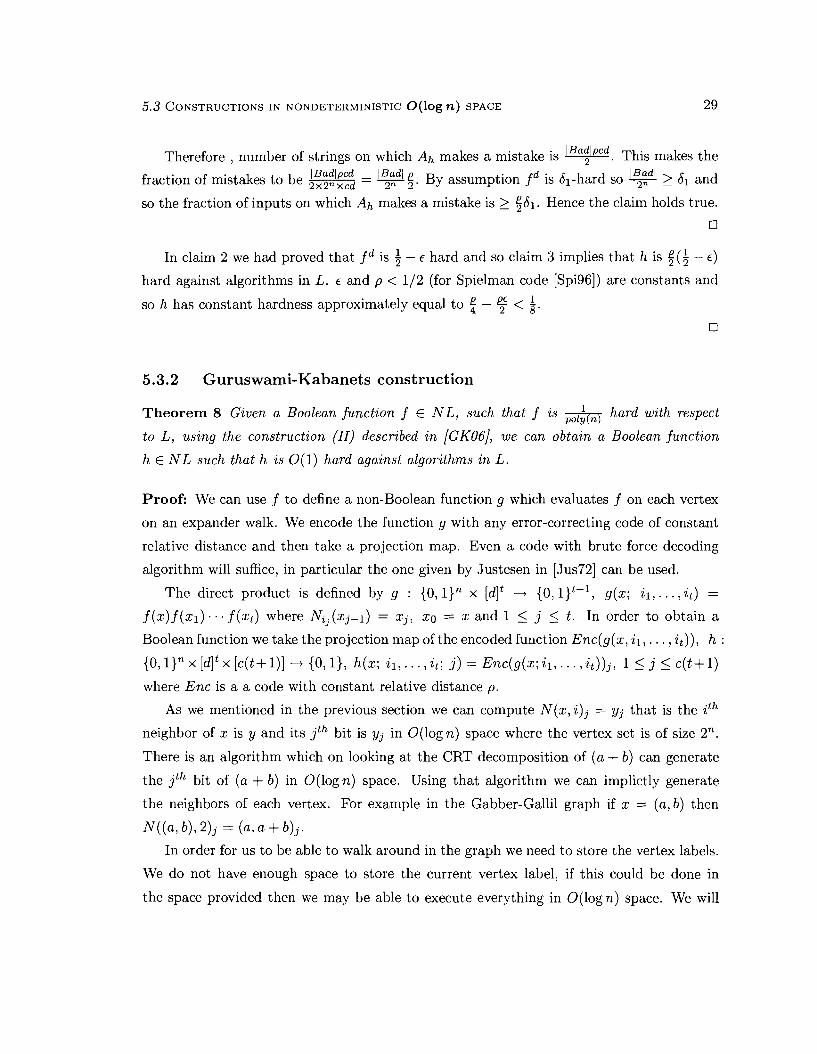
Therefore , number of strings on which Ah makes a mistake is v. This makes the

fraction of mistakes to be = q:. By assumption f d is 61-hard SO > 61 and

so the fraction of inputs on which Ah makes a mistake is > $dl. Hence the claim holds true.

0

In claim 2 we had proved that f d is 4 - E hard and so claim 3 implies that h is $(a - E)

hard against algorithms in L. E and p < 112 (for Spielman code [Spi96]) are constants and

so h has constant hardness approximately equal to 2 - 5 < i. 0

5.3.2 Guruswami-Kabanets construction

Theorem 8 Given a Boolean function f E NL, such that f is & hard with respect

to L, using the construction (11) described in [GK06], we can obtain a Boolean function

h E N L such that h is O(1) hard against algorithms in L.

Proof: We can use f to define a non-Boolean function g which evaluates f on each vertex

on an expander walk. We encode the function g with any error-correcting code of constant

relative distance and then take a projection map. Even a code with brute force decoding

algorithm will suffice, in particular the one given by Justesen in [Jus72] can be used.

The direct product is defined by g : (0, lIn x [dlt -+ {O,l)t+l, g(x; i l , . . . , i t ) =

f (x) f ( x l ) . . . f (xt) where Nij(xj-1) = xj, xo = x and 1 5 j 5 t. In order to obtain a

Boolean function we take the projection map of the encoded function Enc(g(x, il, . . . , i t)) , h :

{0,1)" x [dlt x [c(t+ 1)] --t (0, I) , h(x; il, . . . , it; j ) = Enc(g(x; il, . . . , i t ) ) j , 1 I j 5 c(t+ 1)

where Enc is a a code with constant relative distance p.

As we mentioned in the previous section we can compute N(x, i)j = yj that is the ith

neighbor of x is y and its jth bit is yj in O(1ogn) space where the vertex set is of size 2n.

There is an algorithm which on looking at the CRT decomposition of (a + b) can generate

the jth bit of (a + b) in O(1ogn) space. Using that algorithm we can implictly generate

the neighbors of each vertex. For example in the Gabber-Gallil graph if x = (a, b) then

N((a , b), 2)j = (a, a + b)j.

In order for us to be able to walk around in the graph we need to store the vertex labels.

We do not have enough space to store the current vertex label, if this could be done in

the space provided then we may be able to execute everything in O(1ogn) space. We will

compress the vertex labels by storing the value modulo a sufficiently big prime such that

the vertex can be now be represented in O(1ogn) space.

Since x is given as the input, we can calculate f (x) in O(1ogn) space. We can not

write down X I , the next vertex on the walk, explicitly on the tape. The Turing machine

only requires to know one bit at a time so we generate the required bit using the implicit

representation of XI. The relation N(x, i l ) k for each k does that. This works for xl since

x is present in the input tape and to generate each bit of xl which is a neighbor of x the

tape head can look up x on the input tape. But to calculate xt even bit by bit , we need

the explicit representations of X I , 2 2 , . . . , xt-1. That is why we store xi mod p for each i

between 1 and t . The prime p is chosen such that it can be represented in O(1ogn) bits

and so xi mod p does not require more than logarithmic space. As and when we require

a particular bit of xi we invoke the logspace Chinese Remainder representation to implicit

binary representation algorithm (Theorem 2) and after we are done we restore xi mod p.

To prove the theorem we need to argue the following things:

1. h E NL.

2. Proof of correctness of the construction , that is h is indeed constant hard with respect

to L.

Lemma 4 If f is nondeterministic logspace computable then h is also nondeterministic

logspace computable.

Proof: To prove that g is in N L we follow the same argument as the one we gave for

Trevisan's construction. The only difference here is the definition of xis. There they were

neighbors of x and here they are vertices on a walk passing through x. Other than this all

other details remain the same.

0

In order to prove the correctness of the construction one needs to show that if there

exist a logspace algorithm Ag which can solve g on more than 1 - 26 fraction then we can

design an algorithm in L which can solve f on more than 1 - 6 fraction of inputs. The above

discussion about logspace computable walks ensure that all the necessary computations can

be carried on in logspace.

We will give an informal description of the decoding algorithm and then follow it up by

a formal algorithm.

Claim 4 Suppose f is 6-hard for logspace. Let t 5 then the function g defined above is

R(tb) -hard for logspace.

Proof: Assume there exists an algorithm Ag which solves g on more than 1 - b' fraction of

inputs for the least possible value of 6'. One can use Ag to design an algorithm to compute

f . Informal Idea : On input x E (0, l jn for each i E (0, . . . , t), we record the predicted

majority value bi for all possible t step walks which pass through x in the i th step. Using

our above notations that would mean the majority taken over all values (Ag(w))i where w

is a t-step walk in the graph G that passes through x in the ith step and (Ag(w))i is the

ith bit in the (t + 1)-tuple output by the algorithm Ag on walk w. Now we take another

majority vote over all bis ( 1 5 i < t). This value is the predicted value of f (x). What this

does is place x in each position of all possible t length walks in the graph and keep count

of the predicted value of f on them. Then we take a double majority vote and that is the

predicted value of f on the input x. See below for a presentation of this algorithm.

Each element of the tuple (kl, . . . , kt) indexing a walk can be generated one by one in

O(1ogn) space and then the space can be reused for the next element. This is a constant

degree expander and so to store each label we only require O(1) bits. By assumption Ag(w)i

takes logarithmic space, so everything can be done in O(1ogn) space.

On input x E (0, l jn

GOAL : To compute f (x)

2. for each i = 0 to t

4. for each t-tuple (kl, kg, . . . , kt) E [dlt

5. Compute the vertex y reached from x in i steps by taking edge labeled kl, . . . , ki.

7. end for

8. if c2 2 dt/2 then cz = cl + 1

9. end if

10. end for

11. if cl 2 t / 2 then RETURN 1 or else RETURN 0.

Proof of correctness of A f follows in the same line as the proof presented in [GK06]. We

will skip the detailed calculations. The conclusion is that 6' 2 R( t ) Pr,[Af ( x ) # f ( x ) ] 2

R(t)6. 0

Lemma 5 Suppose g is &-hard against logspace algorithms. Then the function h is h1p/2

hard for algorithms in L were p is the constant relative distance of Enc.

Proof: Let us assume Ah computes h on more than 1 - 6' fraction of inputs for the least

possible 6' achievable by algorithms in L.

Algorithm Ag follows : On input ( x ; i l , . . . , i t ; j ) compute Ah(x; i l , . . . ,it; j ) for all

j E [c(t + l ) ] where as always l / c is the rate of Enc. Apply Dec to the obtained string

and output the decoded string. Since t and c are constants we can do this computation in

logspace.

Now we will analyze the fraction of inputs on which Ah makes mistake. Let us con-

sider the set Bad = { ( x ; i l , . . . , i t ) lAg((x; i l , . . . , i t ) ) # g( (x ; i l , . . . , i t ) ) ) , basically the

set of inputs on which Ag makes a mistake. For each ( x ; i l , . . . ,it) E Bad , the string

[Ah(x; 21,. . . , i t ) l , . . . , Ah(x; i l , . . . , it)c(t+l)] is at least p/2 relative Hamming distance away

from the actual encoding Enc(g(x; i l , . . . , i t ) ) . Number of inputs on which Ah makes a

mistake is at least JBadl$c(t + 1). This means the fraction of inputs on which Ah makes

mistakes is where 2" x dt x c(t + 1) is the total number of possible inputs

to Ah. After canceling out common terms from the numerator and denominator we get I Bad1 P

2 x 2 " x d '

If g is 61 hard then 2 61 therefore fraction of inputs on which Ah makes mistakes

is 2 gw = 9. We took Enc to be a constant distance code so 9 = R(61).

0

Note that we have obtained amplification from 6 to t6p/2 as 61 = R(t6). If we apply

this construction repeatedly, the hardness increases constant time with every iteration. At

the end of s steps we go from 6 to (!f)'6. Since t and p are constants we can choose s to be

log? = O(1og f ) in order to obtain the final constant hardness.

We conclude that the construction does meet the hardness bound, or in other words we

can amplify from inverse polynomial to constant hardness against logspace algorithms.

0

One aspect where Trevisan's construction scores over the other is the input length.

Input length of the starting function is n bits. After applying the Guruswami-Kabanets

construction we obtain a function whose input size is n + t log d+log(c(t+ 1)) = n+O(t log i) bits. In Trevisan's construction the input length of the final function is n + log c(t + 1) bits.

The following table gives a comparison between the two constructions.

Table 5.1: The two methods a t a glance Neighborhood Construction Walk Construction

Size of input n n + k [log dl

Size of Direct Product P O ~ Y ( ~ ) o(l> Amplification 6 + 0 ( 1 ) 6 -+ 26

Chapter 6

Construction in Nondeterministic

Linear space

Given a function f of hardness & we want to generate a function h which is of constant

hardness.

This amplification does not require a Direct product construction. We will encode the

function with a suitable error-correcting code and then take the projection map to obtain

the Boolean function.

Theorem 9 Given a Boolean function f : (0, l j n + {0,1), f E NLINSPACE, such

that f is A- hard with respect to LINSPACE, we can obtain a Boolean function h E

NLINSPACE such that h is O(1) hard with respect to LINSPACE.

Proof: We concatenate it with an logspace encodable/decodable error-correcting code Enc

like in [Spi96]. Enc : (0, 1j2" + (0, 1jC2" where l / c is the constant rate and p is the

constant relative distance of the code. We define a string X which is the encoding of the

truth table of f , i.e, X = Enc(TT( f ) ) . In order to convert this into a Boolean function we

take the projection map h : [ ~ 2 ~ ] + (0, I), h ( j ) = E ~ c ( T T ( ~ ) ) ~ .

Claim 5 If h is as defined before then it is computable in nondeterministic O(n) space.

Proof: The truth table of f can be viewed as a message of size 2n. The encoding of this

message will be a string of size ~2~ for a constant c. The error-correcting code is logspace

encodable and decodable, so we only require O(n) space to implicitly compute X.

CHAPTER 6. CONSTRUCTION IN NONDETERMINISTIC LINEAR SPACE 3 5

Since N L I N S P A C E = c o N L I N S P A C E and f E N L I N S P A C E we can use the same

argument as we did in our previous constructions to conclude that g is in N L I N S P A C E

and consequently h is a Boolean function which is computable by nondeterministic linear

space algorithms.

0

Claim 6 Let h and f are as defined before. Given f be &-hard then h must be y-hard

where y is the fraction of errors corrected by the error-correcting code.

Proof: A linear space algorithm Ah computes h correctly on some fraction of inputs. We

will use this to design an algorithm which computes f .

On each input x do the following :

1. Find A h ( i ) for every 1 5 i < ~2~ and run the decoding algorithm Dec on the implicitly

generated string A h ( l ) A h ( 2 ) . . . A h ( d n ) .

2. Output the bit which corresponds to the value of f (x), we denote that by

Dec[Ah( l ) . . . A h ( ~ 2 ~ ) ] ~ .

Since f is worst case hard , there exists at least one string x for which Dec[Ah( l ) . . . Ah ( ~ 2 ~ ) ] ~

is different from f ( x ) . The fraction of errors that the Dec algorithm can correct, i.e the

fraction of positions in the string A h ( l ) . . . A h ( d n ) which are different from h(1) . . . h ( ~ 2 ~ )

is at most y. Let us define the set Badh as {il Ah( i ) # h ( i ) ) , so if lBadhl < 7 ~ 2 ~ then the

value of D e c [ A h ( l ) . . . A h ( ~ 2 ~ ) ] at position x is correct. Therefore h must be y hard.

0

If we use an error-correcting code which corrects a constant fraction of errors like the

Spielman code [Spi96] then h is O ( 1 ) hard and as discussed in a previous chapter for binary

codes error correction can be at most up to a quarter fraction.

0

Chapter 7

Conclusion

In order to push the hardness beyond the 114 fraction in both N L and NLINSPACE, we

need to devise new derandomized direct product results. Derandomization is crucial, since

due to the lack of space we cannot write k instances of n length string on the tape. We would

like to have a generator G which will take a small seed to generate a tuple (xl, . . . , xk) , on

which we will define the new direct product construction.

The length of x cannot exceed n + log n.

There are a few derandomized direct product lemmas. The one used in [IW97] is a

combination of two generators, expander walk generator EV(v, 2) and Nisan-Wigderson

generator NW. They combine the two generators together to form a new XOR generator

XG(r; r'; v; d) as follows: Use r to select a (yn, n)-design where the universe is the set

(1, . . . , d). Then N W (x) = (xIsl, . . . , XIS,) and E W(V, 2) = (vl, vz, . . . , vk). The resulting

generator XG[r;r1; v, d] = (xlsl @ vl, xlsz @ va, . . . , xlsk @ v,). In order to use this we need

C = {S1, . . . , Sk), a family of subsets of [dl of size n. For every i # j , JSi nSj I 5 yn for some

constant y. Let r E (0, l Id and S = {sl, . . . , s,) C [dl. Then let the restriction of r to S, rls

be the n-bit string rls = r,,r,, . . .r,,,. Then for a y-disjoint C, ND' : (0, lIrn --t ((0, l )n )k

is defined by: N D' ( r ) = r Is, . . . r 1 sk. The parameters of interest to us are d = n + log n

but then the condition ISi nSj( 5 yn for a constant y is impossible. As after the first set S1

has been selected, the number of unpicked elements is logn and hence any subsequent set

Si will have at least n - logn intersections with previously picked sets. So a random walk

on graphs in conjunction with combinatorial designs will not yield the desired generator.

CHAPTER 7. CONCLUSION 37

The first encoding step of the direct product needs to be followed by another layer of

encoding by a suitably chosen error-correcting code. Since we are trying to push hardness

past quarter fraction the error correcting code needs to be list decodable. This is because

unique decoding for binary codes beyond quarter fraction is not possible. Any list decodable

code will not suffice, it needs to be a locally decodable code. While working in logarithmic

sized space, writing down entire codeword or message is not possible, yet we want to generate

the list of messages which may have generated a particular codeword. To facilitate this we

allow implicit representation of codewords and messages. Locally decodable codes allow us

to do this. As an input the decoding algorithm takes a codeword and an index i and outputs

a list of algorithms one of which finds the ith symbol of the message which gave rise to the

codeword.

The error-correcting code suggested by Sudan, Trevisan and Vadhan in [STV99] is a

multivariate polynomial based code. Part of the construction requires finding polynomials

of degree d in the field F . Such polynomials can be indexed by d log IF[ bits. The size of F is

roughly equal to O(n2). Due to the restriction in space we cannot write down a polynomial

which is super linear in n. As a result we cannot use this code.

Our future course of action is to find a derandomized direct product result for seed

length n + O(1og n). In particular we would like to know if the two expander based direct

products we have used in our constructions may be sufficient to amplify hardness beyond a

quarter fraction. Even without the restriction on space can we find a derandomized direct

product which pushes the hardness beyond ?

Bibliography

[ABNf92] N. Alon, J. Bruck, J. Naor, M. Naor, and R. Roth. Construction of asymptotically good low-rate error-correcting codes through pseudo-random graphs. IEEE Transactions on Information Theory, 38:509-516, 1992.

[A10861 Noga Alon. Eigenvalues and expanders. Combinatorica, 6:86-96, 1986.

[BFNW93] L. Babai, L. Fortnow, N. Nisan, and A. Wigderson. B P P has subexponen- tial time simulations unless EXPTIME has publishable proofs. Computational Complexity, 3:307-318, 1993.

M. Blum and S. Micali. How to generate cryptographically strong sequences of pseudo-random bits. SIAM Journal on Computing, 13:850-864, 1984.

A. Chiu, G. Davida, and B. Litow. Division in logspace-uniform NC'. RAIRO - Theoretical Informatics and Applications, 35(3):259-275, 2001.

L. Fortnow and Adam R. Klivans. Linear advice for randomized logarithmic space. In Proceedings of the Twenty-Third Annual Symposium on Theoretical Aspects of Computer Science, pages 469-476, 2006.

0. Gabber and Z. Galil. Explicit construction of linear sized superconcentrators. Journal of Computer and System Sciences, 22:407-420, 1981.

V. Guruswami and P. Indyk. Expander-based constructions of efficiently decodable codes. In Proceedings of the Forty-Second Annual IEEE Symposium on Foundations of Computer Science, pages 658-667, 2001.

V. Guruswami and P. Indyk. Near-optimal linear-time codes for unique decoding and new list-decodable codes over smaller alphabets. In Proceedings of the Thirty-Fourth Annual ACM Symposium on Theory of Computing, pages 812- 821, 2002.

V. Guruswami and P. Indyk. Linear-time encodable and list decodable codes. In Proceedings of the Thirty-Fiflh Annual ACM Symposium on Theory of Com- puting, pages 126-135, 2003.

BIBLIOGRAPHY 39

V. Guruswami and V. Kabanets. Hardness amplification via space-efficient direct products. In Proceedings of the Seventh Latin American Symposium on Theoretical Informatics, pages 556-568, 2006.

D. Gutfreund and E. Viola. Fooling parity tests with parity gates. In Proceedings of Eighth International Workshop on Randomization and Computation, pages 381-392, 2004.

A. Healy, S. Vadhan, and E. Viola. Using nondeterminism to amplify hardness. In Proceedings of the Thirty-Sixth Annual ACM Symposium on Theory of Computing, pages 192-201, 2004.

N. Immerman. Nondeterministic space is closed under complementation. SIAM Journal on Computing, 17(5):935-938, 1988.

R. Impagliazzo. Hard-core distributions for somewhat hard problems. In Pro- ceedings of the Thirty-Sixth Annual IEEE Symposium on Foundations of Com- puter Science, pages 538-545, 1995.

R. Impagliazzo and A. Wigderson. P=BPP if E requires exponential circuits: Derandomizing the XOR Lemma. In Proceedings of the Twenty-Ninth Annual ACM Symposium on Theory of Computing, pages 220-229, 1997.

R. Impagliazzo and A. Wigderson. Randomness vs time: Derandomization under a uniform assumption. Journal of Computer and System Sciences, 63(4):672-688, 2001. (preliminary version in FOCS'98).

J . Justesen. A class of constructive asymptotically good algebraic codes. IEEE Transactions on Information Theory, 18:652-656, 1972.

N. Nisan and A. Wigderson. Hardness vs. randomness. Journal of Computer and System Sciences, 49:149-167, 1994.

R. O'Donnell. Hardness amplification within NP. Journal of Computer and System Sciences, 69(1):68-94, 2004. (preliminary version in STOC'02).

D.A. Spielman. Linear-time encodable and decodable error-correcting codes. IEEE Transactions on Information Theory, 42(6):1723-1732, 1996.

M. Sudan, L. Trevisan, and S. Vadhan. Pseudorandom generators without the XOR lemma. In Proceedings of the Thirty-First Annual ACM Symposium on Theory of Computing, pages 537-546, 1999.

R. Szelepcse'nyi. The method of forcing for nondeterministic automata. Bulletin of the European Association for Theoretical Computer Science, pages 96-100, 1987.

BIBLIOGRAPHY 40

[Tre03] L. Trevisan. List-decoding using the XOR lemma. In Proceedings of the Forty- Fourth Annual IEEE Symposium on Foundations of Computer Science, pages 126-135, 2003.

[Tre05] L. Trevisan. On uniform amplification of hardness in NP. In Proceedings of the Thirty-Seventh Annual ACM Symposium on Theory of Computing, pages 31-38, 2005.

[TV02] L. Trevisan and S. Vadhan. Pseudorandomness and average-case complexity via uniform reductions. In Proceedings of the Seventeenth Annual IEEE Conference on Computational Complexity, pages 103-112, 2002.

[Yao82] A.C. Yao. Theory and applications of trapdoor functions. In Proceedings of the Twenty-Third Annual IEEE Symposium on Foundations of Computer Science, pages 80-91, 1982.

HARDNESS AMPLIFICATION IN NONDETERMINISTIC...

Documents

Transcript of HARDNESS AMPLIFICATION IN NONDETERMINISTIC...