Hard-bottomed stream quantitative macroinvertebrate sampling

Inventory and monitoring toolbox: freshwater ecology

DOCDM-724830

This specification was prepared by Duncan Gray in 2013.

Contents

Synopsis .......................................................................................................................................... 2

Assumptions .................................................................................................................................... 4

Advantages ...................................................................................................................................... 4

Disadvantages ................................................................................................................................. 4

Suitability for inventory ..................................................................................................................... 5

Suitability for monitoring ................................................................................................................... 5

Skills ................................................................................................................................................ 5

Resources ....................................................................................................................................... 5

Minimum attributes .......................................................................................................................... 6

Data storage .................................................................................................................................... 7

Analysis, interpretation and reporting ............................................................................................... 8

Case study A ..................................................................................................................................12

Full details of technique and best practice ......................................................................................20

References and further reading ......................................................................................................21

Appendix A .....................................................................................................................................22

Freshwater ecology: quantitative macroinvertebrate sampling in hard-bottomed streams

Version 1.0

Disclaimer This document contains supporting material for the Inventory and Monitoring Toolbox, which contains DOC’s biodiversity inventory and monitoring standards. It is being made available to external groups and organisations to demonstrate current departmental best practice. DOC has used its best endeavours to ensure the accuracy of the information at the date of publication. As these standards have been prepared for the use of DOC staff, other users may require authorisation or caveats may apply. Any use by members of the public is at their own risk and DOC disclaims any liability that may arise from its use. For further information, please email [email protected]

mailto:[email protected]

DOCDM-724830 Freshwater ecology: quantitative macroinvertebrate sampling in hard-bottomed streams v1.0 2


Synopsis

The protocol described here is based upon that described by Stark et al. (2001)1 as being an

appropriate minimum requirement. Quantitative sampling of hard-bottomed, wadeable New Zealand

streams is designed to produce high-precision estimates of the population density of

macroinvertebrates at a sampling location. Consequently, this data requires greater cost, time and

resources to acquire and is only justified in situations such as threatened species or restoration

monitoring and research where density effects are of interest. There are no limits on the metrics

and analyses which can be performed on quantitative count data. However, always consult a

biometrician or experienced freshwater ecologist before you start sampling to ensure that your

design and methods are suitable to meet your objectives.

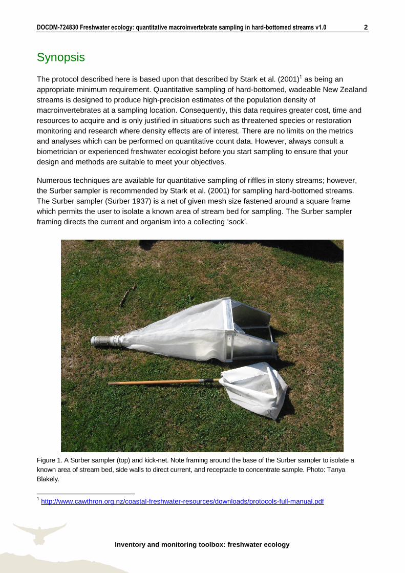
Numerous techniques are available for quantitative sampling of riffles in stony streams; however,

the Surber sampler is recommended by Stark et al. (2001) for sampling hard-bottomed streams.

The Surber sampler (Surber 1937) is a net of given mesh size fastened around a square frame

which permits the user to isolate a known area of stream bed for sampling. The Surber sampler

framing directs the current and organism into a collecting ‘sock’.

Figure 1. A Surber sampler (top) and kick-net. Note framing around the base of the Surber sampler to isolate a

known area of stream bed, side walls to direct current, and receptacle to concentrate sample. Photo: Tanya

Blakely.

1 http://www.cawthron.org.nz/coastal-freshwater-resources/downloads/protocols-full-manual.pdf

http://www.cawthron.org.nz/coastal-freshwater-resources/downloads/protocols-full-manual.pdf



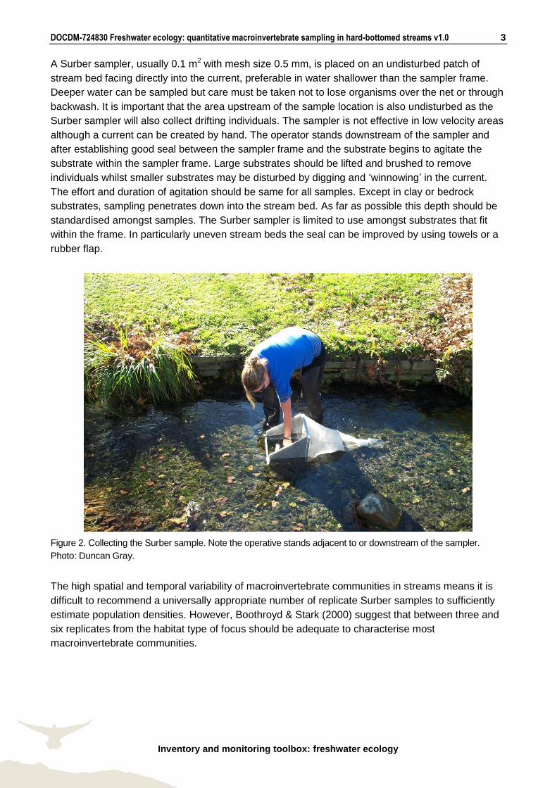
A Surber sampler, usually 0.1 m2 with mesh size 0.5 mm, is placed on an undisturbed patch of

stream bed facing directly into the current, preferable in water shallower than the sampler frame.

Deeper water can be sampled but care must be taken not to lose organisms over the net or through

backwash. It is important that the area upstream of the sample location is also undisturbed as the

Surber sampler will also collect drifting individuals. The sampler is not effective in low velocity areas

although a current can be created by hand. The operator stands downstream of the sampler and

after establishing good seal between the sampler frame and the substrate begins to agitate the

substrate within the sampler frame. Large substrates should be lifted and brushed to remove

individuals whilst smaller substrates may be disturbed by digging and ‘winnowing’ in the current.

The effort and duration of agitation should be same for all samples. Except in clay or bedrock

substrates, sampling penetrates down into the stream bed. As far as possible this depth should be

standardised amongst samples. The Surber sampler is limited to use amongst substrates that fit

within the frame. In particularly uneven stream beds the seal can be improved by using towels or a

rubber flap.

Figure 2. Collecting the Surber sample. Note the operative stands adjacent to or downstream of the sampler.

Photo: Duncan Gray.

The high spatial and temporal variability of macroinvertebrate communities in streams means it is

difficult to recommend a universally appropriate number of replicate Surber samples to sufficiently

estimate population densities. However, Boothroyd & Stark (2000) suggest that between three and

six replicates from the habitat type of focus should be adequate to characterise most

macroinvertebrate communities.



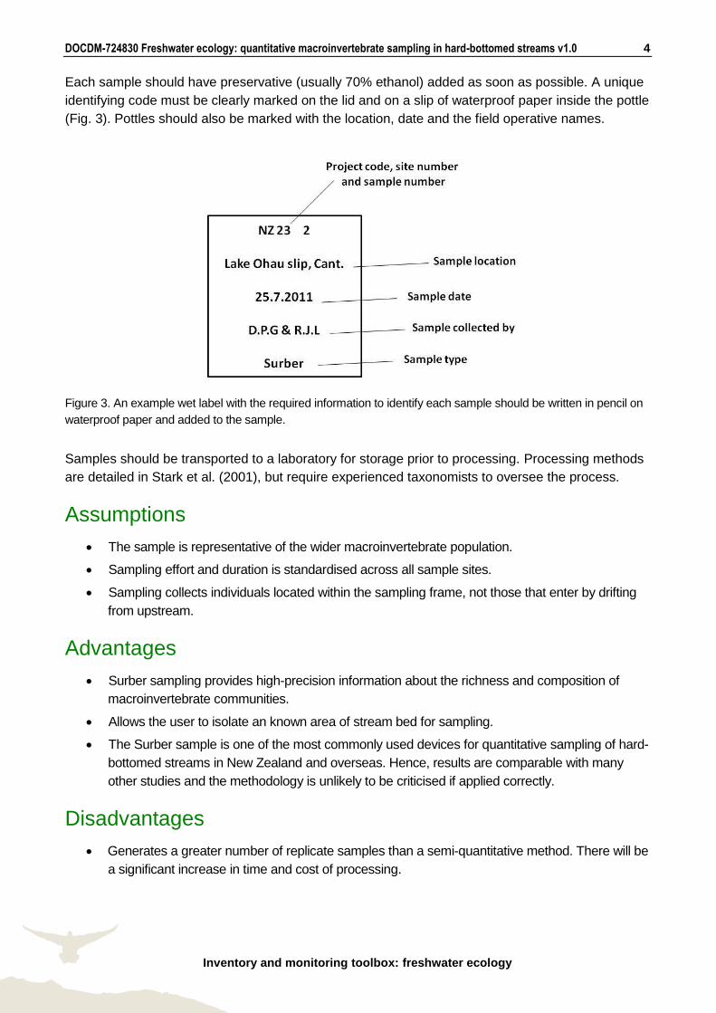
Each sample should have preservative (usually 70% ethanol) added as soon as possible. A unique

identifying code must be clearly marked on the lid and on a slip of waterproof paper inside the pottle

(Fig. 3). Pottles should also be marked with the location, date and the field operative names.

Figure 3. An example wet label with the required information to identify each sample should be written in pencil on

waterproof paper and added to the sample.

Samples should be transported to a laboratory for storage prior to processing. Processing methods

are detailed in Stark et al. (2001), but require experienced taxonomists to oversee the process.

Assumptions

The sample is representative of the wider macroinvertebrate population.

Sampling effort and duration is standardised across all sample sites.

Sampling collects individuals located within the sampling frame, not those that enter by drifting

from upstream.

Advantages

Surber sampling provides high-precision information about the richness and composition of

macroinvertebrate communities.

Allows the user to isolate an known area of stream bed for sampling.

The Surber sample is one of the most commonly used devices for quantitative sampling of hard-

bottomed streams in New Zealand and overseas. Hence, results are comparable with many

other studies and the methodology is unlikely to be criticised if applied correctly.

Disadvantages

Generates a greater number of replicate samples than a semi-quantitative method. There will be

a significant increase in time and cost of processing.



Unsuitable for deep or fast flowing streams.

Unsuitable where substrates are larger than the area of the sampler frame.

Suitability for inventory

This technique is not suitable for inventory which does not require quantitative estimates of

population size. Collection and processing of Surber samples for inventory would be a considerable

waste of time and resources and alternatively a more efficient semi-quantitative sampling or

processing method could be considered.

Suitability for monitoring

This method is suitable for monitoring where the density of individuals is considered to be of

interest. If high-precision estimates of population density are not important, consider using a more

efficient semi-quantitative sampling or processing method.

Skills

Field observers will require:

Basic training in stream macroinvertebrate and habitat sampling

Basic outdoor and river-crossing skills

A reasonable level of fitness

Study design, sample processing and quality control are specialised processes that require input

from a freshwater specialist.

Resources

Quantitative sampling of hard-bottomed streams may be carried out by a single field operative.

However, in the interests of safety it is recommended that sampling is done by teams of at least two

people.

Standard equipment includes:

Waterproof notebook or field data sheets

Pencil

Permanent marker pen

Wet labels

Waders or gumboots, dependent on stream depth

GPS and map



Specialist equipment required:

Surber sampler (0.1 m2, 0.5 mm mesh)

White tray or 10 litre bucket

Sieve or sieve bucket

Plastic sample containers (usually 500–1000 ml volume)

Preservative (usually 70% ethanol)

Minimum attributes

Consistent measurement and recording of these attributes is critical for the implementation of the

method. Other attributes may be optional depending on your objective. For more information refer

to ‘Full details of technique and best practice’.

DOC staff must complete a ‘Standard inventory and monitoring project plan’ (docdm-146272).

The more information that is collected at each site, the more thorough and complete will be any

interpretation of the biological data collected. However, some basic information should be recorded

with each sample collected:

Substrate composition

Riparian vegetation

Stream width

Stream depth

Stream velocity

Periphyton community composition

It is also commonplace to collect basic water chemistry information where possible. Temperature

(°C), electrical conductivity (µS), pH and dissolved oxygen may all be measured by handheld

meters to inform biological data. Some habitat and sites notes are also worthwhile, e.g. the

occurrence of stock at the site or evidence of recent flooding. The ‘Stream habitat assessment field

sheet’ (docdm-761873) is a good guide to the basic information that can be collected without

recourse to specialised equipment or processing in a laboratory. Basic training in the use of this

habitat sheet and/or a thorough perusal of Harding et al. (2009) is required before use of this habitat

assessment sheet.2 As with all visual and qualitative assessments it is important to standardise

collection protocols within a group of field observers or within a particular project. There is

considerable opportunity for user bias with this method of habitat assessment.

2 http://www.cawthron.org.nz/coastal-freshwater-resources/downloads/stream-habitat-assessment-

protocols.pdf

http://www.doc.govt.nz/Documents/science-and-technical/inventory-monitoring/im-toolbox-freshwater-ecology/im-toolbox-freshwater-ecology-stream-habitat-assessment-field-sheet.pdf

http://www.doc.govt.nz/Documents/science-and-technical/inventory-monitoring/im-toolbox-freshwater-ecology/im-toolbox-freshwater-ecology-stream-habitat-assessment-field-sheet.pdf

http://www.cawthron.org.nz/coastal-freshwater-resources/downloads/stream-habitat-assessment-protocols.pdf




Data storage

If data storage is designed well at the outset, it will make the job of analysis and interpretation much

easier. Before storing data, check for missing information and errors, and ensure metadata are

recorded. Forward copies of completed field survey sheets to the survey administrator, or enter

data into an appropriate spreadsheet as soon as possible. The key steps are data entry, storage

and data checking/quality assurance for later analysis, followed by copying and data backup for

security.

It is quite likely that biological sample processing will be outsourced to an accredited laboratory.

During sample processing, data is conventionally recorded on a hardcopy data sheet prior to

transfer to an electronic format. Hardcopy sheets will be clearly marked with the details of the

project and identity of samples. The format of hardcopy data sheets is normally columns

representing samples and rows for each species or taxa group. Data should be entered into an

electronic media in the same format to avoid confusion (see ‘Stream invertebrate data sheet

example’—docdm-761858). Electronic data sheets should contain all the information required to

identify each sample, and any habitat or water chemistry data that was collected simultaneously

may be appended on a separate worksheet within the electronic file (usually Excel).

It is important that habitat and water chemistry data are entered in a comparable format to biological

data, i.e. columns as sites, and this should be done as soon as possible by the field operative so

that details are fresh. All hardcopies of habitat data and notes should be labelled and stored in a

project file and retained.

All electronic files should have a notes sheet which details any relevant information for future users.

In particular each user, beginning with the field operative who enters the data, should record details

of any changes to the data, including when and why they were made. It is also recommended to

retain a single version of the data which has undergone quality control and may not be altered. All

analysis is performed on copies of this master sheet.

Forward copies of completed survey sheets to the survey administrator, or enter data into an

appropriate spreadsheet as soon as possible. Collate, consolidate and store survey information

securely, also as soon as possible, and preferably immediately on return from the field. The key

steps here are data entry, storage and maintenance for later analysis, followed by copying and data

backup for security.

Summarise the results in a spreadsheet or equivalent. Arrange data as ‘column variables’—i.e.

arrange data from each field on the data sheet (date, time, location, plot designation, number seen,

identity, etc.) in columns, with each row representing the occasion on which a given survey plot was

sampled.

If data storage is designed well at the outset, it will make the job of analysis and interpretation much

easier. Before storing data, check for missing information and errors, and ensure metadata are

recorded.



Storage tools can be either manual or electronic systems (or both, preferably). They will usually be

summary sheets, other physical filing systems, or electronic spreadsheets and databases. Use

appropriate file formats such as .xls, .txt, .dbf or specific analysis software formats. Copy and/or

backup all data, whether electronic, data sheets, metadata or site access descriptions, preferably

offline if the primary storage location is part of a networked system. Store the copy at a separate

location for security purposes.

Analysis, interpretation and reporting

Seek statistical advice from a biometrician or suitably experienced person prior to undertaking any

analysis.

The invertebrate data derived from Surber sampling are either semi-quantitative fixed counts or

more commonly full counts of all individuals. They are high-precision estimates of population size.

There is no limit to the indices or analyses that can be produced with this data. Common basic

indices calculated from this data are:

Taxa richness

Richness of Ephemeroptera, Plecoptera and Trichoptera (EPT) taxa or % EPT abundance

Macroinvertebrate Community suite of indices, especially the Quantitative Macroinvertebrate

Community Index (QMCI) (Stark 1985)

Taxa richness

Taxa richness is simply the number of taxa that were found at a site and is most commonly used for

inventory or ecosystem condition monitoring. Sites may be compared in terms of taxa richness

provided the sampling effort and taxonomic resolution at each site is standardised. If groups of sites

are to be compared, e.g. forest streams versus grassland streams, then it is important that equal

numbers of each site type have been sampled. If this assumption is violated the degree of

difference must be noted or comparisons will require rarefaction and a biometrician should be

consulted (Magurran 2004). If sample numbers and effort are balanced, i.e. equal, then basic

Analyses of Variance (ANOVA) or t-tests can be used to compare between the mean values for

habitat types. Alternatively, instead of comparing richness between groups, a gradient approach

may be used whereby the richness of taxa at each site is compared to the value for an

environmental condition at that site. Such a correlative approach is more appropriate when sites do

not fit into meaningful groupings.

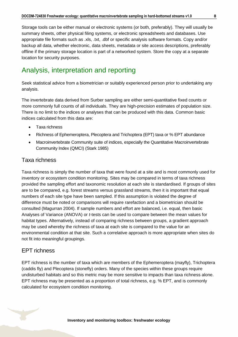
EPT richness

EPT richness is the number of taxa which are members of the Ephemeroptera (mayfly), Trichoptera

(caddis fly) and Plecoptera (stonefly) orders. Many of the species within these groups require

undisturbed habitats and so this metric may be more sensitive to impacts than taxa richness alone.

EPT richness may be presented as a proportion of total richness, e.g. % EPT, and is commonly

calculated for ecosystem condition monitoring.



MCI

The Macroinvertebrate Community Index (MCI) was initially proposed by Stark (1985) to assess

organic enrichment in the stony riffles of New Zealand streams and rivers. However, despite

criticisms, it has proven to be an effective measure of the effects of a number of different impacts

on stream invertebrate communities and is regularly used in ecosystem condition monitoring. Each

taxa is assigned a score (1–10) which represents its tolerance to pollution. The MCI score for a

sample is calculated thus:

= 20 ∑ ai / S

Where ai is the MCI tolerance score for the ith taxon and S is the total number of taxa. Taxon

tolerance scores can be found in Table 3.

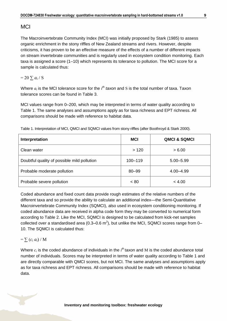
MCI values range from 0–200, which may be interpreted in terms of water quality according to

Table 1. The same analyses and assumptions apply as for taxa richness and EPT richness. All

comparisons should be made with reference to habitat data.

Table 1. Interpretation of MCI, QMCI and SQMCI values from stony riffles (after Boothroyd & Stark 2000).

Interpretation MCI QMCI & SQMCI

Clean water > 120 > 6.00

Doubtful quality of possible mild pollution 100–119 5.00–5.99

Probable moderate pollution 80–99 4.00–4.99

Probable severe pollution < 80 < 4.00

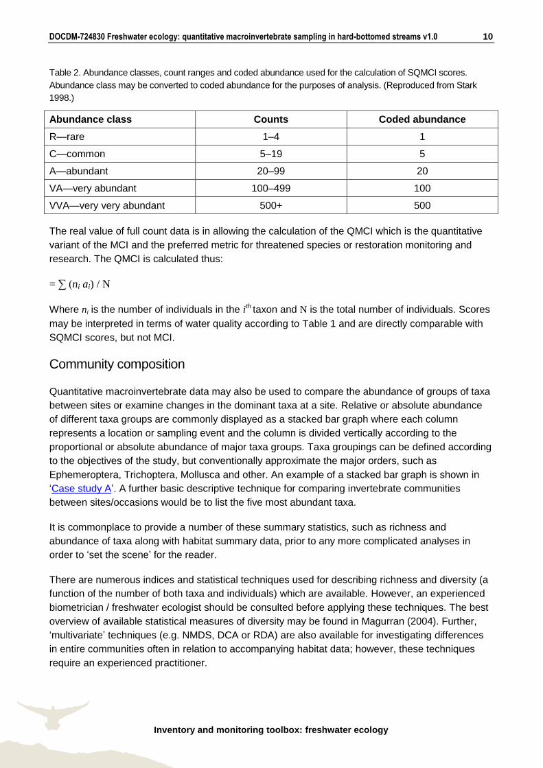
Coded abundance and fixed count data provide rough estimates of the relative numbers of the

different taxa and so provide the ability to calculate an additional index—the Semi-Quantitative

Macroinvertebrate Community Index (SQMCI), also used in ecosystem conditioning monitoring. If

coded abundance data are received in alpha code form they may be converted to numerical form

according to Table 2. Like the MCI, SQMCI is designed to be calculated from kick-net samples

collected over a standardised area (0.3–0.6 m2), but unlike the MCI, SQMCI scores range from 0–

10. The SQMCI is calculated thus:

= ∑ (ci ai) / M

Where ci is the coded abundance of individuals in the ith taxon and M is the coded abundance total

number of individuals. Scores may be interpreted in terms of water quality according to Table 1 and

are directly comparable with QMCI scores, but not MCI. The same analyses and assumptions apply

as for taxa richness and EPT richness. All comparisons should be made with reference to habitat

data.



Table 2. Abundance classes, count ranges and coded abundance used for the calculation of SQMCI scores.

Abundance class may be converted to coded abundance for the purposes of analysis. (Reproduced from Stark

1998.)

Abundance class Counts Coded abundance

R—rare 1–4 1

C—common 5–19 5

A—abundant 20–99 20

VA—very abundant 100–499 100

VVA—very very abundant 500+ 500

The real value of full count data is in allowing the calculation of the QMCI which is the quantitative

variant of the MCI and the preferred metric for threatened species or restoration monitoring and

research. The QMCI is calculated thus:

= ∑ (ni ai) / N

Where ni is the number of individuals in the ith taxon and N is the total number of individuals. Scores

may be interpreted in terms of water quality according to Table 1 and are directly comparable with

SQMCI scores, but not MCI.

Community composition

Quantitative macroinvertebrate data may also be used to compare the abundance of groups of taxa

between sites or examine changes in the dominant taxa at a site. Relative or absolute abundance

of different taxa groups are commonly displayed as a stacked bar graph where each column

represents a location or sampling event and the column is divided vertically according to the

proportional or absolute abundance of major taxa groups. Taxa groupings can be defined according

to the objectives of the study, but conventionally approximate the major orders, such as

Ephemeroptera, Trichoptera, Mollusca and other. An example of a stacked bar graph is shown in

‘Case study A’. A further basic descriptive technique for comparing invertebrate communities

between sites/occasions would be to list the five most abundant taxa.

It is commonplace to provide a number of these summary statistics, such as richness and

abundance of taxa along with habitat summary data, prior to any more complicated analyses in

order to ‘set the scene’ for the reader.

There are numerous indices and statistical techniques used for describing richness and diversity (a

function of the number of both taxa and individuals) which are available. However, an experienced

biometrician / freshwater ecologist should be consulted before applying these techniques. The best

overview of available statistical measures of diversity may be found in Magurran (2004). Further,

‘multivariate’ techniques (e.g. NMDS, DCA or RDA) are also available for investigating differences

in entire communities often in relation to accompanying habitat data; however, these techniques

require an experienced practitioner.



The majority of collation and calculation described here can be performed in a basic spreadsheet

package such as Excel, although there are a variety of commercial and freeware packages

available to calculate summary statistics and perform more in-depth analyses. However, beyond the

basic descriptive statistics, such as richness, MCI and summary plots, the user will require specific

training and experience.

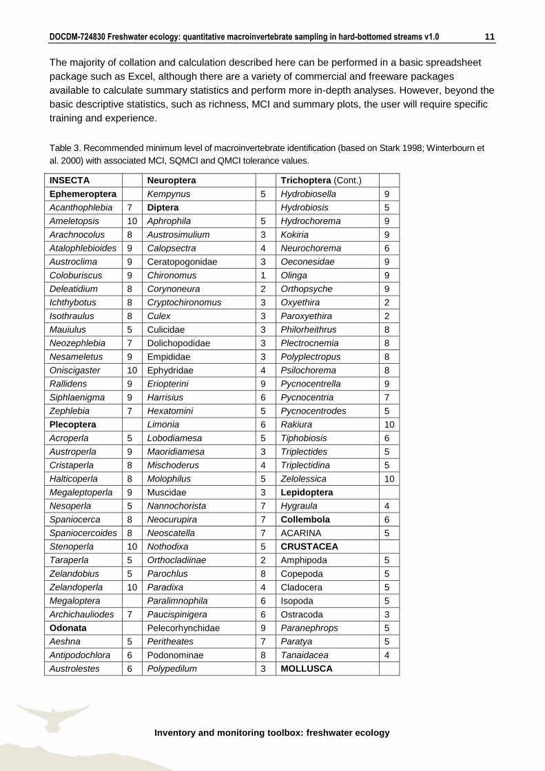
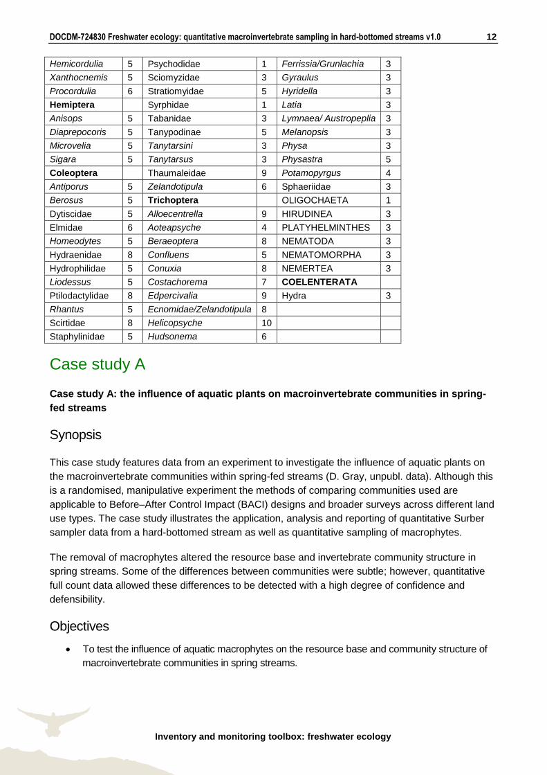
Table 3. Recommended minimum level of macroinvertebrate identification (based on Stark 1998; Winterbourn et

al. 2000) with associated MCI, SQMCI and QMCI tolerance values.

INSECTA Neuroptera Trichoptera (Cont.)

Ephemeroptera Kempynus 5 Hydrobiosella 9

Acanthophlebia 7 Diptera Hydrobiosis 5

Ameletopsis 10 Aphrophila 5 Hydrochorema 9

Arachnocolus 8 Austrosimulium 3 Kokiria 9

Atalophlebioides 9 Calopsectra 4 Neurochorema 6

Austroclima 9 Ceratopogonidae 3 Oeconesidae 9

Coloburiscus 9 Chironomus 1 Olinga 9

Deleatidium 8 Corynoneura 2 Orthopsyche 9

Ichthybotus 8 Cryptochironomus 3 Oxyethira 2

Isothraulus 8 Culex 3 Paroxyethira 2

Mauiulus 5 Culicidae 3 Philorheithrus 8

Neozephlebia 7 Dolichopodidae 3 Plectrocnemia 8

Nesameletus 9 Empididae 3 Polyplectropus 8

Oniscigaster 10 Ephydridae 4 Psilochorema 8

Rallidens 9 Eriopterini 9 Pycnocentrella 9

Siphlaenigma 9 Harrisius 6 Pycnocentria 7

Zephlebia 7 Hexatomini 5 Pycnocentrodes 5

Plecoptera Limonia 6 Rakiura 10

Acroperla 5 Lobodiamesa 5 Tiphobiosis 6

Austroperla 9 Maoridiamesa 3 Triplectides 5

Cristaperla 8 Mischoderus 4 Triplectidina 5

Halticoperla 8 Molophilus 5 Zelolessica 10

Megaleptoperla 9 Muscidae 3 Lepidoptera

Nesoperla 5 Nannochorista 7 Hygraula 4

Spaniocerca 8 Neocurupira 7 Collembola 6

Spaniocercoides 8 Neoscatella 7 ACARINA 5

Stenoperla 10 Nothodixa 5 CRUSTACEA

Taraperla 5 Orthocladiinae 2 Amphipoda 5

Zelandobius 5 Parochlus 8 Copepoda 5

Zelandoperla 10 Paradixa 4 Cladocera 5

Megaloptera Paralimnophila 6 Isopoda 5

Archichauliodes 7 Paucispinigera 6 Ostracoda 3

Odonata Pelecorhynchidae 9 Paranephrops 5

Aeshna 5 Peritheates 7 Paratya 5

Antipodochlora 6 Podonominae 8 Tanaidacea 4

Austrolestes 6 Polypedilum 3 MOLLUSCA



Hemicordulia 5 Psychodidae 1 Ferrissia/Grunlachia 3

Xanthocnemis 5 Sciomyzidae 3 Gyraulus 3

Procordulia 6 Stratiomyidae 5 Hyridella 3

Hemiptera Syrphidae 1 Latia 3

Anisops 5 Tabanidae 3 Lymnaea/ Austropeplia 3

Diaprepocoris 5 Tanypodinae 5 Melanopsis 3

Microvelia 5 Tanytarsini 3 Physa 3

Sigara 5 Tanytarsus 3 Physastra 5

Coleoptera Thaumaleidae 9 Potamopyrgus 4

Antiporus 5 Zelandotipula 6 Sphaeriidae 3

Berosus 5 Trichoptera OLIGOCHAETA 1

Dytiscidae 5 Alloecentrella 9 HIRUDINEA 3

Elmidae 6 Aoteapsyche 4 PLATYHELMINTHES 3

Homeodytes 5 Beraeoptera 8 NEMATODA 3

Hydraenidae 8 Confluens 5 NEMATOMORPHA 3

Hydrophilidae 5 Conuxia 8 NEMERTEA 3

Liodessus 5 Costachorema 7 COELENTERATA

Ptilodactylidae 8 Edpercivalia 9 Hydra 3

Rhantus 5 Ecnomidae/Zelandotipula 8

Scirtidae 8 Helicopsyche 10

Staphylinidae 5 Hudsonema 6

Case study A

Case study A: the influence of aquatic plants on macroinvertebrate communities in spring-

fed streams

Synopsis

This case study features data from an experiment to investigate the influence of aquatic plants on

the macroinvertebrate communities within spring-fed streams (D. Gray, unpubl. data). Although this

is a randomised, manipulative experiment the methods of comparing communities used are

applicable to Before–After Control Impact (BACI) designs and broader surveys across different land

use types. The case study illustrates the application, analysis and reporting of quantitative Surber

sampler data from a hard-bottomed stream as well as quantitative sampling of macrophytes.

The removal of macrophytes altered the resource base and invertebrate community structure in

spring streams. Some of the differences between communities were subtle; however, quantitative

full count data allowed these differences to be detected with a high degree of confidence and

defensibility.

Objectives

To test the influence of aquatic macrophytes on the resource base and community structure of

macroinvertebrate communities in spring streams.



Sampling design and methods

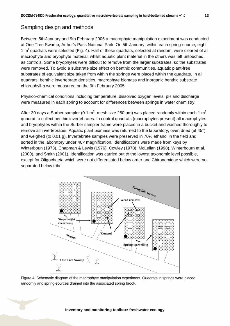
Between 5th January and 9th February 2005 a macrophyte manipulation experiment was conducted

at One Tree Swamp, Arthur’s Pass National Park. On 5th January, within each spring-source, eight

1 m2 quadrats were selected (Fig. 4). Half of these quadrats, selected at random, were cleared of all

macrophyte and bryophyte material, whilst aquatic plant material in the others was left untouched,

as controls. Some bryophytes were difficult to remove from the larger substrates, so the substrates

were removed. To avoid a substrate size effect on benthic communities, aquatic plant-free

substrates of equivalent size taken from within the springs were placed within the quadrats. In all

quadrats, benthic invertebrate densities, macrophyte biomass and inorganic benthic substrate

chlorophyll-a were measured on the 9th February 2005.

Physico-chemical conditions including temperature, dissolved oxygen levels, pH and discharge

were measured in each spring to account for differences between springs in water chemistry.

After 30 days a Surber sampler (0.1 m2, mesh size 250 µm) was placed randomly within each 1 m2

quadrat to collect benthic invertebrates. In control quadrats (macrophytes present) all macrophytes

and bryophytes within the Surber sampler frame were placed in a bucket and washed thoroughly to

remove all invertebrates. Aquatic plant biomass was returned to the laboratory, oven dried (at 45°)

and weighed (to 0.01 g). Invertebrate samples were preserved in 70% ethanol in the field and

sorted in the laboratory under 40× magnification. Identifications were made from keys by

Winterboun (1973), Chapman & Lewis (1976), Cowley (1978), McLellan (1998), Winterbourn et al.

(2000), and Smith (2001). Identification was carried out to the lowest taxonomic level possible,

except for Oligochaeta which were not differentiated below order and Chironomidae which were not

separated below tribe.

Stream

Stage height

recorders

Floodplain terrace

Weed removal

Control

One Tree Swamp

Spring up-welling

Figure 4. Schematic diagram of the macrophyte manipulation experiment. Quadrats in springs were placed

randomly and spring-sources drained into the associated spring brook.



At the end of the experiment periphyton biomass (organic layers on the stone surfaces), within

control and treatment quadrats, was estimated by measuring chlorophyll-a. Three stones devoid of

macrophytes or bryophytes were randomly collected from each quadrat, within each treatment, and

were placed in 100 ml of 90% ethanol for 24 hours at 4°C in the dark. Periphyton biomass was

estimated using standard techniques.

The statistical techniques used to analyse this data are specific to the design and objectives of this

study and are not detailed here. Experimental design and analysis is a highly specialised process

and an experienced biometrician or ecologist should be consulted both before and after field work is

carried out.

Results

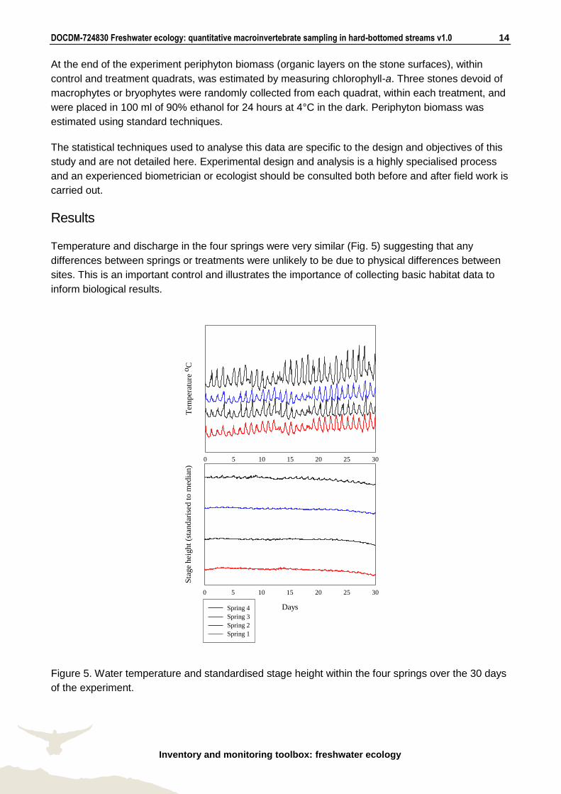
Temperature and discharge in the four springs were very similar (Fig. 5) suggesting that any

differences between springs or treatments were unlikely to be due to physical differences between

sites. This is an important control and illustrates the importance of collecting basic habitat data to

inform biological results.

0 5 10 15 20 25 30

Tem

per

ature

oC

Days

0 5 10 15 20 25 30

Sta

ge

hei

ght

(sta

ndar

ised

to m

edia

n)

Spring 4

Spring 3

Spring 2

Spring 1

Figure 5. Water temperature and standardised stage height within the four springs over the 30 days

of the experiment.



Periphyton biomass

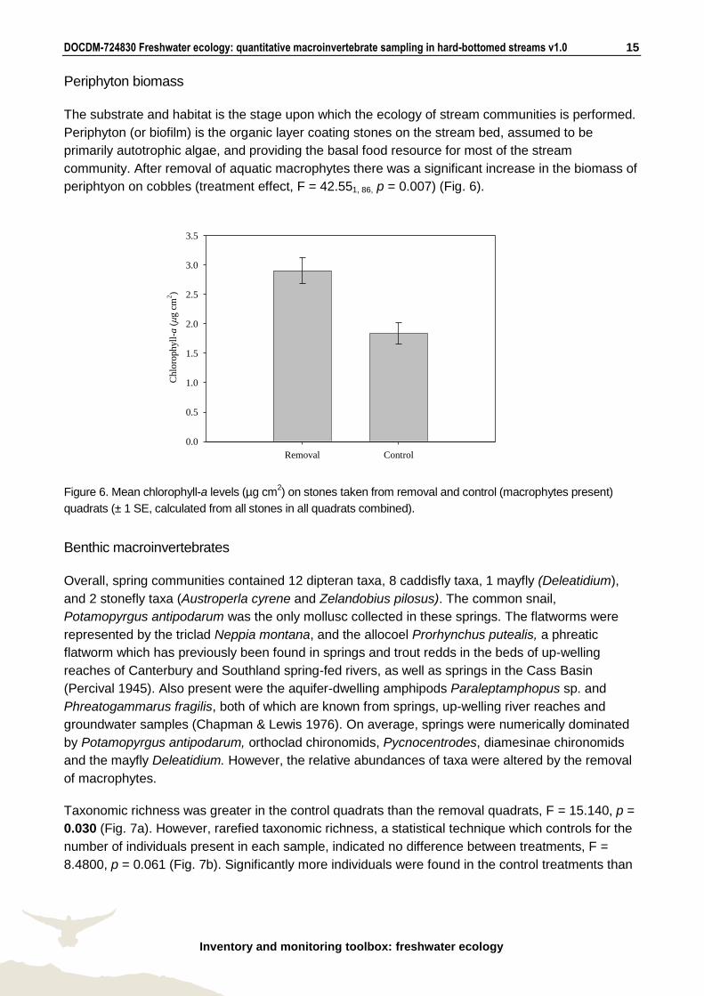
The substrate and habitat is the stage upon which the ecology of stream communities is performed.

Periphyton (or biofilm) is the organic layer coating stones on the stream bed, assumed to be

primarily autotrophic algae, and providing the basal food resource for most of the stream

community. After removal of aquatic macrophytes there was a significant increase in the biomass of

periphtyon on cobbles (treatment effect, F = 42.551, 86, p = 0.007) (Fig. 6).

Removal Control

Chlo

rophyll

-a (

g c

m2)

0.0

0.5

1.0

1.5

2.0

2.5

3.0

3.5

Figure 6. Mean chlorophyll-a levels (µg cm2) on stones taken from removal and control (macrophytes present)

quadrats (± 1 SE, calculated from all stones in all quadrats combined).

Benthic macroinvertebrates

Overall, spring communities contained 12 dipteran taxa, 8 caddisfly taxa, 1 mayfly (Deleatidium),

and 2 stonefly taxa (Austroperla cyrene and Zelandobius pilosus). The common snail,

Potamopyrgus antipodarum was the only mollusc collected in these springs. The flatworms were

represented by the triclad Neppia montana, and the allocoel Prorhynchus putealis, a phreatic

flatworm which has previously been found in springs and trout redds in the beds of up-welling

reaches of Canterbury and Southland spring-fed rivers, as well as springs in the Cass Basin

(Percival 1945). Also present were the aquifer-dwelling amphipods Paraleptamphopus sp. and

Phreatogammarus fragilis, both of which are known from springs, up-welling river reaches and

groundwater samples (Chapman & Lewis 1976). On average, springs were numerically dominated

by Potamopyrgus antipodarum, orthoclad chironomids, Pycnocentrodes, diamesinae chironomids

and the mayfly Deleatidium. However, the relative abundances of taxa were altered by the removal

of macrophytes.

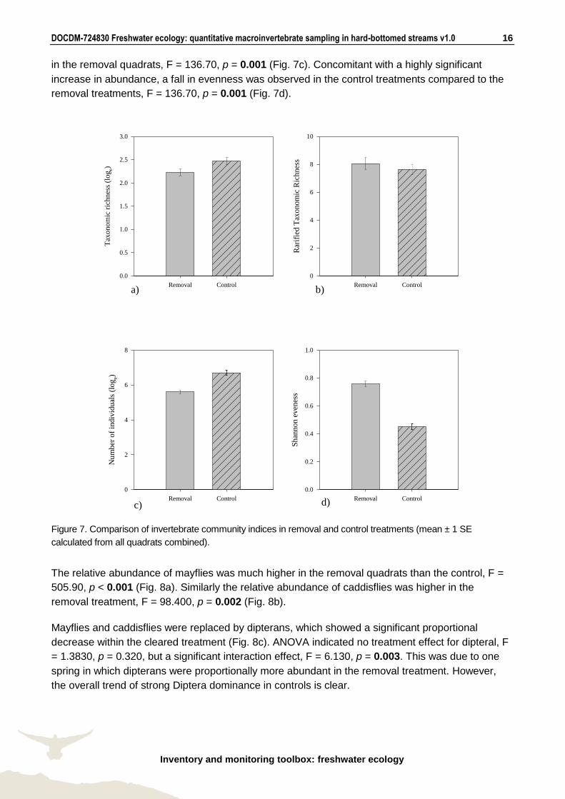
Taxonomic richness was greater in the control quadrats than the removal quadrats, F = 15.140, p =

0.030 (Fig. 7a). However, rarefied taxonomic richness, a statistical technique which controls for the

number of individuals present in each sample, indicated no difference between treatments, F =

8.4800, p = 0.061 (Fig. 7b). Significantly more individuals were found in the control treatments than



in the removal quadrats, F = 136.70, p = 0.001 (Fig. 7c). Concomitant with a highly significant

increase in abundance, a fall in evenness was observed in the control treatments compared to the

removal treatments, F = 136.70, p = 0.001 (Fig. 7d).

Removal Control

Tax

onom

ic r

ichnes

s (l

og

e)

0.0

0.5

1.0

1.5

2.0

2.5

3.0

Removal Control

Rar

ifie

d T

axonom

ic R

ichnes

s

0

2

4

6

8

10

Removal Control

Num

ber

of

indiv

idual

s (l

og

e)

0

2

4

6

8

Removal Control

Shan

non e

ven

ess

0.0

0.2

0.4

0.6

0.8

1.0

a) b)

c) d)

e) f)

Figure 7. Comparison of invertebrate community indices in removal and control treatments (mean ± 1 SE

calculated from all quadrats combined).

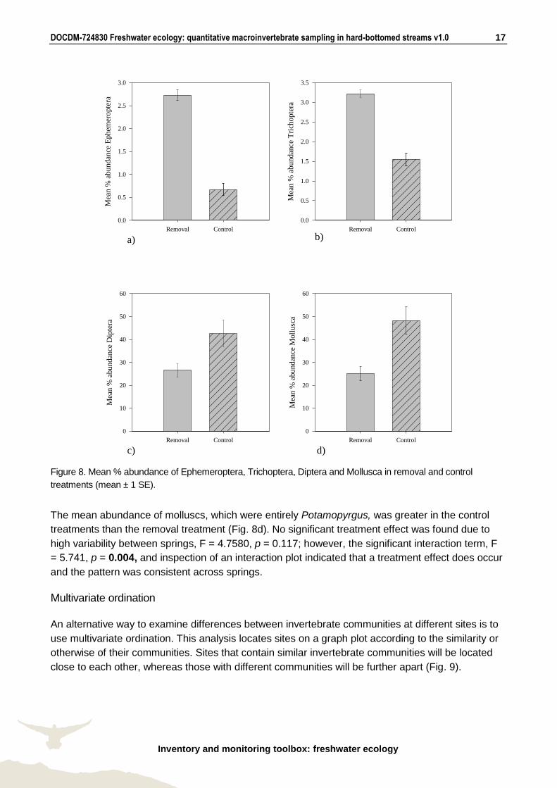
The relative abundance of mayflies was much higher in the removal quadrats than the control, F =

505.90, p < 0.001 (Fig. 8a). Similarly the relative abundance of caddisflies was higher in the

removal treatment, F = 98.400, p = 0.002 (Fig. 8b).

Mayflies and caddisflies were replaced by dipterans, which showed a significant proportional

decrease within the cleared treatment (Fig. 8c). ANOVA indicated no treatment effect for dipteral, F

= 1.3830, p = 0.320, but a significant interaction effect, F = 6.130, p = 0.003. This was due to one

spring in which dipterans were proportionally more abundant in the removal treatment. However,

the overall trend of strong Diptera dominance in controls is clear.



Removal Control

Mea

n %

abundan

ce D

ipte

ra

0

10

20

30

40

50

60

Removal Control

Mea

n %

abundan

ce M

oll

usc

a

0

10

20

30

40

50

60

Removal Control

Mea

n %

abundan

ce E

phem

eropte

ra

0.0

0.5

1.0

1.5

2.0

2.5

3.0

Removal Control

Mea

n %

abundan

ce T

rich

opte

ra

0.0

0.5

1.0

1.5

2.0

2.5

3.0

3.5

a) b)

c) d)

Figure 8. Mean % abundance of Ephemeroptera, Trichoptera, Diptera and Mollusca in removal and control

treatments (mean ± 1 SE).

The mean abundance of molluscs, which were entirely Potamopyrgus, was greater in the control

treatments than the removal treatment (Fig. 8d). No significant treatment effect was found due to

high variability between springs, F = 4.7580, p = 0.117; however, the significant interaction term, F

= 5.741, p = 0.004, and inspection of an interaction plot indicated that a treatment effect does occur

and the pattern was consistent across springs.

Multivariate ordination

An alternative way to examine differences between invertebrate communities at different sites is to

use multivariate ordination. This analysis locates sites on a graph plot according to the similarity or

otherwise of their communities. Sites that contain similar invertebrate communities will be located

close to each other, whereas those with different communities will be further apart (Fig. 9).



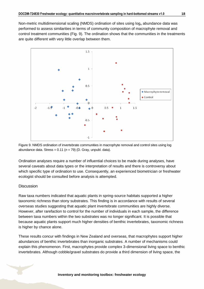
Non-metric multidimensional scaling (NMDS) ordination of sites using loge abundance data was

performed to assess similarities in terms of community composition of macrophyte removal and

control treatment communities (Fig. 9). The ordination shows that the communities in the treatments

are quite different with very little overlap between them.

Figure 9. NMDS ordination of invertebrate communities in macrophyte removal and control sites using log

abundance data. Stress = 0.11 (n = 79) (D. Gray, unpubl. data).

Ordination analyses require a number of influential choices to be made during analyses, have

several caveats about data types or the interpretation of results and there is controversy about

which specific type of ordination to use. Consequently, an experienced biometrician or freshwater

ecologist should be consulted before analysis is attempted.

Discussion

Raw taxa numbers indicated that aquatic plants in spring-source habitats supported a higher

taxonomic richness than stony substrates. This finding is in accordance with results of several

overseas studies suggesting that aquatic plant invertebrate communities are highly diverse.

However, after rarefaction to control for the number of individuals in each sample, the difference

between taxa numbers within the two substrates was no longer significant. It is possible that

because aquatic plants support much higher densities of benthic invertebrates, taxonomic richness

is higher by chance alone.

These results concur with findings in New Zealand and overseas, that macrophytes support higher

abundances of benthic invertebrates than inorganic substrates. A number of mechanisms could

explain this phenomenon. First, macrophytes provide complex 3-dimensional living space to benthic

invertebrates. Although cobble/gravel substrates do provide a third dimension of living space, the



hyporheic zone is often not sampled by conventional techniques, e.g. a Surber sampler.

Macrophyte beds extend available habitat up into the water column and therefore equate to a larger

volume of habitat than is sampled by conventional techniques. Secondly, macrophyte and

bryophyte beds provide protection from de-faunating flow velocities. This allows the density of

invertebrates able to live on aquatic plants to reach high levels. Furthermore, aquatic plant

communities have been shown to be depauperate in predatory taxa. Finally, the high abundance of

benthic invertebrates within aquatic plant beds were probably supported by elevated levels of food

resources. Living macrophytes and bryophytes rarely provide a direct source of food for New

Zealand benthic invertebrates, but epilithon and detritus that collects on them are a constant source

of food. Thus, it is likely that invertebrate abundance on aquatic plants was enhanced by the

increased living space they provide, benign flow conditions, relatively low levels of predation and

high food resource availability.

The shift in community composition and dominance of quadrats from chironomids and molluscs in

control quadrats to mayflies and caddis in removal quadrats is consistent with our understanding of

the ecology of these taxa. Deleatidium and the cased caddisflies Pycnocentrodes and Pycnocentria

are predominantly stone-surface grazers, which ingest algal periphyton, and detritus that becomes

entrained within the algae on stone surfaces. The lack of light below aquatic plant beds significantly

reduced levels of periphyton on stones, and therefore, the algal food resources of mayflies and

caddisflies. Conversely, the protection from high flows and predation, plus the possibility of

enhanced levels of epilithon and organic matter retention on the aquatic plants themselves, provide

conditions more suitable for mollusc and chironomid taxa that may be more capable of negotiating

the complex architecture of plants.

Limitations and points to consider

Surber sampling allowed subtle changes in the composition of macroinvertebrate communities

to be examined. This would not have been possible using semi-quantitative data.

Due in part to the intensity of sampling, the spatial spread of this comparison is reduced.

Consequently caution must be exercised when extrapolating these results to other stream

systems. To test generalities it is not unusual to link a broadscale semi-quantitative survey with

more focused small-scale quantitative sampling.

As in all situations the objectives dictate the methods used. Revisit the ‘Decision tree’ in the

‘Introduction to macroinvertebrate monitoring in freshwater ecosystems’ (docdm-724991) to

confirm you have chosen the correct path.

References for case study A

Chapman, A.; Lewis, M. 1976: An introduction to the freshwater Crustacea of New Zealand. Collins,

Auckland. 261 p.

Cowley, D.R. 1978: Studies on the larvae of New Zealand Trichoptera. New Zealand Journal of Zoology

5: 639–750.



McLellan, I.D. 1998: A revision of Acroperla (Plecoptera: Zelandoperlinae) and removal of species to

Taraperla new genus. New Zealand of Zoology 25: 185–203.

Percival, E. 1945: The genus Prorhynchus in New Zealand. Transactions of the Royal Society of New

Zealand 75: 33–41.

Smith, B.J. 2001: Larval Hydrobiosidae. Biodiversity identification workshop. National Institute of Water

and Atmospheric Research, Christchurch.

Winterbourn, M.J. 1973: A guide to the freshwater Mollusca of New Zealand. Tuatara 20: 141–159.

Winterbourn, M.J.; Gregson, K.L.D.; Dolphin, C.H. 2000: Guide to the aquatic insects of New Zealand.

Bulletin of the Entomological Society of New Zealand 13.

Full details of technique and best practice

A complete and detailed guide to this technique can be found in Stark et al. (2001).

Protocol:

1. Ensure that the sampling net is clean.

2. Select a suitable sample reach and habitat (e.g. riffle). Sample beginning at the downstream

end of the reach and proceeding across and upstream.

3. Place the sampler on the streambed ensuring a good fit around the perimeter. The sampler

should be positioned so that the water current washes dislodged material into the net.

4. Brush material from the upper surface of all cobbles contained within the sample quadrat.

Pick up each cobble and, holding it immediately in front of the net mouth, brush all sides of

the cobble clean. Repeat for all of the larger substrate elements within the sampler

quadrate. Place clean cobbles outside of the sampler quadrat. Disturb the finer substrate

remaining within the quadrate to a depth of 5–10 cm. Beware of broken glass and other

sharp objects.

5. Remove the sampler from the water, rinse the net several times to concentrate the sample

in the bottom of the net (take care not to lose material during this process), and return to the

stream bank. Remove and discard large substrate elements that may have entered the net,

taking care to remove adhering invertebrates before disposal. Remove sample from

collection net either by inverting net into a suitable container, or by removing container

attached to end of collection net. Elutriation may also be required (i.e. repeated rinsing of

sample to separate organic and inorganic fractions).

6. Let the sample settle for a few minutes and decant off excess water via the sieve. Return

any macroinvertebrates that are washed out with the water to the sample container.

(Tweezers may be useful here.)

7. Add preservative. Aim for a preservative concentration in the sample container of 70–80%

(i.e. allowing for the water already present). Be generous with preservative for samples

containing plant material (leaves, sticks, macrophytes, moss or periphyton).



8. Place a sticky label on the side of the sample container and record the side code/name,

date and replicate number (if applicable) using a permanent marker. Write on the label when

it is dry and do not rely on a label on the pottle lid! Place a waterproof label inside the

container. Screw the lid on tightly.

9. Note the sample type (e.g. Surber 0.1 m2), collector’s name and preservative used on the

field data sheet.

References and further reading

Boothroyd, I.K.G.; Stark, J.D. 2000: Use of invertebrates in monitoring. Pp. 344–373 in Collier, K.J.;

Winterbourn, M.J. (Eds): New Zealand stream invertebrates: ecology and implications for

management. New Zealand Limnological Society, Christchurch.

Harding, J.S.; Clapcott, J.; Quinn, J.; Hayes, J.; Joy, M.; Storey, R.; Greig, H.; Hay, J.; James, T.;

Beech, M.; Ozane, R.; Meredith, A.; Boothroyd, I. 2009: Stream habitat assessment protocols

for wadeable rivers and streams of New Zealand. University of Canterbury, Christchurch.

http://www.cawthron.org.nz/coastal-freshwater-resources/downloads/stream-habitat-

assessment-protocols.pdf

Stark, J.D. 1985: A macroinvertebrate community index of water quality for stony streams. Water & Soil

Miscellaneous Publication 87. National Water and Soil Conservation Authority, Wellington.

Stark, J.D. 1998: SQMCI: a biotic index for freshwater macroinvertebrate coded abundance data. New

Zealand Journal of Marine and Freshwater Research 32: 55–66.

Stark, J.D.; Boothroyd, I.K.G.; Harding, J.S.; Maxted, J.R.; Scarsbrook, M.R. 2001: Protocols for

sampling macroinvertebrates in wadeable streams. Prepared for the Ministry for the

Environment, Sustainable Management Fund Project No. 5103.


Surber, E.W. 1937: Rainbow trout and bottom fauna production in one mile of stream. Transactions of

the American Fisheries Society 66: 193–202.

Winterbourn, M.J.; Gregson, K.L.D.; Dolphin, C.H. 2000: Guide to the aquatic insects of New Zealand.

Bulletin of the Entomological Society of New Zealand 13.





Appendix A

The following Department of Conservation documents are referred to in this method:

docdm-724991 Introduction to macroinvertebrate monitoring in freshwater ecosystems

docdm-146272 Standard inventory and monitoring project plan

docdm-761873 Stream habitat assessment field sheet

docdm-761858 Stream invertebrate data sheet example

Hard-bottomed stream quantitative macroinvertebrate sampling

Documents

Transcript of Hard-bottomed stream quantitative macroinvertebrate sampling