Harbingers of Failureand Success - Columbia … approach that yields interpretable consumer-level...

Harbingers of Failure...and Success

Chaoqun ChenAssistant Professor

Marketing DepartmentCox School of Business

Southern Methodist University6214 Bishop Blvd.Dallas, TX [email protected]

Eric T. AndersonHartmarx Professor of Marketing

Marketing DepartmentKellogg School of Management

Northwestern University2001 Sheridan Rd.Evanston, IL 60611

[email protected]

Blakeley B. McShaneAssociate Professor

Marketing DepartmentKellogg School of Management

Northwestern University2001 Sheridan Rd.Evanston, IL 60611

[email protected]

Author note: Correspondence concerning this manuscript should be addressed to ChaoqunChen. Supplementary materials for this manuscript are available online. The order of au-thors other than the first was determined by alphabetical order.

Acknowledgements: NA

Financial Disclosure: NA

Harbingers of Failure...and Success

Abstract

We extend the work of Anderson et al. (2015) who find evidence of “harbingers offailure”–consumers who tend to purchase new products that are destined to meet adoomed fate–along four lines: (i) we replicate their findings in a dataset that coversover 400 U.S. retailers and a wide range of product categories, (ii) we develop a novelsemi-parametric approach that yields interpretable consumer-level estimates and im-proved predictive accuracy, (iii) we characterize harbingers of failure showing that theyare wealthier, have more children and larger family size, and shop at warehouse clubs,and (iv) we investigate potential mechanisms that explain the harbingers of failurephenomenon finding that harbingers of failure are more variety-seeking.

We find evidence for not only harbingers of failure but also harbingers of success(i.e., customers who tend to purchase new products that are likely to succeed) withthe former making up 44% of consumers in our data and the latter making up theremaining 56%. Further, were all early sales of a new product to harbingers of failureas opposed to harbingers of success, the probability that the new product remains inthe market two (four) years after introduction is five (seven) percentage points lower;thus, sales to harbingers have a powerful impact–especially when considered in tandemwith the high rate of new product failure.

Keywords: new products, harbinger, failure, methodology.

1

1 Introduction

New product development is the major driver of growth for consumer packaged goods (CPG)

firms (IRI, 2013). However, despite their large amount of investment in new product devel-

opment, the failure rate of new products introduced to market is as high as 75% (Schneider

and Hall, 2011). Moreover, even new products that exceed their expected first-year sales

tend not to last very long in markets.

That new product ideas, which have passed numerous tests from the idea generation

phase all the way through to the commercialization phase, fail at such high rates vexes both

practitioners and academics. Particularly surprising are the results from the market testing

phase as sales in the market might reasonably be thought to provide information about

future product performance. Indeed, new product forecasting tools typically assume that

early sales portend future success.

Recently, Anderson et al. (2015) have challenged this conventional wisdom by demonstrat-

ing not all early sales do in fact portend future success. Instead, certain consumers–so-called

“harbingers of failure”–tend to purchase new products that are destined to meet a doomed

fate. This suggests firms should pay attention not only to how much their new products are

selling but also to whom they are selling.

In this paper, we extend the work of Anderson et al. (2015) along four lines. First,

Anderson et al. (2015) possess data from only a single, national retail chain and it is thus

unclear whether their results generalize to a broader set of retailers. In contrast, we possess

data that covers over 400 U.S. retailers and a wide range of product categories and replicate

and extend the basic findings of Anderson et al. (2015) in this broader context.

Second, the empirical approach of Anderson et al. (2015) is rather ad hoc in several

respects, including (i) requiring that new products be arbitrarily classified as “successes”

or “failures” by the researcher rather than allowing for an objective, continuous measure of

product success and (ii) requiring that consumers be arbitrarily grouped into four segments

by the researcher rather than allowing for a individual consumer-level estimates. In contrast,

2

we develop a novel semi-parametric approach that treats product success in a continuous

manner and yields both interpretable consumer-level (here household-level) estimates and

improved predictive accuracy; we view this model as one of the major contributions of this

paper and note that it can easily be (and is) generalized to accommodate cross-category

effects and yields much improved predictive performance relative to the model of Anderson

et al. (2015) and other competing models.

Third, Anderson et al. (2015) possess only transaction-level data thus limiting their

ability to understand who the demographic profile of harbingers of failure. In contrast,

we possess rich, household-level demographic data that we can tie to our household-level

estimates thereby allowing us to characterize harbingers.

Finally, Anderson et al. (2015) provide only a limited investigation of potential mech-

anisms that explain the harbingers of failure phenomenon, suggesting that they have un-

representative tastes so that the products they choose do not match the preference of the

mass market and thus ultimately fail. In contrast, we develop several alternative hypotheses

that purport to explain what makes a consumer a harbinger of failure: Do they search less

such that they choose poor quality products that ultimately fail? Do they fail to be opinion

leaders who drive the word of mouth necessary for new product success? Are they more

innovative thus adopting new products at a rate that far outpaces that of more typical con-

sumers? Or are they more variety seeking thus failing to drive the repeat purchase necessary

for new product success?

To preview our results, we find evidence for not only harbingers of failure but also

harbingers of success (i.e., customers who tend to purchase new products that are likely

to succeed) with the former making up 44% of consumers in our data and the latter making

up the remaining 56%. Further, were all early sales of a new product to harbingers of failure

as opposed to harbingers of success, the probability that the new product remains in the

market two (four) years after introduction is five (seven) percentage points lower; thus, sales

to harbingers have a powerful impact–especially when considered in tandem with the high

3

rate of new product failure.

We also find that harbingers of failure tend to be wealthier and to have more children

and larger family size. Further, harbingers’ purchase behavior consistently predicts new

product success across multiple categories; for example, if a consumer who has purchased

many newly introduced bakery products that have ultimately gone on to fail also purchases a

newly introduced beauty product, this portends ill for the newly introduced beauty product.

In addition to looking at the behavior of harbingers across categories, we also examine their

behavior across retail formats. Harbingers of failure spend highly at mass merchandisers and

warehouse clubs, whereas harbingers of success spend highly at drug stores and traditional

grocery stores; thus, although from the perspective of manufacturers harbingers of failure

portend new product failure, from the perspective of retailers in particular mass merchan-

disers and warehouse clubs they are an important source of revenue. Finally, our results

suggest that harbingers of failure are more variety-seeking.

The remainder of this paper is organized as follows. In the next section, we review

related literature. In Section 3 we describe our data and in Section 4 we replicate the

results of Anderson et al. (2015) using our more extensive data. Next, we discuss our

more general model in Section 5 and present results from it in Section 6. In Section 7, we

investigate potential mechanisms that explain the harbingers of failure phenomenon. Finally,

we conclude with a brief discussion in Section 8.

2 Literature review

Successful new products are the growth engine for CPG firms (IRI, 2013). Despite the

strategic importance of developing innovative new products, the failure rate of new CPG

products has been high for decades. For example, Crawford (1977) summarizes more than

ten different sources that cite failure rates ranging from 40% to 90% for CPG products.

The high failure rate of new products has led many researchers to develop theories as to

why new products succeed or fail. Crawford (1977) argues that improved marketing research

4

could address many of the eight factors that he believes are linked to a high failure rate among

new products. He then offers a series of nine hypotheses as to why improved market research

may not yield better outcomes. We believe that our research on harbingers of failure and

success introduces a new hypothesis that has not been previously considered. That is, our

research shows that customers vary in their innate preferences and can be classified into

those that systematically purchase new products that ultimately go on to fail or succeed.

We agree with Crawford (1977) that improved consumer insight can address this issue and

believe that our model offers one such approach.

While better information can obviously reduce failure rates, there are many factors that

influence the success or failure of a new product. As discussed in Anderson et al. (2015), one

factor that contributes to success or failure is how managers make decisions. Escalated com-

mitment (Boulding et al., 1997; Brockner and Rubin, 1985; Brockner, 1992), an inability to

integrate information (Biyalogorsky et al., 2006), and distortions in management incentives

(Simester and Zhang, 2010) have all been offered as explanations for the high rate of failure

of new innovations.

A second broad factor that influences success or failure is organizational structure. Both

theoretical and empirical research has shown that the integration of marketing, sales, and

research and development are critical for new product success (see for example Ayers et al.

(1997) and Ernst et al. (2010)). In a study of hundreds of new product launches in Japan,

Song and Parry (1997) show that a firm’s ability to share information throughout the orga-

nization is a key success factor. Research by Sethi and Iqbal (2008) suggests a link between

managerial learning and organizational structure. In particular, they show that a rigid

stage-gate development process can impede learning and this effect is more pronounced in

turbulent markets.

A third factor is technical skills. While management decision making and organizational

factors clearly play a role, Calantone et al. (1996) examine hundreds of new product launches

in China and the U.S. and show that technical resources and skills are critical for new product

5

success.

The strategic importance of new products has led to the development of models that

can be used to understand those factors that predict success or failure. One of the earliest

models was developed by Fourt and Woodlock (1960) and focused on modeling the trial and

repeat purchase behavior of customers. These so-called “trial-repeat” models were further

developed and enhanced by subsequent researchers, including Massy (1969), Eskin (1973),

Eskin and Malec (1976), Silk and Urban (1978), and Pringle et al. (1982). Steenkamp

and Gielens (2003) provide an extensive analysis across many categories that illustrates the

complex interactions between consumer characteristics and marketing actions that influence

trial. A core finding of these research papers is that success follows from both attracting a

large base of buyers and then encouraging them to repeat purchase. In our research, this

finding is consistent with the behavior of harbingers of success; in contrast, repeat purchases

among harbingers of failure may signal failure (Anderson et al., 2015).

In addition to trial-repeat models, researchers have developed many other approaches to

predict new product success. Moe and Fader (2003) show how prelaunch sales of music, which

typically occurs three to five weeks before the official launch, is predictive of overall music

sales. Neelamegham and Chintagunta (1999) show how domestic movie sales are predictive

of international movie sales. Garber et al. (2004) utilize the geographical distribution of

sales to predict the overall success of a new product launch. Finally, research by Calantone

and Cooper (1981) argue that success stems from the integration of multiple factors that

they refer to as scenarios; they analyze more than 200 industrial new product launches to

develop a taxonomy of scenarios that are correlated with success. Our model contributes to

these approaches by developing a novel way of predicting success that utilizes cross-category

data.

These models are part of a broader literature in marketing on predicting outcomes. Some

of the early work in this literature includes predictive model validation (Ryans, 1976), statis-

tics for model fit (Rust and Schmittlein, 1985), and methods for model selection (Bunn,

6

1979). More recently, techniques developed in machine learning have been applied to predic-

tive and other tasks in marketing applications (Cui and Curry, 2005; Dzyabura and Hauser,

2011). Our paper contributes to this literature by offering a novel methodology for predicting

new product success.

Finally, our work relates to a new and growing literature on harbingers of failure. For

instance, consider Simester et al. (2017) who use data from a two retailers to show that

zip codes that tend to have a high proportion of harbingers of failure for one retailer also

tend to have a high proportion of harbingers of failure for the other retailer; they also

analyze geographic customer movements to show that the harbinger trait is a stable customer

characteristic. Our research provides convergent support for both of these findings.

3 Data

Our principal dataset is the IRI U.S. consumer panel dataset which contains the transactions

records and demographics of 103,168 unique households from 2006 to 2009. The data is highly

comprehensive in that households report their shopping trips to over 400 major retailers

that sell products across eight grand categories (bakery, dairy, deli, edible, frozen, general

merchandise, health-beauty-care (HBC), and non-edible).

In addition, we also possess data that indicates when a product was first scanned and last

scanned in the national market through 2013. This allows us to identify new products that

were introduced to the market during the 2006 - 2009 period as well as their product lifetime

(i.e., the number of weeks sold in the national market). As a new product introduction

typically involves multiple versions or several different flavors and sizes, we restrict ourselves

to a subset of independent Universal Product Codes (UPCs) to avoid duplication in our data;

specifically, for each brand in a given new product group, we pick the UPC that was first

introduced to the market as the primary UPC. Further, as seasonal and holiday products

necessarily appear on shelves for only a limited period of time and thus their short lifetimes

are not indicative of product failure, we exclude these new products from our analysis. This

7

leaves us 47,370 independent new products.

[Table 1 about here.]

In Table 1, we present several summary statistics that describe our 47,370 new products.

We focus on on product lifetime as it will serve as our objective, continuous measure of

product success. We note that although lifetime is based on when a new product was first

scanned, a given new product may not be released in all geographic markets simultaneously;

further, even if a manufacturer or retailer discontinues a given new product at a given point

in time, sales may persist in subsequent periods due to inventory. Consequently, the new

product lifetime observed in our data may be longer than expected; however, as the definition

applies equally to all products, it should not affect the relative product lifetime observed in

our data. We note that 19,025 (40%) of our 47,370 new products were still being sold beyond

2013; consequently, the product lifetimes of these products are (right) censored. Nonetheless,

product lifetime varies substantially across the 60% of products which are uncensored.

We also present summary statistics for a variety of other variables in Table 1. As can

be seen, the majority of new products are relatively inexpensive, associated with national

brands, seldom promoted, and have comparably few unit sales in the first twenty-six weeks

after introduction.

[Figure 1 about here.]

For exploratory purposes, we compare the revenue of relatively short-lived versus rela-

tively long-lived new products in the top panel of Figure 1 (although we do not have access

to national sales data, the large number of household in our panel data provides a reasonable

approximation to revenue relative to category). In the figure, we consider only new products

that remained on shelves for at least one year, classifying those that remained for less (more)

than four years as short-lived (long-lived). The smooth curves provide the fit of a generalized

additive model with degree of smoothness estimated from the data separately for short-lived

8

and long-lived new products. As can be seen, the revenue of long-lived new products grows

rapidly in the first fifteen weeks after introduction and remains relatively stable thereafter;

on the other hand, the revenue of short-lived new products declines from the start.

As the difference in revenue between the two curves in the top panel of Figure 1 reflects

both differences in (i) adoption rates in the early phases and (ii) repeat purchase rates in

the later phases, we decompose these curves into the two components shown in the bottom

two panels of the figure. As can be seen, long-lived new products have both higher adoption

and repeat purchase rates relative to short-lived new products.

4 Replication of Anderson et al. (2015)

In this section, we replicate the results of Anderson et al. (2015), which were based on a

single, national retail chain, using our more extensive data. In particular, we apply exactly

the same methodology as Anderson et al. (2015) and find evidence for both harbingers of

failure as well as harbingers of success.

The methodology of Anderson et al. (2015) involves four steps. First, two quantities are

arbitrarily defined: new products are classified as successes or failures based on whether or

not their lifetimes exceed some threshold chosen by the researcher and an “initial evaluation

period” used to assess the early performance of a new product is defined. We choose four

years as our threshold for new product success versus failure; this implies an average failure

rate of 39% which is conservative as compared to the failure rate of 75% documented in

Schneider and Hall (2011) (to obtain a failure rate of 75% would require a threshold of six

years). We also define the first twenty-six weeks after introduction as the initial evaluation

period. Given this, we let Ti denote the lifetime of new product i in weeks, and we define

yi = 1(Ti > 208) as our new product success indicator variable and xi,h as the number of

units of new product i purchased by household h in the initial evaluation period. We also

note two facts that follow from these two definitions: (i) all new products with censored

product lifetimes had lifetimes in excess of four years and thus censoring has no impact on

9

any results presented in this section and (ii) 81,195 households purchased one or more new

products in the initial evaluation period of twenty-six weeks and thus impact results in this

section and in the remainder of this manuscript.


Second, the data is split by product into three datasets: a calibration dataset, an in-

sample (or estimation) dataset, and an out-of-sample dataset. We follow Anderson et al.

(2015) and split our datasets by year of new product introduction; in particular, we use

all 25,957 new products introduced in 2006 and 2008 as our calibration dataset, a random

sample of 17,130 (80%) new products introduced in 2007 and 2009 as our in-sample dataset,

and the remaining 4,283 (20%) new products introduced in 2007 and 2009 as our out-of-

sample dataset (Anderson et al. (2015) conduct model evaluation only in-sample and thus

lack a separate out-of-sample dataset). We illustrate our notation and datasets in Table

2 and note that, in the remainder of this manuscript, the subscript i1 always indexes new

products in the calibration dataset, the subscript i2 always indexes new products in the

in-sample dataset, and the subscript i3 always indexes new products in the out-of-sample

dataset

Third, the calibration dataset is used to compute ah, the so-called “flop affinity” of each

household h. Formally, flop affinity is defined as

ah =

∑i1

1(yi1 = 0)1(xi1,h > 0)∑i1

1(xi1,h > 0)

which is the fraction of new products in the calibration dataset purchased by household h

that are classified as failures (i.e., “flops”). Then, households are grouped into four equal-

sized flop affinity segments based on the quartiles (a1, a2, a3) of the distribution of ah.

Finally, the logistic regression model

logit(pi) = β0 +4∑j=1

βjSi,j + β5Si (1)

10

where pi = P(yi = 1); Si,j =∑

h 1(aj−1 < ah ≤ aj)xi,h is the total sales of new product

i among households in flop affinity segment j in the initial evaluation period and where

a0 = −ε and a5 = 1 for any ε ∈ R+; and Si is the total sales of new product i among

households for which flop affinity is undefined (i.e., households that did not purchase any

new products in the calibration dataset years 2006 and 2008 as well as the households that

were present in the data in only the in-sample and out-of-sample dataset years 2007 and

2009). The model is fit using each product i2 in the in-sample dataset and evaluated using

each product i3 in the out-of-sample dataset.

The performance of the model in Equation (1) is compared with that of a more typical

new product forecasting model in which sales to all households are treated equally, namely

the logistic regression model

logit(pi) = β0 + β1

(4∑j=1

Si,j + Si

)= β0 + β1Si (2)

where Si gives the total sales of new product i among all households in the initial evaluation

period.


We present results from the benchmark model (Equation (2)) and the model of Anderson

et al. (2015) (Equation (1)) respectively in the first two columns of Table 3. The positive

coefficient of total sales S in the benchmark is consistent with the conventional wisdom that

early sales portend future success. However, the results of the model in Anderson et al.

(2015) yield a more nuanced interpretation: while the coefficients for sales to the first two

flop affinity segments are positive the coefficients to the last two are negative. In other words,

sales to households with low flop affinity portend new product success while sales to those

with high flop affinity portent new product failure. Further, our model fit statistics (log

likelihood (LL) and area under the receiver operating characteristic curve (AUC), in-sample

11

and out-of-sample) show the model of Anderson et al. (2015) outperforms the benchmark

model.

To test the robustness of this result, we consider two additional models that generalize the

model of Anderson et al. (2015), in particular by successively adding three product covariates

(price, private label indicator, and promotion frequency) and category effects (fixed effects for

each of the eight categories; random effects for each of the 291 subcategories) to the model.

These results for these models are presented in the third and fourth columns of Table 3

respectively. As can be seen, the principal results remain unchanged: sales to households

with low (high) flop affinity portend new product success (failure).

In sum, we replicate the principal results of Anderson et al. (2015) and find evidence of

harbingers of failure using our more extensive data; we also find evidence of harbingers of

success.

For a further comparison to the model of Anderson et al. (2015), we also fit logistic

regression model to the data treating the success of new products i2 in the in-sample dataset

as binary as in Anderson et al. (2015) and this section but treating the βh as in Equation

4 of the next section. Again, we find that household that purchase many short-lived new

products are more likely to be harbingers of failure; see Appendix A.1 for details.

5 Model

In this section, we introduce novel methodology that addresses a number of limitations of

the model of Anderson et al. (2015). First, rather than requiring that new products be

arbitrarily classified as successes or failures and using yi as the measure of product success,

we use an objective, continuous measure of product success, namely the product lifetime Ti.

Second, rather than requiring that households be arbitrarily grouped into four flop affinity

segments such that all households in a given segment are constrained to have the same effect

on new product success, we allow for individual household-level effects. Third, and perhaps

most subtly, rather than requiring that flop affinity (and thus the household-level effects) be

12

based merely on the fraction of new product purchased that are classified as failures (and

thus, for example, treating households that purchase one new product thusly classified out

of two total the same as households that purchase ten new products thusly classified out of

twenty total), we use a more general measure.

As a first step towards relaxing the first limitation, rather than employing a logistic

regression model as in Anderson et al. (2015), we employ a survival model, in particular a

Cox proportional hazards model (Cox, 1972), that models the product lifetime Ti. In its

most general form, our model is given by

λ(Ti) = λ0(Ti) exp

(β0 +

H∑h=1

βhxi,h + βH+1Si

)(3)

where λ(Ti) is the hazard function for product i with lifetime Ti and λ0(Ti) is the baseline

hazard function. As before, the model is fit using each product i2 in the in-sample dataset

and evaluated using each product i3 in the out-of-sample dataset.

Within the hazards model framework, the analogue of the benchmark model of Equation

(2) involves constraining βh = β for h ∈ {1, ..., H + 1} in Equation (3) such that sales to

all households are treated equally and estimating β using each product i2 in the in-sample

dataset. Similarly, the analogue of the Anderson et al. (2015) model of Equation (1) involves

constraining the βh for h ∈ {1, ..., H} to follow a step function with three steps where the

location of the steps are based on the quartiles of the distribution of ah and the levels of

the steps are estimated using each product i2 in the in-sample dataset; this in tandem with

Equation (3) yields the hazards model analogue of the model of Anderson et al. (2015).

While this moves toward relaxing the first limitation discussed above (i.e., in that the

dependent variable is the objective, continuous measure product lifetime Ti rather than the

arbitrary classification yi), it does not fully relax it as flop affinity ah still requires that new

products be arbitrarily classified as successes or failures; further, it does not relax either the

second or the third limitations.

13

Consequently, we take an alternative approach that fully relaxes all three limitations.

Key to our approach is recognizing that flop affinity can be written as

ah =

∑i1

1(yi1 = 0)1(xi1,h > 0)∑i1

1(xi1,h > 0)=

∑i1

1(Ti1 ≤ 208)1(xi1,h > 0)∑i1

1(xi1,h > 0)=

∑i1g1(Ti1)g2(xi1,h)

g3(xxxh)

where xxxh is a vector containing the xi1,h and (i) g1(x) = 1(x ≤ 208); (ii) g2(x) = 1(x > 0);

and (iii) g3(xxx) =∑

i 1(xi > 0). Given this, we alter g1, g2, and g3 to create a generalized

flop affinity which will serve as our βh. In particular, we set

βh =

∑i1w(Ti1)1(xi1,h > 0)(∑i1

1(xi1,h > 0))γ (4)

in which case (i) g1 = w is a flexible function estimated from the in-sample data using splines

(specifically thin plate regression splines (Wood, 2003)); (ii) g2 is as above; and (iii) g3 is

as above but exponentiated by γ ≥ 0. This model thus relaxes all three limitations of the

model of Anderson et al. (2015): (i) product lifetimes are treated continuously by both λ

and w; (ii) household effects βh are at the individual-level and are flexibly determined by w;

and (iii) the number of new products purchased impacts the household-level effects via γ.

Of particular note are two key differences in the manner in which the βh are estimated

by the model of Anderson et al. (2015) and this model. First, rather than weighting each

new product purchased in the calibration set in a binary manner via 1(Ti1 ≤ 208) as in

Anderson et al. (2015), this model weights each in a continuous manner via w, a function

of our objective, continuous measure of product success, namely the product lifetime Ti;

consequently, we hereafter refer to w as our weight function. Second, rather than imposing

a rigid functional form for the βh and estimating it in part from the calibration dataset and

in part from the in-sample dataset as in Anderson et al. (2015) (i.e., the locations of the step

function are estimated using (only) each product i1 in the calibration dataset while the levels

of the steps are estimated using each product i2 in the in-sample dataset), this model allows

a flexible functional form for the βh (via w and γ) and estimates it in a more principled

14

manner using only the in-sample dataset; consequently, it is semi-parametric not only in the

usual Cox proportional hazards sense but also in the sense that βh has both parametric and

non-parametric components.

The censoring of new products is naturally accommodated in the hazards model frame-

work; consequently, censoring of each product i2 in the in-sample dataset and each product

i3 in the out-of-sample dataset poses no difficulty for our model. However, censoring of each

product i1 in the calibration dataset does pose a problem as formally Ti1 (and thus w(Ti1))

is not defined for censored products. In our principal analysis presented in the main text

of this manuscript, we simply assume Ti1 is equal to our the ultimate date in our dataset

(i.e., the last week 2013); this necessarily underestimates Ti1 as we know Ti1 does in fact

fall beyond this date resulting in a conservative assumption provided that longer product

lifetimes do indeed portend product success (i.e., w is non-increasing). In an additional

analysis presented in Appendix A.2, we fully model the censoring of each product i1 in the

calibration dataset.

Estimation of our model parameters w and γ proceeds as follows. Conditional on γ, we

estimate w via penalized maximum likelihood using the gam function of the mgcv package in

R (Wood, 2011). We then conduct a grid search over γ to obtain the optimum w and γ.

6 Results

6.1 Model Evaluation

To validate our proposed approach, we evaluate our model against three competitor models.

The first two are the hazard framework analogue of the benchmark model and the Anderson

et al. (2015) model discussed in Section 5; we label these models “Benchmark” and “Ander-

son” respectively. We also consider a competing approach that models the household-level

effects βh as a linear function of a vector of demographic variables dddh such that βh = dddh ·ααα;

we label this model “Demographics” and note it is a particularly relevant competitor model

because managers often in practice use demographic variables for segmentation and target-

15

ing. We note that dddh is composed of variables indicating household income, household size,

age of female and male head of household, and indicators for households that contain a single

child, contain two or more children, consist only of a female, and consist of only of a male1.

We evaluate our model specifications using two metrics, the partial log likelihood (PLL)

and the integrated area under the receiver operating characteristic curve (IAUC); these

metrics are the respective survival model analogues of LL and AUC used in Table 3. To

define PLL, we let Zi = β0 +∑

h βhxi,h + βH+1Si such that λ(Ti) = λ0(Ti) exp(Zi). Then,

the partial log likelihood is given by

∑i:Ci=0

Zi − log∑

j:Tj≥Ti

exp(Zj)

where Ci is a binary variable indicating that the lifetime of product i is right censored (i.e.,

is still being sold through 2013).

To define IAUC, we note that Zi can be used to predict whether or not product i fails

by time t, in particular by thresholding Zi at some value. By varying this value, one can

obtain specificity and sensitivity–and thus the receiver operating characteristic curve and

the AUC–as for any binary classifier (see Chambless and Diao (2006) for details). IAUC is

then defined as this AUC, which is a function of time t, averaged over all values of t.



We present our model evaluation results in Table 4. As can be seen, our proposed

approach outperforms the alternative models on products i2 in the in-sample dataset and

products i3 in the out-of-sample dataset. We also plot the out-of-sample AUC across time–

the average of which is IAUC–in Figure 2. Again, our proposed approach outperforms the

alternative models.

16

6.2 Principal Results


We present our estimate of the weight function w in Figure 3. As can be seen, the

estimated weight function is decreasing in the product lifetime and, importantly, is positive

(negative) for sufficiently short (long) lifetimes. This implies that households that purchases

many short-lived new products associate with higher failure risk; in other words, consistent

with the results of Anderson et al. (2015), such households are more likely to be harbingers

of failure.


We present our estimates of the βh (computed via Equation (4)) in Figure 4. 44% of

households have positive βh thus implying that 44% (56%) of households are harbingers of

failure (success); further, 31% and 44% (27% and 40%) of households have positive and

negative βh with 95% (99%) intervals that do not overlap zero respectively.


Our estimates of w and the βh naturally raise the question of the impact of harbingers of

success and failure on new product lifetimes. In Figure 5, we plot the Kaplan-Meier estimate

of the baseline survival probability along with how that estimates changes were all sales of

a given new product to harbingers of success versus harbingers of failure. As can be seen,

the impact can be large. For example, the baseline survival probability of a new product

two (four) years after is 0.82 (0.59); were all sales to harbingers of success, it would rise to

0.84 (0.62) but were all sales to harbingers of failure it would fall to 0.79 (0.55). In general,

the difference between the survival probability estimates when all sales are to harbingers of

success versus failure is larger than 0.05.

Before proceeding and as discussed above, we note we present a further comparison to the

model of Anderson et al. (2015) in Appendix A.1 and additional analysis that fully models

the censoring of each product i1 in the calibration dataset in Appendix A.2.

17

6.3 Covariate Results


To describe harbingers of success and failure in terms of demographic variables, we regress

the βh on various variables and present results in the first column of Table 5 (the second

column of this table will be discussed in Section 7.2). As can be seen, households with higher

income, more children, larger family size, and with only a female head of household are more

likely to be harbingers of failure (i.e., have βh > 0).


To evaluate the profitability of harbingers of success and failure to retailers, we present

their revenue contribution to a set of retailers in Figure 6. As an be seen, harbingers

of failure are not necessarily a customer segment to avoid for warehouse clubs and mass

merchandisers; indeed, they account for more than 50% of the revenue of these retailers

despite accounting for only 44% of the population. On the other hand, harbingers of success

spend disproportionately at channels such as drug stores and grocery stores. Thus, although

from the perspective of manufacturers harbingers of failure portend new product failure,

from the perspective of retailers in particular mass merchandisers and warehouse clubs they

are an important source of revenue.

6.4 Cross-category Results

Thus far, our model has treated all new products identically. In particular, the impact of

the lifetime of new product i1 purchased in the calibration dataset on the hazard rate of

new product i2 in the in-sample dataset (or product i3 in the out-of-sample dataset) does

not vary by the category of the products. As a robustness test, we now consider a simple

extension of our model that allows for differential impact by category. In particular, instead

of estimating a single βh for each household, we estimate two in order to account for whether

or not new products i1 and j match in category for products i1 in the calibration datasets

18

and j in the in-sample or out-of-sample datasets; specifically, we replace Equation (4) by

βh,j =

∑i1w1(c(i1)=c(j))(Ti1)1(xi1,h > 0)(∑

i11(xi1,h > 0)

)γwhich amounts to reparameterizing the weight function w as

wc(i1),c(j)(Ti1) = w1(Ti1) · 1(c(i1) = c(j)) + w0(Ti1) · 1(c(i1) 6= c(j))

where c(i) gives the category of product i.


We present our results in Figure 7. As in Figure 3, the weight functions are positive

(negative) for sufficiently short (long) lifetimes. This again implies that a household that

purchases many short-lived new products is more likely to be a harbinger of failure and, as

indicated in the right panel, this holds even when the product is the calibration dataset is

from a different category than the product in the in-sample or out-of-sample dataset.

We note we present a more sophisticated version of this cross-category analysis in Ap-

pendix A.3.

7 Mechanism

7.1 Hypotheses and Implications

Our main results show that the purchase of a given new product by a household that has

bought relatively short-lived new products in the past portends the given new product is

more likely to also be relatively short-lived. One might argue that this relationship is driven

by correlation among products. For instance, it seems reasonable that relatively short-lived

new products may share common attributes that are objectively inferior and that this is

especially likely to be the case within a given category; further, it seems reasonable that

19

consumers are likely to purchase similar products within a given category due to category-

specific preference.

Alternatively, this relationship may be driven by the consistent household-specific behav-

ior, regardless of whether or not the products various household purchase are similar. For

instance, a household with unrepresentative tastes will tend to purchase unpopular products

even if those products have no common attributes at all.

Importantly, this distinction has different implications for new product development.

In particular, the former explanation suggests that firms should learn from attributes of

previously-launched products in order to predict new product success while the latter expla-

nation suggests firms should learn from the purchase behavior of individual households (and

harbingers of success and failure in particular).

We argue the former explanation, while clearly not unimportant, is simply incomplete.

In particular, if this and only this explanation holds, we would expect strong correlation

among products within category but very little across categories. However, as demonstrated

in Section 6.4, purchases by harbingers of success and failure are predictive of new product

lifetime not only for new products within the same category but also for new products across

different categories. Hence, it seems unreasonable to hold that correlation among products

is the sole driver of our results. Indeed, it would appear that traits that drive common

household behavior across different categories must play some role in driving our results. In

the following, we hypothesize several traits that might explain why purchases by harbingers

of success and failure are predictive of new product lifetime; we then test them with both

our principal data as well as survey data to be discussed below.

Hypothesis 1: Harbingers of failure have unrepresentative tastes.

Anderson et al. (2015) suggest that harbingers of failure have unrepresentative tastes so that

the products they purchase do not match the preference of the mass market (and thus new

products they purchase are likely to ultimately fail). As evidence, they find that harbingers

of failure are more likely to purchase niche (existing) products. We conduct a similar analysis

20

with our data to investigate whether harbingers of failure are more likely to purchase less

popular (existing) products.

Hypothesis 2: Harbingers of failure search less.

An alternative explanation emphasizes the role of consumer search. Assuming that short-

lived new products are inferior to other products and that discerning good products from

bad products requires market knowledge, harbingers of failure may be likely to purchase

poor new products due to a lack of information. Consequently, under this hypothesis, we

would expect that harbingers of failure search less, and thus for example visit fewer stores

and pay higher prices.

Hypothesis 3: Harbingers of failure are not opinion leaders.

Literature on new product diffusion (Godes and Mayzlin, 2004; Chevalier and Mayzlin, 2006;

Bell and Song, 2007; Nair et al., 2010) maintains that word of mouth generated by early

adopters of new products is an important driver of whether or not these products achieve

fast penetration as well as, ultimately, long-run success. If harbingers of failure either (i) are

not early adopters of new products or (ii) do not generate word of mouth that is influential

enough to convince other consumers, this portends poorly for these products. To investigate

this explanation partially with our principal data, we examine whether harbingers of failure

are early or late adopters; we then use additional survey data to directly assess their opinion

leadership.

Hypothesis 4: Harbingers of failure are more innovative.

Because managers are often eager to launch new products, the psychological effort exerted by

and behavioral changes required of consumers in adopting new products are often overlooked

(Gourville, 2006). If early adopters are those who are more innovative–that is, if the adoption

of new products requires lower psychological effort and behavioral change for these consumers

as compared to more typical ones–this early adoption will not necessarily indicate that other

consumers will accept new products as quickly and easily as they do. To investigate this

explanation, we again examine whether harbingers of failure are early or late adopters.

21

Before proceeding, we note the differing implications of hypotheses three and four as

related to our examination of them with our principal data (though not our survey data).

If, as per Hypothesis 3, harbingers of failure are not opinion leaders, this suggests they

may not be early adopters (although it need not preclude it). On the other hand, if, as

per Hypothesis 4, harbingers of failure are more innovative, this suggests they are in fact

early adopters. Thus, these contrasting implications allow us to distinguish, at least in part

with our principal data, hypotheses three and four; our survey data, which provides direct

measures, allows for a more conclusive investigation.

Hypothesis 5: Harbingers of failure are more variety-seeking.

Strong early sales are believed to portend future success of new products. However, this is

only the case if initial trial leads to repeat purchase. If the consumers who contribute to early

sales are variety-seeking, then they are less likely to purchase the same new product again.

We investigate this hypothesis by testing whether harbingers of failure tend to purchase more

different brands within a category.

7.2 Results from Principal Data

In this section, we examine our five hypothesis in light of our principal data considered thus

far. The behavioral variables we use to test each hypothesis are, respectively, (i) unrepre-

sentative tastes as measured by the average popularity rank of existing products purchased

by a household across categories, (ii) store search as measured by the average number of

chains visited by a household per week and price search as measured by the frequency of

obtaining price discounts, (iii) opinion leadership as measured by the average adoption lag

in time between the product launch and first purchase by a household, (iv) innovativeness

as measured by the same, and (v) variety-seeking as measured by the average number of

brands purchased by a household per category.

To investigate these relationships, we use the procedure discussed in Section 6.3, that is,

regressing the βh on the various behavioral variables. We present results in the second column

of Table 5. The results show that (i) purchasing less popular products (i.e., those with higher

22

popularity rank), (ii) larger adoption lag (i.e., late adoption), and (iii) larger variety-seeking

are all associated with larger βh (where positive βh implies a household is a harbinger of

failure). Hence, the results from our principal data are consistent with hypotheses one,

three, and five.

7.3 Results from Survey Data

While the behavioral patterns discuss in the prior subsection are suggestive of why purchase

of a given new product by a household that has bought relatively short-lived new products in

the past portends the given new product is more likely to also be relatively short-lived, they

do not directly assess constructs associated with our hypotheses. Therefore, we augment the

analysis with a survey in which we directly measure these constructs.

Our survey subjects were 280 members of the Qualtrics online panel. Subjects were first

presented with a mix of thirty relatively short-lived and relatively long-lived products from

our principal data; they were asked to recall how many times they purchased these products

in the past and to rate their hypothetical purchase intention for the product on a one-to-five

integer scale. Subjects were then asked to rate how much they liked (again, on a one-to-five

integer scale) a set of four products pre-classified as popular and nice as our measure of

unrepresentative taste. We then measured search intensity using the procedure of Beatty

and Smith (1987), opinion leadership using the procedure of Goldsmith et al. (2003), inno-

vativeness using the procedure of Baumgartner and Steenkamp (1996), and variety-seeking

using the procedure of Van Trijp and Steenkamp (1992). Finally, the survey concluded with

a set of demographic questions.

Using Equation 4 and our estimates of w and γ from Section 6.2, we calculate βh for each

of our 280 subjects in two ways: first using purchase recall to define 1(xi1,h > 0) and second

using purchase intent of four or five to define it and summing across the thirty products

examined in the survey. Because the short-lived products did not remain in the market

for very long, purchase recall for these products was typically zero resulting in very little

variation among the βh calculated in the first manner; consequently, we prefer the second

23

manner.


We present the correlation of each of our five behavioral variables with the estimates

of βh discussed in the prior paragraph in Table 6. Due to the little variation among the

βh calculated in the first manner, there are no statistically significant correlations with the

variables; however, when βh is calculated in the second manner, the results show (i) larger

opinion leadership, (ii) larger innovativeness, and (iii) larger variety-seeking are all associated

with larger βh (where positive βh implies a household is a harbinger of failure). Hence, the

results from our principal data are consistent with hypotheses four and five (we note the

result on opinion leadership does not match the sign predicted by hypothesis three).

Collectively, the results from our principal data and survey data suggest the variety-

seeking explanation appears to have the most support as an explanation for why the purchase

of a given new product by a household that has bought relatively short-lived new products

in the past portends the given new product is more likely to also be relatively short-lived.

This coheres with the results presented in Figure 1: harbingers of failure are more variety-

seeking and therefore make fewer repeated purchases resulting in a lower repurchase rate for

relatively short-lived new products as shown in the lower right panel of the figure.

8 Discussion

In this paper, we have extended the work of Anderson et al. (2015) along several lines.

First, we have replicated their findings in a dataset that covers over 400 U.S. retailers and

a wide range of product categories. Second, we have developed a novel semi-parametric

approach that treats product success in a continuous manner and yields both interpretable

consumer-level estimates and improved predictive accuracy; our model shows inter alia that

the purchase of a given new product by a household that has bought relatively short-lived new

products in the past portends the given new product is more likely to also be relatively short-

lived and that this holds even across categories. Third, we have characterized harbingers

24

of failure using our rich, household-level demographic data showing that they are wealthier,

have more children and larger family size, and shop at warehouse clubs. Finally, we have

investigated potential mechanisms that explain the harbingers of failure phenomenon finding

that harbingers of failure are more variety-seeking.

Our novel methodology also illustrates that the new product purchase behavior of house-

holds is an informative but noisy, positive signal of success. That is, slightly more than half

(56%) of households in our sample are indeed harbingers of success. This is consistent with

decades of research that has found a positive correlation between trial, repeat purchase, and

new product success. Perhaps more illuminating is that nearly half (44%) of households

are harbingers of failure. Our new methodology, which allows for individual-level estimates,

allows us to recover this metric. The size of this segment is likely to be a surprise to many

academics and managers.

Our findings also have important managerial implications. Contrary to the conventional

wisdom that early sales portend future success, firms should pay attention not only to how

much their new products are selling but also to whom they are selling. Consequently, the

use of individual-level rather than aggregate-level data can lead to improve the predictive

performance of new product forecasting models. Indeed, managers with rich individual-

level information can potentially incorporate our methodology and insights–in particular our

individual-level estimates βh–not only after launch but at earlier stages in the new product

development process.

25

References

Anderson, E. T., Lin, S., Simester, D., and Tucker, C. (2015). Harbingers of failure. Journal

of Marketing Research 52, 5, 580–592.

Ayers, D., Dahlstrom, R., and Skinner, S. J. (1997). An exploratory investigation of organi-

zational antecedents to new product success. Journal of Marketing Research 107–116.

Baumgartner, H. and Steenkamp, J.-B. E. (1996). Exploratory consumer buying behavior:

Conceptualization and measurement. International Journal of Research in Marketing 13,

2, 121–137.

Beatty, S. E. and Smith, S. M. (1987). External search effort: An investigation across several

product categories. Journal of consumer research 83–95.

Bell, D. R. and Song, S. (2007). Neighborhood effects and trial on the internet: Evidence

from online grocery retailing. Quantitative Marketing and Economics 5, 4, 361–400.

Biyalogorsky, E., Boulding, W., and Staelin, R. (2006). Stuck in the past: Why managers

persist with new product failures. Journal of Marketing 70, 2, 108–121.

Boulding, W., Morgan, R., and Staelin, R. (1997). Pulling the plug to stop the new product

drain. Journal of Marketing research 164–176.

Brockner, J. (1992). The escalation of commitment to a failing course of action: Toward

theoretical progress. Academy of management Review 17, 1, 39–61.

Brockner, J. and Rubin, J. Z. (1985). Entrapment in escalating conflicts. Social Psychological

Analysis .

Bunn, D. W. (1979). The synthesis of predictive models in marketing research. Journal of

Marketing Research 280–283.

26

Calantone, R. and Cooper, R. G. (1981). New product scenarios: Prospects for success. The

Journal of Marketing 48–60.

Calantone, R. J., Schmidt, J. B., and Song, X. M. (1996). Controllable factors of new product

success: A cross-national comparison. Marketing Science 15, 4, 341–358.

Chambless, L. E. and Diao, G. (2006). Estimation of time-dependent area under the roc

curve for long-term risk prediction. Statistics in medicine 25, 20, 3474–3486.

Chevalier, J. A. and Mayzlin, D. (2006). The effect of word of mouth on sales: Online book

reviews. Journal of marketing research 43, 3, 345–354.

Cox, D. R. (1972). Regression models and life tables (with discussion). Journal of the Royal

Statistical Society 34, 187–220.

Crawford, C. M. (1977). Marketing research and the new product failure rate. The Journal

of Marketing 51–61.

Cui, D. and Curry, D. (2005). Prediction in marketing using the support vector machine.

Marketing Science 24, 4, 595–615.

Dzyabura, D. and Hauser, J. R. (2011). Active machine learning for consideration heuristics.

Marketing Science 30, 5, 801–819.

Ernst, H., Hoyer, W. D., and Rubsaamen, C. (2010). Sales, marketing, and research-and-

development cooperation across new product development stages: implications for success.

Journal of Marketing 74, 5, 80–92.

Eskin, G. J. (1973). Dynamic forecasts of new product demand using a depth of repeat

model. Journal of Marketing Research 115–129.

Eskin, G. J. and Malec, J. (1976). A model for estimating sales potential prior to the test

market. In Proceeding 1976 Fall Educators Conference, Series No, vol. 39, 230–233.

27

Fourt, L. A. and Woodlock, J. W. (1960). Early prediction of market success for new grocery

products. The Journal of Marketing 31–38.

Garber, T., Goldenberg, J., Libai, B., and Muller, E. (2004). From density to destiny: Using

spatial dimension of sales data for early prediction of new product success. Marketing

Science 23, 3, 419–428.

Godes, D. and Mayzlin, D. (2004). Using online conversations to study word-of-mouth

communication. Marketing Science 23, 4, 545–560.

Goldsmith, R. E., Flynn, L. R., and Goldsmith, E. B. (2003). Innovative consumers and

market mavens. Journal of Marketing theory and practice 11, 4, 54–65.

Gourville, J. T. (2006). Eager sellers and stony buyers. Harvand Business Review 99–106.

IRI (2013). 2012 iri new product pacesetters .

Massy, W. F. (1969). Forecasting the demand for new convenience products. Journal of

Marketing Research 405–412.

Moe, W. and Fader, P. (2003). Using advance purchase orders to forecast new product sales

(vol 21, pg 347, 2002). Marketing Science 22, 1, 146–146.

Nair, H. S., Manchanda, P., and Bhatia, T. (2010). Asymmetric social interactions in physi-

cian prescription behavior: The role of opinion leaders. Journal of Marketing Research

47, 5, 883–895.

Neelamegham, R. and Chintagunta, P. (1999). A bayesian model to forecast new product

performance in domestic and international markets. Marketing Science 18, 2, 115–136.

Pringle, L. G., Wilson, R. D., and Brody, E. I. (1982). News: A decision-oriented model for

new product analysis and forecasting. Marketing science 1, 1, 1–29.

28

Rust, R. T. and Schmittlein, D. C. (1985). A bayesian cross-validated likelihood method

for comparing alternative specifications of quantitative models. Marketing Science 4, 1,

20–40.

Ryans, A. B. (1976). Evaluating aggregated predictions from models of consumer choice

behavior. Journal of Marketing Research 333–338.

Schneider, J. and Hall, J. (2011). Why most product launches fail. Harvard business review

21–23.

Sethi, R. and Iqbal, Z. (2008). Stage-gate controls, learning failure, and adverse effect on

novel new products. Journal of Marketing 72, 1, 118–134.

Silk, A. J. and Urban, G. L. (1978). Pre-test-market evaluation of new packaged goods: A

model and measurement methodology. Journal of marketing Research 171–191.

Simester, D., Tucker, C., and Yang, C. (2017). The surprising breadth of harbingers of

failure. Working paper .

Simester, D. and Zhang, J. (2010). Why are bad products so hard to kill? Management

Science 56, 7, 1161–1179.

Song, X. M. and Parry, M. E. (1997). The determinants of japanese new product successes.

Journal of marketing research 64–76.

Steenkamp, J.-B. E. and Gielens, K. (2003). Consumer and market drivers of the trial

probability of new consumer packaged goods. Journal of Consumer Research 30, 3, 368–

384.

Van Trijp, H. C. and Steenkamp, J.-B. E. (1992). Consumers’ variety seeking tendency

with respect to foods: measurement and managerial implications. European Review of

Agricultural Economics 19, 2, 181–195.

29

Wood, S. N. (2003). Thin plate regression splines. Journal of the Royal Statistical Society:

Series B (Statistical Methodology) 65, 1, 95–114.

Wood, S. N. (2011). Fast stable restricted maximum likelihood and marginal likelihood

estimation of semiparametric generalized linear models. Journal of the Royal Statistical

Society (B) 73, 1, 3–36.

30

Notes

1Household income is a categorical variable consisting of thirteen unique categories; we treat this variable

linearly using the values one through thirteen. Household size is a categorical variable consisting of indicators

for households of size one through seven as well as an indicator for households of size eight or more; we treat

this variable linearly using the values one through eight. Age of female and male head of household are

categorical variables consisting of seven unique categories; we treat this variable linearly using the values

one through seven.

31

A Additional Analyses

A.1 Replication of Anderson et al. (2015)


For a further comparison to the model of Anderson et al. (2015), we fit a logistic regression

model to the data treating the success of new products i2 in the in-sample dataset as binary

as in Anderson et al. (2015) and Section 4 but treating the βh as in Equation 4. In particular,

we use the definition of new product success used in Section 4 (i.e., yi = 1(Ti > 208)) and

fit the model

logit(pi) = β0 +∑h

βhxi,h + βH+1Si (5)

where where pi = P(yi = 1) and βh is as in Equation (4).

We present our estimate of the weight function w in Figure 8. As can be seen, the

estimated weight function is increasing in the product lifetime and, importantly, is negative

(positive) for sufficiently short (long) lifetimes. This implies that a household that purchases

many short-lived new products is more likely to be a harbinger of failure and is consistent

with the results of Anderson et al. (2015).

A.2 Principal Results

To fully model the censoring of each product i1 in the calibration dataset, we allow the

weight function w to vary depending upon whether each product i1 in the calibration dataset

is censored or uncensored. Specifically, we replace w in Equation (4) with wCi1(Ti1) where

Ci1 is a binary variable indicating that the lifetime of product i1 is right censored such

that we now estimate two separate weight functions, one for censored products and one for

uncensored products.

Upon fitting this model, the estimated weight function w1 for censored products was

roughly constant. Consequently, we refit the model constraining it to be a constant; model fit

statistics indicated this resulted in no loss in performance so we proceed with the constrained

32

model2.


Figure 9 shows that, consistent with our principal results in Section 6.2, the estimated

weight function for uncensored products is positive for short lifetimes but negative for long

lifetimes; this again implies that a household that purchases many short-lived new products

is more likely to be a harbinger of failure. It also shows the weight function for censored

products is negative which implies that a household that purchases new products still being

sold is less likely to be a harbinger of failure.

A.3 Cross-category Results

To more fully model cross-category effects, we extend the analysis discussed in Section 6.4

to allow the household effects to account not only for whether or not new products i1 and j

match in category for products i1 in the calibration datasets and j in the in-sample or out-

of-sample datasets but also for the respective categories of products i1 and j; specifically, we

replace Equation (4) by

βh,i1,j =

∑i1wc(i1),c(j)(Ti1)1(xi1,h > 0)(∑

i11(xi1,h > 0)

)γby reparameterizing the weight function w as

wc(i1),c(j)(Ti1) = w1(Ti1) · 1(c(i1) = c(j)) + w0(Ti1) · 1(c(i1) 6= c(j)) + uc(i1),c(j)(Ti1)

where c(i) gives the category of product i and uc(i1),c(j)(Ti1) that accounts for the respective

categories of products i1 and j.

Because data for many category pairs is relatively sparse, our estimation of the u differs

from that of the w. Specifically, while we still use the gam function of the mgcv package

in R (Wood, 2011), the u are treated as random effects while the w are, as they have been

throughout, treated as fixed effects.

33


We present our results in Figure 10. As in Figures 3 and 7, the weight functions are

positive for sufficiently short lifetimes. This again implies that a household that purchases

many short-lived new products is more likely to be a harbinger of failure and, as indicated

in the right panel, this holds even when the product is the calibration dataset is from a

different category than the product in the in-sample or out-of-sample dataset.

34

List of Tables

1 Summary Statistics. Product lifetime as it will serve as our objective, con-tinuous measure of product success and varies substantially across the 60%of products which are uncensored. The majority of new products are rela-tively inexpensive, associated with national brands, seldom promoted, andhave comparably few unit sales in the first twenty-six weeks after introduction. 36

2 Notation and Datasets. Ti gives the lifetime of new product i in weeks andxi,h gives the number of units of new product i purchased by household h inthe initial evaluation period (i.e., first twenty-six weeks after introduction).The calibration dataset consists of all new products introduced in 2006 and2008, the in-sample dataset consists of a random sample of 80% of new prod-ucts introduced in 2007 and 2009, and the out-of-sample dataset consists ofthe remaining 20% of new products introduced in 2007 and 2009. In the re-mainder of this manuscript, the subscript i1 always indexes new products inthe calibration dataset, the subscript i2 always indexes new products in thein-sample dataset, and the subscript i3 always indexes new products in theout-of-sample dataset. . . . . . . . . . . . . . . . . . . . . . . . . . . . . . . 37

3 Replication of Anderson et al. (2015). The model presented in the first columnis the benchmark new product forecasting model and the model presented inthe second column is that of Anderson et al. (2015). The models presented inthe third and fourth columns generalize the model of Anderson et al. (2015)by successively adding three product covariates (price, private label indicator,and promotion frequency) and category effects (fixed effects for each of theeight categories; random effects for each of the 291 subcategories). The cellsin the upper right subtable give coefficient estimates (estimated standard er-rors). LL denotes log likelihood and AUC denotes the area under the receiveroperating characteristic curve. . . . . . . . . . . . . . . . . . . . . . . . . . . 38

4 Model Evaluation. We evaluate our proposed approach against three alterna-tive models: the hazard framework analogue of the benchmark model and theAnderson et al. (2015) model as well as one that models the household-leveleffects as a linear function of a vector of demographic variables. Our proposedapproach outperforms the alternative models on products i2 in the in-sampledataset and products i3 in the out-of-sample dataset. . . . . . . . . . . . . . 39

5 Covariate Results. The model in column one (two) is a regression of the βhon demographic variables (demographic variables and behavioral variables).The second column of this table will be discussed in Section 7.2. Coefficientestimates are presented on the z-score scale such that they indicate the effectof a one standard deviation change in the covariate. . . . . . . . . . . . . . . 40

6 Correlation of βh and Survey Behavioral Variables. The results in the first(second) column calculate βh using purchase recall (purchase intention). Largeropinion leadership, innovativeness, and variety-seeking are all associated withlarger βh using purchase intention. The standard error of all correlations is0.06. . . . . . . . . . . . . . . . . . . . . . . . . . . . . . . . . . . . . . . . . 41

35

Variable Mean SD 25% 50% 75%Lifetime (weeks) 172.8 90.9 100 167 238Price ($) 6.2 9.4 2.0 3.9 7.0Private label (binary) 0.2 0.4 0.0 0.0 0.0Promotion frequency (%) 0.1 0.2 0.0 0.0 0.2First twenty-six week sales (units) 44.4 274.2 1.0 3.0 14.0

Table 1: Summary Statistics. Product lifetime as it will serve as our objective, continuousmeasure of product success and varies substantially across the 60% of products which areuncensored. The majority of new products are relatively inexpensive, associated with na-tional brands, seldom promoted, and have comparably few unit sales in the first twenty-sixweeks after introduction.

36

DatasetNew Product Data Household Purchase DataProduct ID Lifetime HH 1 HH 2 . . . HH h . . . . . . HH H

1. Calibration(2006, 2008; 100%)

......

...... . . .

... . . ....

i1 Ti1 xi1,1 xi1,2 . . . xi1,h . . . xi1,H...

......

... . . .... . . .

...

2. In-sample(2007, 2009; 80%)

......

...... . . .

... . . ....

i2 Ti2 xi2,1 xi2,2 . . . xi2,h . . . xi2,H...

......

... . . .... . . .

...

3. Out-of-sample(2007, 2009; 20%)

......

...... . . .

... . . ....

i3 Ti3 xi3,1 xi3,1 . . . xi3,h . . . xi3,H...

......

... . . .... . . .

...

Table 2: Notation and Datasets. Ti gives the lifetime of new product i in weeks and xi,hgives the number of units of new product i purchased by household h in the initial evaluationperiod (i.e., first twenty-six weeks after introduction). The calibration dataset consists ofall new products introduced in 2006 and 2008, the in-sample dataset consists of a randomsample of 80% of new products introduced in 2007 and 2009, and the out-of-sample datasetconsists of the remaining 20% of new products introduced in 2007 and 2009. In the remainderof this manuscript, the subscript i1 always indexes new products in the calibration dataset,the subscript i2 always indexes new products in the in-sample dataset, and the subscript i3always indexes new products in the out-of-sample dataset.

37

VariableModels

Model 1 Model 2 Model 3 Model 4Intercept 0.3521∗∗∗ 0.3483∗∗∗ 0.4180∗∗∗ 0.1606

(0.0159) (0.0160) (0.0242) (0.2646)

S 0.0001∗∗∗

(0.00002)

S.,1 0.0021∗∗∗ 0.0020∗∗∗ 0.0017∗∗

(0.0008) (0.0008) (0.0008)

S.,2 0.0019∗∗∗ 0.0020∗∗∗ 0.0015∗∗∗

(0.0003) (0.0003) (0.0003)

S.,3 -0.0017∗∗∗ −0.0017∗∗∗ −0.0013∗∗∗

(0.0003) (0.0003) (0.0003)

S.,4 −0.0011∗∗ −0.0011∗∗ −0.0008∗

(0.0005) (0.0005) (0.0005)

S −0.00002 0.0001 0.0002(0.0008) (0.0008) (0.0008)

Price 0.0012 −0.0052∗∗

(0.0019) (0.0021)

Private label −0.0274 0.0263(0.0377) (0.0406)

Promotion −0.6153∗∗∗ −0.5747∗∗∗

(0.0789) (0.0826)Category Effects No No No YesObservations 17,130 17,130 17,130 17,130LL (in-sample) −11,585 −11,531 −11,500 −11,129LL (out-of-sample) -2900 -2886 -2879 -2795AUC (in-sample) 0.5059 0.5734 0.5566 0.6700AUC (out-of-sample) 0.5134 0.5680 0.5507 0.6291

∗p<0.1; ∗∗p<0.05; ∗∗∗p<0.01

Table 3: Replication of Anderson et al. (2015). The model presented in the first column isthe benchmark new product forecasting model and the model presented in the second columnis that of Anderson et al. (2015). The models presented in the third and fourth columnsgeneralize the model of Anderson et al. (2015) by successively adding three product covariates(price, private label indicator, and promotion frequency) and category effects (fixed effectsfor each of the eight categories; random effects for each of the 291 subcategories). The cells inthe upper right subtable give coefficient estimates (estimated standard errors). LL denoteslog likelihood and AUC denotes the area under the receiver operating characteristic curve.38

ModelIn-sample Out-of-sample

PLL IAUC PLL IAUCBenchmark -92,006 0.464 -19,522 0.463Demographics -91,994 0.499 -19,520 0.499Anderson -91,945 0.503 -19,505 0.502Proposed -91,941 0.510 -19,505 0.510

Table 4: Model Evaluation. We evaluate our proposed approach against three alternativemodels: the hazard framework analogue of the benchmark model and the Anderson et al.(2015) model as well as one that models the household-level effects as a linear function of avector of demographic variables. Our proposed approach outperforms the alternative modelson products i2 in the in-sample dataset and products i3 in the out-of-sample dataset.

39

VariableModels

Model 1 Model 2Intercept −0.0003∗∗∗ −0.0003∗∗∗

(0.00002) (0.00002)

Income 0.0002∗∗∗ 0.0002∗∗∗

(0.00003) (0.00003)

Size 0.0001∗ 0.0001∗

(0.00004) (0.00004)

Single child 0.0003∗∗∗ 0.0003∗∗∗

(0.00003) (0.00003)

Two+ children 0.0004∗∗∗ 0.0004∗∗∗

(0.00004) (0.00004)

Female head age 0.0001∗ 0.00005(0.00005) (0.00005)

Male head age −0.0001 −0.0001∗

(0.0001) (0.0001)

Only a female 0.0001∗∗∗ 0.0001∗∗∗

(0.00004) (0.00005)

Only a male 0.0001 0.00002(0.00004) (0.00004)

Popularity rank 0.0002∗∗∗

(0.00002)

Store search −0.00003(0.00003)

Price search 0.00002(0.00002)

Adoption lag 0.0001∗∗∗

(0.00002)

No. brands per category 0.0001∗∗∗

(0.00003)

∗p<0.1; ∗∗p<0.05; ∗∗∗p<0.01

Table 5: Covariate Results. The model in column one (two) is a regression of the βh ondemographic variables (demographic variables and behavioral variables). The second columnof this table will be discussed in Section 7.2. Coefficient estimates are presented on the z-score scale such that they indicate the effect of a one standard deviation change in thecovariate.

40

Hypothesis Purchase Recall Purchase Intention1. Unrepresentative taste 0.053 −0.0312. Search 0.098 0.0623. Opinion leadership −0.032 0.110∗

4. Innovativeness −0.090 0.217∗∗∗

5. Variety-seeking −0.024 0.113∗

∗p<0.1; ∗∗p<0.05; ∗∗∗p<0.01

Table 6: Correlation of βh and Survey Behavioral Variables. The results in the first (second)column calculate βh using purchase recall (purchase intention). Larger opinion leadership,innovativeness, and variety-seeking are all associated with larger βh using purchase intention.The standard error of all correlations is 0.06.

41

List of Figures

1 Performance of Short-lived and Long-lived New Products Over Time. Thesmooth curves are fit separately for relatively short-lived (lifetime betweenone and four years) and relatively long-lived (lifetime greater than four years)new products using a generalized additive model with the degree of smooth-ness estimated from the data. The revenue of long-lived new products growsrapidly in the first fifteen weeks after introduction and remains relatively sta-ble thereafter while the revenue of short-lived new products declines from thestart; long-lived new products have both higher adoption and repeat purchaserates relative to short-lived new products. . . . . . . . . . . . . . . . . . . . 44

2 Out-of-Sample AUC Across Time. Our proposed approach outperforms thealternative models on products i3 in the out-of-sample dataset. . . . . . . . . 45

3 Estimated Weight Function w. The estimated weight function is decreasingin the product lifetime and, importantly, is positive (negative) for sufficientlyshort (long) lifetimes. This implies that a household that purchases manyshort-lived new products is more likely to be a harbinger of failure. . . . . . 46

4 Estimates of βh. 44% of households have positive βh thus implying that 44%(56%) of households are harbingers of failure (success). . . . . . . . . . . . . 47

5 Effects of Harbingers on Survival Probability. The solid line provides theKaplan-Meier estimator of the underlying baseline survival probability. Thedashed lines provides average survival probability were all sales to harbingersof success and failure. In general, the difference between the survival prob-ability estimates when all sales are to harbingers of success versus failure islarger than 0.05. . . . . . . . . . . . . . . . . . . . . . . . . . . . . . . . . . . 48

6 Retailer Revenue Contribution of Harbingers of Failure. Harbingers of failureaccount for more than 50% of the revenue of particular mass merchandisersand warehouse clubs despite accounting for only 44% of the population. . . . 49

7 Cross-category Estimated Weight Functions w1 and w0. Both weight functionsare positive (negative) for sufficiently short (long) lifetimes. This implies thata household that purchases many short-lived new products is more likely tobe a harbinger of failure and, as indicated in the bottom panel, this holdseven when the product is the calibration dataset is from a different categorythan the product in the in-sample or out-of-sample dataset. . . . . . . . . . . 50

8 Logistic Regression Estimated Weight Function w. The estimated weightfunction is increasing in the product lifetime and, importantly, is negative(postive) for sufficiently short (long) lifetimes. This implies that a householdthat purchases many short-lived new products is more likely to be a harbingerof failure. . . . . . . . . . . . . . . . . . . . . . . . . . . . . . . . . . . . . . 51

42

9 Estimated Weight Function w in the Full Censoring Model. The top (bot-tom) panel displays the weight function associated uncensored (censored) newproducts in the calibration set. The estimated weight function for uncensoredproducts is positive for short lifetimes but negative for long lifetimes; thisagain implies that a household that purchases many short-lived new productsis more likely to be a harbinger of failure. It also shows the weight function forcensored products is negative which implies that a household that purchasesnew products still being sold is less likely to be a harbinger of failure. . . . . 52

10 Cross-category Estimated Weight Functions w1 and w0. Both weight functionsare positive for sufficiently short lifetimes. This implies that a household thatpurchases many short-lived new products is more likely to be a harbinger offailure and, as indicated in the bottom panel, this holds even when the productis the calibration dataset is from a different category than the product in thein-sample or out-of-sample dataset. . . . . . . . . . . . . . . . . . . . . . . . 53

43

Repeat Purchase Rate (%)

Number of New Consumers

Revenue Relative to Category Average

0 10 20 30 40 50

0.25

0.30

0.35

0.40

1.6

2.0

2.4

2.8

0.75

1.00

1.25

1.50

Product Lifetime

New products

Long−lived

Short−lived

Figure 1: Performance of Short-lived and Long-lived New Products Over Time. The smoothcurves are fit separately for relatively short-lived (lifetime between one and four years) andrelatively long-lived (lifetime greater than four years) new products using a generalized addi-tive model with the degree of smoothness estimated from the data. The revenue of long-livednew products grows rapidly in the first fifteen weeks after introduction and remains rela-tively stable thereafter while the revenue of short-lived new products declines from the start;long-lived new products have both higher adoption and repeat purchase rates relative toshort-lived new products.

44

0.47

0.48

0.49

0.50

0.51

0 100 200 300 400

Week

AU

C

Model

Benchmark

Demographics

Anderson

Proposed

Figure 2: Out-of-Sample AUC Across Time. Our proposed approach outperforms the alter-native models on products i3 in the out-of-sample dataset.

45

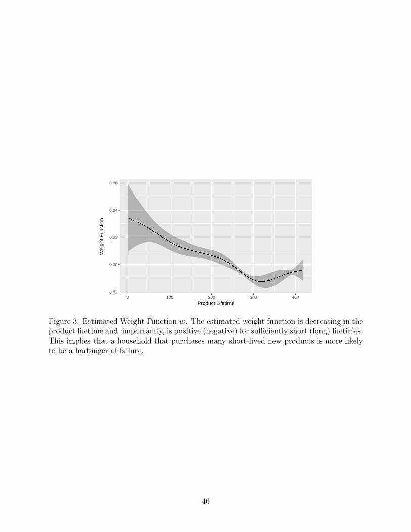
−0.02

0.00

0.02

0.04

0.06

0 100 200 300 400

Product Lifetime

Wei

ght F

unct

ion

Figure 3: Estimated Weight Function w. The estimated weight function is decreasing in theproduct lifetime and, importantly, is positive (negative) for sufficiently short (long) lifetimes.This implies that a household that purchases many short-lived new products is more likelyto be a harbinger of failure.

46

0

20

40

60

−0.01 0.00 0.01 0.02 0.03

βh

Den

sity

Figure 4: Estimates of βh. 44% of households have positive βh thus implying that 44% (56%)of households are harbingers of failure (success).

47

0.4

0.6

0.8

1.0

0 100 200 300

Product Lifetime

Sur

viva

l Pro

babi

lity

Baseline

All success

All failure

Figure 5: Effects of Harbingers on Survival Probability. The solid line provides the Kaplan-Meier estimator of the underlying baseline survival probability. The dashed lines providesaverage survival probability were all sales to harbingers of success and failure. In general,the difference between the survival probability estimates when all sales are to harbingers ofsuccess versus failure is larger than 0.05.

48

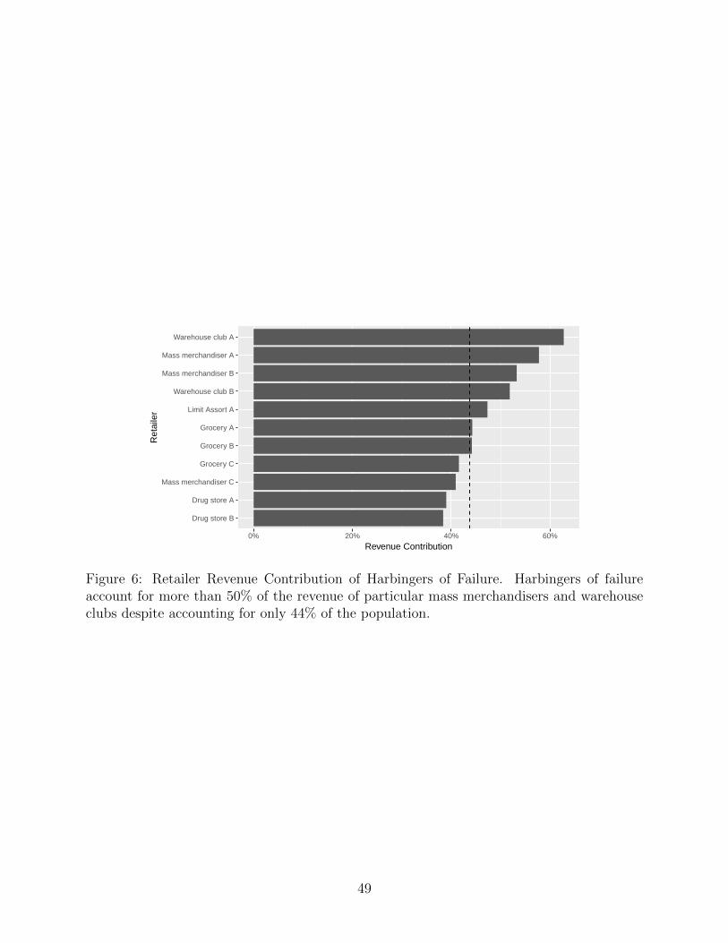
Drug store B

Drug store A

Mass merchandiser C

Grocery C

Grocery B

Grocery A

Limit Assort A

Warehouse club B

Mass merchandiser B

Mass merchandiser A

Warehouse club A

0% 20% 40% 60%

Revenue Contribution

Ret

aile

r

Figure 6: Retailer Revenue Contribution of Harbingers of Failure. Harbingers of failureaccount for more than 50% of the revenue of particular mass merchandisers and warehouseclubs despite accounting for only 44% of the population.

49

Cross−Category

Same Category

0 100 200 300 400

−0.025

0.000

0.025

0.050

−0.025

0.000

0.025

0.050

Product Lifetime

Wei

ght F

unct

ion

Figure 7: Cross-category Estimated Weight Functions w1 and w0. Both weight functions arepositive (negative) for sufficiently short (long) lifetimes. This implies that a household thatpurchases many short-lived new products is more likely to be a harbinger of failure and, asindicated in the bottom panel, this holds even when the product is the calibration datasetis from a different category than the product in the in-sample or out-of-sample dataset.

50

−0.03

−0.02

−0.01

0.00

0 100 200 300 400

Product Lifetime

Wei

ght F

unct

ion

Figure 8: Logistic Regression Estimated Weight Function w. The estimated weight functionis increasing in the product lifetime and, importantly, is negative (postive) for sufficientlyshort (long) lifetimes. This implies that a household that purchases many short-lived newproducts is more likely to be a harbinger of failure.

51

Censored

Uncensored

0 100 200 300 400

−0.04

−0.02

0.00

0.02

0.04

0.06

−0.04

−0.02

0.00

0.02

0.04

0.06

Product Lifetime

Wei

ght F

unct

ion

Figure 9: Estimated Weight Function w in the Full Censoring Model. The top (bottom)panel displays the weight function associated uncensored (censored) new products in thecalibration set. The estimated weight function for uncensored products is positive for shortlifetimes but negative for long lifetimes; this again implies that a household that purchasesmany short-lived new products is more likely to be a harbinger of failure. It also showsthe weight function for censored products is negative which implies that a household thatpurchases new products still being sold is less likely to be a harbinger of failure.

52

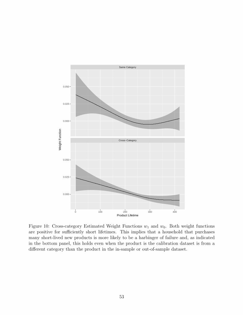
Cross−Category

Same Category

0 100 200 300 400

0.000

0.025

0.050

0.000

0.025

0.050

Product Lifetime

Wei

ght F

unct

ion

Figure 10: Cross-category Estimated Weight Functions w1 and w0. Both weight functionsare positive for sufficiently short lifetimes. This implies that a household that purchasesmany short-lived new products is more likely to be a harbinger of failure and, as indicatedin the bottom panel, this holds even when the product is the calibration dataset is from adifferent category than the product in the in-sample or out-of-sample dataset.

53

Harbingers of Failureand Success - Columbia … approach that yields interpretable consumer-level...

Documents

Transcript of Harbingers of Failureand Success - Columbia … approach that yields interpretable consumer-level...