HAPTER Coping with Bit Errors using Error Correction...

MIT 6.02 DRAFT Lecture Notes

Last update: February 18, 2012

Comments, questions or bug reports?

Please contact hari at mit.edu

CHAPTER 5Coping with Bit Errors using Error

Correction Codes

Recall our main goal in designing digital communication networks: to send informationboth reliably and efficiently between nodes. Meeting that goal requires the use of tech-niques to combat bit errors, which are inevitable in both commmunication channels andstorage media (storage may be viewed as “communication across time”; you store some-thing now and usually want to be able to retrieve it later).

The key idea we will apply to achieve reliable communication is the addition of redun-dancy to the transmitted data, to improve the probability that the original message can bereconstructed from the possibly corrupted data that is received. The sender has an encoderwhose job is to take the message and process it to produce the coded bits that are then sentover the channel. The receiver has a decoder whose job is to take the received (coded) bitsand to produce its best estimate of the message. The encoder-decoder procedures togetherconstitute channel coding; good channel codes provide error correction capabilities thatreduce the bit error rate (i.e., the probability of a bit error).

With proper design, full error correction may be possible, provided only a small num-ber of errors has occurred. Even when too many errors have occurred to permit correction,it may be possible to perform error detection. Error detection provides a way for the re-ceiver to tell (with high probability) if the message was decoded correctly or not. Errordetection usually works by the sender and receiver using a different code from the oneused to correct errors; common examples include the cyclic redundancy check (CRC) or hashfunctions. These codes take n-bit messages and produce a compact “signature” of that mes-sage that is much smaller than the message (e.g., the popular CRC-32 scheme produces a32-bit signature of an arbitrarily long message). The sender computes and transmits thesignature along with the message bits, usually appending it to the end of the message. Thereceiver, after running the decoder to correct errors, then computes the signature over itsestimate of the message bits and compares that signature to its estimate of the signaturebits in the received data. If the computed and estimated signatures are not equal, thenthe receiver considers the message to have one or more bit errors; otherwise, it assumesthat the message has been received correctly. This latter assumption is probabilistic: thereis some non-zero (though very small, for good signatures) probability that the estimated

45

46 CHAPTER 5. COPING WITH BIT ERRORS USING ERROR CORRECTION CODES

and computed signatures match, but the receiver’s decoded message is different from thesender’s. If the signatures don’t match, the receiver and sender may use some higher-layerprotocol to arrange for the message to be retransmitted; we will study such schemes later.We will not study error detection codes like CRC or hash functions in this course.

Our plan for this chapter is as follows. To start, we will assume a binary symmetricchannel (BSC), which we defined and explained in the previous chapter; here the prob-ability of a bit “flipping” is ε. Then, we will discuss and analyze a simple redundancyscheme called a replication code, which will simply make n copies of any given bit. Thereplication code has a code rate of 1/n—that is, for every useful message bit, we end uptransmitting n total bits. The overhead of the replication code of rate c is 1− 1/n, whichis rather high for the error correcting power of the code. We will then turn to the keyideas that allow us to build powerful codes capable of correcting errors without such ahigh overhead (or equivalently, capable of correcting far more errors at a given code ratecompared to the replication code).

There are two big, inter-related ideas used in essentially all error correction codes. Thefirst is the notion of embedding, where the messages one wishes to send are placed in ageometrically pleasing way in a larger space so that the distance between any two validpoints in the embedding is large enough to enable the correction and detection of errors.The second big idea is to use parity calculations, which are linear functions over the bitswe wish to send, to generate the redundancy in the bits that are actually sent. We willstudy examples of embeddings and parity calculations in the context of two classes ofcodes: linear block codes, which are an instance of the broad class of algebraic codes,and convolutional codes, which are perhaps the simplest instance of the broad class ofgraphical codes.

We start with a brief discussion of bit errors.

� 5.1 Bit Errors and BSC

A BSC is characterized by one parameter, ε, which we can assume to be < 1/2, the proba-bility of a bit error. It is a natural discretization of AWGN, which is also a single-parametermodel fully characterized by the variance, σ2. We can determine ε empirically by notingthat if we send N bits over the channel, the expected number of erroneously received bitsis N · ε. By sending a long known bit pattern and counting the fraction or erroneouslyreceived bits, we can estimate ε, thanks to the law of large numbers. In practice, even whenthe BSC is a reasonable error model, the range of ε could be rather large, between 10−2 (oreven a bit higher) all the way to 10−10 or even 10−12. A value of ε of about 10−2 means thatmessages longer than a 100 bits will see at least one error on average; given that the typicalunit of communication over a channel (a “packet”) is generally between 500 bits and 12000bits (or more, in some networks), such an error rate is too high.

But is ε of 10−12 small enough that we don’t need to bother about doing any errorcorrection? The answer often depends on the data rate of the channel. If the channel hasa rate of 10 Gigabits/s (available today even on commodity server-class computers), thenthe “low” ε of 10−12 means that the receiver will see one error every 10 seconds on averageif the channel is continuously loaded. Unless we include some mechanisms to mitigatethe situation, the applications using the channel may find errors occurring too frequently.

SECTION 5.2. THE SIMPLEST CODE: REPLICATION 47

On the other hand, a ε of 10−12 may be fine over a communication channel running at 10Megabits/s, as long as there is some way to detect errors when they occur.

In the BSC model,a transmitted bit b (0 or 1) is interpreted by the receiver as 1− b withprobability ε and as b with probability ε. In this model, each bit is corrupted independentlyand with equal probability (which makes this an “iid” random process, for “independentand identically distributed”). We call ε the bit-flip probability or the “error probability”, andsometimes abuse notation and call it the “bit error rate” (it isn’t really a “rate”, but theterm is still used in the literature). Given a packet of size S bits, it is straightforward tocalculate the probability of the entire packet being received correctly when sent over a BSCwith bit-flip probability ε:

P(packet received correctly) = (1− ε)S.

The packet error probability, i.e., the probability of the packet being incorrect, is 1 minusthis quantity, because a packet is correct if and only if all its bits are correct.

Hence,P(packet error) = 1− (1− ε)S. (5.1)

When ε << 1, a simple first-order approximation of the PER is possible because (1 +x)N ≈ 1 + Nx when |x| << 1. That approximation gives the pleasing result that, whenε << 1,

P(packet error) ≈ 1− (1− Sε) = Sε. (5.2)

The BSC is perhaps the simplest discrete error model that is realistic, but real-worldchannels exhibit more complex behaviors. For example, over many wireless and wiredchannels as well as on storage media (like CDs, DVDs, and disks), errors can occur inbursts. That is, the probability of any given bit being received wrongly depends on recenthistory: the probability is higher if the bits in the recent past were received incorrectly. Ourgoal is to develop techniques to mitigate the effects of both the BSC and burst errors. We’llstart with techniques that work well over a BSC and then discuss how to deal with bursts.

� 5.2 The Simplest Code: Replication

In general, a channel code provides a way to map message words to codewords (analogousto a source code, except here the purpose is not compression but rather the addition ofredundancy for error correction or detection). In a replication code, each bit b is encodedas n copies of b, and the result is delivered. If we consider bit b to be the message word,then the corresponding codeword is bn (i.e., bb...b, n times). In this example, there are onlytwo possible message words (0 and 1) and two corresponding codewords. The replicationcode is absurdly simple, yet it’s instructive and sometimes even useful in practice!

But how well does it correct errors? To answer this question, we will write out theprobability of overcoming channel errors for the BSC error model with the replication code.That is, if the channel corrupts each bit with probability ε, what is the probability that thereceiver decodes the received codeword correctly to produce the message word that wassent?

The answer depends on the decoding method used. A reasonable decoding method ismaximum likelihood decoding: given a received codeword, r, which is some n-bit combina-


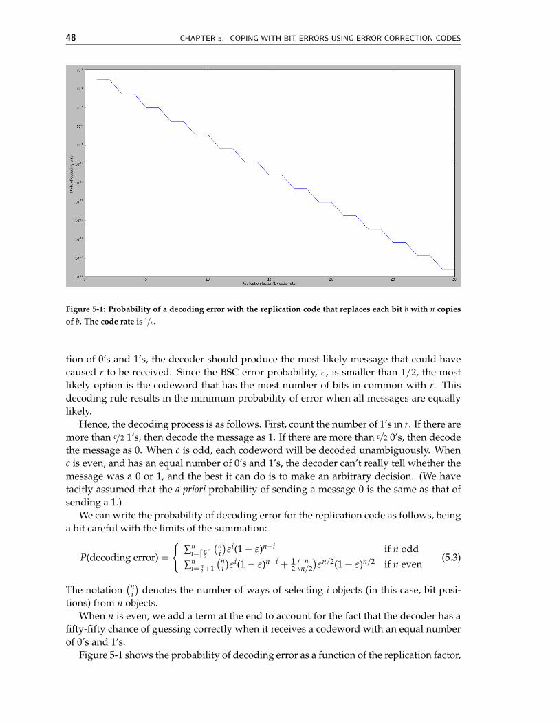
Figure 5-1: Probability of a decoding error with the replication code that replaces each bit b with n copiesof b. The code rate is 1/n.

tion of 0’s and 1’s, the decoder should produce the most likely message that could havecaused r to be received. Since the BSC error probability, ε, is smaller than 1/2, the mostlikely option is the codeword that has the most number of bits in common with r. Thisdecoding rule results in the minimum probability of error when all messages are equallylikely.

Hence, the decoding process is as follows. First, count the number of 1’s in r. If there aremore than c/2 1’s, then decode the message as 1. If there are more than c/2 0’s, then decodethe message as 0. When c is odd, each codeword will be decoded unambiguously. Whenc is even, and has an equal number of 0’s and 1’s, the decoder can’t really tell whether themessage was a 0 or 1, and the best it can do is to make an arbitrary decision. (We havetacitly assumed that the a priori probability of sending a message 0 is the same as that ofsending a 1.)

We can write the probability of decoding error for the replication code as follows, beinga bit careful with the limits of the summation:

P(decoding error) =

�∑n

i=� n2 �

�ni�εi(1− ε)n−i if n odd

∑ni= n

2 +1�n

i�εi(1− ε)n−i + 1

2� n

n/2�εn/2(1− ε)n/2 if n even

(5.3)

The notation�n

i�

denotes the number of ways of selecting i objects (in this case, bit posi-tions) from n objects.

When n is even, we add a term at the end to account for the fact that the decoder has afifty-fifty chance of guessing correctly when it receives a codeword with an equal numberof 0’s and 1’s.

Figure 5-1 shows the probability of decoding error as a function of the replication factor,

SECTION 5.3. EMBEDDINGS AND HAMMING DISTANCE 49

n, for the replication code, computed using Equation (5.3). The y-axis is on a log scale, andthe probability of error is more or less a straight line with negative slope (if you ignorethe flat pieces), which means that the decoding error probability decreases exponentiallywith the code rate. It is also worth noting that the error probability is the same whenn = 2� as when n = 2�− 1. The reason, of course, is that the decoder obtains no additionalinformation that it already didn’t know from any 2�− 1 of the received bits.

Despite the exponential reduction in the probability of decoding error as n increases,the replication code is extremely inefficient in terms of the overhead it incurs, for a givenrate, 1/n. As such, it is used only in situations when bandwidth is plentiful and there isn’tmuch computation time to implement a more complex decoder.

We now turn to developing more sophisticated codes. There are two big related ideas:embedding messages into spaces in a way that achieves structural separation and parity (linear)computations over the message bits.

� 5.3 Embeddings and Hamming Distance

Let’s start our investigation into error correction by examining the situations in whicherror detection and correction are possible. For simplicity, we will focus on single-errorcorrection (SEC) here. By that we mean codes that are guaranteed to produce the correctmessage word, given a received codeword with zero or one bit errors in it. If the receivedcodeword has more than one bit error, then we can make no guarantees (the method mightreturn the correct message word, but there is at least one instance where it will return thewrong answer).

There are 2n possible n-bit strings. Define the Hamming distance (HD) between two n-bit words, w1 and w2, as the number of bit positions in which the messages differ. Thus0 ≤ HD(w1, w2) ≤ n.

Suppose that HD(w1, w2) = 1. Consider what happens if we transmit w1 and there’sa single bit error that inconveniently occurs at the one bit position in which w1 and w2differ. From the receiver’s point of view it just received w2—the receiver can’t detect thedifference between receiving w1 with a unfortunately placed bit error and receiving w2.In this case, we cannot guarantee that all single bit errors will be corrected if we choose acode where w1 and w2 are both valid codewords.

What happens if we increase the Hamming distance between any two valid codewordsto 2? More formally, let’s restrict ourselves to only sending some subset S = {w1, w2, ..., ws}of the 2n possible words such that

HD(wi, wj) ≥ 2 for all wi, wj ∈ S where i �= j (5.4)

Thus if the transmission of wi is corrupted by a single error, the result is not an elementof S and hence can be detected as an erroneous reception by the receiver, which knowswhich messages are elements of S. A simple example is shown in Figure 5-2: 00 and 11 arevalid codewords, and the receptions 01 and 10 are surely erroneous.

We define the minimum Hamming distance of a code as the minimum Hamming distancebetween any two codewords in the code. From the discussion above, it should be easy tosee what happens if we use a code whose minimum Hamming distance is D. We state theproperty formally:


Figure 5-2: Codewords separated by a Hamming distance of 2 can be used to detect single bit errors. Thecodewords are shaded in each picture. The picture on the left is a (2,1) repetition code, which maps 1-bitmessages to 2-bit codewords. The code on the right is a (3,2) code, which maps 2-bit messages to 3-bitcodewords.

Theorem 5.1 A code with a minimum Hamming distance of D can detect any error pattern ofD− 1 or fewer errors. Moreover, there is at least one error pattern with D errors that cannot bedetected reliably.

Hence, if our goal is to detect errors, we can use an embedding of the set of messages wewish to transmit into a bigger space, so that the minimum Hamming distance between anytwo codewords in the bigger space is at least one more than the number of errors we wishto detect. (We will discuss how to produce such embeddings in the subsequent sections.)

But what about the problem of correcting errors? Let’s go back to Figure 5-2, with S ={00,11}. Suppose the received sequence is 01. The receiver can tell that a single error hasoccurred, but it can’t tell whether the correct data sent was 00 or 11—both those possiblepatterns are equally likely under the BSC error model.

Ah, but we can extend our approach by producing an embedding with more spacebetween valid codewords! Suppose we limit our selection of messages in S even further,as follows:

HD(wi, wj) ≥ 3 for all wi, wj ∈ S where i �= j (5.5)

How does it help to increase the minimum Hamming distance to 3? Let’s define onemore piece of notation: let Ewi be the set of messages resulting from corrupting wi with asingle error. For example, E000 = {001,010,100}. Note that HD(wi,an element of Ewi ) = 1.

With a minimum Hamming distance of 3 between the valid codewords, observe thatthere is no intersection between Ewi and Ewj when i �= j. Why is that? Suppose therewas a message wk that was in both Ewi and Ewj . We know that HD(wi, wk) = 1 andHD(wj, wk) = 1, which implies that wi and wj differ in at most two bits and consequentlyHD(wi, wj) ≤ 2. (This result is an application of Theorem 5.2 below, which states that theHamming distance satisfies the triangle inequality.) That contradicts our specification thattheir minimum Hamming distance be 3. So the Ewi don’t intersect.

So now we can correct single bit errors as well: the received message is either a memberof S (no errors), or is a member of some particular Ewi (one error), in which case the receivercan deduce the original message was wi. Here’s another simple example: let S = {000,111}.

SECTION 5.3. EMBEDDINGS AND HAMMING DISTANCE 51

So E000 = {001,010,100} and E111 = {110,101,011} (note that E000 doesn’t intersect E111).Suppose the received sequence is 101. The receiver can tell there has been a single errorbecause 101 /∈ S. Moreover it can deduce that the original message was most likely 111because 101 ∈ E111.

We can formally state some properties from the above discussion, and specify the error-correcting power of a code whose minimum Hamming distance is D.

Theorem 5.2 The Hamming distance between n-bit words satisfies the triangle inequality. Thatis, HD(x, y) + HD(y, z) ≥ HD(x, z).

Theorem 5.3 For a BSC error model with bit error probability < 1/2, the maximum likelihood de-coding strategy is to map any received word to the valid codeword with smallest Hamming distancefrom the received one (ties may be broken arbitrarily).

Theorem 5.4 A code with a minimum Hamming distance of D can correct any error pattern of�D−1

2 � or fewer errors. Moreover, there is at least one error pattern with �D−12 �+ 1 errors that

cannot be corrected reliably.

Equation (5.5) gives us a way of determining if single-bit error correction can alwaysbe performed on a proposed set S of transmission messages—we could write a programto compute the Hamming distance between all pairs of messages in S and verify that theminimum Hamming distance was at least 3. We can also easily generalize this idea tocheck if a code can always correct more errors. And we can use the observations madeabove to decode any received word: just find the closest valid codeword to the receivedone, and then use the known mapping between each distinct message and the codewordto produce the message. The message will be the correct one if the actual number of errorsis no larger than the number for which error correction is guaranteed. The check for thenearest codeword may be exponential in the number of message bits we would like tosend, making it a reasonable approach only if the number of bits is small.

But how do we go about finding a good embedding (i.e., good code words)? This taskisn’t straightforward, as the following example shows. Suppose we want to reliably send4-bit messages so that the receiver can correct all single-bit errors in the received words.Clearly, we need to find a set of messages S with 24 elements. What should the membersof S be?

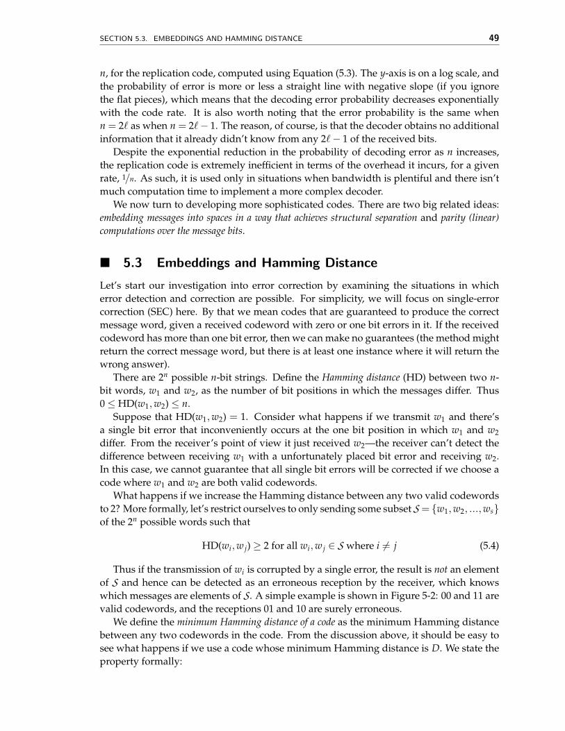
The answer isn’t obvious. Once again, we could write a program to search throughpossible sets of n-bit messages until it finds a set of size 16 with a minimum Hammingdistance of 3. An exhaustive search shows that the minimum n is 7, and one example of Sis:

0000000 1100001 1100110 00001110101010 1001011 1001100 01011011010010 0110011 0110100 10101011111000 0011001 0011110 1111111

But such exhaustive searches are impractical when we want to send even modestlylonger messages. So we’d like some constructive technique for building S. Much of thetheory and practice of coding is devoted to finding such constructions and developingefficient encoding and decoding strategies.


Broadly speaking, there are two classes of code constructions, each with an enormousnumber of example instances. The first is the class of algebraic block codes. The secondis the class of graphical codes. We will study two simple examples of linear block codes,which themselves are a sub-class of algebraic block codes: rectangular parity codes andHamming codes. We also note that the replication code discussed in Section 5.2 is anexample of a linear block code.

In the next two chapters, we will study convolutional codes, a sub-class of graphicalcodes.

� 5.4 Linear Block Codes and Parity Calculations

Linear block codes are examples of algebraic block codes, which take the set of k-bit mes-sages we wish to send (there are 2k of them) and produce a set of 2k codewords, each n bitslong (n ≥ k) using algebraic operations over the block. The word “block” refers to the factthat any long bit stream can be broken up into k-bit blocks, which are each then expandedto produce n-bit codewords that are sent.

Such codes are also called (n, k) codes, where k message bits are combined to producen code bits (so each codeword has n− k “redundancy” bits). Often, we use the notation(n, k, d), where d refers to the minimum Hamming distance of the block code. The rate of ablock code is defined as k/n; the larger the rate, the less the redundancy overhead incurredby the code.

A linear code (whether a block code or not) produces codewords from message bits byrestricting the algebraic operations to linear functions over the message bits. By linear, wemean that any given bit in a valid codeword is computed as the weighted sum of one ormore original message bits.

Linear codes, as we will see, are both powerful and efficient to implement. They arewidely used in practice. In fact, all the codes we will study—including convolutionalcodes—are linear, as are most of the codes widely used in practice. We already lookedat the properties of a simple linear block code: the replication code we discussed in Sec-tion 5.2 is a linear block code with parameters (n,1, n).

An important and popular class of linear codes are binary linear codes. The computationsin the case of a binary code use arithmetic modulo 2, which has a special name: algebrain a Galois Field of order 2, also denoted F2. A field must define rules for addition andmultiplication, and their inverses. Addition in F2 is according to the following rules: 0 +0 = 1 + 1 = 0; 1 + 0 = 0 + 1 = 1. Multiplication is as usual: 0 · 0 = 0 · 1 = 1 · 0 = 0; 1 · 1 = 1.We leave you to figure out the additive and multiplicative inverses of 0 and 1. Our focusin this book will be on linear codes over F2, but there are natural generalizations to fieldsof higher order (in particular, Reed Solomon codes, which are over Galois Fields of order2q).

A linear code is characterized by the following theorem, which is both a necessary anda sufficient condition for a code to be linear:

Theorem 5.5 A code is linear if, and only if, the sum of any two codewords is another codeword.

For example, the block code defined by codewords 000,101,011 is not a linear code,because 101 + 011 = 110 is not a codeword. But if we add 110 to the set, we get a lin-

SECTION 5.5. RECTANGULAR PARITY SEC CODE 53

ear code because the sum of any two codewords is now another codeword. The code000,101,011,110 has a minimum Hamming distance of 2 (that is, the smallest Hammingdistance between any two codewords in 2), and can be used to detect all single-bit errorsthat occur during the transmission of a code word. You can also verify that the minimumHamming distance of this code is equal to the smallest number of 1’s in a non-zero code-word. In fact, that’s a general property of all linear block codes, which we state formallybelow:

Theorem 5.6 Define the weight of a codeword as the number of 1’s in the word. Then, the mini-mum Hamming distance of a linear block code is equal to the weight of the non-zero codeword withthe smallest weight.

To see why, use the property that the sum of any two codewords must also be a code-word, and that the Hamming distance between any two codewords is equal to the weightof their sum (i.e., weight(u + v) = HD(u, v)). (In fact, the Hamming distance between anytwo bit-strings of equal length is equal to the weight of their sum.) We leave the completeproof of this theorem as a useful and instructive exercise for the reader.

The rest of this section shows how to construct linear block codes over F2. For simplicity,and without much loss of generality, we will focus on correcting single-bit errors. i.e.,on single-error correction (SEC) codes.. We will show two ways of building the set S oftransmission messages to have single-error correction capability, and will describe howthe receiver can perform error correction on the (possibly corrupted) received messages.

We will start with the rectangular parity code in Section 5.5, and then discuss the clevererand more efficient Hamming code in Section 5.7.

� 5.5 Rectangular Parity SEC Code

We define the parity of bits x1, x2, . . . , xn as (x1 + x2 + . . . + xn), where the addition is per-formed modulo 2 (it’s the same as taking the exclusive OR of the n bits). The parity is evenwhen the sum is 0 (i.e., the number of ones is even), and odd otherwise.

Let parity(s) denote the parity of all the bits in the bit-string s. We’ll use a dot, ·, toindicate the concatenation (sequential joining) of two messages or a message and a bit. Forany message M (a sequence of one or more bits), let w = M · parity(M). You should beable to confirm that parity(w) = 0. This code, which adds a parity bit to each message,is also called the even parity code, because the number of ones in each codeword is even.Even parity lets us detect single errors because the set of codewords, {w}, each defined asM · parity(M), has a Hamming distance of 2.

If we transmit w when we want to send some message M, then the receiver can take thereceived word, r, and compute parity(r) to determine if a single error has occurred. Thereceiver’s parity calculation returns 1 if an odd number of the bits in the received messagehas been corrupted. When the receiver’s parity calculation returns a 1, we say there hasbeen a parity error.

This section describes a simple approach to building an SEC code by constructing mul-tiple parity bits, each over various subsets of the message bits, and then using the resultingparity errors (or non-errors) to help pinpoint which bit was corrupted.


d11 d12 d13 d14 p row(1)d21 d22 d23 d24 p row(2)

p col(1) p col(2) p col(3) p col(4)

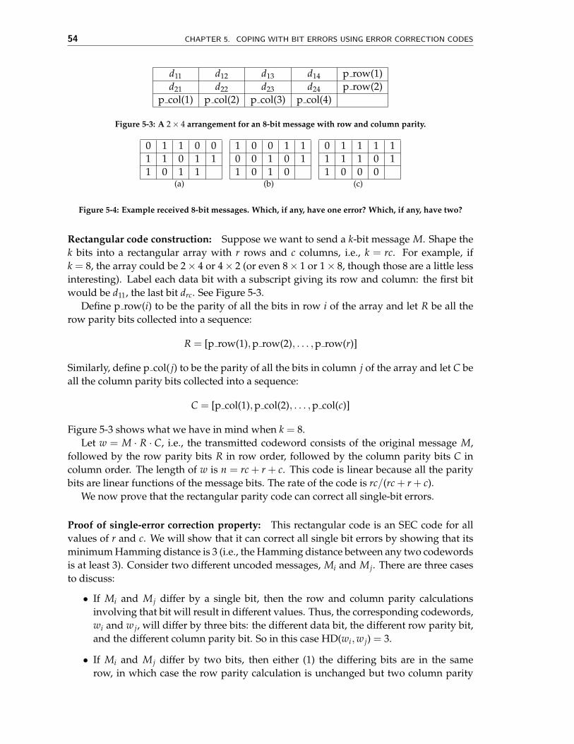
Figure 5-3: A 2× 4 arrangement for an 8-bit message with row and column parity.

0 1 1 0 01 1 0 1 11 0 1 1

(a)

1 0 0 1 10 0 1 0 11 0 1 0

(b)

0 1 1 1 11 1 1 0 11 0 0 0

(c)

Figure 5-4: Example received 8-bit messages. Which, if any, have one error? Which, if any, have two?

Rectangular code construction: Suppose we want to send a k-bit message M. Shape thek bits into a rectangular array with r rows and c columns, i.e., k = rc. For example, ifk = 8, the array could be 2× 4 or 4× 2 (or even 8× 1 or 1× 8, though those are a little lessinteresting). Label each data bit with a subscript giving its row and column: the first bitwould be d11, the last bit drc. See Figure 5-3.

Define p row(i) to be the parity of all the bits in row i of the array and let R be all therow parity bits collected into a sequence:

R = [p row(1),p row(2), . . . ,p row(r)]

Similarly, define p col( j) to be the parity of all the bits in column j of the array and let C beall the column parity bits collected into a sequence:

C = [p col(1),p col(2), . . . ,p col(c)]

Figure 5-3 shows what we have in mind when k = 8.Let w = M · R · C, i.e., the transmitted codeword consists of the original message M,

followed by the row parity bits R in row order, followed by the column parity bits C incolumn order. The length of w is n = rc + r + c. This code is linear because all the paritybits are linear functions of the message bits. The rate of the code is rc/(rc + r + c).

We now prove that the rectangular parity code can correct all single-bit errors.

Proof of single-error correction property: This rectangular code is an SEC code for allvalues of r and c. We will show that it can correct all single bit errors by showing that itsminimum Hamming distance is 3 (i.e., the Hamming distance between any two codewordsis at least 3). Consider two different uncoded messages, Mi and Mj. There are three casesto discuss:

• If Mi and Mj differ by a single bit, then the row and column parity calculationsinvolving that bit will result in different values. Thus, the corresponding codewords,wi and wj, will differ by three bits: the different data bit, the different row parity bit,and the different column parity bit. So in this case HD(wi, wj) = 3.

• If Mi and Mj differ by two bits, then either (1) the differing bits are in the samerow, in which case the row parity calculation is unchanged but two column parity

SECTION 5.5. RECTANGULAR PARITY SEC CODE 55

calculations will differ, (2) the differing bits are in the same column, in which case thecolumn parity calculation is unchanged but two row parity calculations will differ,or (3) the differing bits are in different rows and columns, in which case there will betwo row and two column parity calculations that differ. So in this case HD(wi, wj) ≥4.

• If Mi and Mj differ by three or more bits, then HD(wi, wj) ≥ 3 because wi and wjcontain Mi and Mj respectively.

Hence we can conclude that HD(wi, wj) ≥ 3 and our simple “rectangular” code will beable to correct all single-bit errors.

Decoding the rectangular code: How can the receiver’s decoder correctly deduce Mfrom the received w, which may or may not have a single bit error? (If w has more thanone error, then the decoder does not have to produce a correct answer.)

Upon receiving a possibly corrupted w, the receiver checks the parity for the rows andcolumns by computing the sum of the appropriate data bits and the corresponding paritybit (all arithmetic in F2). This sum will be 1 if there is a parity error. Then:

• If there are no parity errors, then there has not been a single error, so the receiver canuse the data bits as-is for M. This situation is shown in Figure 5-4(a).

• If there is single row or column parity error, then the corresponding parity bit is inerror. But the data bits are okay and can be used as-is for M. This situation is shownin Figure 5-4(c), which has a parity error only in the fourth column.

• If there is one row and one column parity error, then the data bit in that row andcolumn has an error. The decoder repairs the error by flipping that data bit and thenuses the repaired data bits for M. This situation is shown in Figure 5-4(b), wherethere are parity errors in the first row and fourth column indicating that d14 shouldbe flipped to be a 0.

• Other combinations of row and column parity errors indicate that multiple errorshave occurred. There’s no “right” action the receiver can undertake because itdoesn’t have sufficient information to determine which bits are in error. A commonapproach is to use the data bits as-is for M. If they happen to be in error, that will bedetected by the error detection code (mentioned near the beginning of this chapter).

This recipe will produce the most likely message, M, from the received codeword if therehas been at most a single transmission error.

In the rectangular code the number of parity bits grows at least as fast as√

k (it shouldbe easy to verify that the smallest number of parity bits occurs when the number of rows,r, and the number of columns, c, are equal). Given a fixed amount of communication“bandwidth” or resource, we’re interested in devoting as much of it as possible to sendingmessage bits, not parity bits. Are there other SEC codes that have better code rates thanour simple rectangular code? A natural question to ask is: how little redundancy can we getaway with and still manage to correct errors?

The Hamming code uses a clever construction that uses the intuition developed whileanswering the question mentioned above. We answer this question next.


Figure 5-5: A codeword in systematic form for a block code. Any linear code can be transformed into anequivalent systematic code.

� 5.6 How many parity bits are needed in an SEC code?

Let’s think about what we’re trying to accomplish with an SEC code: the correction oftransmissions that have a single error. For a transmitted message of length n there aren + 1 situations the receiver has to distinguish between: no errors and a single error ina specified position along the string of n received bits. Then, depending on the detectedsituation, the receiver can make, if necessary, the appropriate correction.

Our first observation, which we will state here without proof, is that any linear codecan be transformed into an equivalent systematic code. A systematic code is one whereevery n-bit codeword can be represented as the original k-bit message followed by then− k parity bits (it actually doesn’t matter how the original message bits and parity bitsare interspersed). Figure 5-5 shows a codeword in systematic form.

So, given a systematic code, how many parity bits do we absolutely need? We needto choose n so that single error correction is possible. Since there are n − k parity bits,each combination of these bits must represent some error condition that we must be ableto correct (or infer that there were no errors). There are 2n−k possible distinct parity bitcombinations, which means that we can distinguish at most that many error conditions.We therefore arrive at the constraint

n + 1 ≤ 2n−k (5.6)

i.e., there have to be enough parity bits to distinguish all corrective actions that mightneed to be taken (including no action). Given k, we can determine n− k, the number ofparity bits needed to satisfy this constraint. Taking the log (to base 2) of both sides, wecan see that the number of parity bits must grow at least logarithmically with the numberof message bits. Not all codes achieve this minimum (e.g., the rectangular code doesn’t),but the Hamming code, which we describe next, does.

We also note that the reasoning here for an SEC code can be extended to determine alower bound on the number of parity bits needed to correct t > 1 errors.

� 5.7 Hamming Codes

Intuitively, it makes sense that for a code to be efficient, each parity bit should protectas many data bits as possible. By symmetry, we’d expect each parity bit to do the sameamount of “work” in the sense that each parity bit would protect the same number of data

SECTION 5.7. HAMMING CODES 57

d1 p1 p2

p3

d2 d3

d4

(a) (7,4) code

d1 p1 p2

p3

d2 d3

d4

p4

d9

d11

d10

d6

d7 d5

d8

(b) (15,11) code

Figure 5-6: Venn diagrams of Hamming codes showing which data bits are protected by each parity bit.

bits. If some parity bit is shirking its duties, it’s likely we’ll need a larger number of paritybits in order to ensure that each possible single error will produce a unique combinationof parity errors (it’s the unique combinations that the receiver uses to deduce which bit, ifany, had an error).

The class of Hamming single error correcting codes is noteworthy because they areparticularly efficient in the use of parity bits: the number of parity bits used by Hammingcodes grows logarithmically with the size of the codeword. Figure 5-6 shows two examplesof the class: the (7,4) and (15,11) Hamming codes. The (7,4) Hamming code uses 3 paritybits to protect 4 data bits; 3 of the 4 data bits are involved in each parity computation. The(15,11) Hamming code uses 4 parity bits to protect 11 data bits, and 7 of the 11 data bits areused in each parity computation (these properties will become apparent when we discussthe logic behind the construction of the Hamming code in Section 5.7.1).

Looking at the diagrams, which show the data bits involved in each parity computation,you should convince yourself that each possible single error (don’t forget errors in one ofthe parity bits!) results in a unique combination of parity errors. Let’s work through theargument for the (7,4) Hamming code. Here are the parity-check computations performedby the receiver:

E1 = (d1 + d2 + d4 + p1) mod 2E2 = (d1 + d3 + d4 + p2) mod 2E3 = (d2 + d3 + d4 + p3) mod 2

where each Ei is called a syndrome bit because it helps the receiver diagnose the “illness”(errors) in the received data. For each combination of syndrome bits, we can look forthe bits in each codeword that appear in all the Ei computations that produced 1; thesebits are potential candidates for having an error since any of them could have caused theobserved parity errors. Now eliminate from the candidates those bits that appear in any Eicomputations that produced 0 since those calculations prove those bits didn’t have errors.


We’ll be left with either no bits (no errors occurred) or one bit (the bit with the single error).For example, if E1 = 1, E2 = 0 and E3 = 1, we notice that bits d2 and d4 both appear

in the computations for E1 and E3. However, d4 appears in the computation for E2 andshould be eliminated, leaving d2 as the sole candidate as the bit with the error.

Another example: suppose E1 = 1, E2 = 0 and E3 = 0. Any of the bits appearing in thecomputation for E1 could have caused the observed parity error. Eliminating those thatappear in the computations for E2 and E3, we’re left with p1, which must be the bit withthe error.

Applying this reasoning to each possible combination of parity errors, we can make atable that shows the appropriate corrective action for each combination of the syndromebits:

E3E2E1 Corrective Action000 no errors001 p1 has an error, flip to correct010 p2 has an error, flip to correct011 d1 has an error, flip to correct100 p3 has an error, flip to correct101 d2 has an error, flip to correct110 d3 has an error, flip to correct111 d4 has an error, flip to correct

� 5.7.1 Is There a Logic to the Hamming Code Construction?

So far so good, but the allocation of data bits to parity-bit computations may seem ratherarbitrary and it’s not clear how to build the corrective action table except by inspection.

The cleverness of Hamming codes is revealed if we order the data and parity bits in acertain way and assign each bit an index, starting with 1:

index 1 2 3 4 5 6 7binary index 001 010 011 100 101 110 111

(7,4) code p1 p2 d1 p3 d2 d3 d4

This table was constructed by first allocating the parity bits to indices that are powersof two (e.g., 1, 2, 4, . . . ). Then the data bits are allocated to the so-far unassigned indicies,starting with the smallest index. It’s easy to see how to extend this construction to anynumber of data bits, remembering to add additional parity bits at indices that are a powerof two.

Allocating the data bits to parity computations is accomplished by looking at their re-spective indices in the table above. Note that we’re talking about the index in the table, notthe subscript of the bit. Specifically, di is included in the computation of pj if (and only if)the logical AND of binary index(di) and binary index(pj) is non-zero. Put another way, diis included in the computation of pj if, and only if, index(pj) contributes to index(di) whenwriting the latter as sums of powers of 2.

So the computation of p1 (with an index of 1) includes all data bits with odd indices: d1,d2 and d4. And the computation of p2 (with an index of 2) includes d1, d3 and d4. Finally,the computation of p3 (with an index of 4) includes d2, d3 and d4. You should verify thatthese calculations match the Ei equations given above.


If the parity/syndrome computations are constructed this way, it turns out that E3E2E1,treated as a binary number, gives the index of the bit that should be corrected. For exam-ple, if E3E2E1 = 101, then we should correct the message bit with index 5, i.e., d2. Thiscorrective action is exactly the one described in the earlier table we built by inspection.

The Hamming code’s syndrome calculation and subsequent corrective action can be ef-ficiently implemented using digital logic and so these codes are widely used in contextswhere single error correction needs to be fast, e.g., correction of memory errors when fetch-ing data from DRAM.

� Acknowledgments

Many thanks to Katrina LaCurts for carefully reading these notes and making several use-ful comments.


� Problems and Questions

1. Prove that the Hamming distance satisfies the triangle inequality. That is, show thatHD(x, y) + HD(y, z) ≥ HD(x, z) for any three n-bit binary words.

2. Consider the following rectangular linear block code:

D0 D1 D2 D3 D4 | P0D5 D6 D7 D8 D9 | P1D10 D11 D12 D13 D14 | P2-------------------------P3 P4 P5 P6 P7 |

Here, D0–D14 are data bits, P0–P2 are row parity bits and P3–P7 are column paritybits. What are n, k, and d for this linear code?

3. Consider a rectangular parity code as described in Section 5.5. Ben Bitdiddle wouldlike use this code at a variety of different code rates and experiment with them onsome channel.

(a) Is it possible to obtain a rate lower than 1/3 with this code? Explain your an-swer.

(b) Suppose he is interested in code rates like 1/2, 2/3, 3/4, etc.; i.e., in general arate of �−1

l , for some integer � > 1. Is it always possible to pick the parameters ofthe code (i.e, the block size and the number of rows and columns over which toconstruct the parity bits) so that any such code rate of the form �−1

l is achievable?Explain your answer.

4. Two-Bit Communications (TBC), a slightly suspect network provider, uses the fol-lowing linear block code over its channels. All arithmetic is in F2.

P0 = D0, P1 = (D0 + D1), P2 = D1.

(a) What are n and k for this code?(b) Suppose we want to perform syndrome decoding over the received bits. Write

out the three syndrome equations for E0, E1, E2.(c) For the eight possible syndrome values, determine what error can be detected

(none, error in a particular data or parity bit, or multiple errors). Make yourchoice using maximum likelihood decoding, assuming a small bit error prob-ability (i.e., the smallest number of errors that’s consistent with the given syn-drome).

(d) Suppose that the the 5-bit blocks arrive at the receiver in the following order:D0, D1, P0, P1, P2. If 11011 arrives, what will the TBC receiver report as the re-ceived data after error correction has been performed? Explain your answer.

(e) TBC would like to improve the code rate while still maintaining single-bit errorcorrection. Their engineer would like to reduce the number of parity bits by 1.Give the formulas for P0 and P1 that will accomplish this goal, or briefly explainwhy no such code is possible.


5. Pairwise Communications has developed a linear block code over F2 with three dataand three parity bits, which it calls the pairwise code:

P1 = D1 + D2 (Each Di is a data bit; each Pi is a parity bit.)P2 = D2 + D3

P3 = D3 + D1

(a) Fill in the values of the following three attributes of this code:(i) Code rate =(ii) Number of 1s in a minimum-weight non-zero codeword =(iii) Minimum Hamming distance of the code =

6. Consider the same “pairwise code” as in the previous problem. The receiver com-putes three syndrome bits from the (possibly corrupted) received data and paritybits: E1 = D1 + D2 + P1, E2 = D2 + D3 + P2, and E3 = D3 + D1 + P3. The receiverperforms maximum likelihood decoding using the syndrome bits. For the combi-nations of syndrome bits in the table below, state what the maximum-likelihood de-coder believes has occured: no errors, a single error in a specific bit (state which one),or multiple errors.

E3E2E1 Error pattern [No errors / Error in bit ... (specify bit) / Multiple errors]0 0 00 0 10 1 00 1 11 0 01 0 11 1 01 1 1

7. Alyssa P. Hacker extends the aforementioned pairwise code by adding an overall par-ity bit. That is, she computes P4 = ∑3

i=1(Di + Pi), and appends P4 to each original code-word to produce the new set of codewords. What improvement in error correctionor detection capabilities, if any, does Alyssa’s extended code show over Pairwise’soriginal code? Explain your answer.

8. For each of the sets of codewords below, determine whether the code is a linear blockcode over F2 or not. Also give the rate of each code.

(a) {000,001,010,011}.

(b) {000, 011, 110, 101}.

(c) {111, 100, 001, 010}.

(d) {00000, 01111, 10100, 11011}.

(e) {00000}.


9. For any linear block code over F2 with minimum Hamming distance at least 2t + 1between codewords, show that:

2n−k ≥ 1 +�

n1

�+

�n2

�+ . . .

�nt

�.

Hint: How many errors can such a code always correct?

10. For each (n, k, d) combination below, state whether a linear block code with thoseparameters exists or not. Please provide a brief explanation for each case: if such acode exists, give an example; if not, you may rely on a suitable necessary condition.

(a) (31,26,3): Yes / No

(b) (32,27,3): Yes / No

(c) (43,42,2): Yes / No

(d) (27,18,3): Yes / No

(e) (11,5,5): Yes / No

11. Using the Hamming code construction for the (7,4) code, construct the parity equa-tions for the (15,11) code. How many equations does this code have? How manymessage bits contribute to each parity bit?

12. Prove Theorems 5.2 and 5.3. (Don’t worry too much if you can’t prove the latter; wewill give the proof when we discuss convolutional codes in Lecture 8.)

13. The weight of a codeword in a linear block code over F2 is the number of 1’s inthe word. Show that any linear block code must either: (1) have only even weightcodewords, or (2) have an equal number of even and odd weight codewords.Hint: Proof by contradiction.

14. There are N people in a room, each wearing a hat colored red or blue, standing in aline in order of increasing height. Each person can see only the hats of the people infront, and does not know the color of his or her own hat. They play a game as a team,whose rules are simple. Each person gets to say one word: “red” or “blue”. If theword they say correctly guesses the color of their hat, the team gets 1 point; if theyguess wrong, 0 points. Before the game begins, they can get together to agree on aprotocol (i.e., what word they will say under what conditions). Once they determinethe protocol, they stop talking, form the line, and are given their hats at random.

Can you develop a protocol that will maximize their score? What score does yourprotocol achieve?

HAPTER Coping with Bit Errors using Error Correction...

Documents

Transcript of HAPTER Coping with Bit Errors using Error Correction...