Hankerson-WIMC2005

8/3/2019 Hankerson-WIMC2005

http://slidepdf.com/reader/full/hankerson-wimc2005 1/110

Implementing Elliptic Curve Cryptography (a narrow survey)

Institute of Computing – UNICAMP

Campinas, Brazil April 2005

Darrel HankersonAuburn University

Implementing ECC – 1/110



Overview

Objective: sample selected topics of practical interest.

Talk will favor:

Software solutions on general-purpose processors

rather than dedicated hardware.

Techniques with broad applicability.

Methods targeted to standardized curves.

Goals:

Present proposed methods in context.

Limit coverage of technical details (but “implementing”necessarily involves platform considerations).




Focus: higher-performance processors

“Higher-performance” includes processors commonlyassociated with workstations, but also found in surprisingly

small portable devices.

Sun and IBM workstations RIM pager circa 1999

SPARC or Intel x86 (Pentium) Intel x86 (custom 386)

256 MB – 8 GB 2 MB “disk”, 304 KB RAM

0.5 GHz – 3 GHz 10 MHz, single AA battery

heats entire building fits in shirt pocket




Optimizing ECC

Elliptic Curve Digital Signature

Algorithm (ECDSA)

Big number and

arithmetic

Random number

modular arithmetic

Curve

arithmetic

qF field

generation

General categories of optimization efforts:

1. Field-level optimizations.

2. Curve-level optimizations.

3. Protocol-level optimizations.

Constraints: security requirements, hardware limitations,

bandwidth, interoperability, and patents.




Optimizing ECC...

1. Field-level optimizations. Choose fields with fast multiplication and inversion.

Use special-purpose hardware (cryptographic

coprocessors, DSP, floating-point, SIMD).

2. Curve-level optimizations.

Reduce the number of point additions (windowing).

Reduce the number of field inversions (projective

coords). Replace point doubles (endomorphism methods).

3. Protocol-level optimizations.

Develop efficient protocols. Choose methods and protocols that favor your

computations or hardware.




Context: Protocols such as ECDSA

The Elliptic Curve Digital Signature Algorithm (ECDSA) isthe elliptic curve analogue of the DSA.

Provides data origin authentication, data integrity, and

non-repudiation.

Jan 1999 ECDSA formally approved as an ANSI standard –

ANSI X9.62.

Jan 2000 ECDSA formally approved as a US Federal Gov stan-dard – FIPS 186-2.

Aug 2000 ECDSA formally approved as an IEEE standard –

IEEE 1363-2000

Feb 2005 NSA recommends algs for securing US Gov sensitive

but unclassified data: ECDSA selected for authenti-

cation.




ECDSA Signature Generation

Signer A has domain parameters D (consisting of the curve,field, base point G, etc.), private key d , and public key

Q = dG. B has authentic copies of D and Q.

To sign a message m, A does the following:1. Select a random integer k from [1, n − 1].

2. Compute kG = ( x1, y1) and r = x1 mod n.

3. Compute e = SHA-1(m).4. Compute s = k −1{e + dr } mod n.

5. A’s signature for the message m is (r , s).

The computationally expensive operation is the scalarmultiplication

kG = G + G + · · ·+ G

k times

in step 2, for a point G which is known a priori.Implementing ECC – 7/110



ECDSA Verification

To verify A’s signature (r , s) on m, B does:1. Verify that r and s are integers in [1, n − 1].

2. Compute e = SHA-1(m).

3. Compute w = s−1

mod n.4. Compute u1 = ew mod n and u2 = rw mod n.

5. Compute u1G + u2Q = ( x1, y1).

6. Compute v = x1 mod n.7. Accept the signature if and only if v = r .

The computationally expensive operation is the scalar

multiplications u1G and u2Q in step 5, where only G is

known a priori.




Deployment Notes...

US National Security Agency (NSA) and ECC

Fall 2003

NSA obtains licensing rights to Menezes-Qu-Vanstone

(MQV). Covers curves over F p for 256-bit or larger p.

February 2005, at the RSA conference

NSA presents strategy and recommendations for

securing US Gov sensitive and unclassified

communications.

“Suite B” protocols for key agreement and

authentication are ECC only: ECMQV and ECDH forkey agreement, and ECDSA for auth.




Deployment Notes...

Example: BlackBerry 2-way pager

Marketing demands 256-bit AES.

Key size comparison.

Symmetric cipher

key length

Example

algorithm

ECC key

length

RSA/DL key

length80 SKIPJACK 160 1024

112 Triple-DES 224 2048

128 AES-Small 256 3072

192 AES-Medium 384 8192256 AES-Large 512 15360

ECC especially attractive here.




Deployment Notes...

Timings on BlackBerry 7230 for 128-bit security.

ECC (256) RSA (3072) DH (3072)

Key generation 166 ms Too long 38 s

Encrypt or verify 150 ms 52 ms 74 sDecript or sign 168 ms 8 s 74 s

Source: Herb Little, RIM.

BlackBerry EC algorithms.Facility Protocol

Over the Air (OTA) Provisioning ECSPEKEa (ECDH-512)

Policy Authentication ECDSAOTA Re-key ECMQV

aSimple Password Exponential Key Exhange.

RSA-1024 used for code signing (for verify speed).




Topic I

Prerequisites




Elliptic curve groups

1. Interested in elliptic curves in simplified Weierstrass

forms

y2 = x3 + ax + b, char K = 2, 3

y

2

+ xy = x

3

+ ax

2

+ b, char K = 2.over finite fields K .

2. E (K ) = {( x, y) ∈ K ×K | ( x, y) solves the equation}∪{∞}.

3. The chord-and-tangent rule make E (K ) into an abeliangroup with the point at infinity ∞ as the identity.

4. Scalar (or point) multiplication is the operation

kP = P + P + · · · + P k times

where k is an integer.




Chord-and-tangent rule

R = ( x3, y3)

x

y

P = ( x1, y1)

Q = ( x2, y2)

(a) Addition: P + Q = R.

R = ( x3, y3)

x

y

P = ( x1, y1)

(b) Doubling: P + P = R.

Geometric addition and doubling of elliptic curve points




Point Arithmetic

R = ( x3, y3)

x

y

P = ( x1, y1)

Q = ( x2, y2)

R = ( x3, y3)

x

y

P = ( x1, y1)

Addition and Doubling

Let P = ( x1, y1), Q = ( x2, y2).

op λ x y

char K /∈ {2, 3}, curve: y2 = x3 + ax + b−P x1 − y1

P + Q ( y2− y1)/( x2− x1) λ 2 − x1 − x2 λ ( x1 − x) − y1

2P (3 x21 + a)/2 y1 λ 2

−2 x1 λ ( x1

− x)

− y1

char K = 2, curve: y2 + xy = x3 + ax2 + b

−P x1 x1 + y1

P + Q ( y1+ y2)/( x1+ x2) λ 2 +λ + x1 + x2 + a λ ( x1 + x) + x + y1

2P x1 + y1/ x1 λ 2 +λ + a = x21 + b x2

1 x21 +λ x + x




Calculating kP

Simple double-and-add approach:

1. Write k =t −1

∑i=0

k i2i for k i ∈ {0, 1}.

2. Q←∞.

3. For i from t − 1 to 0 do3.1 Q←2Q.

3.2 If k i = 1 then Q←Q + P.

4. Return Q.

Analysis: t point doubles and expected t /2 additions.

Improving the performance:

Reduce the number of point additions (windowing). Reduce the number of field inversions (projective

coordinates).

Replace point doubles (efficient endomorphisms).

Use curves over fields where fast arithmetic is available.Implementing ECC – 16/110



Calculating kP...

Simple double-and-add approach has t point doublings and

an expected t /2 additions.

Reduce adds by writing k in non-adjacent form (NAF):

NAF(k ) =

t

∑i=0

k i2i, where k i ∈ {0,±1} and k i+ik i = 0.

1. Find NAF(k ) =t

∑i=0

k i2i. Set Q

←∞.

2. For i from t to 0 do

2.1 Q←2Q.

2.2 If k i = 1 then Q←Q + P.

2.3 If k i = −1 then Q←Q − P.3. Return Q.

Analysis: t point doublings and an expected t /3 additions.




Width- w NAF

NAF reduces the number of required point additions. Can be

generalized to a width- w NAF .

1. k =t

∑i=0

k i2i, where k i ∈ {0,±1,±3,. .. ,±2w−1 − 1}.

2. Among w consecutive digits, at most one is nonzero.

3. t ≤ log2 k + 1.

4. Density is 1/(w + 1). A NAF is a width-2 NAF.

Example: 13 (base 10) has expansions

(1, 0,

−1, 0, 1) NAF

= (1, 1, 0, 1) binary

= 1310 = 1

·24 + (

−3)

·20 = (1, 0, 0, 0,

−3) width-3 NAF

.

Analysis: kP by width-w NAF has t doublings and an ex-

pected t /(w + 1) additions.




Width- w NAF...

Calculting the w-NAF is inexpensive.

Solinas [DCC 2000] gives alg using only simple bit

operations.

Digits of w-NAF k = ∑k i2i produced right-to-left (k 0first).

Some point mult algs want to process left-to-right, so

typically digits of w-NAF are stored.

Avanzi [SAC 2004] gives (optimal) left-to-right calculation of

w-NAF variant. See also Muir and Stinson [CACR Tech

Rep].


M ’ h d



Montgomery’s method

Montgomery’s method is a useful benchmark for point

multiplication algorithms for curves

y2 + xy = x3 + ax2 + b

over binary fields. (Due to López and Dahab and based on

an idea of Montgomery.)

Let Q1 = ( x1, y1) and Q2 = ( x2, y2) with Q1 = ±Q2.

Let Q1 + Q2 = ( x3, y3) and Q1 − Q2 = ( x4, y4). Then

x3 = x4 +x2

x1 + x2

+x2

x1 + x22

.

Thus, the x-coordinate of Q1 + Q2 can be computed

from the x-coordinates of Q1, Q2 and Q1 − Q2.


M t ’ th d



Montgomery’s method...

(k t −1k t −2 · · ·k t − j k t −( j+1) k t −( j+2) · · ·k 1k 0)2P

↓ ↓

[lP, (l + 1)P] → [2lP, lP + (l + 1)P], if k t −( j+1) = 0[lP + (l + 1)P, 2(l + 1)P], if k t −( j+1) = 1

Each iteration requires one doubling and one addition. Possesses natural resistance to some side-channel

attacks.

No extra storage. Produces only the x-coordinate of the result, sufficient

for ECDSA.


Obt i i th di t



Obtaining the y-coordinate

Two methods to find y-coordinate from a Montgomery

multiplication:

1. (Direct) After the last iteration, have the x-coordinates

of kP = ( x1, y1) and (k + 1)P = ( x2, y2). y-coordinate of

kP can be recovered as: y1 = x−1( x1 + x)[( x1 + x)( x2 + x) + x2 + y] + y.

(Derived using the addition formula for x-coord x2 of

(k + 1)P from kP = ( x1, y1) and P = ( x, y).)

2. (Point compression method) Guess at the y-coordinate

of kP (e.g., solve quadratic y2 + x1 y = x21 + ax2

1 + b),

obtaining ˜ y1.Compute the x-coord of ( x1, ˜ y1) + ( x, y). If this agrees

with the x-coord of (k + 1)P then set y1 = ˜ y1; otherwise

set y1 = ˜ y1 + x1.Implementing ECC – 22/110

Projective coordinates




Let c, d be positive integers. Define equivalence relation∼on K 3\{(0, 0, 0)} by

( X 1,Y 1, Z 1) ∼ ( X 2,Y 2, Z 2) if ( X 1,Y 1, Z 1) = (λ c X 2,λ d Y 2,λ Z 2)

for some λ ∈

K ∗. An equivalence class is called a projective

point .

Projective form Relation Name

Curve: y2 = x3 + ax + b

Y 2 Z = X 3 + aX Z 2 + bZ 3 ( X / Z ,Y / Z ) projective

Y 2 = X 3 + aX Z 4 + bZ 6 ( X / Z 2,Y / Z 3) Jacobian

Curve: y2 + xy = x3 + ax2 + b

Y 2 Z + XYZ = X 3 + aX 2 Z + bZ 3 ( X / Z ,Y / Z ) projective

Y 2 + XYZ = X 3 + aX 2 Z 2 + bZ 6 ( X / Z 2,Y / Z 3) Jacobian

Y 2 + XYZ = X 3 Z + aX 2 Z 2 + bZ 4 ( X / Z ,Y / Z 2) López-Dahab (LD)





Projective coordinates...

Field inversion is typically expensive relative to field

multiplication.

Projective coordinates reduce the number of field

inversions in point arithmetic.

Point addition in affine for F2m :

λ ←( y1+ y2)/( x1+ x2)

x←λ 2

+λ + x1 + x2 + a, y←λ ( x1 + x) + x + y1

Projective ( X : Y : Z ) = ( X 1 : Y 1 : Z 1) + ( X 2 : Y 2 : 1):

A

←Y 2 Z 21 +Y 1, B

← X 2 Z 1 + X 1, C

← Z 1 B, D

← B2(C + aZ 21 ),

Z ←C 2, E ← AC , X ← A2 + D + E , F ← X + X 2 Z ,

G←( X 2 +Y 2) Z 2, Y ←( E + Z )F + G.





Projective coordinates...

Affine vs projective field operation counts:

Doubling Addition (mixed)

Curve y2 + xy = x3 + ax2 + b, a ∈ {0, 1}Affine 1 I , 2 M 1 I , 2 M

López-Dahab ( X / Z ,Y / Z 2) 4 M 8 M Curve y2 = x3 + ax + b, a = −3

Affine 1 I , 2 M , 2S 1 I , 2 M , 1S

Jacobian ( X / Z 2,Y / Z 3) 4 M , 4S 8 M , 3S

I = inversion, M = multiplication, S = squaring

Rough estimate of threshold I / M in binary case: kP by

non-adjacent form I + 2 M +

1

3( I + 2 M ) = D +

1

3 A

affine

≤ Dproj +1

3 Aproj = 4 M +

1

38 M

projective

gives I ≤ 3 M .Implementing ECC – 25/110



Appendix: NIST curves over binary fields



Appendix: NIST curves over binary fields

1. Koblitz curves:

K-163 y2 + xy = x3 + x2 + 1 over F2163 , cofactor 2

f = x163 + x7 + x6 + x3 + 1

K-233 y2 + xy = x3 + 1 over F2

233 , cofactor 4

f = x233 + x74 + 1

K-283 y2 + xy = x3 + 1 over F2283 , cofactor 4

f = x283 + x12 + x7 + x5 + 1

K-409 y2

+ xy = x3

+ 1 over F2409 , cofactor 4 f = x409 + x87 + 1

K-571 y2 + xy = x3 + 1 over F2571 , cofactor 4

f = x571 + x10 + x5 + x2 + 1

2. Randomly-generated curves B-{163, 233, 283, 409,

571} over each of these fields, each with cofactor 2:

y

2

+ xy = x

3

+ x

2

+ b.Implementing ECC – 27/110

Appendix: NIST curves over prime fields



Appendix: NIST curves over prime fields

Curves y2

=x3

− 3 x

+b randomly generated and have

prime order.

Curve Prime p

P-192 2192 − 264 − 1

P-224 2224 − 296 + 1

P-256 2256

−2224 + 2192 + 296

−1

P-384 2384 − 2128 − 296 + 232 − 1

P-521 2521 − 1

Special form of the prime speeds reduction.


Appendix: Basic facts for curves over prime fields



Appendix: Basic facts for curves over prime fields

1. There are about 2 p different elliptic curves over F p.

2. E (F p) is an abelian group with identity ∞.

3. (Hasse’s Theorem ) The number of points on the elliptic

curve is # E (F p) = p + 1−

t where|t | ≤

2√

p; that is,

p + 1 − 2√ p ≤ # E (F p) ≤ p + 1 + 2√ p.

Hence, # E (F p) ≈ p.

4. # E (F p) can be computed in polynomial time usingSchoof’s algorithm .

5. E (F p) is isomorphic to Zn1⊕Zn2

where n2 divides both

n1 and p − 1.

Corresponding facts hold if F p is replaced by any finite field.




Topic II

Endomorphism methods


Reducing the cost of doubling



Reducing the cost of doubling

1. Use projective coordinates when I / M is large.

Eliminates most field inversions.

2. Use precomputation if the point is known in advance

(e.g., in signature generation) and the additionalmemory requirement is acceptable.

3. Replace doubling by halving in the binary case.

4. Replace (some) doublings by other efficiently

computable maps.


Replace doublings: efficient endomorphisms



p b g p

1. (multiplication by m map) [m] : P→

mP. Special case:

P → −P.

2. (qth power map) φ : ( x, y) → ( xq, yq) for E defined over

Fq. Particular case: Koblitz curves, q = 2.

3. Let p ≡ 1 (mod 3). Consider E : y2 = x3 + b defined

over F p. If β ∈ F p is of order 3, then

φ :( x

, y

) → (β x

, y

)is an endomorphism.

For q = 2, the map in 2 is inexpensive compared with field

mult, and the map in 3 is a single field mult.

Koblitz curves: inexpensive applications of φ replace point

doubles. (Point halving has similar goal.)

Example 3 allows the number of doublings to be reduced.Implementing ECC – 32/110

Koblitz curves



Define curves over F2:

E 0 : y2 + xy = x3 + 1

E 1 : y2 + xy = x3 + x2 + 1

am−1

Ò Ò Õ Õ Õ Õ Õ

· · · a1

( ( W W W

W Wa0

7 7 u u u u u u u

am−1 0 · · · 0 a1 0 a0

Squaring a binary polynomial

am−1 zm−1

+ . . .+ a1 z + a0.

(Frobenius map) τ : ( x, y) → ( x2, y2).

τ 2P + 2P = µτ (P) for µ = (−1)1−a and curve points P.

τ 2 + 2 = µτ =⇒ τ = µ+√−72

.

Makes sense to multiply points in E a(F2m) by elements

of Z[τ ]:

(ulτ l + · · · + u1τ + u0)P = ulτ

l(P) + · · · + u1τ (P) + u0P

Applying τ (field squaring) is inexpensive in comparison to

field multiplication.Implementing ECC – 33/110

Strategy for kP on a Koblitz curve



gy

Basic idea: since field squaring is cheap, expand k as ∑k iτ i

with |k i| small and sparse (to reduce the number of required

point additions).

Z

[τ ] is Euclidean with respect to N : α → αα . Finding a width-w τ -NAF is analogous to ordinary

width-w NAF: for odd r 0 + r 1τ , the element of the

equivalence class (mod τ w) is subtracted, and the

result is divisible by τ w.

Example: representatives are α u = u mod τ w. If w = 3and a = 0, then α 1 = 1, α 3 = τ + 1, and

5 = −τ 5 + 0τ 4 + 0τ 3 + 0τ 2 + 0τ 1 − (τ + 1)τ 0

gives a width-3 τ -NAF of 5. Then 5P = −τ 5α 1P −α 3P.


Strategy...



gy

To compute kP for P in the main subgroup of E (F2m):

1. Compute α uP for odd u < 2w−1.

2. Compute k = k mod (τ m − 1)/(τ −1) in Z[τ ].

3. Find the width-w τ -adic expansion ∑t i=0 ciτ

i of k ,where t ≈ m and ci ∈ {±α u}∪{0}.

4. Q←∞.

5. For i from t to 0 do

5.1 Q←τ Q.

5.2 If ci = 0 then add or subtract appropriate α uP.

6. Return (Q).

No point doublings. Expect roughly m/(w + 1) point

additions.

J. Solinas, Efficient arithmetic on Koblitz curves. Designs, Codes

and Cryptography, 2000.


Operation counts



Point doubles and additions expected in finding kP for a

curve over F2m with m = 233.

curve method doubles adds

random double and add 232 116

NAF 232 78

width-4 NAF 1+232 3+47

Koblitz τ -NAF 0 78

width-4 τ -NAF 0 3+47

Applying τ requires two or three field squarings, each

costing roughly 15% of a field multiplication. Finding k (for the τ -adic NAF) is not free.


Using efficient endomorphisms



GLV observed that an endomorphism may be used to

reduce the number of doubles (even if a Koblitz-likeexpansion is not efficient).

Example (WAP)

Let p ≡ 1 (mod 3). (In P-160, p = 2160 − 229233.)

Let E : y2 = x3 + b, and let β ∈ F p be an element of

order 3.

φ : ( x, y) → (β x, y) is an endomorphism.

Computing φ requires only 1 field multiplication.

|φ

|= 1.

1. Gallant, Lambert, and Vanstone. Faster point multiplication on

elliptic curves with efficient endomorphisms, CRYPTO 2001.

2. Park, Jeong, and Kim. An alternate decomposition of an integerfor faster point multiplication on certain elliptic curves, PKC 2002.


Using efficient endomorphisms...



Let G

∈ E (F p) be a point of prime order n.

φ acts on G by multiplication: φ P = λ P, where λ is a

root (modulo n) of the characteristic polynomial of φ .

(λ 2 +λ

≡ −1 (mod n) in the example.)

To compute kP:

• Write k ≡ k 1 + k 2λ (mod n) where |k i| ≈√

n. (This

can be done efficiently.)

• kP = k 1P + k 2λ P = k 1P + k 2φ (P), which can be

computed via interleaving.

k 1,t · · · k 1,1 k 1,0 width-w NAF of k 1k 2,t · · · k 2,1 k 2,0 width-w NAF of k 2

Approx half the doubles are eliminated. Cost of finding

k i negligible if domain parameters are set in advance.


A very special case



Solinas (CORR 2001-41) gives an example where finding k 1and k 2 is free.

p = 2390 + 3

≡1 (mod 3)

E : y2 = x3 − 2 over F p

n = # E (F p) = 2390 − 2195 + 7 = 63r , r prime

λ =2195

−2

3 , β = 2389

+ 2194

+ 1 mod p =⇒ λ ( x, y) = (β x, y)

Write k = k 22195 + k 1 for k 1 < 2195. Then

kP= (

2195k 2 +

k 1)

P= ((

3λ +

2)

k 2 +

k 1)

P= (

2k 2 +

k 1)

k 1

P+

3k 2

k 2

λ P

= k 1( x, y) + k 2((2389 + 2194 + 1) x, y)

The cost of calculating β x is less than a field multiplication.Implementing ECC – 39/110

Point halving for curves over binary fields



Doubling in affine: seek 2P = ( x2, y2) from P = ( x, y).

Let λ = x + y/ x. Calculate:

x2 = x2 + b/ x2

y2 = x2 +λ x2 + x2

(2 mul, 1 mul by b, 1 inv)

or

x2 = λ 2 +λ + a

y2 = x2 +λ x2 + x2

(2 mul, 1 inv)

Halving: seek P = ( x, y) from 2P = ( x2, y2). Basic idea:

solve x2 = λ 2 +λ + a for λ

y2 = x2 +λ x2 + x2 for x

1. E. Knudsen, Elliptic scalar multiplication using point halving,

Asiacrypt ’99.

2. R. Schroeppel, Elliptic curve point ambiguity resolution apparatus

and method, patent application, 2000.


Point halving...



Facts

1. Tr(c) = c + c2 + · · · + c2m−1 ∈ {0, 1}.

2. The NIST random binary curves all have Tr(a) = 1.

Tr( x(kG)) = Tr(a) for generator G.

Halving for the trace 1 case

1. Solve

λ 2 + λ = x2 + a

obtaining λ = λ or λ = λ + 1.

2. Since y2 = x2 +λ x2 + x2, consider

x2 = ( λ + 1) x2 + y2

Tr( x2) = Tr( x) = Tr(a) = 1, so Tr((

λ + 1) x2 + y2)

identifies λ .

3. Find x = x2(λ + 1) + y2.Implementing ECC – 41/110

Point halving...



Halving: ( x2, y2)→

( x,λ = x + y/ x) where 2( x, y) = ( x2, y2);

y may be recovered via

λ x = x2 + y =⇒ y = λ x + x2 (≈ 1 field mult)

Algorithm (point halving) INPUT: ( x2,λ 2) or ( x2, y2).

OUTPUT: ( x,λ = x + y/ x) where 2( x, y) = ( x2, y2).

Steps Cost

1. Solve λ 2 + λ = x2 + a for λ . ≈

2/3 field mult

2. Find T = x2( λ +λ 2 + x2 + 1) ≈ 1 field mult

or T = x2(

λ + 1) + y2

3. If Tr(T ) = 1 then λ = λ , x =√

T Tr

≈free

else λ = λ + 1, x = √T + x2. root ≈ 1/2 field mult

4. Return( x,λ ).

Conversion to affine ( x,λ )

→( x, y) is

≈1 field mult.

(Doubling in projective ≈ 4 field mults.)Implementing ECC – 42/110

Calculating kP by halve-and-add



Algorithm (halve-and-add, right-to-left)

INPUT: point P and scalar k . OUTPUT: kP.

1. (Precomputation) Solve quadratic equations (21–30 field el-

ements for B -163). Build table of 16 multiples of√

x.

2. (Transform k ) Solvek = k t 2

t + · · · + k 0 = k t /2t + · · · + k 1/2 + k 0 (mod n)

for k ; i.e., 2t k mod n = k 02t + · · · + k t .

3. Q

←∞.

4. For i from 0 to t do4.1 If k i = 1 then Q←Q + P.

4.2 P←P/2.

5. Return(Q).

Looks best when I / M small.

Multiple accumulators allow right-to-left with width-w

NAF variant.Implementing ECC – 43/110

Summary: Efficient endomorphisms



1. If curve can be selected, GLV offers a dramatic

speedup for on-line precomp case.

2. Halving is a significant improvement for kP on binary

curves in on-line precomp case, especially if I / M is

small.

3. Frobenius endomorphism τ on Koblitz curves is

significantly better than halving.

4. Siet, Lange, Sica, Quisquater [SAC 2002] extend

Koblitz-like expansions to other curves. Less useful if

the endomorphism costs more than 1/2 point double.


Summary: Efficient endomorphisms...



5. Avanzi, Siet, and Sica [PKC 2004] give a scalar

recoding that combines a halving step with Frobeniusmethod on Koblitz curves. Trades some point additions

for a halving.

Practical interest may be limited, since it seemsunlikely that there’s room for halving code, but not

for an additional point of storage and 3-TNAF.




Appendix: Timings (800 MHz Intel Pentium III)



NIST Field Pentium III (800 MHz)

curve Method mult M normalized M µs

Unknown point ( kP, on-line precomputation)

P-192 5-NAF (w = 5) 2016 2016 975

B-163 4-NAF (w = 4) 954 2953 1475

B-163 Halving (w = 4) 687 2126 1050K-163 5-TNAF (w = 5) 365 1130 625

Fixed base ( kP, off-line precomputation)

P-192 Comb 2-table (w = 4) 718 718 325

B-163 Comb 386 1195 575K-163 6-TNAF (w = 6) 263 814 475

Multiple point multiplication ( kP + lQ )

P-192 Interleave (w = 6, 5) 2306 2306 1150

B-163 Interleave (w = 6, 4) 1154 3572 1800

K-163 Interleave TNAF (w = 6, 5) 565 1749 1000

Timings using general-purpose registers. M is the estimated field multiplicationswith I / M = 80 and I / M = 8 in the prime and binary fields. Normalization gives

equivalent P-192 field mults for this implementation.


Appendix: Timings...



1. Timings for Koblitz curves significantly faster than for

random binary or prime in on-line precomp case.

2. Faster prime field multiplication gives P-192 the edge

for off-line precomp case.

3. Results depend on processor and implementation. Only general-purpose registers used.

Pentium III has floating-point registers which can accelerate

prime field arithmetic, and single-instruction multiple-data(SIMD) registers that are easily harnessed for binary fields.

Integer multiplication with general-purpose registers on P-III

is faster than on earlier or newer Pentium family processors.

P-192 may be less competitive if hardware mult is weaker oroperates on fewer bits.

4. The case where a large amount of storage is available

for precomp in known-point methods is not addressed.Implementing ECC – 48/110



Topic III

Normal Basis Arithmetic


Normal bases in characteristic 2



Representing F2m field elements:

Polynomial basis: {1, x, . . . , xm−1}, reduction poly f .

Normal basis: {β 20,β 2

1,β 2

2, . . . ,β 2

m−1}.

Motivation for use of normal basis reps:

Squaring, square root are shifts. x2 + x = c can be

solved bitwise.

Performance of square root and quadratic solver isfundamental to methods based on point halving.

Low complexity (Gaussian) NB bases have especiallynice arithmetic.

Methods in 1990s seem to confirm that NB mult will be very

slow in software compared to PB.

Ning & Yin [ICICS 2001] precompute shifts and significantly

improve NB mult (at the cost of data-dependent storage).Implementing ECC – 50/110

NB Multiplication



Obtain the multplication table for basis

{β 2

i

}:

β 2i

β 2 j

=m−1

∑s=0

λ (s)i j β 2

s

,

Then c = ab is given by

cs =m−1

∑i=0

m−1

∑ j=0

ai+sb j+sλ (0)i j .

Define m×m matrix M = [λ (0)i j ]:

cs = (asas+1 . . . as+m−1) M (bsbs+1 . . . bs+m−1).

Number of 1s in M is the complexity C M . C M ≥ 2m − 1. Basis is optimal if C M = 2m − 1.

Optimal bases introduced by Mullin, Onyszchuk,

Vanstone, and Wilson to reduce hardware complexity.Implementing ECC – 51/110

Gaussian normal bases



Optimal bases are relatively rare. Only m = 233 in the NIST

recommended fields has an ONB.

Generalization: Gaussian normal bases.

Let p = mT + 1 be a prime. K = u where u ∈Z

∗ p hasorder T .

Suppose index e of 2 in Z∗ p satisfies gcd(e, m) = 1.

Then

Z∗ p = {2iu j | 0 ≤ i < m, 0 ≤ j < T },

and K i = K 2i for 0 ≤ i < m are the cosets of K in Z∗ p.

p | 2mT

− 1 =⇒ there is a primitive pth root of unityα ∈ F2mT .

Gauss periods of type (m, T ) are β i = ∑ j∈K iα j for

0

≤i < m.


Gaussian normal bases...



Let β = β 0. Then β i = β 2i

, and

{β 2

i

}is a normal basis

for F2m called a type T GNB .

C M ≤ mT − 1. T is a measure of the complexity of themult.

ONBs are precisely the GNBs with T ∈ {1, 2}.

NIST recommended fields F2m and type of GNB.

m 163 233 283 409 571

Type 4 2 6 4 10


Vector multiplication



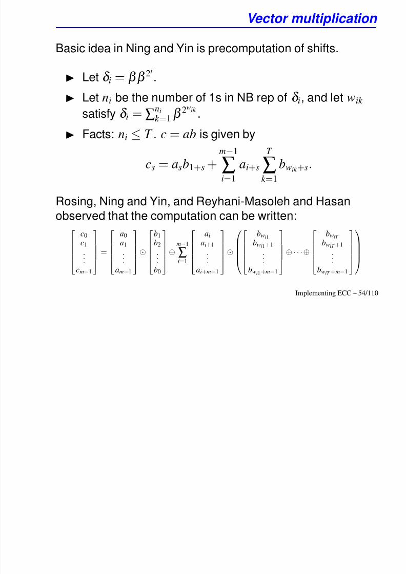
Basic idea in Ning and Yin is precomputation of shifts.

Let δ i = ββ 2i

.

Let ni be the number of 1s in NB rep of δ i, and let wik

satisfy δ i = ∑ni

k =1β 2wik

.

Facts: ni ≤ T . c = ab is given by

cs = asb1+s +

m−1

∑i=1 ai+s

T

∑k =1 bwik +s.

Rosing, Ning and Yin, and Reyhani-Masoleh and Hasan

observed that the computation can be written:

c0

c1

.

.

.

cm

−1

=

a0

a1

.

.

.

am

−1

b1

b2

.

.

.

b0

⊕m−1

∑i=1

ai

ai+1

.

.

.

ai+m

−1

bwi1

bwi1+1

.

.

.

bwi1 +m

−1

⊕· · ·⊕

bwiT

bwiT +1

.

.

.

bwiT +m

−1


Vector multiplication...



To find c = ab:

Precompute all m required shifts for a and b.

Copy the precomputation to simplify indexing in

evaluation phase. Total storage: 4m words.

Evaluation has mT XOR and m AND operations on field

elements.

Variations (Dahab, H, Hu, Long, López, Menezes):

Efficient one-table (e.g., precomputation for a only)

versions.

For type 1, use matrix decompostion of Hasan, Wang,and Bhargava to reduce complexity to essentially m.

(But type 1 means m is even.)


Vector multiplication...



The good news

Significantly faster than preceding methods in software

for NB.

Easy to code and relatively easy to optimize.

Some bad news

2m or 4m words of dynamic storage.

Still much slower than methods for polynomial basis.

F2m field multiplication (in µs), 800 MHz Intel Pentium III. Other

than L-D, input and output are in NB.

L-D Ning&Yin DHHLLM

m Type comb 2 table 1 table Ring map

162 1 1.3 6.7 5.0∗ 2.7

163 4 1.3 9.6 8.4 10.4

233 2 2.3 11.4 11.7 7.1

∗Uses matrix decomposition.Implementing ECC – 56/110

Ring mapping method



Basic idea for GNB: map to an associated ring and use fast

methods for polynomial basis reps.

Basis conversion approach

Technique is well-known for the type 1 case, where the

mapping is a permutation.

Sunar and Koç [ToC 2001] is a basis conversion

approach for type 2 that exploits properties of the map.

Ring mapping approach

Arithmetic in the ring is modulo a cyclotomic polynomial

(and so has especially simple reduction).

“Palindromic representation” of Blake, Roth, andSeroussi is the special case for type 2.

General case has a factor T expansion, a significant

hurdle.Implementing ECC – 57/110

Ring mapping method...



Assume β is a Gauss period of type (m, T ) and is a normal

element. For a ∈ F2m :

a =m−1

∑i=0

aiβ 2i

=m−1

∑i=0

ai ∑ j

∈K i

α j =mT

∑ j=1

a jα

j

where a j = ai if j ∈ K i.

Let R = F2[ x]/(Φ p) where Φ p( x) = ( x p

−1)/( x

−1).

φ :m−1

∑i=0

aiβ 2i →

mT

∑ j=1

a j x

j

is a ring homomorphism from F2m to R, and

φ (F2m) = {c1 x + · · · + cmT xmT ∈| c j = ck for j, k ∈ K i}.

φ and its inverse are relatively inexpensive, and

arithmetic in R benefits from form of Φ p.Implementing ECC – 58/110

Ring mapping method...

N ï h i h i d h l i f



Naïve approach: map into the ring and then exploit fast

polynomial-based arithmetic.

There is a factor T expansion, which can be significant.

For F2163 , T is at least 4.

If T is even (always the case if m is odd), then the last

mT /2 coefficients for elements in φ (F2m ) are a mirror

reflection of the first mT /2 [WHBG].

Symmetry property is well-known in the case T = 2where Gauss periods produce a type 2 optimal normal

basis of the form

{(α +α −1

)2i

| 0 ≤ i < m}and there is an associated basis

{α i +α 2m+1−i | 1 ≤ i ≤ m}.


Gauss periods and mapping for small parameters

C id F f 3 T 4 i i T + 1 13



Consider F2m for m = 3. T = 4 gives prime p = mT + 1 = 13

and the unique subgroup of order T = 4 in Z∗13 isK = {1,−1, 5,−5}. The mapping into

R = F2[ x]/(Φ p) for Φ p( x) = ( x13

−1)/( x

−1)

is given by

φ : a = (a0, a1, a2) → (a0, a1, a1, a2, a0, a2, a2, a0, a2, a1, a1, a0).

φ (a) is symmetric about p/2 and hence the first( p − 1)/2 coeffs of the ring element suffice to invert φ .

Fewer coefficients may suffice: in the example, the first

4 (rather than ( p−

1)/2 = 6) coeffs will allow recovery

of the field element.

Wu, Hasan, Blake and Gao [ToC 2002] give sample

minima for the number of consecutive R-element coeffs

that permits recovery of the associated field element.Implementing ECC – 60/110

Algorithm: Multiplication via ring mapping

1 2i 1 2i



INPUT: elements a = ∑m−1i=

0 aiβ 2i

and b = ∑m−1i=

0 biβ 2i

in F2m .

OUTPUT: c = ab = ∑m−1i=0 ciβ

2i

.

1. Calculate

a = φ (a) = p−

1

∑ j=1

a j x

j

in R where a j = ai if j

∈K i. Do similarly for b.

2. Apply a fast multiplication method for polynomial-based

reps to find half the coeffs of c = ab in R.

3. Returnc = φ −

1

(c).


Observations on the ring mapping algorithm

1 φ can be optimized with per field precomp Each output



1. φ can be optimized with per-field precomp. Each output

coefficient is obtained with a word shift and mask.Only the first half are calculated in this fashion;

remainder obtained by symmetry.

2. The López-Dahab “comb” method provides fastmultiplication for polynomials and can be adapted to

find only some of the output coefficients.

3. Reduction via

Φ p( x) =x p − 1

x − 1= x p−1 + x p−2 + · · · + x + 1

is fast.

4. Only half the output coefficients are required.

5. Cost of applying φ is approximately T /2 times the cost

of φ −1.


Example: ring mapping method for m = 163

F 163 has a type T 4 normal basis and hence the mapping



F2163 has a type T = 4 normal basis, and hence the mapping

gives a factor 4 expansion.

Modified comb mult finds mT /2 = 326 coeffs of the

product ab. With 32-bit words, field elements require 6

words and ring elements require 21. Comb finds words 0,. .. , 10, 19,. .. , 30 of the complete

42-word polynomial product.

Small optimization: word 10 is not required since fieldelt can be recovered from c1,. .. , c

309 of product c.

The cost of an application of φ is approx 10% of the

total field mult time (φ −

1 costs approx half of φ ).

Experimentally, times on an Intel Pentium III are a factor 7

slower than field mult for a polynomial basis rep.

Competitive with the best methods with a NB rep.Implementing ECC – 63/110

Example: ring mapping method for m = 233

F 233 has a type T = 2 normal basis



F2233 has a type T = 2 normal basis.

As expected, algorithm is faster for m = 233 (where 233coefficients in the ring product are found) than for m = 163(where 309 coefficients are found).

Method gives the fastest multiplication times for the type 2case, and is approx a factor 3 slower than mult in a

polynomial basis.

F2m field multiplication (in µs), 800 MHz Intel Pentium III. Other

than L-D, input and output are in NB.

L-D Ning&Yin DHHLLM

m Type comb 2 table 1 table Ring map

162 1 1.3 6.7 5.0∗ 2.7

163 4 1.3 9.6 8.4 10.4

233 2 2.3 11.4 11.7 7.1∗Uses matrix decomposition.


Memory consumption

Approximate code and storage requirements (in 32-bit words) for



Approximate code and storage requirements (in 32-bit words) for

field multiplication in F2m .m = 163, T = 4 m = 233, T = 2

Storage type Poly rep Direct Ring map Poly rep Direct Ring map

object code & static data 544 2092 4144 792 2740 3172

automatic (stack) data 108 360 360 146 510 260Total 652 2452 4504 938 3250 3432

Code for φ and φ −1 consume a significant portion of the

total mem requirement. For type 2, however, total memconsumption is comparable to direct method.

Algorithms for NB reps have significantly larger memory

requirements than the comb method for PB.

If total mem consumed by field arithmetic is the

measurement of interest, then squaring, square root, and

solving x2 + x = c for NB will likely have significantly smaller

mem requirements than their counterparts for a PB.Implementing ECC – 65/110

Summary: Normal basis arithmetic

For software implementations Dahab H Hu Long López



For software implementations, Dahab, H, Hu, Long, López,

and Menezes conclude:

1. Multiplication for normal basis reps significantly faster

than previously reported.

2. Ring mapping method is competitive with best methodsfor low-complexity Gaussian normal bases (and

superior for ONB).

3. Not sufficiently fast to help in two cases where NB arecited as especially desirable: Koblitz curves and point

halving.

Penalty in NB mult appears to be sufficient in to overwhelm

the advantages of fast and elegant operations of trace,

squaring, square root, and solving x2 + x = c.


References: Normal basis arithmetic

1 I F Blake R M Roth and G Seroussi Efficient arithmetic



1. I. F. Blake, R. M. Roth, and G. Seroussi. Efficient arithmetic

in GF (2n) through palindromic representation. TechnicalReport HPL-98-134, Hewlett-Packard, Aug. 1998. Available

via http://www.hpl.hp.com/techreports/ .

2. R. Dahab, D. Hankerson, F. Hu, M. Long, J. López, and A.Menezes. Software multiplication using normal bases.

Technical Report CACR 2004-12, University of Waterloo,

2004.

3. S. Gao, J. von zur Gathen, D. Panario, and V. Shoup.

Algorithms for exponentiation in finite fields. Journal of

Symbolic Computation , 29:879–889, 2000.

4. P. Ning and Y. Yin. Efficient software implementation forfinite field multiplication in normal basis. Information and

Communications Security 2001, LNCS 2229:177–189.


References: Normal basis arithmetic...

5. A. Reyhani-Masoleh. Efficient algorithms and architectures

http://www.hpl.hp.com/techreports/

http://www.hpl.hp.com/techreports/



5. A. Reyhani Masoleh. Efficient algorithms and architectures

for field multiplication using Gaussian normal bases.Technical Report CACR 2004-04, University of Waterloo,

Canada, http://www.cacr.math.uwaterlo.ca, 2004.

6. B. Sunar and Ç. K. Koç. An efficient optimal normal basistype II multiplier. IEEE Transactions on Computers ,

50(1):83–87, Jan. 2001.

7. H. Wu, A. Hasan, I. F. Blake, and S. Gao. Finite field

multiplier using redundant representation. IEEE

Transactions on Computers , 51(11):1306–1316, 2002.


Topic IV

http://www.cacr.math.uwaterlo.ca/

http://www.cacr.math.uwaterlo.ca/



Topic IV

Inversion and affine arithmetic


Inversion revisited

Motivation: optimizations for affine-coordinate arithmetic.



p

Example. Eisenträger, Lauter, and Montgomery [CT-RSA

2003] speed 2P + Q by omitting the y-coord in intermediate

P + Q.

Proposal is specific to affine coords, and will have

significant number of inversions.

Related papers by Ciet, Joye, Lauter and Montgomery,

and Dimitrov, Imbert, and Mishra have similarrequirement.

Problem: inversion seems to be expensive compared with

multiplication. For the fastest multiplication times, [FHLM ToC 2004]

have inversion cost ≈ 7–9 multiplications in F2m .

Inversion in prime fields significantly more expensive.Implementing ECC – 70/110

Inversion in F2m via EEA-like methods

1. Euclidean algorithm.



g

Can efficently track size of (some) variables.

Requires explicit degree calculations.

Fastest in our tests on Pentium III (where bit scan

instruction aids degree calc).

2. Binary Euclidean algorithm.

Can efficently track size of (some) variables.

No explicit degree calculations required.

Same cost for inversion as for division.

Slower in our tests on Pentium and SPARC family.


Inversion in F2m via EEA-like methods

3. Almost inverse algorithm (2-stage method that first finds



g ( g

a−1 zk and then divides by zk ).

Similar to BEA, but can track lengths of all variables.

Tracking lengths efficiently seems to require code

expansion.

Variants allow fast 2nd stage even for non-favorable

reduction poly.

Fastest in our tests on SPARC (and competitive onPentium).


Inversion in F2m via multiplication

Inversion by multiplication uses



a−1 = a2m−2 = (a2m−1−1)2.

If m is odd and b = a2(m−1)/2−1, then

a2m

−1

−1 = b · b2(m

−1

)/2

.

Hence a2m−1−1 can be computed with one multiplication

and (m

−1)/2 squarings once b has been evaluated.

Recursive procedure finds a−1 in

log2(m − 1) + w(m − 1) −1

mults, where w gives the number of 1s in binary rep.

For the NIST fields, this is 9–13 mults and m − 1 squarings.

If squarings are free, speed is in ballpark of EEA-like

methods. (But squarings are not free in our context.)Implementing ECC – 73/110

Simultaneous Inversion

“Montgomery’s Trick” to simultaneously find inverses is



based on:

( x, y) → x · y → 1

xy, x−1 = y · 1

xy, y−1 = x · 1

xy

Useful whenever an inverse costs more than 3 mults.

Generalization: k inverses have cost I + 3(k − 1) M .

Example. For curves over prime fields, 3P + Q has cost2 I + 4S + 9 M by simultaneous inversion for 2P and P + Q.

P = ( x1, y1), Q = ( x2, y2), 2P = ( x3, y3), P + Q = ( x4, y4).

x3 = λ 21 − 2 x1 y3 = ( x1 − x3)λ 1 − y1 λ 1 = 3 x

2

1+a2 y1

x4 = λ 22 − x1 − x2 y4 = ( x1 − x4)λ 2 − y1 λ 2 = y1− y2

x1− x2

λ 1 and λ 2 are obtained with a single inversion.


Simultaneous Inversion

The technique is applied widely. Efficiency (and storage)



increases with the number simultaneous inverses.

Schroeppel and Beaver [2003] propose delaying point

additions in kP to exploit simultaneous inversion.

Simultaneous inversionon each row

ADD → kP ADD ADD

P 8P 16P 64P Saved point doubles for

k = 1 + 23 + 24 + 28

1. Calculate all point doubles, retaining thosecorresponding to required point additions.

2. Use binary tree to sum, with simultaneous inversion at

each level. For a total of t additions, have log2 t

inversions.Implementing ECC – 75/110

Simultaneous Inversion...

Attractive when point additions are a significant portion of



the point mult. Examples: Koblitz curves and point halving.

In F2m , cost of affine point additions reduced from 2 M + I to

approx 5 M . (Addition in mixed coords is approx 8 M .)

First round additions more expensive if conversions

required (e.g., in methods based on point halving).

Additional storage is approx m/3 points (depends on

rep used for k ).

Adapts to windowing via multiple accumulators.

Schroeppel and Beaver estimate 30% improvement formethods based on point halving in F2233 (trinomial reduction

poly). Uses estimate H ≈ 1.3 M .

Sanity test: suppose H

≈2 M , I

≈8 M , and NAF is used.

Their cost estimate of 6 M /add gives 25% improvement.Implementing ECC – 76/110

Simultaneous Inversion...

Comparison of interest: in mixed coords, the additions cost



≈ (8 + 1) M . Improvement is decreased to 20%.

Some side-channel information is eliminated if additionsoccur after all the point doubles.

Similar strategy has been applied in parallel processing; e.g.

Mishra and Sarkar [PKC 2004].


References

1. M. Ciet, M. Joye, K. Lauter and P. Montgomery. Trading



Inversions for Multiplications in Elliptic Curve Cryptography.Designs, Codes and Cryptography. Cryptology ePrint

Archive http://eprint.iacr.org/2003/257/ .

2. V. Dimitrov, L. Imbert, and P. Mishra. Fast elliptic curve point

multiplication using double-base chains. Cryptology ePrint

Archive http://eprint.iacr.org/2005/069.

3. K. Eisenträger, K. Lauter, and P. Montgomery. Fast elliptic

curve arithmetic and improved Weil pairing evaluation. In

Topics in Cryptology—CT-RSA 2003 (LNCS 2612),

343–354, 2003.

4. R. Schroeppel and C. Beaver. Accelerating elliptic curvecalculations with the reciprocal sharing trick. Mathematics of

Public-Key Cryptography (MPKC), University of Illinois at

Chicago, November 2003.


Topic V

http://eprint.iacr.org/2003/257/

http://eprint.iacr.org/2005/069

http://eprint.iacr.org/2005/069




Friendlier fields


Optimal extension fields

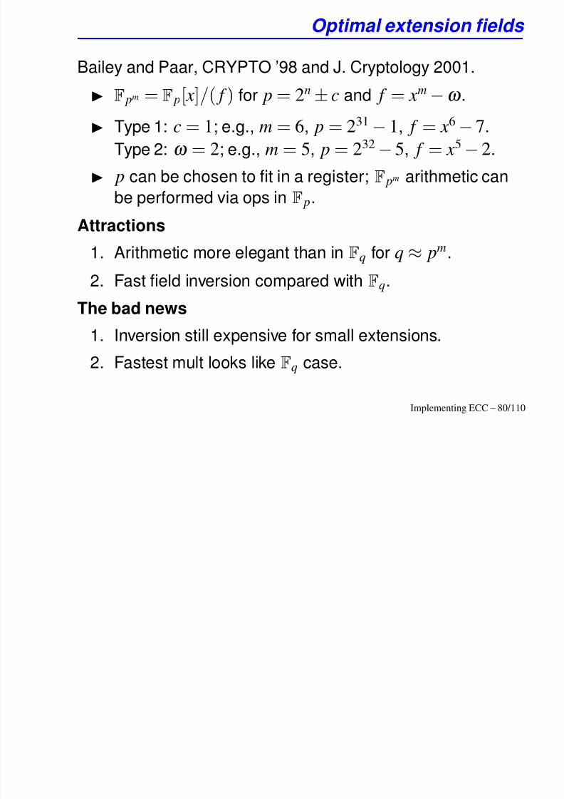
Bailey and Paar, CRYPTO ’98 and J. Cryptology 2001.



F pm = F p[ x]/( f ) for p = 2n ± c and f = xm −ω .

Type 1: c = 1; e.g., m = 6, p = 231 − 1, f = x6 − 7.

Type 2: ω = 2; e.g., m = 5, p = 232

−5, f = x5

−2.

p can be chosen to fit in a register; F pm arithmetic can

be performed via ops in F p.

Attractions

1. Arithmetic more elegant than in Fq for q ≈ pm.

2. Fast field inversion compared with Fq.

The bad news1. Inversion still expensive for small extensions.

2. Fastest mult looks like Fq case.


Inversion in OEFs (Itoh & Tsujii)

Given A F pm and r = pm−1

p 1= pm−1 + + p + 1, find



∈p

− · · · A−1 = ( Ar )−1 Ar −1.

Steps

1. Compute Ar −

1

= A pm

−1+

···+ p

.2. Ar = Ar −1 A ∈ F p.

3. Find c = ( Ar )−1 in F p.

4. A−1

= cAr

−1

.Cost

Steps 1 and 3 appear to be the expensive calculations.

Step 2 is not a full field multiplication. Step 3 is inversion in F p, which is relatively fast.

Step 1 can be done with a few field multiplications.


Direct inversion for m = 2

Let a = a0 + a1 x, f ( x) = x2 ω , ω F p. Want



− ∈a−1 = a0 + a1 x.

aa−1 ≡ 1 (mod f ) gives

a0 ω a1

a1 a0a

0a

1 = 1

0 .

Then

a−1

= (a0,−a1)/∆

,∆

= a

2

0 −ω a

2

1.Cost: I + 2 M + 2S (and a mult by ω ), all in the subfield.


Extending OEF: tower fields

Idea: do a sequence of extensions with f i( x) = xt ω i−1



−irreducible over GF (qt i−1) and f i(ω i) = 0.

Main attraction: faster inversion than in OEF.

OEF subfield inversion may require 40% of the total

inversion time. Recursion in OTF =⇒ subfieldinversion in Fq is expected to be less expensive.

The bad news

1. Multiplication slightly slower.

2. Unclear if inversion is fast enough to favor affine coords.

3. Analysis is limited. Parameters chosen (on ARM) mayfavor method.

4. Security of curves over OEFs and OTFs needs more

analysis.

Baktir and Sunar [IEEE ToC 2004]. Implementing ECC – 83/110

Processor Adequate Finite Fields

Avanzi and Mihailescu [SAC 2003] discuss PAFFs.



Similar to OEF, but p may be any prime subject to sizerestriction (size chosen to cooperate with hardware).

Use “partial reduction” to reduce cost. Redundant rep.

Redundant reps and partial reduction is a widely-used

technique.

1. Bernstein’s fast floating-point implementations for F p.

2. Fields with parameters not-of-special-form.

Gura, Eberle, and Chang Shantz, for F2m .

Yanik, Savas, and Koç, for F p.

Techniques have some application for special-form

parameters.


Move to a friendlier ring

Idea: move to a ring where where arithmetic is more



pleasant.

Specialized case with fields having a type 1 ONB is

well-known.

Map field elts to F2[ x]/( f ) where f = xm+1

− 1 x − 1

.

Do most arithmetic modulo xm+1 − 1.

Limitations: must have m + 1 prime. Type 1 ONBs

relatively rare.

Technique generalizes to Gaussian bases of type T , but with

factor T expansion.


Move to a friendlier ring

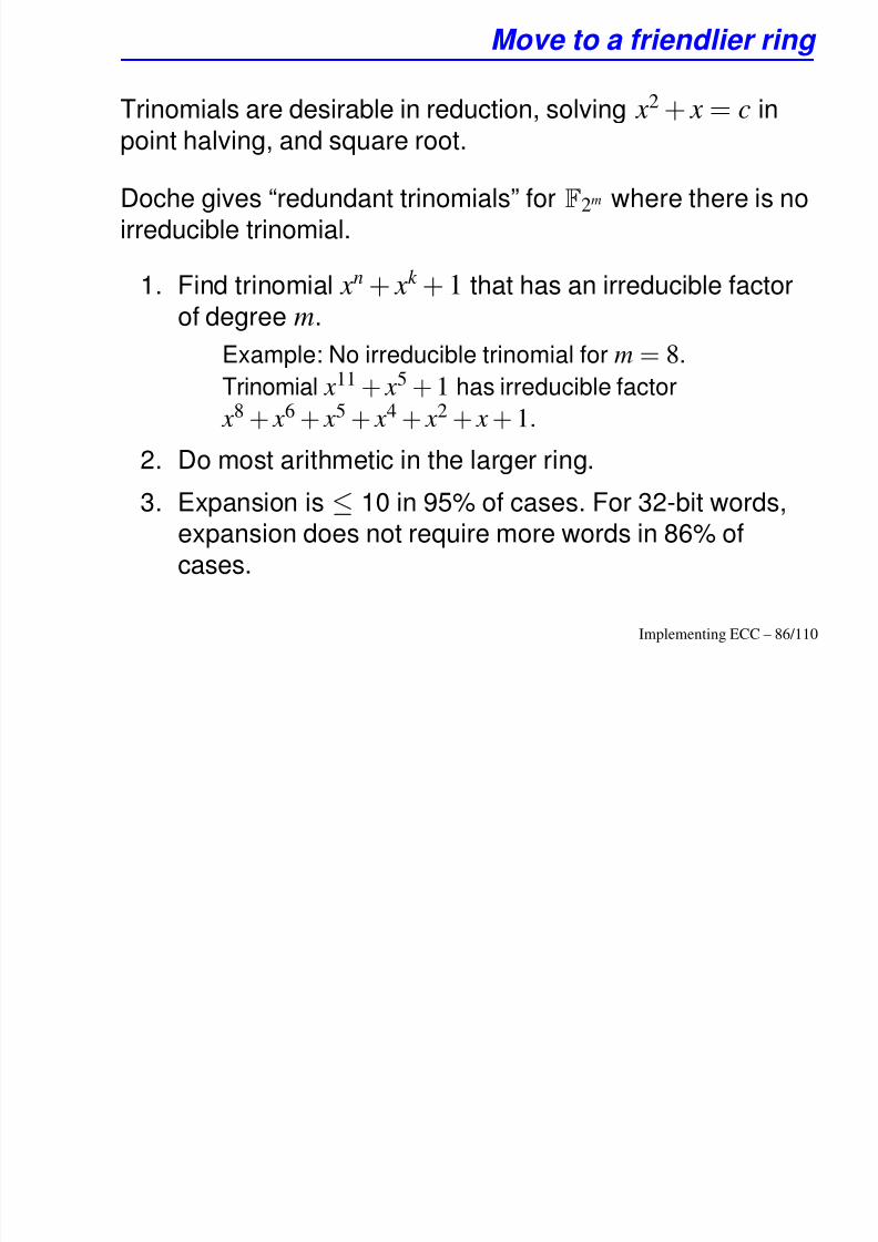
Trinomials are desirable in reduction, solving x2 + x = c in



point halving, and square root.

Doche gives “redundant trinomials” for F2m where there is no

irreducible trinomial.

1. Find trinomial xn + xk + 1 that has an irreducible factor

of degree m.

Example: No irreducible trinomial for m = 8.

Trinomial x11 + x5 + 1 has irreducible factor

x8 + x6 + x5 + x4 + x2 + x + 1.

2. Do most arithmetic in the larger ring.

3. Expansion is ≤ 10 in 95% of cases. For 32-bit words,expansion does not require more words in 86% of

cases.


Move to a friendlier ring...

4. Optimal redundant trinomials have degree divisible by

32



32.Example: x197+27 + x103 + 1 has irreducible factor

of degree 197.

Faster, even though extension is usually larger. Optimal

quadrinomials more common.

5. 20% improvement for reductions and squarings. Less

than 5% for multiplications.

6. Inversion 15% slower.

Implementation was with NTL. More experimental data

desirable.


Hyperelliptic curves

Hyperelliptic curve of genus g over Fq:

2 h( ) f ( )



v2 + h(u)v = f (u)

h, f ∈ Fq[u], deg f = 2g + 1, deg h ≤ g.

g = 1 =⇒ elliptic curve. Known attacks =⇒ g ≤ 4 (or g ≤ 3) of interest.

Arithmetic is in smaller fields for g ∈ {2, 3}, but curve

operations are more complicated. Significant improvements in explicit formulae by Lange,

Pezl, Wollinger, Guarjardo, Paar.


Hyperelliptic vs elliptic curves

1. Avanzi [CHES 2004]: roughly 15% penalty with genus 2

i fi ld d ith EC



curves over prime fields compared with EC.

Limitations: “not interested in...prime moduli of special

form” but this is a comparison of interest and may favor

elliptic curves.

2. Lange and Stevens [SAC 2004]: genus 2 curves with

degh = 1 are competitive or faster than EC for curves

over binary fields.

Limitations: implementation was with NTL. Affine

coords only.


References

1. R. Avanzi. Aspects of hyperelliptic curves over large prime

fields in software implementations CHES 2004 LNCS



fields in software implementations. CHES 2004, LNCS3156:148–162.

2. Avanzi and P. Mihailescu. Generic efficient arithmetic

algorithms for PAFFs (Processor Adequate Finite Fields)

and related algebraic structures. SAC 2003, LNCS

3006:320-334, 2004.

3. S. Baktir and B. Sunar. Optimal tower fields. IEEE

Transactions on Computers 53:1231–1243, 2004.

4. C. Doche. Redundant trinomials for finite fields of

characteristic 2. Cryptology ePrint Archive

http://eprint.iacr.org/2004/055/ .


References...

5. T. Kobayashi, H. Morita, K. Kobayashi, F. Hoshino. Fast

elliptic curve algorithm combining frobenius map and table





elliptic curve algorithm combining frobenius map and tablereference to adapt to higher characteristic. EUROCRYPT

’99, LNCS 1592:176-189. [Koblitz-like speedups. Downside:

curve is over large subfield.]

6. V Müller. Efficient point multiplication for elliptic curves over

special optimal extension fields. Public-Key Cryptography

and Computational Number Theory, pages 197–207, de

Gruyter, 2001. [Combines the ideas of GLV and OEF.]7. T. Yanik, E. Savas, and Ç. Koç. Incomplete reduction in

modular arithmetic. IEE Proceedings: Computers and

Digital Techniques, 149(2):46-52, March 2002.


Topic VI



Using special-purpose hardware


Case study: the Intel x86 (Pentium) family

Outline

1 Declining performance of integer arithmetic with



1. Declining performance of integer arithmetic withgeneral-purpose registers.

2. The floating-point approach.

3. “Multimedia” single-instruction multiple-data (SIMD)hardware.

4. Wish list: special instructions.


Intel IA-32 processors

Processor Year Selected features

386 1985 First IA-32 family processor with 32-bit operations and par-



386 1985 First IA 32 family processor with 32 bit operations and parallel stages.

486 1989 5 pipelined stages in the 486; processor is capable of one

instruction per clock cycle.

Pentium

Pentium MMX

1993

1997

Dual-pipeline: optimal pairing gives two instructions per

clock cycle. MMX added eight special-purpose 64-bit “mul-

timedia” registers, supporting operations on vectors of 1, 2,

4, or 8-byte integers.

Pentium Pro

Pentium II

Celeron

Pentium III

1995

1997

1998

1999

P6 architecture has more sophisticated pipelining and out-

of-order execution. Up to 3 µ-ops executed per cycle. Im-

proved branch prediction, but misprediction penalty much

larger than on Pentium. Integer multiplication faster. SSE

extensions on P-III have 128-bit registers supporting ops on

vectors of single-precision floating-point values.

Pentium 4 2000 NetBurst architecture runs at significantly higher clockspeeds, but many instructions have worse cycle counts

than P6 family processors. SSE2 extensions have double-

precision floating-point and 128-bit packed integer data

types.


Multiplication on the Pentium

The good news

Can do integer multiplication 32×32 → 64 bits



Can do integer multiplication 32×32 → 64 bits.

Pentium II/III have faster multiplication than originalPentium and MMX.

The bad news

Must use a and d registers for the mult of interest.

Multiplication on Pentium 4 with general-purpose

registers is slower than on earlier processors.

Pentium II/III have better branch prediction than the

original Pentium, but mispredictions are more

expensive.


Instruction latency/throughput

Latency/throughput for Pentium II/III vs Pentium 4

Instruction Pentium II/III Pentium 4



Instruction Pentium II/III Pentium 4Integer add, xor,... 1 / 1 .5 / .5

Integer add, sub with carry 1 / 1 6–8 / 2–3

Integer multiplication 4 / 1 14–18 / 3–5

Floating-point multiply 5 / 2 7 / 2

MMX ALU 1 / 1 2 / 2

MMX multiply 3 / 1 8 / 2

Latency: number of clock cycles required before the

result of an operation may be used.

Throughput: number of cycles which must pass before

the instruction may be executed again.

Small latency and small throughput are desirable.

Throughput can be significantly less than latency.


Faster multiplication: floating-point

Idea: use floating-point hardware to implement fast integer

arithmetic



arithmetic. Potential for broad applicability: DEC Alpha, Intel

Pentium, Sun SPARC, AMD Athlon.

IEEE double-precision floating-point formats e (11-bit exponent) f (52-bit fraction)

63 62 52 51 0

represents numbers z = (−1)s × 2e−1023 × 1. f .

Normalization of the significand 1. f increases effective

precision to 53 bits.

80-bit double-extended format.

Pentium has 8 floating-point registers. Length of the

significand is selected in a control register.


Floating-point

Some good news

Floating-point addition operates on more bits than



Floating point addition operates on more bits thanaddition with integer instructions on 32-bit hardware.

More registers and not restricted to specific registers.

Can do useful things during the latency period.

Some bad news

Expensive to move between integer and floating-point

formats.

Bit operations which are convenient in integer format

(e.g., extraction of specific bits, division by 2) are

clumsy on values in floating point registers. Redundant rep =⇒ tests for equality are more

expensive.


Scalar multiplication for P-224

Bernstein: minimize conversions to/from floating point.

P 224: NIST curve over F for prime p = 2224 296 + 1



P-224: NIST curve over F p for prime p = 2 −2 + 1.

Performance improvements are in field arithmetic (and

in the organization of field ops in point doubling and

addition).

Field multiplication will require more than 64

(floating-point) multiplications, compared with 49 in the

classical method. On the positive side, more registers are available, mult

can occur on any register, and products may be directly

accumulated in a register without handling carry.


P-224 field multiplication

Multiplication in F p2241.7 GHz P4

Classical integer 0.62

Karatsuba-Ofman 0.82



Floating-point 0.20a

aExcludes canonical form conversions.The good news

1. Wide applicability. No coding in assembly.2. Excluding conversions, can do c = ab (to 8 FP values

of roughly 28 bits) very fast.

The bad news1. No assembly required, but have to manage scheduling

and register allocation.

2. Can’t allow compiler to unexpectedly spill 80-bitextended-double to 64-bit doubles. Alignment.

3. Conversion to canonical form is expensive, so must

commit to FP across curve operations.

4. Algorithm verification. Implementing ECC – 100/110

P-224 Curve arithmetic

Bernstein uses a width-4 window method (without sliding) for

kP.( / )( / )



Expected 3 + (15/16)(224/4) point additions.

Scalar multiplication timings:

Cycles for kP

Method Pentium III Pentium 4

general-purpose registers 1,200,000 2,700,000

floating-point registers 730,000 830,000

Reference implementation processes k = ∑55i=0 k i24i where −8 ≤k i < 8. Precomp stores iP in Chudnovsky coords ( X :Y : Z : Z 2: Z 3) for

i ∈ [−8, 8).




Single-instruction multiple-data (SIMD)

Perform operations in parallel on vectors. All Intel Pentiums

except original and Pentium Pro.I iti ll “MMX T h l ” f lti di



p g Initially “MMX Technology” for multimedia.

Extension Registers Features added

MMX (PII) 8 64-bit vector ops on 1,2,4,8 byte integers;share space with floating-point reg-

isters

SSE (PIII) 8 128-bit vector ops on single-precision

floating-point

SSE2 (P4) 8 128-bit vector ops on double-precision float-

ing point and 64-bit integers

MMX suitable for binary field multiplication andinversion.

SSE2 provides integer alternative to floating-point

multiplication.Implementing ECC – 103/110

Single-instruction multiple-data (SIMD)

Advanced Micro Devices (AMD) K6 processor has

MMX.S h Vi l I t ti S t (VIS)



Sun has Visual Instruction Set (VIS).

Basic idea applied to Intel and AMD processors:

Implement fast 64-bit operations on primarily 32-bit

machines.

Gives more registers on register-poor machine.

Integer multiplication (SSE2) can use 8 registers

(32×32 multiply with general-purpose registers has

output in a and d ).

SSE2 integer multiply has latency 8 and throughput 2.Can do useful things in the latency period.


SIMD integer multiplication methods

Notation: integers a = ∑ai Bi for some B = 2w (e.g., w = 28

or w = 32). Want c = ab.



1. Operand scanning approach.

a0 a1 a2

b2 a0b2 · · · a1b2 · · · a2b2 → c +∑aib2 Bi+2

b1 a0b1 · · · a1b1 · · · a2b1 → c +∑aib1 Bi+1

b0 a0b0

· · ·a1b0

· · ·a2b0

→c +∑aib0 B

i+0

Advantages

Control code is simple.

Can use full 32-bit multiplications.

Downsides

More memory accesses if few registers available.

Must shift after each multiplication. Implementing ECC – 105/110

SIMD integer multiplication methods

2. Product scanning method.a0 a1 a2

b2 a0b2 a1b2 a2b2



2 0 2 1 2 2 2. . .

. . . b1 a0b1 a1b1 a2b1 ∑

i+ j=4

aib j B4

.. .

.. . b0 a0b0 a1b0 a2b0 ∑

i+ j=3

aib j B3

∑

i+ j=0

aib j B0 ∑

i+ j=1

aib j B1 ∑

i+ j=2

aib j B2

Advantages

Possibly fewer memory accesses.

Less shifting.

Downsides

Control code more complicated (unless fully unrolled).

To avoid carry, take w < 32. “Wastes” part of the

multiplier. Implementing ECC – 106/110

SIMD integer multiplication methods...

1. GNU mp uses operand scanning.

2. Moore uses vector ops in 128-bit SSE2 to compute twoproducts (with w = 29) simultaneously Roughly



products (with w = 29) simultaneously. Roughly

operand scanning, but carry is handled in 2nd stage.

3. To avoid the requirement w < 32 in product scanning,use shuffle instruction to split 64-bit product uv:

←− 64 bits −→ ←− 64 bits −→

0 · · ·0 0 · · ·0 uvhigh uvlow↓ pshufd

0 · · ·0 uvhigh 0 · · ·0 uvlow

and then accumulate. Downside: have to shuffle onevery mult.

Experiments suggest product scanning with scalar ops wins

(even though input must be split and output reassembled).Implementing ECC – 107/110

Multiplication with SSE2 integer ops

Multiplication in F p224Pentium 4 (1.7 GHz)

Classical integer (product scanning) 0.62Karatsuba-Ofman (depth 2) 0 82



Karatsuba Ofman (depth 2) 0.82

SIMD (SSE2; product scanning) 0.27

Floating-point 0.20a

aExcludes conversion to/from canonical form.

Floating-point includes partial reduction to 8floating-point values (each roughly 28 bits); does not

include expensive conversion to canonical reducedform. Other times include reduction.

Classical and Karatsuba would benefit from additional

tuning specific to Pentium 4; regardless, both will beinferior to SIMD and floating-point.

SIMD does not require the commitment of the

floating-point approach.


Summary: special-purpose hardware

1. Designs such as Pentium 4 and UltraSPARC have slow

integer mult with general-purpose registers.2 Common MMX subset suitable for binary field



2. Common MMX subset suitable for binary field

arithmetic. Relatively easy to code.

3. Floating-point hardware common on workstationsspeeds prime field arithmetic. Must commit to coding

across curve operations.

4. Integer SSE2 extensions on Pentium 4 easy to insert

locally, but not as fast as floating-point approach. Notavailable with Pentium II/III.

Wish list: Großschädl and Savas [CHES 2004] propose

instruction set extensions to speed field ops.

Amusements: use graphics card as a crypto co-processor

[CT-RSA 2005].


Hankerson-WIMC2005

Documents

Transcript of Hankerson-WIMC2005