
Handbook on decision making techniques and applications
548
-
Upload
shirazthegreat -
Category
Self Improvement
-
view
477 -
download
1
description
Handbook on decision making techniques and applications
Transcript of Handbook on decision making techniques and applications


Lakhmi C. Jain and Chee Peng Lim (Eds.)
Handbook on Decision Making: Techniques and Applications

Intelligent Systems Reference Library,Volume 4
Editors-in-Chief
Prof. Janusz KacprzykSystems Research InstitutePolish Academy of Sciencesul. Newelska 601-447 WarsawPolandE-mail: [email protected]
Prof. Lakhmi C. JainUniversity of South AustraliaAdelaideMawson Lakes CampusSouth Australia 5095AustraliaE-mail: [email protected]
Further volumes of this series can be found on our homepage: springer.com
Vol. 1. Christine L. Mumford and Lakhmi C. Jain (Eds.)Computational Intelligence: Collaboration, Fusionand Emergence, 2009ISBN 978-3-642-01798-8
Vol. 2.Yuehui Chen and Ajith AbrahamTree-Structure Based HybridComputational Intelligence, 2009ISBN 978-3-642-04738-1
Vol. 3.Anthony Finn and Steve SchedingDevelopments and Challenges forAutonomous Unmanned Vehicles, 2010ISBN 978-3-642-10703-0
Vol. 4. Lakhmi C. Jain and Chee Peng Lim (Eds.)Handbook on Decision Making: Techniquesand Applications, 2010ISBN 978-3-642-13638-2

Lakhmi C. Jain and Chee Peng Lim (Eds.)
Handbook on Decision Making
Vol 1: Techniques and Applications
123

Prof. Lakhmi C. JainUniversity of South Australia
School of Electrical &
Information EngineeringKES Centre
5095 Adelaide South Australia
Mawson Lakes CampusAustralia
E-mail: [email protected]
Dr. Chee Peng LimUniversity of Science Malaysia
School of Electrical andElectronic Engineering
Engineering Campus14300 Nibong Tebal, Penang
Malaysia
E-mail: [email protected]
ISBN 978-3-642-13638-2 e-ISBN 978-3-642-13639-9
DOI 10.1007/978-3-642-13639-9
Intelligent Systems Reference Library ISSN 1868-4394
Library of Congress Control Number: 2010928590
c© 2010 Springer-Verlag Berlin Heidelberg
This work is subject to copyright. All rights are reserved, whether the whole or partof the material is concerned, specifically the rights of translation, reprinting, reuseof illustrations, recitation, broadcasting, reproduction on microfilm or in any otherway, and storage in data banks. Duplication of this publication or parts thereof ispermitted only under the provisions of the German Copyright Law of September 9,1965, in its current version, and permission for use must always be obtained fromSpringer. Violations are liable to prosecution under the German Copyright Law.
The use of general descriptive names, registered names, trademarks, etc. in thispublication does not imply, even in the absence of a specific statement, that suchnames are exempt from the relevant protective laws and regulations and thereforefree for general use.
Typeset & Cover Design: Scientific Publishing Services Pvt. Ltd., Chennai, India.
Printed on acid-free paper
9 8 7 6 5 4 3 2 1
springer.com

Preface
Decision making arises when we wish to select the best possible course of action from a set of alternatives. With advancements of the digital technologies, it is easy, and almost instantaneous, to gather a large volume of information and/or data pertaining to a problem that we want to solve. For instance, the world-wide-web is perhaps the primary source of information and/or data that we often turn to when we face a decision making problem. However, the information and/or data that we obtain from the real world often are complex, and comprise various kinds of noise. Besides, real-world information and/or data often are incomplete and ambiguous, owing to uncertainties of the environments. All these make decision making a challenging task. To cope with the challenges of decision making, re-searchers have designed and developed a variety of decision support systems to provide assistance in human decision making processes.
The main aim of this book is to provide a small collection of techniques stemmed from artificial intelligence, as well as other complementary methodolo-gies, that are useful for the design and development of intelligent decision support systems. Application examples of how these intelligent decision support systems can be utilized to help tackle a variety of real-world problems in different do-mains, e.g. business, management, manufacturing, transportation and food indus-tries, and biomedicine, are also presented. A total of twenty chapters, which can be broadly divided into two parts, i.e., (i) modelling and design techniques for intelligent decision support systems; and (ii) reviews and applications of intelli-gent decision support systems, are included in this book. A summary of each chapter is as follows. Part I Modelling and Design Techniques for Intelligent Decision Support Systems An overview of intelligent decision making is presented in Chapter 1. The general aspects of decision making, decision quality, and types of decision support sys-tems are explained. A number of intelligent techniques stemmed from artificial intelligence that are useful for the design and development of intelligent decision support systems are described. Application examples of these intelligent tech-niques, as well as their hybrid models, are also highlighted.
In Chapter 2, an intelligent decision support systems engineering methodology for designing and building intelligent decision support systems is described. The proposed methodology comprises four phases: project initiation, system design, system building and evaluation, and user’s definitive acceptance. The usefulness of the proposed methodology is assessed in academic settings with realistic case

Preface VI
studies, and satisfactory results are reported. The implication of the proposed methodology in providing a systematic software engineering oriented process for users to develop intelligent decision making support systems is discussed.
In a highly competitive market, the design of products becomes a challenging task owing to diversified customer needs and complexity of technologies. In Chapter 3, a framework that describes the relationships of the product design problems, product design processes, shape design processes, shape design meth-ods and tools with consideration of the functional, ergonomic, emotional, and manufacturing requirements, is presented. A decision support system to assist designers in designing product shapes is developed. A case study on scooter shape design is conducted. Applicability of the decision support system to plan-ning the shape design process and creating a scooter shape following the planned processes is demonstrated.
A Tree-based Neural Fuzzy Inference System (TNFIS) for model formulation problems in time series forecasting, system identification, as well as classification problems is suggested in Chapter 4. The proposed approach takes the imprecise nature of decision makers' judgements on the different tacit models into considera-tion. The learning algorithm of the TNFIS consists of two phases: Piaget's action-based structural learning phase, and a parameter tuning phase. Knowledge in the form of fuzzy rules is created using the TNFIS, and visualization techniques are proposed so that the decision maker can better understand the formulated model. The effectiveness of the TNFIS is demonstrated using benchmark problems.
A general approach to decision making in complex systems using agent-based decision support systems is described in Chapter 5. The approach contributes to decentralization and local decision making within a standard work flow. A layered structure is adopted to address issues involving (i) data retrieval, fusion, and pre-processing; (ii) data mining and evaluation; and (iii) decision making, alerting, solutions and predictions generation. The agent-based decision support system is applied to evaluate the impact of environmental parameters upon human health in a Spanish region. It is found that the system is able to provide all the necessary steps for decision making by using computational agents.
In Chapter 6, single-criterion and multiple-criteria decision analysis for sustain-able rural energy policy and planning is described. A number of single-criterion and multiple-criteria energy decision support systems are analysed, with their strengths and limitations discussed. A sustainable rural energy decision support system, which combines quantitative and qualitative criteria and enables the pri-orities of a group of prospective users to be considered in decision analysis, is described. Novelty of the decision support system lies in its ability to match rural community’s needs in developing countries to appropriate energy technologies, thereby improving livelihoods and sustainability. A study on using the decision support system for energy analysis and planning of a remote community in Co-lombia is presented.
It is argued that decision making is the bridge between sensation and action, i.e. the bridge between processing of stimulus input and generation of motor output. In Chapter 7, a decision making model known as the complementary decision making system is proposed. The model is based complementary learning that

Preface VII
functionally models the lateral inhibition and segregation mechanisms observed in the human decision making process, i.e., in prefrontal and parietal lobes neural basis of decision making. Fuzzy rules are generated to inform users how confi-dent the system is in its predictions. To assess the performance of the proposed model, a number of benchmark medical data sets are used. The results compared favourably with those from other machine learning methods.
A variety of forecasting techniques are used by a lot of major corporations to predict the uncertain future in an attempt to make better decisions which affect the future of the organizations. In Chapter 8, a forecasting support system based on the exponential smoothing scheme for forecasting time-series data is presented. Issues related to parameter estimation and model selection are discussed. A Bayesian forecasting support system, i.e., SIOPRED-Bayes, is described. The system incorporates existing univariate exponential smoothing models as well as some generalizations of these models in order to deal with features arising in eco-nomic and industrial scenes. Its application to water consumption forecasting is demonstrated.
Partially observable Markov decision processes provide a useful mathematical framework for agent planning under stochastic and partially observable environ-ments. In Chapter 9, a memory-based reinforcement learning algorithm known as reinforcement-based U-Tree is described. It is able to learn the state transitions from experience and build the state model by itself based on raw sensor inputs. Modifications to U-Tree’s state generation procedure to improve the effectiveness of the state model are also proposed. Its performance is evaluated using a car-driving task. In addition, a modification to the statistical test for reward estima-tion is suggested, which allows the algorithm to be benchmarked against some model-based approaches with well-known problems in partially observable Markov decision processes.
The Fuzzy Inference System (FIS) has been demonstrated to be a useful model in undertaking a variety of assessment and decision making problems. In Chapter 10, the importance of the monotonicity property of an FIS-based assessment model is investigated. Specifically, the sufficient conditions for an FIS-based assessment model to satisfy the monotonicity property are derived. In addition, a Failure Mode and Effective Analysis (FMEA) framework with an FIS-based Risk Priority Number (RPN) model is examined. A case study of the applicability of the FMEA framework to a semiconductor manufacturing process is conducted. The results obtained indicate the importance of the monotonicity property of the FIS-based RPN model in tackling assessment and decision making problems. Part II Reviews and Applications of Intelligent Decision Support Systems A thorough study on the use of decision support systems in the transportation industry is presented in Chapter 11. A taxonomy for classifying transportation decision support systems is described. The usefulness of transportation decision support systems in solving different types of decision problems is examined. Methodologies of decision making as well as information technologies that are useful for developing transportation decision support systems are also discussed.

Preface VIII
A useful review on a large variety of decision support systems that are applied to different transportation sectors, which cover road, urban, air, rail, and seaborne transportation, is included.
Application of decision support systems to the food industry, and in particular the seafood industry, is presented in Chapter 12. The food industry is different to many other industries, since the nature of the products and ingredients can change dramatically with time. Traceability is important in order to know the history of the product and/or ingredient of interest. By exploiting product traceability, the flow of data can be used for decision support. It is pointed out that decision sup-port systems are beneficial to a number of areas in food processing, which include lowering environmental impact of food processing, safety management, process-ing management, and stock management. The usefulness of decision support systems for the meat industry, food producers, inventory management and replen-ishment for retailers are also described.
Creative city design is a multi-facet problem which involves a wide range of knowledge and a diverse database. Based on rough sets, a decision support sys-tem that is able to help decision-makers leverage resources with information tech-nology for creative city design is presented in Chapter 13. The design rules of creative city development by urban design experts are also described. Rough set theory is applied to select the decision rules and measure the current status of Japanese cities. A prototype, i.e., Urban Innovators Systems, to demonstrate the usefulness of the approach in building a collaborative model of creative city with public participation is discussed.
A major aspect of decision making is in making buying and selling decisions. In Chapter 14, a combinatorial auction mechanism where bidders can submit mul-tiple prices (pessimistic, ideal, and optimistic values) in a single package is de-scribed. A new operationalization on the auctioneer-bidder relationship based on the type of bids or triangular possibility distribution is proposed. The proposed approach is evaluated with test problems in a fuzzy auction environment. The analysis reveals that the fuzzy solution interval provides both negotiation and risk assessment capability for the auctioneer.
Accidental building fires cause many fatalities and property losses to the com-munity. Artificial neural networks have been shown to be an efficient and effec-tive decision making models in fire safety applications. In Chapter 15, a hybrid neural network model that combines Fuzzy ART and the General Regression Neural Network is proposed. A series of experiments using benchmark datasets to examine the usefulness of the network in tackling general data regression prob-lems is first conducted. A novel application of the proposed hybrid network to predicting evacuation time during fire disasters is described. The results demon-strate the efficacy of the proposed network in undertaking fire safety engineering problems.
In Chapter 16, the use of the path-converged design, which is a nonparametric approach, for decision making in optimal migration strategy in urban planning is examined. A study to identify existing population agglomeration for small, me-dium, and large cities from both regional and urban perspectives and to evaluate the efficiency of existing population agglomeration in urban planning is first

Preface IX
conducted. Identification based on path-converged design reveals inefficiency in existing population agglomeration in China. Based on the identified population agglomeration and the inefficiency of agglomeration, a number of population migra-tion decisions to eliminate inefficiency of population allocation are discussed.
In Chapter 17, the use of a number of fuzzy neural networks to superficial ther-mal images against the true internal body temperature is described. Comparison between global and local semantic memories as well as Mamdani and Takagi-Sugeno-Kang model of fuzzy neural networks are presented. A series of experimen-tal studies using real data from screening of potential SARS patients is conducted. The experimental results of temperature classification based on thermal images are analysed. A comparison between various global and local learning networks is pre-sented. The outcomes demonstrate the potential of fuzzy neural networks as an intel-ligent medical decision support tool for thermal analysis, with the capability of yielding plausible semantic interpretation of the system prediction to domain users.
Electroencephalogram (EEG) is one of the most important sources of informa-tion in therapy of epilepsy, and researchers have addressed the issue of engaging decision support tools for such a data source. In Chapter 18, the application of a novel fuzzy logic system implemented in the framework of a neural network for classification of EEG signals is presented. The proposed network constructs its initial rules by clustering while the final fuzzy rule base is determined by competi-tive learning. Both error backpropagation and recursive least squares estimation techniques are used for tuning premise and consequence parameters of the net-work. Applicability of the network to EEG signal classification is demonstrated.
In Chapter 19, a case base reasoning system for differentiation based on altered control of saccadic eye movements in Attention-Deficit Hyperactivity Disorder (ADHD) subjects and a control group is described. The TA3 system, an intelli-gent decision support system that incorporates case based reasoning into its framework, is used to retrieve and apply previous ADHD diagnostic cases to novel problems based on saccade performance data. The results demonstrate that the proposed system is able to distinguish ADHD from normal control subjects, based on saccade performance, with increasing accuracy.
In Chapter 20, the use of a brain inspired, cerebellar-based learning memory model known as pseudo self-evolving cerebellar model articulation controller to model autonomous decision-making processes in dynamic and complex environ-ments is described. The model adopts an experience-driven memory management scheme, which has been demonstrated to be more efficient in capturing the inher-ent characteristics of the problem domain for effective decision making. Applica-bility of the model is evaluated using dynamics of the metabolic insulin regulation mechanism of a healthy person when perturbed by food intakes. The model is use-ful for capturing complex interacting relationships of the blood glucose level, the food intake, and the required blood insulin concentration for metabolic homeostasis.

Preface X
The editors would like to express their utmost gratitude and appreciation to the authors for their contributions. The editors are grateful to the reviewers for their constructive comments and suggestions in improving the quality of each chapter presented in this book. Thanks are also due to the excellent editorial assistance by staff at Springer-Verlag. Chee Peng Lim
Lakhmi C. Jain

Table of Contents
Part I: Modelling and Design Techniques forIntelligent Decision Support Systems
Chapter 1Advances in Intelligent Decision Making . . . . . . . . . . . . . . . . . . . . . . . . . . 3
Chee Peng Lim, Lakhmi C. Jain
Chapter 2IDSSE-M: Intelligent Decision Support Systems EngineeringMethodology . . . . . . . . . . . . . . . . . . . . . . . . . . . . . . . . . . . . . . . . . . . . . . . . . . 29
M. Mora, G. Forgionne, F. Cervantes-Perez, O. Gelman
Chapter 3Shape Design of Products Based on a Decision SupportSystem . . . . . . . . . . . . . . . . . . . . . . . . . . . . . . . . . . . . . . . . . . . . . . . . . . . . . . . 55
Yung-chin Hsiao, Junzo Watada
Chapter 4Enhancing Decision Support System with Neural FuzzyModel and Simple Model Visualizations . . . . . . . . . . . . . . . . . . . . . . . . . . . 85
Eng Yeow Cheu, See Kiong Ng, Chai Quek
Chapter 5Computational Agents in Complex Decision Support Systems . . . . . . . . 117
Antonio Fernandez-Caballero, Marina V. Sokolova
Chapter 6A Multi-criteria Decision-Support Approach to SustainableRural Energy in Developing Countries . . . . . . . . . . . . . . . . . . . . . . . . . . . . 143
Judith A. Cherni, Nicole Kalas
Chapter 7A Decision Making System Based on ComplementaryLearning . . . . . . . . . . . . . . . . . . . . . . . . . . . . . . . . . . . . . . . . . . . . . . . . . . . . . . 163
Tuan Zea Tan, Geok See Ng, Chai Quek

XII Table of Contents
Chapter 8A Forecasting Support System Based on ExponentialSmoothing . . . . . . . . . . . . . . . . . . . . . . . . . . . . . . . . . . . . . . . . . . . . . . . . . . . . 181
Ana Corberan-Vallet, Jose D. Bermudez, Jose V. Segura,Enriqueta Vercher
Chapter 9Reinforcement Based U-Tree: A Novel Approach for SolvingPOMDP . . . . . . . . . . . . . . . . . . . . . . . . . . . . . . . . . . . . . . . . . . . . . . . . . . . . . . 205
Lei Zheng, Siu-Yeung Cho, Chai Quek
Chapter 10On the Use of Fuzzy Inference Systems for Assessment andDecision Making Problems . . . . . . . . . . . . . . . . . . . . . . . . . . . . . . . . . . . . . . 233
Kai Meng Tay, Chee Peng Lim
Part II: Reviews and Applications of IntelligentDecision Support Systems
Chapter 11Decision Support Systems in Transportation . . . . . . . . . . . . . . . . . . . . . . . 249
Jacek Zak
Chapter 12Decision Support Systems for the Food Industry . . . . . . . . . . . . . . . . . . . 295
Sigurjon Arason, Eyjolfur Ingi Asgeirsson, Bjorn Margeirsson,Sveinn Margeirsson, Petter Olsen, Hlynur Stefansson
Chapter 13Building a Decision Support System for Urban DesignBased on the Creative City Concept . . . . . . . . . . . . . . . . . . . . . . . . . . . . . . 317
Lee-Chuan Lin, Junzo Watada
Chapter 14Fuzzy Prices in Combinatorial Auction . . . . . . . . . . . . . . . . . . . . . . . . . . . 347
Joshua Ignatius, Seyyed Mahdi Hosseini Motlagh,M. Mehdi Sepheri, Young-Jou Lai, Adli Mustafa
Chapter 15Application of Artificial Neural Network to Fire SafetyEngineering . . . . . . . . . . . . . . . . . . . . . . . . . . . . . . . . . . . . . . . . . . . . . . . . . . . 369
Eric Wai Ming Lee

Table of Contents XIII
Chapter 16Decision-Making for the Optimal Strategy of PopulationAgglomeration in Urban Planning with Path-Converged Design . . . . . . 397
Bing Xu, Junzo Watada
Chapter 17A Cognitive Interpretation of Thermographic Images UsingNovel Fuzzy Learning Semantic Memories . . . . . . . . . . . . . . . . . . . . . . . . . 427
C. Quek, W. Irawan, E. Ng
Chapter 18Adaptive Fuzzy Inference Neural Network System for EEGSignal Classification . . . . . . . . . . . . . . . . . . . . . . . . . . . . . . . . . . . . . . . . . . . . 453
Pari Jahankani, Vassilis Kodogiannis, John Lygouras
Chapter 19A Systematic Approach to the Design of a Case-BasedReasoning System for Attention–Deficit Hyperactivity Disorder . . . . . . 473
Donald C. Brien, Janice I. Glasgow, Douglas P. Munoz
Chapter 20A NeuroCognitive Approach to Decision Making for theReconstruction of the Metabolic Insulin Profile of a HealthyPerson . . . . . . . . . . . . . . . . . . . . . . . . . . . . . . . . . . . . . . . . . . . . . . . . . . . . . . . . 497
S.D. Teddy, F. Yap, C. Quek, E.M.-K. Lai
Author Index . . . . . . . . . . . . . . . . . . . . . . . . . . . . . . . . . . . . . . . . . . . . . . . . 533


Part I
Modelling and Design Techniques for Intelligent Decision Support Systems


L.C. Jain and C.P. Lim (Eds.): Handbook on Decision Making, ISRL 4, pp. 3–28. springerlink.com © Springer-Verlag Berlin Heidelberg 2010
Chapter 1
Advances in Intelligent Decision Making
Chee Peng Lim1 and Lakhmi C. Jain2
1 School of Electrical & Electronic Engineering University of Science Malaysia, Malaysia
2 School of Electrical & Information Engineering University of South Australia, Australia
Abstract. In this chapter, an overview to techniques and applications re-lated to intelligent decision making is presented. The decision making process and elements of decision quality are discussed. A taxonomy of de-cision support systems is described. Techniques stemmed from artificial in-telligence that are useful for designing and development intelligent decision support systems are explained. The application of intelligent decision sup-port systems to a variety of domains is highlighted. A summary of conclud-ing remarks is presented at the end of this chapter.
1 Introduction
Decision support systems, in general, are a specific class of computerized infor-mation systems that supports decision-making activities in various domains, e.g. agriculture, biotechnology, finance, banking, manufacturing, healthcare, educa-tion, and government. A concise description of decision support systems is pro-vided in [pp.25, 1], as quoted:
“decision support systems are technologies that help get the right knowledge to the right decision makers at the right times in the right representations at the right costs.”
Indeed, we face a variety of decision making tasks in our daily life. We are pre-sented with a lot of information and/or data in our daily activities, and we, either consciously or sub-consciously, have to make decisions based on the received information and/or data. This situation is exacerbated by the world-wide-web as a resource for information and knowledge sharing and reuse. While there are many heterogeneous information and/or data sources on the world-wide-web, ranging from text documents to multi-media images; from audio files to video streams, the information and/or data often are complex and multi-facet, and comprise various kinds of noise. As such, we have to make a decision on the best possible course of action (or a set of optimized actions) from the available alternatives. However,

4 C.P. Lim and L.C. Jain
making a good and accurate decision is a challenging task. This is because con-flicts and tradeoffs often occur owing to multiple objectives and goals that are to be simultaneously satisfied by the decision maker. Hence, it is beneficial if some intelligent decision support system can be employed to assist us in making prompt and informed decisions.
According to [2], the concept of decision support stemmed from two main re-search areas: (i) theoretical studies of organizational decision making at the Carnegie Institute of Technology in the late 1950s/early 1960s; (ii) technical development of interactive computer systems mainly at the Massachusetts Insti-tute of Technology in the 1960s. Nevertheless, the advent of digital technolo-gies and information processing techniques to support problem solving and decision making tasks has further resulted in the emergence of intelligent deci-sion support systems. Indeed, decision support systems have evolved substan-tially and many new techniques like data warehouses, OLAP, data mining and web technologies have been incorporated into the design and development of decision support systems since the early 1970s [3]. As described in [4], infor-mation technology systems based on spreadsheet software have been deployed to support decision making activities in the 1970s. In the 1980s, optimization models from operation research and management science research have been incorporated to design decision support systems. In the 1990s, techniques from artificial intelligence and statistics have further enhanced the design and appli-cability of decision support systems.
What then constitute a successful intelligent decision support system? Six at-tributes that represent the high-level characteristics of successful decision support systems are discussed in [5]. They are (i) interactivity: the decision support sys-tem works well with others, which include other databases as well as human users; (ii) event and change detection: the decision support system monitors and recog-nizes important changes and events; (iii) representation aiding: the decision support system represents and communicates information effectively in a human-centred way; (iv) error detection and recovery: the decision support system checks for errors made by users, and, at the same time, knows its own limitations; (v) information out of data: the decision support system uses intelligent techniques to extract useful information from voluminous data and to handle outliers as well as other ambiguities in data sources; (vi) predictive capabilities: the decision support system assesses the effects of changes and predicts the impacts on future perform-ance, either on a short-term (tactical prediction) or long-term (strategic prediction) basis.
The organisation of this chapter is as follows. In section two, some general as-pects pertaining to the decision making process, elements that are useful to gauge decision quality, and a taxonomy of decision support systems are described. In section three, a number of artificial intelligence-based techniques that are useful for the design and development of intelligent decision support systems are pre-sented. The applicability of these intelligent decision support systems to a variety

Advances in Intelligent Decision Making 5
of different domains is discussed in section four. A summary of concluding re-marks is given in section five.
2 General Aspects of Decision Making
In this section, general aspects pertaining to decision making process, decision quality, and types of decision support systems are described, as follows.
2.1 The Decision Making Process
Over the years, a number of paradigms to describe the human decision making process have been proposed. Among them, the paradigm proposed by Simon (a Nobel laureate) [6] is widely tested and used [7, 8]. It consists of three phases, i.e., intelligence, design, and choice. Later, another implementation phase to Simon’s paradigm is added, as shown in Figure 1 [9, 10]. In the intelligence phase, a decision maker observes the reality, and establishes an understanding of the problem domain and the associated opportunities. The necessary information pertaining to all aspects of the problem under scrutiny is also collected. In the design phase, the decision criteria and alternatives are developed by using a spe-cific model, with the relevant uncontrollable events identified. The relationships between the decisions, alternatives and events have to be clearly specified and measured. This enables the decision alternatives to be evaluated logically in the next phase, i.e., the choice phase. Besides, actions that best meet the decision criteria are formulated. In the implementation phase, the decision maker needs to re-consider the decision analyses and evaluations, as well as to weigh the conse-quences of the recommendations. An implementation plan is then developed, with the necessary resources secured. It is now ready to put the implementation plan into action.
Notice that the decision making process is a continuous one within a feedback loop. This means that the decision maker should constantly re-consider and re-evaluate the reality and changes in the problem domain. Upon obtaining new information, it is necessary to re-visit one or more, if not all, of the four phases involved. The feedback process allows alterations and improvements on previous decisions to be accomplished, so as to meet the current needs and demands of the problem domain.
2.2 Decision Quality
In accordance with [11], the types of decisions can be broadly categories into two, i.e., operational decisions and strategic decisions. Operational decisions are con-cerned with managing operations, which are focused results on a short-term basis. The outcome of an operational decision, i.e., whether or not the decision is a good one, is known fairly quickly. The decision making process also attends to details and normally ignores uncertainty and avoids new alternatives[11].

6 C.P. Lim and L.C. Jain
Fig. 1. The decision making process (Source: [9])
On the other hand, strategic decisions involve predictions pertaining to impor-tant issues on a long-term basis. The decision making process takes uncertainty into consideration, and chooses among significantly different alternatives. While the quality of operational decisions can be judged from the short-term results, strategic decisions normally involve payoffs far into the future. In other words, it is difficult to judge the quality of strategic decision by the outcomes, which in-volve uncertainties in long time horizons. As such, a set of measures of decision quality is introduced in [11], as shown in Figure 2. There are six elements of
INTELLIGENCE • Observe reality • Gain problem/opportunity understanding • Acquire needed information
DESIGN • Develop decision criteria • Develop decision alternatives • Identify relevant uncontrollable events • Specify the relationships between criteria, alterna-
tives, and events • Measure the relationships
CHOICE • Logically evaluate the decision alternatives • Develop recommended actions that best meet the
decision criteria
IMPLEMENTATION • Ponder the decision analyses and evaluations • Weigh the consequences of the recommendations • Gain confidence in the decision • Develop an implementation plan • Secure needed resources • Put implementation plan into action

Advances in Intelligent Decision Making 7
decision quality, i.e., (i) appropriate frame; (ii) creative, doable alternatives; (iii) meaningful, reliable information; (iv) clear values and trade-offs; (v) logically correct reasoning; and (vi) commitment to action. Each element of the decision quality is discussed as follows, and the details are available in [11].
Fig. 2. Elements of decision quality (source: [11])
(i) Appropriate frame: As strategic decisions normally result in major, long-
term consequences, a team of decision makers from different background is required in the decision making process. As a result, an appropriate frame has to be established, with a clear purpose, conscious perspective, and de-fined scope.
(ii) Creative, doable alternatives: Owing to the nature of uncertainty, making a strategic decision needs to consider a lot of alternatives. It is therefore vital to explore all possibilities and to understand fully different alternatives that are available before making a decision. Quality is achieved when a number of different innovative and realizable alternatives are established for consideration.
(iii) Meaningful, reliable information: Information quality is very important in influencing strategic decisions. The team of decision makers ought to estab-lish correct and explicit information based on appropriate facts. The uncertainty involved can then be expressed in the form of a probabilistic judgement.
Meaningful, Reliable Information
Commitment to Action
Appropriate Frame
Creative, Doable
Alternatives
Logically Correct
Reasoning
Clear Values and
Trade-offs
Elements of Decision Quality

8 C.P. Lim and L.C. Jain
(iv) Clear values and trade-offs: Strategic decisions need to take into account a variety of trade-offs, which include trade-offs between present and future re-turns, trade-offs between risk and certainty, as well as trade-offs among dif-ferent criteria. As such, explicit statements of fundamental values need to be established.
(v) Logically correct reasoning: As strategic decisions are complex in nature, consequences of each alternative on the value measure should be evaluated comprehensively. In this case, a clear choice of the frame, alternatives, in-formation, and values is necessary in order to allow logical reasoning to be conducted.
(vi) Commitment to action: In any decision making process, a full commitment to put the action plan into implementation is a significant factor of ensuring success. Without commitments from all parties involved, it is unlikely to obtain any useful and beneficial results, even with the most sophisticated and comprehensive action plan in hand.
2.3 A Taxonomy of Decision Support Systems
In [12, 13] five different types of decision support systems, i.e., communication-driven, data-driven, document-driven, knowledge-driven, and model-driven, are proposed. A brief description of each type of decision support systems is as follows.
(i) Communication-drive decision support systems: the target group of these
decision support systems is the internal teams, which include partners, in an organisation to establish an efficient collaboration, e.g. a successful meet-ing. A web or client server is the most common technology used to deploy these decision support systems.
(ii) data-driven decision support systems: these systems are useful for querying a database or data warehouse to seek specific answers for specific purposes. They can be deployed using a mainframe system, client/server link, or via the web.
(iii) document-driven decision support systems: these systems are used to search web pages and find documents on a specific set of keywords or search terms. They can be implemented via the web or a client/server system;
(iv) knowledge-driven decision support systems: these cover a broad range of paradigms in artificial intelligence to assist decision makers from different domains. Various data mining techniques, which include neural networks, fuzzy logic, evolutionary algorithm, case-based reasoning, can be utilized for developing these systems to provide specialized expertise and informa-tion for undertaking specific decision making problems. They can be de-ployed using client/server systems, the web, or software running on stand-alone computers;
(v) model-driven decision support systems: these are complex systems devel-oped based on some model (e.g. mathematical and analytical models) to help analyse decisions or choose between different alternative. They can be deployed via software/hardware in stand-alone computers, client/server sys-tems, or the web.

Advances in Intelligent Decision Making 9
3 Techniques for Intelligent Decision Making
The types of decision support systems covered in this book mainly consist of knowledge-driven and model-driven systems. As such, a number of useful para-digms under the umbrella of artificial intelligence that have been widely used to design and develop intelligent decision support systems are described in the this section. These include artificial neural networks, evolutionary computing, fuzzy systems, case-based reasoning, and agent-based systems.
3.1 Artificial Neural Networks
Artificial neural networks, a branch of artificial intelligence, originate from research in modelling the nervous system in the human brain. McCulloch and Pitts [14] were the pioneers who initiated mathematical modelling of artificial neurons. Artificial neural networks now appear in the form of a massively paral-lel computing model with a large number of interconnected simple processing elements (known as neurons) that are able to adapt themselves to data samples. In general, artificial neural networks are categorized into two: supervised and unsupervised networks. Supervised networks receive and use both the input data samples and the target output data samples for learning. The target data samples act as supervisory signals to correct the network predictions during the training cycle. Among the popular supervised networks include the multi-layer perceptron network [15] and radial basis function network [16]. On the other hand, unsupervised networks receive and use only the input data samples with-out any supervisory signals for learning. The self-organizing map [17] and adap-tive resonance theory [18] models are among some popular unsupervised networks. Two examples, one supervised network and another unsupervised network, are described, as follows.
3.1.1 The Multi-layer Perceptron Network
The multi-layer perceptron network is a feedforward network. Its structure com-prises a set of neurons that are arranged into two or more layers. It has an input layer, one or several hidden layers, and an output layer. The input layer is a hypo-thetical layer in which the output of a neuron is the same as its input. In other words, the input layer is used to propagate the input that it received from the envi-ronment to the hidden layer without any information processing being done on the input. There is usually one or more hidden layers sandwiched between the input and output layers. The output layer produces the results back to the environment. The multi-layer perceptron is a feedforward network because information flows in one direction only in the network, i.e., an input is presented at the input layer, and it is then propagated through the hidden layers, and an output is produced at the output layer. Figure 3 depict an example of the network structure of a multi-layer perceptron with three layers.

10 C.P. Lim and L.C. Jain
Fig. 3. An example of a multi-layer perceptron
Each circle in Figure 3 represents a neuron. The network is referred to as a 4-3-1 network, as there are four input neurons in the input layer, three hidden neurons in the hidden layer, and one output neuron in the output layer. The links between neurons in two consecutive layers are known as weights. Each neuron receives an input from the previous layer and, through the weights, produces an output to the next layer. Typically, the weights in an artificial neural network represent knowledge learned from the input data samples, and determine the behaviour of the network. The net-work modifies its weights using some learning algorithm during the training phase.
The back-propagation algorithm is the most popular training algorithm for the multi-layer perceptron [15]. It is a learning algorithm based on an error-correcting rule, and mean square error is commonly used as the error measure. Learning using the back-propagation algorithm consists of two phases. In the forward pass, the inputs are propagated forward through the weights to reach the output layer and produce a predicted output. The error between the predicted output and the target output is computed. In the backward pass, the error at the output layer is propagated backward to the input layer, with the partial derivatives of the total error with respect to the weights in each layer appearing along the way [19]. The errors are then used to update the weights. The rationale is to minimize the total error measure through an iterative learning process. The learning process stops when a stopping criterion is reached, e.g. the total error measure is lower than a threshold, or a pre-defined number of learning epoch is reached.
3.1.2 Adaptive Resonance Theory
Adaptive resonance theory, which was originated from Grossberg’s research [20-22], attempts to address issues related to human cognitive process, and to devise computational methods mimicking the learning activities of the brain. Since the first inception of the network known as ART1 [18], a number of architectures, both un-supervised [23-25] and supervised [26, 27] models, have been developed. Unlike
I N P U T S
O U T P U T
Hidden Layer Input Layer Output Layer
Weights
Weights

Advances in Intelligent Decision Making 11
other artificial neural networks, adaptive resonance theory models have a growing structure, i.e., the number of neurons can be increased when necessary. Figure 4 shows a generic architecture of an unsupervised adaptive resonance theory network.
The network consists of two layers of neurons playing different roles at differ-ent times: 1F ⎯the input/comparison layer; and 2F ⎯the output/recognition layer.
These two layers are inter-linked by bi-directional feedforward and feedback con-nections (weights), i.e., the feedforward or bottom-up weights from 1F to 2F , and
the feedback or top-down weights from 2F to 1F . In addition, some control logic
signals, e.g. the gain control and the reset circuit, are present. Notice that there are three possible input channels to 1F and 2F . The input pattern, gain control 1, and
the top-down weights are associated with 1F ; whereas the bottom-up weights,
gain control 2, and the reset signal are associated with 2F . According to [18], 1F
and 2F obey the so-called 32 (two-out-of-three) rule, i.e., neurons in 1F and 2F
become active only if at least two of their three input sources are active. A de-scription of the network operation is as follows.
Figure 5 shows a typical pattern-matching cycle in an unsupervised adaptive resonance theory network. First, an input vector, a, registers itself as a pattern of short-term memory activity, X, across the 1F layer. This results in an output
pattern, U, to be transmitted from 1F and 2F via the bottom-up weights, or the
Fig. 4. A generic architecture of an unsupervised adaptive resonance theory network. A positive sign (+) indicates an excitatory connection, whereas a negative sign (-) indicates an inhibitory connection.
Input
F2 layer
- . . . . . .
. . . . . .
+ Reset signal
+
+
Gain control 1
+ + -
F1 layer
Attentional subsystem Orienting subsystem
-
+
Gain control 2
+ + +
+

12 C.P. Lim and L.C. Jain
so-called long-term memory traces. Each 2F node receives pattern U weighted by its corresponding long-term memory. A short-term memory pattern, Y, is formed across 2F to indicate the responses to the incoming stimulus. By the internal competitive dynamics of self-reinforcement and lateral inhibition (on-centre off-surround competition) [18], the neuron that has the largest activation is chosen as the winner while all other neurons are shut-down (winner-take-all). Thus, only one component of Y corresponding to the winning neuron is non-zero.
++Top-Down Weights
-
+
P
Input Vector, a
+
-+
Reset
++Top-Down Weights
-
+
P
Input Vector, a
+-
+
Winner
F1 . . .1 M2 X*
F2 . . . .21 Y
Winner
F2 . . . .21 Y
F1 . . .1 M2 X*
++Bottom-Up Weights
++
U
Input Vector, a
+-
+
F2 . . . .21
F1 . . .1 M2 X
++
Bottom-Up Weights
++
U
Input Vector, a
+-
+
LTM
F1 . . .1 M2 X
LTM
LTM
LTM
F2 . . . .21
(a) (b)
(c) (d)
Fig. 5. A typical pattern matching scenario in an unsupervised adaptive resonance theory network. (a) An input vector goes to F
1 and induces a short-term memory (STM) pattern
which results in a stimulus to be transmitted to F2 via the bottom-up long-term memory
(LTM). (b) Based on the responses, a winning neuron in F2 is selected, and a prototype is
sent to F1 via the top-down LTM. (c) In response to a mismatch between the input vector
and the new F1 STM pattern (X*), a reset signal is initiated to inhibit the winning neuron.
(d) The input vector is re-applied to F1 to start a new search.

Advances in Intelligent Decision Making 13
The winning neuron sends its prototype vector, P, to 1F via the top-down
weights. A new short-term memory pattern, X*, is formed across 1F . Pattern X*
and input a are compared at 1F . A vigilance test is carried out where the match-
ing level of X* with a is tested against a threshold called the vigilance parameter, ρ , at the reset circuit. If the vigilance test is satisfied, the network enters a reso-
nant state to allow the long-term memory of the winning neuron to learn or adapt to new information represented by the short-term memory at 1F . The fact that
learning only occurs in a state of resonance suggests the name “adaptive resonance theory” [18].
On the other hand, if the vigilance test fails, a search cycle is triggered to find a better matched prototypical 2F node. A reset signal is sent by the reset circuit to
the 2F layer. This reset signal has a two-fold effect: to inhibit the winning 2F
neuron for the rest of the pattern-matching cycle; and to refresh any activity in the network so that input a can be reinstated at 1F to start a cycle of pattern matching.
The search continues until an 2F node is able to satisfy the vigilance test. If no
such node exists, a new node is created in 2F to encode the input pattern. There-
fore, 2F is a dynamic layer where the number of nodes can be increased during
the course of learning to absorb new information autonomously.
3.2 Evolutionary Computing
Evolutionary computing is referred to as computing models that are useful for tackling optimization-based decision making tasks. In solving complex, real-world problems, one may resort to methods that mimic the affinity from the na-ture. In this regard, biologically inspired evolutionary computing models are cohesive with the idea of designing solutions that exploit a few aspects of natural evolutionary processes. In general, there are five types of evolutionary computing models, viz., evolutionary programming, evolution strategies, genetic program-ming, and learning classifier systems, and genetic algorithms.
Introduced by Fogel, Owens, and Walsh [28], evolutionary programming simu-lates intelligent behaviour by means of finite-state machines. In this regard, candidate solutions to a problem are considered as a population of finite-state machines. New solutions (offspring) are generated by mutating the candidate solutions (parents). All candidate solutions are then assessed by a fitness function. Evolutionary strategies [29] were first developed to optimize parameters for aero-technology devices. This method is based on the concept of the evolution of evo-lution. Each candidate solution in the population is formed by genetic building blocks and a set of strategy parameters that models the behaviour of that candidate solution in its environment. Both genetic building blocks and strategy parameters participate in the evolution. The evolution of the genetic characteristics is gov-erned by the strategy parameters that are also adapted from evolution. Devised by Koza [30], genetic programming aims to make the computer to solve problems without being explicitly programmed to do so. Individuals are represents as

14 C.P. Lim and L.C. Jain
executable programs (i.e., trees). Genetic operators are the applied to generate new individuals. The learning classifier system [31] uses an evolutionary rule discovery module to tackle machine learning tasks. Knowledge is encoded using a collection of production rules. Each production rule is considered as a classifier. The rules are updated according to some specific evolutionary procedure.
Developed by Holland [32, 33], the genetic algorithm is the most popular and widely used evolutionary computing model. The genetic algorithm is essentially a class of population-based search strategies that utilize an iterative approach to perform a global search on the solution space of a given problem. Figure 6 sum-marizes the steps involved in a typical genetic algorithm. On availability of a population of individuals, selection, which is based on the principle of survival of the fittest following the existence of environmental pressures, is exercised to choose individuals that better fit the environment. Given a fitness function, a set of candidate solutions is randomly generated. The usefulness of the candidate solutions is assessed using the fitness function. Based on the fitness values, fitter candidate solutions have a better chance to be selected for the next generation through some genetic operators, i.e., recombination (crossover) and mutation. On one hand, recombination is applied to two or more parent candidate solutions, and one or more new candidate solutions (offspring) is/are produced. On the other hand, mutation is applied to one parent candidate solution, and a new candidate solution is produced. The new candidate solutions compete among themselves, based on the fitness values, for a place in the next generation. Even though candi-date solutions with higher fitness values are favourable, in some selection schemes, e.g., ranking selection [35], the candidate solutions with relatively low fitness values are included in the next generation in order to maintain diversity of the population. The processes of selection, recombination, and mutation are re-peated from one generation of population to another until a terminating criterion is satisfied, e.g., either a candidate solution that is able to meet some pre-specified requirement is obtained or a pre-defined number of generations is reached.
Fig. 6. A typical genetic algorithm
1. Let the current generation, k=0. 2. Generate an initial population of individuals. 3. Repeat
(a) Evaluate the fitness of each individual in the population. (b) Select parents from the population according to their fitness values. (c) Apply crossover to the selected parents. (d) Apply mutation to the new individuals from (c). (e) Replace parents by the offspring. (f) Increase k by 1.
4. Until the terminating criterion is satisfied.
Advances in Intelligent Decision Making 15
3.3 Fuzzy Systems
Fuzzy logic was introduced by Zadeh in 1965 [35]. It is a form of multi-valued logic derived from fuzzy set theory to deal with human reasoning and the process of making inference and deriving decisions based on human linguistic variables in the real world. Fuzzy set theory works with uncertain and imprecise data and/or information. Indeed, fuzzy sets generalize the concept of the conventional set by extending membership degree to be any value between 0 and 1. Such “fuzziness” feature occurs in many real-world situations, whereby it is difficult to decide if something can be categorized exactly into a specific class or not.
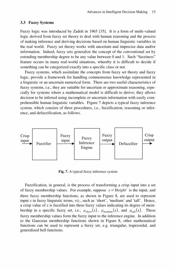
Fuzzy systems, which assimilate the concepts from fuzzy set theory and fuzzy logic, provide a framework for handling commonsense knowledge represented in a linguistic or an uncertain numerical form. There are two useful characteristics of fuzzy systems, i.e., they are suitable for uncertain or approximate reasoning, espe-cially for systems where a mathematical model is difficult to derive; they allows decision to be inferred using incomplete or uncertain information with easily com-prehensible human linguistic variables. Figure 7 depicts a typical fuzzy inference system, which consists of three procedures, i.e., fuzzification, reasoning or infer-ence, and defuzzification, as follows.
Fig. 7. A typical fuzzy inference system
Fuzzification, in general, is the process of transforming a crisp input into a set of fuzzy membership values. For example, suppose '' Heightx = is the input, and
three fuzzy membership functions, as shown in Figure 8, are used to represent input x in fuzzy linguistic terms, viz., such as ‘short’, ‘medium’ and ‘tall’. Hence, a crisp value of x is fuzzified into three fuzzy values indicating its degree of mem-bership in a specific fuzzy set, i.e., ( )xμshort , ( )xμmedium , and ( )xμtall . These
fuzzy membership values form the fuzzy input to the inference engine. In addition to the Gaussian membership functions shown in Figure 8, other mathematical functions can be used to represent a fuzzy set, e.g. triangular, trapezoidal, and generalized bell functions.
Fuzzifier Fuzzy
Inference Engine
Defuzzifier
Crisp input
Fuzzy input
Fuzzy output
Crisp output

16 C.P. Lim and L.C. Jain
Fig. 8. Fuzzification to obtain fuzzy membership values
The fuzzy inference engine contains a series of IF-THEN type of fuzzy rules to convert the fuzzy input into fuzzy output. These fuzzy rules are solicited from domain experts, and are used to perform reasoning based on the fuzzy input. Each fuzzy rule consists of parts: an antecedent of the IF part and a consequent of the THEN part, as follows
GYFxFxFx is THEN is AND .... is AND is IF nn 2211
where xi and Y are the inputs and output, and, Fi and G are the input and output linguistic variables or fuzzy sets respectively. If the antecedent of a given rule has more than one part, a process known as implication is conducted. Fuzzy opera-tors, such as AND or OR, can be applied to obtain a representative result of the antecedent for that rule. Several methods can be used to perform inference with the AND or OR operator. For example, the traditional Mamdani fuzzy inference system [36] treats AND and OR as the “min” and “max” functions, respectively. The representative result is then applied to the rule consequent, i.e., an output linguistic variable represented by a fuzzy membership function. This implication process is applied to each rule. Since a series of rules is available, an aggregation process to combine all the rule consequents is needed. By aggregation, the fuzzy sets that represent the outputs of each rule are combined into a single fuzzy set. Again, several aggregate operators, e.g. “max” or “sum”, are available to perform aggregation.
Defuzzification is the opposite process of fuzzification. It aims to obtain a rep-resentative value of the output fuzzy set, and to produce a crisp output. The centre of gravity is one of the most widely used defuzzification operators, which is simi-lar to the expected value of a probability distribution. Other defuzzification opera-tors, e.g. mean of maximum, bisector of area, the smallest of maximum, and the largest of maximum, are also available [36]. An example of the defuzzified crisp output is shown in Figure 9.
Antecedent Consequent

Advances in Intelligent Decision Making 17
Fig. 9. Defuzzification to produce a crisp output
3.4 Case Based Reasoning
Case based reasoning [37] is a branch of artificial intelligence founded on psycho-logical theory of human reasoning. Case based reasoning recognises that humans often solve a new problem by comparing it with similar ones that they had already resolved in the past [38]. Case based reasoning can be utilised as a decision sup-port approach in which previous similar solutions are retrieved and consulted to solve a new problem. A case based reasoning system draws its knowledge base from a reasonably large set of cases of past problems and solutions. The rationale of case based reasoning is that situations recur with regularity. What was done in one situation is likely to be applicable in a similar situation [39]. As shown in Figure 10, a typical case based reasoning cycle generally includes four basic pro-cedures, i.e., retrieval, reuse, and case revise, and retain [37].
A case based reasoning system consists of a case library, which is a repository of historical cases. Consider that a new problem (new case) is presented. Based on the new case, a search through the case library to find the historical cases that most closely resemble the new case is conducted. The comparison consists of matching attributes of the new case with those of each historical case, and comput-ing for each case a similarity metric. This metric provides an indication of how closely the new case matches each historical case. The most similar historical case is retrieved and is combined with the new case through the process of reuse to form a solved case, i.e., a proposed solution to the new case.
Through the revise process, the proposed solution is then evaluated for its cor-rectness, e.g. by comparing the solution with a supervisory signal or a confirmed target class. The proposed solution needs to be repaired should it fails to solve the new case satisfactorily. Once it is confirmed that the proposed solution works adequately, the retain process is initiated. The proposed solution is absorbed into
0
1 Membership function
Universe of discourse
Defuzzified crisp output

18 C.P. Lim and L.C. Jain
the case library as a new learned case or useful information from the proposed solution is integrated with some similar, existing case. The purpose is to continu-ally improve the case based reasoning system.
From Figure 10, it can be seen that general knowledge plays a role in the case based reasoning cycle. General knowledge is useful to supplement the informa-tion contained in historical cases. As a result, the proposed solution can be formu-lated in an accuracy manner not only based on the retrieved case but also from general domain-dependent knowledge.
Fig. 10. A typical case based reasoning cycle (source: [39])
New Case
New Case
Learned Case
Tested/ Repaired Case
Solved Case
Retrieved Case
Retrieve
Reuse
Revise
Retain
Previous Cases
General Knowledge
Confirmed Solution
Suggested Solution
Problem

Advances in Intelligent Decision Making 19
3.5 Agent-Based Systems
Agent-based systems are generally regarded as a distributed artificial intelligence paradigm. In [40], agents are described as “sophisticated computer programs that act autonomously on behalf of their users, across open distributed environments, to solve a growing number of complex problems”. This shows that agents are capable of making decisions and performing tasks autonomously. Indeed, intelli-gent agents are entities that are fixable to changing environments and changing goals. They learn from experience and make appropriate choices given perceptual limitations and finite computation [41].
Agents possess a variety of features. For instance, the essential versus empow-ering features of agents are described in [42]. The essential features of agents include goal orientation, persistence, and reactivity and interactivity. On the other hand, the empowering features of agents include artificial intelligence, mobility, and interactivity. As stated in [43], agent-based systems are empowered by their intelligence and ability to communicate with each other. Instead of one agent, an ensemble of agents can be deployed to form a multi-agent system. As shown in Figure 11, multi-agent systems sit in the quadrant with a high level of intelligence and a high degree of communication ability.
Fig. 11. Comparison of agent-based systems and other systems (Source: [43])
In multi-agent systems, a number of areas have been investigated. These in-
clude agent architecture, agent-system architecture, and agent infrastructure [44]. Studies in agent architecture focus on internal architectures of agents, such as components for perception, reasoning, and action. In agent-system architecture, agents’ interactions and organizational architectures are analysed, whereby agents operate and interact under specified environmental constrains. In agent infrastruc-ture, the interface mechanisms of multi-agent systems, which is mainly the com-munication aspect between agents are studied [45].
Intelligence
Communication
Multi-Agent Systems
Distributed Systems
Expert Systems
Conventional Systems

20 C.P. Lim and L.C. Jain
To perform a particular task, the relationship among a pool of agents in a multi-agent system needs to follow some pre-defined model. One of the earliest models is the Beliefs, Desires, Intentions reasoning model [46]. In this model, beliefs represent the agent’s understanding of the external world, such as information obtained from the surrounding environment; desires are the goals that the agent wants to achieve; and intentions are the plans the agent uses to reach its desires [47].
Another reasoning model is the trust-negotiation-communication model pro-posed in [48]. Figure 12 shows the types of interaction that are possible among agents. The model is based on the premise that the origin and the justification of the strength of beliefs comes from the sources of beliefs. In this model, four pos-sible sources of beliefs are considered: direct experience, categorization, reason-ing, and reputation [48].
Fig. 12. The trust-negotiation-communication model for multi-agent systems (Source: [48])
In the trust-communication-negotiation model, communication is concerned with the interaction among agents in order for them to understand each other. Negotiation, on the other hand, is concerned with how agent teams are formed. The core part of the model is basically on trust, whereby the main concern is how an agent handles trust and interacts with other agents. The questions raised in-clude ‘should an agent trust information given by another agent?’ or ‘should an agent trust another agent to perform a particular task?’ Indeed, the agents within the team collaborate with each other, and trust each other (inter-team relation).

Advances in Intelligent Decision Making 21
The model describes trust as a bond that can be strengthened via the exchange of certified tokens. In essence, trust is dynamic by nature. It is strengthened by successful interactions, and is weakened by unsuccessful outcomes. This model is useful for tackling various scenarios in complex decision making problems.
3.6 Remarks
A number of artificial intelligence techniques, i.e., artificial neural networks, evo-lutionary computing, fuzzy systems, case based reasoning, and agent-based systems, that can be applied to design and develop intelligent decision support systems has been briefly described. In addition to using each intelligent technique to solve real-world problems, more effective solutions can be obtained if they are used in combination. Indeed, hybrid paradigms combining two or more of intelli-gent techniques are becoming increasingly popular to deal with complex problems. Examples of hybrid paradigms include neural-fuzzy, neural-genetic, fuzzy-genetic, neural-fuzzy-genetic, fuzzy case based reasoning, evolutionary case based reasoning models, fuzzy agent-based systems, and multi-agent case based reasoning system, to name a few. Each combination brings synergy to the result-ing system in such a way that the hybrid paradigm exploits the advantages of the constituent techniques and, at the same time, avoids their shortcomings. Applica-tion examples are described in the next section.
4 Application Examples
In this section, application examples pertaining to intelligent techniques as well as hybrid intelligent techniques for undertaking decision making problems are pre-sented. Note that these application examples represent only a small sample of recent publications in the literature covering intelligent techniques as well as their hybrid paradigms with application to supporting human decision making proc-esses in various domains.
A backpropagation based neural network which attempts to model emotional factors in human learning and decision making is proposed in [49]. The emotional backpropagation network includes additional emotional weights that are updated using two emotional parameters, i.e., anxiety and confidence. The experimental results on a facial recognition problem show adding the emotional parameters is able to produce higher recognition rates and faster recognition time.
A hybrid known as Bayesian ARTMAP, which combines Fuzzy ARTMAP neural network and the Bayesian framework, is proposed in [50]. The Bayesian framework is used to improve classification accuracy and to reduce the number of category in Fuzzy ARTMAP. Based on synthetic and 20 real-world databases, it is demonstrated that Bayesian ARTMAP is able to outperform Fuzzy ARTMAP in terms of classification accuracy, sensitivity to statistical overlapping, learning curves, expected loss, and category proliferation.
In the medical area, decision support systems based on a decision tree, i.e., C4.5, and a backpropagation neural network to construct decision support systems for the prediction of regimen adequacy of vancomycin is reported in [51].

22 C.P. Lim and L.C. Jain
Bagging is also adopted to enhance the performance. The results show that the overall accuracy of C4.5-based or the neural network-based decision support sys-tem is better than that of the benchmark one-compartment pharmacokinetic model. On the other hand, a classifier-based ensemble system comprising neural net-works, support vector machines, Bayesian networks, and decision trees for sup-porting the diagnosis of cardiovascular disease based on aptamer chips is presented [52]. Again, the results demonstrate that the system is able to yield high diagnostic accuracy.
Sales forecasting is a challenging problem owing to the volatility of demand. A novel neural network known as the extreme learning machine to investigate the relationship between sales amount and significant factors that affect the demand is developed [53]. By using real data from a fashion retailer in Hong Kong, it is demonstrated that the proposed model is able to outperform backpropagation neu-ral network on several sales forecasting tasks.
A multiobjective evolutionary algorithm for groundwater management that op-timizes the placement and the operation of pumping facilities over time is ex-plained in [54]. Using a three-region problem, the algorithm is useful in assisting the investigation into the cost tradeoffs between different regions by providing an approximation to the Pareto-optimal set.
Another evolutionary computing model that applies two local search operators and Tabu Search for handling inventory routing problem is proposed in [55]. Two main components of the supply chain, i.e., transportation logistics and inventory control, are examined. The local search operators are used for dealing with the inventory and routing aspects of the problem, while Tabu Search for further reduc-ing the transportation costs. Satisfactory results both in terms of effectiveness and robustness are reported.
An evolutionary algorithm coupled with the expectation-maximization tech-nique to formulate Bayesian networks based on incomplete databases is suggested in [56]. A real-world data set related to direct marketing, i.e., predicting potential buyers from buying records of previous customers, is applied to evaluate the ap-plicability of the proposed system. The results demonstrate that the proposed system is able to outperform other methods in the presence of missing values.
Economic dispatch is a highly constrained optimization problem which in-volves interaction among decision variables. A fuzzy clustering-based particle swarm optimization system to undertake electrical power dispatch problems is described in [57]. The performance of the proposed system is examined using the standard IEEE 30 bus six-generator test system. High-quality solutions are pro-duced by the proposed system.
Multiple attribute decision analysis problems involve both quantitative and qualitative attributes with uncertainties, e.g. incompleteness (or ignorance) and vagueness (or fuzziness). To tackle this issue, a fuzzy interval grade evidential reasoning model is proposed in [58]. Local ignorance and grade fuzziness are modelled using a distributed fuzzy belief structure, leading to a fuzzy belief deci-sion matrix. Efficacy and applicability of the proposed model are illustrated with a numerical example.

Advances in Intelligent Decision Making 23
A method for pruning decision alternatives in ordered weighted averaging op-erators is suggested [59]. Inferior alternatives that are less competitive among competing alternatives in the ordered weighted averaging aggregation process are identified and eliminated. Efficacy of the proposed method is demonstrated using simulated decision problems of diverse sizes. The results show that the number of alternatives can be reduced drastically by applying the proposed method.
In [60], the capabilities of hierarchical fuzzy systems to approximate functions in discrete input spaces are examined. Useful properties pertaining to hierarchical fuzzy systems for function approximation and the associated accuracy of ap-proximation are discussed. A hierarchical fuzzy system identification method that combines human knowledge and numerical data for system construction and iden-tification is proposed. Applicability of the proposed method to site selection deci-sion support, i.e., a strategic decision making problem faced by many retail and service firms, is demonstrated. Based on some real commercial data, the proposed method outperforms regression and neural network approaches.
An inventory classification system based on the fuzzy analytic hierarchy proc-ess is described in [61]. Fuzzy concepts are integrated with real inventory data, and a decision support system that is useful for multi-criteria inventory classifica-tion is developed. The effectiveness of the proposed method is demonstrated using a study conducted in an electrical appliances company. On the other hand, a hybrid model combining fuzzy similarity measurement and fuzzy multi-criteria decision making for case based design under fuzzy environment is proposed in [62]. The advantages of using fuzzy sets include increasing the chance of good match, avoiding ‘‘too few” retrieved cases, and allowing situations with linguistic description to be handled. The proposed method is applied to power transformer concurrent design, and more suitable solutions, as compared with those from the similarity measurement only retrieval method, are produced.
A revised case based reasoning model to undertake decision making problems in project management is described in [63]. A new problem description approach, i.e., hierarchical criteria architecture, is proposed to enhance traditional case based reasoning technique, and a recommender system for software project planning, which is based on multiple objective decision and knowledge mining techniques, is implemented. Experiments using 41 real projects from a software consultancy firm demonstrate that the revised case based reasoning model is effective for pro-ject managers in planning and analysing project management activities.
Based on hybrid case-based reasoning and rule-based reasoning techniques, a clinical decision support system for ICU is constructed [64]. Case based reason-ing is able to supplement the difficulties in acquiring explicit knowledge for build-ing rule-based systems. The proposed hybrid model is able to provide clinical decision support for all domains of ICU. Efficacy of the proposed model is dem-onstrated using real ICU data as well as simulated data.
A generic case based reasoning system for helping safety managers to make decisions on prevention measures is described in [65]. The system makes recom-mendation based on similar past incidents and expertise driven advice. The system is tested using a real accident database from the marine industry, and the usefulness of the system is demonstrated.

24 C.P. Lim and L.C. Jain
A decision-making tool, developed based on a multi-agent system, for analys-ing and understanding dynamic price changes in the wholesale power market is described in [66]. The system is able to create a framework for assessing new trading strategies in a competitive electricity trading environment. Capabilities of the proposed system in terms of estimation, transmission, decision making, analy-sis, and intelligence are compared with those of other electricity trading software. The proposed system also exhibits better estimation accuracy as compared with those of neural network and genetic algorithm. A study using a data set pertaining to the California electricity crisis is conducted, and the results confirm the validity of the system.
In [67], an approach to incorporating Bayesian learning into a multi-agent sys-tem is described. A study to demonstrate that the system learns to identify an appropriate agent to answer free-text queries and keyword searches for defence contracting is conducted. The efficacy of the proposed system is determined by analysing the accuracy and degree of learning in the system. The system is tested against known, historical data, and the outcomes demonstrate that Bayesian learn-ing is a meaningful approach, and that learning does occur in the multi-agent system.
The role of automated agents for decision support in the electronic marketplace has attracted a lot of attention. As such, the efficacy of using automated agents for learning bidding strategies involving multiple sellers in reverse auctions is studied in [68]. It is argued that agents should be able to learn the optimal or best re-sponse strategies when they exist (rational behaviour) and should demonstrate low variance in profits (convergence). The desirable properties of rational behaviour and convergence are demonstrated using evolutionary and reinforcement learning agents.
A multi-agent based decision support system to help individuals and groups consider ethical perspectives in the performance of their tasks is described in [69]. Four distinct roles for ethical problem solving support, viz. advisor, group facilita-tor, interaction coach, and forecaster, are described. The belief-desire-intention model in agent technology is utilized as a method to support user interaction, simulate problem solving, and predict future outcomes.
The design and application of a multi-agent system for tackling a manufactur-ing problem, i.e., production scheduling, is presented in [70]. A coordination scheme for a multi-agent system is proposed, and its efficacy is tested against an existing framework of multi-agent learning without coordination. The agents in the manufacturing shop floor act as dispatchers to dispatch jobs over a machine. A knowledge base of dispatching rules and a genetic algorithm that learns new dis-patching rules over time are embedded into the agents. The results show that a multi-agent system where agents coordinate their actions performs better than one that agents do not coordinate their actions.
5 Summary
An overview of intelligent decision making is presented in this chapter. The proc-ess of human decision making and elements associated with decision quality are

Advances in Intelligent Decision Making 25
discussed. A taxonomy of decision support systems is also described. Techniques from artificial intelligence that are useful for the design and development of intel-ligent decision making models are also presented. These include artificial neural networks, evolutionary computing, fuzzy systems, case based reasoning, as well as multi-agent systems. Application examples that show how intelligent and hybrid intelligent techniques can be utilized to tackle decision making problems are high-lighted. It is envisaged that the general aspects of decision making, as well as the intelligent techniques and their associated application examples in a variety of domains as presented in this chapter serve as background for readers to better understand and comprehend chapters covered in this book.
References
[1] Holsapple, C.W.: Decisions and Knowledge. In: Burstein, F., Holsapple, C.W. (eds.) Handbooks on Decision Support Systems 1: Basic Theme, pp. 21–54. Springer, Hei-delberg (2008)
[2] Keen, P.G.W.: Decision Support Systems: An Organizational Perspective. Addison-Wesley Pub. Co., Reading (1978)
[3] González, J.R., Pelta, D.A., Masegosa, A.D.: A Framework for Developing Optimiza-tion-Based Decision Support Systems. Expert Systems with Applications 36, 4581–4588 (2009)
[4] Michalewicz, Z., Schmidt, M., Michalewicz, M., Chiriac, C.: Case Study: An Intelli-gent Decision-Support System. IEEE Intelligent Systems 20, 44–49 (2005)
[5] Guerlain, S., Brown, D.E., Mastrangelo, C.: Intelligent Decision Support Systems. In: Proceedings of IEEE International Conference on Systems, Man, and Cybernetics, vol. 3, pp. 1934–1938 (2000)
[6] Simon, H.: Administrative Behaviour, 4th edn. The Free Press (1997) [7] Borenstein, D.: Towards a Practical Method to Validate Decision Support Systems.
Decision Support Systems 23, 227–239 (1998) [8] Martinson, M., Davidson, R., Tse, D.: The Balanced Scorecard: A Foundation for the
Strategic Management of Information Systems. Decision Support Systems 25, 71–88 (1999)
[9] Forgionne, G.A.: Decision-Making Support System Effectiveness: The Process to Outcome Link. Information Knowledge Systems Management 2, 169–188 (2000)
[10] Phillips-Wren, G., Jain, L.C.: Recent Advances in Intelligent Decision Technologies. In: Apolloni, B., Howlett, R.J., Jain, L.C. (eds.) KES 2007, Part I. LNCS (LNAI), vol. 4692, pp. 567–571. Springer, Heidelberg (2008)
[11] Creswell, D.C., McNamee, P.C.: Decision Support, Decision Quality, and Strategic Decisions. In: Tonfoni, G., Jain, L. (eds.) Advanced Knowledge International Innova-tions in Decision Support Systems. International Series on Advanced Intelligence, vol. 3, pp. 1–16 (2003)
[12] Power, D.J.: Decision Support Systems: Concepts and Resources for Managers. Quo-rum Books, USA (2002)
[13] Power, D.J.: Specifying an Expanded Framework for Classifying and Describing De-cision Support Systems. Communications of the Association for Information Sys-tems 13, 158–166 (2004)

26 C.P. Lim and L.C. Jain
[14] McCulloch, W.S., Pitts, W.: A Logical Calculus of the Ideas Immanent in Nervous Activity. Bulletin of Mathematical Biophysics 5, 115–133 (1943)
[15] Rumelhart, D.E., Hinton, G.E., Williams, R.J.: Learning Internal Representation by Error Propagation. In: Rumelhart, D.E., McLelland, J.L. (eds.) Parallel distributed processing, vol. I, pp. 318–362. MIT Press, Cambridge (1986)
[16] Broomhead, D.S., Lowe, D.: Multivariate Functional Interpolation and Adaptive Networks. Complex Systems 2, 321–355 (1988)
[17] Kohonen, T.: Self-Organization and Associative Memory. Springer, Heidelberg (1984)
[18] Carpenter, G.A., Grossberg, S.: A Massively Parallel Architecture for a Self-Organizing Neural Pattern Recognition Machine. Computer Vision, Graphics and Im-age Processing 37, 54–115 (1987)
[19] Haykin, S.: Neural Networks: A Comprehensive Foundation. Macmillan, Basingstoke (1994)
[20] Grossberg, S.: Adaptive Pattern Classification and Universal Recoding I: Parallel De-velopment and Coding of Neural Feature Detectors. Biological Cybernetics 23, 121–134 (1976)
[21] Grossberg, S.: Adaptive Pattern Classification and Universal Recoding II: Feedback, Expectation, Olfaction, Illusion. Biological Cybernetics 23, 187–202 (1976)
[22] Grossberg, S.: How Does a Brain Build a Cognitive Code? Psychological Review 87, 1–51 (1980)
[23] Carpenter, G.A., Grossberg, S.: ART 2: Stable Self-Organization of Pattern Recogni-tion Codes for Analog Input Patterns. Applied Optics 26, 4919–4930 (1987)
[24] Carpenter, G.A., Grossberg, S.: ART 3 Hierarchical Search: Chemical Transmitters in Self-Organizing Pattern Recognition Architectures. Neural Networks 3, 129–152 (1990)
[25] Carpenter, G.A., Grossberg, S., Rosen, D.B.: Fuzzy ART: Fast Stable Learning and Categorization of Analog Patterns by An adaptive Resonance System. Neural Net-works 4, 759–771 (1991)
[26] Carpenter, G.A., Grossberg, S., Reynolds, J.H.: ARTMAP: Supervised Real-Time Learning and Classification of Nonstationary Data by a Self-Organizing Neural Net-work. Neural Networks 4, 565–588 (1991)
[27] Carpenter, G.A., Grossberg, S., Markuzon, N., Reynolds, J.H., Rosen, D.B.: Fuzzy ARTMAP: A Neural Network Architecture for Incremental Supervised Learning of Analog Multidimensional Maps. IEEE Transactions on Neural Networks 3, 698–712 (1992)
[28] Fogel, L.J., Owens, A.J., Walsh, M.J.: Artificial Intelligence Through Simulated Evo-lution. John Wiley, Chichester (1966)
[29] Rechenberg, I.: Evolutionary strategy. In: Zurada, J.M., Marks II, R.J., Robinson, C.J. (eds.) Computational Intelligence: Imitating Life, pp. 147–159. IEEE Press, Los Alamitos (1994)
[30] Koza, J.R.: Genetic Programming. The MIT Press, Cambridge (1992) [31] Holland, J.H.: Escaping Brittleness: The Possibility of General-Purpose Learning Al-
gorithms Applied to Parallel Rule-Based Systems. In: Michalski, R.S., Carbonell, J.G., Mitchell, T.M. (eds.) Machine Learning, vol. 2, pp. 593–624. Morgan Kauf-mann, San Francisco (1986)
[32] Holland, J.H.: Outline for a Logical Theory of Adaptive Systems. Journal of the ACM 3, 297–314 (1962)

Advances in Intelligent Decision Making 27
[33] Holland, J.H.: Adaptation in Natural and Artificial Systems. University of Michigan Press, Ann Arbor (1975)
[34] Dumitrescu, D., Lazzerini, B., Jain, L.C., Dumitrescu, A.: Evolutionary Computation. CRC Press, Boca Raton (2000)
[35] Zadeh, L.A.: Fuzzy Sets. Information and Control 8, 338–353 (1965) [36] Jang, J.S.R., Sun, C.T., Mizutani, E.: Neural-Fuzzy and soft Computing. Prentice-
Hall, Englewood Cliffs (1997) [37] Aamodt, E.P.: Case-Based Reasoning: Foundational Issues, Methodolgical Varia-
tions, and System Approaches. AI Communications 7, 39–59 (1994) [38] Chua, D.K.H., Li, D.Z., Chan, W.T.: Case-Based Reasoning Approach in Bid Deci-
sion Making. Journal of Construction Engineering and Management 127, 35–45 (2001)
[39] Kolodner, J.: Improving Human Decision Making Through Case-Based Decision Aiding. AI Magazine 12, 52–68 (1991)
[40] Balogh, Z., Laclavik, M., Hluchy, L.: Multi Agent System for Negotiation and Deci-sion Support. In: Proceedings of the Fourth International Scientific Conference Elec-tronic Computers and Informatics, pp. 264–270 (2000)
[41] Poole, D., Mackworth, A., Goebel, R.: Computational Intelligence: A Logical Ap-proach. Oxford University Press, Oxford (1998)
[42] Hess, T.J., Rees, L.P., Rakes, T.R.: Using Autonomous Software Agents to Create Next Generation of Decision Support Systems. Decision Sciences 31, 1–31 (2000)
[43] Ivancevic, V.G., Ivancevic, T.T.: Computational Mind: A Complex Dynamics Per-spective. Springer, Heidelberg (2007)
[44] Ferber, J.: Multi-Agent Systems: An Introduction to Distributed Artificial Intelli-gence. Addison-Wesley, Reading (1999)
[45] Dagli, C., Kilicay, N.: Understanding Behavior of System of Systems through Com-putational Intelligence Techniques. In: Proceedings of the First Annual IEEE Systems Conference, pp. 1–7 (2007)
[46] Bratman, M.E.: Intention, Plans, and Practical Reason. Harvard University Press, Cambridge (1987)
[47] Rao, A.S., Georgeff, M.P.: BDI Agents: From Theory to Practice. In: Proceedings of the First International Conference on Multiagent Systems, pp. 312–319 (1995)
[48] Haider, K., Tweedale, J., Urlings, P., Jain, L.: Intelligent Decision Support System in Defense Maintenance Methodologies. In: Proceedings of the International Conference on Emerging Technologies, pp. 560–567 (2006)
[49] Khashman, A.: A Modified Backpropagation Learning Algorithm With Added Emo-tional Coefficients. IEEE Transactions on Neural Networks 19, 1896–1909 (2008)
[50] Vigdor, B., Lerner, B.: The Bayesian ARTMAP. IEEE Transactions on Neural Net-works 18, 1628–1644 (2007)
[51] Hua, P.J.H., Wei, C.P., Cheng, T.H., Chen, J.X.: Predicting Adequacy of Vancomy-cin Regimens: A Learning-Based Classification Approach to Improving Clinical De-cision Making. Decision Support Systems 43, 1226–1241 (2007)
[52] Eom, J.H., Kim, S.K., Zhang, B.T.: AptaCDSS-E: A Classifier Ensemble-Based Clinical Decision Support System for Cardiovascular Disease Level Prediction. Ex-pert Systems with Applications 34, 2465–2479 (2008)
[53] Sun, Z.L., Choi, T.M., Au, K.F., Yu, Y.: Sales Forecasting Using Extreme Learning Machine with Applications in Fashion Retailing. Decision Support Systems 46, 411–419 (2008)

28 C.P. Lim and L.C. Jain
[54] Siegfried, T., Bleuler, S., Laumanns, M., Zitzler, E., Kinzelbach, W.: Multiobjective Groundwater Management Using Evolutionary Algorithms. IEEE Transactions on Evolutionary Computation 13, 229–242 (2009)
[55] Zachariadis, E.E., Tarantilis, C.D., Kiranoudis, C.T.: An Integrated Local Search Method for Inventory and Routing Decisions. Expert Systems with Applications 36, 10239–10248 (2009)
[56] Wong, M.L., Guo, Y.Y.: Learning Bayesian Networks from Incomplete Databases Using a Novel Evolutionary Algorithm. Decision Support Systems 45, 368–383 (2008)
[57] Agrawal, S., Panigrahi, B.K., Tiwari, M.K.: Multiobjective Particle Swarm Algorithm With Fuzzy Clustering for Electrical Power Dispatch. IEEE Transactions on Evolu-tionary Computation 12, 529–541 (2008)
[58] Guo, M., Yang, J.B., Chin, K.S., Wang, H.W., Liu, X.B.: Evidential Reasoning Ap-proach for Multiattribute Decision Analysis Under Both Fuzzy and Interval Uncer-tainty. IEEE Transactions on Fuzzy Systems 17, 683–697 (2009)
[59] Ahn, B.S., Park, H.: An Efficient Pruning Method for Decision Alternatives of OWA Operators. IEEE Transactions on Fuzzy Systems 16, 1542–1549 (2008)
[60] Zeng, X.J., Goulermas, J.Y., Liatsis, P., Wang, D., Keane, J.A.: Hierarchical Fuzzy Systems for Function Approximation on Discrete Input Spaces With Application. IEEE Transactions on Fuzzy Systems 16, 1197–1215 (2008)
[61] Cakir, O., Canbolat, M.S.: A Web-Based Decision Support System for Multi-Criteria Inventory Classification Using Fuzzy AHP Methodology. Expert Systems with Ap-plications 35, 1367–1378 (2008)
[62] Qi, J., Hu, J., Peng, Y.H., Wang, W., Zhang, Z.: A Case Retrieval Method Combined with Similarity Measurement and Multi-Criteria Decision Making for Concurrent De-sign. Expert Systems with Applications 36, 10357–10366 (2009)
[63] Yang, H.L., Wang, C.S.: Recommender System for Software Project Planning One Application of Revised CBR Algorithm. Expert Systems with Applications 36, 8938–8945 (2009)
[64] Kumar, K.A., Singh, Y., Sanyal, S.: Hybrid Approach Using Case-Based Reasoning and Rule-Based Reasoning for Domain Independent Clinical Decision Support in ICU. Expert Systems with Applications 36, 65–71 (2009)
[65] Virkki-Hatakka, T., Reniers, G.L.L.: A Case-Based Reasoning Safety Decision-Support Tool: Nextcase/Safety. Expert Systems with Applications 36, 10374–10380 (2009)
[66] Sueyoshi, T., Tadiparthi, G.R.: An Agent-Based Decision Support System for Whole-sale Electricity Market. Decision Support Systems 44, 425–446 (2008)
[67] Montano, B.R., Yoon, V., Drummey, K., Liebowitz, J.: Agent Learning in the Multi-Agent Contracting System [MACS]. Decision Support Systems 45, 140–149 (2008)
[68] Sikora, R.T., Sachdev, V.: Learning Bidding Strategies with Autonomous Agents in Environments with Unstable Equilibrium. Decision Support Systems 46, 101–114 (2008)
[69] Robbins, R.W., Wallace, W.A.: Decision Support for Ethical Problem Solving: A Multi-Agent Approach. Decision Support Systems 43, 1571–1587 (2007)
[70] Pendharkar, P.C.: The Theory and Experiments of Designing Cooperative Intelligent Systems. Decision Support Systems 43, 1014–1030 (2007)

L.C. Jain and C.P. Lim (Eds.): Handbook on Decision Making, ISRL 4, pp. 29–53. springerlink.com © Springer-Verlag Berlin Heidelberg 2010
Chapter 2
IDSSE-M: Intelligent Decision Support Systems Engineering Methodology
M. Mora1, G. Forgionne2, F. Cervantes-Pérez3, and O. Gelman4
1 Department of Information Systems, Autonomous University of Aguascalientes, Aguascalientes, Mexico, 20000 [email protected]
2 Department of Information Systems, University of Maryland Baltimore County, Catonsville, MD 21250 USA [email protected]
3 CCADET, Universidad Nacional Autónoma de México (UNAM), Mexico, D.F. 04510 [email protected]
4 CCADET, Universidad Nacional Autónoma de México (UNAM), Mexico, D.F. 04510 [email protected]
Abstract. This chapter describes and illustrates IDSSE-M, a methodology for designing and building intelligent decision support systems. IDSSE-M follows a prototype-based evolutive approach on four main phases: project initiation, system design, system building and evaluation, and user’s definitive acceptance. IDSSE-M is theoretically founded in Saxena’s Decision Support Engineering Methodology, and Turban and Aronson’s DSS Building Paradigm. Although IDSSE-M has been only used in academic settings), the complexity of the implementations has been high, and based on realistic organizational cases, with satisfactory results. Main benefit of IDSSE-M is providing a systematic software engineering oriented process for new developers of intelligent DMSS.
1 Introduction
Decision-making Support Systems (DMSS) (Forgionne et al, 2005) – also named Management Support Systems (MSS) (Turban and Aronson, 1998) - are Information Systems (IS) designed specially to support some, several or all phases of an individual, team, organizational or intra-organizational decision-making process. From its origin in the early 1970s (Scott Morton, 1971) until now (McCosh and Correa-Perez, 2006), successful implementations of DMSS have been demanded mainly by large organizations due to the relevance of the benefits expected. Table 1 presents reported benefits and demands for four types of DMSS.
In spite of the reported interest, it has been widely documented that achieving a successful implementation of a DMSS is a complex task (Mora et al, 2003). However, there is not a standard framework or taxonomy of factors related to the success of a DMSS implementation. Updated from Mora et al (2003) five schemes

30 M. Mora et al.
Table 1. Main Reasons for Using DMSS
Purposes and Needs for using Model-Based DSS
Purposes and Needs for using Executive-Based DSS
• Improve the quality of decisions. • Increase productivity of analysts. • Facilitate communication between
decision makers and analysts. • Save analysis time. • Support objective-based decisions. • Reduce costs derived from wrong
decisions. • Incorporate decision-makers insights
and judgments into analysis.
• Increased competition. • A highly dynamic business
environment. • Need of a fast executive response. • Need of timely executive information. • Need of improved communications • Need of rapid status on operational data. • Scan the external decision environment. • Capture, filter, and focus on external
and internal data. Purposes and Needs for using
Knowledge-Based DSS Purposes and Needs for using
General-Based DSS • Preserve valuable and scarce
knowledge. • Share valuable and scarce knowledge. • Enhance problem solving abilities of
users. • Develop user’s job skills. • Increase productivity. • Improve quality of solution provided. • Guide the user through the problem
solving process. • Provide explanations for
recommended actions.
• Improve some or several phases of an individual, team or organizational decision-making process.
• Increase the probabilities of better outcomes of a decision-making process.
• Improve the decision makers’ shared-vision of the organization
• Seek efficiency and effectiveness of top decision makers regarding decision tasks.
• Explore consequences of critical decisions before they are taken and implemented.
have been identified -and exhibited in Table 2-: (i) a framework for the implementation of executive-based DSS (Watson et al, 1991); (ii) a framework of model-based DSS (Eierman et al, 1995), (iii) a framework for knowledge-based DSS derived from several sources; (iv) a framework for integrated DMSS (Mora et al, 2003) and (v) a framework of successful factors under a qualitative rationality derived from frameworks (i)-(iv).
In Table 2, each symbol means that the factor has been found in most studies reviewed by the framework’s authors. The set of eight categories are derived from Mora et al’s framework (2003) and suggests that a DMSS implementation process must consider at least one factor from each category to have a more comprehensive account of the phenomenon. Factor categories are: user, task, development team, process, technology, organization, environment and the system. Table 2’s final column then is generated for a general DSS or DMSS, under a qualitative and linear rationality that suggests the factors to be positively tested.
With the evidence reported from the several frameworks, the most likely successful factors for each category are respectively: user aptitude toward the DMSS, alignment or priority of the decisional task to be supported by the DMSS, the existence of a project champion for the DMSS project, the support provided by

IDSSE-M: Intelligent Decision Support Systems Engineering Methodology 31
the IS area of the organization to the DMSS project, a suitable development methodology, adequate software and hardware technology for building and deploying the DMSS, the existence of positive top management support, sponsor and organizational climate, an uncertain business environment, the easein utilizing the DMSS, and the timely delivery of the provided information. In turn, elements from Table 2, with few symbols indicate that such sampled populations of DMSS projects were found not statistically meaningful.
Table 2. Main List of Factors for Successful and Failed DMSS Implementations
Categories of Factors and Single Factors
Mora et al’s Scheme
Eierman et al’s
Scheme
Watson et al’s
Scheme
Several Sources
Most Likely Evidence to be
tested
DSS
EIS
ES
Model-based DSS
Executive-
based DSS
Knowledge-based DSS
General DSS or DMSS
1. User characteristics x x x ● ● ● ●●●●● User aptitude ✔ ✔ ✔ ● ◗ ●●●● Norm motivation ✔ ✔ ● ●●● Cognitive style ✔ ● Realistic expectations. ✔ ● ◗ ●●◗ 2. Task characteristics
x x x ● ◗ ●●●●
Task difficulty and newness
✔ ◗ ◗◗
Task uncertainty degree
✔ ◗ ◗◗
Task organizational alignment (priority)
✔ ✔ ◗ ◗ ◗◗◗
Adequate task domain and complexity
✔ ● ◗ ◗◗
3. Development team characteristics
x x x ● ◗ ◗◗◗
Project champion ✔ ✔ ✔ ◗ ◗◗◗ Leader’s business skills
✔ ◗
Leader’s technical skills
✔ ◗
Developers’ technical skills.
✔ ● ◗◗
4. Process characteristics
x x x ● ● ● ◗◗◗◗◗
User training. ✔ ● ● ◗ ◗◗◗ User involvement. ✔ ● ● ◗◗ Development Methodology (Evolved)
✔ ✔ ✔ ● ◗ ● ◗◗◗◗◗
Development frame time
✔ ◗ ◗◗
Cost-benefit analysis ✔ ✔ ● ◗ ◗◗◗◗ Data accessibility ✔ ● ◗◗

32 M. Mora et al.
Table 2. (continued)
Categories of Factors and Single Factors
Mora et al’s Scheme
Eierman et al’s
Scheme
Watson et al’s
Scheme
Several Sources
Most Likely Evidence to be
tested
DSS
EIS
ES
Model-based DSS
Executive-
based DSS
Knowledge-based DSS
General DSS or DMSS
Change and resistance management
✔ ✔ ● ◗◗◗
Support for evolution and diffusion
✔ ● ◗ ◗◗◗
Support of IS department
✔ ✔ ● ● ● ◗◗◗◗◗
Commitment of maintenance
✔ ◗ ◗◗
5. Technological characteristics
x x x ● ● ● ◗◗◗◗◗
Adequate Software ✔ ✔ ✔ ● ● ◗ ◗◗◗◗◗ Adequate Hardware ✔ ✔ ✔ ● ● ◗ ◗◗◗◗◗ 6. Organizational characteristics.
x x x ◗ ● ● ◗◗◗◗◗
Top management support
✔ ✔ ✔ ● ◗ ● ◗◗◗◗◗
Top sponsor ✔ ✔ ● ● ◗ ◗◗◗◗ Organizational climate ✔ ◗ ● ◗◗◗ 7. Environment characteristics.
x x x ● ● ● ◗◗◗◗◗
Hostile and uncertainty environment
✔ ● ◗ ◗ ◗◗◗◗
Relations with IT suppliers and IT research centers
✔ ● ◗◗
8. System (DMSS) characteristics.
x x x ● ● ● ◗◗◗◗◗
Accuracy and format of results
✔ ✔ ● ◗◗
Management level supported
✔ ● ◗◗
Decisional phase supported
✔ ● ◗◗
Relevance of results ✔ ● ◗◗ Degree of system sophistication
✔ ● ◗◗
Timeless information ✔ ● ◗ ◗◗◗ Easiness of usage ✔ ◗ ◗ ◗◗◗ Impact in user’s work ✔ ◗ ◗◗ Legal & ethical issues ✔ ● ◗◗

IDSSE-M: Intelligent Decision Support Systems Engineering Methodology 33
As Table 2 exhibits –generated from Mora et al (2003) –there are multiple factors that could prevent a successful DMSS implementation. In this chapter, we are interested in the factors related with development methodology and technical H/S issues. In particular, we claim that a well-defined hybrid-integrated or agile well agreed systems development methodologies can promote implementation success (Mahmood and Medewitz, 1985).
This chapter describes and illustrates IDSSE-M, a methodology for designing and building intelligent decision support systems. IDSSE-M is founded on a prototype-based evolutive approach involving four main phases: project initiation, system design, system building and evaluation, and user’s definitive acceptance. From the several available DMSS methodologies (Gachet and Haettenschwiler, 2006), IDSSE-M integrates activities from Saxena’s Decision Support Engineering Methodology (1991) and Turban and Aronson’s DSS Building Approach (1998). We report that IDSSE-M has been only used in academic settings (in six MSc courses on DMSS from 2000 to 2008 year, and two MSc theses (Lopez, 2007; Calderon, 2007)). However, the complexity of the prototype scholarly projects has been high and based on realistic organizational cases, and IDSSE-M has produced initial satisfactory results. In particular, the main benefit of IDSSE-M is to provide a systematic software engineering oriented process for new developers of intelligent DMSS.
The remainder of this chapter continues as follows: in section 2, a general review of DMSS methodologies is reported. In section 3, IDSSE-M is described. In section 4, a demo case for illustration purposes and empirical exploratory evaluations are reported. The chapter concludes with recommendations and limitations.
2 An Overview of DMSS Methodologies
Several methodologies for developing DMSS (DSS, EIS and KBS) have been posited (Gachet and Haettenschwiler, 2005). These methodologies can be grouped by type of development paradigm: traditional, iterative (prototyping/evolutive or adaptive), and a hybrid-integrated approach. While the literature (Alavi and Nappier, 1984; Mahmood and Medewitz, 1985) reports that traditional/classic SDLCs are not suggested for DMSS, given the lack of well-defined requirements in advance from users and the semi-structuredness of the decision-making situation, the first DMSS were developed through a classic SDLC (Turban and Aronson, 1998). Advances in DSS methods and foundations have have had a positive impact in overcoming earlier difficulties reported in the literature. Furthermore, while DMSS have special characteristics (decision-making purpose, intensive in a model-based design, with high strategic impact, and used by top and middle level users), they are also systems that must be planned, designed and built, through a systematic process (either traditional, iterative or hybrid-integrated).
In their comprehensive DMSS development methodologies’ study, Gachet and Haettenschwiler (2005) report “… nevertheless, the SDLC remains useful as a reference model and as an idealized abstraction of a more realistic DSS development process”. Consequently, while iterative DMSS development approaches are preferred, there is evidence that supports a well-managed

34 M. Mora et al.
Table 3. DMSS Development Methodologies
MAIN FEATURES TYPE OF DEVELOPMENT
PARADIGM ADVANTAGES DISVANTAGES
Classic SDLC Paradigm: • Waterfall (Royce, 1970; Marakas,
1999)
• Strong project management support.
• Well-known development methodology.
• It can be customized.
• On complex decision-making problems, a prototyping phase will initially be required.
• It can be perceived as a “heavy” methodology.
• It provides useful results until its completion.
Iterative Paradigm: • Prototyping/Evolutive (Courbon et
al, 1980; (quoted in Turban and Aronson, 1998); Alavi and Henderson, 1981; Nauman and Jenkins, 1982; Alavi, 1984)
• Adaptive ( Keen, 1980)
• It delivers rapid and visible initial results to users.
• It can be iterated until final completion of the system.
• In large-scale and complex DMSS it can save valuable resources.
• In large-scale and complex DMSS it reduces design risks.
• It fosters user participation leading to more user satisfaction.
• It can cause a disordered process when it is badly managed.
• It can be instanced differently by the same team in the same organization producing variability of results.
• It can generate a final useful DMSS but not totally documented with high risks in required future improvements.
• It demands usually state of the art development tools.
Integrated Focus / Hybrid Paradigms:
• DSS Design Cycle (Keen and Morton, 1978; quoted in Gachet and Haettenschwiler, 2005)
• DSS Development Phases (Carlson, 1979)
• DSS Development Cycle (Meador et al, 1984)
• Decision Support Systems Engineering (Sage, 1981; 1991)
• Decision Support Engineering (Saxena, 1991)
• IDSSE-M (reported in this chapter)
• Ideally this approach must provide similar advantages of the previous approaches.
• Presents a dual-view approach where designers and users can adapt the methodology.
• Ideally this approach must reduce similar disadvantages of the previous approaches.
• It must be dominated to avoid methodological confusion on its application.

IDSSE-M: Intelligent Decision Support Systems Engineering Methodology 35
development process or a hybrid-integrated process for developing DMSS (Mahmood, 1987; Sage, 1981; 1991; Turban, 1992).
Table 3 reports the main DMSS development methodologies, as well as their positive and negative core features (a full comparative study beyond the scope of this chapter). In Table 3IDSSE-M (the methodology reported here) is classified as hybrid-integrated approach (e.g. an iterative well-defined development process).
Hence, the availability of DMSS methodologies reported in the scientific literature can be considered abundant. However, from a scholastic viewpoint, few full methodologies have been reported in DMSS textbooks. Saxena (1991, p. 98) for instance reports “ … unfortunately DSS development has very often been an innovative but ad hoc process. Concrete experience with the design and development of complex and/or large scale DSSs is still mostly limited to either research institutions or large corporations.” We consider that more detailed descriptions of DMSS methodologies must be reported. This chapter pursues this aim.
3 IDSSE-M
IDSSE-M is a methodology for designing and building intelligent decision support systems. An initial draft was developed in an internal research project at UAA, Mexico (Mora, 1998), and subsequent improvements are reported in this chapter. IDSSE-M follows a prototype-based evolutive approach with four main phases: project initiation, system design, system building and evaluation, and user’s definitive acceptance. IDSSE-M can be considered an adaptation from Saxena’s Decision Support Engineering Methodology and Turban and Aronson’s DSS Building Paradigm. Table 4 reports a map of IDSS-M phases with previous methodologies. Space limitations preclude an extensive analysis of this comparison but references will be used in the IDSSE-M description.
IDSSE-M is a prototype-based evolutive approach. Evolutive (also called iterative (Jalote, 1997)) implies that software is released in several iterations and where in each iteration, the release is a functional version. In a strict sense, prototyping (Ginac, 1998) does not deliver functional versions. In IDSSE-M, prototyping is used in phase 2, if a more realistic version of the system must be presented to users, and it is focused on the user interface (UI) design activity.
In the first phase (project initiation), the main purpose is the formalization and agreement of the development of an IDSS. Three activities are suggested: 1.1 recognition of a decision-making situation; 1.2 justification of an IDSS; and 1.3 building planning. Activity 1.1 is used for a quick but essential identification of a critical decision-making situation. It uses a schematic diagram (users, problem, expected goal, decision unit, and list of potential courses of action) for supporting a fast visualization of the main decision-making general elements. While a IDSS is assumed to support semi-structured decisions, it is also expected that users can help to delimit the general structure of the problem. This activity 1.1 accounts for Turban and Aronson’s (1998) activities 1.1, 1.2, 1.3, and 1.4, and partially Saxena’s (1991) activities 1.1, 2.1, 2.2 and 2.3. Activity 1.2 (project justification) is realized for identifying and estimation of the most potential tangible and intangible expected benefits from the IDSS. In activity 1.3 (building planning), the

36 M. Mora et al.
building approach is established (a new internal or external development from scratch, or via an already package), and the estimated plan and project team (user, IDSS analyst, and IDSS builder(s)) is identified. An iterative approach does not imply that a set of first iterations can be estimated in advance. It is required for delivering a full final version. It can be expanded in the future, but it would be through a new project. Both activities accounts for Turban and Aronson’s (1998) activities 2.1, and 2.2, and Saxena’s (1991) activity 1.2.
In the second phase (design), the main purpose is the analysis and detailed design of the IDSS. Five activities are realized: 2.1 design of IDSS general core elements; 2.2 design of IDSS architecture; 2.3 design of DSS detailed core elements; 2.4 impact of scenarios; and 2.5 design of numerical, symbolic, DB, UI, & process models. These activities account for Saxena’s (1991) full requirements engineering and system design phases and Turban and Aronson’s (1998) activity 2.3 and full design phase.
In activity 2.1 (general design), a diagram is used for identification of four core elements: decision variables (x1, x2, …); scenario variables (z1, z2, …); output variables (y1, y2, …); and parameters (w1, w2, …). In a complex IDSS, such variables can be grouped and several detailed diagrams can be depicted. In activity 2.2 (architecture design), five possible arrangements (internal structures) are suggested: a DSS-ES (decision support system – expert system), a ES-DSS, a DSS with an included ES, an ES with an included DSS, a general system that controls at least one DSS and one ES. A final diagram of architecture is realized where its internal structure and its decision, scenario, output, and parameters variables are reported. In activity 2.3 (detailed design), a dictionary of elements for the four set of core elements (x’s, z’s, y’s, and w’s) is generated. In the dictionary of elements the following data by each element are reported: code identification, name, value (range of numerical or qualitative values), source (user data, numerical model, or qualitative model), and comments. Hence, no explicit numerical or qualitative model is developed. This approach is top-down (from black to white box) that manages design complexity from high to low abstraction design layers. In activity 2.4 (impact of scenarios) through influence diagrams, are introduced the next design level. First, models are developed that relate the four set of variables, and the probabilistic and inferential relationships between the variables are estimated. Conditional matrixes with probability ranges and expected outputs must be generated.
In activity 2.5 the specific numerical and inference (symbolic) procedures must be defined, as well as the detailed design of data, user interface and process-module models. Numerical models are reported in the classic format (inputs, algorithm, outputs), and symbolic relationships are specified through decision tables. The data model is reported through a classic entity-relationship diagram and complemented with a detailed design of tables. User interface (UI) design is reported through a navigation map plus the detailed design of each screen. Finally, process-module design refers to the physical architecture of the IDSS (a classic diagram 0 or a component diagram can be used).
In the third phase (building and evaluation) three activities are realized: 3.1 construction & model integration; 3.2 test case planning; and 3.3 user’s evaluation. This phase accounts for Saxena’s (1991) prototyping phase and 6.1 activity (user evaluation), and for Turban and Aronson’s (1998) construction and

IDSSE-M: Intelligent Decision Support Systems Engineering Methodology 37
implementation phases. In the 3.1 activity, software tools are selected, and there is a codification and/or assembling of pre-packaged modules, and the modules are fully integrated. In activity 3.2, test cases are readied for internal (done by developers) and external (cases prepared by users) validation. Finally, in activity 3.3, a definitive evaluation from users is realized. Critical decisions must be made: (i) close project with current version, (ii) authorize minor changes and end it, or (iii) authorize next iteration (with additional significant additions). If course of action (i) is decided, then the final phase (project ending) must be realized. Otherwise, an update of documentation is prepared.
Table 4. A Map of I-DSSE-M Methodology and Core Methodological Roots
IDSSE-M Saxena’s DSE Turban & Aronson’s DSS Building Phases
1. IDSS Project Initiation Phase.
1. Problem Definition and Feasibility Assessment Phase.
1. Planning Phase.
1.1 Problem assessment (size, complexity, and structuredness classification).
1.2 Feasibility study (technical, economic and operational).
1.1 Problem Identification. 1.2 Objectives of DSS. 1.3 Key decisions
supported. 1.4 Documental research.
2. Decision Task Analysis Phase.
2. Analysis Phase.
1.1 Recognition of a decision-making situation.
1.2 Justification of a IDSS. 1.3 Building planning.
2.1 Set decision scenarios. 2.2 Identification of
decision objects. 2.3 Task structure
modeling.
2.1 Construction strategy selection.
2.2 Resources identification.
2.3 Conceptual design. 2. IDSS Design Phase. 3. Requirements
Engineering Phase. 3. Design Phase.
3.1 User analysis. 3.2 Functional and
decisional analysis. 3.3 Data & knowledge
analysis. 3.4 User interface analysis. 3.5 H&S environment
selection. 3.6 Usability analysis. 4. Systems Design Phase.
2.1 IDSS general core elements.
2.2 IDSS architecture. 2.3 IDSS detailed core
elements. 2.4 Impact of scenarios. 2.5 Numerical, symbolic,
DB, UI, & process-module models.
4.1 DSS architecture design.4.2 UI Design. 4.3 Model design. 4.5 DB design. 4.5 Knowledge design.
3.1 UI Design. 3.2 Model design. 3.3 DB design. 3.4 Knowledge design.

38 M. Mora et al.
Table 4. (continued)
IDSSE-M Saxena’s DSE Turban & Aronson’s DSS Building Phases
3. IDSS Building & Evaluation.
5. Prototyping Phase. 4. Construction Phase.
4.1 DSS Programming. 5. Implementation
Phase.
3.1 Construction & model integration.
3.2 Test case planning. 3.3 User’s evaluation.
5.1 DSS building.
5.1 Testing, evaluation & demonstration.
5.2 Training & deployment.
4. IDSS Project Ending. 6. User Evaluation and
Adaptation Phase. 6. Maintenance &
Evolution Phase. 4.1 Documentation. 4.2 Training (if required). 4.3 Closure project.
6.1 User evaluation. 6.2 Adaptation process.
6.1 Ongoing support. 6.2 Evolution through
earlier steps.
The fourth phase is expected to be realized after several iterations. Saxena’s (1991) and Turban and Aronson’s methodologies do not report this phase explicitly (1998). IDSSE-M supports the project management view of the relevance of formal start and closure. Three activities are suggested: 4.1complete full documentation; 4.2 conduct training (if required); and 4.3formally to close the project. Best practices of system development (any paradigm) include the activity of documentation completion. Training is optional relying on the type of users (advanced and neophytes) and the complexity of the developed system. A formal ending of the project is useful to clarify the achievements and correct utilization of economic and human resources invested in the project, and for separating the potential new additions as a new project (and with a new demand of resources).
We believe that IDSSE-M is a methodology that provides an ordered development structure for guiding the design of simple and complex intelligent decision support systems. The approach relies on similar core development process and activities reported in the literature (Saxena, 1991; Turban and Aronson, 1998).
4 IDSSE-M: Illustration
IDSSE-M has been used in academic settings in one short research project in 1998, six MSc courses on DMSS in a MSc on IT program during 2000, 2002, 2004, 2006, 2007, and 2008 by around 22 teams of graduate students, and for developing two MSc theses (Lopez, 2007; Calderon, 2007), all at the Autonomous University of Aguascalientes, Mexico. The lead author of this chapter is the main designer of IDSSE-M, and has been the instructor of the MSc courses, as well as the director of the two MSc theses. Co-authors have reviewed and suggested improvements for the methodology. While a numerical evaluation of several

IDSSE-M: Intelligent Decision Support Systems Engineering Methodology 39
Fig. 1. Recognition of a decision-making general situation
usability constructs has been conducted, it will be reported in a subsequent article. Here, we can report that qualitative comments from teams during the presentation of their final term projects have been positive. It is relevant to report also that the complexity of the prototype scholarly projects has been high and based on realistic organizational cases.
The main benefit of IDSSE-M is providing a systematic software engineering oriented process for new developers of intelligent DMSS. We illustrate its utilization with the demo case used for teaching purposes in the MSc course. Appendix A reports the general description of the case.
In the activity 1.1 (recognition of a decision-making situation) as part of the IDSS Project Initiation Phase, a scheme for capturing the general structure of the decision-making situation is realized. Figure 1 shows the used scheme. The main problem is the lack of financial models that help to support financial decisions on business strategy. Two identified main courses of action (and that are not known in advance which one is the best) are: (i) to keep the current business strategy or (ii) to implement a new strategy. All details of the potential consequences of the same or new strategy are developed in the next stages.
In activity 1.2 (justification of an IDSS) the main user (Mr. Smith) and IDSSE analyst must estimate tangible and intangible benefits. In this demo case, Mr. Smith is responsible to estimate the cost of decisional mistakes caused by wrong financial estimations, caused by the lack of financial models. In turn, the IDSSS analyst is responsible to estimate development costs. Once the estimates are provided, a cost analysis benefit can be realized. In 1.3 activity, the IDSSS analyst develops a development plan (activities, schedule, costs, and main deliverables). In a real case, negotiations can happen until a final agreed plan is achieved.
In the IDSSE design phase, several types of design elements are realized. The initial design model is the general structure for the IDSS. Figure 2 shows such a structure.

40 M. Mora et al.
Fig. 2. Core general IDSS structure and IDSS Architecture
Variables identified are: y1, y.2, and y.3 (the 7th year row of financial data for both balance and income statement sheets, financial ratios, and trends on y.1); x.1 (decision variable on main business strategy); z.1 and z.2 (economic variables and competitor’s strategy); and w.1, w.2, and w.3 (parameters of balance sheet, income statement sheet, and other financial data for the last six years). At this stage, no detailed formula is required but only the general structure of the IDSS. For this demo case, the complexity involves the difficulty to generate adequate financial models rather on the difficulty to design the general structure. However, we believe that the initial two diagrams (figures 1 and 2) can help on more complex decisional situations through the identification of the essential variables of: output, decision, scenario, and parametric. In Figure 2, the IDSS architecture is also reported The IDSS structure for this case does not exhibit the internal DSS and ES components, and the four outputs (y’s) are reported as final outputs. In the IDSS architecture, the design decision is that three outputs (y1, y.2, and y.3) are intermediate outputs, and the eventual output is y.4. In this case, the first arrangement (e.g. a DSS-ES order) is used.
Next, the design activity is the generation of a dictionary of elements. For each category of variables (decision, scenario, output, and parameter) a data entry is generated with the following items: id code, name, range of values, origin or source, and comments. Tables 5 and 6 reports partially some entries. For instance, in Table 5, a partial view of outputs y’s is reported (from y.3.1 to y.3.13): trends in financial ratios. Y.3.1 is the trend in the current ratio, with a qualitative range of values between decreasing, stable, or growing, that will be calculated by a numerical model NM.3, via a linear regression model, and finally converted to a qualitative value. In a similar way, in Table 6, w.1 is the code for the entry referred to as cash parameters for the last six years, and T.1 is the identification of the data table for their sourcing. Other entries in both tables reports similar information.

IDSSE-M: Intelligent Decision Support Systems Engineering Methodology 41
Table 5. Dictionary of Elements (partial view of outputs y’s)
Table 6. Dictionary of Elements (partial view of parameters w’s)
After this step, we advance with a more detailed design through the formulation of the impact of scenarios and the numerical and symbolic definition of procedures. This process will be complemented with the detailed design of data, user interface, and process-module models. The impact of scenarios is conducted via classic influence diagrams (Howard & Matheson, 2005). Notation for these diagrams is well-known (or can be consulted in Howard and Matheson, 2005), so we report directly the influence diagram for this demo case in Figure 3.

42 M. Mora et al.
Fig. 3. Impact of scenarios
Variables in circles (z.1 and z.2) are probabilistic. Variables in squares (x.1) are decisional . Variables in diamonds (y.1.15, y.1.16, other y.1 data) are outputs. This influence diagram is the essential. Additional outputs (intermediate and final) are calculated from these essential values. However, while the influence diagram helps to visualize the relationships between such essential variables, complementary probabilistic tables are required. Some are reported in Tables 7 and 8.
Table 7. Probabilistic tables for impact of scenarios (partial view for variables z.1 and z.2)

IDSSE-M: Intelligent Decision Support Systems Engineering Methodology 43
Table 8. Probabilistic tables for impact of scenarios (partial view for combined effect of variables x.1, z.1 and z.2)
For instance, in Table 7, the estimated probability (by experts or historical data) of the occurrence of a growing and stable value for the variable z.1 (market) is 0.40 and of 0.60 respectively. In a similar mode, the estimated probability (by experts or historical data) of the occurrence of a cost-based or keep-same strategy for the z.2 variable (competitor strategy) is 0.70 and 0.30 respectively when z.1 is growing, and 0.20 and 0.80 respectively when z.1 is stable.
In Table 8, for instance, the combined effect of the occurrence of a specific set of values for x.1, z.1, and z.2 variables on the variables y.1.15, y.1.16, y.1.2, y.1.3, and y.1.7 is reported. These combined effects are generated by experts, and can be finally produced after several iterations. A Delphi procedure to agreed effects can be used if required (Dalkey & Norman, 1963).
The next design activity is the formulation of the numerical and symbolic procedures required to calculate numerical values and infer qualitative values. Tables 9 and 10 report some of these procedures. In Table 9, for instance, the numerical procedures to calculate the financial ratios for the last years are reported. In turn, in Table 10, the symbolic procedure (as a decision table) to evaluate the overall financial situation of the company is reported (from very favorable to very unfavorable situation). In Table 10, the y.4.19 qualitative value (overall financial evaluation) is inferred from y.4.3 (liquidity evaluation), y.4.7 (activity evaluation), y.4.11 (leverage evaluation), y.4.17 (profitability evaluation), and y.4.18 (z-score).
Finally, a database model (E-R) must be generated, as well as a process-module and user interface model. Figures 4, 5 and 6 (a,b) report such models.
In Figure 4, a simple but useful E-R data model required for this IDSS is reported. Only four entities are needed: company, balance sheet, income statement, and other financial data. Every row in each entity represents a year. In Figure 5, a process-module model is reported. Six modules are suggested to implement such an IDSS: control, data loading, data edition, what-if analysis, trend forecasting, and financial evaluation. Data-flows and stores are also reported, Finally in Figures 6a and 6b two elements of the user interface model are

44 M. Mora et al.
Table 9. Numerical model for calculating y.2.1 to y.2.13 values (financial ratios)
Table 10. Symbolic model for inferring from y.4.1 to y.4.19 qualitative values (trends of financial ratios)

IDSSE-M: Intelligent Decision Support Systems Engineering Methodology 45
Fig. 4. E-R Data Model
Fig. 5. Process-Module Model

46 M. Mora et al.
(a)
(b
Fig. 6. (a) User interface model (navigation map) (b). User interface model (screen 4.0)

IDSSE-M: Intelligent Decision Support Systems Engineering Methodology 47
reported: the user navigation map of screens, and one of the designed screens (# 4.0). In screen # 4.0, three of the main process will be conducted: what-if analysis, trend estimation, and overall financial evaluation.
Hence, after of the realization of phases I and II, an IDSS has been completely specified and its development should be a seamless process. Given that we consider the relevance of IDSSE-M focused in such initial phases, the description of the two final phases is brief.
Once the full IDSS design has been completed, the third phase (building and evaluation) is initiated. In activity 3.1, a suitable software tool must be selected for developing the IDSS. Statistical and management science procedures should be located to avoid unnecessary codifying efforts. For this case, no pre-defined libraries for financial analysis were identified for the selected software tool (best affordable, best technical tool, and most adequate to current expertise on visual languages: VB.6). Development was carried out by one software engineering student (with a completed bachelor level (BSc. Nazario Ortiz)) in 1998. The developer received the full documentation of the designed IDSS and the first full version was built in three weeks, through three releases with minor corrections. Given that the developer was not formally trained in the design and building of IDSS, we consider that the correct application of IDSSE-M is able to provide high quality documentation (design blueprints) for developers that generate a final system. Figure 7 shows the initial released version (screen in Spanish language). Final UI design was slightly modified regarding Figure 6.b by time restrictions. Ratios reported are also slightly different from Porter (1998) given some variation in financial formules.
In activity 3.2, a well-known case on financial analysis was considered: T.W. Grant’s bankruptcy (Porter, 1988; Largay and Stickney, 1980). Appendix A describes a generic case with real data from T.W. Grant’s company. Activity 3.2 (user’s evaluation) for this demo case, was conducted by the authors (one of them took a MSc course on Financial Analysis, and another holds a PhD in Business Administration). The system was considered satisfactory and correct. A more extensive evaluation with a sample of financial analysts was not developed. This phase is completed with the critical inquiry on the need for major changes or extensions for the system. Given the research project limitations, this demo was considered complete.
Finally, in the fourth phase (project ending), the full documentation was integrated in a single technical report (available in Spanish language upon request from the main author). Training was not required given the system was not delivered for final financial users (or graduate students in financial issues). However, the authors recognize the need for obtaining a more robust evaluation of methodology and final product. A set of questionnaires are being collected from graduate students that used the methodology for their scholarly MSc end term projects. Results of statistical analysis will be available in a future publication.

48 M. Mora et al.
Fig . 7. Built IDSS system (screen in Spanish language)
5 Conclusions
Designing and building an intelligent decision support system (IDSS) cannot be considered a trivial task. Most IDSS developed in industry come from large-scale organizations and demand high expertise on DSS modeling approaches.
IDSS development methodologies have been available from the 1980s, but their dissemination has been limited to scientific journals rather textbooks. Consequently, few practitioners (e.g. MSc students) have access to such methodologies.
In this chapter, we have reported IDSSE-M as a well-structured methodology for developing intelligent decision support systems (e.g. systems having a classic DSS supplemented with an ES component). This methodology has been described with references to its theoretical roots. A demo case for illustrative purposes has been reported. While we cannot claim that IDSSE-M has been used in complete real projects, it has been used for a vast number (around one hundred) of MSc

IDSSE-M: Intelligent Decision Support Systems Engineering Methodology 49
students in quasi-real end term projects with satisfactory results. Hence, we consider that IDSSE-M provides a clear methodological guidance for such an aim.
Acknowledgements
The author thank to MSc students enrolled in the DMSS 2000, 2002, 2004, 2006, 2007 and 2008 course, in MSc in IT program in the Autonomous University of Aguascalientes, who learned and used IDSSE-M for their end term projects, and to MSc. Darío López, and MSc. Brenda Calderón, who used IDSSE-M for completing their MSc theses during 2007. The main author also thanks the co-authors for the advise and recommendations for improving the IDSSE-M methodology during the 2000 to 2002 period.
References
Alavi, M., Henderson, J.: An Evolutionary Strategy for Implementing a Decision Support Systems. Management Science 27(11), 1309–1323 (1981)
Alavi, M., Napier, H.: An Experiment in Applying the Adaptative Design Approach to DSS Development. Information & Management 7, 21–28 (1984)
Alavi, M.: An Assessment of the Prototyping Approach to Information Systems Development. Communications of the ACM 27(6), 556–563 (1984)
Calderon, B.: Diseño y Evaluación de un Sistema de Soporte a Decisiones: Caso de Estudio en Planeación Educativa. MSc thesis of the MSc in IT program in Autonomous University of Aguascalientes, Mexico (2007)
Carlson, E.: An Approach for Designing Decision Support Systems. Data Base, 3–15 (Winter 1979)
Courbon, J.C., et al.: Design and Implementation of Decision Support Systems by an Evolution Approach (1980) (unpublished paper)
Eierman, M., Niederman, F., Adams, C.: DSS theory: a model of constructs and relationships. Decision Support Systems 14, 1–26 (1995)
Forgionne, G., Mora, M., Gupta, J., Gelman, O.: Decision-Making Support Systems. In: Encyclopedia of Information Science and Technology, pp. 759–765. Idea Group, Hershey (2005)
Gachet, A., Haettenschwiler, P.: Development Processes of Intelligent Decision-making Support Systems. In: Gupta, J., Forgionne, G., Mora, M. (eds.) Review and Perspective. Intelligent Decision-making Support Systems (i-DMSS): Foundations, Applications and Challenges, pp. 97–121. Springer, London (2006)
Ginac, F.: Customer Oriented Software Quality Assurance. Prentice-Hall, Upper Saddle River (1998)
Holsapple, C.W., Whinston, A.B.: Decision Support Systems. West Publishing Company, St. Paul (1996)
Jalote, P.: An Integrated Approach to Software Engineering. Springer, New York (1997) Largay, J., Stickney, C.: Cash flows, Ratio Analysis and the W.T. Grant Company
Bankruptcy. Financial Analyst Journal, 51–54 (July-August 1980)

50 M. Mora et al.
Lopez, D.: Diseño y Evaluación de un Sistema de Soporte a Decisiones para la Planeación en la Cadena de Suministros. MSc thesis of the MSc in IT program in Autonomous University of Aguascalientes, Mexico (2007)
Keen, P.W.G., Scott Morton, M.S.: Decision Support Systems: an Organizational Perspective. Addison-Wesley, Massachusetts (1978)
Keen, P.W.G.: Adaptive Design for Decision Support Systems. Data Base, 15–25 (Spring 1980)
Marakas, G.: Decision support systems in the twenty-first century. Prentice-Hall, Saddle River (1999)
Mahmood, M., Medewitz, J.: The Impact of Design Methods on Decision Support Systems Success: An Empirical Assessment. Information & Management 9(3), 137–151 (1985)
Mahomood, M.: Systems development methods: a comparative study. MIS Quarterly, 293–311 (September 1987)
McCosh, A.M., Correa-Perez, B.: The optimization of What? In: Gupta, J., Forgionne, G., Mora, M. (eds.) Intelligent Decision-making Support Systems (i-DMSS): Foundations, Applications and Challenges, pp. 463–481. Springer, London (2006)
Meador, L., Guyote, M., Keen, P.G.W.: Setting Priorities for DSS Development. MIS Quarterly, 117–129 (June 1984)
Mora, M.: IDSSE-M: a Methodology for Developing Intelligent Decision Support Systems. Technical Report 1998-01 (in Spanish Language), Information Systems Department, Autonomous University of Aguascalientes (1998)
Mora, M., Forgionne, G., Gelman, O., Cervantes, F., Weitzenfeld, A., Raczyinski, S.: Implementation of DMSS: a Systemic Approach. In: Tonfoni, G., Jain, L. (eds.) Advance Knowledge International Innovations in Decision Support Systems, Magill, Australia, pp. 17–84 (2003)
Nauman, J., Jenkins, M.: Prototyping: the new paradigm for systems development. MIS Quarterly, 29–44 (September 1982)
Porter, G.: Expert Systems: machines that think like you – sometimes better. Financial Executive, 44–49 (May-June 1988)
Sage, A.P.: Behavioral and Organizational Considerations in the Design of Information Systems and Processes for Planning and Decision Support. IEEE TSMC 11(9), 640–678 (1981)
Sage, A.P.: Decision support systems engineering. Wiley, New York (1991) Scott Morton, M.S.: Management Decision Systems. Graduate School of Business
Administration. Harvard University, Boston (1971) Simon, H.: Administrative Behavior, 4th edn. (Original publication date 1945). The Free
Press, New York (1997) Saxena, K.B.C.: Decision Support Engineering: A DSS Development Methodology. In:
24th Annual Hawaii International Conference on System Sciences (HICSS 1991), pp. 98–107. IEEE Computer Society Press, Los Alamitos (1991)
Royce, W.: Managing the development of large software systems. In: Proceedings of IEEE WESCON, pp. 1–19 (1970)
Turban, E.: Why expert systems succeed and why they fail. In: Turban, E., Liebowitz (eds.) Managing Expert Systems, pp. 2–13. Idea-Group, Hershey (1992)
Turban, E., Aronson, J.: Decision Support Systems and Intelligent Systems. A. Simon and Schuster Company, Upper Saddle River (1998)
Watson, H.J., Rainer, K., Koh, K.: Executive information systems: a framework for guiding EIS development and a survey of current practices. MIS Quarterly 15(1), 13–30 (1991)

IDSSE-M: Intelligent Decision Support Systems Engineering Methodology 51
Appendix
A. IDSS Case Description
A.1 General Description
Mr. Smith is the CFO in the ABC Company. He has several responsibilities - as financial director- such as: to keep the financial health of the organization, optimize the use of financial resources and get optimal external financial resources. Mr. Smith has 3 departments under his responsibility. These are the following: an Accounting Department leaded by Mr. Jones, an Investment and Cash Flow Management Department, leaded by Mr. Fields and a Staff of Financial Analysis, with one staff, Mr. Brown. Also, Mr. Smith receives the support of his executive assistant Miss Thompson. The main functions of the Finance direction are: Financial Planning, Financial Management and Financial Analysis.
The ABC Company has had adequate financial results in the last 5 years but due to the economical changes in the industrial sector, Mr. Smith is worried about this positive trend can be modified with negative impacts in their organizational unit goals . Then, he is interested in the tracking and monitoring of key financial results derived from the balance sheet and the income statement . In specific, he is interested in monitoring financial ratios related with profitability, liquidity, leverage and activity .
Also, Mr. Smith is interested in his financial analyst can evaluate the impact of some external factors as economy and competitor’s strategy. He, Mr. Fields and the financial analyst have discussed a small model where the movements of the economy and from the competitor’s strategy can be estimated on the results of the sales for the next year . Also, they have derived a simple lineal regression model to estimate the trends of the results of the main financial ratios. Mr. Smith is also interested in receiving a brief and quick evaluation of these financial ratios in terms of a favorable, normal or unfavorable situation. Trends of them can be estimated in an increasing, stable or decreasing pattern. Mr. Smith considers that a compact and simple model could be more useful to start this systems rather than a very complex model, so he is thinking that the analysis of the decision of what strategy to take in different economic and the possible competitor’s strategies, is a good support for his decision-making process. He also knows that are other financial indicators that could be useful as Z-Score, but for him this feature is optional.
A.2 Organizational Unit Mission and Goals
ABC’s Mission Statement: “To keep organization’s financial health for collaborating in the overall creation value of the company”. Goals: (i) increase 5% the level of the organizational profitability; (ii) keep the financial leverage at most 60%; and (iii) complete the 100% of the financial short-term obligations.

52 M. Mora et al.
A.3 Balance Sheet and Income Statement Data (Case of T.W. Grant Company) (source: Porter, 1988; Largay and Stickney, 1980)
Table A.1 Balance and Income Statement Data

IDSSE-M: Intelligent Decision Support Systems Engineering Methodology 53
A.4 Information about Financial Ratios
The financial ratios requested by Mr. Smith appear in the Table A.2.
Table A.2 Financial Ratios
A.5 General Ideas of the Mr. Smith’s Model
• The market influences in net sales and in the competitor’s strategy. • The competitor’s strategy influences in our net sales. • Our strategy influences in the results of net sales, cost of good sales and other
financial data. • We can estimate some subjective probabilities of the values of market
(growing or stable) and of the values of the competitor’s strategy (cost-based or keep the same current strategy).
• Also, we can estimate the percent of increasing or decreasing the values of net sales, cost of good sales and other financial data given the values of the market, the competitor’s strategy and our strategy decided.


L.C. Jain and C.P. Lim (Eds.): Handbook on Decision Making, ISRL 4, pp. 55–84. springerlink.com © Springer-Verlag Berlin Heidelberg 2010
Chapter 3
Shape Design of Products Based on a Decision Support System
Yung-chin Hsiao and Junzo Watada
Waseda University, 2-7 Hibikino, Watamatsu-ku, Kitakyushu-shi, Fukuoka 808-0135, Japan
[email protected], [email protected]
Abstract. From a historical perspective, two fundamental issues are ob-served for industrial designers: (1) what is the shape design process within the context of a modern product design process, and (2) how shape design theories, methods, tools and computer aided software can be effectively util-ized for creating product shapes. A framework is proposed to resolve the is-sues by describing the relationships of the product design problems, product design processes, shape design processes, shape design methods and tools with consideration of the functional, ergonomic, emotional and manufactur-ing requirements. The framework implemented here is a new type of deci-sion support system (DSS) - an object-oriented decision support system to assist the designers in designing product shapes. A scooter case illustrates the usage of the framework and the implementation of DSS. According to the planned design process and design method, a shape grammar is used as knowledge representation and knowledge reasoning method for creating scooter shapes. The functional and ergonomic requirements can be explicitly expressed in the shape grammar. The designer can interactively apply the shape grammar with consideration of emotional and manufacturing require-ments. Accordingly, the industrial designers can use a DSS to plan their own shape design processes and utilize the shape design tools, methods, knowl-edge for their own design problems without practicing the complicated and interdisciplinary knowledge of the shape design for many years.
1 Introduction
Modern products are designed and manufactured for a particular market through a product development process which involves a team of people with diverse exper-tise to develop products for satisfying human needs. In a highly competitive mar-ket, the design of products becomes more and more challenging due to diversified customer needs and the complexity of technologies. Industrial designers are obli-gated to create product shapes that meet all the requirements from engineering functions, aesthetics and emotions, ergonomics and usability, to manufacturing.
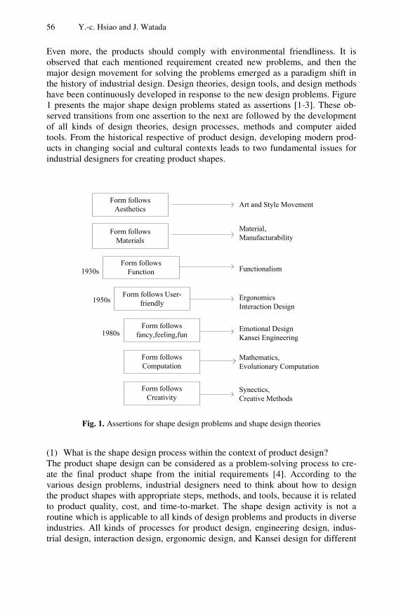
56 Y.-c. Hsiao and J. Watada
Even more, the products should comply with environmental friendliness. It is observed that each mentioned requirement created new problems, and then the major design movement for solving the problems emerged as a paradigm shift in the history of industrial design. Design theories, design tools, and design methods have been continuously developed in response to the new design problems. Figure 1 presents the major shape design problems stated as assertions [1-3]. These ob-served transitions from one assertion to the next are followed by the development of all kinds of design theories, design processes, methods and computer aided tools. From the historical respective of product design, developing modern prod-ucts in changing social and cultural contexts leads to two fundamental issues for industrial designers for creating product shapes.
Form follows Aesthetics
Form follows Materials
Form follows Function
Form follows User-friendly
Form follows fancy,feeling,fun
Form follows Computation
Form follows Creativity
Art and Style Movement
Material,Manufacturability
Functionalism
ErgonomicsInteraction Design
Emotional DesignKansei Engineering
Mathematics,Evolutionary Computation
Synectics,Creative Methods
1930s
1980s
1950s
Fig. 1. Assertions for shape design problems and shape design theories
(1) What is the shape design process within the context of product design? The product shape design can be considered as a problem-solving process to cre-ate the final product shape from the initial requirements [4]. According to the various design problems, industrial designers need to think about how to design the product shapes with appropriate steps, methods, and tools, because it is related to product quality, cost, and time-to-market. The shape design activity is not a routine which is applicable to all kinds of design problems and products in diverse industries. All kinds of processes for product design, engineering design, indus-trial design, interaction design, ergonomic design, and Kansei design for different

Shape Design of Products Based on a Decision Support System 57
design situations have been proposed [5-13]. In practice, many companies such as 3M, IDEO, Microsoft, Philips, Toyota and Xerox also develop their own proc-esses which become the benchmark and standards of the other companies due to their successful product innovations. The product design processes of these corpo-rations have been the subject of many case studies and books [14-15]. Applying their product design processes to a practical project becomes challenging due to the difficulty of associating one of the existing generic product design processes to a current specific design task. Project managers rely on experience and intuition to plan the design process. The selection and customization from the well-known product design processes for current shape design problems is a key issue which is not well studied. Furthermore, the shape design is not an isolated activity within a product design process, as shown in Figure 2. Concurrent engineering has been developed for coordinating all kinds of design processes from various disciplines against the conventional overall process interfaces. The complex network inter-faces in concurrent engineering define when the shape design task is active and how industrial designers are engaged in the product design processes. The shape design activity in concurrent engineering context is more complicated and not easily managed. Some studies consider how to integrate the design processes from different disciplines into the product design process [16-19].
Product Design Process
Engineering Design Process
Industrial Design Process
Ergonomics Design Process
Shape Design Process
Interaction Design Process
Kansei Design Process
Fig. 2. The relationship of shape design process within product design processes
To sum up, industrial designers are faced with the difficulty of planning the
whole shape design process within context of the product design process due to the various design tasks in developing modern products, and to the many options for product design process in practice and literature. The decision on the shape design process for the current design task cannot rely on the industrial designers’

58 Y.-c. Hsiao and J. Watada
intuition and experience only. The quality of decision-making on the planned design process is inadequate in a highly competitive market.
(2) How can the shape design knowledge be effectively applied to solve the prob-lems of creating product shapes? Design of product shapes is usually considered as a black box, because the re-quired thinking and knowledge for designing are inside the designer’s brain. There has been great interest in studying how a designer solves a design problem and creates ideas in design theories. The design activities are investigated through interviewing designers, direct record and observation, and case studies. Takeda indicated that the design solution is obtained by different ways of using knowl-edge to meet the required specification [20]. Cushman identified three ways of using human factor knowledge for shape design: trial-and-error, intuition and design principles [16]. In this paper, the approach is explicitly decomposing the shape design problem into many sub-problems which can be more easily solved by the industrial designer. Therefore, the problem of designing a product shape can be decomposed into several sub-problems which are separately considered with the constraints of functions, ergonomics, emotional sensory, and manufac-turability. Then the designer can synthesize a final product shape from the solu-tions of sub-problems. In this approach, each sub-problem can be easily dealt with using appropriate tools and knowledge. It also becomes feasible to utilize artificial intelligence and technologies in computer science to assist designers in solving the sub-problems. This approach implies that the shape design process should be di-vided into several phases. During each phase, the design problem can be solved by some design methods. John Chris Jones presents a chart for selecting design methods during different phase of shape design processes as a design strategy [4]. Look up a row for input information which should be ready before we want to use a particular design method. Then look up the column for the output after we use the design method. The element in the intersection of row and column shows the design methods. The chart is simple and easy to use, but it cannot show the real interfaces and process for a product design, and the mentioned design methods are not updated. Otto and Wood show a roadmap for selection basic or advanced de-sign methods in a product design process [8]. Unfortunately the detailed roadmap for shape design process is not described.
Figure 3 presents a schema to illustrate the discussed fundamental issues: trans-forming the initial requirements into the final product shape design by planning the right shape design process and using appropriate methods, tools as well as knowledge. This paper presents a framework describing the relationship of prod-uct design problems, product design process, shape design process, shape design methods and tools. Accordingly, designers can use the framework for selecting or creating their own shape design processes, choosing the shape design tools, meth-ods, and using knowledge for their own design problems. The fundamental issues are solved with guidance of the proposed framework in this study.

Shape Design of Products Based on a Decision Support System 59
Initial situation and information fromother product design sub-processes
Planning a Shape Design Process Final product
shapes that meet needs and requirements.
Shape design knowledge,design methods,design tools regarding to function,ergonomices,emotions,and manufacturability
Interface
Interface
Interface
Process 3
Process 2
Process 1
Fig. 3. The schema describing the fundamental issues in product shape design
2 The Framework for Product Design Process
The purpose of the framework is to integrate the design processes across different disciplines as well as the design methods for product shape design under different design tasks in a precise manner. Two features, completeness and flexibility, are considered for designing the framework. The completeness indicates that the framework can be adapted to all kinds of product design tasks. The flexibility allows the framework to be easily expanded with newly developed design proc-esses, methods, and tools. The approach of building the framework is described as follows:
(1) A comprehensive survey is conducted on product design tasks, all kinds of design processes from different disciplines, and their associated methods and tools.
(2) Each design process may be divided into sub-processes to the suitable level of detail. The relationships among the different design processes from the litera-ture are investigated.
(3) The framework of the design processes is built. (4) Finally, the design methods and tools are associated to the design processes in
the framework.
The detail work of the proposed framework is only performed for shape design processes due to the scope of this paper. The framework is discussed from two aspects: the shape design process within the context of product design and its associated shape design methods and knowledge.
When surveying a product design process, engineering design process, and in-dustrial design process, it is found that the terminology is ambiguous in the litera-ture. An engineering design process could nearly represent the product design process in some cases. An industrial design process may be equivalent to the

60 Y.-c. Hsiao and J. Watada
product design process for some industrial designers [21]. It would only refer to a process of creating product form for the others. The product design process may indicate the integration of both engineering and industrial design processes in some publications. Additionally, the detailed link between the engineering design process and industrial design process is not shown in the literature. The distinct terminology about “design processes” in literature results in the difficulty of inte-grating these proposed design processes into a framework. Howard et al. provide a comprehensive survey for engineering design process. They compare all the ter-minology and the proposed process models in literature [22]. Howard et al.’s work assists understanding the complexity of engineering design process. Unfortu-nately, no similar work is done in the industrial design process and product design process. As the terminology is clarified, the relationships of design processes can be classified and compared for further discussion.
Another difficulty in studying the design processes arises from the type of product associated to the corresponding design process. The particular design processes for some products such as mobile phone, copy machines and automo-biles have been developed and disclosed in literature. Development for one type of product can have different design processes under various design tasks. The framework should be able to integrate and represent the design processes under various design tasks for all kinds of products.
2.1 Basic Type of Product Design Process
The first decision situation in planning the product design process is choosing the product category. Products can be classified into one of three categories: technol-ogy-driven product, technology-and-user driven product, or user-driven product. The technology-driven product is focused on the engineering functions while the user-driven product focuses on human-factor functions. The product strategy de-termines the category of the product. The technology-driven approach is usually adopted for developing the product in the infant and growth stages of its life cy-cle – S curve. When the product is mature, the user-driven strategy is used [7]. The product design processes are associated to the product categories. Therefore, the term usage and referred literature for “design processes” to build the frame-work are suggested as follows:
The design process for a technology-driven product is referred to as engineering design process in the literature.
The design process for a user-driven product is referred to as indus-trial design process in the literature.
The design process for a technology-and-user driven product is re-ferred to as industrial design, engineering design, and product de-sign in the literature.
The product design process includes engineering design process and industrial design process in a broad sense.

Shape Design of Products Based on a Decision Support System 61
Each product category is associated to three common types of product design processes as shown in Figure 4. For technology-driven products, the engineering design process is followed by industrial design process. The engineering process is parallel with industrial design process for technology-and-user driven products. The industrial design process leads the engineering design process for user-driven products [7]. An engineering design process dealing with the design of engineer-ing functions in a broad range includes mechanical engineering, electronic engi-neering, and software engineering. The industrial design process is related to the human factors, interaction and aesthetics. The following sections will describe the design processes for each product category in detail.
Fig. 4. Product design process for different categories of products
2.2 Design Process for Technology-Driven Product
The design process for technology-driven products consists of two sub-processes: (1) engineering design process and (2) industrial design process. First, the feasibil-ity of the engineering concept is validated. Next, the product form is created by the industrial design process. To avoid the ambiguity from the same terms being used in the engineering design process and industrial design process, concept design and detail design in the engineering design process are named as engineer-ing concept design and engineering detail design; concept and detail design in the industrial design process are named as industrial concept design and industrial detail design respectively. Configuration design in engineering design process is referred as organization design in the industrial design process.
The detail of engineering design and industrial design processes depends on the type of design task: original design or redesign. The engineering and industrial design processes are quite different for each type of product design task. The de-termination of design tasks as an original design or redesign depends on the corporate strategy for disruptive innovation or continuous innovation. Original

62 Y.-c. Hsiao and J. Watada
design refers to the use of new physical principles to realize the engineering func-tions, significant change of system architecture, or finding new applications for existing platform technologies. The original engineering design process consists of four phases: engineering concept design, configuration design, parameter design, and engineering detail design. Redesign is related to improving the engineering function with the change of component level or the dimension of the products, or modifying the product shape. Redesign can be further classified into three types – part configuration design, variant design, and selection design which only has fewer phases as shown in Figure 5. Part configuration design involves creating the new product architecture. Variant design is related to customizing the existing product by adjusting product parameters. Selection design is about different ways of using standard parts to create a new product. For each phase of engineering design, previous studies can be referred to for details [6-11].
The industrial design process can be decomposed into four phases of the shape design process: organization, surfacing, detail (industrial detail design), and graph-ics from Wallace’s model [23-24]. The organization phase in Wallace’s model is the same as the configuration design which has been performed in engineering design process under original design task. Surfacing phase is to generate enclo-sures in different styles, Details phase is to add details such as local surface altera-tions or new elements to complete the exterior surface, and Graphics phase is to apply graphical elements such as color, screening, decals, hot stampings, and texture to the outer surface of the product. Only three phases follow the engineer-ing detail design as shown in Figure 5. The design principles from ergonomics and Kansei engineering can be applied to each phase.
2.3 Design Process for User-Driven Product
The development of a user-driven product can be referred as a market-pull strat-egy. The development concepts always start from user scenarios, not from techno-logical ideas. The product with complicated technology can belong to the category of user-driven product if the product ideas come from user-scenarios first. The design process for the user-driven product is usually led by industrial designers. The decision of product category is followed by two design situations: original design and redesign as shown in Figure 6. Figure 7 shows the detailed processes for original design and redesign respectively. The industrial designers develop the product concepts by industrial conceptual design process in original design case. Then the designer can consider the spatial arrangement of components from the viewpoints of ergonomics and Kansei in the phase of organization design. At the same time, the project team should consider the feasibility of engineering solu-tions from current proposed ideas. If there is a need to innovate a new engineering solution, engineering concept design and configuration design should be followed. Otherwise, the industrial designer can proceed to surfacing phase. The engineer-ing parameter design related to the dimension of product can be performed before the surfacing phase, or engineers can perform it with consideration of surfacing design from industrial designers. The design principles from ergonomics and Kan-sei design can be applied to surfacing phase. After the surfacing phase, industrial detail design can be performed. When the industrial detail design is finished, the

Shape Design of Products Based on a Decision Support System 63
project team can decide if engineering detail design should be performed before or after the graphics design. During the graphics design phase, the designer can con-sider using the approaches from Kansei design and ergonomics. The difference of the design process between original design and redesign for the user driven prod-uct is that only industrial concept design is included in the design activity of origi-nal design process.
Decision 2
Original Design
E.Configuration Design
F.Parameter Design
G.Engineering Detail Design
D.Engineering Concept Design
Redesign
H.Ergonomics I.Kansei DeignL. Surfacing
M. Industrial Detail Design
M. Graphics
H.Ergonomics I.Kansei Deign
H.Ergonomics I.Kansei Deign
C. Industrial Design Process
B. Engineering Design Process
Decision 3
E.Configuration Design
F.Parameter Design
G.Engineering Detail Design
F.Parameter Design
G.Engineering Detail Design
G.Engineering Detail Design
Selection Design
Variant Design
Part Configuration Design
Fig. 5. Original design and redesign processes for technology-driven products

64 Y.-c. Hsiao and J. Watada
Fig. 6. Design situations for a user-driven product
G.Engineering Detail Design
K.Organization
L.Surfacing
M.Industrial Detail Design
N.Graphics
Decision 5
No
YES
No
Decision 7
No
No
Decision 8
E.Configuration Design
D.Engineering Concept Design
Decision 6
F.Parameter Design
YES
F.Parameter Design
YES
G.Engineering Detail Design
YES
J.Industrial Concept Design
A
BH.Ergonomics
I.Kansei Deign
H.Ergonomics
I.Kansei Deign
H.Ergonomics
I.Kansei Deign
H.Ergonomics
I.Kansei Deign
Fig. 7. Original design and redesign processes for a user-driven product

Shape Design of Products Based on a Decision Support System 65
2.4 Design Process for Technology-and-User Driven Product
The design process for technology-and-user driven products is not specifically discussed in the literature. Many complex technology products demand high-touch user interactions for lowering the learning curve and reducing frustration with the operations of technology products. Thus the design process for this product cate-gory can be analogically described by an interaction design process. Interaction design has evolved with the combination of industrial design and software user interface design since the late 1980s. Interaction design deals with hard-ware/software integration, software application design, and interactive media and content [25]. IDEO proposes a five-stage process for interaction design: under-stand, observe, visualize and predict, evaluate and refine, and implement [26]. IDEO’s design process is used in the framework as shown in Figure 8. During “understand” and “observe” phases, the client is interviewed and the real users’ behaviors are observed. The key problem can be found. Next stage is “visualize and predict” about the concept generation for the key problems. Interdisciplinary team members brainstorm to create concepts. All the requirements from engineering, ergonomic, Kansei, etc are considered at the same time by a group of people. Then detailed design and implementation follow. This design process is quite successful for developing many excellent products in IDEO. The most famous supermarket shopping cart was designed and videoed with this process. General Electric adopts a similar process called CENCOR for designing its products [27]. CENCOR stands for collaborate, explore, create, organize, and realize. Philips has similar design processes for realizing the philosophy of “Sense and Simplicity” [46]. The distinct stages are project planning, briefing, creating, designing, presenting, and drawing. Following IDEO’s processes, this design process for a technology-and-user driven product is shown in Figure 8. It is the same for original design or redesign tasks.
Fig. 8. The design process for a technology-and-user driven product

66 Y.-c. Hsiao and J. Watada
3 Methods and Tools for Shape Design
After the framework of the product design processes is fully built, each sub-process can be effectively associated with the design methods which are proposed in many studies. Figure 10 shows the schema of using design methods and tools. For example, product matrix, structure grammar and morphological method can be used for the configuration design. Style design process can use the tools of shape grammars, and Kansei engineering methods (emotional based engineering method) [26-30]. According to the structure of the framework, new design meth-ods and tools can be easily added to the proposed framework. For example, when developing next-generation creative products, the designers usually sketch the product shapes from void. Then the engineers try to bring the sketches to life. They usually need and find the inspiration from fashion, architecture, and so on to create new shapes for new products. Instead of wandering around the imaginary world, creative thinking methods such as synectics, morphological method, bionic method and analogical thinking have become popular for the designers to open their imagination. Nicolas’s book describes how to create a new shape from crea-tive methods and gives many examples [32]. On the other hand, Bentley’s book asserts that evolutionary computation for arts initiates the interest of researches in the 1990s. One of the examples is the design of the car shapes with various con-figurations and sizes [33]. Now we can add these new tools into the framework as shown in Figure 9.
Fig. 9. The schema for associating a design process with design methods and tools

Shape Design of Products Based on a Decision Support System 67
4 DSS for Planning of Design Process
There are two fundamental issues concerning how to effectively use design knowledge for solving the design problems. The proposed framework resolves the issues conceptually, but it may not provide a friendly way for practical use due to lack of support of storing and reasoning design knowledge. DSS has been widely applied to engineering design, industrial design and product design. To implement the framework, a DSS is considered for the following reasons:
(1) A DSS can facilitate the interaction between an industrial designer and computers to generate alternative plans for design processes.
(2) A DSS can provide unstructured design knowledge stored as rules or any kind of knowledge representation methods for making decision.
(3) A DSS can implement the framework more easily due to the available commercial software programming tools and research efforts in this area.
During the survey of DSS on product design, several types of applications have been found. Besharati et al. use a generalized purchase modeling approach to develop an expected utility metric on customer basis that forms the basis for a DSS to support the selection in product design [34]. Toben and Leo built DSS for selection of manufacturing processes in product design [35]. Giachetti aggregates the decision on material selection and manufacturing process selection into a DSS [36]. Masubana and Nagamachi proposed a hybrid Kansei engineering system to support customers and designers in deciding the kansei of the products [37]. Jindo et al. use semantic difference to find the relationship between customers’ kansei evaluation of office chairs and design elements. The office chair can be created by their proposed DSS [38]. According to the present authors’ best knowledge, no relevant research on DSS for planning of product design process is found. It is assumed that the reason is that the latent need for a better method of planning design process is not revealed and people are satisfied with current approaches to planning the design process. Actually current planning approach is inadequate.
Now we are faced with a new problem: synthesis of a new type of DSS. Our approach is to find an existing type of DSS which is closest to meeting our requirements. Then a new concept of DSS is generated by improving the existing type of DSS until all the requirements are satisfied. According to Power’s taxonomy of DSS, Power differentiates communication-driven DSS, data-driven DSS, document-driven DSS, knowledge-driven DSS, and model-driven DSS by using the mode of assistance as the criterion [39]. Due to the need of the complex and unstructured information in planning a design process, a knowledge-driven DSS is selected as a candidate system for improvement. On the other hand, from the past experience of the researchers, object-oriented programming (OOP) provides many advantages over other tools like C or Prolog in implementing DSS

68 Y.-c. Hsiao and J. Watada
for the conceptual design of products. OOP can facilitate a great visual interface or easy maintenance of DSS. Another key consideration is that object oriented design thinking has been introduced into industrial and product design. Gorti created CONGEN, a decision support system for conceptual design. The CONGEN object is used as a template for constructing an artifact, a design process, and many other objects for recording the design activity from symbolic evolution [40, 41]. The computer support of conceptual design becomes feasible in generating new concepts rather than only for drawing. Bijan et al. used universal modeling language (UML) in OOP to describe the users’ need, scenario of usage, product structure and related design knowledge in product design. The object oriented design leads to a new direction for computer support of product design [42]. OOP provides the advantages of modularization, flexibility and scalability. Integrating an object-oriented and knowledge driven approaches, an object-oriented knowledge-driven DSS is proposed in this paper. It provides a good architecture to support the decision of planning design based on complex design knowledge. The unique feature in the proposed DSS is the symbolic-description of the evolution of the planned design processes. More detail about DSS can be found in Turban and Aronson’s book [43].
The concepts of object-oriented knowledge-driven DSS for planning a design process is validate by a prototype. An object-oriented knowledge-driven DSS has three parts: an object-based decision model, an object-based representation of design process, and an object-based database of design methods. The decision model of planning a design process is described as a decision tree as shown in Figures 4 to 10. Each node in the decision tree is treated as an object of decision class. The attributes of a decision-class object consist of object identifiers, decision description, decision options and decision goals. A process-class object represents the product design processes and sub-processes which are manipulated by the objects of decision class. An object in class of design tool represents an available tool or method associated with many process-class objects. Figure 10 shows the interfaces and interactions with decision makers. The decision history records the transition and status of each decision node in the decision tree. The decision history allows the decision makers to store, retrieve, and modify the results of current planning activities in software. The decision option shows the options of decision for current decision node. The progress of the planned design process and relative information will be shown in the right part of the windows. For example, if the goal of the decision is finding the closest type of product in one of three product categories and technology-driven product is chosen, the software will next decision nodes and current planned design process as shown in Figures 11 and 12. If the buttons of the design processes are pushed, the associate methods and tools will be shown. Due to the huge information related to each design method and tool, the information should be managed by a database. Figure 13 shows the interface of design methods associated to the design process.

Shape Design of Products Based on a Decision Support System 69
Fig. 10. The interfaces of DSS for planning a design process
Fig. 11. The planned design process for a technology-driven product

70 Y.-c. Hsiao and J. Watada
Fig. 12. The planned design process for original design of a technology-driven product
Fig. 13. The interface of design methods associated to a design process.
5 Case Study
The case study of a scooter will illustrate how to use the framework to plan the shape design process and how to create a scooter shape following the planned processes [31].

Shape Design of Products Based on a Decision Support System 71
5.1 Planning of Design Process
The mission statement indicates that a certain corporate needs to develop a new type of scooter for new corporate image. The form style should break the routine image. According to the product strategy in the mission statement, the scooter is positioned as a user-driven product. Industrial design should lead the engineering design. The design task is to redesign the scooter. The design process is shown in Figure 8. The engineering concept is limited to the conventional scooter architec-ture with one front wheel and one rear wheel. The body frame of the scooter has been determined for this case. The major design activities are surfacing and indus-trial detail design where ergonomic design is also considered. For creating a new form style, shape grammar as a design method is used to assist industrial designers creating the concepts of surfacing and industrial detail design. Shape grammars originated from architecture as an expression tool for the form analysis of build-ings and as an inference mechanism for the generative design with a similar archi-tectural style. In recent years, shape grammars have been extensionally applied to the analysis and design of product forms ranging from coffee makers to automo-bile inner hoods. The next section will describe how to create the scooter shapes with shape grammars in planned design process.
5.2 Shape Design in Planned Design Process
Shape grammar is used to create the scooter shape within the design process. Shape grammar is briefly introduced before we go to detailed discussion. Accord-ing to Stiny, G. [44-45], the shape grammar G = (S, L, R, I) consists of four components:
(1) S is a finite set of shapes, (2) L is a finite set of labels, (3) R is a finite set of shape rules of the form α→β where α is a labeled shape in
(S, R)+ , and β is labeled shape in (S, R)*. (4) I is a label shape in (S, R)+ called the initial shape.
S is the set of primitives such as point, line, plane, or solid, circle, or rectangle which are used to construct the shape of the object. The label in L orients the op-eration of rule like the base line or the grid on the background to assist the shape construction. The rule in R is the transformation of the label shape α to the labeled shape β. The arrow → means a shape transformation. For example,
α - a rectangle with a dot label - rotating 45 degrees around its center and shrink-ing the length of edge becomes a labeled diamond-shape - β. The dot label orients the shape of rectangle and diamond. Without the dot label, the rectangular and diamond shapes are equivalent with respect to the rotation. (S, R)+ and (S, R)* represent the sets of left-side and right-side label shapes respectively.

72 Y.-c. Hsiao and J. Watada
Figure 14 illustrates the simple shape grammar to create the designed shape by consecutively applying Rule 1 twice and Rule 2 once. Rule 2 is a terminal rule to remove the dot label.
Fig. 14. A simple shape grammar
After introducing shape grammar, we will discuss the shape grammar associated to the shape design process on creating the scooter shape. Surfacing and industrial detail design processes are focuses.
(1) Surfacing During this phase, the covers of the scooter need to be redesigned with considera-tion of human factors and engineering requirements. The surfaces of the covers need to be designed with a new style for the scooter. The covers are attached to the body frame of the scooter for protecting the internal mechanical part from dust and damage. The body frame of the scooter, wheel sizes, and wheel distance are fundamental engineering considerations. They are known information in this redesign case. They are complied into the shape grammar rules as shown in Rules 1-7 of Figure 15. The human factors such as the posture of the scooter riders are collected. They are represented in a shape grammar as shown in Rules 8 – 11 of Figure 16. Shape grammar specifies the spatial relationship of each cover from Rules 12 – 30 of Figures 17 - 19. The rules can be applied in different ways to generate the new shapes. If the sequence of applying the rules is Rules 1-9, 11, 13, 15, 19, 21, 24, 25, 26, 28, 29, 30, 31, 32, 35, a scooter shape is created as shown in Figure 20. Figure 21 shows the created surface shapes if Rules 1-9, 11, 13, 15, 19, 21, 24, 25, 26, 28, 29, and 30 are applied. The detailed description of rules is listed in Table 2 in Appendix. Shape grammar guides the designer to consider the ergo-nomic and engineering requirements. The real shape of the surface is not explicitly specified in shape grammar in this case study. The emotional factors are consid-ered when applying each rule. The designer can create the surface shape of each cover by the imagination.

Shape Design of Products Based on a Decision Support System 73
Fig. 15. Engineering requirements in Rules 1-7 of shape grammar

74 Y.-c. Hsiao and J. Watada
Fig. 16. Ergonomic requirements in Rules 8-11 of shape grammar
Fig. 17. Surfacing design in Rules 12-15 of shape grammar

Shape Design of Products Based on a Decision Support System 75
Fig. 18. Surfacing design in Rules 16-26 of shape grammar

76 Y.-c. Hsiao and J. Watada
Fig. 19. Rules 27-30 of shape grammar for surfacing design
Fig. 20. Scooter surface created by surfacing design with shape grammar Rules 1-9, 11, 13, 15, 19, 21, 24, 25, 26, 28, 29, and 30
Fig. 21. Scooter surface created by surfacing design with shape grammar Rules 1-9, 11, 13, 14, 18, 22, 24, 25, 26, 28, 29, and 30

Shape Design of Products Based on a Decision Support System 77
(2) Industrial Detail Design During this phase, the detail components of the scooter such as headlight and taillight are attached to the cover surfaces. The spatial relationship of detail com-ponents and covered should be arranged with consideration of engineering requirements. For example, the position of head light can affect the range and distance of illumination of the head light. The types of detail components such as LED or incandescent lamp can also affect the form style. The design rules with consideration of engineering factors can be expressed by the shape grammar as shown in Rules of Figure 21. Assuming that one of the created surfacing shapes after surfacing design, for example, the shape in Figure 19 is selected for further detail design of headlight, front signal light and tail light, two sets of rules can be applied for creating different detail designs as shown in Figures 22 and 23. Figure 23 shows that the headlight is in a lower position near the front fender, the front signal is separate from the headlight, and the taillight is on the rear position of the rear body cover. Figure 24 shows that the set of headlight and front signal light is located on the center part of front cover, and the taillight is attached to the back of the seat. Except different spatial arrangement of detail components, all the shapes of components in two cases of detail design are also created differently.
Fig. 22. Industrial detail design in Rules 31-37 of shape grammar

78 Y.-c. Hsiao and J. Watada
Fig. 23. Scooter detail components created for detail design with shape grammar Rules 1-9,11,13,15,19,21,24,25,26,28,29,30, 31, 32, and 36
Fig. 24. Scooter detail components created for detail design with shape grammar Rules 1-9,11,13,15,19,21,24,25,26,28,29,30,31,33, and 37
6 Conclusion
Development of modern products is a challenging task subject to many con-straints. Two fundamental issues for industrial designers are: what is the shape design process within the context of product design, and how the shape design knowledge can be effectively applied to solve the problems of creating product shapes. After a comprehensive survey of the literature, this paper proposes a framework integrating the product design problems, product design process, shape design process, shape design methods and tools with consideration of the require-ment of function, ergonomic, emotional and manufacturing factors. Accordingly, designers can use the framework on planning their own shape design processes, choosing the shape design tools, methods, for their own design problems. The fundamental issues are resolved with guidance of the proposed framework. The proposed framework is implemented using an object-oriented DSS that can com-pletely integrate all the up-to-date design research into a knowledge base and

Shape Design of Products Based on a Decision Support System 79
provide an interactive interface. Therefore DSS can assist industrial designers to make a better decision on planning of design process and using design methods. A scooter case study illustrates planning the shape design process by using DSS. According to the planned design process, the shape design of a scooter is created by using the shape grammar which integrates the ergonomic and engineering re-quirements. The future efforts will be toward two directions: (1) using case-base reasoning to suggest the design processes based on the similar cases in DSS, (2) allowing industrial designers customizing the design process from the suggestion of DSS. Future DSS will behave more intelligently.
References
1. Bürdek, B.E.: Design History, Theory and Practice of Product Design. Birkhauser, Germany (2005)
2. Bhaskaran, L.: Designs of the Times: Using Key Styles for Contemporary Design. Quayside Pub. Group, New York (2005)
3. Cross, N.: Forty years of design research. Design Studies 28, 1–4 (2007) 4. Jones, J.C.: Design Methods, 2nd edn. Wiley, New York (1992) 5. Suh, N.P.: The Principles of Design. Oxford University Press, USA (1990) 6. Pahl, G., Beitz, W., Wallace, K., Pomeranst, A.: Engineering Design-A Systematic
Approach. Springer, Heidelberg (1999) 7. Ulrich, K.T., Eppinger, S.D.: Product Design and Development. McGraw Hill, New
York (1997) 8. Otto, K.N., Wood, K.L.: Product Design: Techniques in Reverse Engineering and New
Product Development. Prentice Hall, New York (2001) 9. Ullman, D.G.: The Mechanical Design Process, 3rd edn. McGraw Hill, New York
(2004) 10. Clausing, D., Fey, V.: Effective Innovation: The Development of Winning Technolo-
gies. ASME Press, New York (2004) 11. Eggert, R.J.: Engineering Design. Prentice Hall, New York (2005) 12. Hsiao, S.-W., Chou, J.-R.: A creativity-based design process for innovative product
design. International Journal of Industrial Ergonomics; Vol 34, 421–443 (2004) 13. Terninko, J.: Step-by-Step QFD: Customer-driven product design. CRC Press, Boca
Raton (1997) 14. Myerson, J.: IDEO Masters of Innovation. Te Neues Publishing Company, New York
(2005) 15. Morgan, J.M., Liker, J.K.: The Toyota Product Development System: Integrating Peo-
ple. In: Process and Technology, Productivity Press, USA (2006) 16. Cushman, W.H.: Human Factors in Product Design. Elsevier Science Publishers, New
York (1991) 17. Broberg, O.: Integrating ergonomics into the product development process. Interna-
tional Journal of Industrial Ergonomics 19, 317–327 (1997) 18. Oakes, G.L., Felton, A.J., Garner, K.B.: From the formal to the innovative: The use of
case studies and sustainable projects in developing a design process model for educat-ing product/industrial designers. European Journal of Engineering Education 31, 567–579 (2006)

80 Y.-c. Hsiao and J. Watada
19. Tung, F.-W., Deng, Y.-S.: A Study on Integrating Interaction Design into Industrial Design Processes. In: The 6th Asia Design International Conference, Tsukuba, Japan (2003)
20. Takeda, H.: Toward Multi-aspect Design Support Systems. Technical Report NAIST-IS-TR94006, Nara Institute of Science and Technology, Nara, Japan (1994)
21. Kressy, M.: Industrial Design, Lecture Notes in MIT Open Course Ware Lec-ture:15.783J Product Design and Development (2006)
22. Howard, T.J., Culley, S.J., Dekoninck, E.: Describing the creative design process by the integration of engineering design and cognitive psychology literature. Design Stud-ies 29, 160–180 (2008)
23. Wallace, D.R.: A computer model of aesthetic industrial design. M.S. Thesis, Massa-chusetts Institute of Technology (1991)
24. Wallace, D.R., Jakiela Mark, J.: Automated Product Concept Design: Unifying Aes-thetics and Engineering. IEEE Computer Graphics & Applications 134, 66–75 (1993)
25. Morggridge, B.: Designing Interactions. MIT Press, Cambridge (2007) 26. Spreenberg, P., Salomon, G., Joe, P.: Interaction Design at IDEO Product Develop-
ment 27. Okude, N.: デザイン思考の道具箱: イノベーションを生む会社のつくり方
Hayakawa Publishing, Japan (2007) 28. Hsiao, S.-W., Chen, C.-H.: Semantic and shape grammar based approach for product
design. Design Studies 18, 275–296 (1997) 29. Manish, A., Cagan, J.: A blend of different tastes: the language of coffee maker. Envi-
ronment and Planning B: Planning and Design 25, 205–226 (1998) 30. Pugliese, M.J., Cagan, J.: Capturing a rebel: modeling the Harley-Davidson brand
through a motorcycle shape grammar. Research in Engineering Design 4, 139–156 (2002)
31. Hsiao, Y.C., Watada, J.: Systematic construction of shape grammars for form design of products. Kansei Engineering International 8 (2009)
32. Roukes, N.: Design Synectics: Simulating Creativity in Design. Elsevier Science & Technology Books, New York (1988)
33. Bentley, P.J., Corne, D.W.: Creative Evolutionary Systems. Baker & Taylor Books (2001)
34. Bessarati, et al.: A decision support system for product design selection: a generalized purchase modeling approach. Decision Support Systems 42, 333–350 (2006)
35. Lenau, T., Alting, L.: Intelligent Support Systems for Product Design. Annals of the ClRP 38 (1989)
36. Giachetti, R.E.: A decision support system for material and manufacturing process se-lection. Journal of Intelligent Manufacturing 9, 265–276 (1998)
37. Matsubara, Y., Nagamachi, M.: Hybrid Kansei Engineering System and design sup-port. International Journal of Industrial Ergonomics 19, 81–92 (1997)
38. Jindo, T., Hirasago, K., Nagamachi, M.: Development of a design support system for office chairs using 3-D graphics. International Journal of Industrial Ergonomics 15, 49–62 (1995)
39. Power, D.J.: Decision support systems: concepts and resources for managers. Quorum Books, Westport, Conn (2002)
40. Gorti, R.: From Symbol to Form: A framework for design revolution. Ph.D. disserta-tion, MIT (1995)
41. Gorti, S.R.M., et al.: An object-oriented representation for product and design proc-esses. Computer-aided design 30, 489–501 (1998)

Shape Design of Products Based on a Decision Support System 81
42. Aryana, B., et al.: Application of Object Oriented Thinking in Product Design: Design Process of Personal Digital Partner. In: International Association of Societies of De-sign Research, pp. 12–15. Hong-Kong Polytechnic University (2007)
43. Turban, E., Aronson, J.E.: Decision Support Systems and Intelligent Systems. Pren-tice-Hall, Englewood Cliffs (2001)
44. Stiny, G.: Introduction to shape and shape grammars. Environment and Planning B: Planning and Design 7, 343–351 (1980)
45. Stiny, G.: Shape: Talking about seeing and doing. MIT Press, Cambridge (2006) 46. Marzano, S.: Past Tense, Future Sense: Competing with Creativity: 80 Years of
Design at Philips. BIS Publishers, Netherlands (2005)

82 Y.-c. Hsiao and J. Watada
Appendix: Terminology of Design Processes and Shape Grammar Rules
Table 1. Terminology of Design Processes
A. Product Design Process Product Design Process includes tasks of creating, tasks of understand-ing, and tasks of communication, task of testing, and task of persuasion. Any product development process includes three phases: understand the opportunity, develop a concept, and implement a concept [8].
B. Engineering Design Process Engineering Design is the set of decision-making process and activities used to determine the form of an object given the functions desired by the customer [11].
C. Industrial Design Process Industrial design process is the set of activities to create the shape style design. It can be divided into two parts: ergonomic design and shape style design. Ergonomic design considers the factors such as cost and safety of the product, and the interaction of user-interface. Style design deals with the division of competitive products in market, the product image of owner [7].
D. Engineering Concept Design Engineering Concept Design is the part of the engineering design process in which, by the identification of the essential problems through abstrac-tion, by the establishment of function structures and by the search for appropriate working principles and their combination, the basic solution path is laid down through the elaboration of a solution principle [6].
E. Configuration Design A phase of design when geometric features are arranged and connected on a part, or standard components or selected for the architecture [11].
F. Parameter Design A phase of design that determines specific values for the design variables [11].
G. Engineering Detail Design A phase of design that results in the preparation of a package of informa-tion that includes drawings and specifications sufficient to manufacture a product [11].
H. Ergonomics/Human Factors To describe the abilities, limitations, and other physiological or behav-ioural characteristics of humans that affect the design and operation of tools, machines, systems, task jobs, and environments. Ergonomics is a synonym frequently used by practitioners in Europe [11].
I. Kansei Design A translating technology of the consumer's psychological feeling (Kan-sei) and image about a coming product into design elements [47].

Shape Design of Products Based on a Decision Support System 83
J. Industrial Concept Design Industrial Concept Design generates the aesthetic of the product and the interaction of human–machine interface in the industrial design process [7].
K. Organization Organization performs spatial positioning of components in form creat-ing process [24].
L. Surfacing Surfacing generates an enclosure for the product design [24].
M. Industrial Detail Design Industrial detail level deals with local surface alterations or new elements to complete the exterior surface [24].
N. Graphics Graphics level applies the elements such as colouring, surface textures, decals and hot stampings to the outer surface of the product [24].
O. Understand Understand helps establish a common language between the customer’s needs and design team and initiates development of a design team that bridges both organizations [26].
P. Observe Observe the information of key users doing key tasks. The people and tasks observed are carefully selected to cover the space of the design problem [26].
Q. Visualize & Predict To synthesizing the information and envision key interaction ideas. As interaction ideas emerge – and the exact process whereby they do emerge is rather unpredictable and undocumentable – they are visualized in simulations suitable for informal evaluation [26].
R. Evaluate & Refine Setting the test strategy to evaluate the result of visualization, and the re-finement of the design based on feedback. Designs typically pass through several iterations of visualization and evaluation before a design is finalized. The end result is often a synthesis of the designers’ intui-tions and feedback from users’ evaluations [26].
S. Implement Product form design, a detailed design, a full specification of interaction methods and their representations are implemented [26].

84 Y.-c. Hsiao and J. Watada
Table 2. Description of Shape Grammar Rules
Engineering requirements Rule 1: The initial shape is a point with a label O at the origin of the coordinate system. Define the original point as the axle center of the rear wheel. Rule 2: the axial position of the front wheel is defined by the wheelbase length. Rule 3: the bottom boundary line is created for ground clearance. Rule 4: the length and rake angle of the front fork is specified. Rule 5: the profile of the body frame is added. Rule 6: the swing arm is connected to the body frame. Rule 7: the wheels are added. Ergonomic requirements Rule 8: the footrest line is created. Rule 9: the foot of seated human is on the footrest line. Rules 10 – 11: Either Rules 10 or 11 are applied to add the straight or Y-shape handle bar. The position of the hands and the front fork constrains the selection of rules. Surfacing design Rules 12 - 13: If the Rule 10 is selected, Rule 12 should be followed to add the instrument console; otherwise, Rule 13 should be applied. Rules 14 – 16: One of the rules should be applied to attach the front cover. Rule 17: There is no front cover Rules 18 - 20: The inner cover should cover the front fork partially and match with the shape of the front cover. One of the rules is selectively applied to add the inner cover. Rule 21-22: Two types of front fenders can be selected Rule 23: There is no front fender. The front cover works as the function of the front fender. Rule 24: the side cover is attached to the front cover side by side. Rule 25: the center cover is located above the side cover. Rule 26: the body cover is connected to the side cover and the center cover. Rule 27: there are no side cover, center cover, and body cover. Rule 28: the seat is added. Rule 29: the rear fender is created. Rule 30: the footrest panel is created. Industrial detail design Rule 31: the headlight is on the front cover. Rule 32: the front turning signal is on the front cover, but it is not integrated with the headlight. Rule 33: the integral set of headlight and front turning signal is on the front cover. Rule 34: the taillight is created. Rule 35: the rear turning signal is created. Rule 36: the integral set of taillight and rear turning signal is attached on the body cover. Rule 37: the integral set of taillight and rear turning signal is attached on the seat.

L.C. Jain and C.P. Lim (Eds.): Handbook on Decision Making, ISRL 4, pp. 85–116. springerlink.com © Springer-Verlag Berlin Heidelberg 2010
Chapter 4
Enhancing Decision Support System with Neural Fuzzy Model and Simple Model
Visualizations
Eng Yeow Cheu1, See Kiong Ng2, and Chai Quek1
1 Centre for Computational Intelligence, Nanyang Technological University, Singapore
[email protected], [email protected] 2 Institute for Infocomm Research,
A*STAR (Agency for Science, Technology and Research) [email protected]
Abstract. Decision making and knowledge creation processes are interde-pendent as the process of decision making itself will result in improved un-derstanding of the problem and the process, and generates new knowledge. The integration of decision support and knowledge management can en-hance the quality of support to decision makers, and providing quality support is key to decision support system (DSS). However, people have cognitive constraints to fully understand the support they get from DSS. This paper presents a new approach to solving model externalization by tak-ing into consideration the imprecise nature of decision makers' judgements on the different tacit models. Knowledge in the form of highly intuitive and easily comprehensible fuzzy rules is created using a neuro-fuzzy system called the Tree-based Neural Fuzzy Inference System (TNFIS). TNFIS em-ploys a novel structure learning algorithm that is inspired from the Piaget's constructivist emphasis of action-based cognitive development in human. Simple visualization techniques of the explicit neuro-fuzzy model are also proposed in this paper to enhance the internalization ability of the knowl-edge workers. Results from the experiments show that TNFIS is able to rep-resent the formulated explicit model using a set of concise and intuitive fuzzy rules knowledge base, and achieve better or comparable generaliza-tion than other models. Visualizations of the formulated TNFIS model are also shown to enhance the decision maker's understanding of the problem domain and subsequent internalization of the selected model.
1 Introduction
The overwhelming flow of data, information, and knowledge from an increasing number of sources will continue to grow and become even more complex. This has underlined the need for some form of decision support system (DSS) to handle the

86 E.Y. Cheu, S.K. Ng, and C. Quek
ever increasing complexity in the context for effective planning, problem solving, decision making, and the carrying out of business operations and management [1, 2].
The concept of DSS was defined by Gorry and Scott Morton [3], who com-bined Anthony's categories of management activity [4], and Simon's intelligence, design, and choice description of the decision-making process [5]. In their frame-work, intelligence comprises of the search for conditions calling for decision, design involves the development of possible solutions to the problem, and choice consists of analyzing and selecting one of the solutions for implementation. Figure 1 illustrates the model of the decision-making process in a DSS environment. The decision process in Fig. 1 emphasizes the problem analysis and the model devel-opment. Once the problem is recognized and defined, alternative solutions are created and the models are subsequently developed to analyze the various alterna-tives. A choice is subsequently made and implemented. This framework is consis-tent with Simon's description [5]. Generally, these stages overlap and loop back to earlier stages as more information is obtained about the problem.
Fig. 1. The DSS decision-making process modified from [6]
DSS has evolved from two main areas of research: the theoretical studies of or-ganizational decision making and the technical work [7]. With advancement in computer technology, new computerized DSS were developed and studied. Today it is still possible to reconstruct the history of DSS. Two broad categories of DSS have been defined and they are: model-based, and knowledge-based decision sup-port systems [6, 8].
Model-based DSS can be divided into three stages: formulation, solution, and analysis. Formulation stage involves the generation of a model in a form accept-able to a knowledge worker. The solution stage refers to the development of the model to solve the problem. The analysis stage refers to the analyses and interpre-tation of the model solution. In the analysis stage, the model solution is delivered

Enhancing DSS with Neural Fuzzy Model and Simple Model Visualizations 87
in a usable form to enhance the ability to analyze and understand the problem and the solution. This approach is consistent with Simon's intelligence, design, and choice description of the decision-making process [5].
Knowledge-based DSS is a system that can capture, organize, leverage, and disseminate not only data and information but also knowledge about the firm. Knowledge-based DSS can improve the mental model(s) and understanding of the decision makers(s) by providing interesting patterns and up-to-date decision mod-els that can be retrieved and shared across the organization.
The need for active decision support was asserted by Keen, and Carlsson et al. [9, 10]. The functions of a DSS is “to extend their (decision makers) capabilities but not to replace their judgement” and “to support the solution of a certain problem” as defined by Turban et al. [11]. DSS is also classified by Arnott and Pervan [12] as “the area of information systems discipline focussed on supporting and improving mana-gerial decision making”. It is the support that is the key importance of DSS. The key problems of using DSS is not totally technology-related but more of people-related problems [10, 13, 14]. People have cognitive constraints to genuinely fully compre-hend the support they obtain from DSS. Often the problems and decisions are too ill-defined to be sufficiently codified and embedded within a computer program. Human decision making capability can be supported and enhanced by the use of a DSS to make better decisions and more effectively deal with unstructured or semi-structured, difficult problems without extensive experience and expert knowledge.
Most organizations view knowledge as a strategic resource, and to make use of that knowledge on decision making a strategic capability [15]. Two very different knowledge management strategies are in place: personalization strategy or codifica-tion strategy [16]. In personalization strategy, knowledge is shared mainly through person-to-person contacts and the main purpose of computers is to help people communicate. For codification strategy, knowledge is carefully codified and stored in databases, where it can be accessed and used by anyone in the organization.
In the process of decision-making, decision makers combine different type of data and knowledge available in various forms in the organization. Decision making and knowledge creation processes are interdependent as the process of decision making itself will generally result in an improved understanding of the problem and the proc-ess, and generates new knowledge. Decision support and knowledge management can be integrated to enhance the quality of support provided to decision makers [17]. Figure 2 illustrates a framework proposed by Bolloju et al. for developing enterprise decision support environments combined with knowledge management. This frame-work integrates the Nonaka's model of knowledge creation process [18], in which organizational knowledge is created through a continuous dialogue between four patterns of interaction involving tacit and explicit knowledge. These four patterns of interaction are: socialization, externalization, combination, and internalization.
Modern organizations now are able to collect and maintain huge volumes of data in data warehouses. A data warehouse provides the knowledge workers with basic factual information. However, only a fraction of the overwhelming amount of data may be required. In addition, identifying the relevant information may be difficult if not impossible. Unless the knowledge workers understand the informa-tion about the data they are working on, a data warehouse does not necessarily provide the knowledge workers adequate support.
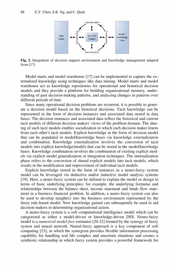
88 E.Y. Cheu, S.K. Ng, and C. Quek
Soci
aliz
atio
n Combination
Fig. 2. Integration of decision support environment and knowledge management adapted from [17]
Model marts and model warehouse [17] can be implemented to capture the ex-ternalized knowledge using techniques like data mining. Model marts and model warehouse act as knowledge repositories for operational and historical decision models and they provide a platform for building organizational memory, under-standing of past decision-making patterns, and analyzing changes in patterns over different periods of time.
Since many operational decision problems are recurrent, it is possible to gener-ate a decision model based on the historical decisions. Tacit knowledge can be represented in the form of decision instances and associated data stored in data bases. The decision instances and associated data reflect the historical and current tacit models of different decision makers' views of the problem domain. The shar-ing of such tacit models enables socialization in which each decision maker learns from each other's tacit models. Explicit knowledge in the form of decision model that can be populated in model/knowledge bases via knowledge externalization and combination. Knowledge externalization involves the conversion of tacit models into explicit knowledge/models that can be stored in the model/knowledge bases. Knowledge combination involves the combination of existing explicit mod-els via explicit model generalization or integration techniques. The internalization phase refers to the conversion of shared explicit models into tacit models, which results in the modification and improvement of individual tacit models.
Explicit knowledge stored in the form of instances in a neuro-fuzzy system model can be leveraged via deductive and/or inductive model analysis systems [19]. Here, a neuro-fuzzy system can be utilized to explain the model or design in terms of basic underlying principles; for example, the underlying formulae and relationships between the balance sheet, income statement and funds flow state-ment in a business financial problem. In addition, a neuro-fuzzy system can also be used to develop insight(s) into the business environment represented by the fuzzy rule-based model. New knowledge gained can subsequently be used to aid decision makers in determining organizational action.
A neuro-fuzzy system is a soft computational intelligence model which can be categorized as either a model-driven or knowledge-driven DSS. Neuro-fuzzy model is a numerical model-free estimator [20-22] formed by the synergy of fuzzy system and neural network. Neural-fuzzy approach is a key component of soft computing [23], in which the synergism provides flexible information processing capability for handling real life complex and uncertain situations and creates a symbiotic relationship in which fuzzy system provides a powerful framework for

Enhancing DSS with Neural Fuzzy Model and Simple Model Visualizations 89
expert knowledge representation while neural network supplements the fuzzy system with the learning capabilities suitable for computationally efficient hard-ware implementation [24-28].
Neural network itself lacks the explanation capability which is a requirement for the accountability of the decisions in many business problems. Simplicity of the explicit model representation in terms of fuzzy rules is particularly suitable for the decision makers to understand and internalize. Neuro-fuzzy model thus is able to describe a problem domain using a linguistic model. The linguistic model pro-vides an explicit declarative representation of knowledge about the problem domain, in the form of a set of highly intuitive and easily comprehensible fuzzy if-then rules. This explanatory capability of the neuro-fuzzy model can also be used in the verification of the internal logic of the model where the internal states of the system can be accessible and unambiguously interpreted. This explanatory mechanism allows the platform for a novice decision maker to gain insights into the problem at hand. Decision makers may also use the fuzzy rules to identify regions in the input space which are not sufficiently represented in the model, and to accordingly supplement the explicit model with tacit models. In addition, where there exist human experts whose knowledge can be incorporated in the form of if-then rules to existing explicit models via knowledge combination [29]. In this context, refinement to the decision model may be performed. Neuro-fuzzy model-ling is suitable for incremental learning in which new knowledge in the form of fuzzy rules can easily be integrated into and inappropriate knowledge can be eliminated from the existing DSS model/knowledge bases. Knowledge bases pro-vide the decision maker with an intelligent analytical platform for socialization, articulation, integration, and understanding of knowledge management. The use of a natural language-generated knowledge provides the ability to validate the mod-els, and identify new knowledge created in the process.
In addition, uncertainty inherently exists in almost all modern real world com-plex problems. The incorporation of fuzzy set theory within neuro-fuzzy system creates a soft computing decision model that is able to take advantage of the knowledge in natural-language form that provides the ability to deal with impreci-sion and uncertainty.
This paper presents a new approach to solving model externalization by taking into consideration the imprecise nature of decision makers' judgements on the dif-ferent tacit models. Decision making processes involving ill-structured or semi-structured problems are more subjectively represented as decision makers tend to employ their intuition and experience in the process. The different views are ex-pressed using different fuzzy sets. Knowledge in the form of fuzzy rules is created using a neuro-fuzzy system called the Tree-based Neural Fuzzy Inference System (TNFIS). TNFIS employs a novel structure learning algorithm that is inspired from the Piaget's constructivist emphasis of action-based cognitive development; motor actions rather than sensory inputs dictate the form of the network [30]. Simple visualization techniques of the explicit neuro-fuzzy model are also proposed in this paper to enhance the internalization ability of the knowledge workers.
This paper is organized as follows. Section 2 provides a brief review of some ex-isting neuro-fuzzy systems and particularly those systems that incorporate decision tree. Section 3 briefly describes TNFIS that has been proposed in [31]. Section 4

90 E.Y. Cheu, S.K. Ng, and C. Quek
gives examples using TNFIS in the model externalization of tacit models, namely, Nakanishi [32], gas furnace [33], and iris flowers [34] data sets. Visualizations of the explicit TNFIS models are also provided to assist the knowledge worker to internalize the explicit knowledge discovered. Section 5 concludes this paper.
2 Related Works
One of the first papers incorporating neural network and fuzzy logic as keywords was published in 1974 [35]. Lee et al. proposed a fuzzy neuron that was general-ized from the M-P neuron model [36]. To date, there are many different ap-proaches to building an integrated neural-fuzzy system in addition to the different views in categorization of these hybrid systems [22, 37-39]. Regardless of how these systems are categorized, the fundamental rationale for the integration of both systems is that to incorporate the strengths from the respective systems. In the following sections, some existing neuro-fuzzy systems [38], as well as, the incor-poration of decision tree that attempts to synergize both approaches; namely: fuzzy systems and neural-fuzzy integrated systems are discussed.
2.1 Neuro-fuzzy Systems
The major drawback of fuzzy logic systems is their inability to adapt and learn. Neural network, on the other hand, is employed to augment the fuzzy rule based system with a learning method that is able to systematically tune the parameters of the fuzzy rule based system, such as the parameterized fuzzy sets representing the linguistic terms of the fuzzy rule based system. Such an integrated system is termed as the neuro-fuzzy system [38].
Some existing neuro-fuzzy systems treat the use of neural network as a compo-sition of functions (membership functions, aggregation operators, fuzzy connec-tives, defuzzification methods). Analytical procedures are then applied to tune the parameters of one of those functions based on the evaluation of an objective func-tion. Systems employing this concept are [39-52], in which membership functions are tuned using the gradient descent method.
Systems from [50, 53-55] perform an unsupervised classification (clustering) during the initial stage so as to derive the initial partitions of the input space. Membership functions are subsequently constructed from these partitions. This type of systems is very much constrained by the clustering method being per-formed in the initial stage, and more importantly, will further be aggravated by any clustering method based on spatial density due to the sparsity of data in high dimensional space [56]. Furthermore, a good cluster may represent different classes of data patterns and different clusters may contain data patterns from one class [57]. In addition, as noted by Duda and et al. [58], it is more important to discriminate when the aim is to distinguish data patterns; namely:
“While it is a truism that ideal representation is the one that makes classification easy, it is not always so clear that clustering without explicitly incorporating clas-
sification criteria will find such a representation.” ([58] (p.581))
Enhancing DSS with Neural Fuzzy Model and Simple Model Visualizations 91
Hence, a fuzzy rule created from a cluster may not represent the correct correla-tion between the particular localized input and associated output space. The other drawback with using clustering method is the need for user to specify the number of clusters which consequently define the number of rules.
Other systems [39, 46, 48, 59] employ some form of clustering algorithm (competitive learning) to firstly tune the linguistic membership functions. Rules are then selected by some criteria during the competitive learning phase. Super-vised learning to train the parameters of the linguistic membership functions is performed during the last phase.
The neuro-fuzzy systems as proposed in [39, 46, 48, 51] generally employ five layers partially connected feedforward neural network structure to describe the Mamdani type fuzzy rules in the system. The second and fourth layer of the net-work represents the input and output fuzzy labels respectively. The resultant parti-tion of the data spaces is essentially the fuzzy grid [60]. Fuzzy grid partitioning is the most restrictive as the fuzzy rules share the available input and output linguis-tic terms. For classification task, fuzzy logic systems using fuzzy grid partitioning and without the use of certainty factors to describe the rules basically become loop-up table classifiers when the number of rules is increased [61, 62]. This approach contradicts the whole idea of introducing fuzzy set theory to handle uncertainty.
While some form of certainty factors are introduced in the other systems [48, 51], these parameters are only used for consistent rule generation during the struc-ture learning phase. Fuzzy rules being encoded in their networks are essentially rules without certainty factors. The neuro-fuzzy systems from [39, 46, 48, 49, 51, 52] in which all possible rules are first populated and are subsequently pruned. This list-all-then-prune approach generally requires large amount of memory space as the initial stage require the storage of all rule information. These systems suffer from the exponential increase in the amount of rules when dimension of data increases. Some works that aim to reduce the amount of rules are LazyPOP learning algorithm [63], and RSPOP [64].
2.2 Integration of Decision Tree
The objective of neuro-fuzzy models is to construct a fuzzy logic system that is able to forecast and explicate the behavior of the unknown system. The modelling task is usually performed in two stages: structure identification and parameter learning. Structure learning is related to determining a suitable number of rules, feature selection scheme, and a proper partitioning of the feature space. Issues remain to be addressed are identifying a good structure for fuzzy inference system in the face of the "curse of dimensionality", as well as, the optimum number of rules. Jang [65] suggested that the integration of decision tree and neuro-fuzzy system can alleviate these issues.
Decision trees are non-parametric method capable of handling data sets with missing values and extremely well suited in high-dimensional data analysis. Deci-sion tree can extract distinct rules and select relevant inputs to create a roughly correct and compact structure with high degree of interpretability. Such models closely resemble human reasoning. They are based on the divide and conquer

92 E.Y. Cheu, S.K. Ng, and C. Quek
methodology in partitioning the feature space into mutually exclusive region. They tend to perform well if few highly relevant attributes exist. Decision trees are unstable classifiers as they are very sensitive to perturbation of training data. Noise and irrelevant attributes can highly affect their performance.
Soft decision tree [66] is a variant of classical decision tree inductive learning with the incorporation of fuzzy set theory. Fuzzy technique is integrated in soft decision tree during the growing process of the tree. Classical decision tree tech-nique has been shown to be interpretable, efficient, problem-independent and able to handle large scale applications. A major drawback of classical decision tree is that they are highly unstable classifiers with respect to minor perturbations in the training data. The incorporation of fuzziness into classical decision tree improves the stability of decision tree.
Other approach that derives a neural network from classical decision tree can be found in [57, 60, 67-73]. Both AFLN [69], and F-CID3 [71] inherit their net-work structure from a decision tree. The fundamental principle is to map the struc-ture of the decision tree onto a feedforward neural network. The decision neuron of the network is associated with a function that is used to represent a membership function. AFLN network is subsequently tuned with quickprop algorithm [74], while F-CID3 is tuned with Cauchy training method [75] which is a form of gradi-ent descent method. F-CID3 is an extension to CID3 algorithm [68] which incor-porates fuzzy set theory.
Lin et al. [57] initialized a four layers feedforward neural network with the rules generated from a heuristically binary tree-like partition algorithm. The input feature space is recursively partitioned at fix locations until either difference in the output labels between the two generated bins is considered insignificant or mini-mum number of data points is reached.
MoDFuNC [73] which is inspired from SuPFuNIS [50] has its structure ini-tially identified by CART decision tree. High certainty and low certainty rules generated by the CART decision tree are then mapped onto a neuro-fuzzy system. Rules of low certainty generated by CART can be further divided into a subset of secondary rules that use an extended set of variables. This is to allow a fine identi-fication of the patterns in these partitions associated with the low certainty rules.
The initial organization of the neural network is realized by the utilization of decision tree in which input patterns that respond to same action (belonging to the same class) are grouped together and input patterns that respond to different actions are segregated. The employment of decision trees in the structure identifi-cation phase resembles Piaget's cognitive view of action-driven cognitive devel-opment process manifested in human.
3 TNFIS: A Computational Model Inspired from Piaget's Action-Based Cognitive Development
In this section, the structure and learning algorithm of TNFIS [31] are briefly presented.
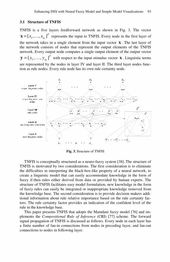
Enhancing DSS with Neural Fuzzy Model and Simple Model Visualizations 93
3.1 Structure of TNFIS
TNFIS is a five layers feedforward network as shown in Fig. 3. The vector T
nxx ],,[11 …=x represents the input to TNFIS. Every node in the first layer of
the network takes in a single element from the input vector x . The last layer of the network consists of nodes that represent the output elements of the TNFIS network. Every output node computes a single output element of the output vector
Tnyy ],,[
51 …=y with respect to the input stimulus vector x . Linguistic terms
are represented by the nodes in layer IV and layer II. The third layer nodes func-tion as rule nodes. Every rule node has its own rule certainty node.
Fig. 3. Structure of TNFIS
TNFIS is conceptually structured as a neuro-fuzzy system [38]. The structure of TNFIS is motivated by two considerations. The first consideration is to eliminate the difficulties in interpreting the black-box-like property of a neural network, to create a linguistic model that can easily accommodate knowledge in the form of fuzzy if-then rules either derived from data or provided by human experts. The structure of TNFIS facilitates easy model formulation, new knowledge in the form of fuzzy rules can easily be integrated or inappropriate knowledge removed from the knowledge base. The second consideration is to provide decision makers addi-tional information about rule relative importance based on the rule certainty fac-tors. The rule certainty factor provides an indication of the confident level of the rule in the knowledge base.
This paper presents TNFIS that adopts the Mamdani fuzzy model [76] and im-plements the Compositional Rule of Inference (CRI) [77] scheme. The forward signal propagation of TNFIS is discussed as follows. Every node in each layer has a finite number of fan-in connections from nodes in preceding layer, and fan-out connections to nodes in following layer.

94 E.Y. Cheu, S.K. Ng, and C. Quek
Layer I: Input Linguistic Nodes There are n1 nodes in this layer. A node in layer I represents an input linguistic variable. The node only propagates the non-fuzzy input value to the linguistic term
nodes of the corresponding linguistic variables in the layer II. The net input Iif
and net output Iio of the ith linguistic are described in (1),
., Ii
Iii
Ii foxf ==
(1)
Layer II: Input Linguistic Term Nodes
There are ∑=
=1
12
n
iiJn linguistic term nodes in the second layer. Each linguistic
term node represents a membership function of a particular input fuzzy variable. The input linguistic term node jiA , denotes the jth input linguistic label of the ith
linguistic variable. jiA , is derived from a bell-shape membership function. The net
input IIjif , and net output II
jio , of the input linguistic term node jiA , are given
in (2),
.,)(2
)(,
,2,
2,
,
IIjifII
jiIIji
IIji
IiII
ji eoco
f =−
−=σ
(2)
In (2), IIjic , and II
ji ,σ are respectively the center and width of the Gaussian mem-
bership function of the jth linguistic label of the ith input linguistic variable. The operation of the linguistic term nodes is equivalent to the singleton fuzzification of the input.
Layer III: Rule Nodes A node in this layer represents a fuzzy rule. Every rule node performs the fuzzy AND operation. The net input III
kf and net output IIIko of the kth rule node are
defined in (3),
.,.),(
,III
kIIIk
Aji
IIji
IIIk
IIIk foowf
IIIk
== ∏∈
(3)
In (3), IIIkA is the set of the antecedent nodes (input linguistic term nodes) in layer
II that are connected to the kth rule node in layer III, and IIIkw represents the rule
certainty factor of the kth rule. Every rule certainty node is attached to a rule node in layer III, and each rule
node in layer III has only one rule certainty node attached to it. The rule certainty factor is derived from the output of a sigmoidal function described by (4),

Enhancing DSS with Neural Fuzzy Model and Simple Model Visualizations 95
.1
1IIIk
IIIk u
IIIk
ew
λ−+= (4)
In (4), IIIkλ determines the steepness of the sigmoidal function of the kth rule cer-
tainty node.
Layer IV: Output Linguistic Term Nodes
There are ∑=
=5
14
n
mmLn nodes in this layer. Every node in this layer represents an
output linguistic term/label and performs the fuzzy OR operation on all fuzzy rules leading to the same consequent. The net input IV
lmf , and net output IVlmo , of the
output linguistic term node lmC , are defined in (5),
.),(max ,,,,
IVlm
IVlm
IIIk
Rk
IVlm foof
IVlm
==∈
(5)
In (5), IVlmR , is the set of rule nodes in layer III that are connected to the lth conse-
quent node in layer IV of the mth output linguistic variable.
Layer V: Output Linguistic Nodes A node in this layer represents the output linguistic variable. The following func-tion as defined in (6) is used to simulate the center of area defuzzification method. The net input V
mf and net output Vmo of the mth output linguistic variable are de-
fined in (6),
.,
,,1,,,,1
,,, ∑∑=
=
==
m
m
Ll
IVlm
IVlm
VmV
mLl
IVlm
IVlm
IVlm
Vm
o
foocf
…… σ
σ (6)
In (6), mL is the total number of output linguistic term nodes in layer IV associated
with the mth output variable, and IVlmc , and IV
lm,σ are respectively the center and
width of the lth linguistic term of the mth output linguistic variable.
3.2 Learning Algorithm of TNFIS
The learning algorithm for the proposed neuro-fuzzy system consists of two phases: Piaget's action-based structure learning phase, and a parameter tuning phase.
Piaget's Action-Based Structure Identification Phase In this section, the Piaget's cognitive view of action-driven cognitive development process in human that is employed in the structure identification of TNFIS is discussed.

96 E.Y. Cheu, S.K. Ng, and C. Quek
The fundamental difference between Piaget and cognitivist psychology lies in their respective views with respect to language. Cognitivist psychology usually views all mental activity as symbolic processing, whereas for Piaget, language is viewed as only one aspect of cognition which is derived from non-linguistic (sen-sory-motor) cognition. Piaget views that intelligence is basically non-linguistic and is derived from action, not from language [30].
The distributed characteristic of a neural network, in which the inputs are mapped to the outputs through an internal organization of the neural network (network's architecture and connection weights), resembles Piaget's definition of a schema. A schema is an adaptive device that automatically assimilates new inputs to already existing schemata and accommodates existing schemata as a function of new inputs. It is necessary that the initial organization of the neural network is realized by the structure learning phase such that the network obeys the following two general principles:
1. To make the input patterns that respond to the same action more similar to each other,
2. To make the input patterns that respond to different actions more different from each other.
These two general principles are achieved by the structure learning algorithm. The aim of the structure learning algorithm is to segregate the decision instances asso-ciating with different degrees to the different actions. The structure learning phase consists of two steps. In the first step, the data instances are first segregated. In the second step, fuzzy rules are generated from the data groupings discovered in the first step. These fuzzy rules are subsequently mapped into the structure of TNFIS. For example, classification of a set of decision instances into a set of distinct classes is a generic type of problem that is commonly employed in real life deci-sion making environments. Credit approval, securities trading, product selection, risk estimation, and customer selection are some examples of classification prob-lems. The first step of the algorithm would group the data instances according to the decision maker's judgement about the different type of classes, and the second step would associate the different groups of data instances to one of the decision maker's classes.
For illustration simplicity, let us consider only one output variable. A data pair
);,,( 1,,1, 1 pnpp yxx … is assigned an output linguistic value lC ,1 as defined in (7) if,
qlLqlyy pCpC ql≠=> ;,,1,);()( 11,1, ,1,1
…μμ . (7)
In (7), 1L is the number of output linguistic terms. The output linguistic label that
a data pattern has the maximum membership grade is assigned to the data pattern as described by (7). At the end of this step, every data pattern is tagged to a par-ticular output linguistic term based on the corresponding output data pattern mem-bership grade to the output linguistic term.
The objective of the first step is to determine the partitioning of the input fea-ture space such that every partition in the input feature space contains as many data patterns tagged with the same output linguistic label. The input feature data

Enhancing DSS with Neural Fuzzy Model and Simple Model Visualizations 97
space is iteratively divided until either the maximum number of splits allowable on every feature axis has been reached or when all partitions contain data patterns belonging to the same output linguistic term. Since a pattern can belong partially to different output linguistic labels, the splitting criterion is based on the soft clas-sification error impurity measure (see (8)) that is derived from the classification error impurity measure [78].
With every split, the whole feature space is partitioned into a finite number of hyper-rectangular cells. Each cell is evaluated for its soft classification error. The soft classification error )(cEsoft
for the cth cell is evaluated as in (8),
.)(max1)( ,1
1
cCFcE lsoft
L
lsoft −= (8)
In (8), )( ,1 cCF lsoft represents the relative soft frequency of the data patterns to an
output linguistic label lC ,1 in the cth cell, and is computed in (9),
.
)(
)(
)(1
,1
,1
1 11,
11,
,1
∑∑
∑
= =
==L
q
N
ppC
N
ppC
lsoftc
q
c
l
y
y
cCF
μ
μ
(9)
In (9), cN represents the number of data patterns contained in partition c. Equa-
tion (9) takes the membership grades of the data patterns with respect to other output linguistic labels into consideration as well. If delta functions are used to represent the output membership functions (for classification task), (9) reduces to the relative accuracy of the data patterns belong to output linguistic label lC ,1 in
the c cell. The split that results in the minimum weighted soft classification error is se-
lected. The minimum weighted soft classification error is computed as in (10),
.)(1
cEN
NE soft
N
c
csoft
space
∑=
= (10)
In (10), spaceN represents the total number of subspaces created by a split, and N
represents the total number of data patterns. After the series of splits, the input feature space is divided into a grid contain-
ing finite number of hyper-rectangular crisp-boundary partitions/cells. These crisp partitions are subsequently converted into fuzzy partitions having fuzzy decision boundaries by employing Gaussian membership function. Each Gaussian mem-bership function is used to represent a split segment of a feature axis. The center of the Gaussian function for the first and last segment of a feature is set to the corresponding minimum operating range value and maximum operating value respectively. For other segments, the center of the Gaussian function is set as the average of corresponding split segment end points. The width of the correspond-ing Gaussian membership function is then computed to satisfy ε-completeness.

98 E.Y. Cheu, S.K. Ng, and C. Quek
This first step illustrates the fact that the initial organization of a sensory-motor neural network is dictated by the motor actions (consequent/class labels) with which an organism must respond to the various sensory inputs. With the given motor actions (output linguistic terms), the data space partition algorithm groups inputs if those inputs must be responded to with the same motor action, and sepa-rates inputs if those inputs must be responded to with different motor actions. This implies that it is action rather than sensory input that dictates the form of the neu-ral network and is in agreement with Piaget's constructivist emphasis of action-based view knowledge in the development of cognition [30].
In the second step, the fuzzy rules are generated based on the fuzzy partitions from the first step. For every non-empty input fuzzy partitions, a fuzzy rule is created with the antecedent part of the rule corresponds to the input fuzzy sub-space. A non-empty fuzzy partition is a subspace that contains at least a data pattern with at least ε membership grade for every input linguistic variable. The patterns enclosed by the fuzzy partition converted from crisp partition are also those that are originally enclosed by the crisp partition. The consequent part of the
corresponding fuzzy rule kR is assigned with the most dominant output linguistic
term k
lC
,1 as defined in (11),
.,,1);(maxarg
),()).((
1,1
1,,1
,1
,1
1
,,1
LldominantC
yxdominant
l
lk
jil
Cl
kl
ppartitionp
Cip
n
iAC
…==
= ∑ ∏∈ =
μμ (11)
In (11), kjiA ,
μ represents the membership grade of the jth input linguistic label of
the ith input variable associated with the kth rule, lC ,1
μ represents the membership
grade of the lth output linguistic label of the first output variable.
The fuzzy rule kR is assigned rule certainty factor IIIkw defined as in (12),
IIIkw .,,1;
)max(1
1
1
,1
,1 Ll
dominant
dominantL
lC
C
l
l …==
∑=
(12)
Parameter Tuning Phase In this phase, the parameters of the TNFIS networks are fine tuned by a supervised gradient-descent learning scheme based on the error back-propagation algorithm [79]. The instantaneous error between the output of the network and the desired value is feedback into the network to adjust the parameters of the fuzzy member-ships and rule certainty factors.

Enhancing DSS with Neural Fuzzy Model and Simple Model Visualizations 99
4 Numerical Experiments
In this section, TNFIS is evaluated on four different experiments. The time-series forecasting performance of TNFIS is evaluated on a nonlinear system and a hu-man operation of a chemical plant from the Nakanishi data set [32], and Box-Jenkins gas furnace data set [33]. The last experiment is performed to evaluate the classification performance of TNFIS on Iris flowers [34].
4.1 Nakanishi Data Set
In this section, experiments to evaluate the performance of the proposed system are carried out on two data sets that have been reported by established work [32, 64, 80]. These two data sets are: a nonlinear system, and the human operation of a chemical plant. Each of the data sets1 [32] consists of three groups of data pat-terns: A, B, and C. The data patterns in group A and B are employed as training samples and the other data patterns in group C are employed as the test samples. This set up is similar to the validation method as reported in [32]. The result for this experiment is consolidated in Table 3.
Nakanishi Data Set 1: A Nonlinear System The nonlinear system is described by (13),
( )25.12
211 −− ++= xxY . (13)
In this experiment, our aim is to evaluate the effectiveness of our structure learn-ing algorithm in the identification of the initial structure for TNFIS. The process to be modelled is described by the mapping in (14),
( ) yxx →21, . (14)
The initial output linguistic terms are assumed to be equally spaced within the output operating range using three Gaussian membership functions. This is shown in Fig. 4(e). Given these initial output fuzzy sets, every data point is labelled with a particular output fuzzy set using the procedure discussed in Sect. 3. The result-ing feature space is partitioned into nine subspaces as shown in Fig. 5. The data points belonging to different class labels (output linguistic terms) are plotted with different markers. The dash lines represent the split values that are selected. The data space partitioning algorithm attempts to segregate the different classes of data points into separate partitions.
The fuzzy membership functions that describe the input variables x1 and x2 are shown in Fig. 4(a) and Fig. 4(c) respectively. Six fuzzy rules are generated and these fuzzy rules are shown in Table 1. These rules are used to initialize the
1 Please take note that the Y value of the fifth data point in Group A of nonlinear system
data set provided by [27] is incorrect. Y should be equal to 3.11 instead of 1.97. The
nonlinear system is modelled by ( )25.12
211 −− ++= xxY .

100 E.Y. Cheu, S.K. Ng, and C. Quek
structure of TNFIS. The parameter learning phase is subsequently performed to fine tune the parameters of the fuzzy membership functions and rule certainty factors. The adapted membership functions are shown in figures 4(b), 4(d), and 4(f). The rule certainty factors are adapted as shown in Table 1.
Table 1. Rule base generated from nonlinear system training data samples
Rule IF THEN Certainty factor
x1 x2 y Before adapted After adapted %Δ
1 MF1 MF2 MF3 0.94116 0.94985 0.923329 2 MF2 MF1 MF3 0.69387 0.80058 15.3786 3 MF2 MF2 MF2 0.83246 0.26509 -68.1558 4 MF2 MF3 MF2 0.55072 0.090266 -83.6095 5 MF3 MF2 MF2 0.78585 0.88877 13.09665 6 MF3 MF3 MF1 0.87616 0.88092 0.54328
%Δ = percentage change of rule certainty factor
Nakanishi Data Set 2: Human Operation of a Chemical Plant In this experiment, an operator's control of a chemical plant is examined. The chemical plant produces a polymer by the polymerization of some monomers. An operator determines the set point for the monomer flow rate and the actual value of the monomer flow rate for the plant is controlled by a PID controller. There are five input variables which a human operator might refer to for his control of the output monomer flow rate. Only three input variables are used in this example. The process is described by (15),
( ) yxxx →321 ,, . (15)
In (15), x1 represents the monomer concentration to the plant, x2 represents the change of monomer concentration, x3 represents the monomer flow rate, and y the set point for monomer flow rate.
The initial and adapted membership functions for the input and output variables are illustrated in Fig. 6. Table 2 depicts the fuzzy rules that are generated to de-scribe the model.
Table 2. Rule base generated from human operation of chemical plant data set
Rule IF THEN Certainty factor
x1 x2 x3 y Before adapted After adapted %Δ
1 MF1 MF1 MF2 MF2 0.68802 0.72678 5.63357 2 MF1 MF2 MF3 MF3 0.77484 0.80284 3.613649 3 MF1 MF3 MF3 MF3 0.89837 0.88406 -1.59288 4 MF2 MF1 MF2 MF2 0.82639 0.8263 -0.01089 5 MF2 MF3 MF2 MF2 0.65155 0.65616 0.707544 6 MF2 MF3 MF3 MF3 0.85172 0.85386 0.251256 7 MF3 MF1 MF1 MF1 0.59417 0.59404 -0.02188 8 MF3 MF2 MF1 MF1 0.88095 0.87514 -0.65952 9 MF3 MF2 MF2 MF2 0.88565 0.888667 0.11517 10 MF3 MF3 MF1 MF1 0.88989 0.89594 0.679859 11 MF3 MF3 MF2 MF2 0.88738 0.88215 -0.58938
%Δ = percentage change of rule certainty factor

Enhancing DSS with Neural Fuzzy Model and Simple Model Visualizations 101
0 1 2 3 4 5 60
0.2
0.4
0.6
0.8
1
MF1 ↓
MF2 ↓
MF3 ↓
MFs for input variable x1
(a) initial: x1
0 1 2 3 4 5 60
0.2
0.4
0.6
0.8
1
MF1 ↓
MF2 ↓
MF3 ↓
MFs for input variable x1
(b) final: x1
0 1 2 3 4 5 60
0.2
0.4
0.6
0.8
1
MF1 ↓
MF2 ↓
MF3 ↓
MFs for input variable x2
(c) initial: x2
0 1 2 3 4 5 60
0.2
0.4
0.6
0.8
1
MF1 ↓
MF2 ↓
MF3 ↓
MFs for input variable x2
(d) final: x2
0 1 2 3 4 5 60
0.2
0.4
0.6
0.8
1
MF1 ↓
MF2 ↓
MF3 ↓
MFs for variable y
(e) initial: y
0 1 2 3 4 5 60
0.2
0.4
0.6
0.8
1
MF1 ↓
MF2 ↓
MF3 ↓
MFs for variable y
(f) final: y
Fig. 4. Initial and adapted membership functions of the nonlinear system data set
1 1.5 2 2.5 3 3.5 4 4.5 51
1.5
2
2.5
3
3.5
4
4.5
5
↑2
↑1x
1
x 2
3 →
4 →
Fig. 5. Feature space partitioning of the nonlinear system data set

102 E.Y. Cheu, S.K. Ng, and C. Quek
3.305 4.47 5.635 6.8 7.9650
0.2
0.4
0.6
0.8
1
MF1 ↓
MF2 ↓
MF3 ↓
MFs for variable x1
(a) initial: x1
3.305 4.47 5.635 6.8 7.9650
0.2
0.4
0.6
0.8
1
MF1 ↓
MF2 ↓
MF3 ↓
MFs for variable x1
(b) final: x1
-2.635 -1.7 -0.765 0.17 1.1050
0.2
0.4
0.6
0.8
1
MF1 ↓
MF2 ↓
MF3 ↓
MFs for variable x2
(c) initial: x2
-2.635 -1.7 -0.765 0.17 1.1050
0.2
0.4
0.6
0.8
1
MF1 ↓
MF2 ↓
MF3 ↓
MFs for variable x2
(d) final: x2
-2914.5 401 3716.5 7032 10347.50
0.2
0.4
0.6
0.8
1
MF1 ↓
MF2 ↓
MF3 ↓
MFs for variable x3
(e) initial: x3
-2914.5 401 3716.5 7032 10347.50
0.2
0.4
0.6
0.8
1
MF1 ↓
MF2 ↓
MF3 ↓
MFs for variable x3
(f) final: x3
-2750 500 3750 7000 102500
0.2
0.4
0.6
0.8
1
MF1 ↓
MF2 ↓
MF3 ↓
MFs for variable y
(g) initial: y
-2750 500 3750 7000 102500
0.2
0.4
0.6
0.8
1
MF1 ↓
MF2 ↓
MF3 ↓
MFs for variable y
(h) final: y
Fig. 6. Initial and adapted membership functions of the human operation of a chemical plant data set

Enhancing DSS with Neural Fuzzy Model and Simple Model Visualizations 103
Discussion In this experiment, both the data sets can be viewed as the tacit models which are represented by sets of related attribute values pertaining to various outcomes for the time-series forecasting problem. The model externalization process converts such tacit models into explicit models in the form of fuzzy rule knowledge base using TNFIS that can be easily represented and stored in a typical relational data-base management system. Visualizations of the explicit model such as the mem-bership functions plot can be used together with the knowledge base to enhance the understanding of the underlying problem domain.
In the first example, visualizations of the explicit model such as Fig. 4 and Fig. 5, and the knowledge base that is shown in Table 1 can be leveraged to en-hance the knowledge workers' understanding of the explicit knowledge. By using this information, a knowledge worker can deduce that a small value (near 1) for the input variables x1 or x2 of the nonlinear system will generally produce a high value (of over 4) for the output variable y. In addition, the rule certainty factors shown in Table 1 indicate the relative importance of the rules in the knowledge base. For example, rule 4 has a very low certainty factor. In this case, a knowledge worker may totally ignore that knowledge in his decision or consider input values described by rule 4 having an output value more likely described by the output membership function MF1 since this example is a time-series forecasting problem. Alternatively, knowledge worker may use the visualizations and knowledge base to identify regions in the input space which are not sufficiently represented in the existing model, and to supplement the data instances accordingly.
In the second example, a decision maker may find a high correlation between input variable x3 and the output variable y. Both the variables are described by three membership functions, and the knowledge base discovered using the model formulated by TNFIS as shown in Table 2 indicates that. In this example, the human may simply rely on the monomer flow rate x3 to control the plant to achieve the desired monomer flow rate y. This example illustrates that the knowl-edge base and the visualization plot of the membership functions can be utilized to simplify the operation of such system and validate the operation of the human operator. Hence, the knowledge base for this example can be minimized to just three rules using three membership functions to describe the input variable x3 and output variable y. The linguistic model incorporated in the neuro-fuzzy model provides the capability to internalize the explicit model otherwise not easily com-prehensible as a weight vectors within a neural network.
Instead of analyzing the possibly huge amount of tacit models (decision in-stances) from the data bases, these two examples illustrate that the explicit models can be shared among other decision makers that allow other decision makers to easily internalize the new relationships discovered between the key factors.
In addition to the benefits of TNFIS being a neuro-fuzzy system to providing comprehensible knowledge base for solution explanation, TNFIS is able to formu-late the model with high degrees of generalization accuracy. Table 3 shows the generalization performance of some neuro-fuzzy models in terms of Mean Squared Error (MSE) results on the unseen data instances for the above two data sets. TNFIS outperforms all other model formulation methodologies. This can be

104 E.Y. Cheu, S.K. Ng, and C. Quek
seen in Table 3 in which TNFIS is able to achieve about 5.5 fold improvement than the best model (POP-CRI) on data set 1, and about 8 fold improvement than the best model (DENFIS) on data set 2.
Table 3.Experimental Results on Nakanishi Data Sets
Model Set 1 (Nonlinear System)
Set 2 (Chemical Plant)
POP-CRIa 0.270 5.630 × 10⁵ RSPOP-CRIa 0.383 2.124 × 10⁵ Sugeno (P-G)a 0.467 1.931 × 10⁶ Mamdania 0.862 6.580 × 10⁵ Turksen (IVCRI)a 0.706 2.581 × 10⁵ ANFISa 0.286 2.968 × 10⁶ EFuNNa 0.566 7.247 × 10⁵ DENFISa 0.411 5.240 × 10⁴ TNFIS 0.051 6.8506 × 10³ a Adapted from [64]
4.2 Box and Jenkins's Gas Furnace
The ability of TNFIS in system identification is examined by employing the well-known and widely utilized gas furnace data [33]. This data set was derived from a combustion process of methane-air mixture. During the process, the amount of methane was adjusted while keeping the gas flow rate into the gas furnace con-stant. The resulting C02 concentration is then measured from the gases from the outlet of the furnace. The data consists of 296 successive observations sampled at 9s interval. Every observation records the methane gas feed rate in cubic feet per minute and the corresponding percentage of C02 in the outlet gas. The process to be modelled is described by (16),
( ) ( )( ) )(, 21 tytytx →−− ττ (16)
In (16), x(t) represents the measured gas flow rate into the furnace, y(t) is the C02 concentration in the outlet gas, and τ1 and τ2 are set to 4 and 1 respectively.
In this experiment, 292 observations from the original data set with input data containing the methane flow rate at time t-4 and C02 produced at time t-1, and the output data containing the C02 produced at time t. The task of TNFIS is to identify the soft computing model for the current output C02 concentration y(t) given the amount of methane gas four time steps before (x(t-4)) and the previous C02 con-centration (y(t-1)).
Fuzzy rules are generated based on 200 training samples randomly selected from the 292 data pairs. The initial membership functions are shown in figures 7(a), 7(c), 7(e). The rule base generated by the TNFIS structure learning phase is shown in Table 4. The resulting membership functions are shown in figures 7(b), 7(d), and 7(f). The rule certainty factors are adapted as shown in Table 4.

Enhancing DSS with Neural Fuzzy Model and Simple Model Visualizations 105
-0.5 0 0.5 1 1.50
0.2
0.4
0.6
0.8
1
MF1 ↓
MF2 ↓
MF3 ↓
MF4 ↓
MF5 ↓
(a) initial: x(t-4)
-0.5 0 0.5 1 1.50
0.2
0.4
0.6
0.8
1
MF1 ↓
MF2 ↓
MF3 ↓
MF4 ↓
MF5 ↓
(b) final: x(t-4)
-0.5 0 0.5 1 1.50
0.2
0.4
0.6
0.8
1
MF1 ↓
MF2 ↓
MF3 ↓
MF4 ↓
MF5 ↓
(c) initial: y(t-1)
-0.5 0 0.5 1 1.50
0.2
0.4
0.6
0.8
1
MF1 ↓
MF2 ↓
MF3 ↓
MF4 ↓
MF5 ↓
(d) final: y(t-1)
-0.5 0 0.5 1 1.50
0.2
0.4
0.6
0.8
1
MF1 ↓
MF2 ↓
MF3 ↓
MF4 ↓
MF5 ↓
(e) initial: y(t)
-0.5 0 0.5 1 1.50
0.2
0.4
0.6
0.8
1
MF1 ↓
MF2 ↓
MF3 ↓
MF4 ↓
MF5 ↓
(f) final: y(t)
Fig. 7. Initial and adapted membership functions of Box-Jenkins gas furnace model
Figure 8 illustrates the effect of rule certainty factors on the firing strengths and decision regions of the fuzzy rules. Fig. 8(a) and Fig. 8(b) respectively illustrates the effect of rule certainty factors on the firing strengths and decision regions of the fuzzy rules. Figures 8(c) and 8(d) illustrate the effect of the same fuzzy rules with-out the incorporation of rule certainty, that is with equal weightage, on the rule firing strengths and decision regions respectively. The numberings in Fig. 8 repre-sent the indices of the consequent membership functions. Figures 8(b) and 8(d) depict the regions in the input data space that are associated to the different conse-quences (actions). These consequences are represented by different colours. For those input data subspaces that are described by all the possible equal-weight fuzzy rules, the decision boundaries between these rules are always parallel to the feature axes (see Fig. 8(d)). This is in contrast to the same area in the data space as shown in Fig. 8(b) which illustrates that the decision boundaries between these same fuzzy rules that have different certainty factors. The use of rule certainty factors moder-ates the rigidness in the fuzzy grid-based partitioning of the data space.

106 E.Y. Cheu, S.K. Ng, and C. Quek
Table 4. Rule base generated from 200 randonly selected Box-Jenkins gas furnace data samples
Rule IF THEN Certainty factor
x1 x2 y Before adapted After adapted %Δ
1 MF1 MF5 MF5 0.83685 0.83577 -0.12906 2 MF2 MF3 MF3 0.67772 0.85225 25.75252 3 MF2 MF4 MF4 0.65478 0.58409 -10.796 4 MF2 MF5 MF4 0.77279 0.58762 -23.9612 5 MF3 MF2 MF2 0.68344 0.53656 -21.4913 6 MF3 MF3 MF3 0.73009 0.4482 -38.6103 7 MF3 MF4 MF3 0.79787 0.75567 -5.28908 8 MF3 MF5 MF4 0.69092 0.83774 21.24993 9 MF4 MF1 MF2 0.62053 0.62808 1.216702 10 MF4 MF2 MF2 0.824 0.84503 2.552184 11 MF4 MF3 MF2 0.69985 0.72945 4.229478 12 MF5 MF1 MF1 0.69755 0.69834 0.113254 13 MF5 MF2 MF1 0.58219 0.5753 -1.18346
%Δ = percentage change of rule certainty factor
(a) firing strength
(b) decision region
(c) firing strength (equal certainty factor)
(d) decision region (equal certainty factor)
Fig. 8. Firing strengths and decision regions of rules for the gas furnace model (numbers represent the indices of consequent MF)
In addition, Fig. 8 provides an insight to the operation of the gas furnace. The methane feed rate generally has a negative effect on the future CO2 concentration. The explicit knowledge base stored in the form of fuzzy rules can also be leveraged to deduce this finding. Hence, the operation of this gas furnace can be simplified by considering just the methane gas flow rate to control the CO2 concentration.

Enhancing DSS with Neural Fuzzy Model and Simple Model Visualizations 107
Table 5 lists the comparative results of the different modelling approaches per-formed on the Box-Jenkins gas furnace data. More comparative results can be found in [81, 82]. TNFIS effectively models a nonlinear process with good gener-alization capability comparable to other models. TNFIS has about 3 fold im-provement in terms of MSE better than Pedrycz's model and comparable to ANFIS [83] which is a fuzzy TSK model [84]. The best model (Chebyshev NN) achieves almost 2 fold improvement in terms of MSE better than TNFIS. However Chebyshev NN makes use of 6 input variables and each input variable is expanded to two Chebyshev polynomial terms. In additional, Chebyshev NN does not pro-duce a linguistic model.
Table 5. Performance of different modelling methods on Box-Jenkins gas furnace data
Model Training cases
No. of inputs No. of Rules (parameters)
MSE on normalized data (×10-3)
MSE on unnormal-ized data
Nie’s model[85]
unknown 4 (y(t-1), x(t-3), x(t-4), x(t-5))
45 (225) 0.169
Pedrycy’s model[86]
unknown 18 77 (152) 0.3950a
ANFIS [87] 145 2 (x(t-4), y(t-1)) 4 (24) 0.653b 145 2 (x(t-4), y(t-1)) 25 (105) 0.814b 200 random 2 (x(t-4), y(t-1)) 4 (24) 0.567b 200 random 2 (x(t-4), y(t-1)) 25 (105) 0.525b HyFIS [88] 200 random 2 (x(t-4), y(t-1)) 13 (95) 1.5
200 random + 92
2 (x(t-4), y(t-1)) 15 (105) 0.42
Multi-FNN [89] 296 2 (x(t-3), y(t-1)) 0.028c, 0.265d Chebyshev NN[90]
296 6 - (12) 0.0695
TNFIS 200 random 2 (x(t-4), y(t-1)) 13 (43) 0.575 0.1277 0.494c, 0.753d 0.109c, 0.167d
a MSE is stated as N
k kk dy1
2)(2
1 in [86]
b Best result obtained based on program file bjtrain.m provided in [87] c MSE on training data d MSE on test data
4.3 Iris Classification
In this section, the learning ability and the generalization ability of TNFIS in the classification problem is examined. For this experiment, the Iris data set [34] from the UCI repository of machine learning databases is used. The problem requires the classification of three species of iris flowers, namely, Iris Setosa, Iris Versi-colour, and Iris Virginica.
Learning Ability for Training Patterns The learning ability of TNFIS is examined by evaluating the resubstitution accu-racy of TNFIS on the iris data set. In this experiment, all the 150 patterns of the iris data are employed as the training samples. After the training, the same patterns are used as test patterns to evaluate the resubstitution accuracy of the trained network.

108 E.Y. Cheu, S.K. Ng, and C. Quek
Table 6 shows the resubstitution accuracy of some models evaluated on the iris data. The value of K for TNFIS in Table 6 indicates the maximum number of fuzzy sets for every feature axis, whereas the value of K for other models repre-sents the number of fuzzy sets for every feature axis. Table 6 illustrates that the learning ability of TNFIS is generally better than the other methods for all values of K with the exception when K=3. The result in Table 6 also shows that the num-ber of rules generated by TNFIS is significantly much lesser than all other models.
Table 6. Learning Ability for Iris Training Patterns
Model K = 2 K = 3 K = 4 K = 5 K = 6
Racc (%Δacc)
Nr (%r)
Racc (%Δacc)
Nr (%r)
Racc (%Δacc)
Nr (%r)
Racc (%Δacc)
Nr (%r)
Racc (%Δacc)
Nr (%r)
Adaptivea 94.00 (0)
16 (0)
100.00 (0)
62 (0)
100.00(0)
129 (0)
100.00(0)
190 (0)
100.00 (0)
295 (0)
Simple- fuzzy-grida
67.33 (-28.37)
16 (0)
94.00 (-6)
62 (0)
92.67 (-7.33)
129 (0)
96.00 (-4)
190 (0)
98.67 (-1.33)
295 (0)
TNFIS 96.67 (+2.84)
9 (-43.75)
98.00 (-2)
21 (-66.13)
100.00(0)
45 (-65.12)
100.00(0)
67 (-64.74)
100.00 (0)
76 (-74.24)
Racc: Resubstitution accuracy in terms of percentage %Δacc: Percentage improvement over the maximum resubstitution accuracy obtained by other model Nr: Number of rules %r: Percentage of the maximum number of rules required by other model a Result adapted from [91]
Generalization Ability for Iris Testing Patterns In this experiment, the generalization ability of TNFIS is evaluated by using the same validation methods as performed in [91]. The two methods are, two-fold cross validation (denoted as 2CV), and leave-one-out (denoted as LV1).
For 2CV, the iris data is randomly divided into two subsets, with each subset containing 75 patterns. Each time, one of the subsets is used for training and the other for testing. We iterated 2CV for ten times. Table 7 illustrates that TNFIS possesses superior classification performance than other models. TNFIS is able to constantly classify the iris flowers with a high degree of about 95% classification accuracy. Table 7 also illustrates that there is greater improvement in classification performance for TNFIS at low values of K. For example, TNFIS is able to cor-rectly classify about 3.8% more data patterns than best method at K = 2 and 0.29% more at K = 6. This is mainly due to the fact that impurities are more likely to be included in coarse fuzzy partitions. On the other hand, the input data space is par-titioned by the TNFIS structure learning algorithm to minimize the soft classifica-tion error. This explains the greater classification performance of TNFIS for low values of K. For higher values of K, fuzzy partitions get finer. The likeliness of including different data patterns belonging to other class labels is smaller, thus this explains the similar classification performance achieved by various methods when fuzzy partitions become finer.
Table 8 shows more information about the iris models created by our method. A high mean value of the classification accuracy indicates a high percentage of correct classifications over all the 20 iris models. A small value of the standard

Enhancing DSS with Neural Fuzzy Model and Simple Model Visualizations 109
deviation of the classification accuracy indicates better tolerance to data varia-tions. Table 8 also shows the number of rules required to model the iris data for various values of K.
Table 7. Generalization Ability for Iris Testing Patterns (10 × 2CV)
Model K = 2 K = 3 K = 4 K = 5 K = 6
Cacc (%Δacc)
Cacc (%Δacc)
Cacc (%Δacc)
Cacc (%Δacc)
Cacc (%Δacc)
Adaptivea 91.73 (0)
94.80 (0)
94.53 (0)
94.80 (-0.493)
95.37 (-0.209)
Simple-fuzzy-grida 69.27 (-24.485)
92.43 (-2.5)
90.03 (-4.76)
95.27 (0)
95.57 (0)
TNFIS 95.267 (+3.855)
95.867 (+1.125)
95.867 (+1.414)
95.933 (+0.696)
95.867 (+0.311)
Cacc: Classification accuracy %Δacc: Percentage improvement over the maximum classification accuracy obtained by other model a Result adapted from [91]
Table 8. TNFIS Generalization Ability for Iris Testing Patterns (10 × 2CV)
TNFIS K = 2 K = 3 K = 4 K = 5 K = 6
Minimum accuracy 90.667 92 93.33 95.2 93.33 Maximum accuracy 100.00 98.667 98.667 98.667 98.667 Mean accuracy 95.267 95.867 95.867 95.933 95.867 Standard deviation of accuracy 2.0047 1.977 1.4923 1.588 1.4923 Minimum number of rules 6 16 21 29 37 Maximum number of rules 10 26 39 42 45 Mean number of rules 8.5 20.25 29.5 36.5 41 Standard deviation of the number of rules 1.0513 3.567 4.9364 3.5318 2.5752
For LV1, one iris sample is selected as test pattern, and the other 149 iris samples are used as training patterns to train the network. The procedure is iterated for 150 times, each time by selecting a new sample as test pattern. A total of 150 iris models are created and we calculate the average classification accuracy of these models. Table 9 shows the average classification accuracies of various methods under LV1 validation method. TNFIS is able to achieve higher classification accuracy than other methods for all values of K. Table 10 shows more information about the 150 iris models generated by our method. The standard deviations of classification accu-racy as shown in table 10 are higher that in Table 8 is due to the fact that only one sample is used as test pattern, and that it is either classified correctly or not.
It is also shown in table 10 that the variation of the number of rules generated generally becomes larger when the value of K increases. A larger variation of the number of rules generated can be seen as a larger variation in terms of the model complexity. Although there is higher variation in the model complexity, the incorporation of fuzzy method into the system helps to reduce the variation in classification accuracy. This can be seen in table 10 that consistent performance in classification accuracy is achievable by TNFIS with a generally increasing varia-tion of the number of rules from K = 2 to 6.

110 E.Y. Cheu, S.K. Ng, and C. Quek
Table 9. Generalization Ability for Iris Testing Patterns (LV1)
Model K = 2 K = 3 K = 4 K = 5 K = 6
Cacc
(%Δacc) Cacc
(%Δacc) Cacc
(%Δacc) Cacc
(%Δacc) Cacc
(%Δacc)
Adaptivea 92.00 (0)
95.33 (0)
98.00 (0)
94.67 (-0.692)
96.67 (0)
Simple-fuzzy-grida 67.33 (-26.815)
93.33 (-2.098)
89.33 (-8.847)
95.33 (0)
96.67 (0)
TNFIS 98.667 (+7.247)
98.667 (+3.5)
98.667 (+0.681)
96.667 (+1.402)
97.33 (+0.683)
Cacc: Classification accuracy %Δacc: Percentage improvement over the maximum classification accuracy obtained by other model a Adapted from [91]
Table 10. TNFIS Generalization Ability for Iris Testing Patterns (LV1)
TNFIS K = 2 K = 3 K = 4 K = 5 K = 6
Minimum accuracy 0 0 0 0 0 Maximum accuracy 100 100 100 100 100 Mean accuracy 98.667 98.667 98.667 96.667 97.33 Standard deviation of accuracy 11.508 11.508 11.508 18.011 16.165 Minimum number of rules 9 20 42 55 60 Maximum number of rules 9 30 51 70 77 Mean number of rules 9 21.613 45.147 66.12 74.813 Standard deviation of the number of rules 0 1.69 1.5474 2.593 2.6276
5 Conclusion
In this paper, the effectiveness of a neuro-fuzzy system call the Tree-based Neural Fuzzy Inference System (TNFIS) is investigated in the model formulation of time-series forecasting, system identification, and classification problems. The learning algorithm presents a new approach to solving model externalization by taking into consideration the imprecise nature of decision makers' judgements on the different tacit models (decision instances). Knowledge in the form of fuzzy rules are cre-ated using a novel structure learning algorithm that is inspired from the Piaget's constructivist emphasis of action-based cognitive development; motor actions rather than sensory inputs dictate the form of the network [30]. The results of the experiments show that TNFIS is comparable if not superior to other neuro-fuzzy models. The good generalization capability of TNFIS is believed to have been derived from the following attributes:
− The utilization of rule certainty factors moderates the rigidness of the fuzzy grid-based partitioning of the data space.
− TNFIS structure learning algorithm is based on Piaget's cognitive view of ac-tion-driven cognitive development in human produces fuzzy rules that gives better correlation between the associated localized input and output subspaces.

Enhancing DSS with Neural Fuzzy Model and Simple Model Visualizations 111
Consequent part of the rules is better accurately determined from the input sub-spaces that contain data patterns more similar to one another.
The results of the experiments show that TNFIS is able to represent the formulated explicit model using a set of concise and intuitive fuzzy rules knowledge base. This knowledge base can easily store in knowledge bases using typical off the self relational database management system. Visualization of the formulated model in the form of membership plots, and model rule firing strength and decision bound-ary plots is also shown to enhance the decision maker's understanding of the prob-lem domain and subsequent internalization of the selected model. The knowledge base can be shared and visualized to help other decision makers to understand current decision patterns and analyze changes in those patterns over long periods of time. For example, organizations can use such knowledge bases and visualiza-tions for validation of decisions, forecasting of future sales, or training new staff.
This study opens up several avenues for future research. Firstly, the visualiza-tion techniques for the neuro-fuzzy model proposed in this paper can be extended to other data mining techniques. Secondly, explicit model formulated in this paper has only considered an individual decision making. Combination of individual decision maker's decision rules is a possible extension. Using multiple perspec-tives approach should help in finding areas where tools can be developed to con-vert qualitative insights and imprecise data into useful knowledge. This allows individuals to make more informed and collaborative decisions that will achieve the organization's goal more effectively. Thirdly, visualization of the combined explicit models should be considered. Such tool will provide valuable insights into the general decision makers' judgements on the different tacit models.
This research has significant implications for the field of DSS in providing support. A major implication is that the process of knowledge creation involves people, and the formulation of decision model has to take into consideration the subjectivity of the decision makers' judgements. Approaches that accommodate human involvement in decision process can positively affect the acceptance of a computerized DSS as a strategic decision making tool.
References
1. Davenport, T.H., Jarvenpaa, S.L., Beers, M.C.: Improving processes for knowledge work. Chemtech 26, 14–23 (1996)
2. Goodman, P.S., Darr, E.D.: Exchanging best practices through computer-aided sys-tems. Academy of Management Executive 10, 7–17 (1996)
3. Gorry, G.A., Scott Morton, M.S.: A Framework for Management Information Sys-tems. Sloan Management Review 13, 50–70 (1971)
4. Anthony, R.N.: Planning and Control Systems: A Framework for Analysis. Harvard University Graduate School of Business Administration (1965)
5. Simon, H.A.: The New Science of Management Decision. Prentice Hall PTR, Upper Saddle River (1977)

112 E.Y. Cheu, S.K. Ng, and C. Quek
6. Shim, J.P., Warkentin, M., Courtney, J.F., Power, D.J., Sharda, R., Carlsson, C.: Past, present, and future of decision support technology. Decision Support Systems 33, 111–126 (2002)
7. Keen, P.G.W., Scott Morton, M.S.: Decision Support Systems: An Organizational Per-spective. Addison-Wesley, Reading (1978)
8. Power, D.J.: Decision Support Systems: Concepts and Resources for Managers. Quo-rum Books division Greenwood Publishing, Westport (2002)
9. Keen, P.G.W.: Decision support systems: The next decade. Decision Support Sys-tems 3, 253–265 (1987)
10. Carlsson, C., Turban, E.: DSS: directions for the next decade. Decision Support Sys-tems 33, 105–110 (2002)
11. Turban, E., Aronson, J., Liang, T., Sharda, R.: Decision Support and Business Intelli-gence Systems. Prentice Hall, Upper Saddle River (2007)
12. Arnott, D., Pervan, G.: A Critical Analysis of Decision Support Systems Research. Journal of Information Technology 20, 67–87 (2005)
13. Walter, Z., Lopez, M.S.: Physician acceptance of information technologies: Role of perceived threat to professional autonomy. Decision Support Systems 46, 206–215 (2008)
14. He, W., Wei, K.K.: What drives continued knowledge sharing? An investigation of knowledge-contribution and -seeking beliefs. Decision Support Systems 46, 826–838 (2009)
15. Zack, M.H.: Developing a Knowledge Strategy. California Management Review 41, 125–145 (1999)
16. Hansen, M.T., Nohria, N., Tierney, T.: What’s your strategy for managing knowledge? Harvard Business Review 77, 106–116 (1999)
17. Bolloju, N., Khalifa, M., Turban, E.: Integrating knowledge management into enter-prise environments for the next generation decision support. Decision Support Sys-tems 33, 163–176 (2002)
18. Nonaka, I.: A Dynamic Theory of Organizational Knowledge Creation. Organization Science 5, 14–37 (1994)
19. Nemati, H.R., Steiger, D.M., Iyer, L.S., Herschel, R.T.: Knowledge warehouse: an ar-chitectural integration of knowledge management, decision support, artificial intelli-gence and data warehousing. Decision Support Systems 33, 143–161 (2002)
20. Jang, J.-S.R., Sun, C.T.: Functional equivalence between radial basis function net-works and fuzzy inference systems. IEEE Transactions on Neural Networks 4, 156–159 (1993)
21. Hayashi, Y., Buckley, J.J.: Approximations between fuzzy expert systems and neural networks. International Journal of Approximate Reasoning 10, 63–73 (1994)
22. Takagi, H.: Fusion Technology of Neural Networks and Fuzzy Systems: A Chronicled Progression from the Laboratory to Our Daily Lives. International Journal of Applied Mathematics and Computer Science 10, 647–673 (2000)
23. Zadeh, L.A.: Fuzzy Logic, Neural Networks and Soft Computing. Microprocessing and microprogramming 38, 13 (1993)
24. Simpson, P.K.: Fuzzy min-max neural networks–I: Classification. IEEE Transactions on Neural Networks 3, 776–786 (1992)
25. Takagi, H., Suzuki, N., Koda, T., Kojima, Y.: Neural networks designed on approxi-mate reasoning architecture and their applications. IEEE Transactions on Neural Net-works 3, 752–760 (1992)

Enhancing DSS with Neural Fuzzy Model and Simple Model Visualizations 113
26. Funabashi, M., Maeda, A., Morooka, Y., Mori, K.: Fuzzy and neural hybrid expert systems: Synergetic AI. IEEE Expert 10, 32–40 (1995)
27. Andrews, R., Diederich, J., Tickle, A.B.: Survey and critique of techniques for extract-ing rules from trained artificial neural networks. Knowledge-Based Systems 8, 373–389 (1995)
28. Mitra, S., Hayashi, Y.: Neuro-fuzzy rule generation: survey in soft computing frame-work. IEEE Transactions on Neural Networks 11, 748–768 (2000)
29. Sinha, A.P., Zhao, H.: Incorporating domain knowledge into data mining classifiers: An application in indirect lending. Decision Support Systems 46, 287–299 (2008)
30. Parisi, D., Schlesinger, M.: Artificial Life and Piaget. Cognitive Development 17, 1301–1321 (2002)
31. Cheu, E.Y., Quek, H.C., Ng, S.K.: TNFIS: Tree-based Neural Fuzzy Inference Sys-tem. In: Proc. (IEEE World Congress on Computational Intelligence). IEEE Interna-tional Joint Conference on Neural Networks IJCNN 2008, pp. 398–405 (2008)
32. Nakanishi, H., Turksen, I.B., Sugeno, M.: A Review and Comparison of Six Reason-ing Methods. Fuzzy Sets and Systems 57, 257–294 (1993)
33. Box, G.E.P., Jenkins, G.M.: Time Series Analysis- Forecasting and Control. Prentice-Hall, San Francisco (1970)
34. Fisher, R.A.: The Use of Multiple Measurements in Taxonomic Problems. Ann. Eugenics 7, 179–188 (1936)
35. Lee, S.C., Lee, E.T.: Fuzzy Sets and Neural Networks. J. Cybern. 14, 83–103 (1974) 36. McCulloch, W.S., Pitts, W.: A Logical Calculus of Ideas Immanent In Nervous Activ-
ity. Bulletin of Mathematical Biology 5, 115–133 (1943) 37. Magdalena, L.: A first approach to a taxonomy of fuzzy-neural systems. In: IJCAI
1995 Workshop on Connectionist-Symbolic Integration: From Unified to Hybrid Ap-proaches (1995)
38. Lin, C.T., Lee, C.S.G.: Neural Fuzzy systems - A Neuro-Fuzzy Synergism to Intelli-gent Systems. Prentice Hall, Englewood Cliffs (1996)
39. Quek, C., Tung, W.L.: A novel approach to the derivation of fuzzy membership func-tions using the Falcon-MART architecture. Pattern Recognition Letters 22, 941–958 (2001)
40. Lin, C.-T., Lee, C.S.G.: Neural-Network-based Fuzzy Logic Control and Decision System. IEEE Transactions on Computers 40, 1320–1336 (1991)
41. Takagi, H., Hayashi, I.: NN-driven Fuzzy Reasoning. International Journal of Ap-proximate Reasoning 5, 191–212 (1991)
42. Horikawa, S.-i., Furuhashi, T., Uchikawa, Y.: On Fuzzy Modeling Using Fuzzy Neural Networks with the Back-propagation Algorithm. IEEE Transactions on Neural Net-works 3, 801–806 (1992)
43. Wang, L.X., Mendel, J.M.: Back-propagation fuzzy system as nonlinear dynamic sys-tem identifiers. In: Proc. IEEE International Conference on Fuzzy Systems, pp. 1409–1418 (1992)
44. Nomura, H., Hayashi, I., Wakami, N.: A Learning Method of Fuzzy Inference Rules by Descent Method. In: Proc. IEEE International Conference on Fuzzy Systems, pp. 203–210 (1992)
45. Ichihashi, H., Tokunaga, M.: Neuro-Fuzzy Optimal Control of Backing Up a Trailer Truck. In: Proc. IEEE International Conference on Neural Networks, pp. 306–311 (1993)

114 E.Y. Cheu, S.K. Ng, and C. Quek
46. Lin, C.-J., Lin, C.-T.: An ART-based fuzzy adaptive learning control network. In: Proc. First International Joint Conference of the North American Fuzzy Information Processing Society Biannual Conference. The Industrial Fuzzy Control and Intelligent Systems Conference and the NASA Joint Technolo NAFIPS/IFIS/NASA 1994, pp. 357–362 (1994)
47. Sudkamp, T., Hammell, R.J.: III: Interpolation, completion, and learning fuzzy rules. IEEE Transactions on Systems, Man and Cybernetics 24, 332–342 (1994)
48. Zhou, R.W., Quek, C.: POPFNN: a pseudo outer-product based fuzzy neural network. Neural Networks 9, 1569–1581 (1996)
49. Chakraborty, D., Pal, N.R.: Integrated feature analysis and fuzzy rule-based system identification in a neuro-fuzzy paradigm. IEEE Transactions on Systems, Man, and Cybernetics, Part B: Cybernetics 31, 391–400 (2001)
50. Paul, S., Kumar, S.: Subsethood-Product Fuzzy Neural Inference System (SuPFuNIS). IEEE Transactions on Neural Networks 13, 578–599 (2002)
51. Ang, K.K., Quek, H.C., Pasquier, M.: POPFNN-CRI(S): Pseudo Outer Product based Fuzzy Neural Network Using the Compositional Rule of Inference and Singleton Fuzzifier. IEEE Transactions on Systems, Man, and Cybernetics, Part B 33, 838–849 (2003)
52. Chakraborty, D., Pal, N.R.: A neuro-fuzzy scheme for simultaneous feature selection and fuzzy rule-based classification. IEEE Transactions on Neural Networks 15, 110–123 (2004)
53. Kukolj, D.: Design of adaptive Takagi-Sugeno-Kang fuzzy models. Applied Soft Computing Journal 2, 89–103 (2002)
54. Lee, S.J., Ouyang, C.S.: A neuro-fuzzy system modeling with self-constructing rule generation and hybrid SVD-based learning. IEEE Transactions on Fuzzy Systems 11, 341–353 (2003)
55. Ouyang, C.S., Lee, W.J., Lee, S.J.: A TSK-type neurofuzzy network approach to sys-tem modeling problems. IEEE Transactions on Systems, Man, and Cybernetics, Part B: Cybernetics 35, 751–767 (2005)
56. Bellman, R.E.: Adaptive Control Processes. Princeton University Press, Princeton (1961)
57. Lin, Y., Cunningham Iii, G.A., Coggeshall, S.V.: Using fuzzy partitions to create fuzzy systems from input-output data and set the initial weights in a fuzzy neural net-work. IEEE Transactions on Fuzzy Systems 5, 614–621 (1997)
58. Duda, R.O., Hart, P.E., Stork, D.G.: Pattern Classification, 2nd edn. Wiley-Interscience, Hoboken (2000)
59. Chen, M.Y., Linkens, D.A.: A systematic neuro-fuzzy modeling framework with ap-plication to material property prediction. IEEE Transactions on Systems, Man, and Cybernetics, Part B: Cybernetics 31, 781–790 (2001)
60. Sun, C.-T.: Rule-base structure identification in an adaptive-network-based fuzzy in-ference system. IEEE Transactions on Fuzzy Systems 2, 64–73 (1994)
61. Kuncheva, L.I.: How Good are Fuzzy If-Then Classifiers? IEEE Transactions on Sys-tems, Man, and Cybernetics, Part B: Cybernetics 30, 501–509 (2000)
62. Ishibuchi, H., Nakashima, T.: Effect of rule weights in fuzzy rule-based classification systems. IEEE Transactions on Fuzzy Systems 9, 506–515 (2001)
63. Quek, C., Zhou, R.W.: The POP learning algorithms: reducing work in identifying fuzzy rules. Neural Networks 14, 1431–1445 (2001)
64. Ang, K.K., Quek, C.: RSPOP: Rough Set Based Pseudo Outer-Product Fuzzy Rule Identification Algorithm. Neural Computation 17, 205–243 (2005)

Enhancing DSS with Neural Fuzzy Model and Simple Model Visualizations 115
65. Jang, J.S.R.: Structure determination in fuzzy modeling: a fuzzy CART approach. In: Proc. Third IEEE Conference on Fuzzy Systems IEEE World Congress on Computa-tional Intelligence, vol. 1, pp. 480–485 (1994)
66. Olaru, C., Wehenkel, L.: A complete fuzzy decision tree technique. Fuzzy Sets and Systems 138, 221–254 (2003)
67. Sethi, I.K.: Entropy nets: From decision trees to neural networks. Proceedings of the IEEE 78, 1605–1613 (1990)
68. Cios, K.J., Liu, N.: A Machine Learning Method for Generation of a Neural Network Architecture: A Continuous ID3 Algorithm. IEEE Transactions on Neural Networks 3, 280–291 (1992)
69. Heinz, A.P.: Learning and generalization in adaptive fuzzy logic networks. In: Zimmermann, H.J. (ed.) Proc. of the Second European Congress on Intelligent Tech-niques and Soft Computing, EUFIT 1994, pp. 1347–1351 (1994)
70. Heinz, A.P.: Pipelined neural tree learning by error forward-propagation. Proc. IEEE International Conference on Neural Networks 1, 394–397 (1995)
71. Cios, K.J., Sztandera, L.M.: Ontogenic Neuro-Fuzzy Algorithm: F-CID3. Neurocom-puting 14, 383–402 (1997)
72. Setiono, R., Leow, W.K.: On mapping decision trees and neural networks. Knowl-edge-Based Systems 12, 95–99 (1999)
73. Pertselakis, M., Stafylopatis, A.: Dynamic modular fuzzy neural classifier with tree-based structure identification. Neurocomputing 71, 801–812 (2008)
74. Fahlman, S.E.: An Empirical Study of Learning Speed in Back-propagation Networks. Carnegie-Mellon University, New York (1988)
75. Szu, H., Hartley, R.: Fast simulated annealing. Physics Letters A 122, 157–162 (1987) 76. Mamdani, E.H.: Application of Fuzzy Algorithms for Control of Simple Dynamic
Plant. Proceedings of the Institution of Electrical Engineers 121, 1585–1588 (1974) 77. Zadeh, L.A.: Fuzzy Sets. Information and Control 8, 338–353 (1965) 78. Pang-Ning, T., Michael, S., Vipin, K.: Introduction to Data Mining. Addison-Wesley,
Reading (2005) 79. Rumelhart, D.E., Hinton, G.E., Williams, R.J.: Learning internal representations by er-
ror propagation. In: Rumelhart, D.E., McLelland, J.L. (eds.) Parallel Distributed Proc-essing, vol. 1. MIT Press, Cambridge (1986)
80. Sugeno, M., Yasukawa, T.: Fuzzy-logic-based Approach to Qualitative Modeling. IEEE Transactions on Fuzzy Systems 1, 7–31 (1993)
81. Oh, S., Pedrycz, W.: The design of self-organizing Polynomial Neural Networks. In-formation Sciences 141, 237–258 (2002)
82. Kukolj, D., Levi, E.: Identification of Complex Systems based on Neural and Takagi-Sugeno Fuzzy Model. IEEE Transactions on Systems, Man, and Cybernetics, Part B 34, 272–282 (2004)
83. Jang, J.-S.R.: ANFIS: Adaptive-Network-Based Fuzzy Inference System. IEEE Trans-actions on Systems, Man, and Cybernetics 23, 665–684 (1993)
84. Sugeno, M., Kang, G.T.: Fuzzy Modelling and Control of Multilayer Incinerator. Fuzzy Sets and Systems 18, 329–345 (1986)
85. Nie, J.: Constructing fuzzy model by self-organizing counterpropagation network. IEEE Transactions on Systems, Man and Cybernetics 25, 963–970 (1995)
86. Pedrycz, W., Lam, P.C.F., Rocha, A.F.: Distributed fuzzy system modeling. IEEE Transactions on Systems, Man and Cybernetics 25, 769–780 (1995)

116 E.Y. Cheu, S.K. Ng, and C. Quek
87. Jang, J.S.R., Sun, C.T., Mizutano, E.: Neuro-Fuzzy and Soft Computing: A Computa-tional Approach to Learning and Machine Intelligence. Prentice Hall, Upper Saddle River (1997)
88. Kim, J., Kasabov, N.: HyFIS: Adaptive Neuro-Fuzzy Inference Systems and Their Application to Nonlinear Dynamical Systems. Neural Networks 12, 1301–1319 (1999)
89. Oh, S., Pedrycz, W., Park, H.: Rule-based multi-FNN identification with the aid of evolutionary fuzzy granulation. Knowledge-Based Systems 17, 1–13 (2004)
90. Purwar, S., Kar, I.N., Jha, A.N.: On-line system identification of complex systems us-ing Chebyshev neural networks. Applied Soft Computing Journal 7, 364–372 (2007)
91. Nozaki, K., Ishibuchi, H., Tanaka, H.: Adaptive fuzzy rule-based classification sys-tems. IEEE Transactions on Fuzzy Systems 4, 238–250 (1996)

L.C. Jain and C.P. Lim (Eds.): Handbook on Decision Making, ISRL 4, pp. 117–142. springerlink.com © Springer-Verlag Berlin Heidelberg 2010
Chapter 5
Computational Agents in Complex Decision Support Systems
Antonio Fernández-Caballero1 and Marina V. Sokolova1,2
1 Universidad de Castilla-La Mancha, Departamento de Sistemas Informáticos Campus Universitario s/n, 02071-Albacete, Spain
[email protected], [email protected] 2 Kursk State Technical University, Kursk, ul.50 Let Oktyabrya, 305040, Russia
Abstract. The article introduces a general approach to decision making in complex systems and architecture for agent-based decision support systems (DSS). The approach contributes to decentralization and local decision making within a standard work flow. The architecture embodies the logics of the decision developing work flow and is virtually organized as a layered structure, where each level is oriented to solve one of the three following goals: data retrieval, fusion and pre-processing; data mining and evaluation; and, decision making, alerting, solutions and predictions generation. In or-der to test our approach, we have designed and implemented an agent-based DSS, which deals with an environmental issue. The system calculates the impacts imposed by the pollutants on the morbidity, creates models and makes forecasts by permitting to try possible ways of situation change. We discuss some used data mining techniques, namely, methods and tools for classification, function approximation, association search, difference analy-sis, and others. Besides, to generate sets of administrative solutions, we de-velop decision creation and selection work flows, which are formed and then selected in accordance with the maximum of possible positive effect and evaluated by external and internal criteria. To conclude, we show that our system provides all the necessary steps for standard decision making procedure by using computational agents. We use so much traditional data mining techniques, as well as other hybrid methods, with respect to data na-ture. The combination of different tools enables gaining in quality and pre-cision of the reached models, and, hence, in the recommendations that are based on these models. The received dependencies of interconnections and associations between the factors and dependent variables help correcting recommendations and avoiding errors.
1 Introduction
The use of agent-based intelligent decision support systems (IDSS) is important for the environmental related issues, because they allow specialists to quickly gather information and process it in various ways in order to understand the real

118 A. Fernández-Caballero and M.V. Sokolova
nature of the processes, their influence on human health, and the possible out-comes in order to make preventive actions and take correct decisions. The areas these systems could help in are diverse, from the storing and retrieval of necessary records, storing and retrieval of key factors, examination of real-time data gath-ered from monitors, analysis of tendencies of environmental processes, retrospec-tive time series, making short and long-term forecasting, and in many other cases [1-3].
Nowadays, in the area of agent-based systems there are a lot of applications of decision support systems (DSS) for social and ecological issues in general, and for the environmental impact upon human health assessment problem in particular [4]. To understand the current trends and to assess the ability of current agent-based intelligent decision support research it seems to be reasonable to survey the current state of the art and conclude how it is possible to optimize it.
2 Decision Support Systems for Complex Systems Study
The majority of real-life problems related to sustainable development and envi-ronment can be classified as complex composite ones, and, as a result, they have some particular characteristics, due to those, they require interdisciplinary ap-proaches for their study. A system is an integration of interconnected (through informational, physical, mechanical, energy exchange, etc.) parts and components, which results in emerging of new properties, and which interacts with the envi-ronment as a whole entity. If any part is being extracted from the system, it loses its particular characteristics, and converts into an array of components or assem-blies. An effective approach to complex system study has to follow the principles of the system analysis, which are:
• Description of the system. Identification of its main properties and
parameters. • Study of interconnections amongst parts of the system, which include infor-
mational, physical, dynamical, temporal interactions, as well, as functionality of the parts within the system.
• Study of system interactions with the environment, in other words, with other systems, nature, etc.
• System decomposition and partitioning. Decomposition supposes extraction of series of system parts, and partitioning suggests extraction of parallel sys-tem parts. These methods can be based on cluster analysis (iterative process of integration of system elements into groups) or content analysis (system di-vision into parts, based on physical partitioning or function analysis).
• Study of each subsystem or system part, utilizing optimal corresponding tools (multidisciplinary approaches, problem solving methods, expert advice, knowledge discovery tools, etc.)
• Integration of results received on the previous stage, and obtaining a pooled fused knowledge about the system. Synthesis of knowledge and composition of a whole model of the system can include formal methods for design,

Computational Agents in Complex Decision Support Systems 119
multi-criteria methods of optimization, decision-based and hierarchical de-sign, artificial intelligence approaches, case-based reasoning and others, for example, hybrid methods.
It is obvious, that a DSS structure has to satisfy the requirements, imposed by specialists, and characteristics and restrictions of the application domain. On Fig. 1 there is a general workflow of a decision making process, which is embod-ied in a DSS. The traditional “decision making” workflow includes the prepara-tory period, development of decision and, finally, decision making itself and its realization.
Background information
and data about the situation
Stating the general aim
and the halfway aims and sub-aims
Creating an evaluation system for
the situation assessment
Analysis of the situation
and diagnostic
Forecasting of situation dinamics
1 2 3 4 5
Generating alternatives of
situation development
Selecting of the main
variants of control
influence
Working out scenarious of
situation development
Selecting
the optimal scenario
6 7 8 9
Fig. 1. The general workflow of a decision making process
In accordance with Fig. 2, a decision can be seen as the result of local deci-sions, alternatives, which satisfy selection criteria. The complexity increases in case if all these spaces have a composed organization. In the simplest case, possi-ble alternatives are independent, but they can be grouped into clusters, or form hierarchies; decisions can consist of the best optimal alternative, but can also be formed as a result of combination (linear, non-linear, parallel, and so on) of alter-natives, and their subsets and stratifications; criteria can be both independent or dependent, and, commonly, hierarchically organized.
Our approach towards DSS for complex system is based on the general DSS structure discussed in section 3. The main components of the DSS, which are (a) the user interface, (b) the database, (c) the modeling and analytical tools, and (d) the DSS architecture and network, have been determined for special features and characteristics of possible application domains. The most important difference is that the DSS is realized in form of a multi-agent system, and the agents provide system functionality and realize organizational and administrative functions.
DSS organization in form of a MAS facilitates distributed and concurred deci-sion making, because the idea of the MAS serves perfectly to deal with difficulties of a complex system. A MAS, which can be described as a community of

120 A. Fernández-Caballero and M.V. Sokolova
…
Generation alternatives (by classification, function approximation, etc.)
Generation alternatives (by classification, function approximation, etc.)
Generation alternatives (by classification, function approximation, etc.)
Ranking of alternatives and local decision
making
…
… Ranking of alternatives
and local decision making
Evaluation and integration of
composite decisions
Ranking of alternatives and local decision
making
Evaluation and integration of composite
decisions
…
…
Fig. 2. Composite decision as a result of compositions between possible decisions, alterna-tives, with respect to selection criteria
intelligent entities – computational agents, offers solutions because of the agency properties, which are: reactivity (an agent responds in a timely fashion to changes in the environment); autonomy (an agent exercises control over its own actions); goal-orientation (an agent does not simply act in response to the environment, but intents to achieve its goals); learning (an agent changes its behavior due to its pre-vious experience), reasoning (the ability to analyze and make decisions), communi-cation (an agent communicates with other agents, including external entities), and mobility (an agent is able to transport itself from one machine to another) [5-6].
3 Decision Support Systems and Their Characteristics
There are many definitions of what a DSS is; for example, one is that decision sup-port systems are a specific class of computerized information systems that support business and organizational decision-making activities. A properly-designed DSS is an interactive software-based system intended to help decision makers in compiling useful information from raw data, documents, personal knowledge, and/or business models to identify and solve problems and make decisions. Bonczek et al. [7] define a DSS as a computer-based system consisting of three interacting components: a language system, a knowledge system, and a problem-processing system. This

Computational Agents in Complex Decision Support Systems 121
definition covers both old and new DSS designs, as the problem processing system could be a model-based, or an expert system, or an agent-based system, or some other system providing problem manipulation capabilities. Keen [8] applies the term DSS to situations where a ‘final’ system can be developed only through an adaptive process of learning and evolution. Thus, he defines a DSS as the product of a devel-opmental process involving the builder, the user and the DSS itself to evolve into a combined system.
Sprague and Carlson [9] identify three fundamental components of a DSS: (a) the database management system (DBMS), (b) the model-based management system (MBMS), and, (c) the dialog generation and management system (DGMS). Levin [10] analyses a number of works and names the following components as essential for a modern DSS: (1) models, which include multi-criteria techniques, problem-solving schemes, data processing and knowledge management; (2) analytical and numerical methods of data pre-processing and identification of problems for the preliminary stages of decision making; (3) human-computer interaction and its organization through graphic interface and others; (4) informa-tion support, communication with databases, web-services, etc. According to Power [11], academics and practitioners have discussed building DSS in terms of four major components: (a) the user interface, (b) the database, (c) the modeling and analytical tools, and (d) the DSS architecture and network. The definition of a DSS, based on Levin and Power, in that a DSS is a system to support and improve decision making, to our point of view, represents an optimal background for prac-tical DSS creation.
3.1 Agents and Decision Support Systems
Agents and multi-agent systems (MAS) are actively used for problem solving and have recommended themselves as a reliable and powerful technique [12-14]. The “agent” term has many definitions, and, commonly, is determined as “an entity that can observe and act upon an environment and directs its activity towards achieving goals”. In practice, agents are often included into multi agents systems, which can be determined as a decentralized community of intelligent entities task solvers (computational agents), oriented to some problem. The agents in a multi-agent system have several important characteristics [6]:
• Autonomy: the agents are at least partially autonomous. • Local views: no agent has a full global view of the system, or the system is
too complex for an agent to make practical use of such knowledge • Decentralization: there is no central guidance in the system, and the agents
use their reasoning abilities to act in accordance with internal believes.
MAS can manifest self-organization and complex behaviors even when the indi-vidual strategies of all their agents are simple. The agents can share knowledge using any agreed language within the constraints of the system's communication protocol. Example of agent communication languages are Knowledge Query Ma-nipulation Language (KQML) or FIPA's Agent Communication Language (ACL).

122 A. Fernández-Caballero and M.V. Sokolova
There is a need of mechanisms for advertising, finding, fusing, using, presenting, managing, and updating agent services and information. Most MAS use facilitator agents to help find agents, agents to which other agents surrender their autonomy in exchange for the facilitator's services. Facilitators can coordinate agents' activi-ties and can satisfy requests on behalf of their subordinated agents. MAS can be classified in accordance with several classifiers. There are closed and open MAS. The first ones contain well-behaved agents designed to cooperate together easily towards a global goal. The MAS, related to the second type, can contain agents that are not designed to cooperate and coordinate, but to assist the agents in work-ing together. The most common kind of these mechanisms is for negotiations and auctions.
Weiss gives other classifications: MAS classified by the level of autonomy, of organizational type, and architecture [6]. Depending on the level of autonomy and self-orientation of every agent, MAS can vary from distributed and “independent” to supervised systems of “organizational” type, in which every agent knows the order and turn of its execution. The MAS is a kind of an informational system, and its planning and creation, actually, include the same set of tasks and works as in the general case of any software tool.
3.2 Multi-agent Planning and Design
3.2.1 Multi-agent Developing Life Cycle
Creation, deployment and post-implementation of a MAS as a software product is a complex process, which passes through a sequence of steps forming its life cy-cle. Every step of the life cycle process has to be supported and provided by pro-gram tools and methodologies. In case of MAS development, there is no unified approach to cover all the steps. However, there are some works dedicated to this issue [15-16]. For instance, de Wolf and Holvoet [15] have offered a methodology in the context of standard life cycle model, with accent to decentralization and macroscopic view of the process. As tools and frameworks the authors mention Jade [17], Repast [18] and an environment for the coordination of situated multi-agent systems [19].
The authors offer their methodology on the assumption that the research task has already been defined. Though, the software life cycle includes the problem definition and domain analysis stages, which cannot be omitted. The software development in case of MAS is based on the following steps [20]:
1. Domain Analysis - is related to the analysis of the project idea, problem defi-
nition, extraction of aims, creation of the goal trees, sequence of tasks and subtasks to be solved. This stage also implies domain ontology creation, which covers the problem area, the set of relations between the concepts and the rules to receive new knowledge. The work of domain areas experts is re-quired at this stage.
2. Software Elements Analysis - this stage also deals with private ontologies creation, but now, ontologies are created for the system and its elements. The

Computational Agents in Complex Decision Support Systems 123
sets of goals and tasks are related to the sets of system functions (roles), re-quired resources (commonly in form of informational files), interactions, etc.
3. Specification - is the written description of the previous stages, which results in system meta-ontology creation.
4. Software Architecture - implies the abstract representation of the system to meet the requirements. The software architecture includes interfaces for com-puter-user communication.
5. Implementation (coding) - the iterative process of program creation. 6. Testing - program testing under normal and critical conditions. 7. Deployment and Maintenance - program application and support until the
software is put into use. Sometimes some training classes on the software product are made.
8. End of Maintenance - is a final stage of the software life-cycle.
3.2.2 Ontology Representation
There are a great number of languages for ontology creation. To name some, but not all, we have: OKBC, Ontolingua/KIF, OIL, SHOE, XOL, DAML+OIL, CycL, OWL, and RDF. The creation of XML (eXtensible Markup Language) appeared to be a visible advantage towards knowledge representation in the Web. The XML gives the users a range of possibilities to create their own logical systems of data representation, determining tags, structural elements and their relations. All the connections between tags can be settled and stored in DTD (Document Type Definition) or XML schema document. The modes of data representation in XML documents are defined in XSL (eXtended Style Language) files. Though XML permits to organize and to structure data representation, it lacks possibilities to represent their semantics, because in XML there is no standard for tags and their relations definition.
3.2.3 Meta-ontology planning
According to Guarino et al. [21], an ontology can be understood as an intentional semantic structure which encodes the implicit rules constraining the structure of a piece of reality. There are a number of approaches to ontology creation, mostly induced by the specificity of the domain of interest and the nature of the tasks to solve (e.g. [22]), from which we can induce and convert to our aims an algorithm of distributed ontology creation: 1. Situation description in natural language. 2. Vocabulary creation (extraction of concepts describing the situation). 3. Taxonomy creation. 4. Distributed meta-ontology structure creation. 5. Domain of interest ontology statement. 6. Description of tasks to solve and creation of the respective private ontology. 7. Description of MAS roles, agents and creation of the system architecture
ontology. 8. Description of agent ontology.

124 A. Fernández-Caballero and M.V. Sokolova
9. Agent environment ontology statement by specifying interaction and commu-nication protocols.
10. Ontologies mapping. 11. Data Bases filling for a MAS. 12. Data Sources delivering to agents.
When briefly studying the steps of a given algorithm, it is worth noting that step 1 - problem description - serves for better understanding the aims of the research and structure of the functionality of the situation. This initial analysis helps defining concretely the problem at hand and recovering the concepts, their characteristics and relations to examine. On this stage, expert information, which is supplemented by statistical data and multimedia references related to the problem, is used.
Fig. 3. Components of the meta-ontology
The consequentially following task (2) is the creation of a vocabulary, which includes the necessary and sufficient information about the concepts. The further step 3 consists in adding a set of relations (including hierarchical ones) between the concepts to a vocabulary, which results into a taxonomy. As in our work we use the inductive method of ontology creation, then, on step 4 we determine the general structure of the meta-ontology (see Fig. 3) and extract the main function-ally and semantically separated components. On steps 5 to 8 we create private ontologies for the extracted components of the meta-ontology, namely domain of interest, MAS architecture, tasks, agents and interactions. At steps 9 and 10 the private ontologies are mapped together. Finally, we fill data bases for a MAS (11) and deliver the real data to agents (12). In the following part of the article the distributed meta-ontology and the private ontologies, as well as the mapping pro-cedure, are described in detail.

Computational Agents in Complex Decision Support Systems 125
To provide the ontological basis as for the domain of interest, as well as for the MAS structure and organization, the meta-ontology creation framework, which maps together private ontologies, was developed. The Distributed Meta-Ontology is obtained as a result of private ontologies mapping, and is pooled by their com-mon use and execution. This is achieved at step 10 of the algorithm proposed be-fore. The shared ontological dimension, filled with the data, provides agents with correct addressing to proper concepts and synchronizes the MAS functionality.
3.2.4 Frameworks of Multi-agent Systems Planning
Domain Analysis and Software Elements analysis steps, noted in the MAS devel-oping algorithm, can be made through domain analysis and ontology creation, using software products for knowledge representation, described in the previous part. Thus, “Software elements analysis” needs information about MAS function-ality and taxonomy. Here we can use one of the several frameworks, existing and used in scientific practice. Some of the most frequently used, but not limited, are: MaSE [23], Gaia [24], Agent ULM [25], Prometheus [26], Tropos [27], INGE-NIAS [28], and some others.
Agent-Oriented Software Development is one of the recent contributions to the field of Software Engineering. To date numerous methodologies for agent-oriented software development have been proposed in the literature. However, their application to real-world problems is still limited due to their lack of matur-ity. Evaluating their strengths and weaknesses is an important step towards devel-oping better methodologies in the future. MAS bring some difficulties to a researcher, which are caused by task identifications, specifying sets of protocols, interactions, methods and agents behaviors. That makes software design tools more sophisticated, which operate with new concepts as agents, goals, tasks, inter-actions, plans, believes, etc. Methodologies offer different tools to cope with the complicity and facilitate MAS planning and design [29]. The brief review of some methodologies includes the following ones.
The Prometheus methodology defines a detailed process for specifying, de-
signing and implementing agent-oriented software systems. It consists of three phases [30]: the System Specification phase, which focuses on identifying the goals and basic functionalities of the system, along with inputs (percepts) and outputs (actions) [31]; the Architectural Design phase, which uses the outputs from the previous phase to determine which agent types the system will contain and how they will interact; and, the Detailed Design phase, which looks at the internals of each agent and how it will accomplish its tasks within the overall system.
System Specification. The Prometheus methodology focuses particularly on specification of goals [32], and on scenario description [33]. In addition, it re-quires specification of functionalities – small chunks of behavior – related to the identified goals. There is also a focus on how the agent system interfaces with the environment in which it is situated, in terms of percepts that arrive from the envi-ronment, and actions that impact on the environment. As part of the interface specification, Prometheus also addresses interaction with any external data stores

126 A. Fernández-Caballero and M.V. Sokolova
or information repositories. The aspects developed in the System Specification phase are: specification of system goals with associated descriptors, development of a set of scenarios that have adequate coverage of the goals, definition of a set of functionalities that are linked to one or more goals and which provide a limited piece of system behavior, and, description of the interface between the agent sys-tem and the environment in which it is situated.
Architectural Design. The three aspects that are developed during the Architec-tural Design phase are: deciding on the agent types used in the application, describing the interactions between agents using interaction diagrams and interac-tion protocols, and, describing the system structure through the system overview diagram.
Detailed Design. In the Detailed Design, for each individual agent, it is decided what capabilities are needed for the agent to fulfill its responsibilities as outlined in the functionalities it contains. The process specifications to indicate more of the internal processing of the individual agents are developed. And when getting into greater detail, the capability descriptions to specify the individual plans, beliefs and events needed within the capabilities are developed. Then the views that show processing of particular tasks within individual agents are developed. It is during this final phase of detailed design that the methodology becomes specific to agents that use event-triggered plans in order to achieve their tasks.
The Gaia methodology [24] provides a full support for multi-agent system
creation starting from the requirements determination, up to the detailed design. There are two phases of modeling with Gaia: analysis and design. The aim of the first stage is to understand the system structure and its description. The objective of the design stage is “to transform the abstract models derived during the analy-sis stage into models at a sufficiently low level of abstraction that can be easily implemented”.
The analysis phase. The analysis phase supposes the following steps: 1. Identification of the roles. 2. Detailed description of the roles. 3. Modeling interactions between the roles.
At first phase, as the requirements to the system are stated, there are two models to be created: the Roles model and the Interactions model. To create a Roles model, the developer has to understand the main purposes of the system created, analyze the organizational and functional profile of the system, which is decomposed and represented by set of played roles. The concept of “Role” is one of the key ones in Gaia methodology, as it determines a function related to some system task (or tasks), which is semantically and functionally interacts with the other roles. Role can be related to a system entity, for example, in case of human organization, a role can represent a “manager” and “seller”.
The role is defined by the following attributes: responsibilities, permissions, ac-tivities and protocols. Responsibilities determine functions of the role and have aliveness properties and safety properties. Aliveness properties describe the

Computational Agents in Complex Decision Support Systems 127
actions and conditions that the agent will bring, by the other words, it determines the consequences of executed procedures, which will be potentially undertaken within a role. Safety properties state crucial environmental conditions, which can-not be exceeded or neglected. Permissions determine the resources and their limits for the role, and are commonly represented by information resources. For exam-ple, it can be abilities to read, change or generate information. Activities are private actions of an agent, which are executed by the agent itself, without com-munication with the other agents. Every role can be associated with one or more protocols, which state communications with other roles. The described attributes for every role are pooled in so-called role schemata, thus, comprising the Roles model.
The interaction model is focused on protocols description and their comprising. Protocols determine links between roles and provide the interaction within the multi-agent structure. The protocol definition includes: purpose - the brief textual description or detailed name of the protocol, which discovers the nature of interac-tion; initiator – the name of the role, which initiated the interaction; responder – the role with which the initiator communicates; inputs - the information, supplied by the responder during the interaction; processing – the brief description of proc-esses realized within the protocol. Finally, in the analysis phase, there are the Roles models created, with the associated protocols, comprising the Interaction model.
The design phase. During the design phase, service, agent and acquaintance models are created. These models provide detailed description of the multi-agent system that then could be easily implemented. The Agent model relates roles to every agent type, taking into account that an agent may play one or more roles. The agents form a hierarchy in which leaf nodes correspond to roles and other nodes to other agent types. The number of agent instances is also documented; for example, the agent may be called for execution once, or n times, or repeated from m to n times, etc. The Services model identifies the necessary resources for every function performed by an agent. Every function (or service) has properties, which include inputs, outputs - those are derived from protocols, and pre-conditions and post-conditions, which state constraints and are derived from safety properties of related roles. The Acquaintance model is created from the Interactions and the Agent models, and serves to state communication links between the agents, and is represented by directed graphs, where each vertex of those relates to an agent, and every edge to a communication link.
3.2.5 Software Tools for Mutli-agent Systems Design and Implementation
Because of the complex nature of problems to solve, multi-agent systems become more complicated to plan and to design. There appeared new concepts such as goals, roles, plans, interactions, environment, necessary to identify system func-tionality, interactions between agents, mental states and behavior of the last. On the other hand, MAS have to be secure, mobile and able to cope with distributed prob-lem solving. These put on requirements on methodologies to help designers to deal with these problems, and manage this complexity. A methodology should facilitate and support agent-based system engineering by providing solid terminology

128 A. Fernández-Caballero and M.V. Sokolova
support, precise notations and reliable interactions, and general system functional-ity organization.
Nowadays, there are a number of methodologies for MAS planning and design, which are divided into steps, during which the system is firstly described in gen-eral terms, and then in more details, which determine the internal functionality of system entities. Two well-known methodologies were presented and discussed in the previous section. And, in this part software tools for the system coding imple-mentation will be discussed. These can be viewed as a logical continuation of the methodologies (JACK Software tool is related with Prometheus Design Tool and MASDK is based on Gaia methodology).
JACK Development Environment (JDE) is a software package for agent-
based applications development in Java-based environment JACK [35]. The JDE has a visual interface, which supports application creation. This may be done directly in JDE environment, or be imported, for example, from Prometheus Development Tool, a graphical editor which provides agent systems design in accordance with its associated methodology Prometheus [35]. The JDE enables building applications by providing a visual representation of the system compo-nents in two modes: agent mode and team mode.
Jack, written in Java, provides object-oriented programming for the system, en-capsulating the desired behavior in modular units so that agents can operate inde-pendently. JACK intelligent agents are based on the Believe-Desire-Intention model, where autonomous software components (the agents) pursue their given goals (desires), adopting the appropriate plans (intentions) according to their cur-rent set of data (beliefs) about the state of the world.
Hence, a JACK agent is a software component that has (a) a set of beliefs about the world (its data set), (b) a set of events that it will respond to, (c) a set of goals that it may desire to achieve (either at the request of an external agent, as a conse-quence of an event, or when one or more of its beliefs change), and, (d) a set of plans that describe how it can handle the goals or events that may arise. JACK permits the creation of multiple autonomous agents, which can execute in agent and in team mode within a multi-agent system. MAS creation can be realized using a graphical interface. JACK extension to Team mode permitted Teams Models to be treated as peers, and introduces new concepts as team, role, team data and team plan, which required to wide semantics of some elements, and to appear team reasoning entity, knowledge and internal coordination of the agents within the team. The key concept, which appears here, is the role concept. A role defines the means of interacting between a containing team (role tenderer) and a contained team (role performer or role filler). In JACK Team mode each team has its lifetime, which is divided into two phases: first phase is for setting up an initial role obligation structure and the second phase constitutes the actual operation of the team. In addition to the agent believes, in team mode, knowledge can be “propagated” over the team members.
Prometheus Development Kit permits creation of the skeleton code for its later implementation in JACK, which facilitates the stages of MAS planning and cod-ing. Actually, JACK teams can be used for complex distributed system modeling and problem solving.

Computational Agents in Complex Decision Support Systems 129
Java Agent DEvelopment Framework (JADE) is a software Framework fully implemented in Java language [17]. Developers position JADE as “a middleware for the development and run-time execution of peer-to-peer applications which are based on the agent paradigm and which can seamless work and interoperate both in wired and wireless environment.” JADE facilitates the development of distrib-uted applications composed of autonomous entities that need to communicate and collaborate in order to achieve the working of the entire system.
On the one hand, JADE is a run-time system for FIPA-compliant MAS, which supports application agents agree with FIPA-specification. On the other hand, JADE provides object-oriented programming through messaging, agent life-cycle managing, etc. Functionally, JADE provides the basic services necessary to dis-tributed peer-to-peer applications in the fixed and mobile environment. Each agent can dynamically discover other agents and is able to communicate with them di-rectly. Each agent is identified by a unique name and provides a set of services, manage them, can control its life cycle and communicate with others.
JADE is a distributed platform, which comprises one or more agent containers, supported by Java Virtual Machine (JVM) each, and JVM provides a complete run time environment for agent execution and allows several agents to concurrently execute on the same host. The configuration can be controlled via a remote graphic-user interface. The configuration can be even changed at run-time by moving agents from one machine to another one, as and when required. JADE has two types of messaging: inter-platform and intra-platform (interacting agents are inside the same platform). Messaging, realized in Agent-Communication Lan-guage (ACL), is presented in form of queue, which can be accessed via a combi-nation of several modes: blocking, polling, timeout and pattern matching based. JADE is completely implemented in Java language and the minimal system re-quirement is the version 1.4 of JAVA (the run time environment or the JDE).
Multi-agent System Development Kit (MASDK) is a relatively new method-
ology, created in the Laboratory of Intelligent Systems, St. Petersburg Institute for Informatics and Automation of the Russian Academy of Sciences [4,36]. The software tool provides support for the whole life cycle of MAS development. As a terminological foundation, the authors use the Gaia methodology.
MASDK 3.0 software tool consists of the following components: (1) system kernel which is a data structure for XML–based representation of applied MAS formal specification; (2) integrated set of the user friendly editors supporting user's activity aiming at formal specification of an applied MAS under develop-ment at the analysis, design and implementation stages; (3) library of C++ classes of reusable agent components constituting what is usually called Generic agent; (4) communication platform to be installed in particular computers of a network; and (5) builder of software agent instances responsible for generation of C++ source code and executable code of software agents as well as deployment of software agents over already installed communication platform.
MASDK includes three editors, which act on each of the three levels. The edi-tors of the first one correspond to the Gaia´s analysis phase and are dedicated to ontology determination, roles extraction and determination of protocols and

130 A. Fernández-Caballero and M.V. Sokolova
interactions between the agents. The editors of the second level support the design activities and primarily aim at specification of agent classes. They include agents which determine behavior, agent ontologies, functions and plans. The editors of the third level support implementation stage of applied MAS and particular com-ponents and lists of agents instances of all classes with the references to their locations (hosts names), and initial states of agent believes. The next stage is cor-respondent to the design phase of the Gaia methodology, where the developer fills generalized MAS structural entities with internal components, which are the following ones: (1) invariant (reusable) component called Generic Agent, (2) meta-model of agent class’s behavior, (3) a multitude of functions of agent class represented in terms of state machines, and, (4) library of specific auxiliary func-tions The applied MAS specification produced by designers exploiting the above editors is stored as an XML file in the system kernel. This specification, including a set of particular components and functions implemented in C++, and Generic Agent reusable component form the input of the software agent builder generating automatically software code based on XSLT technology.
4 General Approach for Multi-agent System Creation
4.1 Information Change
Large amounts of raw data information describe the “environment - human health” system, but not all the information can be of use though. For the situation modeling we orient to factual and context information, presented in data sets and we use computational agents to extract it. So, the information transforms from the initial “raw” state to the “information” state, which suggests organized data sets, models and dependencies, and, finally, to the “new information” which has a form of recommendations, risk assessment values and forecasts. The way in which the information changes, is given in Fig. 4.
Fig. 4. The information transformation, which changes from weakly organized and hetero-geneous view into the form of knowledge
The hidden information is discovered by agents, but for new information con-struction not only intelligent agents, but knowledge of decision maker or expert are involved. The agent-based decision support system (MAS) we are creating provides these information changes. The process of information change, shown on

Computational Agents in Complex Decision Support Systems 131
Fig. 4, corresponds to the MAS life cycle flow, which, in case of MAS, counts the following steps:
1. Domain Analysis - is related to the analysis of the project idea, problem
definition, extraction of aims, creation of goal trees, sequencing of tasks and subtasks to be solved. This stage also implies the domain ontology creation, which covers the problem area, the set of relations between the concepts and the rules to incorporate new knowledge. The experience of domain area ex-perts is required on this stage.
2. Software Elements Analysis - this stage also deals with private ontologies creation; but now ontologies are created for the system and its elements. The sets of goals and tasks are related to the sets of system functions (roles), re-quired resources (commonly in form of informational files), interactions, and so on.
3. Specification - is the written description of the previous stages, which results in system meta-ontology creation.
4. Software Architecture - implies the abstract representation of the system to meet the requirements. The software architecture includes interfaces for hu-man-computer communication.
5. Implementation - the iterative process of program creation. 6. Testing - program testing under normal and/or critical conditions. 7. Deployment and Maintenance - program application and support until the
software is put into use. Sometimes some training classes on the software product are made.
8. End of Maintenance - is the final stage of the software life cycle.
The workflow of tasks, which has to be solved for information integration (see Fig. 2) contains four sequential states of data transformation: (1) initial heteroge-neous data sources, (2) storages of extracted data, (3) mapped (fused) meta-data, (4) shared global ontology of the problem area (domain ontology) and three flows/processes, which provide and organize the transformations: (i) data retrieval and extraction, (ii) data mapping (fusion), (iii) filling in the ontology of the prob-lem area (domain ontology).
4.2 Multi-agent System Organization and Architecture
We have implemented an agent-oriented software system dedicated to environ-mental impact assessment. The system receives retrospective statistical informa-tion in form of direct indicator values - water pollution, solar radiation - and in form of indirect indicator values - types and number of vehicles used, energy used annually and energy conserved, types and quantity of used fuel, etc. The indirect indicators are utilized in accordance with ISO 14031 “Environmental Performance Evaluation” standard in order to estimate air and soil pollution [37]. The popula-tion exposure is registered as number of morbidity cases with respect to Interna-tional Statistical Classification of Diseases and Related Health Problems, 10th review (ICD-10) [38].

132 A. Fernández-Caballero and M.V. Sokolova
In order to provide the system design we decided to use the Prometheus Devel-opment Tool (PDT), which provides a wide range of possibilities for MAS planning and implementation: the system architecture, the system entities, their internals and communications within the system and with outer entities. The most important advantages of PDT are an easy understandable visual interface and the possibility to generate code for JACK™ Intelligent Agents, which is used for MAS implementation, verification and maintenance.
The initial analysis of the system has resulted in obtaining and describing the system roles and protocols. There, the proposed system is logically and functionally divided into three layers; the first is dedicated to meta-data creation (information fusion), the second is aimed to knowledge discovery (data mining), and the third layer provides real-time generation of alternative scenarios for decision making.
The goals drawn in Fig. 5 repeat the main points of a traditional decision mak-ing process, which includes the following steps: (1) problem definition, (2) infor-mation gathering, (3) alternative actions identification, (4) alternatives evaluation, (5) best alternative selection, and, (6) alternative implementation. The first and the second stages are performed during the initial step, when the expert information and initial retrospective data is gathered, the stages 3, 4 and 5 are solved by means of the MAS, and the 6th stage is supposed to be realized by the decision maker. Being implemented by means of the Prometheus Design Tool, the Analysis Over-view Diagram of the MAS enables seeing the high-level view composed of exter-nal actors, key scenarios and actions (see Fig. 5). The proposed MAS presupposes communication with two actors. One actor is named as “Expert” and it embodies the external entity which possesses the information about the problem area -in more detail, it includes the knowledge of the domain of interest represented as an ontology -and delivers it through protocol ReturnEI to the MAS.
The data source, named “The CS Results” stores the results of the simulation and forms a knowledge base (KB). Through the Simulate Models scenario user interacts with the KB, and gets recommendations if they have been previously simulated and stored before, or creates and simulated the new ones. As a result of the interaction within the FuseHeterogeneousData scenario, the raw information is being read, and it is shown as “Heterogeneous Data Sources” data storage, and there are “Pollutants” and “Morbidity” data sources are created.
The second actor, named “Decision Maker”, is involved in an interactive proc-ess of decision making and choosing the optimal alternative. This actor communi-cates with agents by message passing through protocol ReturnSUI, stating the model, simulation values, prediction periods, levels of variable change, etc. It accepts the best alternative in accordance with its beliefs and the MAS. The flow of works, which are essential for decision making, include three scenarios: the Simulate models scenario, the Create recommendation scenario and the Search for the adequate model scenario; and three goals, which related to every scenario and have similar names. Each goal has a number of activities, and within each scenario are used, modified or created informational resources in form of data sources.

Computational Agents in Complex Decision Support Systems 133
Fig. 5. The Prometheus diagram of MAS interaction with actors
In addition to the accepted MAS architecture and in order to gain time of the recommendation generation process and optimize interactions between agents, we used local agent teams, which coordinate and supervise task execution and re-source usage. Agent teams have permitted to synchronize the work of the system, plans execution in a concurrent mode and strengthen the internal management by local decision making.
As we use four agent teams within the system: two within the first level, and one team on the second and third level, and each “main” agent plays several roles. In Table 1 we give a view of the correspondent logical levels, and the roles, which are played there. During the system work cycle, agents manipulate with diverse income and outcome information flows: data transmission protocols, messages, income and outcome data, etc. These information sources differ by the “life time”:

134 A. Fernández-Caballero and M.V. Sokolova
Table 1. The roles played in the MAS
Logical level
Main agent Subordinate agent Role
Data Fusion Data Aggregation agent Data Pre-processing agent
Domain Ontology agent Traffic Pollution Fusion agent Water Data Fusion agent Petroleum Data Fusion agent Mining Data Fusion agent Morbidity Data Fusion agent Waste Data Fusion agent Normalization agent Correlation agent Data Smoothing agent Gaps and Artifacts Check agent
Data Fusion Data Clearing
Data Min-ing
Function Ap-proximation agent
Regression agent ANN agent GMDH agent Committee Machine agent Decomposition agent Evaluation agent
Impact As-sessment Decomposition Function Ap-proximation
Decision Making
Computer Simula-tion agent
Forecasting agent View agent Alarm agent
Computer Simulation Decision Mak-ing Data Distribu-tion
they can be permanent and temporary, by the assessment levels – some can be used modified or deleted by agents, the decisions about others have to be taken by a system user. So, in this case the DPA has to operate as a planning agent, on the one hand, and has to pool the results of the subordinate agents’ execution.
In the next section we shall describe the agents’ organization in detail.
5 Description of the Agents within the MAS
5.1 The Data Aggregation Agent
The Data Aggregation agent (DAA) has a number of subordinate agents under its control; they are the Domain Ontology agent (DOA) and the fusion agents: the Water Data Fusion agent (WFA), the Petroleum Data Fusion agent (PFA), the Mining Data Fusion agent (MFA), the Traffic Pollution Fusion agent (TFA), the Waste Data Fusion agent (WDFA) and the Morbidity Data Fusion agent (MFA). First, the DAA sends the message ReadOntology to the DOA, which reads the OWL-file, which contains information about the ontology of domain, and makes it available to the DAA. The DOA terminates its execution, sending the message OntologyIsBeingRead to the DAA. Next, the DAA sends the message

Computational Agents in Complex Decision Support Systems 135
Start Fusion to the fusion agents, which initiate their execution. When starting to execute, each fusion agent searches for the files that may contain information about the concept of its interest. Each fusion agent works with one or a few con-cepts of the domain ontology: WFA searches for the information about water contaminants and their properties, PFA – about the use of petroleum and related concepts, MDF retrieves data about the contamination related to mining industry activity, the WDFA retrieves data about wastes and its components, the TFA – data about transport vehicles activity, and the MFA – data about morbidity and their properties. When it finds the information file, the agent retrieves the informa-tion about the concept and its values, and changes their properties (in order to get rid of heterogeneity and to homogenize information) and sends it to the DAA, which pools retrieved information together. Finally, DAA fills the domain ontol-ogy with data, and puts data into a standard format. After that, the data files are ready to be pre-processed, and the DAA through the protocol ReturnDF tells the DPA that the data is fused and pre-processing can be started.
5.2 The Data Pre-processing Agent
The Data Pre-processing agent (DPA) provides data pre-processing and has a number of subordinate agents which specialize in different data clearing tech-niques: Normalization agent (NA), Correlation agent (CA), Data Smoothing agent (DSA), Gaps and Artifacts Check agent (GAA). They perform all data pre-processing procedures, including outliers and anomalies detection, dealing with missing values, smoothing, normalization, etc.
Fig. 6 gives a look at the first logical level, within which the Data Aggregation agent and the Data Pre-processing agent act. DPA starts to execute as soon as it receives a triggering message from DAA. The main function of the DPA is to coordinate the subordinate agents and decides when they are executed and in which order. Starting its execution, DPA sends the StartDataConsistenceCheck message, which triggers the GAA to eliminate artifacts, searches for double values and fills gaps. Having finished its execution, GAA sends to DPA a message. Then,
Fig. 6. Interaction between the Data Aggregation agent and the Data Pre-processing agent

136 A. Fernández-Caballero and M.V. Sokolova
DPA through the message StartSmoothing calls for DSA, which can execute ex-ponential and weighted-average smoothing and terminates sending SmoothingIs-Finished message to DPA. Then, NA and CA are called in their turn.
The outcomes of the DPA work are: data, ready for further processing and modeling, and additional data sources with correlation and normalization results.
5.3 The Function Approximation Agent
The Function Approximation agent (FAA) has a hierarchical team of subordinate agents, which serve to support the roles: “Impact Assessment”, “Decomposition” and “Function Approximation” (see Fig. 7). FAA has under its control a number of data mining agents: the Regression agent (RA), the ANN agent (AA), and the GMDH agent (GMDHA), which work in a concurrent mode, reading income information and creating models. Then, if any agent from this group finishes mod-eling, it calls the Evaluation agent (EA), which evaluates the received models, and returns the list of the accepted ones. The others are banned and deleted. The FAA pools the outcome of the agents work, creates the list with the accepted models and then, once RA, AA and GMDHA finish their execution, calls the Committee Machine agent (CMA), which creates the final models in form of committees for each of the dependent variables, and saves them.
Fig. 7. Function Approximation agent and its team
The FAA working cycle is the following one. FAA sends StartDecomposition message and waits until DA finishes its execution. Then, having received the StartDataMining message, the data mining agents start execution in a concurrent mode. Each of them has plans with particular tools, and in case of AA, it has neu-ralNetwork and evaluateImpactAssessment plans, where the first plan is oriented to artificial neural network (ANN) creation and training, and the second plan aims to evaluate the environmental impact by means of ANN with determined structure and characteristics. EA is called by each of the data mining agents to evaluate the created models, and to check the adequacy of the model to the experimental data. EA is triggered by the StartEvaluation message from a data mining agent, and,
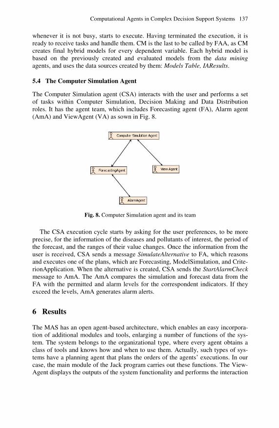
Computational Agents in Complex Decision Support Systems 137
whenever it is not busy, starts to execute. Having terminated the execution, it is ready to receive tasks and handle them. CM is the last to be called by FAA, as CM creates final hybrid models for every dependent variable. Each hybrid model is based on the previously created and evaluated models from the data mining agents, and uses the data sources created by them: Models Table, IAResults.
5.4 The Computer Simulation Agent
The Computer Simulation agent (CSA) interacts with the user and performs a set of tasks within Computer Simulation, Decision Making and Data Distribution roles. It has the agent team, which includes Forecasting agent (FA), Alarm agent (AmA) and ViewAgent (VA) as sown in Fig. 8.
Fig. 8. Computer Simulation agent and its team
The CSA execution cycle starts by asking for the user preferences, to be more precise, for the information of the diseases and pollutants of interest, the period of the forecast, and the ranges of their value changes. Once the information from the user is received, CSA sends a message SimulateAlternative to FA, which reasons and executes one of the plans, which are Forecasting, ModelSimulation, and Crite-rionApplication. When the alternative is created, CSA sends the StartAlarmCheck message to AmA. The AmA compares the simulation and forecast data from the FA with the permitted and alarm levels for the correspondent indicators. If they exceed the levels, AmA generates alarm alerts.
6 Results
The MAS has an open agent-based architecture, which enables an easy incorpora-tion of additional modules and tools, enlarging a number of functions of the sys-tem. The system belongs to the organizational type, where every agent obtains a class of tools and knows how and when to use them. Actually, such types of sys-tems have a planning agent that plans the orders of the agents’ executions. In our case, the main module of the Jack program carries out these functions. The View-Agent displays the outputs of the system functionality and performs the interaction

138 A. Fernández-Caballero and M.V. Sokolova
with the system user. As the system is autonomous and all the calculations are executed by it, the user has only access to the result outputs and the simulation window. He/she can review the results of impact assessment, modeling and fore-casting and try to simulate tendencies by changing the values of the pollutants.
To evaluate the impact of environmental parameters upon human health in the Spanish region Castilla-La Mancha, in general, and in the city of Albacete in par-ticular, we have collected retrospective data since year 1989, using open informa-tion resources offered by the Spanish Institute of Statistics and by the Institute of Statistics of Castilla-La Mancha. As indicators of human health and the influenc-ing factors of environment, which can cause negative effect upon the noted above indicators of human health, the factors described in Table 2 were taken.
Table 2. Diseases and pollutants studied in research
Type of Dis-ease/Pollutant
Disease class
Endogenous diseases:
Certain conditions originating in the prenatal period; Congenital malformations, deformations and chromosomal abnormalities.
Exogenous diseases:
Certain infectious and parasitic diseases; Neoplasm; Diseases of the blood and blood- forming organs and certain disorders involving the immune mechanism; Endocrine, nutritional and metabolic diseases; Mental and behavioral disorders; Diseases of the nervous system; Diseases of the eye and adnexa; Diseases of the ear and mastoid process; Diseases of the circulatory system; Diseases of the respiratory system; Diseases of the digestive system; Diseases of the skin and subcutaneous tissue; Diseases of the musculoskeletal system and connective tissue; Diseases of the genitourinary sys-tem; Pregnancy, childbirth and the puerperium; Symptoms, signs and abnormal clinical and laboratory findings, not elsewhere classified; External causes of morbidity and mortality.
Transport: Number of Lorries, Buses, Autos, Tractors, Motorcycles, Others;
The MAS has recovered data from plain files, which contained the information
about the factors of interest and pollutants, and fused in agreement with the ontol-ogy of the problem area. It has supposed some necessary changes of data proper-ties (scalability, etc.) and their pre-processing. After these procedures, the number of pollutants valid for further processing has decreased from 65 to 52. This significant change was caused by many blanks related to several time series, as some factors have started to be registered recently. After considering this as an important drawback, it was not possible to include them into the analysis. The human health indicators, being more homogeneous, have been fused and cleared successfully.
The impact assessment has shown the dependencies between water characteris-tics and neoplasm, complications of pregnancy, childbirth and congenital malfor-mations, deformations and chromosomal abnormalities. Part of Table 3 shows that within the most important factors apart from water pollutants, there are indicators of petroleum usage, mines outcome products and some types of wastes.

Computational Agents in Complex Decision Support Systems 139
Table 3. Part of the table with the outputs of impact assessment
Disease Class Pollutant, which influence upon the disease Neoplasm Nitrites in water; Miner products; DBO5; Dangerous chemical
wastes; Fuel-oil; Petroleum liquid gases; Water: solids in suspension; Asphalts; Non-dangerous chemical wastes;
Diseases of the blood and blood- forming organs, the immune mechanism
DBO5; Miner products; Fuel-oil; Nitrites in water; Dangerous wastes of paper industry; Water: solids in suspension; Dan-gerous metallic wastes
Pregnancy, childbirth and the puerperium
Kerosene; Petroleum; Petroleum autos; Petroleum liquid gases; Gasohol; Fuel-oil; Asphalts; Water: DQO; DBO5; Solids in suspension; Nitrites.
Certain conditions originating in the prenatal period
Non-dangerous wastes: general wastes; mineral, constriction, textile, organic, metal. Dangerous oil wastes.
Congenital malforma-tions, deformations and chromosomal abnormalities
Gasohol; Fuel-oil; DQO in water; Producing asphalts; Petro-leum; Petroleum autos; Kerosene; Petroleum liquid gases; DBO5 in water; Solids in suspension and Nitrites.
The MAS has a wide range of methods and tools for modeling, including re-
gression, neural networks, GMDH, and hybrid models. The function approxima-tion agent selected the best models, which were: simple regression – 4381 models; multiple regression – 24 models; neural networks – 1329 models; GMDH – 2435 models. The selected models were included into the committee machines. We have forecasted diseases and pollutants values for the period of four years, with a six month step, and visualized their tendencies, which, in common, and in agree-ment with the created models, are going to overcome the critical levels. Control under the “significant” factors, which cause impact upon health indicators, could lead to decrease of some types of diseases.
As a result, the MAS provides all the necessary steps for standard decision making procedure by using intelligent computational agents. The levels of the system architecture, logically and functionally connected, have been presented. Real-time interaction with the user provides a range of possibilities in choosing one course of action from among several alternatives, which are generated by the system through guided data mining and computer simulation. The system is aimed to regular usage for adequate and effective management by responsible municipal and state government authorities.
We used as well traditional data mining techniques, as other hybrid and specific methods, with respect to data nature (incomplete data, short data sets, etc.). Com-bination of different tools enabled us to gain in quality and precision of the reached models, and, hence, in recommendations, which are based on these mod-els. Received dependencies of interconnections and associations between the fac-tors and dependent variables helps to correct recommendations and avoid errors.
To conclude, it is necessary to about our future plans regarding the work. As the work appeared to be very time consuming during the modeling, we are looking

140 A. Fernández-Caballero and M.V. Sokolova
forward to both revise and improve the system and deepen our research. Third, we consider making more experiments varying the overall data structure and trying to apply the system to other but similar application fields.
7 Conclusions and Future Work
Agent-based decision making is a complicated problem, especially for a general issue as environmental impact upon human health. Though supposing it to be a tractable problem, we should note some essential advantages we have reached, and some directions for future research. Consequently, our future work can be drawn on various levels.
First, the MAS supports decision makers in choosing the behaviour line (set of actions) in general case, which is potentially difficult to analyse and foresee. As for any complex system, MAS allows pattern predictions, and the decision maker’s choice is to be decisive. The framework we have created provides flows of works for decision generation, receiving raw data which are treated by agent teams, and transforming them into knowledge
Second, in spite of our time consuming modelling work, we are looking for-ward to both revise and improve the system and deepen our research. We are planning to refine data mining methods and modify some of them, to add some new ones, which can be especially valuable for concrete works, for example, some methods to work with qualitative information, fuzzy-based methods, dimension reduction methods, etc.
Third, as the system architecture has a general structure, we consider making more experiments varying data structure, and trying to apply the system to other application fields.
Acknowledgements
This work was partially supported by Spanish Ministerio de Ciencia e Innovación TIN2007-67586-C02 and TIN2010-20845-C03 grants, and by Junta de Comuni-dades de Castilla-La Mancha PII2I09-0069-0994 and PEII09-0054-9581 grants.
References
1. Sokolova, M., Fernández-Caballero, A.: A multi-agent architecture for environmental impact assessment: Information fusion, data mining and decision making. In: 9th In-ternational Conference on Enterprise Information Systems, ICEIS 2007, vol. AIDSS, pp. 219–224 (2007)
2. Chang, C.L.: A study of applying data mining to early intervention for developmen-tally-delayed children. Expert Systems with Applications 33(2), 407–412 (2006)
3. Gorodetsky, V., Karsaeyv, O., Samoilov, V.: Multi-agent and data mining technolo-gies for situation assessment in security-related applications. Advances in Soft Com-puting, 411–422 (2005)

Computational Agents in Complex Decision Support Systems 141
4. Sokolova, M., Fernández-Caballero, A.: Modeling and implementing an agent-based environmental health impact decision support system. Expert Systems with Applica-tions 36(2), 2603–2614 (2009)
5. Bradshaw, J.M.: Software Agents. The MIT Press, Cambridge (1997) 6. Weiss, G.: Multiagent Systems: A Modern Approach to Distributed Artificial Intelli-
gence. The MIT Press, Cambridge (2000) 7. Bonczek, R.H., Holsapple, C.W., Whinston, A.B.: The evolving roles of models in de-
cision support systems. Decision Sciences 11(2), 337–356 (1980) 8. Keen, P.G.W.: Adaptive design for decision support systems. ACM SIGMIS Data-
base 12(1-2), 15–25 (1980) 9. Sprague, R.H., Carlson, E.D.: Building Effective Decision Support Systems. Prentice-
Hall, Englewood Cliffs (1982) 10. Levin, M.S.: Composite Systems Decisions. Decision Engineering. Springer, Heidel-
berg (2006) 11. Power, D.J.: Decision support systems: concepts and resources for managers. Quorum
Books, Westport (2002) 12. Chen, H., Bell, M.: Instrumented city database analysts using multi-agents. Transpor-
tation Research, Part C 10, 419–432 (2002) 13. Sokolova, M.V., Fernández-Caballero, A.: An agent-based decision support system for
ecological-medical situation analysis. In: Mira, J., Álvarez, J.R. (eds.) IWINAC 2007. LNCS, vol. 4528, pp. 511–520. Springer, Heidelberg (2007)
14. Urbani, D., Delhom, M.: Water management policy selection using a decision support system based on a multi-agent system. In: Bandini, S., Manzoni, S. (eds.) AI*IA 2005. LNCS (LNAI), vol. 3673, pp. 466–469. Springer, Heidelberg (2005)
15. de Wolf, T., Holvoet, T.: Towards a full life-cycle methodology for engineering decen-tralised multi-agent systems. In: The Fourth International Workshop on Agent-Oriented Methodologies, pp. 1–12 (2005)
16. Vasconcelos, W.W., Robertson, D.S., Agusti, J., Sierra, C., Wooldridge, M., Parsons, S., Walton, C., Sabater, J.: A lifecycle for models of large multi-agent systems. In: Wooldridge, M.J., Weiß, G., Ciancarini, P. (eds.) AOSE 2001. LNCS, vol. 2222, pp. 297–318. Springer, Heidelberg (2001)
17. Bellifemine, F., Poggi, A., Rimassa, G.: Jade – A FIPA-compliant agent framework. Practical Applications of Intelligent Agents, 97–108 (1999)
18. Repast home page (2003), http://repast.sourceforge.net 19. Schelfthout, K., Holvoet, T.: ObjectPlaces: an environment for situated multi-agent
systems. In: Third International Joint Conference on Autonomous Agents and Multi-agent Systems, pp. 1500–1501 (2004)
20. ISO/IEC 12207 home page, http://www.iso.org/iso/ 21. Guarino, N., Giaretta, P.: Ontologies and knowledge bases: Towards a terminological
clarification. In: Towards Very Large Knowledge Bases, pp. 25–32. IOS Press, Am-sterdam (1995)
22. Samoylov, V., Gorodetsky, V.: Ontology issue in multi-agent distributed learning. In: Gorodetsky, V., Liu, J., Skormin, V.A. (eds.) AIS-ADM 2005. LNCS (LNAI), vol. 3505, pp. 215–230. Springer, Heidelberg (2005)
23. DeLoach, S.A., Wood, M.F., Sparkman, C.H.: Multiagent systems engineering. Inter-national Journal of Software Engineering and Knowledge Engineering 11, 231–258 (2001)

142 A. Fernández-Caballero and M.V. Sokolova
24. Wooldridge, M., Jennings, N.R., Kinny, D.: The Gaia methodology for agent-oriented analysis and design. Journal of Autonomous Agents and Multi-Agent Systems 3, 285–312 (2000)
25. Bauer, B., Müller, J.P., Odell, J.: Agent UML: a formalism for specifying multiagent software systems. International Journal of Software Engineering and Knowledge En-gineering 11(3), 207–230 (2001)
26. Padgham, L., Winikoff, M.: Prometheus: A pragmatic methodology for engineering intelligent agents. In: Workshop on Agent Oriented Methodologies (Object-Oriented Programming, Systems, Languages, and Applications), pp. 97–108 (2002)
27. Giunchiglia, F., Mylopoulos, J., Perini, A.: The Tropos software development method-ology: Processes, models and diagrams. In: Giunchiglia, F., Odell, J.J., Weiss, G. (eds.) AOSE 2002. LNCS, vol. 2585, pp. 162–173. Springer, Heidelberg (2002)
28. Gascueña, J.M., Fernández-Caballero, A.: Prometheus and INGENIAS agent method-ologies: A complementary approach. In: Luck, M., Gomez-Sanz, J.J. (eds.) Agent-Oriented Software Engineering IX. LNCS, vol. 5386, pp. 131–144. Springer, Heidel-berg (2009)
29. Bergenti, F., Gleizes, M.P., Zambonelli, F.: Methodologies and Software Engineering for Agent Systems: The Agent-Oriented Software Engineering Handbook. Springer, Heidelberg (2004)
30. Padgham, L., Winikoff, M.: Developing Intelligent Agent Systems: A Practical Guide. John Wiley & Sons, Chichester (2004)
31. Russell, S., Norvig, P.: Artificial Intelligence: A Modern Approach. Prentice-Hall, Englewood Cliffs (1995)
32. van Lamsweerde, A.: Goal-oriented requirements engineering: A guides tour. In: 5th IEEE International Symposium on Requirements Engineering, RE 2001, pp. 249–263 (2001)
33. Liu, L., Yu, E.: From requirements to architectural design: Using goals and scenarios. In: ICSE 2001 Workshop: From Software Requirements to Architectures, STRAW 2001, pp. 22–30 (2001)
34. JackTM Intelligent Agents home page, http://www.agent-software.com/shared/home/
35. Prometheus Design Tool home page, http://www.cs.rmit.edu.au/agents/pdt/
36. Gorodetsky, V., Karsaev, O., Konushy, V., Mirgaliev, A., Rodionov, I., Yustchenko, S.: MASDK software tool and technology supported. In: International Conference on Integration of Knowledge Intensive Multi-Agent Systems, pp. 528–533 (2005)
37. ISO 14031:1999. Environmental management - Environmental performance -Guidelines, http://www.iso.org/
38. International Classification of Diseases (ICD), http://www.who.int/classifications/icd/en/

L.C. Jain and C.P. Lim (Eds.): Handbook on Decision Making, ISRL 4, pp. 143–162. springerlink.com © Springer-Verlag Berlin Heidelberg 2010
Chapter 6
A Multi-criteria Decision-Support Approach to Sustainable Rural Energy in Developing
Countries
Judith A. Cherni* and Nicole Kalas
Centre for Energy Policy and Technology, Centre for Environmental Policy, Imperial College London, 3rd Floor Mech’ Eng’ Building,
South Kensington Campus, London SW7 2AZ, UK [email protected]
Centre for Environmental Policy, Imperial College London, 3rd Floor Mech’ Eng’ Building, South Kensington Campus, London SW7 2AZ, UK
Numerous models have been developed to aid in the decision making process to identify the most suitable energy provision options for a given community or area. Some models focus strictly on one key planning aspect, such as cost or technology (single-criteria decision analysis), while other models take multiple criteria into consideration, such as cost and technology, social, human and environmental factors (multi-criteria analysis). This chapter aims to show that the inclusion of multiple technical and non-technical criteria can lead to more sustainable development outcomes. To do so, it provides a comparison between several single factor and multi-criteria models, highlighting their applications and limitations in the context of rural energy planning in developing countries. This is followed by a discussion of the factors that should be considered to ensure optimal service provision,, long-term sustainability of rural electrification projects and poverty alleviation. The subsequent section introduces and analyses the components of the Sustainable Rural Energy Decision Support System (SURE-DSS) approach and methodology. The novelty of the SURE tool lies in its objective to match rural community’s energy needs in developing countries to appropriate technologies and thereby improve livelihoods and project sustainability. The chapter explains the approach and illustrates the tool’s application through a case study in Colombia.
1 Introduction
Access to electricity is still limited despite the substantial large-scale power-grid expansion that took place during the 1960s to 1980s in developing countries. Most of the approximately 1.6 billion people (World Bank, 2006) who lack access to * Corresponding author.

144 J.A. Cherni and Nicole Kalas
electricity are located in the rural areas of the developing world (Sebitosi and Pillay, 2005). While off-grid, particularly renewable, energy technologies are often the only viable option for remote locations, many installations in rural areas have stopped functioning at the end of the project cycle (Cherni et al., 2007). A number of factors have contributed to such failures, including inadequate technical information, the lack of sustained financial resources, and capacity limitations at the local level to maintain equipments. To a significant degree, these failures stem from the unsuitable selection of appropriate energy technologies.
All too often, financial and technical criteria have dominated the choice of energy technologies at the cost of a more comprehensive and sustainable energy development framework (see, e.g., Roseland, 2000; Huang et al. 1995; Srivastava and Rehman, 2006). If the provision of energy is based solely on technical and financial parameters, solutions are likely to prove unsustainable and hence provide little support in terms of poverty reduction (Cherni et al., 2007). The trade-offs of single criteria approaches to energy planning imply that improvements in a single asset of a community (e.g., technology) may be achieved at the expense of another asset (e.g., environment) (Pohekar and Ramachandran, 2004). These concerns and limitations have motivated the design of the multi-criteria decision support system (SURE-DSS) presented here. The model’s objective is to identify and promote effective and sustainable energy solutions through the consideration of technical and non-technical dimensions of rural infrastructure through the application of a multi-criteria methodology and an inbuilt assurance mechanism aimed at improving the decision-making processes.
To date, a considerable number of single- and multi-criteria energy optimisation models have been developed to aid decision-making for modern energy applications at a national, regional or local level, including the electrification of rural areas in developing countries. Single-criterion optimization approaches applied to rural energy schemes have been described by Løken (2007), Georgopoulou et al. (1997), Kablan (1997), and Pelet et al. (2005). A main drawback of single-criterion decision-making is that physical and socio-economic conditions of prospective technology users may be overlooked (Nigim et al, 2004; Huang et al, 1995). Similarly, various forms of multi-criteria conceptualisation and frameworks have been used for the planning prioritisation of energy supply alternatives in isolated areas, including models that consider environmental impacts (Huang et al, 1995; Kablan, 1997; Beccalli et al, 1998; Hobbs and Meier, 2000; Mladineo et al., 1987; Georgopoulou et al, 2003). They also comprise multi-criteria optimization and simulation decision support systems such as LEAP (Long Range Energy Alternatives Planning), MARKAL (MARKet ALlocation) and HOMER.
While these decision tools have been crucial for supporting the development of off-grid and interconnected power systems, this chapter argues that important limitations still remain in relation to the i. geographical scale of the application; ii. participation of rural community in decision-making (Beer and Swanepole, 1994; Sebitosi and Pillay, 2005); iii. narrow number of sustainability dimensions encompassed (Limmeechokchaia and Chawana, 2007); iv. replicability of the same solutions (Roseland, 2000); and, significantly, v. the overall impact of modern energy on peoples’ livelihoods. Further, there is recognition that while modern energy provision

A multi-criteria decision-support approach to sustainable rural energy 145
may facilitate development, it may also have a negative impact on the environment or drain scarce financial resources, all of which could be mitigated if a technology solution were selected more carefully. These issues are considered below.
The first section of this chapter highlights the differences between single and multi-criteria approaches – giving more extensive consideration to the latter - in the context of sustainable rural energy planning in developing countries. To make the case for a multi-criteria approach to decision making, this discussion is followed by a brief presentation of several established models. The chapter then looks at the SURE-DSS model in detail and reports the outcome of the application of SURE-DSS in a remote Colombian rural community where total energy demands were met only partially through a diesel generator.
2 Comparing Single and Multi-criteria Energy Decision Support Systems
Two main approaches can be distinguished in energy decision-making, single-criterion and multi-criteria methods. This section summarises the main characteristics of these methodologies.
Single-criterion models consider one key planning aspect only, such as cost or technology, and have been used widely in the development of rural energy schemes (e.g., Løken, 2007; Georgopoulou et al., 1997; Kablan, 1997; Pelet et al., 2005). A main drawback of single-criterion decision-making is that physical, socio-economic, and/or environmental conditions of prospective technology users are overlooked (Nigim et al, 2004; Huang et al, 1995). Often, improvements in a single asset may lead to the deterioration of another asset (Pohekar and Ramachandran, 2004). For example, when technological and economic considerations dominate during service expansion (Mirasgedis and Diakoulaki, 1997; Georgopoulou et al., 1997), considerations such as income generation potentials and the effect on the environment are often sidelined (as observed during the rural electrification of the 1960s to 1980s).
RET Finance and e-analysis are two examples of single-criteria DSS that have been used to analyse the costs of proposed energy projects. Both were developed by the U.S. National Renewable Energy Laboratory (NREL). Renewable Energy Technology Financial Model (RET Finance) is a renewable energy technology (RET) finance model used to calculate energy costs of RETs such as biomass, geothermal, solar, and wind. It is a levelised cost-of-energy model which simulates a detailed 20-year nominal dollar cash flow for renewable energy projects, including earnings, cash flows, and debt payment to calculate a project's cost-of-electricity, after-tax nominal Internal Rate of Return, and annual Debt-Service-Coverage-Ratios. The e-analysis model allows the planner to conduct a real options valuation of renewable energy research and development (R&D) and distributed generation assets (NREL).
If the provision of energy services is addressed from solely from technical or financial perspectives, and planners neglect to consider a more encompassing sustainable energy development conceptual framework (see, e.g., Roseland, 2000;

146 J.A. Cherni and Nicole Kalas
Huang et al. 1995; Srivastava and Rehman, 2006), solutions are likely to remain unsustainable and hence give little support to poverty reduction (Cherni et al., 2005; 2007). However, it should be emphasised that these models can be very useful if applied to very specific purposes, or when complemented by additional tools.
The second approach, multi-criteria decision analysis (MCDA), provides a framework for the assessment of various alternatives and thus considers more than one planning aspect in the design of policies and development projects. The growing need to incorporate environmental considerations into energy planning in the 1980s accelerated the use of multi-criteria approaches (Georgopoulou et al., 1997). A multi-criteria analysis is useful and necessary, as the prioritisation of electricity generation options is a multi-faceted problem requiring consideration of qualitative and quantitative, as well as technical and non-technical factors. In approaching the planning of energy provision in rural areas, conventional tools and assessment methods generally emphasis three key decision-making aspects, which may be classified as the technological, economic, social and the environmental approach (Cherni et al., 2007).
The chief objective of the technological category has been to maximise the supply of energy. An analysis of various technological factors may take into account the type of proposed energy solution (conventional and/or renewable energy technologies); its efficiency and suitability in terms of meeting energy demands (Georgopoulou et al., 1997); the maturity of the energy technology considered (Beccali et al., 1998); its applicability (Georgopoulou et al., 2003); its dependence of fossil fuels (Kablan, 1997) and the availability of required fuel resources (Borroto et al., 1998); and the disadvantages and uncertainties related to the construction process of a power generation facility (Angel y Smith, 2000), among others. Additional technical criteria considered may be the state of art of technologies in terms of their application and conditions under which they were employed; the technical resources of a site, such as wind speed, solar radiation, and availability of biomass; operating characteristics, including local capacity to operate and maintain the systems; and level of local replicability (Biswas et al., 2001).
An example of a technology-centred model is the Hybrid Power System Simulation Model (Hybrid2). The tool was developed by the Renewable Energy Research Laboratory (RERL) at the University of Massachusetts at Amherst, simulates the performance of various wind, photovoltaic, and diesel hybrids, and provides comparisons of the long-term performance of similar systems. Hybrid2 can be used to conduct detailed long-term performance and economic analysis on a wide variety of hybrid power systems.
In contrast, the main goal of the economic approach has been to minimise the financial costs associated with an energy project (e.g., Smith et al., 2000; Georgopoulou et al., 1997; Koroneos et al., 2005). Indicators employed in an economic analysis may include: investment cost (Kablan, 1997); cost per unit of both installation and generation (Angel and Smith, 2000; Polatidis and Haralambopoulos, 2002); operation and maintenance costs (Watson and Ter-Gazarian, 1999); fuel costs (Kolhe et al., 2002) and available resource costs (Kablan, 1997); the internal rate of return (Angel and Smith, 2000); greenhouse gas emission reduction costs (Georgopoulou et al., 1997, 2003) – or credits; job

A multi-criteria decision-support approach to sustainable rural energy 147
creation attributable to the project (Borroto et al., 1998); and others (Cherni et al., 2007). For example, the model developed by Biswas et al. includes the condition that RETs be financially feasible and sustainable through household income generation and follow-on monitoring and on-site maintenance services (2001).
An illustrative example of a model that aims to minimise overall costs is VIPOR. VIPOR is a computational tool capable of designing an autonomous village electrification system using the lowest cost combination of centralized and isolated generation. Based on information on the local terrain, village layout and size, load sizes and equipment costs, the model determines which houses should be powered by isolated power systems (e.g., solar home systems) and which should be included in a centralized distribution grid. Another example is Energy10, which has been designed by NREL to identify the most cost-effective combination of energy-efficiency strategies and energy-saving measures for small commercial and residential buildings, such as day lighting, passive solar heating, and high-efficiency mechanical systems (NREL).
The focus of the social approach has been to maximise welfare impacts (Beccali et al., 1998). For example, Georgopoulou et al., (1997) consider social criteria as a macro-objective which is 50% political (e.g., cohesion among local activities and regional employment) and 50% environmental (e.g., air quality, noise, visual amenity, among others). Borroto et al. (1998) suggest that the social criteria should be drawn on actual constrains, such as the achievement of annual rural energy demand. Specific criteria may include social equitability and cultural appropriateness, generation of employment, and institutional capacity development (including enabling energy pricing policies and tax system, laws and energy product standards) (Biswas et al., 2001).
The main focus of the environmental approach, on the other hand, has been the attempt to mitigate anticipated environmental damages (Mirasgedis and Diakoulaki, 1997; Georgopoulou et al., 2003, Huang et al, 1995; Kablan, 1997; Beccalli et al., 1998; Hobbs and Meier, 2000; Mladineo et al., 1987; 2003). Cherni et al. point out that few DSS models employ indexes to account for environmental impacts, such as a greenhouse gas emission (Beccali et al., 1998; Borroto et al., 1998; Georgopoulou et al., 2003) or deforestation index (Kablan, 1997); an index of the minimum land area required by a particular energy technology (Beccali et al., 1998; Georgopoulou et al., 1997); noise level (Georgopoulou et al., 1997), water, air, and soil quality indices,among others (2007).
In addition to the aforementioned tools, Jebaraj and Iniyan provide a detailed description of a number of more integrated energy planning, supply-demand, forecasting and optimisation models (2006). The case studies for these DSS models are largely situated in India and represent various scales, i.e., farm/household levels, clusters of households, and regional. Apart from looking at technical, economic or environmental criteria, the authors distinguished the following types of models: energy planning, energy supply-demand, forecasting, renewable energy, emission reduction, and optimisation models (2006). In his analysis of energy planning decision support systems (DSS), Løken divides MCDA models into three different categories: value measurement models; goal, aspiration and reference level models; and outranking models (2007).

148 J.A. Cherni and Nicole Kalas
In addition to the careful consideration of multiple criteria, a DSS’s applicability also depends largely on the scale employed and the level of aggregation of the data. These need to be matched carefully to the type and size of project. Typically, energy planning is conducted at the following levels: household, village; regional; national; and international. An example of a regional scale model is the City-cluster Energy Systems Planning Model (CCEM), which can be applied to multiple cities within a region. The model accounts for environmental emissions, technology options, policy consideration, costs, demography, environment and sociology. CCEM was used in the Toronto-Niagara Region for ’optimizing’ energy production based on a least-cost strategy, assessing environmental emissions by source, and exploring economic and environmental consequences of different policies (Lin et al., 2009)”.
Multi-criteria approaches to energy planning have yet to overcome a number of limitations. For example, policy decision-making still tends to privilege technical criteria and quantitative information, i.e., power output and costs. Thus, the technical features of technology expansion tend to prevail in the models and decision-makers’ minds rather than other valid priorities, such as social wellbeing.
After reviewing the main characteristics of single- and multi-criteria approaches, the chapter looks now into few specific energy models to illustrate their possible applications.
3 Reach and Limitations of Energy Multi-criteria DSS
Multi-criteria analysis has been employed to support decision-making in the context of rural energy provision in the developing world with the objective to either replace existing technologies (e.g., wood burning for heating and cooking), or to implement new ones (see e.g. Huang et al., 1995; Kablan, 1997; Beccali et al., 1998; Watson and Ter-Gazarian, 1996; Hobbs and Meier, 2000) while mitigating environmental impacts (Georgopoulou et al., 2003; Borroto et al., 1998).
This section analyses select multi-criteria energy planning models, provides examples of their application and highlights their strengths and limitations. This is not meant to be a comprehensive summary, but rather an illustration of the extent to which a few, often used models may refer to the criteria discussed above. Each description includes the name of the model, the underlying methodology, and, if available, examples of their practical application.
HOMER, a widely applied optimisation model developed by the USA National Renewable Energy Laboratory (NREL, 2003), assists in the evaluation of power distribution for both off-grid, remote, stand-alone generation applications and grid-connected systems. It is a useful tool and has been employed in a number of developing countries with good results. However, HOMER judges outcomes based upon two criteria only, their economic and technical merits, and while these are crucial aspects of any off-grid energy system, the model has not been designed to evaluate such significant impacts as the social and environmental.
The Long Range Energy Alternatives Planning (LEAP) is also a scenario-based energy-environment modelling tool. The scenarios considered are based on comprehensive accounting of how energy is produced, converted and consumed in a given region or economy under a range of alternative assumptions on

A multi-criteria decision-support approach to sustainable rural energy 149
population, economic development, technology, and price. In contrast to HOMER, LEAP has been applied at multiple spatial levels including local rural areas, large metropolitan cities, and at the national, regional and global level (SEI).
MARKAL (MARKet Allocation) is a well-established linear programming tool that minimises provision costs under several constraints, including energy demand; it has been used predominantly in a large-scale electricity development context (Cherni et al. (2007). The model integrates energy, environmental, and economic factors to inform energy policy and to support national energy planning decision-making. MARKAL proposes a set of technology options that minimise cost, while meeting consumer demands and considering environmental impacts (BNL).
The ELECTRE is another widely used methodology that was developed by Bernard Roy in the 1970s and applies an outranking approach with specified thresholds to solve real-life problems (Roy, 1991). More recently, ELECTRE has been adapted to energy planning. For example, Beccali et al. devised a model based on ELECTRE to analyse option for the diffusion of RETs at a regional level. The multi-criteria methodology employed by their model allows decision-makers to assess various innovative energy options and choose the most appropriate set based on pre-determined objectives (2003).
Additional models were developed with the aim to assist decision-making in rather specific energy planning situations, e.g., monitoring of household energy use (SAVE, see Boonekam, 1997; FACE, see Messner and Strubegger, 1987; Lutzenhiser, 1992; Reddy, 1995; FORECAST, FORCEE, see Kimmins, 1997).
Finally, a number of models based on the integrated renewable energy system (IRES) were developed and applied to rural electrification efforts in India, Nepal and Bangladesh (Akella et al., 2007). The models helped to determine the most appropriate renewable energy options – or a combination of various RETs – for specific household applications and communities in these rural areas.
More recently, Terrados et al. proposed a “hybrid’’ methodology for renewable energy planning at a regional level based on lessons learned from existing multi-criteria decision analysis models, the Strengths-Weaknesses-Opportunities-Threats (SWOT) analysis, and expert opinion ‘‘Delphi’’ methods. The model proposes the following steps: “1) Initial diagnosis of regional energy system; 2) Diagnosis configuration as SWOT matrix; 3) Initial selection of strategies through SWOT analysis; 4) Validation and assessment of strategies by means of experts opinion; 5) Ranking of alternatives applying MCDA; 6) Reference plans analysis; and 7) Final strategies selection and targets establishment”(2009). The SWOT approach, as the SURE-DSS methodology, entails an iterative process which incorporates experts’ opinion at various stages. Table 1 provides a comparison of the models mentioned above in terms of their determining criteria.
While these tools have fulfilled a role in supporting decisions to promote off-grid and interconnected power systems, limitations remain in terms of the scale its application, i.e., these might be too broad or too specific, limited to community involvement in decision-making (Beer and Swanepole, 1994; Sebitosi and Pillay, 2005), poor considerations of sustainability issues, and the chances of replicability of solutions are too slim (Roseland, 2000; TERI, 2003).

150 J.A. Cherni and Nicole Kalas
Table 1. Main analytical criteria found in select energy planning models
Furthermore, multi-criteria methods have thus far failed to measure adequately
the sustainability of an energy option, i.e., the likely improvement of a community’s assets over the longer term resulting from the effective application of the selected technology. Consequently, the implemented solutions have largely neglected sustainability and poverty reduction concerns (Cherni et al., 2007).
Criteria
Model Economic Technical Social Human Environmental Scale(s) *
Single-criterion models
RET Finance
e-analysis
Multi-criteria models
HOMER H?, V, R
Hybrid2
VIPOR V
Energy10 H
LEAP V, R, N
IRES
Biswas et al. ?
MARKAL N
IRES
ELECTRE ? R
CCEM R
SWOT &
Delphi R
* Scales: H – household; V – village; R – region; N – national; I – international

A multi-criteria decision-support approach to sustainable rural energy 151
As mentioned above, the failures of installed off-grid rural energy systems can be largely traced to decisions either based on political, financial and environmental criteria, but without adequate consideration for the overall sustainability of the infrastructure development (see, e.g., Roseland, 2000; Polatidis and Haralambopoulos, 2002; Huang et al 1995; Omer, 2006; Srivastava and Rehman, 2006) or a communities’ preferences and expressed needs (see, e.g., Beer and Swanepole, 1994; Sebitosi and Pillay, 2005).
Similarly, Santos and Linares noted that an important factor in the unsuccessful provision of effective energy technology projects is the failure to identify explicitly the target users’ wishes, needs and strengths (2003). In fact, current methods often allow the population to participate only after the experts have made the technical decisions. Yet, it has been claimed that it is desirable, if not vital, for both planning and assessment to encourage the participation of those on whom the given energy interventions will affect most, rural individuals and households (see Bannister, 2002; Barnes, 2000; Barnett, 2000).
Increasingly, though, rural energy experts have come to appreciate that in order to succeed, energy projects must involve the local community from the very beginning, prioritising their input and harnessing their interest, support and investment (e.g., Kartha and Leach, 2001). This is a considerable advance compared to the purely technocratic approaches of previous decades. Participatory methods aim to learn from rural individuals what the status quo is in their communities and how their existence might best be improved through external assistance.
These concerns and the identified limitations of existing approaches have motivated the design of the decision support approach and methodology SURE-DSS (Sustainable Renewable Energy Decision Support System) to promote effective and sustainable energy solutions, combine technical and non-technical criteria for the development of rural infrastructure, to design participatory methods and include an inbuilt assurance mechanism to improve the decision-making processes.
4 SURE-DSS: A Comprehensive Multi-criteria Approach and Application
While there is recognition that modern energy may facilitate development, and could be critical for the achievement of the Millennium Development Goals (MDG) (DFID, 2002), some energy technologies may also have a negative impact on the environment or place a drain on already scarce financial resources. By considering a wider range of factors and potentially positive and negative impacts, a multi-criteria approach is better equipped to in the selection of technologies with a more benign ecological footprint or less adverse socio-economic impact. Yet, the selection of technologies to supply energy to the rural poor in developing countries to improve their livelihoods is a particularly complex activity. The Sustainable Renewable Energy Decision Support System (SURE-DSS) was designed with the objective to aid and enhance the decision-making process to

152 J.A. Cherni and Nicole Kalas
achieve sustainable and affordable supply of energy in rural poor areas, many of which may also be remotely located.
SURE-DSS is a methodological software package designed to fill the present gap in the planning of future energy development that is both technologically appropriate and sustainable in the long-term. It provides an optimisation assessment of various electrification scenarios and aims to assist in energy development for enhancing rural livelihoods. The model was developed by the international research project (2001-2006) Renewable Energy for Sustainable Rural Livelihoods (RESURL), funded by the UK Department for International Development (DFID). SURE-DSS is designed to aid decision-makers to define and select appropriate energy supply options in rural areas for poverty reduction and sustainability.
The SURE-DSS combines quantitative and qualitative criteria and – unlike other existing multi-criteria software that assist rural energy decision-making – the SURE approach enables the priorities of a group of prospective users to be considered in the analysis. The model draws on the concept of Sustainable Livelihoods (SL) approach, which is a particularly people-centre approach that emphasises the importance of understanding and connecting various components of livelihood. The term “sustainable” signifies that the mechanisms put into practice to enable people to ensure and enhance their livelihoods must be lasting (Ashley and Carney, 1999).
The SL approach acknowledges that a community owns five categories of assets or capitals, which can be categorised as follows: physical (e.g., houses, roads), financial (e.g., wages, savings), natural (e.g., water, land resources), social (e.g., networks and local organisations), and human (e.g., education, skills). In the SURE approach these capitals act as indicators for assessing existing conditions in a rural community, calculating the energy needs and determining overall priorities of a population, and simulating their future condition through the implementation of alternative energy systems. The SURE-DSS model attempts to facilitate decisions that promote energy infrastructures that ensure and enhance the quality of rural livelihoods permanently by paying equal attention to non-technical aspects of energy provision, such as socio-economic and environmental factors.
To achieve this, the SURE-DSS model initially assesses the strengths and weaknesses of a community by indicating its overall status of capitals or assets. It then proceeds to draw up energy plans, which would affect the community’s assets differently. The model aims to find energy solutions that would shape those assets that the potential users of the technology singled out to be in need of improvement. One particularly useful aspect of the model is that SURE-DSS uses a pentagon to illustrate the links among these five assets or capitals graphically and to show the potential changes and trade-offs associated with the implementation of different energy alternatives ‘before’ and ‘after’ an energy intervention. The graphic illustration of various energy solutions is a unique attribute of this methodology and proves particularly useful as the pentagons depict the potential changes to the baseline conditions of a household, community or, region in response to the implementation of modern energy technologies. In Eq. (1) below, Xj represents a separate set of factors for each asset function.

A multi-criteria decision-support approach to sustainable rural energy 153
),...,1;5,...,1(,1
1)(
)(nij
eAC
ijj AXij ==+
= −α (1)
Cj (Ai) represents the evaluation of the i-th energy alternative (Ai, i=1,…,n) against the resource j, j=1, 2,… 5, (1 indicates Physical, 2 Financial, 3 Natural, 4 Social and 5 Human capital); Xj (Ai) represents the effects of the i-th energy alternative on the corresponding community’s resource j; and αj is a scale parameter, associated to the number of factors that compose each resource j.
In the SURE-DSS each factor shows a range of values between 0 and 1, where 0 reflects no positive effect from energy alternative i on asset j, and 1 means a highest effect. The ideal and maximum measure of positive impact that a community may attain is therefore 1; a further measurement is given by the community baseline; and a final calculation is obtained from the impact of energy alternatives on the assets of the community.
For example, the SURE-DSS was applied in the remote rural community of San José de Cravo Norte II (SJCN II; 400 inhabitants), situated in the eastern part of Colombia in the oriental plains of Arauca (DANE, 2000). 101 households and local leaders were surveyed, and information gathered in this manner was used to build the community’s baseline and to determine the residents’ demands for electricity and other energy services. The survey revealed that only 12% of the population were supplied with electricity produced by a 5kWh diesel generator plant. Due to high operational costs and the community’s limited finances, the diesel plant only operated for 7 hours per day.
An analysis of the information obtained in the survey revealed the need for a technology solution that would provide the current health clinic with uninterrupted electricity for vaccines and medications to be safely refrigerated. Additional electricity was requested to power a communal centre. In addition to improving access to electricity, the new energy system was to increase the daily access to electricity for pumping water. Finally, energy was requested to enhance the productivity of the local dairy industry – i.e., mechanisation of livestock rearing, refrigeration and processing – which is the main economic activity in the region, and to spur the development of new enterprises.
An assessment of the extent of the five types of resources found in SJCN II – i.e., physical, financial, natural, social and human capitals – before the implementation of an additional source of electricity, highlights the weaknesses and strengths of this rural community. Using the SURE-DSS approach, it was found that the extent of resources owned by SJCN II while using a small diesel generator was below half of the potential total assets that the community could have. In SJCN II there were larger social and financial (both 0.4) than natural (0.3) and human (0.3) capitals, but these resources were higher than the physical assets (0.1) (see Table 2). These figures (i.e., all lower than 1) indicate that every asset could be improved through enhanced energy supply, if the community’s articulated priorities were congruent with the proposed energy technology options. The SURE tool calculated that SJCN II needed to generate at least an additional 40kWh if it was to fulfil the users’ demands.

154 J.A. Cherni and Nicole Kalas
Table 2. State of local assets* when using a diesel generator, SJCN II, Colombia 2003
Energy Technology Resources owned by SJCN II
Physical Financial Natural Social Human
Diesel generator plant
(5 KWH)
0.1 0.4 0.3 0.4 0.3
* Highest possible state = 1.
As mentioned above, the SURE-DSS’ “livelihood and energy pentagons” provide a visual representation of the state of development of a community and a baseline established through the participatory survey, and additional technical and observation information under real, current conditions of energy supply. It follows that the distance between a smaller and outer pentagon illustrates the extent that a community lacks in assets. In other words, the closer any edge of the small pentagon is to its centre point (i.e., = 0), the weaker the access to, or ownership of a particular asset is, and vice versa, the larger it is, the closer to the ideal figure the better off the community is. (See large and internal pentagons in Figure 1).
SURE-DSS thus enables decision-makers to evaluate the effect that new operating energy systems may have on assets owned by individuals, communities or a number of villages. It does so by calculating and comparing the initial condition of the assets in a community with values resulting from modelling the implementation of new energy alternatives. A main contribution of the system therefore is that it models: the gaps between a theoretically fully developed condition and an actual state of assets; the possible effects on such assets of particular energy technologies; and finally, it is possible to also foresee the specific trade-offs that alternative energy solutions would imply for livelihoods. The decision-support tool also calculates trade-offs which occur when one set of technologies, rather than another, is selected (see Figure 2 for possible solutions). Such trade-offs are likely where access to resources may change as a result of a specific technological intervention. For example, in the case of SJCN II, users’ financial resources would generally improve (0.5) with the implementation of different energy alternatives, with the exception of two technology options; if selected, the solar photovoltaic (0) and diesel–solar (0) options would not enhance user’s assets due to their plant and installation costs and poor performance in relation to reported demand, (for more details, see Cherni et al., 2007).
The multi-criteria SURE-DSS draws on a Compromise Programming (CP) method with metric two for decision-making and weights. For CP decision-makers preferences can be expressed as the measure of a metric distance between two alternatives in the space of objectives (Yu, 1973; Zeleny, 1973). A main reason for searching compromise solutions is that while Action A may be better than Action B according to one criterion, it might be worse according to another, consequently, compromise solutions must be sought (Munda et al., 1994) (Cherni et al., 2007).

A multi-criteria decision-support approach to sustainable rural energy 155
0.0
0.2
0.4
0.6
0.8
1.0Physical
Financial
Natural Social
Human
Current Diesel plant Ideal
*Small pentagon; Baseline Index: 0.0 to 1.0
Fig. 1. Ideal resources and baseline* pentagons with a 5 KWH diesel plant in SJCN II, Colombia 2003
As previously stated, the choice of an energy option for poor rural areas is not a simple task. However, by modelling the results through the SURE approach and using the geometric shape of pentagons makes the task more achievable. It was possible in the case SJCN II to ascertain possible changes to its baseline. By modelling the prospective impacts of a technology in a single figure, this DSS approach succeeds in avoiding the fragmentation of information that usually emerges from a table or a bar chart, (fragments of information might, nonetheless, be necessary for particular purposes). Further, the energy and livelihoods pentagons for SJCN II also show each capital individually (see Fig. 2).
Fig. 2. Possible appropriate energy technologies for SJCN II

156 J.A. Cherni and Nicole Kalas
The borders of a pentagon obtained in this way show how the total livelihoods would look like after a number of years where a particular energy technology solution had been in operation.
The various pentagons shown in Fig. 2 indicate how various technologies would affect assets in SJCN II. The shapes have been configured in relation to the framework of the optimal livelihood state for SJCN II, that is, an ideal pentagon which indicates the highest possible level of development whereby all the assets are fully and equally developed (i.e., where Capital j =1 = ; see above). While one pentagon simulates the state of livelihoods with the current diesel generator that supplies energy for 12% of the population, the other pentagons depict alternative livelihoods that may be attained with other technologies implemented.
In the case of SJCN II an optimum energy option (it pushes the capitals closer to the ideal pentagon) would be to continue using the existing diesel generator together with the addition of a micro-hydro power plant (see Table 3). The next best option is a micro-hydro plant alone, with a slightly lower score (0.9) than solution number 1. According to this analysis, the current diesel plant alone is the least recommended solution of all (0.0).
Yet, the choice of energy technology will depend in large part upon the decision-makers’ preferences which depend on acknowledgement and recognition of the priorities and financial state of prospective users, as identified during the survey. Solution 1 would generate up to 45kWh, that is, the power needed to meet the demands of SJCN II. Following this option, the current diesel plant must continue to operate and generate the 5 kWh and the additional 40kWh would be supplied by a new micro-hydro plant. The solution cost per kWh is US$ 1,024 and the total initial investment is US$ 40,960. This solution would produce electricity for at least 30 years and provide energy to between 90% and 100% of the population.
Table 3. Scores for most appropriate technology options, SJCN II, 2003
Solution
number Energy Technologies
Score of
appropriateness*
1 Diesel and micro-hydro 1.0
2 Micro-hydro 0.9
3 Diesel and Biogas 0.8
4 Biogas 0.8
5 Grid 0.8
6 Diesel-Solar 0.3
7 Solar Photovoltaic 0.1
8 Current Diesel plant 0.0
*The larger the score, the more appropriate the technology

A multi-criteria decision-support approach to sustainable rural energy 157
It was anticipated that the quality of the service would be similar to that received by beneficiaries connected to the national grid. A biogas plant in SJCN II would cost slightly less (US$ 36,000, or US$ 900 per kWh) than the micro-hydro plant, but it would not be able to satisfy all the demands. The installation of a 40kWh photovoltaic system would require an investment roughly three times larger (i.e., US$ 170,000) than that required for a new micro-hydro plant and the cost of connecting to the grid would exceed US$ 300,000, at a cost of US$ 10,000 per km of grid extension. However, if the combination of diesel and micro-hydro solution were implemented (see Figure 3), improvements would take place to the physical (+0.7), financial (+0.4) and human assets (+0.4) of SJCN II.
In terms of infrastructure or physical capital, more satisfactory energy provision means: 30 years of reliable electricity service; flexible energy service; lower dependency on fossil fuels than had they chosen to expand the existing diesel generator or connect to the grid; and provision of supply for at least 18 h per day of possible uninterrupted service to all sectors of demand. The supply would facilitate the operation of a health centre, school, houses and water supply system as requested by prospective users. Further, new energy infrastructure would an improvement to the existing financial asset. Such a change would be the outcome of both direct and indirect intervention: approximately 30 local jobs would be generated during the construction phase of the energy project and 40% more employment opportunities would arise in animal husbandry, handicrafts, business and services.
In the long term, the only resource of SJCN II that would not improve as a result of a new electricity solution is the environment. The natural capital would suffer some deterioration due not only to the new intervention in the local environment (i.e., the construction of a new micro-hydro plant) but because the diesel generator would continue to pollute the air and making noise. Moreover, a section of the river that would be used for the construction of the micro-hydro plant would be slightly damaged. It is however likely that provision of electricity from a micro-hydro grid would somewhat reduce the need for firewood. Some changes in the community social networks would occur due to the probable participation of local people in the construction phase, during use and operation, and while maintaining the micro-hydro plant. As part of enlarged social capital, a local administration committee could also be formed to manage the plant and collect electricity consumption fees.
Finally, modelling in SJCN II shows that the provision of appropriate energy technology would translate into improvements in the lives of the 400 inhabitants. For example, there would be a potential growth of 60% in education (i.e., the school could accommodate more children, while more school space as well as more teaching hours would be made available), and improved standard of health could be achieved through quality electricity service expansion.
6 Long-Term Energy Solutions
Among the other aspects that can be learnt from the application of this decision support system is that coping with the complexity of the technology— which in this case is medium—offers the opportunity to acquire new skills. The potential for

158 J.A. Cherni and Nicole Kalas
development of each asset with the provision of energy varies according to its initial state and the capacity of the technological option to provide for a particular demand.
These results also indicate that there is still a large potential for improvement of SJCN II, yet it is more likely that further changes would be achieved by the introduction of social policies that by further applications of technology energy development.
The SURE-DSS models enable the analysis of data from household surveys as well as additional technical information and in this way, it not only possible ascertains technology solutions, but importantly, it project energy technology effects on the current state of assets of a community and the possible enhancement, or otherwise, that might arise.
While improvements are likely to take place through the use of energy technology, as it was evident in the SJCN II case, it is likely that the appearance of new problems and crucial trade-offs could also emerge (i.e., slightly more environmental damage would ensue from continuing relying on diesel; less emissions would be emitted if the preferred solution were diesel and solar, or just a photovoltaic solution which would be, nonetheless, too expensive). These findings show that while energy technology might be crucial to achieve sustainable rural livelihoods, the choice of technology must be approached from a dynamic and comprehensive perspective in order to factor in its many linkages and attains its potential.
The problem which this DSS addresses involves the formulation and selection of an energy supply system that best suit the energy demands and possibilities of a community, while guaranteeing energy systems performance in the long term and enhancing local livelihoods. In this framework, this decision support system simplified the task of evaluating the different energy options that would best fit a community’ needs while maximising its resources and thereby contributing to poverty reduction. A particularly useful aspect of the SURE-DSS is that, uniquely, and unlike any other of the DSS discussed above, it incorporates current assets, actual demands and priorities of the target community and matches them to energy options.
Given that the application of a particular energy technology can lead to improvements in some dimensions while proving detrimental to others, there are certain implications that emerge from this study. E.g., quantitative monetary valuation of such trade-offs could greatly assist policy decision-making. Additionally, there is a need to expand the trade-off pentagons so as to illustrate not only how social groups within a community distribute benefits and burdens, but also how the different actors, i.e., the utility providers, the government and the community, play out.
Thus, the main advantage associated with SURE-DSS is that, in employing a multi-criteria approach based on the SL framework, it allows full consideration of the large quantity of data, relationships and objectives that are generally present in real world policy problems. Furthermore, it models the likely effects and trade-offs of projected energy solutions on various types of resources that a community might possess. In doing so, SURE-DSS enables decision-makers to look into technological options that might raise the chances of success of future energy developments in poor areas.
Finally, a main goal of this DSS is to prove that an energy system solution would be effective when, in addition to high technological and economic

A multi-criteria decision-support approach to sustainable rural energy 159
performance, it also promotes positive changes in the undertakings of other aspects of a target community. The application of the SURE-DSS is expected to assist in achieving long-term sustainable energy in rural areas. For any decision regarding rural energy option to be sustainable, it must engage with technical as much as non-technical factors, as the SURE does.
7 Conclusion
SURE can be helpful in cases when policy decision-makers attempt to carefully consider and weigh investment capacity, local requirements and existing conditions. The SURE tool system can then be used to calculate the most appropriate energy solution, that is, the one that both fulfils a population’s priorities and reduces poverty, and complies with government policy. Further, selection of the best energy options needs to measure the sustainability impact of energy technology on a community and, to do so, it is necessary to have a disaggregated view of the factors at community level that may be affected by energy development. This was achieved by framing the analysis within a SLA. A legitimate issue that needs to be taken into consideration is whether any target population will share and accept the outcomes suggested by a models like SURE.
The SURE multi-criteria sustainable livelihoods approach to decision-making can demonstrate to policy-makers how the provision of particular energy technologies may positively affect certain aspects of a community’s livelihood while negatively impacting others. It is a valuable contribution to the effort of bringing affordable, sustainable energy to poor rural communities in the developing world. This type of information and its straightforward illustration can be crucial for a community searching for feasible solutions to concrete problems as well as for national government programmes targeting sustainable rural development in specific areas. How the baseline could be changed is usually an aspect little explored in calculations by experts. This methodology, however, enabled the identification of farmers’ priorities in an uniform format.
The SURE approach represents a step forward in acknowledging the role of energy provision for poverty reduction. It also promotes solutions that are environmentally and socially sustainable in the long term. This chapter has described and systematically analysed the possible impacts of effective, affordable and clean energy on a community. The extent to which human and social resources can be enhanced when more energy is made available has been shown, as part of a new methodology to decision making.
Concepts and methods in decision support related to modern energy provision for poverty reduction in developing countries is itself a new direction. In this context, the approach of SURE is novel not only because it incorporates, in a systematic way, prospective users’ priorities, their demands and actual conditions as part of the analysis. SURE is also an essential feasibility tool because it looks at the technical, social, environmental, financial and human aspects of a energy development, rather than just few of these components. It provides a comprehensive approach and, because it draws on the principles of Sustainable Livelihoods, its objective is to achieve equality of access to all in a poor population, environmental protection and

160 J.A. Cherni and Nicole Kalas
users’ participation. The provision of affordable and efficient energy services in poor areas of developing countries may well contribute to improve the livelihoods of the 1.6 billion people worldwide who are in deep poverty and still rely on firewood or have very limited access to expensive and very polluting energy services.
References
1. Akella, A.K., Sharma, M.P., Saini, R.P.: Optimum utilization of renewable energy sources in a remote area. Renewable and Sustainable Energy Reviews 11, 894–908 (2007)
2. Angel, W., Smith, R.: Evaluación de alternativas y definición de un proyecto hidroeléctrico mediante el empleo de análisis multiobjetivo. XIX Congreso Latinoamericano de Hidra´ulica—Cordoba, 589–598 (2000)
3. Ashley, C., Carney, D.: Sustainable Livelihoods: Lessons from Early Experience. Department for International Development (DFID). Russell Press Ltd., Nottingham (1999)
4. Bannister, A.: The sustainable urban livelihoods framework—a tool for looking at the links between energy and poverty. Boiling Point (48) (2002), http://www.future-energy-solutions.com (Accessed: June 13, 2003)
5. Barnes, D.: Energy and poverty: strategies for assisting the rural and urban poor. Background paper for the World Bank energy strategy. World Bank, South Asia Region, Energy Sector Unit, Washington, DC (2000)
6. Barnett, A.: Energy and the fight against poverty (2000), http://www.livelihoods.org ( Accessed: April 14, 2003)
7. Beccali, M., Cellura, M., Ardente, D.: Decision making in energy planning: the ELECTRE multicriteria analysis approach compared to a fuzzy-sets methodology. Energy Conversion and Management 39, 1869–1881 (1998)
8. Beer, F., Swanepole, H.: Energy and the community of the poor: Urban settlements, household needs and participatory development in South Africa. Energy Policy, 145-150 (1994)
9. Biswas, W.K., Bryce, P., Diesendorf, M.: Model for empowering rural poor through renewable energy technologies in Bangladesh. Environmental Science and Policy 4(6), 333–344 (2001)
10. Borroto, B., Borroto, N., Vázquez, M.: Alternativas energéticas para el desarrollo de asentamientos rurales ambientalmente sostenibles. Energía, 71–77 (1998)
11. Brookhaven National Laboratory (BNL). MARKAL, http://www.bnl.gov/est/markal.asp
12. Cherni, J.A.: What energy systems are appropriate for poor villagers? id21 news. RESURL. Imperial College, London (2005)
13. Cherni, J.A., Dyner, I., Henao, F., Jaramillo, P., Smith, R., Font, R.O.: Energy supply for sustainable rural livelihoods. A multi-criteria decision-support system. Energy Policy 35, 1493–1504 (2007)
14. DANE, Colombian National Department of Statistics (2000), http://www.dane.gov.co

A multi-criteria decision-support approach to sustainable rural energy 161
15. Department for International Development (DFID), UK. Energy for the Poor - Underpinning the Millennium Development Goals (2002), http://www.dfid.gov.uk/Documents/publications/energyforthepoor.pdf, Department of Energy (DOE). MARKAL (MARKet ALlocation) Model, http://www.bnl.gov/est/markal.asp
16. Georgopoulou, E., Lalas, D., Papagiannakis, L.: A multicriteria decision aid approach for energy planning problems: the case of renewable energy option. European Journal of Operational Research 103, 483–500 (1997)
17. Georgopoulou, E., Sarafidis, Y., Mirasgedis, S., Zaimi, S., Lalas, D.: A multiple criteria decision-aid approach in defining national priorities for greenhouse gases emissions reduction in the energy sector. European Journal of Operational Research 146, 199–215 (2003)
18. Hobbs, B., Meier, P.: Energy decisions and the environment. A guide to the use of multicriteria methods. International Series in Operations Research and Management Science 28, 100 (2000)
19. Huang, J., Poh, K., Ang, B.: Decision analysis in energy and environmental modeling. Energy 20(9), 843–855 (1995)
20. Jebaraj, S., Iniyan, S.: A review of energy models. Renewable and Sustainable Energy Reviews 10, 281–311 (2006)
21. Kablan, M.: Priorization of decentralized electricity options available for rural areas in Jordan. Energy Conversion and Management 38(14), 1515–1527 (1997)
22. Kartha, S., Leach, G.: Using modern bioenergy to reduce rural poverty. Report for the Shell Foundation, Stockholm Environment Institute (2001)
23. Kolhe, M., Kolhe, S., Joshi, J.: Economic viability of stand-alone solar photovoltaic system in comparison with diesel-powered system for India. Energy Economics 24, 155–165 (2002)
24. Koroneos, C., Zairis, N., Charaklias, P., Moussiopoulos, N.: Optimization of energy production system in the Dodecanese Islands. Renewable Energy 30, 195–210 (2005)
25. Limmeechokchaia, B., Chawana, S.: Sustainable energy development strategies in the rural Thailand: The case of the improved cooking stove and the small biogas digester. Renewable and Sustainable Energy Reviews 11(5), 818–837 (2007)
26. Lin, Q.G., Huang, G.H., Bass, B., Chen, B., Zhang, B.Y., Zhang, X.D.: CCEM: A City-cluster Energy Systems Planning Model. Energy Sources, Part A 31, 273–286 (2009)
27. Løken, E.: Use of multicriteria decision analysis methods for energy planning problems. Renewable and Sustainable Energy Reviews 11(7), 1584–1595 (2007)
28. Mirasgedis, S., Diakoulaki, D.: Multicriteria analysis vs. externalities assessment for the comparative evaluation of electric generation systems. European Journal of Operational Research 102(2), 364–379 (1997)
29. Mladineo, N., Margeta, J., Gradevinski, Brans, J.B., Mareschal, B.: Multicriteria ranking of alternative locations for small scale hydro plants. European Journal of Operational Research 31, 215–222 (1987)
30. Munda, G., Nijkamp, P., Rietveld, P.: Qualitative multicriteria evaluation for environmental management. Ecological Economics 10(2), 97–112 (1994)
31. Nigim, K., Munier, N., Green, J.: Pre-feasibility MCDM tools to aid communities in prioritizing local viable renewable energy sources. Renewable Energy 29, 1775–1791 (2004)
32. NREL, National Renewable Energy Laboratory. HOMER, The optimization model for distributed power (2003), http://www.nrel.gov/homer.default.asp (Accessed 13/8/2004)

162 J.A. Cherni and Nicole Kalas
33. NREL, National Renewable Energy Laboratory. Benefits Analysis Models and Tools, http://www.nrel.gov/analysis/analysis_tools_benefits.html
34. Omer, A.: Renewable energy resources for electricity generation in Sudan. Renewable and Sustainable Energy Reviews 11(7), 1481–1497 (2007)
35. Pelet, X., Favrat, D., Leyland, G.: Multiobjective optimisation of integrated energy systems for remote communities considering economics and CO2 emissions. International Journal of Thermal Sciences 44, 1180–1189 (2005)
36. Pohekar, S.D., Ramachandran, M.: Application of multicriteria decision making to sustainable energy planning – A review. Renewable & Sustainable Energy Reviews 8, 365–381 (2004)
37. Polatidis, H., Haralambopoulos, D.: Normative aspects of renewable energy planning; a participatory multicriteria approach. In: The International Society for Ecological Economics. Ecological Economics working paper series (2002)
38. Renewable Energy Research Laboratory (RERL). The Hybrid Power System Simulation Model, http://www.ceere.org/rerl/rerl_hybridpower.html
39. Roseland, M.: Sustainable community development: integrating environmental, economic, and social objectives. Progress in Planning 54, 73–132 (2000)
40. Roy, B.: The outranking approach and the foundations of electre methods. Theory and Decision 31(1) (1991)
41. Santos, P., Linares, P.: Metodología de ayuda a la decisión para la electrificación rural apropiada en países en vía de desarrollo. Universidad Pontificia Comillas, Madrid-España (2003)
42. Sebitosi, A., Pillay, P.: Energy services in Sub-Saharan Africa: how conducive is the environment? Energy Policy 33, 2044–2051 (2005)
43. Srivastava, L., Rehman, I.H.: Energy for sustainable development in India: Linkages and strategic direction. Energy Policy 34, 643–654 (2006)
44. Stockholm Environment Institute (SEI). LEAP: Long-range Energy Alternatives Planning System, http://www.sei.se/programmes/climate-a-energy/projects/189-leap-long-range-energy-alternatives-planning-system.html
45. TERI - The Energy and Resources Institute. Enhancing electricity access in rural areas through distributed generation based on renewable energy. Policy Discussion Forum (PDF) Base Paper (2003), http://www.teriin.org/seminar/electricity.pdf
46. Watson, S., Ter-Gazarian: The optimisation of renewable energy sources in an electrical power system by use of simulation and deterministic planning models. International Transactions in Operational Research 3(3/4) (1996)
47. World Bank. Clean Energy and Development: Towards an investment framework. Washington, DC (2006)
48. Yu, P.L.: A class of solutions for group decisions problems. Management Science 19, 936–946 (1973)
49. Zeleny, M.: Compromise programming. In: Cochrane, J.L., Zeleny, M. (eds.) Multiple Criteria Decision Making. University of South Carolina Press, Columbia (1973)

L.C. Jain and C.P. Lim (Eds.): Handbook on Decision Making, ISRL 4, pp. 163–179. springerlink.com © Springer-Verlag Berlin Heidelberg 2010
Chapter 7
A Decision Making System Based on Complementary Learning
Tuan Zea Tan1, Geok See Ng2, and Chai Quek3
1 Cancer Science Institute of Singapore, National University of Singapore, Centre for Life Science 402-07, 28 Medical Drives, Singapore 117456
[email protected] 2 School of Engineering (Electronics), Nanyang Polytechnic,
180 Ang Mo Kio Avenue 8, Singapore 569830 [email protected]
3 Centre for Computational Intelligence, Nanyang Technological University, N4-02a-32 Nanyang Avenue Singapore 639798
Abstract. Medical decision making is often linked to survival and wellbe-ing of patients. As such, it is paramount for clinical decision support system to not only provides human-understandable explanation, but also human-relatable reasoning. A human decision making model Complementary Decision Making System (CDMS) is proposed. CDMS is based on comple-mentary learning that functionally models the lateral inhibition and segrega-tion mechanisms observed in the human decision making in prefrontal and parietal lobes. As such, CDMS has a human-like process of decision mak-ing. A mapping of hypothetico-deductive reasoning further equip CDMS with a decision making flow that is akin to physicians. CDMS was subse-quently applied in diagnosis and it demonstrated its potential as a clinical decision support system.
1 Introduction
Decision making is the bridge between sensation and action, i.e. the bridge be-tween processing of stimulus input and generation of motor output [1]. It is the process of generating, evaluating, and selecting an option or course of action from a set of at least two alternatives [2]. Selecting the right options that generate re-ward, from a set of alternatives is critical for survival and wellbeing of an individ-ual. Interestingly, decision making can be seen not only at the psychological level, but also at the neurological level [1][3][4]. However, be it at psychological or neurological level, the decision making mechanism shares the same fundamen-tal processes, i.e. observation/stimulus, selection, action, and evaluation [5].
The advancement in brain imaging techniques has allowed modeling of the de-cision making processes at the neurological level. On top of the psychological

164 T.Z. Tan, G.S. Ng, and C. Quek
decision models, many decision model based on neurobiology were proposed [6][7]. The models proposed covers decision making processes under different situations, under different neurological details, and under different emotional states. For example, organizational decision making, group decision making, ra-tional decision making, emotional decision making, visual-saccadic decision mak-ing, etc [8-14]. The vast amount of decision models indicates the importance and the difficulties of decision making process.
Understanding how one decides under different circumstances is important. This understanding aids one to make better decision, and hence leading to more effective actions paramount for achieving one’s goal [10]. It also allows the design of technologies that can facilitate the decision process [15]. Decision support sys-tems (DSS) based on human decision making model are one such technology that can provide decision making that is akin cognitively to human, and subsequently improves the quality of decision making and reduce error [16]. Decision theories arising from the decision making study serves the same purpose of reducing deci-sion making error by guiding the process systematically [17]. On the other hand, study and modeling of neural substrates underlying decision making process char-acterize the various maladaptive behaviors, and this modeling effort proves useful knowledge in fighting psychiatry disorder [18].
However, understanding human decision making and reasoning are non-trivial. Human decision making is a highly complex process caused by the interplay of many factors [19], such as uncertainty [20], emotions [9], reward/punishment [21], past actions/outcome [22], interaction with groups [23], context (values, prefer-ence, beliefs) [24], confidence [25], assumptions [26], reasoning methods [27] and so on. As decision making is affected by many factors, it indicates that human decision making is prone to error, which suggests the need of decision making model to understand the cognitive process, and at the same time the need of hu-man-like DSS [16].
Thus, DSS that are based on human decision making are needed as they could provide second opinion to the user so that error in decision making can be reduced [16][28]. In addition, human decision making-based DSS not only possesses bio-logical plausibility, but also facilitates users’ understanding of the system. The reasoning flow that is akin to human decision making facilitates the “rationality” analysis of the DSS, which, in turn, can improve users’ trust of the system. Hence, in this work we propose a fuzzy neural network decision model known as com-plementary decision making system (CDMS). Since neural network mimics the neural processing of human being, CDMS is developed such that it has the neural basis of decision making. To that end, CDMS is built based on complementary learning [29], a reward and punishment stimuli-driven learning that implements lateral inhibition and segregation of reward and punishment knowledge. The rea-son of developing CDMS based on complementary learning fuzzy neural network is that decision making is a parallel process that is similar to pattern recognition [28]. This is provided by neural network the parallel processing, and by comple-mentary learning the pattern recognition. This will be discussed in section 2.

A Decision Making System Based on Complementary Learning 165
2 Complementary Decision Making System
2.1 Neural Basis of Decision Making
Decision making is a highly complex process. In this work, we do not attempt to model every facet of the decision making process, but we model functionally the brain architecture supporting the decision making process. This is because faith-fully modelling every detail of the decision making process renders the model too complicated and intractable. Thus, a functional model is easier to comprehend. Firstly, we functionally model the human brain in supporting the decision process by mapping the decision making tasks to the areas of the brain (neural substrate). Subsequently, we functionally model the human decision making process based on the visual saccadic decision making of the eye movements.
There are rich amount of literatures defining the neural substrate underlies deci-sion making. Structures such as prefrontal cortex (PFC) and parietal cortex are consistently implicated in tasks that require decision making. Due to the multifac-eted nature of decision making, many other emotion-related, reward-related, motor-related, and sensory-related structures such as basal ganglia, amygdala, anterior cingulate cortex, etc, are also activated during decision making task. Con-sequently, the structure responsible is yet to be confirmed [1]. It is not known whether decision making is the interaction between different structures, or it is a distributed system with each structure playing its role to achieve successful deci-sion making [30].
The neural substrates of decision making spanned across the cerebral hemi-sphere. Figure 1 summarizes the major steps in decision making and the underly-ing neural structure [1][3][31][32].
Having identified the neural substrates underlying each decision making proc-esses, we attempt to functionally model the neural activity that correlates with the decision making purported in neuropsychological literature. The mapping of deci-sion making process is described based on the visual-saccadic decision making study [11]. In visual saccadic decision making studies, the subject is asked to discriminate the direction of random dot motion with saccadic eye movement. Figure 2 summarized the neural activities in this decision making process.
1. Stimulus Presentation Stimuli are represented by receptive field of neurons in the sensory cortex of audi-tory, somatosensory and visual systems [33][34][35]. These receptive fields cover a region of space where the response of the neuron will be altered. In this way, the cortical representations of the external world can incorporate new information based on the relevance of a particular stimulus [34], and this is done through changing the position, size and shape of the receptive field [35].
In the visual saccadic decision making process, the subject encodes the stimu-lus in the middle temporal visual area that projects into the lateral intra-parietal cortex [11].

166 T.Z. Tan, G.S. Ng, and C. Quek
Sensory encoding/ stimulus representation Sensory cortex
Accumulation of evidences and past experiences Subsequently, make decisions.
Orbitofrontal, Parietal & Pre-frontal cortices
Activation and output of motor action, behavior.
Supplementary motor area, Premo-tor & motor cortices Outcome
evaluation
Basal ganglia, cingulatecortex, amyg-dala, midbrain
Stimuli
Actions
Fig. 1. The major steps and neural substrates of decision making. When presented a set of stimuli, sensory cortex encodes the stimuli. The parietal and prefrontal cortices process these stimuli and compare the stimuli with the past experiences represented in orbitofrontal cortex and amygdala. The comparison is to determine whether it is positive (rewarding) or negative (aversive). Subsequently, as soon as the accumulation of evidences is sufficient, motor action is triggered by premotor, supplementary motor area, or motor cortex. After the action is performed, it is evaluated by the midbrain, a structure responsible for emotional processing and it projects to amygdala and cingulate cortex. Cingulate cortex and basal ganglia process the conflicts, and the knowledge learnt is stored in orbitofrontal cortex and amygdale.
(a) (b) (c)
Act
ivat
ion
(spi
kes 1
/s)
Time for stimulus (s)
Inhibition takes place
Stimulus onset time
Time for stimulus (s)
Act
ivat
ions
(spi
kes 1
/s) Stimulus onset time
Threshold
ResponseTime
Random dot motion
Receptive fields
Fig. 2. Neural correlates of visual saccadic decision. (a) When presented a set of random dot motion, the visual sensory neuron represents the stimulus direction using receptive fields (dotted line = preferred direction is left, solid line = preferred direction is right). (b) The preferred direc-tion (in this case right) neurons are activated, and at the same time the left-direction related neurons are inhibited. (c) No action is taken until the accumulation of activations reaches the threshold. The time taken from stimulus onset to action is termed response time. The overall strengths of right-direction are larger. Hence, the decision is made: right direction, thus accord-ingly directs the eye movement to the right.

A Decision Making System Based on Complementary Learning 167
2. Evidence Accumulation The brain associates actions with stimuli received from the external world, which translate to firing pattern of the receptive fields in the sensory cortex. Hence, in order to perform certain actions, the firing pattern of the receptive fields must be sufficiently similar to the patterns registered in the brain. In other words, suffi-cient evidences/observations have to be accumulated to activate the corresponding action. Surprisingly, not only the brain associate distinct firing patterns to an action, but also distinct brain areas [36].
This is observed in the vision saccadic discrimination task, where two segre-gated groups of neurons associated with right and left directions are found in intra-parietal cortex. Upon arrival of a stimulus, two groups of neuron will be fired. After accumulation of the firing strength of each direction, the decision is made according to the differences between the accumulated evidences (see Figure 2). There is a mechanism to ensure right decision is made, and it is termed as lateral inhibition, or opponent readout [10]. This means when the right direction is de-tected, the neuron group registered for the right direction will have greater firing strengths than the left direction group. In other words, the greater firing strengths of right direction group provide evidence for the right direction group to fire, and evidence against the firing of the left direction group. Apart from neuron in visual cortex, neurons in ventral premotor, prefrontal, somatosensory cortices also exhib-ited lateral inhibition in various discrimination tasks [33][38], implicating the lateral inhibition as a critical mechanism in decision making process.
3. Action Activation Once the evidence accumulated surpass a certain threshold, the corresponding motor neurons invoke the registered action. In the case of visual saccadic dis-crimination task, upon exceeding the evidence threshold by the neurons firing in intra-parietal cortex, the neurons activate the areas in superior colliculus and fron-tal eye field which produces the correct saccade movement (rapid shift in the lines of sight) [11].
4. Outcome Evaluation After the action is carried out, the outcome of the action is evaluated to determine if it is a positive or negative outcome, i.e. reward or punishment. Several intercon-nected brain structures such as basolateral amygdale, orbitofrontal cortex, and nucleus accumbens have been associated with the reward expectancy and goal-directed behavior [39]. Basolateral amygdale is responsible for linking the stimuli with reward or contrasting the reward features, whereas orbitofrontal cortex guide the response based on the reward expectancy. It is believed that this expectancy for reward will change both behavioral and decision making process. On the other hand, punishment also changes behavior and decision making. In other words, reward and punishment play a critical role in decision making.
It is interesting to find out that, the lateral inhibition and segregation mecha-nisms are observed in reward and punishment neural substrates. Wächter et al. [36] investigated the effect of reward and punishment in human learning, and they observed that reward and punishment engage different brain areas, i.e. segregated

168 T.Z. Tan, G.S. Ng, and C. Quek
knowledge. The brain areas involved in reward stimuli are nucleus accumbens, amygdale and prefrontal cortex, whereas brain areas involved in punishment stim-uli are bilateral insula as well as portions of prefrontal cortex. On top of that, they discovered that reward and punishment have distinctive firing pattern, suggesting lateral inhibition is applied for reward and punishment stimuli.
From these neuropsychological literature reviews, we noticed that human deci-sion making process is also found at the neuronal level, exhibiting the four steps in decision making. On a separate note, we observed that lateral inhibition mecha-nism and segregation of reward and punishment structures/neurons in both the evidence accumulation and outcome evaluation steps. This suggests the lateral inhibition and segregation mechanisms are facilities essential for human decision making, and are pivotal to making good decision. Thus, we functionally model the lateral inhibition and segregation mechanisms, termed as complementary learning, and we will discuss the model in the following section.
2.2 Complementary Decision Making Model
Model with decision making akin to human being is desirable as user can under-stand the model in his or her familiar term. To this end, we proposed a decision making model based on complementary learning, which functionally models the neural basis of human decision making. We termed it as Complementary Decision Learning System (CDMS). Since fuzzy neural network exhibits characteristics such as human-like decision making process, explicable, and it possesses steps resembling human decision making, CDMS is developed based on fuzzy neural network. On the other hand, since human decision making involves lateral inhibi-tion between reward and punishment stimuli, and segregation of reward and pun-ishment knowledge, CDMS is implemented with complementary learning [29]. CDMS is based on the neural substrates reported in the previous section, and its architecture is shown in Figure 3.
As seen in Figure 3, CDMS is developed based on the neural substrates of deci-sion making depicted in Figure 1. The decision making flow of CDMS is formal-ized as the followings.
Let xi be the stimulus from the ith sensory neuron, where I],1[∈i , and Aij be the
jth sensory neuron that represents xi, where ]J,1[∈j . This Aij is characterized by
its receptive field )(•ijAμ , which subsequently projects its response to the neurons
in the prefrontal cortex, denoted as ]K,1[, where, ∈= kjkrk . The set of rk that
reaches the action threshold activates its associated motor representation in the motor cortex,
krlmB )( (defined by )()(
•krlmBμ ), where ]L,1[∈l , and ]M,1[∈m .
Superscript of ‘+’ and ‘-’ are used to denote elements that are associated with reward and punishment, respectively.
1. Stimuli Presentation In CDMS, sensory stimuli ( )I21 ,...,, xxx=x is represented by a trapezoidal mem-
bership function, which has similar characteristics of a receptive field. A trapezoi-dal membership function is a four-tuple <min, u, v, max> where min and max are

A Decision Making System Based on Complementary Learning 169
Amgydala, midbrain, etc.
Reward-relatedsignals
x1 xi xI
1 m M
Inhibition
A11 A1k A1K
BmB1 BM
rk rK
Rewardneurons
Punishment neurons
Actions
Motor cortices
Parietal/prefrontal cortex
Sensory Cortex
Stimuli
Reward System
Desired actions, y
r1
Ai1 Aik AiK AI1 AIKAIk
Fig. 3. CDMS Architecture. The CDMS is highly similar to the neural substrates of deci-sion making. The first layer is analogous to the sensory cortex, where the representation of the stimuli is formed using fuzzy sets. The neuron in second layer resembles the parietal or prefrontal cortical neuron, which accumulate evidences based on the stimuli. Finally, the third layer corresponds to the motor cortices that activate action. A feedback system that seeks to model the role of amygdala, midbrain, and basal ganglia, is included to evaluate the action outcome.
the supports (see Figure 4). <u, v> are the kernel of the membership function in which stimuli fall within the range of <u, v> has membership degree of one, as described in Equation 1.
( )
( ) ( )( ) ( ) ( )
[ ]( ) ( ) ( )⎪⎪⎩
⎪⎪⎨
⎧
∈−−∈
∈−−≥≤
=
v,MaxxvMaxxMax
vux
uMinxMinuMinx
MaxxMinx
x
if
, if 1
, if
or if 0
μ (1)
Min u v Max
Fig. 4. Trapezoidal membership function

170 T.Z. Tan, G.S. Ng, and C. Quek
Learning algorithm modifies the membership function to include or exclude new stimuli by means of adjusting the gap (size) and location (position) of the kernel, as well as the gradient of the kernel and the support (size) of the membership function. 2. Evidence Accumulation Just as the stimuli-action association in neurobiological decision making, CDMS represents such association with rules. The rules connects the stimuli representa-tion, A from input to the motor representation, B from output, i.e. kkk BAr →: .
These rules form the knowledge base of the CDMS. To mimic the lateral inhibition and segregation of knowledge base in the pre-
frontal neurons, the learning from the reward and punishment-associated stimuli are separated. Hence, the reward-related and punishment related rules are gener-ated separately. The learning algorithm for rulebase construction is summarized in the following,
Step 1: If there are existing rules, go to Step 2. Otherwise, construct the rule based on the following stimuli-action sample. The kernel of the membership func-tion is initialized to the stimulus value, and the support is preset to the maximum
and minimum value of that dimension. i.e., ( )T21 ,...,, iiii xxxMax = ,
( )T21 ,...,, iiii xxxMin = , and ( ) ( )ti
tiijij xxvu ,, = , where t =[1,T] is the sample index.
Then go to step 4. Step 2: Compute the firing strength/evidence of each rule using Equation 3.
∑=
=I
1
)(I
1)(
i
iAr xijk
μμ x (3)
Step 3: Find the maximally fired rule from the reward and punishment experiences (Equations 4 and 5).
∪+
++=
+++ ==K
1
* maxargmaxargk
kkk
rRr (4)
∪−
−−=
−−− ==K
1
* maxargmaxargk
kkk
rRr (5)
If the current stimuli are associated with reward, then look for the maximally fired reward rule. If this rule is sufficiently close to the input stimuli, then generalize this rule to incorporate the input, else create a new rule for this stimuli-action pair. The definition of “close” is according to the user-defined threshold, ρ. The re-
ward and punishment populations have their own threshold settings, +ρ and −ρ respectively. When the threshold is exceeded, the rule is adjusted according to
the stimuli, as described by Equations 6 and 7.

A Decision Making System Based on Complementary Learning 171
( ) ( ) ( )[ ]( )
Otherwise , ,
)( if , ,,
*11
⎪⎩
⎪⎨⎧ >−+−−
=++tij
tij
r
tiji
ttiji
tij
ttijt
ijtij
vu
xvxvxuuvu
ρμββ (6)
where
⎟⎟⎠
⎞⎜⎜⎝
⎛ −−=Age
tt2)1(
expηβ (7)
and η = initial plasticity, and tβ = learning constant at epoch t. Age is a preset
parameter that determines the plasticity of the system. Together, η and Age moni-
tor the plasticity of system. In general, larger value of η and Age means greater
plasticity. The gradually decreasing of the system plasticity, aside from modeling the aging process, is to avoid the system instability that may happen when the data is noisy.
Step 4: Check if terminating condition for learning is met. This can be done by setting the maximum iteration or based on some reduction of cost function. In this study, the training is terminated if the overall accuracy achieved by the system is greater than some preset threshold.
The learning algorithm shown segregates the reward and punishment knowl-edge and constructs their respective rule independently. As for lateral inhibition, CDMS contrasts the firing strengths of reward and punishment rules when a stimulus is presented, as given in Equation 8.
( )( )⎪⎩
⎪⎨⎧
×
>×=
−−−
−++++
−
+
otherwise ),(max
)()( if ),(max
)(
)(
xx
xxxx
kkB
rrkkB
m
klm
klm
yμμ
μμμμ (8)
where ∑∑+
+
= =
=K
1
I
1
)(maxarg)(k i
iAkr
xik
μμ x , and ∑∑−
−
= =
=K
1
I
1
)(max arg )(k i
iAkr
xik
μμ x .
Hence, when a reward-related stimulus is presented, CDMS allows the reward rules to fire, and inhibit the punishment rules. Likewise, when a punishment-related stimulus is presented, rules linked to punishment will be activated and concurrently, rules associated with rewards are inhibited. The lateral inhibition mechanism is useful in minimizing confusion during decision making, which could translate to good accuracy in recognition and decision making [29]. 3. Action Activation
Once the CDMS has decided, the firing strength of the winning rule is used to determine the action to be taken, as shown in Equation 8.
4. Outcome Evaluation After the CDMS outputted the action, the reward system evaluates whether the deci-sion made brings about reward or punishment. Subsequently, the reward system learns to predict the outcome of CDMS decision. We employ complementary learning fuzzy

172 T.Z. Tan, G.S. Ng, and C. Quek
neural network [29] as well for implementing reward system because the lateral inhibi-tion and knowledge segregation properties also exists in the reward system. Two additional inputs, the decision of CDMS, and the outcome, are fed to reward system,
i.e. ( ) ( )[ ]M,2,1,*M21I21 ,...,,,,,...,,,,...,, rewardrewardrewardrtttttt dddfitnessyyyxxx . mrewardd ,
is the mth outcome of the reward system for a given input, and is delineated in Equation 9.
⎩⎨⎧ =
=Otherwise ,0
if ,1,
tm
tm
mreward
dyd (9)
Whenever there is a real reward (i.e. 1, =mrewardd ), the reward system will
strengthen the rule responsible for the behavior, and punished it otherwise. In this work, this behavior is done by giving each rule a fitness value based on the reward or punishment they received, as shown in Equation 10.
⎪⎩
⎪⎨⎧ =+
=+
Otherwise ,
1 if ,1
*
,*1* t
r
mrewardtrt
rfitness
dfitnessfitness (10)
This fitness value can be viewed as how credible a rule is, in performing the task. When CDMS decides, it considers the output of the CDMS, the fitness value of the rule responsible for that decision, and the output of the reward system. This is desirable as it is similar to clinical decision making which involves the diagnosis by the physicians, his or her expertise, and prediction of reward [28].
2.3 CDMS and Human Decision Making
In order to equip CDMS with human-like decision making, we functionally model the neuropsychological decision making steps. As shown in Sections 2.1 and 2.2, both CDMS and neuropsychological decision making have the similar process flow, and exhibits both lateral inhibition and knowledge segregation. The similari-ties between CDMDS and human decision making is summarized in Table 1.
Table 1. Similarity between decision making and CDMS
Traits Neuron-level Decision Making CDMS Responseselection
Decision making involves the accumula-tion of evidences from stimuli, and a threshold is used to decide the appropriate action [25][40].
CDMS accumulates the output of each input neurons, and decides based on a threshold for firing the rules. The fired rules are used to derive the correct output.
Firing pattern
There are simultaneous excitation and inhibition of reward and punishment neurons based on the sensory stimuli. These signals are sustained in order to elicit a correct response [40].
There are simultaneous activation and inhibition of reward and punishment in CDMS based on the inputs. The firing strengths are maintained throughout the decision making.
Decisionmaking
Neurons combine the past and present sensory information to arrive at a decision [20].
CDMS stores and characterizes the past inputs using fuzzy sets. The decision for a present input is done with reference to the past and present inputs.

A Decision Making System Based on Complementary Learning 173
On top of that, in order to equip CDMS with a human-like reasoning process, it is mapped onto a hypothetico-deductive fuzzy inference scheme known as Ana-logical Approximate Reasoning Schemes (AARS). Hypothetico-deductive reason-ing is adopted because it is one of the ways physicians employed to make decisions [17]. This mapping not only formalizes the operation of CDMS, but also equips CDMS with a decision making process analogous to the physician. This is useful as physicians can analyze CDMS in their familiar term [29], which makes CDMS easier to comprehend. The inference process of CDMS after mapping is given in the following.
Let ]T,1[∈t = index for samples, the inference process of CDMS is as
follows:
Given a set of sensory stimuli ( )( )ttttt yxxx ,,...,, I21=x :
Given a positive sample ( ) +∈= Xxxx ttttI21 ,...,,x , CDMS derives its decision:
1. Presentation of the sample to the system, ( )I21 ,...,, xxx=x .
2. Antecedent matching(comparison of current input with stored knowledge) of the reward and punishment rules, i.e. compute )( iA x
ijμ for every rules.
3. Rule fulfillment of each rule is computed according to
∑=
=I
1
)(I
1)(
i
iAr xijk
μμ x , and the rules with maximum firing strengths are
selected, { } { }
⎪⎩
⎪⎨⎧ >
=−
−++
Otherwise ,
maxargmaxarg if ,
*
*
*
k
kkk
k
r
RRrr .
4. Consequent derivation based on the selected rules. In this phase, the pre-dictions of the CDMS and its reward system will be compared. In this work, the conclusion is derived from the output of the CDMS, the output of its reward system, and the fitness of the rule (see Equation 11).
⎪⎪⎪⎪
⎩
⎪⎪⎪⎪
⎨
⎧
>=−=−
<=+=−=−=−
>=+=+
<=−=+=+=+
=
−
+
+
−
ρρ
ρρ
*
*
*
*
AND 0 AND if ,
AND 0 AND if ,
1 AND if ,
AND 0 AND if ,
AND 0 AND if ,
1 AND if ,
,
,
,
,
,
,
,
rmrewardm
rmrewardm
mrewardm
rmrewardm
rmrewardm
mrewardm
mcdms
fitnessdy
fitnessdy
dy
fitnessdy
fitnessdy
dy
y (11)
5. Conclusion deduction and output it to the user; in this case, +=1y .
Thus, CDMS has a reasoning process akin to that of human, in which a one-to-one mapping of human decision making and CDMS is observed. This facilitates the

174 T.Z. Tan, G.S. Ng, and C. Quek
system validation and justification. An example of CDMS and physician’s infer-ence is given in Table 2.
Table 2. CDMS and physician decision making process
Steps Physicians CDMS (AARS) 1 Observe the symptoms and ask the patient. Take in the inputs from the data. 2 Assess similarity of present input with past
knowledge and experience. Accumulate evidence by comparing the similari-ty between current input and stored rules.
3 Select the best experience or knowledge that describes current situation.
Select the best rule that describes the current input.
4 Decide the appropriate response based on the selected knowledge.
Choose the appropriate output representation based on the selected rule.
5 Act based on the decisions. Output the decision suggested by the output representation.
3 Application
To assess CDMS performance, five medical dataset obtained from UCI repository [64] are used. The five medical dataset are Wisconsin breast cancer prognosis (WBCP), SPECT, SPECTF heart diagnosis (SPECTF is numeric version of SPECT diagnosis task), Parkinsons detection, and blood transfusion information classification. These dataset are used to assess the capability of CDMS to classify uncertain and imbalance dataset. Since CDMS implements complementary learn-ing, which separates the learning from reward and punishment, the imbalance effect of the data can be minimized. The details of the data are given in Table 3. The imbalance ratio is simply the ratio of disease cases to normal cases. The closer is the imbalance ratio to one, the more balance the data is.
Table 3. Dataset from UCI repository used in this experiment
Dataset Number of attributes Number of instances Imbalance ratio WBCP 34 198 0.31 SPECT 22 267 0.26
SPECTF 45 267 0.26 Parkinsons 23 197 0.33
Blood transfusion 5 748 0.31
From Table 3, it is shown that the dataset used in this experiment have slight
imbalanced in the classes. Three-fold cross-validation is used for all the experi-ments and the performance of the CDMS system is benchmarked against some popular choice of decision support system [41]: Multilayer Perceptron (MLP), Radial Basis Function (RBF), Support Vector Machine (SVM), C4.5 decision tree, k-Nearest Neighbor (kNN), Naïve Bayesian. Note that the same experimental settings (same training/testing sets, same machine) as CDMS are used for these decision support systems. The parameter settings of the models are given in Appendix. The results are summarized in Table 4, note that the results are predic-tion accuracy.

A Decision Making System Based on Complementary Learning 175
Table 4. Performance of CDMS in various medical tasks
Methods WBCP SPECT SPECTF Parkinsons Blood Transfusion MLP 70.45 56.25 72.5 92.3 79 RBF 76.92 65 82.5 81.54 77.94 SVM 78.12 67.5 75 70.26 76.2 C4.5 64.84 66.3 66.25 84.1 76.74 kNN 62.59 62.5 67.5 93.3 71.12
Naive Bayesian 70.99 67.5 80 81.16 75 CDMS 83.46 79.7 92.5 96.9 78.16
As seen in Table 4, CDMS outperform other methods in most of the medical
tasks. Generally, CDMS performs well with numeric data as compared to cate-gorical data. Moreover, CDMS can classify imbalance data relative well even when the imbalance ratio is 0.26, suggesting complementary learning can mini-mize the effect of class imbalance. This is preliminary analysis because the imbal-ance ratios of all the dataset are close and there is only one dataset with imbalance ratio of less than 0.3. The training time of CDMS is close to the benchmark meth-ods, and it is about 0.59-0.83 seconds. This is comparable to benchmark methods such as C4.5 which takes about 0.2-0.3 seconds. CDMS takes longer time as it involves two complementary learning fuzzy neural networks, and it separates the learning of reward and punishment. With reference to application of CDMS in WBCP, the preliminary assessment of CDMS is given in the following. Applica-tion of dataset is not given because they are highly similar to WBCP.
CDMS is comprehensible as it provides intuitive fuzzy rules to explain how it arrives at its decision. These fuzzy rules are characterized by the fuzzy sets, which can be associated with linguistic terms such as ‘high’, ‘low’, etc. This allows user to easily understand the system. Apart from that, the fuzzy rules generated by the reward system depict the likelihood of the system to correctly predict the outcome. As human decision makers attend to probability, this offers suggestion for the user to decide whether to adopt the advice. These reward-related fuzzy rules also in-form the user how confident the system is in this presented case. Examples of the rules are given in Table 5.
Table 5. Fuzzy rules generated by CDMS
Rules CDMS Reward System Reward rules IF x1 is medium AND x2 is quite
high AND x3 is medium AND x4 is high AND x5 is very low, THEN recur.
IF x1 is medium AND x2 is high AND x3 is medium AND x4 is very high AND x5 is low AND rule firing strength is high, CDMS prediction is recur, THEN system is correct.
Punishment rules
IF x1 is marginal low to medium AND x2 is high AND x3 is medium AND x4 is quite high AND x5 is very high, THEN non-recur.
IF x1 is medium AND x2 is high AND x3 is medium AND x4 is quite high AND x5 is medium AND rule firing strength is me-dium AND CDMS prediction is recur, THEN system is wrong.

176 T.Z. Tan, G.S. Ng, and C. Quek
As seen in Table 5, the rules can be easily understood. The reward and punish-ment rules from reward system guide the learning. Moreover, these rules of re-ward system complement the rules of CDMS when prediction is made. CDMS makes judgment based on the rules from CDMS and its reward system. By con-sidering the reward system rules, CDMS takes into account the likelihood of its prediction being wrong, and may ignore the decision suggested by CDMS. Con-versely, the CDMS may decide according to the CDMS despite low evidences when the reward system suggests that it may be correct, and the rule fitness is high. An example of decision making process of CDMS is given below:
1. Given a positive sample:
( )34.142364.00.13740.018850.05883=x , 1=y
2. Accumulate the evidences and compare the firing strengths of each CDMS rule: Reward rule (as given in Table 4):
0.1...014.0016.0
014.001885.0
056.058.0
056.005883.0
5
1)(
I
1)(
I
1=⎟
⎠⎞
⎜⎝⎛ +
−−+
−−== ∑+
=i
iArx
ijkμμ x ,
where j=k, 0.056 and 0.014 are the Min11 and Min21, respectively. Also, 0.58 and 0.016 are the u11 and u21 respectively. Likewise, the firing strengths of punishment rule is,
3.0...0.0058.063.0
058.005883.0
5
1)(
1=⎟
⎠⎞
⎜⎝⎛ ++
−−=−
=x
krμ .
3. Hence, the reward rule has greater firing strength and is selected. Since the decision is linked by the rule is ‘recur’, the CDMS will decide ‘recur’.
4. However, prior to this decision, CDMS has to consult the reward system. The best-matching rule from reward system is the reward rule in Table 4. Since the output of CDMS rule is high, and the prediction of CDMS is ‘recur’, this rule’s firing of the reward system is high. In other words, the likelihood of CDMS being correct is high.
5. Because both the reward system and CDMS agrees, the decision is ‘recur’, which is the correct decision.
4 Conclusions
The CDMS is developed based on the neural substrates of human decision mak-ing. The reward and punishment mechanism underlies human decision formation. CDMS functionally models the decision making process, and that offers advanta-geous properties such as good performance and easier system analysis. Unfortu-nately, the CDMS has a shortcoming of requiring a larger rule-base because it uses segregated processing of reward and punishment rules. This constrains the appli-cability of CDMS in large scale dataset, which occurs in most domains. Hence, we intend to explore algorithm that can reduce the complexity of the rule-base such as rule pruning. We also plan to explore parallelizing techniques for CDMS so that it can exploit the computing power of advance computer architecture.

A Decision Making System Based on Complementary Learning 177
References
1. Hampton, A.N., O’Doherty, J.P.: Decoding the neural substrates of reward-related de-cision making with functional MRI. Proceedings of the National Academy of Sciences of the United States of America 104(4), 1377–1382 (2007)
2. Deppe, M., Schwindt, W., Krämer, J., Kugel, H., Plassmann, H., Kenning, P., Ringel-stein, E.B.: Evidence for a Neural Correlate of a Framing Effect Bias-Specific Activity in the Ventromedial Prefrontal Cortex During Credibility Judgments. Brain Research Bulletin 67, 413–421 (2005)
3. Berns, G.S., Sejnowski, T.J.: How the Basal Ganglia Make Decisions. In: Damasio, A.R., Damasio, H., Crhsiten, Y. (eds.) Neurobiology of Decision-Making, pp. 101–114. Springer, Heidelberg (1996)
4. Gold, J.I., Shadlen, M.N.: Banburismus and the Brain: Decoding the Relationship be-tween Sensory, Stimuli, Decisions, and Reward. Neuron 36, 299–308 (2002)
5. Ernst, M., Paulus, M.P.: Neurobiology of Decision Making: a Selective Review from a Neurocognitive and Clinical Perspective. Biology Psychiatry 58(8), 597–604 (2005)
6. Manes, F., Sahakian, B., Clark, L., Rogers, R., Antoun, N., Aitken, M., Robbins, T.: Decision-making processes following damage to the prefrontal cortex. Brain 125, 624–639 (2002)
7. Leland, D.S., Paulus, M.P.: Increased risk-taking decision making but not altered re-sponse to punishment in stimulant using young adults. Drug and Alcohol Depend-ence 78, 83–90 (2005)
8. Bechara, A., Damasio, H., Damasio, A.R.: Emotion, Decision Making and the Orbi-tofrontal Cortex. Cerebral Cortex 10, 295–307 (2000)
9. Velásquez, J.D.: Modeling Emotion-Based Decision-Making. In: Proceedings of the 1998 AAAI Fall Symposium Emotional and Intelligent: The Tangled Knot of Cogni-tion. AAAI Press, Orlando Florida (1998)
10. Shall, J.D.: Neural basis of deciding, choosing, and acting. Nature Neuroscience Re-view 2, 33–42 (2001)
11. Glimcher, P.W.: The neurobiology of visual-saccadic decision making. Annual Re-view of Neuroscience 26, 133–179 (2003)
12. Shall, J.D.: Decision making: neural correlates of dispatch response time. Current Bi-ology 12, R800–R801 (2002)
13. Smith, P.L., Ratcliff, R.: Psychology and neurobiology of simple decisions. Trends in Neuroscience 27(3), 161–168 (2004)
14. Cochrane, B., Lee, F.J., Chown, E.: Modeling Emotion: Arousal’s Impact on Memory. In: Proceedings of the 26th Annual meeting of the cognitive science society (2006)
15. Patel, V.L., Zhang, J., Yoskowitz, N.A., Green, R., Sayan, O.R.: Translational Cogni-tion for Decision Support in Critical Care Environments: A Review. Journal of Bio-medical Informatics 41, 413–431 (2008)
16. Patel, V.L., Currie, L.M.: Clinical Cognition and Biomedical Informatics: Issues of Pa-tient Safety. International Journal of Medical Informatics 74, 869–885 (2005)
17. Evans, C.: Clinical Decision Making Theories: Patient Assessment in A&E. Emer-gency Nurse 13(5), 16–19 (2005)
18. Ernst, M., Bolla, K., Mouratidis, M., Contoreggi, C., Matochik, J.A., Kurian, V., Ca-det, J.-L., Kimes, A.S., London, E.D.: Decision-making in a risk-taking task: a PET study. Neuropsychopharmacology 26(5), 682–691 (2002)

178 T.Z. Tan, G.S. Ng, and C. Quek
19. Paulus, M.P.: Neurobiology of Decision-Making: Quo vadis? Cognitive Brain Re-search 23, 2–10 (2005)
20. Svenson, O., Salo, I.: Mental Representations of Important Real-Life Decisions. Euro-pean Journal of Operational Research 177(3), 1353–1362 (2007)
21. Volz, K.G., Schubotz, R.I., von Cramon, D.Y.: Variants of Uncertainty in Decision-Making and Their Neural Correlates. Brain Research Bulletin 67, 403–412 (2005)
22. Platt, M.L.: Neural correlates of decisions. Current Opinion in Neurobiology 12, 141–148 (2002)
23. Lee, D., McGreevy, B.P., Barraclough, D.J.: Learning and decision making in monkeys during a rock-paper-scissors game. Cognitive Brain Research 25(2), 416–430 (2005)
24. Pomerol, J.C.: Artificial intelligence and human decision making. European Journal of Operational Research 99, 3–25 (1997)
25. Windmann, S., Urbach, T.P., Kutas, M.: Cognitive and neural mechanisms of decision biases in recognition memory. Cerebral Cortex 12, 808–817 (2002)
26. Gutnik, L.A., Hakimzada, A.F., Yoskowitz, N.A., Patel, V.L.: The role of emotion in decision-making: a cognitive neuroeconomic approach to towards understanding sex-ual risk behavior. Journal of Biomedical Informatics 39(6), 720–736 (2006)
27. Baron, J.: Thinking and deciding, 3rd edn. Cambridge University Press, US (2000) 28. Arocha, J.F., Wang, D., Patel, V.L.: Identifying Reasoning Strategies in Medical Deci-
sion Making: A Methodological Guide. Journal of Biomedical Informatics 38, 154–171 (2005)
29. Tan, T.Z., Ng, G.S., Quek, C., Razvi, K.: Ovarian cancer diagnosis using complementary learning fuzzy neural network. Artificial Intelligence in Medicine 43(3), 207–222 (2008)
30. Hendelman, W.J.: Atlas of functional neuroanatomy. CRC Press, New York (2000) 31. Frank, M.J., Claus, E.D.: Anatomy of a decision: striato-orbitofrontal interactions in
reinforcement learning, decision making and reversal. Psychological Review 113(2), 300–326 (2006)
32. Krawczyk, D.C.: Contributions of the prefrontal cortex to the neural basis of human decision making. Neuroscience and Biobehavioral Reviews 26, 631–664 (2002)
33. Machens, C.K., Romo, R., Brody, C.D.: Flexible control of mutual inhibition: a neural model of two-interval discrimination. Science 307, 1121–1124 (2005)
34. Froemke, R.C., Merzenich, M.M., Schreiner, C.E.: A synaptic memory trace for corti-cal receptive field plasticity. Nature 450, 425–429 (2007)
35. Ingram, J.N.: Receptive-field plasticity in human visual cortex. Trends in Cognitive Sciences 6(8), 330 (2002)
36. Wächter, T., Lungu, O.V., Liu, T., Willingham, D.T., Ashe, J.: Differential effect on reward and punishment on procedural learning. The Journal of Neuroscience 29(2), 436–443 (2009)
37. Wang, X.-J.: Probabilistic decision making by slow reverberation in cortical circuits. Neuron 36, 955–968 (2002)
38. Romo, R., Salinas, E.: Flutter discrimination: neural codes, perception, memory and decision making. Nature Neuroscience Review 4, 203–218 (2003)
39. Savage, L.M., Ramos, R.L.: Reward expectation alters learning and memory: the im-pact of the amygdale on appetitive-driven behaviors. Behavioral Brain Research 198, 1–12 (2009)
40. Shall, J.D.: Neural correlates of decision processes: neural and mental chronometry. Current Opinion in Neurobiology 13, 182–186 (2003)
41. Hanm, J., Kamber, N.: Data Mining: Concepts and Techniques. Morgan Kanfmann Publishers, San Francisco (2001)

A Decision Making System Based on Complementary Learning 179
Appendix: Parameter Settings of Models
Multilayer Perceptron Number of hidden layers: 2 Learning rate: 0.3 Momentum: 0.2 Maximum epoch: 500
Support Vector Machine Kernel function: Polynomial Cost: 1.0
Radial Basis Functions Min standard deviation: 0.1 Number of clusters: 2 Ridge: 1 x e-08
C4.5 Confidence factor: 0.25 Minimum number of object: 2
K-Nearest Neighbor K: 1 Distance Weighting: No
Naïve Bayesian No parameters.
Complementary decision making system Age: 10 ρ+: 0.75 ρ -: 0.75 ρ: 0.5


Chapter 8
A Forecasting Support System Based
on Exponential Smoothing
Ana Corberan-Vallet1, Jose D. Bermudez1,Jose V. Segura2, and Enriqueta Vercher1
1 University of Valencia2 University Miguel Hernandez of Elche
Abstract. This chapter presents a forecasting support system basedon the exponential smoothing scheme to forecast time-series data.Exponential smoothing methods are simple to apply, which facil-itates computation and considerably reduces data storage require-ments. Consequently, they are widely used as forecasting techniquesin inventory systems and business planning. After selecting the mostadequate model to replicate patterns of the time series under study,the system provides accurate forecasts which can play decisive rolesin organizational planning, budgeting and performance monitoring.
1 Introduction
Forecasting is a tool used by almost every major corporation to predict theuncertain future in an effort to make better decisions which affect the fu-ture of the organization. Forecasts are required by many diverse departmentswithin an organization to plan their operations. Marketing uses forecasts toplan its marketing, advertising and sales promotional activities. Sales usesforecasts to measure its operational performance against sales targets andobjectives. In preparing budgets, the accountant needs to know what salesof different products will be, what labor rates will be, what material costswill be, and so on. Forecasts are also of great importance for inventory man-agement, which is critical to a company’s competitive success. Organizationsthat carry large inventories incur large holding costs in both space and cap-ital, while low inventories can prevent an organization from meeting marketdemand. So logistics requires forecasts to determine where, when and howmuch inventory is required. Consequently, accurate forecasts could providepowerful information to cut costs, increase the efficient use of resources, andimprove the ability to compete in our changing economy [23, 24].
Forecasting methods can be divided into two broad categories based on theavailability of historical time series data: qualitative and quantitative meth-ods. The first group of methods generally employs the judgment of experts to
L.C. Jain and C.P. Lim (Eds.): Handbook on Decision Making, ISRL 4, pp. 181–204.springerlink.com c© Springer-Verlag Berlin Heidelberg 2010

182 A. Corberan-Vallet et al.
generate forecasts and can be applied in situations where historical data arenot available. On the other hand, quantitative methods are based on an anal-ysis of historical data concerning the time series of the variable of interest.These methods are again grouped into one of two categories. The first one,time series methods, uses the past trend of the specific variable in order toobtain forecasts. The second category, casual methods, examines the cause-and-effect relationship between the variable and other relevant variables suchas levels of consumer confidence, the unemployment rate, etc.
Among quantitative time series methods, one of the most widely used ininventory systems and business planning are exponential smoothing methods[17, 3]. Originally, these methods were not explicitly based on any probabilis-tic model but on a previous analysis of the time series in order to determineits main features. With simple formulae, taking into account the level, trendand seasonal effects of the data, these methods produce forecasts for thefuture values of the series [13]. Their relative simplicity facilitates compu-tation and considerably reduces data storage requirements. Therefore, theyare especially useful in organizations forecasting thousands of products eachmonth. Moreover, the results of forecasting competitions have reported therobustness of exponential smoothing methods as general all-purpose auto-matic procedures [22, 6].
In order to use the exponential smoothing scheme, the analyst has to pro-vide the value of both the initial conditions, that is the level, trend andseasonal components at the start of the series, and the smoothing parame-ters. In practice, these values are unknown and have to be estimated from theobserved data. There is a wide variety of heuristic procedures for estimatingthe initial conditions, which have an influence on the model-fitting processand can lead to substantially different forecasts [11, 27]. Moreover, we needto use the data series of at least one seasonal cycle as an initial period, whichcan be cumbersome if we have a limited amount of data. Once the startingvalues have been fixed, the smoothing parameters are generally estimated byminimizing the one-step-ahead prediction errors associated with the observeddata. The joint estimation of the initial conditions and the smoothing param-eters using different optimization procedures makes it feasible to achieve aconsiderable reduction in the forecast error [3, 4].
The later introduction of a class of state-space models underlying expo-nential smoothing methods enabled the methods to enjoy the advantagesthat forecasting procedures based on a proper statistical model have, such asmaximum-likelihood estimation and the calculation of model selection criteriaand prediction intervals [19, 25]. Notice that interval forecasting is importantbecause it allows the measurement of the degree of credibility on the pointforecast. Furthermore, it is very convenient in some applications such as in-ventory control where prediction intervals enable the setting of appropriatelevels of safety stock.
Unlike point forecasts based on maximum-likelihood estimation [19, 5] andother optimization methods [3, 4], which have proved to be very accurate,

A Forecasting Support System Based on Exponential Smoothing 183
prediction intervals tend to be too narrow in the sense that more observationsthan expected fall outside the prediction intervals. This is mainly due to thefact that the different formulae proposed for their calculation do not takeinto account the estimation errors of the unknowns.
We design SIOPRED (Spanish acronym for Sistema Integrado de Opti-mizacion y PREdiccion de la Demanda) as a forecasting support systembased on the generalized Holt-Winters exponential smoothing scheme to fore-cast time series of levels of demand [6]. It uses an optimization-based schemewhich unifies the stages of parameter estimation and method selection. Themodel selection strategy is based on a full optimization framework which per-mits the simultaneous consideration of a wide range of exponential smoothingforecasting methods, including deseasonalized Holt and Holt-Winters proce-dures, both of them with damped and non-damped trend. After determin-ing the method for building forecasts, reliable point forecasts and predictionintervals are automatically generated, the latter ones by means of a non-parametric bootstrap procedure based on the fitting errors of historical data.
Nevertheless, more accurate interval forecasts can be obtained with theBayesian analysis of the models, which allows us to incorporate the estima-tion error of the model parameters and, as a result, obtain prediction intervalswith empirical coverage close to the nominal one [7]. Although the Bayesianparadigm overcomes the problem of the estimation error, it leads to integra-tion problems that are generally intractable and have to be addressed usingnumerical integration, which may represent a drawback for the analyst lack-ing statistical experience and expertise. In an effort to overcome this problem,SIOPRED-Bayes is designed as a Bayesian forecasting support system whichis complementary to SIOPRED. Based on the Bayesian framework, this sys-tem incorporates all the existing univariate exponential smoothing models aswell as some generalizations of these models in order to deal with featuresarising in economic and industrial scenes. For instance, special constraintshave to be incorporated into the model when working with sales or demandtime series, whose data are all non-negative, with some of them possibly equalto zero. Another common problem in practice is the presence of missing data,which must be dealt with effectively in order to carry out a precise analysisof the series and obtain reliable forecasts [2]. Once the most adequate modelto describe the behavior of the given time series is chosen, accurate pointforecasts and prediction intervals are automatically generated according tothe preferences specified by the forecaster.
The chapter is organized as follows. In Section 2 we describe exponentialsmoothing procedures. Section 3 is concerned with parameter estimation.Section 4 discusses the model selection strategy. Section 5 is devoted to theforecasting procedure, which allows us to calculate both point forecasts andprediction intervals. In Section 6 we present the forecasting support systemSIOPRED-Bayes. The final section gives some concluding remarks.

184 A. Corberan-Vallet et al.
2 Exponential Smoothing Procedures
The Holt-Winters procedure, originally developed in [28], is the most generalformof exponential smoothing techniques and allows us to incorporate the localcomponents of both trend and seasonality. The seasonal variation can eitherbe of an additive or multiplicative form, depending on whether the amplitudeof the seasonal pattern is independent of the level of the series or not. Table 1introduces some notations for exponential smoothing.
Table 1. Standard notation for exponential smoothing
Symbol Definition
yt Observed value of the time series at time tn Number of observationss Length of the seasonal cycleat Level of the series at time tbt Trend at time tct Seasonal index at time tα Smoothing parameter for the level of the seriesβ Smoothing parameter for trendγ Smoothing parameter for seasonal indicesφ Damping trend parameteryn+h h-step-ahead forecast at time net One-step-ahead prediction error at time t
Let {yt}nt=1 be the observed data of a time series. The additive seasonality
version of the Holt-Winters method is presented in the following updatingequations. It is assumed to be an additive damped trend in a similar way tothe version proposed in [14]
at = α(yt − ct−s) + (1 − α)(at−1 + bt−1) (1)bt = β(at − at−1) + (φ− β)bt−1 (2)ct = γ(yt − at) + (1 − γ)ct−s (3)
The h-step-ahead forecast is given by:
yn+h = an +h
∑
i=1
φi−1bn + cn+h−s (4)
Notice that with this damped formulation, there is no dampening for thefirst forecast period [19]. If φ = 1, the method is identical to the standardHolt-Winters procedure.
The multiplicative version of the Holt-Winters method is appropriate whenthe seasonal effect depends on the mean level of the series. The updatingequations for level and seasonality are transformed, respectively, into:

A Forecasting Support System Based on Exponential Smoothing 185
at = α(yt/ct−s) + (1 − α)(at−1 + bt−1) (5)ct = γ(yt/at) + (1 − γ)ct−s (6)
Similarly, the h-step-ahead forecast becomes:
yn+h =
(
an +h
∑
i=1
φi−1bn
)
cn+h−s (7)
The smoothing parameters, α, β, γ, and φ are usually constrained to the range0-1, and for the damping parameter we add the constraint β ≤ φ. Moreover,both additive and multiplicative versions of the method, given by the aboverecursive updating equations, are overparameterized so the models becomeunidentifiable. In [28] it is recommended normalizing the seasonal factors atthe beginning of the series so that
∑si=1 ci−s = 0 for the additive form of the
Holt-Winters method, while∑s
i=1 ci−s = s for the multiplicative one. Theabove recursive procedures lead to a wide range of exponential smoothingmethods in the Pegels classification [26]. A detailed description of the corre-sponding equations for the standard methods of exponential smoothing canbe found in [13].
The later work by Ord et al on a class of dynamic nonlinear state-spacemodels with a single source of randomness led to several models for whichthe optimal set of updating equations is very close to the usual multiplica-tive Holt-Winters formulae [25]. Based on this work, in [19] it is derived anequivalent state-space formulation for each of the other exponential smooth-ing methods. This formulation, involving the introduction of a stochasticcomponent into the time series process, provided statistical foundation tothe methods, which can now enjoy the same advantages as forecasting pro-cedures based on a proper statistical model. Exponential smoothing is nolonger considered an ad hoc approach to forecasting with no proper under-lying stochastic formulation. The state-space framework brings exponentialsmoothing into the same class as ARIMA models, being widely applicableand having a sound stochastic model behind the forecasts [19].
2.1 Water Consumption Data
Throughout this chapter we will refer to the time series corresponding to dailymean water consumption (in liters per second) data in Valencia, a city onthe east coast of Spain. Water consumption data are usually analyzed usingmultiple regression, taking into account climate and socioeconomic factorsamong others. Also common is the use of intervention techniques, which allowthe incorporation of additional information such as public holidays, withthe purpose of reducing the forecast error. In this chapter, however, we willanalyze the series from a time series viewpoint, taking into account the meanlevel, trend and seasonal components.
In particular, we study the data set that contains observations from 1stApril 2006 to 30th September 2006. Fig. 1 shows the time plot of the series

186 A. Corberan-Vallet et al.
Fig. 1. Time plot of the time series corresponding to daily mean water consumption(in liters per second) in Valencia from 1st April to 30th September 2006
where a seasonal cycle of length seven is clearly observed, which justifiesthe use of the Holt-Winters procedure. Although water consumption datausually present both a weekly and an annual seasonal cycle, in this exampleonly the weekly seasonal cycle is observed since we have observations for onlysix months.
At each cycle the lowest observation always corresponds to the Sundaydata while on weekdays the water consumption is greater. Worth pointingout is the fall in water consumption due to Easter, which took place in April2006, and summer.
3 Parameter Estimation and Model Fitting
In order to use the exponential smoothing scheme, the analyst has to providethe value of the initial conditions, that is the starting values for the level,trend and seasonal components, a0, b0, c1−s, c2−s, . . . , c0, and the value of thedamping, φ, and smoothing parameters, α, β, γ. In practice, these values areunknown and have to be estimated from the observed data. This estimationis a controversial question. In fact, we can find many different approaches todealing with parameter estimation for exponential smoothing procedures andin this section we review some of these approaches. As we have mentionedbefore, the equivalent state-space formulation for each exponential smooth-ing method enables the calculation of the likelihood, which is not possiblewhen working with the methods as ad hoc procedures to calculate forecastsfor the future values of a given time series. Hence the importance of distin-guishing between exponential smoothing methods and models for parameterestimation.

A Forecasting Support System Based on Exponential Smoothing 187
3.1 Parameter Estimation for Exponential Smoothing Methods
Many heuristic algorithms have been proposed in the literature to calculatethe starting values of the series, although no empirical evidence seems to favorany particular method. For the additive seasonality form of the Holt-Wintersmethod, one simple algorithm based on the data from the first seasonal cycle isas follows [16]:
a0 = y1
b0 = 0ci−s = yi − y1 i = 1, 2, . . . , s
where y1 is the arithmetic mean of the data for the first seasonal cycle.Another procedure introducing a modification into the calculation of theinitial trend is [21]:
a0 = y1
b0 = (y2 − y1)/sci−s = yi − y1 i = 1, 2, . . . , s
where y2 is the arithmetic mean of the data for the second seasonal cy-cle. For the multiplicative version of the Holt-Winters method, the equationcorresponding to the seasonal factors adopts the form ci−s = yi/y1. Otherapproaches can be found in [28, 11].
Once the starting values have been fixed, the smoothing parameters areusually estimated by minimizing certain functions of the one-step-ahead fore-cast errors of historical data. The smoothing parameter values are very sen-sitive to the specific formulae used to calculate the initial values of the locallevel, trend and seasonal factors at the beginning of the series, which can leadto substantially different forecasts [11, 27].
However, more satisfactory results can be obtained by considering the initialconditions as parameters of the method and simultaneously determine theirvalue together with that of the smoothing parameters by minimizing the one-step-ahead prediction errors [3, 25, 19]. Let ω = (a0, b0, c1−s, c2−s, . . . , c0)′ bethe vector of the initial conditions, and θ = (α, β, γ, φ)′ the vector of the damp-ing and smoothing parameters. In particular, the model-fitting criterion pro-posed in [3] is the RMSE (square root of the mean squared error):
ϕ(ω, θ) =
√
√
√
√
1n
n∑
i=1
e2i
where ei = yi − yi = yi − (ai−1 +bi−1 + ci−s) is the one-step-ahead forecasterror for the additive seasonality version. In the multiplicative form this erroris given by ei = yi − yi = yi − ((ai−1 +bi−1)ci−s). The updating equations ofeach method and the constraints that apply to the initial components and the

188 A. Corberan-Vallet et al.
smoothing parameters determine the set of constraints of the optimizationproblem. For instance, the optimization problem associated with the additiveHolt-Winters method can be formulated as follows:
min ϕ(ω, θ)s.t. at = α(yt − ct−s) + (1 − α)(at−1 + bt−1), t = 1, 2, . . . , n
bt = β(at − at−1) + (φ− β)bt−1, t = 1, 2, . . . , nct = γ(yt − at) + (1 − γ)ct−s, t = 1, 2, . . . , n
s∑
i=1
ci−s = 0
θ ∈ [0, 1]4
β ≤ φ
Similarly, the optimization problem corresponding to the multiplicative formof the Holt-Winters method is given by:
min ϕ(ω, θ)s.t. at = α(yt/ct−s) + (1 − α)(at−1 + bt−1), t = 1, 2, . . . , n
bt = β(at − at−1) + (φ− β)bt−1, t = 1, 2, . . . , nct = γ(yt/at) + (1 − γ)ct−s, t = 1, 2, . . . , n
s∑
i=1
ci−s = s
θ ∈ [0, 1]4
β ≤ φc1−s, c2−s, . . . , c0 ≥ 0
The Solver application included in the Microsoft� Excel spreadsheet can beused to solve the above optimization problem. Fig. 2 shows the spreadsheetmodel specification for the additive version of the Holt-Winters method forthe water-consumption time series.
Since the fitting criterion is a highly nonlinear function of the parameters,the numerical optimization routine cannot guarantee global optima, in whichcase a multi-start strategy is recommended. This leads to the identificationof a set of alternative local minima rather than identifying a single optimalsolution. The ’best-practice’ solution is then chosen to be the one with thelowest fitting error.
It is well known that for any version of exponential smoothing, point fore-casts and post-sample forecast accuracy may also differ depending on thecriterion chosen for measuring the within-sample fitting errors. In an effort toovercome this problem, we propose to jointly estimate all the unknowns, thatis the initial conditions and smoothing parameters, by means of an estimationscheme that works in parallel with three measures of fit: the MAPE (meanabsolute percentage error), the RMSE (square root of the mean squared er-ror) and the MAD (mean absolute deviation), denoted by ϕ1, ϕ2 and ϕ3
respectively, and defined as:

A Forecasting Support System Based on Exponential Smoothing 189
Fig. 2. Multiplicative Holt-Winters spreadsheet model and Solver Parameters win-dow. It shows the optimization algorithm for the water-consumption time series,which appears in the column headed Consumption
ϕ1(ω, θ) =100n
n∑
i=1
|ei|yi
ϕ2(ω, θ) =
√
√
√
√
1n
n∑
i=1
e2i
ϕ3(ω, θ) =1n
n∑
i=1
|ei|
where {ei = yi− yi}ni=1 are the one-step-ahead forecast errors of the historical
data.In a first stage, using a multi-start strategy, a set of local minima for
each error measure is calculated. A compromise solution is then found by re-optimizing all the objectives simultaneously using a multi-objective formula-tion. The authors’ proposal for solving the non-linear multi-objective problemincorporates all the information previously obtained at the first stage througha fuzzy approach based on Zimmermann’s max-min operator (see [4] for adetailed description). It is worth pointing out that this estimation and modelselection approach, where the value of the initial conditions is determinedin the model-fitting process, enables the authors to achieve a considerablereduction in the forecast error for the cases studied.

190 A. Corberan-Vallet et al.
Fig. 3. Results window from SIOPRED for the multiplicative Holt-Winters methodwith damped trend
Figure 3 shows the results of the above procedure, as obtained by the ap-plication SIOPRED, when it is applied to the daily mean water consumptiondata set using the multiplicative Holt-Winters method. The solution obtainedby this procedure shows a fitting RSME of 189.9, which is greater than theone showed in Fig. 2, which is 125.84. Note that this fuzzy multi-objectiveprocedure minimizes a compromise between the MAPE, MAD and RMSEmeasures, but not the RMSE.
3.2 Parameter Estimation When a Stochastic Component IsAdded
The introduction of a class of dynamic nonlinear state-space models, char-acterized by a single source of randomness, underlying exponential smooth-ing procedures provided statistical foundation to the methods [25, 19]. Foreach exponential smoothing method it is possible to derive an equivalentstate-space formulation which enables easy calculation of the likelihood andprediction intervals. In fact there are two possible state-space models corre-sponding to both additive and multiplicative error assumption. So the Holt-Winters model with additive seasonality and additive errors is obtained byassuming that the observation at time t comes from the random variable Yt
defined as:Yt = μt + εt
where μt = at−1 + bt−1 + ct−s and {εt} are the errors, usually assumed to beindependent homoscedastic Normal random variables, N(0, σ2). This model

A Forecasting Support System Based on Exponential Smoothing 191
can be formulated as a state-space model with a single source of error asfollows:
Observation equation
Yt = at−1 + bt−1 + ct−s + εt (8)
Transition equations
at = at−1 + bt−1 + αεt (9)bt = φbt−1 + αβεt (10)ct = ct−s + γεt (11)
where the updating equations of the additive Holt-Winters method, Eqs. (1)-(3), have been written in their error-correction form. Notice that the aboveequation (11) for updating the seasonal index is not equivalent to the originalone proposed in [28], Eq. (3), but to the modified equation proposed in [25]:
ct = γ(yt − at−1 − bt−1) + (1 − γ)ct−s
Analogously, the Holt-Winters model with additive seasonality and multi-plicative errors can be written in a similar way, where the observation equa-tion becomes:
Yt = μt(1 + εt) (12)
while the transition equations can be put in the following form:
at = at−1 + bt−1 + αμtεt (13)bt = φbt−1 + αβμtεt (14)ct = ct−s + γμtεt (15)
Similar state-space formulations are obtained for the remaining exponentialsmoothing methods [19].
For each exponential smoothing model, let
L∗(ω, θ) = n log
(
1n
n∑
t=1
e2tk2(μt)
)
+ 2n
∑
t=1
log |k(μt)|
be twice the negative logarithm of the concentrated likelihood function withconstant terms eliminated, where ω = (a0, b0, c1−s, c2−s, . . . , c0)′ is the vectorof the initial conditions, θ = (α, β, γ, φ)′ is the vector of damping and smooth-ing parameters, μt represents the one-step-ahead forecast made at time t−1,et = yt −μt is the one-step-ahead forecast error, and k(μt) is a function thattakes the value 1 for the models with additive error, and the value μt forthe models with multiplicative errors [25, 19]. The initial conditions and thesmoothing parameters can then be simultaneously estimated by minimizingL∗(ω, θ).

192 A. Corberan-Vallet et al.
On the other hand, Bermudez et al formulate the additive version of theHolt-Winters model, that is the model with additive seasonality and additiveerrors, as a heteroscedastic linear model [5]. Based on this work, we derive thelinear formulation for the additive Holt-Winters model with damped trend.Using the observation equation (8) recursively together with the transitionequations (9)-(11), the data vector y = (y1, y2, . . . , yn)′ can be stated asfollows:
y = Mψ + Lε (16)
where ψ = (b0, c1−s, c2−s, . . . , c0)′ is the (s+1)×1 vector of the initial condi-tions with the restriction a0+b0 = 0. Note that this restriction, needed for themodel to be identifiable, is an alternative although equivalent constraint tothe commonly used c1−s+c2−s+. . .+c0 = 0;M is the n×(s+1) design matrixof complete rank, whose first column is the vector (0, φ, φ+φ2, . . . ,
∑n−1i=1 φ
i)′
and whose last s columns consist of blocks of identity s×s matrices assembledto cover the n rows; L is the n× n lower triangular matrix, a function of thedamping and smoothing parameters θ = (α, β, γ, φ)′, whose elements in themain diagonal are equal to 1 and li,j = α(1+(
∑i−jk=1 φ
k−1)β)+γ(i ≡ j(mod s))if i > j; ε is the error vector, usually assumed to be Normal distributed withmean vector 0 and covariance matrix σ2In.
Therefore the log-likelihood function of the data vector is given by:
−n2
ln(σ2) − 12σ2
(y −Mψ)′(LL′)−1(y −Mψ) =
−n2
ln(σ2) − 12σ2
(L−1y)′(In − PX )L−1y − 12σ2
(ψ − ˜ψ)′X ′X(ψ − ˜ψ)(17)
where X = L−1M , ˜ψ = (X ′X)−1X ′L−1y is the least squares estimator ofψ when the value of θ is known, and PX = X(X ′X)−1X ′ is the orthogonalprojection matrix on the vector space generated by the columns of X .
The second quadratic form in (17) can always be annulled, whatever thevalue of θ is, while the first quadratic form involves only the parameter θ,which appears in matrix L and consequently in matrices X and PX . So themaximum-likelihood estimator of the smoothing parameter θ, θ, is obtainedby solving the following optimization problem
minθ
(L−1y)′(In − PX )L−1y (18)
Once θ has been obtained, let L be matrix L computed at θ and X = L−1M .The maximum-likelihood estimator of ψ is then given by the vector ˜ψ com-puted at θ, that is:
ψ = ( X ′X)−1
X ′L−1y (19)
Finally, the maximum-likelihood estimator of σ2 is:
σ2 =1n
(L−1y)′(In − PX )L−1y (20)

A Forecasting Support System Based on Exponential Smoothing 193
Table 2. Maximum-likelihood estimates of the parameters of the additive Holt-Winters model for the daily mean water consumption data set
Parameters Initial Conditions
α 0.59 Monday 81.17 Saturday -197.14β 0.00 Tuesday 136.95 Sunday -413.99γ 0.00 Wednesday 151.52φ 0.50 Thursday 131.63 Level 3717.38σ 130.39 Friday 109.86 Trend 78.79
Notice that this formulation, alternative although mathematically equivalentto the state-space model with a single source of error given by Eqs. (8)-(11),simplifies the computation of the maximum-likelihood estimates of all theunknowns: damping and smoothing parameters, initial conditions and vari-ance. In fact, only one optimization problem involving four parameters, theone given by (18), has to be solved, the optimization of the other parametersbeing analytical. Although this scheme is inappropriate if the seasonal effectsor the error variance depend on the level of the series, it could be useful afteran adequate transformation of the data such as the logarithmic one.
Table 2 shows the maximum-likelihood estimates of the parameters of theadditive Holt-Winters model for the daily mean water consumption dataset. This solution shows a RSME of 126.75, which is smaller than the oneobtained with multiplicative Holt-Winters or additive Holt-Winters after alog-transformation of the data. Sunday shows the lowest consumption whilethe highest one is expected on weekdays. Note that the estimate of the sea-sonal smoothing parameter is zero, which means that the initial seasonalcomponents will remain fixed. The estimate of the trend parameter is alsozero, but as the estimate of the damped parameter is smaller than one, theinitial trend conditions will become smaller and smaller and the trend willrapidly converge to zero.
4 Model Selection Strategy
Applications of exponential smoothing to forecasting time series usually relyon three basic methods [8]:
a) Simple exponential smoothingb) Holt’s linear trend method, with or without dampingc) Holt-Winters method, with or without damping and with either additive
or multiplicative seasonality
When forecasts of a particular time series are required, it is necessary to iden-tify the most appropriatemethod to describe its behavior. A common approachto selecting the method is judgmental interpretation of simple graphical tools,such as the time plot and the correlogram of suitably differenced data. This

194 A. Corberan-Vallet et al.
allows an assessment of the trend and seasonality and should enable the ana-lyst to see, for example, whether there is additive or multiplicative seasonality,that is, whether the seasonal effect depends on the mean level of the series ornot. It is worth pointing out that the multiplicative version of the Holt-Wintersmethod cannot be used with a time series containing an observation equal tozero. When the trend is difficult to assess, the use of a damped trend can be awise and robust choice, especially if the context suggests that any trends areunlikely to persist indefinitely [9].
When interval forecasts are required together with point forecasts, the useof forecasting models allows prediction intervals to be computed on a theo-retical basis. In this case, certain model selection techniques must be used inorder to identify the appropriate model. One possible approach entails theuse of model selection techniques to select the best model so as to choosean appropriate form of exponential smoothing [19]. In this chapter, however,we advocate choosing an appropriate model conditionally on having selectedthe form of exponential smoothing. This approach allows the practitioner tochoose between damped and non-damped trend and the additive and mul-tiplicative form of the Holt-Winters model. More flexible models where thevariance of the errors depends only on the local level or the seasonal factorscould also be considered [20].
Numerous information criteria have been proposed for exponential smooth-ing model selection. These criteria are usually in the form log f(y|ϕ)−q(n, p),where log f(y|ϕ) denotes the log-likelihood function evaluated at themaximum-likelihood estimates and q(n, p), a function of n, the number ofobservations, and p, the number of free parameters in the model, is the so-called penalty function. No clear theory exists for deciding which of thesecriteria is the most effective, although results of a simulation study indicatethat the information criterion approaches provide the best basis for auto-mated model selection, the AIC [Akaike Information Criterion, 1] having aslight edge over its information criteria counterparts [8]. Therefore, once theform of exponential smoothing has been determined, we propose to select themodel within this class by using the AIC. For our particular model selectionproblem, this criterion is given by:
AIC = −2 log f(y|ω, θ, σ2) + 2p
where ω, θ and σ2 are, respectively, the maximum-likelihood estimates ofthe vector of the initial conditions ω, the vector of damping and smoothingparameters θ, and the variance of the stochastic component σ2; p is thenumber of parameters included in the model. So the model with the smallestAIC will be used in the prediction of the time series under study. Notice thatthis approach involves the estimation of the models associated only with theselected form of exponential smoothing.
We analyzed and compared the results obtained for the daily mean wa-ter consumption data set using the additive and multiplicative Holt-Wintersmodels, both with and without damped trend parameter, and also using

A Forecasting Support System Based on Exponential Smoothing 195
additive Holt-Winters on the log-transformed data. This data set shows analmost negligible trend, so it is not expected to observe high differences be-tween additive or multiplicative seasonal effects. The RMSE of additive andmultiplicative models are very similar, they all are between 125.84 and 126.95;the RMSE associated to the models without the damped trend parameter arealways greater or equal to those for the complete models. In this case thatdifference is, however, very small and the minimum AIC is obtained for theadditive Holt-Winters model without damped trend parameter. Hence, ourforecasting proposal for this data set will be based on the additive Holt-Winters model without damped trend parameter.
5 Forecasting Procedures
Once the parameters in the model have been estimated we can consider ob-taining forecasts, both point forecasts and prediction intervals, for the futurevalues of the time series under study. It is also important here to distinguishbetween exponential smoothing methods and models, since it is in the lattercase when prediction intervals can be computed on a firm statistical basis.
5.1 Forecasting with Exponential Smoothing Methods
Point Forecasts. The problem of calculating point forecasts is straightfor-ward. In fact, if point forecasts alone are required it is not essential to identifyan underlying model. Let ω = (a0,b0, c1−s, c2−s, . . . , c0)′ be the vector of theestimated initial conditions, and θ = (α, β, γ, φ)′ the vector of the estimateddamping and smoothing parameters. The h-step-ahead forecast for the addi-tive seasonality form of the Holt-Winters procedure can then be calculatedas:
yn+h = an +h
∑
i=1
φi−1bn + cn+h−s (21)
Similarly, for multiplicative seasonal effects the above equation becomes:
yn+h =
(
an +h
∑
i=1
φi−1bn
)
cn+h−s
where the estimated level, trend and seasonal components at time n, an, bnand cn+h−s respectively, are calculated by applying the updating equationsrecursively, substituting ω and θ for ω and θ.
Prediction Intervals. Prediction intervals consist of an upper and lowerlimit within which a future value is expected to lie with a prescribed proba-bility. So they help to indicate the likely uncertainty in point forecasts [10].In order to calculate prediction intervals, it is usually assumed that forecast

196 A. Corberan-Vallet et al.
errors are Normal distributed so that the 100(1−α)% prediction interval foryn+h is given by:
yn+h ± zα/2
√
Var(en+h) (22)
where Var(en+h) is the variance of the h-step-ahead forecast error and zq
denotes the q-th quantile of a standard Normal distribution. Hence predictionintervals require the variance of the forecast error to be known.
Traditionally, prediction intervals for exponential smoothing methods havebeen found through heuristic approaches or by employing equivalent or ap-proximate ARIMA models. An analytical variance expression for the additiveseasonality form of the Holt-Winters method can be found by assuming thatthe one-step-ahead forecast errors are uncorrelated with equal variance [29].This variance turns out to be the same as that of the equivalent ARIMAmodel. With these same assumptions for the one-step-ahead forecast errors,an approximate formula for the error variance can also be derived for themultiplicative form [12]. In contrast to the additive case, the width of thesemultiplicative prediction intervals will depend on the time origin of the fore-casts and may decrease (near a seasonal trough) as well as increase (near aseasonal peak) with lead time.
Recently, we have developed SIOPRED as a forecasting support systembased on the generalized Holt-Winters exponential smoothing scheme to fore-cast time series of levels of demand. This system introduces new methodolo-gies for obtaining robust forecasts and reliable prediction intervals. In a firststage, using the optimization-based scheme introduced in [4] which unifiesthe stages of estimation of the parameters and method selection, see Sect. 3.1,the system searches for model specifications that can replicate patterns of ob-served series. Then, after determining the method for building forecasts overa specified horizon, reliable point forecasts and prediction intervals are auto-matically generated. Point forecasts are obtained by using the correspondingprediction equation, substituting all the unknowns by their estimates. See(21) for the additive seasonality form of the Holt-Winters method. Predictionintervals are calculated by means of a non-parametric bootstrap procedurewithout any assumptions on the distribution of the forecast errors. For eachh from 1 to the prediction horizon k, the system estimates the distribution ofthe h-step-ahead forecast error by means of the empirical distribution of theobserved h-step-ahead fitting errors {ei+h = yi+h − yi+h, i = 1, 2, . . . , n−h}.In order to add random disturbances similar to those expected to the previ-ously calculated h-step-ahead forecast, N realizations are simulated from theempirical distribution of the observed h-step-ahead fitting errors. The resultis a simulated sample of size N of the estimate of the predictive distributionthat will be used to calculate the corresponding percentiles and therefore therequired prediction intervals.

A Forecasting Support System Based on Exponential Smoothing 197
5.2 Forecasting with Exponential Smoothing Models
While point forecasts are the same independently of whether an exponentialsmoothing method or model has been used for their calculation, this is notthe case when calculating prediction intervals, which require the existence ofan underlying statistical model to be computed on a theoretical basis.
The introduction of a class of state-space models with a single source oferror for which exponential smoothing methods are optimal provided a soundstatistical basis for the computation of prediction intervals. In particular,this equivalence enables the derivation of exact analytical expressions forforecast error variances that can be used to construct prediction intervalsone or multiple steps ahead [18]. Once the variance for the forecast error iscalculated, prediction intervals are usually determined according to (22) withthe unknowns replaced by their estimates. Since the effect of the estimationerror on the predictions is ignored, those prediction intervals tend to be toonarrow.
This estimation error problem can be partially overcome by using the linearformulation for the additive Holt-Winters model [5]. Note that in this chapterwe are working with a damped trend, θ = (α, β, γ, φ)′ being the vector ofthe damping and smoothing parameters. Nevertheless, similar results can beobtained using the linear formulation corresponding to the additive Holt-Winters model with damped trend, given by (16). Let yobs be the n × 1vector of observed data and ypred the h × 1 vector of future data. Considerthe joint (n+ h)× 1 vector (y′obs, y
′pred)
′ and suppose that it still follows thedistribution given by (16), where the vector ε and matrices M and L arepartitioned in a similar way to the vector (y′obs, y
′pred)
′, that is:
(
yobs
ypred
)
=(
M1
M2
)
ψ +(
L1 0L21 L2
) (
ε1ε2
)
Under those assumptions, the conditional distribution of ypred given yobs ismultivariate Normal with mean μ2.1 and covariance matrix Σ2.1 given by [5]:
μ2.1 = M2ψ + L21L−11 (yobs −M1ψ)
Σ2.1 = Σ22 −Σ21Σ−111 Σ12
= σ2L2L′2
Point forecasts are then given by an estimator of the prediction mean μ2.1,for instance the estimator computed as:
μ2.1 = M2ψ + L21
L−11 (yobs −M1
ψ) (23)
Notice that L−11 (yobs −M1
ψ) is the vector of one-step-ahead observed errors,so the forecasting vector given by (23) agrees with the usual Holt-Winterspredictor, but is computed using the maximum-likelihood estimates of ψ andθ obtained in Sect. 3.2, see (18) and (19).

198 A. Corberan-Vallet et al.
In order to compute prediction intervals, the distribution of the randomvector ypred − μ2.1 must be calculated. Supposing that the smoothing param-eter vector θ is known, the vector ypred − μ2.1 is given by:
ypred − μ2.1 = M2ψ + L21ε1 + L2ε2 −M2ψ − L21L
−11 (M1ψ + L1ε1 −M1
ψ)
= M2(ψ − ψ) + L2ε2 − L21L−11 M1(ψ − ψ)
= M2.1(ψ − ψ) + L2ε2 (24)
where M2.1 = M2 − L21L−11 M1.
In that case, with θ known, ψ is the ordinary least squares estimator, soit is unbiased and its variance is given by σ2(X ′X)−1. Moreover, since it issolely a function of the random vector ε1, independent of ε2, both summandsin (24) are independent. Hence:
E(ypred − μ2.1) = M2.1E(ψ − ψ) + L2E(ε2) = 0
V (ypred − μ2.1) = M2.1V (ψ − ψ)M ′2.1 + L2V (ε2)L′
2
= σ2[
M2.1(M ′1L
′−11 L−1
1 M1)−1M ′2.1 + L2L
′2
]
Let v �= 0 be any known constant vector, and S = σ−2V (ypred − μ2.1). Thedistribution of the random variable tv defined as:
tv =
√
n− s− 1n
1σ
(v′Sv)−12 v′(ypred − μ2.1) (25)
is a t-Student distribution with n− s− 1 degrees of freedom [5]. This resultallows the obtaining of exact prediction intervals for different goals. For ex-ample, the one-step-ahead prediction interval is built using v = (1, 0, . . . , 0)′,while the cumulative prediction interval for the first h steps is obtained byusing v = (1, 1, . . . , 1)′. The interval for any other linear combination of thepredictions can be obtained in a similar way.
In the usual case where θ is unknown, the authors propose to obtain anapproximation to the prediction interval using (25) with θ instead of θ, ap-proaching V (ypred − μ2.1) with:
σ2[
(M2 − L21L−1
1 M1)(M ′1L
′−11
L−11 M1)−1(M2 − L21
L−11 M1)′ + L2
L′2
]
Notice that the second summand in this covariance matrix, σ2L2
L′2, is the
usual variance proposed to compute prediction intervals that used to provideintervals which were too narrow. The above variances are greater becausethey incorporate the uncertainty about the initial conditions of the series,and hence the intervals should be wider.
Figure 4 shows the point forecast, solid line, and 80% prediction intervals,dashed lines, from 1st October to 14th October for the daily mean waterconsumption data set. The observed data are plotted as small circles; all butthree of them are inside the prediction intervals.

A Forecasting Support System Based on Exponential Smoothing 199
●
●
●
● ●●
●●
●
●
●●
●
●
Da
ily M
ea
n W
ate
r C
on
sum
ptio
n
30
00
35
00
40
00
45
00
50
00
Friday Sunday Tuesday Thursday Saturday Monday Wednesday
Fig. 4. Pointwise forecasts and 80% prediction intervals using our linear formulationfor the additive Holt-Winters model without damped trend
6 SIOPRED-Bayes
In some applications such as inventory control, the analyst’s prime objec-tive is interval forecasting. Prediction intervals, which measure the degreeof credibility on the point forecasts, enable the control of the replenishmentprocesses and the setting of appropriate levels of safety stocks.
When working with exponential smoothing methods as ad hoc proceduresto obtain forecasts of observed time series, SIOPRED is designed as an ad-vanced and integrated software that incorporates both point and intervalpredictions. Those prediction intervals, approached by means of a simulationprocedure based on the observed fitting errors, help to assess future uncer-tainty, but may not be accurate enough depending on the analyst’s needs.
Previous studies of prediction intervals for exponential smoothing modelsshow that they tend to be too narrow, so their empirical coverage is far fromthe nominal one. This is mainly due to the fact that the different formulasproposed for obtaining prediction intervals do not take into account the un-certainty in the model due to the unknowns [29, 19, 18]. More satisfactoryprediction intervals are obtained when including the estimation error of boththe initial conditions and the variance of the error [5]. In fact, they behavequite well when the smoothing parameter for trend, β, was zero, but they arestill too narrow otherwise.
SIOPRED-Bayes, a Bayesian forecasting support system complementaryto SIOPRED, is designed in an effort to obtain accurate prediction intervals.The Bayesian paradigm allows us to obtain a probability distribution for allthe parameters in the model, representing the uncertainty about all thoseunknowns once the data have been observed. Using such distribution andsome elementary probability calculus, a predictive distribution free of anyunknown parameters can be obtained. This distribution, which encapsulates

200 A. Corberan-Vallet et al.
all the information concerning the future data of the series, allows us toobtain both accurate point forecasts, given by the mean of the distribution,and reliable prediction intervals at any specific lag, computed by means ofthe corresponding quantiles of the predictive distribution [15].
This system incorporates all the existing univariate exponential smoothingmodels as well as some generalizations dealing with positive time series andmissing data. Hence the need to select the best model for a given time series.This model selection problem can be satisfactorily solved by means of theAIC, using the Bayesian estimates of the parameters instead of the maximum-likelihood ones used in Section 4.
On some occasions, the Bayesian approach leads to integration problemsthat are analytically intractable and have to be addressed using numericalintegration. Based on the linear formulation for the additive Holt-Wintersmodel [7], the system has to deal with matrix calculus as well as incorporatesome optimization and simulation routines. All these procedures can be easilyimplemented in the R Language (http://www.R-project.org).
Specifically, see [7] for details, the Bayesian predictive distribution is ob-tained as:
f(ypred|yobs) =∫
Θ
f(ypred|yobs, θ) f(θ|yobs) dθ (26)
where f(θ|yobs) is the posterior distribution of the smoothing parameter vec-tor, which is proportional to:
f(θ|yobs) ∝ |X ′X |−1/2[(L−11 yobs)′(I − PX )(L−1
1 yobs)]−(n−s−1)/2
and where f(ypred|yobs, θ) is the Bayesian predictive distribution if θ is known,which turn out to be Sth(m,V, n−s−1); i.e., a h-variate Student t distributionwith n−s−1 degrees of freedom and mean vector and variance matrix givenrespectively by:
m = M2˜ψ + L21L
−11 (yobs −M1
˜ψ) (27)
V =n− s− 1n− s− 3
˜σ2 (L2L′2 +M2.1(X ′X)−1M ′
2.1) (28)
being ˜σ2 = 1/(n − s − 1) (L−11 yobs)′(I − PX)(L−1
1 yobs) the unbiased esti-mator of σ2 when θ is known and, as in Section 3, being X = L−1
1 M1,˜ψ = (X ′X)−1X ′L−1
1 yobs the least squares estimator of ψ when θ is known,M2.1 = M2 + L21L
−11 M1 and PX = X(X ′X)−1X ′.
Since no analytical approach to any characteristic of the posterior distri-bution f(θ|yobs) seems feasible, we proposed a simulation algorithm to obtaina random sample of size N from it, {θ1, . . . , θN}, that will be used to obtaina Monte Carlo approach to (26):
f(ypred|yobs) ≈ 1N
N∑
i=1
Sth(mi, Vi, n− s − 1)
where mi and Vi are given by (27) and (28) computed at θ = θi, respectively.

A Forecasting Support System Based on Exponential Smoothing 201
Univariate forecast at a specific lag or the cumulative forecast are obtainedas particular cases of the general linear transformation v′ypred already intro-duced in the previous section. The Bayesian predictive distribution of sucha linear combination could also be approached by a mixture of univariate tdistributions:
f(v′ypred|yobs) ≈ 1N
N∑
i=1
St(v′mi, v′Viv, n− s − 1) (29)
Bayesian point forecast, the expectation of the predictive distribution, couldbe approached by the expectation of that mixture of distributions:
E(v′ypred|yobs) ≈ 1N
N∑
i=1
v′mi
The Bayesian predictive intervals for v′ypred could also be approached bymeans of the corresponding quantiles of the above mixture (29). The quantileof order ω, qω, is the solution to the equation
1N
N∑
i=1
Fi(qω) = ω
where Fi stands for the distribution function of the univariate Student t dis-tribution St(v′mi, v
′Viv, n− s− 1). That equation has no analytical solution,but it is easily solved using numerical methods because every quantile is theonly zero of a continuous monotonic increasing real function.
Figure 5 shows the Bayesian point forecast, solid line, and 80% Bayesianprediction intervals, dashed lines, from 1st October to 14th October for the
●
●
●
● ●●
●●
●
●
●●
●
●
Da
ily M
ea
n W
ate
r C
on
sum
ptio
n
30
00
35
00
40
00
45
00
50
00
Friday Sunday Tuesday Thursday Saturday Monday Wednesday
Fig. 5. Pointwise forecasts and 80% prediction intervals using SIOPRED-Bayes forthe additive Holt-Winters model without damped trend

202 A. Corberan-Vallet et al.
daily mean water consumption data set. The observed data are plotted assmall circles; all but two of them are inside the prediction intervals. Thoseintervals are very similar although a little wider than the ones depicted onFig. 4. The reason is that the smoothing trend parameter has been estimatedas zero and, from empirical studies [5], when the smoothing trend parameteris zero the prediction intervals obtained by (25) used to be well calibrated.
7 Conclusions
In this paper we have presented SIOPRED-Bayes, a forecasting support sys-tem based on the exponential smoothing scheme. This forecasting supportsystem is an extension of SIOPRED, which is an adaptable user-friendly andintuitive graphical user interface, is an automatic tool for providing suitableforecasts and prediction intervals that can be useful in production planningor inventory control. It also allows the user to correct the historical data andto work with families, aggregated periods, and aggregated references.
Whereas point forecasts have proved to be very accurate, prediction inter-vals, which are generated by means of a non-parametric bootstrap procedurebased on the fitting errors of historical data, may not be accurate enoughfor the analyst’s preferences. In that case, the Bayesian approach is rec-ommended. Then, after selecting the most adequate univariate exponentialsmoothing model to describe the behavior of the given time series, the sys-tem provides both accurate point forecasts and prediction intervals from aBayesian viewpoint.
Acknowledgements
Research partially supported by the Ministerio de Ciencia e Innovacion ofSpain, Grant MTM2008-03993.
References
[1] Akaike, H.: A new look at the statistical model identification. IEEE Trans.Automat. Contr. 19, 716–723 (1974)
[2] Bermudez, J.D., Corberan-Vallet, A., Vercher, E.: Forecasting time series withmissing data using Holt’s model. J. Stat. Plan. Infer. 139, 2791–2799 (2009)
[3] Bermudez, J.D., Segura, J.V., Vercher, E.: Improving demand forecasting ac-curacy using nonlinear programming software. J. Oper. Res. Soc. 57, 94–100(2006a)
[4] Bermudez, J.D., Segura, J.V., Vercher, E.: A decision support system method-ology for forecasting of time series based on Soft Computing. Comput. Stat.Data Anal. 51, 177–191 (2006b)

A Forecasting Support System Based on Exponential Smoothing 203
[5] Bermudez, J.D., Segura, J.V., Vercher, E.: Holt-Winters forecasting: an al-ternative formulation applied to UK air passenger data. J. Appl. Stat. 34,1075–1090 (2007)
[6] Bermudez, J.D., Segura, J.V., Vercher, E.: SIOPRED: a prediction and opti-misation integrated system for demand. TOP 16, 258–271 (2008)
[7] Bermudez, J.D., Segura, J.V., Vercher, E.: Bayesian forecasting with the Holt-Winters model. J. Oper. Res. Soc. 51, 164–171 (2010)
[8] Billah, B., King, M.L., Snyder, R.D., Koehler, A.B.: Exponential smoothingmodel selection for forecasting. Int. J. Forecast. 22, 239–247 (2006)
[9] Chatfield, C., Koehler, A.B., Ord, J.K., Snyder, R.D.: A new look at modelsfor exponential smoothing. The Statistician 50, 147–159 (2001)
[10] Chatfield, C.: Time-Series Forecasting. Chapman & Hall, Boca Raton (2000)[11] Chatfield, C., Yar, M.: Holt-Winters forecasting: some practical issues. The
Statistician 37, 129–140 (1988)[12] Chatfield, C., Yar, M.: Prediction intervals for multiplicative Holt-Winters.
Int. J. Forecast. 7, 31–37 (1991)[13] Gardner Jr., E.S.: Exponential Smoothing: the state of the art - Part II. Int.
J. Forecast. 22, 637–666 (2006)[14] Gardner Jr., E.S., McKenzie, M.: Forecasting trends in time series. Manage.
Sci. 31, 1237–1246 (1985)[15] Geweke, J.F., Whiteman, C.H.: Bayesian Forecasting. In: Elliot, G., Granger,
C.W.J., Timmermann, A. (eds.) The Handbook of Economic Forecasting, pp.3–80. North-Holland, Amsterdam (2006)
[16] Granger, C.W.J., Newbold, P.: Forecasting economic time series. AcademicPress, New York (1986)
[17] Greene, J.H.: Production and Inventory Control Handbook. McGraw-Hill, NewYork (1997)
[18] Hyndman, R.J., Koehler, A.B., Ord, J.K., Snyder, R.D.: Prediction intervalsfor exponential smoothing using two new classes of state space models. J.Forecast. 24, 17–37 (2005)
[19] Hyndman, R.J., Koehler, A.B., Snyder, R.D., Grose, S.: A state space frame-work for automatic forecasting using exponential smoothing methods. Int. J.Forecast. 18, 439–454 (2002)
[20] Koehler, A.B., Snyder, R.D., Ord, J.K.: Forecasting models and predictionintervals for the multiplicative Holt-Winters method. Int. J. Forecast. 17, 269–286 (2001)
[21] Makridakis, S., Wheelwright, S.C., Hyndman, R.J.: Forecasting. Methods andApplications. Wiley, New York (1998)
[22] Makridakis, S., Hibon, M.: The M3-competition: results, conclusions and im-plications. Int. J. Forecast. 16, 451–476 (2000)
[23] Martin, J.W.: Operational excellence: using lean six sigma to translate cus-tomer value through global supply chains. Auerbach Publications, New York(2008)
[24] Mentzer, J.T., Moon, M.A.: Sales forecasting management: a demand man-agement approach. Sage Publications, California (2005)
[25] Ord, J.K., Koehler, A.B., Snyder, R.D.: Estimation and prediction for a classof dynamic nonlinear statistical models. J. Am. Stat. Assoc. 92, 1621–1629(1997)

204 A. Corberan-Vallet et al.
[26] Pegels, C.C.: Exponential forecasting: some new variations. Manage. Sci. 12,311–315 (1969)
[27] Segura, J.V., Vercher, E.: A spreadsheet modeling approach to the Holt-Winters optimal forecasting. Eur. J. Oper. Res. 131, 147–160 (2001)
[28] Winters, P.R.: Forecasting sales by exponentially weighted moving averages.Manage. Sci. 6, 324–342 (1960)
[29] Yar, M., Chatfield, C.: Prediction intervals for the Holt-Winters forecastingprocedure. Int. J. Forecast. 6, 127–137 (1990)

L.C. Jain and C.P. Lim (Eds.): Handbook on Decision Making, ISRL 4, pp. 205–232. springerlink.com © Springer-Verlag Berlin Heidelberg 2010
Chapter 9
Reinforcement Based U-Tree: A Novel Approach for Solving POMDP
Lei Zheng, Siu-Yeung Cho, and Chai Quek
School of Computer Engineering, Nanyang Technological University
{zhenglei,davidcho}@pmail.ntu.edu.sg [email protected]
Abstract. Partially observable Markov decision processes (POMDP) provide a mathematical framework for agent planning under stochastic and partially observable environments. The classic Bayesian optimal solution can be obtained by transforming the problem into Markov decision process using belief states. However, because the belief state space is continuous, the problem is highly intractable. Many practical heuristic based methods are proposed, but most of them require a complete prior knowledge of the environment. This article presents a memory-based reinforcement learning algorithm, namely Reinforcement based U-Tree, which is not only able to learn the state transitions from experience, but also build the state model by itself based on raw sensor inputs. This article describes an enhancement of the original U-Tree’s state generation process to make the generated model more compact, and demonstrate its performance using a car-driving task with 31,224 world states. The article also presents a modification to the statistical test for reward estimation, which allows the algorithm to be benchmarked against some model-based algorithms with a set of well known POMDP problems.
Keywords: Dynamic programming, memory-based reinforcement learning, Markov decision processes, partially observable Markov decision processes, reinforcement learning.
1 Introduction
One of the characteristics of intelligence is the capability of making the right decisions under various circumstances. Therefore, a large part of the Artificial Intelligence (AI) [1] research is devoted to decision-making problem. There are many approaches to formalize the problem. Early works of AI call it planning. The basic approach is to capture the prior knowledge of the environment as logical propositions and then to rely on logical inference to make decisions. Another approach is originated from system controls. Richard Bellman, who made the

206 L. Zheng, S.-Y. Cho, and C. Quek
fundamental contributions to this area, coined it as dynamic programming (DP) [2]. The basic form of the decision problem is formalized as Markov decision process (MDP) in DP. MDP models the environment and its dynamics using states and state transitions. At each state, there is a list of actions available for the agent to choose. After executing one action in a state, the agent will receive a scalar reward (or cost), and transit to another state. The goal is to maximize the accumulated reward (or minimize the total cost incurred). Unlike traditional AI planning, the environment can be stochastic. State transitions under each action are commonly described using a probability matrix. Classic DP uses value iteration [2, 3] to solve the MDP recursively. Reinforcement Learning (RL) [4, 5] is a simulation-based extension of DP. The basic assumption of RL for solving MDP is similar to DP except that it learns the state transition probabilities from experience during simulation.
MDP assumes that at each time step the agent knows exactly which state it is in. This is not always possible in practice. A more realistic formulation is called partially observable Markov decision processes (POMDP) [6-10], in which the agent receives an observation at each time step, but cannot fully determine which state it is in based on the observation. In addition to the state transition probabilities, the POMDP model also includes the probabilities of receiving each observation in all the states. The classic solution to POMDP problem is to transform it into a continuous belief state MDP. A belief state is a vector with each component corresponding to one POMDP state that indicates the agent’s belief of being in that corresponding state. Knowing the state observation probabilities, the agent can update its belief state using Bayes’ theorem upon receiving an observation at each time step. Since the belief can be any real number from zero to one, the belief state space may be infinite. However, Sondik proved that one can solve the belief state MDP by considering only linear and convex representation of value function estimates. Nevertheless, obtaining the exact solution of POMDP is still hard. It can be shown that finding the optimal solution for finite-horizon POMDP problem is PSPACE-hard [11], and discounted infinite-horizon problem may not be computable [12].
There are many heuristic solutions in the literature [9, 12, 13] offering approximated solutions. Most algorithms require complete prior knowledge of the environment, i.e. the complete state transition probability matrix, state observation matrix, and action state reward matrix. However, the environment may be too complex or simply unknown, and an intelligent agent is thus required to explore it with minimum prior information. This article presents a memory-based reinforcement learning algorithm that learns a complete MDP model based on minimum prior knowledge and raw sensor experiences. The algorithm is derived from McCallum’s U-Tree [14]. McCallum proposed an interesting highway driving task as a benchmark. This article provides a formal analysis of this task using classical average reward dynamic programming [15, 16], which determines the precise number of world states, and obtains the theoretical optimal solution. The article also proposes a modification to U-Tree’s state generation procedure to improve the effectiveness of the state model. The discounted reward value iteration in the original U-Tree is replaced with average reward value iteration

Reinforcement Based U-Tree: A Novel Approach for Solving POMDP 207
[17] to solve the car-driving task. The purpose of this modification is first to show that it is effective to apply theoretically more robust classical dynamic programming methods to U-Tree generated model for solving complex tasks. And second, it can better demonstrate the effectiveness of the U-Tree generated model versus the actual underlying dynamic process by comparing their corresponding solutions generated using the same algorithm (i.e. average reward dynamic programming). Although the car-driving task has a large state space and sensor space, all observations and actions are deterministic, which is not true in many POMDP problem. Therefore, the algorithm is further tested using many well known POMDP problems as benchmarks. The results show that the modified U-Tree, with minimum prior knowledge, still has comparable performance to some belief state heuristic methods.
The article is organized as follow. Section 2 gives a brief introduction on the necessary mathematical background of MDP and POMDP. Some benchmark algorithms used in this chapter will be described in section 2.7. The U-Tree algorithm will first be introduced in section 3, where the modification to the algorithm is highlighted as well. Section 4 formally presents the modified U-Tree algorithm. The car-driving task and other POMDP benchmark experiments are described in section 5. The experiment results are further analyzed in section 6, and some potential improvement is proposed. Section 7 concludes the whole article.
2 Background
2.1 Markov Decision Processes
Markov decision processes (MDP) is a basic mathematical framework for solving decision making problem. Under conventional MDP, the environment is modeled using discrete states, which captures all information necessary for the agent to make a decision. The whole process is assumed to evolve in discrete time steps. In each time step, the agent is fully aware of the current state of the environment. There is a set of actions available for the agent to choose in each state. The agent’s action will cause the environment to change to the next state and generate a scalar reward.
Formally, an MDP is defined using a tuple , , ,M RS A where
• S is a finite set of states; • A is a finite set of actions;
• [ ]: 0,1M × × →S A S is the state transition function. ( )M s,a,s′ gives the
probability of arriving state s′ by executing action a in state s. To obey
probability law, ( , , ) 1s S
M s a s′∈
′ =∑ for all s ∈S ;
• :R × →S A is the reward function. ( )R s,a returns the real valued scalar
reward after executing action a in state s.

208 L. Zheng, S.-Y. Cho, and C. Quek
Note that the state transition probability and the reward are fully determined given the current state and action, which means that the agent can make the decision based only on the knowledge of the current state of the environment. This property is called the Markov property.
The goal of the agent is to find a policy to maximize an objective function. The policy is a mapping of state to action, or formally :tπ →S A is a function that
gives the action of each state at time step t. If the state-action mappings are independent of time, then it is called a stationary policy.
There are many different definitions of objective function depending on what the agent wants to maximize. Some of the most common ones are
• Finite-horizon expected sum of reward, defined as
1
0
,n
finite tt
E Rρ−
=
⎧ ⎫= ⎨ ⎬⎩ ⎭∑ (1)
which is the total reward over a finite n time steps. In MDP, horizon means the number of time steps to go from the current time, over which the objective function is defined.
• Infinite-horizon expected discounted sum of reward, defined as
0
,tdiscounted t
t
E Rρ γ∞
=
⎧ ⎫= ⎨ ⎬⎩ ⎭∑ (2)
where (0 1)γ ,∈ is a constant discount factor that controls how far the agent
will look into the future when planning. • Infinite-horizon expected average reward, defined as
{ }1
lim ,N
average tNt
E Rρ→∞ =
= ∑ (3)
which is the expected reward per time step, averaged over an infinite number of time steps.
2.2 Value Iteration
There are many algorithms to solve MDP. The most common one is called value iteration. To derive this algorithm, we first consider the finite-horizon problem. Let ( )kV s represent the expected sum of reward starting from state s and continue
for k steps. V is also called the value function. For k = 1, i.e. when there is only one time step to go, the optimal value is simply the maximal immediate reward
( )*1 ( ) max , ,aV s R s a∈= A
where ‘*’ indicates the optimality. Inductively, the optimal k step-to-go value can be derived from the optimal k-1 step-to-go value as

Reinforcement Based U-Tree: A Novel Approach for Solving POMDP 209
( ) ( ) ( )* *1( ) max , , , ,k k
as
V s R s a M s a s V s−∈ ′∈
⎧ ⎫′ ′= +⎨ ⎬⎩ ⎭
∑A
S
(4)
where s is the current state, and s′ stands for all possible next state. And the
corresponding optimal policy is simply
( ) ( ) ( )* *1( ) arg max , , , .k k
as
s R s a M s a s V sπ −∈ ′∈
⎧ ⎫′ ′= +⎨ ⎬⎩ ⎭
∑A
S
It is easy to see that equation (4) is a recursive version of objective function (1), and hence shows that the corresponding policy does maximize the objective function. To obtain the optimal k step-to-go value and policy, one only needs to iteratively apply (4) for k-1 times, which is why the algorithm is called value iteration.
To extend the algorithm to infinite-horizon problem, the expected sum of reward must first be bounded. One way is to use a discounted factor as in equation (2). And the corresponding optimal value function satisfy the Bellman equation defined as
( ) ( )* *( ) max ( , ) , , , .a
s
V s R s a M s a s V s sγ∈ ′∈
⎧ ⎫′ ′= + ∀ ∈⎨ ⎬⎩ ⎭
∑A
S
S (5)
With S number of equations and the same number of unknowns, we can solve
for the values of each state. One way to solve it is to use value iteration similar to (4). For those who are familiar with the theory of dynamical systems, equation (5) defines a non-linear map1. It can be shown [17] that equation (5) is a contraction map, i.e.
1 1max ( ) ( ) max ( ) ( ) ,k k k ks s
V s V s V s V s+ −∈ ∈− ≤ −
S S
and thus there exists a fixed point, where the optimal value V is achieved. It is perhaps because of this relationship to dynamical system theory, that Bellman [2] called this type of method for solving MDP dynamic programming (DP).
The average reward problem defined in equation (3) is a bit more complex to solve. It can be proved [17] that if a function H(s) exists such that
( ) ( )( ) max ( , ) , , , ,a
s
H s R s a M s a s H s sρ∈ ′∈
⎧ ⎫′ ′+ = + ∀ ∈⎨ ⎬⎩ ⎭
∑A
S
S (6)
1 A map is like a function, with the additional requirement that the space of range is inside
the domain, so that the output of the map can be subsequently applied as the next input to the map, and thus iteratively describes a dynamical system. The non-linearity in (5) lies in the “max” operator.

210 L. Zheng, S.-Y. Cho, and C. Quek
then the constant ρ equals to the optimal average reward, i.e. { }max averageρ ρ= ,
where averageρ is defined in (3). The function H is called the relative value
function, because it plays a similar role as V in the discounted reward problem. H(s) is the expected sum of difference between the optimal average reward and rewards received at each state starting from state s , which can be easier to see if equation (6) is rearranged as
( ) ( ) ( )( ) max ( , ) , , .a
s
H s R s a M s a s H sρ∈ ′∈
⎧ ⎫′ ′= − +⎨ ⎬⎩ ⎭
∑A
S
(7)
For the solution of H(s) to exist, the problem must have an identical optimal value independent of the initial state. One of the conditions to guarantee this is that there exists a stationary policy such that it is possible to reach any state starting from any other state [17]. Or formally, for every two states s and s', there exists a stationary policy π (depending on s and s') such that for some time index t,
0Pr( | , ) 0.ts s s s π′= = > (8)
To solve the n-1 unknown in the n equations in (7), we can choose an arbitrary state s* as a reference state, fix H(s*) to zero, and then solve the other unknowns. One of the value iteration method for solving the average reward problem is described in [17] as
( ) ( )
( ) ( ) ( )
1 1
* *1
( ) (1 ) ( ) max ( , ) , ,
max , , , ,
k k ka
s
ka
s
H s H s R s a M s a s H s
R s a M s a s H s
τ τ
τ
− −∈ ′∈
−∈ ′∈
⎧ ⎫′ ′= − + +⎨ ⎬⎩ ⎭
⎧ ⎫′ ′− +⎨ ⎬⎩ ⎭
∑
∑
AS
AS
(9)
where (0 1)τ ,∈ is a constant. The optimal average reward can be derived from
H(s) as
( ) ( )* *lim max , , , ( ) .kk a
s
R s a M s a s H sρ τ→∞ ∈ ∈
⎧ ⎫= +⎨ ⎬⎩ ⎭
∑A
S
(10)
2.3 Policy Iteration
Another similar method for solving MDP is called policy iteration. It consists of two steps. The first one is called policy evaluation, which evaluates the value of a specific policy π using iteration
( ) ( ) ( )1( ) , ( ) , , ,k ks
V s R s s M s a s V sπ ππ γ −′∈
′ ′= + ∑S
which is similar to the value iteration (5), and the same existence and convergence proof exist. The second step is called policy improvement, which first calculates the action value as

Reinforcement Based U-Tree: A Novel Approach for Solving POMDP 211
( ) ( ) ( ), ( , ) , , ,s
Q s a R s a M s a s V sπ πγ′∈
′ ′= + ∑S
where Q is the value of taking action a in state s and then following policy π onwards. The policy can be improved as
( ) arg max ( , )a
s Q s aππ∈
′ =A
The two steps are repeated until π' = π .
2.4 Reinforcement Learning
There are situations for which the MDP model is incomplete, and the agent has to learn the state transitions M and state rewards R from experience. This type of problem is commonly categorized under the name reinforcement learning (RL). One of the most representative RL algorithms is called Q-learning [18], which updates the Q value iteratively. The iteration for discounted infinite horizon problem is defined as
( ) ( ) ( ) ( )( )1 1 1, , max , , ,k k k ka
Q s a Q s a r Q s a Q s aα γ− − −′∈′ ′= + + −
A
where (0 1)α ,∈ is a constant specifying the learning rate, r and s' is the observed
immediate reward and the next state after executing action a in state s during the actual experience or simulation. It can be proved that the Q value will converge to
the *
Qπ of the optimal policy π* as long as all pairs of state and action are visited
infinitely often [19]. Bertsekas [17] describes an average reward version of the Q-learning.
2.5 Partially Observable Markov Decision Processes
In many applications, the agent may not be able to identify the current state of the environment. For example, when navigating through a hallway, a robot equipped with sensors to detect walls may be confused in junctions that have the exact same wall configurations. In addition, the sensors may be corrupted by noise and sometimes report a wall when there is none, which makes the state identification even more difficult. Partially observable Markov decision processes (POMDP) provide a more realistic mathematical framework to formalize the problem. Formally, a POMDP model is described by a tuple 0, , , , , ,M R O bΘS A , where
• , , ,M RS A are the same as in MDP; • Θ is a set of observations; • O: [1,0]× ×Θ →S A is a set of probability distributions that describe the
relationship among action, state and observations. ( )O , ,s a o′ gives the

212 L. Zheng, S.-Y. Cho, and C. Quek
probability of receiving observation o in state s' after executing action a, and ( , , ) 1,
oO s a o s
∈Θ′ ′= ∀ ∈∑ S ;
• 0 : [1,0]b →S is the probability distribution of the initial state.
The goal of the agent is still the same as in MDP, where the objective functions defined still apply.
The traditional way of solving POMDP is to transform the problem into a continuous state space MDP using belief state. A belief state is a vector of size S ,
of which each component represents the belief of being in the corresponding MDP state. Let b be such a vector. The state update equation can be derived using Bayes’ theorem as
( ) ( ) ( ) ( )( )
, , , ,,
Pr | ,o sa
O s a o M s a s b sb s
o a b∈
′ ′′ = ∑ S (11)
where ( )oab s′ gives the probability of being in state s' after executing action a and
receiving observation o in the old belief state b , and oab is then the next belief
state. ( )Pr | ,o a b is a re-normalizing constant that is equal to the probability of
observing o in belief state b after executing action a . Since the belief state update equation (11) only requires the current observation and action, it satisfies the Markov property, and thus transforms the POMDP into a belief-state MDP. The corresponding infinite horizon expected discounted reward value iteration is defined as
( ) ( ) ( ) ( ) ( )1max , Pr | , .ok k a
as o
V b R s a b s o a b V bγ −∈ ∈ ∈Θ
⎧ ⎫= +⎨ ⎬⎩ ⎭∑ ∑
AS
(12)
2.6 Value Iteration for POMDP
Unlike the conventional MDP, a belief-state MDP has a continuous state space, which may have infinitely uncountable number of states. Therefore, solving the belief-state MDP is not easy. However, the general idea of value iteration still applies. According to [20], for finite horizon POMDP, the optimal value function V * is piecewise linear and convex (PWLC), and for infinite horizon tasks it can be approximated arbitrarily well by a PWLC function. Representing each line segment (see Figure 1 for an example of PWLC function plot for a 2-state problem) using a vector α of size S , the PWLC k step-to-go value function can
be written as
( ) ( ) ( )max ,k k
k ks
V b b s sα
α∈Γ ∈
= ∑S
(13)
where Γk is a finite set of vectors representing all the line segments in the k step-
to-go PLWC value function. Each vector αk is associated with an action aα

Reinforcement Based U-Tree: A Novel Approach for Solving POMDP 213
indicating the action to take to achieve the corresponding value represented by the
corresponding vector α . In order for the value iteration (12) to work, we need to
express the update of Vk in terms of the αk-1 vectors in the set Γk-1 by substituting (13) into (12) and get
( ) ( ) ( )
( ) ( ) ( )
( ) ( ) ( )
1
1 1
1 1
( ) max ( , ) ( ) Pr | , max
max ( , ) ( ) max Pr | ,
max ( , ) ( ) max , , , ,
k
k k
k k
ok a a
as o s
oa
a as o s
as o s
V b R s a b s o a b b s s
R s a b s o a b b s s
R s a b s O s a o M s a s b sα
γ α
γ α
γ
−
− −
− −
∈Γ∈ ′∈ ∈Θ ∈
∈ ∈Γ ′∈ ∈Θ ∈
∈ ∈Γ∈ ∈Θ ∈
⎧ ⎫′ ′= +⎨ ⎬⎩ ⎭⎧ ⎫⎡ ⎤′ ′= +⎨ ⎬⎣ ⎦⎩ ⎭
⎧ ⎡ ′ ′= +⎨⎩ ⎣
∑ ∑ ∑
∑ ∑ ∑
∑ ∑ ∑
AS S
A S S
AS S
( )s
sα′∈
⎫⎤ ⎪′ ⎬⎢ ⎥ ⎪⎦ ⎭∑S
(14)
where the last equality is obtained by substituting in with (11).
Fig. 1. PWLC value function for a two state POMDP. It is only necessary to show the belief of one state b(s1) . Each line segment corresponds to an α vector. Notice that in each iteration, some newly generated vectors (shown in dash line) may be completely dominated by others. Each dominating vectors maximize the value function within a region of the belief space.
To solve equation (14) exactly, one possible solution is to enumerate all possible ways of constructing the next step vectors αk from αk-1 [8]. The size of the newly generated vectors in each value iteration is exponential in observation size. Not all of the generated vectors are necessary, since some of them may be completely dominated by others (see Figure 1). Many algorithms using this generate-and-test idea aim to find efficient way of pruning the vectors in each iteration [8, 21]. However, it turns out that the task of identifying all useful vectors is also intractable [22].
Another possible solution is to compute the dominating vector for a set of belief points in each iteration. The catch is, however, to locate all belief points so that the generated vectors fully describes the PWLC function. Algorithms of this type try to identify the regions in belief space where there are dominating vectors [10, 20].

214 L. Zheng, S.-Y. Cho, and C. Quek
2.7 Heuristic-Based Methods for POMDP
It can be shown that the exact solution of POMDP is intractable for any tasks of reasonable size [12, 22]. Many heuristic methods are proposed to work around the computation obstacle [13, 23, 24]. One type of early methods is to first solve the underlying MDP, and use the belief state to interpolate the solution. The typical method of this type is called QMDP [25], which approximates the Q value of POMDP as a weighted sum of the MDP Q value
( ) ( ) ( )MDP, , .s
Q b a b s Q s a∈
=∑S
This type of method has the advantage of being extremely fast and can thus handle much larger problems. However, it suffers from its assumption that the ambiguity of the state is resolved after one step, that is, it relies on the next step optimal MDP value, QMDP, which can only be obtained if the ambiguity of the next state is fully resolved. This method is one of the benchmark algorithm used in this article.
Recent development has proposed more sophisticated heuristic based methods. One type of methods [26-29] borrows the idea from branch-and-bound decision tree pruning technique. The belief state transition diagram can be represented by a tree. The algorithm usually maintain an upper bound and lower bound of the optimal value function V * , and apply a depth first search to the belief state transition tree to explore useful belief state for updating the bounds. On example of this type of algorithm, called HSVI [30], is used as a benchmark algorithm which is described in section 5.
Another major type of recently developed heuristic-based method is called random point-based value iteration. These methods select a random set of belief points using various types of heuristics to update the approximated value function [13, 31-33]. PBVI from [34] is used as a benchmark algorithm in section 5.
2.8 Beyond POMDP
In POMDP framework, a complete environment model is assumed to be prior knowledge. However, this assumption may not always be practical in application. The agent may not know the state transition statistics, which can be solved using simulation-based approach as mentioned in section 2.4. The problem is harder to solve when the agent does not know the state space. The environment is either too complex or simply under-explored, and it is the agent’s task to explore it. All that the agent knows are the sensors installed and the actions it can perform.
The simplest solution is to treat each observation as a state, and learns a policy based on it. This type of policy is called reactive policy, or memoryless policy [35-37]. Because of the limited knowledge of the environment dynamics, depending solely on current observation may cause many ambiguity in state identification. This is termed as perceptual aliasing by [38]. Littman [39] formally studied the reactive policies, and showed their theoretical limitations.
In some problems, using memory of past observations can help resolve the ambiguity caused by perceptual aliasing. And if the state can be fully identified, a POMDP problem can be reduced to MDP. There are many ways of organizing the

Reinforcement Based U-Tree: A Novel Approach for Solving POMDP 215
memory. The most straightforward one is to use a fixed history window, and the window size is given as a parameter of the algorithm [36, 39]. A more sophisticated way is to have a variable window size, and let the algorithm learns to adjust the window size. Meuleau et al. [40] used a finite state machine as a controller with a variable window size. U-Tree, however, stores all experiences during training, and uses a tree to organize the memory.
3 U-Tree and Modified U-Tree
3.1 Introduction to U-Tree
U-Tree is a reinforcement learning (RL) algorithm in the sense that it learns from experiences. Not like many conventional RL algorithm, U-Tree learns not only the state transition probabilities, but also the actual state representation of the environment. The learned model has the Markov property, which means that the agent can identify its current state based solely on the current observations. The algorithm requires minimum prior knowledge of the environment. More specifically, it only requires a set of all possible observations and actions. This feature is necessary in situations where the environments are too complex to model explicitly, or are simply unknown and targeted for exploratory tasks.
U-Tree stores the raw experience as instances. Each instance consists of an action-perception-reward triple, and is connected to its previous and successive transitions in a time ordered chain. A tree is built to organize instances. Each leaf of the tree represents a state. A leaf of the tree acts as a bucket, holding a cluster of instances that share certain features in common. The features are determined by the nodes on the path from the containing leaf to the root of the tree. Each interior node of the tree introduces a new distinction based on two parameters: (1) a perception dimension, indicating which individual observation to be matched when a new instance is added into the tree, and (2) a history index, indicating how many time steps backward from the current time of the observation will be examined. A zero history index indicates the current observation.
The tree is constructed on-line during training, starting from a single root node, and selectively adds branches only where additional distinctions are needed. In order to explore any potential branch, the agent builds fringes, which are additional branches below existing leaves. Fringe nodes, like leaf nodes, also act as a bucket to hold matching instances. The instances in the fringe nodes are tested for differences in the distribution of expected discounted future rewards using Kolmogorov-Smirnov (K-S) test [41]. If the K-S test indicates that the instances come from different distributions, then it is reasonable to believe that this distinction may help the agent to predict reward. The corresponding fringe nodes then become official leaves, and new fringes are extended below them. The instances contained in the old leaves are removed and used to populate the new leaves. To prevent exponential growth of tree depth, new fringe nodes will only be added under those nodes that have accumulated enough instances.

216 L. Zheng, S.-Y. Cho, and C. Quek
3.2 State Generation Modification
According to the original U-Tree algorithm, once a fringe node becomes a leaf, its parent node ceases to be a state, and because of this, all the siblings of the new state node will also be promoted as states prematurely, or else, some instances may become orphans that do not belong to any state node, which would violate the Markov property of the generated model. The situation is even worse when the old state node is not the immediate parent of the newly promoted node, in which case all the sibling nodes along the path will be forced to be new states. However, those premature state differentiations are not statistically justified. And some of the new states may contain too few instances to have any meaningful predication power.
A modification to the state generation procedure is proposed to addresses this problem. First, the root node is always a state node, which removes the possibility of any orphan instances. An interior node is now allowed to represent a state. When a fringe node becomes an official state node, it takes the ownership of all instances contained within itself (i.e. detach those instance from all its ancestor nodes), and the ancestor state node still remains a state node unless there is not enough instances left for K-S test. The state finding procedure is also modified due to the interior state node. The original U-Tree only needs to traverse the tree from the root node, and returns the first encountered state node, because there is one and only one state node in the path. While in the modified algorithm, one needs to traverse all the way to the bottom and return the last encountered state node.
Fig. 2. State generation procedure. Square represents the state node. (a) Gray node is to be promoted as a new state node. (b) The outcome of the original U-Tree after promotion. (c) The outcome of the modified U-Tree.
Figure 2 highlights the difference produced by the two state generation procedures. The square node represents the state node. Assuming the gray circle fringe node in Figure 2 (a) is promoted. The original tree will promote all its siblings and all its ancestor nodes’ siblings to state nodes, which results to Figure 2 (b). The modified procedure only promotes the very node that suggested by K-S test, which is shown in Figure 2 (c). Notice how less new states are generated comparing to the original algorithm.
3.3 An Illustration
This section gives a more detailed illustration similar to the one from the original U-Tree paper. Figure 3 depicts a tree and instance chain based on a simple abstract

Reinforcement Based U-Tree: A Novel Approach for Solving POMDP 217
task in which the agent can execute two actions (labeled ‘u’ and ‘v’) and receives observation consists of three types of features (labeled ‘Dimension 1’, ‘2’, and ‘3’). For example, in a financial application, ‘u’ and ‘v’ may correspond to ‘buy’ and ‘sell’, while ‘Dimension 1’ may be the price of the target stock, ‘2’ be the volume, and ‘3’ can be from a major stock market index.
root
u B@+
vC@-
u A#-
v A@-
uC$+
uB$-
vC@+
uA$-
0#
0# 0$
0$ 0@
0@
0+ 0-
0@, 0+ 0@, 0-
1v 1u
0$,1v0$,1u
1C1B 1A
0$,1u,0$,1u,1
0$,1u,1
3+ 3-
0$,1u,1A,0$,1u,1
Actions: {u, v} Observations:
Dimension 1: {A,B,C} Dimension 2: {@,#,$} Dimension 3: {+, -}
Instance
Interior Node
State Node
Fringe Node
Fig. 3. An example of the tree structure and instance chain produced by the modified U-Tree algorithm. Each gray circle represents the observations obtained in one time step, and the leading arrow indicates the action taken before making the observation. Each branch of the tree is labeled by its history index and perception dimension. Each node of the tree is labeled by the total conjunction of the features the node represents. Dashed lines represent the ownership of the instances.
Consider the moment at which the agent has just experienced the sequence leading up to the starred instance in Figure 3 (observation ‘B$-’). Suppose that the node labeled ‘0$’ is originally a state node, and all its descendant nodes are fringe nodes. The new instance traverse down the tree and reach node ‘0$’ by matching the history index ‘0’, and observation ‘$’. It continues down the tree till node ‘0$, 1u, 1c’, where no further matching can be found. Tracing back from this node till the first encountered state node, nodes ‘0$’, ‘0$, 1u’ and ‘0$, 1u, 1c’ will take the ownership of the new instance. Suppose that K-S test shows that distribution of expected future discounted rewards in node ‘0$, 1u, 1c’ is significantly different from the one in node ‘0$’. Node ‘0$, 1u, 1C’ is promoted to a new state node, but all its siblings remain a fringe node. All instances contained in the new state node are removed from the old state node ‘0$’.
The modification improves the representation capabilities of the U-Tree algorithm. Instead of just answering questions like, if the current observation 1 is ‘$’ (i.e. ‘0$’), and the previous action is ‘u’ (‘1u’), and previous observation 2 is ‘C’ (‘1C’), what is the optimal action to take next, it can now answer, What if the current observation 1 is ‘$’, previous action is ‘u’, but the previous observation 2 is not ‘C’.

218 L. Zheng, S.-Y. Cho, and C. Quek
3.4 Value Iteration for U-Tree
The original U-Tree uses Q-value iteration. For each time step, it does one sweep of Q-value backup. To improve performance, it can also perform backup every k steps, where k is a user defined parameter. However, the fact that one sweep of backup does not give the exact Q values may cause some problem if the state generation process relies on these incorrect Q values for statistical testing. Our experiment shows that using batched full Q-value iteration improves the overall performance. Batch here means that the full Q-value iteration is performed every k time steps. Because the state generated by U-Tree is often quite limited, classical DP can be fairly efficient.
The design of U-Tree makes the choice of actual value iteration algorithm very flexible. Both the infinite-horizon discounted expected reward value iteration defined in equation (5) and the average reward value iteration defined in equation (9) are used in this article for different experiments. It may even be possible to apply some belief state POMDP heuristic method to obtain more accurate values if U-Tree can somehow learn the state-observation probabilities. This idea is further discussed in section 6.
3.5 Good of Fitness Test
The original U-Tree chooses Kolmogorov-Smirnov (K-S) test to differentiate two distributions of future expected reward. The two-sample K-S test compares two empirical cumulative distributions, and uses the maximum vertical distance between these two distribution curves as the statistics D , which is shown in Figure 4 (a). The Kolmogorov distribution is then used to generate a significance level for hypothesis testing of whether the two empirical distributions come from the same source. The advantage of using K-S test is that the test is effective regardless of the type of testing distribution. But it also has some notable disadvantages. K-S test only works for continuous distributions, and it tends to be more sensitive near the center of the distribution than at the tails. This may cause trouble to U-Tree when performing some tasks, such as maze navigation, which typically offer a one-time reward only when the agent reaches the goal state, and zero reward while in other states. If the maze is complex enough, the agent, initially wandering around randomly, will experience large amount of instances with zero rewards, and only occasionally being actually rewarded. Therefore, at the initial stage, the future expected reward accumulated distribution will be oddly shaped, and the difference in distribution will be at the tails because of the rareness of rewards. An example of this type of cumulative distribution is shown in Figure 4 (b). K-S test will not be able to function and U-Tree will never learn any usable state distinctions. This phenomenon is demonstrated by experiment “hallway2” in section 5.
Other similar statistical test can be used to replace K-S test, or at least used in the initial stage to bootstrap U-Tree’s state generation process. When enough states are generated, there will be more variations in the expected values. Kullback–Leibler (KL) divergence test compares two distributions by estimating the code rate of coding one distribution based on another. It is used in Probabilistic Suffix Trees (PST) [42]

Reinforcement Based U-Tree: A Novel Approach for Solving POMDP 219
-2 0 2 4 60
0.1
0.2
0.3
0.4
0.5
0.6
0.7
0.8
0.9
1
x
F(x
)
(a)
0 0.2 0.4 0.6 0.8 10
0.1
0.2
0.3
0.4
0.5
0.6
0.7
0.8
0.9
1
x
F(x
)
(b)
D
Fig. 4. Cumulative Distributions for Kolmogorov-Smirnov Test. (a) shows the D-statistics in a regular CDF. (b) shows a problematic distribution with only two distinct values.
to detect the divergence of observation probability distribution. PST is one of the precursors of U-Tree. However, when applied to future expected rewards distribution, KL divergence is found to be unstable sometimes. It may be due to the fact that the future expected rewards values are always changing because the state transition statistics is changing when new states are generated. Chi-square is selected instead to bootstrap the state generation. At the initial stage, when there are only a few states, the future expected reward value of all instances has very little variations, and thus, can be considered as discrete. The future expected reward values of each instances are simply binned according to their numerical values. When the variation (i.e. the number of bins) exceeds certain user defined threshold, the algorithm will switch back to K-S test.
4 Details of the Algorithm
This section describes in detail the algorithm of the modified U-Tree. The notation is slightly changed to account for the modification of the U-Tree algorithm.
4.1 Notation
The interaction between an agent and its environment consists of actions, rewards
and observations. There is a finite number of actions { }1 2 | |, ,.,a a a= AA , a scalar
range of rewards [ , ], ,R x y x y= ∈ , a finite set of observation dimensions
{ }1 2 | |, , .,D D D= DD , and each dimension d ∈D has a finite set of possible
observation values { },1 ,2 ,| |, ,.,d d d do o o o= D . The observation value of dimension d

220 L. Zheng, S.-Y. Cho, and C. Quek
at time step t is written as o[d]t. Thus, at each time step, the observation can be written as vector [1] , [2] ,., [| |]t t t to o o o= D .
The experience associated with time t is captured as a transition instance, written as Tt. Unlike the original U-Tree, which stores the instance as a four dimensional vector including the current observations, previous action and current reward, we choose to store the current observation, the current action, and the reward received after executing this action, that is, 1, ,t t t tT o a r += . Here, we assume that the
instance chain is stored in an array and the previous instance Tt-1 and the next Tt+1 are easy to access. Each episode will create a new array to store the corresponding instance chain. We choose to store the current action instead of the previous one, so that we can group the instances in each node according to this action to simplify Q value calculation. rt+1 is stored instead of rt for the same reason.
Each node in the tree is labeled by a history index h, and an observation dimension d. Action is also treated as a special observation so that we can distinguish the state based on the history actions. History index indicates how many time steps backward from the current time step the observations or actions should be examined. h=0 indicates the current time step. Each node will have as many children as the size of its observation dimension. Each node can be uniquely identified by the set of labels on the path from the node to the root. This set of labels is called the node’s conjunction. A state node’s conjunction fully defines a state. Thus, we use s to represent the conjunction, the node, and the state.
An instance, T, stored in a node whose conjunction is s , matches all the observations, actions and history index specified in s . The set of instances contained in node s is written as ( )sT , and ( , )s aT indicates those instances that
are recorded having executed action a. The future expected reward distribution of instances under node s and executing action a is ( , )R s aT , and | ( , ) |R s aT
indicates the number of distinct numerical values in the reward distribution. There are some user definable parameters for the algorithm. n defines the total
number of training steps. k is the number of steps for each batch value iteration. e specifies the exploration probability during action selection. m defines the minimum number of instances under each node in order for it to be qualified for fringe node expansion and statistical testing. c specifies the maximum number of bins for performing Chi-square testing.
4.2 Pseudo Code for the Modified U-Tree
The pseudo code for the modified U-Tree is listed in algorithm 1. Step 3 of procedure GROW_FRINGE requires a little more elaboration. The order of expansion, that is, which observations or actions to expand first, will have some impact on the state generation process. We choose to expand from current to older history index, and randomly select one observation or action within the same history index. Each fringe node has an age count, such that when its age expires and the node still remains a fringe node, it will be destroyed, along with all its children. A new fringe node will be added, with a randomly selected observation or action of the current expanding history index.

Reinforcement Based U-Tree: A Novel Approach for Solving POMDP 221
Algorithm 1: Modified U-Tree Algorithm
1: procedure U-TREE(tree) 2: Initialize tree with a root node 3: Create an array to store instance chain 4: Arbitrarily choose an initial action a
0
5: Take action a0, get observation o
1
6: t:=1 7: repeat 8: for step:=1 do 9: Find state node s using o
t
10: Choose action arg max (: , )∈= At aa Q s a or with probability e randomly choose an action as a
t
11: Take action at, get o
t+1 and r
t+1
12: Create new instance 1: , , +=t t t tT o a r 13: Add T
t to tree
14: t:=t+1 15: if at the end of the episode then break 16: end for 17: VALUE_ITERATE(tree) 18: GROW_FRINGE(tree) 19: if at the end of the episode then 20: go to step 3 21: end if 22: until t>n 23:end procedure 1: procedure GROW_FRINGE(tree) 2: for all non-interior node s such that ( , ) >T s a m do 3: Expand fringe nodes below s 4: end for 5: for all fringe node f such that ( , ) >T f a m do 6: s := nearest parent state node of f 7: for all action a do 8: if ( , ) <TR s a c then 9: result := CHI2_TEST( ( , )TR s a , ( , )TR f a ) 10: else 11: result := K_S_TEST( ( , )TR s a , ( , )TR f a ) 12: end if 13: if result is tree then 14: Mark f as state node 15: Detach all instances in f from f’s ancestors 16: if ( , ) >T f a m for any a then demote s 17: end if 18: end for 19: end for 20:end procedure

222 L. Zheng, S.-Y. Cho, and C. Quek
The VALUE_ITERATE function performs the value iteration. As described in section 3.4, U-Tree is flexible about which type of value iteration algorithm to use. Two types of value iteration will be used here; these are defined in equation (5) and (9) The expected immediate reward R(s, a) can be easily obtained from U-Tree with the accumulated instances in node s as
( ) ( )
( )1,
, .,
iiT s a
rR s a
s a
+∈=∑ T
T
And similarly, the state transition probability can be obtained as
( ) { }1( , ) | ( ), , ,
( , )i iT s a L T s
M s a ss a
+ ′∀ ∈ =′ =
T
T
where L(T) returns the node that contains an instance T . The function K_S_TEST performs Kolmogorov-Smirnov test, and the function
CHI2_TEST performs the Chi square test. Both of them test the distributions of values of all instances under the two given nodes, and return TRUE if the two distributions are considered different. The definition of value of instance depends on the application. In this article, two definitions are used. The discounted infinite value of an instance in time t with discount factor γ is defined as
( ) ( )( )1 1 .t t tV T r V L Tγ+ += +
The relative value of an instance in time t, which is used in average reward setting, is defined as
( ) ( )( )1 1 ,t t tV T r V L Tρ τ+ += − +
where ρ is the optimal average reward of the current model, defined in equation (10).
5 Experiment and Results
5.1 Highway Car Driving Task
The same highway driving task as in McCallum’s original paper [14] is adopted. The environment consists of four lanes of unidirectional traffic. The traffic includes the agent’s car, and many slow trucks which are in front of the agent’s car. When the agent’s car runs into the back of a slow truck, the two vehicles scraps each other, and the agent will receive a -10 reward. The agent receives a 0.1 reward for clear pass. The agent’s car can change lanes, but the trucks cannot. We only consider discrete time steps and distances. The agent’s car is running at two unit distance per time step, and the truck is running at one unit distance. The agent can only see trucks within eight unit distance per time step. The agent can choose from four actions in each step, which are gazing left, gazing center, gazing right,

Reinforcement Based U-Tree: A Novel Approach for Solving POMDP 223
and shifting the care into the gazing lane. After the agent shift the lane, its gaze direction will be reset to center. The agent’s sensors are listed in table 1. At each time step, a truck appears at the far side of the field of view with probability of 0.5 at a randomly chosen lane, and with a color randomly selected from six variations.
Table 1. Agent’s Sensors
Sensor Values DescriptionsObject Truck, road,
shoulderThe agent will see the road shoulder if it gaze left at the leftmost lane, and the same for the right shoulder. The agentwill see road if it is gazing at a lane where there is no truck.
Side Left, center,right
Tells where the agent is looking at
Distance Far, middle,near, nose
Relative to where agent is, the nose means the truck is at twounit distance, middle four, near six, and far is eight.
RefinedDistance
Far-half,near-half
The refined distance distinguishes the two unit distance witheach Gaze distance
Color Six colors The trucks behavior is independent of the color. This sensoris just added to test U-Tree’s selective perception.
In McCallum’s paper, there are also fast trucks coming from behind, and horn
if run into the back of the agent’s car. We omit this part so that we can solve the problem using classical DP, and obtain a better understanding of the problem. McCallum underestimated the number of world states, even for this simplified task. Ignoring the color of the truck, we have four lanes and eight unit-distances per lane. So, the agent can perceive a truck at eight possible different distances in each lane. And, because the agent can only observe one lane at a time, it cannot track the trucks in all lanes simultaneously. To solve the problem using DP, however, we must assume that the agent has complete knowledge of the dynamics of the environment in order to model the problem as MDP. So, if the agent finds a lane l with no truck at time t and then look away at t + 1 and onwards, it will still know that there is no truck in the nearest 8 - d distances in lane l at time t + d , with 0 ≤ d ≤ 8. d = 0 indicates that the agent knows there is no truck in lane l, and d = 0 means no information for lane l. That adds another nine possibilities to each lane. Altogether, there are 894 = 83,521 possibilities. The agent must also take its own position and gaze side into account. Because the lanes are left-right symmetric, we only need to consider two lanes. The agent has three gaze sides, but there is no point gazing left in the leftmost lane, so in total five possibilities. Therefore, the upper bound of the number of world states is 83,521 × 5 = 417,605, but not all of them are valid. For example, it is impossible for the agent to have knowledge of a truck at distance eight in the leftmost lane, and another truck at distance seven in the rightmost lane, because there is at least a three-time-step gap between gazing the leftmost lane to gazing the rightmost lane. It is too complicated to explicitly count the valid states. The easiest way is to construct a table with 417,605 entries, start from some obviously valid state and mark any states with nonzero possibility one step transition from the already marked valid states. The process repeats until no new states can be marked. The actual number

224 L. Zheng, S.-Y. Cho, and C. Quek
of valid states is 31,224. It can be verified that a policy sequentially shifting gaze and lanes so that the agent oscillates between lanes will cover all valid states, and hence satisfying the condition defined in equation (8). However, thirty thousand states is still a huge number for classical DP. It is feasible here because of the sparsity of the transition matrix. Multiple possible transitions only occur when the agent takes a gaze at an unknown lane with nine possible results at most. So, there is no need for a huge transition possibility table, and the speed of convergence will be fast. By applying the average reward DP iteration defined in equation (9), the optimal average reward is obtained at around 0.095, which is equivalent to getting scrapped once every 2,000 time steps. This is consistent with simulation result following the optimal policy.
What happens if the agent has little knowledge of the environment? What if the agent does not know how many lanes there are, or the speed and probabilities of the occurrence of the trucks, or that gazing left in the leftmost lane makes no sense? The U-Tree algorithm is applied where the agent can only receive information from its limited sensors defined in table 1, where there is even a harmful sensor that sensing color as a distraction. We performed the experiments under several different configurations, which vary in the number of training steps and k-step (time interval of DP iteration, see section 3.4 for more details). The K-S probability threshold and exploration probabilities are not very critical according to our experiments. Each training session is followed by a 5,000-step testing to obtain the result in the number of collision times. Each configuration repeats the training and testing session for 100 times, and the results are fitted into a normal curve to obtain an estimation of the mean and standard deviation within 95% confidence. It is observed that the U-Tree may occasionally be trapped in certain states without performing any effective actions, which gives extremely poor results. One possible explanation is that the new model created may not always satisfy the condition defined in equation (8). These extreme results are considered as outliers. The results are presented in table 2.
There are 31,224 distinct world states. Each state has a different expected frequency of being visited. It can be shown that the optimal policy only covers about 12.5% of all world states in a 90,000-time-step testing session. This gives us a very rough idea of how many training steps are required to produce a sensible result. As shown in table 2, the results, in terms of both estimated means and the standard deviations, improve when more training steps are used. The results also show that a smaller k step improves the performance, especially when there are insufficient training samples. It is expected, because the k step controls how frequent the state model is revised and average reward re-estimated in the modified U-Tree algorithm.
We also include several trials with no color variation to serve as references. Those trials are marked with a star in table 2. It is surprising to see that for 10,000-time-step training session, the results are actually better with color. This may be due to insufficient training samples and the system is under-trained. For the other sessions, however, it does have a remarkable improvement on the result. This suggests that U-Tree can generate a more effective model with less training samples without the non-informative sensor as a distraction. It also indicates that the selective perception capability of U-Tree needs further improvement.

Reinforcement Based U-Tree: A Novel Approach for Solving POMDP 225
Table 2. Experimental results obtained by the modified u-tree algorithm
TrainingStep
k step Mean Standarddeviation
Outliers DP statecoverage
No. of U-Treestates
10,000 1,000 50 – 59 19 – 25 3 %7 5210,000 300 48 – 55 17 – 22 1 %7 5310,000* 300 50 – 58 18 – 24 3 %7 5410,000 100 43 – 51 16 – 21 1 %7 5330,000 1,000 50 – 61 23 – 31 0 %12 9030,000 300 47 – 56 19 – 25 0 %12 8330,000* 300 29 – 35 12 – 16 0 %12 12030,000 100 46 – 54 17 – 23 0 %12 9090,000 1,000 28 – 32 8 – 11 0 %20 31390,000 300 29 – 33 8 – 10 0 %20 31490,000* 300 20 – 24 8 – 11 1 %20 51090,000 100 28 – 31 7 – 9 0 %20 320300,000 1,000 22 – 25 5 – 7 0 %30 1,167300,000 300 21 – 24 5 – 8 0 %30 1,231300,000* 300 10 – 11 3 – 4 1 %30 1,561
All experiments set K-S probability threshold to 0.0001, and exploration probability as 1.0 in the first 40% training steps, and 0.6, 0.2, 0.1 for each of the remaining 20%.
5.2 Benchmark Problems
Although the car-driving task has a large state and observation space, all observations and actions are deterministic, which is not true in many POMDP problem. In this section, some well known POMDP problems are used to benchmark U-Tree against other POMDP solving algorithms. First, some small problems are used to test the feasibility of applying U-Tree on formal POMDP problems, and to show the effectiveness of the new state generation procedure on reducing the number of states. The selected problems are summarized in table 3. Littman et al. [25] gives a more detailed summary.
Table 3. Small POMDP problems
Name | |S | |A | |Θ Noise
Shuttle 8 3 5 T/O Cheese Maze 11 4 7 - Part Painting 4 4 2 T/O 4x4 Grid 16 4 2 - 4x3 Grid 11 4 6 T
Column | |S shows the state space size, | |A the action space size, and | |Θ is the
observation space size. T indicates noise in state transitions, and O indicates noise in state observations.

226 L. Zheng, S.-Y. Cho, and C. Quek
Next, three maze navigation with larger state space are selected, which are commonly used to test scalable POMDP solving algorithms. All of them are maze navigation problem. The environments are modeled as grid world as shown in Figure 5. The agent wanders inside the grid, and will only receive a reward of one when it reaches the goal state, upon which the next state transition is uniformly distributed among all non-goal state. The agent has four actions: forward, turn-right, turn-left, turn-around, and stay-in-place. Each movement action only succeeds in 80% of the time. When it fails, the actual action executed is uniformly distributed among other actions. The agent has one sensor for each of the four directions reporting the existence of a wall in the immediate position of the corresponding direction. The sensor is not completely reliable. It detects a wall with 0.9 probabilities when there is actually a wall, and 0.05 probabilities when there is no wall. More details can be found in [25].
(a) (b) (c)
1 2 3 G G
G
I I
Fig. 5. Maze navigation problems. In all problems, ‘G’ marks the goal state. The state is defined by the agent’s position and orientation. (a) Hallway, 61 states. ‘1, 2, 3’ mark three positions where agent can observe the world state. (b) Hallway2, 93 states. (c) Tiger-Grid, 36 states. ‘I’ marks the two possible initial states. ‘-’ marks the states where agent will receive a -1 penalty.
5.3 Benchmark Experiments
Table 4 summarizes the benchmark algorithms, some of which are briefly discussed in section 2.7. For each of the small problems, each algorithm performs 21 runs to obtain the result for comparison. The benchmark algorithms use 75,000 steps of training followed by 2,500 steps of testing for each run. The performance is measured as the average reward received in the test sessions of all runs. For U-Tree (both the original and the modified version), since it is found to be able to learn the problems with much less training steps, the results shown in table 5 are obtained after 8,000 training steps only. Chi-square test is not used since the problems are small and there are enough value variations for K-S test to function properly. The K-S test threshold is set to 0.001. Because U-Tree needs to learn the entire environment model, it requires more exploration than conventional model

Reinforcement Based U-Tree: A Novel Approach for Solving POMDP 227
Table 4. Summary of benchmark problems
Methods DescriptionsTrunc VI Truncated exact value iteration on belief states. The iteration is truncated
after 100-second run time [25].QMDP Ignores the partial observability, and solve the underlying MDP. The policy
is generated by weighting the MDP state value with the belief. Very fast,and efficient on many POMDP problems [25].
3-PWLC Q Three vectors per Q function, since single vector Q may not be sufficient inmany problems, e.g. Tiger-Grid [25].
PBVI Point based value iteration for POMDP. Instead of the whole belief space,select a set of belief points for value iteration [34].
HSVI Heuristic search value iteration for POMDP. Use a tree for search policyspace, and construct lower and upper bound of the current value iteration asa heuristics for searching [30].
Table 5: Experiment results of small problems
Methods Shuttle Cheese Maze Part Painting 4x4 Grid 4x3 GridTrunc VI 1.805 0.188 0.179 0.193 0.109QMDP 1.809 0.185 0.112 1.192 0.112U-Tree (old) 1.833 (62) 0.184 (53) 0.163 (27) 0.179 (47) 0.091 (87)U-Tree (new) 1.820 (25) 0.184 (19) 0.144 (11) 0.179 (20) 0.089 (27)
The table lists the average reward received in the test session. The number in the bracket shows the number of states generated.
based reinforcement learning algorithm. The exploration probability is scheduled as: 1.0 for the first 40% training steps, and 0.6, 0.4, 0.2, 0.1, 0.01, 0.001 for each of the following 10% of training steps. This schedule is used in all of the experiments in this article.
The larger problems require more training steps. For Tiger-Grid and Hallway problems, each run consists of 75,000 steps of training. Because those problems are episodic, the testing for each run involves 251 trials, and each trial is terminated when the goal state is reached or if more than 251 steps are performed. Each experiment is repeated for 50 runs. The performance is measured as the median of the percentage of the 50 runs where the goal is reached. Another measure is the median of the number of steps used to reach the goal. Hallway2 has a more complex structure. Figure 6 plots the performance of the two versions of U-Tree as more training steps are used. Table 6 lists the U-Tree performance against other algorithms.

228 L. Zheng, S.-Y. Cho, and C. Quek
0 100 200 300 400 50080
100
120
140
160
180
200
220
240
260
Number of Training Samples (in 1000 unit)
Med
ian
of S
teps
to G
oal
Modified U-TreeOriginal U-Tree
Fig. 6. U-Tree performance vs. training steps
Table 6. Experiment results of maze type navigation problem
Methods Goal% Median Time(s) | |Tiger-Grid Trunc VI 39.8 >251 n. a. n. v.QMDP 17.9 >251 0.19 n. a.3-PWLC Q 98.4 5 n. v. n. v.Original U-Tree 99.9 20 21 1186Modified U-Tree 100 12 25 306HallwayTrunc VI 62.9 150 n. v. n. a.QMDP 47.4 >251 0.51 n. a.PBVI 96.0 12.3* 3448 86HSVI 100 12.7* 10836 147Original U-Tree 99.5 24 23 2009Modified U-Tree 100 23 37 454Hallway2Trunc VI 44.6 >251 n. v. n. a.QMDP 25.9 >251 1.44 n. a.PBVI 98.0 21* 360 95HSVI 100 20.5* 1.5 114Original U-Tree 68.1 101 440 7490Modified U-Tree 71.9 85 899 2337
n. v. = not available, n. a. = not applicable. Column ‘Goal%’ gives the percentage of runs where the goal is reached in time. ‘Median’ is the median of steps for reaching the goal state. The ‘Time’ only gives a very rough estimation of the efficiency of the algorithm, since they are performed on different platforms. |π| lists the policy size. For belief -state-based methods, it is the number of value vectors. For U-Tree, it is the number state generated.
* The median steps to goal of PBVI and HSVI are estimated from the final value obtained.

Reinforcement Based U-Tree: A Novel Approach for Solving POMDP 229
6 Discussion
Comparing to the original U-Tree, the new state generation procedure effectively reduces the number of states by a factor of three to four, and generates a slightly better performance at the same time. Figure 6 shows that the original U-Tree failed to generate any useful states when less than 200,000 steps of training are used, while the modified algorithm has a steady progress curve starting from only 10,000 steps of training, which shows that the Chi-square test procedure is effective in boosting the statistical test of expected reward distribution in the initial stage of training. The modified U-Tree has a slightly longer running time than that of the original version as shown in table 6, which is due to the more complex state finding procedure. The more significant timing difference in Hallway2 problem is due to the fact that the original U-Tree failed to generate any state for the first 200,000 steps of training.
Furthermore, the benchmarks listed in table 6 shows that the modified U-Tree’s performance is comparable, or even better than some of the early POMDP belief state based heuristic methods. However, it cannot compete with many latest more powerful methods, such as PBVI [34] and HSVI [30]. The reason is because that U-Tree is a pure simulation-based method, and does not require a predefined state space, state transition probabilities, or state observation probabilities. U-Tree works well on small problems, and it was also shown to work in the car-driving task with a much larger state space. However, the car-driving task is free from observation and action noise. It seems that U-Tree does not scale very well with the appearance of noise. This may also explain why U-Tree works exceptionally well in Hallway, but has a poor performance on the similar Hallway2 problem, because Hallway has special positions for resolving any ambiguity, which effectively reduces the problem into several sub-problems with smaller state space.
To improve its capability of handling observation and action noise, U-Tree may require extra prior knowledge. The biggest advantage of U-Tree over those benchmark algorithms is that it can be applied in exploratory tasks where the environment’s dynamics is not known in advance. Nevertheless, it is still desirable if U-Tree is capable of taking advantage of extra prior information when available. One simple example will be the sensor reliability statistics. In the maze navigation domain, this will be the probabilities of seeing a wall when there is or isn’t a wall. It is reasonable to assume that those statistics can be obtained through offline sensor testing.
As shown in table 6, the state space generated by U-Tree are often much larger than the actual POMDP physical state space. This is because the U-Tree states can be seen as a subset of the belief states. It is straightforward to transform U-Tree state into belief state by applying state update equation (11) along the U-Tree state conjunction backward (i.e. from leaf to root) with POMDP state observation probability matrix. In this perspective, U-Tree’s state generation process utilize the simulation experience to identify those more important belief states that help to better predict the future expected rewards.

230 L. Zheng, S.-Y. Cho, and C. Quek
With the above two ideas, U-Tree can be further improved by making use of POMDP belief state based value iteration in place of the MDP Q-value iteration. A similar approach was taken by [43], in which they proposed an extension of McCallum’s Utile Suffix Memory [44] that makes use of the sensor reliability statistics and a modified version of Perseus [31] point-based belief state value iteration. However, their statistical approach of obtaining the state observation probabilities does not seem to be justified. For each simulated instance, they use the likelihood of the actual world feature given sensor observation as a weight, but failed to update this likelihood with subsequent observations. As acknowledged in their paper, obtaining a proper state observation probability through simulation given only the sensor reliability statistics is a difficult task. Applying belief state based value iteration is straightforward after solving this difficulty.
7 Conclusion
Partially observable Markov decision processes (POMDP) provides a realistic mathematical framework of modeling decision making under uncertainty. Classic POMDP solution transforms POMDP into continuous space Markov decision processes (MDP) using belief state. However, the exact solution of POMDP is highly intractable. Although heuristic methods can be used to find approximated solutions in reasonable time, a complete POMDP model is still required. U-Tree is a pure simulation based reinforcement learning algorithm. It only requires a set of actions and observations, and learns a complete MDP model. The performance of U-Tree is comparable to some belief state based heuristic methods, but is worse than some of the latest more powerful heuristic methods for solving larger problems with highly noisy environment. This is expected because of the lack of a complete POMDP model. U-Tree may be further improved by making use of more prior knowledge when available to infer a POMDP compatible model, and then applying some heuristic belief state methods to obtain a more accurate state values.
References
1. Russell, S., Norvig, P.: Artificial Intelligence: A Modern Approach, 2nd edn. Prentice-Hall, Englewood Cliffs (2002)
2. Bellman, R.E.: Dynamic Programming. Dover Publications, Incorporated (2003) 3. Bertsekas, D.P.: Dynamic Programming and Optimal Control, 3rd edn., vol. I. Athena
Scientific, Belmont (2005) 4. Kaelbling, L.P., Littman, M.L., Moore, A.W.: Reinforcement learning: a survey.
Journal of Artificial Intelligence Research 4, 237–285 (1996) 5. Sutton, R.S., Barto, A.G.: Reinforcement Learning: An Introduction. MIT Press,
Cambridge (1998) 6. Smallwood, R.D., Sondik, E.J.: The optimal control of partially observable Markov
processes over a finite horizon. Operations Research 21(5), 1071–1088 (1973)

Reinforcement Based U-Tree: A Novel Approach for Solving POMDP 231
7. Sondik, E.J.: The Optimal Control of Partially Observable Markov Processes Over the Infinite Horizon: Discounted Costs. Operations Research 26(2), 282–304 (1978)
8. Monahan, G.E.: A Survey of Partially Observable Markov Decision Processes: Theory, Models, and Algorithms. Management Science 28(1), 1–16 (1982)
9. Lovejoy, W.S.: A survey of algorithmic methods for partially observed Markov decision processes. Annals of Operations Research 28(1), 47–65 (1991)
10. Kaelbling, L.P., Littman, M.L., Cassandra, A.R.: Planning and acting in partially observable stochastic domains. Artificial Intelligence 101, 99–134 (1998)
11. Papadimitriou, C.H., Tsitsiklis, J.N.: The Complexity of Markov Decision Processes. Mathematics of Operations Research 12(3), 441–450 (1987)
12. Madani, O., Hanks, S., Condon, A.: On the Undecidability of Probabilistic Planning and Infinite-Horizon Partially Observable Markov Decision Problems. In: Proceedings of the National Conference on Artificial Intelligence (1999)
13. Hauskrecht, M.: Value-function approximations for partially observable Markov decision processes. Journal of Artificial Intelligence Research 13, 33–94 (2000)
14. McCallum, A.K.: Learning to use selective attention and short-term memory in sequential tasks. In: From Animals to Animats 4: Proceedings of the Fourth International Conference on Simulation of Adaptive Behavior. MIT Press, Cambridge (1996)
15. Singh, S.P.: Reinforcement Learning Algorithms for Average-Payoff Markovian Decision Processes. In: Proceedings of the 12th National Conference on Artificial Intelligence. MIT Press, Cambridge (1994)
16. Mahadevan, S.: Average reward reinforcement learning: Foundations, algorithms, and empirical results. Machine Learning 22(1), 159–195 (1996)
17. Bertsekas, D.P.: Dynamic Programming and Optimal Control, 3rd edn., vol. II. Athena Scientific, Belmont (2007)
18. Watkins, C.J.C.H.: Learning from delayed rewards. University of Cambridge, England (1989)
19. Watkins, C.J.C.H., Dayan, P.: Technical Note: Q-Learning. Machine Learning 8(3), 279–292 (1992)
20. Sondik, E.J.: The optimal control of partially observable Markov decision processes. Stanford University, Stanford (1971)
21. Cassandra, A., Littman, M.L., Zhang, N.L.: Incremental pruning: A simple, fast, exact method for partially observable Markov decision processes. In: Proceedings of the Thirteenth Conference on Uncertainty in Artificial Intelligence. Morgan Kaufmann Publishers, San Francisco (1997)
22. Littman, M.L., Dean, T.L., Kaelbling, L.P.: On the complexity of solving Markov decision problems. In: Eleventh International Conference on Uncertainty in Artificial Intelligence (1995)
23. Varakantham, P., et al.: Towards efficient computation of error bounded solutions in pomdps: Expected value approximation and dynamic disjunctive beliefs. In: International Joint Conferences on Artificial Intelligence (2007)
24. Li, H., Liao, X., Carin, L.: Region-based value iteration for partially observable Markov decision processes. In: The 23rd International Conference on Machine Learning (2006)
25. Littman, M.L., Cassandra, A.R., Kaelbling, L.P.: Learning Policies for Partially Observable Environments: Scaling Up. In: Proceedings of the Twelfth International Conference on Machine Learning. Morgan Kaufmann, San Francisco (1995)

232 L. Zheng, S.-Y. Cho, and C. Quek
26. Washington, R.: Incremental Markov-model planning. In: Proceedings of TAI 1996, Eighth IEEE International Conference on Tools With Artificial Intelligence (1996)
27. Hansen, E.A.: Solving POMDPs by searching in policy space. In: Proceedings of the Fourteenth Conference on Uncertainty in Artificial Intelligence (1998)
28. Hauskrecht, M.: Planning and control in stochastic domains with imperfect information. Massachusetts Institute of Technology (1997)
29. Ross, S., Pineau, J., Chaib-draa, B.: Theoretical Analysis of Heuristic Search Methods for Online POMDPs. Advances in Neural Information Processing Systems 20 (2008)
30. Smith, T., Simmons, R.G.: Point-Based POMDP Algorithms: Improved Analysis and Implementation. In: Proceedings of International Conference on Uncertainty in Artificial Intelligence (2005)
31. Spaan, M.T.J., Vlassis, N.: Perseus: Randomized point-based value iteration for POMDPs. Journal of Artificial Intelligence Research 24, 195–220 (2005)
32. Pineau, J., Gordon, G., Thrun, S.: Anytime point-based approximations for large POMDPs. Journal of Artificial Intelligence Research 27, 335–380 (2006)
33. Ji, S., et al.: Point-based policy iteration. In: Proceedings of the 22nd National Conference on Artificial Intelligence (2007)
34. Pineau, J., Gordon, G., Thrun, S.: Point-based value iteration: An anytime algorithm for POMDPs. In: Proceedings of International Joint Conference on Artificial Intelligence (2003)
35. Whitehead, S.D., Ballard, D.H.: Learning to perceive and act by trial and error. Machine Learning 7(1), 45–83 (1991)
36. Loch, J., Singh, S.: Using eligibility traces to find the best memoryless policy in partially observable Markov decision processes. In: Proceedings of the Fifteenth International Conference on Machine Learning. Morgan Kaufmann, San Francisco (1998)
37. Baird, L., Moore, A.: Gradient descent for general reinforcement learning. In: Advances in Neural Information Processing Systems, vol. 11. MIT Press, Cambridge (1999)
38. Chrisman, L.: Reinforcement learning with perceptual aliasing: The perceptual distinctions approach. In: Proceedings of the Tenth National Conference on Artificial Intelligence. AAAI Press, Menlo Park (1992)
39. Littman, M.L.: Memoryless policies: Theoretical limitations and practical results. In: From Animals to Animats 3: Proceedings of the Third International Conference on Simulation of Adaptive Behavior. The MIT Press, Cambridge (1994)
40. Meuleau, N., et al.: Learning finite-state controllers for partially observable environments. In: Proceedings of the fifteenth conference on uncertainty in artificial intelligence. Morgan Kaufmann, San Francisco (1999)
41. Press, W.H., et al.: Numerical Recipes in C: the art of scientific computing, pp. 623–626. Cambridge University Press, Cambridge (1997)
42. Ron, D., Singer, Y.: The power of amnesia: learning probabilistic automata with variable memory length. Machine Learning (1996)
43. Shani, G., Brafman, R.I., Shimony, S.E.: Model-based online learning of POMDPs. In: Gama, J., Camacho, R., Brazdil, P.B., Jorge, A.M., Torgo, L. (eds.) ECML 2005. LNCS (LNAI), vol. 3720, pp. 353–364. Springer, Heidelberg (2005)
44. McCallum, R.A.: Instance-based utile distinctions for reinforcement learning with hidden state. In: Proceedings of the Twelfth International Conference on Machine Learning. Morgan Kaufmann, San Francisco (1995)

L.C. Jain and C.P. Lim (Eds.): Handbook on Decision Making, ISRL 4, pp. 233–246. springerlink.com © Springer-Verlag Berlin Heidelberg 2010
Chapter 10
On the Use of Fuzzy Inference Systems for Assessment and Decision Making Problems
Kai Meng Tay1,2 and Chee Peng Lim2
1 Department of Electronic Engineering, Faculty of Engineering, University Malaysia Sarawak, Malaysia
2 School of Electrical & Electronic Engineering, University of Science Malaysia, Malaysia
Abstract. The Fuzzy Inference System (FIS) is a popular paradigm for un-dertaking assessment/measurement and decision problems. In practical ap-plications, it is important to ensure the monotonicity property between the attributes (inputs) and the measuring index (output) of an FIS-based as-sessment/measurement model. In this chapter, the sufficient conditions for an FIS-based model to satisfy the monotonicity property are first investi-gated. Then, an FIS-based Risk Priority Number (RPN) model for Failure Mode and Effect Analysis (FMEA) is examined. Specifically, an FMEA framework with a monotonicity-preserving FIS-based RPN model that ful-fils the sufficient conditions is proposed. A case study pertaining to the use of the proposed FMEA framework in the semiconductor industry is pre-sented. The results obtained are discussed and analyzed.
Keywords: Fuzzy inference system, monotonicity property, sufficient con-ditions, failure mode and effect analysis, risk priority number.
1 Introduction
In a Fuzzy Inference System (FIS)-based assessment/measurement model, an at-tribute(s) is the input(s) of the FIS, and a measuring index is the output of the FIS. The relationship between the attribute(s) and the measuring index is described by a set of fuzzy If-Then rules. The use of the FIS model in assessment/measurement applications is popular in the literature. Examples include an FIS-based Risk Pri-ority Number (RPN) model [1] for Failure Mode and Effect Analysis (FMEA), an FIS-based Occurrence model [2] for FMEA, an FIS-based education assessment model [3], an FIS-based groundwater vulnerability assessment model [4], and various FIS-based risk assessment models [5-7]. There are several reasons why an FIS-based model, instead of the conventional assessment models, is preferred. These include (i) the FIS model allows the modeling of the nonlinear relationship between the measure index and the attributes [1, 4]; (ii) the FIS model is robust against uncertainty and vagueness [5-8]; (iii) the attributes can assume a qualita-tive, instead of quantitative, scale [1,3,5]. Various methods to improve the

234 K.M. Tay and C.P. Lim
FIS-based assessment/measurement paradigm, either in general or specific appli-cations, have been proposed. Some recent advances include the hierarchical or multi-layer FIS-based assessment models [9, 10], the FIS model with the grey relation theory [11], the monotonicity-relating properties of the FIS model [2, 9], the FIS-based assessment model with a learning procedure [8].
In this chapter, the monotonicity property of the FIS-based RPN model for FMEA is investigated. The monotonicity property of the FIS-based assess-ment/measurement paradigm has been explained in various cases. The importance of the monotonicity property in assessment and decision making problems, e.g., the assessment of sustainable development and measurement of material recy-clability, has been described as the natural requirement in [9]. It is also possible to explain the importance of the monotonicity property from the theoretical aspect of the length function in the field of measure theory [12]. A valid comparison and/or ranking (which eventually leads to decision making) scheme among differ-ent objects/ situations based on the predicted measuring index is important [2, 13]. When tackling an assessment problem with an FIS-based model, the monotonicity property has to be satisfied so that meaningful results are obtained for decision making. For example, in the fuzzy RPN model, the monotonicity property ensures that the risks among different failure modes to be compared and ranked in a logi-cal manner using the fuzzy RPN scores [2, 13, 14]. In [3], the significance of monotonicity in education assessment models is stressed, and the failure to fulfil monotonicity is considered as an anomaly.
The main aim of this work is to develop a simple (which can be easily under-stood by domain users), easy-to-use, and yet reliable procedure to preserve the monotonicity property of an FIS-based assessment and decision making model. In particular, the sufficient conditions for an FIS-based model to be monotone [2, 9, 13, 15] are examined. In the derivation, an FIS is treated as a function, and the sufficient conditions are the mathematical conditions such that the first derivative is always greater than or equal to or less than or equal to zero for a monotonic-increasing or decreasing FIS, respectively. From the derivation, two results are produced. First, at the antecedent part, a method to tune the membership function is obtained; second, at the consequence part, a monotonic rule base is required. In this work, these two conditions are applied directly to an FIS-based assessment and decision making model as a solution to preserve the monotonicity property.
FMEA is an effective problem prevention methodology that can be interfaced with many engineering and reliability approaches [16]. It is a systemized group of activities intended to recognize and to evaluate the potential failures of a prod-uct/process and the associated effects [17]. FMEA identifies actions which can reduce or eliminate the chances of the potential failures from recurring. It also helps users to identify the key design or process characteristics that require special controls for manufacturing, and to highlight areas for improvement [17]. Conven-tional FMEA uses an RPN to evaluate the risk associated with each failure mode. An RPN is a product of three risk factors, i.e., Severity (S), Occurrence (O), and Detect (D). FMEA assumes that multiple failure modes exist, and each failure mode has a different risk level that has to be evaluated, and ranked. In general,

On the Use of FIS for Assessment and Decision Making Problems 235
each S, O, or D value is an integer between 1 and 10, and is defined based on a scale table. The conventional RPN model can be replaced by an FIS-based assessment model [1, 2, 8, 13, 14]. The FIS-based RPN model allows the relation-ship between the RPN score and the three risk factors (S, O, and D) to be non-linear, which is too complicated to be modeled by the simple conventional RPN model. The FIS-based RPN model has been successfully applied to a number of FMEA problems. Examples include an auxiliary feed water system and a chemi-cal volume control system in a nuclear power plant [18, 19], an engine system [20], a semiconductor manufacturing line [21], and a fishing vessel [22].
The objective of this work is to propose an FMEA framework with a monotonicity-preserving FIS-based RPN model. The idea is to incorporate the sufficient conditions into the FMEA framework that contains an FIS-based RPN model. The first condition comprises a method to fine-tune the membership func-tions of the FIS-based RPN model. The second condition highlights the impor-tance of having a monotonic rule base for the FIS-based RPN model. These conditions can be viewed as a practical, easy, and reliable solution to preserve the monotonicity property of an FIS-based assessment and decision making model. It is possible to apply the same approach to other FIS-based models too. To further evaluate the proposed FMEA with an FIS-based RPN model, a case study using real data collected from a semiconductor manufacturing plant is presented.
This chapter is organized as follow. In section 2, the FIS model and the sufficient conditions are reviewed. In section 3, an FIS-based RPN model is ex-plained. The proposed FMEA framework with an FIS-based assessment model and its applicability to the manufacturing process in a semiconductor plant are presented in sections 4 and 5, respectively. Concluding remarks are then pre-sented in section 6.
2 A Review on Fuzzy Inference Systems and the Sufficient Conditions
An FIS can be viewed as a computing framework that is based on the concepts of fuzzy set theory, fuzzy production rule (If-Then rule), and fuzzy reasoning [24]. In an FIS, expert knowledge is represented by a rule base comprising a set of Fuzzy Production Rules (FPRs). Each FPR has two parts: an antecedent which is the input(s); a consequent which is the output. Generally, an FPR has the form:
( ) ( ) ( )1 2
1 2
1 2
...
... n
n
j j j1 2 n n
j j j
x x x
y B
IF is A AND is A AND is A
THEN is (1)
where ix and y are the inputs and output of the FIS, respectively; A and B are
the linguistic variables of the inputs and output, respectively. A is represented by the fuzzy membership function, labeled as ( )xμ . The output is obtained using a
zero-order FIS as:

236 K.M. Tay and C.P. Lim
( )2 2 1 1
1 2 1 2
2 1
2 2 1 11 2
2 1
...1 21 2
1 2 1
1 21 21 2 1
... ( ) ( ) ... ( )
... ( ) ( ) ... ( )
n nn n
n
n nn
n
j M j M j Mj j j j j j
n nj j j
j M j M j Mj j j
n nj j j
x x x b
y f x
x x x
μ μ μ
μ μ μ
= = =
= = == = =
= = =
× × × ×= =
× × ×
∑ ∑ ∑
∑ ∑ ∑
(2)
where b is the representative value of fuzzy membership function B .
If for all ax and bx such that a bx x< , then for a function f to be monotoni-
cally increasing or decreasing, the condition ( ) ( )a bf fx x≤ or ( ) ( )a bf x f x≥ must be satisfied, respectively. It is possible to investigate the monotonicity property of an FIS by differentiating y with respect to ix . For a monotonically increasing
model, 0idy dx ≥ . With the use of the quotient rule, let ϕ denote
1, ( )sjn
ss s i sxμ= ≠∏ . Then,
2 2 1 1 2 2 1 1
1 2 1 2 1 2
2 1 2 1
... ...1 21 2
1 1 1 1 1 1
( ) ... ( ) ( ) ... ( ) ... ( )n n n n
in n n
n n
j M j Mj M j M j M j Mjj j j j j j j j j
n n i ij j j j j j
u x x x x b x bμ μ μ μ ϕ= == = = =
= = = = = =
= × × × × = × ×∑ ∑ ∑ ∑ ∑ ∑
2 2 1 1 2 2 1 1
1 2
2 1 2 1
1 21 21 1 1 1 1 1
( ) ... ( ) ( ) ... ( ) ... ( )n n n n
in
n n
j M j Mj M j M j M j Mjj j j
n n i ij j j j j j
v x x x x xμ μ μ μ ϕ= == = = =
= = = = = =
= × × × = ×∑ ∑ ∑ ∑ ∑ ∑ ,
and ( )2( )v x∂ =
Using the quotient rule, assume 1, ( )knk
ss s i sxπ μ= ≠= ∏ and
1, ( )lnl
ss s i sxπ μ= ≠= ∏ ,
( ) ( )1 2 1 2
' '... ... ... ...
1 1 1 1 1 1
1( ) ' '( ) ( ) ( ) '( )
i i i i
i n i n
i
p M q M p M q MM Mj j j p j j j j p jk l p q p q
x i i i i i i i ik l p q p q
f x x x b x x bπ π μ μ μ μ= = = =
= =
= = = = = =
⎡ ⎤⎡ ⎤⎢ ⎥⎢ ⎥= × × − × ×⎢ ⎥∂ ⎢ ⎥⎣ ⎦⎣ ⎦∑∑ ∑ ∑ ∑ ∑
( ) ( ) ( )( )( )1 2 1 2
' '... ... ... ...
1 1 1 1
1( ) ' '
i i
i n i n
i
p M q MM Mj j j p j j j j q jk l p q
x i ik l p q
f x b b x xπ π μ μ= =
= =
= = = =
⎡ ⎤⎡ ⎤⎢ ⎥⎢ ⎥= − ×⎢ ⎥∂ ⎢ ⎥⎣ ⎦⎣ ⎦∑ ∑ ∑ ∑
( ) ( ) ( ) ( ) ( )( )( )1 2 1 2
1' '... ... ... ...
1 1 1 1
1( ) ' ' '
i i
i n i n
i
p M q MM Mj j j p j j j j q jk l p q p q
x i i i ik l p q p
f x b b x x x xπ π μ μ μ μ= − =
= =
= = = = +
⎡ ⎤⎡ ⎤⎢ ⎥⎢ ⎥= − × − ×⎢ ⎥∂ ⎢ ⎥⎣ ⎦⎣ ⎦∑ ∑ ∑ ∑
( ) ( ) ( ) ( )( )
( )( )
1 2 1 2
1' '... ... ... ...
1 1 1 1
' '1( ) '
i i
i n i n
i
p M q M p qM Mi ij j j p j j j j q jk l p q
x i i p qi ik l p q p
x xf x b b x x
x x
μ μπ π μ μ
μ μ
= − == =
= = = = +
⎡ ⎤⎡ ⎤⎛ ⎞⎛ ⎞⎢ ⎥⎢ ⎥⎜ ⎟⎜ ⎟= − × × × −
⎜ ⎟⎢ ⎥⎜ ⎟⎢ ⎥∂ ⎝ ⎠⎝ ⎠⎣ ⎦⎣ ⎦∑ ∑ ∑ ∑
(3)

On the Use of FIS for Assessment and Decision Making Problems 237
From Equation (3), to fulfill 0idy dx ≥ , two mathematical conditions (namely
the sufficient conditions) are required, as follow;
Condition (1): 1 2 1 2... ... ... ... 0i n i nj j j p j j j j q jb b= =− ≥ at the rule consequent. This re-quires that the fuzzy sets at the rule consequent to be of a mono-tonic order.
Condition (2): ( ) ( ) ( ) ( )' ' 0p p q qi i i ix x x xμ μ μ μ− ≥ . This can be viewed as a
method to fine-tune the membership function.
Note that ( ) ( )' x xμ μ is the ratio between the rate of change in the membership
degree and the membership degree itself. This ratio is similar to the principle of elasticity in mathematics and economy [25]. Assume that ( )xμ is a Gaussian
membership function, ( ) [ ]2 2/2x cG x e σ− −= . The derivative of ( )G x is
( ) ( )( ) ( )2' )G x x c G xσ= − − . The ratio ( ) ( )' /G x G x of the Gaussian member-
ship function returns a linear function, i.e.,
( ) ( ) ( ) ( )2 2( ) ' / 1E x G x G x x cσ σ= = − +
(4)
It can be viewed as a projection of Gaussian membership functions that allows the sufficient conditions to be visualized.
3 The Fuzzy Inference System-Based Risk Priority Number Model
An FIS-based RPN model takes three factors, i.e., S, O, and D, and produces an RPN scores via a fuzzy inference technique. In general, these three factors are estimated by experts in accordance with a scale from “1” to “10” based on a set of commonly agreed evaluation criteria. Tables 1, 2, and 3 summarize the evaluation criteria, which are used in a semiconductor manufacturing plant, for S, O, and D ratings, respectively.
Table 1. The scale table for Severity
Rank Linguistic Terms Criteria
10 Very High (Liability) Failure will affect safety or compliance to law.
9~8 High (Reliability / reputation) Customer impact. Major reliability excursions.
7~6 Moderate (Quality / Convenience)Impacts customer yield. Wrong package/par/marking.
5~2 Low (Special Handling) Yield hit, Cosmetic. 1 None (Unnoticed) Unnoticed.

238 K.M. Tay and C.P. Lim
Table 2. The scale table for Occurrence
Rank Linguistic Terms Criteria
10~9 Very High Many/shift, Many/day 8~7 High Many/week, Few/week 6~4 Moderate Once/week, Several/month 3 Low Once/month 2 Very Low Once/quarter 1 Remote Once ever
Table 3. The scale table for Detect
Rank Linguistic Terms Criteria 10 Extremely Low No Control available. 9 Very Low Controls probably will not Detect
8~7 Low Controls may not Detect excursion until reach next functional area.
6~5 Moderate Controls are able to Detect within the same func-tional area
4~3 High Controls are able to Detect within the same ma-chine/module.
2~1 Very High Prevent excursion from occurring
The membership functions of S, O, and D can be generated based on the criteria in Tables 1, 2, and 3 respectively. Figures 1, 2, and 3 depict the fuzzy member-ship function for S( sμ ), O( oμ ), and D( dμ ), respectively. As an example, refer-
ring to Figure 1, the second membership function of S, i.e., 2sμ , with linguistic
label of “Low” represents S ratings from 2 to 5, which corresponds to “Yield hit, Cosmetic” as in Table 1. The same scenario applies to Figure 2, e.g. the “Moder-ate” membership, i.e. 4
oμ , represents O ratings from 4 to 6, which corresponds to
“Once/week, Several/month” as in Table 2. In Figure 3, the “High” membership function, i.e., 2
dμ , represents D ratings from 3 and 4, which corresponds to “Con-
trols are able to Detect within the same machine/module” as in Table 3. The output of the FIS-based RPN model, i.e., the RPN score, varies from 1 to
1000. In this study, it is divided into five equal partitions, with the fuzzy mem-bership functions of B being “Low”, “Low Medium”, “Medium”, “High Me-dium”, and “High”, respectively. The corresponding scores of b (the represen-tative value of output membership function) are assumed to the point whereby the membership value of B is 1. Hence, b is 1, 250.75, 500.5, 750.25, and 1000, respectively.

On the Use of FIS for Assessment and Decision Making Problems 239
Fig. 1. The membership function of Severity
Fig. 2. The membership function of Occurrence
Fig. 3. The membership function of Detect
As explained earlier, a fuzzy rule base is a collection of knowledge from ex-perts in the If-Then format. Considering S, O, and D, and their linguistic terms, the fuzzy rule base has 180 (5 (S) x 6 (O) x 6 (D)) rules in total using the grid par-tition approach. As an example, Figure 4 shows two rules that describe a small portion of the fuzzy rules collected from the domain expert (e.g. maintenance engineer).

240 K.M. Tay and C.P. Lim
Rule 1
If Severity is Very High and Occurrence is Very High and Detect is Ex-
tremely Low then RPN is High.
Rule 2
If Severity is Very High and Occurrence is Very High and Detect is Very Low
then RPN is High.
Fig. 4. An example of two fuzzy production rules
In this work, a simplified zero-order Sugeno FIS is used to evaluate the RPN:
( ) ( ) ( )
( ) ( ) ( )
, ,
1 1 1
1 1 1
_
s o d
s o d
M M Ma b c a b cs o d
a b cM M M
a b cs o d
a b c
S O D b
Fuzzy RPN score
S O D
μ μ μ
μ μ μ
= = =
= = =
× × ×=
× ×
∑∑∑
∑∑∑ (5)
4 The Proposed FMEA Framework with a Monotonicity-Preserving FIS-Based RPN Model
In this chapter, it is argued that the FIS-based RPN model needs to satisfy the monotonicity property. The attributes of the FIS-based RPN model (i.e., S, O, and D ratings) are defined in such a way that the higher the inputs, the more critical the situation is. The output of the FIS-based RPN model (i.e., the RPN score) is a measure of the failure risk. The monotonicity property is important for the input-output relationship in practice, which allows a valid comparison among failure
modes [2,13]. For example, for two failure modes with input sets [ ]5,5,6 (rep-
resenting [S, O, and D]) and [ ]5,5,7 , the RPN score for the second failure mode
should be higher than or equal to that of the first. The prediction is deemed illogi-cal if the RPN model yields a contradictory result. This can be explained by refer-ring to Tables 1, 2, and 3. Let the two failure modes have the same S and O scores of 5, but with the D scores of 6 and 7 respectively. The failure mode with D of 6 (“Controls are able to Detect within the same functional area”) represents a better control mechanism than that of D of 7 (“Controls may not Detect excursion until
reach next functional area.”). Thus, the RPN score for [ ]5,5,6 should be lower
than that of [ ]5,5,7 . The monotonicity property states that as long as the D
score increases, the RPN score should not decrease.

On the Use of FIS for Assessment and Decision Making Problems 241
Figure 5 depicts a flow chart for the proposed FMEA framework with a mono-tone-preserving FIS-based RPN model. Note that an FMEA framework with an FIS-based RPN model has been proposed in [22]. Our proposed framework here can be viewed as an extension of that in [22]. In our proposed framework, the suffi-cient conditions are systematically incorporated into the FIS-based RPN model.
Study the process/product, anddivide the process/product to sub-
processes/components
Determine all potential failure modesof each sub-process/component
Determine the effects of each failuremode
Determine the root causes of eachfailure mode
List the current control/preventionmeasures of each cause
Fuzzy RPN ranking model
Evaluate the impactof each effect
(Severity ranking)
Evaluate the efficiency of thecontrol/prevention measures (Detect
Ranking)
FIS based RPN calculation
Define the scale tables for Severity,Occurrence, and Detect
Correction required No
Yes
End
Evaluate the probabilityof each cause to occur(Occurrence Ranking)
Expert Knowledge Collection (Condition (1))
SeverityMembership
function generation(Condition (2))
OccuranceMembership
function generation(Condition (2))
Detect Membershipfunction generation
(Condition (2))
FMEAusers
Fig. 5. The proposed FMEA procedure with the monotone-preserving FIS-based RPN model

242 K.M. Tay and C.P. Lim
The membership functions of S, O, and D are set in accordance with Condition (1). Condition (1) can be viewed as the criteria for a set of valid rule base. It is used to check the validity of the collected rule base. It can also be used as a feed-back mechanism to inform the FMEA users whenever an invalid rule is provided.
Condition (2) can be used as a criterion to fine-tune the fuzzy membership func-tion. Figures 1, 2, and 3 illustrate the membership functions for S, O, and D respec-tively, which satisfy Condition (2). Equation (4) allows this mathematical condition to be visualized. As an example, using Equation (4), the membership functions of S in Figure 1 can be projected as a set of linear lines as in Figure 6. One can see that the transformed linear lines of “None”, “Low”, “Moderate”, “High”, and “Very High” are in an ascending order. The linear line of “Low” is always greater than that of “None” over the universe of discourse (S from 1 to 10). The same applies to the membership functions of O and D, as in Figures 2 and 3 respectively. They can be projected as a set of linear lines, as in Figures 7 and 8, respectively.
Fig. 6. Projection of the membership functions of Severity
Fig. 7. Projection of membership functions of Occurrence
Fig. 8. Projection of the membership functions of Detect

On the Use of FIS for Assessment and Decision Making Problems 243
5 A Case Study
To validate the proposed FMEA framework, an experiment with data/information collected from the Flip Chip Ball Grid Array (FCBGA) [23] process in a semicon-ductor manufacturing plant is conducted. FCBGA is a low cost semiconductor packaging solution which utilizes the Controlled Collapse Chip Connect technol-ogy, or known as Flip Chip (FC) for its die to substrate interconnection. FC was initiated at the early 1960s to eliminate the expanse, unreliability, and low produc-tivity of the manual wire-bonding process [23]. A case study on one of the FCBGA manufacturing processes, i.e., wafer mounting process, is conducted.
Wafer mounting is a process of providing support to wafer and to facilitate the processing of the wafer from the sawing process through die attach while keeping dies from scattering when the wafer is cut. It consists of several steps, i.e., 1) frame loading; 2) wafer loading; 3) application of tape to the wafer and the wafer frame; 4) cutting of the excess tape; and 5) unloading of the mounted wafer. A number of potential failure modes to be prevented during this process are: wafer cracking or breakage, bubble trapping on the adhesive side of the tape, scratches on the active side of the wafer, and non-uniform tape tension which can result in tape wrinkles. With the FMEA methodology, these failure modes, their root causes, and their consequences (effects) are identified. The S, O and D ratings of each failure modes are further provided. An FIS-based RPN model is also con-structed with the proposed procedure in Figure 5.
Table 4 summarizes the FMEA results using the traditional and the monotone-preserving FIS-based RPN model. Columns “Sev” (S), “Occ” (O), and “Det” (D) show the three attribute ratings describing each failure. The failure risk evaluation and prioritization outcomes based on the traditional RPN model are shown in col-umns “RPN” and “RPN rank”, respectively. For example, in Table 4, failure mode “1” represents “broken wafer”, which leads to yield loss, and is given a S score of 3 (refer to Table 1). This failure happens because of “drawing out arm failure”, and because it rarely happens, it is assigned an O score of 1 (refer to Ta-ble 2). In order to eliminate the cause, software enhancement has been done as the action taken. Owing to the action taken is very effective, which can eliminate the root cause; a D score of 1 is given (refer to Table 3). Using the traditional RPN model ( RPN S O D= × × ), an RPN of 3 is obtained, with the lowest RPN rank-ing (RPN rank=1).
Column “Fuzzy RPN” shows the failures risk evaluation results using the pro-posed FMEA procedure. Sub-columns “FRPN” and “FRPN Rank” show the fuzzy failure risk evaluation and prioritization outcomes, respectively. Referring to the above example (failure mode=1), FRPN=2 (using Equation (5)) and FRPN Rank=1. Column “Expert’s Knowledge” shows the linguistic term assigned by the maintenance engineers, Low, (Low is a fuzzy membership function with represen-tative value, b of 1.00 (as in column b)).

244 K.M. Tay and C.P. Lim
Using the traditional RPN model that with a simple multiplication ( RPN S O D= × × ) scheme, the monotonicity relationship between the RPN score and S, O, and D can be guaranteed. However, it assumes the relationship between the RPN score and S, O, and D is of linearity, and ignores the qualitative information in the scale tables (S, O, and D). Hence, from Table 4, the predicted RPN scores are not in line with experts’ knowledge.
Table 4. Failure risk evaluation, ranking and prioritization results using the traditional RPN model, as well as the fuzzy RPN and its enhanced models of the wafer mounting process
Sev Occ Det FRPNFRPN Rank
Linguistic term
b
1 3 1 1 3 1 2 1 Low 1.00
2 3 2 1 6 2 2 1 Low 1.00
3 2 3 2 12 3 80 2 Low 1.00
4 3 1 2 6 2 108 3 Low 1.00
5 3 2 2 12 3 108 3 Low 1.00
6 3 3 2 18 5 108 3 Low Medium 250.75
7 2 4 2 16 4 161 4 Low Medium 250.75
8 2 2 3 12 3 187 5 Low Medium 250.75
9 2 3 3 18 5 187 5 Low Medium 250.75
10 3 4 1 12 3 190 6 Low Medium 250.75
11 3 4 2 24 6 216 7 Low Medium 250.75
12 3 2 3 18 5 251 8 Low Medium 250.75
13 3 3 3 27 7 251 8 Low Medium 250.75
14 3 2 4 24 6 280 9 Low Medium 250.75
15 4 3 4 48 11 285 10 Low Medium 250.75
16 2 2 10 40 9 437 11 Medium 500.50
17 3 2 5 30 8 472 12 Medium 500.50
18 3 3 5 45 10 472 12 Medium 500.50
Fuzzy RPN model
Failures Mode
Inputs ranking
RPNRPN Rank Fuzzy RPN
Expert's Know ledge
With the FIS-based RPN model, the predicted FRPN scores are in agreement
with experts’ knowledge. For example, failure modes 1 to 5 are assigned with a linguistic term of Low. This is followed by failure modes 6 to 15, and 16 to 18, which are assigned with linguistic terms of Low Medium and Medium, respec-tively. Besides, from the observation in Table 4, the FIS-based RPN model (con-structed with procedure as in Figure 5) is able to satisfy the monotonicity property for all failure modes, with no illogical predictions.
One of the effective methods to observe the monotonicity property is via the surface plot. Figure 9 depicts a surface plot of the fuzzy RPN scores versus O and D when S is set to 10. A monotonic surface is observed.

On the Use of FIS for Assessment and Decision Making Problems 245
Fig. 9. The surface plot of the FRPN scores of Occurrence and Detect with Severity set to 10
6 Summary
In this chapter, the importance of an FIS-based assessment and decision making model to fulfill the monotonicity property is investigated. An FMEA framework with the monotonicity-preserving FIS-based RPN model has been examined. The monotonicity property is essential to ensure the validity of the fuzzy RPN scores such that a logical comparison among different failure modes in FMEA can be made. The sufficient conditions have been incorporated into the FMEA frame-work. This is a simple, easy, and reliable solution to preserve monotonicity in the FIS-based RPN model. A case study on the applicability of the FMEA framework with an FIS-based RPN model to a semiconductor process has been presented. The results have indicated the importance of the monotonicity property of the FIS-based RPN model.
It is possible to use a similar approach (by applying the sufficient conditions) in other FIS-based assessment models. In addition, it is worthwhile to investigate other properties of the length function, e.g., sub-additivity [12], for FIS-based as-sessment and decision making models in future work.
References
[1] Bowles, J.B., Peláez, C.E.: Fuzzy logic prioritization of failures in a system failure mode, effects and criticality analysis. Reliability Engineering and System Safety 50, 203–213 (1995)
[2] Tay, K.M., Lim, C.P.: On the Use of Fuzzy Inference Techniques in Assessment Models: Part II: Industrial Applications. Fuzzy Optimization and Decision Making 7, 283–302 (2008)

246 K.M. Tay and C.P. Lim
[3] Saliu, S.: Constrained Subjective Assessment of Student Learning. Journal of Science Education and Technology 14, 271–284 (2005)
[4] Afshar, A., Mariño, M.A., Ebtehaj, M., Moosavi, J.: Rule-Based Fuzzy System for As-sessing Groundwater Vulnerability. Environment Engineering 133, 532–540 (2007)
[5] Elsayed, T.: Fuzzy inference system for the risk assessment of liquefied natural gas carri-ers during loading/offloading at terminals. Applied Ocean Research 31, 179–185 (2009)
[6] Adam Markowski, S., Sam Mannan, M.: Fuzzy logic for piping risk assessment (pfLOPA). Journal of Loss Prevention in the Process Industries 22, 921–927 (2009)
[7] Abbass, H.A., Alam, S., Bender, A.: Mebra: multiobjective evolutionary-based risk assessment. IEEE Computational Intelligence Magazine 4, 29–36 (2009)
[8] Yang, Z., Bonsall, S., Wang, J.: Fuzzy Rule-Based Bayesian Reasoning Approach for Prioritization of Failures in FMEA. IEEE Trans. on Reliability 57, 517–528 (2008)
[9] Kouikoglou, V.S., Phillis, Y.A.: On the monotonicity of hierarchical sum-product fuzzy systems. Fuzzy Sets and Systems 160, 3530–3538 (2009)
[10] Das, A., Caprihan, R.: A rule-based fuzzy-logic approach for the measurement of manufacturing flexibility. The International Journal of Advanced Manufacturing Technology 38(11-12), 0268–3768 (2008)
[11] Pillay, A., Wang, J.: Modified failure mode and effects analysis using approximate reasoning. Reliability Engineering & System Safety 79, 69–85 (2003)
[12] Rana, I.K.: An Introduction to Measure and Integration. Alpha Science international (2005)
[13] Tay, K.M., Lim, C.P.: On the Use of Fuzzy Inference Techniques in Assessment Models: Part I: Theoretical Properties. Fuzzy Optimization and Decision Making 7, 269–281 (2008)
[14] Tay, K.M., Lim, C.P.: Application of Fuzzy Inference Techniques to FMEA. Ad-vances in Soft Computing, 161–171 (2005)
[15] Won, J.M., Park, S.Y., Lee, J.S.: Parameter conditions for monotonic Takagi-Sugeno-Kang fuzzy system. Fuzzy Sets and Systems 132, 135–146 (2002)
[16] Grant Ireson, W., Coombs Jr., C.F., Moss, R.Y.: Handbook Reliability Engineering and Management, 2nd edn. McGraw-Hill Professional, New York (1995)
[17] Chrysler Corporation, Ford Motor Company and General Motors Corporation, Poten-tial Failure Mode And Effect analysis (FMEA) Reference Manual (1995)
[18] Guimarães, A.C.F., Lapa, C.M.F.: Effects analysis fuzzy inference system in nuclear problems using approximate reasoning. Annals of Nuclear Energy 31, 107–115 (2004)
[19] Guimarães, A.C.F., Lapa, C.M.F.: Fuzzy FMEA applied to PWR chemical and vol-ume control system. Progress in Nuclear Energy 44, 191–213 (2004)
[20] Xu, K., Tang, L.C., Xie, M., Ho, S.L., Zhu, M.L.: Fuzzy assessment of FMEA for en-gine systems. Reliability Engineering and System Safety 75, 17–19 (2002)
[21] Tay, K.M., Lim, C.P.: Fuzzy FMEA with Guided Rules Reduction System for Priori-tization of Failures. International Journal of Quality & Reliability Management 23, 1047–1066 (2006)
[22] Pillay, A., Wang, J.: Modified failure mode and effects analysis using approximate reasoning. Reliability Engineering & System Safety 79, 69–85 (2003)
[23] Tummala, R.R.: Fundamentals of Microsystems Packaging. McGraw- Hill Profes-sional, New York (2000)
[24] Jang, J.S.R., Sun, C.T., Mizutani, E.: Neural-Fuzzy and soft Computing. Prentice-Hall, Englewood Cliffs (1997)
[25] Nievergelt, Y.: The Concept of Elasticity in Economics. SIAM Review 25, 261–265 (1983)

7050_book.fm Page ii Wednesday, July 12, 2006 3:27 PM

Part II
Reviews and Applications of Intelligent Decision Support Systems

L.C. Jain and C.P. Lim (Eds.): Handbook on Decision Making, ISRL 4, pp. 249–294. springerlink.com © Springer-Verlag Berlin Heidelberg 2010
Chapter 11
Decision Support Systems in Transportation
Jacek Zak
Associate Professor; Head of the Logistics Division Poznan University of Technology, Faculty of Machines and Transportation,
3 Piotrowo street; 60–965 Poznan, Poland [email protected]
Abstract. This chapter describes specialized transportation – focused com-puter-based Decision Support Systems (DSS-s). The definition and classifi-cation of transportation – oriented DSS-s are presented and specific features of up-to-date DSS-s applied in transportation are characterized. Major cate-gories of decision problems, including operational, tactical and strategic ones, solved by transportation – oriented DSS-s are presented. Current re-search trends in designing and developing DSS-s for transportation are dis-cussed. Principal methodologies facilitating the decision making processes supported by transportation-focused DSS-s as well as current information technologies applied in those systems are reported. The chapter includes a review of 43 DSS-s applied by different transportation sectors, such as: road, urban, air, rail and seaborne transportation.
1 Introduction: Definition of Transportation – Oriented DSS-s
Transportation is a huge industry that has generated in Europe 10% to 12% of the overall European GDP, recently [45], [55]. It is estimated that roughly 1 million transportation companies (carriers) offer their services at the European market, which is very competitive and highly diversified. The similar situation is observed in North America and in Asia – Pacific Region. The companies competing on this mar-ket differ in level of generated sales, number of employees and fleet size. Small, family businesses employ 1-5 persons and operate a fleet of 1-3 vehicles. They gen-erate an annual income of $100,000-$1,000,000. The largest companies employ sev-eral thousand employees, operate a fleet of hundreds of vehicles and generate annual sales of $1 billion to $20 billion. Due to strong competition, transportation industry is characterized by a relatively low profitability. In the US road transportation sector, for instance, the profit margin for the top 100 carriers ranged from 3.0 % to 3.5% for the years before the financial crisis [49], [51]. Since the profitability of the sector is low transportation companies are interested in cost savings, fleet utilization optimiza-tion and rationalization of their decision – making processes.
Due to the above mentioned arguments, much effort has been made to develop: advanced decision – aiding methodologies, reliable decision – making procedures, efficient optimization methods and algorithms as well as user – friendly computer

250 J. Zak
tools for transportation. Many innovative, computer - assisted ideas have been proposed to increase customer satisfaction in transportation, provide safer and more reliable transportation services, reduce costs and improve profitability of transpor-tation activities, bring more satisfaction to employees of transportation companies, improve transportation infrastructure, better match supply and demand in the trans-portation sector, and many others. The computer – based tools for transporta-tion provide different functionalities and solve various categories of transpor-tation decision problems, such as: vehicle routing and scheduling, crew scheduling, fleet composition and replacement, service portfolio optimization, fleet and transportation infrastructure maintenance and renovation, transportation pro-jects evaluation, and others. This chapter presents a comprehensive overview of the existing transportation – oriented, computer – based Decision Support Systems. It consists of the following elements: definition and classification of Transportation – Oriented DSS-s, characterization of decision problems solved by transportation DSS-s, description of principal methodologies supporting decision – making proc-esses and leading Information Technologies (IT) applied in transportation – ori-ented DSS-s and in-depth presentation of selected DSS-s for transportation.
Since transportation sector is usually divided into sub-sectors based on their modal split the same approach has been applied in this chapter. Thus, the analyzed DSS-s are divided into: road–transportation DSS-s (13), urban-transportation DSS-s (8), air – transportation DSS-s (10) , railway transportation DSS-s (5), seaborne transportation DSS-s (2) and transportation DSS-s applied in dif-ferent industries, together with mulimodal DSS-s (5). Altogether 43 DSS-s have been presented. Due to existence of many computer – based solutions for transportation the presented review is not complete. It gives, however, a good and representative sample of concepts, solutions and methodologies applied in com-puter – based, transportation – oriented DSS-s. Both universal/ generic and prob-lem or sector – specific DSS-s are presented and characterized. Commercial, ready – to - use software packages are compared and contrasted with research – originated, prototype DSS-s. A variety of country – specific computer tools is described, which allows us to cover a wide spectrum of geographic areas produc-ing different categories of transportation DSS-s.
Due to the fact that the spectrum of popular and widely spread generic defini-tions of Decision Support Systems (DSS-s), customized to transportation area, is very broad [8], [41], [47], [48], [67], [70], [71] different categories of computer tools are classified as transportation – oriented DSS-s. Based on the definitions that associate a broader meaning to DSS-s [3], [41], [67] all computer – based tools supporting the decision making processes in transportation can be classified as transportation – oriented DSS-s. In this meaning all information management systems, data analysis methods and even spread sheets applied to solve transporta-tion decision problems can be classified as transportation – oriented DSS-s. Based on others – more focused and narrower definitions of DSS-s [8], [9], [14], [32], [33], [39], [58], appropriately adjusted to the field of transportation – the transpor-tation - oriented DSS can be defined as an interactive, computer – based system that supports the decision – maker (DM) in solving a complex, usually unstructured (or poorly structured) transportation decision problem [41], [47], [70], [71]. In this meaning the ideal role of a transportation – oriented DSS is a role of a “computer – based assistant” that provides the DM specific transportation - focused information,

Decision Support Systems in Transportation 251
enhances his/her knowledge on a certain transportation decision problem and am-plifies the DM’s skills in solving the considered transportation decision problems. The considerations presented in this chapter are based on the second of the above mentioned definitions.
Similarly to other areas of application, transportation – oriented DSS-s are described by the definition and characterization of their major components, includ-ing: a data base, a model base and a user interface [1], [9], [32], [71]. Many researchers prove that the model base is a crucial element of the transportation – oriented DSS [19], [20], [41], [47]. The model base consists of a structured collection of analytical tools, modeling techniques and problem solving methods, including: universal and specialized algorithms, exact and approximate methods (heuristic procedures), applicable in solving a variety of complex transportation decision problems. The current trend in constructing the transportation – oriented DSS is to equip it in a wide range of computationally efficient tools and methods developed in such scientific fields as: Operations Research (OR), Decision Sciences (DS), Decision Aiding (DA) and Artificial Intelligence (AI). Those methods are designed to solve specific transportation problems, such as: fleet assignment, vehicle routing and scheduling, fleet composition, crew assignment and scheduling, fleet replacement, fleet maintenance and others and possibly find an optimal or close –to-optimal solutions to those problems [1], [8]. One of the tasks of the transportation-oriented DSS is to select the best solution procedure for the specific features of the decision problem at stake and match the appropriate method with the considered decision problem. Thus, the important role of the transportation – oriented DSS is to help the DM to navigate through the model base and data base, assist the DM in data processing and extraction, supporting the DM in utilizing data and models as well as modeling and solving concrete categories of transportation decision problems.
2 Classification of Transportation – Oriented DSS-s
There are many classifications of DSS-s proposed by different authors, including: E. Turban and J. Aronson [47], F. Burnstein and C. Holsapple [8], [9] and many others. Taking into account the general DSS’s classification guidelines and adjusting them to transportation – oriented DSS-s a comprehensive list for classifying transportation - focused DSS-s can be also proposed. Although transportation – oriented DSS-s can be classified along various criteria, the most commonly used classification charac-teristics/measures/ parameters are as follows [1], [22], [35], [67] (see Fig. 1):
− Modal focus, that allows to distinguish airborne – transportation DSS-s, water-borne - transportation (sea and inland water) DSS-s, road - transportation DSS-s, rail – transportation DSS-s and multimodal transportation DSS-s, including a specific category of public urban transportation DSS-s.
− Size and scope, that splits transportation – oriented DSS-s into: single user, individual systems, usually residing on personal computers (PC-s) of transpor-tation managers; small network and/or group oriented DSS-s that support common activities of a team, whose members carry out individual but coordi-nated tasks (e.g. route planning by individual dispatchers), centralized, enter-prise – wide DSS-s which govern transportation activities and processes in dif-ferent organizational units of the company.

252 J. Zak
Fig. 1. Classification of Transportation – Oriented DSS-s

Decision Support Systems in Transportation 253
− Conceptual focus, that allows to recognize the following categories of trans-portation – oriented DSS-s: communication – driven DSS-s, that focus on ex-change of information among persons working on shared tasks; data – driven DSS-s, that emphasize access to and manipulation on various categories of in-ternal and external data; document – driven DSS-s, that primarily facilitate management, retrieval and manipulation on unstructured information collected in different documents and their handling in a variety of electronic formats; model – driven DSS-s, that provide access to a wide range of analytical tools, modeling techniques and problem solving methods that can solve a variety of complex transportation decision problems and knowledge – driven DSS-s, that are characterized by a specialized problem – solving expertise stored in the form of interpreted facts, decision rules, exploration mechanisms.
− Problem solving approach, that divides transportation – oriented DSS-s into: passive systems, that do not suggest alternative approaches and do not provide different solution methods for specific decision problems; active systems that support DMs in selecting the most suitable solution procedures and cooperative systems that allow DMs to modify and adjust solution procedures at different stages of the decision making process.
− Organizational level at which the decisions are made and time horizon associ-ated with them, that divide transportation – oriented DSS-s into: strategic DSS-s that handle decision situations at the highest organizational level, associated with long – term objectives of the transportation organization/ system; tactical DSS-s that support middle and higher level managers of a transportation company / sys-tem dealing with mid- term planning and control and operational DSS-s that sup-port lower level managers in their day-to-day (short – term) managerial activities.
− Subject scope and focus, that define precise areas of application of transporta-tion – oriented DSS-s; this criterion allows to distinguish the following categories of computer systems for transportation: fleet management systems, including: fleet composition systems (fleet sizing and vehicle type selection systems), fleet replacement systems, vehicle repair and maintenance systems, vehicle and consignment tracking and monitoring systems, vehicle routing and scheduling systems, transportation processes management systems and supply chain management systems with customized transportation solutions, freight forwarding systems, fleet accidents management systems, electronic fuel dispensing and consumption control systems, transportation personnel man-agement systems, including crew assignment and crew scheduling systems, per-sonnel training and career development systems, crew recruiting systems.
− Underlying decision – making methodology, that distinguishes:
• optimization – based transportation – oriented DSS-s (single and multiple objective);
• simulation – based transportation – oriented DSS-s; • game theory – based transportation – oriented DSS-s; • data mining / exploration – based transportation – oriented DSS-s; • hybrid methodology transportation – oriented DSS-s (e.g. combined optimi-
zation and simulation based systems);

254 J. Zak
− Character of the data handled by the DSS, which lets us recognize deterministic and non-deterministic transportation – oriented DSS-s; deterministic oriented DSS-s, that handle precisely defined, crisp parameters are still very popular in transporta-tion applications; non-deterministic DSS-s, including stochastic and fuzzy based systems get more and more popularity in transportation (e.g. time windows in the VRP can be modeled as fuzzy numbers or probability distributions).
− Time variability of the data handled by the DSS; this criterion results in rec-ognizing static and dynamic (time – dependent) transportation – oriented DSS-s; dynamic (time – dependent) DSS-s are currently the most popular solutions for transportation; they collect data directly from the transportation system (on-line), process and model them and finally use them for dynamic optimization of transportation decision problems.
− Internet utilization during decision making processes allows us to define on – line and off – line transportation – oriented DSS-s.
− Way of communication with the user, that lets us distinguish between pas-sive, single phase DSS-s and interactive DSS-s; the first category of DSS-s af-ter having received the input data processes them and generates solutions that are presented to the user; the second category of DSS-s allows the DM to con-duct a dialogue with the computer system; the decision making process is com-posed of computational phases alternating with decision making phases.
3 Major Categories of Decision Problems Solved by Transportation – Oriented DSS-s
In general, the overall objective of each transportation – oriented DSS is to sup-port DM in solving a concrete transportation decision problem or a spectrum of such problems. Some DSS-s are very focused and solve one category of transpor-tation decision problems, only; others are more complex and deal with a wider range of transportation issues. The DSS-s are designed and constructed in such a way that assures their applicability in real world transportation companies, organi-zations and systems. Those entities deal on a regular basis with different catego-ries of decision problems and expect from DSS-s to be advised and supported in solving them. In these circumstances it is important to realize what major trans-portation decision problems are solved by different DSS-s. For sake of clarity we start with the definition of the decision problem, which is a complex task or ques-tion that requires a solution or decision [7], [8], [67]. It emerges when a DM searches for the most desirable action (decision, variant) among many feasible actions (decisions, variants). Based on a comprehensive survey research con-ducted by J. Zak [66] the following list of the most important transportation deci-sion problems has been constructed:
− Forecasting transportation market situation, based on extracted data and observed external phenomena;
− Labor force sizing in a transportation company, organizational unit or trans-portation processes and systems; definition of the optimal number of employees for a set of transportation jobs, strictly linked with selection (recruiting) of em-ployees (in particular drivers) for specific positions / tasks;

Decision Support Systems in Transportation 255
− Design/ construction of the most desirable portfolio of transportation ser-vices; matching demand represented by different categories of incoming orders and supply represented by services that can be offered;
− Managing transportation order fulfillment at its different stages, including: the decision regarding acceptance or rejection of the incoming order, construct-ing an offer or a proposal for a customer, definition of the appropriate price of transportation services (pricing problem; definition of tariffs), consignment tracking and monitoring;
− Assignment of vehicles to transportation jobs / routes; matching transporta-tion jobs with their specific features and vehicles with their characteristics (in-cluding capacity);
− Fleet composition in a transportation company / system, including: selection of the most appropriate type / category / make of vehicles best fitting the trans-portation jobs to be carried out and definition of the fleet size (number of vehi-cles) in each category of the fleet;
− Vehicle routing and scheduling often combined with crew assignment and scheduling (rostering), which consists in the definition of rational routes for ve-hicles and specific tasks / duties for the crews, which results in the definition of optimal fleet and crew movements in space and time;
− Fleet replacement and maintenance, including the analysis and monitoring of fleet technical condition (very important in air transportation), scheduling maintenance services and repairs of vehicles as well as their replacement in cer-tain moments of their life;
The above mentioned categories of transportation decision problems may have slightly different character across transportation modes / sectors. Thus, their formu-lations and solution procedures may differ due to specific features of the problems in various areas of transportation. Some of the problems (e.g. vehicle routing) can have an operational character in one sector (freight, road transportation) and strategic character in another (public urban transportation and air passenger transportation). The handling of the decision problem may also differ depending on the size of the considered transportation company and applied managerial procedures. Prices for specific transportation services, for instance, may have an ad-hoc character in smaller, freight transportation companies and may be negotiated case by case while they may have a tactical – strategic character in larger freight transportation compa-nies, which define size / weight and distance dependent tariffs which are in effect for a period of time. Definition of prices is based on different principles in air passenger transportation (variable price dependent on the standard of service and availability of seats) and road passenger transportation (fixed price). Assignment of transportation jobs to specific vehicles also differs across transportation sectors and companies. It usually has a static character in air transportation companies as well as in larger road and rail transportation companies (static dial – a – ride problem), while it has a dy-namic character in mid-sized road transportation companies.
Despite the above mentioned differences among transportation decision prob-lems in different transportation sectors and companies their general characteristics and major features are similar. The above mentioned list of transportation decision problems can be characterized as follows:

256 J. Zak
− Transportation decision problems can have different character, including: operational, tactical and strategic; the character of the specific problem may differ depending on the transportation sector/ mode and size of the transporta-tion company;
− The principal features of the transportation decision problems and their classification is similar for all transportation sectors / modes; the dominant categories of transportation decision problems can be classified as: fleet management problems (fleet composition, vehicle routing and scheduling, as-signment of vehicles to transportation jobs, fleet maintenance and fleet re-placement), marketing and customer service problems (pricing of transportation services, construction / optimization of transportation services portfolio, fore-casting transportation market situation, managing transportation order fulfill-ment), human resource management problems (labor force sizing, recruiting – selection of employees, crew assignment and scheduling) and financial prob-lems that pervade all the previously mentioned categories and are attached to such issues as: cost optimization, profitability analysis;
− The vast majority of the above mentioned transportation decision problems has a quantitative character; thus suitable decision models and solution pro-cedures can be constructed to solve these problems and find optimal solutions for them; in many cases the considered transportation decision problems have a multiple objective character and interests (often contradictory) of different stakeholders (customers, managers and employees of transportation companies, owners / share holders of transportation companies, local communities, busi-ness partners - suppliers) can be recognized while analyzing these problems;
− Many transportation decision problems can be formulated as combinato-rial optimization problems (e.g. vehicle routing and scheduling problems, fleet composition and replacement problems, crew assignment and scheduling problems); their mathematical models are characterized by increasing precision in the description of real world phenomena; the models take into account a vast majority of factors observed in reality; thus, the transportation decision prob-lems are precisely described, but at the same time, due to their precision and aggregation combined with their combinatorial character they are characterized by high and increasing computational complexity; as a result more and more transportation decision problems are solved by approximate methods (specialized heuristics and metaheuristics that generate good approximations of optimal solu-tions) as opposed to exact algorithms that guarantee generation of exactly, mathematically proven optimal solutions.
4 Principal Methodologies Supporting Decision Processes and Leading Information Technologies Applied in Transportation – Oriented DSS-s
Those observations and recognized features of transportation decision problems constitute major research trends / streams supporting design and development of up-to-date transportation DSS-s. They also suggest certain methodologies that are

Decision Support Systems in Transportation 257
being currently developed to support decision processes carried out in transporta-tion oriented DSS-s. Those are as follows:
− Due to computational complexities of transportation decision problems ap-proximate computational procedures – heuristics and metaheuristics are more and more frequently applied and implemented in transportation – oriented DSS-s. Neither heuristics nor metaheuristics guarantee generation of optimal solutions. They enable the DM to obtain solutions that are close to optimality. Since many transportation situations require real – time decisions the genera-tion of good solutions (approximations of optimal solutions) in a short time is a priority. In many cases specialized heuristics prove to be very efficient algo-rithms, although their drawback is that they are highly customized procedures and can be applied to specific decision problems only. In contrast to them, metaheuristics, including: Local Search, Tabu Search, Simulating Anneal-ing and Genetic Algorithms are meta-computational procedures that have a very universal character and are constructed as general computational schemes. They can be customized to different categories of transportation decision prob-lems, especially combinatorial optimization problems, such as: vehicle routing and scheduling problem, crew scheduling problem, fleet composition problem, fleet replacement problem, fleet maintenance scheduling problem, etc. Cur-rently hybrid metaheuristic algorithms applied in transportation become more and more popular. As their names indicate they are composed of several (usu-ally two) combined metaheuristic algoritms. Typical combinations are: local search (to generate a good initial solution of a problem) and genetic algorithms (to improve this solution) or tabu search and genetic algorithms. In this chapter popularity of heuristic methods in transportation has been clearly demonstrated. The following systems presented below, among others, are based on heuristic procedures: Xenios [64], Hastus [63], Tabor [33], Street Routing DSS-s [27], [43], Paragon Routing and Scheduling System [60], LogiX Central System [56], Sabre AirFlite Schedule Manager [63], Rutarep [5].
− Since transportation processes and systems are very complex their evaluation should have a multidimensional character. It should take into account several aspects, including: economical (cost, profit, assets’ utilization), social (interests of employees and local communities), market orientation (customer service, re-liability, timeliness, delivery time), technical (fleet and infrastructure condition, fleet technical availability, fleet technical parameters – speed, capacity), environmental (gas and noise emission) and others. In addition, transportation activities should satisfy many actors (stakeholders) whose interests may be contradictory. Usually, the following entities, with their corresponding interests, are mentioned among stakeholders of transportation: carriers / operators – mini-mal cost, customers (passengers, forwarders, logistic companies, manufacturers) – customer service, other road users (pedestrians, drivers) – comfort of road us-age, local communities – comfort of living, local and governmental authorities – social and political interests, budget limitations. For these reasons Multiple Criteria Decision Making / Aiding (MCDM/A) is becoming a preferred meth-odology used in decision making processes for transportation and its rules con-stitute the framework for constructing transportation – oriented DSS-s. MCDM/A is a field which develops advanced tools and methods that allow DMs

258 J. Zak
to solve complex decision problems in which many, often contradictory points of view must be taken into account [67]. Several applications of MCDM/A in transportation – oriented DSS-s have been reported, including the works of: N. Caliskan [10], B. Vannieuwenhuyse et al. [50], G. Tavares et al [43], J. Selih et al. [38], M. Jakimavicius and M. Burinskiene [23], C.-C. Kuo and F. Soflarsky [24], A. Redmer et al. [33] and J. Zak [67], [68], [70], [72], [73], [74].
− Most of the transportation – oriented DSS-s is equipped with graphical capa-bilities. This refers to both graphical demonstration and interpretation of results (Gantt Charts, Schedules) as well as to visualization of transportation solutions (locations, routes) on the digitized maps. For these reasons many transportation oriented DSS-s are combined with Geographic Information Systems (GIS) [18], [25], [31], [56], [59], [60], [62]. Formally, GIS consists of data, software, hardware, personnel and institutional arrangements for collecting, storing and disseminating information about areas of the Earth [22]. GIS is composed of 3 basic modules for handling spatial data: graphical user interface (GUI), data-base management system (DBMS) and spatial modeling tools. It provides 4 key functions, including: GIS digital mapping, GIS data management, GIS data analysis and GIS data presentation. In 1990-s a special term GIS-T, that stands for GIS for transportation has emerged. GIS –T encompasses a wide range of functionalities that support both strategic planning and operational management of transportation. Those include: visualization of traffic flows on networks, digital mapping – visualization of design impacts, display and animation of traffic, analysis and visualization of routings and schedules.
− Another tendency observed in transportation oriented DSS-s is the need for on-line communication and accurate data exchange in real-time [21]. For these rea-sons more and more mobile solutions for transportation are developed and linked with transportation-oriented DSS-s. The analysis of reliable, real - time data of transportation operations is very important to predict unforeseen events (vehicle brake - downs, traffic jams, etc.) that can occur during transport. This information allows DM-s to rationalize their decisions, including: rerouting of vehicles, changing delivery schedules, replacing vehicles, etc. Since in transportation we are dealing with moving assets the natural tendency is to apply mobile technology to detect them and monitor their operations. For the moment there are two major mobile technologies that allow data transmission about traffic, i.e.: GSM (Global Systems for Mobile Communications) and GPRS (General Packet Radio Ser-vice). Both are becoming popular in transportation – oriented DSS-s applications. GSM is characterized by lower data transfer speed and higher costs (per time unit), while GPRS performs better on these two aspects (fixed rates per data unit transmitted and higher speeds of data transmission: 56 – 112 kbit/s.).
− Another new feature of transportation – oriented DSS-s is the use of Internet sources and Internet communication. This tendency results, again, from the mobile character of transportation and wide-spread availability of the Internet all over the world. Certain applications of web-based transportation DSS-s have been reported, including the works of: N. Prindezis and C. Kiranoudis [30], J. Ray [32] and B. Vannieuwenhuyse et al. [50]. The application of Internet – based DSS-s in transportation raises another aspect of communication. Since carriers / transport operators are intermediaries between different entities incompatibility of information and communication systems is a serious issue at stake. As a result a

Decision Support Systems in Transportation 259
lot of effort is put to standardize data exchange between terminals, operators, forwarders and customers. Currently, there are two major formats for Internet communication, i.e.: XML (Extensible Markup Language) and EDIFACT (Elec-tronic Data Interchange for Administration, Commerce and Transport). These standards improve the quality, reliability and consistency of the information, at the same time advancing the compatibility between diverse computer systems of different partners. This results in higher efficiency and quality of decision proc-esses carried out with the assistance of web-based DSS-s.
− The next phenomenon is the application of artificial intelligence tools in trans-portation oriented DSS-s, which leads to creation of Intelligent Decision Sup-port Systems (IDSS). Those systems are characterized by an exceptional feature of “self-education”. Based on historical data and encountered facts and instances the IDSS-s can deal with a variety of complex problems they are not familiar with. IDSS-s are able to generate certain decision rules, interpret facts, draw cer-tain conclusions and advice DMs on a variety of problems they face. In some cases intelligent transportation-oriented DSS-s are developed as a combination of DSS-s and Expert Systems (ES-s). They use a cumulated knowledge of ex-perts in a certain domain and imitate the most rational behavior based on their expertise. The most commonly used artificial intelligence techniques in transpor-tation – oriented DSS-s are: Artificial Neural Networks, Fuzzy Logic and Fuzzy Systems, Data Mining methods (including Rough Sets), Agent – Based sytems and many others. In this survey the following works present intelligent transpor-tation – oriented DSS-s: W. Cheung et al. [13], W. Dullaert et al. [17], J. Men-doza et al. [28], K. Salling et al. [36], P. Sawicki and J. Zak [37], J. Zak [69].
− Transportation – oriented DSS-s very frequently have an interactive character. They allow the DM-s to carry out “what – if “analysis and construct different al-ternative scenarios. Thanks to that systems’ users are able to better understand the analyzed problem and learn what their specific features are. In the interaction with the computer system they can discover what the consequences of certain decision are and become more mature in solving the decision problem. The interactive pro-cedures proposed in transportation – oriented DSS-s are usually constructed around the mechanism in which computational phases alternate with decision analysis phases. Many of DSS-s presented in this chapter have an interactive character. The examples include the works of: A. Cheung et al. [12], W. Cheung et al. [13], R. Freling et al. [20], I. Manataki and K. Zografos [26], S. Peng and H. Fan [29], Y. Suzuki [42], J. Zak [68] and J. Zak et al. [72], [73]. Also many com-mercial computer systems have an interactive character, eg. LogiX Central System [56], Paragon Routing and Scheduling System [60] or Hastus [63].
− Last but not least aspect of current transportation – oriented DSS-s is their increas-ingly complex character. The systems are equipped with a variety of computa-tional procedures, algorithms, and decision aiding tools. In many cases they are based on mixed or combined methodologies, including: simulation and optimiza-tion methods, CAD and simulation techniques, exact and approximate (heuristic) methods, single and multiple objective algorithms, optimization and ranking methods, optimization and forecasting methods, etc. The following examples support that statement: I. Manataki and K. Zografos [26], P. Matis [27], S. Peng, H. Fan [29], J. Selih et al. [38], G. Tavares et al. [43] and J. Zak [70], [71].

260 J. Zak
5 Review of Selected Transportation – Oriented DSS-s
As mentioned before the analysis of transportation DSS-s has been carried out according to their modal division that involves presentation of: road – transporta-tion DSS-s, urban transportation DSS-s, air – transportation DSS-s, rail and seaborne transportation DSS-s, and other transportation – oriented DSS-s, includ-ing multimodal transportation DSS-s and DSS-s used in other industries. Within those sections, popular, commercial, ready – to – use DSS-s have been distin-guished from prototype solutions, being the result of research projects and still requiring additional testing. Due to the fact that road transportation plays a domi-nant role on the international market [7], [35], [49], [55], [66], [67] many of the presented DSS-s were focused on supporting managerial decisions in this sector. However, public transportation DSS-s and airborne transportation DSS-s have been also extensively discussed. Less emphasis has been put on rail and seaborne transportation due to the fact that these sectors have lagged slightly behind land and airborne transportation in terms of developing computer-based solutions sup-porting decision making processes. The review of the existing transportation DSS-s covers a wide spectrum of applied methodologies and technologies as well as presents applications from different countries. It does not, however, exhaust the whole topic due to space limitation.
5.1 Road Transportation DSS-s
As far as road transportation is concerned the following DSS-s have been charac-terized: TransCad, Paragon Routing and Scheduling System, LogiX Central Sys-tem, Route Planner, Truckstops, Fuel purchases optimizer, DSS for transportation orders’ assignment (FTL and LTL), Xenios, DSS for management of road infra-structure maintenance, DSS for transportation system analysis, DSS for hazardous materials transportation, Tabor and DSS for road transportation system manage-ment. Some of them belong to commercial “Transportation Planning Software Systems”, highly recognized and intensively distributed all over the world. Others are customized, research – oriented products designed and developed for specific purposes and usually characterized by limited availability on the market.
TransCad [62] is the Geographic Information System (GIS) designed specifi-cally for use by transportation professionals to store, display, manage and analyze transportation data. It combines GIS and transportation modeling capabilities in a single integrated platform. TransCad, which can be applied for different transpor-tation modes, is equipped with the following major components: GIS engine with special extensions for transportation, mapping visualization and analysis tools designed for transportation applications and state-of-the art modules for travel demand, forecasting, public transit, logistics, routing, site location, and territory management. The TransCad GIS has specialized transportation – oriented exten-sions, such as: transportation networks, transportation matrices, route systems and linear – referenced data. Transportation networks are specialized data structures that are used to model flows over a network. The visualization of the transporta-tion network in TransCad is presented in figure 2. Transportation matrices hold

Decision Support Systems in Transportation 261
Fig. 2. Visualization of the transportation network in TransCad
such data as distance, travel times, origin – destination flows. Route systems indi-cate paths taken by different vehicles (trucks, trains, cars, buses). Linear – refer-ence data module identifies the location of transportation objects as a distance from a fixed point along a route. TransCad is composed of the following transpor-tation application modules: Network Analysis (NA), Transit Analysis (TA), Transportation Planning and Demand Modeling (TP&DM), Vehicle Routing and Logistics (VR&L), Territory Management and Site Location Modeling (TM&SLM). Each module includes a certain number of area - focused computa-tional procedures and algorithms that allow solving specific transportation deci-sion problems. NA module includes the following computational procedures: shortest path method, network partitioning algorithms and traveling salesman methods. TA module is capable to solve the traffic assignment problem, design an optimal, integrated, multi – modal schedules for mass transit system, define opti-mal connections for passengers subject to specified fare structures and predefined zones. TM&SLM module is equipped with: trip generation, trip attraction, trip balancing and trip distribution models, supplemented by modal split methods, converting procedures that transform trip generation – attraction (G-A) matrices into origin – destination matrices and decompose 24-hour trip table matrix into hourly trip tables, and traffic assignment methods. VR&L module includes: vehi-cle routing and scheduling methods, arc routing algorithms as well as network flow and distribution analysis methods (transportation method, minimum cost flow method, assignment – matching methods). TM&SLM module provides automated procedures for territory partitioning and clustering as well as site loca-tion optimization. In different modules both exact and approximate (heuristic) algorithms are applied.

262 J. Zak
Another commercial computer system that provides solutions for road trans-portation is Paragon Routing and Scheduling System [60]. It is designed to generate effective, close – to – optimal solutions for various categories and ex-tended versions of vehicle routing and scheduling problem (e.g. Multiple Depot Capacitated Vehicle Routing and Scheduling Problem with Time Windows and Heterogeneous Fleet). Given details of a fleet of vehicles and drivers, together with the deliveries and/or collections to be made, Paragon System determines: the assignment of customer orders to specific vehicles, the sequence of customer orders, the time - table for the route operation. The Paragon System allows the activities of vehicles based at several different locations (depots) to be planned simultaneously. While planning efficient routes and schedules of orders the Para-gon System takes into account the following factors: nominated orders days and times, vehicles’ characteristics (capacity, suitability for specific orders) and availability, parking, loading and unloading times, travel speeds on various road types, driving restrictions (maximum driving and duty time, frequency of rest breaks). A key feature of Paragon is its powerful road map graphics module, which allows the user to display the road network (map) files and generated routes on a screen (see Fig. 3). In addition, numerical and graphical schedules (bar charts) are generated by the system. Paragon optimizes the overall costs of the proposed delivery plan. To this end specialized heuristic procedures are ap-plied. It has been proved that application of the Paragon System reduces on aver-age 5% to 15% of a company total transportation costs. In addition, computerized vehicle routing and scheduling with an application of the Paragon System is more efficient than manual route planning. As a result, the number of staff involved in route planning can be reduced by 30% to 50%.
Fig. 3. Digitized map of drop points and depots used in the Paragon Routing and Schedul-ing System

Decision Support Systems in Transportation 263
The next commercial package of a similar character is LogiX Central System [56] (see Fig. 4), which provides the following functionality: interactive and automatic routes planning, routing and scheduling of vehicles based in single and multiple depots, re-planning and re-scheduling of the existing delivery schemes (adding new orders to the existing routes, extension of the existing routes, routes planning based on zonal split), routing and scheduling with dynamically changing depots (vehicles allowed to start and finish their routes in different depots), track-ing and tracing of vehicles and orders. LogiX Central System can be applied at one of the following levels: single route optimization, multiple routes optimization originating in one depot and multiple routes optimization originating in many depots. In the most complex case it solves a Multiple Depot Capacitated Vehicle Routing and Scheduling Problem with Time Windows, Heterogeneous Fleet and additional constraints. In the optimization process the following conditions are taken into consideration: efficient utilization of the vehicle and driver, driving restrictions, delivery times and time windows for particular customers, order ful-fillment priorities, other specified constraints. LogiX Central System optimizes total transportation / distribution costs or an equivalent objective function (total length of routes, total delivery time). Specialized heuristics are applied to this end. Final results of the optimization process are displayed numerically (in tables) and graphically (on the maps). LogiX Central System is primarily applied in the complex distribution networks. The reported benefits of its application include: reduction of total distribution costs up to 25%, substantial reduction of manual planning, increased utilization of the fleet, higher level of customer service and better control of the transportation process.
Fig. 4. Definition of parameters for the optimization of the vehicle routing problem in LogiX Central System

264 J. Zak
Two other examples of American vehicle routing and scheduling, commercial systems are: Route Planner [54] and Truckstops [57]. Both of them provide semi – optimal solutions for complex vehicle routing and scheduling problems in road, freight transportation industry. They allocate workloads to vehicles and sequence the stops to minimize cost without violating any user – configured limi-tations. Both Route Planner and Truckstops are capable of solving single and multiple – depot capacitated vehicle routing and scheduling problems, with time windows and combined pick-ups and deliveries. They also allow the user to track and trace vehicles and orders. The systems determine the best match between orders (character of the load) and vehicles, re-optimize the routes plans as the customer orders change, facilitate centralized control and real – time collaborative decision support to assure rational distribution of the fleet territorial and functional boundaries, employ advanced digital maps to visualize road networks and de-signed routes. Both products have offered market – proven routing and scheduling solutions for more than 20 years. Route Planner and Truckstops Systems have been used by hundreds of companies worldwide (primarily in the US). Carriers that applied one of those systems reported the following benefits: 10% to 30% reduction in fuel costs, 20% to 40% improvement in vehicle utilization, and 10% to 20% increase in the customer service level (on – time deliveries, fully com-pleted deliveries), up to 50% reduction in labor intensity of the planning process. In addition to traditional freight deliveries, Truckstops provides also street routing capabilities that are essential for such services as: milk and newspaper deliveries, refuse collection, street cleaning , road gritting, leaflet distribution and mail deliveries.
It is worth mentioning that several similar, commercial systems with numerical and graphical facilities, providing vehicle routing and scheduling capabilities are available on the market. All of them allow the user to solve an extended version of real world vehicle routing and scheduling problem and find a semi – optimal solu-tion subject to a number of constraints. The generated vehicle routes and sched-ules are usually presented on a digital map of the considered area. Those systems include: Optrak 4 [59], Route Planning [53], Routemate [58], Logisplan [52] and Trandos [61]. P. Toth and D. Vigo [44] present a comprehensive review of vehicle routing and scheduling methods, including some that have been imple-mented in the computer systems. In addition, several recent developments of vehi-cle routing and scheduling DSS-s [25], [28], [34], [32] seem to be very promising
Y. Suzuki [42] describes a DSS for dynamic optimization of fuel purchases in a road transportation company operating a fleet of vehicles. The DSS can be classified as an enhanced and more sophisticated version of a “fuel optimizer”, which is a computer – based system that defines optimal moments of refueling, corresponding to concrete “points of purchase” (truck stops) and optimal quanti-ties/ amounts of fuel to be purchased for each truck carrying out a certain transpor-tation job. The proposed DSS aims at overcoming major limitations of other, existing “fuel optimizers” that confiscate truck drivers’ freedom to choose truck stops and do not consider dynamic fluctuations of fuel prices. Two conditions must be satisfied to apply the proposed DSS: all vehicles of the motor carrier should be equipped with both GPS and satellite – communication devices and a

Decision Support Systems in Transportation 265
carrier must have access to the fuel – price database that registers fuel price changes on a regular basis. The decision problem is formulated as a stochastic dynamic programming problem, where each stage is defined by the fueling occa-sion and the state is defined by the amount of fuel to be purchased by the driver before reaching his final destination. Two categories of decision variables are used in the formulation of the mathematical model. Those decision variables corre-spond to two decisions, indicating: the timing of refueling – before or after the driver’s rest and quantity of refueling – minimum or maximum amount of fuel to be purchased. The problem is decomposed into two parts and each part (the timing problem and the quantity problem) is solved independently by relatively simple heuristics. The DSS performs the following major tasks: identifies “current” truck stop location, applies the “timing” heuristic (“Before or After Method”) and the “quantity” heuristic (“Min – Max Method”) and finally transmits the solution to the driver, indicating both the timing and quantity of fueling. The proposed DSS allows carriers to reduce fuel costs by 2%. The author proves that the system out-performs standard fuel – optimizers by more than $ 100 000 and $ 1 000 000 in annual fuel cost savings for carriers with 500 and 10 000 trucks, respectively.
A. Caputo, L. Fratocchi and P. Pelagagge [11] present a DSS for optimal planning of road, long – haul, freight transportation activities. The system is focused on minimizing total transportation costs through proper aggregation of customer orders in separate full – truckload (FTL) and less – than – truckload (LTL) shipments. The decision situation is formulated as a mathematical programming problem with continuous variables and then transformed into mathe-matical programming problem with binary decision variables. Due to its computa-tional complexity the original decision problem is decomposed into simpler sub-problems and each sub – problem is solved separately. In the first step of the computational procedure the entire list of orders is divided into subgroups called compatible orders groups (COG). The compatibility of orders is defined based on geographical proximity of the destinations, similarities of cargos and similarities of charges for services. A heuristic procedure is applied to define COGs. The next step is the optimal aggregation of orders into FTL shipments and LTL shipments within each COG. To this end Genetic Algorithms are applied. The authors pre-sent the application of the DSS to the analysis of more than 4000 orders delivered to more than 200 customers in Europe. The results of computational experiments proved that the proposed approach can yield 35% higher savings than traditional, manual planning.
Another example of a road transportation DSS is “XENIOS”, a computer – based system developed to assist the daily activities of Greek transportation firms during special events [64]. The proposed computer - system is a good example of transportation – oriented DSS-s designed and developed to support traffic control and transportation activities management during important events, requiring concentrated and increased organizational and logistical effort in a short period of time. There are several systems (described in [64]) that have a similar character and were developed for managing transportation activities during special events. “XENIOS” incorporates essential functions of GIS, database subsystem and model base subsystem, including advanced optimization and management

266 J. Zak
techniques to support DMs in solving complex vehicle routing and scheduling problems encountered during the Athens 2004 Olympic Games. The problem was formulated as a Vehicle Routing and Scheduling problem with pickups and deliv-eries, heterogeneous fleet, time windows and additional security and traffic restric-tions. The DSS allows each DM (transportation firm) to select different evaluation measures for the optimization process, including: economical aspects, customer service level and driver working conditions. Thus, the final decision can be made based on the following criteria (among others): total delivery time, total costs of vehicle utilization, violation level of the customers’ hard time – windows, devia-tion between actual and desirable working hours schedule. The problem is solved by a specialized heuristic algorithm that makes use of specific features of the cus-tomized, event – driven Vehicle Routing Problem. The solution procedure is coded in Visual Basic.
J. Selih et al. [38] present a DSS that is focused on rational management and maintenance of the road transportation infrastructure. The DSS aims at determining the set of road maintenance, repair and rehabilitation (MR&R) pro-jects that yields maximized overall benefit (utility) subject to budget and compati-bility constraints. The evaluation of the generated results (set of the projects) is based on the application of multiple criteria decision making methodology. Thus, the individual utility of each project is computed as a weighted sum (combination) of such criteria as: facility rating (technical condition), facility age, project group-ing (based on compatibility), MR&R project indirect costs, MR&R project direct costs. The overall utility of the optimal solution (set of the projects) is calculated as a sum of individual utilities of all analyzed projects. The decision problem is formulated as a multiple objective mathematical programming problem with a binary variable, well known in the literature as a multiple objective knapsack problem. The DSS utilizes the functionality of two methods: branch and bound algorithm, implemented in the Ms Excel Solver and AHP (Analytic Hierarchy Process) proposed by T. Saaty. The AHP method is used to determine the relative importance – weights of particular criteria, while the solver is applied to generate an optimal set of MR&R projects. The proposed DSS is tested on a real life case study that involves the analysis of 27 MR&R projects (overpasses, road connec-tions, bridges, tunnels) for a highway section. It is showed that MR&R project indirect costs are significant in comparison with the MR&R project direct costs, thus the elimination of this criterion has a substantial impact on the selection of MR&R projects.
M. Jakimavicius and M. Burinskiene [23] propose a DSS with GIS (Geo-graphic Information System) facilities for accessibility - based road / automo-bile transportation system analysis. The proposed DSS evaluates different road transportation systems based on a multidimensional analysis of time – oriented accessibility of different areas and characteristic locations in the territory of cer-tain administrative regions from their administrative centers. The following crite-ria are used as measurement parameters of accessibility: road network density, lengths of roads per capita, size of the territory that can be reached in a certain time limit. The DSS uses the experts’ knowledge to assign weights (importance) to those criteria and finally rank transportation systems based on their multiple

Decision Support Systems in Transportation 267
criteria evaluation. Two computational procedures are applied to rank transporta-tion systems in certain administrative regions: SAW (Simple Additive Weighting) and TOPSIS (Technique for Order Preference by Similarity to Ideal Solution). The ranking is constructed based on the calculation of the aggregated deviations of variants (transportation systems) from the ideal solution and the nadir solution (opposition to the ideal solution) [67]. The DSS can advice DMs on allocating investments for the development and expansion of the road network in certain administrative regions as well as on planning and defining the boundaries of those regions. The system is applied in Lithuania for real life analysis of transportation systems.
K. Zografos and K. Androutsopoulos [65] propose a computer – based DSS for hazardous materials transportation risk management that covers inte-grated hazardous materials distribution and emergency response decisions. The proposed DSS contributes to the integration of routing and emergency re-sponse logistical decisions in order to improve the effectiveness of the hazardous materials emergency response process. The following capabilities of the DSS as-sure the fulfillment of the above mentioned objective: 1) provision of alternative efficient hazardous materials distribution routes in terms of minimum cost and risk, 2) identification of the emergency response units location that minimize the inci-dent response time and secure a predefined service level for hazardous materials incidents, 3) routing of the emergency response units, 4) identification of optimum evacuation plans (optimal evacuation paths and traffic assignment given the evacuation area). The DSS is composed of the following modules: Logistics Model base, Emergency Response Model base , Data base and Human – Machine Inter-face (HMI). The Logistics Model base includes : the logistics and the risk assess-ment tool. The former addresses the hazardous materials routing decision by solving the bi – objective vehicle routing and scheduling problem and enables the user to determine the trade-off between distribution cost and risk. The latter calcu-lates the values of risk on the links of the underlying roadway network by solving a probit mathematical model which estimates the relative probabilities of hazardous materials accidents on particular roadway segments. The Emergency Response Model base includes the following modules: the hazardous materials consequences tool (that estimates the radius of the impacted area), the emergency response unit location tool (that identifies the locations of the emergency response units that minimize the average response time and provide a specific service level), the emer-gency response unit routing tool (that specifies the shortest path for each response unit from its current location to the accident site) and evacuation tool (that solves a static traffic assignment problem and identifies optimum evacuation routes accom-panied with optimum traffic flows). The data base module stores the data required for the use of the aforementioned tools, such as: network topology, traffic charac-teristics, population density, fleet characteristics, customers’ related information. The HMI is GIS based and presents graphically the roadway network of the area of interest with additional geographic information. It also visualizes the proposed distribution routes, the area of impacts, the location of the emergency response units and the evacuation routes. The proposed DSS has been implemented, used and evaluated for hazardous materials management in Greece.
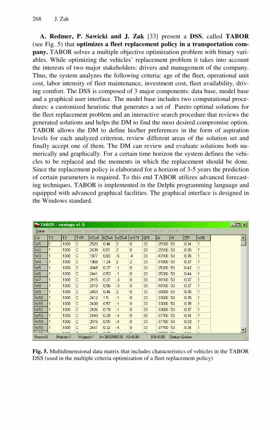
268 J. Zak
A. Redmer, P. Sawicki and J. Zak [33] present a DSS, called TABOR (see Fig. 5) that optimizes a fleet replacement policy in a transportation com-pany. TABOR solves a multiple objective optimization problem with binary vari-ables. While optimizing the vehicles’ replacement problem it takes into account the interests of two major stakeholders: drivers and management of the company. Thus, the system analyzes the following criteria: age of the fleet, operational unit cost, labor intensity of fleet maintenance, investment cost, fleet availability, driv-ing comfort. The DSS is composed of 3 major components: data base, model base and a graphical user interface. The model base includes two computational proce-dures: a customized heuristic that generates a set of Pareto optimal solutions for the fleet replacement problem and an interactive search procedure that reviews the generated solutions and helps the DM to find the most desired compromise option. TABOR allows the DM to define his/her preferences in the form of aspiration levels for each analyzed criterion, review different areas of the solution set and finally accept one of them. The DM can review and evaluate solutions both nu-merically and graphically. For a certain time horizon the system defines the vehi-cles to be replaced and the moments in which the replacement should be done. Since the replacement policy is elaborated for a horizon of 3-5 years the prediction of certain parameters is required. To this end TABOR utilizes advanced forecast-ing techniques. TABOR is implemented in the Delphi programming language and equipped with advanced graphical facilities. The graphical interface is designed in the Windows standard.
Fig. 5. Multidimensional data matrix that includes characteristics of vehicles in the TABOR DSS (used in the multiple criteria optimization of a fleet replacement policy)

Decision Support Systems in Transportation 269
Another DSS, developed by J.Zak et al, [68], [70], [71], [72], [73], [74] is a generic, prototype computer – system designed to assist the DM in managing both road and urban transportation systems. The framework of the DSS is based on the application of Multiple Criteria Decision Making methodology. Thus, the decision problems are formulated either as multiple criteria optimization or multiple criteria ranking problems. The road transportation section of the DSS provides the following functionality: fleet and crew sizing, vehicle routing and scheduling combined with crew scheduling, vehicle assignment to transportation jobs. The urban transportation section focuses on vehicle assignment and schedul-ing for the existing tram and bus network. The vehicle scheduling is combined with crew scheduling. The system is composed of an extensive two section data base (one for road and one for urban transportation), model base and a graphical user interface. The model base includes a collection of exact and heuristic algo-rithms that solve the above mentioned multiple objective decision problems. The vehicle assignment, routing and scheduling problems are solved by a hybrid evo-lutionary algorithm, while for crew scheduling the specialized heuristic procedure is applied. The fleet sizing problem is solved by exact combinatorial optimization algorithm. For all the problems a set of Pareto optimal solutions is generated and then evaluated by a multiple criteria interactive, search method. During searching for the compromise solution decision analysis phases alternate with computational phases. The DM can review solutions and analyze them both graphically and nu-merically. He/she can also generate another set of solutions. Based on the defined DM’s preferences the system searches for the most desired solution, which is as close as possible to the ideal or another selected reference point.
5.2 Urban Transportation DSS-s
Another category of transportation oriented DSS-s is focused on urban transporta-tion systems planning and management. Those systems deal with the following categories of decision problems: traffic control and management, vehicle routing and scheduling in urban areas combined with crew scheduling, designing inte-grated, multimodal passenger transportation systems, municipal solid waste col-lection and removal.
M. Dridi, K. Mesghouni and P. Borne [16] present a DSS for real – time, multimodal urban traffic control. The main objective of the DSS is to help the DM (regulator) in traffic regulation after the occurrence of disturbances. The main tasks of the DSS are as follows: to detect and analyze disturbances, solve the dis-turbances through finding feasible, and close to optimal schedules of selected vehicles on certain lines subject to specific disturbance – related constraints. In the proposed DSS the transportation network is modeled by Ordinary and Colored Petri Nets. The traffic network is characterized by a certain number of junctions and stops, and it is loaded by a set of vehicles. When the disturbance occurs the DSS “turns on” an automatic regulator that can choose several actions to palliate the disturbance. Those actions include: injection of an extra vehicle in the net-work, advance or delay of some vehicles, rerouting and rescheduling of vehicles on certain lines. Thus, the major task of the DSS is to reformulate the decision problem and find a feasible, semi – optimal solution for the new state of the urban

270 J. Zak
transportation system. Since the problem at stake is characterized by high compu-tational complexity metaheuristic procedures based on Evolutionary Algorithms are applied to solve it. An original, efficient genetic coding is applied to resolve the complex public transport scheduling problems. For the evaluation of generated solutions a multi - dimensional objective function is used. It includes the follow-ing criteria: waiting time, transit time and total travel time. The DSS is able to adjust the theoretical timetable to a newly encountered situation. The system has been developed for a transportation network in Valenciennes, France.
HASTUS [63] is a popular, commercial computer system for urban trans-portation planning. It is an integrated and modular DSS for transit scheduling, operations, and customer information. It has been implemented in 250 mass transit companies in 22 countries and used to schedule and manage bus, tram, subway, trolley, ferry, and commuter rail systems in cities with varied requirements, size, location and landform features, such as: New York, Sydney, Singapore, Barce-lona, Oslo or Vienna. An example of the vehicle schedule generated by HASTUS DSS is presented in figure 6. HASTUS also supports users in integrating multi-modal urban transportation systems, through synchronization of bus, rail and tram services (time tables) within certain metropolitan areas. Core modules of the HASTUS System include: Scheduling, Daily Operations, Customer Information, Analysis and Planning. Scheduling module assists in describing the route network and defining desired timetables. Vehicle and Crew Scheduling problems are solved by specialized heuristic algorithms and customized metaheuristic proce-dures. Based on the optimization process cost – saving vehicle and crew schedules as well as multi – day rosters are created. Daily Operations module allows DM-s to manage daily service changes, as well as vehicle and operator assignments. Actual versus planned schedules can be compared and operators’ performance can be monitored. Customer Information module provides planned or real – time in-formation for passengers about the current status of the time table. All changes in and deviations from the schedule are reported, which allows passengers to plan their trips. Customer information is displayed on the web site, stop posters, IVR systems, and electronic signs. Analysis and planning module provides network and timetabling modeling functions, including synchronization and fleet require-ments minimization. Run time and ridership data analysis contribute to improved fleet utilization and enhanced service better tailored to customer needs. HASTUS scheduling algorithms produce costs savings in the range of 2% to 5% over both competing systems and manual methods.
S. Peng and H. Fan [29] present a DSS that contributes to the design of an urban inter-modal public transit network. The proposed computer - system is a useful tool for transport planners in carrying out service planning, and routing and scheduling of vehicles for an inter-modal transit network. The DSS can be used to help in the design of an integrated transit system with relatively complex factors or adjust an existing system under specific objectives and constraints. The DSS assists the DM in evaluation of alternative operating strategies of the mass transit system and helps him/her to search for the optimal one. The DSS is also capable of examining the relationships between important decision variables of a transit service and transit system parameters. Identification of those relationships

Decision Support Systems in Transportation 271
Fig. 6. Vehicle schedules for a concrete railway station generated by HASTUS DSS
(e.g. operating headway and operating costs) supports the process of designing or redesigning the integrated mass transit system in the most efficient way. The DSS is focused on the analysis of rail services combined with express bus services and feeder bus services. The assumed network has a number of rail and express bus lines fed by feeder-bus services. The inter-modal public transit network has an irregular service area divided into small zones. Zonal passenger trips are grouped into Origin – Destination (OD) pairs. Each rail and express bus line is a high-speed trunk line serving higher and lower demand OD pairs, respectively. The role of feeder bus services is to provide access to and egress from the trunk service stops in each zone. A combination of heuristics and analytical derivation is ap-plied to solve the optimization problem. A step-by-step strategy is used to opti-mize the rail, express bus, and feeder bus services separately. However, different transit modes are still considered jointly to reflect their dependence on each other. In each stage of optimization, the services optimized in the previous ones are still kept in the loop and are optimized together with new services found. The DSS is composed of three modules, corresponding to rail service, express bus service and feeder bus service optimization, respectively. The optimization of rail and express bus services is focused on cost minimization, while the optimization of feeder bus services concentrates on accessibility to passengers and service coverage. The DSS has been applied for designing an integrated mass transit system for a service area with 10 zones. The optimization yielded 11 rail lines and 7 express bus lines operating with different headways ranging from 1,5 to 6 minutes.

272 J. Zak
G. Giaglis et al. [21] propose a mobile, real – time (on – line) vehicle routing computer system for urban distribution of goods. The proposed DSS has a generic, original and innovative architecture based on seamless mobile and wire-less connectivity between delivery vehicles and distribution facilities. The system allows for real – time and event – driven operational fleet management based on the on-line recognition of certain events which occurrence transforms the existing state of the system into a new one. As opposed to the majority of vehicle routing systems which have a centralized character and produce a daily plan of static ve-hicle routes before the beginning of their execution, the proposed solution uses advanced mobile and positioning technologies to detect unforeseen events and transmit information about them in the moment when they occur directly from the affected trucks through a mobile network to headquarters and other vehicles. Thanks to an efficient re-planning algorithm (based on specialized heuristics and metaheuristics), the DSS is equipped with, the designed vehicle routing plan can be adjusted and appropriate modifications can be implemented. Those modifica-tions are transmitted back to the fleet in a timely fashion to respond effectively to the new system state. The DSS is designed to carry out the following tasks: obser-vation of the system’s state; recommendation on the type of intervention (local plan adjustments vs. global re-planning), definition of the system objectives (op-timization criteria). The DSS is composed of three major sub – systems: the back-end system (decision making module and ERP connectivity facilitation module), the wireless communication sub-system (mobile access terrestrial network and positioning system) and a front end sub-system (user interface, local computations module, interaction module between on-board truck computer and the back-end system).
G. Tavares et al. [43] and P. Matis [27] present two different DSS-s that handle the street routing problem. The first one supports the user in solving a specific case of street or arc routing problem, which is the municipal solid waste collection. The proposed DSS concentrates on fuel savings through optimization of municipal solid waste transportation routes. The second DSS is a universal platform for solving different categories of street routing problem. The author, in addition to classical optimization criteria used in vehicle routing problems (total length of routes, total delivery time) introduces other qualitative measures, named as “visual attractiveness”. G. Traves et al. [43] use in their DSS a geographic in-formation system (GIS) for 3D (3 – Dimensional) waste collection routes model-ing and then optimize the routes according to the criterion of minimum fuel consumption. The GIS 3D routes modeling takes into account the effects of both the road inclination and the vehicle load. As opposed to the commonly applied approaches in which the shortest distance is searched for, the authors of the pro-posed DSS introduce the criterion of fuel consumption as the most important fac-tor that influences on waste collection costs. The solution procedure is composed of 3 phases, including: 3D modeling of the road network, calculation of fuel con-sumption factors for the entire 3D road network, performing the optimization of the municipal solid waste transportation for minimum fuel consumption. For the

Decision Support Systems in Transportation 273
calculation of the optimal routing the ArcGIS software, an extension of the ArcInfo and Network Analyst, is applied. The ArcGIS software utilizes advanced heuristic procedures for the optimization of the arc and street routing problems. The structure of the DSS proposed by P. Matis [27] includes 5 major components: GIS system, GIS Database, Heuristics, Integrator (Main user interface) and Inter-preter (Supporting visualization tool). P. Matis proposes in his DSS 9 alternative heuristic procedures for the optimization of the street routing problem, which can be classified as: Cluster – First, Route – Second Heuristics, Shaping Heuristics, Metaheuristics, Heuristics based on Visual Attractiveness, Hueristics with fuzzy clustering, Hueristics with a mixed model of node and arc service. All the above mentioned algorithms are available for use in the proposed DSS. The user speci-fies available time for calculation and desired parameters of results and the system chooses the best type of heuristics.
T. Randall, C. Churchill and B. Baetz [31] have developed a GIS (Geo-graphic Information System) based DSS for neighborhood traffic calming (NTC). The NTC is an extension of the Arc View GIS system focused on design-ing traffic calming / reduction programs (alternative scenarios to be implemented) for all street types, including arterials in the urban (residential) areas. The NTC DSS is a technologically advanced tool that generates suggestions on traffic calm-ing measures to reduce speed and volume and to prioritize safety and facilities for pedestrians, cyclists and transit. The concept of the DSS corresponds to the grow-ing public desire for safer streets. The DSS is dependent upon measured or per-ceived problems, road type and user objectives as well as current installation costs of traffic calming measures. It is constructed around a list of menu options that carry out the key tasks in evaluating the need for, and implementation of, neighborhood traffic calming. The NTC DSS is composed of three key menu options: 1) “Recognition and Display of Critical Areas for NTC”, 2) “Review and Selection of Traffic Calming Measures”, 3) “Placing the measures and evalu-ating their costs”. The first module identifies and displays graphically critical street segments that require NTC, based on three categories of factors: speeds exceed a desired threshold, daily traffic volume exceeds a desired threshold, spe-cial requests for traffic calming. The second module provides a wide variety of descriptive and visual information regarding the 29 available traffic calming measures / options for local, collector and arterial streets. Each measure is charac-terized; its intended benefits and drawbacks are presented. The third module is responsible for evaluation of the estimated costs of proposed combinations of NTC measures and their location (in a digitized form) on specific road segments identified on a map. Each output map is iterative, allowing a user to add and re-move traffic calming measures and reevaluate the cost of the plan. In the decision process on locating measures the DM is able to consider the following priority options: calm school, playground and pedestrian zones, make allowances for bikes on major collectors and arterials, prioritize access for transit on arterials. The functionality of the DSS is demonstrated based on its application to suburban Hamilton (Canada).

274 J. Zak
5.3 Airborne Transportation DSS-s
Since air transportation industry is very sensitive to any kind of wrong and / or imperfect decisions a lot of emphasis has been put on comprehensive and efficient decision making procedures in this branch. In addition, air transportation is a very capital – and cost - intensive industry; thus, it requires advanced algorithms that assure rational investments, adequate transportation assets utilization and appro-priate control over the level of day-to-day spending (running costs). Since the costs of air transportation, both for passengers and cargo, are much higher than in other transportation modes, the level of service offered must be very satisfactory. As a result air transportation industry has developed many computer–based DSS-s that provide transportation solutions focused on: safety and reliability assurance, customer satisfaction and cost rationalization. The most popular DSS-s for air trans-portation are described below.
AeroTURN [63] is a CAD-based computer system for creating airside de-signs, evaluating aircraft ground maneuvers, and meeting clearance and space requirements. The AeroTURN DSS makes it possible to place multiple aircraft lead-in lines, set jet blast envelopes, mark aircraft nosewheel path, run airside animations, and perform other operations. The AeroTURN DSS is created for airport planners, designers and engineers. The CAD platform is combined with the simulation package, which both facilitate gate and aircraft stands design supple-mented by aircraft maneuvering simulation and ground support vehicle movement at airport facilities. The designers are equipped with a full library of technical airport equipment, such as: boarding bridges, aircraft staircases, and a complete collection of aircrafts.
Another air transportation DSS is Sabre AirFlite Schedule Manager (SAFSM), that belongs to a wider family of Sabre Air Solutions [63]. SAFSM is a universal flight scheduling computer system that can be customized to specific needs of each airline. It enables an airline to develop semi – optimal flight sched-ules and/or continuously adjust them to fluctuating demand and changing cus-tomer needs. The proposed DSS has an interactive character and allows the user (scheduler) to generate a large number of solutions (flight schedules), review them and explore better options (see Fig. 7). During the optimization process the DM is supported by graphical and numerical tools that enable him/her to view, edit and report flight schedule information. The scheduler is also advised by the system how to make certain changes and adjustments in the proposed schedule. Since different options of flight schedules with their corresponding values of the objec-tive functions are presented to the DM, he/she gets deeply involved in the optimi-zation process and becomes more and more experienced in finding an optimal solution. The system helps the DM to educate himself/herself while leaving him/her the responsibility to control the decision – making process. In addition, SAFSM also supports the creation of a corporate-wide flight-scheduling database and provides easy connectivity to legacy systems. The system can be utilized in combination with other Sabre products such as: Codeshare Manager, Profit Manager and Fleet Manager.

Decision Support Systems in Transportation 275
Fig. 7. The Gantt chart for aircraft transportation tasks generated by Sabre AirFlite Sched-ule Manager
Codeshare Manager offers different airlines a way to develop codeshare flight schedules when they agreed to cooperate and codeshare their flights. Using the operational flight schedules for two airlines, the computer system builds connec-tions to identify potential codeshare flights and eliminate useless repetitions of certain connections. Eventually, Codeshare Manger adjusts flight schedules of both airlines and assigns flight numbers based on flight number assignment rules. Both SAFSM and Codeshare Manager allow the airlines to considerably reduce schedule development time. Profit Manager evaluates the profitability of a given schedule to assist in strategic, long-range planning. It can identify strengths and/or weaknesses within a carrier’s schedule as well as quantify the impact a particular schedule may have on revenues and costs. Profit Manager forecasts the typical-week profitability for a complete O&D network. On average it generates 1% to 3% annual incremental revenue. Fleet Manager enables an airline to optimally allocate fleet capacity to further improve the profitability of a schedule. It employs global optimization techniques to provide an airline with strategic and tactical analysis support when developing profitable and operationally feasible schedules. In the optimization process a patented O&D passenger flow model is applied. Fleet Manager enables schedulers to swap aircraft assignments, re-time and cancel flights, improve utilization and minimize aircraft towing. It can increase annual profits by 0.5% to 3%.

276 J. Zak
In addition, Sabre offers a range of traditional computerized air transportation products, such as: advanced on-line flight reservation (SabreSonicRes) and pas-sengers booking (SabreSonicWeb) systems combined with electronic ticketing (SabreSonicTicket).
Another example of air transportation DSS is a computer – based product de-veloped by A. Cheung, W. Ip and D. Lu [12]. The authors propose a generic DSS for aircraft maintenance services industry that supports the DM in a complex personnel planning problem. The major task of the proposed DSS is to allocate labor resources to specific maintenance activities required to check and enhance the technical condition of the aircraft. The system also helps the user to select the best candidates for concrete tasks under the shortage of experienced and qualified engineers. In the evaluation of candidates and allocation of manpower several criteria / variables (including intangible ones) and constraints (aviation authorities regulation, safety laws, qualifications of the employees, cus-tomers’ requirements) are taken into account. The authors utilize in the proposed DSS fuzzy analytical hierarchy process (AHP) approach for weighting the impor-tance of several intangible criteria and rank the candidates from the best to the worst. A two-stage computational procedure is applied to rank candidates for a specific maintenance job. In the first one a larger number (e.g. 40) of employees/ engineers is considered and evaluated by a set of critical criteria (Aircraft Mainte-nance Engineer License, Airplane and Airlines Approval, Experience, including Airplane and Airlines experience, and Specialization). In the second stage a lim-ited number of candidates (e.g. 5–10) that have been highly ranked in the first phase are further considered. They are evaluated by a set of such parameters as: training, regulations, shift time and human factor. In the second phase of the selec-tion process the shift schedule of the chosen employee is matched with the flight schedule. As proven by the number of experiments, the proposed fuzzy – AHP based DSS provides better human resource management and higher productivity for the aircraft industry than other applied methods.
I. Manataki and K. Zografos [26] propose a generic DSS for airport termi-nal planning and performance analysis. The system is based on the mesoscopic simulation model of the airport terminal operations and systems dynamics ap-proach that takes into account numerous interactions between certain components of the airport terminal as well as phenomena and processes that take place in it and influence on each other. The authors claim that the proposed system fills the gap between too detailed (microscopic) models that refer to specific airport terminals and too aggregate (macroscopic) models that do not reflect terminal operations with sufficient detail. The proposed DSS has a modular and hierarchical architec-ture, and an interface enabling quick and user friendly model building. The system provides capabilities of being adaptable to the configuration and operational char-acteristics of a wide spectrum of airport terminals. The proposed DSS takes into account three major factors/ dimensions that affect the overall complexity of the analyzed airport terminal, i.e.: topological dimensions, operational dimensions and performance dimensions. The following three methodological assumptions created the framework for the development of a generic, yet flexible model for the analy-sis and evaluation of terminal performance: 1) model capability to cope with

Decision Support Systems in Transportation 277
complexity of the airport terminal system; 2) model capability to analyze and model airport terminal operations in a holistic perspective; 3) model flexibility, so that it can be easily adaptable to the airport under consideration. The overall ar-chitecture of the DSS is structured into two hierarchical levels: 1) decomposition of the airport terminal system into a set of Airport Functional Areas (AFAs), 2) decomposition of each AFA into Service Facilities (SF modules). This architec-ture corresponds to the terminal simulation metamodel. This metamodel includes: “Customer Type” that is associated with a respective “Service Process”, supported by “Facilities”, “Resources” and “Service Providers”. The airport terminal model is based on the object – oriented simulation and requires the following input data: 1) Demand characteristics; 2) Airport terminal physical configuration; 3) Cus-tomer groups’ characteristics; 4) Operational / Service characteristics. The DSS is equipped with both numerical and graphical capabilities. The application of the systems allows the DM to carry out multiple dimension analysis, including: pas-senger arrival pattern to the airport by mode of transport, queue lengths and wait-ing times at different service areas (e.g. passport control, check – in counter) dur-ing different time periods, peak and off - peak hours behavior of different facilities (e.g. belt conveyers). Major features and capabilities of the proposed DSS have been demonstrated through the analysis of the International Airport terminal in Athens (Greece).
Another air – transportation DSS is a commercial, computer - based product called Global Logistics Network (GLN) [63], a successor of the Global Freight Exchange (GF-X) System. GLN is an advanced end-to-end shipment manage-ment computer system for the air cargo industry. The system is characterized by the following functionality: 1) Manages electronically the entire air shipment lifecycle, including bookings, air waybills, house waybills, status massages, and customs procedures; 2) Manages rates from the initial booking all the way through to invoice presentation, bill of loading rating and audit; 3) Helps the users to com-ply with customs regulations and leading industry standards. Its major features are as follows: Centralized Rates and Reservations (CRR), Automated and Elec-tronic Air Way and House Way Bills (AEAHWB), Client Configured Data Cap-ture (CCDC), Supply Chain Visibility and Status Massages (SCVSM), Customs Filings and Compliance (CFC), Importing and Exporting Data (IED), Trading Partner Connectivity (TPC), Planning and Optimization (PO), Order Execution (OE) and Settlement (S). Many of these functions correspond to the sequential operations of the order fulfillment process. The CRR module provides on a regular basis, on – line information about service rates, contracts and shipment details. Carriers submit the following information about their services to this module: available fleet and its capacity, possible routing, characteristics of core and sup-plementary services, service rates. Forwarders can access carriers’ information through CRR module and make electronic booking. Once the reservations are made the AEAHWB module electronically creates an Air Waybill and House Waybill that are sent to the airlines and to the shipper, respectively. When the delivery process starts communication of status messages and ongoing updates are distributed, which allows both service providers and customers to monitor all the stages of the order fulfillment process in the whole supply chain. The GLN DSS

278 J. Zak
provides a single access point to customs electronic initiatives from various gov-ernments around the world. IED and CCDC functions allow the manipulation on data off-line and its import in different formats, as well as the transfer of the data to the users’ back – office legacy systems in the appropriate standard. The TPC function facilitates the trade contacts between suppliers and customers and allows forwarders and carriers to reduce customer acquisition costs. The PO function allows operators to select carriers based on different measures (cost, service level, commitment to customers). Thanks to the OE function loads are electronically tendered to carriers, where they can automatically accept and respond to a pickup, provide tracking as required, and show prove of delivery. The S function supports the electronic delivery of invoices from carriers and stores all contracts and tariffs for future reference. The GLN DSS has been successfully used by several airlines, including American Airlines Cargo.
Another example of an air transportation DSS is an intelligent computer sys-tem developed by W. Cheung, L. Leung and P. Tam [13], focused on service network planning. A proposed PC – based, prototype Intelligent Decision Support System (IDSS) integrates DSS with an Expert System (ES), to provide guidance to the DM during the network planning process. A two-stage methodology, making use of both macro – planning optimization model and operational planning simu-lation model, has been applied and implemented in the proposed IDSS. The macro – planning model is formulated as a mixed integer programming problem. It aims at searching (in a 10-year horizon) for the distribution network configuration (lo-cations of facilities, definition of their capacities and years of installations, assignment of shipment routes) with minimal cost settings subject to aggregate customer demands, facility capacity and service response time. A simulation model is used to validate and evaluate the performance of the given distribution network at the operational level. It takes into account operational fluctuations in the distribution system and random behaviors of its components. A simulation software ARENA have been used to model and simulate the air express courier’s daily operations. The distribution system has been evaluated based on two per-formance measures: service coverage and service reliability. While using the two-stage methodology, the DM needs to be familiar with both models because he/ she manipulates them iteratively using his/her expert knowledge in a domain to reach a planning solution. The authors integrate the original DSS with an ES in such a way that ES is an add-on to the DSS. The structure of the IDSS includes: model base with optimization model and simulation model, model and data base man-agement systems (MBMS and DBMS), knowledge base, interface engine and user’s interface. The proposed IDSS has been applied in the design of a service network for a major air-express courier DHL with 33 demand zones. In the test experiments the following operational targets have been defined: facility utiliza-tion less than 85%; service cut-off time not earlier than 5:15 p.m.; service cover-age of at least 90% and service reliability of at least 95%. The interaction between the simulation and optimization model have been demonstrated. The IDSS pro-vided intelligent guidance to the planner on the overall planning flow logic, advis-ing on necessary modifications and suggesting which model should be re-run. At the micro – level the IDSS identifies the causes of the problems and advices the

Decision Support Systems in Transportation 279
DM on certain actions that should be undertaken to change the inconvenient situa-tion. One of the drawbacks of the proposed IDSS is the fact that it can not play the role of the modeler. Computational tests have proven that manipulation of data is tedious and often prone to errors. The DM-s need extensive training to properly use the models.
R. Freling, R. Lentink and A. Wagelmans [20] have developed a DSS for crew planning in passenger both air and railway transportation, called Har-mony CDR (Crew Duty Rostering). The system is based on the exact and heuris-tic branch-and-bound and branch-and-price algorithms and designed to generate optimal crew schedules and crew rosters. Two different approaches to crew scheduling and rostering are implemented in the proposed DSS. In the first one optimal crew schedules are generated before optimal crew rosters, while in the second approach two planning problems are solved in an integrated manner. The decision problem is formulated as a set partitioning problem with binary and con-tinuous variables and a minimized cost objective function, subject to classical constraints (labor code regulations, agreements). The solution algorithm of the decision problem is based on LP relaxation and column generation procedure. The Harmony CDR system supports the entire planning process, which is divided into long and short term planning (rostering and operations control), realization and evaluation. It helps management to determine: the capacity needed to perform the tasks, the permanent and temporary staffing levels needed to meet the required capacity, allowed vacations, standbys required, etc. for the given period. The pro-posed DSS is capable of generating several alternative solutions - crew schedules and crew rosters (in a relatively short time) that satisfy both economic (manage-ment) and social (employees) interests. Three categories of conflicting criteria are taken into account: efficiency – cost minimization with respect to the number of uncovered tasks and the number of required duties or crew; welfare – the work-load of the rosters should be equally spread among the crew; robustness – duties or rosters should be robust with respect to delays (e.g. by imposing a maximum number of vehicle changes). The system recognizes different categories of crew classes in airline and railway industry, such as: cockpit and cabin crews in airplanes and train drivers, ticket controllers and guards in trains, that carry out different crew functions. The framework of the DSS is implemented in the C++ programming language, making full use of its object oriented nature. The system is composed of the following modules: Input and Output Translators, Linear Pro-gramming (LP) and Integer Programming (IP) Solvers, Network Algorithms Module, Column Generator, Rules Checker and Optimization Coordinator. The Harmony CDR DSS has been successfully implemented in several companies, including: a charter airline, a European regional airline, the Dutch Railway and RailRest (catering company of the high speed train in Western Europe). The ana-lyzed instances included between 500 and 2200 duties (tasks) and 55 to 126 crews.
5.4 Railway and Seaborne Transportation DSS-s
Railway and seaborne transportation are the areas where advanced computer systems are less popular and where their application is not so frequent. Despite this fact several applications of DSS in railway and seaborne transportation are

280 J. Zak
presented below. We hope that results generated in other transportation industries will encourage in the future railway and seaborne companies to make a better use of existing computer - based solutions.
N. Bojovič [6] proposes a prototype DSS for rail freight car fleet sizing and scheduling problem. The system utilizes a dynamic network optimization model with a time dependent demand, assigned to the edges of the network. The DSS optimizes the number of rail cars for the analyzed railway system in which full – truck - loads transportation is carried out only. The system decides on the number of loaded and empty movements of the cars between certain nodes of the network in different time periods. As a result it determines the required number of rail cars in the fleet, based on the optimization of the cost function, that includes: transportation (movement) costs (of loaded and empty vehicles), fleet waiting costs, fleet maintenance costs and penalty costs (for unfulfilled orders). The DSS generates different optimal numbers of vehicles that satisfy the demand in certain time periods.
Another example of the railway transportation DSS is the prototype computer system developed by H. Sheralie and C. Tuncbilek [39]. The system provides the DM the ability to define an optimal fleet management strategy that results in determining the optimal number of rail cars for a certain railway system. Two strategic, time – space decision models of static and dynamic character are imple-mented in the system. The first one is formulated as a transportation problem, with a homogenous fleet. In this case, given the daily demand for transportation ser-vices, distances and riding times between origins and destinations the number of empty return movements is optimized. The fleet size is determined by the quotient of the total riding time during a day and the expected daily number of rides (loaded and empty) per each vehicle. In the second model, being an extension of the first one, a spatial (time – distance) network have been introduced into a tradi-tional transportation problem. This network allowed presenting the empty move-ments of vehicles between origins and destinations in specific time periods. Again, the number of empty movements has been optimized. To this end a heuristic de-composition algorithm has been applied. Finally, the fleet size has been deter-mined in the same way as in the first model. The proposed DSS allows the DM to customize one of the above described models to a specific decision situation and generate the optimal number of rail cars for the whole analyzed railway system.
There are several commercial software packages for railway – transporta-tion, including: InfraManager [63] and Ramsys [63]. InfraManager is a com-puter – based planning and decision support tool designed and developed for Italian Railways (RFI). It helps the DM-s to design, maintain, control and develop the railway transportation system. InfraManager supports managerial activities and decision making processes focused on: demand analysis for railway transpor-tation services, fleet and transportation infrastructure management, human re-source management, safety control and customer service. InfraManager assists the user in designing and redesigning of the transportation network, suggests network extensions and reductions, schedules trains and crews, analyzes technical condi-tion of vehicles and railroads, recommends check-ups and maintenance services. The application of InfraManager in Italian Railways resulted in certain cost

Decision Support Systems in Transportation 281
reductions, introduction of innovative solutions and substantial improvement of customer service. Ramsys (Railway Asset Management System) is an advanced, generic and modular DSS designed to support data analysis for optimized planning of the railroad infrastructure maintenance and renewal (see Fig 8).
Fig. 8. Graphical diagnostics and technical condition analysis of the railway transportation infrastructure in Ramsys DSS
Ramsys is a combined hardware and software tool that collects and processes a wide range of data relevant to the technical condition analysis of the railroad in-frastructure. The system measures a number of diagnostic parameters, detects technical problems in the railroad network and evaluates its technical condition. It bridges diagnostics and maintenance engineering for railroad infrastructure through a process oriented activities that include: monitoring of the infrastructure and resulting in the generation of measurement records, analyzing the situation and detecting defects, planning interventions and issuing alerts, scheduling main-tenance activities and creating work orders, controlling the execution of mainte-nance activities. The railroad system is visualized in Ramsys and particular segments of the network where technical problems are detected are displayed on the screen. The graphical charts with the diagnostic signals and parameters help the DM-s (planners) to analyze the existing situation and develop a set of interven-tion scenarios. Adopting advanced multilevel segmentation Ramsys can

282 J. Zak
effectively process and perform reasoning based on any type of data (local meas-uring point, segment, track section, line, maintenance department, maintenance contractor’s area, region, etc.) to provide local and global knowledge of the rail-way infrastructure both in terms of the network condition (past, current and future) and maintenance and renewal requirements. Ramsys, which is equipped with a collection of optimization tools, optimizes the costs of the maintenance and re-newal plan subject to traffic and budget constraints. Based on that optimization the computer system schedules maintenance activities and issues work orders. Addi-tional examples of the railway transportation DSS-s are the systems described above: Harmony CDR for crew scheduling and rostering [20] and Hastus [63] that can be applied for planning light train operations, especially in the metropoli-tan areas.
As far as seaborne transportation is concerned the most emphasis is put on the development of DSS-s solving the ship routing and scheduling problems. However, most of ocean shipping companies do the planning of fleet schedules manually based on their experience. Only a few use optimization – based DSS-s. Since different categories of seaborne operations, including: industrial shipping, commercial cargo shipping, tramp and liner shipping and naval operations, require different approaches to vessels routing and scheduling, thus, the developed DSS-s have a customized character and can be applied in very specific situations. On the other hand the similarities between various categories of ship routing and schedul-ing problems result in applying similar techniques for solving those problems. In the majority of cases the most commonly used algorithms include: linear pro-gramming (LP) with heuristics, integer and mixed integer programming, set parti-tioning and simulation.
D. Bausch, G. Brown and D. Ronen [4] present a DSS for medium – term (2–3 weeks) scheduling of a fleet of coastal tankers and barges transporting liquid bulk products among plants, distribution centers, and industrial customers. The ships may have up to 7 fixed compartments, which translates into several categories of products to be transported by the same vessel. In addition to the specified set of loads that must be shipped, there may be some optional back hauls available. These back hauls generate income and may be taken if they are profit-able. The vessels scheduling problem is formulated as an elastic set partitioning problem, in which some constraints may be violated at a cost. The solution method exploits the problem knowledge in an elastic enumeration procedure. The decision problem is solved by generating all feasible schedules because it is rela-tively well constrained. The DSS is equipped in a user – friendly interface based on a simple Excel spreadsheet. This solution makes the system usable via a variety of natural languages. The dispatchers all over the world can communicate via the spreadsheet independent of their mother tongues and view recommended sched-ules displayed in Gantt charts.
K. Fagerholt [19] has developed a similar DSS for vessel fleet scheduling, called TurboRouter. While designing the system the author defined the following principal prerequisites for the vessel fleet scheduling DSS: 1) It should guarantee

Decision Support Systems in Transportation 283
a quick response time, i.e. the solutions should be generated in a short time; 2) The solutions must be featured by high quality (near optimal solutions); 3) The DSS must be flexible in modeling real-life constraints; 4) It should allow a good inter-action with the user. To satisfy those assumptions an optimization routine consist-ing of two different heuristic algorithms has been developed. The first one is the insertion algorithm that processes the cargo sequentially, inserting one at a time into the work schedule until all cargos are processed. The second algorithm is a hybrid local search that improves any generated solution. The optimization routine implemented in the proposed DSS accommodates the following features: opti-mizes with respect to financial results and fleet capacity utilization in a user-specified planning period, takes into account cargo time windows and vessel ca-pacities, checks compatibility between vessel and loading /discharging ports as well as vessel equipment and product characteristics, takes into account multiple products, parcel cargos and full shiploads as well as split cargos, combines spot and contract cargos, includes or excludes time charter vessels. The interface of the DSS has a spreadsheet – like form representing the assignment of cargos to the vessels. Specific colors used in the spreadsheet represent physical constraints, timing constraints and assignments of cargos to vessels. In addition, the visualiza-tion of generated schedules is possible. The DM can view Gantt diagrams, capac-ity utilization charts, geographic location of the vessel routes in the sea charts.
5.5 Transportation – Oriented DSS-s Applied in Different Industries and Multimodal DSS-s
Since the natural feature of transportation is the transfer of different categories of goods and physical integration of different links/ organizations/ industries of the supply chain certain transportation solutions refer to specific industries they are designed for. Thus, selected DSS-s are focused on solving transportation decision problems in certain branches. The below described DSS-s involve the following special cases of transportation decision problems encountered in different indus-tries and countries: motor carrier selection for high – pressure gas containment equipment manufacturer in USA, routing and scheduling of logging trucks in forest industry in Sweden, designing dispatching routes for a meat manufacturer in Spain. Also two examples of multimodal transportation DSS-s are presented.
C.-C. Kuo and F. Soflarsky [24] present a DSS focused on motor carrier se-lection for a manufacturing company producing high – pressure gas contain-ment equipment in the United States. The computer system assists the traffic manager of the manufacturing company in the decision making process focused on selecting the most suitable trucking companies for delivering finished goods to selected customers. The selection of the carrier is combined with scheduling of transportation services. The considered DSS takes into account full – truckload (FTL) carriers and less- than – truckload (LTL) carriers and assumes three alterna-tive shipping fees: flat rate per shipment, variable rate per mile (kilometer) with minimum charge and variable rate per pound (kilogram) of the load with mini-mum charge. The major concern in the carrier selection process carried out by the DSS is cost minimization. Thus, the DSS ranks the carriers from the cheapest to

284 J. Zak
the most expensive for a particular shipment and selects the best variant. In addi-tion, the system optimizes the shipping plan through consolidation of orders being shipped into the same geographical area in a similar time range. Based on a rela-tively simple linear – programming model the DSS defines an optimal shipment plan. This automatically generated plan is compared with the manual, intuitive plan proposed by a traffic manager. The study shows that in some instances (sev-eral shipments) the manual, intuitive procedure outperforms the automated method. It reveals, however, that the overall transportation expenditures can be reduced by 3%.
G. Andersson et. al. [2] characterize RUTTOPT – an advanced, computerized DSS for routing and scheduling of logging trucks in the forest industry in Sweden. The system is composed of several modules, including: the main applica-tion (Central Module), which is the central user interface of the RUTTOPT DSS. This user interface is composed of 3 major components, such as: Internal Database, Geographic Information System (GIS) and Presentation Component. It offers dif-ferent functionality for: viewing geographical data extracted from GIS, editing data, developing reports and analyzing generated results. All information and results can be viewed on maps, Gantt schedules and in tables, thus they all have both numeri-cal and graphical form. The Internal Database contains all relevant information required to formulate and solve the vehicle routing problem, such as: supply and demand information, trucks characteristics, information about depots and required changes of drivers, definition of time windows, etc. It is linked with the external Swedish National Road Database (NVDB) that contains digital information of all Swedish roads. Those roads of approximately 500 000 kilometers are described geometrically and topologically with additional information on each road segment. NVDB constitutes 2nd Module of the RUTTOPT DSS. This module also includes a tool to compute distances between locations. The 3rd Module – Route Planner is an optimization package that finds optimal routes and schedules for all trucks. This module utilizes a two-phase algorithm based on linear programming (phase 1) and an extended version of unified tabu search algorithm (UTSA), proposed by Cor-deau et al. In the first phase feasible flows between supply and demands points are defined and optimal transport nodes (pick-up and delivery points) are generated through the application of linear programming. In the second phase the vehicle routing problem is solved with the application of UTSA. The RUTTOPT DSS has been applied in several instances ranging from 10 to 110 trucks with a planning horizon of 1 to 5 days. The DSS proved to be useful in relatively large instances of the VRP. The computational results generated by the RUTTOPT system assured potential savings of 5% to 30%.
Another example of transportation – oriented DSS, serving in a different branch is RUTAREP, developed by J. Belenguer, E. Benavent and M. Marti-nez [5]. The system helps the DM to design dispatching routes for a medium-sized meat company in Spain. The problem solved by the DSS is an extended variant of the vehicle routing problem with the following specific characteristics: a hetero-geneous fleet of vehicles, soft time windows, a multiple objective cost function

Decision Support Systems in Transportation 285
including total delay (lateness) of deliveries and total distance traveled, a partition of orders by zones and vehicles (with additional constraint that each vehicle must service a predefined percentage of orders). The problem is solved by a set/ combi-nation of specialized heuristics and metaheuristics, that take advantage of specific features of the decision problem the meat company faces. The semi - optimal solution is generated by a two-phase computational procedure. In the first phase a constructive heuristic procedure based on the M. Solomon insertion algorithm is used to design a feasible route for each vehicle. This route includes as much or-ders of its zone as possible. All unrouted orders are inserted into other routes, regardless its zone by additional heuristic. Once a feasible solution is obtained an improvement algorithm based on Tabu Search and inspired by the work of E. Tailard et al. is applied. The system allows to minimize the total distance traveled by vehicles and the total delay (lateness) incurred when serving the orders as well as to balance both objectives. The system has been coded in Visual C++ and runs on a personal computer under Windows system. It is characterized by the follow-ing features/ functionalities: reading, editing and handling of the data regarding customers, vehicles and orders (including geographical data in the digital form); building, displaying and modifying the routes; computing distances and travel times between customers; optimizing the dispatching routes. RUTAREP DSS substantially improves the existing solutions by 9% - 15% and by 81% - 88% in terms of total distance and total delay (lateness), respectively.
Two examples of multimodal transportation DSS-s include the proposals of: B. Vannieuwenhuyse, L. Gelders and L. Pintelon [50] and W. Dullaert et al. [17]. The first product, called Promodi is an online DSS for transportation mode choice. It collects through the Internet data from practitioners about their perception on different modes of transportation, processes the data and transforms them to the importance of selected criteria that evaluate the modes for the logistic chain and to the performance of particular modes on specific criteria. The system takes into account the following criteria while evaluating the transportation modes: transportation cost, reliability, flexibility, transportation time, safety, ca-pacity, density of network, regulation and legislation, impact, image, strategic elements. Promodi utilizes the multiple criteria consensus method to evaluate the variants. Based on that evaluation the ranking of transportation modes is generated and displayed both numerically and graphically. The second DSS, called Mam-MoeT is a real time communication platform in which intelligent software agents handle communicative tasks, exchange desired amounts of information among different users. The software agents, i.e. pieces of software represent a single user. They take over various communicative tasks in real – time and allow exchange of information between partners in the supply chain (shippers, forwarders, transport-ers, customers). The DSS also allows for high level of customization, so that users can decide themselves on how much information to share (trust issue). MamMoeT produces and uses common exchange protocols which act as translators between different systems.
Table 1 presents a comparison of selected transportation – oriented DSS-s.

286 J. Zak
Tra
nspo
rtat
ion
orie
nted
DSS
M
odal
fo
cus
Und
erla
ying
de
cisi
on m
akin
g m
etho
dolo
gy
App
licat
ion
area
; sub
-je
ct s
cope
&fo
cus
Prod
ucer
R
epor
ted
bene
fits
Tra
nsC
AD
ro
ad, u
rban
, ra
il,
pipe
line
optim
izat
ion
flee
t man
agem
ent,
tran
spor
tatio
n ne
twor
k an
alys
is
Cal
iper
C
orpo
ratio
n - c
ost s
avin
gs
- sub
stan
tial r
educ
tion
of m
a-
- inc
reas
ed u
tiliz
atio
n of
the
- hig
her l
evel
of c
usto
mer
- bet
ter c
ontr
ol o
f the
tran
spor
-
L
ogix
Cen
tral
Sys
tem
ro
ad
optim
izat
ion
flee
t man
agem
ent
(veh
icle
rout
ing
and
sche
dulin
g)
DPS
In
tern
atio
nal
- red
uctio
n of
tota
l dis
trib
utio
n
- sub
stan
tial r
educ
tion
of m
a-
- inc
reas
ed u
tiliz
atio
n of
the
- hig
her l
evel
of c
usto
mer
- bet
ter c
ontr
ol o
f the
tran
spor
-
R
oute
Pla
nner
ro
ad
optim
izat
ion
flee
t man
agem
ent
(veh
icle
rout
ing
and
sche
dulin
g)
The
Des
cart
es
Syst
ems
Gro
up
Inc.
- 10-
30%
redu
ctio
n in
fuel
co
sts,
- 2
0%-4
0% im
prov
emen
t in
nua
l pla
nnin
g,
fle
et,
ser
vice
,
tat
ion
proc
ess,
cos
ts u
p to
25%
,
nua
l pla
nnin
g,
fle
et,
ser
vice
,
tat
ion
proc
ess,
Tab
le 1
. Bas
ic f
eatu
res/
char
acte
rist
ics
of s
elec
ted
tran
spor
tati
on o
rien
ted
DS
S-s

Decision Support Systems in Transportation 287
- 10%
-25%
incr
ease
in th
e
- up
to 5
0% re
duct
ion
in la
bor
Tr
ucks
tops
ro
ad
optim
izat
ion
fleet
man
agem
ent
(veh
icle
rout
ing
and
sche
dulin
g)
Map
Mec
hani
cs
10-
30%
redu
ctio
n in
fuel
cos
ts,
- 20%
-40%
impr
ovem
ent i
n
- 10%
-20%
incr
ease
in th
e
- up
to 5
0% re
duct
ion
in la
bor
X
enio
s ro
ad
optim
izat
ion
fleet
man
agem
ent
(veh
icle
rout
ing
and
sche
dulin
g); e
vent
m
anag
emen
t
Aris
totle
U
nive
rsity
of
Thes
salo
niki
, A
then
s U
nive
rsity
of
Econ
omic
s an
d B
usin
ess
- cos
t sav
ings
- r
educ
tion
of m
anua
l pla
nnin
g
TAB
OR
ro
ad
optim
izat
ion
fleet
man
agem
ent
(veh
icle
repl
acem
ent)
Pozn
an
Uni
vers
ity o
f Te
chno
logy
- sub
stan
tial r
educ
tion
of th
e
-10-
20%
redu
ctio
n of
the
ve-
- red
uctio
n of
flee
t rep
airs
and
se
rnic
e ta
sks
veh
icle
util
izat
ion,
cus
tom
er s
ervi
ce le
vel,
int
ensi
ty o
f the
pla
nnin
g p
roce
ss.
veh
icle
util
izat
ion,
cus
tom
er s
ervi
ce le
vel,
int
ensi
ty o
f the
pla
nnin
g p
roce
ss.
fle
et a
ge,
hic
le- k
ilom
eter
cos
t,

288 J. Zak
- 15-
20%
incr
ease
of f
leet
H
AST
US
mul
timod
al
urba
n op
timiz
atio
n,
urba
n tr
ansp
orta
tion
plan
ning
(tra
nsit
sche
-du
ling,
ope
ratio
ns, a
nd
cust
omer
info
rmat
ion)
GIR
O In
c.
- cos
t sav
ings
of 2
%-5
%
- sub
stan
tial r
educ
tion
of m
a-
Aer
oTU
RN
ai
rbor
ne
sim
ulat
ion
ai
rsid
e de
sign
ing
Tra
nsof
t So
lutio
ns In
c.
- cos
t sav
ings
- s
ubst
antia
l red
uctio
n of
ma-
Sa
bre
Air
Flite
Sch
e-du
le M
anag
er
airb
orne
op
timiz
atio
n,
flee
t man
agem
ent
(flig
ht s
ched
ulin
g)
Sabr
e A
irlin
e So
lutio
ns
- p
rofi
tabi
lity,
- e
nhan
ced
stra
tegi
c pl
anni
ng,
- im
prov
ed s
hort
-ter
m p
lan-
- im
prov
ed a
ircr
aft u
tiliz
atio
n - e
nhan
ced
holid
ay a
nd s
peci
al
- cos
t sav
ings
Glo
bal L
ogis
tics
Net
wor
k ai
rbor
ne
optim
izat
ion,
sh
ipm
ent m
anag
emen
t, fl
eet m
anag
emen
t T
he D
esca
rtes
Sy
stem
s G
roup
In
c.
- cos
t sav
ings
- s
ubst
antia
l red
uctio
n of
ma-
H
arm
ony
CD
R
airb
orne
, rai
lop
timiz
atio
n pe
rson
nel m
anag
emen
t (c
rew
sch
edul
ing
and
rost
erin
g),
OR
TE
C b
v - c
ost s
avin
gs
- sub
stan
tial r
educ
tion
of m
a-nu
al p
lann
ing,
in
crea
sed
ava
ilabi
lity
and
driv
ing
com
- f
ort
nua
l pla
nnin
g,
nua
l pla
nnin
g,
nin
g,
eve
nts
sche
dulin
g,
nua
l pla
nnin
g,

Decision Support Systems in Transportation 289
Ra
msy
s ra
il op
timiz
atio
n,
data
min
ing
in
frastr
uctu
re m
aint
en-
ance
and
rene
wal
M
ERM
EC
Gro
up
- im
prov
ed tr
affic
safe
ty &
- enh
ance
d ne
twor
k av
aila
bilit
y
- dec
reas
ed m
aint
enan
ce c
osts
&
ass
et li
fecy
cle,
Turb
oRou
ter
wat
erbo
rne
optim
izat
ion
fleet
man
agem
ent
(flee
t sch
edul
ing)
M
ARI
NTE
K
Solu
tions
- c
ost s
avin
gs
- sub
stant
ial r
educ
tion
of m
a-nu
al p
lann
ing,
Ru
ttOpt
ro
ad
optim
izat
ion
fleet
man
agem
ent
(veh
icle
rout
ing
and
sche
dulin
g)
Skog
fors
k - c
ost s
avin
gs o
f 5%
-30%
.
Prom
odi
mul
timod
al
MCD
M
Tran
spor
t Man
agem
ent
(mod
al c
hoic
e)
Kat
holie
ke
Uni
vers
iteit
Leuv
en
- cos
t sav
ings
ed
red
uced
risk
of a
ccid
ents,
and
usa
ge o
f pos
sess
ion
time,
ext
end

290 J. Zak
6 Final Remarks and Conclusions
The chapter presents the overview of computer – based DSS-s applied in transpor-tation. It characterizes both commercial software solutions as well as research-based transportation – oriented DSS-s. The analysis covers the spectrum of DSS-s developed for different sectors of transportation, including: road transportation, urban transportation, airborne transportation, railway and seaborne transportation as well as transportation used in other industries and multimodal transportation. Altogether 43 transportation – oriented DSS-s are characterized. The definition and classification of transportation – oriented DSS-s is provided and major catego-ries of transportation decision problems solved by transportation computer - based systems are discussed. The author describes major methodologies and information technologies currently used in transportation – oriented DSS-s.
Major tendencies observed in the state–of–the–art transportation - oriented DSS-s are as follows:
− utilization of both exact and approximate (heuristic) methods with a growing interest in heuristic and metaheuristic procedures;
− application of Multiple Criteria Decision Making / Aiding Methodology; − integration of DSS-s with Geographic Information Systems (GIS-s) for visuali-
zation and analysis of transportation solutions; − provision of on-line, mobile communication with the DSS-s through GSM and
GPRS technologies; − development of web-based, on-line DSS-s; − integration of DSS-s and ES-s; utilization of expert knowledge and artificial
intelligence methods; − providing hybrid - combined methodologies and a variety of different tech-
niques to solve complex transportation decision problems within one DSS; − promoting interactive character of the DSS-s and learning mechanisms, encour-
aging the DM to use the system.
It has been proven by this study that transportation oriented DSS-s can generate concrete benefits to the users, including:
− cost savings of transportation activities; − increased customer service of transportation; − higher efficiency and reliability of transportation processes; − increased accuracy of decision making processes; − enhanced flexibility and reduced labor intensity of transportation planning
processes; − reduction of errors and better cooperation between partners utilizing DSS-s; − increased asset (fleet and infrastructure) utilization; − reduction of unexpected and unforeseen events; − short reaction time to external phenomena and urgent events; − elimination of intuitive decision – making.

Decision Support Systems in Transportation 291
Those benefits are well demonstrated and quantified by J. Christie and S. Satir [15]. The authors claim that for the Canadian traffic conditions the application of computerized vehicle routing and scheduling systems can result in: 20% - 30% increased safety, 1% to 5% improvement of customer service and 10% to 40% extension of pavement durability. The same study shows that application of such computer systems as: Optrak 4 System [59], Paragon Routing and Scheduling System [60] or Truckstops System [57] may generate transportation cost savings in the range of 10% to 30%. The works of J. Christie and S. Satir [15] and J. Zak [67] prove that application of computerized systems may substantially reduce labor intensity of manual planning operations of transportation activities, even by 50%.
The intensity of utilization of DSS-s in various transportation sectors differs substantially. Many computerized systems are applied in road, urban and airborne transportation. Railway and seaborne transportation have lagged behind in terms of developing computer-based solutions supporting decision making processes. The situation changes, however, and more railway and seaborne DSS-s are being developed.
References
1. Ambrosino, G., Boero, M., Nelson, J., Romanazzo, M. (eds.): Systems and Advanced Solutions for eLogistics in the Sustainable City. Enea Italian National Agency for New Technologies, Energy and the Environment, Rome (2005)
2. Andersson, G., Flisberg, P., Liden, B., Ronnqvist, M.: RuttOpt – a Decision Support System for Routing of Logging Trucks. Can. J. For. Res. 38, 1784–1796 (2008)
3. Angehrn, A.: Modeling by Example: A Link Between Users, Models and Methods in DSS. Eur. J. Oper. Res. 55, 293–308 (1991)
4. Bausch, D., Brown, D., Ronen, D.: Scheduling short-term marine transport of bulk products. Martm. Polcy. & Mgmt. 25, 335–348 (1998)
5. Belenguer, J., Benavent, E., Martinez, M.: A Computer Package to Design Dispatch-ing Routes in the Meat Industry. J. Food Eng. 70, 435–445 (2005)
6. Bojovic, N.: A General System Theory Approach to Rail Freight Car Fleet Sizing. Eur. J. Oper. Res. 136, 136–172 (2002)
7. Brewer, A., Button, K., Hensher, D. (eds.): Handbook of Logistics and Supply - Chain Management. Handbooks in Transport 2. Pergamon Elsevier Science, Amsterdam (2006)
8. Burnstein, F., Holsapple, W. (eds.): Handbook on Decision Support Systems 1. Basic Themes. Springer, Berlin (2008)
9. Burnstein, F., Holsapple, W. (eds.): Handbook on Decision Support Systems 2. Varia-tions. Springer, Berlin (2008)
10. Caliskan, N.: A Decision Support Approach for the Evaluation of Transport Invest-ment Alternatives. Eur. J. Oper. Res. 175, 1696–1704 (2006)
11. Caputo, A., Fratocchi, L., Pelagagge, P.: A Genetic Approach for Freight Transporta-tion Planning. Indust. Mgmt. & Data Syst. 106, 719–738 (2006)
12. Cheung, A., Ip, W., Lu, D.: Expert System for Aircraft Maintenance Services Industry. J. Qlty. in Maint. Eng. 11, 348–358 (2005)

292 J. Zak
13. Cheung, W., Leung, L., Tam, P.: An Intelligent Decision Support System for Service Network Planning. Dec. Supp. Syst. 39, 415–428 (2005)
14. Christiansen, M., Fagerholt, K., Ronen, D.: Ship Routing and Scheduling: Status and Perspectives. Transp. Sci. 38, 1–18 (2004)
15. Christie, J., Satir, S.: Transport Logistics: Potential Traffic Related Spin-off Benefits. In: CD Proc. Can. ITE Annl. Conf., Moncton, June 2004, 27 pages (2004) (manu-script)
16. Dridi, M., Mesghouni, K., Borne, P.: Traffic Control in Transportation Systems. J. Manufct. Techn. Mgmt. 16, 53–74 (2005)
17. Dullaert, W., Neutens, T., Berghe, G., Vermeulen, T., Vernimmen, B., Witlox, F.: MamMoeT: An Intelligent Agent-Based Communication Support Platform for Multi-modal Transport. Exp. Syst. w. Appl. 36, 10280–10287 (2009)
18. Eibl, P.: Design and Use of Digitized Road Networks in International Road Transport. J. Logst. Inf. Mgmt. 4, 40–46 (1994)
19. Fagerholt, K.: A Computer – Based Decision Support System for Vessel Fleet Sched-uling – Experience and Future Research. Dec. Supp. Syst. 37, 35–47 (2004)
20. Freling, R., Lentink, R., Wagelmans, A.: A Decision Support System for Crew Plan-ning in Passenger Transportation Using a Flexible Branch-and-Price Algorithm. Annls. Oper. Res. 127, 203–222 (2004)
21. Giaglis, G., Minis, I., Tatarakis, A., Zeimpekis, V.: Minimizing Logistics Risk Through Real – Time Vehicle Routing and Mobile Technologies. Int. J. Ph. Distr. & Logst. Mgmt. 34, 749–764 (2004)
22. Hensher, D., Button, K. (eds.): Handbook of Transport Modelling. Handbooks in Transport 1. Pergamon Elsevier Science, Amsterdam (2005)
23. Jakimavicius, M., Burinskiene, M.: Automobile Transport System Analysis and Rank-ing in Lithuanian Administrative Regions. J. Transp. 22, 214–220 (2007)
24. Kuo, C.-C., Soflarsky, F.: An Automated System for Motor Carrier Selection. Indust. Mgmt. & Data Syst. 103, 533–539 (2003)
25. Lopes, R., Barreto, S., Ferreira, C., Santos, B.: A Decision Support Tool for a Capaci-tated Location – Routing Problem. Dec. Supp. Syst. 46, 366–375 (2008)
26. Manataki, I., Zografos, K.: A Generic System Dynamics Based Tool for Airport Ter-minal Performance Analysis. Transp. Res. C 17, 428–443 (2009)
27. Matis, P.: Decision Support System for Solving the Street Routing Problem. J. Transp. 23, 230–235 (2008)
28. Mendoza, J., Medaglia, A., Velasco, N.: An Evolutionary-Based Decision Support System for Vehicle Routing: The Case of a Public Utility. Dec. Supp. Syst. 46, 730–742 (2009)
29. Peng, S., Fan, H.: A New Computational Model for the Design of an Urban Inter-Modal Public Transit Network. Comp.-Aid. Civil and Infr. Eng. 22, 499–510 (2007)
30. Prindezis, N., Kiranoudis, C.: An Internet-Based Logistics Management System for Enterprise Chains. J. Food Eng. 70, 373–381 (2005)
31. Randall, T., Churchill, C., Baetz, B.: Geographic Information System (GIS) Based De-cision Support for Neighborhood Traffic Calming. Can. J. Civ. Eng. 32, 86–98 (2005)
32. Ray, J.: A Web-Based Spatial Decision Support System Optimizes Routes for Over-size/ Overweight Vehicles in Delaware. Dec. Supp. Syst. 43, 1171–1185 (2007)
33. Redmer, A., Sawicki, P., Zak, J.: Multiobjective Optimization of the Fleet Replace-ment Policy in a Transportation Company. In: Proc. 8th Meeting EWGT: Improving Knowledge and Tools for Transportation and Logistics Development, Rome, Septem-ber 11–14, pp. 131–136 (2000)

Decision Support Systems in Transportation 293
34. Ruiz, R., Maroto, C., Alcaraz, J.: A Decision Support System for a Real Vehicle Rout-ing Problem. Eur. J. Oper. Res. 153, 593–606 (2004)
35. Rushton, A., Croucher, P., Baker, P.: The Handbook of Logistics and Distribution Management. The Chartered Institute of Logistics and Transport. Kogan Page, London (2006)
36. Salling, K., Leleur, S., Jensen, A.: Modelling Decision Support and Uncertainty for Large Transport Infrastructure Projects: The CLG-DSS Model of the Oresund Fixed Link. Decision Support Systems 43, 1539–1547 (2007)
37. Sawicki, P., Zak, J.: Technical Diagnostic of a Fleet of Vehicles Using Rough Set Theory. Eur. J. Oper. Res. 193, 891–903 (2009)
38. Selih, J., Kne, A., Srdić, A., Zura, M.: Multiple Criteria Decision Support System in Highway Infrastructure Management. J. Transp. 23, 299–305 (2008)
39. Sherali, H., Tuncbilek, C.: Static and Dynamic Time-Space Strategic Models and Al-gorithms for Multilevel Rail-Car Fleet Management. Mgmt. Sci. 43, 235–250 (1997)
40. Sousa, J.: A Computer Based Interactive Approach to Crew Scheduling. Eur. J. Oper. Res. 55, 382–393 (1991)
41. Speranza, M., Woerlee, A.: A Decision Support System for Operational Production Scheduling. Eur. J. Oper. Res. 55, 329–343 (1991)
42. Suzuki, Y.: A Decision Support System of Dynamic Vehicle Refueling. Supp. Syst. 46, 522–531 (2009)
43. Tavares, G., Zsigraiova, Z., Semiao, V., Carvalho, M.: A Case Study of Fuel Savings Through Optimization of MSW Transportation Routes. Int. J. Mgmt. Env. Qty. 19, 444–454 (2008)
44. Toth, P., Vigo, D. (eds.): The Vehicle Routing Problem. SIAM, Philadelphia (2002) 45. Transportation Industry – Annual Report in 2005 (in Polish). Wydawnictwo Glownego
Urzedu Statystycznego, Warsaw (2007) 46. Tsoukias, A.: Preference Modelling as a Reasoning Process: A New Way to Face Un-
certainty in Multiple Criteria Decision Support Systems. Eur. J. Oper. Res. 55, 309–318 (1991)
47. Turban, E., Aronson, J.: Decision Support Systems and Intelligent Systems. Prentice-Hall International, London (1998)
48. Ulengin, F., Onsel, S., Topcu, Y., Aktas, E., Kabak, O.: An Integrated Transportation Decision Support System for Transportation Policy Decisions: The Case of Turkey. Transp. Res. A 41, 80–97 (2007)
49. United States 2005 Economic Census. Transportation. 2005 Commodity Flow Survey. US Department of Transportation and US Department of Commerce, Washington (2006)
50. Vannieuwenhuyse, B., Gelders, L., Pintelon, L.: An Online Decision Support System for Transportation Mode Choice. Logst. Inf. Mgmt. 16, 125–133 (2003)
51. Vise, A.: The Top 100. Repeat Performance. Comm. Carrier J. 8, 33–54 (2003) 52. http://www.advantur.com 53. http://www.apsystems.com 54. http://www.descartes.com 55. http://www.eurostat.gov.eu 56. http://www.logixcentral.com 57. http://www.mapmechanics.com 58. http://www.nernsys.it 59. http://www.optrak.co.uk 60. http://www.paragonrouting.com

294 J. Zak
61. http://www.peinternational.com 62. http://www.transcad.com 63. http://www.transportweb.com 64. Zacharias, M., Mehdi, S.-T., Christos, M.: Practical Aspects of DSS Design for Com-
modities Transportation During Special Events. Acm Sigsoft Soft. Eng. Notes 31, 1–6 (2006)
65. Zografos, G., Androutsopoulos, N.: A Decision Support System for Hazardous Mate-rials Transportation and Emergency Response Management, 17 pages. Athens Univer-sity of Economics and Business, Athens (2005) (manuscript)
66. Zak, J.: Identification of the Most Important Road Transportation Decision Problems. Arch. Transp. 16, 89–109 (2004)
67. Zak, J.: Multiple Criteria Decision Aiding in Road Transportation. Poznan University of Technology Publishers, Poznan (2005)
68. Zak, J.: Multiple Objective Optimization of the Crew Size in a Public Transportation System. Arch. Transp. 19, 193–209 (2007)
69. Zak, J.: The Application of Rough Sets Theory in the Fleet Management of Transpor-tation Companies. In: Proc. 11th Mini Euro Conf.: Artificial Intelligence in Transpor-tation Systems and Science, Helsinki, July 5–9 (1999) paper LIII (12 pages)
70. Zak, J.: The Decision Support System (DSS) for the Multiobjective Crew Scheduling Problem in the Transportation Company. In: Proc. Int. Conf. Modeling and Manage-ment in Transportation, Poznan–Cracow, October 12-15, vol. 1, pp. 351–360 (1999)
71. Zak, J.: The Decision Support System for the Operator of the Public Transportation System. In: Proc. 8th World Conference on Transport Research, Section: Transport Systems, Antwerp, July 12–17, p. 57 (1998) (full text 22 pages)
72. Zak, J., Jaszkiewicz, A., Redmer, A.: Multiple Criteria Optimization Method for the Vehicle Assignment Problem in the Bus Transportation Company. J. Adv. Transp. Spec. Issue on Multp. Crit. Eval. & Opt. Transp. Syst. 43, 203–243 (2009)
73. Zak, J., Redmer, A., Sawicki, P.: Multiple Objective Optimization of the Fleet Sizing Problem for Road Freight Transportation. J. Adv. Transp. 42, 379–427 (2008)
74. Zak, J.: The Methodology of Multiple Criteria Decision Making/ Aiding in Public Transportation. J. Adv. Transp. 44 (forthcoming 2010)
75. Zarate, P.: The Process of Designing a DSS: A Case Study in Planning Management. Eur. J. Oper. Res. 55, 394–402 (1991)

Chapter 12
Decision Support Systems for the FoodIndustry
Sigurjon Arason2, Eyjolfur Ingi Asgeirsson3, Bjorn Margeirsson2,Sveinn Margeirsson2, Petter Olsen1, and Hlynur Stefansson3
1 Nofima, N-9291 Tromsø, Norway2 Matıs, Borgartun 21, 105 Reykjavık, Iceland
3 Reykjavık University, Kringlan 1, 103 Reykjavık, Iceland
Abstract. Applications of Decision Support Systems (DSSs) in thefood industry, and in particular the seafood industry, are discussed.The amount of data recorded in the food industry has increasedgreatly in the last decade, parallel to descending cost of data record-ing through automatization and computer systems. The data can beused to fulfill the demands of consumers that want information ontheir food products, such as origin, impact on the environment andmore. By using traceability this flow of data can be used for deci-sion support. Many fields within food processing can gain from usingDSS. Such fields include for example lowering environmental impactof food processing, safety management, processing management andstock management. Research and development projects that the au-thors have taken part in and the following implementations of soft-ware solutions are discussed and some examples given of practicalusage of DSS in the food industry as a result of such work.
1 Decision Support Systems for the Food Industry -Earlier Development
The seafood industry is the single most important food industry in Icelandand Norway. Therefore, much of our discussion in this chapter is based onresearch in the seafood industry and takes point of view in that industry. Re-search and development regarding decision support in the seafood industryhas been extended to the meat industry and combined with other methods,such as stock supply management. That shows well the value chain charac-teristics of the food industry in general. If some methods are applicable toa single value chain, for example a seafood chain, such methods are oftenapplicable on other chains as well.
L.C. Jain and C.P. Lim (Eds.): Handbook on Decision Making, ISRL 4, pp. 295–315.springerlink.com c© Springer-Verlag Berlin Heidelberg 2010

296 S. Arason et al.
The food market has changed dramatically in the past years. Merging ofretailers has created multi-national companies selling a large part of theirproducts under their own label, capable of putting pressure on producers offood products with regard to price. It is likely that the economics of scale willcontinue to be important when competing for the attention of consumers withdecreasing buying power. This development, as well as the rise of specialitystores, aiming for the attention of high earning consumers, often marketedwith statements of sustainability and originality. This has lead to a greatpressure on the next link in the chain, which is processing. The demandsfrom the market mean that a processing manager needs raw material thatis easy to process and in the right volume, in accordance to orders from themarket. In many instances, the raw material supply is constrained. In themost important industry for Iceland, the seafood industry, the total allow-able catch is for example constrained by regulations (quotas). The revenuesare therefore mainly determined by the product price and the productionyield from the constrained supply of raw material. The raw material prop-erties that the processing plants are looking for are therefore that the fishcan be utilized well, that the properties and volume of the catch fulfill thedemands from the consumers and therefore result in high product price. AsHasan and Raffensberger [9] point out, activities included in the seafood valuechain, such as fishing, vessel scheduling, processing and marketing depend oneach other. Decisions on fishing, processing, labour allocations, quota allo-cation and marketing may play an important role in the final quality of themarketed product and thereby the profits obtained. In order to supply freshfish markets with quality products trawler scheduling, handling of raw ma-terial, processing scheduling and logistics all have to go hand in hand. Poorhandling of the fish results in less quality of the products. Improper coolingand icing does for example result in higher temperature of the flesh, influenc-ing growth of bacteria. Increased growth of bacteria contributes to a shortershelf life, one of the most important factors for retailers. The age of the rawmaterial is very important and thus a well organized time plan from catch toprocessing is of equal importance. As mentioned by Arnarson and Jensson [2],producers having more time to process a given quantity of raw material canbe expected to produce more valuable products, than producers strugglingwith time pressure. Thus, having sufficient time for processing and knowledgeon the raw material in advance to organize the processing in most efficientway, is very important.
The cost of processing is important as well. Manpower, energy and trans-port are among the factors influencing the cost. The same cost factors applyto the catching link. The fishermen need fish that can be caught easily, prefer-ably not far from landing harbor, since long sailing time to catching groundswill increase oil cost and make it more difficult to supply the processing plantswith fresh fish, but such raw material is of course a condition for being ableto process fillets to be exported to the markets as fresh and thus with highcontribution margin.

Decision Support Systems for the Food Industry 297
Decision support is also important in the processing link.Advance knowledgeon the properties of the raw material is essential when planning the production.Many fish processing factories have a flexible work force, and can on short no-tice (typically a day) choose to employ more or fewer people in the processing.The most manually intensive process in the captured fish chain is the manualtrimming and final deboning of the fish fillet, and dozens of people often work inparallel on this task. The skills, experience, speed and yield vary a lot betweenthe people on the trimming line, and it is common to keep a performance his-tory for each worker and to give monetary bonuses for high speed / high yield /few bones missed. One of the most important daily decisions for the productionleader to make is how many people to put on the trimming line. Too many, andtrimmers stand idle.Too few, and a bottleneckwill form in front of the trimmingline which in turn will cause a significant increase in throughput time, and a cor-responding decrease in quality of the finished product. To make this decision,the production leader needs to know the expected performance of the workers,but also how labor-intensive the trimming is expected to be.Estimating this lastfactor is very complex. The work involved in manual trimming depends directlyon the species, size, shape and texture of the fish. Generally, the fish species isknown in advance (although catches in practice often contain several species),but detailed data about the other properties are not directly available in ad-vance. What is known is that many other factors, like fishing area, time of year,temperature, gear type, treatment onboard, etc. influence the size, shape andtexture, and so important decisions must be made based on a large, complexand interrelated set of data, some known and some estimated.
The Nordic fish industry exploits technical solutions heavily. Modern fishsearching equipment, such as radar, is used to aid in locating the fish. Elec-tronic log-books are now obligatory. By collecting electronic data on thecatch, the companies enable sharing of information between vessels and land-based processing on the raw material and a build up of a database on thecatch and its properties.
Fig. 1. A simplified value chain of cod. The arrows stand for flow of material (up-stream) and information (upstream and downstream).
2 Decision Support Systems for the Food Industry -Data Quality and Traceability
One of the biggest challenges for decision support is the ex-ante availability ofreal, relevant and representative data to base the decisions on. In the produc-tion industry in general, the availability and management of the ingredient,

298 S. Arason et al.
process and product data is through a traceability system. The most concisedefinition of product traceability is in the old ISO 8402 standard where ’trace-ability’ is defined as ’the ability to trace the history, application or locationof an entity by means of recorded identifications’, and ’product traceability’is said to specifically include ’the origin of materials and parts, the productprocessing history, and the distribution and location of the product after de-livery’. A popular misconception is that traceability is synonymous with theability to identify origin. Note that the definition explicitly points out thatif you have traceability, you should not only know where the product or theingredients came from, but also what processes they went through and wherethey ended up.
For the production industry in general, there are various reasons why com-panies choose to invest in traceability systems. The most important benefitsof internal traceability has been enumerated by Moe [24] to be:
1. Possibility for improved process control2. Cause-and-effect indications when product does not conform to standards3. Possibility of correlating product data with raw material characteristics
and processing data4. Better planning to optimize the use of raw material for each product type5. Avoidance of uneconomic mixing of high- and low-quality raw materials6. Ease of information retrieval in quality management audits7. Better grounds for implementing IT solutions to control and management
systems
In addition, having a good traceability system also give significant advantageswhen dealing with suppliers, customers and the rest of the supply chain. Moe[24] indicates that the advantages of external, or supply chain traceability,mainly relate to:
1. Efficient recall procedures to minimize losses2. Information about the raw material can be used for better quality and
process control3. Avoiding unnecessary repetition of measurements in two or more succes-
sive steps4. Improving incentive for maintaining inherent quality of raw materials5. Makes possible the marketing of special raw material or product features6. Meets current and future government requirements (e.g. confirming coun-
try of origin)
In addition to the drivers above, the possibility for improved decision support(both internally and in relation to suppliers and customers) can in itself beseen as a driver for investing in a traceability system. The drivers above arecommon for the production industry in general, and each company decideshow important traceability is for them, and what level of ambition and de-gree of accuracy and granularity they want for the data in their traceabilitysystem.

Decision Support Systems for the Food Industry 299
With respect to traceability, the food industry is a special case wherespecial requirements and drivers apply. The food safety aspect is the mainreason for this, but there are also several other reasons why more recordingsand better product documentation is needed in the food industry. The mostimportant can be summarized as follows:
1. Having systems in place for backward tracing (upstream, towards origin)in case source of contamination needs to be identified
2. Having systems in place for forward tracing (downstream, towards con-sumer) in case contamination exists and a targeted recall needs to beeffectuated
3. Food product documentation and traceability as part of mandatory Haz-ard Analysis and Critical Control Points (HACCP) system
4. Fulfilling legal requirements relating to food product documentation andtraceability in production
5. Fulfilling legal requirements relating to food product documentation andtraceability when exporting food
6. Fulfilling commercial requirements relating to food product documenta-tion and traceability
7. Documenting food product properties relating to resource use, sustain-ability, ethics and the environment, in particular related to various typesof eco-labels. Examples include Fair Trade, Max Havelaar, Green Point,Free Range, Svanen, Marine Stewardship Council, but there are alsodozens of other national and international labels various types.
The last point reflects a growing concern for consumers and so for the foodproduction industry. In addition to the labeling schemes mentioned above,various large companies have reported plans for documenting resource useand environmental load more explicitly for some food products. This includesputting information on distance travelled (food miles), associated CO2 orgreenhouse gas emissions, water or other resource use, etc. directly on thefood product label. In addition, there is growing interest as well as increas-ing legislative and commercial requirements relating to the documentation ofsustainable origin. For fish products in particular illegal, unreported and un-regulated (IUU) fishing is a major problem, and the pressure to record data,document the product and have a good traceability system has increasedsignificantly in the fish industry.
Since the food industry has all these extra drivers for traceability, it meansthat in general more data, and more accurate and detailed data will be avail-able in a traceability system for food products than for comparable non-foodproducts, and so better decisions can be made.
2.1 Thermal Modeling for Decision Support in Chill Chains
Precise control of the product temperature throughout the chill chain is es-sential in order to minimize cost and maximize product quality and thereby

300 S. Arason et al.
product value. The most likely stages of the chill chain, where hazardoustemperature abuse is experienced, are various interfaces between differenttransportation modes. This includes e.g. loading, unloading and delivery op-erations, even temporary storage, which easily can introduce some delays.The thermal load from the ambience of packaged, perishable products in-evitably causes heat transfer from the ambience to the products and therebytemperature increases in the products. How seriously the thermal load af-fects the packaged products mainly is determined by the configuration andthermal properties of the packaging and products and the ambient conditions(air temperature, air velocity and even humidity). Several investigations havebeen reported in the open literature on different aspects of frozen food chainsfocusing on the temperature rise as a function of product properties [4] am-bient conditions [5], size and type of packaging presence and thickness ofair layer between the product and the packaging [35] and finally, the use ofinsulating pallet covers [30]. These studies reveal large variations of tempera-ture even after short exposure to ambient conditions. The effect of includingfrozen cooling mats inside fresh fish boxes has also been studied [19,21]. Ex-periments revealed that using cooling mats in fish boxes is an effective way toprotect fresh fish fillets against temperature abuse. The same study showedthat insulating performance of expanded polystyrene (EPS) boxes is signifi-cantly better than of corrugated plastic (CP) boxes, independent of usage ofcooling mats. The difference in insulating performance between the two pack-aging types is actually even larger when cooling mats are utilized. The relationbetween choice of packaging and utilization of cooling mats appeared in theresult that temperature abuse caused similar temperature increase in fresh fil-lets stored in EPS boxes without a cooling mat as in fresh fillets stored in CPboxes with a cooling mat. The same study showed that in dynamic temper-ature conditions, the temperature distribution in a whole pallet of fish filletscan be far from homogeneous. The product temperature difference can easilyexceed 6−8 ◦C depending on the order of magnitude of the temperature fluc-tuations and their durations. But planning and conducting experiments, likethe ones referred to above, are both time-consuming and expensive becauseof raw material cost, labour cost etc. In this context, numerical modelinghas proved to be a useful and cost-sparing tool for predicting product tem-perature in dynamic temperature conditions [25,26]. The parameters relatedto the packaging, which can be taken into consideration in numerical ther-mal models for packaged products, are e.g. materials used in the packaging,the method of packaging the chilled/frozen product inside consumer packs,how consumer packs are packed in master cartons and finally, how mastercartons are packaged in pallets. All these parameters can heavily influencethe thermal performance of the packaging. Numerical analysis can also helpestablish the optimal positions for placing thermometers as well as have anidea of the distribution of the temperature in the pallet from temperaturereadings in few points. Temperature monitoring systems in cold chains arenormally aimed at measuring and monitoring the ambient air temperature

Decision Support Systems for the Food Industry 301
in the chain. The predominant parameter for determining the storage life ofthe perishable, chilled product is on the other hand product temperature -not the ambient air temperature. Thus, a clear need is for coupling the ambi-ent air temperature-time history to the product temperature. This is exactlywhat numerical thermal models for packaged products can provide. Ther-mal models can thus provide product temperature input to microbial growthmodels from ambient temperature-time history and thereby be used for riskassessment purposes in chill chains. The influence of ambient heat load on thepackaged product’s temperature is not the only field where numerical ther-mal models are helpful for making decisions and optimizing the chill chain.The rapid evolution in the computer industry since the ninth decade of thelast century has enabled commercial CFD (Computational Fluid Dynamics)codes to be used for effectively improving temperature control in refrigeratedtrucks [1,27] and cold stores [20,28,7,11]. These numerical investigations haveproved the potential of CFD in improving design of buildings for chilling andstoring foodstuffs.
2.2 Choosing the Right Raw Material
The problem of choosing the right raw material has always been an importanttask for all food producers. For Icelandic seafood producers, the situation hasbeen no different, choosing the right catching location is of utmost impor-tance. Sigvaldason et al. [31] were probably the first to use operations research(OR) in Icelandic fisheries to choose catching location. Another example ofan OR study in Icelandic fisheries is that of Jensson [14], who introduced asimulation model for analyzing fleet operation. His focus was among otherthings on the effect of fleet operations on the total catch, on the utilizationof different factories and on the different size categories of boats. Jensson[15] should also be mentioned, where the focus was on daily scheduling infish processing. Millar and Gunn [23] presented a different simulation model,with the aim of to assessing the impact of catch rate variability on the cost-performance of a coordinated fishing fleet. They concluded that such modelswere of use for decision making in the industry. Randhawa and Bjarnason[29] looked into landing of the catch while taking inventories of raw materialat the processing plants into account. A recent model, developed by Hasanand Raffensberger [9] was aimed at coordinating trawler scheduling, fishing,processing and labour allocation of an integrated fishery. Results of the modelcould be used to aid decision makers on where catch should be conducted,how much was to be caught, what kind of products should be produced andon workforce allocation as well.
Many different factors affect the profitability of a seafood value chain. Toname a few, the following cost factors were considered necessary to constructan optimization model for the fish industry in 1969 [31].

302 S. Arason et al.
1. Salaries of crew on vessels and employees of land based processing.2. Cost of fishing gear.3. Cost of cooling system/ice cost on vessel.4. Maintenance cost, vessels and land based processing.5. Insurance cost.6. Landing cost.7. Cost of food for crew.8. Office cost and other fixed cost of running the company.9. Financial costs.
2.3 Optimization Models, Theory and Practical Outcomes
To solve the problem of choosing the right location, timing and more for rawmaterial acquisition, linear optimization model has been proposed and used[19,8]. The proposed model is a combination of an assignment problem and aproduction problem, where the objective is to assign vessels to fishing groundsand to determine the allocation of the expected catch in order to maximizethe total profit of the fishing company. The solution of the model is actuallya detailed plan for both fishing and processing for a specific planning period,often a year, where the constraints of fishing regulations, such as quota,and personnel restrictions are considered. This plan can then be used as asuggestion for the actual plan or as a source of inspiration for the planners.Figure 2 illustrates the relationship and the causal chains for the model. Theindexes used in the model are the following:
To solve the problem of choosing the right location, timing and more forraw material acquisition, linear optimization model has been proposed andused [19,8]. The proposed optimization model can be described as a multi-commodity flow model, where the properties of the material flowing throughthe proposed network are dependent upon the way the raw material flowsthrough it. This is because the properties of the fish change as it flows throughthe network, illustrated in Figure 2. The indexes used in the model are thefollowing:
v : Fishing area.s : Vessel identity.h : Harbor identity.r : Distribution of raw material, e.g. domestic market, foreign market or own
factory.a : Product type.t : Season.f : Category of raw material. Each species can be divided into different cat-
egories, e.g. based on grading.g : Fish species. Cod, haddock, redfish, etc.

Decision Support Systems for the Food Industry 303
Fig. 2. A network for one season that shows a flow of caught fish through a valuechain of a fisheries company
The decision variables (the variables that the model can control in order tofind the best solution) are:
Yvshtf : Quantity of fish species f caught by vessel s in fishing area v duringseason t and landed in harbor h.
Zvshrtf : Quantity of fish species f caught by vessel s in fishing area v duringseason t, landed in harbor h and sold in distribution canal r.
Qvshratf : Quantity of fish species f caught by vessel s in fishing area vduring season t, landed in harbor h, sold in distribution canal r andprocessed into product a.

304 S. Arason et al.
Uaf : Quantity of product a from fish species f .T inf : Quantity of quota transferred into fish species f .Toutf : Quantity of quota transferred from fish species f .Winf : Quantity of quota leased to the company of species f .Woutf : Quantity of quota leased from the company of species f .Dvsth : Days used by ship s in fishing area v in season t, sailing from harbor
h.DTrt : Daytime hours used in own processing plant (r) in season t.OTrt : Overtime hours used in own processing plant (r) in season t.
The objective of the proposed model is to maximize the total profit of thevalue chain from catch through processing:
Profit = Fishing revenue - Fishing cost + Processing revenue - Processingcost
Fishing revenue comes from sales of caught fish and leasing quota from thecompany. Fishing cost is the cost of catching, landing and marketing, if mar-keted as whole fish. Processing revenue are the revenues from the processingplant and Processing cost is the cost of processing. The model is subject to anumber of constraints, such as quota and labour availability. The constraints,parameters of the model and the mathematical presentation are discussed indetail in Margeirsson et al.[19] and Gudmundsson et al. [8].
The model requires four different categories of data:
1. Data regarding the fishing grounds; catch volume, species composition,sailing distances. Available through electronic log-books (see for examplewww.seadata.is).
2. Data on the fish caught; properties of catch with respect to processing.Available through measurements from quality control.
3. Data on operations expenses including fishing, transport and processing.Available from most information systems used in the companies (see forexample www.wisefish.com).
4. Data on markets; demand and price of seafood (as raw material) andseafood products.
To ensure that the model is solvable, all the constraints and the objectivefunctions are linear. Linear optimization problems, such as the problem shownin Table 2.3, are usually solved in a fairly short time, given that their size isnot prohibitively large. When solving the model, the Icelandic catching areaswere divided into 13 subareas (A1-A13, see Figure 3) and the year divided intoquarters. Data on catch volume and species composition (relative proportionof the most important species) in each area were estimated, in collaborationwith the catching manager of one of the larger seafood companies in Iceland(GR: Gudmundur Runolfsson hf). To simplify, only two harbors were usedfor landing and the model was based on a company with one location forprocessing. Sailing distance from the two harbors (see Figure 3) to the 13

Decision Support Systems for the Food Industry 305
Table 1. A general form of linear programming model. xi are the decision variablesof the model, ci are the cost coefficients while aij and bj are data parameters.
Maximize c1x1 + c2x2 + ... + cnxn, (objective function)Subject to a11x1 + a12x1 + ... + a1nxn ≤ b1 (constraint 1)
a21x1 + a22x1 + ... + a2nxn ≤ b2, constraint 2)...
am1x1 + am2x1 + ... + amnxn ≤ bm, (constraint m)x1, x2, ..., xn ≥ 0
Fig. 3. Partition of Icelandic waters into 13 different areas (A1-A13). The figurealso shows the locations of two harbors, A and B and the fish processing plant F.Harbors A and B are the harbors where the trawler of the company in the scenarioscan land. Fish processing plant F is owned by the company.
areas was ranked (the sailing distance from each harbor to a specific areawas estimated as 1, 1.5 or 2, depending on the distance between the areaand the harbor). Access was granted to accounting system of GR, wheredata on operations expenses including fishing, transport and processing wereobtained. Data on markets were also obtained from GR.
We refer to Margeirsson et al.[19] and Gudmundsson et al. [8] regarding theresults from the model. The main result show that by combining the effort ofindustrial companies in the fish industry with the scientific and managementskills of the research and university community, knowledge on the properties ofthe catch can be improved substantially and OR can be used to assist decision

306 S. Arason et al.
making in the value chain of cod, where factors such as catching ground, catch-ing season, oil price, leasing of quota and management of land-based processingare among the factors that have to be taken into consideration.
3 Decision Support Systems in the Meat Supply Chain
In modern food industry as well as most other modern industries, there isa general and constant pressure to improve service levels and take inventoryout of the supply chain as far as possible. At the same time there is a pressureto achieve higher throughput in a shorter timeframe and cut down cost of theproduction. In addition to the increased competition the food industry facesgrowing challenges from increasing operational complexity, new governmentregulations and consolidation within the industry. Decision support systemshave recently proved themselves to be helpful tools and are becoming essentialto stay competitive within most sectors of the food industry.
The production and processing of meat is a challenging part of the foodindustry. Some of the biggest challenges are to maintain traceability, predictthe demand of the customers and the perishable goods and dated productsrequire special handling and attention. Meat is in general expensive raw ma-terial and the lifetime of the raw material and the fresh meat products isoften limited to 1-2 weeks. It is well known in the meat industry that thereis a considerable waste of raw material and products at various locations inthe supply chain of meat. The aim of the project covered in this case studyis to improve efficiency and reduce waste in the entire food supply chain.The case study includes two relatively large producers of meat and also arelatively large retailer with Because of the expensive raw material there isa great potential for increasing profits by reducing waste and as a result theproject is of great importance for manufactures as well as retailers.
3.1 Cause of Waste = Need for DSS
The first part of the project included a detailed analysis of the food supplychain with the objective of identifying the main causes of waste of raw mate-rial and final products. We divided the supply chain into links and each linkwas analyzed with respect to processes that influence costs and prices as wellas factors that promote waste. The results showed that the main sources ofwaste are:
1. Excessive production and inventory levels of perishable products2. Improper handling of products and raw material3. Problems with logistics
The problems with logistics were mainly caused by inadequate cooling orfreezing of products during transportation. We responded to those problemsand to the improper handling of products and raw materials by redefining

Decision Support Systems for the Food Industry 307
work processes and increasing training of employees. The excessive or wrongproduction and inventory levels were identified as the biggest sources of wasteand the focus of the project was as a result put on improving performance ofproduction and inventory management. The inventory and production man-agement is of course also important in order to avoid lack of products instores which can decrease customer satisfaction quite noticeably and affectboth retailer and producer.
Collaborative planning methods used together with advanced forecastingmethods are generally known to be of help in reducing inventory levels andincreasing efficiency in supply chains [33]. The theory can be considered asestablished and there exists various studies that report successful implemen-tations [34]. It is generally accepted that collaboration of different companiesin the food supply chain can also be an effective method to reduce cost [22].Collaboration is also an effective method to reduce waste when perishableproducts are involved such as in food supply chains. Our analysis showedthat the companies in the supply chain, especially the producers and the re-tailers did not share information or collaborate in any other ways with thecommon objective of improving the management of the entire supply chain.One of the main reasons we discovered was lack of trust but also lack ofsimple procedures and tools to support the collaboration. Other studies havealso identified the lack of trust as the main barrier for increased collaborationin the supply chain of various products [6,10,12,16]. These studies also reportother problems based on experience from various experimental projects. Thegeneral conclusion is that there is a considerable potential benefit but it hastoo often failed to maintain the collaboration after the duration of the exper-iments and maintain the collaboration as a part of the daily processes in thecompanies. We believe this is mainly because of the lack of simple proceduresand efficient tools and decision support systems to support the collaboration.Smaros [32] reports several barriers for the increased collaboration and amongothers the limited capabilities of retailers to make accurate sales forecasts,different needs of retailers and suppliers for sales forecasts, and finally thelack of combining daily information with long-term production plans. Effec-tive decision support systems can for sure be of great help with removingthese barriers.
Most companies run enterprise resource planning systems (ERP) systemsfor keeping track of production, inventories and sales. The ERP systemsstore huge databases containing various business data but the data is usuallypoorly used for improving decision making. Vast experience and knowledgeis often hidden in the databases and it is often possible to improve decisionsby using the data combined with effective decision support systems. That isexactly what we did in our study of the meat supply chain in order to reducewaste and improve efficiency. To begin with we focused at individual linksof the supply chain and developed a decision support system for producers(and suppliers) and retailers used independently but the next step was todevelop methods for collaborative planning. The logic of the system for the

308 S. Arason et al.
producers/suppliers and the retailers was however very similar. In the follow-ing we will explain our work on decision support systems for each link, i.e.producer and retailer, and finally for the collaboration between the links.
3.2 Decision Support for Food Producers
The analysis phase of the project clearly showed that the producers of themeat products were having problems with estimating demand for end prod-ucts and planning the production properly in accordance with demand. Theproducers were as a result experiencing problems with both overstocking andshortages. The overstocking is in particularly bad because of the short shelflife of most of the meat products. In addition the producers were also havingproblems with the inventory of various ingredients and components neededfor their production which reduced their own response time to unexpectedchanges in demand. The level of information technology in the meat process-ing industry has increased during the last year. All larger companies haveimplemented ERP systems but advanced decision support systems are stilluncommon and managers are mostly working with data and doing homemadecalculations with spreadsheet software.
To provide decision support for the producers involved in our project wehave been developing a decision support system based on an already existingsolution AGR Inventory Optimiser (AIO) that was originally developed forretailers. AIO is an inventory planning and optimization decision supportsystem that aims to minimize both inventory costs and shortages.
The head of production planning in the factory makes a production sched-ule for each week and updates the schedule more often if needed by prod-ucts with very high production frequencies or if some of the presumptionschanges. The managers of each production line then use the production planas a ranked list of tasks they have to finish. Figure 4 shows a screenshot ofthe user interface.
As input for the demand forecasting we use sales information about eachproduct number. We use historical data from the existing ERP systems andthe expert system automatically selects the best fitting forecasting method. Itchooses among the following classes of forecasting models: simple methods,curve fitting, low volume models, exponential smoothing and Box-Jenkins.The system ensures that the most relevant forecasting method gets chosenfor an item depending on the nature of the product and the amount of historicdata available. Based on the forecast and information about current inventorylevels the system calculates production amounts where:
Production amount = TSL – current stock – production already in progress
where
TSL (Target stock level) = (expected demand on delivery time + productionfrequency) + safety stock

Decision Support Systems for the Food Industry 309
Fig. 4. The figure shows the user interface for reviewing production proposals
and
safety stock = Z × S ×√
delivery time + production frequency
Z = service level parameter (e.g. 95% = 1,65).S = standard deviation of demand.
The objective of the calculations is to minimize inventory levels at the sametime as fulfilling the predefined service level. The production amounts aredynamically updated in an automatic manner as inventory level or demandchanges. The products with the highest sale and shortest shelf life are pro-duced three times per week. Such a high production frequency requires ac-curate sales forecasts that predict daily sales. It is very challenging to createsensible forecasts for daily sales of consumer products based on the shipmentsfrom the producers and we have had problems with making them accurateenough. The forecasts for the products with low production frequency andoften long shelf life are on the other hand much more accurate and easierto make. This is a problem that will be commonly found within the foodindustry for products with short shelf time.
As mentioned previously the system makes an automatic proposal of aproduction plan for each week based on current inventory levels and demandforecasts. The system also takes into account the shelf life of the productsand of the production dates of existing inventory. The system provides a

310 S. Arason et al.
user-friendly interface for the production manager to review the productionproposals and use his or her expertise to improve the results. It is very im-portant to note that the best results may be obtained by combining the au-tomation of an optimization based system with the expertise of an advancedproduction manager.
The producer also uses the system to make purchasing plans for the in-gredients or components he needs to use for the production. The systemuses Bill-of-materials (BOM) to specify how an end-item is constructed fromvarious components and it uses material requirement planning (MRP) cal-culations to specify the amount that is needed of each component for anend-item, based on a production plan and the bill-of-materials for the end-item. The MRP calculations also take into account the dates the componentsare needed based on the production plan for the final products.
3.3 Decision Support for Retailers - Inventory Management andReplenishment
By analyzing the operation of the retailers we found similar inventory man-agement problems as found in the production companies. The retailers wereobviously having problems with estimating demand as a result they wereexperiencing problems with both overstocking and shortages. The overstock-ing is in particularly bad because of the short shelf life of most of the meatproducts and at the stores we could see too much of out-of-date and spoiledproducts. Our initial solution was therefore to implement a similar decisionsupport system as we implemented for the producers. The main difference isthat the stores use the decision support system to create orders from the sup-plier while the producers use the system to make production plans althoughthe underlying logic is very similar. As before the system provides automaticestimation of demand and automatic calculation of purchasing proposals thatthe purchasing manager reviews and finally confirms.
The implementation of the system should be rather straightforward if alldata is available. We have however experienced great problems in accessingthe required data from the ERP system the stores have. Among of the re-quired data is the real-time inventory level of products in the stores. Since weare working with perishable products with very short shelf life we also needthe age distribution of the inventory of each product in order to be able toestimate the remaining life-time of the inventory. This has not been possiblein our case. Most ERP systems currently in use are not set up for storingreal-time inventory levels with or without age distribution of the stock. Morerecent versions of most advanced ERP systems have this functionality butthe implementation can be expensive and especially if companies need to up-grade from old versions as in our case. The estimated cost for the retailer ofimplementing a new ERP system that can deal with the inventory and theage distribution of the stock is 5-10 million Euros. Of course would a newERP system be able to do many other nice to have things but it wasnt by any

Decision Support Systems for the Food Industry 311
Fig. 5. The figure shows the item master with product details and graphical pre-sentation of historical data and future estimates. The purchasing managers at thestores can view historical inventory development, historical sales figures, futureforecasts, undelivered production orders and projected inventory levels.
means possible to justify the investment for the time being. This made ourimplementation very difficult and instead of using exact data we had to relyon more rough estimates. We got the inventory levels in the stores by usingunconfirmed data from the reception of deliveries to the stores and combinedit with data on shipments that were sent from the producers to the individualstores. This way we got acceptable accuracy for the inventory levels data butwe were not able to get data on the age distribution of the stock. Instead wehad to rely on the First In First Out principle (FIFO).
The availability of reliable information on inventory levels including the agedistribution of the stock is a crucial factor for easy and successful implemen-tation of decision support system for purchasing and inventory managementof goods with short shelf life.
3.4 Information Sharing - Collaboration Planning
As mentioned previously can collaborative planning methods be of help inreducing inventory levels and increasing efficiency in supply chains [33]. Forthe meat supply chain under consideration here it can be beneficial to shareinformation about sales and inventories within the chain. Demand variabilityincreases as one moves up the supply chain away from the consumer andsmall changes in consumer demand can result in large variations in ordersplaced upstream. Eventually, the network can oscillate in very large swingsas each organization in the supply chain seeks to solve the problem from its

312 S. Arason et al.
Fig. 6. The figure shows an example of a report generated in the system. Here itis showing the proportional distribution between suppliers of items in danger ofrunning out of stock before next delivery.
own perspective [3]. This phenomenon is known as the bullwhip effect andhas been observed across most industries [17,18]. The bullwhip effect wasobvious in the meat supply chain under consideration in our study. As anattempt to remove the bullwhip effect we have been using the AIO decisionsupport system as a platform for information sharing and we have tried touse the additional information as a part of the planning process. Since thesystem had been implemented both for the retailer and the producer this wasa rather straight forward choice.
The idea is to share information on stock levels and sales within the sup-ply chain. The information on stock levels is on one hand shared betweenindividual stores of the retailer and on the other hand between the retailerand the producer. If a certain store is overstocked of some products whileother stores are under stocked of the same products it can be beneficial toredistribute the stock more evenly between the stores and thereby preventthe stock from expire and reduce the probability of stock outs. The producercan also reduce his inventory levels and shorten the lead time of his productsby using real-time sales and inventory information from the retailer stores.
To share the information we use an exception based reporting module.We use predefined user interfaces as well as a flexible user interface thatallows users to create rules to deal with situations that need to be alerted.Dynamic lists are presented when certain criteria are met, e.g. potential stockouts, exceptionally high sales, large deviation between forecasted and actualsales, overstocked items, under stocked items etc. Advanced users can define

Decision Support Systems for the Food Industry 313
their own criteria by writing SQL statements in an advanced filter which isincluded in the decision support system.
3.5 Conclusions
The most important lesson learned from this case study is not a new one,namely the importance of having access to accurate and well structure data.The potential benefits from using decision support systems for implement-ing collaborative planning methods and advanced forecasting, inventory andproduction management methods are obvious. These potential benefits willhowever not be properly obtained without the access to accurate and up-to-date data on the inventory levels and lifetime of inventory at all levels in thesupply chain.
Information stored in ERP system can be very valuable if used correctly.Most current ERP systems are however not using the information properly tosupport decision making and there is a large scope for improvements obtainedwith useful and effective decision support modules, either as part of the ERPsystems or individually developed.
4 Overall Conclusion and Next Steps
It can be concluded that DSS have already proved useful in the food industryand there are great possibilities for extended usage. The food industry isdifferent to many other industries, since the nature of the products and andingredients can change dramatically with time and differently in differentconditions. Traceability is therefore important, in order to know the historyof the product and/or ingredient of interest. An important matter when foodis discussed if for example safety. Food safety information can be attached to aproduct by utilizing traceability - enabling easier management by food controlauthorities and improved quality management within food value chains.
The potential scope of DSS is wide. To mention a few interesting fields,DSS can be used to minimize environmental impact from food processing, forprocess management purposes, for stock management (taking into accountthe fact that most food products are highly perishable.
In order to accelerate the usage of DSS in the food industry, more collabo-ration between food business operators, software providers, research institutesand universities is demanded. Merging of information systems and operationresearch is required and detailed understanding of the food industry as well,in order to interpret the answers found and ensure realistic usage of DSS.One obvious field of interest is to take the natural variability in raw materialinto account when managing the value chain of food.
It is quite evident that there are a lot of opportunities in using DSS withinthe food industry. Automatization in the past decades has meant that a lotof data is gathered but are of little use, since no one knows how to handlethem or create information from the data. One should though always keep in

314 S. Arason et al.
mind that believing your data blindly can often be unsafe and the old phraseof trash in - trash out is fully legitimate in the food business as well as otherplaces.
References
1. Amara, S.B., Youbi-Idrissi, M., Moureh, J., Guipart, J.: Numerical simulationof air humidity distribution in a refrigerated truck enclosure. In: ProceedingsIIF-IIR. International Congress of Refrigeration, Bejing, China (2007)
2. Arnarson, I., Jensson, P.: Impact of the cost of the time resource on efficiencyof economic processes. European Journal of Operational Research 172, 616–630(2004)
3. Boute, R.N., Disney, S.M., Lambrecht, M.R., Houdt, B.V.: An integrated pro-duction and inventory model to dampen upstream demand variability in thesupply chain. European Journal of Operational Research 178(1), 121–142 (2007)
4. Chao, L., Levin, B.R.: Structured habitats and the evolution of anticompetitortoxins in bacteria. Proc. Natl. Acad. Sci. USA 78, 6324–6328 (1981)
5. Dolan, K.D., Singh, P., Heldman, D.: Prediction of temperature in frozenfoods exposed to solar radiation. Journal of Food Processing and Preservation1987 11, 135–158 (1987)
6. Fliender, G.: CPFR: an emerging supply chain tool. Industrial Management &Data Systems 103/1, 14–21 (2003)
7. Foster, A.M., Swain, M.J., Barrett, R., James, S.J.: Experimental verificationof analytical and CFD predictions of infiltration through cold store entances.Int. J. of Refrigeration 26, 918–925 (2003)
8. Gudmundsson, R., Jensson, P., Margeirsson, S., Arason, S.: Akvardanatakaog bestun ı sjavarutvegi. M.Sc. Thesis, University of Iceland, Department ofMechanical and Industrial Engineering. Reykjavik (2006)
9. Hasan, M.B., Raffensperger, J.F.: A mixed integer programming for an inte-grated fishery. Orion Volume 22(1), 19–34 (2006)
10. Hingley, M.K.: Power to all our friends? Living with imbalance in the supplier-retailer relationships. Industrial Marketing Management 34, 870–875 (2005)
11. Hoang, M.L., Verboven, P., De Baerdemaeker, J., Nicolai, B.M.: Analysis ofthe air flow in a cold store by means of computational fluid dynamics. Int. J.of Refrigeration 23, 127–140 (2000)
12. Hollingsworth, A.: Increasing retail concentration Evidence from the UK foodretail sector. British Food Journal 106(8), 629–638 (2004)
13. The Icelandic Ministry of Fisheries and Agriculture: Icelandic fisheries in figures(2008), http://eng.sjavarutvegsraduneyti.is/Publications/nr/9466
14. Jensson, P.: A simulation model of the capelin fishing in Iceland. In: Haley,K.B. (ed.) Proceedings of The NATO Symposium Applied operations researchin fishing, Trondheim, pp. 187–198 (1981)
15. Jensson, P.: Daily production planning in fish processing firms. European Jour-nal of Operational Research 36, 410–415 (1988)
16. Johnson, S.: Supply chain management in the lamb industry: An analysis ofopportunities and limitations. AFBM Journal 2(2) (2004) Australian Bureauof Agricultural and Resource Economics Commonwealth of Autralia, Canberra
17. Lee, H.L., Padmanabhan, V., Whang, S.: The bullwhip effect in supply chains.Sloan Management Review 38(3), 93–102 (Spring 1997)

Decision Support Systems for the Food Industry 315
18. Lee, H.L., Padmanabhan, V., Whang, S.: Information distortion in a supplychain: The bullwhip effect. Management Science 43(4), 546–558 (1997)
19. Margeirsson, S., Gudmundsson, R., Jensson, R., Jonsson, G.R., Arason, S.: APlanning Model for a Fisheries Company. European Journal of OperationalResearch (2007c) (submitted)
20. Margeirsson, B., Arason, S.: Temperature monitoring and CFD modelling of acold storage. In: CCM 2008: The 3rd International Workshop on Cold ChainManagement, Bonn, GER, June 2-3, pp. 215–226 (2008)
21. Margeirsson, B., Arason, S., Palsson, H.: Thermal performance of corrugatedplastic boxes and expanded polystyrene boxes. Matis report 01-09 (2009)
22. Marzian, R., Garriga, E.: European CPFR insights. ECR Europe, Accenture(2002)
23. Millar, H.H., Gunn, E.A.: A simulation model for assessing fishing fleet per-formance under uncertainty. In: Balci, O., Sadowski, R.P., Nance, R.E. (eds.)Proceedings of the 1990 winter simulation conference (1990)
24. Moe, T.: Perspectives on traceability in food manufacture. Trends in FoodScience & Technology 9(5), 211–214 (1998)
25. Moureh, J., Derens, E.: Numerical modelling of the temperature increase infrozen food packaged in pallets in the distribution chain. International Journalof Refrigeration 23, 540–552 (2000)
26. Moureh, J., Laguerre, O., Flick, D., Commere, B.: Analysis of use of insulat-ing pallet covers for shipping heat-sensitive foodstuffs in ambient conditions.Computers and Electronics in Agriculture 34, 89–109 (2002)
27. Moureh, J., Menia, N., Flick, D.: Numerical and experimental study of airflowin a typical refrigerated truck configuration loaded with pallets. Computers andElectronics in Agriculture 34, 25–42 (2002)
28. Nahor, H.B., Hoang, M.L., Verboven, P., et al.: CFD model of the airflow, heatand mass transfer in cool stores. Int. J. of Refrigeration 28, 368–380 (2005)
29. Randhawa, S.U., Bjarnason, E.T.: A decision aid for coordinating fishing andfish processing. European Journal of Operational Research 81, 62–75 (1995)
30. Sharp, A.K., Irving, A.R.: Insulating covers for pallets of food. In: ProceedingsIIF-IIR Commission D2, Prague, Czechoslovakia (1981)
31. Sigvaldason, H., Hafsteinsson, J., Johannsson, K., Benediktsson, O.:Bradabirgdaskyrsla um adgerdarannsoknir a utgerd togskipa med tilliti tilhraefnisoflunar fyrir frystihus a Nordurlandi. Fisheries Association of Icelandand Computing services of the University of Iceland (1969)
32. Smaros, J.: 2007 Forecasting collaboration in the European grocery sector: ob-servations from a case study. Journal of Operations Management 25(2007),702–716 (2007)
33. Stadler, H., Kilger, C.: Supply Chain Management and Advanced Planning.Springer, Heidelberg (2005)
34. Womack, J.P., Jones, D.T.: Lean Thinking Banish waste and create wealth inyour corporation, Lean Enterprise Institute (2003)
35. Zuritz, C.A., Sastry, S.K.: Effect of packaging materials on temperature fluctu-ations in frozen foods: mathematical model and experimental studies. Journalof Food Science 51(4), 1050–1056 (1986)


L.C. Jain and C.P. Lim (Eds.): Handbook on Decision Making, ISRL 4, pp. 317–346. springerlink.com © Springer-Verlag Berlin Heidelberg 2010
Chapter 13
Building a Decision Support System for Urban Design Based on the Creative City
Concept
Lee-Chuan Lin and Junzo Watada
Graduate School of Information, Production and Systems, Waseda University [email protected],
Abstract. City renaissance has played an increasingly important role in urban regeneration since the mid-1980s. The concept of the Creative City, proposed by Charles Landry is driving the imagination of city redevelopers. Recent de-velopments have focused less on capital projects and more on the ability of activity in the arts to support community-led renewals. It is essential for re-searchers to pay more attention to the issue of Creative City development. According to UNESCO, the Creative Cities Network connects cities that will share experiences, ideas, and best practices aiming at cultural, social and economic development. It is designed to promote the social, economical and cultural development of cities in both the developed and the developing world.
However, Creative City design must be integrated with a wide range of knowledge and a diverse database. The application of urban development is a complex and delicate task. It involves multiple issues including engineering, economics, ecology, sociology, urban development, art, design and other do-mains. In order to empower efficiency in concurrent city development, appro-priate evaluation and decision tools need to be provided. Building a decision support system of Creative City development can help decision-makers to solve semi-structured problems by analyzing data interactively.
The decision support system is based on a new approach to treating rough sets. The method will play a pivotal role and will be employed dynamically in the DSS. The approach realizes an efficient sampling method in rough set analysis that distinguishes whether a subset can be classified in the focal set or not. The algorithm of the rough set model will be used to analyze obtained samples.
In this paper we will first examine the design rules of Creative City de-velopment by urban design experts. Second, we will apply rough set theory to select the decision rules and measure the current status of Japanese cities. Finally, we will initiate a prototype decision support system for Creative City design based on the results obtained from the rough sets analysis.
Keywords: Decision Support Systems, Rough sets, Classification, Sampling method, Urban Design.

318 L.-C. Lin and J. Watada
1 Introduction
Today, city renaissance has played an increasingly important role in urban regen-eration. The concept of the Creative City, proposed by Charles Landry is driving the imagination of professionals involved in city redevelopment [1]. According to UNESCO, the Creative Cities Network connects cities that will share experiences, ideas, and best practices aiming at cultural, social and economic development. It is designed to promote the social, economical and cultural development of cities in both the developed and the developing world [2].
Recently, arts-oriented approaches to urban design, involving cultural experi-ments and activities to bring social, economic and environmental regeneration outcomes, are increasing being applied in many cities [3]. How do we make sense of a city when walking along the streets? How do we interpret street furniture and public art in urban spaces? In order to enhance the identity of a city, many explo-rations of urban design have been developed. A method of automatically and quickly describing whether a city is creative would enhance the efficiency of problem-solving in urban planning and development. This is the starting-point of this paper.
The objective of this paper is to create a simple classification method in a rough set approach that distinguishes whether a subset can be classified in the focal set or not. Rough set theory is a new mathematical approach to imperfect knowledge. The problem of imperfect knowledge has been tackled for a long time by philosophers, logicians and mathematicians. This theory has attracted the attention of many re-searchers and practitioners all over the world, who have contributed in essential ways to its development and applications [4].
However, in certain situations, it is very difficult for researchers to obtain precise data while applying rough set theory. For example, identifying whether a city is a Creative City requires a very wide range of databases to classify sample cities. Therefore, the intent of this paper is to propose a means to efficiently define whether a subset can be classified in the focal set or not.
Currently, those interested in existing methods have been focused on the use of data analysis to find hidden patterns, generate sets of decision rules and so on. One of the important notions underlying rough set theory is approximation. The rough set analysis employs upper and lower approximation. The key advantage of this survey is providing a new method to force discrimination between the upper ap-proximation and the outside. In this paper, using an efficient sampling method based on a statistical test, we apply the algorithms of rough set theory to decide whether a city should be classified in the creative city group by evaluating the quantity of public art. Also, in order to minimize the cost and maximize efficiency, we chose the alternative of utilizing artificial data in this paper.

Building a DSS for Urban Design Based on the Creative City Concept 319
The remainder of this paper is organized as follows: in Section 2, the concept of the Creative City, several examples of creative cities in Japan and the definition of public art will be briefly explained. Section 3 provides an overview of research in rough set theory and the basic and fundamental concepts of rough sets and rough set analysis. In Section 4, an efficient sampling method is illustrated on the basis of a statistical test, which economizes and simplifies the evaluation of decision and condition attributes, making it more efficient. A simulation example will be dem-onstrated to show the mechanism of the sampling method for the rough set model in Section 5. Section 6 will explain the definition of decision support systems. A geographic information systems application will be outlined in Section 7. In Section 8, the research design and methodology will be addressed. Finally, a prototype of a decision support system will be described in section 9. Section 10 will conclude this paper with several remarks.
2 The Creative City
2.1 The Concept of the Creative City
We begin to realize how important creativity and culture are for the life of a society and the well-being of a modern economy. Chris Smith (2005), Former Minster of the Department of Culture, Media and Sport in the United Kingdom stated creativity is the ability that enables people to think afresh, to initial new ideas, to invent new possibilities of doing things, to generate imagination, and so on. It is also the most important component in our own sense of identity, as an individual, a local community, a city or a nation [5]. Increasingly, creative in-dustries are becoming crucial for the economic prosperity and public welfare of the world’s great cities.
The concept of the Creative City was initially aimed by Charles Landry to think of a city as a living work of art, where citizens can involve and engage themselves in the creation of a transformed place. This will require different creativities such as those of engineers, sociologists, urban planners, architects, environmentalists, an-thropologists, artists and certainly ordinary people living their lives as citizens [1]. An emphasis on creativity in cities has grown as people have realized that cities compete again each other on several levels.
A building, a public art installation, a piece of street furniture and any urban space in a city, as shown in Table 1, can foster a creative atmosphere and inspire residents. What makes an environment creative is that it gives the residents the sense that they can shape, create and make the place in which they live. The resi-dents are active participants rather than passive consumers. The idea of the Crea-tive City is an ongoing process. It is dynamic, not static. To make a Creative City

320 L.-C. Lin and J. Watada
requires infrastructures beyond hardware. The creative infrastructure is a combi-nation of the hard and the soft. It will involve mental infrastructure. Indeed, very few places are comprehensively creative, but every city can be more creative than it is [5].
Table 1. The Examples of Creative City Design
Public Art Installation Naoshima, Kagawa, Japan Naoshima, Kagawa, Japan
Street Furniture International Forum, Tokyo Midtown, Tokyo
Local Identity Echigo-Tsumari,Nigatta Biei, Hokkaido
2.2 Talent, Technology and Tolerance - The 3T’s of Creativity Index
The Creativity Index developed by Florida in 2002 [5], provides a new instrument to measure the creative economy. Table 2 lists the proposed equally weighted fac-tors based on Florida’s methodology: (1) Talent - the Creative Class’s share of the workforce; (2) Technology- innovation, measured as patents per capita and high-tech industry, using the Milken Institute’s widely accepted Tech Pole Index (High-Tech Index); (3) Tolerance, measured by the Gay Index, Bohemian Index and Melting Pot Index.

Building a DSS for Urban Design Based on the Creative City Concept 321
However, Florida’s research is not without its weaknesses. Creative City de-velopment is a complex process. The noted factors of Talent, Technology and Tolerance are insufficient to analyze the concept of the creative city. There are still various indicators that need to be considered in order to examine urban redevel-opment. Therefore, we will explore another Creativity Index after carefully re-viewing our research findings.
Table 2. Technology, Talent and Tolerance- The Creative Index
The percentage of foreign-born people in a region.
Melting Pot Index
The numbers of artists and musiciansBohemian Index
The gay population of a cityGay IndexTolerance
• The high-tech industrial output as a percentage of total U.S. high-tech industrial output
• The percentage of the region’s own total economic output that comes from high-tech industries compared to the nationwide percentage.
High-Tech Index
Patents granted per capitaInnovation IndexTechnology
The percentage of the population of the scientific researchers
Scientific Talent
The percentage of the population with a bachelor’s degree or above
Human Capital Index
The percentage of the population of the creative professionals
Creative ClassTalent
2.3 Creativity Ranking in U.S. Large Cities
Table 3 and Table 4 present the creative index ranking for the top 10 and bottom 10 metropolitan areas among 49 U.S regions with populations over one million [5]. According to Florida’s research, Austin, Texas, has now jumped ahead of San Francisco to take first place. Seattle, Boston and Raleigh-Durham are in the list of top five. However, cities like Buffalo, New Orleans, and Louisville are examples of those that have unsuccessfully tried to attract the Creative Class. Again, this Crea-tivity Index ranking has not been examined much because of its limitations. Due to the lack of strong support for evidence of the relationship between the 3T’s and successful Creative Cities, further research on appropriate factors for creative city development is required.

322 L.-C. Lin and J. Watada
Table 3. Top 10 Creative Cities in U.S.
8822Denver-CO10
17115Sacramento-CA9
16115Washington-Baltimore8
4916Minneapolis-MN7
2194Portland-OR6
2022Raleigh-Durham-NC5
3412Boston-MA4
166Seattle-WA3
653San Francisco-CA2
731Austin-TX1
ToleranceRank
Talent RankTechnologyRank
City with the Highest Creative Index Scores
Rank
8822Denver-CO10
17115Sacramento-CA9
16115Washington-Baltimore8
4916Minneapolis-MN7
2194Portland-OR6
2022Raleigh-Durham-NC5
3412Boston-MA4
166Seattle-WA3
653San Francisco-CA2
731Austin-TX1
ToleranceRank
Talent RankTechnologyRank
City with the Highest Creative Index Scores
Rank
Table 4. Bottom 10 Creative Cities in U.S
473741Buffalo-NY48
393547New Orleans-LA47
394641Greensboro-NC46
333949Jacksonville-FL45
484327Memphis-TN44
324833Grand Rapids-MI43
414043Milwaukee-WI42
433240Cleveland-OH41
463037Norfolk-VA39
372248Detroit-MI39
ToleranceRank
Talent RankTechnologyRank
City with the Lowest Creative Index Scores
Rank
473741Buffalo-NY48
393547New Orleans-LA47
394641Greensboro-NC46
333949Jacksonville-FL45
484327Memphis-TN44
324833Grand Rapids-MI43
414043Milwaukee-WI42
433240Cleveland-OH41
463037Norfolk-VA39
372248Detroit-MI39
ToleranceRank
Talent RankTechnologyRank
City with the Lowest Creative Index Scores
Rank

Building a DSS for Urban Design Based on the Creative City Concept 323
2.4 Creative City Experiments in Japan
Recently, several cities in Japan, such as Yokohama, Kanazawa and Sendai, have begun experimental project inspired by the concept of the Creative City, as pre-sented in Table 5. The outcomes of their work are summarized as follows:
Table 5. Creative City Development in Japan
Year City Content
1999/3 Kanazawa Kanazawa Creative City Symposium
2004/4 Yokohama Set up Division of Cultural, Art City, and Creative Business
2005/4 Nagoya Nagoya New Century Vision 2010
2005/5 Kobe Kobe 2010 Vision
2005/4 Sapporo Creative City Vision
2006/3 Fukuoka Creative Fukuoka 10 Years Plan
2007/1 Sendai Sendai City Vision
2007/3 Osaka Osaka Creative City Strategy
2007/4 Hamamatsu New Value of Creative City
2.4.1 Creative City, Yokohama!
2.4.1.1 Background The city of Yokohama has taken the realization of this “Creative City” vision as a key strategy for city development. In the less than 150 years since the port opened to foreign trade, Yokohama has been transformed, becomeing Japan’s second largest city, with a population of 3.6 million and a culture distinct from that of neighboring Tokyo, as shown in Table 8. Its history has left it with a unique cityscape, historical buildings and port scenery. These attract large numbers of Yokohama residents and tourists, and have also nurtured diverse arts and culture. Inspired by the concept of the Creative City, the Yokohama city government is trying to show the world that it is creating new value and making itself more attractive as a city.
In order to implement the vision of the Creative City, the division of Cultural, Art City, and Creative Business, a new department of the Yokohama city government, was set up in 2004. In addition, the 150th anniversary of the opening of the Port of Yokohama in 2009 provides an excellent opportunity to push forward with major new urban development initiatives. This vision is expressed in the slogan, “Yoko-hama-The Creative City of Art and Culture.”

324 L.-C. Lin and J. Watada
2.4.1.2 The National Art Park Plan Concentrated around six areas on or near the waterfront in the center of the city, and making the most of the resources of the port scenery, an active effort is being made to encourage art and cultural activities, as presented in Table 6.
Table 6. The National Art Park Plan in Yokohama City
Public Art in Yamashita Park The Waterfront in the Art Park Plan
2.4.1.3 The Formation of Creative Core Areas Cultural Strategy Bashamichi, Nihon-Odori Ave. and Sakurakicho Noge have been selected as three creative core areas, to fully utilize these local resources of historic buildings, warehouses and vacant offices where artists and creators can live, work and exhibit, bringing vitality to the community, as shown in Table 7.
Table 7. The Formation of Creative Core Areas in Yokohama City
BankArt 1929 Yokohama MRT Station in Yokohama

Building a DSS for Urban Design Based on the Creative City Concept 325
As a result, the visits of tourists to Yokohama have increased to 41 million in 2007, with an additional six million visits as compared to 2004, which saw 35 million visits. Also, the Yokohama Art Triennial 2008 successfully attracted 300,000 visitors to the city of Yokohama, according to the statistical guidebook of Yokohama. In addition, the estimated value of the economic effects for the project of “Creative City Yokohama” is about 12 billion Japanese Yen between 2004 and 2007.
Table 8. Yokohama City Profile
Basic Information Population:3,654,326 Area:434.98 km2
Creative Index The Percentage of the Population composed of Creative Professionals: 4.7% (55,945/1,185,778) National Mean: 3.1% (1,632,084/52,067,396)
Vision Creative City Yokohama! Objectives Creating the environments where artists and creators want
to live. Stimulating the economy with a cluster of creative industries.
Making good use of the historical resources in the community.
Residents taking the lead to produce a creative city of art and culture.
Main Projects National Art Park Plan Formation of Creative Core Areas Image Culture City International Triennial of Contemporary Art Yokohama Nurturing Future Creators
Organization Creative City Business Section, Promotion Committee for Commemorating 150th Anniversary of the Opening Port of Yokohama City
2.4.2 Echigo-Tsumari Triennial, Nigatta, Japan
2.4.2.1 About Echigo-Tsumari Echigo-Tsumari is located at the southern end of the Niigata Prefecture, a two-hour train ride from Tokyo. One of Japan's areas with heaviest snowfall, it includes Tokamachi City and Tsunan Town. Though its total area, 760 square kilometers, is greater than all of Tokyo's 23 wards combined, its population is less than 75,000 residents, 30% of whom are over the age of 65. The region is faced with the serious problems of an aging society and dramatic depopulation. Furthermore, the Echigo-Tsumari region was hit by severe earthquakes in 2004 and 2007.

326 L.-C. Lin and J. Watada
Table 9. Artworks exhibited in The Echigo-Tsumari Art Triennial
“The Rice Field”, lliya & Emilia Kabakov,
Russia
“Earth Voice”, Yasuyuki Watanebe, Japan
“Spiral Works”, Chiyoko Todaka, Japan “Lost Windows”, Akiko Utsumi, Japan
“Haze”, Sue Pedley, Australia Volunteer
“Kinare”, Hiroshi Hara+ Atelier, Japan “Café Reflect”, Jean-Luc Vilmouth, France

Building a DSS for Urban Design Based on the Creative City Concept 327
2.4.2.2 What Is Echigo-Tsumari Art Triennial? The Echigo-Tsumari Art Triennial is the world's largest international art festival, held every three years in the Echigo-Tsumari region, encompassing Tokamachi City and Tsunan Town in the Niigata Prefecture. It presented a new potential for international art exhibitions to express using different approaches like the so- called “Off-Museum,” trying to escape from the limited space inside the traditional museum.
The Triennial has been held three times so far, in 2000, 2003, and 2006, as a place to exhibit the results of a long-term project called "Echigo-Tsumari Art Necklace Project," whose goal has been to draw out the value that can be found in the region, raise that value, show it to the world, and by doing so contribute to regional revitalization through the medium of art. Preparations have already begun for the fourth Triennial, to be held in 2009. More than 330 artworks created by 150 artists from 45 countries will be included, as shown in Table 9.
In cooperation with the local residents, participants create site-specific artwork in terraced rice fields, forests hills, riversides, mountainsides and abandoned houses or schools. In this way, they get to know the spirituality and hospitality of the people and implement a new type of architectural design. Moreover, through the interac-tions with the artists, residents are being awakened by the public art installation, understanding the new value that their own culture and local traditions can bring to their hometown.
2.5 The Definition of Public Art
In this paper, we analyze the quantity of public art in a city. The term “public art” refers to works of art in any medium that has been planned and executed with the specific intention of being sited or staged in the public domain, usually outside and accessible to all, as shown in Table 10.
Table 10. The Examples of Public Art Installation
“Wonderful Dream”, Kan Yasuda, Tokyo Midtown “The Swimming Pool”, Leandro Erlich, Kanazawa

328 L.-C. Lin and J. Watada
3 Rough Set Theory
Rough set theory is especially useful for domains where collected data are impre-cise and/or incomplete. It provides powerful tools for data analysis and data-mining from imprecise and ambiguous data. A reduction is the minimal set of attributes that preserves the indispensability relation, that is, the classification power of the original dataset [6]. Rough set theory has many advantages: It provides efficient algorithms for finding hidden patterns in data, finds minimal sets of data (data reduction), evaluates the significance of data, and generates minimal sets of deci-sion rules from data. It is easy to understand and offers a straightforward interpre-tation of results [7]. These advantages can make analysis easy, so many applications use a rough set approach as their research method. Rough set theory is of funda-mental importance in artificial intelligence and cognitive science, especially in the areas of machine learning, knowledge acquisition, decision analysis, knowledge discovery from databases, expert systems, decision support systems, inductive reasoning, and pattern recognition [8, 9, 10].
Rough set theory has been developed by Pawlak [15] and has been applied to the management of many issues, including medical diagnosis, engineering reliability, expert systems, empirical study of materials data [11], machine diagnosis [12], travel demand analysis [13], business failure prediction, solving linear programs, data-mining [14] and α -RST [15]. Other papers discuss the preference-order of attribute criteria needed to extend the original rough set theory, such as sorting, choice and ranking problems [16], the insurance market [17], and the unification of rough set theory and fuzzy theory [18]. Rough set theory is a useful method to analyze data and reduct information in a simple way.
3.1 Overview of the Concepts of Rough Set Theory
In urban planning & development, street furniture is an important component, and knowledge of how to design sustainable public art is incomplete and uncertain. Tools that have turned out to be particularly adequate for the analysis of various types of data, and especially for dealing with inexact, uncertain or vague knowl-edge, are fuzzy set and rough set theories. Both the fuzzy set and rough set theories deal with the indescribable and perception knowledge. The most substantial dif-ference between them is that rough set theory does not need to have a membership function, so it can avoid pre-assumption and subjective information upon analysis. Rough set theory provides a new different mathematical approach to analyze the uncertain, and with rough sets, we can classify imperfect data or information easily. The results are presented in the form of decision rules. In this research, we use rough set theory to analyze the urban design problem.

Building a DSS for Urban Design Based on the Creative City Concept 329
3.2 Information System
Generally, an information system denoted IS is defined by ),( AUIS = , where
U consists of finite objects and is named a universe and A is a finite set of at-
tributes },.,{ 21 naaa . Each attribute a belongs to set A , that is, Aa ∈ .
aa VUf →: . af means all aV are in the U , where aV is a set of values of
attributes. It is named a domain of attribute a .
3.3 Lower and Upper Approximations
A method to analyze rough sets is based on two basic concepts, namely the lower and upper approximations of a focal set, as shown in Figure 1. Without doubt, these may be a set. In Figure 1, the circle of a focal set is represented by some squares. The squares included completely in the circle are called a lower approximation. The squares both partly and completely included in the circle are called an upper ap-proximation. Let X be a subset of elements in universe U , that is, UX ⊂ . Let
us consider a subset in aV , VP ⊆ . The low approximation of P , denoted as
PX , can be defined by the union of all elementary sets iX contained in X as
follows: }][{ )( XXUXPX Pindii ⊂∈= where iX is an elementary set con-
tained in niX i ,,2,1, = . The upper approximation of P , denoted as PX ,
can be denoted by a non-empty intersection of all elementary sets iX contained in
X as follows: }][{ )( φ≠∈= XXUXPX Pindii ∩ .
The boundary of X in U is defined in the following: PXPXPNX −= .
Figure 1 shows low and upper approximations conceptually.
Fig. 1. Upper and Lower Approximations of Set X

330 L.-C. Lin and J. Watada
3.4 Core and Reduct of Attributes
Continuing from the discussion in 3.3, core and reduct attribute sets, )(BCOR and
)(PRED , are two fundamental concepts of a rough set. The reduct can be a minimal
subset of attributes that provides the same object classification as the full set of attributes. The core is common to all reducts [18]. Reduct attributes can remove the superfluous and redundant attributes and give the decision-maker simple and easy information. There may be more than one reduct of attributes. If the set of attributes is dependent, we are interested in finding all possible minimal subsets of attributes that have the same number of elementary sets; these are called the reducts [18]. The reduct attribute set does not affect the process of decision-making, and the core attribute are the most important attribute in decision-making. If the set of attributes is indispensable, the set is called the core [18].
APRED ⊆)( , )()( PREDBCOR ∩=
3.5 Decision Rules
Decision rules can also be regarded as a set of decision (classification) rules of the
form: jk da ⇒ . Where ka means that attribute ka has value 1, jd represents
the decision attributes and the symbol ‘⇒ ’ denotes propositional implication. In the decision rule ϕθ ⇒ , formulas θ and ϕ are called condition and decision,
respectively [19]. With the decision rules we can minimize the set of attributes, reduct the superfluous attributes and group elements into different groups. In this way we can have many decision rules: each rule has meaningful features. The stronger rule will cover more objects and the strength of each decision rule can be calculated in order to determine the appropriate rules.
4 Efficient Sampling Based on a Statistical Test
According to the algorithms of the rough set method, we built an efficient sampling model based on a statistical test that can classify data relating to each attribute automatically.
The model increases the efficiency of data classification. That is to say, if we have a large quantity of data or intend to randomly obtain samples, we can save our time and expenses by classifying these data into specific groups according to their attributes. The model will help us to solve this problem. We just select the minimal number of samples, say 25 samples in Figures 2 and 3, classify them automatically depending on the result of the statistical test and created an approximation for rough set analysis. When these samples are not sufficient to reach a decision, then we take

Building a DSS for Urban Design Based on the Creative City Concept 331
other samples, say 25 samples more in Figure 3. Through this efficient sampling method, we can easily determine whether data are included in the specific group or not, rather automatically.
As we know, the definition of rough set method can describe, as Figure 1 shows. From Figure 2 we can identify that the portion with light-colored squares is the positive region of the focal set and the portion with dark-colored squares, such as set1-set17, is the boundary region of the focal set. Obviously the positive region is included in the focal set, but we can also notice that some sets, such as set16 and set17, are almost included in the focal set, while other sets, such as set1 and set2, are much less included in the focal set. So, how to decide whether the boundary region, such as set1 to set17, is included in the focal set? Can we say that set1 to set17 are all included in the focal set? We have set a threshold for each set: if the number of elements inside the set is more than the threshold, then we can include the set into the focal set, and vice versa. This resolves the two concepts of upper and lower approximations.
Fig. 2. Image of Rough Set
According to the explanation above, we designed the algorithms of our effi-cient sampling model based on a statistical test. Suppose that there are 30 subsets included in one whole set and each subset has 25 sample values. There is also a discrimination ratio for the whole set, meaning that when the classification result of each subset is bigger than the discrimination ratio, we can include this subset into the focal set. In our artificial situation, this means that some cities can be extracted as Creative Cities. If the statistical test does not assure us that a set considered is classified in the focal set or not, then we obtain further samples, in the example 25 samples more, in order to reach some decision of classification. When we use this model, we can obtain the results of classification problems easily and quickly.

332 L.-C. Lin and J. Watada
The Statistical Sampling Method After finishing the sampling step, we should apply Student’s t-test to verify the result of each subset because we do not know whether the result of samples accords with the result of the whole subset.
Fig. 3. Example of the simulation
In our test, a one-side t-test is applied. The equation used is written as following:
n
S
xT
n*
0μ−= ,
where x is the average of each subset. 0μ is the threshold that we have set for
each subset. *nS is the modified sample variance of each subset, and n is the

Building a DSS for Urban Design Based on the Creative City Concept 333
number of samples employed. The significance level is α % depending on the problem. Let us take 5 % here. Then the testing step can be concluded as follows:
First, we calculate the average number of each subset. Next we calculate the modified sample variance and the value T . The number of λ can be found in the Excel Function “TINV”. According to the principle of the t-test, if the value
λ≥T or λ−≤T , then we accept the result of sampling if the mean is greater or less than the threshold, respectively. Otherwise, we reject the result, which means that we have to continue sampling until the t-test result accepts the sam-pling result.
5 Simulation
In this section, we will apply our rough set model to an artificial creative city clas-sification situation (Figure 3). First we choose 30 cities from the world. Then we sample 25 towns in each city at first, which means that we collect the artificial quantity of public art numbers in each town and apply these numbers to our rough set model. After we input the data into our model, the model will begin its estima-tion on data classifying, and a city that is significantly bigger than the threshold will be counted. On the other hand, a city that is significantly smaller than the threshold will be counted. Finally we can discover which cities can be included in the Crea-tive City group, and which cannot be included.
For example, in city1, we have artificial public art numbers from 25 sample towns. We set the threshold to 55 public art installations to evaluate a city as a Creative City, and we take the confidence ratio of the t-test as 5%. The number of public art installations in each town or each ward that is bigger than 55 will be listed. For example, the ratio of the towns’ numbers with a large arts number of whole city1 will also be listed. Then we apply our model to the analysis of the public art values: first we pick the values that are bigger than 55. In city1, there are 16 samples bigger than 55. Then we calculate the ratio of goodness which is 0.64 (=16/25) (Refer to Figure 3), but we have to test whether the value obtained is really greater than the threshold statistically. Then we apply the t-test of one-side confi-dence ratio 5% to the null hypothesis that the value obtained is equal to the threshold. The result told us that the t-test rejected the null hypothesis. Then, con-sidering that the value obtained is greater than the threshold, we concluded statis-tically that the ratio of goodness in city1 is 0.64, whose number is bigger than the threshold. Then we can say that city1 has been developed into a Creative City ac-cording to the results of these samples.
From city2 to city30, we can repeat the algorithms above to analyze the public art data and obtain similar results as we did for city1. Finally we can determine all the results for the 30 cities.

334 L.-C. Lin and J. Watada
6 Decision Support Systems
6.1 Definition
Decision support systems are computer-based systems used to assist deci-sion-makers in their decision- making processes. Various approaches to the defini-tions of decision support systems are addressed in [20], [21], and [22]. Keen and Scott-Morton (1970) note that decision support systems play a different role and propose the following definition [20], [22], [23], [24]:
“Decision support systems couple the intellectual resources of individuals with the capabilities of computers to improve the quality of decisions. It is a computer-based support for management decision makers who deal with semi-structured problems.”
6.2 DSS Phase Models
Since the early 1970s, the technology and applications of decision support systems have evolved significantly. Many technological and organizational developments have made an impact on this evolution. Initially, decision support systems pos-sessed limited databases and modeling and user interface functionality, but tech-nological innovations enabled the development of more powerful decision support systems. Decision support systems are, in fact, computer technology solutions that can be used to support complex decision making and problem solving. Decision making is the study of the how decisions are actually made, and how they can be better, or more successfully made.
Figure 4 illustrates the DSS decision-making process: once the problem is rec-ognized, it is defined in terms that facilitate the creation of models. The modeling stage defines the criteria formalization. The resolution stage imposes a choice of an exact algorithmic approach. A set of decision proposals is then established through the interpretation stage and presented to the concerned decision-maker. The final implementation stage consists of applying the operational decisions, supervising their impacts, taking corrective actions, and validating the decisions [25].
Vahidov [26] states that DSS literature has mainly adopted the three-phase model by Simon, which is comprised of intelligence, design and choice phases, as shown in Figure 5. Very briefly, the intelligence phase is concerned with finding out more information about a problem. The design phase primarily deals with generating al-ternative decisions, and the choice phase involves convergence on the final decisions.
Over the last few decades, decision support systems, through the integration of human intelligence and software engineering, have been widely used to solve semi-structured or ill-structured problems. The development and implementation of decision support systems requires knowledge and understanding of managerial decision-making, levels of reasoning, problem solving and the roles of managers in organizations.

Building a DSS for Urban Design Based on the Creative City Concept 335
Fig. 4. DSS Decision-Making Process
Fig. 5. Simon’s phase model and levels of articulation

336 L.-C. Lin and J. Watada
7 Geographic Information Systems
7.1 Definition
Geographic information systems are collections of computer hardware, software, and geographic data for capturing, managing, analyzing and displaying all forms of geographically referenced information. The interactions of these components give GIS a wide range of applications [27]. In particular, GIS have been introduced in urban planning with the function of visualizing the future landscape. These systems improve the quality of the planning process, as they allow the use of data storage and graphic output [21].
Geographic information systems serve both as a tool box and a database for urban design and planning. As a tool box, GIS allow planners to perform spatial analysis by using their geo-processing or cartographic modeling functions such as data retrieval, map overlay, connectivity and buffer [20]. The increase in speed and data storage and the decrease in the price of workstations and their peripherals have made GIS affordable.
7.2 GIS Applications and Local Government
The range of GIS applications in local government is considerable, including property assessment and the preparation of development plans. Various imple-mentations of GIS projects have demonstrated that GIS is an important tool in urban planning.
GIS has become a tool in decision-making for local authorities who have to deal with a complex set of criteria for urban conservation. The capability of GIS in selecting and retrieving a large volume of data will be utilized in analyzing specific development. Using the integrated planning approach, other information will be reorganized into the database, including land-use allocation and urban renewal programs, by which the future planning scenario can be anticipated. This will help in assessing the impacts of redevelopment based on the predicted and expected growth pattern of the area concerned [21].
8 Research Design
8.1 Research Methodology
The application of urban development is a complex and delicate task. Creative City design will integrate with a wide range of knowledge and diverse databases. It involves multiple issues including engineering, economics, ecology, sociology, urban development, art, design and other domains. Also, it is difficult to set opera-tional rules and criteria for the concept of the Creative City, because it has broad

Building a DSS for Urban Design Based on the Creative City Concept 337
domains and ambiguous boundaries. In order to increase efficiency in concurrent city development, appropriate evaluation and decision tools need to be provided.
Building a decision support system for Creative City development can help de-cision-makers to solve semi-structured problems by analyzing data interactively. In future work, we plan to address the following issues. Firstly, we will examine the design rules of Creative City development according to urban design experts. Secondly, we will apply rough set theory to select the decision rules and measure the current status of Japanese cities. Thirdly, we will initiate a prototype decision support system for creative city design based on the results obtained from rough sets analysis.
8.2 Research Procedure
The main steps of applying rough set theory to find the decision rules of creative city design are listed below in Figure 6:
Step 1. Attribute List Development We have developed an attribute list for the Creative City. It consists of 40 attributes and is divided into 8 factors, as shown in Table 11.
Table 11. Creative City Attribute List
Factors Art Culture Talent Technology Economic Effect Public Space Management Civil Society
Step 2. Questionnaire Design After finalizing the attribute list, the questionnaire will be developed to get infor-mation from individual cities. It is composed of 10 sections. Step 3. Achieving Consensus among Experts with the Delphi Method In this step, we plan to collect the opinions from urban experts to achieve consensus by utilizing the Delphi method.

338 L.-C. Lin and J. Watada
Step 4. Analyzing decision attributes of the Creative City with the Analytic Hierarchy Process In order to analyze the decision attributes, we will conduct the AHP to examine the creativity levels of 30 sample cities. The evaluations by urban experts will be converted to numerical values. Step 5. Applying Rough Set analysis to Obtain Decision Rules Next, we will apply rough set analysis to obtain the decision rules for Creative Cities. Step 6. Applying Decision Rules to Develop Prototype Decision Support Sys-tems for Creative City Design Finally, prototype decision support systems will be developed based on the decision rules for the urban planner.
Fig. 6. Research Procedure

Building a DSS for Urban Design Based on the Creative City Concept 339
9 Prototype Decision Support Systems
9.1 General Architecture of Decision Support Systems
Decision support systems require a large number of data to perform qualified de-cision support. In our proposed method, we plan to develop a GIS application for Creative City design. For example, if we obtain a decision rule from rough set analysis which indicates that the attribute of historic buildings revitalization is important for a city to be considered a Creative City, then it is essential for urban planners to redesign architectural heritage for city redevelopment with the GIS application. Another issue to be addressed is developing an interactive user inter-face to further enhance the use of GIS for urban planning. The general architecture of our decision support systems is presented in Figure 7.
Fig. 7. General Architecture of Decision Support Systems
9.2 Building a Decision Support Systems Model of Creative City Design
In our proposed experimental project, we plan to develop a decision support system
for urban design. The prototype model is called Urban Innovators Systems, as
shown in Figure 8. The Urban Innovators Systems will empower the application of
Creative City development for urban planners.
Basically, the Urban Innovators Systems plays a role as an urban planning con-
sultant for the city government. It will consist of three major functions in our pro-
totype Urban Innovators Systems as follows:

340 L.-C. Lin and J. Watada
Fig. 8. Prototype Decision Support Systems of Urban Innovators Systems
9.2.1 Creative City Assessment-Creativity Quotient (CQ) Score
In the Urban Innovators Systems, we will develop a Creativity Quotient (CQ) Score to measure the creativity level for the city, as shown in Figures 9, 10 and 11. After finishing the test, the city will get a score on its Creativity Quotient. Also, the Urban Innovators Systems will provide an evaluation report for the city by the SWOT strategic planning method. SWOT is an acronym for Strengths, Weaknesses, Op-portunities and Threats. The analysis will be supported with 3D simulation, text, voice and visual graphics.
9.2.2 Urban Innovators Consultant Another function of our prototype Urban Innovators Systems is to provide the candidate city with a suggested Sim-Architecture plan for future urban design and

Building a DSS for Urban Design Based on the Creative City Concept 341
Fig. 9. Example Home Page of Creative City Design Systems
Fig. 10. Example of Creative City Assessment

342 L.-C. Lin and J. Watada
Fig. 11. Example of Assessment Result
Fig. 12. Example of Creative City Toolkits
planning. The plan will include the four dimensions of art, industry, space and organization. Also, a GIS application will be employed in the system for displaying the graphics and Sim-Architecture. The city could acquire the design principle from the prototype support systems as illustrated in Figures 12 and 13. The examples show the suggestion for designing the street furniture for the users.

Building a DSS for Urban Design Based on the Creative City Concept 343
Fig. 13. Example of Street Furniture Design Toolkits
9.2.3 Best Creative City Practices
In addition, the prototype Urban Innovators Systems will provide a database of the successful examples of Creative Cities including international and local applica-tions.Urban planners who are interested in the case studies can search the database to review those best practices to have better understanding of the Creative City development.
10 Conclusions
Making good decisions requires a decision-maker to understand the current and future state of the world and the way to formulate an appropriate response [28]. Creative City design is a complex and delicate adventure. It will integrate with a wide range of knowledge and diverse databases. Building decision support systems for Creative City design can help decision-makers to leverage resources with in-formation technology.
This research explores new possibilities for the application of decision support systems. A prototype Urban Innovators Systems has been developed to support this collaborative model of public participation. This newly initiated System will play a crucial role in designing Creative Cities. It provides an interactive problem-solving platform to urban designers by implementing the proposed three major functions: Creative City assessment, Sim-Architecture and a best practice database in the prototype Urban Innovators Systems.

344 L.-C. Lin and J. Watada
This study also aims to provide an effective and accurate classification method based on statistical tests by applying the rough set theory to various practical problems. One of the contributions of our proposed model is enhanceing the ap-plication of rough set analysis, but there are also many difficulties in applying our proposed model to some practical problems. For example, in some practical situa-tions, collecting the data will be a very huge and complex task even though the proposed sampling method can simplify the procedure. Thus, in order to overcome such difficulties, a further study concerning the application of rough set analysis will be required: we believe that the optimal algorithms of the classification model will be designed using rough set theory and applied to solve some practical prob-lems in a future work. In addition, the suggested procedure can be applicable not only to decision attributes but also to all condition attributes [29].
In conclusion, the Creative City describes a new method of strategic urban planning and shows how people can think, plan and act creatively in the city. Good city-making consists of maximizing assets. In building Creative Cities, we explore how to make our cities more livable and vital by inspiring people’s imagination and talent. Creativity is not always the answer to all our urban problems, but it provides the possible opportunities to find solutions.
A good decision support system for Creative City design can help deci-sion-makers comprehend dynamic changes in the complicated assumptions needed to improve the quality of decisions. The success of an intelligent decision support system depends significantly on its capability to process large quantities of data and extract useful knowledge[30]. Further research efforts are needed to evaluate the effectiveness of the prototype Urban Innovators Systems and knowledge sharing through simulation.
References
[1] Landry, C.: The Creative City: A Toolkit for Urban Innovators. Earth scan Publications Ltd., London (2000)
[2] The Creative Cities Network, UNESCO, http://portal.unesco.org/culture (Retrieved July 26, 2008)
[3] Howkins, J.: The Creative Economy: How People Make Money from Ideas, Penguin Global, USA (2002)
[4] Pawlak, Z.: Some issues on rough sets. In: Peters, J.F., Skowron, A., Grzymała-Busse, J.W., Kostek, B.z., Świniarski, R.W., Szczuka, M.S. (eds.) Transactions on Rough Sets I. LNCS, vol. 3100, pp. 1–58. Springer, Heidelberg (2004)
[5] Florida, R.: The Rise of the Creative Class. Basic Books, New York (2004) [6] Tan, S., Cheng, X., Xu, H.: An efficient global optimization approach for rough set
based dimensionality reduction. International Journal of Innovative Computing, In-formation and Control 3(3), 725–736 (2007)

Building a DSS for Urban Design Based on the Creative City Concept 345
[7] Goh, C., Law, R.: Incorporation the rough sets theory. Chemometrics and Intelligent Laboratory Systems 47(1), 1–16 (2003)
[8] Beynon, M.J., Peel, M.J.: Variable precision rough set theory and data discrimination: an application to corporate failure prediction. Omega 29(6), 561–576 (2001)
[9] Azibi, R., Vanderpooten, D.: Construction of rule-based assignment models, European Journal of Operational Research. European Journal of Operational Research 138(2), 274–293 (2002)
[10] Li, R., Wang, Z.O.: Mining classification rules using rough set and neural networks. European Journal of Operational Research 157(2), 439–448 (2004)
[11] Quafafou, M.: α-RST: a generalization of rough set theory. Information Sci-ences 124(4), 301–316 (2000)
[12] Greco, S., Matarazzo, B., Slowinski, R.: Rough sets theory for multi-criteria decision analysis. European Journal of Operational Research 129(1), 1–47 (2001)
[13] Jhieh, Y., Tzeng, G., Wang, F.: Rough set Theory in Analyzing the Attributes of Combination Values for insurance market. Expert System with Applications 32(1) (2007)
[14] Walczak, B., Massart, D.L.: Rough set theory. Chemometrics and Intelligent Labora-tory 47(1), 1–16 (1999)
[15] Predki, B., Slowinski, R., Stefanowski, R., Wilk, S.: ROSE - Software Implementation of the Rough Set Theory. In: Polkowski, L., Skowron, A. (eds.) RSCTC 1998. LNCS (LNAI), vol. 1424, p. 605. Springer, Heidelberg (1998)
[16] Predki, B., Wilk, S.: Rough set Based Data Exploration Using ROSE System. In: Ras, Z.W., Skowron, A. (eds.) Foundations of Intelligent Systems. LNCS (LNAI), pp. 172–180. Springer, Heidelberg (1999)
[17] Pawlak, Z.: Rough classification. Int. J. Human-Computer Studies 51(15), 369–383 (1999)
[18] Gronhaug, K., Gilly, M.C.: A transaction cost approach to consumer dissatisfaction and complaint action. Journal of economic psychology 12(1), 165–183 (1991)
[19] Lin, C., Watada, J., Tzeng, G.: Rough sets theory and its application to management engineering. In: Proceedings, International Symposium of Management Engineering, Kitakyushu, Japan, pp. 170–176 (2008)
[20] Kersten, G., Mikolajuk, Z., Yeh, A.G.: Decision Support Systems for Sustainable Development: A Resource Book of Methods and Applications. International Devel-opment Research Centre, Ottawa 2000)
[21] Timmermans, H.: Decision Support Systems in Urban Planning. E & FN Spon, London (1997)
[22] Turban, E., Aronson, J.E., Liang, T.P., Sharda, R.: Decision Support and Business Intelligence Systems. Prentice-Hall, Englewood Cliffs (2007)
[23] Dey, P.K.: Decision Support System for Inspection and Maintenance: A Case Study of Oil Pipelines. IEEE Transactions on Engineering management 51(1), 47–56 (2004)
[24] Gorry, G.A., Morton, M.S.: A framework for management information systems. Sloan Management Review 13(1) (1971)
[25] Borne, P., Fayech, B., Hammadi, S., Maouche, S.: Decision Support System for Urban Transportation Networks. IEEE Transactions on Systems, Man & Cybernetics-Part C: Applications and Reviews 33(1), 67–77 (2003)
[26] Vahidov, R.: Intermediating User-DSS Interaction With Autonomous Agents. IEEE Transactions on Systems, Man & Cybernetics-Part A: Systems and Humans 35(6), 964–970 (2005)

346 L.-C. Lin and J. Watada
[27] Dalaney, J.: Geographical Information Systems. Oxford University Express, London (1999)
[28] Zack, M.H.: The Role of decision support systems in an indeterminate world. Decision Support Systems 43, 1664–1674 (2007)
[29] Lin, L., Zhu, J., Watada, J.: A Rough Set Approach to Classification and Its Applica-tion for Creative City Development. International Journal of Innovative Computing, Information and Control 5(12) (2009)
[30] Wong, A.K.C., Wang, Y.: Pattern Discovery: A Data Driven Approach to Decision Support. IEEE Transactions on Systems, Man & Cybernetics-Part C: Applications and Reviews 33(1), 114–124 (2003)

L.C. Jain and C.P. Lim (Eds.): Handbook on Decision Making, ISRL 4, pp. 347–367. springerlink.com © Springer-Verlag Berlin Heidelberg 2010
Chapter 14
Fuzzy Prices in Combinatorial Auction
Joshua Ignatius1, Seyyed Mahdi Hosseini Motlagh2, M. Mehdi Sepheri2, Young-Jou Lai3, and Adli Mustafa1
1 School of Mathematical Sciences, Universiti Sains Malaysia Penang, Malaysia
[email protected], [email protected] 2 Department of Industrial Engineering, School of Engineering
Tarbiat Modares University, Tehran, Iran, 1411713114 [email protected], [email protected]
3 Dept. of Industrial and Manufacturing Systems Engineering, Kansas State University, USA
Abstract. Combinatorial auction supports multiple item transaction in a sin-gle packaged bid. Nonetheless, it does not consider price imprecision. In this study, we consider a combinatorial auction mechanism where bidders can submit multiple prices per package, which reflects his or her pessimistic, ideal and optimistic values. In addition, we provide a new operationalization on the auctioneer-bidder relationship based on the type of bids or triangular possibility distribution. By modeling price imprecision in 3 separate fuzzy mathematical models, introspective risk insights were garnered from the test problems. In general, Wilcoxon signed-rank tests reveal that a right unbal-anced triangle bid is more beneficial to the auctioneer than the left unbal-anced triangle, with or without containment bids. Generalized Linear Model (GLM) repeated measures confirm that Lai and Hwang’s [5] method is risk averse, while the center of area method is risk seeking. The ideal deter-ministic method, on the other hand, received a conservative solution yet is sensitive towards left unbalanced triangle bids. The fuzzy solution interval provides both negotiation and risk assessment capability for the auctioneer.
1 Introduction
A major aspect of decision making is in making buying and selling decisions. All parties involved in this decision making process will seek to maximize their re-spective benefits. Hence, tradeoffs need to be satisfied with the aid of a formal system that is deemed just and fair. Therefore, some form of decision making strategy to obtain the highest price possible for an item in a particular market and timeframe can be considered as maximizing tradeoffs. Allocating resources in

348 J. Ignatius et al.
such a decision making process is termed as auction. Generally, auction consists of the auctioneer, the bidders and the market which is the context for the sale of items (e.g. luxury items, houses, etc.).
The simplest form of auction is where the seller is under a demand pull market. The price offered by the buyer increases in value to a theoretical maximum at the conclusion of the auction. However, market conditions rarely favor the seller or auctioneer for every time window; especially when items are subjected to price uncertainty. This fact is made more complicated when one considers a set of items that can be auctioned in whatever combination possible to numerous bidders. Hence, each item’s uncertainty within a particular time window contributes to the value of the entire bundle. For this reason, it is no longer possible for one to ignore the fact that the items auctioned under a fuzzy environment may possess a differ-ent valuation at the conclusion of the sale. Then, it compels the argument that the finalized price is indeed fuzzy and is subjected to further negotiation between parties, bidders and the auctioneer.
Hence, the challenge lies not only within modeling the combinatorial auction prob-lem but also accounting for the price imprecision when determining the winners of the accepted packages. To aid this issue, one can invoke the theory of fuzzy sets, where imprecision and uncertainty can be represented by a formal system. In select-ing winners, a fuzzy auction system can be said to observe the process as a negotia-tion phenomena as yet to be reconciled and do not intend to simplify this ambiguity at the outset. Rather, it provides a degree of association between the winning bids (ob-jects) and the concept of price in question. Subjective concepts of prices such as optimistic price and ideal price or pessimistic price have different degrees of under-standing to different bidders. But, these submitted prices by bidders provide intuition to the entire market’s demand and supply forces for the auctioneer.
Imprecise it may be; fuzzy prices are compelled to achieve a final value that consists of the integration of all fuzzy decisions in many studies. This final solu-tion is deemed crisp and is the outcome of what came to be known as a defuzzifi-cation process. Other than a few significant studies [e.g. 6, 8, 9] which have em-phasized on the defuzzification process, it has merely been considered as a means to an end, possibly due to its process of ultimately making a deterministic choice that is perceived as non-fuzzy by the purists. In our case, we believe that arriving at a deterministic price through pure computational effort lacks pragmatic consid-eration and flexibility especially under a volatile market. Although winner deter-mination algorithm exists, yet its nature of eliciting one price per bidder places further negotiation under strain when market prices shifts, and current goods are no longer efficient to be traded.
To the best of our knowledge, we have yet to come across any literature that investigates the nature of bids and their price uncertainty in a combinatorial auc-tion setting. Xia et al. [14] introduced the incentive compatibility issue in pricing combinatorial auctions. However, the most recent study on price uncertainty was applied only to a simple-bids auction procurement model for power systems re-serve [see 12]. In spite of combinatorial auction being applied to a few contexts: trading grid services [10] electricity markets [7], telecommunication licenses [1], and outsourcing of trucking services [11], none have considered price imprecision. The closest attempt was a multiple-object auction that carries a single object type under uncertainty in each successive auction [see 3].

Fuzzy Prices in Combinatorial Auction 349
There are other concerns when considering a fuzzy environment. That is, how can one operationalize the nature of bids so that it accounts for risk and market uncertainty? Secondly, how can these uncertainties be modeled into the winner determination algorithm (WDA). Thirdly, given that there are few ways to model uncertainty, what implications would arise from their optimal solutions? Ulti-mately, the selection of bids has to bear significant meaning and within the prefer-ences domain of the auctioneer. As in most studies, the performance of a method is limited to the decision making context. We provide a situation where the deci-sion maker is an auctioneer who welcomes packaged bids from potential bidders and runs the WDA for determining the winning tenders. In addition, the auctioneer is able to estimate its revenue based on the imprecise market prices submitted for different bundle of items per package. This paper further illustrates how various fuzzy WDP models affect the revenue range (risk spread) for the type of bids (i.e. various triangular fuzzy number forms).
The rest of the paper is structured as follows: Section 2 outlines the winner de-termination problem (WDP) and the combinatorial auction (CA) context, while Section 3 introduces fuzzy treatment and models to the former. Section 4 formu-lates the mathematical programming aspects of section 3. Section 5 operational-izes the interpretation of the fuzzy prices with propositions and proofs. The test procedures and results are covered in Section 6. Section 7 concludes the paper.
2 Combinatorial Auction and the Winner Determination Problem
There are specific properties or potential benefits in CA that attracts a bidder to engage in its activity. Implicit in the submitted packages are the preference struc-ture of a bidder. Chiefly, bidders can submit a package consisting of multiple items, where the package is worth more than the individual items combined. This situation shows that the items submitted by the bidders might have complimentary properties that could further maximize the revenue for the auctioneer.
In the case of complementarity among items, the following valuation of bids hold:
( ) ( ) ( ) ( ) , , ,j j i ijv A v B v S v A B S N A B S M+ + + ≤ ∪ ∪ ∀ ∈ ∈… … … and
A B S θ∩ ∩ =… (1)
Since the solution is NP-hard, there is also a tradeoff between complementarity of items and the free disposal property. A valuation function v satisfies free disposal if ( ) ( )v S T v s∪ ≥ for all combinations of S and T. Specifically, disposing an item
from a combination cannot increase the combination value. The auctioneer solves a combinatorial optimization problem to select the bid-
ders that will purchase all the items at the highest price. Hence, the solving rou-tine for CA is termed as the winner determination problem (WDP). It seeks to determine ( ) max ( )j
j Nv S v S
∈= , where S is a subset or package of M distinct ob-
jects submitted by N bidders.

350 J. Ignatius et al.
From a mathematical programming perspective, this can be formalized as an Integer Program (IP) with binary decision variables that equals 1 if and only if bidder j provides package S M⊆ . This is reflected in the first set of constraint
that simply denotes that no package can be assigned to more than 1 bidder. The objective function maximizes the revenue or the value of the bids as follow:
{ }
max ( ).
s.t. 1
0,1
SS M
S is i
S S
v S x
x M
x M
⊂
∋
≤ ∀ ∈
∈ ∀ ⊂
∑
∑ (2)
The solution of WDP remains an efficient allocation of indivisible items of an auction. Given two feasible allocations, we may define that the allocation with a higher objective function value possesses greater efficiency.
3 Combinatorial Auction and Winner Determination under Fuzzy Environment
In a more restrictive perspective, a decision to award a set of items to winners is the ultimate goal of an auction. However, auction can also be used as a great reve-nue estimation method for the auctioneer. Consider a case where a reputable auc-tioneer has a set of items to be sold, in which the prices of the items fluctuate according to market conditions. We assume that his stock replenishment strategies are based on the outcome of the auction. Since market volatility is high and there exists a time gap between the auction exercise and winner determination, it is likely that the price submitted by the bidders would not be within their initial prof-itable valuation. This results in a no-sale. Another potential no-sale could occur is when the market prices drop significantly lower than the bidding prices. For an auctioneer that does not have adequate stock-in-hand, this means that it would have to purchase at a higher price from its supplier and sell at a lower price to the bidders if it still intends to honor the auction contract. Under such circumstances, one should look at auction as a means and not an end in itself. That is, it should be perceived as an estimation that forecasts order fulfillment for the auctioneer, while providing winning bidders to have the rights to further negotiate on the prices. This is because each bidder may hold some private knowledge that in total will allow the auctioneer to determine the relative valuation of the goods, and thus effectively plan for its own procuring activities in advance.
To prevent no-sale, it is proposed that one can allow submission of multiple prices per package format. The submitted prices can be in the form
( )1 2 3, ,k k kP p p p= , 1p and 3p are the lowest and highest price for package k that a
bidder intends to receive in the worse and best market conditions, respectively.

Fuzzy Prices in Combinatorial Auction 351
2p is the current price submitted under the present economic climate. Therefore,
we introduce some fuzzy concepts to model this problem.
3.1 Fuzzy Prices
We can define fuzzy prices as a combination of two functions: f and g with 2 kp be-
ing the common border of interval 1 3,k kp p⎡ ⎤⎣ ⎦ for fuzzy price P (see Fig. 1). Thus,
a submitted package will possess the fuzzy number with its corresponding func-
tions ( )1 2 3, , ; ,k k kN p p p f g .
Fig. 1. Fuzzy prices
The fuzzy numbers defined by this approach is contingent on , 0s sL R > , where
the left and right spreads are denoted as ( )2 1k k
sd p p− = − and ( )3 2k k
sd p p+ = − ,
respectively. The sides of the fuzzy number are linear:
( ) 2k
s
p xf x L
d −
⎛ ⎞−= ⎜ ⎟
⎝ ⎠ and ( ) 2
k
s
x pg x R
d −
⎛ ⎞−= ⎜ ⎟
⎝ ⎠ (3)
The triangular fuzzy price ( )1 2 3, ,k k kP p p p= is the simplest representation of a
fuzzy number, owing to its linearity property, i.e.
{ }( ) ( ) max 0, 1f x g x x= = − . (4)
f(x)
1
g(x)
π
1kp Tp X 2 kp 3
kp 0

352 J. Ignatius et al.
Fuzzy WDP (Model 1)
Clearly, the objective function of (2) ought to be replaced with (5) to cater for imprecise price coefficients
( )1 2 3max , , ( ). k k kS
S M
p p p S x⊂∑
(5)
From the auctioneer’s perspective, 2p represents the most likely value (likeli-
hood=1 if normalized), 3p the most pessimistic value and 1p the most optimistic
value that it can achieve. The approach of using fuzzy triangular distribution to model cost coefficient imprecision was first introduced by Lai and Hwang [5]. We illustrate that it can be applied to combinatorial auction by converting it to the objective function of an auxiliary problem similar to Lai and Hwang [5] as fol-lows:
( )1 2 1min ,T
SZ p p x= − (6)
( )2 2max ,T
SZ p x= (7)
( )3 3 2max ,T
SZ p p x= − (8)
The method to treat imprecise unit profits proposed by Lai and Hwang [5] pro-vides a strategy of both minimizing region I, while maximizing region II (see Fig. 2). This allows the solution to search for the possibility of obtaining bids that are profitable to the auctioneer without neglecting the risk inherent in the dispersion of the submitted prices.
Fig. 2. Maximizing Imprecise Profit
(I)
1
Tp X 0
π
(II)
(p1)TX (p2)TX (p3)
TX

Fuzzy Prices in Combinatorial Auction 353
In fuzzy CA WDP, the bidders are allowed to submit multiple prices for each package. Therefore, the fuzzy WDP finds an optimal solution among these prices of multiple combinations of items that generates the most conservative estimate for the auctioneer, which is based on the spread of the prices. Hence, equation (7) searches the feasible space in the possibility distribution for the possibility of maximizing revenue based on average expectations. Equation (6) minimizes the feasible region of obtaining lower than average revenue, while equation (8) maxi-mizes the possibility of obtaining higher than average revenue. This seemingly multiobjective problem can be reduced to a single mathematical model of
max
s.t. , 1, 2,3.
.ziμ i
x X
αα ≤ =
∈
(7)
where ziμ is derived by establishing the best and worst ranges when each Zi is
both maximized and minimized while holding constant the other constraints in the model [see 15]. The pessimistic and optimistic membership functions are as follows:
1
1 if ,
if ,
0 if .
i i
i izi i i i
i i
i
Z Z
Z Zμ Z Z ZZ Z
Z Z
+
−+ −
− +
−
⎧ <⎪
−⎪= ≤ ≤⎨ −⎪⎪ <⎩
(8)
1
1 if ,
if ,
0 if .
i i
i izi i i i
i i
i
Z Z
Z Zμ Z Z ZZ Z
Z Z
+
−+ −
+ −
−
⎧ <⎪
−⎪= ≤ ≤⎨ −⎪⎪ <⎩
(9)
Fuzzy WDP (Model 2)
Another fuzzy mathematical programming method that can be used to solve the
fuzzy price problem is to obtain a defuzzification of ( )1 2 3, ,k k kP p p p= and subse-
quently solving it as a crisp deterministic problem
max ( ).
s.t.
SS M
P S x
x X ⊂
∈
∑, (10)

354 J. Ignatius et al.
The center of area (COA) method is used for the defuzzification process of
P into P as follows
( ) ( )2 1 3 113
k p p p pP p
− + −⎡ ⎤= +⎢ ⎥⎣ ⎦
(11)
The procedure for the above defuzzification is also termed as locating the best nonfuzzy performance value (BNP). There are a few methods of defuzzification such as mean of maximal (MOM), center of area (COA) and α-cut. This study uses COA due to its feasibility and wide popularity. The COA method for de-fuzzification had found its use in some applications: planning and design tenders selection [4], implementing fishing development strategies [2] and evaluating manufacturing companies [13].
Fuzzy WDP (Model 3)
We provide another model where the ideal price 2kp is assumed to be the BNP. In
this case,
2max ( ).
s.t.
kS
S M
p S x
x X ⊂
∈
∑
(12)
4 Model Formulation
We formalized the following notation.
Indices K : Set of packages C : Set of bidders
Parameters The set of bid bundles is kB , can be specified as a 2-tuple ( , )k k
c ca p , where
• ( ,..., )k k kc c i c na a a= with k
c a ∈ (ℝ+)mxn: kc a is the number of units received
from bidder c that are being bid out as part of package k .
• ( ,..., )k k z kc c i c np p p= with k
c p ∈(ℝ+)mxn: kc ip is the bid price from bidder c
as part of package bid k .
Decision Variables The decision variable corresponding to each bid k
c x is the status of accepted
package k from c bidder.

Fuzzy Prices in Combinatorial Auction 355
Model 1: Fuzzy Model (Lai and Hwang, 1993)
( )1 1 21 1
Min bidders package
k k kc c c
c k
Z p p x= =
= −∑ ∑ (13)
( )2 21 1
Max bidders package
k kc c
c k
Z p x= =
= ∑ ∑ (14)
( )3 3 21 1
Max bidders package
k k kc c c
c k
Z p p x= =
= −∑ ∑ (15)
1 1
s.t.bidders package
k k kc i c i
c k
a x a= =
≥∑ ∑ (16)
{ }0,1kc x = (17)
Model 2: Center of Area Model
( ) ( ) ( )2 1 3 1
11 1
Max3
k k k kbidders packagec c c c k k
c cc k
p p p pp x
= =
⎧ ⎫⎡ ⎤− + −⎪ ⎪⎢ ⎥ +⎨ ⎬⎢ ⎥⎪ ⎪⎣ ⎦⎩ ⎭
∑ ∑ (18)
s.t. (16) and (17)
Model 3: Ideal Price as BNP
21 1
Maxbidders package
k kc c
c k
p x= =∑ ∑
(19)
s.t. (16) and (17)
In Model 2 and Model 3, the objective function equation (18-19) maximizes the seller’s (or auctioneer’s) profit. Equation (16) ensures that all of auctioneer’s available bids are cleared. Equation (17) verifies whether a bidder is awarded the package bid. In the fuzzy Model 1, the objective function (18-19) is replaced with (13-15), which corresponds to (6-8).

356 J. Ignatius et al.
5 Interpretation of Submitted Prices
In order to study the performance of the models and derive implications from them, data generation procedures need to a certain extent accurately represent bidding and market behavior. We present a working definition for the data.
Definition 1. It has been established that a submitted price format for a package
by the set of bidders is in the form ( )1 2 3, ,k k kP p p p= . Also, the time gap between
call for tenders and award of sale would affect the market prices of the items. Three possible market conditions are distinguished based on the spread
( )2 1k k
sd p p− = − and ( )3 2k k
sd p p+ = − , respectively.
Case 1. In the event that a bidder’s bid is in the form s sd d− += , a bidder is com-
municating to the auctioneer that it wants to be able to reduce its price at the same rate as it was willing to increase its price. However, a rational bidder would prefer to attain a value closer to 1
kp while the auctioneer wants to negotiate towards 3kp .
Depending on whether the market demand at the particular time is bidder push or pull, the final awarded price from each winning bid will be in the interval
1 3,k kp p⎡ ⎤⎣ ⎦ .
ip
pi
sd
1ip 2
ip3ip
sd
1
0ip
pi
sd
1ip
2ip
3ip
sd
1
0ip
pi
1ip
2ip
3ip
sd
1
0
sd
(a) (b) (c)
Fig. 3. (a) Isosceles triangle (Case 1). (b) Left unbalanced triangle (Case 2). (c) Right unbalanced triangle (Case 3).
Case 2. When s sd d− +< , a rational bidder is trying to communicate that it believes
that the price that it is offering to the auctioneer is relatively lower than the market price. To justify this, the bidder does not mind revising his price upwards and accept a higher price should the market demand increases.
Case 3. When s sd d− +> , the bidder is implicitly communicating that the market
price of the package of goods is presently high but it believes it can significantly reduce its price should the market price drops in the near future. The rational bid-der that submits in this manner wants to win the first right of refusal, knowing that the auctioneer will award the bid for the lowest price and yet provides the option of revising the price upwards.

Fuzzy Prices in Combinatorial Auction 357
Proposition 1. The rational bidder of Case 3 has less economic efficiency com-pared to the rational bidder of Case 2 if both cases possess approximately equal 2
kp , and the auctioneer is risk averse.
Proof 1. Let ( )1 2 3, ,k k ka a aA p p p=
and ( )1 2 3, ,k k k
b b bB p p p= belong to the submitted
bids of bidder A and B from Case 2 and Case 3, respectively. When 2kp for both A
and B are approximately equal, 1 1k kb ap p< and ( )2 2 1 3
k k k ka a a ap p p p⎡ ⎤+ − < ≤ ∞⎣ ⎦ .
It is easy to observe that ( )2 2 1 3k k k ka a a ap p p p⎡ ⎤+ − =⎣ ⎦ is the condition for a sym-
metrical triangle. Then, for 3 3k kb ap p> , the potential gain is lower than the potential
loss 3 3 1 1k k k kb a a bp p p p− < − . For a risk averse auctioneer, it is only rational that
Case 2 is selected over Case 3.
Proposition 2. From the previous proof and cases, we can compare the solutions of the 3 models and attest to their properties based on the risk averse to risk seek-ing continuum. A winner determination optimal solution is said to provide the
winning bids in the form ( )1 5,...,T
X x x= , where
winning packages winning packages winning packages
1 1 2 2 3 31 1 1
( ... ), ( ... ), ( ... ),i n n nn n n
PX p p p p p p= = =
⎛ ⎞= + + +⎜ ⎟⎝ ⎠
∑ ∑ ∑
remains the fuzzy triangular solution of the estimated revenue for the auctioneer in
the auction excercise. Let iPX be the solution generated by Fuzzy WDP ( i =1),
COA ( i =2) and ideal model ( i =3). And, consider the event where Case 2 is sig-nificantly contained within Case 3, i.e. 1 1
~
LU RUp p< and 3 3~
RU LUp p> but
3 3RU LUp p− < 1 1
RU LUp p− . Then, if solution ( )LU RUi iA PX PX> , the revenue esti-
mated for the auctioneer by model i is higher in the left unbalanced triangle is greater than the right unbalanced triangle, and vice versa for solu-
tion ( )LU RUi iB PX PX< . The model that generates solution in the form of A is
said be more rational and risk averse than B . Model 1 is considered risk averse while Model 2 and 3 are risk seeking.
Proof 2. Model 1 solution accounts for the tradeoff between max δ + and min δ − (see Fig. 3). The possibility of obtaining higher profits is weighted against the possibility of achieving less than average revenue (see equation 13, 15). Contrast-ingly, Model 2 and Model 3 are susceptible to influences of imbalances of submit-ted prices. Due to the averaging property, Model 3 provides a defuzzified value of *
2kp , such that *
2 2k kp p< when s sd d− +> , and vice versa holds true. The greater the
tail-off or imbalances, the greater the skewness. In the event that Case 2 is signifi-cantly contained in Case 3 as shown in Fig.4, Model 2 would result in lower reve-nue as δ − <δ + . Since Model 3 is effectively utilizing the middle price submitted

358 J. Ignatius et al.
0
ip
1
11ap 1
1bp1 12 2a bp p 1
3bp13ap
Price
Fig. 4. Containment Bids
by the bidders, this is akin to ignoring δ − <δ + . Therefore, it proofs that Model 2 and 3 are risk seeking, while Model 1 is risk averse.
Proposition 3. Since the spread sd −
and sd +
is associated with risk, the final ob-
jective function is an interval estimation of the auctioneer’s revenue.
Proof 3. Let { }* 1... nY x x= be the optimal solution of the winning packages gen-
erated from any mathematical program. It is almost trivial to observe that the final
objective function would be within a range of * *1 3,k kZ p Y p Y⎡ ⎤= ⎣ ⎦
6 Test Problem Generation
In our test procedures, we generate data for the fuzzy auction environment via MATLAB (R2006b). The general procedure can be divided into 3 parts as speci-fied in Table 1 for 3 bidding conditions of Case 1, Case 2 and Case 3 as intro-duced in Section 5. Table 2 and Table 3 confirm Proof 1 and Proof 2, where it is easy to observe that the right unbalanced triangle (RUT) dominates the left unbal-anced triangle (LUT) for all techniques considered across their respective 10-test problems (see also Fig. 5). Moreover, we conducted two Wilcoxon signed-rank tests with 10-related samples for Proofs 1 and 2, respectively. The Wilcoxon signed-rank test was chosen over the parametric equivalent of paired student’s t-test because the former does not require establishing the distribution assumptions of the measurements. In both cases, with and without containment bids, RUT provides significantly greater achievement level than the LUT at Z=-2.803, p <.01. Since the auctioneer’s achievement level is greater only when the revenue that it receives is higher, it again confirms Proof 1, where the rational bidders of Case 2 have greater economic efficiency as compared to those of Case 3.

Fuzzy Prices in Combinatorial Auction 359
St
ep1
St
ep 2
St
ep3
Proc
edur
e V
olum
e B
id G
ener
atio
n
BE
GIN
In
itia
lize
No.
of I
tem
s=10
, No.
of B
uyer
s=10
0,
Auc
tione
er’s
inte
rest
ed v
olum
e fo
r eac
h ite
m
:= ra
ndom
gen
erat
e 1,
1000
a
Bid
ders
uni
ts:=
rand
om g
ener
ate
1,10
r
IF
5r
,
bi
dder
s bid
exa
ct a
mou
nt a
lloca
ted
by a
uctio
neer
,
EL
SE
Ran
dom
gen
erat
e 1,
100
e
IF
80e
,
Bid
ders
do
not a
ccep
t the
item
,
EL
SE
R
ando
m g
ener
ate
1,70
w
C
alcu
late
bid
ders
inte
rest
ed v
olum
e fo
r ite
m a
s
0.
1**
vwa
EN
D
EN
D
S
TO
P
Proc
edur
e B
idde
r Pric
e G
ener
atio
n
B
EG
IN
Init
ializ
e pr
ice
inde
x i f
or e
ach
item
in a
n
1i
incr
ease
.
C
ompu
te st
anda
rd p
acka
ge
*psia
Idea
l pric
e:=r
ando
m g
ener
ate
1,20
d
Com
pute
bid
ders
idea
l pric
e
0.01
*0.
01*
*q
pp
ss
ds
Pes
sim
istic
pric
e:=r
ando
m g
ener
ate
'1,
20d
''
0.01
**
qs
sd
s
Opt
imis
tic p
rice:
=ran
dom
gen
erat
e ''
1,20
d
'''
0.01
**
qs
sd
s
EN
D
S
TO
P
Not
e:
For i
sosc
eles
pric
es,
'''
ss
ss
For l
eft u
nbal
ance
d,
'''
ss
ss
For r
ight
unb
alan
ced,
'
''q
qs
ss
s
Proc
edur
e Pr
ice
of P
acka
ge
BE
GIN
Com
pute
pric
e fo
r pac
kage
:-
Idea
l*
psv
Pe
ssim
istic
*qsv
O
ptim
istic
''*
qsv
ST
OP
Tab
le 1
. Dat
a G
ener
atio
n P
roce
dure

360 J. Ignatius et al.
Fig. 5. Aspiration Value: Left Vs. Right Unbalanced Triangle Bids
Fig. 6. Revenue Range Differences across Methods and Bid Types

Fuzzy Prices in Combinatorial Auction 361
0 Le
ft U
nbal
ance
dR
ight
Unb
alan
ced
L&
HC
OA
Idea
l
L&H
CO
AId
eal
1 0.
6109
193
(201
.743
9,
241.
2619
, 27
7.50
01)
(258
.346
8,
328.
3324
, 36
1.09
76)
(266
.499
, 3
23.7
329,
34
8.29
86)
0.71
5793
3 (2
76.8
351,
29
2.89
78,
366.
4534
)
(295
.567
2,
328.
3324
, 39
8.31
8)
(299
.167
2,
323.
7329
, 38
0.96
68)
2 0.
5987
357
(137
.477
8,
167.
2098
, 19
2.81
41)
(199
.471
6,
253.
5958
, 29
0.15
44)
(192
.571
, 25
8.49
8,
292.
754)
0.
6713
493
(207
.537
, 22
0.95
94,
272.
233)
(223
.209
3,
255.
9842
, 31
8.25
02)
(224
.242
, 25
8.49
8,
324.
425)
3 0.
6125
091
(191
.211
2,
222.
43,
249.
9259
)
(214
.487
4,
263.
3621
, 28
5.60
75)
(196
.748
5,
263.
7796
, 29
2.17
84)
0.65
7365
7 (2
16.6
535,
23
2.03
45,
285.
6259
)
(235
.380
8,
263.
7796
, 33
0.81
07)
(235
.380
8,
263.
7796
, 33
0.81
07)
4 0.
6188
817
(160
.948
7,
190.
5192
, 21
7.36
67)
(219
.504
, 26
6.59
59,
296.
7208
)
(202
.053
2,
269.
8248
, 29
4.05
49)
0.66
7816
3 (2
14.4
305,
22
8.82
77,
283.
9942
)
(252
.096
1,
274.
9946
, 34
0.96
72)
(245
.594
7,
269.
8248
, 33
7.59
64)
5 0.
6149
769
(174
.900
2,
209.
6325
, 24
1.73
3)
(243
.022
3,
301.
5646
, 34
0.34
77)
(239
.229
9,
302.
221,
3
42.6
049)
0.
6807
95
(220
.078
6,
236.
7228
, 29
8.37
68)
(281
.566
3,
298.
3046
, 3
40.6
79)
(261
.837
1,
302.
221,
3
65.2
121)
6 0.
6219
031
(151
.211
2,
182.
1666
, 20
8.93
71)
(226
.555
9,
274.
0654
, 30
7.90
14)
(207
.419
3,
262.
0536
, 30
4.64
58)
0.67
9968
2 (1
92.8
652,
20
9.05
16,
259.
921)
(243
.640
3,
263.
7093
, 31
2.34
02)
(219
.461
4,
262.
0536
, 31
6.68
79)
7 0.
6008
268
(123
.831
2,
152.
8225
, 17
7.75
39)
(204
.224
3,
241.
4274
, 27
1.40
29)
(179
.361
9,
244.
3055
, 27
8.65
95)
0.67
1798
1 (1
98.9
651,
21
2.51
51,
261.
3879
)
(233
.578
4,
246.
3177
, 29
2.26
88)
(209
.951
5,
244.
3055
, 30
9.24
91)
8 0.
5721
426
(138
.908
9,
176.
114,
20
4.43
48)
(255
.218
1,
306.
1853
, 32
9.13
56)
(234
.368
, 30
2.65
72,
329.
7981
) 0.
6892
049
(276
.555
6,
291.
7439
, 35
1.95
97)
(290
.881
, 30
4.60
98,
354.
9732
)
(275
.516
3,
302.
6572
, 37
0.94
64)
9 0.
5952
598
(257
.458
7,
315.
828,
36
4.57
85)
(387
.669
5,
461.
3603
, 50
8.85
79)
(387
.669
5,
461.
3603
, 50
8.85
79)
0.67
8936
5 (3
53.0
816,
37
7.57
22,
475.
7156
)
(375
.652
5,
453.
0711
, 5
96.1
59)
(413
.862
7,
461.
3603
, 53
5.05
11)
10
0.56
4885
7 (1
84.4
57,
226
.286
5,
260.
8869
)
(249
.370
2,
318.
4022
, 37
3.55
82)
(248
.946
, 31
9.34
68,
372.
9265
) 0.
6896
677
(292
.795
4,
311.
4253
, 37
7.72
61)
(284
.611
3,
318.
2044
, 38
8.61
23)
(265
.767
1,
319.
3468
, 38
9.74
76)
Tab
le 2
. Win
ner
Det
erm
inat
ion
Solu
tions
: Lef
t vs.
Rig
ht U
nbal
ance
d T
rian
gle

362 J. Ignatius et al.
Test
No.
Le
ft U
nbal
ance
d R
ight
Unb
alan
ced
L&H
C
OA
Id
eal
L&
H
CO
A
Idea
l
1 0.
5602
082
(153
.949
5,
195.
7311
, 23
0.42
37)
(240
.513
, 31
3.48
14,
353.
5161
)
(240
.513
, 31
3.48
14,
353.
5161
)0.
6715
952
(283
.234
3,
292.
3277
, 32
6.86
67)
(297
.256
6,
314.
7082
, 35
0.76
68)
(297
.469
9,
313.
4814
, 34
8.79
07)
2 0.
5711
837
(179
.928
7,
224.
2664
, 26
3.53
76)
(277
.841
2,
371.
4729
, 43
2.99
82)
(277
.841
2,
371.
4729
, 43
2.99
82)
0.66
2796
4 (3
42.6
883,
35
0.10
84,
386.
0667
)
(348
.529
7,
371.
4729
, 41
9.01
05)
(348
.529
7,
371.
4729
, 41
9.01
05)
3 0.
5645
395
(164
.303
5,
202.
2729
, 23
4.77
61)
(268
.965
4,
341.
9236
, 39
2.83
3)
(264
.107
, 33
7.89
35,
384.
0519
) 0.
6939
84
(288
.015
1,
297.
1841
, 33
2.81
37)
(323
.040
8,
342.
6625
, 38
2.49
45)
(313
.089
, 33
7.89
35,
374.
0679
)
4 0.
5586
566
(266
.091
6,
316.
5051
, 36
0.99
77)
(326
.392
4,
398.
6696
, 44
8.19
38)
(313
.823
1,
399.
9962
, 45
2.66
61)
0.69
6928
7 (3
37.3
735,
34
6.91
36,
389.
6231
)
(376
.201
3,
399.
9962
, 44
5.99
72)
(376
.201
3,
399.
9962
, 44
5.99
72)
5 0.
5604
279
(156
.977
9,
194.
339,
22
9.62
28)
(278
.942
3,
342.
6066
, 39
1.57
83)
(278
.942
3,
342.
6066
, 39
1.57
83)
0.70
1946
7 (2
86.6
321,
29
5.15
16,
332.
1824
)
(321
.523
1,
342.
6066
, 38
1.33
76)
(321
.523
1,
342.
6066
, 38
1.33
76)
6 0.
5420
034
(216
.756
6,
264.
9487
, 30
7.19
78)
(305
.654
1,
373.
7809
, 42
4.97
31)
(293
.382
8,
373.
6738
, 43
0.01
28)
0.63
4564
5 (3
32.3
614,
34
4.21
84,
385.
5766
)
(344
.156
4,
362.
2205
, 39
5.18
4)
(350
.489
1,
373.
6738
, 41
7.84
66)
7 0.
5570
49
(272
.169
8 31
8.92
74,
358.
9925
)
(305
.205
9,
386.
7644
, 44
2.50
4)
(305
.205
9,
386.
7644
, 44
2.50
4)0.
6552
459
(328
.262
6,
337.
21,
376.
1936
)
(362
.319
1,
384.
1855
, 42
9.03
29)
(365
.027
6,
386.
7644
, 42
6.88
77)
8 0.
5700
35
(189
.449
1,
240.
0472
, 28
5.48
28)
(349
.625
6,
419.
8465
, 46
0.16
72)
(346
.875
7,
421.
1095
, 45
5.57
5)
0.66
7007
1 (3
34.8
326,
34
6.97
92,
391.
1598
)
(387
.467
4,
415.
9816
, 45
7.53
332)
(405
.492
2,
421.
1095
, 44
9.02
39)
9 0.
5720
877
(1
17.2
05,
142.
7886
, 16
4.72
09)
(173
.601
1,
213.
1481
, 24
1.69
06)
(173
.601
1,
213.
1481
, 24
1.69
06)
0.66
4446
3 (1
62.0
989,
16
8.41
19,
189.
5751
)
(203
.805
9,
213.
1481
, 23
8.34
88)
(203
.805
9,
213.
1481
, 23
8.34
88)
10
0.56
2029
1
(133
.390
8,
164.
7031
, 19
2.90
64)
(226
.805
5,
287.
0959
, 33
4.85
83)
(226
.805
5,
287.
0959
, 33
4.85
83)
0.67
6823
7 (2
53.9
262,
26
1.74
61,
289.
5906
)
(267
.021
6,
287.
0959
, 32
5.87
4)
(267
.021
6,
287.
0959
, 32
5.87
4)
Tab
le 3
. Win
ner
Det
erm
inat
ion
Solu
tions
: Lef
t vs.
Rig
ht U
nbal
ance
d T
rian
gle
(Con
tain
men
t Cas
e of
Pro
of 5
.2)

Fuzzy Prices in Combinatorial Auction 363
Test
N
o.
Left
Unb
alan
ced
Sym
met
rical
R
ight
Unb
alan
ced
L&H
C
OA
Id
eal
L&H
C
OA
Id
eal
L&H
C
OA
Id
eal
1 73
.395
8 79
.794
5 10
1.39
78
73.3
024
146.
4276
14
6.42
76
105.
228
101.
255
136.
4252
2
80.6
886
129.
8929
13
2.03
92
51.0
624
72.8
51
72.8
51
78.9
043
115.
611
102.
3071
3
56.3
336
65.8
254
70.6
094
59.4
598
66.0
822
66.0
822
96.9
742
80.7
175
90.1
459
4 53
.699
2 90
.829
1 50
.109
1 69
.186
2 62
.863
8 62
.863
8 73
.455
3 11
7.16
2 41
.283
5
92.7
026
107.
9062
14
7.03
31
50.8
544
82.4
682
82.4
682
83.0
151
125.
1794
10
8.39
89
6 58
.856
3 10
2.24
53
102.
2453
75
.197
8 95
.856
6 95
.856
6 78
.918
6 13
3.70
09
57.2
006
7 54
.314
6 61
.734
6 61
.734
6 35
.673
2 38
.573
38
.573
91
.893
2 88
.978
1 88
.978
1 8
86.0
345
80.4
537
90.6
627
74.9
318
105.
7108
10
5.71
08
79.4
185
124.
2582
12
4.25
82
9 55
.104
4 48
.500
6 48
.500
5 45
.021
8 22
.232
22
.232
79
.639
5 14
5.83
75
112.
4338
10
72
.326
3 95
.089
6 99
.161
3 68
.715
8 90
.199
90
.199
10
6.88
3 72
.133
10
6.24
33
Tab
le 4
. Rev
enue
Ran
ge b
y B
id T
ypes
and
Met
hod

364 J. Ignatius et al.
Table 5. Differences of Revenue Range by Bid Types and Methods
LB-S LB-RU S-RU 9.31† -16.587* -25.897*
LH-COA LH-I COA-I Revenue
Differences -19.639* -16.441† 3.198
Note: Left Unbalanced (LB), Symmetry (S), Right Unbalanced (RU), Lai and Hwang’s method (LH), Center of Area (COA), Ideal (I). Means are not significantly different at *p< .05, †p<.10.
Table 6. Parameter Estimates. Relationship between Methods and Type of Bids
Methods Left Unbalanced Symmetry Right Unbalanced Lai and Hwang -22.004†(.124) -17.986(.004) -9.334(.03)
COA -4.122(.005) -5.41x10⁻¹⁴ (0) 13.716(.063) Ideal - - -
Note: Significant at *p< .05, †p<.10. Values shown are in the form of beta (partial eta squared). Ideal method is used as a reference group.
We utilize the Generalized Linear Model (GLM) with repeated measures to analyze the impact of bid types (Case 1, 2, and 3) and methods (L&H, COA, Ideal) on the revenue range of the optimal solution. The omnibus test revealed that there are significant revenue range across the between-subjects-factor (i.e. meth-ods) at F(df)=3.241(2), p<.10. However, the interpretation of this result requires that the assumption of multivariate normality is met for the revenue range. This is achieved through a Box M test, where the variance-covariance matrices are equal across the cells formed by the types of method (LH, COA, Ideal) if the alternative hypothesis is not supported. The assumption was supported with F(df1,df2)=1.337(12,3532.846) at p>.10. On the other hand, the omnibus test also revealed that there are significant revenue range across the within-subjects-factor (i.e. bid types) at F(df)=9.097(1), p<.01. The within subjects factor of the type of bids (or the shape of triangles) was found to contribute significantly to the multivariate model and confirmed by four statistics (Sphericity Assumed, Green-house-Geisser, Huynh-Feldt and Lower-bound) at p<0.01. Since the Levene ho-mogeneity test revealed that equality of error variances can be assumed for all types of triangles at p>0.1, a post hoc multiple comparison statistic of LSD was conducted. Table 5 indicates that the right unbalanced bids have significantly greater revenue range than the symmetrical or left unbalanced bids. In terms of methods, there is no significant difference between revenue range generated from the COA or ideal deterministic method. However, the revenue range generated by L&H method is significantly lower than both COA and ideal deterministic. Inter-estingly, the reduction of revenue range by the Lai and Hwang’s method has greater significant association with increases in the range of left unbalanced bids as compared to the ideal deterministic method (see Table 6). The results can be easily verifiable from the profile plot of Fig.6.

Fuzzy Prices in Combinatorial Auction 365
Overall, it is also noteworthy to observe two findings: Firstly, in the case of symmetrical bids, the revenue range is similar between COA and ideal determinis-tic method. Secondly, the revenue range of the right unbalanced bids has a negli-gible difference between Lai and Hwang’s method and ideal deterministic when compared to symmetrical or left unbalanced triangle. In the case of right unbal-anced bids, taking the center ideal value of 2
kp is also akin to a conservative esti-
mate for the ideal deterministic method. Since Lai and Hwang’s method strive to bridge the gap between the pessimistic side and the ideal point 2
kp , their revenue
range does not differ much as compared to the method derived from COA. In the case of right unbalanced triangle the 2
kp value is in fact 2kp + Δ due to s sd d− +> .
7 Discussion
The findings of this study elucidate on the nature of bids and show the effects of their spread on the derived optimal solution values across the three models. None-theless, the computational complexity is not remote from the theoretical and prac-tical implications that it brings.
Given that auction theory has constantly revolve around the principal (auction-eer) being more risk averse than the bidders, it is noteworthy to establish that our work differ from the classical selling problem (CSP) on a few aspects. Firstly, CSP merely covers only a single object with independent private valuations, whereas a package of items is considered in this study. Secondly, our work is not limited to the case of risk neutral bidders and risk averse seller. In fact, by consid-ering imprecise prices, bidders and sellers are free to “haggle” over the price. However, the range of allowable negotiation for a particular time window should be clearly spelled out apriori in the contractual form before the start of any bid-ding activity. The finalized awarding price will be determined based on whether it is a demand push or market pull at the particular time window and what winner determination algorithm was utilized. For instance, it was shown that the COA model provides a higher optimistic value but it came with a higher revenue differ-ence (spread) too. This reflects a risk seeking model, where the auctioneer expects an upward revision of price under certain economic conditions that are favorable to him or her must also be willing to revise his price downwards by the same to-ken when favorable conditions do not hold. Hence, the possibility in attaining higher revenue is closely tied to risk.
Contrastingly, Lai and Hwang’s model provides a conservative estimate, and hence the reduction in risk or spread of the revenue. This risk averse model con-siders both the possibility in attaining lower revenue, while maximizing the possi-bility space of obtaining above average revenue. It is also interesting to note that in the event of a right unbalanced bid that is contained within a heavy left unbal-anced bid, Lai and Hwang’s method could exploit the additional optimistic region of the former while shrinking the negative region of the latter (see Fig. 3). On the other hand, the ideal deterministic model can be considered as the least perform-ing model. The WDP solution of the ideal model considers the middle value

366 J. Ignatius et al.
regardless of the nature and distribution of the bids. The solution can be viewed as a conservative estimate but with the added downside of wide spread or risk.
8 Conclusion
We have established that an ambiguity averse auctioneer will finally negotiate a final value on the side of caution, since he has merely an imprecise knowledge of the demand at the time of running the winner determination problem. Therefore, this paper do not stress on an exact price that an auctioneer has to demand from the winning bidders. This is only reasonable under the assumption that price of goods are adversely affected by the time elapsed between running the winner determination algorithm and the award of the sale, a fact that can be exploited by the auctioneer to demand lower prices from its upstream suppliers before settling for a final price. In addition, the ingenuity in eliciting multiple prices is in its abil-ity to form a possibility distribution for solving the price uncertainty issue in com-binatorial auction. Finally, it also provides a novel method on forming opinions about the economic efficiency of the bidders.
References
1. Banks, J., Olson, M., Porter, D., Rassenti, S., Smith, V.: Theory, Experiment and the Federal Communications Commission Spectrum Auctions. Journal of Economic Be-havior & Organization 51, 303–350 (2003)
2. Chiou, H.-K., Tzeng, G.-H., Cheng, D.-C.: Evaluating Sustainable Fishing Develop-ment Strategies using Fuzzy MCDM Approach. Omega 33, 223–234 (2005)
3. Fang, S.-C., Nuttle, H.W.L., Wang, D.: Fuzzy Formulation of Auctions and Optimal Sequencing for Multiple Auctions. Fuzzy Sets and Systems 142, 421–441 (2004)
4. Hsieh, T.-Y., Lu, S.-T., Tzeng, G.-H.: Fuzzy MCDM Approach for Planning and De-sign Tenders Selection in Public Office Buildings. International Journal of Project Management 22, 573–584 (2004)
5. Lai, Y.-J., Hwang, C.-L.: A New Approach to Some Possibilistic Linear Programming Problems. Fuzzy Sets and Systems 49, 121–133 (1993)
6. Ma, M., Kandel, A., Friedman, M.: A New Approach for Defuzzification. Fuzzy Sets and Systems 111, 351–356 (2000)
7. Meeus, L., Verhaegen, K., Belmans, R.: Block Order Restrictions in Combinatorial Electric Energy Auctions. European Journal of Operational Research (2008) (in Press), Available online 6 May 2008
8. Oussalah, M.: On the Compatibility between Defuzzification and Fuzzy Arithmetic Operations. Fuzzy Sets and Systems 128, 247–260 (2000)
9. Patel, V., Mohan, B.M.: Some Numerical Aspects of Center of Area Defuzzification Method. Fuzzy Sets and Systems 132, 401–409 (2002)
10. Schnizler, B., Neumann, D., Veit, D., Weinhardt, C.: Trading Grid Services – A Multi-attribute Combinatorial Approach. European Journal of Operational Research 187, 943–961 (2008)

Fuzzy Prices in Combinatorial Auction 367
11. Song, J., Regan, A.: Approximation Algorithms for the Bid Construction Problem in Combinatorial Auctions for the Procurement of Freight Transportation Contracts. Transportation Research Part B 39, 914–933 (2005)
12. Swider, D.J., Weber, C.: Bidding under Price Uncertainty in Multi-unit Pay-as-bid Procurement Auctions for Power Systems Reserve. European Journal of Operational Research 181, 1297–1308 (2007)
13. Tseng, F.-M., Chiu, Y.-J., Chen, J.-S.: Measuring business performance in the high-tech manufacturing industry: A Case Study of Taiwan’s Large-sized TFT-LCD Panel Companies. Omega 37, 686–697 (2009)
14. Xia, M., Koehler, G.J., Whinston, A.B.: Pricing Combinatorial Auctions. European Journal of Operational Research 154, 251–270 (2004)
15. Zimmermann, H.J.: Fuzzy Programming and Linear Programming with Several Objec-tive Functions. Fuzzy Sets and Systems 1, 45–55 (1978)


L.C. Jain and C.P. Lim (Eds.): Handbook on Decision Making, ISRL 4, pp. 369–395. springerlink.com © Springer-Verlag Berlin Heidelberg 2010
Chapter 15
Application of Artificial Neural Network to Fire Safety Engineering
Eric Wai Ming Lee
Department of Building and Construction, City University of Hong Kong, Tat Chee Avenue, Kowloon Tong, Hong Kong Special Administrative Region,
People of Republic of China [email protected]
Abstract. Artificial neural networks (ANN) have been widely adopted as decision support systems in different engineering applications. Recently, ANN has been employed to determine the occurrence of catastrophic fire and to predict the fire and smoke developments. Intelligent approach be-comes an alternative ways to evaluate the fire safety of a building instead of the traditional numerical approaches which require extensive computer sto-rage and lengthy computation. Since fire data is usually noise corrupted in nature, a few ANN models are particularly developed for this application.
1 Introduction
Building fire is one of the major threats to our daily lives. Although advanced technologies have been developed and implemented in the fire protection and extinguishing systems, fire accidents are still reported in every day. Since it is not possible to design a building with zero fire risk, engineers would modify the build-ing designs and investigate the corresponding fire safety levels in order to reduce the probability of fire occurrence and the fire severity. In the course of the build-ing design, it is a decision making process to determine the acceptability of the design such that, in case of fire, the fire scenario can still be maintained in a tena-ble condition to the occupants of the building during their evacuation. To make this decision, numerical computation model simulation is usually adopted to determine the tenability. This traditional approach usually requires extensive com-puter storage and lengthy computational time. Alternatively, ANN has been pro-posed and proven to be an efficient and effective decision making model in fire applications. For example, it has been widely adopted for decision making on distinguishing real fire or false alarm based on the data receiving from fire detec-tors. Recently, it has also been used as a decision making model to determine the tenability of a fire scenario based on the fire size and the geometry of the fire compartment. These works explore a new application area (i.e. fire safety engi-neering) of the ANN models for decision making.

370 E.W. Ming Lee
Data regression is one of the tools in decision support system. It is also a major research topic in the area of function approximation. Different Artificial Neural Network (ANN) models for data regression including Multi-layer Perceptron (MLP) and Radial Basis Function (RBF) have been developed. In MLP, the re-gression surface is constructed by non-linear transformation of the combination of neurons outputs. RBF approximates the underlying function by the combination of non-linear semi-parametric functions (i.e. kernel functions). However, the number of hidden neurons or kernels of these ANN models has to be pre-determined prior to network training. The GRNN model developed by Specht [1] is a powerful regression tool with a dynamic network structure. The network training speed is extremely fast. Due to the simplicity of the network structure and ease of imple-mentation, it has been widely applied to a variety of fields including image processing [2], non-linear adaptive control [3], machinery fault diagnosis [4], and financial prediction [5]. During the training process, each training sample is re-cruited as a kernel. Then, a regression surface can be established by using Parzen-window estimators [6] with all the kernel widths assumed to be identical and spherical in shape. The major drawback of the GRNN is the requirement of exten-sive computer resources for storing and processing all the training samples. Specht [1] proposed a clustering algorithm for the GRNN to reduce the number of kernels and hence computational burden. Instead of recruiting all the training samples as kernels, a clustering procedure is used to compress all training samples into fewer kernels.
FA, on the other hand, is a powerful unsupervised classifier. The architecture of FA was developed based on Adaptive Resonance Theory (ART) [7]. Fuzzy sub-sethood [8] is utilized as a similarity measure between input patterns and network prototypes. FA has been proven to be a stable network that solves the stability-plasticity dilemma. It has also been applied to different fields. Brezmes [9] em-ployed FA as a classification tool in his electronic nose for determination of fruit quality. Araujo and Almeida [10], [11] used FA for building maps by signals of sensors for navigation of a mobile robot. Cinque et al. [12] applied FA with a modified choice function to image segmentation. FA was also used for customer grouping in e-commence by Park [13].
This paper presents a hybrid network, denoted as GRNNFA [14,15], that em-ploys FA as a pre-processor for the GRNN to compress training data samples into fewer kernels. Comparing with other popular clustering methods (e.g. the Koho-nen Self-Organizing Map [16] and Fuzzy C-Means clustering [17]), FA has been proven to be stable [18], and is extremely fast in learning. During the course of learning, the boundaries (i.e. hyper-rectangles) of the prototypes will be increased monotonically. In GRNNFA, the center and label of a kernel are determined, re-spectively, by computing centroids of the input and output of the data points being clustered to that kernel upon completion of the clustering process. Noise embed-ded in the data points inside each hyper-rectangle can possibly cancel each other if they are distributed symmetrically around the centroid of the data samples. For determining the kernel width, an optimization algorithm has been developed. Prior to the use of the algorithm, the kernel widths are initialized by the K-nearest-neighboring kernels [19].

Application of Artificial Neural Network to Fire Safety Engineering 371
The organization of this paper is as follows. Section 2 describes the basic archi-tectures of the GRNN and FA. Section 3 illustrates the fusion of the GRNN and FA into GRNNFA. A series of experiments on four benchmark datasets and a novel application of GRNNFA to predicting evacuation time during fire disasters are presented in Section 4. The results are compared and discussed. Section 5 demonstrates the application of the GRNNFA model in fire safety engineering and Section 6 concludes this chapter.
2 Architectures of the GRNN and FA Models
2.1 The GRNN Architecture
Assuming that the underlying scalar function to be approximated is where is a multi-dimensional independent variable and is the de-pendent variable, regression in the GRNN is carried out by the expected condi-tional mean of given as shown in (1) where , is the Parzen probability density estimator [6] with Gaussian function as defined in (2). | ,, (1)
, 12 1 12· 12 (2)
Equation (3) shows the predicted output of the GRNN model. The kernels are assumed to be hyper-spherical in shape but with different radii. The same was used in the modified GRNN model in [20] where
is the jth component of the input vector is the kth component of the ith kernel position vector
is the width of the ith kernel is the width of the ith kernel label ∑ · 12∑ 1 · 12
(3)
The main drawback of the GRNN is the requirement of extensive amount of computational resources for holding the information of the kernels. It also requires substantial computational time for kernel width optimization. Specht [21] ad-dressed the basic concept of inclusion of clustering techniques in the GRNN model.
Fig. 1 shows the architecture of the clustering version of the GRNN model.

372 E.W. Ming Lee
Fig. 1. Architecture of General Regression Neural Network (GRNN) model
According to [1], equations (4) and (5) are used where and are in-crementally updated each time when the output of the training sample for cluster
is encountered. This clustering version of GRNN is employed in GRNNFA. Different clustering approaches for reducing the number of kernels of the
GRNN or Probabilistic Neural Network (PNN) model were proposed, e.g. Koho-nen’s Learning Vector Quantization technique [22], the k-means algorithm [23], and a mixture of Gaussian densities models [24]. These clustering schemes require determination of the number of kernels prior to the clustering process. In [18], the possible instability of the clustering techniques by the measurements of Euclidean distances was discussed. On the other hand, FA [18] with guaranteed convergence in network training has been proven to be stable. As a result, FA is used for clus-tering the training samples incrementally and stably into fewer numbers of kernels in the GRNNFA. ∑ · 12∑ · 12
(4)
11 1 (5)
i

Application of Artificial Neural Network to Fire Safety Engineering 373
2.2 The FA Architecture
Fig. 2 depicts the FA network architecture. The learning algorithm of FA is as follows. An m-dimensional input pattern, , , … , where 0,1 and 1,2, … , is presented to the F layer in a complement-coded format, , where , , … , of which 1 for 1,2, … , . The complement-coded input pattern will be compared with the prototypes
in the F layer by using a choice function as shown in (6).
Fig. 2. Architecture of Fuzzy ART model
The prototype that has the highest degree of fuzzy subsethood is selected by (7). Note that | | ∑ , , and the choice parameter, , is a small positive number.
(6)
arg max (7)
Resonance is said to occur if the prototype chosen by the choice function (i.e. ) also satisfies (8) where the vigilance parameter is a threshold predeter-
mined by users.
| | (8)
A prototype fulfilling both (7) and (8) is selected as the winning prototype. If a prototype satisfies (7) but fails (8), it will be inhibited. Searching for the winning prototype will be repeated until a prototype that satisfies both (7) and (8) is found. Otherwise, a new prototype will be created to represent the current input pattern.

374 E.W. Ming Lee
Once the winning prototype is identified, it will be updated according to (9) where is the learning rate parameter. 1 (9)
It is called fast learning when 1. It has been shown in [18] that the maximum size of prototype is controlled by the vigilance parameter, and is a mono-tonically increasing quantity to guarantee convergence of the learning procedure.
3 Fusion of GRNN and FA
The GRNNFA architecture, as shown in Fig. 3, consists of two modules i.e., FA is employed for training whereas the GRNN is employed for prediction. The basic approach of combining the GRNN and FA models is to first cluster all training samples to fewer numbers of prototypes by FA. Then, the FA prototypes are con-verted into the GRNN kernels. Since each FA prototype is originally represented by two vertices of the hyper-rectangle, a scheme to obtain the three parameters of each Gaussian kernel (i.e. center, width, and label) from the respective hyper-rectangle is proposed as follows.
Fig. 3. Architecture of GRNNFA model
3.1 Kernel Center Estimation
FA is applied to establish prototypes in the input domain according to the distribu-tion of input samples. However, the prototypes created by FA cannot be used directly as the GRNN kernels since these prototypes, in accordance with the FA

Application of Artificial Neural Network to Fire Safety Engineering 375
learning algorithm, only represent the vertices of hyper-rectangles. As a result, the method proposed in [19] for estimating kernel centers of the prototypes created by Fuzzy ARTMAP (FAM) is adopted in GRNNFA. The kernel center of cluster J is determined by (10) where 1,2, … , comprise all samples belonging to . ∑
(10)
3.2 Kernel Label Estimation
A statistical regression model can be developed by taking the expected value over numbers of kernels as shown in (11) where , , and | are, respectively,
the predicted output, the label of the kernel and the probability of kernel given the input vector . | (11)
By applying Bayesian theory to (11), the following regression model can be ob-tained where is the number of samples belonging to kernel . ∑ |∑ | (12)
The format of (12) is similar to (4). It can be observed that in denominator of (12) (i.e. total number of samples of kernel ) is exactly equal to the value of in (5). It is proposed to equate in (12) and in (5), i.e.,
(13)
According to (13), the centroid of the outputs vectors of the clustered input sam-ples should be taken as the label of kernel . The proposed compression scheme to obtain the kernel center and label is depicted in Fig. 4.
3.3 Kernel Width Estimation
Before applying the kernel width optimization scheme, each kernel width is initia-lized according to (14) which is similar to the scheme proposed in [19]. ∑ 1 1 (14)
The width of kernel is first set to half of the average distance over numbers of the nearest neighbors to kernel . By using appropriate K-nearest-neighbors and the vigilance parameter, a network structure with minimum validation error can be initialized. The prediction accuracy can further be improved by applying a gra-dient-based kernel width optimization scheme. The error of a particular training

376 E.W. Ming Lee
Fig. 4. Data compression scheme for noise removal. Samples are clustered by applying FA on the sample inputs. The centroids of the sample inputs and outputs represent the kernel center and label respectively.
sample is defined as follows where , is the GRNNFA prediction and is the target value of the corresponding input vector . 12 (15)
The error of all training samples is:
(16)
The gradient of the error surface can be obtained by differentiating (16) with re-spect to the kernel widths, i.e.,
(17)
Equation (18) is obtained by substituting (4) into (17), i.e., ∑ 12∑ 12
(18)

Application of Artificial Neural Network to Fire Safety Engineering 377
By using , i.e., the squared Euclidean distance be-tween and , (19) is obtained where and are the numerator and denomina-tor of (4). 1√2 12 (19)
With the traditional gradient descent algorithm, the kernel width, is updated according to (20).
(20)
To avoid the problem of over-fitting, the training data samples are divided into two i.e., the training and validation sets. The training process is stopped when the validation error reaches a pre-set threshold, i.e. the early-stop validation training procedure. One of the deficiencies of the traditional gradient descent algorithm is the slow rate of convergence. As a result, the elastic updating factor, as introduced in 25, is developed in (21) where Δ is the change of training error from the last step. , Δ 0, Δ 0 (21)
The values of and are typically set to 1.1 and 0.5 according to [25]. If the training error increases or decreases, the updating factor will be decreased or in-creased correspondingly. This scheme can help to determine an appropriate updat-ing factor to force the training error to reduce monotonically. The optimization algorithm is terminated if the validation error has no further improvement over several numbers of epochs. In this study, 2,000 epochs were used.
4 Experimental Studies
The performance of the GRNNFA model was evaluated by using five datasets, with the first four being benchmark problems. The noisy-two-intertwined-spirals problem is first used to view and compare the results reconstructed by the GRNNFA. It is a classification problem using synthetic data with Gaussian noise introduced. The second and third problems, i.e., Ozone and Friedman#1, comprise real and synthetic data (with Gaussian noise introduced), respectively. The fourth problem is a real, astrophysical dataset, i.e., Santa Fe Series-E, which is noisy, discontinuous and nonlinear in nature.
It is expected that the randomization procedures used for generation of noise-corrupted data and selection of data for network training and testing might affect the prediction errors. In order to compare the results predicted by the GRNNFA model with other published results by other models irrespective to the effect of randomization, bootstrapping [26], [27] was employed to quantify the perfor-mance indicators statistically. Bootstrapping is a method for estimating statistical

378 E.W. Ming Lee
variations of a parameter in situations where the underlying sampling distribution of the parameter is unknown or difficult to estimate. It has been proven useful to compute population parameters statistically in problems with small data samples. Fig. 5 shows the procedure used to mitigate the effect of randomization in the experiments. Instead of a single run, several experiments were conducted and bootstrapping was applied to obtain the prediction errors in form of means and 95% confidence intervals.
The principle of bootstrapping for computing mean of a set of data samples is listed in the following steps.
1. A set of data , … , is collected. Suppose that is the size of the sam-ple observed from a completely unspecified probability distribution , is the mean of all the values in , and is the number of repeated times of boot-strapping.
2. Draw a random sample of data points independently, with replacement, from . The new set of data is the bootstrap sample.
3. The bootstrap sample mean of , , is calculated.
Steps 2 and 3 are repeated N times to obtain bootstrap estimates of , … , .
Fig. 5. Algorithm for evaluating the model performance by bootstrapping techniques

Application of Artificial Neural Network to Fire Safety Engineering 379
4.1 Noisy Two-Intertwined Spirals
This synthetic benchmark problem was designed for noisy data classification. The input domain is a two-dimensional unit square (i.e. 0,1 ) which contains two intertwined spirals. Each spiral consists of 97 isotropic Gaussian distributions centered along the spiral. The standard deviation of each Gaussian is 0.025. The training dataset was created according to the procedure in [28]. Note that classifi-cation is a kind of regression but with discrete outputs. The problem is selected because the ability of GRNNFA in reconstructing the two intertwined spirals based on noisy data can be viewed and compared with that from Gaussian ARTMAP, i.e., a supervised ART-based network for noisy classification tasks [28].
After several trials, the vigilance parameter and the K value of the GRNNFA model were set to 0.95 and 2, respectively. A total of twenty experiments were carried out with different random data samples. Note that the output value of each image pixel was obtained from bootstrapping with 2,000 numbers of re-samplings. They were discretized, by setting demarcation at the value of 0.5, to either 0 or 1. Fig. 6 shows the reconstructed images of the two intertwined spirals. It can be clearly seen that the reconstructed images from GRNNFA are more lucid than those from Gaussian ARTMAP (adapted from [28]) with different numbers of training samples.
4.2 Ozone
This dataset was obtained from University of California at Berkeley1. It has 330 samples with 8 inputs and 1 output. The input samples comprised meteorological information such as humidity and temperature. The target output is the maximum daily ozone at a location in the Los Angeles basin. In accordance with [29], 250 samples were randomly selected from the dataset for network training of which 125 samples were used for validation. The remaining 80 samples were used for network testing.
After several trials, the best values of the K-nearest neighbors and vigilance pa-rameters were set to 3 and 0.9, respectively. A total of twenty experiments were performed. The average Mean-Squared-Error (MSE) and its standard deviation obtained from the test set were calculated. The results of GRNNFA were com-pared with those from the Neural-BAG (NBAG), Bench, and Simple models. Note that the Bench model [30] uses bagging to produce an ensemble of neural net-works sub-models trained by different datasets re-sampled from the original data-set by the bootstrap technique. It takes the average of the predicted outputs of the neural network sub-models as the final predicted output. The Simple model is similar to Bench but equipped with a fast-stop training algorithm [29]. The NBAG model is similar to Simple but with an algorithm to control the diversity among the neural network sub-models to increase the generalization performance of the overall model. These models were applied to the Ozone benchmark problem and the results are shown in Table 1.
1 ftp://ftp.stat.berkeley.edu/pub/users/breiman

380 E.W. Ming Lee
Fig. 6. Reconstruction of noisy two intertwined spirals by GRNNFA and Gaussian ARTMAP (adapted from [28])
Table 1. MSE of Different Models on The Ozone Problem. Standard deviations calculated from 20 runs are bracketed. (Results of NBAG, Bench and Simple are adapted from [29]).
Model Ozone NBAG 18.37 (3.59) Bench 18.58 (3.40) Simple 19.14 (3.21)
GRNNFA 17.18 (2.57)

Application of Artificial Neural Network to Fire Safety Engineering 381
The MSE of GRNNFA is 17.18 with a standard deviation of 2.57. These results are better than those from other models as reported in [29]. To further examine the GRNNFA performance statistically, bootstrap means and 95% confidence limits of the MSE were computed, as shown in Table 2. Since variations of the means and confidence limits of MSE for re-samplings larger than 1600 is small (i.e. less than 0.2%), the results obtained from 1600 re-samplings were taken. These results justify that the performance of GRNNFA is significantly better than other models from the statistical point of view.
Table 2. Bootstrap means and confidence limits of MSE for the ozone problem
No. of re-sampling
Lower Confi-dence Limit
Upper Confi-dence Limit
Mean
200 16.104 18.280 17.154 400 16.061 18.208 17.201 800 16.203 18.253 17.204
1600 16.058 18.317 17.165 3200 16.033 18.287 17.187 6400 16.074 18.294 17.178
4.3 Friedman#1
This is a synthetic benchmark dataset proposed in [31]. Each sample consists of 5 inputs and 1 output. The formula for data generation is by the following equation where is a Gaussian random noise 0,1 , and , … , are uniformly distri-buted over the domain 0,1 . 10 sin 20 0.5 10 5 (22)
Similar to [29], 1,400 samples were created, of which 200 samples were randomly chosen for network training and 200 samples for validation. The remaining 1000 samples were used for network testing. After several trials, the best values of the K-nearest-neighbors and vigilance parameter were 3 and 0.95 respectively. Table 3 summarizes the results predicted by the GRNNFA and the other models as listed in [29].
Table 3. MSE of Different Models on The Friedman#1 Problem. Standard deviations calculated from 20 runs are bracketed. (Results of NBAG, Bench and Simple are adapted from [29]).
Model Friedman#1 NBAG 4.502 (0.268) Bench 5.372 (0.646)Simple 4.948 (0.589)
GRNNFA 4.563 (0.195)
ε

382 E.W. Ming Lee
The MSE obtained by averaging the results of 20 runs is 4.563 with a standard deviation of 0.195. The MSE of GRNNFA is higher than that of NBAG, but lower than the rest. Besides, GRNNFA yielded the smallest standard deviation, indicat-ing a stable performance. Bootstrapping was again applied to quantify the GRNNFA results statistically. Table 4 summarizes the bootstrap mean and 95% confidence limits of the MSE.
Table 4. Bootstrap Means and confidence limits of MSE for the Friedman#1 problem
No. of re-sampling
Lower Confi-dence Limit
Upper Confi-dence Limit
Mean
200 4.4843 4.6461 4.5631 400 4.4760 4.6494 4.5634 800 4.4743 4.6462 4.5613
1600 4.4773 4.6438 4.5627 3200 4.4761 4.6423 4.5619 6400 4.4780 4.6424 4.5635
The mean MSE obtained from 1600 re-samplings (with variation less than
0.04%) is 4.5627 with 95% confident limits between 4.4773 and 4.6438. It can be observed that the MSE from NBAG (i.e. 4.502) is within the 95% confidence interval of the MSE distribution of GRNNFA estimated by bootstrap. This implies that the performance of the GRNNFA could be comparable to that of NBAG in this benchmark test.
4.4 Sante Fe Series E
This is the Series-E problem of the Sante Fe Time Series Competition [32]. It is a univariate time series of astrophysical (variation in light intensity of a star) data samples 2which are noisy, discontinuous, and nonlinear in nature. In accordance with [33], 2048 samples were used, each with five inputs and one output, i.e. , , , , where is the intensity of the star at time . The data presentation order was exactly the same as the original. The first 90% of the dataset were extracted for network training and validation. The last 10% were extracted for testing. After several trials, the best values of the K-nearest neighbors and vigilance parameters were 2 and 0.8, respectively. Twenty experiments were carried out. Fig. 7 shows the comparison between the test data (thin line) and the predicted outputs from GRNNFA (bolded line).
The average MSE is shown in Table 5. The results reported in [33], i.e., Pattern Modelling and Recognition System (PMRS), Exponential Smoothing (ES) and Neural Network (NN), are included for comparison. Note that PRMS is designed for noisy time series prediction by employing one-step forecasting, while ES is a regression method with an exponential smoothing parameter.
2 The dataset can be downloaded from http://www-psych.stanford.edu/~andreas/Time-
Series/

Application of Artificial Neural Network to Fire Safety Engineering 383
Fig. 7. Actual time series of the Sante Fe Series-E (bolded line) and time series predicted by the GRNNFA model (thin line)
Table 5. MSE of Different Models on The Sante Fe Series-E Problem. (Results of PMRS, ES and NN are adapted from [33]).
Model Sante Fe Series-E PMRS 0.015
ES 0.033 NN 0.078
GRNNFA 0.00326 The NN model is a feed-forward multi-layer perceptron with one hidden layer
and the number of hidden nodes was determined by using the procedure in [34] to achieve the minimum generalization error or maximum generalization perfor-mance. It can be seen that the MSE of the GRNNFA is much lower than those from other models. The results of bootstrapping are shown in Table 6.
Since variations of the means and the confidence limits of MSE for re-samplings larger than 200 is small (i.e. less than 0.2%), the results obtained from 200 re-samplings were taken. It can be observed that the upper limit of the 95% confidence interval (i.e. 0.003516) is lower than those MSE of other models as shown in Table V. Once again, the performance of GRNNFA is significantly bet-ter than other models from the statistical point of view.
Table 6. Bootstrap Means and confidence limits of MSE for the Sante Fe Series-E problem
No. of re-sampling
Lower Confi-dence Limit
Upper Confi-dence Limit
Mean
200 0.003349 0.003516 0.003429 400 0.003356 0.003514 0.003434 800 0.003353 0.003517 0.003433
1600 0.003357 0.003519 0.003432 3200 0.003351 0.003516 0.003431 6400 0.003352 0.003513 0.003431

384 E.W. Ming Lee
5 Application to Fire Safety Engineering
Accidental building fires cause many fatalities and property losses to the commu-nity. In many commercial premises, fire prevention and extinguishing systems (e.g. sprinkler system, fire hydrant system, fire detection system, etc.) are exten-sively employed to limit the extent of destruction of the building structures in the event of a fire. Nevertheless, fire, which consists of many associated dynamically interacting physical and chemical processes that are highly nonlinear in nature, is a significant threat due to many unforeseen circumstances; if not controlled, it can be potentially lethal. Over the past few decades, scientists and engineers have invested considerable efforts in modeling fire phenomena with the aim of improv-ing the fire extinguishing systems and reducing fire risks. As a result, numerous numerical approaches - zone and field models - have been developed. In particu-lar, the surge in the application of field models [35-38] to fire problems clearly show the capability to better understand and predict realistic fire scenarios. How-ever, it is well-recognized that these models usually require extensive computa-tional resources (especially lengthy computation times) to provide useful engineering information (e.g. transient hot smoke layer height, temperature distri-bution, etc.) for fire safety designs.
The quest to shorten the design cycle process to achieve optimal building de-sign solutions for fire safety is an important consideration. This paper explores the potential of employing intelligent techniques such as the artificial neural network (ANN) for predicting the fire phenomena. Application of ANN to fire research is still relatively new. Pioneering works [39-51] have confirmed the feasibility of applying ANN to specific fire problems. Among these, the modeling of fire detec-tor responses was one of first successful examples [39-43]. The ANN models applied were based on the procedures of feed-forward multi-layer perceptron (MLP), recurrent networks for time series prediction and self-organizing map (SOM). Because of the encouraging results presented through these studies, we have undertaken fundamental research and explored MLP and Fuzzy ARTMAP (FAM) to predict the actuation time of sprinklers [44] and occurrence of flashover [45] respectively. Subsequently, the neural network model – PEMAP [46] was developed on the basis of maximum entropy for predicting the occurrence of fla-shover with minimum prejudice. The successful application of ANN to building fire designs [47-51] were succinctly demonstrated through the recent research studies.
To evaluate the performance of the GRNNFA model, its ability to determine the location of the thermal interface in a single compartment fire is presented. Comparison of model predictions against the experimental data of Steckler et al. [52] is performed. The model predictions are also further verified against field model results generated by the use a large eddy simulation fire code – fire dynam-ics simulator (FDS) [53]. FDS for field model predictions to the single compart-ment fire was chosen because of its reliable predictions and proven methodology to fire studies as demonstrated in the latest study of flame propagation of PMMA [54].

Applicatio
5.1 Introduction to Stec
A set of full scale steady sfire has been reported in S
Fig. 8. Experimental setup
A total of 55 experimefire intensities and windodefined in Fig. 9 was esposition of rapid temperalayer of the compartment.the thermal interface heigthat the interface height caccuracy [52]. The valueserror were used to compar
5.2 GRNNFA Performa
The experimental data obing and evaluation of thresults are presented in Twidth and height of the sfrom the center of the fstrength and ambient temnetwork. In this study, th
on of Artificial Neural Network to Fire Safety Engineering 38
ckler’s Experiment
state experiments of flow induced in a single compartmeteckler et al. [52]. The test setup is shown in Fig. 8.
of the Steckler’s experiment. This figure is adopted from [52]
ents were performed that included different fire locationow and door sizes. The height of the thermal interface astimated from the room temperature profile data as thature change between the lower cold layer and upper h. Owing to diffusion and mixing effects of the fluid flowght could not be determined precisely. It was ascertainecould only be achieved within a range of ±8% to ±50%s of the interface height recorded in the format of mean re the GRNNFA predictions.
ance Trained by Noisy Experimental Data
btained from Steckler et al. [52] were employed for trainhe GRNNFA. The controlled parameters and measureTable 7. The dataset includes 6 controlled parametersill of the opening, parallel and perpendicular distancefire bed to the vertical centerline of the opening, fir
mperature were employed as the sample input data for thhe mean values of the measured heights of the therm
85
nt
.
ns, as he ot w, ed % ±
n-ed rs: es re he
mal

386 E.W. Ming Lee
Fig. 9. The height Zi is the the height of thermal interfac
Tabl
interface were selected towere only used to evaluat
The well-known convefrequently used for ANNthat out of the total numbthe network for training t20 sets of training and
ControlledVariables
- Width- Height- Fire St- Distanc
of the f- Distanc
of the f- Ambie
MeasuredResults
- Air ma- Neutra- Height- Averag- Averag- Maxim- Air vel- Tempe
average height of the smoke layer above floor. It is defined ce of a fire compartment. This figure is adopted from 52.
le 7. Variables in Steckler‘s Experiment
o be the target values for network training and the erroe the performance of GRNNFA. entional approach – “Leave-One-Out Cross-Validation
N model performance evaluation, was applied. It meanber of 55 trials, for every trial, 54 trials were presented tto predict the “taken out” sample data. A total number oprediction were performed; each order of the trainin
of openingt of the sill of the openingtrengthce from the vertical centerline of the opening to the centerfire bed (parallel to the opening)ce from the vertical centerline of the opening to the centerfire load (perpendicular to the opening)ent temperatureass flow rateal plane locationt of thermal interfacege temperature of the upper gas layerge temperature of the lower air layer
mum mixing ratelocity profile at openingerature profile at opening
as
ors
n”, nt to of ng

Application of Artificial Neural Network to Fire Safety Engineering 387
samples was randomly shuffled. Bootstrapping with 5000 re-samplings was ap-plied to the 20 sets of prediction results to obtain the bootstrap mean and the 95% confidence limits of that trial. The bootstrap means of the predicted outputs are plotted against the target values in Fig. 10.
Fig. 10. Leave-one-out validation with bootstrapping techniques
Good agreement was achieved between the predicted outputs and targeted val-ues. The correlation coefficient between the experimental and the predicted results by the GRNNFA yielded a value of 0.929. The 95% bootstrap confidence intervals and the ranges of the target values are illustrated in Fig. 11 where the prediction results have been arranged in ascending order with the target values.
It was succinctly observed that, except the 3 samples indicated in Fig. 11, the remaining 52 samples fell within the range envelope (i.e. mean error) of the target output values. We can conclude that the statistical percentage of correct prediction lies at 94.5%. The majority of fire measurements, including the experi-mental data of Steckler et al. [52] have implicitly various degrees of embedded noise due to the fluctuations present in the fluid flow and heat transfer processes. The proposed GRNNFA for fire predictions, enhanced with the embedded effec-tive noise removal feature, responded positively towards the accurate predictions of the thermal interface. This has been confirmed by the high confidence levels
TARGET VALUE (M)
BO
OT
ST
RA
P-M
EA
NO
FP
RE
DIC
TE
DV
ALU
E(M
)
0 0.25 0.5 0.75 1 1.25 1.5
0.25
0.5
0.75
1
1.25
1.5
±
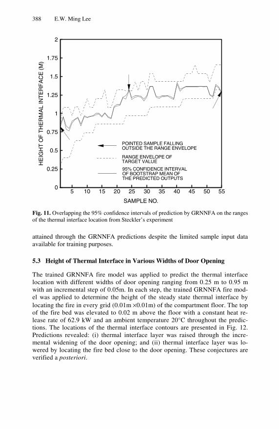
388 E.W. Ming Lee
Fig. 11. Overlapping the 95% confidence intervals of prediction by GRNNFA on the ranges of the thermal interface location from Steckler’s experiment
attained through the GRNNFA predictions despite the limited sample input data available for training purposes.
5.3 Height of Thermal Interface in Various Widths of Door Opening
The trained GRNNFA fire model was applied to predict the thermal interface location with different widths of door opening ranging from 0.25 m to 0.95 m with an incremental step of 0.05m. In each step, the trained GRNNFA fire mod-el was applied to determine the height of the steady state thermal interface by locating the fire in every grid (0.01m ×0.01m) of the compartment floor. The top of the fire bed was elevated to 0.02 m above the floor with a constant heat re-lease rate of 62.9 kW and an ambient temperature 20°C throughout the predic-tions. The locations of the thermal interface contours are presented in Fig. 12. Predictions revealed: (i) thermal interface layer was raised through the incre-mental widening of the door opening; and (ii) thermal interface layer was lo-wered by locating the fire bed close to the door opening. These conjectures are verified a posteriori.
SAMPLE NO.
HE
IGH
TO
FT
HE
RM
AL
INT
ER
FA
CE
(M)
5 10 15 20 25 30 35 40 45 50 550
0.25
0.5
0.75
1
1.25
1.5
1.75
2
95% CONFIDENCE INTERVALOF BOOTSTRAP MEAN OFTHE PREDICTED OUTPUTS
RANGE ENVELOPE OFTARGET VALUE
POINTED SAMPLE FALLINGOUTSIDE THE RANGE ENVELOPE

Application of Artificial Neural Network to Fire Safety Engineering 389
(a) Door width = 0.25m (b) Door width = 0.45m
(a) Door width = 0.65m (b) Door width = 0.85m
Fig. 12. Contours of height of thermal interface with various widths of the door opening
From a theoretical standpoint, the empirical relationships applicable for a single compartment fire could be applied to provide some significant trends thereafter confirming the thermal interface behavior predicted by the GRNNFA. Three ar-guments to the conjecture (i) are presented. The first argument focuses on the temperature of the hot gases upper layer, which can be determined by [55]:
1.63 / /(23)
where and are the gravitational acceleration and convective heat transfer coefficient of the compartment walls and ceiling. The other variables as shown in Eq. (14) to (16) are depicted in Fig. 13.
0.85
0.85 0.85
0.9
0.9
0.90.95
0.95
0.95
0.95
1
11
1
1
1.05
1.05
1.05
1.05
1.05
1.1
1.1
1.1
1.1
1.1
1.15
1.15
1.15
1.15
1.1
1.2
1.2
1 .2
1.2
1 .2
1.2
1.25
1.25
1.25
1.25
1.25
1.25
1.3
1.3
1.3
1.3
Parallel distance from center of opening (m)
Per
pend
icul
ardi
stan
cefr
omce
ntre
ofop
enin
g(m
)
-1 -0.5 0 0.5 1
0.5
1
1.5
2
2.5
0.9 0.9
0.9
5
0.95 0.95
0.95
1
1
1
1
1.0
5
1.05
1.051.05
1.05
1.1
1.1
1.1
1.11.1
1.1
1 .1
5
1.1
5
1.15
1.15
1.15
1 .15
1.2
1.2
1.2
1.2
1.2
1.2
1.25
1.25
1 .2
5
1.25
1.2 5
1.3
1.3
1.3
.3
1.3
1.3
Parallel distance from center of opening (m)
Per
pend
icul
ardi
stan
cefr
om
cent
reo
fope
ning
(m)
-1 -0.5 0 0.5 1
0.5
1
1.5
2
2.5
95
0.95
0.95
1
1
1
11.05
1.05
1.05
1.05
1.1
1.1
1.1
1.1
1.1
1 .1 5
1 .15
1.15
1.15
1.151.1
1.2
1 .2
1.2
1.2
1. 2
1 .25
1.25
1.25
1.25
1.25
1.3
1.3
1.3
1.3
1.35
1.35
1.35
Parallel distance from center of opening (m)
Per
pend
icul
ardi
stan
cefr
omce
ntre
ofo
peni
ng(m
)
-1 -0.5 0 0.5 1
0.5
1
1.5
2
2.5
1
1 1
11.05
1.05
1.05
1.05
1.1
1.1
1.1
1.1
1. 1
1.1
51.
15
1.15
1.15
1.151
. 1
1.2
1.2
1.2
1.2
1.2
1.25
1.2
5
1.2
5
1.25
1.25
1.25
1.3
1. 3
1.3
1. 3
1.3
5
1.3
5
1.35
1.35
Parallel distance from center of opening (m)
Per
pend
icul
ardi
stan
cefr
om
cent
reo
fope
ning
(m)
-1 -0.5 0 0.5 1
0.5
1
1.5
2
2.5

390 E.W. Ming Lee
Fig. 13. Nomenclatures of variables shown in equation (23) to (25)
If the width of the opening (i.e. / ) is increased in Eq. (14), taking the consid-eration for a constant heat release rate and all the thermophysical properties and ambient quantities are assumed to be known, Eq. (14) yields lower steady state temperatures of the hot gases layer, , which will eventually raise the level of the neutral plane. Subsequently, the second argument to the conjecture can be shown that by considering the following relationship where the neural plane location [56] expressed by: 11 1 / / / (24)
where / is the stoichiometric fuel/air mass ratio. It can be observed from Eq. (24) that the neutral plane will be raised by the increase in the density of the hot gases. Since the value of is inversely proportional to , it can be demonstrated by combining Eqs. (23) and (24) that the neural plane will be raised by enlarging the width of the opening. The third can be argued that if the relation between the neutral plane and thermal interface locations given by Karlsson and Quintiere [57] is used:
/ 2 / (25)
The thermal interface height monotonically increases with the height of the neutral plane . It can therefore be sufficiently concluded from these three sup-porting arguments that the height of the thermal interface will rise by increasing

Application of Artificial Neural Network to Fire Safety Engineering 391
the width of the door opening for the single compartment fire thereby verifying the GRNNFA predictions.
From a numerical standpoint, we applied a well-established field model – Fire Dynamics Simulator (FDS) [53] to verify the conjecture (ii) in addition to the theoretical consideration mentioned above. In the fire simulations by FDS, the grids are evenly distributed over the whole domain with size (approx. 0.05m) which is less than the characteristic length scale [54] of the model (i.e. 0.32m). Fig. 14 represents the predicted temperature contours and velocity plots at the center section of the compartment with the fire located in the proximity of the door opening and on the back wall of the compartment respectively.
Fig. 14. Temperature profiles of the compartment fire with different fire locations
The results clearly demonstrate that the thermal interface height is lowered when the fire is near the door opening. An important insight through the vector plots shown in Fig. 14 (c) and (d) were the strong up-flow of the fire plume re-stricted the upper layer gases flowing out of the compartment for the scenario
HORIZONTAL DISTANCE FROM BACK WALL (M)
VE
RT
ICA
LD
IST
AN
CE
FR
OM
FLO
OR
(M)
0 1 2 3 40
1
2
3
45 55 66 80 96 116 140 169 204 247 298 359 434 524 633
deg C
HORIZONTAL DISTANCE FROM BACK WALL (M)
VE
RT
ICA
LD
IST
AN
CE
FR
OM
FLO
OR
(M)
0 1 2 3 40
1
2
3
45 55 66 80 96 116 140 169 204 247 298 359 434 524 633
deg C
HORIZONTAL DISTANCE FROM BACK WALL (M)
VE
RT
ICA
LD
IST
AN
CE
FR
OM
FLO
OR
(M)
0 1 2 3 40
1
2
3
1 M/S
HORIZONTAL DISTANCE FROM BACK WALL (M)
VE
RT
ICA
LD
IST
AN
CE
FR
OM
FLO
OR
(M)
0 1 2 3 40
1
2
3
1 M/S
(a) Temperature contour with fire-bed located near to the door
(b) Temperature contour with fire-bed located away from the door
(c) Velocity plot with fire-bed located near to the door
(d) Velocity plot with fire-bed located away from the door

392 E.W. Ming Lee
where the fire was located close to the door opening. This behaviour corresponded to the thermal interface captured by the GRNNFA fire model.
6 Conclusions
The GRNNFA is a novel hybrid neural network model particularly designed for noisy data regression. It employs the FA as a preprocessor as the GRNN to com-press all training samples into a set of representative kernels. The compression scheme was developed to convey the information from the prototypes of the FA to the kernels of the GRNN. This compression scheme also facilitates the noise re-moval. A heuristic algorithm was also developed for tuning the kernel widths dynamically during the course of network training.
The GRNNFA was applied to predict the locations of the thermal interfaces in single compartment fires. The predicted results were compared with the experi-mental results. It was found that the GRNNFA was able to predict the locations of the thermal interfaces well within the range envelop of the experimental results up to 94.5% accuracy (i.e. only 3 out of 55 samples was predicted outside the range envelop). It can be concluded that the GRNNFA is able to capture the behavior of the fire dynamic system from the experimental data. Also, the GRNNFA fire model is able to capture the fire phenomena from the available experimental data that the height of the thermal interface will be lowered if the width of the opening is decreased. Also, the height will also be lowered if the fire is located near to the opening of which the size is fixed. The contour plots as shown in Fig. 14 (a) and (b) are extremely useful to understand the thermal interface behavior which would require lengthy computational times for CFD models to evaluate. Also, the trained GRNNFA model was applied to the five test cases which do not appear in Steck-ler’s experiment. The results were compared with those simulated using FDS. It was found that the difference between the predictions and simulations are well within the minimum error range as shown in [52]. This test demonstrates the ex-cellent performance of the GRNNFA model in predicting the thermal interface at the unseen locations in network training. It also reveals that the prediction accura-cy is related to the amount of knowledge provided for network training which is similar to human learning.
This study demonstrates successfully that the unique, new and novel GRNNFA fire model is smart and intelligent enough to eliminate noise and uncertainties embedded in the training data sets and to capture efficiently the genuine, predomi-nant characteristics of the fire phenomena within seconds from limited samples.
References
1. Specht, D.F.: A General Regression Neural Network. IEEE Transactions on Neural Network 2(6), 568–576 (1991)
2. Rzempoluck, E.J.: Neural Network Classification of EEG During Camouflaged Object Identification. International Journal of Medical Informatics 44, 169–175 (1997)

Application of Artificial Neural Network to Fire Safety Engineering 393
3. Schaffner, C., Schroder, D.: An Application of General Regression Neural Network to Nonlinear Adaptive Control. In: Fifth European Conference on Power Electronics and Applications, vol. 4, pp. 219–224 (1993)
4. Hyun, B.G., Nam, K.: Faults Diagnoses of Rotating Machines by Using Neural Nets: GRNN and BPN. In: Proceedings of the 1995 IEEE IECON 21st International Confe-rence on Industrial Electronics, Control, and Instrumentation, vol. 2, pp. 1456–1461 (1995)
5. Leung, M.T., Chen, A.S., Daouk, H.: Forecasting Exchange Rates Using General Re-gression Neural Networks. Computers & Operations Research 27, 1093–1110 (2000)
6. Parzen, E.: On Estimation of a Probability Density Function and Mode. Ann. Math. Statist. 33, 1065–1076 (1962)
7. Grossberg, S.: Adaptive Pattern Recognition and Universal Recoding II: Feedback, Expectation, Olfaction and Illusions. Biological Cybernetics 23, 187–202 (1976)
8. Kosko, B.: Fuzzy Entropy and Conditioning. Inform. Sci. 40, 165–174 (1986) 9. Brezmes, J., Llobet, E., Vilanova, X., Orts, J., Saiz, G., Correig, X.: Correlation Be-
tween Electronic Nose Signals and Fruit Quality Indicators on Shelf-life Measure-ments with Pinklady Apples. Sensors and Actuators B 80, 41–50 (2001)
10. Araujo, R., Almeida, T.D.: Learning Sensor-based Navigation of a Real Mobile Robot in Unknown Worlds. IEEE Transaction on Systems, Man and Cybernetics – Part B 29(2), 164–178 (1999)
11. Araujo, R., Almeida, A.T.D.: Fuzzy ART Based Approach for Real-time Map Build-ing. In: Proceedings of the 5th International Workshop on Advance Motion Control, AMC 1998-Coimbra, pp. 623–628 (1998)
12. Cinque, L., Foresti, G.L., Gumina, A., Levialdi, S.: A modified Fuzzy ART for image segmentation. In: Proceedings of the 11th International Conference on Image Analysis and Processing, pp. 102–107 (2001)
13. Park, S.: Neural networks and customer grouping in e-commerce: a framework using fuzzy ART. In: Proceedings of Academia/Industry Working Conference on Research Challenges, pp. 331–336 (2000)
14. Lee, E.W.M., Lim, C.P., Yuen, R.K.K., Lo, S.M.: A hybrid neural network model for noisy data regression. IEEE Transactions on Systems, Man and Cybernetics – Part B 34(20), 951–960 (2004)
15. Yuen, R.K.K., Lee, E.W.M., Lim, C.P., Cheng, G.W.Y.: Fusion of GRNN and FA for online noisy data regression. Neural Processing Letters 19(3), 227–241 (2004)
16. Kohonen, T.: The Self-Organizing Map. Proceedings of the IEEE 78(9), 1464–1480 (1990)
17. Bezdek, J.B.: A Convergence Theorem for the Fuzzy ISODATA Clustering Algo-rithms. IEEE Trans. Pattern Anal. Machine Intell. PAMI 2, 1–8 (1980)
18. Carpenter, G.A., Grossberg, S., David, B.R.: Fuzzy ART: Fast Stable Learning and Categorization of Analog Patterns by an Adaptive Resonance System. Neural Net-works 4, 759–771 (1991)
19. Lim, C.P., Harrison, R.F.: An Incremental Adaptive Network for On-line Supervised Learning and Probability Estimation. Neural Networks 10(5), 925–939 (1997)
20. Tomandl, D., Schober, A.: A Modified General Regression Neural Network (MGRNN) with New, Efficient Training Algorithms as a Robust ‘Black Box’ Tool for Data Analysis. Neural Network 14, 1023–1034 (2001)
21. Specht, D.F.: Enhancements to Probabilistic Neural Network. In: International Joint Conference on Neural Network, IJCNN, vol. 1, pp. 761–768 (1992)

394 E.W. Ming Lee
22. Burrascano, P.: Learning Vector Quantization for the Probabilistic Neural Network. IEEE Transaction on Neural Networks (2), 458–462 (1991)
23. Tseng, M.L.: Integrating Neural Networks with Influence Diagrams for Multiple Sen-sor Diagnostic Systems. Ph.D. Dissertation, University of California, Berkeley (1991)
24. Traven, H.G.C.: A Neural Network Approach to Statistical Pattern Classification by ‘Semiparametric’ Estimation of Probability Density Functions. IEEE Transactions on Neural Network 2, 366–377 (1991)
25. Bishop, C.M.: Neural Networks for Pattern Recognition. Clarendon Press, Oxford (1998)
26. Efron, B.: Bootstrap Methods: Another Look at the Jackknife. The Annals of Statis-tics 7, 1–26 (1979)
27. Efron, B.: Nonparametric Standard Errors and Confidence Intervals. The Canadian Journal of Statistics 9, 139–172 (1981)
28. Williamson, J.R.: Gaussian ARTMAP: A Neural Network for Fast Incremental Learn-ing of Noisy Multidimensional Maps. Neural Networks 9(5), 881–897 (1996)
29. Carney, J., Cunningham, P.: Tuning diversity in bagged ensembles. International Jour-nal of Neural Systems 10(4), 267–279 (2000)
30. Breiman, L.: Bagging Predictors. Technical Report no. 421, Department of Statistic, University of California at Berkeley, California (1994)
31. Friedman, J.: Multivariate Adaptive Regression Splines (with discussion). Annals of Statistics 19, 1–141 (1991)
32. Weigend, A.S., Gersehnfield, N.A.: Time Series Prediction: Forecasting the Future and Understanding the Past. Addison-Wesley, Reading (1994)
33. Singh, S.: Noise Impact on Time-series Forecasting Using an Intelligent Pattern Matching Technique. Pattern Recognition 32, 1389–1398 (1999)
34. Weiss, S.M., Kulikowski, C.A.: Computer Systems That Learn: The Classification and Prediction Methods from Statistics, Neural Nets, Machine Learning, and Expert Sys-tems. Morgan Kaufmann Publishers Inc., San Mateo (1991)
35. Beard, A.N.: Fire Models and Design. Fire Safety Journal 28, 117–138 (1997) 36. Yeoh, G.H., Yuen, R.K.K., Lee, E.W.M., Cheung, S.C.P.: Fire and Smoke Distribu-
tion in Two-room Compartment Structure. International Journal of Numerical Methods for Heat and Fluid Flow 12(2-3), 178–194 (2002)
37. Yeoh, G.H., Yuen, R.K.K., Chen, D.H., Kwok, W.K.: Combustion and Heat Transfer in Compartment Fires. Numerical Heat Transfer Part A-Applications 42(1-2), 153–172 (2002)
38. Yeoh, G.H., Yuen, R.K.K., Lo, S.M., Chen, D.H.: On Numerical Comparison of En-closure Fire in a Multi-compartment Building. Fire Safety Journal 38, 85–94 (2003)
39. Chen, Y., Sathyamoorthy, S., Serio, M.A.: New Fire Detection System Using FT-IR Spectroscopy and Artificial Neural Network. NISTIR6242. In: NIST annual confe-rence fire research Gaithersburg, MD (November 1998)
40. Ishii, H., Ono, T., Yamauchi, Y., Ohtani, S.: Fire Detection System by Multi-layered Neural Network with Delay Circuit. In: Fire Safety Science – Proceedings of the fourth international symposium on Fire Safety Science, pp. 761–772 (1994)
41. Milke, J.A., Mcavoy, T.J.: Analysis of Signature Patterns for Discriminating Fire De-tection with Multiple Sensors. Fire Technology 31(2), 120–136 (1995)
42. Okayama, Y.: A Primitive Study of a Fire Detection Method Controlled By Artificial Neural Net. Fire Safety Journal 17(6), 535–553 (1991)
43. Pfister, G.: Multisensor / Multicriteria Fire Detection: A New Trend Rapidly Becomes State of Art. Fire Technology 33(2), 115–139 (1997)

Application of Artificial Neural Network to Fire Safety Engineering 395
44. Lee, W.M., Yuen, K.K., Lo, S.M., Lam, K.C.: Prediction of Sprinkler Actuation Time Using the Artificial Neural Networks. Journal of Building Surveying 2(1), 10–13 (2000)
45. Lee, E.W.M., Yuen, R.K.K., Lo, S.M., Lam, K.C.: Application of Fuzzy ARTMAP for Prediction of Flashover in Compartmental Fire. In: Proceedings of International confe-rence on Construction, Hong Kong, June 19-21, pp. 301–311 (2001)
46. Lee, E.W.M., Yuen, R.K.K., Lo, S.M., Lam, K.C.: Probabilistic Inference with Maxi-mum Entropy for Prediction of Flashover in Single Compartment Fire. Advanced En-gineering Informatics 16(3), 179–191 (2002)
47. Lee, E.W.M., Yuen, R.K.K., Lo, S.M., Lam, K.C., Yeoh, G.H.: A Novel Artificial Neural Network Fire Model for Prediction of Thermal Interface Location in Single Compartment Fire. Fire Safety Journal 39(1), 67–87 (2004)
48. Yuen, R.K.K., Lee, E.W.M., Lo, S.M., Yeoh, G.H.: Prediction of Temperature and Ve-locity Profiles in a Single Compartment. Fire by an Improved Neural Network Analy-sis 41(6), 478–485 (2006)
49. Lee, E.W.M., Lee, Y.Y., Lim, C.P., Tang, C.Y.: Application of a Noisy Data Classifi-cation Technique to Determine the Occurrence of Flashover in Compartment Fires. Advanced Engineering Informatics 20(2), 213–222 (2006)
50. Lee, E.W.M., Lau, P.C., Yuen, K.K.Y.: Application of Artificial Neural Network to Building Compartment Design for Fire Safety. In: Corchado, E., Yin, H., Botti, V., Fyfe, C. (eds.) IDEAL 2006. LNCS, vol. 4224, pp. 265–274. Springer, Heidelberg (2006)
51. Lee, E.W.M.: Application of an Intelligent Model Developed from Experimental Data to Building Design for Fire Safety. Stochastic Environmental Research and Risk As-sessment 23(4), 493–506 (2009)
52. Steckler, K.D., Quintiere, J.D., Rinkinen, W.J.: Flow induced by fire in a compart-ment. NBSIR 82-2520, National Bureau of Standards, Washington D.C. (1982)
53. McGranttan, K.B., Baum, H.R., Rehm, R.G., Hamins, A., Forney, G.P.: Fire Dynam-ics Simulator – Technical Reference Guide NISTIR 6467. National Institute of Stan-dards and Technology, Gaithersburg, MD (2000)
54. Wang, H.Y., Coutin, M., Most, J.M.: Large-eddy-simulation of Buoyancy-driven Fire Propagation Behind a Pyrolysis Zone Along the Vertical Wall. Fire Safety Journal 37, 259–285 (2002)
55. McCaffrey, B.J., Quintiere, J.G., Harkleroad, M.F.: Estimating Room Temperatures and the Likelihood of Flashover Using Fire Test Data Correlations. Fire Technolo-gy 17, 98–119 (1982)
56. Drysdale, D.: An Introduction to Fire Dynamics. John Wiley and Sons, Chichester (1996)
57. Karlsson, B., Quintiere, J.: Enclosure Fire Dynamics. CRC Press LLC, Boca Raton (2000)


L.C. Jain and C.P. Lim (Eds.): Handbook on Decision Making, ISRL 4, pp. 397–425. springerlink.com © Springer-Verlag Berlin Heidelberg 2010
Chapter 16
Decision-Making for the Optimal Strategy of Population Agglomeration in Urban Planning
with Path-Converged Design
Bing Xu1,2 and Junzo Watada2
1 Research Institute of Quantitative Economics, Zhejiang Gongshang University, Hang Zhou, China
2 Graduate School of Information Production & Systems, Waseda University Kita-Kyushu, Japan
Abstract. The chapter aims first to identify existing population agglomeration and its efficiency, and second to simulate decision-making for the optimal migration strategy in urban planning to eliminate inefficiency among cities in China. First, identification based on path-converged design reveals inefficiency in existing population agglomeration in China because the population mostly agglomerates to cities with urbanization levels lower than 0.35 and the population gathers into areas with urbanization levels lower than the average level in large, medium and small cities from both regional and urban perspectives. Second, decision-making for regional population migration performs well in eliminating inefficiency. By emigrating about 14, 10, and 14 percents of the regional population from cities at low urbanization levels to cities at higher urbanization levels, inefficiency strengths between benchmark and regional population distributions shrink to 0.058, 0.041, and 0.056 from 0.1464, 0.0985, 0.1397 for small, medium, and large cities, respectively.
Keywords: Population agglomeration, Inefficiency, Urbanization level, Path identification.
1 Introduction
Previous studies on urbanization have focused on population migration. Johnson [4] estimated about 39.7 million immigrations and 16.3 million emigrations in Chinese provinces during 2000. Yang [11] studied the scale and intensity of Chinese population migration and found that about 20 million rural people immigrated into the cities during 1955-2000. Yu and Zhang [12] employed related methods of direction and distance in spatial statistics to study the population immigration of Beijing, Tianjin and Tang metropolis area, Yangtze Delta metropolis area and Pearl River Delta metropolis area from the perspectives of immigration direction,

398 B. Xu and J. Watada
immigration distance and immigration factors. Wang and Huang [13] discovered that provincial immigration was an irreplaceable factor for pushing the development in Eastern China during 1995-2000.
In addition to investigations of population migration, studies tend to explore whether urbanization lags behind economic growth. Cai [1] contends that urbanization progress tends to bring about production agglomeration rather than population agglomeration, i.e., the system itself partly causes urbanization development to lag behind economic growth. The current crisis that Chinese urbanization development faces is fundamentally a systematic supply crisis [2]. Using provincial panel data during 1987-2004, Lu and Chen [8] showed that the widening income gap between urban and rural areas was related to policies favoring urban areas of the regional government.
In contrast to previous studies that focused on how to control free migration and whether urbanization lags behind economic growth in China, the objectives of this study are two-fold. First, the study aims to identify existing population agglomeration for small, medium, and large cities from both regional and urban perspectives and to evaluate the efficiency of existing population agglomeration in urban planning. Second, the study aims to propose decision-making for the optimal strategy of population agglomeration in urban planning.
Inspired by Henderson’s [3] investigation of how a significant deviation from any optimal degrees of urban concentration or rates of urbanization causes economic losses in terms of the maximization of productivity growth, this study develops a path-converged design based on a nonparametric kernel density distribution approach to identify population agglomeration and to propose decision-making for population agglomeration with the aim of eliminating inefficiency in China.
Section 2 briefly illustrates the path-converged design based on a nonparametric approach. Section 3 presents the data sources, the benchmark, and population path identification via kernel density function. Section 4 presents the decision-making for optimal population migration aiming to eliminate inefficiency. Section 5 concludes.
2 Path-Converged Design
Path-converged design identification based on nonparametric econometrics is developed in this study rather than the typical linear regression, Granger cointegration, and ARCH models. China’s population policy has caused a great disparity between the actual urban population and the registered urban population, according to household register system. For example, the floating population in Beijing is 3.573 million; 23 percents of those people were permanent 2005, and 38.8 percents of those people had worked and lived in Beijing for more than five years. They are essentially “Beijing residents.” Moreover, the statistical standard has experienced several changes and adjustments, so the observation of population data tends to vary for many reasons. The urbanization level of observed data from

Decision-Making for the Optimal Strategy of Population Agglomeration 399
the household register system deviates substantially from the actual urbanization level. Even if cross-sectional or time series data are accepted by unit root tests, the analysis of models such as linear regression and ARCH are doubtful because the distribution itself presents a fat-tail feature, and higher order moment does not exist.
The identification approach of population agglomeration originates from the change of urbanization structure with following three processes. First, suppose the initial population allocation is equilibrium of urbanization structure. Second, when new populations immigrate into the initial equilibrium, the initial structure will change to a dynamic disequilibrium of population allocation. Finally, the disequilibrium structure will revert to re-equilibrium after some time to adjust the disequilibrium into equilibrium state of resource allocation.
The first process concerned is how to model the initial equilibrium of population allocation of urbanization structure. This study starts the analysis of urbanization structure using nonparametric kernel density estimation. The initial equilibrium of urbanization structure is an unknown underlying structure, which needs to be estimated.
The second process involved is how to model the changing process of population allocation of urbanization structure from the initial equilibrium to disequilibrium, when new population immigration takes place and changes efficiency. Suppose that the total immigration is relatively small compared to the total original population. Otherwise, the initial equilibrium of urbanization structure will be broken rather than changing into a dynamic disequilibrium, which is beyond the scope of this study. Thus, the new migration population factor is not in an equivalent position as the original population. The influx of new population tends to contribute to efficiency via quality promotion rather than increase in quantity. In this sense, this study seeks to identify how the efficiency of population allocation changes under a conditional structure of the new population factor.
The final process concerned is how to model the changing process of the structure of population allocation from disequilibrium to final equilibrium. The entire process of change, from equilibrium to disequilibrium and then to final equilibrium during all periods, is due to the migration of new population immigration. To reach the goal, a path-converged design of the new population is proposed in order to identify the population allocation efficiency with the given three steps.
Suppose an underlying structure generates the observed real-world urbanization level. The identification refers to the inferences drawn from the probability distribution of the observed variables to an underlying structure. Let iX , 1, ,i n= , be the observed urbanization level of city i , suppose the underlying structure of the overall urbanization level is:
0S : ( , )f x X (1)
where ( )1 2, , , nX X X X= .

400 B. Xu and J. Watada
2.1 Benchmark Model
The estimation of the underlying structure of urbanization is given by following kernel density estimation:
1S : 1
1
1( , )
ni
ni
x Xf x X h K
n h−
=
−⎛ ⎞= ⎜ ⎟⎝ ⎠
∑ (2)
where ( )K • stands for the kernel function and h the bandwidth.
Equation (2) presents an estimation of urbanization level distribution density with combination of information in all prefecture-level cities. It gives the equal weight 1 n at each observation iX . That is, the arithmetical average weighted kernel density estimation models the equilibrium of resource allocation on overall urbanization level.
2.2 Path Model
Population migration reflects the institutional variable and is taken as a possible strategy to change the urbanization level in this study. To identify population allocation in different regions, the conditional kernel density approach is provided with a path-converged design to explore underlying structure of the urbanization level.
a) Conditional structure The estimation of the conditional density function of the conditional structure is
given by:
2S :( , )
( , | )( )
nn
n
f x pf x X p
f p=
20
1
11
1
1,
1
nl l
ln
j
j
x X p ph K
n h hp p
h Kn h
−
=
−
=
− −⎛ ⎞⎜ ⎟⎝ ⎠=
−⎛ ⎞⎜ ⎟⎝ ⎠
∑
∑ (3)
Taking
0 1,l l l lx X p p p p x XK K K
h h h h
− − − −⎛ ⎞ ⎛ ⎞ ⎛ ⎞=⎜ ⎟ ⎜ ⎟ ⎜ ⎟⎝ ⎠ ⎝ ⎠ ⎝ ⎠
Let

Decision-Making for the Optimal Strategy of Population Agglomeration 401
1
11
l
l nj
j
p pK
hp p
Kh
ω
=
−⎛ ⎞⎜ ⎟⎝ ⎠=
−⎛ ⎞⎜ ⎟⎝ ⎠
∑ (4)
Here 0 1,K K and h are the same kernel function and bandwidth in equation (2), and
iω is a path of the population weight of city i , 1, ,i n= . i ip p t=() is designed according to the ratio of population to GDP for city i at time t .
Therefore, the conditional density function of the conditional structure is given by:
1
1
( ) ( | )n
in n j
j
x Xf x X f x X p h K
hω ω −
=
−⎛ ⎞= = ⎜ ⎟⎝ ⎠
∑, , ,
(5)
Suppose that 1/j nω = defines the equilibrium of population allocation in relationship (4) among all cities; then jω in (5) is an indicator of the degree of disequilibrium of population allocation. The value jω represents the strength of the disequilibrium. This is indispensable to the path-converged design because it describes the declining efficiency of new population immigration over time.
b) Path-converged design
In particular, let ( )1l
l
p p 1K I p p h
h 2h
−⎛ ⎞ = − ≤⎜ ⎟⎝ ⎠
, then
1
11
1l
l nj
j
p pK
hp p n
Kh
ω
=
−⎛ ⎞⎜ ⎟⎝ ⎠= =
−⎛ ⎞⎜ ⎟⎝ ⎠
∑
(6)
With the uniform density function1K , without revealed efficiency of population,
equation (6) makes model (5) back to model (2). With the uniform density function
1K , equation (6) turns model (5) back into
model (2). Now let
( )1l l
l
p p pK I p p h
h 2h
−⎛ ⎞ = − ≤⎜ ⎟⎝ ⎠
in (5), then
1
11
l
l nj
j
p pK
hp p
Kh
ω
=
−⎛ ⎞⎜ ⎟⎝ ⎠=
−⎛ ⎞⎜ ⎟⎝ ⎠
∑1
ln
lj
p
p=
=∑
(7)

402 B. Xu and J. Watada
Furthermore, the economic assumption that /l l lp t P t GDP t=() () () will converge to
a constant as time t approaches infinity and the probability one holds true,
( )lim 1l
t
P t constantp→∞
= =() (8)
Even if time t is given, equation (8) still may hold true because of the effect of planned economy on GDP and the effect of the household register system on population in China.
Then:
lim 0 11
tlP t
nω
→∞= =⎡ ⎤⎛ ⎞−⎜ ⎟⎢ ⎥⎝ ⎠⎣ ⎦
() (9)
This equation is referred to as the lω path-converged design in this study.
Now the Path identification of underlying structures is given as follows.
Definition 1. The underlying structure 0S is said to be ω path identifiable with probability one if (9) and both equations (10) and (11) are satisfied:
(a) ( )lim ( , ) ( , ) 1nnP f x X f x X
→∞= =
(10)
(b) [ ]( )lim ( , , ) ( , ) 0 1n nn
P f x X f x Xω→∞
− = = (11)
The population path identification realizes the identification of changes in allocation efficiency of population path ω and the identification of the urbanization underlying structure
0S of production efficiency by observing the changes in the efficiency of path model
2S based on benchmark model 1S with probability one.
Definition 2. City x is said to be inefficient if the underlying structure 0S is ω path identifiable, and x satisfies ( , , ) ( , )n nf x X f x Xω < . Furthermore, the ω inefficient interval is comprised of all inefficient points; i.e, inefficient interval
{ }:D x x is ineficiency= .
Definition 3. The strength of ω path inefficiency is defined by the integral area between the benchmark density function and the path density function at an
inefficiency interval, i.e, D
( ( , ) ( , , ))n nf x X f x X dxω ω−∫ , if the city x is ω
allocation inefficient. Xu and Watada [14] proved in 2008 that underlying path 0S is identifiable with
probability one, that is, underlying path 0S is identified by the difference between benchmark path 1S and factor path 2S via probability.
The choice of kernel function ( )K • and bandwidth h is of crucial importance for both benchmark and population path distribution. The kernel function in this
research is a Gauss kernel function: 1/ 2 2
1( ) (2 ) exp( / 2)K u uπ −= − .

Decision-Making for the Optimal Strategy of Population Agglomeration 403
Because h is related to corresponding weights in the study, conventional
bandwidth selection methods irrelevant to jϖ and j are inappropriate. This study
tries to obtain the bandwidth through the following steps. The choice of bandwidth h determines the amount of smoothing needed to
estimate kernel density. Inspired by the application of Maria and Roberto [9], we define the number of modes of weighted density ( )f xω as:
' ''( ) #{ : ( ) 0 ( ) 0}M f y f y and f yω ω ω+= ∈ ℜ = <
Null hypothesis 0H : the underlying density fω has m modes ( ( )M f mω ≤ );
1H : fω has more than m modes ( ( )M f mω > )
for 1, ,m M= … , where ˆhfω is the weighted kernel density estimate and h the
overall bandwidth. Bootstrap multimodality test is based on the notions of critical smoothing and
critical bandwidth. The m th− critical bandwidth ,ˆ
m crith is defined by:
,ˆ ˆinf{ : ( ) }
m crit hh h M f mω= ≤
When ,ˆm crith h= , ˆ
hfω will display m modes with a shoulder. When h further
decreases, an additional ( 1)m th+ − mode will appear in the place of the shoulder.
Thus, this study attempts to select h through following process: Step 1. Apply the Cross Validation method to the benchmark model (1) on the
rule of IMSE , and then select the initial pilot bandwidth 1h ; Step 2. For 1, ,m M= … of weighted density function ( )hf xϖ , obtain each
,ˆ
m crith . Step 3. Bootstrap test on the number of modes m , for 1, ,m M= … . (a). As suggested by Silverman [10], the bootstrap data jx are generated by:
2 2 1/ 2
, ,ˆ ˆ(1 / ) ( )j j j j
i m crit i m critx y h y y hσ ε−= + + − + (12)
where jiy are randomly drawn (with replacement) from the original sample, jy is
its mean, 2σ is its variance, and ε is an . . (0, 1)i i d N variable
for 1, ,j b= … , 1, ,i n= … ; (b). For 1, ,j b= … , apply the weighted kernel method to obtain bootstrap
estimate ,,
ˆm crit
jhf ω based on the critical bandwidth ,
ˆm crith that is computed from the
original data. For each bootstrap sample, calculate the corresponding number of modes
,,ˆ( )
m crit
j
hM fω and the m-th critical bandwidth ,ˆ jm crith .
(c). Compute the estimate of the achieved significance level (ASL) or p-value:
,1
1 ˆ#{ ( ) }m crit
bj
m m hj
A SL p M f mb =
= = >∑ (13)
(d). Do not reject the null of m modes in the underlying density if m
ASL or mp is sufficiently large.

404 B. Xu and J. Watada
The test is performed by simultaneously computing mASL for all 1, ,m M= … ,
where M is a predetermined number. For the underlying density fω , we select an
estimate m as the critical number of modes if mASL shows the largest value
among all mASL for 1, ,m M= … .
With the bandwidth h and kernel function ( )K • , the benchmark model
( )hf x , regional population path distribution 1 , ( )hf xω and urban population path
2 , ( )hf xω are obtained.
1
1
( )n
in j
j
x Xf x h K
hω ω −
=
−⎛ ⎞= ⎜ ⎟⎝ ⎠
∑ (14)
where ( )K • is a kernel function, and h is the bandwidth, 1 , ( )hf xω and
2 , ( )hf xϖ
are the regional population factor path and the urban population factor path of
urbanization level, respectively. 1 1 1
1
n
i i j
j
l lω=
= ∑ , 2 2 2
1
n
i i j
j
l lω=
= ∑ , 1 jl ,
2 jl are
the ratios of regional population, total urban population to GDP for city j, respectively.
3 Population Agglomeration Identification
3.1 Data
The data source for this study is the Chinese City Statistical Yearbook at www.bjinfobank.com. The variables included in the study are: (1) year-end total population in urban area, (2) year-end non-agriculture population in urban area, (3) year-end total population in entire city, and (4) year-end non-agriculture population in entire city, (5) GDP in urban area and (6) GDP in entire city of prefecture-level cities in 2002, 2004, and 2006. The prefecture-level cities in this study refer to all prefecture-level cities, cities at sub-provincial levels, and municipalities directly managed by the central government in China. According to the classifications in China, the entire city of the prefecture-level city is the administrative area under the city’s jurisdiction, including the countryside or numerous counties and county-level cities, and refers to the regional area in this study. The urban municipal district refers to the urban city and its suburbs, which are taken as an urban area in this study.
Two definitions are widely used to describe the development of the urbanization level: the proportion of urban population and the proportion of non-agricultural population. The first definition is usually used for the analysis of single urbanization development levels in China. In this study, non-agriculture population data for prefecture-level cities, rather than urban population data, are available. Moreover, this study seeks to obtain the overall urbanization development level

Decision-Making for the Optimal Strategy of Population Agglomeration 405
from the urbanization development levels of nearly 300 prefecture-level cities, focusing on the relativity of the data rather than the absoluteness. In this sense, the study is different from the single index of urbanization level. Accordingly, this study takes the urbanization level to be the proportion of non-agriculture population. This embodies the shift of rural surplus labor to the city and also expresses the labor receiving capability of the city. The statistical data reveal that the urbanization levels by the second definition in 2002, 2004, and 2006 are 27.89%, 30.81%, and 36.26%, respectively, which are lower than the urbanization level defined by the proportion of urban population [6].
The reason for using urbanization development in prefecture-level cities to represent the urbanization level is that China’s growth in the 1990s was sustained mainly by these cities. The total GDP of over 290 prefecture-level cities accounted for more than 50% of GDP in 2000, and their average growth rates are mostly over 12%. China might have failed to deal with deflation in the 1990s if not for the double-digit growth of the prefecture-level cities.
The current research aims to identify the existing population agglomeration and its efficiency in urban planning with the path-converged design in China. It is pursued from the following two perspectives:
The study seeks to identify population agglomeration and its efficiency in urban planning in China by using a path-converged design from the following two perspectives:
1). The perspective of city size, which separates nearly 300 prefecture-level cities in China into large, middle-sized, and small cities according to an urban population scale, which is different from the usual single urbanization level;
2). The perspective of spatial location, which separates city regions into urban and regional areas according to the scale of the city region.
3.2 Urbanization Level:Benchmark Model
Figure 1 shows the benchmark distribution of urbanization levels in prefecture-level cities in 2002, 2004, and 2006 and reflects the agglomeration level. Table 1 displays
detailed information regarding the distributions in each year. max( )hf x is the
maximum value of function ( )hf x , 1S ,
2S , and 3S are the integral values of each
distribution at the intervals (0, 0.35], (0.35, 0.7], and (0.7, 1], satisfying 0.35
1 0( )S f x dx= ∫ ,
0.7
2 0.35( )S f x dx= ∫ ,
1
3 0.7( )S f x dx= ∫ . The intervals (0, 0.35], (0.35,
0.7], and (0.7, 1] illustrate low, medium, and high urbanization levels. EX is the expected value of overall urbanization development level in China with each
distribution, satisfying 0
( )hE X x f x d x∞
= ∫ the overall average urbanization
level in each year. The bottom row in Table 1 presents the average growth rate of each index during 2002-2006 (if negative, it is declining). The average growth rate
of the expected value is 1.79%, obtained by solving 40.3145(1 ) 0.3376x+ = .
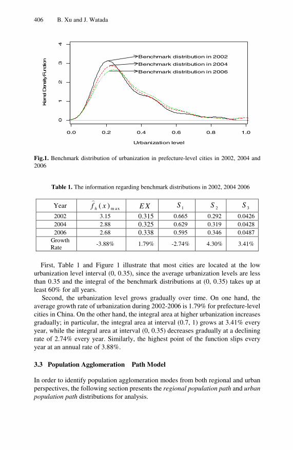
406 B. Xu and J. Watada
0.0 0.2 0.4 0.6 0.8 1.0
01
23
4
Urbanization level
Ker
nel D
ensity F
unction
Benchmark distribution in 2002
Benchmark distribution in 2004
Benchmark distribution in 2006
Fig.1. Benchmark distribution of urbanization in prefecture-level cities in 2002, 2004 and 2006
Table 1. The information regarding benchmark distributions in 2002, 2004 2006
Year m ax( )hf x E X 1S 2S 3S 2002 3.15 0.315 0.665 0.292 0.0426 2004 2.88 0.325 0.629 0.319 0.0428 2006 2.68 0.338 0.595 0.346 0.0487
Growth Rate
-3.88% 1.79% -2.74% 4.30% 3.41%
First, Table 1 and Figure 1 illustrate that most cities are located at the low urbanization level interval (0, 0.35), since the average urbanization levels are less than 0.35 and the integral of the benchmark distributions at (0, 0.35) takes up at least 60% for all years.
Second, the urbanization level grows gradually over time. On one hand, the average growth rate of urbanization during 2002-2006 is 1.79% for prefecture-level cities in China. On the other hand, the integral area at higher urbanization increases gradually; in particular, the integral area at interval (0.7, 1) grows at 3.41% every year, while the integral area at interval (0, 0.35) decreases gradually at a declining rate of 2.74% every year. Similarly, the highest point of the function slips every year at an annual rate of 3.88%.
3.3 Population Agglomeration:Path Model
In order to identify population agglomeration modes from both regional and urban perspectives, the following section presents the regional population path and urban population path distributions for analysis.

Decision-Making for the Optimal Strategy of Population Agglomeration 407
0.0 0.2 0.4 0.6 0.8 1.0
01
23
4
Urbanization level
Ker
nel D
ensity F
unctio
n Regional population path distribution in 2002
Regional population path distribution in 2004 Regional population path distribution in 2006
Fig. 2. Regional population path distributions of urbanization in prefecture-level cities in 2002, 2004 and 2006
Table 2. Regional population path distributions in 2002, 2004, 2006
Year m ax( )hf x 1E X 1S 2S 3S 2002 3.97 0.253 0.801 0.180 0.0164 2004 3.60 0.260 0.782 0.196 0.0178 2006 3.37 0.270 0.755 0.221 0.0192
Growth Rate
-4.01% 1.66% -1.48% 5.21% 4.02%
Figure 2 and Table 2 list information about the regional population path distributions, reflecting the regional population agglomeration modes of cities. The average growth rate of the average regional urbanization is 1.66% during 2002-2006. Similar to benchmark case, the integral area at higher urbanization levels increases gradually. In particular, the integral area at interval (0.7, 1) grows at 4.02% every year, while the integral area at interval (0, 0.35) decreases gradually at a rate of 1.48% every year. Again, the maximum value of the regional population path distributions slips yearly at an annual rate of 4.01%.
Figure 3 and Table 3 illustrate the details of urban population path distributions, giving detailed information on urban population agglomeration modes of cities. The average growth rate of urbanization level is 1.87% during 2002-2006. The integral area at higher urbanization increases gradually; in particular, the integral area at interval (0.7, 1) grows by 2.74% every year, while the integral area at interval (0, 0.35) decreases gradually at a rate of 1.33% every year. Again, the maximum value of the urban population path distributions decreases at an annual rate of 3.84%.

408 B. Xu and J. Watada
0.0 0.2 0.4 0.6 0.8 1.0
01
23
4
Urbanization level
Ker
nel D
ensity
Fun
ctio
n Urban population path distribution in 2002
Urban population path distribution in 2004Urban population path distribution in 2006
Fig. 3. Urban population path distributions of urbanization in prefecture-level cities in 2002, 2004 and 2006
Table 3. Urban population path distributions in 2002, 2004, 2006
Year m ax( )hf x 2E X 1S
2S 3S
2002 3.89 0.260 0.783 0.192 0.0236 2004 3.61 0.265 0.769 0.200 0.0252 2006 3.33 0.276 0.742 0.226 0.0263
Growth Rate
-3.84% 1.52% -1.33% 4.16% 2.74%
In sum, two conclusions are presented regarding the population agglomeration modes of both regional and urban perspectives.
First, both the regional and urban populations agglomerate to cities with urbanization lower than 0.35 because the integrals of both the regional population path and urban population path distributions at (0, 0.35) take up at least 75% for all years, which presents the inefficiency of population agglomeration.
Second, the agglomeration of both regional and urban populations shrinks gradually over time because the integral areas at (0, 0.35) witness a declining trend for both path distributions.
3.4 Leftward Population Agglomeration
This section aims to clarify whether the population mainly gathers into region or into urban area through the channel of urbanization level.
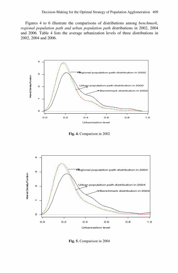
Decision-Making for the Optimal Strategy of Population Agglomeration 409
Figures 4 to 6 illustrate the comparisons of distributions among benchmark, regional population path and urban population path distributions in 2002, 2004 and 2006. Table 4 lists the average urbanization levels of three distributions in 2002, 2004 and 2006.
0.0 0.2 0.4 0.6 0.8 1.0
01
23
4
Urbanization level
Kerne
l Den
sity Fun
ction
Benchmark distribution in 2002
Regional population path distribution in 2002
Urban population path distribution in 2002
Fig. 4. Comparison in 2002
0.0 0.2 0.4 0.6 0.8 1.0
01
23
4
Urbanization level
Ker
nel D
ensity F
unction
Benchmark distribution in 2004
Regional population path distribution in 2004
Urban population path distribution in 2004
Fig. 5. Comparison in 2004

410 B. Xu and J. Watada
0.0 0.2 0.4 0.6 0.8 1.0
0.0
0.5
1.0
1.5
2.0
2.5
3.0
3.5
Urbanization level
Ker
nel D
ensi
ty F
unct
ion
Benchmark distribution in 2006
Regional population path distribution in 2006
Urban population path distribution in 2006
Fig. 6. Comparison in 2006
Table 4. The average urbanization levels of the distributions of benchmark, regional population and urban population path in 2002, 2004 and 2006
Year E X 1E X1
E X - E X 2E X 2E X - E X
2002 0.315 0.253 -0.0617 0.260 -0.0546 2004 0.325 0.260 -0.0650 0.265 -0.0601 2006 0.338 0.270 -0.0676 0.276 -0.0614 Average 0.326 0.261 -0.0648 0.267 -0.0587
where EX ,1
EX and 2
EX denote the expected values of the benchmark, regional population path, and urban population path distribution , respectively.
In Table 4, EX ,1
EX and 2
EX represent the expected values of benchmark, regional population path, and urban population path distributions , respectively.
The figures show the same trends: both the regional and urban population path distributions drift leftward based on their corresponding benchmark distribution, which hints the inefficiency of population agglomeration. The regional population path distributions experience a stronger shift compared with the urban population path distributions. This implies that both regional and urban population path distributions reduce the overall level of urbanization, which is also observed from the figures in Table 4.
The expected values of the benchmark distributions are the highest, and the expected values of regional population path distributions are the lowest. The regional population path and urban population path reduce the benchmark expected values by 6.96% and 6.27%, which are obtained by
1E X - E X and 2E X - E X ,

Decision-Making for the Optimal Strategy of Population Agglomeration 411
respectively. This result implies that the population gathers into areas with urbanization levels lower than both average regional and urban urbanization levels. However, the strength of the decline of the regional population path distribution is slightly stronger than the strength of the decline of the urban population path distribution.
3.5 Inefficiency of Population Agglomeration: City Size
The study shows in the previous section that the population mainly gathers into cities at lower urbanization levels from both regional and urban perspectives. In order to clarify whether the inefficiency of population agglomeration exists in small, medium and large cities, the research goes on to explore the agglomeration from the perspective of city size.
In this section the research separates all prefecture-level cities into three groups: small cities (total urban population less than 0.5 million), medium cities (their total urban population range from 0.5 to 1 million), and large cities (their total urban population larger than 1 million). The research gives the benchmark, regional population path and urban population path distributions for small cities, medium cities and large cities in 2000, 2002 and 2004, respectively, to identify the feature of population agglomeration. Figures 7 to 12 present the three distributions for three city groups in 2004 and 2006, and Table 5 lists their corresponding expected values.
0.0 0.2 0.4 0.6 0.8 1.0
01
23
45
Urbanization level
Ker
nel D
ensi
ty F
unct
ion
Benchmark distributionfor small cities in 2004
Regional population path distributionfor small cities in 2004
Urban population path distributiofor small cities in 2004
Fig. 7. Distributions of small cities in 2004

412 B. Xu and J. Watada
0.0 0.2 0.4 0.6 0.8 1.0
0.0
1.0
2.0
3.0
Urbanization level
Ker
nel D
ensi
ty F
unct
ion
Benchmark distributionfor medium cities in 2004
Regional population path distributionfor medium cities in 2004
Urban population path distributionfor medium cities in2004
Fig. 8. Distributions of medium cities in 2004
0.0 0.2 0.4 0.6 0.8 1.0
0.0
0.5
1.0
1.5
2.0
2.5
3.0
Urbanization level
Ker
nel D
ensi
ty F
unct
ion
Benchmark distributionfor large cities in 2004
Regional population path distributionfor large cities in 2004
Urban population path distributionfor large cities in 2004
Fig. 9. Distributions of large cities in 2004
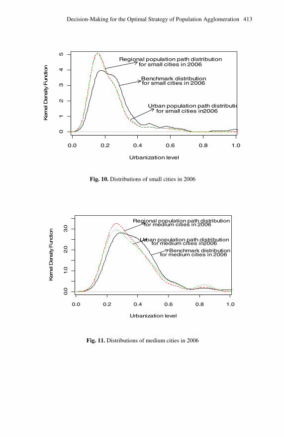
Decision-Making for the Optimal Strategy of Population Agglomeration 413
0.0 0.2 0.4 0.6 0.8 1.0
01
23
45
Urbanization level
Ker
nel D
ensi
ty F
unct
ion
Benchmark distributionfor small cities in 2006
Regional population path distributionfor small cities in 2006
Urban population path distributiofor small cities in2006
Fig. 10. Distributions of small cities in 2006
0.0 0.2 0.4 0.6 0.8 1.0
0.0
1.0
2.0
3.0
Urbanization level
Ker
nel D
ensi
ty F
unct
ion
Benchmark distributionfor medium cities in 2006
Regional population path distributionfor medium cities in 2006
Urban population path distributionfor medium cities in2006
Fig. 11. Distributions of medium cities in 2006

414 B. Xu and J. Watada
0.0 0.2 0.4 0.6 0.8 1.0
0.0
0.5
1.0
1.5
2.0
2.5
3.0
Urbanization level
Ker
nel D
ensi
ty F
unct
ion
Benchmark distributionfor large cities in 2006
Regional population path distributionfor large cities in 2006
Urban population path distributionfor large cities in2006
Fig. 12. Distributions of large cities in 2006
Table 5. The average urbanization levels of the benchmark, regional population and urban population path distributions for small cities
Year E X 1E X 2E X 2004 0.255 0.215 0.216
2006 0.260 0.219 0.222
The average urbanization levels for medium cities
Year E X 1E X
2E X
2004 0.369 0.342 0.368
2006 0.376 0.348 0.3642
The average urbanization levels for large cities
Year E X 1E X 2E X 2004 0.483 0.439 0.463
2006 0.499 0.447 0.464
where EX ,1
EX and 2
EX denote the expected value of benchmark, regional population path, and urban population path distributions, respectively.

Decision-Making for the Optimal Strategy of Population Agglomeration 415
Compared with the benchmark, both regional and urban population path distributions in each city group in all years drift leftward, which is consistent with the tendency of all prefecture-level cities. The regional population path and urban population path distributions tend to be the same for small cities in both 2004 and 2006. However, the urban population path distributions tend to shift rightward compared with the regional population path distributions for medium and large cities in both years.
The inefficiency of population agglomeration is identified in large, medium and small cities because all the population gathers into the cities whose urbanization levels are lower than the average levels from both regional and urban perspectives. More specifically, the regional population mainly gathers into the cities whose urbanization levels are lower than 0.2143 for small cities, lower than 0.3341 for medium cities and lower than 0.4919 for large cities in 2006. The urban population agglomeration is similar to the regional population agglomeration in small and large cities, while the urban population mainly gathers into the cities whose urbanization levels are lower than 0.2935 for medium cities.
With the aim to promote urbanization, population migration from cities at low urbanization levels to cities at high levels is expected to be implemented based on the identified population agglomeration modes.
4 Decision Making on Optimal Migration Strategy
Identification indicates that the existing population agglomeration is inefficient. The decision making is to induce population migration from cities at low urbanization level to cities at high urbanization level in order to eliminate inefficiency. The theoretical optimization of migration population jp for city j satisfies the equation as follows:
( ) ( ) 0j n jf x f xω − = (4.1)
where 1
1
1( )
ni
ni
x Xf x h K
n h−
=
−⎛ ⎞= ⎜ ⎟⎝ ⎠
∑ , and 1
1
( )n
ij
j
x Xf x h K
hω ω −
=
−⎛ ⎞= ⎜ ⎟⎝ ⎠
∑ .
However, it is hard to obtain the unique solution of equation (4.1). Fortunately, it is represented by
( )1
0
( ) - ( ) 0nf x f x dxω =∫ (4.2)
because the integral of probability density 1
0
( ) 1f x dxω =∫
and 1
0
( ) 1nf x dx =∫
Furthermore, population migrates from the cities at lower urbanization level to the cities at higher level. Thus, there are some values l, such that

416 B. Xu and J. Watada
( ) ( )1
0
( ) - ( ) ( ) - ( )l
n n
l
f x f x dx f x f x dxω ω=∫ ∫ (4.3)
l can be found with equation(4.3) . Thus, the optimal strategies for migration population are given in the sense of
equation (4.2) for small, medium and large cities in 2006.
4.1 Decision 1: Small Cities
l is 0.214 in the decision making of regional population migration for small cities. More specifically, the decision making of population migration for small cities is implemented with four steps.
1. The strength of the migration population is 14.64 percent.
1
0.214
0( ( ) ( )) 0.1464nf x f x dxω − =∫
2. The total number of the migration population is
1
0.1464 ( 0.214)n
k kk
p I u=
<∑
where
kp
is the regional population of small city k, and
1
( 0.214)n
k kk
p I u=
<∑ is the
total regional population of cities whose urbanization level lower than 0.214. ( 0.214) 1kI u < = , if 0.214ku < , otherwise, ( 0.214) 0kI u < = , if 0.214ku ≥ .
3. The emigration population for some small city i is given by
1
1
E1
1
( )- ( ) ( 0.214)0.1464 ( 0.214)
( )- ( ) ( 0.214)
ni n i i
i k knk
j n j jj
f x f x I up p I u
f x f x I u
ω
ω=
=
⎡ ⎤ <⎣ ⎦= × <⎡ ⎤ <⎣ ⎦
∑∑
The immigration population for some small city i is given by
1
1
I1
1
( )- ( ) ( 0.214)0.1464 ( 0.214)
( )- ( ) ( 0.214)
nn i i i
i k knk
n j j jj
f x f x I up p I u
f x f x I u
ω
ω=
=
⎡ ⎤ ≥⎣ ⎦= × <⎡ ⎤ ≥⎣ ⎦
∑∑
It illustrates that the population migration for any small city is implemented according to the difference of benchmark and original regional population path distributions. The greater the difference, the larger population migration will be.

Decision-Making for the Optimal Strategy of Population Agglomeration 417
4. The new regional population for some small city i is obtained as
1i i iE iIp p p p= − +
5. The new regional population path weight is recalculated by new path
1
n
i i jj
l lω=
= ∑ , where 1i i il p GDP= .
Five steps present the path-converged design of the new regional population path
after migration for small cities.
The migration here only concerns the interior migration among small cities. Step
4 needs to be updated for simulation if the migration is implemented among small
and large (medium) cities.
0.0 0.2 0.4 0.6 0.8 1.0
01
23
45
Urbanization level
Ker
nel D
ensi
ty F
unct
ion
Benchmark distributionfor small cities in 2006
Regional population path distributionfor small cities in 2006
Urban population path distributiofor small cities in2006
Optimal regional population path distribufor small cities in 2006
Fig. 13. New regional population path distribution for small cities in 2006
Table 6. Information regarding decision 1
Year EX1 Optimal EX1
Inefficiency strength
Optimal Inefficiency strength
2006 0.219 0.237 0.146 (0.214) 0.0585 (0.278)

418 B. Xu and J. Watada
With the implementation of decision 1 for small cities, Figure 13 and Table 6 illustrate the decision to promote urbanization for small cities in 2006. Figure 13 illustrates the rightward shift of the regional population path distribution with the decision to migrate. Table 6 shows that the inefficiency strength between the benchmark and regional population distributions shrinks to 0.0585 from 0.146and that the average urbanization level experiences a growth of 1.84 percent (0.237-0.2186). Both findings demonstrate the fact that the decision to migrate from small cities is effective.
4.2 Decision 2: Regional Migration for Medium Cities
l is 0.334 in the decision of regional population migration for medium cities.
1. The strength of the migration population is 9.85 percent.
1
1
0.3340.0985 ( ( ) ( ))nf x f x dxω= −∫
2. The total number of the migration population is
1
0.0985 ( 0.334)n
k kk
p I u=
<∑
where
kp
is the regional population of medium city k, , and
1
( 0.334)n
k kk
p I u=
<∑ is
the total regional population of medium cities whose urbanization level lower than
0.334. 3. The emigration population for some medium city i is given by
1
1
E1
1
( )- ( ) ( 0.334)0.0985 ( 0.334)
( )- ( ) ( 0.334)
ni n i i
i k knk
j n j jj
f x f x I up p I u
f x f x I u
ω
ω=
=
⎡ ⎤ <⎣ ⎦= × <⎡ ⎤ <⎣ ⎦
∑∑
The immigration population for some medium city i is given by
1
1
I1
1
( )- ( ) ( 0.334)0.0985 ( 0.334)
( )- ( ) ( 0.334)
nn i i i
i k knk
n j j jj
f x f x I up p I u
f x f x I u
ω
ω=
=
⎡ ⎤ ≥⎣ ⎦= × <⎡ ⎤ ≥⎣ ⎦
∑∑
4. The new regional population for some medium city i
1i i iE iIp p p p= − +

Decision-Making for the Optimal Strategy of Population Agglomeration 419
0.0 0.2 0.4 0.6 0.8 1.0
0.0
0.5
1.0
1.5
2.0
2.5
3.0
3.5
Urbanization level
Ker
nel D
ensi
ty F
unct
ion
Benchmark distributionfor medium cities in 2006
Regional population path distributionfor medium cities in 2006
Urban population path distributionfor medium cities in2006
Optimal regional population path distribution
for medium cities in 2006
Fig. 14. New regional population path distribution for medium cities in 2006
Table 7. Information regarding decision No.2
Year EX1 Optimal EX1
Inefficiency strength
Optimal Inefficiency strength
2006 0.348 0.362 0.0985 (0.334) 0.0412 (0.295)
With reference to the path-converged design, the implementation of decision 2 for medium cities accompanies the information in Figure 14 and Table 7. Figure 14 illustrates the rightward shift of the regional population path distribution with the decision to migrate. Table 7 illustrates the inefficiency strength between the benchmark and regional population distributions shrinks to 0.0412 from 0.0985 and the average urbanization level experiences a growth of 1.41 percents.
4.3 Decision 3: Urban Migration for Medium Cities
l is 0.294 in the decision making of urban population migration for medium cities.
1. The strength of the migration population is 7.10 percent.
2
1
0.2940.071 ( ( ) ( ))nf x f x dxω= −∫

420 B. Xu and J. Watada
2. The total number of the migration population is
1
0.071 ( 0.294)n
k kk
p I u=
<∑
where
kp
is the urban population of medium city k,
2
1
0.2940.071 ( ( ) ( ))nf x f x dxω= −∫ , and
1
( 0.294)n
k kk
p I u=
<∑ is the total urban
population of medium cities whose urbanization level lower than 0.294. 3. The urban emigration population for some medium city i is given by
2
2
E1
1
( )- ( ) ( 0.294)0.071 ( 0.294)
( )- ( ) ( 0.294)
ni n i i
i k knk
j n j jj
f x f x I up p I u
f x f x I u
ω
ω=
=
⎡ ⎤ <⎣ ⎦= × <⎡ ⎤ <⎣ ⎦
∑∑
The immigration population for some medium city i is given by
2
2
I1
1
( )- ( ) ( 0.294)0.071 ( 0.294)
( )- ( ) ( 0.294)
nn i i i
i k knk
n j j jj
f x f x I up p I u
f x f x I u
ω
ω=
=
⎡ ⎤ ≥⎣ ⎦= × <⎡ ⎤ ≥⎣ ⎦
∑∑
4. The new urban population for some medium city i
1i i iE iIp p p p= − +
The implementation of decision 3 for medium cities is presented in Figure 15 and Table 8. Figure 15 illustrates the rightward shift of urban population path distribution with the decision making on population migration. Table 8 presents the inefficiency strength between the benchmark and urban population distributions shrinks to 0.0473 from 0.071 and the average urbanization level experiences no obvious growth.
Table 8. Information regarding decision No.3
Year EX2 Optimal EX2
Inefficiency strength
Optimal Inefficiency strength
2006 0.364 0.363 0.0710(0.294) 0.0473(0.284)

Decision-Making for the Optimal Strategy of Population Agglomeration 421
0.0 0.2 0.4 0.6 0.8 1.0
0.0
0.5
1.0
1.5
2.0
2.5
3.0
3.5
Urbanization level
Ker
nel D
ensi
ty F
unct
ion
Benchmark distributionfor medium cities in 2006
Regional population path distributionfor medium cities in 2006
Urban population path distributionfor medium cities in2006
Optimal urban population path distributionfor medium cities in 2006
Fig. 15. New urban population path distribution for medium cities in 2006
4.4 Decision 4: Regional Population Migration for Large Cities
l is 0.492 in the decision of regional population migration for large cities. 1. The strength of the migration population is 14.0 percent.
1
1
0.4920.140 ( ( ) ( ))nf x f x dxω= −∫
2. The total of the migration population is
1
0.140 ( 0.492)n
k kk
p I u=
<∑
where
kp
is the regional population of large city k,
1
1
0.4920.140 ( ( ) ( ))nf x f x dxω= −∫ , and
1
( 0.492)n
k kk
p I u=
<∑ is the total regional
population of large cities whose urbanization level lower than 0.492.
3. The emigration population for some large city i is given by
1
1
E1
1
( )- ( ) ( 0.492)0.140 ( 0.492)
( )- ( ) ( 0.492)
ni n i i
i k knk
j n j jj
f x f x I up p I u
f x f x I u
ω
ω=
=
⎡ ⎤ <⎣ ⎦= × <⎡ ⎤ <⎣ ⎦
∑∑

422 B. Xu and J. Watada
The immigration population for some large city i is given by
1
1
I1
1
( )- ( ) ( 0.492)0.140 ( 0.492)
( )- ( ) ( 0.492)
nn i i i
i k knk
n j j jj
f x f x I up p I u
f x f x I u
ω
ω=
=
⎡ ⎤ ≥⎣ ⎦= × <⎡ ⎤ ≥⎣ ⎦
∑∑
4. The new regional population for some large city i
1i i iE iIp p p p= − +
0.0 0.2 0.4 0.6 0.8 1.0
0.0
0.5
1.0
1.5
2.0
2.5
3.0
Urbanization level
Ker
nel D
ensi
ty F
unct
ion
Benchmark distributiofor large cities in 2006
Regional population path distributionfor large cities in 2006
Urban population path distributionfor large cities in2006
Optimal regional population path distributionfor large cities in 2006
Fig. 16. New regional population path distribution for large cities in 2006
Table 9. Information regarding decision No.4
Year EX1 Optimal EX1
Inefficiency strength
Optimal Inefficiency strength
2006 0.447 0.474 0.140(0.492) 0.0562(0.462) The implementation of decision 4 for large cities is presented in Figure 16 and
Table 9. Figure 16 experiences the rightward shift of the regional population path distribution with the decisions for population migration. Table 9 shows that the average urbanization level experiences a growth of 2.73% and that the inefficiency strength between the benchmark and regional population distributions shrinks to 0.0562 from 0.140.

Decision-Making for the Optimal Strategy of Population Agglomeration 423
5 Conclusions
The study develops path-converged design identification based on nonparametric kernel density estimation to identify the population agglomeration and its efficiency from both regional and urban perspectives. It also proposes decisions of optimal population migration for urban planning to eliminate urbanization inefficiency in China.
5.1 Identification of Population Agglomeration
First, the identification of urbanization level with benchmark model illustrates most cities locate at the urbanization level lower than 0.35. The urbanization level grows gradually along with time because the average growth rate of urbanization level during 2002-2006 is 1.79 percent and the integral area at higher urbanization level increases gradually. In particular, the integral area at interval (0.7, 1) grows at 3.41 percent every year.
Second, the inefficiency of population agglomeration is identified for all cities in China. The identification of the population agglomeration shows that the population gathers asymmetrically around the average urbanization development level. Both regional and urban populations agglomerated to cities with urbanization levels lower than 0.35 during 2002-2006 because the integrals of both the regional population path and urban population path distributions at (0, 0.35) comprise at least 75 percents for all years. Moreover, the agglomeration of both regional and urban population shrinks gradually over time because the integral areas at (0, 0.35) experience a declining trend for both path distributions.
Third, the inefficiency of population agglomeration is also identified in large, medium and small cities. More specifically, the regional population gathers in cities with urbanization levels lower than 0.214 for small cities, lower than 0.334 for medium cities, and lower than 0.4919 for large cities in 2006. Urban population agglomeration is very similar to regional population agglomeration in small and large cities; while the urban population in medium cities gathers in cities where urbanization is lower than 0.294.
5.2 Decision Making of Optimal Population Migration
Based on the identification of population agglomeration and the inefficiency of agglomeration, four planning decisions regarding population migration are presented in order to eliminate inefficiency of population allocation.
Population migration is implemented based on the inefficiency strength of benchmark and population path distributions. The population migration number for any city is implemented according to the difference between the benchmark and original population path distributions. The greater the difference, the larger population migration will be.

424 B. Xu and J. Watada
Decision 1 for optimal regional population migration in small cities is to guide 14.64 percents of the regional population in small cities with urbanization levels lower than 0.214 to migrate to small cities at higher urbanization levels. Decision 2 for regional population migration in medium cities is to guide 9.85 percents of the regional population in the medium cities with urbanization levels lower than 0.214 to migrate to medium cities at higher urbanization levels. Decision 4 for regional population migration in large cities is to guide 14 percents of the regional population in the large cities with urbanization levels lower than 0.4919 to migrate to large cities at higher urbanization levels. The inefficiency strengths between benchmark and regional population distributions shrink to 0.058, 0.041, and 0.056 from 0.1464, 0.0985, 0.1397 respectively, and average urbanization levels with regional population path distributions experience growths of 1.84, 1.41, and 2.73 percents for small, medium and large cities respectively. All findings show that the decisions regarding regional population migration are effective.
However, the population migration this study employed is the interior migration for small, medium and large cities respectively. The path-converged design needs to be updated for simulation on migration if the population migration is implemented among different city groups, which will bring about different conclusions.
Acknowledgments. The first author is supported by the National Natural Science Foundation (No.70973110), China.
References
[1] Cai, J.: Institutional Analysis For The Lag of Urbanization Behind The Economic Development. City Planning Review 1, 67–72 (2006)
[2] Chen, Q.: Crisis And Opportunities of The Urbanization in China. City Planning Review 1, 34–39 (2006)
[3] Henderson, J.V.: The urbanization process and economic growth: the so-what question. Journal of Economic Growth 8, 47–71 (2003)
[4] Johnson, D.G.: Provincial migration in China in the 1990s. China Economic Review 14, 22–31 (2004)
[5] Li, J.W., Ji, Y.H.: International Comparison of Chinese Urbanization. Urban Development Research 3, 1–10 (2004)
[6] Li, L.J., Jin, J.: Urbanization Level Forecast Time Series model and application in China. China’s Population Science (suppl.) 1–6 (2005)
[7] Liu, W.: Eight practical issues need considering in the urbanization development. Economist 1, 77–85 (2006)
[8] Lu, M., Chen, Z.: The Economic Policy Of Urbanized, Urban Tendency and Income Difference between City and Countryside. Economic Research Journal 6, 41–49 (2004)
[9] Maria, G.P., Roberto, Z.: Testing for changing shapes of income distribution: Italian evidence in the 1990s from kernel density estimates. Empirical Economics 29, 415–430 (2004)

Decision-Making for the Optimal Strategy of Population Agglomeration 425
[10] Silverman, B.W.: Using kernel density estimates to investigate multimodality. Journal of Royal Statistical Society (B) 43, 97–99 (1981)
[11] Yang, Y.: Scale Reckoning and Strength Analysis Of Chinese Population Migration. Social Science in China 6, 97–107 (2003)
[12] Yu, L., Zhang, S.Y.: The Migration Flow and The Affecting Variables: A Case Study of the Three megalopolises of China. South China Population 3, 17–23 (2006)
[13] Wang, G.X., Huang, Y.Y.: Population Migration and Eastern Region Economic Development Of Chinese Interprovincial, 1995-2000. Population Research 1, 19–28 (2005)
[14] Xu, B., Watada, J.: The Path Identification of FDI and Financial Expenditure in China. In: Int. Symposium on Management Engineering 2008 (ISME 2008), Kitakyushu, Japan (2008)


L.C. Jain and C.P. Lim (Eds.): Handbook on Decision Making, ISRL 4, pp. 427–452. springerlink.com © Springer-Verlag Berlin Heidelberg 2010
Chapter 17
A Cognitive Interpretation of Thermographic Images Using Novel Fuzzy Learning
Semantic Memories
C. Quek1, W. Irawan1, and E. Ng2
1 Centre for Computational Intelligence, Nanyang Technological University, School of Computer Engineering, Blk N4 #2A-32,
Nanyang Avenue, Singapore 639798 2 School of Mechanical and Aerospace Engineering,
Nanyang Technological University, 50 Nanyang Avenue, Singapore 639798
Abstract. Fuzzy neural network (FNN), a hybrid of fuzzy logic and neural network, is computationally powerful, robust and able to model a complex nonlinear problem domain via the extraction and self-tuning of fuzzy IF-THEN rules. This yields a powerful semantic learning memory system that is useful to build intelligent decision support tools. Thermal imaging has been effectively used in the detection of infrared spectrum for the screening of potential SARS patients. This chapter proposes a cognitive approach in the study of the correlation and semantic interpretation of superficial thermal images against the true internal body temperature. Comparison between global and local semantic memories as well as Mamdani and TSK model of FNNs are presented. Existing infrared systems are commonly used at various boarder checkpoints and these have high false-negative rate. The use of FNN as a back-end of the system can significantly improves and hence serves the role of an intelligent medical decision support tool with high degree of accuracy. Extensive experimentations are conducted on real-life data taken from the Emergency Department (A&E), Tan Tock Seng Hospital (the designated SARS center in Singapore). The performance of FNN as the thermal analysis decision support system, providing plausible semantic interpretation and understanding, is highly encouraging.
Keywords: Semantic interpretation, learning memories, fuzzy rules, Thermal imaging, thermographs, neural fuzzy networks, intelligent decision support system, cognitive approach, brain-inspired, temperature correlation, local and global semantic networks, Mamdani and TSK models.
1 Introduction
Fuzzy systems have been developed to handle inexact information, very much similar to human reasoning, while neural networks are based on the brains

428 C. Quek, W. Irawan, and E. Ng
architecture and learning capabilities. Fuzzy neural networks (FNNs) combine the capabilities of both fuzzy systems and neural networks to improve the intelligence of decision support systems working in uncertain, imprecise, and noisy environment [1]. FNN is a feed-forward multi-layered network which integrates the basic elements and functions of a traditional fuzzy logic controller into a connectionist structure that has distributed learning abilities [2]. Fuzzy logic systems use fuzzy values derived from membership functions based on the fuzzy linguistic inputs. These are then matched against the fuzzy linguistic IF-THEN rules through the fuzzy implication process. Subsequently, the response of each rule is weighted according to the confidence or degree of membership of its inputs, and the centroid of the responses is computed to generate the output.
There are two different constructions in the learning process of FNN, namely global learning and local learning. Global learning network generally has a five-layer architecture, which comprises of input linguistic nodes, input term nodes, rule nodes, output term nodes, and output linguistic nodes. The learning and tuning of global network will affect more rules, since the rules share common labels/nodes. Local model has the rules affected only by data in/near their sphere of influence. In other words, global network consults the entire fuzzy rule-base to infer the output, while local network only relies on the nearby fuzzy rules.
The fuzzy modeling of FNN can also be divided into two classes, namely: Mamdani model [3] and Takagi-Sugeno-Kang (TSK) model [4, 5]. The linguistic fuzzy modeling, Mamdani model, see Eq (1), is focused on interpretability, whereas the precise fuzzy modeling, TSK model, see Eqs (2 and 3), is focused on accuracy of the network.
Mamdani:
LiByAxAxR ininii ,,2,1for is THEN is AND AND is IF : ,1,1 …… = (1)
Takagi, Sugeno and Kang (TSK):
Li
xxxyAxAxR nininii
,,2,1for
),,,(f THEN is AND AND is IF : 21i,1,1
………
==
(2)
∑=
=L
iii yxwy
1
)( (3)
where x is the input vector, ],,,[ 21 nxxx …=x , y is the output value, Ai,,j and Bi
are the linguistic labels / fuzzy sets characterized by the membership function, n is the number of input patterns, and L is the number of rules. The consequents in Eq (1) are simply linguistic labels, whereas consequents in Eq (2) are the linear functions of the inputs. Therefore, the TSK model has decreased interpretability but increased representative power compared to the Mamdani model [6].
Thermography, also known as infrared thermal imaging, is based on a careful analysis of skin surface temperatures as a reflection of normal or abnormal human physiology [7]. Utilizing the non-contact infrared imaging, this paper aims to

A Cognitive Interpretation of Thermographic Images 429
investigate the correlation between thermographs and the true internal body temperatures. As the existing IR systems have not been scientifically validated particularly pertaining to the false-negative and false-positive rates [8], FNN is proposed to be employed to achieve the high accuracy of the system.
This paper is organized as follows. Section 2 briefly discusses the preprocessing of the thermal images used as inputs to FNN. Section 3 describes the feature selection method for taking the inputs to FNN. Section 4 briefly describes the TSK and Manadani Fuzzy neural network employed in this work for the cognitive interpretation of thermographic images. Section 5 presents the experimental results of temperature classification of thermal images and comparison between global against local learning networks as well as Mamdani against TSK model networks. In Section 6, the process of correlating thermographs with the temperature condition is highlighted based on the fuzzy rules analysis. Section 7 concludes this paper.
2 Image Preprocessing
In the analysis of the objects in images, it is essential to distinguish between the objects/regions of interest, and the rest. This latter group is also referred to as the background. The techniques used to find the objects/regions of interest are usually referred to as Segmentation techniques, i.e., segmenting the foreground from background. Segmentation is the first step in finding out what is it in the picture.
Thus, the next step to be done with the preprocessed (“reconstructed”) image is to segment out the person of interest (the potential SARS patient, in this case). The algorithm of the method used in the image segmentation part is depicted in 1.
Figure 1 (a) is the original bitmap image (320x240) from Figure 1 (c). Figure 1 (b) shows the binary (Black-and-White) image after going through “edge detection” process using Sobel method Eqs (4) to (7). The threshold level to convert the intensity image into binary image is computed automatically for every image, by using Otsu (minimizing within-group variance) method Eqs (8) – (11). After which the threshold value is multiplied by 0.01 to obtain the edges as in Figure 1 (b).
Gradient operator:
⎥⎥⎥⎥
⎦
⎤
⎢⎢⎢⎢
⎣
⎡
∂∂∂∂
=⎥⎦
⎤⎢⎣
⎡=∇
y
fx
f
Gy
Gxf (4)
Magnitude of the vector: GyGxGyGxf +≈+=∇ )( 22 (5)
Direction of the vector: ⎟⎠⎞
⎜⎝⎛=
Gx
Gyyx arctan),(α , with respect to x-axis (6)

430 C. Quek, W. Irawan, and E. Ng
(a) (b)
(c) (d)
(e)
Fig. 1. Image Segmentation Procedure (a – e)

A Cognitive Interpretation of Thermographic Images 431
Sobel masks:
)2()2(
)2()2(
741963
321987
zzzzzzGy
zzzzzzGx
++−++=++−++=
(7)
Otsu Within-group variance: )()()()( 222 ttqttq HHLLw σσσ += (8)
where t is the threshold, and
∑=
=t
rL rptq
0
)()( and ∑+=
=255
1
)()(tr
H rptq are upper and lower group
probability respectively,
(9)
∑=
⋅=t
rLL rpr
tqt
0
))(()(
1)(μ and ∑
+=
⋅=255
1
))(()(
1)(
trHH rpr
tqtμ are
upper and lower group mean respectively, and
(10)
∑=
⋅−=t
rL
LL rptr
tqt
0
22 ))())(()(
1)( μσ and
∑+=
⋅−=255
1
22 ))())(()(
1)(
trH
HH rptr
tqt μσ are upper and lower group
variance respectively.
(11)
To make the lines in Figure 1 (b) delineate the outline of the person of interest, the Sobel image is dilated using vertical followed by horizontal flat linear structuring elements with length 3 (in pixel). The result is shown in Figure 1 (c).
The dilated gradient mask shows the outline of the person quite nicely, but there are still holes in the interior of the person. To fill the holes interior gap, MATLAB®’s built-in function imfill is used. Figure 1 (d) shows the result. Hence, the person of interest has been captured here. However, there are still some noises in its surroundings. Removing the unrelated pixels that are not connected to the center of interest in the image is done using built-in imreconstruct function. This process will reconstruct the image based on the given pixel point and its connected neighboring pixels, while the rests will be discarded. The final result is shown in Figure 1 (e).
The average value of ambient pixel can then be calculated from every image; by summing up the pixel values in the original image (Figure 1 (a)) which are

432 C. Quek, W. Irawan, and E. Ng
located in the black (0) pixel in Figure 1 (e), and dividing them by the total number of the black pixels.
The shortcoming of this algorithm is that it is only applicable for the ideal case of an image, where no significant noises located close to person of interest. This algorithm cannot handle the case where the noises are connected to (overlap) the person (refer to Figure 2).
Fig. 2. Result of Applying the Segmentation Algorithm to the Noisy Image
The unfiltered noises appear in the IR images are mostly coming from the image of another person captured during the photography process. Hence, one of the ways to solve this problem is by employing the Fuzzy C-Means clustering technique to separate every person’s image into one group each. After this, the unwanted person in the IR images can then be removed. This technique has not been implemented in this work. The expected result by applying this algorithm into Figure 2 is shown in Figure 3. After which, the clusters not belong to the person of interest (in this case, it is always located in the center of the image) can then be filtered out. Meticulous calculation of the average ambient pixel can then be carried out.
Fig. 3. Segmentation Result of Applying the Fuzzy C-Means Algorithm
Image preprocessing mainly deals with image filtering (noise removal), image normalization (standardizing the temperature range), and rgb-to-grayscale conversion of the thermal images. The image features were manually extracted using the MATLAB®’s built-in function roipoly( ). The extracted features are forehead, lips, ears, neck, and inner corner region around eyes; as depicted in Figure 4.

A Cognitive Interpretation of Thermographic Images 433
Fig. 4. Feature extraction of a grayscale thermal image (320x240 pixels)
3 Input Selection: Correlation Assessment Method
The inputs to the FNN ],,,[ 21 nxxx …=x , with n number of input patterns, can
be taken from the absolute or relative pixel intensity/gray-scale values (0-255) of the five extracted image feature regions, namely: forehead, lips, ears, neck, and inner corner region of eyes area (ICREA).
Pearson correlation coefficient (rxy), as shown in Eq. (12), can be used to evaluate the relationship between an input T
Kxx ],,[ 1 …=x and the output T
Kyy ],,[ 1 …=y , i.e. checking if a particular input is relevant to the desired
output. Thus, the optimal inputs can be observed by looking at their correlation values. Taking the statistical moment s = [minimum, maximum, median, mean, standard-deviation, variance]T from the image feature i = [forehead, lips, ears, neck, ICREA]T of K thermographs (thermal images) in gray-scale (pixel value in [0,255]) format, will yield 30 features
],,,,;;,,,,[ 6566115111 ffffffF …………… jj= ; where TKff ],,[ )(11
)1(111111 …== isf
is the vector of minimum value of forehead region, TKff ],,[ )(12
)1(122112 …== isf is
the vector of minimum value of lips region, and so on. TKijijjiij ff ],,[ )()1( …== isf
where i,j = 1,…,5 is correlated with the desired output TKyy ],,[ 1 …=y where
ly is the core temperature of a person in the l of K thermographs. The result of the
30 correlation values, with K = 180 gray-scale images, are summarized in Table 1.

434 C. Quek, W. Irawan, and E. Ng
Table 1. Correlation Coefficients, rxy, between Input Features and Desired Output (ICREA: inner corner region of eyes area)
Features forehead lips ears neck ICREA Minimum 0.549 0.288 0.454 0.570 0.636 Maximum 0.841 0.702 0.664 0.826 0.668
Median 0.764 0.628 0.595 0.767 0.660 Mean 0.762 0.610 0.631 0.768 0.662
Standard deviation 0.159 0.391 0.195 0.043 0.014 Variance 0.162 0.433 0.175 0.028 0.059
∑∑
∑
==
=
−∗−
−−=
n
iin
n
iin
i
n
iin
xy
yyxx
yyxx
r
1
21
1
21
1
1
)()(
))((
(12)
where ix is the input to network, iy is the desired output of network, x is the
mean of inputs, y is the mean of desired outputs, and n is the number of training
samples. Table 1 shows that the maximum value 2s features have the highest correlation
value in the entire image features i (as shown in italic). Hence, these five features, i.e.
2524232221 ,,,, fffff , are the most relevant to the output and therefore were
selected as the input to the network ],,[ 51 xx …=x during the experimentations.
The following sections briefly describes the fuzzy neural network architectures employed in the construction of the intelligent decision support system that allows for the cognitive interpretation of the decision undertaken on the thermal images.
4 Fuzzy Neural Networks
Artificial neural network is a network of artificial neurons that mimics the signalling and processing of the human brain. They have very strong pattern recognition ability but suffer from the inherent problem of being a black box, as they are not able to explain the causal relationship between the inputs and the results (outputs). On the other hand, fuzzy systems model human reasoning ability in an environment of uncertainty. These systems employed the use of fuzzy IF-THEN rules that are similar to human reasoning. These fuzzy logics are easy to comprehend and they tend to be tolerant to imprecise data. There are 2 main models for fuzzy systems; namely: the Mamdani and the Sugeno. Their difference lies in the way their outputs are interpreted. Mamdani model generates a fuzzy logical system that has a highly interpretable consequent; while Sugeno model

A Cognitive Interpretation of Thermographic Images 435
generates a consequent that is a crisp function of the inputs. The latter is computationally more accurate but not as interpretable as the former.
Neuro-fuzzy systems are hybrid systems, integrating neural networks with fuzzy systems. These systems do not suffer from the limitation of a black box and is able to perform in an environment of uncertainty. Neuro-fuzzy systems such as Pseudo Outer-Product based Fuzzy Neural Network (POPFNN) [11] – an example of Mamdani model, ANFIS [10], and FITSK [19] – examples of Sugeno model are gaining recognition in several different areas such as finance, security and health care, as their performance and interpretability are superior to other systems such as radial basis function (RBF) networks. The following sections briefly describe the two main classes of neural fuzzy architectures employed in the descision making process for the cognitive interpretation of thermographic images. They are namely: TSK fuzzy System – ANFIS network [10] and Mamdani Fuzzy System – POPFNN (globalised learning network) [11] and FCMAC-AARS (localized learning network) [13].
4.1 ANFIS
The Adaptive Neuro-Fuzzy Inference System (ANFIS) implements the TSK fuzzy model. The inference process based on the TSK fuzzy model is shown as Figure 5. The ANFIS network has a five-layered structure as illustrated in Figure 5. For the ANFIS network, the inputs and outputs are not considered part of the network structure. Moreover, the network structure is predetermined by the user prior to the commencement of training. The training cycle of the ANFIS network thus tunes the parameters of the network (known as parameter learning) but do not modify the connectionist structure of the network. In this introduction, the input nodes to the ANFIS network are denoted as iL , where {1 1}i n∈ … . The label 1n refers to the
Fuzzifier AntecedentMatching
RuleFulfilment
Normalization of rulefiring strengths
Aggregation of ruleoutputs to derive
final outputs
Crispoutputs
Crispinputs
Fuzzifiedinputs
Degree ofMatching (MV)
Rule firing
Normalizedrule firing
Outputs due toindividual rule
Step 1 Step 2Step 3
Computation ofoutputs due toindividual rule
Step 4 Step 5
Fig. 5. Inference process of the TSK fuzzy model

436 C. Quek, W. Irawan, and E. Ng
number of inputs to the ANFIS network. The vector T1 1[ , , , , ]i nX X X X= … …
denotes the numerical inputs presented to the ANFIS network. The output is denoted as f . Here, only the multiple-inputs-and-single-output (MISO) system is
considered. This is because a multiple-inputs-and-multiple-outputs (MIMO) system can be readily decomposed into several MISO systems.
11 nX X
1X
iX
1nX
,1iIL
, iiTIL
1 ,1nIL
,1 1nn TIL
1L
iL
1nL
1R
kR
3nR
1N
lN
4nN
1C
miC
5nC
f
1,1IL
11,TIL...
.
.
.
.
.
.
.
.
.
Layer 1 Layer 2 Layer 3 Layer 4 Layer 5 OutputInputs
Fig. 6. Structure of the ANFIS network
Figure 6 shows the (ANFIS) neural connection used to implement the TSK fuzzy inference scheme. Layer 1 essentially consists of the linguistic terms (fuzzy sets) of the input nodes to the ANFIS network. The thj linguistic term of the thi
input is denoted as ,i jIL . The label iT denotes the number of linguistic terms that
input iL has. Each input node iL may have different number of linguistic terms
iT . Hence, the number of nodes in layer 1 is 1
1
n
iiT
=∑ . Layer 2 of the ANFIS
network is the fuzzy rule base that models the underlying characteristics of the numerical training data. The rule nodes are denoted as kR , where {1 3}k n∈ … .
There are 1n nodes (fuzzy terms) from layer 1 (one from each input variable)
feeding into an arbitrary node kR in layer 2. The label 3n refers to the number of
fuzzy rules in the ANFIS network. Layer 3 is the normalization layer of the ANFIS network. There is full connectivity between the nodes of layer 2 and layer 3. The number of nodes in layer 3 (denoted as 4n ) is determined by the number of fuzzy rules in the ANFIS network. That is, 4 3n n= . The functionality of each of the layer 3 nodes is to perform normalization of the firing strength of the fuzzy rule it represents. Subsequently, the computation of the rule consequents is performed at layer 4 of the ANFIS network. Since the ANFIS network adopts the TSK fuzzy model, the consequents of the rules are functions of the inputs. These functions are denoted as mC , where {1 5}m n∈ … . The label 5n refers to
the number of output functions in layer 4 and is again determined by the number

A Cognitive Interpretation of Thermographic Images 437
of fuzzy rules. Hence, 5 3n n= . Each output function mC may be interpreted as
Eq 13:
1 1: ( , , , , )m i nC X X X → ℜ… … (13)
Where iX = the thi numerical input to the ANFIS network; and
ℜ = the set of real numbers. Since each rule would compute an inferred output (crisp for ANFIS) based on
the input stimulus T1 1[ , , , , ]i nX X X X= … … , the final network output is the
aggregation of all the computed inferred outputs. Hence, the function of the last ANFIS layer (layer 5) is to aggregate all the inferred outputs of the rules through summation and presents the computed value as the network output. This output is denoted as f . During the training cycle of the ANFIS network, the numerical
training data set S consisting of the desired input-output pairs ( ) ( )( , )p pX Y
(where {1 }p P∈ … and P denotes the number of training instances) is fed into
the ANFIS network from the input and output layers. The parameters of the ANFIS network can be subsequently tuned either using the negative-gradient-descent-based back-propagation algorithm [16] or the hybrid learning algorithm proposed by Jang [10].
The mapping of Figure 5 onto Figure 6 shows the correspondence between the steps of the TSK inference process and the functions of the ANFIS network.
Step 1 - The TSK inference is implicitly performed by the input nodes of the ANFIS network. The input nodes functioned as singleton fuzzifiers to the inference process.
Step 2 - The function of layer 1 nodes of the ANFIS network is readily mapped to the antecedent matching phase of the inference process. The membership values of the numerical inputs with respect to the fuzzy sets are computed.
Step 3 - Layer 2 of the ANFIS network implements rule fulfillment phase of the inference process where the firing strengths of the fuzzy rules are determined.
Step 4 – The normalization phase of the TSK inference process is performed by the nodes in layer 3 and layer 4 of the ANFIS network. Layer 3 nodes compute the normalized fuzzy rule strengths while layer 4 derives the inferred output.
Step 5 - Layer 5 of the ANFIS network subsequently aggregates the inferred outputs to derive the required crisp output in the aggregation phase of the TSK inference process.
ANFIS is a fuzzy inference system implemented in the framework of an adaptive network, where the membership parameters are automatically tuned. The fuzzy inference system can be generated in 2 ways, either by clustering or non-clustering. Clustering is a form of unsupervised learning, where unknown data is grouped into several clusters that are associated to different patterns. Using this

438 C. Quek, W. Irawan, and E. Ng
method to generate the fuzzy inference system reduces the curse of dimensionality and can easily generate the fuzzy inference system without the need to specify the membership functions. The tuning of the membership parameters will be done via supervised learning of the input-output pairs that are given to the system as training data. This employs a hybrid learning algorithm that synergizes both the back propagation method and the least squares estimate to improve the learning performance. The following sections briefly describe the Mamdani class of fuzzy neural networks. Two representative class for the globalised and localized fuzzy neural networks are presented for discussion.
4.2 POPFNN
The POPFNN-CRI(S) [10] architecture for a Multi-Input Multi-Output (MIMO) system is a five-layer neural network as shown in Figure 7. For simplicity, only the interconnections for the output ym are shown in Figure 7.
IiI1In1
ILi,j
Rk
OLm,l
Om
ILi,1 ILi,Ji• • •
• • •• • •
• • •IL1,1 IL1,J1• • •
• • •
• • •
• • •
ILn1,1 ILn1,Jn1• • •
• • •
• • •
• • •
R1Rn3
OLm,1 OLm,Lm
IL1,2
R1 • • • • • • Rn3-1
ILn1,2
• • • • • •
InputLayer
ConditionLayer
Rule-basedLayer
ConsequenceLayer
OutputLayer
ym
x1 xi xn1
O1 On5• • • • • •
y1 yn5
OL1,l OLn5,Ln5• • • • • •OL1,L1• • • OLn5,l
• • •
• • •• • •
Fig. 7. Structure of POPFNN-CRI(S)
Each layer in POPFNN-CRI(S) performs a specific fuzzy operation. The inputs and outputs of the POPFNN-CRI(S) are represented as non-fuzzy vector XT=[x1, x2, … xi, … xn1] and non-fuzzy vector YT=[y1, y2, … yl, … yn5] respectively. Fuzzification of the input data and defuzzification of the output data are respectively performed by the condition and output linguistic layers, while the fuzzy inference is collectively performed by the rule-base and the consequence layers. The number of neurons in the condition and the rule-base layers are

A Cognitive Interpretation of Thermographic Images 439
defined in Eqs (14) to (16) respectively. A detailed description of the functionality of each layer is given as follows; see Eqs (14) – (16):
∑=
=1
1
2n
i
Jin (14)
∑=
=5
1
4n
m
Lmn (15)
⎥⎦
⎤⎢⎣
⎡×⎥⎦
⎤⎢⎣
⎡= ∏∏==
5
1
1
1
3n
m
n
i
LmJin (16)
where Ji = the number of linguistic labels for the ith input, Lm = the number of linguistic labels for the mth output, n1 = the number of inputs, n2 = the number of neurons in the condition layer, n3 = the number of rules or rule-based neurons, n4 = the number of linguistic labels for the output, and n5 = the number of outputs.
μ i,j(x)
α i,j β i,j γi,j δ i,j
x
1
0 vi,j
Fig. 8. Trapezoidal-shaped membership function
Input linguistic layer: Neurons in the input linguistic layer are called input linguistic nodes. Each input linguistic node Ii represents an input linguistic variable of the corresponding non-fuzzy input xi. Each node transmits the non-fuzzy input directly to the condition layer.

440 C. Quek, W. Irawan, and E. Ng
Condition layer: Neurons in the condition layer are called input-label nodes. Each input-label node ILi,j represents the jth linguistic label of the ith linguistic node from the input layer. The input-label nodes constitute the antecedent of the fuzzy rules. Each node is represented by a trapezoidal membership function μi,j(x) described by a fuzzy interval formed by four parameters (αi,j, βi,j, γi,j, δi,j) and a centroid vi,j as shown in Figure . This fuzzy interval is known as a trapezoidal fuzzy number [17].
Rule-base layer: Neurons in the rule-base layer are called rule nodes. Each rule node Rk represents a fuzzy if-then rule.
Consequence layer: Neurons in the consequence layer are called output-label nodes. The output-label node OLm,l represents the lth linguistic labels of the output ym.
Output linguistic layer: The neurons in the output linguistic layer are called output linguistic nodes. The output linguistic node Om represents the output linguistic value of the output ym
4.3 FCMAC-AARS
The Cerebellar Model Articulation Control (CMAC) has an alternative in the backpropagation-trained multi-layer neural network which has the disadvantages of many iterations to converge, large number of computations, expensive custom hardware, error surface with relative minima and no successful incremental learning. The Fuzzy Cerebellar Model Articulation Control (FCMAC) architecture uses the fuzzy logic inference scheme. Its main features, are localized generalization, rapid algorithmic computation, incremental training, functional representation and output superposition.
This section reviews the mathematical basis of the AARS inference used for the FCMAC structure. As explained in the section earlier, AARS can be defined as Eq (17):
Rule: By THENAxIF is, is , threshold = τ
Fact: Ax~
is
---------------------------------------------------------------
Conclusion:
( )( ) ( )⎩⎨⎧ ≥
otherwiseconclusion no
~,SM if
~,SM,MF
is τAAAAB
y
(17)

A Cognitive Interpretation of Thermographic Images 441
The key terms are adapted and explained as follows:
AARS Threshold (τ) is the threshold for SM is a value below which the rule is considered too irrelevant to the facts and should be filtered out for consequence deduction.
Similarity Measure (SM) evaluates the similarity between a rule’s antecedent A
and the observation A~
derived from distance measure (DM), given by Eq (18)
1)1( −+= DMSM ]1,0[∈SM (18)
The definitions of distance measures could be as follows:
Disconsistency Measure: ( ) ( )xAAAA
Xx
~sup1~
,DM ∩∈
−= μ (19)
Hausdorff Measure: ( ) ( ) ( )AAAA~
cc~
,DM −= (20)
Where ( )•c denotes the centroid of the fuzzy set. Unlike in TVR where the
matching between A and A~
is represented as a function, a single value SM is used instead in AARS. It is considered as a drawback in accuracy, but it reduces computational complexity and makes the whole process simpler and easier to integrate into a neural-network-like structure [18, 19].
From the Eq (18) it can be seen that it translates any positive disconsistency measure DM into range [0, 1]. However, when this it is used together with Eq (19), it would create a problem that SM is biased into range of [0.5, 1]. This is undesirable in the context of FCMAC-AARS since, the contribution of consequences from different rules depends on SMs with these rules and such bias lessens the difference among these SMs. One way to normalize the SM as proposed in Eq (18) [18] is to define it as Eq (21)
DMSM −= 1 (21)
Which preserves the effect that the larger the DM, the smaller the SM. When Eq (21) is used together with Eq(19), the SM becomes Eq (22)
( ) ( )χμχ
AAAA ~sup~
,SM ∩Χ∈
= (22)
Eq( 22) has the advantage over Eq (19) using Eq (20) (Hausdorff Measure as DM) since it takes complete information of two fuzzy sets into consideration rather than merely considering only that of the centroids. Implementation wise it is also inexpensive.
Modification Function (MF) is present to infer the consequence. It is a function of the rule’s consequence B and the similarity measure SM, i.e.,

442 C. Quek, W. Irawan, and E. Ng
( )SMBB ,MF~ = . The modification function given by Turksten comes in 2 types;
namely: expansion and reduction forms, and are defined by Eqs (23) and (24):
Expansion form: ( ) ( )⎟⎠⎞
⎜⎝⎛= 1,min~
SM
yy B
B
μμ (23)
Reduction form: ( ) ( ) SMyy BB⋅= μμ ~ (24)
One with Turksen’s MFs, is that it results in non-normalized fuzzy set. Hence, the following proposed Modification functions Eqs (25) and (26) are
used: xMF (expansion form):
[ ] ( ) ( )( ) ( )
( ) ( )( ) ( ) 1
1
cmax
c~
max
minc
~minc
1,0 SMAA
AA
AA
AA =−−=
−−∈∀ α
α
α
α
α (25)
rMF (reduction form):
[ ] ( ) ( )( ) ( )
( ) ( )( ) ( ) 1cmax
c~
max
minc
~minc
1,0SM
AA
AA
AA
AA =−−=
−−∈∀ α
α
α
α
α (26)
Where A is the fuzzy set to be modified
Aα is the alpha cut ( cut−α ) of fuzzy set A denoting all elements whose membership in A is greater than or equal to α
( )Aαmax denotes the largest element in Aα .
( )Ac is the centroid of A. A~ and A share the same centroid.
Here, to achieve the effect of expansion or reduction, rather than scaling the membership value, the width of the fuzzy set can be scaled instead as compared in Figure 9 and 10. With the expansion form, the inferred fuzzy set is introduced with additional uncertainty; hence corresponding to the linguistic hedge “more or less”, see Figure 9.
The reduction form has the opposite effect to the expansion form, and it is in some sense an imitation of CRI [18]. It has the effect of the linguistic hedge “very”, see Figure 10.
The proposed scaling has a similar effect of expansion or reduction, while it also does not suffer from the problem of subnormal fuzzy sets. The modified set A~ generated from A by MFs can be formally defined in Eqs (27) and (28):
xMF (expansion form): ( ) ( ) ( )( )( )ASMAAAcc~ −⋅+= χμχμ (27)

A Cognitive Interpretation of Thermographic Images 443
Fig. 9. MF Expansion form : Original and modified
Fig. 10. MF Reduction form: Original and modified

444 C. Quek, W. Irawan, and E. Ng
rMF (reduction form): ( ) ( ) ( )⎟⎠⎞
⎜⎝⎛ −+=
SM
AAAA
cc~
χμχμ (28)
Therefore, it can be proven that ( )SMAA ,MF~ = with xMF defined in
Eq (27) gives ( )A~
M ( )ASM
M1 ⋅= , and rMF in Eq (28) gives ( )A
~M
( )ASM M⋅= , namely Eqs (29) and (30) respectively:
( ) ( ) ( )ASM
ASMAA M1~
M,MF~ x ⋅=⇒= , and (29)
( ) ( ) ( )ASMASMAA M~
M,MF~ r ⋅=⇒= (30)
Where ( )AM denotes the area under fuzzy set, computed by Eqs (31) and (32)
1) Integration over value range:
( ) ( )( )∫Χ∈
=χ
χχμ dA AM , or (31)
2) Integration over membership range:
( ) ( ) ( )( )∫ −=1
0
minmaxM ααα dAAA (32)
A fuzzy rule in FCMAC-AARS can be expressed by a unique index pattern and the cell content located by the index pattern. To illustrate this, let the input vector denoted by
[ ]T21 ,...,...,,, Ii xxxx=x
The fuzzy rule can be expressed as Eq (33):
[ ]econsequenc
......
antecedent
,,,22,11 T2121
isis,...,is...,,is,isIiIi jjjjjIIjiijj oTHENAxAxAxAxIF Z
(33)
[ ]T21 ...... Ii jjjj is the index pattern of this particular rule, and [ ]T21 ...... Ii jjjj
Z is the
content stored in the memory cell, representing the consequence of the rule. For the ease of both explanation and implementation, the index pattern is
replaced by a single index d, Eq (34)
[ ]T21 ...... Ii jjjjd ZZ = (34)

A Cognitive Interpretation of Thermographic Images 445
Fig. 11. A 2-Dimensional Input FCMAC-AARS Fuzzy Neural Network
The conversion between [ ]T21 ...... Ii jjjj and d is covered in next section.
The cells within the associative memory can be viewed as a vector Z whose content can be indexed by d.
5 Experimental Results and Analysis
Experiments are carried out using 180 thermographs as the data, with root mean square error (RMSE) Eq (35) used as the evaluation term of the performance results. Generally speaking, the smaller the RMSE is, the better the performance is.
2
1
1 )(∑=
−=n
iiin yxRMSE (35)
where ix is the deduced output by network, iy is the desired output of network,
and n is the number of training samples.

446 C. Quek, W. Irawan, and E. Ng
The output measures used in the experiments are as follows:
• Classification I (measured by classification rate, CR I). Outputs are classified into three classes, namely: L (low: <36.2oC), N (normal: 36.2oC-37.7oC), and H (high: >37.7oC). The body-core temperature is used, with threshold for hyperthermia/fever follows [8, 9] and for hypothermia follows [9].
• Classification II (measured by classification rate, CR II). To further improve the accuracy of the classification, the temperature range is further partitioned into 8 smaller classes, i.e.: <=34, 34-35, 35-36, 36-37, 37-38, 38-39, 39-40, >40 (oC).
• Temperature Prediction (measured by RMSE).
The performances between global and local learning networks on the thermal data are analyzed and compared. Using the 5-dimension input data sets
Txx ],,[ 51 …=x obtained from the correlation assessment method with desired
output d is the body-core temperature, the experiment was undertaken on established neural networks (NNs): the multilayer perceptron (MLP) feedforward backpropagation (BP) network and several FNNs, namely: ANFIS [10], POPFNN-CRI(S) [11], GenSoFNN-AARS(S) [12], DoFCMAC-AARS (direct output) [13], and FoFCMAC-AARS (fuzzy output) [13]. The network settings for such various novel benchmarked architectures are specified in Table A-1 in Appendix A.
Table 2 shows the experimental results. It can be seen that both global and local networks have comparable performances, though the learning process of the local network is faster and yield simpler structure compared to global network. This is because the construction of the rules in local network is only based on data within their sphere of influence, whereas global network requires consulting the entire fuzzy rule-base to infer the output.
Table 2. Performance Results of Global vs. Local Learning Networks (Memory recall: using all 180 data instances for both training and testing, Generalization: using 120 randomly picked data instances for training and the remaining 60 for testing, CR I (%): classification rate I i.e. Low/Normal/High classes, CR II (%): classification rate II i.e. 8 temperature classes, RMSE: root mean square error)
Memory recall Generalization
Architectures CR I CR II RMSE CR I CR II RMSE
Global Networks MLP (5-10-1) 97.67 94.83 0.052 94.50 88.50 0.126ANFIS 100.00 100.00 0.003 88.33 75.00 0.680POPFNN-CRI(S) 93.89 79.44 0.268 96.67 83.33 0.277GenSoFNN-AARS(S) 97.22 88.33 0.081 91.67 83.33 0.171Local Networks
DoFCMAC-AARS 95.00 85.00 0.120 88.33 85.00 0.229FoFCMAC-AARS 96.11 88.33 0.103 90.00 91.67 0.131

A Cognitive Interpretation of Thermographic Images 447
It can also be seen from Table 2 that ANFIS yielded perfect memory recalling of the learnt testing data set, as this neural-fuzzy system is based on the TSK model [4, 5] used for precise fuzzy modeling; hence decreasing the interpretability but increasing the accuracy [6]. However, the network settings of 100% performance accuracy in memory recall test configuration, which is mostly due to the overfitting of the training data, may degrade the performance in the generalization test configuration. That is a trade-off. In contrast, POPFNN-CRI(S), GenSoFNN-AARS(S), DoFCMAC-AARS, and FoFCMAC-AARS are based on the Mamdani model [3] and is highly suitable for linguistic fuzzy modeling, which is focused on interpretability. Hence the semantics are more intuitive and closer to human cognitive approach. Moreover, their performances in the generalization test are superior to ANFIS.
6 Fuzzy Rules Analysis
Analyzing again the results from Table 3, it can be observed that the MLP neural network has superior overall performance to the other FNNs. However, it is common knowledge that the MLP functions as a black box and is impossible to extract any form of linguistic IF-THEN fuzzy rules from the MLP. Thus, leaving the GenSoFNN-AARS(S) as the neural-fuzzy system (FNN) of which overall performance was just below the MLP during the experimentations.
The fuzzy rules of the GenSoFNN network employ the trapezoidal-shaped fuzzy set/membership functions (as shown in Figure 12), of which the parameters are computed by the DIC clustering technique [14].
Fig. 12. Trapezoidal membership function Ai,j representing the jth fuzzy term of the ith input
The GenSoFNN-AARS(S) was trained using 180 thermographs with 5-dimension input data sets Txx ],,[ 51 …=x obtained from the correlation
assessment method and a desired output d ]1,0[∈ of the temperature condition,

448 C. Quek, W. Irawan, and E. Ng
where d = 0 for Normal (T<=37.7oC) and d = 1 for Fever (T>37.7oC) [8, 9]. The GenSoFNN-AARS(S) network settings are specified in Table A-1 in Appendix A. The network structure after the training is observed to have 96 fuzzy rules with 32 trapezoidal membership functions (layer 2 nodes) for all the 5 inputs and 2 trapezoidal membership functions (layer 4 nodes) for the output. With reference to Figure 12, the detailed parameters of each input fuzzy sets/labels are shown in Table 3.
Table 3. Fuzzy Sets for the Five Inputs Computed by the GenSoFNN-AARS(S) Network (using the 180 input training data ‘max. values’ selected by the correlation assessment method; ICREA: inner corner region around eyes area)
ith input jth fuzzy term li,j ui,j vi,j ri,j semantic label
Input 1: Label 1= 126.837 130.565 136.074 139.802 LowMaximum foreheadarea [0,255]
Label 5= 137.272 141 142.237 145.966 Marginal LowLabel 2= 142.599 146.328 148 151.728 MediumLabel 3= 149.554 153.282 154 157.728 Marginal HighLabel 4= 153.187 156.915 161.627 165.356 HighLabel 6= 161.58 165.309 169 172.728 Exceptional High
Input 2: Label 5= 107.583 112 121 125.417 LowMaximum lips area[0,255]
Label 4= 125.583 130 132.152 136.569 Marginal LowLabel 2= 134.583 139 139.717 144.134 MediumLabel 1= 138.583 143 144.785 149.202 Marginal HighLabel 3= 145.818 150.235 157.785 162.202 HighLabel 6= 160.892 165.309 174 178.417 Exceptional High
Input 3: Label 6= 107.317 113 113.717 119.401 LowMaximum ears area[0,255]
Label 1= 116.317 122 124.672 130.356 Marginal LowLabel 3= 125.729 131.413 142 147.683 MediumLabel 4= 153.232 158.915 160.074 165.757 Marginal HighLabel 2= 140.317 146 155.382 161.066 HighLabel 5= 162.909 168.593 170 175.683 Exceptional High
Input 4: Label 6= 121.001 125 133.542 137.542 LowMaximum neck area[0,255]
Label 4= 131.458 135.457 139.691 143.69 Marginal LowLabel 2= 138.481 142.48 147.785 151.784 MediumLabel 1= 147.236 151.235 153.085 157.084 Marginal HighLabel 3= 151.566 155.565 160 163.999 HighLabel 5= 161.001 165 166.435 170.434 Exceptional High
Input 5: Label 6= 120.903 125 133.435 137.532 Exceptional LowMaximum ICREA[0,255]
Label 8= 131.903 136 136.717 140.814 LowLabel 1= 134.903 139 139.802 143.899 Marginal LowLabel 2= 138.403 142.5 143.435 147.532 MediumLabel 4= 144.521 148.617 149.542 153.639 Marginal HighLabel 3= 147.36 151.457 152.382 156.479 HighLabel 5= 150.903 155 159.87 163.967 Exceptional HighLabel 7= 160.447 164.544 169 173.097 Extremely High
Semantic labels such as Low, Medium, and High are attached to the respective fuzzy sets to extract the formulated fuzzy rules from the trained structure of the GenSoFNN-AARS(S) network. Twenty (out of 96) of the most fired rules used to

A Cognitive Interpretation of Thermographic Images 449
discern normal and fever conditions are listed and sorted in descending order of the firing strength in Table 4. The fuzzy rules are extracted simply by tracing the linkages and connections between layer 2 nodes (input fuzzy terms), layer 3 nodes (rule nodes), and layer 4 nodes (output fuzzy terms).
Table 4. Fuzzy Rules Extracted from the GenSoFNN-AARS(S) Network (trained using the 180 input training data ‘max. values’ selected by the correlation assessment method; F = maximum pixel intensity value of forehead area, L = maximum pixel intensity value of lips area, E = maximum pixel intensity value of ears area, N = maximum pixel intensity value of neck area, and I = maximum pixel intensity of inner corner region around eyes area)
Rule 1: IF L is Marginal High THEN subject is not FeverRule 2: IF L is Marginal High AND I is High THEN subject is not FeverRule 3: IF F is Marginal Low AND L is Marginal High THEN subject is not FeverRule 4: IF F is Medium AND L is Medium AND E is Medium AND N is Medium AND I is
Marginal High THEN subject is not FeverRule 5: IF I is High THEN subject is not FeverRule 6: IF F is Medium AND L is High AND E is Medium AND N is Medium AND I is Marginal
High THEN subject is not FeverRule 7: IF F is Marginal High AND L is Marginal High THEN subject is not FeverRule 8: IF L is Marginal High AND I is Medium THEN subject is not FeverRule 9: IF L is Marginal High AND E is Marginal Low THEN subject is not FeverRule 10: IF N is Marginal High THEN subject is not FeverRule 11: IF F is Medium AND L is Medium AND E is High AND N is Medium AND I is Marginal
High THEN subject is not FeverRule 12: IF F is Marginal Low AND I is High THEN subject is not FeverRule 13: IF F is Marginal High AND L is Marginal High AND I is High THEN subject is not FeverRule 14: IF F is Medium AND L is High AND E is High AND N is Medium AND I is Marginal
High THEN subject is not FeverRule 15: IF L is Marginal High AND N is Marginal Low AND I is High THEN subject is not FeverRule 16: IF I is Medium THEN subject is not FeverRule 17: IF F is Marginal Low THEN subject is not FeverRule 18: IF L is Marginal High AND E is Marginal Low AND I is High THEN subject is not FeverRule 19: IF F is Marginal Low AND N is Marginal Low THEN subject is not FeverRule 20: IF E is Marginal Low THEN subject is not Fever
Since the 180 training data is unbalanced with only 16 (8.89%) fever subjects and the rests (91.1%) are in normal temperature condition, most of the fuzzy rules constructed in the GenSoFNN-AARS(S) network are therefore negative rules, i.e. rules which consequents are ‘not’ Fever (Normal condition). It can be seen from Table 4 that the twenty best-fired fuzzy rules are all negative, where their firing strengths (frequencies) are much greater than the positive rules (i.e. in which the Fever case is found). The fuzzy rules extracted in Table are observed to be fairly close to human cognitive approach to screen the potential SARS patients (decision of normal or fever subject). Take for example Rule 4, i.e. when the maximum temperatures of the forehead, lips, ears, neck, and inner corner region around eyes area (ICREA) are normal (Medium) or just slightly high (Marginal High), it can be concluded that the subject is still in Normal condition (not Fever). Moreover, the fuzzy rules extracted are also shown to have considered some physiological variation factors to confirm the validity of the system’s decision. Take for example

450 C. Quek, W. Irawan, and E. Ng
Rule 14 of Table 4, where the High temperatures of lips and ears and slightly high (Marginal High) temperature of ICREA would not result in Fever subject being detected. This is similar to the practical situation for the extraordinary case where the subject having lips ulcer (high temperature) and tweaked ears (high temperature) in prior is being screened on the SARS detection system.
7 Conclusions
Neural-fuzzy system (FNN) is proposed in this chapter as a cognitive approach to study the correlation of superficial thermal images against the true internal body temperature, based on thermography. This allows a novel approach to the construction of intelligent decision support system that possesses the cognitive interpretational ability of human reasoning and the learning of the knowledge directly from the data representing the problem domain. By undergoing some image preprocessing of the thermal images and input selection through correlation assessment method, experimentations are then carried out on the MLP and several FNNs. The performance results are encouraging with high degree of accuracy.
The performances of global and local semantic networks are comparable, albeit the learning process of the local network is faster and yield simpler structure compared to global network. ANFIS, as a representative of the TSK model, is shown to yield superior result in recalling of the data that have been learnt to other FNNs. However, the overfitting of the training data would cause a trade-off which degrades the performance in the generalization test. The Mamdani models, which are focused on interpretability and therefore akin to the human cognitive approach, have superior performances to ANFIS in the generalization test.
Although it has been shown that the MLP network has a superior overall performance, it only functions as a black box and therefore is impossible to extract the linguistic IF-THEN fuzzy rules. GenSoFNN-AARS(S) network which overall performance is just below the MLP network is thus used to extract the fuzzy rules in correlating the thermographs with the temperature condition. It is shown that the fuzzy rules extracted are fairly close to human cognitive approach in taking the decision in discerning normal and fever conditions of the potential SARS patients. This case study with real life medical related data has successfully demonstrated the capabilities of both local and global fuzzy neural networks based on the Mamdani Fuzzy Model to provide cognitively interpretable rules to describe the decision support process directly from the training data.
References
[1] Lin, C.-T., Lee, C.S.G.: Neural Fuzzy Systems: A Neuro-Fuzzy Synergism to Intelligent Systems. Prentice Hall, Upper Saddle River (1996)
[2] Lin, C.-T.: Neural fuzzy control systems with structure and parameter learning. World Scientific, Singapore (1994)
[3] Mamdani, E.H., Assilian, S.: An experiment in linguistic synthesis with a fuzzy logic controller. International Journal of Man-Machine Studies 7(1), 1–13 (1975)

A Cognitive Interpretation of Thermographic Images 451
[4] Takagi, T., Sugeno, M.: Fuzzy identification of systems and its applications to modelling and control. IEEE Transactions on Systems, Man & Cybernetics 15, 116–132 (1985)
[5] Sugeno, M., Kang, G.T.: Structure identification of fuzzy model. Fuzzy Sets and Systems 28(1), 15–33 (1988)
[6] Casillas, J., Cordon, O., Herrera, F., Magdalena, L.: Interpretability issues in fuzzy modeling. Springer, Berlin (2003)
[7] Anbar, M.: Clinical Thermal Imaging Today. IEEE Engineering in Medicine and Biology Magazine 17(4), 25–33 (1998)
[8] Ng, E.Y.K., Kaw, G.J.L., Chang, W.M.: Analysis of IR thermal imager for mass blind fever screening. Microvascular Research 68(2), 104–109 (2004)
[9] Harold, M., Jeghers, J.: Fever and Related Subjects (March 2005), http://www.jeghers.com/annts/FEVER.html
[10] Jang, J.-S.R.: ANFIS: Adaptive-Network-Based Fuzzy Inference System. IEEE Transactions on Systems, Man and Cybernetics 23(3), 665–685 (1993)
[11] Ang, K.K., Quek, C., Pasquier, M.: POPFNN-CRI(S): pseudo outer product based fuzzy neural network using the compositional rule of inference and singleton fuzzifier. IEEE Transactions on Systems, Man and Cybernetics, Part B 33(6), 838–849 (2003)
[12] Tung, W.L., Quek, C.: A Hippocampal-Inspired Self-Organising Learning Memory Model with Analogical Reasoning for Decision Support. In: Proceedings of IEEE World Congress on Computational Intelligence, July 2006, pp. 6263–6270 (2006)
[13] Guo, Z.Y., Quek, C., Maskell, D.: FCMAC-AARS: A Novel FNN Architecture for Stock Market Prediction and Trading. In: IEEE World Congress on Computational Intelligence, pp. 8544–8550 (2006)
[14] Tung, W.L., Quek, C.: DIC: A novel discrete incremental clustering technique for the derivation of fuzzy membership functions. In: Ishizuka, M., Sattar, A. (eds.) PRICAI 2002. LNCS (LNAI), vol. 2417, pp. 178–187. Springer, Heidelberg (2002)
[15] Tung, W.L., Quek, C.: BackPOLE: Back Propagation Based on Objective Learning Errors. In: Proceedings of the 7th Pacific Rim International Conference on Artificial Intelligence, pp. 265–274 (2002)
[16] Rumelhart, D.E., Hinton, G.E., Williams, R.J.: 1986 Learning internal representations by error propagation. In: Rumelhart, D.E., McClelland, J.L., et al. (eds.) Parallel Distributed Processing, vol. 1, ch. 8. MIT Press, Cambridge (1986)
[17] Arnold, K., Gupta Madan, M.: Introduction to Fuzzy Arithmetic: Theory and Applications. Van Nostrand Reinhold Company Inc. (1985)
[18] Quek, C., Zhou, R.W.: POPFNN-AAR(S): A Pseudo Outer-Product Based Fuzzy Neural Network. IEEE Transactions on systems, man, and cybernetics 29(6), 859–870 (1999)
[19] Quah, K.H., Quek, C.: FITSK: Online Local Learning with Generic Fuzzy Input Takagi-Sugeno-Kang Fuzzy Framework for Nonlinear System Estimation. IEEE Transaction on Systems, Man and Cybernetics, Part B 36(1), 166–178 (2006)

452 C. Quek, W. Irawan, and E. Ng
Appendix A
Table A-1. Predefined Settings of Various FNN Architectures (the parameters are empirically selected to achieve the best performance results)
POPFNN-CRI(S) GenSoFNN-AARS(S) DoFCMAC-AARS FoFCMAC-AARS
Training ParametersLearning constant - 0.005 [15] 0.3 -AARS threshold - - 0.8 -Maximum epochs - 50 3500 -
DIC [14] ConfigurationsInput slope 0.3 0.5 0.5 0.5Output slope 0.3 0.2 - 0.3Plasticity parameter 0.7 0.7 0.7 0.7Tendency parameter 0.5 0.5 0.5 0.5Input threshold 0.5 0.5 0.5 0.8Output threshold 0.5 0.8 - 0.8

L.C. Jain and C.P. Lim (Eds.): Handbook on Decision Making, ISRL 4, pp. 453–471. springerlink.com © Springer-Verlag Berlin Heidelberg 2010
Chapter 18
Adaptive Fuzzy Inference Neural Network System for EEG Signal Classification
Pari Jahankani1, Vassilis Kodogiannis1, and John Lygouras2
1 School of Electronics and Computer Science, University of Westminster, London HA1 3TP, United Kingdom {parij,kodogiv}@wmin.ac.uk
2 Department of Electrical & Computer Engineering, Democritus University of Thrace, Xathi, GR-67100, Greece
Abstract. Since electroencephalogram (EEG) is one of the most important sources of information in therapy of epilepsy, several researchers tried to address the issue of decision support for such a data. This research study describes the application of a novel fuzzy logic system implemented in the framework of a neural network for classification of EEG signals. Decision making was performed in two stages: initially, a feature extraction scheme using the wavelet transform (WT) has been applied and then a learning-based algorithm classifier performed the classification. The proposed network constructs its initial rules by clustering while the final fuzzy rule base is determined by competitive learning. Both error backpropagation and recursive least squares estimation, are applied to the learning scheme. The performance of the model was evaluated in terms of training performance and classification accuracies and the results confirmed that the proposed scheme has potential in classifying the EEG signals.
1 Introduction
The human brain is obviously a complex system, and exhibits rich spatiotemporal dynamics. Among the non-invasive techniques for probing human brain dynamics, electroencephalography provides a direct measure of cortical activity with millisecond temporal resolution. Early on, EEG analysis was restricted to visual inspection of EEG records. Since there is no definite criterion evaluated by the experts, visual analysis of EEG signals is insufficient. For example, in the case of dominant alpha activity delta and theta activities are not noticed. Routine clinical diagnosis needs to analysis of EEG signals. Therefore, some automation and computer techniques have been used for this aim [1]. Since the early days of automatic EEG processing, representations based on a Fourier transform have been most commonly applied. This approach is based on earlier observations that the EEG spectrum contains some characteristic waveforms that fall primarily

454 P. Jahankani, V. Kodogiannis, and J. Lygouras
within four frequency bands—delta (1–4 Hz), theta (4–8 Hz), alpha (8–13 Hz), and beta (13–30 Hz). Such methods have proved beneficial for various EEG characterizations, but fast Fourier transform (FFT), suffer from large noise sensitivity. Parametric power spectrum estimation methods such as AR, reduces the spectral loss problems and gives better frequency resolution. Also AR method has an advantage over FFT that, it needs shorter duration data records than FFT [2]. A powerful method was proposed in the late 1980s to perform time-scale analysis of signals: the wavelet transforms (WT). This method provides a unified framework for different techniques that have been developed for various applications. Since the WT is appropriate for analysis of non-stationary signals and this represents a major advantage over spectral analysis, it is well suited to locating transient events, which may occur during epileptic seizures. Wavelet’s feature extraction and representation properties can be used to analyse various transient events in biological signals. Adeli et al. [3] gave an overview of the discrete wavelet transform (DWT) developed for recognising and quantifying spikes, sharp waves and spike-waves. They used wavelet transform to analyze and characterise epileptiform discharges in the form of 3-Hz spike and wave complex in patients with absence seizure. Through wavelet decomposition of the EEG records, transient features are accurately captured and localised in both time and frequency context. The capability of this mathematical microscope to analyse different scales of neural rhythms is shown to be a powerful tool for investigating small-scale oscillations of the brain signals. A better understanding of the dynamics of the human brain through EEG analysis can be obtained through further analysis of such EEG records.
Numerous other techniques from the theory of signal analysis have been used to obtain representations and extract the features of interest for classification purposes. Neural networks and statistical pattern recognition methods have been applied to EEG analysis. Neural network (NN) detection systems have been proposed by a number of researchers. Pradhan et al. [4] used the raw EEG as an input to a neural network while Weng and Khorasani [5] used the features proposed by Gotman with an adaptive structure neural network, but his results show a poor false detection rate. Petrosian et al. [6] showed that the ability of specifically designed and trained recurrent neural networks (RNN) combined with wavelet pre-processing, to predict the onset of epileptic seizures both on scalp and intracranial recordings only one-channel of electroencephalogram. In order to provide faster and efficient algorithm, Folkers et al. [7] proposed a versatile signal processing and analysis framework for bioelectrical data and in particular for neural recordings and 128-channel EEG. Within this framework the signal is decomposed into sub-bands using fast wavelet transform algorithms, executed in real-time on a current digital signal processor hardware platform.
Fuzzy set theory plays an important role in dealing with uncertainty when making decisions in medical applications. Therefore, fuzzy sets have attracted the growing attention and interest in modern information technology, production technique, decision making, pattern recognition, diagnostics, and data analysis [8]. Neuro-fuzzy systems are fuzzy systems, which use NNs theory in order to determine their properties (fuzzy sets and fuzzy rules) by processing data samples.

AFINN System for EEG Signal Classification 455
Neuro-fuzzy systems harness the power of the two paradigms: fuzzy logic and NNs, by utilizing the mathematical properties of NNs in tuning rule-based fuzzy systems that approximate the way humans’ process information. A specific approach in neuro-fuzzy development is the adaptive neuro-fuzzy inference system (ANFIS), which has shown significant results in modeling non-linear functions. In ANFIS, the membership function parameters are extracted from a data set that describes the system behavior. The ANFIS learns features in the data set and adjusts the system parameters according to a given error criterion. Successful implementations of ANFIS in EEG analysis have been reported [9].
As compared to the conventional method of frequency analysis using Fourier transform or short time Fourier transform, wavelets enable analysis with a coarse to fine multi-resolution perspective of the signal. In this work, DWT has been applied for the time–frequency analysis of EEG signals and a novel neuro-fuzzy scheme for the classification using wavelet coefficients. We will consider an Adaptive Fuzzy Inference Neural Network system (AFINN) which is made up of Gaussian-membership functions associated with local linear systems. The proposed fuzzy logic system is based on the Sugeno type modified with the introduction of an additional layer of output partitions. Unlike the ANFIS system, in which the number of local linear systems is same as that of the number of rules, AFINN provides a means of controlling the growth of the number of local linear systems when the order of the system under consideration increases, so that least-squares estimation can be applied without performance degradation. A clustering algorithm is applied for the sample data in order to organize feature vectors into clusters such that points within a cluster are closer to each other than vectors belonging to different clusters. Then fuzzy rule base is created using results obtained from this algorithm. Unlike Sugeno’s method [10], the fuzzy implication of the fuzzy system is based on fuzzy partitions of the input space directly rather than fuzzy partitions of each dimension of the input space. Thus the membership functions considered in the proposed system are multidimensional membership functions. In this sense, there is a similarity with the construction of Gaussian centres in Radial Basis Function networks (RBF).
Since the input space is considered to be partitioned instead of each dimension of the input space, the number of rules can be small and hence the number of local linear systems is also small. In addition, competitive learning technique is applied to locate space partitions according to the clustering of the fuzzy rules at the beginning of training. The proposed methodology is implemented and its performance in classifying EEG signals is evaluated against Multilayer Perceptron (MLP).
2 Data Selection and Recording
We have used the publicly available data described in Andrzejak et al. [11]. The complete data set consists of five sets (denoted A–E) each containing 100 single-channel EEG segments. These segments were selected and cut out from continuous multi-channel EEG recordings after visual inspection for artefacts, e.g., due to muscle activity or eye movements. Sets A and B consisted of segments

456 P. Jahankani, V. Kodogiannis, and J. Lygouras
taken from surface EEG recordings that were carried out on five healthy volunteers using a standardized electrode placement scheme (Fig. 1).
Fig. 1. The 10–20 international system of electrode placement c images of normal and abnormal cases
Volunteers were relaxed in an awake-state with eyes open (A) and eyes closed (B), respectively. Sets C, D, and E originated from EEG archive of pre-surgical diagnosis. EEGs from five patients were selected, all of whom had achieved complete seizure control after resection of one of the hippocampal formations, which was therefore correctly diagnosed to be the epileptogenic zone. Segments in set D were recorded from within the epileptogenic zone, and those in set C from the hippocampal formation of the opposite hemisphere of the brain. While sets C and D contained only activity measured during seizure free intervals, set E only contained seizure activity. Here segments were selected from all recording sites exhibiting ictal activity. All EEG signals were recorded with the same 128-channel amplifier system, using an average common reference.
The data were digitized at 173.61 samples per second using 12 bit resolution. Band-pass filter settings were 0.53–40 Hz (12dB/oct). Typical EEGs are depicted in Fig. 2.
Fig. 2. Examples of five different sets of EEG signals taken from different subjects

AFINN System for EEG Signal Classification 457
3 Spectral Analysis Using Discrete Wavelet Transformation
Predicting the onset of epileptic seizure is an important and difficult biomedical problem, which has attracted substantial attention of the intelligent computing community over the past two decades [12]. The proposed neuro-fuzzy methodology employing signal wavelet decomposition was applied to the problem. The Wavelet transform (WT) provides very general techniques, which can be applied to many tasks in signal processing. One very important application is the ability to compute and manipulate data in compressed parameters, which are often called features. Thus, the EEG signal, consisting of many data points, can be compressed into a few parameters. These parameters characterize the behaviour of the EEG signal. This feature of using a smaller number of parameters to represent the EEG signal is particularly important for recognition and diagnostic purposes.
Wavelet transform is a spectral estimation technique in which any general function can be expressed as an infinite series of wavelets. The basic idea underlying wavelet analysis consists of expressing a signal as a linear combination of a particular set of functions, obtained by shifting and dilating one single function called a mother wavelet. The decomposition of the signal leads to a set of coefficients called wavelet coefficients. Therefore the signal can be reconstructed as a linear combination of the wavelet functions weighted by the wavelet coefficients. In order to obtain an exact reconstruction of the signal, adequate number of coefficients must be computed. The key feature of wavelets is the time-frequency localisation. It means that most of the energy of the wavelet is restricted to a finite time interval. Frequency localisation means that the Fourier transform is band limited. When compared to STFT, the advantage of time-frequency localisation is that wavelet analysis varies the time-frequency aspect ratio, producing good frequency localization at low frequencies (long time windows), and good time localisation at high frequencies (short time windows). This produces a segmentation, or tiling of the time-frequency plane that is appropriate for most physical signals, especially those of a transient nature. The wavelet technique applied to the EEG signal will reveal features related to the transient nature of the signal which are not obvious by the Fourier transform. In general, it must be said that no time-frequency regions but rather time-scale regions are defined [13]. All wavelet transforms can be specified in terms of a low-pass filter g, which satisfies the standard quadrature mirror filter condition
1 1( ) ( ) ( ) ( ) 1G z G z G z G z− −+ − − = (1)
where G(z) denotes the z-transform of the filter g. Its complementary high-pass filter can be defined as
1( ) ( )H z zG z−= − (2)
A sequence of filters with increasing length (indexed by i ) can be obtained

458 P. Jahankani, V. Kodogiannis, and J. Lygouras
21
21
( ) ( ) ( ),
( ) ( ) ( )
i
i
i i
i i
G z G z G z
H z H z G z
+
+
=
= for 0,1,..., 1i I= − (3)
with the initial condition G0(z) = 1. It is expressed as a two-scale relation in time domain
1 2
1 2
( ) [ ] ( ),
( ) [ ] ( )
i
i
i i
i i
g k g g k
h k h g k
+ ↑
+ ↑
=
= (4)
where the subscript [.]m↑ indicates the up-sampling by a factor of m, and k is the
equally sampled discrete time.
One area in which the DWT has been particularly successful is the epileptic seizure detection because it captures transient features and localises them in both time and frequency content accurately. DWT analyses the signal at different frequency bands, with different resolutions by decomposing the signal into a coarse approximation and detail information. DWT employs two sets of functions called scaling functions and wavelet functions, which are related to low-pass and high-pass filters, respectively. The decomposition of the signal into the different frequency bands is merely obtained by consecutive high-pass and low-pass filtering of the time domain signal.
The procedure of multi-resolution decomposition of a signal [ ]x n is
schematically shown in Fig. 3. Each stage of this scheme consists of two digital filters and two down-samplers by 2. The first filter [.]h is the discrete mother
wavelet, high-pass in nature, and the second, [.]g is its mirror version, low-pass in
nature. The down-sampled outputs of first high-pass and low-pass filters provide the detail, D1 and the approximation, A1, respectively. The first approximation, A1 is further decomposed and this process is continued as shown in Fig. 3.
Fig. 3. Sub-band decomposition of DWT implementation

AFINN System for EEG Signal Classification 459
Selection of suitable wavelet and the number of decomposition levels is very important in analysis of signals using the DWT. The number of decomposition levels is chosen based on the dominant frequency components of the signal. The levels are chosen such that those parts of the signal that correlate well with the frequencies necessary for classification of the signal are retained in the wavelet coefficients. In the present study, since the EEG signals do not have any useful frequency components above 30 Hz, the number of decomposition levels was chosen to be 4. Thus, the EEG signals were decomposed into details D1–D4 and one final approximation, A4.
Usually, tests are performed with different types of wavelets and the one which gives maximum efficiency is selected for the particular application. The smoothing feature of the Daubechies wavelet of order 2 (db2) made it more appropriate to detect changes of EEG signals. Hence, the wavelet coefficients were computed using the db4 in the present study. The proposed method was applied on all datasets of EEG data (Sets A, B, C, D and E). Fig. 4 shows approximation (A4) and details (D1–D4) of an epileptic EEG signal.
0 50 100 150 200 250 300-100
-50
0
50
100
150Original signal
Time(Sample)
Am
plitu
de
0 100 200 300-200
0
200
a4
0 100 200 300-100
0
100
d40 100 200 300
-200
0
200
a3
0 100 200 300-50
0
50
d3
0 100 200 300-200
0
200
a2
0 100 200 300-20
0
20d2
0 100 200 300-200
0
200
a1
0 100 200 300-10
0
10
d1
Fig. 4. Approximate and detailed coefficients of EEG signal taken from not-healthy subject (epileptic patient)
3.1 Feature Extraction
The extracted wavelet coefficients provide a compact representation that shows the energy distribution of the EEG signal in time and frequency.
Table 1. Frequencies corresponding to different levels of decomposition
Decomposed Signal Frequency range (Hz) D1 43.4-86.8 D2 21.7 43.4 D3 10.8-21.7 D4 5.4-10.8 A4 2.7-5.4

460 P. Jahankani, V. Kodogiannis, and J. Lygouras
Table 1 presents frequencies corresponding to different levels of decomposition for Daubechies order-2 wavelet with a sampling frequency of 173.6 Hz. In order to further decrease the dimensionality of the extracted feature vectors, statistics over the set of the wavelet coefficients was used [14].
Selection of the classifier inputs is the most important component of designing the proposed AFINN network based on pattern classification since even the best classifier will perform poorly if the inputs are not selected well. Input selection has two meanings: (1) which components of a pattern, or (2) which set of inputs best represent a given pattern. The computed discrete wavelet coefficients provide a compact representation that shows the energy distribution of the signal in time and frequency. Therefore, the computed detail and approximation wavelet coefficients of the EEG signals were used as the feature vectors representing the signals. A rectangular window, which was formed by 256 discrete data, was selected so that it contained a single EEG segment. For each EEG segment, the
detail wavelet coefficients ( kd , k = 1, 2, 3, 4) at the first, second, third and fourth levels (129 + 66 + 34 + 18 coefficients) and the approximation wavelet coefficients (A4) at the fourth-level (18 coefficients) were computed. Then 265 wavelet coefficients were obtained for each EEG segment. In order to reduce the dimensionality of the extracted feature vectors, statistics over the set of the wavelet coefficients were used. The following statistical features were used to represent the time–frequency distribution of the EEG signals:
• Maximum of the wavelet coefficients in each sub-band. • Minimum of the wavelet coefficients in each sub-band. • Mean of the wavelet coefficients in each sub-band • Standard deviation of the wavelet coefficients in each sub-band
Extracted features for the five recorded class A and E shown in Table 2. For each of these sub-bands, we extracted four measures of dispersion, yielding a total of
Table 2. Extracted features of two windows from A, B, C, D & E classes

AFINN System for EEG Signal Classification 461
20 attributes per sample window. In this study, the PCA method was used, to transform the original high dimensional representation of attributes into lower dimensional representation. The transform is derived from Eigenvectors corresponding to the largest Eigen-values of the covariance matrix for data of classes A, B, C, D and E.
4 Architecture of AFINN
There are many different combinations of fuzzy logic systems and neural networks. In this paper we propose a connectionist model of fuzzy system in the form of a feed-forward multi-layer network, which can be trained using an iterative algorithm. This kind of neuro-fuzzy system employs a perceptron-like structure and a hybrid supervised learning procedure of neural networks for fuzzy inference system with rule base and fuzzy reasoning. The most important problem in fuzzy systems is to find fuzzy rules. Some methods can generate fuzzy rules from input-output pairs [15]. In this research study, the fuzzy rule base is derived using results obtained from a clustering algorithm.
The architecture of the proposed neuro-fuzzy network shown in Fig 5 consists of five layers. The first two layers L1 and L2 correspond to IF part of fuzzy rules whereas layers L4 and L5 contain information about THEN part of these rules and perform the defuzzification task. In layer L3 a mapping between the rule layer and the output layer is performed by a competitive learning process.
1i
2i
i c
11
31
21
1c
2c
3c
y
1C
kC
1x
2x
2f
1f
2L 3L 5L4L1L
1x
1x
2x
2x
1
1
Fig. 5. Structure of AFINN system
The local linear systems at L4 are associated with each term of layer L3 rather than that of rule base layer L2. Thus the size of required matrices for least-squares estimation is considered to be much smaller.
4.1 Clustering Algorithm
The clustering algorithm we apply in this paper at layer L2 consists of two stages [16]. In the first stage the method similar to Learning Vector Quantisation (LVQ) algorithm generates crisp c-partitions of the data set. The number of clusters c and

462 P. Jahankani, V. Kodogiannis, and J. Lygouras
the cluster centres , 1,..., ,iv i c= obtained from this stage are used by FCM (Fuzzy
c-means) algorithm in the second stage. The first stage clustering algorithm determines the number of clusters by dividing the learning data into these crisp clusters and calculates the cluster centres which are the initial values of the fuzzy cluster centres derived the second stage algorithm.
Let np1[ , ..., ] R= ∈nX x x be a learning data. The first cluster is created
starting with the first data vector from X and the initial value of the cluster centre is taking as a value of this data vector. Then other data vectors are included into the cluster but only these ones which satisfy the following condition
k ix v D− < (5)
where , 1,...,k X k nx ∈ = and , 1,...,iv i c= are cluster centres, cp1[ ,..., ] RnV v v= ∈ , the
constant value D is fixed at the beginning of the algorithm. Cluster centres iv are
modified for each cluster (i.e., 1,...,i c= ) according to the following equation
( 1) ( ) ( ( ))i i t k iv t v t a x v t+ = + − (6)
where 0,1, 2,...t = denotes the number of iterations, [0,1]ta ∈ is the learning
rate and it is decreasing during performance of the algorithm (depending on the number of elements in the cluster). Recursion of Eq. 6, originates from the LVQ algorithm. As a result of performance of this algorithm, we get the number of clusters c, we have divided data set into the clusters, and we know values of
cluster centres iv 1,...,i c= which we can use as initial values for the second
stage clustering algorithm. In the second stage the fuzzy c-means algorithm has been used. FCM is a
constrained optimisation procedure which minimises the weighted within-groups
sum of squared errors objective functions mJ with respect to fuzzy membership's
iku cluster centres iv , given training data , 1,..., ; 1,..,k
i c k nx = =
2
( , )1 1
min{ ( , ; ) ( ) }n c
m
m ik k iU V
k i
J U V X u vx= =
= −∑∑ (7)
The number of clusters c and the initial values of cluster centres iv come from the
first stage clustering algorithm.
4.2 Feed-Forward Analysis of AFINN
The two-stages clustering algorithm gives the fuzzy c-partition of the sample data. This result helps us to generate fuzzy rules base for the AFINN scheme. The number of rules equals to the number of clusters c obtained from the clustering
algorithm. Let 1[ ,..., ]Tqx x and y denote an input vector and output of the

AFINN System for EEG Signal Classification 463
AFINN scheme. Let 1,..., qx x and y be linguistic variables associated,
respectively, with 1,..., qx x and y . Fuzzy IF-THEN rules can be written in the
following form:
1 1 0 1 1IF ( is AND....AND is ) THEN ( .. )
i i i i i
q q q qx U x U y w wx w x= + + + (8)
where , 1,..., ; 1,..ijU i c j p= = and 1q p= − , are fuzzy sets defined based on c-
partition of learning data X. The membership functions of fuzzy sets ijU can be
chosen as Gaussian membership functions in the following form:
2
1 ex pi ij j
j ijU U
ij
x vO μ
σ
⎡ ⎤⎛ ⎞−⎢ ⎥= = − ⎜ ⎟⎜ ⎟⎢ ⎥⎝ ⎠⎣ ⎦
(9)
for 1,..,j q= and 1,..,i c= . The values ijv in Eq. 9 denote the centres of the
Gaussian membership functions and are equal to the values of the components of vectors iv which come from the second stage clustering algorithm. The values ijσ
in Eq. 9 define the widths of the Gaussian membership functions. These values are calculated according to
12
2
1 1
( )n n
ij ik kj ij ikk k
u x v uσ= =
⎛ ⎞= −⎜ ⎟⎝ ⎠∑ ∑ (10)
The idea of calculating the values ijσ comes from [17]. These values are
calculated based on the matrix U which elements represent the fuzzy memberships
of pattern kx in the thi cluster and have values obtained from the second stage
clustering algorithm. They are c q× elements in layer L1. They realise the
membership functions defined by Eq. 9. The second layer L2 has c elements which realise multiplication operation because of using Larsen rule in fuzzy reasoning procedure. Outputs of this layer represent the fire strength of the rules, expressed as:
2 1
1
ij
q
i Uj
O O=
= ∏ (11)
where 1,..,i c= . In the AFINN structure, an extra layer (L3), compared to the classic TSK scheme, has been introduced. This is an additional layer of output partitions, each of which is associated with local linear system in order to reduce number of rule nodes. Nodes in this layer represent the partitions of the output variables. Link at this layer, form as consequences of the rules. The nodes should perform the fuzzy OR operation to integrate the fired rules:

464 P. Jahankani, V. Kodogiannis, and J. Lygouras
3 2 3,l k l k
k
O O w=∑ (12)
where, 1,..,k c= . Hence, links between L2 and L3 (i.e. the relationship between fuzzy rules and output partition) function as an inference engine that does not require the rule-matching process. Initially, the links at layers L2-L3 are fully interconnected, that is a maximum numbers or rules are considered. However, not all the rules are vital to the fuzzy system. The weight of the link connecting the
thk rule node from L2 and the thl output partition at L3 is denoted as 3,l kw and
assigned to be 0.5. A competitive learning algorithm is adopted. For the set of training data pairs ( , )x y the weights are adjusted as:
3 3 3 2, ,( )l k l l k kw O w OΔ = − + (13)
where 3lO is denoted as the output of the l output term node, while 2
kO is the
output of the k fuzzy rule node. Hence, 3lO serves as a win-loss index of
competition. After competitive learning, the weight 3,l kw will approach either zero
or some value. The purpose of this phase is to remove the less important rules and to retain essential ones based on the results of competitive learning through the whole set of trained data pairs. The weight of a link that connects a rule node and an output partition node indicates the strength of the rule affecting the output partitions. The link with the maximum weight is chosen and is assigned to 1. The others will be assigned to 0. Hence only the rule with the link of maximum weight is assigned to the output partitions. After that the weights of the links that connect the same output term node are compared. If the weight of the link is found to be small compared to the maximum one, the weight of the link is assigned to zero.
The remaining weights are the assigned to 1. Hence 3,l kw will be either 0 or 1,
which indicates the existence of the links connecting the node l in L3 and the node k in L2. At layer L4, every node is an adaptive node, with a node function as:
3 34
1 23 3( )l l
l l l l ll l
l l
O OO f p x q x r
O O= = + +∑ ∑
(14)
where { , , }l l lp q r is the parameter set of this node. Parameters in this layer are
referred to as “consequent parameters”. Finally in the last layer, L5, the single node in this layer computes the overall output as the summation of all incoming signals:
5 4l
l
O O=∑ (15)

AFINN System for EEG Signal Classification 465
4.3 Tuning Premise and Consequence AFINN Parameters
In the tuning phase, emphasis has been given to the nature of the AFINN scheme itself. Two different sets of parameters exist and need to be tuned. These include the nonlinear premise parameters in the fuzzification part and the linear consequent parameters in the defuzzification part. A hybrid learning approach thus has been adopted for the AFINN scheme. The network can be considered as a cascade of nonlinear system and linear system. In this phase, the error back-propagation is applied to tune the premise parameters of the membership functions and recursive least squares estimation is applied to find the consequence parameters of local linear systems.
Let us consider error back propagation for a general network of layer R. For
each training pair ( , )x y , the system output 5O is obtained in forward pass after
feeding input pattern into the network. Then the purpose of this learning phase is
that, for a given thp training data pair ( , )p px y , the parameters are adjusted so as
to minimise the error function
5 21( )
2p pE y O= − (16)
We need to compute jp iE O∂ ∂ for all hidden nodes in the backward pass.
55
( )p
p
Ey O
O
∂= − −
∂ (17)
3 35
53 5 3 3 2
( )( )
l l l lp p l l
pl l l
l
f O f OE E O
y OO O O O
−∂ ∂ ∂= = − −∂ ∂ ∂
∑ ∑∑
(18)
3
2 3 2 3
p p pl
k l k l
E E EO
O O O O
∂ ∂ ∂∂= =
∂ ∂ ∂ ∂ (19)
We have to remind that 2p kE O∂ ∂ of the thk node in L2 is the same as
3p lE O∂ ∂ of the thl in L3 if the two nodes are linked. Hence,
22
2 2 2
2( )
( )p p p j jkk
kjk jkk k jk
E E E x vOO
v vO O σ⎡ ⎤∂ ∂ ∂ −∂
= = ⎢ ⎥∂ ∂∂ ∂ ⎢ ⎥⎣ ⎦
(20)
The update for the premise parameters is defined as:
pjk
jk
Ev n
v
⎛ ⎞∂Δ = − ⎜ ⎟⎜ ⎟∂⎝ ⎠
(21)

466 P. Jahankani, V. Kodogiannis, and J. Lygouras
Thus
22 2
2( )
( )p j jk
jk kk jk
E x vv n O
O σ⎡ ⎤∂ −
Δ = − ⎢ ⎥∂ ⎢ ⎥⎣ ⎦ (22)
where η is the learning rate. The width σ is calculated as
222
2 2 3
2( )
( )p p p j jkk
kjk jkk k jk
E E E x vOO
O Oσ σ σ⎡ ⎤∂ ∂ ∂ −∂
= = ⎢ ⎥∂ ∂∂ ∂ ⎢ ⎥⎣ ⎦
(23)
pjk
jk
Enσ
σ⎛ ⎞∂
Δ = − ⎜ ⎟⎜ ⎟∂⎝ ⎠ , thus (24)
22
2 3
2( )
( )p j jk
jk kk jk
E x vO
Oσ η
σ⎡ ⎤∂ −
Δ = − ⎢ ⎥∂ ⎢ ⎥⎣ ⎦
(25)
The recursive least-square estimation is used to find the consequence parameters of the local linear systems. Now let us define the estimation error pe at the
thp training data pair:
51
ˆTp p p p p pe y O y ϕ θ −= − = − (26)
The system output is re-formulated as:
35
3l
m lmll m
l
OO z w
O
⎡ ⎤⎛ ⎞⎛ ⎞⎢ ⎥⎜ ⎟⎜ ⎟⎢ ⎥= ⎜ ⎟⎜ ⎟⎢ ⎥⎜ ⎟⎜ ⎟⎜ ⎟⎜ ⎟⎢ ⎥⎝ ⎠⎝ ⎠⎣ ⎦
∑ ∑ ∑ (27)
where l is the number of nodes at L3, and m denote the number of input variables plus 1 (i.e., 11, ,.., qm n n= ). The consequent parameters { , , }p q r in Eq. 14 are
denoted as w . Let us denote,
3 33 3 3 3
1 1 2 2
1 1 13 3 3 3 3 3 ... .... ... ...
q q q
l l
p n n n
l l l l l l
l l l l l l
O OO O O Oz z z z z z
O O O O O Oϕ =
⎡ ⎤⎢ ⎥⎢ ⎥⎢ ⎥⎣ ⎦∑ ∑ ∑ ∑ ∑ ∑
(28)
And
11 1 21 2 1ˆ ... ... ...
q q qp n n l lnw w w w w wθ ⎡ ⎤= ⎣ ⎦ (29)

AFINN System for EEG Signal Classification 467
Thus, the recursive least-squares estimation can be applied to find the parameters such that the cost function J is minimised.
21
2 pp
J e= ∑ (30)
The algorithm for updating parameters is:
11
1
ˆ ˆ1
p pp p pT
p p p
Pe
P
ϕθ θ
ϕ ϕ−
−−
= ++
(31)
1 11
1
Tp p p p
p p Tp p p
P PP P
P
ϕ ϕϕ ϕ− −
−−
= − (32)
where 0θ is given and 1P− is an identity matrix.
5 Discussion of Results
Automated diagnostic systems aim to enhance the ability to detect pathological structures in medical examinations and to support evaluation of pathological findings during the diagnostic procedure. The techniques developed for automated electroencephalographic change detection transform the mostly qualitative diagnostic criteria into a more objective quantitative signal feature classification problem. For pattern processing problems to be tractable requires the conversion of patterns to features, which are condensed representations of patterns, ideally containing only salient information. Therefore, the proposed AFINN network employing wavelet coefficients was implemented for automated electroencephalographic changes detection.
The data sets (sets A, B, C, D, and E) were divided into two separate data sets—the training data set and the testing data set. In the present study three cases has been examined:, (i) classification between two classes, A and E respectively, (ii) classification between three classes (A, C, D) and (iii) classification of the complete dataset. The adequate functioning of the AFINN classifier depends on the sizes of the training set and test set. In this study, the 100 time series of 4096 samples for each class windowed by a rectangular window composed of 256 discrete data and then training and test sets of the AFINN classifier were formed by 8000 vectors (1600 vectors from each class) of specific dimensions (dimension of the extracted feature vectors defined from the PCA scheme).
Re-sampling techniques are well known methods to avoid the limits of the apparent error rate, aiming to give unbiased estimates of the prediction error. Cross–validation is a method of estimating generalizing performance based on re-sampling, and the obtained results are often used for model comparison. K-fold cross-validation is one way to improve over the holdout method. The data set is divided into k subsets, and the holdout method is repeated k times. Each time, one of the k subsets is used as the test

468 P. Jahankani, V. Kodogiannis, and J. Lygouras
set and the other k-1 subsets are put together to form a training set. Then the average error across all k trials is computed. The advantage of this method is that it matters less how the data gets divided. Every data point gets to be in a test set exactly once, and gets to be in a training set k-1 times. The variance of the resulting estimate is reduced as k is increased. The disadvantage of this method is that the training algorithm has to be rerun from scratch k times, which means it takes k times as much computation to make an evaluation. In all cases, 75% of the data was used for training, while the remaining 25% for testing.
5.1 Case One (Two-Class Problem)
The training data set was used to train the AFINN model, whereas the testing data set was used to verify the accuracy and the effectiveness of the trained AFINN model for classification of the two classes of EEG signals. PCA has resulted 8 inputs, and the results of the proposed classifier, using 5 different training sets are shown in table 3.
Table 3. AFINN Performance for A and E class
Data sets No. Rules 1st layer
No. Rules 2nd layer
Class A %
Class E %
1 10 6 98.3 97.3 2 8 5 98.6 98.4 3 10 6 95.7 95.7 4 9 5 99.1 99.4 5 9 5 98.9 99.0
Average 98.12 97.96
The proposed scheme has high classification accuracy, while its main advantage was the training speed, only 15 epochs. The clustering scheme in the fuzzification part, resulted 9 initial rules, while after the competitive layer, the rules were reduced to 5. That resulted fewer consequent parameter at the defuzzification layer, which is an advantage of the proposed scheme over other classical neuro-fuzzy approaches, such as ANFIS. The parameter D was set to 0.60. Just for comparison purposes, a two-hidden multilayer perceptron resulted in an inferior performance, with the additional cost of more training time. This is illustrated at table 4, where 24 and 12 neurons were used for the two hidden layers and the number of epochs was set to 2000.
Table 4. MLP performance for A and E class
Data sets Class A (%) Class E (%) 1 95.1 96.3 2 94.3 95.3 3 94.1 96.1 4 96.2 95.5 5 95.2 96.1 Average 94.98 95.86

AFINN System for EEG Signal Classification 469
5.2 Case Two (Three-Class Problem)
The training data set was used to train the AFINN model, whereas the testing data set was used to verify the accuracy and the effectiveness of the trained AFINN model for classification of the three classes of EEG signals. PCA has resulted 5 inputs, and the results of the proposed classifier, using 5 different training sets are shown in table 5.
Table 5. AFINN performance for A, C and D class
Data sets No. rules
Class A (%) Class C (%) Class D (%)
1 9/5 96.88 97.2 98.1 2 9/5 99.4 98.9 98.0 3 6/4 98.75 97.7 99.0 4 9/5 99.4 99.5 98.9 5 7/5 98.44 98.9 98.8
Average 98.6 98.44 98.6
The related MLP neural network, had a satisfactory performance, as shown in table 6, compared the one at case one, and the number of epochs was set to 2000.
Table 6. MLP performance for A, C and D class
Data sets Class A Class C Class D 1 96.1 97.1 97.3 2 94.3 95.9 95.2 3 93.1 97.1 98.4 4 97.2 94.5 98.6 5 95.2 98.1 97.0
Average 95.18 96.54 97.3
5.3 Case Three (Five-Class Problem)
The training data set was used to train the AFINN model, whereas the testing data set was used to verify the accuracy and the effectiveness of the trained AFINN model for classification of the original five classes of EEG signals. PCA has resulted 7 inputs, and the results of the proposed classifier, using 5 different training sets are shown in table 7. The MLP neural network again achieved a good performance; however the number of epochs, as well as the number of parameters to be optimised, was not optimal as in the case of AFINN. Table 8, summarises those results.

470 P. Jahankani, V. Kodogiannis, and J. Lygouras
Table 7. AFINN Performance for A, B, C, D, and E classes
Data sets No. rules
Class A (%)
Class B (%)
Class C (%)
Class D (%)
Class E (%)
1 9/5 96.88 99.4 98.44 98.44 97.5 2 9/5 99.4 98.4 99.1 99.1 99.4 3 6/4 98.75 99.4 99.4 99.1 98.75 4 9/5 99.4 99.1 96.88 98.75 98.75 5 7/5 98.44 98.44 98.75 99.1 96.88
Average 98.6 99.1 98.5 98.9 98.26
Table 8. MLP Performance for A, B, C, D, and E classes
Data sets Class A Class B Class C Class D Class E 1 94.3 94.3 95.0 94.0 96.6 2 95.6 95.3 94.3 94.0 97.2 3 94.7 94.7 95.5 96.1 96.8 4 94.7 95.3 95.4 96.5 96.0 5 96 96.1 96.0 95.7 95.2
Average 95.06 95.14 95.24 95.26 96.36
6 Conclusion
Fuzzy set theory plays an important role in dealing with uncertainty when making decisions in medical applications. Using fuzzy logic enabled us to use the uncertainty in the classifier design and consequently to increase the credibility of the system output. This research study presented a neural network implementation of the new fuzzy system and its application on the classification of EEG signals. We have studied a two-stages clustering algorithm to determine the rules, number of fuzzy sets, and initial values of the parameters (centres and widths) of the fuzzy membership functions. Unlike ANFIS in which the number of local linear systems is same as that of rules, the proposed system provides a means of controlling the growth of the number of local linear systems when the order of system under consideration increases so that least square estimation can be applied. The proposed network was trained and tested with the extracted features using discrete wavelet transform of the EEG signals. The simulation results reveal an almost perfect performance compared to a classic MLP neural network. The main advantage of the proposed AFINN scheme is that such performance was associated with a high speed training process.
References
1. Guler, I., Kiymik, M.K., Akin, M., Alkan, A.: AR spectral analysis of EEG signals by using maximum likelihood estimation. Computers in Biology and Medicine 31, 441–450 (2001)
2. Zoubir, M., Boashash, B.: Seizure detection of newborn EEG using a model approach. IEEE Transactions on Biomedical Engineering 45, 673–685 (1998)

AFINN System for EEG Signal Classification 471
3. Adeli, H., Zhou, Z., Dadmehr, N.: Analysis of EEG records in an epileptic patient using wavelet transform. J. Neurosci. Methods 123, 69–87 (2003)
4. Pradhan, N., Sadasivan, P.K., Arunodaya, G.R.: Detection of seizure activity in EEG by an artificial neural network: A preliminary study. Computers and Biomedical Research 29, 303–313 (1996)
5. Weng, W., Khorasani, K.: An adaptive structure neural network with application to EEG automatic seizure detection. Neural Networks 9, 1223–1240 (1996)
6. Petrosian, A., Prokhorov, D., Homan, R., Dashei, R., Wunsch, D.: Recurrent neural network based prediction of epileptic seizures in intraand extracranial EEG. Neurocomputing 30, 201–218 (2000)
7. Folkers, A., Mosch, F., Malina, T., Hofmann, U.G.: Real-time bioelectrical data acquisition and processing from 128 channels utilizing the wavelet-transformation. Neurocomputing 52–54, 247–254 (2003)
8. Teodorescu, H.-N., Kandel, A., Jain, L.: Fuzzy and neuro-fuzzy systems in Medicine. CRC Press, Boca Raton (1999)
9. Guler, I., Ubeyli, E.D.: Application of adaptive neuro-fuzzy inference system for detection of electrocardiographic changes in patients with partial epilepsy using feature extraction. Expert Systems Applications 27, 323–330 (2004)
10. Takagi, H., Sugeno, M.: Fuzzy identification of systems and its applications to modelling control. IEEE Trans. Syst., Man, Cybernetics. 15, 116–132 (1985)
11. Andrzejak, R.G., Lehnertz, K., Mormann, F., Rieke, C., David, P., Elger, C.E.: Indications of nonlinear deterministic and finite-dimensional structures in time series of brain electrical activity: dependence on recording region and brain state. Phys. Rev. E 64 (2001)
12. Hazarika, N., Chen, J.Z., Tsoi, A.C., Sergejew, A.: Classification of EEG signals using the wavelet transform. Signal Processing 59, 61–72 (1997)
13. Subasi, A.: Automatic recognition of alertness level from EEG by using neural network and wavelet coefficients. Expert Systems with Applications 28, 701–711 (2005)
14. Kandaswamy, A., Kumar, C.S., Ramanathan, R.P., Jayaraman, S., Malmurugan, N.: Neural classification of lung sounds using wavelet coefficients. Computers in Biology and Medicine 34, 523–537 (2004)
15. Sonbol, A., Fadali, M.S.: A new approach for designing TSK fuzzy systems from input-output data. In: Proc. of the American Control Conference, vol. 2, pp. 989–994 (2002)
16. Kodogiannis, V.: Computer-aided Diagnosis in Clinical Endoscopy using Neuro-Fuzzy System. In: Proc. IEEE FUZZ 2004, pp. 1425–1429 (2004)
17. Chen, M.-S., Wang, S.-W.: Fuzzy clustering analysis for optimizing fuzzy membership functions. Fuzzy Sets and Systems 103, 239–254 (1999)


L.C. Jain and C.P. Lim (Eds.): Handbook on Decision Making, ISRL 4, pp. 473–496. springerlink.com © Springer-Verlag Berlin Heidelberg 2010
Chapter 19
A Systematic Approach to the Design of a Case-Based Reasoning System for
Attention–Deficit Hyperactivity Disorder
Donald C. Brien1,2,3, Janice I. Glasgow1,2, and Douglas P. Munoz1,3,*
1 Centre for Neuroscience Studies, 2 School of Computing, 3 Department of Physiology, Queen’s University, Kingston, Ontario K7L 3N6, Canada
Abstract. Attention-deficit hyperactivity disorder (ADHD) is a prevalent neuropsychiatric disorder in both children and adults, characterized by symptoms of inattention, hyperactivity, and impulsiveness. Diagnosis is currently made using a battery of examinations, rating scales, and inter-views. Many of these sources are subjective and not always correlated. The questionable reliability of these sources highlights the need for more objective tests of ADHD. In this chapter, we address this need with the de-sign, development and testing of an efficient computational system for dif-ferentiation based on altered control of saccadic eye movements in ADHD subjects and a control group. Our hypothesis is that there is sufficient pre-dictive information contained in existing eye movement data to allow for the development of a knowledge-based system that could be used to identi-fy meaningful groups of ADHD subjects. Specifically, a case-based reason-ing (CBR) system was implemented to retrieve and apply previous ADHD diagnostic cases to novel problems based on saccade performance data. An iterative refinement methodology was used to incrementally improve the CBR system, resulting in a tool that could distinguish ADHD from normal control subjects with an accuracy of over 70%. Moreover, many ADHD subjects incorrectly classified by the CBR system were shown to represent a meaningful subgroup within the ADHD case base. The incorrectly classi-fied ADHD subjects demonstrated a significantly decreased benefit from medication, as measured by improvements in saccade performance, when compared to correctly classified subjects. The ability of the CBR system to identify meaningful ADHD subgroups supports its potential use as a diag-nostic tool by contributing to a multi-source diagnostic battery when coupled with other objective tests.
Keywords: Case-based Reasoning; Attention-Deficit Hyperactivity Disord-er; ADHD; Decision support system; Knowledge-Based System Design; Saccade; Eye Movements.
* Corresponding author.

474 D.C. Brien, J.I. Glasgow, and D.P. Munoz
1 Introduction
Attention-Deficit Hyperactivity Disorder (ADHD) is a prevalent neuropsychiatric disorder in children, adolescents and adults, affecting about 5% of school children in North America [4,32]. ADHD is currently defined by symptoms of inattention, hyperactivity and impulsivity [3]. In particular, ADHD subjects lack inhibitory control; that is, they have difficulty suppressing reflexive, and often inappropriate, behavioral responses [31,26]. Diagnosis is generally made using a collection of information from parent and teacher interviews, rating scales of hyperactivity and impulsivity, clinical history, cognitive assessments, and complete neurological and physical examinations [4]. Many sources are needed because they are subjective and often not significantly correlated [4]. The diagnostic process is further com-plicated by comorbidity (i.e., the presence of other disorders in addition to ADHD) and the fact that the classical symptoms are often situation dependant [6]. This brings into question the reliability and consistency of the current diagnostic process, and highlights the need for more objective tests [25]. Current objective tests, such as the Continuous Performance Test (CPT), have been shown to be potentially useful for identifying some sub-groups of the disorder, but the overall utility of the test has been questioned [10].
Research into the etiology of ADHD has revealed some other potential objec-tive diagnostic tests. One possibility is to use the altered control of saccadic eye movements. Saccades are rapid eye movements that bring new visual targets onto the fovea of the retina (the region of highest visual acuity). They can be generated volitionally or automatically in response to sensory stimuli that appear suddenly. Studies have shown that subjects with ADHD have difficulties suppressing auto-matic, visually-triggered saccades [26,29,33]. Tasks have been developed that can measure the characteristics of saccades precisely [23]. In particular, the pro-saccade and anti-saccade tasks are used to investigate automatic and volitional saccade generation, respectively (see Fig. 1 A and B). Both tasks begin with the subject looking at a central fixation point (FP) on a large screen in front of them. A visual target (T) then appears to the left or right of the FP. The subject is in-structed (via the colour of FP) to either look toward T (pro-saccade) or away from T (anti-saccade). Measurements of saccadic reaction time (SRT – time from tar-get appearance to the onset of eye movement), intra-subject variability in SRT, and direction errors are used to compare the performance of subjects. Compared to age-matched controls, ADHD subjects make significantly more direction errors in the anti-saccade task (i.e., they generate the erroneous automatic pro-saccade) and generally have longer, more variable SRTs in all tasks [26,29]. Some ADHD subjects cluster with the control groups in terms of performance, while others dif-fer significantly, suggesting that subgroups of the disorder may also be present [29]. These results suggest that a subset of ADHD subjects have difficulty sup-pressing automatic pro-saccades during the anti-saccade test and generally have poor voluntary control over saccade production [29].

A Systematic Approach to the Design of a Case-Based Reasoning System 475
D Gap ConditionFPT
Eye
C Overlap ConditionFPT
Eye
gap SRT
SRT
A Pro-Saccade
FP T
B Anti-Saccade
FPT
Automatic Response Voluntary response
Fig. 1. The behavioral paradigms used to measure saccade performance. Eye represents a trace of the eye movement with time. T = Target. FP = Fixation Point. SRT = Saccadic reaction time.
In this chapter we describe the development of a new computational methodol-ogy for making meaningful groupings of ADHD subjects based on differences in saccade performance. The difficulty in developing such a system lies in the high complexity, high dimensionality, and weakly understood theory of this domain (i.e., causality and interactions are not well defined). This makes traditional artifi-cial intelligence approaches, that rely on first principles and a thorough under-standing of the domain to construct a model, impractical. However, the saccade data that have been collected can be viewed as a case base of experiences to which a case-based reasoning (CBR) system can be applied. In CBR, a novel problem (e.g., does a child have ADHD?) is solved by retrieving and adapting similar prob-lem/solution pairs within a case database [22]. Each problem and its correspond-ing solution can be entered into the database to provide immediate evolution and

476 D.C. Brien, J.I. Glasgow, and D.P. Munoz
learning. Re-using the specific knowledge contained in cases compensates for incomplete general domain knowledge.
CBR is appealing in medical domains because a case base is often already present (symptoms, diagnosis, treatment, and outcome for each patient). Further-more, the CBR cycle fits well with the approach that a health-care worker takes when presented with a new case, making its incorporation into a clinical setting natural. As such, several CBR systems for medical diagnosis and decision support have been implemented (e.g., [2,14,19]. See Bichindaritz and Marling 2006 [5] for a review). These systems are increasingly using a methodology involving knowledge engineering (KE) techniques [36]. As more complex domains are tackled by CBR systems, where representing cases and adapting the solutions of retrieved cases becomes difficult, systematic approaches to CBR development using KE are needed [1,8]. This is important in these domains because it eluci-dates knowledge that aids in the construction of a meaningful case representation; meaningful, in that it allows for retrieved cases to be matched as closely as possi-ble to the target case in order that their solutions can be reused with little adapta-tion. CBR still has clear benefits in these domains as long as the KE efforts re-quired to construct such a case representation are less than would be required to construct an entire general model [8]. This chapter describes efforts to address this need by detailing an iterative refinement scheme involving KE and its applica-tion in a complex, weak theory domain.
2 TA3
Jurisica and colleagues have developed a novel intelligent decision support system that incorporates CBR and is directed at solving problems in biology and medicine [18,19,20]. This system, known as TA3 (pronounced tah-tree), has a flexible de-sign and proven record in medical domains, making it an appealing system for use with the saccade performance data.
The TA3 system uses a novel CBR paradigm [18]. The case-base storage is not complex, using either a relational database or a simple file system. Cases are represented as attribute/value pairs. The attribute/value pairs and their domains are defined in what is called a case description (see the target case in Fig. 2). There are three classes of data defined in a case description: 1) Description is the non-predictive data, 2) Problem is the predictive data, and 3) Solution is the classi-fication, diagnosis, or outcome. Focusing on the Problem class, attributes are grouped into categories. The advantage of grouping attributes is that it allows the assignment of different constraints and priorities depending on an attribute’s, or collection of attributes’, relevance (i.e., their value in matching similar cases). This minimizes the effect that irrelevant or less relevant attributes may have when trying to match similar cases. For example, in Fig. 2 the Problem class is orga-nized into two categories of different priorities. The first category, of higher priority, contains the subject’s age and the second contains the subject’s SRT and percentage of direction errors. Category membership can either be assigned by an expert with domain knowledge of the relevance of different attributes or by a ma-chine learning approach.

A Systematic Approach to the Design of a Case-Based Reasoning System 477
Fig. 2. The TA3 retrieval system. Dir. Error = Percentage of Direction Error. SRT = Sac-cadic reaction time. Cat. = Category. Subject = A code used to identify each subject.
The retrieval process uses modified nearest neighbour matching: predictive
attributes are grouped to allow different priorities/constraints as explained, an ex-plicit context is used during similarity assessment, and the retrieval algorithm is guided by incremental transformations of the context. A context is simply a

478 D.C. Brien, J.I. Glasgow, and D.P. Munoz
subset of the Problem class data of the case description with constraints applied to the attribute/value pairs. In Fig. 2, Context A is created from the case description and the constraints initially are that the age must be 8, the SRT must be 200 ms, and the direction error must be 10 %. This is referred to as query-by-example [19]. Case retrieval proceeds by attempting to satisfy these constraints. Thus, a search based on this context will only return the target case unless another case happens to match these values exactly. The similarity of cases is defined as the closeness of values defined in the context. A case is said to satisfy a context if every attribute value in the case satisfies the constraints imposed on those attributes in the context. Two cases are then said to be similar if they both satisfy the same context [19].
Context based retrieval allows for specialization by the user or system in consi-dering what constitutes a match. To retrieve more or fewer similar cases, the user or the system iteratively applies transformations to the context. Two transforma-tions are possible: relaxation and restriction. Relaxation can be broken down into two implementations: reduction and generalization. Reduction, also called m_of_n matching, reduces the number of attributes in a category needed for a match. In Fig. 2, Context B is a reduction of Context A because only SRT or di-rection error needs to be satisfied for a match in category 2 of Context B, whereas both SRT and direction error had to be satisfied in Context A. After this relaxa-tion, Case 1 from the case base shown would be considered a match even though its percentage of direction errors does not match the target case. Generalization increases the range of allowable values that an attribute may take. Context C is a generalization of Context A because, in category 2, latencies of 100-200 ms and direction errors of 5-20 % now satisfy this context (Fig. 2). After this relaxation, Case 2 from the case base would be considered a match. Similarly, restriction can be broken down into expansion and specialization, which have the opposite effects of reduction and generalization, respectively. Notice in these examples that the lower priority category 2 was relaxed and not category 1. This is how category priorities affect transformation and ensure that attribute relevance is reflected in the similarity assessment. Lower priority categories are relaxed before higher priority categories. Relaxation and restriction are applied iteratively to control the number of cases retrieved. Typically, the retrieval process is user guided and TA3 allows for complete control of the transformations. For example, the user can specify which relaxation technique is used first, how many times each technique should be called, whether or not they should be applied in a round-robin fashion, whether one transformation should be favoured over another, and how much re-laxation or restriction should be applied at each iteration.
The flexible nature of TA3 means that its responsibility ends at the retrieval process. It is up to the user to appropriately reuse the set of cases returned based on the problem being solved. Similarly, there is no specific adaptation module in the system. There is support for knowledge mining in TA3 through a context re-finement function. Given two or more test sets representing different classes of cases, this function uses Genetic Algorithms to manipulate a context. This

A Systematic Approach to the Design of a Case-Based Reasoning System 479
function maximizes the distances between different classes and minimizes the distances within the same class. The distance between two cases is defined as the number of relaxations needed to make the two cases similar. The Genetic Algo-rithm function works by iteratively creating, mutating and evaluating the fitness of several hundred contexts (where fitness is proportional to distance as defined above). Mutations include altering the priorities of categories, reorganizing cate-gories, or altering how much and the type of transformations that can be applied to categories and attributes. The context with the maximum fitness is output at the end. The information gained by this process may not only determine previously unknown relations in the data, but may provide a new context with which to guide the retrieval process with greater prediction accuracy.
3 Methods and Materials
A Java implementation of the TA3 decision support system application browser was provided by I. Jurisica and colleagues (Ontario Cancer Institute and the Uni-versity of Toronto, Toronto, Ontario, Canada). Data parsing was done using the Java programming language (Sun Microsystems). Statistical output was generated using Minitab Statistical Software (Minitab Inc., State College, PA, United States) and Matlab (The Mathworks Inc., Natick, MA, United States).
3.1 Data
Cases were compiled from the pro-saccade and anti-saccade tasks performed on children and adults by Munoz and colleagues [29] as well as additional cases tested since then. These tasks are outlined in Fig. 1. Note that during the tasks the FP can either remain lit during the appearance of the target (overlap condition; Fig. 1 C) or disappear 200 ms before its appearance (gap condition; Fig. 1 D). The disappearance of the FP in the gap paradigm leads to faster SRTs [9] and faci-litates the generation of express saccades [11,27,30], which have a latency of ap-proximately 90 to 140 ms. This range of SRTs represents the shortest possible time in which a visually-triggered saccade can be initiated under the restrictions of sensory-motor control [28]. The percentage of express saccades may represent another means of differentiating ADHD and control subjects.
The child cases consisted of 76 children diagnosed in the community with ADHD and 76 normal control children, ages 6 to 16. Diagnosis was confirmed using the traditional multiple source criteria outlined in the Diagnostic and Statis-tical Manual of Mental Disorders 4th Edition (DSM-IV) [3]. ADHD subjects did not take medication on the day of the experiment. Each subject performed 1 block of 80-120 pro-saccade trials followed by 2 blocks of 80-120 anti-saccade trials. Horizontal eye movements were measured and descriptive/experimental data col-lected (see [27,29]). The data collected for each subject and each trial are shown in Table 1.

480 D.C. Brien, J.I. Glasgow, and D.P. Munoz
Table 1. Data collected for each subject and trial of the saccade performance tasks
Attribute Value
Subject Unique code to identify each subject
Paradigm The saccade task paradigm – pro or anti
Group Diagnosis - ADHD or control
Drug Subject was on or off medication
Age Subject age at time of experiment
Sex Male or female
Handedness Integer handedness score where -10 is extreme right handed
and +10 is extreme left handed.
Hyperactivity Integer hyperactivity score used in diagnosis
Impulsivity Integer impulsivity score used in diagnosis
Trial The trial number
Code A unique code identifying all characteristics of the trial
(target appears right/left, pro/anti, gap/overlap)
SRT The saccadic reaction time representing the time from the
appearance of the target to the onset of eye movement
Correct 1 or -1, indicating that the subject moved his/her eyes in the
correct or incorrect direction, respectively
In addition, data were collected for many of the ADHD child subjects on sep-
arate days while on medication. The off-medication data sets were complete, with no missing values. Not all subjects for the on-medication data had corres-ponding off-medication trials. Two of the on-medication cases had missing val-ues. In total, 53 off-medication cases with matching on-medication trials were available.
3.2 Iterative Refinement
Early CBR systems were often developed in an ad-hoc fashion [1]. One difficulty in specifying more detailed methodologies for CBR development lies in the strong dependence on the domain and implementation parameters. Recently, CBR re-searchers have shown an interest in developing flexible, systematic methodologies that can be applied regardless of the domain and implementation [1]. Much work

A Systematic Approach to the Design of a Case-Based Reasoning System 481
has been done in the field of Case-Based Maintenance towards achieving these goals (see [17,21,35]). However, systematic methods are needed for all aspects of case-based development, and the system described here furthers this need by sup-plying a systematic method of developing a case-based classifier based on TA3. Specifically, the focus is given to developing a proper case representation, index-es, and retrieval scheme in the saccadic performance domain. This domain can be referred to as a weak theory domain in that the causal relationships and interac-tions are not well understood. It has been shown that some characteristics of sac-cade performance of ADHD subjects differ significantly from controls [29], but it is not known what performance attributes are most/least predictive or if these data can be used for discrimination at all. There is certainly not enough understanding of the disorder and its relation to saccadic eye movements to allow for the con-struction of a general model for diagnosis. While one of the strengths of CBR is the ability to apply reasoning in weak theory domains, knowledge engineering is becoming fundamental to building a proper system as the problems tackled be-come more complex and less well understood [1,8]. This is particularly important in domains where adaptation is difficult or the information necessary to develop a proper adaptation strategy is absent. In such domains, a clear case representation and similarity metric need to be developed in order that cases are matched as closely as possible and solutions can be reused with little change [8].
Previous work involving the development of systematic methodologies for managing the knowledge components (case representation, retrieval, and solution adaptation) has been summarized by Aamodt [1]. A model construction view for CBR was described, emphasizing modeling at the knowledge level – the level above the implementation level where only the domain knowledge, tasks, and me-thods are dealt with. These knowledge components are examined separately so that interactions between them are more apparent and thus more relevant models can be built. Such a knowledge-level view led to the CommonKads methodology for Knowledge-Based Systems [36], a methodology used in weak theory domains where the requirements and interactions of a domain are poorly known or poorly specified. It involves starting with a simple prototype model that is iteratively refined using analysis, design, develop, and test phases until an acceptable level of performance (which is application specific) is achieved. In this way, a workable system can be developed without the need for a clearly defined model. Cunning-ham and Bonzano successfully applied this strategy to the Air Traffic Control Domain [8]. At each cycle of development, they proposed new case features and then assessed the relevance of these features. The generation of these features (what they call the abductive process) was driven by an error analysis of the pre-vious model by domain experts and knowledge engineers. The iterative refine-ment described here is based on this approach and extends it to diagnostic tasks in the medical domain. The steps in this methodology are as follows (see Figure 3):

482 D.C. Brien, J.I. Glasgow, and D.P. Munoz
Fig. 3. Iterative refinement of knowledge-based systems.
1. Preview and cleanup - Familiarization with the domain should be done here. An initial preview of the data should be done as well as an as-sessment of the integrity of the data.
2. Development of an initial prototype - This step focuses on simplicity and serves as a benchmark for further development. Any relevant attributes are included in the case description, even if they may be too superficial. Expert input is useful at this stage to determine the rele-vancy of features and to specify constraints. A checklist based ap-proach to case representation could be used for example [22].
3. Analysis - The previous model is analyzed and improvements are sug-gested. First, the performance of the model should be measured as a comparison using an appropriate evaluation scheme (e.g. accuracy, sensitivity/specificity, or cross validation). Smith and colleagues [37] recently discussed the thorough evaluation of medical decision support systems. If better performance is desired, a risk analysis of the model needs to take place. Questions need to be asked such as, are all tasks covered by the case base (competence), is retrieval time acceptable, why are dissimilar cases being judged as similar, and why are relevant

A Systematic Approach to the Design of a Case-Based Reasoning System 483
cases being missed during retrieval? Domain experts can accomplish this by developing test sets and suggesting new attributes. If new attributes are suggested, their relative relevance needs to be deter-mined. Statistical tools and knowledge discovery techniques can be used at this stage as well and have the advantage of avoiding the bias that may be imposed by user guided approaches. A more thorough analysis of the domain, and elaborations or abstractions of the existing attributes may be needed.
4. Revise - In this stage, the case representation, similarity function, and possibly the adaptation strategies, are revised based on the analysis. This can be accomplished by adding new attributes, removing redun-dant attributes, removing irrelevant attributes, altering the priorities of attributes, or altering the context retrieval parameters. In TA3, this means revising the case description and context for retrieval.
5. New Model – The previous revisions constitute the building of a new model. This model is then analyzed as in step 3, and the processes de-scribed in steps 3 to 5 are repeated until either a successful level of performance is realized or the performance plateaus. At this point a detailed design document can also be formalized.
3.3 Evaluation
The accuracy of the TA3 retrieval system in classifying cases (i.e., predicting di-agnosis) was determined by dividing the control and ADHD (off-medication) data sets randomly into equally sized testing and training sets. This was necessary be-cause a case representation and context were built incrementally based on explora-tion of the case base as described above. Case-base systems were constructed by analyzing the training set and the test set was used to assess the performance of the system using leave-one-out testing. Each case in the test set was removed from the case base in turn and a context was created based on the current case de-scription. The system was then directed to retrieve at least one similar case from the case base using the transformation parameters assigned to the current system. If more cases than one were retrieved in an iteration, those cases were also consi-dered valid. The diagnosis for each retrieved case was examined and the propor-tion of ADHD and control was determined. If the proportion of ADHD or control was higher than what would be expected at random, that proportion was used as the final diagnosis.
Three statistics were used to quantify the performance of the system:
%100*negatives false positives true
positives true y sensitivit∑ ∑+
∑=
%100*positives false negatives true
negatives true y specificit∑ ∑+
∑=

484 D.C. Brien, J.I. Glasgow, and D.P. Munoz
%100*positives falsenegatives truenegatives falsepositives true
negatives truepositives true accuracy ∑ ∑ ∑ ∑+++
∑ ∑+=
where a true positive represents an ADHD case that was correctly classified, a false negative represents an ADHD case that was incorrectly classified as normal, a true negative represents a control case that was correctly classified as normal, and a false positive represents a control case that was incorrectly classified as ADHD.
4 Experiment and Results
4.1 Model 1 – Initial Prototype
In order to build a proper case base from the data and decide on a case description, the goals and sub-goals were specified and the data were analyzed. The main goal of the CBR system was to provide decision support in the diagnosis of ADHD based on altered saccadic eye movements. One sub-goal was to elicit patterns and relationships within the data. Initially, a checklist/difference-based approach [22] was used to identify, not only the potential indexes to be used for retrieval, but the representation of the individual cases (i.e., what a case should look like).
The first step in the checklist-based approach was to identify the specific task(s) of the reasoner. The task of this reasoner was to use saccade performance data as a similarity measure between cases so that a suggested classification could be assigned to a target case based on the classifications of a retrieved set. The next step was to determine what features are predictors of classification. The hy-pothesis was that saccade performance metrics are good predictors in this domain. These include mean SRT and direction errors during specific tasks. Another good predictor is age, because saccade performance varies greatly with subject age [12, 27]. Some studies [16] indicate that sex may also be a discriminating factor since boys present more severe symptoms than girls in respective age groups. The third step was to make useful generalizations from these predictors. Individual trials could have been used as cases, but that would have resulted in over 60,000 cases. This would likely have resulted in slow performance and many cases would have been retrieved during a request. Moreover, the performance of an individual va-ried from trial to trial [27]. Abstractions of these trials where each case represents an individual subject and their summarized performance, provide more meaning-ful cases – concrete enough to be used for assessing similarity, but abstract enough to be meaningful in varying situations. Summarizing statistics used were those identified important by Munoz and colleagues [29]: mean SRT, coefficient of variation in SRT for correct trials (i.e., the Standard Deviation/Mean * 100), per-centage of direction errors (i.e., looking towards T in an anti-saccade task or away from T during a pro-saccade test – see Fig. 1) and percentage of express saccades. Therefore, the data were reformatted to use these summaries and a default case representation was created based on it. This default case description is shown in Fig. 4. Note that there are 8 tasks when considering all possible conditions and 4

A Systematic Approach to the Design of a Case-Based Reasoning System 485
Fig. 4. Example case description from Model 1. SRT = Saccadic reaction time. CV = coefficient of variation in SRT. Dir. Error = Percentage of Direction Error. Exp. = Percen-tage of Express Saccades. Anti = Anti-saccade task. Pro = Pro-saccade task. Over = Over-lap condition. Gap = Gap condition.

486 D.C. Brien, J.I. Glasgow, and D.P. Munoz
variables measured in each task for a total of 32 task variables. Table 2 displays the leave-one-out evaluation results using this case description as well as for sub-sequent models. As expected from such a basic model, relatively low sensitivity and specificity were found. The system was more accurate, by about 15%, at clas-sifying control subjects than ADHD subjects in the test group.
4.2 Model 2 – Context Constraint
All of the attributes used in Model 1 were not equally predictive and their context parameters needed to be modified to reflect this. One of the problems with Model 1 was that too many cases were being retrieved during a query. The retrieval was not specialized enough. This suggested the need for constraining attributes. Sac-cade performance varies greatly with age suggesting that it would be a constraint. While there is evidence that sex has an affect on the severity of disorder [16], it has not been shown to affect saccade performance. Therefore, sex was not consi-dered in this model, while age was given its own high priority category. During retrieval, the system was directed to generalize the age category by 10% only once. For example, if the test subject was 11 years old, the age category would be generalized to 10-12 years old.
This manipulation of the case description allowed for increases in sensitivity (over 10%) and specificity (5%) for the test set (see Table 2).
Table 2. Comparison of the performance of progressive CBR models
Model 1 Benchmark
Model 2 Age Constraint
Model 3 Statistical
Model 4 Clustering/G.A.
Sensitivity (%) 44.21 55.26 61.32 63.16 Specificity (%) 60.58 65.79 70.52 81.58 Accuracy (%) 52.90 60.53 65.92 72.37 Sensitivity, specificity and accuracy for progressively improved CBR models. G.A. = Ge-netic Algorithm.
4.3 Model 3 – Statistical
Applying constraints to Model 1 so that fewer and more relevant cases could be retrieved had a benefit to system performance. However, analysis of the remain-ing summary attributes was not as straightforward as age because less is unders-tood about their relative predictive power. Less predictive attributes were still having a negative effect on retrieval performance by allowing dissimilar cases to be retrieved. In the same manner, more predictive attributes were not being given high enough priority. In order to aid in organizing the performance data into a more effective case-description and context, the following statistical analysis was performed on the experimental data, in addition to that done previously [29]. In order to inspect the variability and overlap of attributes, histograms were created to compare each of the 32 attributes (see Fig. 4 for the initial case description

A Systematic Approach to the Design of a Case-Based Reasoning System 487
describing these attributes) for control and ADHD cases. In addition, a t-test was done on the same attributes.
Through this simple statistical analysis, it was revealed that there were no sig-nificant differences between the percentage of express saccades for the ADHD and the control groups. There were also no significant differences for the percen-tage of direction errors in the pro-saccade tasks. Hence, these attributes are not good differentiators for ADHD and control and were assigned low priority. How-ever, the largest separations (i.e., greatest separation of their distributions) between the two groups and the least variability were found in the percentage of direction errors in the anti-saccade task and in the coefficient of variation in SRT, suggesting they were strong predictors. Less separation was observed in mean latencies, but the difference was still significant. Figure 5 displays an example of the histograms used in this type of analysis. This example, taken together with the t-test, demonstrates how coefficient of variation in SRT (Fig. 5B) has better sepa-ration and less variability than SRT (Fig. 5A) when comparing ADHD and control groups. Using this analysis, a new case description and context was developed. SRTs were grouped into a priority 0 category, percentages of direction error in the anti-saccade task were grouped into a priority 6 category, and coefficients of vari-ation in SRT were grouped into a priority 8 category. These priorities are relative and in general represent the number of relaxations that are required before that particular category is relaxed. Age was also placed in a separate category as in the previous model. Percentages of direction error in the pro-saccade task and percen-tages of express saccades were not included in this case description since they would be placed in a low priority category, which would be fully relaxed during each retrieval.
The accuracy of the system using this new case description (referred to as statistical) was again determined by leave-one-out testing (Table 2). Further in-creases of over 5% in sensitivity and specificity were realized using this new case description and the test set.
4.4 Model 4 – Genetic Algorithms
The previous model demonstrated that the performance attributes were not equally predictive and simply placing them in their own categories with different priorities increased system performance. Due to the high dimensionality and complexity of the domain, further increases in performance would need increasingly complex forms of analysis. The context refinement tool of the TA3 system was used to aid in more complex knowledge discovery.
Using the training set, this tool was applied to the context of the previous model (statistical) for 400 generations. The resulting context was used to create a new case description. However, no significant increase in performance could be dis-covered using this method, even with repeated runs. The failure of this tool was likely due to the heterogeneity of the ADHD or control groups. Are there natural subgroups within the ADHD and Control groups, which were making it difficult

488 D.C. Brien, J.I. Glasgow, and D.P. Munoz
Fig. 5. Line graphs and a paired t-test revealed better separation and less variability of attribute values in coefficient of variation in SRT than in SRT when comparing ADHD and control groups. While both separations appear significant, in this example (Anti-saccade gap-left task) the coefficient of variation in SRT condition exhibited greater separation with less variability (p=0.000) than SRT (p=0.044) and was thus placed in a higher priority cate-gory for context relaxation. This trend was observed for all conditions.

A Systematic Approach to the Design of a Case-Based Reasoning System 489
to separate the groups further in a meaningful way? In support of this hypothesis, ADHD is known to be a multidimensional disorder, covering a symptomatic spec-trum, where factors of inattention, impulsivity, and hyperactivity may be present in not only different combinations, but to different severities [3]. Furthermore, previous studies involving other tests of ADHD symptoms [13, 15, 25] showed that, while they could not be used reliably in diagnosis, they were useful for iden-tifying subgroups (such as extreme cases of hyperactivity).
One method of discovering naturally occurring subgroups in a database is known as cluster analysis, or unsupervised learning. In this type of analysis, com-ponents (or cases) are separated into naturally occurring clusters where intra-group similarity is maximized and inter-group similarity is minimized. This was the approach taken here. Specifically, a probabilistic (Autoclass C [7]) tool was used to visualize the data and determine the appropriate number of clusters or outliers present in the training set. Autoclass C was chosen for its demonstrated ability to automatically determine the appropriate number of clusters present and its com-prehensive statistical summary of those clusters. It was found that the ADHD training group subdivided into three groups – two main groups differentiated on mean SRT and percentages of direction errors and one group of outliers. The con-trol group subdivided into four groups, again differentiated on mean SRT and per-centages of direction errors. The ADHD and control groups were separated into these seven groups and the context refinement tool was applied under the same conditions as before. Further increases in specificity and sensitivity were realized, with specificity now reaching over 80% (Table 2). Upon inspection of the new case description, it was found that categories were left with the same priorities, but the individual attributes had range modifiers applied to them which altered the amount of generalization and reduction that was applied. In addition, a new cate-gory was created with low priority and two of the SRT variables were placed in it (pro-saccade gap left and pro-saccade overlap left), suggesting that they were not as predictive. These are the types of complex and attribute specific alterations in the context transformation that would be difficult to discover without a tool like this. Figure 6 displays the final case description used by the system.
4.5 Final Error Assessment Using On/Off Data
Having apparently reached a plateau in performance in the system (given the tools used), a final error assessment was done comparing the performance of incorrectly and correctly classified ADHD subjects while on and off medication. It was hy-pothesized that if some of the false negatives represented a real sub-group within the data, they might demonstrate an altered performance benefit from medication. In order to test this hypothesis, a paired t-test was done to compare the coefficient of variation in SRT data for each incorrectly and correctly classified subject in the test group (as classified by the system using the case description derived in Model 4) while on and off medication (for those subjects which had data collected in both conditions). The coefficient of variation in SRT data were used because, by the

490 D.C. Brien, J.I. Glasgow, and D.P. Munoz
Fig. 6. Final case description. SRT = Saccadic reaction time. CV = coefficient of variation in SRT. Dir. Error = Percentage of Direction Error. Anti = Anti-saccade task. Pro = Pro-saccade task. Over = Overlap condition. Gap = Gap condition.

A Systematic Approach to the Design of a Case-Based Reasoning System 491
earlier statistical analysis, it was demonstrated to be the most predictive attribute (i.e., it was the least variable and most separated between the ADHD and control groups).
Indeed, significant increases in performance, as demonstrated by significant (p<0.05) decreases in coefficient of variation in SRT (Table 3), were observed for the correctly classified ADHD subjects while on medication, while this effect was absent among the incorrectly classified ADHD subjects. Incorrectly classified subjects had non significant changes in coefficient of variation in SRT.
Table 3. Comparison of ADHD subjects while on and off medication
Test paradigm Correctly Classified (N=15)
Incorrectly Classified (N=11)
ON (avg.)
OFF (avg.)
p-value
ON (avg.)
OFF (avg.)
p-value
Anti/Gap/Right 34.30 41.07 0.046 29.95 27.25 0.584 Anti/Gap/Left 35.29 40.20 0.200 29.00 33.67 0.293 Anti/Over/Right 35.30 41.29 0.072 31.68 31.24 0.935 Anti/Over/Left 34.47 37.67 0.047 26.67 31.82 0.032 Pro/Gap/Right 40.99 52.04 0.047 43.22 37.47 0.198 Pro/Gap/Left 41.04 50.04 0.025 43.41 36.13 0.203 Pro/Over/Right 42.33 47.69 0.103 41.37 41.54 0.968 Pro/Over/Left 36.87 47.86 0.018 37.83 39.57 0.710
The average coefficient of variation in SRT during each test paradigm for cor-
rectly and incorrectly classified ADHD subjects while on and off medication. The p-value from a paired t-test is also given and represents the likelihood that the dif-ference in performance between on and off medication would arise by chance. Anti = Anti-saccade task. Pro = Pro-saccade task. Over = Overlap condition. Gap = Gap condition.
5 Discussion
Saccade performance variables were able to distinguish ADHD from control children with an accuracy of over 70% (Table 2). This is a step towards using such metrics in a clinical setting. The relative importance of these variables was assessed and coefficient of variation in SRT was determined to be most useful for predicting ADHD and distinguishing ADHD subjects from controls, while SRT and percentage of direction errors in the anti-saccade task had moderate utility. These results agreed with previous work [29] and support the hypothesis that im-pulse inhibition in ADHD subjects can be measured through saccade performance and can be used as a means of partially differentiating them from controls. Inves-tigation of the false negatives revealed that those subjects displayed no significant

492 D.C. Brien, J.I. Glasgow, and D.P. Munoz
increase in saccade performance while on medication, while the increases dis-played by the true positives while on medication were significant. The CBR sys-tem was successful at distinguishing meaningful subgroups within the case base and could potentially have clinical utility. These subgroups could either be mis-diagnosed cases (by current clinical methods) or naturally occurring subgroups within the disorder that do not respond as well to medication. The fact that the test set is segregated into meaningful subgroups also supports the results from the iterative refinement methodology. Because the data set had to be separated into two groups to use this approach (one for training/exploring and one for testing), there was a danger of selection effects. As the data set grows, this will become less of a concern. The already large number of subjects and the ability of the sys-tem to recognize significant subgroups within the current ADHD group suggest that the increases in performance achieved through this methodology were meaningful.
The results of this research are comparable to that of studies on the Continuous Performance Test (CPT) [34], which is likely the most popular objective laborato-ry test used to assess attention and vigilance. The utility of the CPT remains con-troversial: studies have shown that ADHD subjects perform poorer than normal controls (e.g., [24]) while others have found that it cannot distinguish ADHD sub-jects from referred controls (e.g., [25]). However, several studies have found that CPTs may be useful for identifying significant subgroups within the disorder such as subjects that are significantly overactive [25] or subjects that achieve higher conduct scores [13]. Edwards et al. [10] also found that the CPT was most useful at identifying the hyperactive-impulsive sub-type of the disorder, but overall still performed fair at best. The utility of tests such as the CPT and the CBR system developed here will be their ability to provide useful information to a comprehen-sive neuropsychological assessment, not their use in isolation.
The concentration of the iterative refinement methodology was on the use of knowledge acquisition techniques to develop a more relevant case description and similarity assessment. This allowed the TA3 system to take advantage of more complex relationships, in the form of contexts, in order to compensate for the lack of adaptation strategies. As mentioned, Cunningham and Bonzano [8] used a sim-ilar approach to develop the ISAC (Intelligent System for Aircraft Conflict Reso-lution) system in the air traffic control domain. As with the system developed here, even though the development was not straight forward, CBR still had bene-fits over a general model approach due to the fact that it circumvented much of the need to understand the underlying causal relationships in the domain. The main difference between ISAC and the system developed here is that ISAC is used for planning tasks, while this system is used for classification tasks in a medical do-main. The iterative refinement strategy to CBR development appears applicable across domains and tasks. Further evidence for its applicability in medical decision support is provided by systems developed by Frize and Walker [14] and Althoff and colleagues [2]. Frize and Walker used such a strategy in the devel-opment of a system to determine patient status, diagnosis, and therapy in an intensive care setting. Althoff and colleagues used the Inreca (Induction and Rea-soning from Cases) approach, along with an incremental development strategy, to

A Systematic Approach to the Design of a Case-Based Reasoning System 493
develop a system that could quickly aid in the diagnosis and treatment of intoxica-tion cases. One added difficulty in the development of this ADHD system was the lack of feedback by experts (e.g., clinicians) on each model. The use of saccade parameters in diagnosis of ADHD is unproven and it would therefore be difficult for a clinician to comment on the usefulness of returned cases at this time. How-ever, system evaluation was still possible through research, simple statistical ap-proaches and more complex, automated knowledge discovery methods.
6 Conclusions
In this chapter we described an iterative refinement methodology used to develop CBR models that could distinguish ADHD from normal control subjects, based on saccade performance, with increasing accuracy. It was shown that many of the false negatives represented a significant subgroup within the ADHD group.
The performance of this system will likely increase significantly with the addi-tion of new cases and additional knowledge. One problem identified when work-ing with this case base was the need for more cases within each respective age group. With a larger case base, subjects could be restricted to individual ages, instead of groups, and perhaps even sub-year categories in the case of younger children whose performance scores change greatly and quickly. This would also allow for other constraints to be applied, such as sex. As new cases and know-ledge are available, they could be incorporated into the system through a case-base maintenance scheme. In addition, more complex relationships in the data may be discovered to allow more complex contexts to be used for retrieval. This new knowledge could be elucidated through more sophisticated statistical and data acquisition techniques. As a greater understanding of the domain unfolds, the use of more advanced adaptation strategies and prototypical cases may become feasi-ble. The use of more complicated knowledge acquisition techniques will become more prevalent in the field of CBR as more complex domains are tackled. This research provides good support for that notion. Finally, performance could be increased with the addition of an outcome category to cases. This outcome could be based on the diagnosis given by the system. For example, cases that were cor-rectly classified would be given more weight when diagnosing new cases. In this way, the system could also give a weight to the final diagnosis, which would be more useful in decision support than a binary output.
In addition to continuing the refinement strategy with new and more compli-cated techniques, this system could be applied to other related fields (such as Par-kinson’s, Tourette Syndrome, and Huntington’s) and in conjunction with other objective tests of attention, impulsivity and hyperactivity. The multi-source diag-nosis currently being used for ADHD diagnosis is also a good candidate for CBR. Experts could provide valuable feedback and justification to partially automate and perhaps remove some subjectivity from the process. CBR could consolidate the myriad of information currently used to diagnose ADHD, with that obtained from more objective tests such as saccade performance and the CPT, into a

494 D.C. Brien, J.I. Glasgow, and D.P. Munoz
database that could be used by clinicians to review and compare cases. While no brief test is likely to diagnosis ADHD conclusively, with its demonstrated ability to detect meaningful groups of ADHD subjects, this system could provide a clini-cally useful contribution to multi-source ADHD diagnosis.
Acknowledgements
Funding for this research has been provided by the Natural Science and Engineer-ing Research Council of Canada (NSERC), the Institute for Robotics and Intelli-gent Systems (IRIS) Network Center of Excellence, the Canadian Institutes for Health Research and the Canada Research Chair Program. We thank Igor Jurisica and Patrick Rogers for their input and for providing the TA3 system. We also thank Irene Armstrong, Andrew Bell, Susan Boehnke, Brian Coe, Jillian Fecteau, Joanna Gore, Ann Lablans, Robert Marino, and Kip Rogers for their invaluable comments and support.
References
[1] Aamodt, A.: Modeling the knowledge contents of CBR systems. In: Proceedings of the Workshop Program at the Fourth International Conference on Case-Based Rea-soning; Naval Research Lab Technical Note AIC-01-003, pp. 32–37 (2001)
[2] Althoff, K.D., Bergmann, R., Wess, S., Manago, M., Auriol, E., Larichev, O.I., Bolo-tov, A., et al.: Case-based reasoning for medical decision support tasks: The Inreca approach. Artif. Intell. Med. 12, 25–41 (1998)
[3] American Psychiatric Association: Diagnostic and Statistical Manual of Mental Dis-orders 4th edn., American Psychiatric Association, Washington (1994)
[4] Barkley, R.A.: ADHD and the Nature of Self-Control, Guilford, New York (1997) [5] Bichindaritz, I., Marling, C.: Case-based reasoning in the health sciences: What’s
next? Artif. Intell. Med. 32, 127–135 (2006) [6] Cantwell, D.P.: Attention deficit disorder: a review of the past 10 years. J. Am. Acad.
Child Adolesc. Psychiat. 35, 978–987 (1996) [7] Cheeseman, P., Kelly, J., Self, M., Stutz, J., Taylor, W., Freeman, D.: AutoClass: A
Bayesian Classification System. In: Proceedings of the Fifth International Conference on Machine Learning, June 12-14, pp. 54–64. Morgan Kaufmann Publishers, Ann Arbor (1988)
[8] Cunningham, P., Bonzano, A.: Knowledge engineering issues in developing a case-based reasoning application. Knowl-Based Syst. 12, 371–379 (1999)
[9] Dorris, M.C., Munoz, D.P.: A neural correlate for the gap effect on saccadic reaction times in monkey. J. Neurophysiol. 73, 2558–2562 (1995)
[10] Edwards, M.C., Gardner, E., Chelonis, J., Schulz, E., Flake, R., Diaz, P.: Estimates of the Validity and Utility of the Conners’ Continuous Performance Test in the Assess-ment of Inattentive and/or Hyperactive-Impulsive Behaviors in Children. J. Abnorm. Child Psychol. 35, 393–404 (2007)
[11] Fischer, B., Weber, H.: Express saccades and visual attention. Behav. Brain Sci. 16, 553–610 (1993)

A Systematic Approach to the Design of a Case-Based Reasoning System 495
[12] Fischer, B., Biscaldi, M., Gezeck, S.: On the development of voluntary and reflexive components in human saccade generation. Brain Res. 754, 285–297 (1997)
[13] Fischer, M., Newby, R., Gordon, M.: Who are the false negatives of the continuous performance tests? J. Clin. Child Psychol. 24(4), 427–433 (1995)
[14] Frize, M., Walker, R.: Clinical decision-support systems for intensive care units using case-based reasoning. Med. Eng. Phys. 22, 671–677 (2000)
[15] Halperin, J.M., Sharma, V., Greenblatt, E., Schwartz, S.T.: Assessment of the Conti-nuous Performance Test: Reliability and Validity in a Nonreferred Sample. J. Con-sult. Clin. Psychol. 3(4), 603–608 (1991)
[16] Hartung, C.M., Willcutt, E.G., Lahey, B.B., Pelham, W.E., Loney, J., Stein, M.A., et al.: Sex differences in young children who meet criteria for attention deficit hyperac-tivity disorder. J. Clin. Child Adolesc. Psychol. 31(4), 453–464 (2002)
[17] Iglezakis, I., Anderson, C.E.: Towards the use of case properties for maintaining case-based reasoning systems. In: Proceedings of the Pacific Knowledge Acquisition Workshop (PKAW), pp. 135–146 (2000)
[18] Jurisica, I., Glasgow, J.: Applying case-based reasoning to control in robotics. In: 3rd Robtics and Knowledge-Based Systems Workshop, St. Hubert, Quebec (1995)
[19] Jurisica, I., Mylopoulos, J., Glasgow, J., Shapiro, H., Casper, R.F.: Case-based rea-soning in IVF: prediction and knowledge mining. Artif. Intell. Med. 12, 1–24 (1998)
[20] Jurisica, I., Rogers, P., Glasgow, J.I., Fortier, S., Luft, J.R., Wolfley, J.R., et al.: Intel-ligent decision support for protein crystal growth. IBM Syst. Jl. 40(2), 394–409 (2001)
[21] Kim, K., Han, I.: Maintaining case-based reasoning systems using a genetic algo-rithms approach. Expert Syst. Appl. 21, 139–145 (2001)
[22] Kolodner, J.: Case-Based Reasoning. Morgan Kaufmann Publishers Inc., San Mateo (1993)
[23] Leigh, R.J., Kennard, C.: Using saccades as a research tool in the clinical neuros-ciences. Brain 127(3), 460–477 (2004)
[24] Losier, B.J., McGrath, P.J., Klein, R.M.: Error patterns on the continuous perfor-mance test in non-medicated and medicated samples of children with and without ADHD: A meta-analytic review. J. Child Psychol. Psyc. 37, 971–987 (1996)
[25] McGee, R.A., Clark, S.E., Symons, D.K.: Does the Conners’ Continuous Perfor-mance Test Aid in ADHD Diagnosis? J. Abnormal Child Psychol. 28(5), 415–424 (2000)
[26] Mostofsky, S.H., Lasker, A.G., Cutting, L.E., Denckla, M.B., Zee, D.S.: Oculomotor abnormalities in attention deficit hyperactivity disorder. A preliminary study. Neurol-ogy 57, 423–430 (2001)
[27] Munoz, D.P., Broughton, J.R., Goldring, J.E., Armstrong, I.T.: Age-related perfor-mance of human subjects on saccadic eye movement tasks. Exp. Brain Res. 121, 391–400 (1998)
[28] Munoz, D.P., Dorris, M.C., Paré, M., Everling, S.: On your mark, get set: Brainstem circuitry underlying saccadic initiation. Can J. Physiol. Pharocol. 78, 934–944 (2000)
[29] Munoz, D.P., Armstrong, I.T., Hampton, K.A., Moore, K.D.: Altered Control of Vis-ual Fixation and Saccadic Eye Movements in Attention-Deficit Hyperactivity Disord-er. J. Neurophysiol. 90, 503–514 (2003)
[30] Paré, M., Munoz, D.P.: Saccadic reaction time in the monkey: advanced preparation of oculomotor programs is primarily responsible for express saccade occurrence. J. Neurophysiol. 76, 1–23 (1996)

496 D.C. Brien, J.I. Glasgow, and D.P. Munoz
[31] Quay, H.C.: Inhibition and Attention Deficit Hyperactivity Disorder. J. Abnormal Child Psychol. 25(1), 7–13 (1997)
[32] Rapoport, J.L., Castellanos, F.X.: Attention deficit hyperactivity disorder. In: Weiner, J.M. (ed.) Diagnosis and Psychopharmacology of Childhood and Adolescent Disord-ers, 2nd edn., pp. 265–280. Wiley & Son, New York (1996)
[33] Ross, R.G., Hommer, D., Breiger, D., Varley, C., Radant, A.: Eye movement task re-lated to frontal lobe functioning in children with attention deficit disorder. J. Am. Acad. Child Adolesc. Psychiatry 33(6), 869–874 (1994)
[34] Rosvold, H.E., Mirsky, A.E., Sarason, I., Bransome, E.D.J., Beck, L.H.: A continuous performance test of brain damage. J. Consult Clin. Psychol. 20, 343–350 (1956)
[35] Roth-Berghofer, T., Iglezakis, I.: Six Steps in Case-Based Reasoning: Towards a maintenance methodology for case-based reasoning systems. In: Proceedings of the 9th German Workshop on Case–Based Reasoning, GWCBR, pp. 198–208 (2001)
[36] Schreiber, G., Wielinga, B., de Hoog, R., Akkermans, H., Van de Velde, W.: Com-monKADS: a comprehensive methodology for KBS development. IEEE Expert 9(6), 8–37 (1994)
[37] Smith, A.E., Nugent, C.D., McClean, S.I.: Evaluation of inherent performance of in-telligent medical decision support systems: utilizing neural networks as an example. Artif. Intell. Med. 27, 1–27 (2003)

L.C. Jain and C.P. Lim (Eds.): Handbook on Decision Making, ISRL 4, pp. 497–532. springerlink.com © Springer-Verlag Berlin Heidelberg 2010
Chapter 20
A NeuroCognitive Approach to Decision Making for the Reconstruction of the
Metabolic Insulin Profile of a Healthy Person
S.D. Teddy1, F. Yap2, C. Quek3, and E.M.-K. Lai4
1 Data Mining Department, Institute for Infocomm Research, A*STAR, 1 Fusionopolis Way, #21-01 Connexis (South Tower), Singapore 138632
[email protected] 2 KK Women’s and Children’s Hospital, 100, Bukit Timah Road. Singapore 229899
[email protected] 3 Center for Computational Intelligence, Block N4 #2A-32, School of Computer
Engineering, Nanyang Technological University, Nanyang Avenue, Singapore 639798 [email protected]
4 School of Engineering and Advanced Technology, Massey University, Massey University, Wellington, New Zealand
Abstract. Human decision-making is defined as a cognitive process in which a preferred option or a course of action is chosen from among a set of alternatives, based on certain information or considerations. One important facet of decision-making is to facilitate an appropriate response to a dy-namic and uncertain environment. Dynamic decision-making is inherently complex, and it is characterized by multiple, interdependent, and real-time decisions, which occur in an environment that may change independently as a function of a sequence of actions. In order to acquire a certain degree of proficiency in such a decision making process, the decision makers often have to be subjected to a lengthy practice. This subsequently implies that decision-making in a dynamic environment is based on experience, and fur-ther reinforces the notion of dynamic decision making as a cognitive skill that can be developed through practice. As with the acquisition of other cognitive skills, decision makers improve their decision-making skills through the accumulation, recognition and refinement of encountered deci-sion episodes. Pivotal to the development of cognitive skills including dynamic decision-making are the abilities to acquire new knowledge (learn-ing) and to retain such knowledge for future references (memory). The human procedural memory system is a facet of the brain’s computational fabric that exhibits the capacity for learning and memory, and constitutes a vast array of meticulously calibrated knowledge bases for coordinated be-haviors and skills that are manifested in everyday life. This chapter de-scribes the use of a brain inspired, cerebellar-based learning memory model named PSECMAC to functionally model the process of autonomous

498 S.D. Teddy et al.
decision-making in a dynamic, complex and uncertain environment. The PSECMAC network is primarily modeled after the cerebellar learning mechanism in which repeated trainings induce a greater fidelity and preci-sion in the knowledge acquired. PSECMAC employs an experience-driven adaptive quantization scheme to construct its computing structure by allo-cating more memory cells to significant regions of the input stimuli feature space. The validity of this neurocognitive approach to decision making is subsequently evaluated by employing the PSECMAC learning memory model to dynamically model the autonomous decision making process of insulin regulation in the physiological control of the human glucose meta-bolic process. The objective of the study is to approximate the metabolic in-sulin dynamics of a healthy subject in response to food intakes. In this case, the physiological regulation of insulin can be perceived as a biological ex-ample of a dynamic decision making process in which the human body dy-namically determines the amount of insulin necessary to maintain bodily homeostasis in response to food disturbances. The preliminary experimental results are encouraging.
Keywords: autonomous decision making, human cerebellum, procedural memory, PSECMAC, diabetes, insulin dynamics.
1 Introduction
Human decision making is defined as a cognitive process in which a preferred op-tion or a course of actions is chosen from among a set of alternatives, based on cer-tain information or considerations [1]. It forms a vital and integral component of our everyday life, and common examples range from trivial decisions such as what to eat or where to shop, to more elaborate decisions, such as deciding on the next most advantageous move in a chess play or thinking of how to exploit new business op-portunities. The human decision making process involves the gathering and process-ing of current available choices of alternatives; integrating them with their expected outcomes based on the recall from previous encounters, as well as subsequent choice evaluation with respect to the intended goals [2,3]. Decision making is ubiquitous in everyday life and it is reflected through our behavioral responses. Since each of us behave differently and is varied in our responses to the myriad choices, it is there-fore of great interest to study the cognitive mechanisms and faculties underlying the human decision making process, so as to identify the affective and differentiating factors behind the difference in performance of each decision maker.
An important facet of decision making is to facilitate an appropriate response to a dynamic and uncertain environment. Dynamic decision making is characterized by multiple, interdependent, and real-time decisions, which occur in an environ-ment that changes independently as a function of a sequence of actions [4, 5]. Such a decision making process is dynamically complex, as it involves both time delays and decisions that can positively or negatively influence one another in complicated ways. In order to establish a certain degree of logical and reasonable causal and temporal relationships of decisions and outcomes under these dynamic circumstances, the decision makers often have to be subjected to a lengthy

A NeuroCognitive Approach to Decision Making for the Reconstruction 499
practice [6]. This subsequently implies that decision making in a dynamic envi-ronment is based on experience, and further reinforces the notion of dynamic decision making as a cognitive skill that can be acquired through practice. Indeed, a recent research to understand how decision-making skills are developed in dy-namic situations has revealed that, over the time, there is an increase in the usage of the accumulated prior knowledge and past experiences by the decision makers to facilitate their thinking process [7].
Cognitive skill, on the other hand, is defined as the ability to use one’s knowl-edge effectively and readily in the execution of cognitive processes [8]. With reference to cognitive skill acquisition, learning from examples has been estab-lished as the primary cause driving the gradual transition from a novice’s slow and laborious performance to an expert’s rapid and accurate execution of a skilled behavior [9]. It is widely believed that any skill development process requires the individual to progress through a series of learning stages and involves some form of memory for the retention of the acquired knowledge [8–10]. Based on the well-established Fitts and Posner’s three stage model of skill acquisition [11, 12], learn-ing is hypothesized to proceed through three consecutive phases of development: the cognitive phase, the associative phase, and the autonomous phase. In this model, it is contemplated that the critical component of skill learning lies in the individual’s ability to differentiate and to filter a subset of stimuli that is important for the performance of the skilled behavior.
Learning commences with the cognitive phase, in which the learner consciously attempts to form a general understanding of the task undertaken, and a set of infor-mation pertaining to the task is accumulated and retained in memory. This stored information forms the basic building block of the knowledge base to be acquired from the learning process. In this phase, the mental processing of information is slow and tedious, and it requires a lot of cognitive resources. In the associative phase, the individual learns to respond more efficiently by retaining effective ac-tions and eliminating the ineffective ones. Experience and repeated exposures to the learning episodes serve to amplify the salient features of the skill, and as per-formance is repeated, the subject learns new patterns of responding by recognizing cues and stimuli that are more significant than others, thereby directing attention towards those cues. These patterns of associations form the knowledge base for the attention-direction of the learner. As the learner becomes competent at the task, the discrimination of exogenous stimuli and cues are performed more rapidly and in-volves a lesser degree of consciousness. The autonomous phase refers to the stage during which this discrimination process is performed subconsciously, allowing an expert of a task to very rapidly discriminate the many stimuli and to focus on the highly specific cues. An expert’s profound knowledge, accumulated through re-peated practice, allows for a recognition of interrelationships among problem ele-ments that is simply not available to novices [9].
As with the acquisition of other cognitive skills, decision makers improve their decision making skills through the accumulation, recognition and refinement of encountered decision episodes [7, 8]. Such skills developed primarily through the recognition of salient features and an increased familiarity to each of the past episodes. The knowledge of previous decision episodes becomes the primary

500 S.D. Teddy et al.
differentiating factor between a novice and the expert decision makers. Novice decision makers follow decision-heuristics more closely, resulting in lower effi-ciency due to the exhaustive search for familiar features in their memories. Skilled decision makers, on the other hand, exploit their accumulated prior knowledge to conduct a very selective, attention and episodic-triggered guided search to achieve great computational efficiency. Dynamic decision making is a skill that develops via the learning and acquisition of domain-specific knowledge, and that the under-lying mechanism of this knowledge-acquisition process involves the accumulation and retrieval of decision instances [7, 13–15]. Hence, the development of the hu-man decision making process requires the ability to acquire new knowledge (learning) and to store such information for future use (memory). Learning and memory are cognitive faculties sub-served by the massive connectivity of the brain circuitry.
The human brain is undoubtedly still by far the most powerful computing ma-chine available today, in which complex networks of neurons collaborated in a highly non-linear manner to create a massive information computing structure. As part of the efforts to understand the human decision making process, neurocogni-tive science is employed to study the underlying mechanisms of cognitive skill acquisition. That is, learning and memory. The primary objective is to study and develop functional models of the brain systems that exhibit the ability to learn and acquire knowledge from exogenous inputs and the capacity to store the acquired knowledge for subsequent usage. This subsequently leads to the construction of computational models of learning memory systems, which aim to provide a func-tional description of the mechanisms and processes involved in learning and memory formation. Such functional models, however, do not attempt to depict every physiological detail of the corresponding memory systems in the brain. Instead, they sought to emulate the higher level cognitive faculties responsible for learning and memory. Although it would be interesting to build more physiologi-cally realistic models, this is clearly not possible given the limited knowledge one has of the inner workings of the human brain today.
Fig. 1. Anatomically inspired framework of major human memory systems. Adapted from [16].

A NeuroCognitive Approach to Decision Making for the Reconstruction 501
Neurophysiological studies on human and animal memory have established the existence of multiple brain systems responsible for memory formation, namely declarative (explicit), procedural (implicit) and emotional memories [16]. Ana-tomically, each of these memory processing tracts is different, and mediated by distinct functional systems in the brain (see Figure 1). Each of these information pathways is responsible for perceptual, motor, or cognitive processing respec-tively, and caters to memories of the same domain. Of particular interest to the study of decision making at the autonomous level is the procedural memory sys-tem, which consists of the striatum and the cerebellum [16]. The putative in-volvement of this information processing pathway in the acquisition of specific behavioral responses has led many researchers to consider this system as special-ized for habit or skill memory [17]. The procedural memory pathway constitutes an endless array of meticulously calibrated knowledge bases for coordinated be-haviors of habits and skills that are manifested in everyday life. There are two main characteristics of the procedural memory system. Firstly, knowledge re-trieval from the procedural memory is performed unconsciously. Secondly, the procedural memory system is continuously being updated by experience and adapted by repeated exposures to learning episodes. These characteristics underlie the procedural memory system’s capability to acquire a wide repertoire of habits and skills, resulting in the subsequent capacity of the individual to display a broad variety of stereotyped and unconscious behavioral manifestations.
This chapter proposes the use of a brain-inspired cerebellar-based learning memory model named Pseudo Self-Evolving Cerebellar Model Articulation Con-troller (PSECMAC) to functionally model the process of autonomous dynamic decision making. Drawing inspirations from the neurophysiological understand-ings of the human cerebellum, PSECMAC performs as a computational model of its biological counterpart and is useful for learning and knowledge acquisition in a dynamic, complex and ill-defined environment. In this chapter, the PSECMAC network is employed to model the insulin profile of the human glucose metabolic process when perturbed by food intakes. The human body has a well-regulated capacity to autonomously maintain the homeostasis of numerous biological and physiological processes without voluntary and conscious supervision. The regula-tion of the glucose metabolic process through the corresponding meticulous con-trol of insulin is one of such processes. That is, the human body’s natural insulin-glucose regulatory mechanism represents a meticulously and finely calibrated autonomic decision making process for a dynamic environment that is the glucose metabolic cycle. This provides reinforcing support to the notion that PSECMAC can be employed to model the inherent knowledge driving the autonomic deci-sions of the body’s natural mechanisms in efficiently dispensing the appropriate amount of insulin to regulate the blood glucose level within tight physiological bounds. This constitutes the primary key component in the successful manage-ment of Type I diabetes, where PSECMAC can be employed to replicate the insu-lin profile responsible for maintaining long-term near-normoglycemia state of a diabetic patient. That is, in the effort towards developing an ideal treatment regime for Type I diabetic patients, the ability to compute appropriate decisions on the amount of insulin to dispense in response to the perturbations of the glucose

502 S.D. Teddy et al.
metabolic process by exogenous disturbances due to food ingestion is an initial but significant step.
The rest of this chapter is organized as follows. Section 2 briefly describes the neurophysiological aspects of memory and learning in the cerebellum that inspires the development of the PSECMAC learning memory model. Section 3 outlines the architecture of the proposed PSECMAC network and highlights the cerebellar-inspired memory formation and the experience-driven learning mechanisms of the network. Section 4 presents an overview of diabetes and the current treatment protocols available, as well as motivates the physiological regulation of insulin in the human glucose metabolism process as a biological example of autonomous decision making. Section 5 demonstrates the dynamic modeling capability of the proposed PSECMAC network by using it to model the blood insulin profile of a healthy subject. Section 6 concludes this chapter.
2 Cerebellum and the Human Procedural Memory System
The most profound and fascinating aspects of the human intelligence are the ca-pacity for learning and memory. Learning is defined as a process that results in a consistent change in behavioral responses (due to the learned knowledge) through repeated exposure to the environmental stimuli [9] and memory is the storage of this acquired knowledge [18]. The human procedural memory system is a facet of the brain’s information computing capacity, which represents a learning memory system for skills and procedures. Due to the nature of sub-conscious recall from this particular memory pathway, the procedural memory system is also often re-ferred to as the “implicit knowledge” memory [19].
The human procedural memory system consists of the cerebellum and the stria-tum [16]. Due to its structural neuronal organization and anatomic simplicity, the cerebellum is perhaps one of the few constructs in the central nervous system where the patterns of intrinsic connections are known in considerable details [20]. The fact that the cerebellar cortex has the most regular anatomy of any brain re-gion has enabled neuroscience researchers to derive a number of important neuro-physiological relationships on the working mechanisms of the human cerebellum. These in turn offer a wealth of information on the functional and physiological aspects of the cerebellum. The cerebellum, which in Latin means little brain, is a brain region important for a number of motor and cognitive functions, including learning and memory [21, 22].
Although the cerebellum functions primarily as a movement regulator [23], there have been observations that suggested that the cerebellum also plays an active role in purely cognitive tasks [24]. Functional neuroimaging studies con-ducted by Desmond and his colleagues [25] have revealed traces of evidences for cerebellar involvements in the activation of the working memory, implicit and explicit learning and memory, as well as language processing. Further support for the existence of cognitive function associated with the cerebellum came from lesion studies, in which it is observed that patients with blocked posterior inferior cerebellar artery encountered difficulties in learning word association tasks [17]. In this section, the underlying anatomical and physiological properties that

A NeuroCognitive Approach to Decision Making for the Reconstruction 503
facilitate and sub-serve the knowledge acquisition and information retention capa-bilities of the cerebellum are presented.
2.1 Mechanisms for Information Retention in the Cerebellum
The cerebellum is located at the bottom rear of the head (the hindbrain) directly above the brainstem and is highly recognizable for its structural regularity and the near-crystalline structure of its anatomical layout. However, despite its remarkably uniform anatomical structure, the cerebellum is divided into several distinct re-gions, each of which receives projections from different portions of the brain and spinal cord and projects to different motor systems. This feature suggests that the different regions of the cerebellum perform similar computational operations but on different inputs [17].
Fig. 2. A diagram of the cerebellar circuitry. GC - Granule Cell; PC - Purkinje Cell; CN - Deep Cerebellar Nuclei; IO - Inferior Olive. Adapted from [28].
In order to perform its motor regulatory functions effectively, the cerebellum is provided with extensive information about the objective (intentions), the action (motor commands) and the outcome (feedback signals) associated with a move-ment [26]. There are three sets of extra cerebellar afferents: the mossy fibers and the climbing fibers, both carrying sensory information from the periphery as well as sets of commands-related information from the cerebral cortex; and a set of mono-armigenic and cholinergic afferents, which is speculated to signal rewards [27]. The mossy fibers carry information originating from the spinal cord and brainstem, while the climbing fibers originate from the inferior olivary in the me-dulla oblongata.
The afferent inputs to the cerebellum flow into the granule cell layer, which is the input layer of the cerebellar cortex. The mossy fiber input, which carries both sensory afferent and cerebral efferent signals, is relayed by a massive number of granule cells. These granule cells work as expansion encoders of the mossy fiber input signals, combining the different mossy fiber inputs. Each of them extends an ascending axon that rises up to the molecular layer of the cerebellar cortex as parallel fiber, which in turn serves as the input to the Purkinje cells at the

504 S.D. Teddy et al.
cerebellar cortex. The Purkinje cells are the main computational units of the cere-bellar cortex, whereby each of the cells draws input from the parallel fibers, the climbing fibers, as well as the inhibitory stellate and basket cells. The parallel fibers run perpendicularly to the flat fan-like dendritic arborization of the Purkinje cells, enabling the greatest possible number of parallel fibers and Purkinje cells contact per unit volume. The Purkinje cells perform linear combinations of the synaptic inputs, and their axons carry the outputs from the cerebellar cortex downward into the underlying white matter to the deep cerebellar nuclei. The output of the deep cerebellar nuclei forms the overall output of the cerebellum. Figure 2 depicts a diagram of the cerebellar circuitry.
Memory formation in the cerebellum is facilitated by the long term information recollection embedded in each of its synaptic connections. The cerebellum can be visualized as an associative memory system, which performs a nonlinear mapping between the mossy fiber inputs and the Purkinje cells’ outputs. This mapping is depicted in Figure 3. The granule cell layer is essentially an association layer that generates a sparse and extended representation of the mossy fiber inputs. The synaptic connections between the parallel fibers and the dendrites of the Purkinje cells form an array of modifiable synaptic weights of the computing system. The Purkinje cell array subsequently forms the knowledge base of the cerebellum, and generates the output of the memory system by integrating its input synaptic connections.
Fig. 3. Schematic Diagram of the Cerebellum. Adapted from [29].
2.2 Mechanisms of Learning in the Cerebellum
The cerebellum functions primarily as a movement regulator, and although it is not essential for motor control, it is crucial for precise, rapid and smooth coordina-tion of movements. It achieves its role in influencing the motor system coordina-tion by evaluating the disparities between intention and action and subsequently adjusting the operation of the motor centers to affect and regulate the particular movement currently progressing. Neuroscience has established that the cerebellum

A NeuroCognitive Approach to Decision Making for the Reconstruction 505
serves its functions by performing an associative mapping from the input sensory afferent and cerebral efferent signals to the output of the cerebellum, which is subsequently transmitted back to the cerebral cortex and spinal cords through the thalamus [29–33]. This physiological process of constructing an associative pat-tern map constitutes the underlying neuronal mechanism of learning in the cere-bellum. The fact that the cerebellum is provided with extensive information about the goals, commands and feedback signals associated with a particular movement, signifies that the cerebellum adopts an error-correction-driven supervised learning paradigm. This also implies that learning in the cerebellum requires extended trials with repeated exposures to similar sequence of movements in order to achieve a finely calibrated mapping with high fidelity to error corrections between the in-tended and actual execution of motor movements.
The cerebellum constitutes part of the human procedural memory system for hab-its and skills, which is subjected to continuous adaptation throughout the life span of an individual. In the cerebellum, the cerebellar learning mechanism is facilitated by the modifiable synaptic transmissions (cerebellar synaptic plasticity) and synaptic re-organization (cerebellar structural plasticity) of its neuronal connections.
Research into the physiology of the cerebellum have sufficiently demonstrated that the Long Term Depression (LTD) of the likelihood of the Purkinje cell firing action potentials in response to synaptic inputs from the parallel fibers by altering the chemical properties of the neuro-receptors, is the underlying cellular mecha-nism responsible for cerebellar learning [17,27,30,33–35]. The parallel fiber inputs to the Purkinje cells provide large vectors of sensory information, transmit-ting a diverse array of signals. The climbing fibers, meanwhile, function as train-ing signals, which teach the Purkinje cells to respond to specific patterns, by adjusting the synaptic weights of their parallel fiber synapses. The climbing fibers alter cerebellar output by selectively modulating the synaptic effect of the parallel fiber inputs to the Purkinje cells through the mechanisms of LTD. The effect of the LTD can vary from minutes to hours, depending on the degree of depolariza-tion and the quantity of calcium produced by the climbing fibers in the Purkinje cell dendrites [17].
However, clinical evidences suggest that synaptic depression may not be the sole mechanism underlying learning in the cerebellum [33]. In particular, the cel-lular mechanism of LTD may not be adequate for forming permanent, long term memories of motor programs. Some studies provide the evidences of Long Term Potentiation (LTP) in addition to LTD of the cerebellar synapses [36–38]. Yet other studies have shown that cerebellar learning also involves the alteration of the morphology of the cerebellar cortex. Cerebellar structural plasticity studies con-ducted by Greenough and his colleagues have demonstrated that complex motor skill learning actually leads to an increase in the number of synapses within the cerebellar cortex [39–42].
In such studies, rats were given acrobatic training by challenging them to ac-quire complex motor skills necessary to traverse a series of obstacles. It is discov-ered that rats with such training developed an increased density of the parallel fibers to Purkinje cells synapses per unit volume. The increased synaptic density was accomplished by increased dendritic aborization and increased dendritic spine

506 S.D. Teddy et al.
densities along the Purkinje cell’s spiny branchlets [40]. Several conclusions can be derived from such observations: (1) that cerebellar learning leads to an endur-ing functional and structural adaptation of the cerebellar cortex; and (2) acquiring experiences can alter the neuronal connectionist structure of the cerebellum. Such experience-driven plasticity may constitute part of the neurobiological substrates underlying the formation of long term procedural memory at the cerebellum.
The experience-driven cerebellar structural plasticity phenomenon suggests that the cerebellum organizes its learned knowledge in an adaptive manner, where repeated training (exposures to a particular input-output mapping association tu-ple) yields an increase in the synaptic connections as well as finer calibrations in the neural circuitry of the Purkinje cells. This results in the biological formation of a more precise knowledge representation scheme.
Fig. 4. Schematic Diagram of the CMAC Neural Network. Adapted from [29].
3 The PSECMAC: A Brain-Inspired Multi-resolution Cerebellar Learning Memory Model
The Cerebellar Model Arithmetic (or Articulation) Controller (CMAC) neural network is a well-established computational model of the human cerebellum [43, 44]. The schematic of the working mechanisms of the CMAC network is depicted in Figure 4. From the neurophysiological perspective, the CMAC structure is a synthetic model of the cerebellum and employs error correction signals to drive learning and knowledge acquisition to emulate the learning mechanism and func-tion approximating capabilities of its biological counterpart. In essence, CMAC functions as a static associative memory that facilitates local generalization and epitomizes the nonlinear mapping between the mossy fiber inputs and the Purkinje cell outputs. The computing (memory) cells of the CMAC model are analogous to

A NeuroCognitive Approach to Decision Making for the Reconstruction 507
the Purkinje cells in the human cerebellum and the grid-like organization of these computing cells is inspired by the anatomy of the biological interconnections of the Purkinje cells and the parallel fibers, which originate from the granule cell layer and are the signal paths for the information projecting into the cerebellum from other functional brain parts.
From an engineering point of view, CMAC is an associative memory based neural network that performs mapping of multi-dimensional input-output data tuples. The CMAC memory can be visualized as a hypercube array of storage cells. These cells are employed to store sets of weight values, which constitute the knowledge base of the CMAC network. The elements in the input vector to the CMAC network are used as indices to activate a particular set of storage cells, and the aggregation of the stored values in these activated cells forms the computed output of the CMAC model. In the CMAC network, the computing cells are or-ganized as a multi-dimensional memory array, and the resolution (receptive field) of these cells are defined through an even quantization of the input space along each of the input dimensions. Each of the computing cells thus covers a region of similar size in the input surface.
Fig. 5. An example of 2D CMAC memory cells
Figure 5 illustrates a two-dimensional input CMAC network with 64 quantized memory cells, which is employed to store the associative mapping for 256 (16 S1 by 16 S2) input training patterns. In this example, both input dimension is quan-tized into 8 segments, and each two-dimensional input vector to the CMAC

508 S.D. Teddy et al.
network activates a region of four neighboring memory cells. There are two im-mediate consequences following this rigid CMAC memory allocation scheme. Firstly, the resolution of the CMAC network output is solely dependent on the size of the network; that is, the larger the network size, the finer is the output resolu-tion. Secondly, the resolution of the CMAC output remains constant over the entire memory surface of the CMAC network, regardless of the variability in the complexity and information content of the training data used to construct the out-put responses.
However, in many real-life skill acquisition episodes, behavioral proficiency is driven by the learner’s sensitivity towards a selective group of salient stimuli, which constitute only a relatively small proportion of the entire set of input sen-sory cues. Depending on the underlying dynamics and characteristics of the skill to be learned, some regions of the stimuli feature space will contain more skill-related information than the rest. Furthermore, with repeated exposures to the learning phenomena, an effective skill-acquisition mechanism is expected to develop a higher fidelity towards frequently encountered sequences. Thus, by drawing inspirations from the notion of experience-driven cerebellar structural plasticity, as well as the honing effects of repeated training to the development of cognitive skills, a cerebellum-inspired computational-model is proposed to syn-thesize dynamic decision making in complex and ill-defined problems. The pro-posed architecture, named Pseudo Self-Evolving CMAC (PSECMAC), employs an adaptive resolution scheme for knowledge representation via a variable quanti-zation of the input training vectors. The proposed PSECMAC network enhances the knowledge-acquisition capability of the basic CMAC by utilizing an experi-ence-driven memory management scheme, which subsequently produces a finer output resolution in the significant regions of the stimuli feature space.
3.1 PSECMAC Network Architecture
Neurophysiological studies have established that the precise wiring of the adult human brain is not fully developed at birth [17]. Instead, there are two overlapping stages in the development of the human’s central nervous system. The first stage of this process encompasses the formation of the basic architecture of the nervous system, in which coarse connection pattern emerges as a result of the genesis of the brain cells during prenatal development. Subsequently, in the second stage, the initial architecture is refined and extraneous synaptic connections are pruned throughout an individual’s life-span by repeated exposures to various activity-dependent experiences. Such experience-driven plasticity is also observed in the cerebellum (refer to Section 2), suggesting that it may constitute as one of the neurobiological substrates underlying the formation of the human procedural memory system. The cerebellum organizes its learned knowledge through an adaptive and non-trivial mechanism, where repeated training (exposures to par-ticular input-output association tuples) yields a higher fidelity in the associative mapping between the input stimuli and the output actuations, thus resulting in a more precise behavioral response. These observed cerebellar learning principles are dutifully incorporated into the proposed PSECMAC network in order to con-struct a cerebellar-based learning memory model.

A NeuroCognitive Approach to Decision Making for the Reconstruction 509
Figure 6 illustrates the fundamental architectural distinction in the organization of the memory structure of the proposed PSECMAC model in comparison with the basic CMAC model. While the basic CMAC memory cell structure is evenly distributed over the entire associative mapping space, the computing cells in the PSECMAC network are selectively allocated to achieve an efficient overall fea-ture space representation. This selective allocation scheme is facilitated via the identification of salient stimuli features that are significant for performance from the input training tuples, resulting in an adaptively granularized associative map-ping function of the PSECMAC network.
(a) 2D CMAC Memory Cells (b) 2D PSECMAC Memory Cells
Fig. 6. Comparison of CMAC and PSECMAC Memory Surface for 2-inputs problem
The initial step towards the creation of an adaptive-resolution associative map-ping of the PSECMAC network is to identify key areas of the stimuli feature space that contains more information pertaining to the task as compared to the rest, and subsequently assigning a finer granularity (i.e. more memory cells) to these sig-nificant regions of the feature space. Analogical to the repeated exposures of learning episodes and skill-training, these key areas correspond to the densely populated information regions in which a large amount of data points existed within close proximity. Figure 7 depicts a 2D illustration of this principle of den-sity-based adaptive computing granularity in the proposed PSECMAC network.
In PSECMAC, memory assignment and adaptive quantization are performed on a per-dimension basis and consisted of several steps: (1) computing the density clusters; (2) performing memory cells allocation based on the computed density profile; and (3) determining the quantization points within each of the allocated memory cells. The Pseudo Self Evolving Cerebellar (PSEC) clustering algorithm [45] is employed to compute the centers of the density clusters in the input train-ing space. The PSEC algorithm is a density-based clustering algorithm which

510 S.D. Teddy et al.
Fig. 7. An example of 2D PSECMAC Memory Surface
synergizes the merits of the incremental learning procedure of the Learning Vector Quantization (LVQ) [46] technique with the effectiveness of the density-based partitioning method of the DBSCAN algorithm [47]. PSEC is inspired by the biological development of the human’s central nervous system, whereby neural cell death plays an integral part in the refinement process of the brain’s neuronal organization [45].
The operations of the PSEC algorithm are performed individually for each component dimension of a given training data set. Significant data clusters sup-porting the inherent organization of the data set are identified by the PSEC algo-rithm through an analysis of the density distribution of the data points along each of the component dimensions. The PSEC algorithm is briefly outlined as follows:
Step 1 Initialize the density threshold β prior the search for the significant data clusters (structures) along an arbitrary dimension d of the data set.
Step 2 Construct a linear cerebellar structure with m regularly spaced neu-rons that span the input space of dimension d. This step models the first-stage development process of the human central nervous system.
Step 3 PSEC performs structural learning by executing a one-pass pseudo weight learning process to obtain a density distribution of the train-ing data along dimension d.
Step 4 The linear cerebellar structure is evolved by identifying the surviv-ing neurons with high tropic factors (using the density threshold β) whose pseudo weights (aggregated densities) form prominent con-vex density peaks in the computed density distribution of Step 3.

A NeuroCognitive Approach to Decision Making for the Reconstruction 511
The remaining neurons are pruned. This is analogous to the activity-dependent refinement process of the human brain’s neuronal organi-zation and synaptic connectivity.
Step 5 The surviving neurons subsequently provide the initial weights for further refinements by the LVQ algorithm to identify the eventual positions of the centers of the density-induced data clusters along dimension d.
Figure 8 illustrates the end result of the operations of the PSEC clustering algo-rithm. In essence, PSEC computes a set of density-induced clusters, whose cen-ters denote the highest density point in each of the corresponding clusters. The PSEC clustering algorithm autonomously assigns the cluster centers to the equi-librium density points such that the density of the left-sided region of a cluster center is equivalent to that of its right sided counterpart. The computed data clusters are arbitrarily-shaped, and the boundary between any two neighboring clusters is conveniently assumed to be at the bisection of the two respective cluster centers.
Fig. 8. A sample clustering output of the PSEC clustering technique
In the PSECMAC model, the number of memory cells allocated to each of the clusters is proportional to the normalized density of the corresponding cluster center in relation to the overall cluster densities. Let the total number of memory cells per input dimension be M, and the memory allocation process of PSECMAC is formulated as
ii
jj S
PM M
P∈
⎢ ⎥⎢ ⎥= ×⎢ ⎥⎣ ⎦∑
(1)
where Mi is the total number of memory cells allocated for the ith cluster, M is the total number of memory cells available per input dimension, Pi denotes the density of the cluster center of the ith cluster, and S refers to the set of clusters in the entire input feature’s space.

512 S.D. Teddy et al.
In order to obtain a gradually-refined granularity for areas of the input space with high densities, a non-linear assignment scheme is introduced to the memory cell allocation process of the PSECMAC network by varying the quantization step sizes of the memory cells inside the clusters. In PSECMAC, the memory cells allocated to an arbitrary cluster is equally distributed to the left (left subregion) and right (right subregion) side of the corresponding cluster center. In each of the subregions, the quantization point of each of the memory cells is logarithmically assigned with respect to the cluster center. The result of this computation is illus-trated in Figure 9, which depicts the variable quantized memory cells inside the region of an arbitrary cluster. The center of each density-induced cluster consti-tutes the finest granularity within the region of the cluster. Consequently, the further is an allocated memory cell from its cluster center, the coarser is the granu-larity of its quantization step size. The degree of non-linear progression in the granularity of the quantization step sizes of the memory cells in a cluster is gov-erned by a parameter μ. A logarithmic quantization (commonly referred to as the μ-law quantization technique [48]) is subsequently employed to vary the distribu-tion of the memory cells in the cluster.
Fig. 9. Variable memory cell distribution in a cluster
Assuming that an arbitrary cluster i as depicted in Figure 9 is assigned Mψψnumber
of memory cells by the PSECMAC memory allocation process, the quantization point of the jψψ
ψmemory cell (denoted as Qψψ) in the cluster is computed as:
• If 2iMj ⎢ ⎥≤ ⎢ ⎥⎣ ⎦
:
2
i i
i
cp lstepsize
M
−=⎢ ⎥⎢ ⎥⎣ ⎦
(2)

A NeuroCognitive Approach to Decision Making for the Reconstruction 513
( 0.5)j ipt l j stepsize= + − ⋅ (3)
( ) ( )( )
log 1
log 1
ii i
i i
j i
cp xcp l
cp lQ cp
μ
μ
⎡ ⎤⎛ ⎞⋅ −− ⋅ +⎢ ⎥⎜ ⎟⎜ ⎟−⎢ ⎥⎝ ⎠= − ⎢ ⎥+⎢ ⎥
⎢ ⎥⎣ ⎦
(4)
• Else if M is odd and 12 2i iM Mj⎢ ⎥ ⎡ ⎤< < +⎢ ⎥ ⎢ ⎥⎣ ⎦ ⎢ ⎥
:
j iQ cp= (5)
• Else if 2iMj ⎡ ⎤> ⎢ ⎥⎢ ⎥
:
2
i i
i
r cpstepsize
M
−=⎢ ⎥⎢ ⎥⎣ ⎦
(6)
( 0.5)2i
j iMpt cp j stepsize⎢ ⎥= + − − ⋅⎢ ⎥⎣ ⎦
(7)
( ) ( )( )
log 1
log 1
ii i
i i
j i
x rr cp
r cpQ r
μ
μ
⎡ ⎤⎛ ⎞⋅ −− ⋅ +⎢ ⎥⎜ ⎟⎜ ⎟−⎢ ⎥⎝ ⎠= − ⎢ ⎥+⎢ ⎥
⎢ ⎥⎣ ⎦
(8)
where j is the index of an allocated memory cell in an arbitrary cluster i, cpi is the center of cluster i, li and ri denote the left and right borders of cluster i respec-tively, Mi is the number of memory cells allocated to cluster i, μ denotes the de-gree of nonlinear progression, ptj is the pseudo quantization point of the jth
ψmemory cell in cluster i, and Qj the resultant μ-law based PSECMAC quantiza-tion point of the jth memory cell in cluster i.
The computed quantization decision points of each input dimension of the training data set subsequently form the memory axes of the PSECMAC network to define its overall computing structure. The intersections of these memory axes at the input space denote the computing cells of the proposed PSECMAC network (see Figure 7). This adaptively computed organization of the memory cells repre-sents the eventual structure of the PSECMAC model employed to learn the char-acteristics of the training data set. The following subsection describes how this computing structure of the PSECMAC network is utilized as a memory store for knowledge acquisition.

514 S.D. Teddy et al.
3.2 PSECMAC Working Principles
The proposed PSECMAC model employs a Weighted Gaussian Neighborhood Output (WGNO) computation process, where a set of neighborhood-bounded computing cells is simultaneously activated, to derive an output response to each set of input stimulus. In this computation process, each of the neighborhood cells has a varied degree of activation that is inversely proportional to the distance from the input stimuli. The purpose of implementing this neighborhood retrieval scheme in the PSECMAC model is to minimize the effects of quantization errors on the computed output of the network. In addition, the WGNO process also in-troduces a topological generalization capability into the proposed PSECMAC model. Given an input stimulus X = [x1, x2, ...xd] to the PSECMAC network, the computed output of the network is derived as follows:
Step 1: Determine the Region of Activation The PSECMAC network employs a neighborhood-based output retrieval process in which the computed output of the network corresponding to an input stimulus is derived from a weighted combination of the memory values of the neighborhood cells in the vicinity of the input stimuli as observed in the multi-dimensional fea-ture space. The size of this neighborhood is defined by a neighborhood constant N, which determines the relative size of the neighborhood with respect to the overall feature space. To simplify the network computations, the neighborhood boundary is defined on a per dimension basis. For an input stimulus X, its activation neighborhood is defined as:
0.5i i il x N range= − ⋅ ⋅ (9)
0.5i i ir x N range= + ⋅ ⋅ (10)
{ }1,2, ,i d∈ … (11)
where i is the dimension index, d is the number of input dimensions, N denotes the neighborhood constant, rangei is the input range for the ith dimension, and li and ri are the left and right boundaries of the neighborhood in the ith dimension corresponding to stimulus X. Consequently, the memory axes encapsulated inside the defined boundaries are activated, and the memory cells denoted by their intersections contrib-ute to the set of activated PSECMAC computing cells for the input stimuli X.
Step 2: Compute the Gaussian weighting function The WGNO retrieval process of the proposed PSECMAC model is illustrated as Figure 10. The degree of contribution of each of the activated cells to the output of the PSECMAC network corresponding to the input stimuli X is inversely propor-tional to the distance between the quantization points of the memory cells and X. A Gaussian weighting factor (gk) is employed to attenuate the synaptic weight contributed by each of the cells in the activated neighborhood with respect to the Euclidean distances of the computing cells to the actual point of activation X in the PSECMAC memory space. The Gaussian weighting function is defined as:

A NeuroCognitive Approach to Decision Making for the Reconstruction 515
Fig. 10. An example of 2D PSECMAC Neighborhood
( ) 2 2/ 21 kdk kg d e γ−= − (12)
where k denotes the index of an arbitrary activated cell, dk is the Euclidean dis-tance between the quantization point of the cell and the input stimulus X, gk is the Gaussian weighting factor for the kth activated cell, and γ refers to the Gaussian width constant.
Step 3: Retrieve the PSECMAC output The output of the proposed PSECMAC model is computed as a weighted linear combination of the memory contents of the activated cells:
( )k kk KX
kk K
g WZ
g∈
∈
⋅= ∑
∑ (13)
where K denotes the set of activated neighborhood cells, Wk denotes the weight value(s) of the kth activated cell, gk is the Gaussian weighting factor for the kth activated cell, and ZX is the output of PSECMAC corresponding to the input stimulus X.
3.3 PSECMAC Learning Paradigm
The proposed PSECMAC network employs a two-phase training algorithm, namely: structural learning and memory learning. The objective of the first (struc-tural learning) phase is to construct the underlying memory structure of the PSECMAC network using the adaptive memory allocation scheme as described in Section 3.1. The second (memory learning) phase is the network training phase in which patterns of association between the input and the output of the training data tuple are incrementally mapped into the network structure. The objective of the

516 S.D. Teddy et al.
memory learning phase is to adaptively tune the PSECMAC network to associa-tively respond to the presented input stimuli with increasing accuracy. In order to emulate the neighborhood learning phenomenon observed in the human cerebel-lum [17, 28, 49], the proposed PSECMAC network adopts a modified form of the Widrow-Hoff learning rule [50] to implement a Weighted Gaussian Neighborhood Update (WGNU) process.
Under this learning scheme, PSECMAC does not only update the winning neu-ron to an input-output association pattern of the input stimulus. Instead, a neighborhood of cells centered at the input stimulus is activated, and the degree of learning or adaptation for each of the activated cell varies with respect to the dis-tance between that cell and the input stimulus. Essentially, WGNU combines the Widrow-Hoff training algorithm with a Gaussian weighting function, which is defined as in Equation (12). The objective of this neighborhood update scheme is to distribute the effect of learning so as to increase the fidelity and the generaliza-tion capability of the PSECMAC network, as well as to improve the network train-ing time. WGNU also partially epitomizes the human learning behavior, where it is observed that the learning of an associated task will enhance the subsequent learning process of a related task.
The PSECMAC memory learning process is mathematically described by the following equations:
( )X j
j
X j
k kk KiX
kk K
g WZ
g
∈
∈
⋅=∑∑
(14)
1 1
X X Xj j j
i i ik K k K k KW W W+ +
∈ ∈ ∈= + Δ (15)
( )1
1 X j jj
X j
X j
ik K X Xi
k Kkk K
g Z DW
gα
+∈+
∈
∈
−Δ =
∑ (16)
where I is the training iteration number, Xj denotes the jth input vector (stimulus) to the network, KXj is the set of activated computing cells corresponding to the input Xj, gk is the Gaussian weighting factor of the kth activated memory (comput-ing) cell, ZXj is the output of the network to the input Xj, DXj is the expected output of the network in response to the input Xj, Wk denotes the content of the kth acti-vated memory cell, andα is the learning constant.
The PSECMAC memory learning phase commences with the computation of the network output corresponding to the input stimuli Xj. A learning error is com-puted based on the derived PSECMAC output and the desired response to Xj. This error is subsequently distributed to all the activated computing (memory) cells based on the computed Gaussian weighting functions of these cells. The respective local errors, adjusted by the learning constant, are then used to update the memory contents of each of the activated cells. In addition, a theoretical proof of WGNU update convergence has been undertaken and is reported in [51].

A NeuroCognitive Approach to Decision Making for the Reconstruction 517
4 Diabetes as a Disease
Diabetes Mellitus, commonly known as diabetes, is a chronic disease where the body is unable to properly down-regulate glucose concentrations in the blood, resulting in elevated blood glucose (hyperglycemia), passage of excessive glu-cose-concentrated urine (osmotic diuresis) and thirst. Correspondingly, the treat-ment of diabetes is focused on glucose lowering therapy using oral hypoglycemic agents and insulin. Sub-optimal therapy results in persistent hyperglycemia while excessive treatment may cause hypoglycemia (reduced blood glucose).
Chronic hyperglycemia causes damage to the eyes, kidneys, nerves, heart and blood vessels [52]; and there is unequivocal evidence that intensive glucose con-trol further reduces risk of end-organ damage compared to conventional therapy [53, 54] as well as provides a legacy effect [55]. Yet intensive glucose lowering therapy may result in severe hypoglycemia that deprives the body of energy and causes confusion resulting in loss of consciousness or death [56].
The medical profession has classified diabetes into two main subtypes based on their pathogenesis – (1) Type-1 diabetes, also known as juvenile or insulin-dependent diabetes mellitus (IDDM) occurs as a result of death or destruction of pancreatic beta-cells [57], while (2) Type 2 diabetes, also known as adult-onset or non-insulin-dependent diabetes mellitus (NIDDM), occurs as a result of reduced cellular insulin sensitivity causing initial elevated insulin levels (to compensate for reduced insulin sensitivity) followed by progressive beta-cell insufficiency and eventual relative insulin deficiency [58].
In recent years, there has been an urgency to address the treatment efficiency of diabetes, driven mainly by concerns regarding the rising social and economic cost of the disease. Due to its chronic nature, as well as the severity of complications related to the ailment, diabetes is a costly disease that exacts heavy financial bur-den on both patients and society. As the numbers of diabetic patients increases worldwide [59, 60], the proportion of national health care budgets allocated for diabetes treatment is further expected to balloon. A report from the American Diabetes Association [60] listed diabetes as the fifth leading cause of death in the U.S. with an annual direct and indirect medical expenditure of approximately $132 billion. This amount is projected to increase to $156 billion by 2010 and to $192 billion by 2020 for the U.S. alone.
Successful management of diabetes requires long term maintenance of near-normal glucose levels. To achieve this, all diabetics are required to maintain a disciplined dietary plan in addition to prescribed diabetic medications. The type of diabetic medication needed depends on the nature of the diabetic condition and the ability of the beta-cells to produce insulin – all type 1 diabetics will require insulin replacement; most type 2 diabetics early in the course of the illness will only re-quire oral medications while type 2 diabetics of long standing duration will in-creasingly face the need for insulin therapy.
Insulin replacement therapy plays a critical role in the management of both type 1 and type 2 diabetes. The ideal insulin regimen is the physiological mim-icry and recreation of non-diabetic insulin response to glucose in a diabetic pa-tient; so as to regulate the blood glucose level within tight physiological limits

518 S.D. Teddy et al.
(typically 60-110 mg/dl or 4-7 mmol/l) [61]. Insulin can be administered subcu-taneously, intravenously or through a trans-peritoneal route, and it can take the form of discrete insulin injections or continuous insulin delivery via an insulin pump. Extensive studies on the advantages, disadvantages and peripheral issues regarding these insulin delivery approaches have been performed and reported in the literature [62, 63].
Because of its open-looped nature, the therapeutic effect of discrete insulin in-jections is not ideal for the treatment of diabetes. Continuous insulin infusion through an insulin pump, on the other hand, offers a more viable approach due to its controllable infusion rate [64]. The workings of such insulin pumps are algo-rithmically driven, with a host of techniques proposed, investigated and reported in the literature [65,66]. Classical control methods and advanced algorithms using implicit knowledge or explicit models (empirical, fundamental, or graybox) of the diabetic patient have been studied and examined in [67–69]. These proposed methods all require some form of modeling of the glucose metabolic process of the diabetic patient before a suitable control regime can be devised. However, the use of classical modeling techniques (data fitting, compartmentalized differential / difference equations, statistical or machine learning approaches etc) [70, 71] to describe the dynamics of the impaired diabetic metabolism process generally re-sults in a rigid regulatory system. These are unable to dynamically evolve and respond to the inter- and intra-day glucose variability [72, 73] and represent a critical limitation of classical control algorithms.
From a biological perspective, insulin serves as the principal regulatory hor-mone that ensures homeostasis of the human blood glucose level [74]. Much pro-gress has been made in the last three decades to characterize the metabolic path-ways that are involved in the physiological process of insulin secretion. Of all the pathways identified so far, the mechanism of glucose metabolism in triggering insulin secretion from the pancreatic β-cells has been the most extensively studied [75]. Blood glucose is the most effective physiological nutrient stimulus of insulin secretion [76]. This homeostatic function depends on the glucose uptake in the pancreatic β-cells and the subsequent signaling pathways that influence the rate of insulin secretion [77]. The pancreatic β-cells are physiologically designed to measure the level of glucose in the blood on a moment to-moment basis, in order to secrete insulin at rates that are exactly appropriate to ensure an optimal level of circulating glucose in the blood [75]. When the blood glucose level increases, insulin secretion is enhanced with a characteristic dependency. Therefore, the human body is naturally endowed with a vigorous and robust regulatory mediation to the secretion of insulin.
The central nervous system participates in maintaining energy equilibrium and an important function of the CNS is to ensure a steady supply of energy substrates. To accomplish this task, widely divergent afferent signals are integrated within the brain and transduced into signals that facilitate homeostatic adjustments of food intake and energy expenditure. The various afferent inputs that the brain employs to dynamically adjust food intake and energy metabolism can be broadly catego-rized into two subgroups: those that communicate information pertaining to body energy stores and signals that are generated in response to nutrient ingestion.

A NeuroCognitive Approach to Decision Making for the Reconstruction 519
Fig. 11. Model of energy and glucose homeostasis in human. Adapted from [79].
Emerging evidence suggest that glucose metabolism throughout the body is co-ordinated by the brain and mediated by insulin [78]. This is supported by the find-ing of glucokinase receptors, the established glucose sensor of the pancreatic β-cells, in the central nervous system (CNS) [79]. There is common consensus that the liver plays a central role in the human glucose metabolism process by acting as a glucose buffer; that is, extracting glucose from the bloodstream in times of plenty and synthesizing glucose when needed by recognizing the different bodily energy states through the detection of changes in the blood insulin concentration [80]. Hitherto, insulin is known to target the liver directly. However, precise ex-periments have subsequently demonstrated that insulin, via its action on the hypo-thalamus (a sub-cortical brain structure central to the autonomic control of the human endocrine system), exerts a higher level of supervisory control on glucose production by the liver [81]. This observation suggests that insulin can in fact modulate liver glucose production through an unknown signaling pathway via the CNS [82, 83]. In addition, bio-physiological studies have established the presence of an inhibitory physiological response to food intake when the insulin hormone is directly administered to the CNS, particularly in the hypothalamus region [84, 85]. Hence, insulin appears to be required by the CNS to regulate food intake, body weight and the homeostasis of physiological processes [86]. These intertwined and complex relationships are depicted in Figure 11.
While many of the mechanisms and inter-dependent relationships between in-sulin, the central nervous system and the overall metabolic process remain under extensive research and has yet to be scientifically established, the facts presented above have sufficiently demonstrated that the human insulin regulatory mecha-nism is a complex dynamic decision process in a rapidly changing and uncertain environment, in which each of the participants influence one another in a highly

520 S.D. Teddy et al.
complex and nonlinear manner. The purpose of this chapter is therefore to support the use of the PSECMAC network, which is a cerebellar-inspired adaptive learn-ing memory model, to dynamically model the insulin profile of the glucose meta-bolic process of a healthy person, so as to determine the insulin dynamics required to achieve homeostasis of the glucose metabolic process when perturbed by food intakes. The objective is to subsequently employ this PSECMAC-based insulin model as a reference to regulate insulin infusion by means of an insulin pump in order to achieve long-term near normoglycemia in patients with type I diabetes and those with type 2 diabetes and beta-cell deficiency, while avoiding hypogly-cemia at all times.
5 Glucose Metabolisms: A Study of the Insulin Dynamics for Normoglycemia
The first step into constructing a model of the human glucose metabolic process is to determine the patient profile to be modeled. Due to the lack of real-life patient data and the logistical difficulties and ethical issues involving the collection of such data, a well-known web-based simulator known as GlucoSim [87] is em-ployed to simulate a person subject to generate the blood glucose data that is needed for the construction of the patient model. The objective of the study is to apply PSECMAC, a neurophysiologically-inspired computational model of the human cerebellum, to the modeling of the glucose metabolism of a healthy sub-ject. For this purpose, a human profile (Subject A) for the simulated healthy sub-ject is created and outlined in Table 1.
Table 1. The profile of the simulated healthy Subject A
Attribute Name Attribute Value Sex Male Age 40 years old Race Asian Weight 67 kg (147.71 lbs) Height 1.70 m (5ft 7in) BMI 23 (Recommended for Asian) Lifestyle Typical office worker with moderate physical activities such as
walking briskly, leisure cycling and swimming.
The simulated healthy person, Subject A, is a typical middle-aged Asian male.
His body mass index (BMI) is at 23.0, within the recommended range for Asian. Based on the person profile of Subject A, his recommended daily allowance (RDA) of carbohydrate intake from meals is computed using an applet from the website of the Health Promotion Board of Singapore [88]. According to his sex, age, weight and lifestyle, the recommended daily carbohydrate intake for subject A is approximately 346.9g per day. For the purpose of the study, a total of 100 days of glucose metabolic data for Subject A are to be collected.

A NeuroCognitive Approach to Decision Making for the Reconstruction 521
GlucoSim requires 10 different inputs to be generated, which consists of the body weight, the simulation period, and both the time and carbohydrate content of each of the assumed daily four meals, namely: breakfast, lunch, afternoon snack, and dinner respectively. With the person profile of Subject A and the carbohydrate contents of his typical meals in compliance with his calculated RDA, 100 days of glucose data are to be generated from the simulator. The carbohydrate contents and the timings of the daily meals varied from day-to-day during the data collec-tion phase. To account for the inter and intra-day variability of his eating habits and the contents of the meals he has, as well as the possible fluctuations of his body weight within the simulated period of 100 days, the computation listed in Table 2 were performed to generate 100 different sets of inputs, one for each day of the simulated period, to be used with the simulator to generate the glucose data. This ensures that the proposed PSECMAC is not being trained on a cyclical data set, but employed to discover the inherent relationships between food intakes and the glucose metabolic process of a healthy person.
Figure 12 illustrates a sample output from GlucoSim for Subject A. This output consists of six elements: blood glucose, blood insulin, intestinal glucose absorp-tion rate, stomach glucose, total glucose uptake rate and liver glucose production rate of Subject A respectively over a simulated time period of 24 hours. The peaks in the stomach glucose subplot of Figure 12 coincide with the timings of the as-sumed daily four meals (i.e. breakfast, lunch, afternoon snack and dinner) while those peaks in the intestinal glucose absorption rate subplot reflect a delay effect (response) of food intake on the blood glucose level of Subject A. The subplots of blood glucose and blood insulin illustrate the insulin-glucose regulatory mecha-nism in a healthy person such as Subject A and depict the dynamics of the meta-bolic process when subjected to disturbances such as food intake.
Since the glucose metabolic process depends on its own current (and internal) states as well as exogenous inputs (or disturbances) such as food intake, it is hy-pothesized that the blood insulin concentration level at any given time is a non-linear function of prior food intakes and the historical traces of the insulin and blood glucose levels. To properly account for the effect of prior food ingestion to the blood insulin level, a historical window of six hours was adopted. To resolve the variability issue in the number of meals (and hence number of inputs) taken within the previous 6 hours, a soft-windowing strategy is adopted to partition the six hours historical windowing and weighting function into three conceptual seg-ments, namely: Recent Window (i.e. previous 1 hour), Intermediate Past Window (i.e. previous 1 to 3 hour) and Long Ago Window (i.e. previous 3 to 6 hour), result-ing in only three food history inputs. The names of the segments are chosen to intuitively represent the human conceptual understanding and perception of time based on these windows, three weighting functions are introduced to compute the carbohydrate content of meal(s) taken within the recent, intermediate past or long ago periods. Figure 13 depicts the weighting function for each of the segmented windows.

522 S.D. Teddy et al.
Three computing networks were constructed to model the dynamic blood insu-lin profile: a PSECMAC network of size 8 per dimension and two CMAC net-works of size 8 and 12 per dimension respectively. The 100 days of collected metabolism data was then used in the training and testing of the PSECMAC and the two CMAC networks.
Fig. 12. Sample glucose metabolism data output from the GlucoSim simulator.
Fig. 13. Soft-windowing weighting functions to compute the carbohydrate content of meal(s) in the segmented windows of the 6-hours food history

Tab
le 2
. C
ompu
tati
ons
for
the
gene
rati
on o
f G
luco
Sim
inp
ut p
aram
eter
s. (
Not
e: 1
00 s
ets
of i
nput
par
amet
ers
are
gene
rate
d. U
(x,y
): a
uni
form
ly
dist
ribu
ted
rand
om n
umbe
r be
twee
n x
and
y in
clus
ivel
y; a
nd N
(μ,σ
): a
nor
mal
ly d
istr
ibut
ed r
ando
m n
umbe
r w
ith
mea
n μ
and
stan
dard
dev
iati
on σ
.
1 It i
s as
sum
ed t
hat
Subj
ect
A d
oes
not
take
mor
ning
and
eve
ning
sna
cks.
Hen
ce t
he m
orni
ng a
nd e
veni
ng s
nack
tim
ings
are
kep
t co
nsta
nt a
t ��
���a
nd �
����
hour
s du
ring
inpu
t to
the
sim
ulat
or, a
nd th
eir
resp
ecti
ve c
arbo
hydr
ate
cont
ents
are
pre
set t
o �g
.
No
Glu
cosi
m I
nput
N
otat
ion
Val
ue
Rem
arks
M
eal T
imin
gs
Onl
y fo
ur m
eals
1 per
day
and
mea
l ti
min
gs
are
typi
cal o
f an
off
ice
wor
ker
1.
Bre
akfa
st T
ime
BkT
ime
U(0
700h
rs,0
900h
rs)
2.
Lun
ch T
ime
Lun
Tim
e U
(113
0hrs
,120
0hrs
) 3.
A
fter
noon
Sna
ck T
ime
AS
Tim
e U
(150
0hrs
,160
0hrs
) 4.
D
inne
r T
ime
Din
Tim
e U
(183
0hrs
,203
0hrs
)
Mea
l tim
ings
are
uni
form
ly r
ando
miz
ed
wit
hin
thei
r sp
ecif
ic r
ange
s
T
otal
Car
bohy
drat
e In
take
Per
Day
T
otal
Car
b =
350
g +
N(μ
=0g
,σ=
50g)
(R
DA
fo
r S
ubje
ct A
is a
ppro
x. 3
50g)
5.
B
reak
fast
Car
bohy
drat
e B
kCar
b U
(12%
,18%
) x
Tot
alC
arb
6.
Lun
ch C
arbo
hydr
ate
Lun
Car
b U
(25%
,35%
) x
Tot
alC
arb
7.
Aft
erno
on S
nack
Car
bohy
drat
e A
SC
arb
U(1
3%,1
9%)
x T
otal
Car
b 8.
D
inne
r C
arbo
hydr
ate
Din
Car
b U
(35%
,45%
) x
Tot
alC
arb
Car
bohy
drat
e pe
rcen
tage
s ar
e un
ifor
mly
ra
ndom
ized
wit
hin
thei
r sp
ecif
ic r
ange
s an
d no
rmal
ized
so
that
tota
l sum
is 1
00%
O
ther
Inp
uts
9.
B
ody
Wei
ght
BW
67
kg +
N(μ
=0k
g,σ=
0.5k
g)
Wei
ght i
s no
rmal
ly r
ando
miz
ed
10.
Dur
atio
n of
Sim
ulat
ion
DS
imu
24 h
ours
C
onst
ant
A NeuroCognitive Approach to Decision Making for the Reconstruction 523

524 S.D. Teddy et al.
Table 3. The Parameter Settings for the trained Networks
Parameter Name Notation Parameter Value Neighborhood constant N 0.1 Width of Gaussian weighting function γ 0.5 Learning constant α 0.1 Number of training epoch Epmax 1000
(a). Recall performance
(b). Generalization performance
Fig. 14. 3-days modeling performances of the PSECMAC network in modeling the insulin profile of a healthy person
In order to obtain an objective comparison on the performances of the three mod-els, all of the networks are trained and tested using the same parameter settings and the weighted Gaussian update and retrieval mechanisms (i.e. WGNO and WGNU respectively). The parameters of the networks are outlined in Table 3.

A NeuroCognitive Approach to Decision Making for the Reconstruction 525
Figure 14 depicts a 3-days snapshot of the recall and generalization accuracy of the proposed PSECMAC network in comparison to its CMAC counterpart (Figure 15) on modeling the metabolic insulin profile. Each of the networks has 8 memory cells per dimension. To quantify the performance quality of the networks, two performance indicators are used: the root mean-squared error (RMSE) and the Pearson correlation coefficient between the desired and the computed metabolic insulin profile. The modeling accuracy of the PSECMAC network is evaluated against those of the basic CMAC and the results are tabulated in Table 4.
From the plots of Figure 14 and Figure 15, as well as the results tabulated in Table 4, it can be observed that there are slight performance degradations as the evaluation emphasis shifted from recall to generalization in the modeling perform-ances of both the PSECMAC and CMAC networks. This is a common phenome-non since generally; computational models tend to have poorer modeling and prediction performance to data samples that have not been previously encountered in the training phase. However, it is clearly demonstrated that the generalization capability of the PSECMAC network surpasses that of the basic CMAC networks in both RMSE as well as the Pearson correlation coefficient. In fact, the PSECMAC network manages to obtain a rather good fit to the actual blood insulin concentration level required, as indicated by a high correlation of 97.69% and a relatively low RMSE of 10.3349 mU/ml of blood insulin concentration. Moreover, it is observed that there is degradation in the performance of the basic CMAC network as the network size grows from 8 to 12. This is due to the fact that in the basic CMAC network, memory partitioning is performed without taking into con-sideration the inherent structure and characteristics of the problem domain. These results have sufficiently demonstrated the ability of the PSECMAC network to efficiently capture the dynamics of the glucose metabolism process of a healthy person and are subsequently able to accurately decide on the appropriate level of insulin concentration based on the acquired knowledge. Specifically, in contrast to the basic CMAC, the proposed PSECMAC network provides a more meaningful and efficient method of managing the limited memory resource to model and capture the characteristics of a given problem domain.
Table 4. Simulation results of the modeling of the insulin response of the healthy glucose metabolic process
Architec-ture
Evaluation Mode Memory Size
(per dimension) RMSE
(mU/ml) Pearson Correlation
PSECMAC Recall 8 4.8039 0.9942 Generalization 8 10.3349 0.9769 CMAC Recall 8 3.7044 0.9965 Generalization 8 16.4373 0.9405 Recall 12 2.5443 0.9983 Generalization 12 16.9316 0.9383

526 S.D. Teddy et al.
(a). Recall performance
(b). Generalization performance
Fig. 15. 3-days modeling performance of the PSECMAC network in modeling the insulin profile of a healthy person
6 Conclusions
This chapter proposes a novel brain-inspired, cerebellar-based computational model named PSECMAC to functionally model the autonomous decision making process in a complex, dynamic and uncertain environment. Dynamic decision making processes are characterized by multiple, interdependent and real-time decisions, which occur in an environment that changes independently as a function of a sequence of actions. Research has established that such a decision making process appears to be a cognitive skill that can be developed through training and repeated exposures to a series of decision episodes.

A NeuroCognitive Approach to Decision Making for the Reconstruction 527
The human procedural memory system is a facet of the brain’s information computing fabric, and exhibits the capacity for knowledge acquisition and infor-mation retention. An important component of the human procedural memory sys-tem is the cerebellum, which represents a learning memory system for habits, skills and procedures. It has characteristics of rapid and unconscious memory recalls, and is responsible for many human’s subconscious behavioral responses. This provides the motivation to use PSECMAC, a cerebellar-based learning mem-ory model, as a computational tool for autonomous decision making to dynamic, complex and ill-defined problems.
Inspired by the cerebellar learning mechanisms established through neuro-physiological studies, the proposed PSECMAC learning memory model employs an experience-driven memory management scheme, which has been demonstrated to be more efficient in capturing the inherent characteristics of the problem do-main for effective decision making. The PSECMAC network employs a density-based memory cell allocation procedure, which subsequently translates to finer and more precise representations of frequently encountered features of the prob-lem being modeled. Such an allocation procedure in turn results in a more accurate representation of the important knowledge related to the problem domain. The performance of the proposed PSECMAC network is subsequently evaluated by employing it to model the dynamics of the metabolic insulin regulation mecha-nism of a healthy person when perturbed by food intakes. The regulation of the human glucose metabolic process via insulin control can be perceived as an autonomous decision making process, in which the body dynamically decides the appropriate amount of insulin to secrete in response to the food intakes. Simula-tion results have sufficiently demonstrated the effectiveness of the proposed PSECMAC model in capturing the complex interacting relationships between the blood glucose level, the food intake and the required blood insulin concentration for metabolic homeostasis. The modeling capability of the PSECMAC network is subsequently benchmarked against those of the basic CMAC and significant im-provement is noted.
As part of the future work, the PSECMAC based insulin model will be used as a reference model to develop an intelligent control regime for an algorithmic-driven insulin pump for the treatment of Type I diabetes. These various research attempts are currently actively underway at the Centre of Computational Intelli-gence (C2i) [89] located at the School of Computer Engineering in Nanyang Technological University, Singapore. The C2i lab undertakes intense research in the study and development of advanced brain-inspired learning memory architec-tures [90–92] for the modeling of complex, dynamic and non-linear systems. These techniques have been successfully applied to numerous novel applications such as automated driving [93], signature forgery detection [94], gear control for the continuous variable transmission (CVT) system in an automobile [95], bank failure classification and early-warning system (EWS) [96], as well as in the bio-medical engineering domain [97-98].

528 S.D. Teddy et al.
References
1. Wilson, R.A., Keils, F.C. (eds.): The MIT Encyclopedia of the Cognitive Sciences. MIT Press, Cambridge (2001)
2. March, J.: Primer on Decision Making: How Decisions Happen. Free Press, New York (1994)
3. Welch, D.A.: Decisions, Decisions: The Art of Effective Decision Making. Prome-theus Books (2001)
4. Edwards, W.: Dynamic decision theory and probabilistic information processing. Hu-man Factors 4, 59–73 (1962)
5. Brehmer, B.: Strategies in real-time, dynamic decision making. In: Hogarth, R.M. (ed.) Insights in decision making, pp. 262–279. University of Chicago Press, Chicago (1997)
6. Gonzalez, C.: The relationship between task workload and cognitive abilities in dy-namic decision making. Human Factors 46(3), 449–460 (2004)
7. Gonzalez, C., Wimisberg, J.: Situation awareness in dynamic decision-making: Effects of practice and working memory. Journal of Cognitive Engineering and Decision Mak-ing 1(1), 56–74 (2007)
8. Anderson, J.R. (ed.): Cognitive Skills and Their Acquisition. Lawrence Erlbaum As-sociates, Mahwah (1981)
9. Tomporowski, P.D.: The Psychology of Skill: A life-Span Approach. Praeger (2003) 10. VanLehn, K.: Cognitive skill acquisition. In: Spence, J., et al. (eds.) Annual Review of
Psychology, vol. 47, pp. 513–539. Annual Reviews, Palo Alto (1996) 11. Fitts, P.M., Posner, M.I.: Human Performance. Brooks/Cole, Belmont (1967) 12. Proctor, R.W., Reeve, E.G., Weeks, D.J.: A triphasic approach to the acquisition of re-
sponse-selection skill. In: Bower, G.H. (ed.) The Psychology of Learning: Advances in research and theory, pp. 207–240. Academic Press, London (1990)
13. Gilboa, I., Schemidler, D.: Case-based knowledge and induction. IEEE Trans. Sys-tems, Man and Cybernetics – Part A: Systems and Humans 30(2), 85–95 (2000)
14. Pew, R.W., Mavor, A.S.: Modeling human and organizational behavior. National City Press, Washington (1998)
15. Pomerol, J.-C., Adam, F.: Understanding Human Decision Making – A Fundamental Step Towards Effective Intelligent Decision Support. Intelligent Decision Making: An AI –Based Approach, 3–40 (2008)
16. Eichenbaum, H.: The Cognitive Neuroscience of Memory: An Introduction. Oxford University Press, Oxford (2002)
17. Kandel, E.R., Schwartz, J.H., Jessell, T.M.: Principles of Neural Science, 4th edn. McGraw-Hill, Health Professions Division (2000)
18. Sweatt, J.D.: Mechanisms of Memory. Elsevier, Amsterdam (2003) 19. Squire, L.R., Knowlton, B., Musen, G.: The structure and organization of memory.
Annual Review of Psychology 44, 453–495 (1993) 20. Middleton, F.A., Strick, P.L.: The cerebellum: an overview. Trends in Cognitive Sci-
ences 27(9), 305–306 (1998) 21. Thach, W.T.: What is the role of the cerebellum in motor learning and cognition?
Trends in Cognitive Sciences 2(9), 331–337 (1998) 22. Middleton, F.A., Strick, P.L.: Cerebellar output: motor and cognitive channels. Trends
in Cognitive Sciences 2(9), 348–354 (1998) 23. Albus, J.S.: Brains, Behavior and Robotics. BYTE Books, McGraw-Hill (1981)

A NeuroCognitive Approach to Decision Making for the Reconstruction 529
24. Thach, W.T.: On the specific role of the cerebellum in motor learning and cognition: Clues from pet activation and lesion studies in man. Behav. Brain Sci. 19(3), 411–431 (1996)
25. Desmond, J.E., Fiez, J.A.: Neuroimaging studies of the cerebellum: language, learning and memory. Trends Cog. Sci. 2(9), 355–362 (1998)
26. Kandel, E.R., Schwartz, J.H., Jessell, T.M.: Essentials of Neural Science and Behav-ior, 1st edn. McGraw-Hill, New York (1996)
27. Tyrrell, T., Willshaw, D.: Cerebellar cortex: Its simulation and the relevance of Marr’s theory. Philosophical Transactions: Biological Sciences 336(1277), 239–257 (1992)
28. Doya, K.: What are the computations of the cerebellum, the basal ganglia and the cerebral cortex? Neural Networks 12, 961–974 (1999)
29. Albus, J.S.: Marr and Albus theories of the cerebellum two early models of associative memory. In: Proc. IEEE Compcon (1989)
30. Albus, J.S.: A theory of cerebellar function. Mathematical Biosciences 10(1), 25–61 (1971)
31. Marr, D.: A theory of cerebellar cortex. J. Physiol. London 202, 437–470 (1969) 32. Ito, M.: The Cerebellum and Neural Control. Raven Press, New York (1984) 33. Houk, J.C., Buckingham, J.T., Barto, A.G.: Models of the cerebellum and motor learn-
ing. Behav. Brain Sci. 19(3), 368–383 (1996) 34. Ito, M.: Mechanisms of motor learning in the cerebellum. Brain Res. 886, 237–245
(2000) 35. Schutter, E.D.: A new functional role for cerebellar long term depression. Progress in
Brain Research 114, 529–542 (1997) 36. Berthier, N.E., Moore, J.W.: Cerebellar Purkinje cell activity related to the classically
conditioned nictitating membrane response. Exp. Brain Res. 63, 341–350 (1986) 37. Ojakangas, C.L., Ebner, T.J.: Purkinje cell complex and simple spike changes during a
voluntary arm movement learning task in the monkey. J. Neurophysiol. 68, 2222–2236 (1992)
38. Ojakangas, C.L., Ebner, T.J.: Purkinje cell complex spike activity during voluntary motor learning: relationship to kinematics. J. Neurophysiol. 72, 2617–2630 (1994)
39. Kleim, J.A., et al.: Synaptogenesis and FOS expression in the motor cortex of the adult rat aftr motor skill learning. J. Neurosci. 16(14), 4529–4535 (1996)
40. Kleim, J.A., et al.: Selective synaptic plasticity within the cerebellar cortex following complex motor skill learning. Neurobiol. Learn. Mem. 69, 274–289 (1998)
41. Kleim, J.A., et al.: Structural stability within the lateral cerebellar nucleus of the rat following complex motor learning. Neurobiol. Learn. Mem. 69, 290–306 (1998)
42. Federmeier, K.D., Kleim, J.A., Greenough, W.T.: Learning-induces multiple synapse formation in rat cerebellar cortex. Neuroscience Letters 332, 180–184 (2002)
43. Albus, J. S.: A new approach to manipulator control: The Cerebellar Model Articula-tion Controller (CMAC). J. Dynamic Syst., Meas., Contr., Trans. ASME 220–227 (1975)
44. Albus, J.S.: Data storage in the Cerebellar Model Articulation Controller (CMAC). J. Dynamic Syst., Meas., Contr., Trans. ASME, 228–233 (1975)
45. Ang, K.K., Quek, C.: Stock trading using PSEC and RSPOP: A novel evolving rough set-based neuro-fuzzy approach. In: IEEE Congress on Evolutionary Computation, pp. 1032–1039 (2005)
46. Kohonen, T.: Self-Organization and Associative Memory, 3rd edn. Springer, New York (1989)

530 S.D. Teddy et al.
47. Ester, M., et al.: A density-based algorithm for discovering clusters in large spatial da-tabases with noise. In: Proc. 2nd Intl. Conf. Knowledge Discovery and Data Mining (1996)
48. Orfanidis, S.J.: Introduction to Signal Processing. Prentice-Hall, Englewood Cliffs (1995)
49. Voogd, J., Glickstein, M.: The anatomy of the cerebellum. Trends Cog. Sci. 2(9), 307–313 (1998)
50. Widrow, B., Stearns, S.D.: Adaptive Signal Processing. Prentice-Hall, New Jersey (1985)
51. Teddy, S.D., Quek, C., Lai, E.M.-K.: PSECMAC: A Novel Self-Organizing Multireso-lution Associative Memory Architecture. IEEE Trans. Neural Netw. 19(4), 689–712 (2008)
52. Rubin, R.J., Altman, W.M., Mendelson, D.N.: Health care expenditures for people with diabetes mellitus. J. Clin. Endocrinol. Metab. 78, 809A–809F (1992)
53. Gæde, P., et al.: Effect of a Multifactorial Intervention on Mortality in Type 2 Diabe-tes. The New England Journal of Medicine 358, 580–591 (2003)
54. The DCCT Research Group: The effect of intensive treatment of diabetes on the de-velopment and progression of long-term complications in insulin-dependent diabetes mellitus. The New England Journal of Medicine 329, 977–986 (1993)
55. Holman, R.R., et al.: 10-year follow up of intensive glucose control in type 2 diabetes. The New England Journal of Medicine 359, 1577–1589 (2008)
56. Cryer, P.E., Davis, S.N., Shamoon, H.: Hypoglycemia in diabetes. Diabetes Care 26, 1902–1912 (2003)
57. De Blasio, B.F., et al.: Onset of type 1 diabetes — a dynamical instability. Diabe-tes 48, 1677–1685 (1999)
58. Bergman, R.N., Phillips, L.S., Cobelli, C.: Physiologic evaluation of factors control-ling glucose tolerance in man. J. Clin. Invest. 68, 1456–1467 (1981)
59. World Health Organization. Diabetes: The cost of diabetes. Fact Sheet No. 236 (2002) 60. American Diabetes Association. Economic costs of diabetes in the U.S. in 2002. Dia-
betes Care 269(3), 917–932 (2003) 61. Ashcroft, F.M., Ashcroft, S.J.H.: Insulin: Molecular Biology to Pathology. Oxford
University Press, New York (1992) 62. Tyagi, P.: Insulin delivery systems: Present trends and the future direction. Indian
Journal of Pharmacy 34, 379–389 (2002) 63. Cobelli, C., Ruggeri, A.: Evaluation of portal/peripheral route and of algorithms for in-
sulin delivery in the closed-loop control of glucose in diabetes – a modeling study. IEEE Transaction on Biomedical Engineering 30(2), 93–103 (1983)
64. Fletcher, L., et al.: Feasibility of an implanted, closed-loop, blood-glucose control de-vice. Immunology 230 (2001)
65. Schetky, L.M., Jardine, P., Moussy, F.: A closed loop implantable artificial pancreas using thin film nitinol MEMS pumps. In: Proc. Intl. Conf. Shape Memory and Supere-lastic Technologies (2003)
66. Sorensen, J.T.: A Physiologic Model of Glucose Metabolism in Man and its Use to Design and Assess Improved Insulin Therapies for Diabetes. PhD thesis, Departement of Chemical Engineering, MIT (1985)
67. Ollerton, R.L.: Application of optimal control theory to diabetes mellitus. International Journal of Control 50, 2503–2522 (1989)
68. Hovorka, R.: Management of diabetes using adaptive control. International Journal on Adaptive Control and Signal Processing 19, 309–325 (2005)

A NeuroCognitive Approach to Decision Making for the Reconstruction 531
69. Fisher, M.E.: A semiclosed-loop algorithm for the control of blood glucose levels in diabetics. IEEE Transaction on Biomedical Engineering 38(1), 57–61 (1991)
70. Topp, B., et al.: A model of b-cell mass, insulin, and glucose kinetics: Pathways to diabetes. Journal of Theoretical Biology 206(4), 605–620 (2000)
71. Steil, G.M., et al.: Repeatability of insulin sensitivity and glucose effectiveness from the minimal model – implications for study design. Diabetes 43, 1365–1371 (1994)
72. Puckett, W.R., Lightfoot, E.N.: A model for multiple subcutaneous insulin injections developed from individual diabetic patient data. American Journal of Physiology 269, E1115–E1124 (1995)
73. Bremer, T., Gough, D.A.: Is blood glucose predictable from previous values? Diabe-tes 48(3), 445–451 (1999)
74. Epple, A., Brinn, J.E.: The Comparative Physiology of the Pancreatic Inslets. Springer, Berlin (1987)
75. Doliba, N.M., Matschinsky, F.M.: The Metabolic Basis of Insulin Secretion. In: Sper-ling, M.A. (ed.) Type I Diabetes: Etiology and Treatment. Humana Press, Totowa (2003)
76. Matschinsky, F.M.: A lesson in metabolic regulation inspired by the glucokinase glu-cose sensor paradigm. Diabetes 45, 223–241 (1996)
77. Schuit, F.C., et al.: Glucose sensing in pancreatic b-cells: A model for the study of other glucose-regulated cells in gut, pancreas, and hypothalamus. Diabetes 50, 1–11 (2001)
78. Schwartz, M.W., Porte Jr., D.: Diabetes, obesity and the brain. Science 307, 375–379 (2005)
79. Porte Jr., D., Baskin, D.G., Schwartz, M.W.: Insulin signaling in the central nervous system. Diabetes 54(5), 1264–1276 (2005)
80. Gribble, F.M.: A higher power for insulin. Nature 434, 965–966 (2005) 81. Pocai, A., et al.: Hypothalamic KATP channels control hepatic glucose production. Na-
ture 434, 1026–1031 (2005) 82. Obici, S., et al.: Hypothalamic insulin signaling is required for inhibition of glucose
production. Nature Medicine 8(12), 1376–1382 (2002) 83. Fisher, S.J., Kahn, C.R.: Insulin signaling is required for insulin’s direct and indirect
action on hepatic glucose production. J. Clin. Invest. 111(4), 463–468 (2003) 84. Woods, S.C., et al.: Chronic intracerebroventricular infusion of insulin reduces food
intake and body weight of baboons. Nature 282, 503–505 (1979) 85. Woods, S.C., et al.: Signals that regulate food intake and energy homeostasis. Sci-
ence 280, 1378–1383 (1998) 86. Schwartz, M.W.: Central nervous system control of food intake. Nature 404, 661–671
(2000) 87. Illinois Institute of Technology. GlucoSim: A web-based educational simulation pack-
age for glucose-insulin levels in the human body, http://216.47.139.198/glucosim/gsimul.html
88. Health Promotion Board Singapore, http://www.hpb.gov.sg 89. Nanyang Technological University Singapore. Centre for Computational Intelligence,
School of Computer Engineering, http://www.c2i.ntu.edu.sg 90. Tung, W.L., Quek, C.: GenSoFNN: A generic self-organizing fuzzy neural network.
IEEE Transactions on Neural Networks 13(5), 1075–1086 (2002) 91. Ang, K.K., Quek, C.: RSPOP: Rough set-based pseudo outer-product fuzzy rule iden-
tification algorithm. Neural Computation 17(1), 205–243 (2005)

532 S.D. Teddy et al.
92. Teddy, S.D., Lai, E.M.-K., Quek, C.: Hierarchically Clustered Adaptive Quantization CMAC and Its Learning Convergence. IEEE Trans. Neural Netw. 18(6), 1658–1682 (2007)
93. Pasquier, M., Quek, C., Toh, M.: Fuzzylot: A self-organizing fuzzy-neural rule-based pilot system for automated vehicles. Neural Networks 14(8), 1099–1112 (2001)
94. Zhou, R.W., Quek, C.: Antiforgery: A novel pseudo-outer product based fuzzy neural network driven signature verification system. Pat. Recog. Lett. 230(14), 1795–1816 (2002)
95. Ang, K.K., Quek, C., Wahab, A.: MCMAC-CVT: A novel on-line associative memory based CVT transmission control system. Neural Networks 15, 219–236 (2001)
96. Tung, W.L., Quek, C., Cheng, P.Y.K.: GenSo-EWS: A novel neural-fuzzy based early warning system for predicting bank failures. Neural Networks 17, 567–587 (2004)
97. Tung, W.L., Quek, C.: GenSo-FDSS: a neural-fuzzy decision support system for pedi-atric all cancer subtype identification using gene expression data. Artificial Intelli-gence in Medicine 336(1), 61–88 (2005)
98. Tan, T.Z., Ng, G.S., Quek, C.: A novel biologically and psychologically inspired fuzzy decision support system: Hierarchical complementary learning. IEEE-ACM Trans. Computational Biology and BioInformatics 5(1), 67–79 (2008)

Author Index
Arason, Sigurjon 295Asgeirsson, Eyjolfur Ingi 295
Bermudez, Jose D. 181Brien, Donald C. 473
Cervantes-Perez, F. 29Cherni, Judith A. 143Cheu, Eng Yeow 85Cho, Siu-Yeung 205Corberan-Vallet, Ana 181
Fernandez-Caballero, Antonio 117Forgionne, G. 29
Gelman, O. 29Glasgow, Janice I. 473
Hsiao, Yung-chin 55
Ignatius, Joshua 347Irawan, W. 427
Jahankani, Pari 453Jain, Lakhmi C. 3
Kalas, Nicole 143Kodogiannis, Vassilis 453
Lai, E.M.-K. 497Lai, Young-Jou 347Lee, Eric Wai Ming 369Lim, Chee Peng 3, 233Lin, Lee-Chuan 317Lygouras, John 453
Margeirsson, Bjorn 295Margeirsson, Sveinn 295Mora, M. 29Motlagh, Seyyed Mahdi Hosseini 347Munoz, Douglas P. 473Mustafa, Adli 347
Ng, E. 427Ng, Geok See 163Ng, See Kiong 85
Olsen, Petter 295
Quek, C. 427, 497Quek, Chai 85, 163, 205
Segura, Jose V. 181Sepheri, M. Mehdi 347Sokolova, Marina V. 117Stefansson, Hlynur 295
Tan, Tuan Zea 163Tay, Kai Meng 233Teddy, S.D. 497
Vercher, Enriqueta 181
Watada, Junzo 55, 317, 397
Xu, Bing 397
Yap, F. 497
Zak, Jacek 249Zheng, Lei 205