HANDBOOK OF RESEARCH METHODS AND APPLICATIONS …lkilian/elgarpublication.pdf · tion of research...
44
HANDBOOK OF RESEARCH METHODS AND APPLICATIONS IN EMPIRICAL MACROECONOMICS
Transcript of HANDBOOK OF RESEARCH METHODS AND APPLICATIONS …lkilian/elgarpublication.pdf · tion of research...

HANDBOOK OF RESEARCH METHODS AND APPLICATIONS IN EMPIRICAL MACROECONOMICS
HASHIMZADE 9780857931016 CHS. 1-2 + PRE (M3110).indd iHASHIMZADE 9780857931016 CHS. 1-2 + PRE (M3110).indd i 01/07/2013 09:2801/07/2013 09:28

HANDBOOKS OF RESEARCH METHODS AND APPLICATIONS
Series Editor: Mark Casson, University of Reading, UK
The objective of this series is to provide definitive overviews of research methods in important fields of social science, including economics, business, finance and policy studies. The aim is to produce prestigious high quality works of lasting significance. Each Handbook consists of original contributions by leading authorities, selected by an editor who is a recognized leader in the field. The emphasis is on the practical applica-tion of research methods to both quantitative and qualitative evidence. The Handbooks will assist practising researchers in generating robust research findings that policy-makers can use with confidence.
While the Handbooks will engage with general issues of research methodology, their primary focus will be on the practical issues concerned with identifying and using suit-able sources of data or evidence, and interpreting source material using best-practice techniques. They will review the main theories that have been used in applied research, or could be used for such research. While reference may be made to conceptual issues and to abstract theories in the course of such reviews, the emphasis will be firmly on real-world applications.
Titles in the series include:
Handbook of Research Methods and Applications in Urban EconomiesEdited by Peter Karl Kresl and Jaime Sobrino
Handbook of Research Methods and Applications in Empirical FinanceEdited by Adrian R. Bell, Chris Brooks and Marcel Prokopczuk
Handbook of Research Methods and Applications in Empirical MacroeconomicsEdited by Nigar Hashimzade and Michael A. Thornton
HASHIMZADE 9780857931016 CHS. 1-2 + PRE (M3110).indd iiHASHIMZADE 9780857931016 CHS. 1-2 + PRE (M3110).indd ii 01/07/2013 09:2801/07/2013 09:28
Handbook of Research Methods and Applications in Empirical Macroeconomics
Edited by
Nigar HashimzadeDurham University, UK
Michael A. ThorntonUniversity of York, UK
HANDBOOKS OF RESEARCH METHODS AND APPLICATIONS
Edward ElgarCheltenham, UK • Northampton, MA, USA
HASHIMZADE 9780857931016 CHS. 1-2 + PRE (M3110).indd iiiHASHIMZADE 9780857931016 CHS. 1-2 + PRE (M3110).indd iii 01/07/2013 09:2801/07/2013 09:28

© Nigar Hashimzade and Michael A. Thornton 2013
All rights reserved. No part of this publication may be reproduced, stored in a retrieval system or transmitted in any form or by any means, electronic, mechanical or photocopying, recording, or otherwise without the prior permission of the publisher.
Published byEdward Elgar Publishing LimitedThe Lypiatts15 Lansdown RoadCheltenhamGlos GL50 2JAUK
Edward Elgar Publishing, Inc.William Pratt House9 Dewey CourtNorthamptonMassachusetts 01060USA
A catalogue record for this bookis available from the British Library
Library of Congress Control Number: 2012952654
This book is available electronically in the ElgarOnline.comEconomics Subject Collection, E-ISBN 978 0 85793 102 3
ISBN 978 0 85793 101 6 (cased)
Typeset by Servis Filmsetting Ltd, Stockport, CheshirePrinted and bound in Great Britain by T.J. International Ltd, Padstow
HASHIMZADE 9780857931016 CHS. 1-2 + PRE (M3110).indd ivHASHIMZADE 9780857931016 CHS. 1-2 + PRE (M3110).indd iv 01/07/2013 09:2801/07/2013 09:28

515
22 Structural vector autoregressions*Lutz Kilian
1 INTRODUCTION
Notwithstanding the increased use of estimated dynamic stochastic general equilib-rium (DSGE) models over the last decade, structural vector autoregressive (VAR) models continue to be the workhorse of empirical macroeconomics and finance. Structural VAR models have four main applications. First, they are used to study the expected response of the model variables to a given one- time structural shock. Second, they allow the construction of forecast error variance decompositions that quantify the average contribution of a given structural shock to the variability of the data. Third, they can be used to provide historical decompositions that measure the cumulative contribution of each structural shock to the evolution of each variable over time. Historical decompositions are essential, for example, in understanding the genesis of recessions or of surges in energy prices (see, for example, Edelstein and Kilian, 2009; Kilian and Murphy, 2013). Finally, structural VAR models allow the construction of forecast scenarios conditional on hypothetical sequences of future structural shocks (see, for example, Waggoner and Zha, 1999; Baumeister and Kilian, 2012).
VAR models were first proposed by Sims (1980a) as an alternative to traditional large- scale dynamic simultaneous equation models. Sims’ research program stressed the need to dispense with ad hoc dynamic exclusion restrictions in regression models and to discard empirically implausible exogeneity assumptions. He also stressed the need to model all endogenous variables jointly rather than one equation at a time. All of these points have stood the test of time. There is a large body of literature on the specification and estimation of reduced- form VAR models (see, for example, Watson, 1994, Lütkepohl, 2005 and Chapter 6 in this volume). The success of such VAR models as descriptive tools and to some extent as forecasting tools is well established. The ability of structural representations of VAR models to differentiate between correlation and causation, in contrast, has remained contentious.
Structural interpretations of VAR models require additional identifying assumptions that must be motivated based on institutional knowledge, economic theory, or other extraneous constraints on the model responses. Only after decomposing forecast errors into structural shocks that are mutually uncorrelated and have an economic interpre-tation can we assess the causal effects of these shocks on the model variables. Many early VAR studies overlooked this requirement and relied on ad hoc assumptions for identification that made no economic sense. Such atheoretical VAR models attracted strong criticism (see, for example, Cooley and LeRoy, 1985), spurring the development of more explicitly structural VAR models starting in 1986. In response to ongoing questions about the validity of commonly used identifying assumptions, the structural VAR model literature has continuously evolved since the 1980s. Even today new ideas
HASHIMZADE 9780857931016 CHS. 22-23 (M3110).indd 515HASHIMZADE 9780857931016 CHS. 22-23 (M3110).indd 515 01/07/2013 10:3101/07/2013 10:31
516 Handbook of research methods and applications in empirical macroeconomics
and insights are being generated. This survey traces the evolution of this literature. It focuses on alternative approaches to the identification of structural shocks within the framework of a reduced- form VAR model, highlighting the conditions under which each approach is valid and discussing potential limitations of commonly employed methods.
Section 2 focuses on identification by short- run restrictions. Section 3 reviews identi-fication by long- run restrictions. Identification by sign restrictions is discussed in section 4. Section 5 summarizes alternative approaches such as identification by heteroskedas-ticity or identification based on high- frequency financial markets data and discusses identification in the presence of forward- looking behavior. Section 6 discusses the relationship between DSGE models and structural VAR models. The conclusions are in section 7.
2 IDENTIFICATION BY SHORT- RUN RESTRICTIONS
Consider a K- dimensional time series yt, t 5 1, . . . , T. We postulate that yt can be approximated by a vector autoregression of finite order p. Our objective is to learn about the parameters of the structural vector autoregressive model
B0 yt 5 B1yt21 1 . . . 1 Bp yt2p 1 ut,
where ut denotes a mean zero serially uncorrelated error term, also referred to as a structural innovation or structural shock. The error term is assumed to be uncondi-tionally homoskedastic, unless noted otherwise. All deterministic regressors have been suppressed for notational convenience. Equivalently the model can be written more compactly as
B(L)yt 5 ut,
where B(L) ; B0 2 B1L 2 B2L 2 2 . . . 2 BpL
p is the autoregressive lag order polyno-mial. The variance–covariance matrix of the structural error term is typically normalized such that:
E(uturt) ; Su 5 IK.
This means, first, that there are as many structural shocks as variables in the model. Second, structural shocks by definition are mutually uncorrelated, which implies that Su is diagonal. Third, we normalize the variance of all structural shocks to unity. The latter normalization does not involve a loss of generality, as long as the diagonal elements of B0 remain unrestricted. We defer a discussion of alternative normalizations until the end of this section.1
In order to allow estimation of the structural model we first need to derive its reduced- form representation. This involves expressing yt as a function of lagged yt only. To derive the reduced- form representation, we pre- multiply both sides of the structural VAR rep-resentation by B21
0 :
HASHIMZADE 9780857931016 CHS. 22-23 (M3110).indd 516HASHIMZADE 9780857931016 CHS. 22-23 (M3110).indd 516 01/07/2013 10:3101/07/2013 10:31
Structural vector autoregressions 517
B210 B0 yt 5 B21
0 B1yt21 1 . . . 1 B210 Bp yt2p 1 B21
0 ut
Hence, the same model can be represented as:
yt 5 A1yt21 1 . . . 1 Apyt2p 1 et
where Ai 5 B210 Bi, i 5 1,. . . , p, and et 5 B21
0 ut. Equivalently the model can be written more compactly as:
A(L)yt 5 et,
where A(L) ; I 2 A1L 2 A2L 2 2 . . . 2 ApL
p denotes the autoregressive lag order polynomial. Standard estimation methods allow us to obtain consistent estimates of the reduced- form parameters Ai, i 5 1, . . . , p, the reduced- form errors et, and their covari-ance matrix E(etert ) ; Se (see Lütkepohl, 2005).
It is clear by inspection that the reduced- form innovations et are in general a weighted average of the structural shocks ut. As a result, studying the response of the vector yt to reduced- form shocks et will not tell us anything about the response of yt to the struc-tural shocks ut. It is the latter responses that are of interest if we want to learn about the structure of the economy. These structural responses depend on Bi, i 5 0,. . . , p. The central question is how to recover the elements of B21
0 from consistent estimates of the reduced- form parameters, because knowledge of B21
0 would enable us to reconstruct ut from ut 5 B0et and Bi, i 5 1,. . . , p, from Bi 5 B0Ai.
By construction, et 5 B210 ut. Hence, the variance of et is:
E(etert) 5 B210 E(uturt)B21r0
Se 5 B210 SuB21r0
Se 5 B210 B21r0
where we made use of Su 5 IK in the last line. We can think of Se 5 B210 B21r0 as a system
of non- linear equations in the unknown parameters of B210 . Note that Se can be estimated
consistently and hence is treated as known. This system of non- linear equations can be solved for the unknown parameters in B21
0 using numerical methods, provided the number of unknown parameters in B21
0 does not exceed the number of equations. This involves imposing additional restrictions on selected elements of B21
0 (or equivalently on B0). Such restrictions may take the form of exclusion restrictions, proportionality restrictions, or other equality restrictions. The most common approach is to impose zero restrictions on selected elements of B21
0 .To verify that all of the elements of the unknown matrix B21
0 are uniquely identified, observe that Se has K(K 1 1) /2 free parameters. This follows from the fact that any covariance matrix is symmetric about the diagonal. Hence, K(K 1 1) /2 by construction is the maximum number of parameters in B21
0 that one can uniquely identify. This order condition for identification is easily checked in practice, but is a necessary condition for identification only. Even if the order condition is satisfied, the rank condition may fail,
HASHIMZADE 9780857931016 CHS. 22-23 (M3110).indd 517HASHIMZADE 9780857931016 CHS. 22-23 (M3110).indd 517 01/07/2013 10:3101/07/2013 10:31
518 Handbook of research methods and applications in empirical macroeconomics
depending on the numerical values of the elements of B210 . Rubio- Ramirez et al. (2010)
discuss a general approach to evaluating the rank condition for global identification in structural VAR models.
The earlier discussion alluded to the existence of alternative normalization assump-tion in structural VAR analysis. There are three equivalent representations of structural VAR models that differ only in how the model is normalized. All three representations have been used in applied work. In the discussion so far we made the standard normal-izing assumption that Su 5 IK, while leaving the diagonal elements of B0 unrestricted. Identification was achieved by imposing identifying restrictions on B21
0 in et 5 B210 ut. By
construction a unit innovation in the structural shocks in this representation is an inno-vation of size one standard deviation, so structural impulse responses based on B21
0 are responses to one- standard deviation shocks.
Equivalently, one could have left the diagonal elements of Su unconstrained and set the diagonal elements of B0 to unity in ut 5 B0et (see, for example, Keating, 1992). A useful result in this context is that B0, being lower triangular, implies that B21
0 is lower triangular as well. However, the variance of the structural errors will no longer be unity if the model is estimated in this second representation, so the implied estimate of B21
0 must be rescaled by one residual standard deviation to ensure that the implied structural impulse responses represent responses to one- standard deviation shocks.
Finally, these two approaches may be combined by changing notation and writing the model equivalently as
B0et 5 Uut
with Su 5 IK such that Se 5 B210 UUrB21r0 . The two representations above emerge as special
cases of this representation with the alternative normalizations of B0 5 IK or U 5 IK. The advantage of the third representation is that it allows one to relax the assumption that either U 5 IK or B0 5 IK, which sometimes facilitates the exposition of the identifying assumptions. For example, Blanchard and Perotti (2002) use this representation with the diagonal elements of U normalized to unity, but neither U nor B0 being diagonal.
2.1 Recursively Identified Models
One popular way of disentangling the structural innovations ut from the reduced- form innovations et is to ‘orthogonalize’ the reduced- form errors. Orthogonalization here means making the errors uncorrelated. Mechanically, this can be accomplished as follows. Define the lower- triangular K 3 K matrix P with positive main diagonal such that PPr 5 Se. Taking such a Cholesky decomposition of the variance–covariance matrix is the matrix analogue of computing the square root of a scalar variance.2
It follows immediately from the condition Se 5 B210 B21r0 that B21
0 5 P is one pos-sible solution to the problem of how to recover ut. Since P is lower triangular, it has K(K 1 1) /2 free parameters, so all parameters of P are exactly identified. As a result, the order condition for identification is satisfied. Given the lower triangular structure of P, there is no need to use numerical solution methods in this case, but if we did impose the recursive exclusion restrictions on B21
0 and solved numerically for the remaining parameters, the results would be identical to the results from the Cholesky decomposi-
HASHIMZADE 9780857931016 CHS. 22-23 (M3110).indd 518HASHIMZADE 9780857931016 CHS. 22-23 (M3110).indd 518 01/07/2013 10:3101/07/2013 10:31
Structural vector autoregressions 519
tion. The advantage of the numerical approach discussed earlier is that it allows for alternative non- recursive identification schemes and for restrictions other than exclusion restrictions.
It is important to keep in mind that the ‘orthogonalization’ of the reduced- form resid-uals by applying a Cholesky decomposition is appropriate only if the recursive structure embodied in P can be justified on economic grounds.
● The distinguishing feature of ‘orthogonalization’ by Cholesky decomposition is that the resulting structural model is recursive (conditional on lagged variables). This means that we impose a particular causal chain rather than learning about causal relationships from the data. In essence, we solve the problem of which structural shock causes the variation in et by imposing a particular solution. This mechanical solution does not make economic sense, however, without a plausible economic interpretation for the recursive ordering.
● The neutral and scientific- sounding term ‘orthogonalization’ hides the fact that we are making strong identifying assumptions about the error term of the VAR model. In the early 1980s, many users of VARs did not understand this point and thought the data alone would speak for themselves. Such ‘atheoretical’ VAR models were soon severely criticized (see, for example, Cooley and LeRoy, 1985). This critique spurred the development of structural VAR models that impose non- recursive identifying restrictions (for example, Sims, 1986; Bernanke, 1986; Blanchard and Watson, 1986). It also prompted more careful attention to the eco-nomic underpinnings of recursive models. It was shown that in special cases the recursive model can be given a structural or semistructural interpretation.
● P is not unique. There is a different solution for P for each ordering of the K vari-ables in the VAR model. It is sometimes argued that one should conduct sensitivity analysis based on alternative orderings of the K variables. This proposal makes no sense for three reasons:
1. On the one hand, we claim to be sure that the ordering is recursive, yet on the other hand we have no clue in what order the variables are recursive. This approach is not credible.
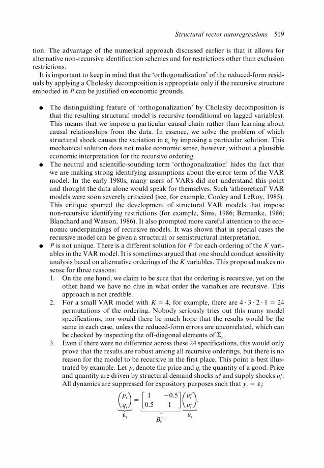
2. For a small VAR model with K 5 4, for example, there are 4 # 3 # 2 # 1 5 24 permutations of the ordering. Nobody seriously tries out this many model specifications, nor would there be much hope that the results would be the same in each case, unless the reduced- form errors are uncorrelated, which can be checked by inspecting the off- diagonal elements of Se.
3. Even if there were no difference across these 24 specifications, this would only prove that the results are robust among all recursive orderings, but there is no reason for the model to be recursive in the first place. This point is best illus-trated by example. Let pt denote the price and qt the quantity of a good. Price and quantity are driven by structural demand shocks ud
t and supply shocks ust .
All dynamics are suppressed for expository purposes such that yt 5 et:
apt
qtb 5 c 1 20.5
0.5 1d aud
t
ustb.
et B210
ut
HASHIMZADE 9780857931016 CHS. 22-23 (M3110).indd 519HASHIMZADE 9780857931016 CHS. 22-23 (M3110).indd 519 01/07/2013 10:3101/07/2013 10:31
520 Handbook of research methods and applications in empirical macroeconomics
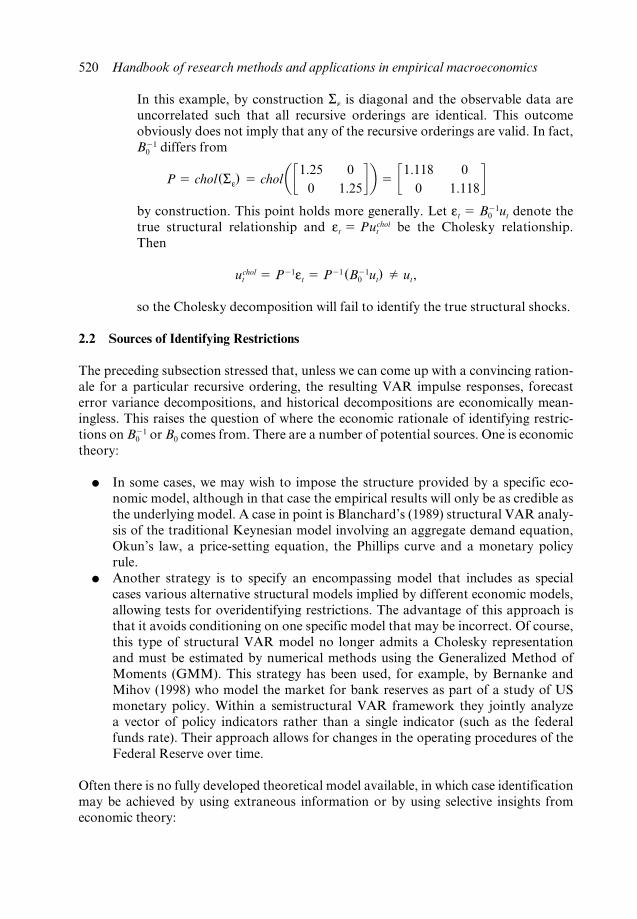
In this example, by construction Se is diagonal and the observable data are uncorrelated such that all recursive orderings are identical. This outcome obviously does not imply that any of the recursive orderings are valid. In fact, B21
0 differs from
P 5 chol(Se) 5 chol a c1.25 00 1.25
d b 5 c1.118 00 1.118
d by construction. This point holds more generally. Let et 5 B21
0 ut denote the true structural relationship and et 5 Puchol
t be the Cholesky relationship. Then
ucholt 5 P21et 5 P21 (B21
0 ut) 2 ut,
so the Cholesky decomposition will fail to identify the true structural shocks.
2.2 Sources of Identifying Restrictions
The preceding subsection stressed that, unless we can come up with a convincing ration-ale for a particular recursive ordering, the resulting VAR impulse responses, forecast error variance decompositions, and historical decompositions are economically mean-ingless. This raises the question of where the economic rationale of identifying restric-tions on B21
0 or B0 comes from. There are a number of potential sources. One is economic theory:
● In some cases, we may wish to impose the structure provided by a specific eco-nomic model, although in that case the empirical results will only be as credible as the underlying model. A case in point is Blanchard’s (1989) structural VAR analy-sis of the traditional Keynesian model involving an aggregate demand equation, Okun’s law, a price- setting equation, the Phillips curve and a monetary policy rule.
● Another strategy is to specify an encompassing model that includes as special cases various alternative structural models implied by different economic models, allowing tests for overidentifying restrictions. The advantage of this approach is that it avoids conditioning on one specific model that may be incorrect. Of course, this type of structural VAR model no longer admits a Cholesky representation and must be estimated by numerical methods using the Generalized Method of Moments (GMM). This strategy has been used, for example, by Bernanke and Mihov (1998) who model the market for bank reserves as part of a study of US monetary policy. Within a semistructural VAR framework they jointly analyze a vector of policy indicators rather than a single indicator (such as the federal funds rate). Their approach allows for changes in the operating procedures of the Federal Reserve over time.
Often there is no fully developed theoretical model available, in which case identification may be achieved by using extraneous information or by using selective insights from economic theory:
HASHIMZADE 9780857931016 CHS. 22-23 (M3110).indd 520HASHIMZADE 9780857931016 CHS. 22-23 (M3110).indd 520 01/07/2013 10:3101/07/2013 10:31
Structural vector autoregressions 521
● Information delays: information may not be available instantaneously because data are released only infrequently, allowing us to rule out instantaneous feed-back. This approach has been exploited in Inoue et al. (2009), for example.
● Physical constraints: for example, a firm may decide to invest, but it takes time for that decision to be made and for the new equipment to be installed, so measured physical investment responds with a delay.
● Institutional knowledge: for example, we may have information about the inabil-ity of suppliers to respond to demand shocks in the short run due to adjustment costs, which amounts to imposing a vertical slope on the supply curve (see, for example, Kilian, 2009). Similarly, Davis and Kilian (2011) exploit the fact that gasoline taxes (excluding ad valorem taxes) do not respond instantaneously to the state of the economy because lawmakers move at a slow pace. This feature of the data allows them to treat gasoline taxes as predetermined with respect to domes-tic macroeconomic aggregates. Moreover, given that consumers are effectively unable to store gasoline, anticipation of gasoline tax changes can be ignored in this setting.
● Assumptions about market structure: another common identifying assumption in empirical work is that there is no feedback from a small open economy to the rest of the world. This identifying assumption has been used, for example, to motivate treating US interest rates as contemporaneously exogenous with respect to the macroeconomic aggregates of small open economies such as Canada (see, for example, Cushman and Zha, 1997). This argument is not without limitations, however. Even if a small open economy is a price taker in world markets, both small and large economies may be driven by a common factor invalidating this exclusion restriction.
● Another possible source of identifying information is homogeneity restrictions on demand functions. For example, Galí (1992) imposes short- run homogeneity in the demand for money when assuming that the demand for real balances is not affected by contemporaneous changes in prices (given the nominal rate and output). This assumption amounts to assuming away costs of adjusting nominal money holdings. Similar homogeneity restrictions have also been used in Bernanke (1986).
● Extraneous parameter estimates: when impact responses (or their ratio) can be viewed as elasticities, it may be possible to impose values for those elasticities based on extraneous information from other studies. This approach has been used by Blanchard and Perotti (2002), for example. Similarly, Blanchard and Watson (1986) impose non- zero values for some structural parameters in B0 based on extraneous information. If the parameter value cannot be pinned down with any degree of reliability, yet another possibility is to explore a grid of possible structural parameters values, as in Abraham and Haltiwanger (1995). A similar approach has also been used in Kilian (2010) and Davis and Kilian (2011) in an effort to assess the robustness of their baseline results. In a different context, Todd (1990) interprets Sims’ (1980b) recursive VAR model of monetary policy in terms of alternative assumptions about the slopes of money demand and money supply curves.
● High- frequency data: in rare cases, it may be possible to test exclusion restrictions
HASHIMZADE 9780857931016 CHS. 22-23 (M3110).indd 521HASHIMZADE 9780857931016 CHS. 22-23 (M3110).indd 521 01/07/2013 10:3101/07/2013 10:31
522 Handbook of research methods and applications in empirical macroeconomics
more directly. For example, Kilian and Vega (2011) use daily data on US macro-economic news to formally test the identifying assumption of no feedback within the month from US macroeconomic aggregates to the price of oil. Their work lends credence to exclusion restrictions in monthly VAR models ruling out instan-taneous feedback from domestic macroeconomic aggregates to the price of oil.
It is fair to say that coming up with a set of credible short- run identifying restrictions is difficult. Whether a particular exclusion restriction is convincing, often depends on the data frequency, and in many cases there are not enough credible exclusion restrictions to achieve identification. This fact has stimulated interest in the alternative identification methods discussed in sections 3, 4 and 5.
2.3 Examples of Recursively Identified Models
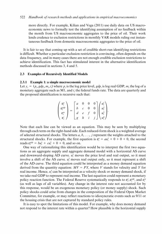
2.3.1 Example 1: a simple macroeconomic modelLet yt 5 (pt, gdpt, mt, it) where pt is the log price level, gdpt is log real GDP, mt the log of a monetary aggregate such as M1, and it the federal funds rate. The data are quarterly and the proposed identification is recursive such that:
± ept
egdpt
emt
eit
≤ 5 ≥ a 0 0 0b c 0 0d e f 0g h i j
¥ ± u1t
u2t
u3t
u4t
≤ .
Note that each line can be viewed as an equation. This may be seen by multiplying through each term on the right- hand side. Each reduced- form shock is a weighted average of selected structural shocks. The letters a, b, . . ., j represent the weights attached to the structural shocks. For example, the first equation is ep
t 5 au1t 1 0 1 0 1 0, the second
reads egdpt 5 bu1
t 1 cu2t 1 0 1 0, and so on.
One way of rationalizing this identification would be to interpret the first two equa-tions as an aggregate supply and aggregate demand model with a horizontal AS curve and downward- sloping AD curve. u1
t moves the price level and real output, so it must involve a shift of the AS curve. u2
t moves real output only, so it must represent a shift of the AD curve. The third equation could be interpreted as a money demand equation derived from the quantity equation: MV 5 PY, where V stands for velocity and Y for real income. Hence, u3
t can be interpreted as a velocity shock or money demand shock, if we take real GDP to represent real income. The last equation could represent a monetary policy reaction function. The Federal Reserve systematically responds to ep
t , egdpt , and em
t (as well as lags of all variables). Any change in the interest rate not accounted for by this response, would be an exogenous monetary policy (or money supply) shock. Such policy shocks could arise from changes in the composition of the Federal Open Market Committee, for example, or may reflect reactions to idiosyncratic events such as 9/11 or the housing crisis that are not captured by standard policy rules.
It is easy to spot the limitations of this model. For example, why does money demand not respond to the interest rate within a quarter? How plausible is the horizontal supply
HASHIMZADE 9780857931016 CHS. 22-23 (M3110).indd 522HASHIMZADE 9780857931016 CHS. 22-23 (M3110).indd 522 01/07/2013 10:3101/07/2013 10:31
Structural vector autoregressions 523
curve? These are the types of questions that one must ask when assessing the plausibil-ity of a structural VAR model. This example also illustrates that theory typically is not sufficient for identification, even if we are willing to condition on a particular theoreti-cal model. For example, if the AS curve were vertical, but the AD curve horizontal by assumption, the first two equations of the structural model above would have to be mod-ified. More generally, no recursive structure would be able to accommodate a theoretical model in which the AS and AD curves are neither horizontal nor vertical, but upward and downward sloping. This point highlights the difficulty of specifying fully structural models of the macroeconomy in recursive form and explains why such models have been largely abandoned.
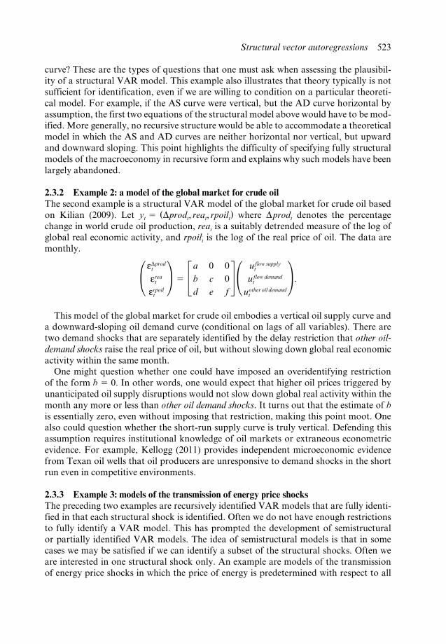
2.3.2 Example 2: a model of the global market for crude oilThe second example is a structural VAR model of the global market for crude oil based on Kilian (2009). Let yt 5 (Dprodt, reat, rpoilt) where Dprodt denotes the percentage change in world crude oil production, reat is a suitably detrended measure of the log of global real economic activity, and rpoilt is the log of the real price of oil. The data are monthly.
° eDprodt
ereat
erpoilt
¢ 5 £ a 0 0b c 0d e f
§ ° uflow supplyt
u flow demandt
uother oil demandt
¢ .
This model of the global market for crude oil embodies a vertical oil supply curve and a downward- sloping oil demand curve (conditional on lags of all variables). There are two demand shocks that are separately identified by the delay restriction that other oil- demand shocks raise the real price of oil, but without slowing down global real economic activity within the same month.
One might question whether one could have imposed an overidentifying restriction of the form b 5 0. In other words, one would expect that higher oil prices triggered by unanticipated oil supply disruptions would not slow down global real activity within the month any more or less than other oil demand shocks. It turns out that the estimate of b is essentially zero, even without imposing that restriction, making this point moot. One also could question whether the short- run supply curve is truly vertical. Defending this assumption requires institutional knowledge of oil markets or extraneous econometric evidence. For example, Kellogg (2011) provides independent microeconomic evidence from Texan oil wells that oil producers are unresponsive to demand shocks in the short run even in competitive environments.
2.3.3 Example 3: models of the transmission of energy price shocksThe preceding two examples are recursively identified VAR models that are fully identi-fied in that each structural shock is identified. Often we do not have enough restrictions to fully identify a VAR model. This has prompted the development of semistructural or partially identified VAR models. The idea of semistructural models is that in some cases we may be satisfied if we can identify a subset of the structural shocks. Often we are interested in one structural shock only. An example are models of the transmission of energy price shocks in which the price of energy is predetermined with respect to all
HASHIMZADE 9780857931016 CHS. 22-23 (M3110).indd 523HASHIMZADE 9780857931016 CHS. 22-23 (M3110).indd 523 01/07/2013 10:3101/07/2013 10:31
524 Handbook of research methods and applications in empirical macroeconomics
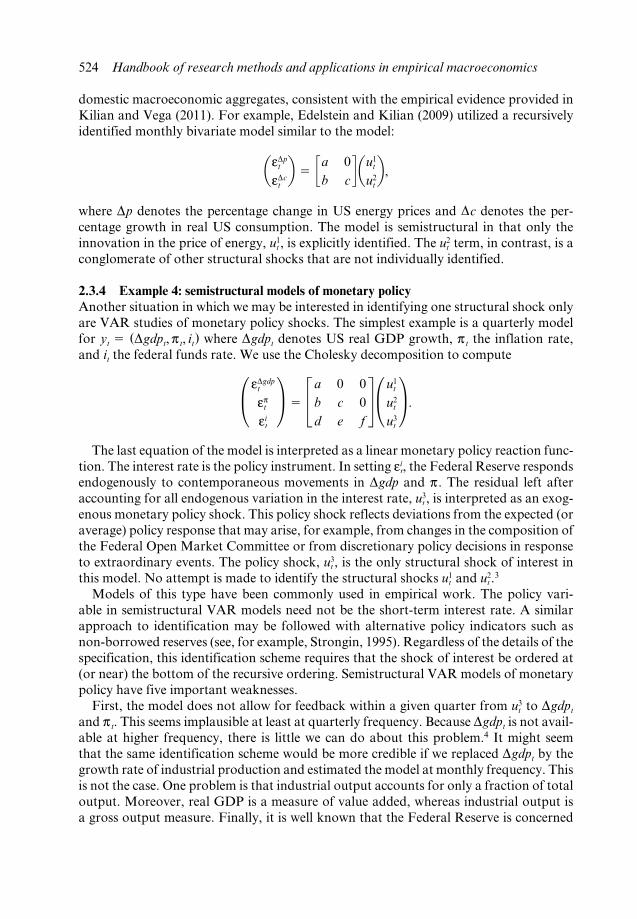
domestic macroeconomic aggregates, consistent with the empirical evidence provided in Kilian and Vega (2011). For example, Edelstein and Kilian (2009) utilized a recursively identified monthly bivariate model similar to the model:
aeDpt
eDctb 5 ca 0
b cd au1
t
u2tb,
where Dp denotes the percentage change in US energy prices and Dc denotes the per-centage growth in real US consumption. The model is semistructural in that only the innovation in the price of energy, u1
t , is explicitly identified. The u2t term, in contrast, is a
conglomerate of other structural shocks that are not individually identified.
2.3.4 Example 4: semistructural models of monetary policyAnother situation in which we may be interested in identifying one structural shock only are VAR studies of monetary policy shocks. The simplest example is a quarterly model for yt 5 (Dgdpt,pt, it) where Dgdpt denotes US real GDP growth, pt the inflation rate, and it the federal funds rate. We use the Cholesky decomposition to compute
° eDgdpt
ept
eit
¢ 5 £ a 0 0b c 0d e f
§ °u1t
u2t
u3t
¢ .
The last equation of the model is interpreted as a linear monetary policy reaction func-tion. The interest rate is the policy instrument. In setting ei
t, the Federal Reserve responds endogenously to contemporaneous movements in Dgdp and p. The residual left after accounting for all endogenous variation in the interest rate, u3
t , is interpreted as an exog-enous monetary policy shock. This policy shock reflects deviations from the expected (or average) policy response that may arise, for example, from changes in the composition of the Federal Open Market Committee or from discretionary policy decisions in response to extraordinary events. The policy shock, u3
t , is the only structural shock of interest in this model. No attempt is made to identify the structural shocks u1
t and u2t .3
Models of this type have been commonly used in empirical work. The policy vari-able in semistructural VAR models need not be the short- term interest rate. A similar approach to identification may be followed with alternative policy indicators such as non- borrowed reserves (see, for example, Strongin, 1995). Regardless of the details of the specification, this identification scheme requires that the shock of interest be ordered at (or near) the bottom of the recursive ordering. Semistructural VAR models of monetary policy have five important weaknesses.
First, the model does not allow for feedback within a given quarter from u3t to Dgdpt
and pt. This seems implausible at least at quarterly frequency. Because Dgdpt is not avail-able at higher frequency, there is little we can do about this problem.4 It might seem that the same identification scheme would be more credible if we replaced Dgdpt by the growth rate of industrial production and estimated the model at monthly frequency. This is not the case. One problem is that industrial output accounts for only a fraction of total output. Moreover, real GDP is a measure of value added, whereas industrial output is a gross output measure. Finally, it is well known that the Federal Reserve is concerned
HASHIMZADE 9780857931016 CHS. 22-23 (M3110).indd 524HASHIMZADE 9780857931016 CHS. 22-23 (M3110).indd 524 01/07/2013 10:3101/07/2013 10:31
Structural vector autoregressions 525
with broader measures of real activity, making a policy reaction function based on indus-trial production growth economically less plausible and hence less interesting. In this regard, a better measure of monthly US real activity would be the Chicago Fed’s monthly principal components index of US real activity (CFNAI). Yet another approach in the literature has been to interpolate quarterly real GDP data based on the fluctuations in monthly industrial production data and other monthly indicators. Such ad hoc methods not only suffer from the same deficiencies as the use of industrial production data, but they are likely to distort the structural impulse responses to be estimated.
Second, the Federal Reserve may respond systematically to more variables than just Dgdpt and pt. Examples are housing prices, stock prices, or industrial commodity prices. To the extent that we have omitted these variables from the model, we will obtain inconsistent estimates of d and e, and incorrect measures of the monetary policy shock u3
t . In essence, the problem is that the policy shocks must be exogenous to allow us to learn about the effects of monetary policy shocks. Thus, it is common to enrich the set of variables ordered above the interest rate relative to this simple benchmark model and estimate much larger VAR systems (see, for example, Bernanke and Blinder, 1992; Sims, 1992; Christiano et al., 1999).
Adding more variables, however, invites overfitting and undermines the credibility of the VAR estimates. Standard VAR models cannot handle more than half a dozen vari-ables, given typical sample sizes. One potential remedy of this problem is to work with factor augmented VAR (FAVAR) models, as in Bernanke and Boivin (2003), Bernanke et al. (2005), Stock and Watson (2005) or Forni et al. (2009). Alternatively, one can work with large- scale Bayesian VAR models in which the cross- sectional dimension K is allowed to be larger than the time dimension T, as in Banbura et al. (2010). These large- scale models are designed to incorporate a much richer information structure than conventional semistructural VAR models of monetary policy. FAVAR models and large- scale BVAR models have three distinct advantages over conventional small to medium sized VAR models. First, they allow for the fact that central bankers form expectations about domestic real activity and inflation based on hundreds of economic and financial time series rather than a handful of time series. Second, they allow for the fact that economic concepts such as domestic economic activity and inflation may not be well represented by a single observable time series. Third, they allow the user to con-struct the responses of many variables not included in conventional VAR models. There is evidence that allowing for richer information sets in specifying VAR models improves the plausibility of the estimated responses. It may mitigate the price puzzle, for example.5
Third, the identification of the VAR model hinges on the monetary policy reaction function being stable over time. To the extent that policymakers have at times changed the weights attached to their inflation and output objectives or the policy instrument, it becomes essential to split the sample in estimating the VAR model. The resulting shorter sample in turn makes it more difficult to include many variables in the model due to the lack of degrees of freedom. It also complicates statistical inference.
Fourth, the VAR model is linear. It does not allow for a lower bound on the interest rate, for example, making this model unsuitable for studying the quantitative easing of the Federal Reserve Board in recent years.
Fifth, most VAR models of monetary policy ignore the real- time nature of the policy decision problem. Not all data relevant to policymakers are available without delay and
HASHIMZADE 9780857931016 CHS. 22-23 (M3110).indd 525HASHIMZADE 9780857931016 CHS. 22-23 (M3110).indd 525 01/07/2013 10:3101/07/2013 10:31
526 Handbook of research methods and applications in empirical macroeconomics
when data become available, they tend to be preliminary and subject to further revisions. To the extent that monetary policy shocks are defined as the residual of the policy reac-tion function, a misspecification of the policymaker’s information set will cause biases in the estimated policy shocks. Bernanke and Boivin (2003) is an example of a study that explores the role of real- time data limitations in semistructural VAR models. Their con-clusion is that 2 at least for their sample period 2 the distinction between real- time data and ex- post revised data is of limited importance.
Finally, it is useful to reiterate that the thought experiment contemplated in structural VAR models is an unanticipated monetary policy shock within an existing monetary policy rule. This exercise is distinct from that of changing the monetary policy rule (as happened in 1979 under Paul Volcker or in 2008 following the quantitative easing of the Federal Reserve Board). The latter question is of independent interest, but much harder to answer. The role of systematic monetary policy has been stressed in Leeper et al. (1996) and Bernanke et al. (1997), for example. Econometric evaluations of the role of systematic monetary policy, however, remain controversial and easily run afoul of the Lucas critique (see, for example, Kilian and Lewis (2011) and the references therein).
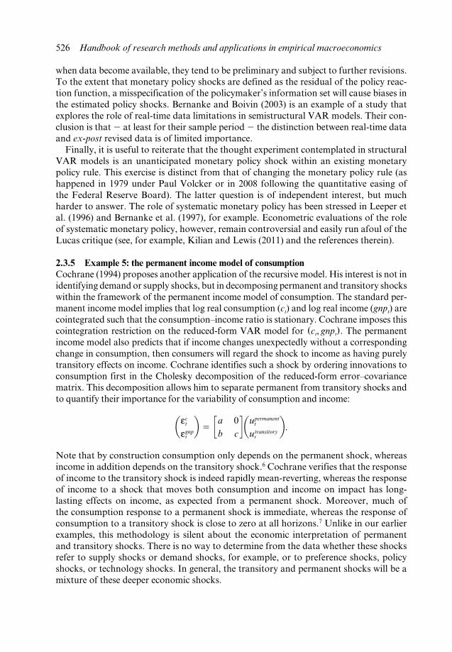
2.3.5 Example 5: the permanent income model of consumptionCochrane (1994) proposes another application of the recursive model. His interest is not in identifying demand or supply shocks, but in decomposing permanent and transitory shocks within the framework of the permanent income model of consumption. The standard per-manent income model implies that log real consumption (ct) and log real income (gnpt) are cointegrated such that the consumption–income ratio is stationary. Cochrane imposes this cointegration restriction on the reduced- form VAR model for (ct, gnpt). The permanent income model also predicts that if income changes unexpectedly without a corresponding change in consumption, then consumers will regard the shock to income as having purely transitory effects on income. Cochrane identifies such a shock by ordering innovations to consumption first in the Cholesky decomposition of the reduced- form error–covariance matrix. This decomposition allows him to separate permanent from transitory shocks and to quantify their importance for the variability of consumption and income:
aect
egnptb 5 ca 0
b cd aupermanent
t
utransitoryt
b.
Note that by construction consumption only depends on the permanent shock, whereas income in addition depends on the transitory shock.6 Cochrane verifies that the response of income to the transitory shock is indeed rapidly mean- reverting, whereas the response of income to a shock that moves both consumption and income on impact has long- lasting effects on income, as expected from a permanent shock. Moreover, much of the consumption response to a permanent shock is immediate, whereas the response of consumption to a transitory shock is close to zero at all horizons.7 Unlike in our earlier examples, this methodology is silent about the economic interpretation of permanent and transitory shocks. There is no way to determine from the data whether these shocks refer to supply shocks or demand shocks, for example, or to preference shocks, policy shocks, or technology shocks. In general, the transitory and permanent shocks will be a mixture of these deeper economic shocks.
HASHIMZADE 9780857931016 CHS. 22-23 (M3110).indd 526HASHIMZADE 9780857931016 CHS. 22-23 (M3110).indd 526 01/07/2013 10:3101/07/2013 10:31
Structural vector autoregressions 527
2.4 Examples of Non- recursively Identified Models
Not all structural VAR models have a recursive structure. Increasing skepticism toward atheoretical recursively identified models in the mid- 1980s stimulated a series of studies proposing explicitly structural models identified by non- recursive short- run restrictions (see, for example, Bernanke, 1986; Sims, 1986; Blanchard and Watson, 1986). As in the recursive model, the identifying restrictions on B0 or B21
0 generate moment condi-tions that can be used to estimate the unknown coefficients in B0. Efficient estimation of B0 in these models can be cast in a GMM framework in which, in addition to the predetermined variables in the reduced form, the estimated structural errors are used as instruments in the equations with which the structural errors are assumed uncorrelated. In general, solving the moment conditions for the unknown structural parameters will require iteration, but in some cases the GMM estimator can be constructed using tra-ditional instrumental- variable techniques (see, for example, Watson, 1994; Pagan and Robertson, 1998). An alternative commonly used approach is to model the error distri-bution as Gaussian and to estimate the structural model by full information maximum likelihood methods. This approach involves the maximization.of the concentrated likeli-hood with respect to the structural model parameters subject to the identifying restric-tions (see, for example, Lütkepohl, 2005).
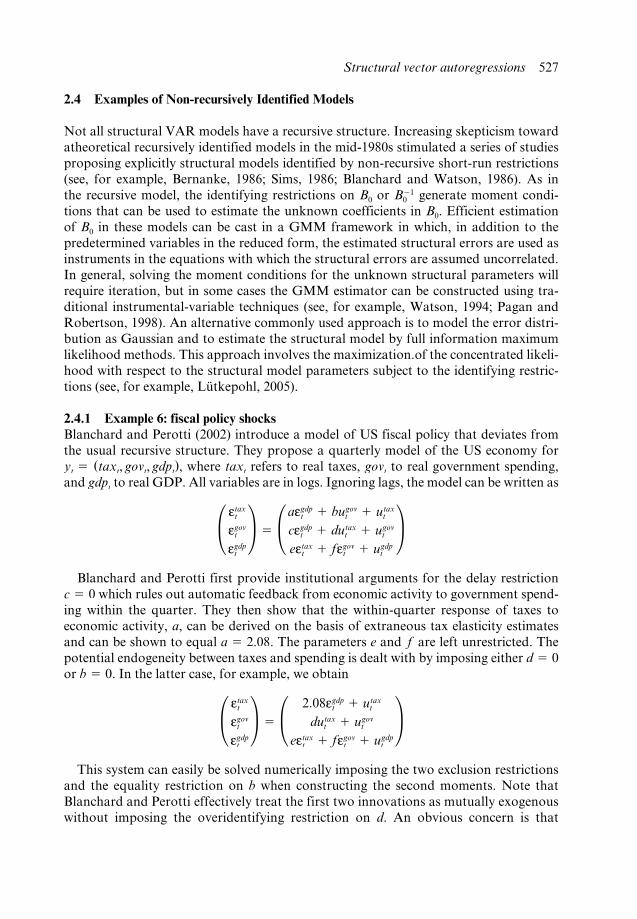
2.4.1 Example 6: fiscal policy shocksBlanchard and Perotti (2002) introduce a model of US fiscal policy that deviates from the usual recursive structure. They propose a quarterly model of the US economy for yt 5 (taxt, govt, gdpt), where taxt refers to real taxes, govt to real government spending, and gdpt to real GDP. All variables are in logs. Ignoring lags, the model can be written as
° etaxt
egovt
egdpt
¢ 5 °aegdpt 1 bugov
t 1 utaxt
cegdpt 1 dutax
t 1 ugovt
eetaxt 1 fegov
t 1 ugdpt
¢Blanchard and Perotti first provide institutional arguments for the delay restriction
c 5 0 which rules out automatic feedback from economic activity to government spend-ing within the quarter. They then show that the within- quarter response of taxes to economic activity, a, can be derived on the basis of extraneous tax elasticity estimates and can be shown to equal a 5 2.08. The parameters e and f are left unrestricted. The potential endogeneity between taxes and spending is dealt with by imposing either d 5 0 or b 5 0. In the latter case, for example, we obtain
° etaxt
egovt
egdpt
¢ 5 ° 2.08egdpt 1 utax
t
dutaxt 1 ugov
t
eetaxt 1 fegov
t 1 ugdpt
¢This system can easily be solved numerically imposing the two exclusion restrictions
and the equality restriction on b when constructing the second moments. Note that Blanchard and Perotti effectively treat the first two innovations as mutually exogenous without imposing the overidentifying restriction on d. An obvious concern is that
HASHIMZADE 9780857931016 CHS. 22-23 (M3110).indd 527HASHIMZADE 9780857931016 CHS. 22-23 (M3110).indd 527 01/07/2013 10:3101/07/2013 10:31
528 Handbook of research methods and applications in empirical macroeconomics
the model does not allow for the anticipation of fiscal shocks. Blanchard and Perotti discuss how this concern may be addressed by changing the timing assumptions and adding further identifying restrictions, if we are willing to postulate a specific form of foresight. Another concern is that the model does not condition on the debt structure (see, for example, Chung and Leeper, 2007). Allowing the debt structure to matter would result in a non- linear dynamic model not contained within the class of VAR models.
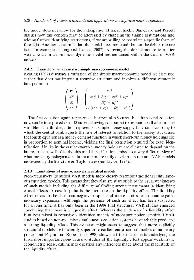
2.4.2 Example 7: an alternative simple macroeconomic modelKeating (1992) discusses a variation of the simple macroeconomic model we discussed earlier that does not impose a recursive structure and involves a different economic interpretation:
± ept
egdpt
eit
emt
≤ 5 ± uASt
aept 1 bei
t 1 cemt 1 uIS
t
demt 1 uMS
t
e(egdpt 1 ep
t ) 1 feit 1 uMD
t
≤The first equation again represents a horizontal AS curve, but the second equation
now can be interpreted as an IS curve, allowing real output to respond to all other model variables. The third equation represents a simple money supply function, according to which the central bank adjusts the rate of interest in relation to the money stock, and the fourth equation is a money demand function in which short- run money holdings rise in proportion to nominal income, yielding the final restriction required for exact iden-tification. Unlike in the earlier example, money holdings are allowed to depend on the interest rate as well. Clearly, this model specification embodies a very different view of what monetary policymakers do than more recently developed structural VAR models motivated by the literature on Taylor rules (see Taylor, 1993).
2.4.3 Limitations of non- recursively identified modelsNon- recursively identified VAR models more closely resemble traditional simultane-ous equation models. This means that they also are susceptible to the usual weaknesses of such models including the difficulty of finding strong instruments in identifying causal effects. A case in point is the literature on the liquidity effect. The liquidity effect refers to the short- run negative response of interest rates to an unanticipated monetary expansion. Although the presence of such an effect has been suspected for a long time, it has only been in the 1990s that structural VAR studies emerged concluding that there is a liquidity effect. Whereas the evidence of a liquidity effect is at best mixed in recursively identified models of monetary policy, empirical VAR studies based on non- recursive simultaneous equation systems have reliably produced a strong liquidity effect. This evidence might seem to suggest that more explicitly structural models are inherently superior to earlier semistructural models of monetary policy, but Pagan and Robertson (1998) show that the instruments underlying the three most important non- recursive studies of the liquidity effect appear weak in the econometric sense, calling into question any inferences made about the magnitude of the liquidity effect.
HASHIMZADE 9780857931016 CHS. 22-23 (M3110).indd 528HASHIMZADE 9780857931016 CHS. 22-23 (M3110).indd 528 01/07/2013 10:3101/07/2013 10:31
Structural vector autoregressions 529
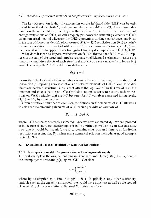
3 IDENTIFICATION BY LONG- RUN RESTRICTIONS
One alternative idea has been to impose restrictions on the long- run response of vari-ables to shocks. In the presence of unit roots in some variables but not in others, this may allow us to identify at least some shocks. The promise of this alternative approach to identification is that it will allow us to dispense with the controversy about what the right short- run restrictions are and to focus on long- run properties of models that most economists can more easily agree on. For example, it has been observed that most econo-mists agree that demand shocks such as monetary policy shocks are neutral in the long run, whereas productivity shocks are not. This idea was first introduced in the context of a bivariate model in Blanchard and Quah (1989).
Consider the structural VAR representation B(L)yt 5 ut and the corresponding structural vector moving average (VMA) representation yt 5 B(L)21ut 5 Q(L)ut. Also consider the reduced- form VAR model A(L)yt 5 et and the corresponding reduced- form VMA representation yt 5 A(L)21et 5 F(L)et.. By definition
et 5 B210 ut
Se 5 B210 B21r0
where we imposed Su 5 IK. Recall that
A(L) 5 B210 B(L)
B210 5 A(L)B(L)21
so for L 5 1
B210 5 A(1)B(1)21
and hence
Se 5 B210 B21r0
5 [A(1)B(1)21 ] [A(1)B(1)21 ]r
[B(1)21 ]rA (1)r
Premultiply both sides by A(1)21 and post- multiply both sides by (A(1)21)r 5 [A(1)r ]21:
A(1)21Se (A(1)21)r 5 A(1)21A(1)B(1)21 [B(1)21 ]rA(1)r [A(1)r ]21
A(1)21Se (A(1)21)r 5 [B(1)21 ] [B(1)21 ]r
F(1)SeF(1)r 5 Q(1)Q(1)r
vec(F(1)SeF(1)r) 5 vec(Q(1)Q(1)r)
HASHIMZADE 9780857931016 CHS. 22-23 (M3110).indd 529HASHIMZADE 9780857931016 CHS. 22-23 (M3110).indd 529 01/07/2013 10:3101/07/2013 10:31
530 Handbook of research methods and applications in empirical macroeconomics
The key observation is that the expression on the left- hand side (LHS) can be esti-mated from the data. Both Se and the cumulative sum F(1) 5 A(1)21 are observable based on the reduced- form model, given that A(1) ; I 2 A1 2 . . . 2 Ap, so if we put enough restrictions on Q(1) , we can uniquely pin down the remaining elements of Q(1) using numerical methods. Because the LHS represents a variance–covariance matrix, as in the case of short- run identification, we need K(K 2 1) /2 restrictions on Q(1) to satisfy the order condition for exact identification. If the exclusion restrictions on Q(1) are recursive, it suffices to apply a lower triangular Cholesky decomposition to F(1)SeF(1)r.
What does it mean to impose restrictions on Q(1)? Observe that Q(1) 5 B(1)21 rep-resents the sum of the structural impulse response coefficients. Its elements measure the long- run cumulative effects of each structural shock j on each variable i, so, for an I(1) variable entering the VAR model in log differences,
Qij(1) 5 0
means that the log- level of this variable i is not affected in the long run by structural innovation j. Imposing zero restrictions on selected elements of Q(1) allows us to dif-ferentiate between structural shocks that affect the log- level of an I(1) variable in the long run and shocks that do not. Clearly, it does not make sense to put any such restric-tions on VAR variables that are I(0) because, for I(0) variables expressed in log- levels, Qij(1) 2 0 4j by construction.
Given a sufficient number of exclusion restrictions on the elements of Q(1) allows us to solve for the remaining elements of Q(1) , which provides an estimate of
B210 5 A(1)Q(1) ,
where A(1) can be consistently estimated. Once we have estimated B210 , we can proceed
as in the case of short- run identifying restrictions. Although we do not consider this case, note that it would be straightforward to combine short- run and long- run identifying restrictions in estimating B21
0 , when using numerical solution methods. A good example is Galí (1992).
3.1 Examples of Models Identified by Long- run Restrictions
3.1.1 Example 8: a model of aggregate demand and aggregate supplyThe first example is the original analysis in Blanchard and Quah (1989). Let urt denote the unemployment rate and gdpt log real GDP. Consider
yt 5 aDgdpt
urtb
where by assumption yt , I(0) , but gdpt , I(1) . In principle, any other stationary variable such as the capacity utilization rate would have done just as well as the second element of yt. After postulating a diagonal Su matrix, we obtain:
B(1)yt 5 ut
HASHIMZADE 9780857931016 CHS. 22-23 (M3110).indd 530HASHIMZADE 9780857931016 CHS. 22-23 (M3110).indd 530 01/07/2013 10:3101/07/2013 10:31
Structural vector autoregressions 531
c 1 02b1 1
d aDgdpt
urtb 5 auAS
t
uADtb
aDgdpt
urtb 5 c 1 0
2a1 1d 21auAS
t
uADtb
yt 5 Q(1)ut
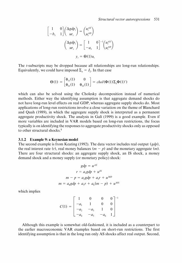
The t- subscripts may be dropped because all relationships are long- run relationships. Equivalently, we could have imposed Su 5 I2. In that case
Q(1) 5 cq11 (1) 0q21 (1) q22 (1) d 5 chol (F(1)SeF(1)r)
which can also be solved using the Cholesky decomposition instead of numerical methods. Either way the identifying assumption is that aggregate demand shocks do not have long- run level effects on real GDP, whereas aggregate supply shocks do. Most applications of long- run restrictions involve a close variation on the theme of Blanchard and Quah (1989), in which the aggregate supply shock is interpreted as a permanent aggregate productivity shock. The analysis in Galí (1999) is a good example. Even if more variables are included in VAR models based on long- run restrictions, the focus typically is on identifying the responses to aggregate productivity shocks only as opposed to other structural shocks.8
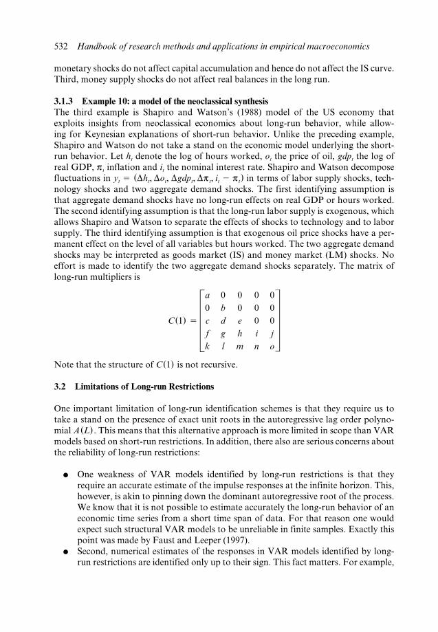
3.1.2 Example 9: a Keynesian modelThe second example is from Keating (1992). The data vector includes real output (gdp), the real interest rate (r), real money balances (m 2 p) and the monetary aggregate (m). There are four structural shocks: an aggregate supply shock, an IS shock, a money demand shock and a money supply (or monetary policy) shock:
gdp 5 uAS
r 5 a1gdp 1 uIS
m 2 p 5 a2gdp 1 a3r 1 uMD
m 5 a4gdp 1 a5r 1 a6 (m 2 p) 1 uMS
which implies
C(1) 5 ≥ 1 0 0 02a1 1 0 02a2 2a3 1 02a4 2a5 2a6 1
¥21
Although this example is somewhat old- fashioned, it is included as a counterpart to the earlier macroeconomic VAR examples based on short- run restrictions. The first identifying assumption is that in the long run only AS shocks affect real output. Second,
HASHIMZADE 9780857931016 CHS. 22-23 (M3110).indd 531HASHIMZADE 9780857931016 CHS. 22-23 (M3110).indd 531 01/07/2013 10:3101/07/2013 10:31
532 Handbook of research methods and applications in empirical macroeconomics
monetary shocks do not affect capital accumulation and hence do not affect the IS curve. Third, money supply shocks do not affect real balances in the long run.
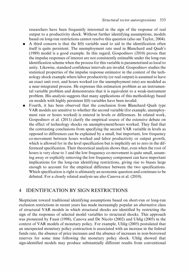
3.1.3 Example 10: a model of the neoclassical synthesisThe third example is Shapiro and Watson’s (1988) model of the US economy that exploits insights from neoclassical economics about long- run behavior, while allow-ing for Keynesian explanations of short- run behavior. Unlike the preceding example, Shapiro and Watson do not take a stand on the economic model underlying the short- run behavior. Let ht denote the log of hours worked, ot the price of oil, gdpt the log of real GDP, pt inflation and it the nominal interest rate. Shapiro and Watson decompose fluctuations in yt 5 (Dht, Dot, Dgdpt, Dpt, it 2 pt) in terms of labor supply shocks, tech-nology shocks and two aggregate demand shocks. The first identifying assumption is that aggregate demand shocks have no long- run effects on real GDP or hours worked. The second identifying assumption is that the long- run labor supply is exogenous, which allows Shapiro and Watson to separate the effects of shocks to technology and to labor supply. The third identifying assumption is that exogenous oil price shocks have a per-manent effect on the level of all variables but hours worked. The two aggregate demand shocks may be interpreted as goods market (IS) and money market (LM) shocks. No effort is made to identify the two aggregate demand shocks separately. The matrix of long- run multipliers is
C(1) 5 Ea 0 0 0 00 b 0 0 0c d e 0 0f g h i jk l m n o
UNote that the structure of C(1) is not recursive.
3.2 Limitations of Long- run Restrictions
One important limitation of long- run identification schemes is that they require us to take a stand on the presence of exact unit roots in the autoregressive lag order polyno-mial A(L) . This means that this alternative approach is more limited in scope than VAR models based on short- run restrictions. In addition, there also are serious concerns about the reliability of long- run restrictions:
● One weakness of VAR models identified by long- run restrictions is that they require an accurate estimate of the impulse responses at the infinite horizon. This, however, is akin to pinning down the dominant autoregressive root of the process. We know that it is not possible to estimate accurately the long- run behavior of an economic time series from a short time span of data. For that reason one would expect such structural VAR models to be unreliable in finite samples. Exactly this point was made by Faust and Leeper (1997).
● Second, numerical estimates of the responses in VAR models identified by long- run restrictions are identified only up to their sign. This fact matters. For example,
HASHIMZADE 9780857931016 CHS. 22-23 (M3110).indd 532HASHIMZADE 9780857931016 CHS. 22-23 (M3110).indd 532 01/07/2013 10:3101/07/2013 10:31
Structural vector autoregressions 533
researchers have been frequently interested in the sign of the response of real output to a productivity shock. Without further identifying assumptions, models based on long- run restrictions cannot resolve this question (also see Taylor, 2004).
● A third concern is that the I(0) variable used to aid in the identification often itself is quite persistent. The unemployment rate used in Blanchard and Quah’s (1989) model is a good example. In this regard, Gospodinov (2010) proves that the impulse responses of interest are not consistently estimable under the long- run identification scheme when the process for this variable is parameterized as local to unity. Likewise, standard confidence intervals are invalid. Gospodinov studies the statistical properties of the impulse response estimator in the context of the tech-nology shock example where labor productivity (or real output) is assumed to have an exact unit root, and hours worked (or the unemployment rate) are modeled as a near- integrated process. He expresses this estimation problem as an instrumen-tal variable problem and demonstrates that it is equivalent to a weak- instrument problem. His analysis suggests that many applications of this methodology based on models with highly persistent I(0) variables have been invalid.
● Fourth, it has been observed that the conclusion from Blanchard–Quah type VAR models are sensitive to whether the second variable (for example, unemploy-ment rate or hours worked) is entered in levels or differences. In related work, Gospodinov et al. (2011) clarify the empirical source of the extensive debate on the effect of technology shocks on unemployment/hours worked. They find that the contrasting conclusions from specifying the second VAR variable in levels as opposed to differences can be explained by a small, but important, low frequency co- movement between hours worked and labor productivity or output growth, which is allowed for in the level specification but is implicitly set to zero in the dif-ferenced specification. Their theoretical analysis shows that, even when the root of hours is very close to 1 and the low frequency co- movement is quite small, assum-ing away or explicitly removing the low frequency component can have important implications for the long- run identifying restrictions, giving rise to biases large enough to account for the empirical difference between the two specifications. Which specification is right is ultimately an economic question and continues to be debated. For a closely related analysis see also Canova et al. (2010).
4 IDENTIFICATION BY SIGN RESTRICTIONS
Skepticism toward traditional identifying assumptions based on short- run or long- run exclusion restrictions in recent years has made increasingly popular an alternative class of structural VAR models in which structural shocks are identified by restricting the sign of the responses of selected model variables to structural shocks. This approach was pioneered by Faust (1998), Canova and De Nicolo (2002) and Uhlig (2005) in the context of VAR models of monetary policy. For example, Uhlig (2005) postulated that an unexpected monetary policy contraction is associated with an increase in the federal funds rate, the absence of price increases and the absence of increases in non- borrowed reserves for some time following the monetary policy shock. Uhlig showed that sign- identified models may produce substantially different results from conventional
HASHIMZADE 9780857931016 CHS. 22-23 (M3110).indd 533HASHIMZADE 9780857931016 CHS. 22-23 (M3110).indd 533 01/07/2013 10:3101/07/2013 10:31
534 Handbook of research methods and applications in empirical macroeconomics
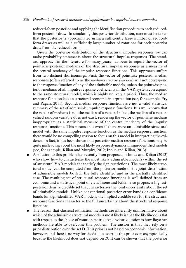
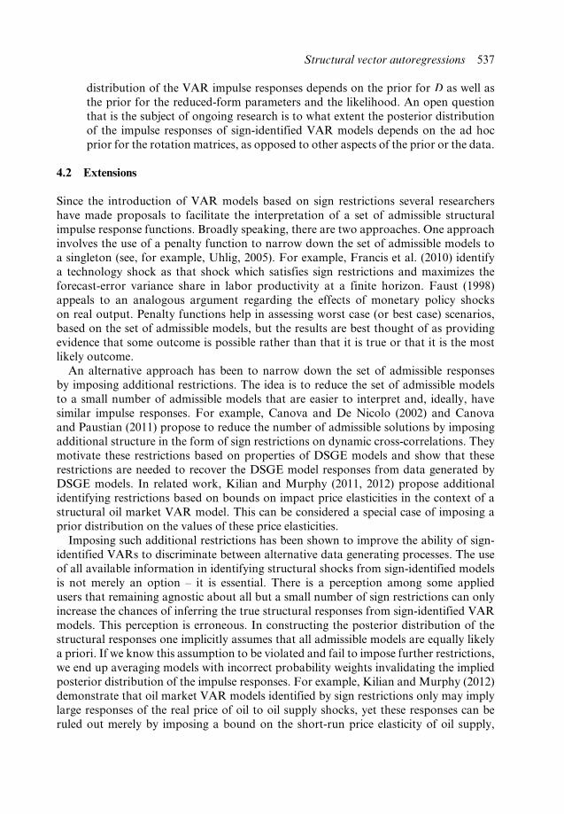
structural VAR models. Sign- identified VAR models have become increasingly popular in other areas as well and are now part of the mainstream of empirical macroeconomics. They have been used to study fiscal shocks (for example, Canova and Pappa, 2007; Mountford and Uhlig, 2009; Pappa, 2009), technology shocks (for example, Dedola and Neri, 2007), and various other shocks in open economies (for example, Canova and De Nicolo, 2002; Scholl and Uhlig, 2008), in oil markets (for example, Baumeister and Peersman, 2012; Kilian and Murphy, 2012, 2013), and in labor markets (for example, Fujita, 2011).
Identification in sign- identified models requires that each identified shock is associ-ated with a unique sign pattern. Sign restrictions may be static, in which case we simply restrict the sign of the coefficients in B21
0 . Unlike traditional exclusion restrictions, such sign restrictions can often be motivated directly from economic theory. In addition, one may restrict the sign of responses at longer horizons, although the theoretical rationale of such restrictions is usually weaker. There is a misperception among many users that these models are more general and hence more credible than VAR models based on exclusion restrictions. This is not the case. Note that sign- identified models by construc-tion are more restrictive than standard VAR models in some dimensions and less restric-tive in others. They do not nest models based on exclusion restrictions.
For a given set of sign restrictions, we proceed as follows. Consider the reduced- form VAR model A(L)yt 5 et, where yt is the K- dimensional vector of variables, A(L) is a finite- order autoregressive lag polynomial, and et is the vector of white noise reduced- form innovations with variance–covariance matrix Se. Let ut denote the corresponding structural VAR model innovations. The construction of structural impulse response functions requires an estimate of the K 3 K matrix B21
0 in et 5 B210 ut.
Let P denote the lower triangular Cholesky decomposition that satisfies Se 5 PPr. Then B21
0 5 PD also satisfies Se 5 B210 B21
0 r for any orthogonal K 3 K matrix D. Unlike P, PD will in general be non- recursive. One can examine a wide range of possible solu-tions B21
0 by repeatedly drawing at random from the set D of orthogonal matrices D. Following Rubio- Ramirez et al. (2010) one constructs the set of admissible models by drawing from the set D and discarding candidate solutions for B21
0 that do not satisfy a set of a priori sign restrictions on the implied impulse responses functions.
The procedure consists of the following steps:
1. Draw a K 3 K matrix L of NID(0, 1) random variables. Derive the QR decomposi-tion of L such that L 5 Q # R and QQ r 5 IK.
2. Let D 5 Q r. Compute impulse responses using the orthogonalization B210 5 PD. If
all implied impulse response functions satisfy the identifying restrictions, retain D. Otherwise discard D.
3. Repeat the first two steps a large number of times, recording each D that satisfies the restrictions (and the corresponding impulse response functions).
The resulting set B210 in conjunction with the reduced- form estimates characterizes the
set of admissible structural VAR models.The fraction of the initial candidate models that satisfy the identifying restriction may
be viewed as an indicator of how informative the identifying restrictions are about the structural parameters. Note that a small fraction of admissible models is not an indica-
HASHIMZADE 9780857931016 CHS. 22-23 (M3110).indd 534HASHIMZADE 9780857931016 CHS. 22-23 (M3110).indd 534 01/07/2013 10:3101/07/2013 10:31

Structural vector autoregressions 535
tion of how well the identifying restrictions fit the data. There is no way of evaluating the validity of identifying restrictions based on the reduced form. All candidate models by construction fit the data equally well because they are constructed from the same reduced- form model.
4.1 Interpretation
A fundamental problem in interpreting VAR models identified based on sign restric-tions is that there is not a unique point estimate of the structural impulse response functions. Unlike conventional structural VAR models based on short- run restrictions, sign- identified VAR models are only set identified. This problem arises because sign restrictions represent inequality restrictions. The cost of remaining agnostic about the precise values of the structural model parameters is that the data are potentially consist-ent with a wide range of structural models that are all admissible in that they satisfy the identifying restrictions. Without further assumptions there is no way of knowing which of these models is most likely. A likely outcome in practice is that the structural impulse responses implied by the admissible models will disagree on the substantive economic questions of interest.
● One early approach to this problem, exemplified by Faust (1998), has been to focus on the admissible model that is most favorable to the hypothesis of interest. This allows us to establish the extent to which this hypothesis could potentially explain the data. It may also help us to rule out a hypothesized explanation, if none of the admissible models supports this hypothesis. The problem is that this approach is not informative about whether any one of the admissible models is a more likely explanation of the data than some other model. There are examples in which the admissible structural models are sufficiently similar to allow unambiguous answers to the question of economic interest (see, for example, Kilian and Murphy, 2012, 2013). Typically, however, the set of admissible models will be equally consistent with competing economic hypotheses.
● The standard procedure for characterizing the set of admissible models outlined above conditions on a given estimate of the reduced- form VAR model and does not account for estimation uncertainty. A method of constructing classical confi-dence intervals for sign- identified VAR impulse responses has recently been devel-oped by Moon et al. (2009). Unlike in structural VAR models based on exclusion restrictions, the asymptotic distribution of the structural impulse responses is non- standard and the construction of these non- standard confidence intervals is computationally costly. Moreover, these intervals are not informative about the shape of the impulse response functions in that a given confidence set is consistent with a wide range of different shapes. This fact makes it difficult to interpret the results from an economic point of view.
● The most common approach in the literature has been to rely on Bayesian methods of inference. Under the assumption of a conventional Gaussian- inverse Wishart prior on the reduced- form parameters and a prior on the rotation matrices con-ditional on a given reduced- form model estimate, one can construct the posterior distribution of the impulse responses by simulating posterior draws from the
HASHIMZADE 9780857931016 CHS. 22-23 (M3110).indd 535HASHIMZADE 9780857931016 CHS. 22-23 (M3110).indd 535 01/07/2013 10:3101/07/2013 10:31
536 Handbook of research methods and applications in empirical macroeconomics
reduced- form posterior and applying the identification procedure to each reduced- form posterior draw. In simulating this posterior distribution, care must be taken that the posterior is approximated using a sufficiently large number of reduced- form draws as well as a sufficiently large number of rotations for each posterior draw from the reduced form.
Given the posterior distribution of the structural impulse responses we can make probability statements about the structural impulse responses. The stand-ard approach in the literature for many years has been to report the vector of pointwise posterior medians of the structural impulse responses as a measure of the central tendency of the impulse response functions. This approach suffers from two distinct shortcomings. First, the vector of pointwise posterior median responses (often referred to as the median response function) will not correspond to the response function of any of the admissible models, unless the pointwise pos-terior medians of all impulse response coefficients in the VAR system correspond to the same structural model, which is highly unlikely a priori. Thus, the median response function lacks a structural economic interpretation (see, for example, Fry and Pagan, 2011). Second, median response functions are not a valid statistical summary of the set of admissible impulse response functions. It is well known that the vector of medians is not the median of a vector. In fact, the median of a vector- valued random variable does not exist, rendering the vector of pointwise medians inappropriate as a statistical measure of the central tendency of the impulse response functions. This means that even if there were an admissible structural model with the same impulse response function as the median response function, there would be no compelling reason to focus on this model in interpreting the evi-dence. In fact, it has been shown that posterior median response functions may be quite misleading about the most likely response dynamics in sign- identified models (see, for example, Kilian and Murphy, 2012; Inoue and Kilian, 2013).
● A solution to this problem has recently been proposed in Inoue and Kilian (2013) who show how to characterize the most likely admissible model(s) within the set of structural VAR models that satisfy the sign restrictions. The most likely struc-tural model can be computed from the posterior mode of the joint distribution of admissible models both in the fully identified and in the partially identified case. The resulting set of structural response functions is well defined from an economic and a statistical point of view. Inoue and Kilian also propose a highest- posterior density credible set that characterizes the joint uncertainty about the set of admissible models. Unlike conventional posterior error bands or confidence bands for sign- identified VAR models, the implied credible sets for the structural response functions characterize the full uncertainty about the structural response functions.
● The reason that classical estimation methods are inherently uninformative about which of the admissible structural models is most likely is that the likelihood is flat with respect to the choice of rotation matrix. An obvious question is how Bayesian methods are able to overcome this problem. The answer is that they rely on a prior distribution over the set D. This prior is not based on economic information, however, and there is no way for the data to overrule this prior even asymptotically because the likelihood does not depend on D. It can be shown that the posterior
HASHIMZADE 9780857931016 CHS. 22-23 (M3110).indd 536HASHIMZADE 9780857931016 CHS. 22-23 (M3110).indd 536 01/07/2013 10:3101/07/2013 10:31
Structural vector autoregressions 537
distribution of the VAR impulse responses depends on the prior for D as well as the prior for the reduced- form parameters and the likelihood. An open question that is the subject of ongoing research is to what extent the posterior distribution of the impulse responses of sign- identified VAR models depends on the ad hoc prior for the rotation matrices, as opposed to other aspects of the prior or the data.
4.2 Extensions
Since the introduction of VAR models based on sign restrictions several researchers have made proposals to facilitate the interpretation of a set of admissible structural impulse response functions. Broadly speaking, there are two approaches. One approach involves the use of a penalty function to narrow down the set of admissible models to a singleton (see, for example, Uhlig, 2005). For example, Francis et al. (2010) identify a technology shock as that shock which satisfies sign restrictions and maximizes the forecast- error variance share in labor productivity at a finite horizon. Faust (1998) appeals to an analogous argument regarding the effects of monetary policy shocks on real output. Penalty functions help in assessing worst case (or best case) scenarios, based on the set of admissible models, but the results are best thought of as providing evidence that some outcome is possible rather than that it is true or that it is the most likely outcome.
An alternative approach has been to narrow down the set of admissible responses by imposing additional restrictions. The idea is to reduce the set of admissible models to a small number of admissible models that are easier to interpret and, ideally, have similar impulse responses. For example, Canova and De Nicolo (2002) and Canova and Paustian (2011) propose to reduce the number of admissible solutions by imposing additional structure in the form of sign restrictions on dynamic cross- correlations. They motivate these restrictions based on properties of DSGE models and show that these restrictions are needed to recover the DSGE model responses from data generated by DSGE models. In related work, Kilian and Murphy (2011, 2012) propose additional identifying restrictions based on bounds on impact price elasticities in the context of a structural oil market VAR model. This can be considered a special case of imposing a prior distribution on the values of these price elasticities.
Imposing such additional restrictions has been shown to improve the ability of sign- identified VARs to discriminate between alternative data generating processes. The use of all available information in identifying structural shocks from sign- identified models is not merely an option – it is essential. There is a perception among some applied users that remaining agnostic about all but a small number of sign restrictions can only increase the chances of inferring the true structural responses from sign- identified VAR models. This perception is erroneous. In constructing the posterior distribution of the structural responses one implicitly assumes that all admissible models are equally likely a priori. If we know this assumption to be violated and fail to impose further restrictions, we end up averaging models with incorrect probability weights invalidating the implied posterior distribution of the impulse responses. For example, Kilian and Murphy (2012) demonstrate that oil market VAR models identified by sign restrictions only may imply large responses of the real price of oil to oil supply shocks, yet these responses can be ruled out merely by imposing a bound on the short- run price elasticity of oil supply,
HASHIMZADE 9780857931016 CHS. 22-23 (M3110).indd 537HASHIMZADE 9780857931016 CHS. 22-23 (M3110).indd 537 01/07/2013 10:3101/07/2013 10:31
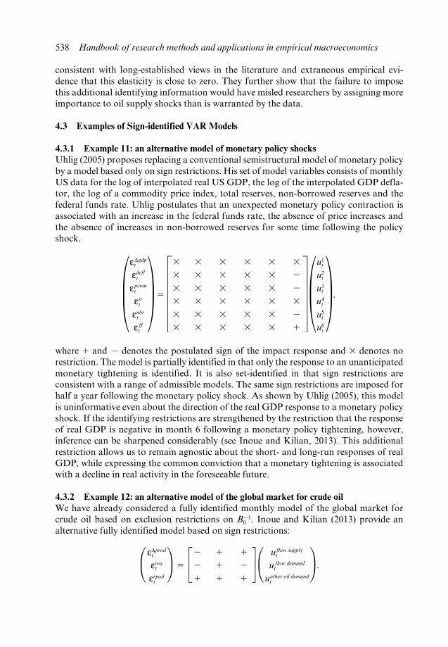
538 Handbook of research methods and applications in empirical macroeconomics
consistent with long- established views in the literature and extraneous empirical evi-dence that this elasticity is close to zero. They further show that the failure to impose this additional identifying information would have misled researchers by assigning more importance to oil supply shocks than is warranted by the data.
4.3 Examples of Sign- identified VAR Models
4.3.1 Example 11: an alternative model of monetary policy shocksUhlig (2005) proposes replacing a conventional semistructural model of monetary policy by a model based only on sign restrictions. His set of model variables consists of monthly US data for the log of interpolated real US GDP, the log of the interpolated GDP defla-tor, the log of a commodity price index, total reserves, non- borrowed reserves and the federal funds rate. Uhlig postulates that an unexpected monetary policy contraction is associated with an increase in the federal funds rate, the absence of price increases and the absence of increases in non- borrowed reserves for some time following the policy shock.
¶eDgdpt
edeflt
epcomt
etrt
enbrt
e fft
∂ 5 F3 3 3 3 3 3
3 3 3 3 3 2
3 3 3 3 3 2
3 3 3 3 3 3
3 3 3 3 3 2
3 3 3 3 3 1
V ¶u1t
u2t
u3t
u4t
u5t
u6t
∂ .
where 1 and 2 denotes the postulated sign of the impact response and 3 denotes no restriction. The model is partially identified in that only the response to an unanticipated monetary tightening is identified. It is also set- identified in that sign restrictions are consistent with a range of admissible models. The same sign restrictions are imposed for half a year following the monetary policy shock. As shown by Uhlig (2005), this model is uninformative even about the direction of the real GDP response to a monetary policy shock. If the identifying restrictions are strengthened by the restriction that the response of real GDP is negative in month 6 following a monetary policy tightening, however, inference can be sharpened considerably (see Inoue and Kilian, 2013). This additional restriction allows us to remain agnostic about the short- and long- run responses of real GDP, while expressing the common conviction that a monetary tightening is associated with a decline in real activity in the foreseeable future.
4.3.2 Example 12: an alternative model of the global market for crude oilWe have already considered a fully identified monthly model of the global market for crude oil based on exclusion restrictions on B21
0 . Inoue and Kilian (2013) provide an alternative fully identified model based on sign restrictions:
° eDprodt
ereat
erpoilt
¢ 5 £2 1 1
2 1 2
1 1 1
§ ° uflow supplyt
u flow demandt
uother oil demandt
¢ .
HASHIMZADE 9780857931016 CHS. 22-23 (M3110).indd 538HASHIMZADE 9780857931016 CHS. 22-23 (M3110).indd 538 01/07/2013 10:3101/07/2013 10:31
Structural vector autoregressions 539
Here the required signs of each element of B210 have been indicated by 1 and 2. Flow
supply shocks are normalized to correspond to supply disruptions. An unanticipated flow supply disruption causes oil production to fall, the real price of oil to increase, and global real activity to fall on impact. An unanticipated increase in the flow demand for oil driven by the global business cycle causes global oil production, global real activity and the real price of oil to increase on impact. Other positive oil demand shocks (such as shocks to oil inventory demand driven by forward- looking behavior) cause oil pro-duction and the real price of oil to increase on impact and global real activity to fall. In addition, the impact price elasticity of oil supply is bounded above by 0.025, as suggested by Kilian and Murphy (2012). This bound is consistent with widely held views among oil economists that the short- run price elasticity of oil supply is close to zero. The elasticity in question can be expressed as the ratio of two impact responses, making it straight-forward to discard draws that violate that restriction. Finally, following Baumeister and Peersman (2012) the real price of oil is restricted to be positive for the first year in response to unanticipated oil supply disruptions and in response to positive oil demand shocks.
5 ALTERNATIVE STRUCTURAL VAR APPROACHES
VAR models identified by sign restrictions are the most popular alternative to VAR models identified by short- run or long- run exclusion restrictions, but not the only alter-native. Discomfort with semistructural models of monetary policy in particular has stimulated the development of two more methodologies. It has been noted, in particular, that the sequences of policy shocks identified by such models do not always correspond to common perceptions of when policy shocks occurred. For example, Rudebusch (1998) compares estimates of monetary policy shocks from semistructural VAR models to financial market measures of policy shocks and finds little correspondence. He views this as evidence against the identifying assumptions employed in semistructural VAR models of monetary policy (also see Cochrane and Piazzesi, 2002).
5.1 Financial Market Shocks
This critique stimulated a new identification method by Faust et al. (2004) who iden-tify monetary policy shocks in monthly VAR models based on high- frequency futures market data. Using the prices of daily federal funds futures contracts, they measure the impact of the surprise component of Federal Reserve policy decisions on the expected future trajectory of interest rates. It is shown how this information can be used to iden-tify the effects of a monetary policy shock in a standard VAR. This alternative approach to identification is quite different from the conventional identifying restrictions in monetary policy VAR models in that it dispenses with the exclusion restrictions used in semistructural models of monetary policy.
Faust et al.’s procedure involves two key steps: first, they use the futures market to measure the response of expected future interest rates to an unexpected change in the Federal Reserve’s target rate. Specifically, they treat the change in the futures rate on the day on which a change in the Fed’s target federal funds rate is announced as a measure
HASHIMZADE 9780857931016 CHS. 22-23 (M3110).indd 539HASHIMZADE 9780857931016 CHS. 22-23 (M3110).indd 539 01/07/2013 10:3101/07/2013 10:31
540 Handbook of research methods and applications in empirical macroeconomics
of the change in market expectations. This interpretation requires that risk premia remain unchanged. Faust et al. further postulate that this change in expectations is due to the policy shock only. In other words, no other news moves the market on that day and the policy announcement itself does not reveal information about other structural shocks. In the second step, they impose that the impulse responses of the funds rate to the monetary policy shock in the VAR model must match the response measured from the futures data.
While these two steps are conceptually straightforward, carefully implementing them in practice requires dealing with several complications. Measuring the response of the funds rate to policy shocks in the futures data requires taking account of several peculiar aspects of the futures market and testing the validity of the underlying assumptions. Moreover, the information from the futures market only set- identifies the structural VAR model. The most striking implication of set identification is that one must give up on point estimation of the structural responses and focus on confidence intervals instead, similar to classical inference in sign- identified VAR models.
In their empirical analysis, Faust et al. find that the usual recursive identification of monetary policy shocks is rejected, as is any identification that insists on a monetary policy shock having no effect on prices contemporaneously. This confirms our earlier concerns with semistructural monetary policy VAR models. Their identification also eliminates the price puzzle – the finding in the benchmark recursive identification that the impulse response of prices first rises slightly but significantly, before falling. Faust et al. neverthe-less find that only a small fraction of the variance of output can be attributed to monetary policy shocks, as has been shown by the sign- identification methodology in Faust (1998).
D’Amico and Farka’s (2011) analysis of stock market and interest rate data takes this approach a step further. Rather than just estimating the response of stock returns to monetary policy shocks identified from high- frequency data, they propose a VAR methodology for estimating simultaneously the response of stock returns to policy deci-sions and the Federal Reserve’s contemporaneous reaction to the stock market. Their methodology has broad applicability when modeling asset prices. D’Amico and Farka’s approach involves two steps. In the first step, the response of the stock market to policy shocks is estimated outside the VAR model by measuring changes in intraday S&P500 futures prices immediately before and after policy announcements. The monthly policy shock is obtained by summing the intraday shocks over the course of a given month. In the second step, D’Amico and Farka impose that external estimate when estimating the response of the federal funds rate to stock returns in a monthly VAR model.
5.2 Identification by Heteroskedasticity
Rigobon (2003) develops yet another method for solving the VAR identification problem based on the heteroskedasticity of the structural shocks. Heteroskedasticity may arise, for example, as a result of financial crises. In the baseline model, Rigobon considers heteroskedasticity that can be described as a two- regime process and shows that the structural parameters of the system are just identified. He also discusses identi-fication under more general conditions such as when there are more than two regimes, when common unobservable shocks exist, and situations in which the nature of the het-eroskedasticity is misspecified.
HASHIMZADE 9780857931016 CHS. 22-23 (M3110).indd 540HASHIMZADE 9780857931016 CHS. 22-23 (M3110).indd 540 01/07/2013 10:3101/07/2013 10:31
Structural vector autoregressions 541
For expository purposes recall the two- equation model of demand and supply based on price and quantity data. All lags have been suppressed for notational convenience:
aept
eqtb 5 c 1 b
a 1d au1
t
u2tb.
Under the standard assumption of unconditional homoskedasticity, it can be shown that the reduced- form error covariance matrix is:
Se 51
(1 2 ab)2 cb2s22 1 s2
1 bs22 1 as2
1# s2
2 1 a2s21d ,
where s21 and s2
2 denote the variance of the first and the second structural shock. There are three moments in four unknowns (a, b, s2
1, s22), so without further assumptions such
as a 5 0 or b 5 0 it is not possible to identify the structural shocks from the data in this baseline model. This is the basic identification problem discussed throughout this survey.
Now suppose that there are two regimes in the variances of the structural shocks. Further suppose that the difference between regimes is that in one regime the uncondi-tional variance of the supply shock increases relative to the unconditional variance of the demand shocks, while the parameters a and b remain unchanged across regimes. This variance shift suffices to approximate the slope of the demand curve.
As a result of the regime shift, we obtain two expressions of the variance–covariance matrix, one for each regime r [ {1, 2} :
Se,r 51
(1 2 ab)2 cb2s22,r 1 s2
1,r bs22,r 1 as2
1,r# s2
2,r 1 a2s21,rd .
This means that there are now six moments in six unknowns, allowing us to solve for all six structural parameters (a, b, s2
1, 1, s22, 1, s2
1, 2, s22, 2) without restricting a or b. Rigobon
(2003) applies this methodology to the problem of characterizing the contemporane-ous relationship between the returns on Argentinean, Brazilian and Mexican sovereign bonds – a case in which standard identification methodologies do not apply. Rigobon’s approach is of particular interest for modeling asset prices because instantaneous feed-back must be assumed when trading is near- continuous. It is not without serious limita-tions, however. Not only is there uncertainty about the existence, number, and timing of the variance regimes, but in practice we are not likely to know whether a high volatility regime is caused by a relative increase in the volatility of demand shocks or of supply shocks, without assuming the answer to the identification question. This means that we do not know whether we are identifying the supply curve or the demand curve, which is the central question of interest. This problem is particularly apparent in modeling the global market for crude oil. Researchers have proposed competing views of what increased oil price volatility in the 1970s and Rigobon’s methodology would not be able to tell us, which view is supported by the data. This concern is less of an issue if the shock of interest can be associated with one variable only, as would be the case when modeling monetary policy shocks within a policy reaction function.
The latter case is discussed in Lanne and Lütkepohl (2008). Lanne and Lütkepohl
HASHIMZADE 9780857931016 CHS. 22-23 (M3110).indd 541HASHIMZADE 9780857931016 CHS. 22-23 (M3110).indd 541 01/07/2013 10:3101/07/2013 10:31

542 Handbook of research methods and applications in empirical macroeconomics
propose a test of over-identifying restrictions within the structural VAR framework of Bernanke and Mihov (1998). Their test exploits evidence of structural change in the variance–covariance matrix of the reduced- form shocks. As in Rigobon’s work, the main-tained assumption is that the autoregressive parameters are time invariant. Volatility in the shocks is significantly higher during the Volcker period than the post- Volcker period. This volatility change may be used to test alternative models of the money market. Based on monthly US data for 1965 to 1996, Lanne and Lütkepohl conclude that a model in which monetary policy shocks are associated with shocks to non- borrowed reserves is rejected by the data, whereas a model in which the Federal Reserve accommodates demand shocks to total reserves is not rejected.
In closely related work, Lanne et al. (2010) address the issue of how to detect struc-tural changes in the volatility of the VAR errors in the data. They consider the important special case of volatility shifts that follow a Markov regime switching model (see Sims and Zha, 2006). Identification is achieved by assuming that the shocks are orthogonal across states and that only the variances of the shocks change across states, while the other model parameters remain unaffected. Modeling the reduced- form errors as a Markov regime switching model provides data- dependent estimates of the dates of vola-tility shifts, conditional on the assumed number of regimes.
Finally, a related identification methodology for vector autoregressions with non- normal residuals has also been discussed by Lanne and Lütkepohl (2010). It is well known that VAR regression errors are frequently non- normal. These errors may be modeled as a mixture of normal distributions. That assumption is useful, for example, when the reduced- form error distribution has heavy tails and a tendency to generate out-liers. In that case, one may think of the outliers as being generated by a distribution dif-ferent from the distribution of the other observations and identification may be obtained by heteroskedasticity across regimes. Unlike in Rigobon’s approach, the unconditional error distribution remains homoskedastic, however, and the regime switches in the model are generated endogeneously.
5.3 Identification in the Presence of Forward- looking Behavior
It is important to stress that standard VAR models of monetary policy are concerned with responses to unanticipated policy shocks. They have nothing to say about the effects of anticipated monetary policy shocks. For further discussion see also Leeper et al. (1996), Bernanke and Mihov (1998) and Christiano et al. (1999). The anticipation of shocks is an even greater concern when modeling fiscal policy shocks or productivity shocks and requires fundamental modifications in the analysis. The mere possibility of forward- looking behavior greatly complicates the identification of structural shocks in VAR models.
The maintained assumption in structural VAR analysis is that the structural data- generating process can be represented as a VAR model. In other words, we start with the structural VAR representation with the objective of recovering the structural VMA rep-resentation. Suppose that instead we started with the premise that the data- generating process is of the form of the structural VMA
yt 5 Q(L)ut.
HASHIMZADE 9780857931016 CHS. 22-23 (M3110).indd 542HASHIMZADE 9780857931016 CHS. 22-23 (M3110).indd 542 01/07/2013 10:3101/07/2013 10:31
Structural vector autoregressions 543
where the number of variables equals the number of structural shocks. Not every struc-tural VMA has an equivalent structural VAR representation. Expressing the structural VMA process as a structural VAR process of the form
Q(L)21yt 5 B(L)yt 5 ut
requires all roots of det(Q(L)) to be outside the unit circle. This condition rules out models with unit roots in the moving average polynomial, for example, because in that case the moving average polynomial is not invertible. This situation will arise when the data have been overdifferenced. Such cases can be handled by transforming the data appropriately. A more serious complication is that the moving average roots may be inside the unit circle. In this case, the model is said to be non- fundamental. Such repre-sentations imply the same autocovariance structure as the fundamental representation, but the underlying structural shocks cannot be recovered from current and past observa-tions of the variables included in the VAR model even asymptotically. Consequently, when the economic model does not guarantee fundamentalness, standard structural impulse response analysis may be misleading (see Lippi and Reichlin, 1993, 1994).
How concerned we should be with that possibility depends on whether non- fundamental representations can be shown to arise in economic theory. In this regard, Hansen and Sargent (1991) illustrated that non- fundamental representations may arise in rational expectations models when agents respond to expectational variables that are not observable to the econometrician. This result suggests extreme caution in interpret-ing structural VAR models when the VAR information set is smaller than that of the agents making economic decisions in the real world, as would typically be the case in models with forward- looking behavior. If we think of asset prices containing informa-tion about expected movements in real macroeconomic aggregates beyond the informa-tion in the lagged macroeconomic aggregates, for example, then a VAR including only real macroeconomic aggregates would be misspecified. In particular, we would not be able to recover the true structural shocks of this economy from the reduced- form VAR representation under any possible identification scheme. If we simply ignored this problem, we would end up identifying seemingly structural shocks without economic meaning. For further discussion see Lippi and Reichlin (1993, 1994), Blanchard and Quah (1993), Forni et al. (2009) and Leeper et al. (2011).
A formal test designed to detect non- fundamentalness of this type in a given structural VAR model was proposed by Giannone and Reichlin (2006). Giannone and Reichlin showed that Granger causality from a set of potentially relevant variables that are omitted from the baseline VAR model to the variables already included in the baseline model implies that the structural shocks in the baseline model are not fundamental. Under weak conditions, adding previously omitted Granger causal variables to the VAR model may eliminate this informational inefficiency. Even a model modified in this fashion, however, need not be properly identified. One problem is that there may be expectational variables that affect agents’ behavior which are not observable. Thus, passing the Giannone and Reichlin test is necessary, but not sufficient for ruling out identification problems in the structural model. The other problem is that the inclusion of previously omitted Granger causal variables may undermine conventional identifica-tion strategies. For example, it may seem that the problem of non- fundamental VAR
HASHIMZADE 9780857931016 CHS. 22-23 (M3110).indd 543HASHIMZADE 9780857931016 CHS. 22-23 (M3110).indd 543 01/07/2013 10:3101/07/2013 10:31

544 Handbook of research methods and applications in empirical macroeconomics
representations could be mitigated, if not avoided altogether, by simply augmenting the set of VAR variables with forward- looking variables such as asset prices, survey meas-ures of expectations, or professional forecasts. This strategy, however, may invalidate commonly used approaches to identifying monetary policy shocks. Consider a semi-structural model of monetary policy of the type discussed earlier. If we add stock prices to the list of variables the Federal Reserve responds to in setting interest rates, we are implicitly assuming that stock prices do not respond instantaneously to interest rates, which does not seem plausible. If we order stock prices below the interest rate, on the other hand, we prevent the Federal Reserve from responding to a variable that matters for agents’ economic decisions and hence should matter to the Federal Reserve. Thus, the presence of forward- looking variables often requires additional modifications in the identification strategy.
Only recently, VAR models have been adapted to allow for forward- looking behav-ior of some form. Such extensions are non- trivial. Here we consider three illustrative examples. None of the examples provides a generic solution to the problem of modeling forward- looking behavior, but they illustrate that at least in special cases these problems may be overcome.
5.3.1 Example 13: shocks to expectations about future oil demand and oil supply conditions
The first example is a model of the global spot market for crude oil proposed by Kilian and Murphy (2013). Identification is based on a four- variable model including the change in above- ground global inventories of crude oil in addition to the three variables already included in Kilian and Murphy (2012). The key observation is that any change in expectations about future oil demand and oil supply conditions not already captured by flow demand shocks and flow supply shocks must be reflected in a shift in the demand for oil inventories, conditional on past data. By including these inventories (the change of which is denoted by Dinv) in the model and simultaneously identifying all shocks that move inventories, it becomes possible to identify the effect of shifts in expectations without having to measure expectations explicitly. The model is identified by a combina-tion of sign restrictions on the impact responses, bounds on the impact price elasticities of oil demand and of oil supply, and dynamic sign restrictions on the responses to unex-pected flow supply disruptions. The impact sign restrictions are:
± eDprodt
ereat
erpoilt
eDinvt
≤ 5 ≥2 1 1 3
2 1 2 3
1 1 1 3
3 3 1 3
¥ ± uflow supplyt
u flow demandt
uspeculative demandt
uother oil demandt
≤ .
In other words, on impact, a negative flow supply shock shifts the supply curve to the left along the demand curve, resulting in a decline in the quantity and an increase in the price of oil, which causes real activity to decline. A positive flow demand shock is associated with increased real activity. Quantity and price increase, as the demand curve shifts to the right along the supply curve, while real activity increases by construction. The inventory responses to flow supply and flow demand shocks are ambiguous a priori
HASHIMZADE 9780857931016 CHS. 22-23 (M3110).indd 544HASHIMZADE 9780857931016 CHS. 22-23 (M3110).indd 544 01/07/2013 10:3101/07/2013 10:31
Structural vector autoregressions 545
and hence remain unrestricted. A positive speculative demand shock reflecting expecta-tions of a tightening oil market is associated with an increase in inventories and in the real price of oil by construction. The accumulation of inventories requires oil production to increase and oil consumption (and hence real activity) to decline. Effectively, this model further decomposes the other oil demand shock in Inoue and Kilian (2013) into a speculative component driven by shifts in expectations and a residual containing only the remaining idiosyncratic oil demand shocks. In addition, the model imposes that the impact price elasticity of oil supply is bounded above and that the impact price elasticity of oil demand (defined to incorporate the inventory response) is restricted to be negative and smaller in magnitude than the long- run price elasticity of oil demand which can be estimated from cross- sectional data. Both elasticities can be expressed as ratios of struc-tural impulse responses on impact. Finally, the model imposes that the sign restrictions on the responses to a flow supply shock remain in effect for one year.
It may seem that this oil market model is incomplete in that it excludes the price of oil futures contracts, which is commonly viewed as an indicator of market expectations about future oil prices. This is not the case. The spot market and the futures market for oil are two distinct markets linked by an arbitrage condition. Thus, if there is speculation in the oil futures market, by arbitrage there should be speculation in the spot market reflected in increased inventory demand (see Alquist and Kilian, 2010). Not only does economic theory imply that oil futures prices are redundant in this model of the spot market, but one can use the Giannone and Reichlin (2006) test to show that the oil futures spread does not Granger cause the variables in the Kilian and Murphy model, consistent with the view that the structural shocks are fundamental.9
5.3.2 Example 14: anticipated technology shocksA second example of a structural VAR model of forward- looking behavior is Barsky and Sims (2011) who focus on expectations about future aggregate productivity. They pos-tulate that the log of aggregate productivity, At, is characterized by a stochastic process driven by two structural shocks. The first shock is the traditional surprise technology shock, which impacts the level of productivity in the same period in which agents observe it. The second shock reflects information about future technology and is defined to be orthogonal to the first shock.10 The two shocks jointly account for all variation in At. The two structural shocks are identified as follows:
At 5 [B11 (L)B12 (L) ]au1t
u2tb
where B12 (0) 5 0 such that only u1t affects current productivity, making u2t the future technology shock. Effectively, Barsky and Sims treat At as predetermined with respect to the rest of the economy. This identifying assumption leaves a wide range of possible choices for u2t. In practice, u2t is identified as the shock that best explains future move-ments in At11, . . . , At1H, not accounted for by its own innovation, where H is some finite horizon. This approach, of course, amounts to constructing the best possible case for the role of shocks to expectations rather than necessarily the most likely case.
The estimated VAR model includes a total factor productivity series as well as selected macroeconomic aggregates. At is ordered first. The procedure is implemented by
HASHIMZADE 9780857931016 CHS. 22-23 (M3110).indd 545HASHIMZADE 9780857931016 CHS. 22-23 (M3110).indd 545 01/07/2013 10:3101/07/2013 10:31
546 Handbook of research methods and applications in empirical macroeconomics
constructing candidate solutions of the form PD, where P denotes the lower triangular Cholesky decomposition of Se and D a conformable orthogonal matrix, as in the case of sign- identified VAR models. The ability of a shock to explain future movements of the data is measured in terms of the forecast- error variance decomposition. Because the contribution of the second shock to the forecast error variance of At depends only on the second column of A21
0 , Barsky and Sims choose the second column, g, to solve the optimization problem:
g* 5 arg maxaH
h50W12 (h),
subject to the first element of g being zero and grg 5 1, where Wij(h) denotes the share of the forecast error variance of variable i attributable to structural shock j at horizon h expressed in terms of the structural parameters of the model (also see Lütkepohl, 2005).
5.3.3 Example 15: anticipated tax shocksIn related work, Leeper et al. (2011) address the problem of anticipated tax shocks in the context of the model of Blanchard and Perotti (2002). Although Blanchard and Perotti as part of a sensitivity analysis relaxed the assumption of no foresight in their baseline model, they only investigated a very limited form of tax foresight involving one quarter of anticipation. Clearly, there is no compelling reason for agents not to be more forward- looking.
Leeper et al. propose a more general approach. Their starting point is the observation that the differential US Federal tax treatment of municipal and treasury bonds embeds news about future taxes. The current spread, st, between municipal bonds and treasury bonds may be viewed as an implicit tax rate. This implicit tax rate is a weighted average of discounted expected future tax rates and should respond immediately to news about expected future tax changes. This motivates treating st as a variable containing expecta-tions of future tax shocks. Assuming market efficiency, the implicit tax rate reveals the extent to which agents do or do not have foresight. A simple test is whether st contains useful predictive information for the variables modeled by Blanchard and Perotti. Leeper et al. demonstrate that st Granger causes the variables in Blanchard and Perotti’s VAR model, indicating that this model is not fundamental. Their solution is to augment the model of Blanchard and Perotti with data on the spread, s, resulting in the four- variable system:
± etaxt
egovt
egdpt
est
≤ 5 ± 2.08egdpt 1 utax
t
dutaxt 1 ugov
t
eetaxt 1 fegov
t 1 ugdpt
getaxt 1 hegov
t 1 iegdpt 1 us
t
≤They add the identifying assumption that news contained in the interest rate spread,
ust, has no direct effect on current output, tax revenue and spending. The resulting
structural VAR model can be used to construct responses both to unanticipated and anticipated tax revenue shocks. Leeper et al. show that their model produces markedly different impulse response estimates from Blanchard and Perotti’s model and suggests that agents’ foresight may extend as far as five years.
HASHIMZADE 9780857931016 CHS. 22-23 (M3110).indd 546HASHIMZADE 9780857931016 CHS. 22-23 (M3110).indd 546 01/07/2013 10:3101/07/2013 10:31

Structural vector autoregressions 547
6 STRUCTURAL VAR MODELS AND DSGE MODELS
Both structural VAR models and DSGE models were developed in response to the perceived failure of traditional large- scale macroeconometric models in the 1970s. Proponents of DSGE models responded to this evidence by developing fully structural models that facilitated policy analysis, but at the expense of requiring strong assump-tions about market structures, functional forms and about the exogeneity and dynamic structure of the underlying forcing variables. Proponents of structural VAR models responded by proposing dynamic simultaneous equation models that required minimal assumptions about the dynamics of the model variables, no assumptions about the exo-geneity of any variable, and minimal assumptions about the structure of the economy. They dispensed in particular with the imposition of cross- equation restrictions in an effort to make the structural VAR model robust to alternative ad hoc modeling choices.
An obvious question is under what conditions these modeling approaches are compat-ible and under what conditions one might be able to learn from one approach about the other. This has been less of a concern for DSGE proponents (who often reject the struc-tural VAR approach on a priori grounds) than for proponents of the structural VAR approach, some of whom have viewed results from structural VAR models as informa-tive for DSGE modeling (see, for example, Galí, 1999). Recent research has shown that comparisons of structural VAR estimates with DSGE models are not straightforward:
● Not every DSGE model will have a structural VAR representation. Fernandez- Villaverde et al. (2007) discuss invertibility conditions that must be met for data from a DSGE model to have a structural VAR representation. Whether this fact is a concern for structural VAR modeling depends on whether we view the excluded DSGE models as practically relevant. Moreover, Sims (2012) shows that there may exist situations in which a model has a non- invertible VAR representation, yet structural VAR models nevertheless perform reliably.
● Conversely, not every structural VAR model will correspond to an existing DSGE model. This does not necessarily mean that the structural VAR model lacks theoretical support. It may also reflect our inability to write down and solve more articulated theoretical models.
● The state- space representation of a DSGE model’s log- linearized equilibrium often can be expressed in terms of a vector autoregressive moving average (VARMA) process for the observable DSGE model variables. It rarely will take the form of a finite- order VAR process. Integrating out some of the model variables will further affect the nature of the reduced- form VARMA representation. Under suitable conditions, the resulting VARMA model for the observables can be inverted and expressed as a VAR(`) model, which in turn can be approximated by a sequence of finite- order VAR(k) processes, where k increases with the sample size at a suitable rate. The use of an autoregressive sieve approximation has important implications for lag order selection and for statistical inference in the implied VAR(k) model (see, for example, Inoue and Kilian, 2002).
An obvious concern in practice is how well a VAR(`) model may be approxi-mated by a VAR(k) in finite samples. One important area of current research is how to select k. The answer depends in part on which aspect of the DSGE model
HASHIMZADE 9780857931016 CHS. 22-23 (M3110).indd 547HASHIMZADE 9780857931016 CHS. 22-23 (M3110).indd 547 01/07/2013 10:3101/07/2013 10:31
548 Handbook of research methods and applications in empirical macroeconomics
we are interested in. This is an open area of research. Simulation evidence suggests that in some cases the VAR(k) approximation to the VAR(`) process may be poor for realistic sample sizes for any feasible choice of k. This problem can be severe when the underlying DSGE model has a VARMA representation with a high moving average root.
● The existence of an approximate reduced- form VAR(k) representation is a nec-essary, but not a sufficient condition for the existence of a structural VAR(k) representation. One additional condition is that the number of shocks in the DSGE model must match the number of shocks in the VAR model. Recall that we postulated that Su is of full column rank. This means that there must be as many shocks as variables in the VAR model. Many DSGE models have fewer shocks than variables. For example, a textbook real business cycle model has only one technology shock, so, when fitting a VAR to output, investment and consumption data generated from this DSGE model, Su would be of reduced rank if the DSGE model were correct. Clearly, the DSGE model and VAR model specifications are incompatible in that case. Users of DSGE models have responded to this problem by either adding ad hoc noise without structural interpretation (such as measure-ment error) or by augmenting the number of economic shocks in the DSGE model. Examples include preference shocks, fiscal shocks and monetary shocks. This can be problematic if the additional shocks in the DSGE model have no clear struc-tural interpretation or involve questionable exogeneity assumptions.
Another additional condition is that the restrictions imposed in identifying the structural shocks in the VAR model must be consistent with the underlying DSGE model structure. This is rarely the case when using short- run exclusion restrictions, so caution must be exercised in comparing results from DSGE and structural VAR models. This point was first illustrated by Keating (1990) in the context of a simple rational expectations model. The use of long- run restrictions as in Galí (1999) circumvents this problem in part, but it requires the user to take a strong stand on the presence of unit roots and near- unit roots, it requires the DSGE model to be consistent with these assumptions, it focuses on one shock at the expense of others, and it suffers from its own limitations as discussed earlier. Simulation evidence on the efficacy of this approach is mixed (see, for example, Gust and Vigfusson, 2009). Perhaps the best hope for matching structural VAR models and DSGE models is the use of sign restrictions. Canova and Paustian (2011) report considerable success in recovering responses generated by DSGE models with the help of sign- identified structural VAR models. They stress the importance of not being too agnostic about the identification, however. It is generally easier to recover the underlying population responses when more variables are restricted, for a given number of identified shocks, or when more structural shocks are identified in the VAR model. Moreover, models based on weak identifying restrictions may become unreliable when the variance of the shock in question is small in population. This conclusion is further reinforced by the discussion in Kilian and Murphy (2012) of the dangers of relying on excessively agnostic sign- identified VAR models.
● The earlier comments about forward- looking behavior continue to apply. As noted by Sims (2012), when the data are generated by a DSGE model in which shocks are anticipated by the agents, there is a missing state variable in the structural VAR
HASHIMZADE 9780857931016 CHS. 22-23 (M3110).indd 548HASHIMZADE 9780857931016 CHS. 22-23 (M3110).indd 548 01/07/2013 10:3101/07/2013 10:31
Structural vector autoregressions 549
representation of the observables, and structural VAR models will be unable to recover the true structural shocks. There is evidence that this problem need not be fatal, however. Even when the conditions for the invertibility of the state- space representation fail, the degree of misspecification of the structural VAR responses may be small.
This discussion highlights that in general caution must be exercised in comparing structural VAR and DSGE model estimates. Interest in such comparisons has further increased in recent years, as Bayesian estimation methods have facilitated the estimation of the state- space representation of DSGE models, making it possible to dispense with VAR models in estimating structural impulse responses. At the same time, there has been increasing recognition that DSGE models are not only sensitive to ad hoc modeling choices, but often suffer from weak identification of the structural parameters. Unless we are very confident about the adequacy of the DSGE model structure, estimates of DSGE models may be misleading, and calibration of the model parameters will be preferable. Moreover, even if the model structure is adequate, structural parameter estimates may be sensitive to the choice of priors. Thus, both the structural VAR approach and the DSGE model approach have to be used with care and the best we can hope for is that both types of models paint a similar picture.
7 CONCLUSION
In addition to continued innovation in the area of the identification of structural shocks from VAR models, recent years have witnessed a number of generalizations of the underlying reduced- form VAR framework. One of the main concerns in the VAR literature we already alluded to is that policy rules and more generally the structure of the economy may evolve over time. One possibility is that structural changes occur infrequently, resulting in occasional breaks in the data that can be handled by split-ting the sample. For example, Boivin and Giannoni (2006) consider the possibility that the Great Moderation was caused by a one- time break in the volatilities of the VAR shocks as opposed to improved monetary policy responses. They suggest that, if only the volatilities of the shocks changed during the Great Moderation, structural response functions estimated on pre- break data – after suitable normalizations to control for the magnitude of the shocks – should be identical to structural impulse responses estimated on post- break data, whereas changes in the shape of the response functions would be an indication of a change in the transmission mechanism. Inoue and Rossi (2011), however, document that time- invariant impulse response shapes are not sufficient for structural stability because structural breaks in the autoregressive slope parameters may have off-setting effects on the impulse response functions. Moreover, if there are changes in the shape of the impulse response functions, it is not possible to infer from these changes which parameters in the structural model changed. In particular, it is difficult to infer whether these changes are associated with better policy rules or with other instabilities in the structural model.
A more pernicious form of structural change is associated with smoothly time- varying model parameters. In some cases, such temporal instability may be modeled within a
HASHIMZADE 9780857931016 CHS. 22-23 (M3110).indd 549HASHIMZADE 9780857931016 CHS. 22-23 (M3110).indd 549 01/07/2013 10:3101/07/2013 10:31
550 Handbook of research methods and applications in empirical macroeconomics
linear VAR framework. For example, Edelstein and Kilian (2009) showed how time variation in the share of energy expenditures in total consumption may be modeled within a linear VAR framework by redefining energy price shocks in terms of shocks to the purchasing power of consumers. A similar approach was taken by Ramey and Vine (2011) in modeling gasoline price rationing. An alternative approach pioneered by Primiceri (2005), Benati (2008), Canova and Gambetti (2009), and Baumeister and Peersman (2012) has been to allow for explicit smooth time variation in the parameters of the structural VAR model. The development of structural TVP- VAR models is chal-lenging because the identifying restrictions themselves may be time- varying. Structural VAR models have also been extended to allow for more specific non- linearities such as regime- switching, threshold non- linearities, or GARCH in mean (see, for example, Elder and Serletis, 2010). Not all non- linearities lend themselves to structural VAR analysis, however. For example, Kilian and Vigfusson (2011a, 2011b) show that certain models involving asymmetric transmissions of shocks may not be represented as structural VAR models. They propose an alternative non- VAR representation of dynamic asymmetric structural models.
A second development in recent years has been the integration of results from the literature on data- dimension reduction in forecasting from large cross- sections. One example is the development of factor augmented VAR (FAVAR) models as in Bernanke et al. (2005) or Stock and Watson (2005). An alternative approach has been the use of large- scale Bayesian VAR models as in Banbura et al. (2010). Both model frameworks allow the user to generate impulse responses for a much larger set of variables than tra-ditional VAR models. A third development has been the increased popularity of panel VAR models (see, for example, Canova, 2007).
These developments illustrate that there is much life left in the research program started by Sims (1980a, 1980b). As with all methodologies, structural vector autoregres-sions can be powerful tools in the right hands, yet potentially misleading if used blindly. Credible applications require careful consideration of the underlying economic struc-ture. Although not every problem can be cast in a structural VAR framework, structural VAR models are likely to remain an important tool in empirical macroeconomics. There is no indication that DSGE models, in particular, are ready to take the place of structural vector autoregressions. Both approaches have their distinct advantages and disadvan-tages, and it remains up to the researcher to decide which class of models is more appro-priate for a given question.
NOTES
* I thank Ron Alquist, Christiane Baumeister, Fabio Canova, Carlo Favero, Nikolay Gospodinov, Ana María Herrera, Helmut Lütkepohl, and Barbara Rossi for helpful comments on an earlier draft.
1. It is worth noting that, in general, structural shocks do not correspond to particular model variables. For example, in a VAR system consisting of only price and quantity, we can think of a demand shock and a supply shock each shifting prices and quantities. In fact, if price and quantity variables were mechanically associated with price and quantity shocks, this would be an indication that the proposed model is not truly structural.
2. Standard software provides built- in functions for generating the Cholesky decomposition of Se. 3. Christiano et al. (1999) prove that alternative orderings of eDgdp
t and ept will leave u3
t unaffected, provided the model is recursive.
HASHIMZADE 9780857931016 CHS. 22-23 (M3110).indd 550HASHIMZADE 9780857931016 CHS. 22-23 (M3110).indd 550 01/07/2013 10:3101/07/2013 10:31
Structural vector autoregressions 551
4. The Bureau of Economic Analysis does not release monthly US real GDP data. Unofficial measures of monthly US real GDP constructed similarly to the official quarterly data have recently been provided by Macroeconomic Advisers, LLC. These time series for the time being are not long enough for estimating VAR models of monetary policy, however.
5. The price puzzle refers to the finding of a statistically significant increase in the price level in response to an unanticipated monetary tightening in models of this type. Sims (1992) suggested that this puzzle could be resolved by including global commodity prices as an indicator of future inflation in the model. This idea is reasonable because the Federal Reserve considers global commodity prices as a predictor of inflation. Hanson (2004), however, showed that there is little correlation between the ability of alternative measures of global commodity prices to predict inflation and to resolve the price puzzle. Indeed, subsequent research has shown that the price puzzle more often than not persists even after including global commodity prices in the VAR model, suggesting that the model remains misspecified.
6. The terminology of transitory shocks and permanent shocks is somewhat misleading in that any shock by construction involves a one- time disturbance only. A transitory shock, more precisely, is defined as a shock with purely transitory effects on the observables, whereas a permanent shock refers to a shock with permanent (or long- run) effects on the observables.
7. It can be shown that the results of Cochrane’s model would be exactly identical to the results from a model in which the transitory shock has no long- run effect on the level of income and consumption, pro-vided consumption follows a pure random walk. Such long- run restrictions will be discussed in section 3.
8. A generalization of the approach of Blanchard and Quah (1989) was proposed by King et al. (1991). King et al. consider a baseline model for output, consumption and investment. Unlike in Blanchard and Quah (1989), in their 3- variable VAR model all variables are driven by the same productivity shock in the long run. In other words, the model variables are cointegrated. King et al. are interested in using this model to differentiate between the three variables’ responses to the common productivity shock. One difficulty in models such as this one lies in finding an economically credible identification of the transitory shocks. Another difficulty lies in how to distinguish between multiple permanent shocks when dealing with larger VAR models.
9. One could have considered an alternative specification in which the oil futures spread replaces the change in crude oil inventories, but one- year oil futures contracts did not exist on a monthly basis prior to 1989, so this alternative specification would involve a much smaller sample size. Another advantage of the specification in Kilian and Murphy (2013) is that it remains equally valid even in the absence of an oil futures market (or when arbitrage for some reason is less than perfect). Nor would a model based on the oil futures spread allow the imposition of bounds on the oil demand elasticity.
10. Barsky and Sims refer to this shock as a news shock, following a terminology common in the recent macroeconomic literature. This is somewhat misleading in that news shocks have traditionally been defined as unexpected changes to observed aggregates (see, for example, Kilian and Vega, 2011). Rather the second shock captures expected changes in future productivity.
REFERENCES
Abraham, K.G and J.C. Haltiwanger (1995), ‘Real wages and the business cycle’, Journal of Economic Literature, 33, 1215–64.
Alquist, R. and L. Kilian (2010), ‘What do we learn from the price of crude oil futures?’, Journal of Applied Econometrics, 25, 539–73.
Banbura, M., D. Giannone and L. Reichlin (2010), ‘Large Bayesian vector autoregressions’, Journal of Applied Econometrics, 25, 71–92.
Barsky, R.B. and E.R. Sims (2011), ‘News shocks and business cycles’, Journal of Monetary Economics, 58, 273–89.
Baumeister, C. and L. Kilian (2012), ‘Real- time analysis of oil price risks using forecast scenarios’, mimeo, University of Michigan.
Baumeister, C. and G. Peersman (2012), ‘The role of time- varying price elasticities in accounting for volatility changes in the crude oil market’, Journal of Applied Econometrics, DOI: 10.1002/jae.2283.
Benati, L. (2008), ‘The “Great Moderation” in the United Kingdom’, Journal of Money, Credit and Banking, 40, 121–47.
Bernanke, B.S. (1986), ‘Alternative explanations of the money–income correlation’, Carnegie- Rochester Conference Series on Public Policy, 25, 49–99.
HASHIMZADE 9780857931016 CHS. 22-23 (M3110).indd 551HASHIMZADE 9780857931016 CHS. 22-23 (M3110).indd 551 01/07/2013 10:3101/07/2013 10:31
552 Handbook of research methods and applications in empirical macroeconomics
Bernanke, B.S. and A. Blinder (1992), ‘The federal funds rate and the channels of monetary transmission’, American Economic Review, 82, 901–21.
Bernanke, B.S. and J. Boivin (2003), ‘Monetary policy in a data- rich environment’, Journal of Monetary Economics, 50, 525–46.
Bernanke, B.S. and I. Mihov (1998), ‘Measuring monetary policy’, Quarterly Journal of Economics, 113, 869–902.
Bernanke, B.S., J. Boivin and P. Eliasz (2005), ‘Measuring monetary policy: a Factor Augmented Vector Autoregressive (FAVAR) approach’, Quarterly Journal of Economics, 120, 387–422.
Bernanke, B.S., M. Gertler and M. Watson (1997), ‘Systematic monetary policy and the effects of oil price shocks’, Brookings Papers on Economic Activity, 1, 91–142.
Blanchard, O.J. (1989), ‘A traditional interpretation of macroeconomic fluctuations’, American Economic Review, 79, 1146–64.
Blanchard, O.J. and R. Perotti (2002), ‘An empirical investigation of the dynamic effects of shocks to govern-ment spending and taxes on output’, Quarterly Journal of Economics, 117, 1329–68.
Blanchard, O.J. and D. Quah (1989), ‘The dynamic effects of aggregate demand and supply disturbances’, American Economic Review, 79, 654–73.
Blanchard, O.J. and D. Quah (1993), ‘The dynamic effects of aggregate demand and supply disturbances: reply’, American Economic Review, 83, 653–8.
Blanchard, O.J. and M.W. Watson (1986), ‘Are business cycles all alike?’, in R.J. Gordon (ed.), The American Business Cycle, Chicago, IL: NBER and Chicago Press, pp. 123–79.
Boivin, J. and M. Giannoni (2006), ‘Has monetary policy become more effective?’, Review of Economics and Statistics, 88, 445–62.
Canova, F. (2007), Methods for Applied Macroeconomic Research, Princeton, NJ: Princeton University Press.
Canova, F. and G. De Nicolo (2002), ‘Monetary disturbances matter for business fluctuations in the G- 7’, Journal of Monetary Economics, 49, 1131–59.
Canova, F. and L. Gambetti (2009), ‘Structural changes in the US economy: is there a role for monetary policy?’, Journal of Economic Dynamics and Control, 33, 477–90.
Canova, F. and E. Pappa (2007), ‘Price dispersions in monetary unions: the role of fiscal shocks’, Economic Journal, 117, 713–37.
Canova, F. and M. Paustian (2011), ‘Measurement with some theory: using sign restrictions to evaluate busi-ness cycle models’, Journal of Monetary Economics, 58, 345–61.
Canova, F., D. López- Salido and C. Michelacci (2010), ‘The effects of technology shocks on hours and output: a robustness analysis’, Journal of Applied Econometrics, 25, 755–73.
Christiano, L., M. Eichenbaum and C. Evans (1999), ‘Monetary policy shocks: what have we learned and to what end?’, in J.B Taylor and M. Woodford (eds), Handbook of Macroeconomics, vol. 1, Amsterdam: Elsevier/North Holland, pp. 65–148.
Chung, H. and E. Leeper (2007), ‘What has financed government debt?’, NBER Working Paper No. 13425.Cochrane, J.H. (1994), ‘Permanent and transitory components of GNP and stock prices’, Quarterly Journal of
Economics, 109, 241–65.Cochrane, J.H. and M. Piazzesi (2002), ‘The Fed and interest rates: a high- frequency identification’, American
Economic Review, 92, 90–95.Cooley, T.F. and S. LeRoy (1985), ‘Atheoretical macroeconometrics: a critique’, Journal of Monetary
Economics, 16, 283–308.Cushman, D.O. and T. Zha (1997), ‘Identifying monetary policy in a small open economy under flexible
exchange rates’, Journal of Monetary Economics, 39, 433–48.D’Amico, S. and M. Farka (2011), ‘The Fed and the stock market: an identification based on intraday futures
data’, Journal of Business and Economic Statistics, 29, 126–37.Davis, L.W. and L. Kilian (2011), ‘Estimating the effect of a gasoline tax on carbon emissions’, Journal of
Applied Econometrics, 26, 1187–1214.Dedola, L. and S. Neri (2007), ‘What does a technology shock do? A VAR analysis with model- based sign
restrictions’, Journal of Monetary Economics, 54, 512–49.Edelstein, P. and L. Kilian (2009), ‘How sensitive are consumer expenditures to retail energy prices?’, Journal
of Monetary Economics, 56, 766–79.Elder, J. and A. Serletis (2010), ‘Oil price uncertainty’, Journal of Money, Credit and Banking, 42, 1138–59.Faust, J. (1998), ‘The robustness of identified VAR conclusions about money’, Carnegie- Rochester Conference
Series on Public Policy, 49, 207–44.Faust, J. and E. Leeper (1997), ‘When do long- run identifying restrictions give reliable results?’, Journal of
Business Economics and Statistics, 15, 345–53.Faust, J., E. Swanson and J.H. Wright (2004), ‘Identifying VARs based on high frequency futures data’,
Journal of Monetary Economics, 51, 1107–31.
HASHIMZADE 9780857931016 CHS. 22-23 (M3110).indd 552HASHIMZADE 9780857931016 CHS. 22-23 (M3110).indd 552 01/07/2013 10:3101/07/2013 10:31
Structural vector autoregressions 553
Fernández- Villaverde, J., J.F. Rubio- Ramírez, T.J. Sargent and M.W. Watson (2007), ‘ABCs (and Ds) of understanding VARs’, American Economic Review, 97, 1021–26.
Forni, M., D. Giannone, M. Lippi and L. Reichlin (2009), ‘Opening the black box: structural factor models with large cross- sections’, Econometric Theory, 25, 1319–47.
Francis, N., M. Owyang, J.E. Roush and R. DiCecio (2010), ‘A flexible finite- horizon alternative to long- run restrictions with an application to technology shocks’, mimeo, Federal Reserve Bank of St Louis.
Fry, R. and A. Pagan (2011), ‘Sign restrictions in structural vector autoregressions: a critical review’, Journal of Economic Literature, 49, 938–60.
Fujita, S. (2011), ‘Dynamics of worker flows and vacancies: evidence from the sign restriction approach’, Journal of Applied Econometrics, 26, 89–121.
Galí, J. (1992), ‘How Well does the IS–LM model fit postwar US data?’, Quarterly Journal of Economics, 107, 709–38.
Galí, J. (1999), ‘Technology, employment, and the business cycle: do technology shocks explain aggregate fluctuations?’, American Economic Review, 89, 249–71.
Giannone, D. and L. Reichlin (2006), ‘Does information help recover structural shocks from past observa-tions?’, Journal of the European Economic Association, 4, 455–65.
Gospodinov, N. (2010), ‘Inference in nearly nonstationary SVAR models with long- run identifying restric-tions’, Journal of Business and Economic Statistics, 28, 1–12.
Gospodinov, N., A. Maynard and E. Pesavento (2011), ‘Sensitivity of impulse responses to small low fre-quency co- movements: reconciling the evidence on the effects of technology shocks’, Journal of Business and Economic Statistics, 29, 455–67.
Gust, C. and R.J. Vigfusson (2009), ‘The power of long- run structural VARs’, mimeo, Federal Reserve Board.Hansen, L.P. and T.J. Sargent (1991), ‘Two difficulties in interpreting vector autoregressions’, in L.P. Hansen
and T.J. Sargent (eds), Rational Expectations Econometrics, Boulder, CT: Westview Press, pp. 77–119.Hanson, M.S. (2004), ‘The “price puzzle” reconsidered’, Journal of Monetary Economics, 51, 1385–413.Inoue, A. and L. Kilian (2002), ‘Bootstrapping smooth functions of slope parameters and innovation variances
in VAR(`) models’, International Economic Review, 43, 309–32.Inoue, A. and L. Kilian (2013), ‘Inference on impulse response functions in structural VAR models’, Journal
of Econometrics, forthcoming.Inoue, A. and B. Rossi (2011), ‘Identifying the sources of instabilities in macroeconomic fluctuations’, Review
of Economics and Statistics, 93, 1186–204.Inoue, A., L. Kilian and F.B. Kiraz (2009), ‘Do actions speak louder than words? Household expectations of
inflation based on micro consumption data’, Journal of Money, Credit, and Banking, 41, 1331–63.Keating, J. (1990), ‘Identifying VAR models under rational expectations’, Journal of Monetary Economics, 25,
453–76.Keating, J. (1992), ‘Structural approaches to vector autoregressions’, Federal Reserve Bank of St Louis Review,
74, 37–57.Kellogg, R. (2011), ‘Short- run responses of oil production to spot and future oil prices’, mimeo, University of
Michigan.Kilian, L. (2009), ‘Not all oil price shocks are alike: disentangling demand and supply shocks in the crude oil
market’, American Economic Review, 99, 1053–69.Kilian, L. (2010), ‘Explaining fluctuations in gasoline prices: a joint model of the global crude oil market and
the US retail gasoline market’, Energy Journal, 31, 87–104.Kilian, L. and L.T. Lewis (2011), ‘Does the Fed respond to oil price shocks?’, The Economic Journal, 121,
1047–72.Kilian, L. and D.P. Murphy (2012), ‘Why agnostic sign restrictions are not enough: understanding the dynam-
ics of oil market VAR models’, Journal of the European Economic Association, 10, 1166–88.Kilian, L. and D.P. Murphy (2013), ‘The role of inventories and speculative trading in the global market for
crude oil’, Journal of Applied Econometrics, forthcoming.Kilian, L. and C. Vega (2011), ‘Do energy prices respond to US macroeconomic news? A test of the hypothesis
of predetermined energy prices’, Review of Economics and Statistics, 93, 660–71.Kilian, L. and R.J. Vigfusson (2011a), ‘Are the responses of the US economy asymmetric in energy price
increases and decreases?’, Quantitative Economics, 2, 419–53.Kilian, L. and R.J. Vigfusson (2011b), ‘Nonlinearities in the oil price–output relationship’, Macroeconomic
Dynamics, 15(S3), 337–63.King, R.G., C.I. Plosser, J.H. Stock and M.W. Watson (1991), ‘Stochastic trends and economic fluctuations’,
American Economic Review, 81, 819–40.Lanne, M. and H. Lütkepohl (2008), ‘Identifying monetary policy shocks via changes in volatility’, Journal of
Money, Credit, and Banking, 40, 1131–49.Lanne, M. and H. Lütkepohl (2010), ‘Structural vector autoregressions with nonnormal residuals’, Journal of
Business and Economic Statistics, 28, 159–68.
HASHIMZADE 9780857931016 CHS. 22-23 (M3110).indd 553HASHIMZADE 9780857931016 CHS. 22-23 (M3110).indd 553 01/07/2013 10:3101/07/2013 10:31

554 Handbook of research methods and applications in empirical macroeconomics
Lanne, M., H. Lütkepohl and K. Maciejowska (2010), ‘Structural vector autoregressions with Markov switching’, Journal of Economic Dynamics and Control, 34, 121–31.
Leeper, E.M., C.A. Sims and T. Zha (1996), ‘What does monetary policy do?’, Brookings Papers on Economic Activity, 2, 1–63.
Leeper, E.M., T.B. Walker and S.S. Yang (2011), ‘Foresight and information flows’, mimeo, Indiana University.
Lippi, M. and L. Reichlin (1993), ‘The dynamic effects of aggregate demand and supply disturbances: comment’, American Economic Review, 83, 644–52.
Lippi, M. and L. Reichlin (1994), ‘VAR analysis, nonfundamental representations, Blaschke matrices’, Journal of Econometrics, 63, 307–25.
Lütkepohl, H. (2005), New Introduction to Multiple Time Series Analysis, New York: Springer.Moon, H.R., F. Schorfheide, E. Granziera and M. Lee (2009), ‘Inference for VARs identified with sign restric-
tions’, mimeo, University of Southern California.Mountford, A. and H. Uhlig (2009), ‘What are the effects of fiscal policy shocks?’, Journal of Applied
Econometrics, 24, 960–92.Pagan, A.R. and J.C. Robertson (1998), ‘Structural models of the liquidity effect’, Review of Economics and
Statistics, 80, 202–17.Pappa, E. (2009), ‘The effects of fiscal shocks on employment and real wages’, International Economic Review,
50, 217–44.Primiceri, G.E. (2005), ‘Time varying structural vector autoregressions and monetary policy’, Review of
Economic Studies, 72, 821–52.Ramey, V.A. and D.J. Vine (2011), ‘Oil, automobiles, and the US economy: how much have things really
changed?’, NBER Macroeconomics Annual, 25, 333–68.Rigobon, R. (2003), ‘Identification through heteroskedasticity’, Review of Economics and Statistics, 85, 777–92.Rubio- Ramirez, J.F., D. Waggoner and T. Zha (2010), ‘Structural vector autoregressions: theory of identifica-
tion and algorithms for inference’, Review of Economic Studies, 77, 665–96.Rudebusch, G. (1998), ‘Do measures of monetary policy in a VAR make sense?’, International Economic
Review, 39, 907–31.Scholl, A. and H. Uhlig (2008), ‘New evidence on the puzzles: results from agnostic identification on monetary
policy and exchange rates’, Journal of International Economics, 76, 1–13.Shapiro, M.D. and M.W. Watson (1988), ‘Sources of business cycle fluctuations’, in S. Fischer (ed.), NBER
Macroeconomics Annual 1988, Cambridge, MA: MIT Press, pp. 111–48.Sims, C.A. (1980a), ‘Macroeconomics and reality’, Econometrica, 48, 1–48.Sims, C.A. (1980b), ‘Comparison of interwar and postwar business cycles: monetarism reconsidered’,
American Economic Review, 70, 250–57.Sims, C.A. (1986), ‘Are forecasting models usable for policy analysis?’, Minneapolis Federal Reserve Bank
Quarterly Review, 10, 2–16.Sims, C.A. (1992), ‘Interpreting the macroeconomic time series facts: the effects of monetary policy’, European
Economic Review, 36, 975–1011.Sims, C.A. and T. Zha (2006), ‘Were there regime switches in US monetary policy?’, American Economic
Review, 96, 54–81.Sims, E.R. (2012), ‘News, non- invertibility, and structural VARs’, Advances in Econometrics, 28, 81–135.Stock, J.H. and M.W. Watson (2005), ‘Implications of dynamic factor models for VAR analysis’, mimeo,
Harvard University.Strongin, S. (1995), ‘The identification of monetary policy disturbances: explaining the liquidity puzzle’,
Journal of Monetary Economics, 35, 463–98.Taylor, J. (1993), ‘Discretion versus policy rules in practice’, Carnegie- Rochester Conference Series on Public
Policy, 39, 195–214.Taylor, M.P. (2004), ‘Estimating structural macroeconomic shocks through long- run recursive restrictions on
vector autoregressive models: the problem of identification’, International Journal of Finance and Economics, 9, 229–44.
Todd, R.M. (1990), ‘Vector autoregression evidence on monetarism: another look at the robustness debate’, Federal Reserve Bank of Minneapolis Quarterly Review, Spring, pp. 19–37.
Uhlig, H. (2005), ‘What are the effects of monetary policy on output? Results from an agnostic identification procedure’, Journal of Monetary Economics, 52, 381–419.
Waggoner, D.F. and T. Zha (1999), ‘Conditional forecasts in dynamic multivariate models’, Review of Economics and Statistics, 81, 639–51.
Watson, M.W. (1994), ‘Vector autoregressions and cointegration’, in R.F. Engle and D. McFadden (eds), Handbook of Econometrics, Vol. 4, Amsterdam: Elsevier Science, pp. 2844–915.
HASHIMZADE 9780857931016 CHS. 22-23 (M3110).indd 554HASHIMZADE 9780857931016 CHS. 22-23 (M3110).indd 554 01/07/2013 10:3101/07/2013 10:31