Handa Chapter 6 Precautionary and Buffer Stock Demand for Money
30
6 Precautionary and buffer stock demand for money Keynes referred to the precautionary motive for holding money but did not present any analysis of it. This demand arises from uncertainty of income and the need for expenditures. This chapter presents the extension of the transactions demand and speculative demand analyses to the precautionary money demand. An additional source of the demand for money is buffer stock, which arises because of lags in the adjustment of income, commodities and bonds. Key concepts introduced in this chapter ♦ Uncertainty of consumption expenditures and income ♦ Precautionary demand for money ♦ Buffer stock demand for money ♦ Overdrafts and stand-by credit arrangements ♦ The dependence of the demand for money on money supply changes Neither the analysis of the transactions demand for money in Chapter 4 nor that of the speculative demand for money in Chapter 5 dealt with the uncertainty of income or of the need for expenditures in the future. Such uncertainty is pervasive in the economy, and the individual can respond to it through precautionary saving, some or all of which could be held in the form of precautionary money balances. Precautionary saving is that part of income that is saved because of the uncertainty of future income and consumption needs. It would be zero if the future values of these variables were fully known. Precautionary wealth or savings are similarly the part of wealth held due to such uncertainty. Such wealth may be held in a variety of assets, one of which is money. Money balances held for such a reason constitute the precautionary demand for money. Saving and precautionary money balances are thus different concepts, with saving being the means of carrying purchasing power from one period to the next and precautionary money balances being the means of paying for unexpected expenditures within any given period. Precautionary wealth is clearly affected by the economic and financial environment, as well as by the individual’s own personal circumstances. The economic environment – which includes the possibility of being laid off or, if unemployed, of finding a job, the growth of incomes, the social welfare net, etc. – is one of the determinants of the uncertainty of the individual’s future income. The economy’s financial structure provides for such devices as
-
Upload
jorge-david-quintero-otero -
Category
Documents
-
view
222 -
download
1
description
Handa Chapter 6
Transcript of Handa Chapter 6 Precautionary and Buffer Stock Demand for Money

6 Precautionary and buffer stockdemand for money
Keynes referred to the precautionary motive for holding money but did not present any analysisof it. This demand arises from uncertainty of income and the need for expenditures.
This chapter presents the extension of the transactions demand and speculative demandanalyses to the precautionary money demand. An additional source of the demand for moneyis buffer stock, which arises because of lags in the adjustment of income, commodities andbonds.
Key concepts introduced in this chapter
♦ Uncertainty of consumption expenditures and income♦ Precautionary demand for money♦ Buffer stock demand for money♦ Overdrafts and stand-by credit arrangements♦ The dependence of the demand for money on money supply changes
Neither the analysis of the transactions demand for money in Chapter 4 nor that ofthe speculative demand for money in Chapter 5 dealt with the uncertainty of income orof the need for expenditures in the future. Such uncertainty is pervasive in the economy, andthe individual can respond to it through precautionary saving, some or all of which could beheld in the form of precautionary money balances.
Precautionary saving is that part of income that is saved because of the uncertainty offuture income and consumption needs. It would be zero if the future values of these variableswere fully known. Precautionary wealth or savings are similarly the part of wealth helddue to such uncertainty. Such wealth may be held in a variety of assets, one of which ismoney. Money balances held for such a reason constitute the precautionary demand formoney. Saving and precautionary money balances are thus different concepts, with savingbeing the means of carrying purchasing power from one period to the next and precautionarymoney balances being the means of paying for unexpected expenditures within any givenperiod.
Precautionary wealth is clearly affected by the economic and financial environment, aswell as by the individual’s own personal circumstances. The economic environment – whichincludes the possibility of being laid off or, if unemployed, of finding a job, the growth ofincomes, the social welfare net, etc. – is one of the determinants of the uncertainty of theindividual’s future income. The economy’s financial structure provides for such devices as

176 The demand for money
credit cards, overdrafts, trade credit, etc., which allow for payments for sudden expendituresto be postponed and reduce the need for the precautionary holding of assets. The individual’spersonal circumstances affect his expenditure needs, the timing of expenditures and thepossibility of delaying them, or temporarily meeting them through the use of credit cards,overdrafts, etc. The precautionary demand for money depends upon the above factors and therelative liquidity and transactions costs of the various assets that can function as precautionarywealth.
Since the focus of the speculative demand for money is on the uncertainty of the yieldson the various assets, the precautionary demand for money is, for simplicity, analyzed underthe assumption that these yields are known – and therefore are not uncertain. Given thisassumption, the analysis of the precautionary demand for money becomes an extension ofthe inventory analysis of the transactions demand to the case of uncertainty of the amountand timing of income receipts and expenditures. This uncertainty of income is capturedthrough the moments of the income distribution, with the analysis assuming a normaldistribution and therefore considering only the mean and variance of income during theperiod.
The inventory analysis of transactions demand in Chapter 4 implied the general versionof the demand function as:
mtrd = mtrd(b,R,y) (1)
where:mtrd = transactions demand for real balancesb = real brokerage costR = nominal interest ratey = real income/expenditures.
Under uncertainty, assuming a normal distribution of income, y is a function of its meanvalue and standard deviation. Hence, the modification of (1) to the case of precautionarydemand (subsuming within it the transactions demand) for money, would be:
mprd = mprd(b,R,μy,σy) (2)
where:mprd = precautionary demand for moneyμy = mathematical expectation of incomeσy = standard deviation of income.
In addition, under uncertainty, the degree of risk aversion and the available mechanisms andsubstitutes for coping with such uncertainty would also be among the relevant determinantsof money demand. That is, (2) needs to be modified to:
mprd = mprd(b,R,μy,σy,ρ,�) (3)
where:ρ = degree of risk aversion� = substitutes for precautionary money balances.
Among the components of � would be credit cards, overdrafts at banks, trade credit, etc. Inthe limiting case in which the individual can pay for any precautionary needs by credit cards

Precautionary and buffer stock demand 177
and pay the credit card balances on the date he receives income, his precautionary demandfor money would be zero.
Note that, in (3), if the individual were risk indifferent, ρ = 0 and (3) would simplify to:
mprd = mprd(b,R,μy,�) (4)
The preceding arguments imply a unique value for the precautionary demand for moneyfor given values of its determinants. Such models are presented in Sections 6.1 to 6.3.Somewhat different from these models are those known as buffer stock models. In abuffer stock model, money is held as a “buffer” or fallback because money has lowertransactions costs than other assets, so that the receipt of income can be held in the formof money until a sufficiently large amount has accumulated for it to be worthwhile to adjustother assets or income–expenditure flows. The actual holdings of money would thereforeexhibit “short-run” fluctuations, implying that the short-run money-demand function andvelocity would be unstable, though within a specific range. There are two commonpatterns of such short – run fluctuations. One of these is fluctuation around a long–run desired level; the other is fluctuation within a band whose upper and lower limitsare specified by longer-term factors. Milbourne (1988) provides a survey of buffer stockmodels.
This chapter presents, in Sections 6.1 to 6.3, precautionary demand models that use thecontributions of Whalen (1966) and Sprenkle and Miller (1980), which imply determinatelevels of the precautionary demand for money rather than fluctuations around a desired levelor in an optimal range. Sections 6.4 to 6.7 present some of the buffer stock models andempirical findings.
The economic agent can be the individual/household or firm, though some of thecontributions in the literature refer specifically to the firm, some to the individual andsome to the (economic) agent. We will use the terms individual, firm and agent inter-changeably in the following, with the understanding that the analysis is to be applied asappropriate.
6.1 An extension of the transactions demand model to precautionarydemand
The following analysis of the precautionary demand for money is based on Whalen (1966).Assume, as in the inventory model of transactions demand, that the individual has achoice between holding money or bonds. Money is perfectly liquid and does not payany interest. Bonds are illiquid and pay interest at the rate r. There is a brokerage costof converting from money to bonds and vice versa. Further, as an item additional to theones in the transactions demand model of Chapter 4, selling bonds at short notice toobtain money for unexpected transactions or having to postpone such transactions imposesan additional “penalty” cost. Therefore, there are now three components of the cost offinancing transactions: brokerage costs, interest income foregone and penalty costs. As inChapter 4, the individual is assumed to withdraw an amount W from bonds at evenly spacedintervals.
The cost function associated with money usage is:
C = RM + B0Y/W +βp(N > M ) (5)

178 The demand for money
where:C = nominal cost of holding precautionary (including transactions) balancesM = money balances heldB0 = nominal brokerage cost per withdrawalY = total (uncertain) nominal income/expendituresW = amount withdrawn each time from interest-bearing bondsN = net payments (expenditures less receipts)p(N > M ) = probability of N > Mβ = nominal penalty cost of shortfall in money balances.
Since the individual has an uncertain pattern of receipts and payments and needs to payfor any purchases in money, he suffers a loss (“penalty”) whenever he is short of money tomake an intended purchase. This loss can be that of having to unexpectedly sell “bonds” toget the required money balances or having to postpone the purchase until he has enoughmoney, so that this loss can have monetary and non-monetary components. With p asthe probability of N > M , (5) specifies the penalty cost of having inadequate balances byβp(N > M ).
Suppose that the individual holds money balances M equal to kσ where σ is the standarddeviation of net payments N , so that:
M = kσ (6)
We need to know the probability p(N > kσ ) that the net payments N will exceed moneyholdings kσ so that the penalty will be incurred. By Chebyscheff’s inequality, the probabilityp that a variable N will deviate from its mean – which is zero under our assumptions – by morethan k times its standard deviation σ is specified by p(−kσ > N > kσ ) ≤ 1/k2. Thereforep(N > M ), where M equals kσ , is:
p(N > M ) ≤ 1/k2 k ≥ 11
(7)
where, from (6),
k = M/σ (8)
Assume that the individual is sufficiently risk averse to base his money holdings on themaximum value of p(N > M ). In this case,
p(N > M ) = 1/(M/σ )2 = σ 2/M 2 (9)
Equations (5) and (9) imply that:
C = RM + B0Y/W +βσ 2/M 2
Therefore, since M = ½W , as in Baumol’s analysis,
C = RM + ½B0Y/M +βσ 2/M 2 (10)
1 This assumption is being made to ensure that the maximum value of p(N > M ) is less than or equal to one.

Precautionary and buffer stock demand 179
Note that the first two terms of the above equation are as in Baumol’s analysis. The thirdterm arises because of the uncertainty of expenditures. To minimize the cost of holdingmoney, set the partial derivative of C with respect to M equal to zero, as in:
∂C/∂M = R − ½B0Y/M 2 − 2βσ 2/M 3 = 0 (11)
Multiplying by M 3,
RM 3 − ½B0MY − 2βσ 2 = 0 (12)
Equation (12) specifies a cubic function in M and is, in general, difficult to solve. To simplifyfurther, we can make one of two possible simplifying assumptions.
(i) If there is no penalty cost to a shortfall in money holdings, β = 0, while if there is no riskof such a shortfall, σ = 0. For either β = 0 or σ = 0, (12) reduces to Baumol’s demandfunction for transactions balances, given in Chapter 4. This was:
M tr = (½B0)½Y ½R−½
However, the simplifying assumption β = 0 or σ = 0 eliminates the precautionarydemand elements, so that for precautionary demand analysis we opt for the followingsimplification.
(ii) Assume that while β, σ > 0, the brokerage cost is zero, so that B0 = 0.2 Making thisassumption:
RM pr3 − 2βσ 2 = 0
so that:
M pr = (2β)1/3R−1/3(σ 2)1/3 (13)
The particular insight of (13) is that the precautionary demand for money will dependupon the variance σ 2 of net income and not necessarily on the level of income itself.By comparison, the transactions demand for money in Baumol’s analysis depended uponincome or, in the present context, on the expected level of income. In (13), the averagelevel of income/expenditures Y has dropped out of the money demand function because ofthe elimination of the brokerage cost term (½B0Y /M ) in the simplification in going from(12) to (13). This simplification, therefore, eliminates the transactions demand for money,which is related to the level of expenditures, so that (13) should be taken as specifying theprecautionary demand – exclusive of the transactions demand – for money. In keeping withthis, the superscript pr has been added to the money symbol in (13).
From (13), the interest elasticity of the precautionary demand is −1/3, not −1/2.Now assume that the time pattern of receipts and payments during the period does not
change but their amounts vary proportionately with the total expenditures Y over the period.
2 Note that making the assumption that B0 = 0 in Baumol’s model would imply that the transactions demand formoney is zero. Hence, this assumption eliminates the analysis of the transactions demand from the present model.

180 The demand for money
In this case, for a normal distribution of net payments, the variance of receipts and paymentswill increase proportionately with Y 2. Let this be represented by:
σ 2 = αY 2 (14)
where α is a constant whose value depends on the given time frequency of receipts andpayments. From (13) and (14), we get:
M pr = (2αβ)1/3R−1/3Y 2/3 (15)
so that the elasticity of precautionary balances with respect to the amount of income/expenditures will be 2/3.
However, if the amounts of the payments and receipts do not change but their numberincreases proportionately with Y so that they become more frequent as Y increases, σ 2 willchange proportionately with Y , such that σ 2 = α′Y . The demand for money in this casewould be:
M pr = (2α′β)1/3R−1/3Y 1/3 (16)
so that the income elasticity of precautionary balances is now only 1/3.Since expenditures can change in the real world in either of the two ways envisaged in (15)
and (16) or in other ways, the implied income elasticity of the precautionary money demandlies in the range from 1/3 to 2/3, depending upon how income and expenditures change.Further, note that since the transactions demand was dropped out of the model in simplifyingfrom (12) to (13), (15) and (16) do not provide any information on the transactions demandelasticities, so that these equations specify only the demand for precautionary balances. Ifwe had been able to solve (12) for M , such a solution would have provided a combinedmoney demand for both transactions and precautionary purposes, but there is no guaranteethat this solution would have an income elasticity of 1/2, 1/3 or 2/3. Further, even for theprecautionary demand alone, as in (15) and (16), the actual elasticity will not necessarily be1/3 or 2/3 if the distribution of net payments is not normal or if the time pattern or the amount ofindividual transactions during the period both change simultaneously.3 Empirically estimatedreal income elasticities of the demand for real balances of M1 (currency and demand deposits)in the economy tend to be somewhat below unity, but not as low as 1/3. The income elasticityof 1/3 in (16) is therefore quite unrealistic, which is not surprising since it excludes thetransactions demand and also assumes that the amounts of the individual transactions do notchange. However, its interest elasticity of (−1/3) is closer to the empirically estimated valuesthan its value of (−1/2) in the transactions model.
To examine the elasticity of the demand for precautionary balances with respect to theprice level, first note that β is the nominal penalty cost. Set it equal to βrP, where βr is thereal penalty cost and P is the price level. Also assume that the increase in the price levelincreases the magnitudes of all receipts and payments proportionately, while leaving theirtiming unchanged. Hence, with Y = Py, where Py is nominal expenditures and y is their realvalue, σ 2 = αP2y2, so that (15) becomes:
mpr = M pr/P = (αβr)1/3R−1/3y2/3 (17)
3 Whalen (1966) also presents in the appendix to his article two other variations of the model presented above.
Precautionary and buffer stock demand 181
so that the demand for real precautionary balances is homogeneous of degree zero in theprice level. Such homogeneity of degree zero of real balances does not hold in the context of(16), which has a price elasticity of only 2/3 for nominal balances.
6.2 Precautionary demand for money with overdrafts
The preceding model from Whalen assumes that the individual does not have automaticaccess to overdrafts. This is often not the case for large – and sometimes even for small –firms. It is also not the case for many individuals who have arranged overdraft/credit facilitieswith their banks or who can resort to credit cards, whose limits can be treated as overdraftlimits. The analysis of this case and its variations in the following is from Sprenkle and Miller(S–M) (1980). These authors analyze three cases, with no-limit overdrafts, with overdraftlimits and without overdrafts. These cases can apply to firms as well as households. However,S–M consider the no-limit overdraft case to be especially applicable to large firms and theno-overdraft case to be the most pertinent one for households.
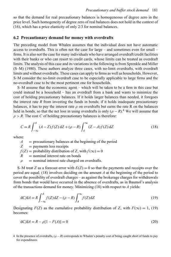
S–M assume that the economic agent – which will be taken to be a firm in this case butcould instead be a household – has an overdraft from a bank and wants to minimize thecost of holding precautionary balances. If it holds larger balances than needed, it foregoesthe interest rate R from investing the funds in bonds; if it holds inadequate precautionarybalances, it has to pay the interest rate ρ on overdrafts but earns the rate R on the balancesheld in bonds, so that the net loss in using overdrafts is only (ρ − R).4 We will assume thatρ > R. The cost C of holding precautionary balances is therefore:
C = R
∫ A
−∞(A − Z) f (Z) dZ + (ρ − R)
∫ ∞
A(Z − A) f (Z) dZ (18)
where:A = precautionary balances at the beginning of the periodZ = payments less receiptsf (Z) = probability distribution of Z , with f (∞) = 0R = nominal interest rate on bondsρ = nominal interest rate charged on overdrafts.
S–M treat Z as a forecast error with E(Z) = 0 so that the payments and receipts over theperiod are equal. (18) involves deciding on the amount A at the beginning of the period tocover the possibility of overdraft charges – as against the brokerage charges for withdrawalsfrom bonds that would have occurred in the absence of overdrafts, as in Baumol’s analysisof the transactions demand for money. Minimizing (18) with respect to A yields:
dC/dA = R
∫ A
−∞f (Z)dZ − (ρ − R)
∫ ∞
Af (Z)dZ (19)
Designating F(Z) as the cumulative probability distribution of Z , with F(∞) = 1, (19)becomes:
dC/dA = R −ρ[1 − F(A)] = 0 (20)
4 In the presence of overdrafts, (ρ −R) corresponds to Whalen’s penalty cost of being caught short of funds to payfor expenditures.

182 The demand for money
so that
F(A∗) = (ρ − R)/ρ (21)
where A∗ is the optimal value of A and F(A∗) is the cumulative probability that the optimalcash holdings will at least equal the need for cash.
To derive the optimal precautionary holdings, note that the precautionary balances willbe zero when actual overdrafts are positive. Therefore, the precautionary balances M pr
only equal:
M pr =∫ A∗
−∞(A∗ − Z) f (Z)dZ (22)
Assuming a normal distribution with zero mean:
M pr = A∗F(A∗) +σ f (A∗) (23)
where σ is the standard deviation of Z . In the case of a normal distribution, the averageamount borrowed through overdrafts (O) will be:
O = −A∗[1 − F(A∗)]+σ f (A∗) (24)
From (21) and (23),
∂M pr/∂ρ = [{1 − F(A∗)}
F(A∗)]/ρf (A∗) > 0 (25)
∂M pr/∂R = −F(A∗)/ρf (A∗) < 0 (26)
so that M pr decreases (and overdraft borrowings increase) when the bond rate R increasesand the overdraft rate ρ decreases. These are intuitively plausible results since a rise in R anda decrease in ρ increase the opportunity cost of holding precautionary balances.
There is no easy way to derive the interest elasticity of the precautionary money demand for(23) unless the probability distributions f (A) and F(A) are first specified. What is clear from(23) is that this demand depends upon these distributions and therefore upon their moments.Assuming a normal distribution, this demand will depend upon the mean and variance ofexpenditures, as in Section 6.1.
Equation (23) specifies the precautionary demand for money and does not include thetransactions demand. To compare the above analysis with that of Baumol’s transactionsdemand under certainty, now add the assumption of certainty to the present analysis. Theassumption for the uncertainty case was that E(Z) = 0. In the case of certainty, Z always has aknown value. If Z ≤ 0 (that is, receipts exceed payments every time), C in (18) would be zeroand so would be the demand for money derived from it. But if payments exceed receipts atdifferent points during the period, so that Z > 0, the individual will prefer to start with enoughtransactions balances in order to avoid using the more costly overdrafts with ρ > R. Hence,under certainty, the precautionary demand for money (exclusive of transactions demand) inthis analysis will be zero.

Precautionary and buffer stock demand 183
6.3 Precautionary demand for money without overdrafts
If the economic agent is not allowed overdrafts, the total cost consists of the interest lost onnot holding bonds and the cost of being overdrawn, which is assumed for the time being tobe equal to or less than the cost of having to postpone expenditures, so that:
C = R
∫ A
−∞(A − Z) f (Z) dZ +β
∫ ∞
Af (Z)dZ (27)
where β is the penalty to being overdrawn and the second integral on the right-hand sideis the probability of being overdrawn. Hence, the second term in (27) is the cost of beingoverdrawn. Minimizing (27) implies that:
F(A∗)/f (A∗) = β/R (28)
Since β is the penalty cost of holding inadequate balances, it can be compared with (ρ −R)in the analysis of Section 6.2, where ρ was the interest charged by the bank on overdraftbalances. In the present analysis, if the banks wanted to discourage some customers frombeing overdrawn they would set ρ and β fairly high, so that for such customers the operativevalue of β would become the penalty cost of finding funds elsewhere or of postponingexpenditures.
The response of M1 to the interest rate R, where R is the cost of holding M1, was derivedfrom (28) by S–M as:
∂M1pr/∂R = {F(A∗)2}/[R.f (A∗) −βf ′(A∗)] < 0 (29)5
where f ′ is the partial derivative of f with respect to A∗ and money is M1(which excludesthe assets on which the interest rate R is paid). The above analysis is very similar to that ofSection 6.2, with the penalty rate β corresponding to the overdraft interest charge ρ.
If money is defined very broadly as M3 to include the closest substitutes for M1, and Rs
is the interest rate on such substitutes, the S–M derivation showed that:
∂M3pr/∂Rs = [F(A∗){1 − F(A∗)
}]/[ρf (A∗) −βf ′(A∗)
]> 0 (30)
The difference in the signs of the partial derivatives in (29) and (30) occurs because R in(29) is the return on the alternative assets to M1 and therefore part of the cost of holding it,whereas Rs in (30) is the return on one of the (short-term) assets in M3.
The above two cases – with a no-limit overdraft and without an overdraft – illustrate thebasic nature of the S–M analysis; their analysis of the intermediate case of a binding limiton the overdraft is not presented here. The two analyses imply that, under uncertainty of thetiming of receipts and payments, there will be a positive precautionary demand for money.This demand has the general form:
M pr = M pr(R,ρ,β, f (z)) (31)
5 For the derivation of (28) and (29) from (27), see Sprenkle and Miller (1980, p. 417).

184 The demand for money
The elasticity of precautionary balances with respect to the bond rate R is negative.However, it is not possible to derive the interest and income elasticities of M1 and M2without further specification of the probability distribution of expenditures.6
6.4 Buffer stock models
The theoretical analysis of buffer stock models extends the inventory analysis of thetransactions demand for money to the case of uncertainty of net payments (payments lessreceipts), as in the case of the precautionary demand models of Sections 6.1 to 6.3. However,while this precautionary demand analysis has determined an optimal amount of precautionarybalances, the buffer stock models allow short-run money balances to fluctuate within a bandwhich has upper and lower limits, also known as thresholds, or fluctuate around a long-rundesired money demand.
There are basically two versions of buffer stock models. In one of these, a “policy decision”is made a priori by the individual that cash balances will be allowed to vary within anupper (Mmax) and a lower limit (Mmin). This case is depicted in Figure 6.1. When theautonomous – that is, independent of the decision to invest in bonds or disinvest from bonds –net receipts cause the accumulated cash balance to hit the upper limit Mmax, action is taken toinvest a certain amount in other assets, say bonds, thereby reducing cash holdings suddenlyby the corresponding amount. Whenever the autonomous net payments deplete the cashreserves sufficiently to reach the minimum permitted level Mmin, action is taken to rebuildthem by selling some of the bonds. This lower limit can be zero or a positive amount,depending upon institutional practices such as minimum balances required by banks, etc.Such buffer stock models with a pre-set band belong to the (Z , z) – with Z as the upperlimit and z as the lower one – type of inventory models and are called “rule models”,where the rule specifies the adjustment made when the money balances hit either of thelimits.
time
M
Mmax
Mmin
autonomouslump sumoutpayments
autonomouslump sum receipts
Investment inbonds
Figure 6.1
6 Sprenkle and Miller (1980) use some numerical examples to provide guidance on the money demand given bythe above analysis.

Precautionary and buffer stock demand 185
In such rule models, money balances can change because of positive or negative netpayments or because of action taken by the agent to reduce them when they reach theupper limit or increase them when they reach the lower limit. The former can be designatedas “autonomous” or “exogenous” changes and the latter as “induced” changes in moneybalances. In the former, the change occurs even though the agent’s objective is not to adjusthis money holdings. In the latter, the agent’s intention is to adjust the money balances sincethey have moved outside the designated band.
The second type of buffer stock models is called “smoothing or objective models.”In these, the objective is to smooth movements in other variables such as consumption orexpenditures and bond holdings. Unexpected increases in income receipts or decreases inpayments would be added to money balances acting as the “residual” inventory or temporaryabode of purchasing power until adjustments in expenditures and bond holdings can bemade. Conversely, unexpected decreases in income receipts or increases in payments wouldbe temporarily accommodated by running down money balances, rather than through animmediate cutback in expenditures or sales of bonds. The reason for thus treating moneyholdings as a residual repository of purchasing power is that the cost of small and continualadjustments in such balances is assumed to be lower than in either expenditures or payments,or in bond holdings, so that temporarily allowing such balances to change is the optimalstrategy. In such smoothing models, actual balances fluctuate around their desired long-rundemand, but there are no pre-set upper and lower limits as in the case of the rule models.This case is illustrated in Figure 6.2. Note that the distinction between the autonomousand induced (causes of) changes in money balances applies in both smoothing and rulemodels.
There can be quite a number of models of each variety. This chapter examines two modelsof each of the two versions of the buffer stock models. The models presented for the ruleversion are those by Akerlof and Milbourne (A–M) (1980) and Miller and Orr (M–O) (1966).The models presented for the smoothing version are those of Cuthbertson and Taylor (C–T)(1987) and Kanniainen and Tarkka (K–T) (1986).
long rundesired balances
M
time
actualbalances
Figure 6.2

186 The demand for money
6.5 Buffer stock rule models
6.5.1 The rule model of Akerlof and Milbourne
We start the analysis of buffer stock models with the contribution of Akerlof and Milbourne(A–M) (1980). As in Baumol’s transactions demand model, A–M7 assume a lump-sumreceipt of Y at the beginning of the period and expenditures of C at a constant rate throughthe period. However, in a departure from Baumol’s model, A–M assume that C ≤ Y , withsaving S = Y − C. Saving during the period is added to money balances until the latterreach the set upper limit, at which time action is taken to decrease them to C throughtheir partial investment in bonds, so that they are expected to be exhausted by the nextperiod.
Designate the upper limit as Z and the lower one as z, with the latter taken to be zerofor simplification. The agent wishes to start each period with the amount C, which willtherefore be the desired amount at the beginning of each period. The actual amounts held atthe beginning of the ith period equal C + iS, as long as (C + iS) ≤ Z . If the upper limit isreached after n periods, we have:
C + nS ≥ Z ≥ C + (n − 1)S (32)
so that:
n ≥ (Z − C)/S ≥ (n − 1) (33)
Hence, the maximum and minimum values of n are:
nmax = [(Z − C)/S]+ 1 (34)
nmin = [(Z − C)/S] (35)
The amount C is spent evenly during the period so that the average amount of cashbalances corresponding to it is C/2. When saving S is added to money balances in a period,this amount is held from the beginning of the period to its end, so that the average cashbalances corresponding to it are S. Therefore, the sequence of money balances at the end ofeach period is:
{C/2,C/2 + S,C/2 + 2S, . . .,C/2 + (n − 1)S
}(36)
which equals:
(C/2){1,1 + S,1 + 2S, . . . ,1 + (n − 1)S
}
7 The model presented below is only the basic one from Akerlof and Milbourne. For its more complex forms andfor numerical illustrations, see the original article.

Precautionary and buffer stock demand 187
Let n be the number of periods before an induced transfer takes place. Then, over n periods,the average balance between induced adjustments is:
M d = 1
n
[C
2+(
C
2+ S
)+(
C
2+ 2S
)+·· ·+
{C
2+ (n − 1)S
}]
= C
2+ S(n − 1)
2(37)
Using (34) and (35) to eliminate n in (37) implies the minimum and maximum values ofmoney balances as:
Mmax = Z/2 (38)
Mmin = (Z − S)/2 (39)
Hence, the average of the money balances held as a buffer stock, designated as M b, is:
M b = (1/2)(Mmax + Mmin)
= Z/2 − S/4(40)
so that:
∂M b/∂Y ∼= −(1/4)(∂S/∂Y ) < 0 (41)
where ∂S/∂Y is the marginal propensity to save, which is positive. Hence, ∂M b/∂Y isnegative. This is a surprising result. Its intuitive explanation is that, as income rises, theupper threshold is reached more quickly, so that the interval before the money holdings arerun down by an induced adjustment is shortened. As a result, the richer agents review theirmoney and bond holdings more often than those with lower incomes, ceteris paribus, andwill hold less balances on average.8
However, since the limits z and Z were assumed to be exogenously specified in theabove model, the impact of increases in Y on them is not incorporated in (40). Transactionsdemand analysis implies that both of these limits would be positive functions of the level ofexpenditures.9 Therefore, the impact of a rise in income would have a positive and a negativecomponent, with the net impact being of indeterminate sign unless a fuller model werespecified. Another limitation of the above model is that it does not distinguish between theexpected increases in income and the unexpected ones. The (z, Z) concept is more appropriateto the latter than to the former.
Akerlof and Milbourne extended their preceding model to the case of the uncertainty ofnet payments by assuming that the agent buys and pays for durable goods at uncertain times,with p as the probability of making such a purchase. For this case, the A–M result, under their
8 This result does not hold if the upper limit X is defined relative to income Y as xY.9 If we follow the pattern of Baumol’s transactions analysis, suitably adapted to the present context, z and Z will
be non-linear functions of Y .

188 The demand for money
simplifying assumptions that include S = sY , where s is the constant average propensity tosave, was that:
M b ≈ Z/2 − s (1 + p)(Y/4) < 0 (42)
where p is the probability of payments (for a durable goods purchase). (42) implies that:
∂M b/∂Y = −(s/4)[1 + p + Yp′(Y )] (43)
where p′ = ∂p/∂Y . Assuming p′ to be positive – that is, the probability of buying durablegoods increases with income – (43) implies that the income elasticity of money balances isagain negative.
The A–M model was meant to encompass both the transactions and precautionary demands.The agent’s desire to finance an amount of transactions C out of income receipts Y createshis transactions demand, while the uncertainty of payments adds an additional precautionarydemand. However, this framework does not properly capture the transactions demand since itignores the dependence of (z, Z) on total expenditures and does not make a distinction betweenexpected and unexpected changes in income. Its implication of a negative income elasticity ofmoney demand must therefore be accepted as reflecting the influence of saving, and especiallyunexpected saving, on money demand, with consumption – and hence permanent income –being held constant. Some of the ideas behind these criticisms will become clearer from thetheoretical and empirical models presented below.
6.5.2 The rule model of Miller and Orr
Miller and Orr (M–O) (1966) assumed that net receipts – which would be net payments for anegative value – of x at any moment follow a random walk with a zero mean over each period(e.g. a “day”).10 Assume that in any time interval (e.g. an “hour”) equaling 1/t(t = 24), xis generated as a sequence of independent Bernoulli trials. The individual believes with asubjective probability of p that he will have net receipts of x during each time interval (hour)or net payments of x with a probability of (1−p), so that, over an hour, the probability of anincrease in money holdings by x is p and that of a decrease by x is (1 − p).
Cash holdings over a decision period of T periods will have a mean and standard deviationgiven by:
μT = Ttx (p − q) (44)
σ 2T = 4Ttpqx2 (45)
where:x = net receipts per hourμT = mean cash holdings over T periodsσT = standard deviation of cash holdings over T periodsp = probability of positive net paymentsq = probability of negative net payments (= 1 − p)t = number of sub-intervals (hours) in each period (day)T = number of time periods up to the planning horizon.
10 Under this assumption, the pattern of net payments will possess stationarity and serial independence.
Precautionary and buffer stock demand 189
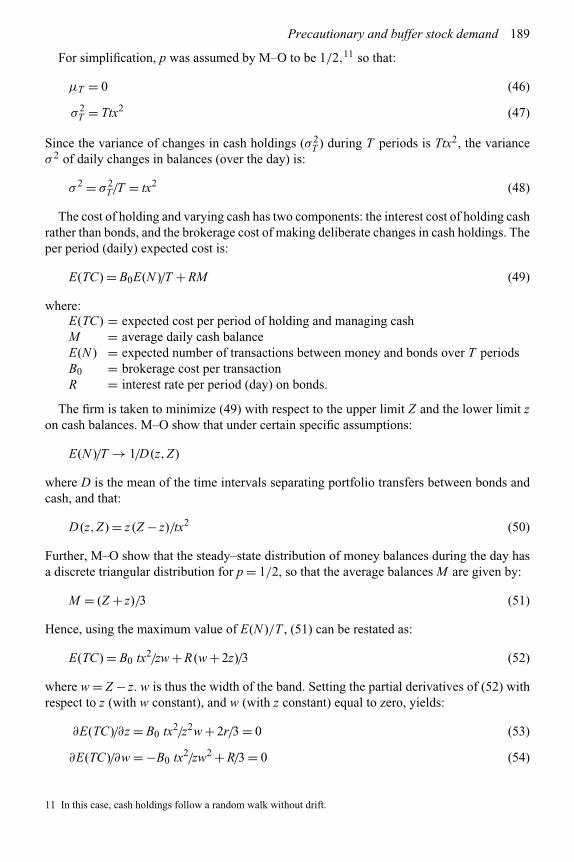
For simplification, p was assumed by M–O to be 1/2,11 so that:
μT = 0 (46)
σ 2T = Ttx2 (47)
Since the variance of changes in cash holdings (σ 2T ) during T periods is Ttx2, the variance
σ 2 of daily changes in balances (over the day) is:
σ 2 = σ 2T/T = tx2 (48)
The cost of holding and varying cash has two components: the interest cost of holding cashrather than bonds, and the brokerage cost of making deliberate changes in cash holdings. Theper period (daily) expected cost is:
E(TC) = B0E(N )/T + RM (49)
where:E(TC) = expected cost per period of holding and managing cashM = average daily cash balanceE(N ) = expected number of transactions between money and bonds over T periodsB0 = brokerage cost per transactionR = interest rate per period (day) on bonds.
The firm is taken to minimize (49) with respect to the upper limit Z and the lower limit zon cash balances. M–O show that under certain specific assumptions:
E(N )/T → 1/D (z,Z)
where D is the mean of the time intervals separating portfolio transfers between bonds andcash, and that:
D (z,Z) = z (Z − z)/tx2 (50)
Further, M–O show that the steady–state distribution of money balances during the day hasa discrete triangular distribution for p = 1/2, so that the average balances M are given by:
M = (Z + z)/3 (51)
Hence, using the maximum value of E(N )/T , (51) can be restated as:
E(TC) = B0 tx2/zw + R (w + 2z)/3 (52)
where w = Z − z. w is thus the width of the band. Setting the partial derivatives of (52) withrespect to z (with w constant), and w (with z constant) equal to zero, yields:
∂E(TC)/∂z = B0 tx2/z2w + 2r/3 = 0 (53)
∂E(TC)/∂w = −B0 tx2/zw2 + R/3 = 0 (54)
11 In this case, cash holdings follow a random walk without drift.

190 The demand for money
which yield the optimal values z∗ and w∗ as:
z∗ = (3B0 tx2/4R)1/3 (55)
w∗ = 2z∗ (56)
Since w = Z − z, (56) implies that the optimal upper limit Z∗ will be:
Z∗ = 3z∗ (57)
Equation (57) specifies the relative width of the band between the upper and lower limits as:
(Z − z)/z = 2
which is independent of the interest rate and the brokerage cost, though, by (55) to (57), theabsolute width of the band does depend upon these variables.
From (57), the mean buffer stock balances M b under the assumptions of this model aregiven by:
M b = (Z + z)/3 (58)
Therefore, the average optimal buffer stock balances M b∗ derived from (55), (57) and(58) are:
M b∗ = 4
3
(3B0 t x2
4R
)1/3
= 4
3
(3B0 σ 2
4R
)1/3
(59)
since σ 2 = tx2. In (59), the average demand for money depends upon the interest rate andthe brokerage cost, as in the certainty version of the transactions demand analysis, and uponthe variance of net payments, as in the precautionary demand analysis. The elasticity of theaverage demand for money with respect to the variance of income is 1/3, and with respect tointerest rates it is (−1/3), as in Whalen’s (1966) analysis.
However, M–O pointed out that, since there does not exist a precise relationship betweenσ 2 and Y , there will not exist a precise income elasticity of M b with respect to Y . Toillustrate, if we are dealing with a firm’s demand for money and Y is its income from sales,a proportionate increase in this sales income due to a proportionate increase in all receiptsand payments by it, with their frequency unchanged, will increase x proportionately, so thatσ 2 = tY 2, implying from (59) an income elasticity of 2/3, as in Whalen. But if the amount ofeach receipt and payment does not change but their frequency is increased, so that t increasesproportionately with Y such that t = αY , we have σ 2 = αYx2, thereby implying from (59)an income elasticity of 1/3, again as in Whalen. The implied range for the income elasticityof the average buffer stock balances becomes even larger than from 1/3 to 2/3 if the amountsof the transactions increase while their frequency decreases.
The M–O model extends the analysis of the precautionary demand for money to the casewhere there are fluctuations within upper and lower limits, with these limits derived in anoptimizing framework. The existence of a range for the income elasticity of the average bufferstock balances, rather than a single value as for Baumol’s transactions balances, is anotherempirically appealing feature of the M–O model. These authors considered their model to beespecially appealing in explaining the firms’ demand for money.

Precautionary and buffer stock demand 191
6.6 Buffer stock smoothing or objective models
6.6.1 The smoothing model of Cuthbertson and Taylor
The basic partial adjustment model (PAM), in the context of a single period, often assumesthat the adjustment in money balances involves two kinds of costs. One of these is the costof deviations of actual balances from their desired amount. The second element is the costof changing the current level of balances from their amount in the preceding period. Theone-period first-order PAM12 assumes that the cost function is quadratic in its two elements,as in:
TC = a (Mt − M ∗t )2 + b (Mt − Mt−1)2 (60)
where:TC = present discounted value of the total cost of adjusting balancesM = actual money balancesM ∗ = desired money balances.
The buffer stock models (Carr and Darby, 1981; Cuthbertson, 1985; Cuthbertson andTaylor, 1987; and others) posit an intertemporal cost function rather than a one-period oneand minimize the present expected value of this cost over the present and future periods.This implies taking account of both types of costs over the present as well as the futureperiods. Hence, for the first element of cost, the expected cost of future deviations of actualfrom desired balances, in addition to the cost of a current deviation, is taken into account.This modification allows the agent to take account of the future levels of desired balances indetermining the present amounts held. For the second element of cost, the justification forthe intertemporal extension is as follows: just as last period’s money holdings affect the costof adjusting this period’s money balances, so would this period’s balances affect the cost ofadjusting next period’s balances, and so on, and these future costs attached to current moneybalances need to be taken into consideration in the current period. The resulting cost functionis intertemporal and forward looking.
The intertemporal extension of (60) for i = 0,1, . . .,T is:
TC = �iDi[a(Mt+i − M ∗
t+i)2 + b(Mt+i − Mt+i−1)2
](61)
where:
D = gross discount rate (= 1/(1 + r)).
In equation (61), a is the cost of actual balances being different from desired balances andb is the cost of adjusting balances between periods. b can be the brokerage cost of sellingbonds but, as we have seen in earlier discussions, this can be more than just a monetary cost.The economic agent is assumed to minimize TC with respect to Mt+i, i = 0,1, . . . ,T . ItsEuler condition for the last period T is:
∂TC/∂Mt+T = 2a(Mt+T − M ∗t+T ) + 2b(Mt+T − Mt+T−1) = 0
12 See Chapter 7 for the treatment of one-period partial adjustment models in the context of money demandfunctions.

192 The demand for money
so that:
Mt+T = a
a + bM ∗
t+T + b
a + bMt+T−1
= A1M ∗t+T + B1Mt+T−1
(62)
Where A1/(a+b) and A1 +B1 = 1. For i < T , the first-order cost-minimizing conditions are:
∂C
∂Mt+i= 2a (Mt+i − M ∗
t+i) + 2b (Mt+i − Mt+i−1) − 2b (Mt+i+1 − Mt+i) = 0
Mt+i = a
a + 2bM ∗
t+i +b
a + 2bMt+i−1 + b
a + 2bMt+i+1
= A2M ∗t+i + B2Mt+i−1 + B2Mt+i+1
(63)
where A2 +2B2 = 1. In (63), both the future and past values of actual balances M , as well asthe future values of M ∗, affect the demand for money in each period. (63) implies13 that:
Mt = q1Mt+i−1 + (a/b)q1 �iqiiM
∗t+i (64)
where q1 + q2 = (a/b) + 2 and q1q2 = 1. We need to specify the demand function for thedesired money balances M ∗. As derived in Chapters 2 and 3, assume it to be:
M ∗t+i/pt+i = byyt+i + bRRt+i (65)
Further, in the context of uncertainty and using the expectations operator Et−1 for expectationsheld in t−1, let:
Mt = Et−1Mt + Mut +μt (66)
13 For the derivation, see Cuthbertson (1985, pp. 137–8; Cuthbertson and Taylor, 1987, pp. 187–8). The followingderivation is from Cuthbertson (1985, pp. 137–8). The steps are:Multiply (63) by (a + 2b) and rearrange to:
(a + 2b − bL − bL−1)M = aM ∗
where L−1 is the forward (as opposed to the lag) operator, so that L−1Mt = Mt−1. Multiply by L and divide bothsides by b. This gives:[
−L
(a + 2b
b
)+ L2 + 1
]M = − a
bM ∗−1
[−L
(a + 2b
b
)+ L2 + 1
]= (1 − q1L)(1 − q2L)
= 1 − (q1 + q2)L + q1q2L2
where q1 + q2 = (a/b) + 2 and q1q2 = 1. Assume q2 > 1, so that q1 < 1. Hence,
(1 − q1L)M = (1a/b)(1 − q2L)−1M ∗−1
= (−a/b)(1 − q−11 L)−1M ∗−1
Using the Taylor expansion, (1 − lL)−1 = −(lL)−1 − (lL)−2 −·· · , we get:
Mt = q1Mt−i−1 + (a/b)q1 �i qiiM
∗t+i

Precautionary and buffer stock demand 193
where M ut has been introduced to take account of errors in the expected value of M ∗
t+i due tounexpected changes in its determinants in (65). From (64) to (66),
Mt = q1Mt−1 + (a/b)q1�i qii
{byyt+i + bRRt+i
}pt + M u
t +μt (67)
In (67), the actual demand for money depends upon the future and current values of incomeand interest rates, which shows the model to be a forward-looking one. It also depends uponthe lagged value of money balances, thus incorporating a backward-looking element. Themodel is, therefore, both forward and backward looking. Note that the estimation of (67)will require the prior specification of the mechanism for deriving the expected future valuesof y and R, and also of the mechanism for the estimation of M u. The estimation proceduresfor these are discussed in Chapter 7.
6.6.2 The Kanniainen and Tarkka (1986) smoothing model
An alternative version of the intertemporal adjustment cost function (61), used by Kanniainenand Tarkka (K–T) (1986),14 is:
TC = Et�i[Di{a(Mt+i − M ∗
t+i)2 + b (zt+i)
2}] i = 0,1,2, . . . (68)
where zt are the “induced” changes in money balances brought about by the agent’s ownactions and b is interpreted as the brokerage cost of converting bonds to money. The othervariables are as defined earlier, with M being nominal balances, M ∗ the steady-state desiredbalances and D the discount factor. The rationale for this specification of the cost function isthat while the induced changes in money holdings impose a brokerage cost, the autonomouschanges do not since they result from the actions of others. The adjustment in nominalbalances in t from those in t−1 occurs due to autonomous and induced changes in t, so that:
Mt − Mt−1 = zt + xt (69)
where:zt = induced changes in money holdingsxt = autonomous changes.
Substitute (69) in (68) and, to minimize total cost, set the first-order partial derivatives ofthe resulting equation with respect to mt+i, i = 0,1,2, . . ., equal to zero. This process yieldsthe Euler equations as:
EtMt+i+1 −βEtMt+i + (1 + R)EtMt+i−1 = −αEtM∗t+i + Etxt+i+1 − (1 + R)Etxt+i
(70)
where:α = a/Dbβ = (1/D)
{(a/b) + D + 1
}i = 0,1,2, . . . .
Note that (70) represents a large number of equations and shows the extensive informationrequirements of such models. To determine money demand in period t, the agent must have
14 The following exposition is based on Kanniainen and Tarkka (1986) and Mizen (1994, pp. 50–51).

194 The demand for money
expectations on the autonomous changes in money holdings in (t +1) and its optimal moneybalances, with the latter requiring this information for period (t + 2), and so on. With newinformation becoming available each period, the model will require continual recalculation.
Equation (70) is a stochastic second-order difference equation in Et Mt+i. Its roots are:
l1,l2 = (1/2)[β ± {β2 − 4(1 + R)
}1/2]
with l1 > 0 being the stable root and l2 < 0 being the unstable one. The latter was ignored byK–T in order to exclude cyclical adjustment. Using the positive root l1, the Euler conditionbecomes:
EtMt+1 = l1Mt +[l1α/(1 + R − l1)
]M ∗
t −�i[l1/(1 + R)
]i[Etxt+i−1 − (1 + R)Etxt+i
](71)
In (71), the impact of the autonomous adjustment xt on money demand is given by l1, thestable root of (70). This impact is the same whether it was anticipated or not.15 The impact offuture autonomous shocks, on which expectations have to be formed, depends upon the rateof time preference. If this rate is high, these expectations will have to be formed for only someperiods ahead. Further, changes in these expectations will shift the money demand function.
Substitute (71) into (70) and solve for Mt , noting that EtM ∗t = M ∗
t . This yields:
Mt = l1Mt−1 +ρM ∗t + l1xt + zt (72)
where ρ = [l1(a/b)(1 + R)/
(1 + R − l1)] and z∗t represents the weighted sum of the future
shocks to net receipts and payments. z∗t is given by:
z∗t = −(1 − l1)�i
{l1/(1 + R)
}iEtxt+j (73)
The above model can be transformed into real terms by dividing (71) by the current pricelevel pt . The resulting equation, based on (71),16 is:
ln mt = a0 + (1 − l1)ln m∗t + l1ln mt−1 + γ ln pt/pt−1 + l1xt/Mt−1 + zt/Mt−1 (74)
where mt = Mt/Pt and m∗t = M ∗
t /Pt .
15 This conclusion differs from that of Carr and Darby (1981) and Santomero and Seater (1981).16 The procedure is as follows. Subtracting Mt−1 from both sides of (72) gives:
Mt − Mt−1 = (1 − l1)[ρ/(1 − l1)M ∗
t − Mt−1]+ l1xt + zt
Divide both sides of this equation by Mt−1 and use the approximation ln (1+n) ∼= n for small values of n. Thisgives:
In Mt = ln[ρ/(1 − l1)
]1−l1 + (1 − l1)ln M ∗t + l1Mt−1 + l1xt/Mt−1 + zt/Mt−1
Now subtract ln pt from both sides and also add and subtract the term l1 ln pt−1. This will give (74) with
a0 = ln[ρ/(1 − l1)
]1−l1 . See K–T for the derivations of these equations and those reported in the text.

Precautionary and buffer stock demand 195
K–T specified the desired demand m∗t as a log-linear function of yt and Rt , such that:
m∗t = γ yθ
t Rηt (75)
Where θ and η are parameters. The critical autonomous net payments variable xt wasdefined as:
xt = �Lt +�Lgt + Bt (76)
where:L = domestic credit expansionLg = government net borrowing from abroadB = surplus in the balance of payments on current account
On the future values of xt , the following extrapolative model was assumed:
Etxt+i = xt(1 + θ )i
where θ can be positive or negative or zero. Assuming zt+i to be proportional to xt+i suchthat Zt+i = −ξXt+i, K–T use (74) to specify the estimating equation as:
ln mt = a0 + (1 − l1) ln m∗t + l1ln mt−1 + γ ln pt/pt−1 + (l1 − ξ ) xt/Mt−1 +μt (77)
where μ is random noise. Note that the current autonomous injections of money increasecurrent money holdings through the variable xt .
The differences between (67), which is the estimating equation for Cuthbertson and Taylor,and (77), which is the estimating equation for K–T, arise from their different cost functions.(77) is derived from (68), which assumes that only induced changes in money balances imposeadjustment costs, whereas (67) is derived from (61), which attaches such costs to the totaldifference between balances in periods t + i and t + i−1 and, as such, requires a wider notionof adjustment costs than merely brokerage costs. Both models are forward (and backward)looking models and require specification of the procedures for estimating the future valuesof the relevant variables. They also require specification of the estimation procedure for netpayments and receipts. Part of these net payments and receipts can be anticipated and partunanticipated.
The two approaches of Cuthbertson et al and of Kanniainen and Tarkka are similar inmany ways. Both are examples of smoothing buffer stock models in which money holdingsare free to vary from their desired levels. Such models illustrate some of the most commonelements used for specifying the buffer stock analysis of the demand for money. Their criticalfeature is that the autonomous injections of money supply in the economy are, for some time,passively absorbed by the public in actual money holdings.
To give an indication at this stage of the empirical findings on the critical points in the aboveanalysis, we here briefly mention Kanniainen and Tarkka’s empirical results. They estimatedtheir model for five industrialized economies (West Germany, Australia, USA, Finland andSweden) for the period 1960–82. The estimated coefficients of their model had the predictedsigns and plausible magnitudes. The lagged money variable had a magnitude consistent withother studies. However, as indicated by their estimate of γ , the adjustment of money balancesto changes in prices was found to be costly. Their buffer stock equation performed betterthan the standard (non-buffer stock) money demand models: the coefficients of the injection

196 The demand for money
variable xt+i were positive and significant, thus supporting the buffer stock approach. Thesefindings also support the hypothesis that the monetary injections from different sources arefirst absorbed in nominal money holdings and then dissipated.
6.7 Empirical studies on the precautionary and buffer stock models
While the transactions, speculative and precautionary models determined a unique optimaldemand for money for each component, the buffer stock models allowed fluctuations inmoney holdings either in a band or around an optimal long-run path. These models areforward (and backward) looking and require specification of the procedures for estimatingthe future values of the relevant variables. They also require specification of the estimationprocedure for net payments and receipts. Part of these net payments and receipts can beanticipated and part unanticipated. Another feature of the buffer stock models for estimationpurposes is that the unanticipated injections of money supply in the economy are, for sometime, passively absorbed by the public.
There are two broad types of empirical studies of the buffer stock money demand. One ofthese distinguishes between a long-run (planned or permanent) desired money demand anda short-run (buffer stock or transitory) money demand, and estimates their sum by standardregression techniques. The empirical works of Darby (1972), Carr and Darby (1981) andSantomero and Seater (1981), among others, belong in this category. We shall refer tothis category as the shock-absorption money-demand models. The second type of empiricalstudies uses cointegration techniques and error-correction modeling. Since these techniqueswill be discussed in Chapter 8, which also reports on their findings on money demand, thischapter reports on only the former type of studies.
Shock-absorption money demand models
Darby (1972) proposed and tested a version of the “shock-absorption” model of moneydemand. In setting up his model, he argued that most of any positive transitory saving will beinitially added to money balances and then gradually reallocated to other assets or be depletedby subsequent negative transitory saving – with money balances reverting to their long-rundesired (“permanent”) levels at the end of these adjustments. Money balances therefore, actto absorb shocks in income and saving. The Darby shock-absorber model is an early versionof the buffer stock models of money and limits its shocks to innovations in income.
Darby separated money holdings into two categories, permanent and transitory, as in:
Mt = MPt + MT
t (78)
The demand for permanent money balances was assumed by Darby to be:
MPt = α0 +αyY P
t +αRLRLt +αRSRSt +αRM RMt (79)
where:MP = permanent real balancesMT = transitory real balancesY P = permanent real incomeY T = transitory real incomeRL = long-term nominal interest ratesRS = short-term nominal interest rateRM = nominal yield on money balances.

Precautionary and buffer stock demand 197
Equation (79) specifies the dependence of permanent balances on permanent income andvarious interest rates.
For transitory balances MT, Darby assumed that:
�MTt = β1ST
t +β2MTt−1 0 > β1 > 0, β2 < 0 (80)
where the proportion β1 of transitory real saving ST is added to transitory real balances duringthe period, but last period’s transitory balances are run down or adjusted at the rate β2.
Darby used Milton Friedman’s ideas on permanent and transitory income in which:
Yt = Y Pt + Y T
t (81)
where permanent and transitory income are not correlated with each other and permanentincome is generated by an adaptive expectations procedure. Further,
STt = Y T
t − CTt (82)
where transitory consumption CT is an independent random variable with a zero mean, so thatY T
t was substituted for STt in the estimating equation. As mentioned above, a proportion β1 of
it is accumulated in transitory money balances during the period and eventually reallocatedto other assets.
Equations (78) to (82) imply that:
Mt = α0 (1 −β) +β1Y Tt +βMt−1 +αY Y P∗
t +αRLRL∗t +αRSRS∗
t +αRM RM ∗t (83)
where β = (1 + β2), Y P∗ = (1 − β)Y Pt , RL∗
t = (1 − β)RLt, RS∗t = (1 − β)RSt and
RM ∗t = (1 −β)RMt .
Darby’s finding for USA for the period 1947:1 to 1966:4 was that β1 was about 40 percent,so that transitory income and saving had a strong effect on money balances and transitorybalances increased by about 40 percent of transitory income. β2, the induced reduction intransitory balances per quarter, was about 20 percent. These findings support the bufferstock approach where net income receipts are temporarily added to money balances and thengradually adjusted at periodic intervals. The estimated adjustment is relatively slow, thoughDarby also found that both β1 and β2 had increased since the 1940s. With the increasinginnovation in the financial markets in recent decades, the increase is likely to have continuedand be quite significant.
While the above model introduces the notion of transitory money balances arising fromtransitory income and saving into the analysis, it does not deal with the differing effects ofanticipated and unanticipated changes in the money supply, and therefore does not deal withinnovations in money supply. Carr and Darby (1981) argue that the anticipated changes inmoney supply are integrated by economic agents into their decisions on consumption, etc. andare therefore already incorporated into the current price level, with real balances held beingunaffected by the changes in the price level and the anticipated money changes. However,the unanticipated money supply change alters the net receipts of the public and can be treatedas an element of transitory income. It may be wholly or partly added to buffer balances, isthereby not spent and is not reflected in the price level. Hence, changes in the unanticipatedmoney supply alter real balances while changes in the anticipated money supply do not.

198 The demand for money
To incorporate these arguments into the analysis, Carr and Darby (1981) assumed that:
M st = M s∗
t + M sut (84)
where:M s = nominal money supplyM s∗ = anticipated nominal money supplyM su = M s − M s∗ = unanticipated nominal money supply.
The short-run desired demand function was specified in real terms, with a partial adjustmentmodel, as:
mdt − mt−1 = l (m∗
t − mt−1) (85)
where:md = short-run desired demand for real balances (log scale)m* = long-run desired demand for real balances (log scale)
so that the desired short-run demand for real balances is:
mdt = lm∗
t + (1 − l)mt−1 (86)
where the short-run desired demand for real balances is a weighted average of the long-rundemand and one-period lagged balances. The actual holdings of money balances are the sumof the short-run desired balances, transitory income and unanticipated money supply. Hence:
mt = lm∗t + (1 − l)mt−1 +βyT
t + bM sut (87)
The long-run desired demand is given by:
m∗t = γ0 + γ1yP
t + γ2Rt (88)
Therefore:
mt = lγ0 + lγ1yPt + lγ2Rt + (1 − l)mt−1 +βyT
t + bM sut (89)
Permanent and transitory income were measured as in the Darby model earlier; incalculating permanent income, the weight on the current quarterly income was set at0.025 percent. In the present model, the demand for real balances depends upon transitoryincome and unanticipated money supply changes. The theoretical arguments require theircoefficients to be positive.
Carr and Darby (1981) tested this model for eight industrial countries (USA, UK, Canada,France, Germany, Italy, Japan and the Netherlands) for the period 1957:1 to 1976:4 andreported that the coefficient b on unanticipated money supply was significant and rangedbetween 0.7 and 1 for all countries, using generalized least-squares (GLS) estimates. Thecoefficient β was significant and positive for the USA but was not significant for the othercountries. To illustrate, using GLS estimates for the coefficients, the estimated value of β (thecoefficient for transitory income) was 0.090 while that of b (the coefficient for unanticipatedmoney supply) was 0.803 for the USA; the corresponding estimate of β for Canada was0.018, which was not significant, but the estimate of b was 0.922 which was significant.Hence, the influence of transitory income on money balances was much weaker than that
Precautionary and buffer stock demand 199
of unanticipated money supply changes, with most of the latter added to money balances inthe current quarter, so that the impact effect of such changes on the price level or economicactivity would be minimal.
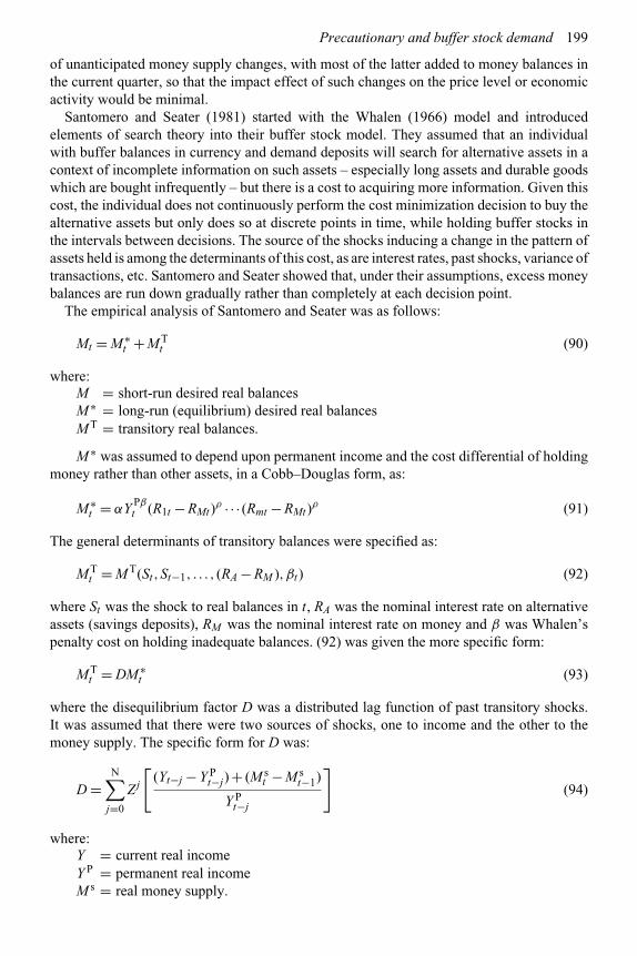
Santomero and Seater (1981) started with the Whalen (1966) model and introducedelements of search theory into their buffer stock model. They assumed that an individualwith buffer balances in currency and demand deposits will search for alternative assets in acontext of incomplete information on such assets – especially long assets and durable goodswhich are bought infrequently – but there is a cost to acquiring more information. Given thiscost, the individual does not continuously perform the cost minimization decision to buy thealternative assets but only does so at discrete points in time, while holding buffer stocks inthe intervals between decisions. The source of the shocks inducing a change in the pattern ofassets held is among the determinants of this cost, as are interest rates, past shocks, variance oftransactions, etc. Santomero and Seater showed that, under their assumptions, excess moneybalances are run down gradually rather than completely at each decision point.
The empirical analysis of Santomero and Seater was as follows:
Mt = M ∗t + MT
t (90)
where:M = short-run desired real balancesM ∗ = long-run (equilibrium) desired real balancesMT = transitory real balances.
M ∗ was assumed to depend upon permanent income and the cost differential of holdingmoney rather than other assets, in a Cobb–Douglas form, as:
M ∗t = αY Pβ
t (R1t − RMt)ρ · · · (Rmt − RMt)
ρ (91)
The general determinants of transitory balances were specified as:
MTt = MT(St,St−1, . . . , (RA − RM ),βt) (92)
where St was the shock to real balances in t, RA was the nominal interest rate on alternativeassets (savings deposits), RM was the nominal interest rate on money and β was Whalen’spenalty cost on holding inadequate balances. (92) was given the more specific form:
MTt = DM ∗
t (93)
where the disequilibrium factor D was a distributed lag function of past transitory shocks.It was assumed that there were two sources of shocks, one to income and the other to themoney supply. The specific form for D was:
D =N∑
j=0
Zj
[(Yt−j − Y P
t−j) + (M st − M s
t−1)
Y Pt−j
](94)
where:Y = current real incomeY P = permanent real incomeM s = real money supply.

200 The demand for money
Equation (94) assumes that all shocks, whether from income or money supply changes,have the same pattern of effects on transitory balances. Further, innovations in money demandare not considered, so that either they do not occur17 or real balances adjust instantly to them.If the money demand function is unstable, (94) should be modified to include shifts in moneydemand.
The estimated demand function for short-run balances implied by (90) to (94) is of theform:
M dt = αY
Pβt (R1t −RMt )γ · · · (Rmt −RMt )ρ
×⎡⎣1 +
N∑j=0
Zj
((Yt−j −Y P
t−j) + (M st −M s
t−1
Y Pt−j
)⎤⎦
δ
(95)
where α,β,δ > 0 and γ,ρ < 0, and Ri is the nominal rate of return on the ith asset.The above model was estimated for M1 and M2 for the USA for the period 1952:2 to
1972:4, using the Cochrane–Orcutt technique to eliminate first-order serial correlation. Itwas assumed in the estimation process that equilibrium was achieved within each quarterbetween the money supply and the short-run money demand, so that the latter was proxied bythe money supply. Only two interest rates – the commercial paper rate and the commercialpassbook rate – were used. The estimate of the coefficient Z was significant and positivefor both M1 and M2. Hence, both transitory income and changes in the money supply had ashort-run positive impact on short-run money demand, thereby showing evidence of bufferholdings of money balances. Further, transitory balances did not increase proportionatelywith the magnitude of the shock, so that large shocks were corrected faster than smaller ones.M1 and M2 holdings adjusted within two to three quarters to their desired levels, implyinga fairly fast rate of adjustment.
A microfoundations search model of precautionary balances
Faig and Jerez (2007) use microeconomic optimizing foundations to model the demand formoney as a demand for precautionary balances held against uncertain expenditure needs.They build a search model incorporating shocks to individuals’ preferences. Individualsdecide on their money balances prior to the unknown preference shock, with large preferenceshocks assumed to be rarer than small ones. At low interest rates, individuals hold enoughbalances so that their consumption purchases are not very liquidity constrained, but theyare willing to allow their purchases to be liquidity constrained to a greater extent at higherinterest rates, so that velocity falls at higher interest rates. Their empirical estimates forthe USA for the periods 1892 to 2004 capture the fall in the velocity of M1 during thelow-interest period of the Great Depression and its rise from the mid-1960s to the mid-1980s, which had high interest rates. Financial innovations, such as credit cards, Internetbanking, etc., as well as the reduction in brokerage costs (which has reduced the cost oftransfers between M1 and other assets), have meant that households can better accommodateunexpected expenditures, even with inadequate money balances. These developments have
17 Santomero and Seater (1981) assume that the money demand function is stable. In fact, empirical studies inrecent decades have shown it to be unstable and therefore to generate transitory excess money holdings.

Precautionary and buffer stock demand 201
reduced the need for precautionary balances. Therefore, the empirical impact of financialinnovations and the IT revolution has been to reduce the demand for M1 and increase itsvelocity.
Conclusions
This chapter has presented some of the basic models of the precautionary demand for money.This demand arises because of the uncertainty of the timing of payments and receipts, so that amajor determinant of such demand is the probability distribution of net payments. Whalen’sanalysis captured this by the variance of the distribution, under the assumptions that thedistribution was normal and the individual wanted to keep balances equal to a specifiedproportion of the variance of the distribution. How much of this proportion is kept by aparticular individual will depend upon his degree of risk aversion. This analysis shows thatthe elasticities of precautionary demand with respect to interest rates and income are not 1/2,as were the elasticities for transactions demand under certainty of the timing of receipts andpayments, but are likely to be lower.
The precautionary demand analysis also brings the interest rates on stand-by credit facilitiessuch as overdrafts and trade credit, and the penalties for being caught short of a paymentmedium, into the determinants of the precautionary demand and through it into those of thetotal demand for money. Such facilities and penalties differ between households and firms,and between large and small firms. Further, they often also differ by industry, so that weshould expect the demand functions for money to differ between sectors and industries.
Is the precautionary demand for money a significant part of the total money balances?The answer to this will depend upon the degree of uncertainty of income and expenditures,and the relative penalty costs of being caught short of funds. Some numerical calculationsdone by Sprenkle and Miller suggest that the precautionary balances can be about one-thirdor more of the transactions balances. Further, with the increasing availability of short-termassets, which offer a higher return without a significantly higher risk than M1, the speculativedemand for M1 would nowadays be insignificant, so that the precautionary demand could begreater than the speculative demand. Consequently, the study of the precautionary demandfor money has become more prominent in recent years. On the negative side, the increasingavailability of several close substitutes for M1 means that the precautionary needs of theindividual could also be met by the holdings of such near-monies, so that the precautionarydemand for M1 would also be small.
Since the precautionary demand for money reflects the influence of the uncertainty ofincomes and expenditures, fluctuations in this degree of uncertainty over the business cyclewould imply fluctuations in the precautionary balances over the cycle. Boom periods of highemployment and low uncertainty of income would mean a lower precautionary demand formoney, for given income levels, than recessionary periods with greater uncertainty of keepingone’s job. A higher variance of the rate of inflation would imply a higher variance of netreceipts and therefore a higher precautionary demand for money. Provision of national healthcare (medicare) under which no payment has to be rendered for medical services reducesboth precautionary savings and precautionary money demand.
The buffer stock approach constitutes a very significant innovation in money demandmodeling and represents an extension of the notions behind the precautionary demand formoney. However, this approach goes further than the pure precautionary demand motive byrecognizing that there are different costs of adjusting various types of flows and stocks, andthat, for the individual, adjustment in money balances is often the least cost immediate option

202 The demand for money
for many types of shocks. The result is that money balances are increased and decreased as abuffer in response to many types of shocks, and are only adjusted to their long-run equilibriumlevels as and when it becomes profitable to adjust other stocks and flows. Hence, a distinctionhas to be drawn not only between short-run desired money balances and long-run ones,but also between the former and the balances actually being held. The difference betweenthese concepts is buffer stock balances. Actual balances will be larger than short-run desiredbalances for positive (unanticipated) shocks to the money supply and to income, and smallerfor negative shocks in the latter. Hence, unlike the standard money-demand models, thebuffer-stock models imply the dependence of money demand on the shocks to money supply,so that short-run money demand is not independent of money-supply shifts.
The divergence of actual balances from the short-run desired balances and of the latter fromthe long-run balances provides one explanation for the delayed response of nominal incomeand interest rates to monetary policy where the latter include unanticipated changes in moneysupply. Hence, in terms of the implications of the buffer-stock models for monetary policy,these models imply that since part of the changes in the money supply are accommodatedthrough passive money holdings, the impact of such changes on market interest rates iscorrespondingly smaller and the full impact takes some time to occur. Correspondingly, thefull impact of such money supply changes on nominal national income takes several periodsand is larger than the short-term effect.
While the rule models, with money balances fluctuating in a band with upper and lowerlimits, inaugurated the buffer stock notion through the pioneering contribution of Miller andOrr (1966), empirical work has tended to follow the ideas of the smoothing models.
The empirical work of Carr and Darby (1981) provides comparison between the relativeeffects of income shocks and money-supply shocks. The effect of the income shocks on moneydemand is weaker and, for many countries, insignificant while the effect of the money-supplyshocks is significant and substantially stronger. The latter represents a confirmation of thebuffer stock hypothesis.
These findings imply that – since some part of the changes in the money supply result inpassive money holdings, which are then gradually eliminated over time – the impact of suchmoney supply changes on market interest rates is correspondingly smaller and the full impacttakes some time to occur. This has been confirmed in the findings, reported in Chapter 9,from many error-correction models. Further, the full impact of money supply changes onnominal national income will also take several quarters and the overall effect will be largerthan the short-term one.
Summary of critical conclusions
❖ Precautionary savings and precautionary money demand arise because of the uncertaintyof either income or expenditures.
❖ Precautionary money demand depends on the variances of income and expenditures andthe availability of overdraft facilities, as well as on the penalty cost of a shortfall in moneyholdings.
❖ Buffer stock money demand arises because money has a lower cost of adjustment thancommodities, labor and leisure. Money acts as a passive short-term inventory of purchasingpower until it is optimal to make adjustments in the latter set of variables.
❖ Rule models of buffer stock money demand allow fluctuations in money demand in a rangebetween pre-selected upper and lower limits.
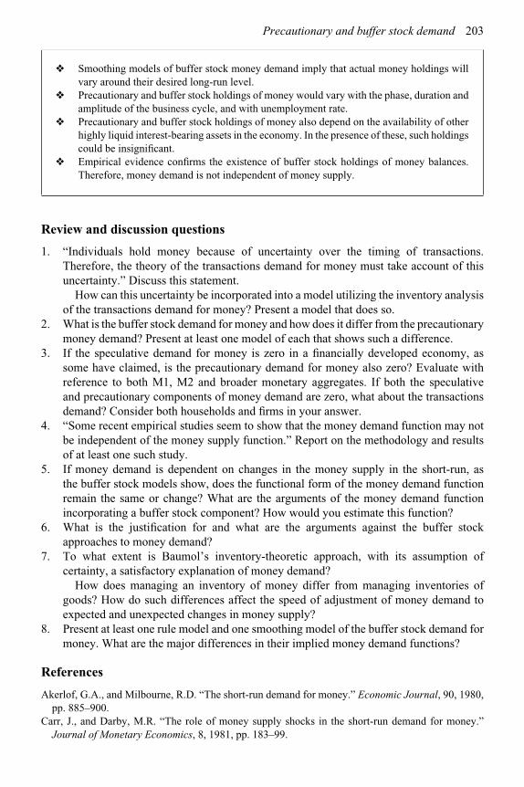
Precautionary and buffer stock demand 203
❖ Smoothing models of buffer stock money demand imply that actual money holdings willvary around their desired long-run level.
❖ Precautionary and buffer stock holdings of money would vary with the phase, duration andamplitude of the business cycle, and with unemployment rate.
❖ Precautionary and buffer stock holdings of money also depend on the availability of otherhighly liquid interest-bearing assets in the economy. In the presence of these, such holdingscould be insignificant.
❖ Empirical evidence confirms the existence of buffer stock holdings of money balances.Therefore, money demand is not independent of money supply.
Review and discussion questions
1. “Individuals hold money because of uncertainty over the timing of transactions.Therefore, the theory of the transactions demand for money must take account of thisuncertainty.” Discuss this statement.
How can this uncertainty be incorporated into a model utilizing the inventory analysisof the transactions demand for money? Present a model that does so.
2. What is the buffer stock demand for money and how does it differ from the precautionarymoney demand? Present at least one model of each that shows such a difference.
3. If the speculative demand for money is zero in a financially developed economy, assome have claimed, is the precautionary demand for money also zero? Evaluate withreference to both M1, M2 and broader monetary aggregates. If both the speculativeand precautionary components of money demand are zero, what about the transactionsdemand? Consider both households and firms in your answer.
4. “Some recent empirical studies seem to show that the money demand function may notbe independent of the money supply function.” Report on the methodology and resultsof at least one such study.
5. If money demand is dependent on changes in the money supply in the short-run, asthe buffer stock models show, does the functional form of the money demand functionremain the same or change? What are the arguments of the money demand functionincorporating a buffer stock component? How would you estimate this function?
6. What is the justification for and what are the arguments against the buffer stockapproaches to money demand?
7. To what extent is Baumol’s inventory-theoretic approach, with its assumption ofcertainty, a satisfactory explanation of money demand?
How does managing an inventory of money differ from managing inventories ofgoods? How do such differences affect the speed of adjustment of money demand toexpected and unexpected changes in money supply?
8. Present at least one rule model and one smoothing model of the buffer stock demand formoney. What are the major differences in their implied money demand functions?
References
Akerlof, G.A., and Milbourne, R.D. “The short-run demand for money.” Economic Journal, 90, 1980,pp. 885–900.
Carr, J., and Darby, M.R. “The role of money supply shocks in the short-run demand for money.”Journal of Monetary Economics, 8, 1981, pp. 183–99.
204 The demand for money
Cuthbertson, K. The Supply and Demand for Money. Oxford: Basil Blackwell, 1985, pp. 30–2,35–9, 130–43.
Cuthbertson, K., and Taylor, M.P. “The demand for money: a dynamic rational expectations model.”Economic Journal, 97, 1987, pp. 65–76.
Darby, M.R. “The allocation of transitory income among consumers’ assets.” American EconomicReview, 62, 1972, pp. 928–41.
Faig, M., and Jerez, B. “Precautionary balances and the velocity of circulation of money.” Journal ofMoney, Credit and Banking, 39, 2007, pp. 843–73.
Kanniainen, V., and Tarkka, J. “On the shock-absorption view of money: international evidence fromthe 1960’s and 1970’s.” Applied Economics, 18, 1986, pp. 1085–101.
Milbourne, R. “Disequilibrium buffer stock models: a survey.” Journal of Economic Surveys, 2, 1988,pp. 187–208.
Miller, M.H., and Orr, D. “A model of the demand for money by firms.” Quarterly Journal of Economics,80, 1966, pp. 413–35.
Mizen, P. Buffer Stock Models and the Demand for Money. London: St Martin’s Press, 1994, Chs. 1–3.Santomero, A.M., and Seater, J.J. “Partial adjustment in the demand for money: theory and empirics.”
American Economic Review, 71, 1981, pp. 566–78.Sprenkle, C.M., and Miller, M.H. “The precautionary demand for narrow and broad money.”
Economica, 47, 1980, pp. 407–21.Whalen, E.L. “A rationalization of the precautionary demand for cash.” Quarterly Journal of
Economics, 80, 1966, pp. 314–24.