arX

iv:1

310.

3740

v1 [

astr

o-ph

.CO

] 1

4 O

ct 2

013

Mon. Not. R. Astron. Soc. 000, 000–000 (0000) Printed 15 October 2013 (MN LATEX style file v2.2)

Halo Abundance Matching: accuracy and conditions for

numerical convergence

AnatolyKlypin1⋆, Francisco Prada2,3,4, GustavoYepes5,

SteffenHeß6, StefanGottlober61, Astronomy Department, New Mexico State University, MSC 4500, P.O.Box 30001, Las Cruces, NM, 880003-8001, USA2 Instituto de Fsica Teorica, (UAM/CSIC), Universidad Autonoma de Madrid, Cantoblanco, E-28049 Madrid, Spain3 Campus of International Excellence UAM+CSIC, Cantoblanco, E-28049 Madrid, Spain4 Instituto de Astrofsica de Andaluca (CSIC), Glorieta de la Astronoma, E-18080 Granada, Spain5 Departamento de Fisica Teorica, Modulo C-15, Facultad de Ciencias, Universidad Autonoma de Madrid, 28049 Cantoblanco, Madrid, Spain6 Leibniz-Institut fur Astrophysik (AIP), An der Sternwarte 16, D-14482 Potsdam, Germany

15 October 2013

ABSTRACT

Accurate predictions of the abundance and clustering of dark matter haloes play akey role in testing the standard cosmological model. Here, we investigate the accuracyof one of the leading methods of connecting the simulated dark matter haloes withobserved galaxies – the Halo Abundance Matching (HAM) technique. We show howto choose the optimal values of the mass and force resolution in large-volume N -bodysimulations so that they provide accurate estimates for correlation functions and circu-lar velocities for haloes and their subhaloes – crucial ingredients of the HAM method.At the 10% accuracy, results converge for ∼50 particles for haloes and ∼150 particlesfor progenitors of subhaloes. In order to achieve this level of accuracy a number of con-ditions should be satisfied. The force resolution for the smallest resolved (sub)haloesshould be in the range (0.1 − 0.3)rs, where rs is the scale radius of (sub)haloes. Thenumber of particles for progenitors of subhaloes should be ∼ 150. We also demonstratethat the two-body scattering plays a minor role for the accuracy of N -body simula-tions thanks to the relatively small number of crossing-times of dark matter in haloes,and the limited force resolution of cosmological simulations.

Key words: cosmology: large-scale structure of the Universe – cosmology: theory –methods: numerical

1 INTRODUCTION

The standard ΛCDM cosmological model phases signifi-cant challenges when it comes to testing its predictions forthe distribution and properties of galaxies. The model isable to make detailed predictions on the distribution ofdark matter, but connecting the luminous galaxies withtheir dark matter haloes is a difficult task. There are dif-ferent possibilities to make this galaxy-halo connection.Halo Abundance Matching (HAM) is a simple and yet re-alistic way to bridge the gap between dark matter haloesand galaxies (Kravtsov et al. 2004a; Tasitsiomi et al. 2004;Vale & Ostriker 2004; Conroy et al. 2006; Guo et al. 2010;Trujillo-Gomez et al. 2011; Reddick et al. 2012; Kravtsov2013). HAM resolves the issue of connecting observed galax-ies to simulated haloes and subhaloes by setting a cor-respondence between the stellar and halo masses: more

⋆ E-mail: aklypin@nmsu.edu

luminous galaxies are assigned to more massive haloes.By construction, the method reproduces the observed stel-lar mass and luminosity functions. It also reproduces thegalaxy clustering over a large range of scales and redshifts(Conroy et al. 2006; Guo et al. 2010; Trujillo-Gomez et al.2011; Reddick et al. 2012; Nuza et al. 2013). When HAM isapplied using, for example, the observed SDSS stellar massfunction (Li & White 2009), it gives also a reasonable fitto lensing results (Mandelbaum et al. 2006), to the galaxyclustering and the relation between stellar and halo virialmasses (Guo et al. 2010). Trujillo-Gomez et al. (2011) showthat accounting for baryons drastically improves the matchof predicted and observed Tully-Fisher and Baryonic Tully-Fisher relations. HAM modeling was also successful in re-producing other properties of galaxies (Behroozi et al. 2010;Leauthaud et al. 2011a; Reddick et al. 2012; Hearin et al.2012; Kravtsov 2013).

Yet, using the HAM technique to connect galaxies to(sub)haloes requires substantially more accurate N-body

c© 0000 RAS

2 Klypin et al.

simulations as compared with those used for the Halo Occu-pation Distribution (HOD) model (Kravtsov et al. 2004a;Tasitsiomi et al. 2004; Vale & Ostriker 2004). Because ofthe demanding numerical requirements, there are relativelyfew studies of abundance and clustering of haloes basedon circular velocities, which are often used in conjunctionwith HAM models (Klypin et al. 2011; Trujillo-Gomez et al.2011; Reddick et al. 2012; Guo & White 2013). Accuracyof these statistics was challenged by Guo & White (2013),who found a very poor numerical convergence of resultsfor subhalo population in the Millennium I (Springel et al.2005) and Millennium II (Boylan-Kolchin et al. 2009) sim-ulations. Though we find much better convergence in ourBolshoi and suite of MultiDark simulations, we agree withGuo & White (2013) that it is important to investigate theaccuracy and limits of HAM technique to connect galaxieswith (sub)haloes using only N-body simulations. In particu-lar, physically robust results demand that statistics such asthe abundance and clustering of subhaloes to be unaffectedby numerical resolution.

Many large volume N-body cosmological simulationsare not suited and should not be used for HAM models. Thenumerical and physical processes which affect the accuracyof results based on cosmological simulations were discussedin many publications (e.g., Knebe et al. 2000; Klypin et al.2001; Power et al. 2003; Hayashi et al. 2003). It is one ofthe goals of this paper to find conditions, that a simulationshould pass in order to be used for HAM models.

The key ingredient of HAM models are subhaloes: satel-lites (subhaloes) of distinct haloes must be part of the abun-dance matching prescription because each lump of dark mat-ter with enough mass and concentration should host a galaxyregardless whether that is the central object or a satellite.We call a halo distinct if its center is not inside the virialsphere of even a larger halo. By definition, a subhalo is al-ways within the virial radius of another halo, which in thiscase is called parent halo. In the sense of dynamical evo-lution subhaloes are different objects because their physicalproperties can be significantly affected (mostly through tidalstripping) by their parent haloes (Tasitsiomi et al. 2004;Kravtsov et al. 2004b). In reality, the boundary separat-ing distinct haloes and subhaloes is blurry. First, there aredifferent definitions of virial radius. As a result, the sameobject can be called distinct or subhalo depending on thevirial ghalo definition. Second, distinct haloes may expe-rience strong interaction with their environment long be-fore they formally cross the virial radius of their parent(Kravtsov et al. 2004b; Behroozi et al. 2013a). In that re-spect some distinct haloes evolve as subhaloes.

There are different flavors of HAMs. Generally, one doesnot expect a pure monotonic relation between stellar andhalo masses. There should be some degree of stochasticityin this relation due to deviations in the halo merger his-tory, angular momentum, and concentration. Even for haloes(or subhaloes) with the same mass, these properties shouldbe different for different systems, which would lead to de-viations in stellar mass. Observational errors are also re-sponsible in part for the non-monotonic relation betweenhalo and stellar masses. Most of modern HAM models al-ready implement prescriptions to account for the stochas-ticity (e.g., Behroozi et al. 2010; Trujillo-Gomez et al. 2011;Leauthaud et al. 2011a). The difference between monotonic

and stochastic models depends on the magnitude of the scat-ter and on the stellar mass. The typical value of the scatterin the r-band is expected to be ∆Mr = 0.3–0.5 mag (e.g.,Trujillo-Gomez et al. 2011). For the Milky Way-size galax-ies the differences are practically negligible (Behroozi et al.2010).

Because haloes may experience tidal stripping, theirdark matter mass may be significantly reduced (e.g.Klypin et al. 1999a; Hayashi et al. 2003; Kravtsov et al.2004b; Arraki et al. 2012). Galaxies hosted by these strippedhaloes are not expected to lose their stellar mass to the samedegree as the dark matter mass because the stellar compo-nent is much more concentrated and thus less susceptibleto tidal forces. This is the reason why the halo dark mat-ter mass is expected to be a poor indicator of the stellarmass of galaxy hosted by the halo. There are quantities thatshould work better for HAM and are often used as prox-ies for stellar mass: dark matter mass before the strippingstarted, maximum circular velocity of the dark matter orthe maximum circular velocity of the dark matter beforethe stripping (e.g., Conroy et al. 2006; Trujillo-Gomez et al.2011; Reddick et al. 2012).

Here we use the maximum circular velocity, not mass.The maximum is reached in the central halo region, whichis expected to correlate better with the stellar or luminouscomponent and it is less sensitive to tidal stripping. This isthe main reason why in this paper we focus our numericalconvergence study on the abundance and clustering statis-tics related with the (sub)halo circular velocities.

While the maximum circular velocity is a betterquantity to characterize (sub)haloes (Conroy et al. 2006;Klypin et al. 2011; Trujillo-Gomez et al. 2011), it is moredifficult to accurately measure it in numerical simulations.For example, for galaxy-size haloes the maximum of the cir-cular velocity happens at ∼ 1/5 of the virial radius. Atthis radius, the resolution should be sufficient to estimatethe maximum circular velocity with better than, say, an ac-curacy better than 10 percent. In addition, subhaloes alsoshould be resolved and their circular velocities are estimated.Thus, the resolution of simulations intended for HAM mod-els should be at least an order of magnitude better thanthose intended, for example, for HOD models.

Our paper is organized as follows. In Section 2 wepresent simulations used for our analysis and discuss haloidentification. Section 3 gives results on the abundance ofhaloes and subhaloes. The numerical convergence study ofthe correlation function for (sub)haloes selected by the max-imum circular velocity is discussed in Section 4. In Section 5we investigate numerical and physical processes, which af-fect accuracy of cosmological N-body simultions. Here wealso provide the conditions for the numerical convergence ofHAM results. Our results are summarized in Section 6

2 SIMULATIONS AND DARK MATTER

HALOES

In order to study the numerical convergence of cosmolog-ical N-body simulations we use three large simulations,which cover a mass range of five orders of magnitude. Thesame cosmological parameters were used for the simula-tions. The simulations were performed using two codes:

c© 0000 RAS, MNRAS 000, 000–000

HAM: conditions for convergence 3

Table 1. Basic parameters of the cosmological simulations. Lbox is the side length of the simulation box, Np is the number of simulationparticles, ǫ is the force resolution in comoving coordinates, Mp refers to the mass of each simulation particle, and the parameters Ωm,ΩΛ , Ωb, ns (the spectral index of the primordial power spectrum), h (the Hubble constant at present in units of 100 km/sMpc−1)and σ8 (the rms amplitude of linear mass fluctuations in spheres of 8 h−1Mpc comoving radius at redshift z = 0) are the ΛCDMcosmological parameters assumed in each simulation.

Name Lbox Np ǫ Mp Ωm ΩΛ ns h σ8 code reference(h−1 Mpc) (h−1 kpc) (h−1M⊙)

Bolshoi 250 20483 1 1.35 108 0.27 0.73 0.95 0.70 0.82 ART Klypin+10MultiDark 1000 20483 7 8.67 109 0.27 0.73 0.95 0.70 0.82 ART Prada+12BigMultiDark 2500 38403 10 2.06 1010 0.27 0.73 0.95 0.70 0.82 LGadget-2 Hess+13

Millennium 500 21603 5 8.61 108 0.25 0.75 1.00 0.73 0.90 Gadget-2 Springel+05Millennium-II 100 21603 1 6.89 106 0.25 0.75 1.00 0.73 0.90 Gadget-3 Boylan-

Kolchin+09

the Adaptive Refinement Tree (ART Kravtsov et al. 1997;Gottlober & Klypin 2008) and Gadget (Springel 2005). De-tails of the ART simulations Bolshoi and MultiDark weregiven in Klypin et al. (2011) and Prada et al. (2012). Thesimulation done with the Gadget is from a large suit ofBigMultiDark simulations(Hess et al. 2013). Main param-eters of our simulations are presented in Table 1, where wealso present parameters of the two Millennium simulations(Springel et al. 2005; Boylan-Kolchin et al. 2009). The tablehighlights one substantial difference between our simulationsand Millennium: our force resolution is substantially betterfor the same mass resolution. Another difference, which isnot shown in the table is that we systematically use signifi-cantly smaller time-steps.

The choice of numerical parameters (combination ofmass, force, and time resolutions) in our simulations is notaccidental. We made many tests (some of them discussedbelow) studying the convergence of results.

We use the Bound Density Maxima (BDM) spheri-cal overdensity code (Klypin & Holtzman 1997; Riebe et al.2011) to identify and find the properties of haloes and sub-haloes in all our simulations. The code was extensively testedand compared with other halofinders (Knebe et al. 2011;Behroozi et al. 2013b; Knebe et al. 2013). Halo tracking wasmade for two simulations (Bolshoi and MultiDark) using theROCKSTAR code (Behroozi et al. 2013b). No halo trackingso far is available for the bigMultiDark simulation.

The BDM halo finder provides many parameters foreach (sub)halo including the virial mass, concentration, andspin parameter. It also includes the maximum circular ve-locity Vmax =

√

GM(r)/r|max. For Bolshoi and MultiDarkwe also find the peak of Vmax over the history of evolutionof each halo and subhalo. This is done using the informationover the history of the major progenitor of each halo. Thepeak velocity Vpeak serves as proxy for the rotation velocityof the galaxy hosted by its halo. This is why Vpeak plays akey role for HAM models. However, from the point of viewof the accuracy of simulations, Vmax is a more importantquantity with Vpeak simply considered to be mapping Vmax.

The virial radius for distinct haloes is defined as radiuswithin which the mean matter density is equal to the virialoverdensity found from the solution of the top-hat model forcosmological model with a cosmological constant. For ourset of cosmological parameters this corresponds to a matter

Figure 1. Cumulative velocity function of dark matter haloesat z = 0 for Bolshoi and Multidark simulations. Here we usethe maximum circular velocity Vpeak over the merging historyof each halo. Bottom panel: Top curves show the total numberof haloes (distinct + subhaloes). Bottom curves show subhaloesonly. Full (dashed) curves are for the Multidark (Bolshoi) simu-lation. Top panel: the ratio of the number of haloes in Bolshoiand Multidark simulations. The full curves show all haloes. Thelong and short dash curves show distinct and subhaloes respec-tively. At the 10% level the total number of haloes converge forVpeak > 140 km s−1. Convergence for subhaloes is reached forlarger velocities Vpeak = 200 km s−1, corresponding to 150 parti-cles in the MultiDark simulation.

overdensity of 360 times the average matter density in theuniverse.

When studying convergence of numerical results, wequote the number of particles within the virial radius. Sub-halos normally do not extend to virial radius because theirradius is truncated by tidal stripping. In order to make thenumber of particles in haloes and subhalos compatible, forsubhalos we quote the number of particles inside the virialradius of a distinct halo with the same maximum circular

c© 0000 RAS, MNRAS 000, 000–000

4 Klypin et al.

Figure 2. Comparison of velocity functions in simulations with vastly different resolutions. Bottom panel: Top curves are total number ofhaloes. Lower curves show only subhaloes. Dashed, full, and dot-dashed curves are for Bolshoi, MultiDark and BigMultiDark respectively.Two top panels show the ratios of all haloes and subhaloes for different pairs of simulations as labeled in the plot.

velocity Vmax as that of the subhalo. The extrapolation tothe virial radius depends on halo concentration. We use theaverage virial mass - Vmax relation for distinct halos to makethe extrapolation to the virial radius. The actual number ofparticles in a subhalo can only be smaller than the extrap-olated value. We find that the extrapolated virial masses ofsubhalos are within 10–20% of virial masses of 90% of pro-genitors of the subhalos defined at the moment of the peakof Vmax. This is why we call these estimates of the subhalomasses and number of particles the masses and particlesnumbers of subhalo progenitors.

3 HALO VELOCITY FUNCTION

We start with the analysis of the velocity functions usingthe peak values of Vmax in Bolshoi and MultiDark. Fig-ure 1 shows the velocity functions separately for subhaloesand the total populations of haloes. Overall there is anexcellent agreement between both simulations for a widerange of circular velocities Vpeak = 200−1000 km s−1, where(sub)haloes are resolved with enough particles and the cos-mic variance does not effect the results. At large velocities(Vpeak > 1000 km s−1 there are clearly some effects due tothe lack of long waves and cosmic variance in the Bolshoisimulation due to its smaller box size. Deviations of thenumber of haloes at small velocities Vpeak < 200 km s−1

are indication of numerical resolution effects in the Multi-Dark simulation. The smaller number of haloes in Multidark

c© 0000 RAS, MNRAS 000, 000–000

HAM: conditions for convergence 5

at smaller velocities are due to the lack of force and massresolution as compared to Bolshoi (see Table 1).

At the 10% level of accuracy the number-density ofhaloes converge for peak velocities Vpeak > 140 km s−1,which corresponds to the average number of 52 particlesinside the virial radius in the Multidark simulation. As ex-pected, convergence is worse for subhaloes. However, it isstill very good: at 10% it is Vpeak = 200 km s−1. For iso-lated haloes this corresponds to an average of 150 particles.This is a remarkably small number of particles. For com-parison, convergence of the velocity function of subhaloesin the Millennium simulations, at the same accuracy level,was achieved only with ∼ 3000 particles (see Guo & White2013)

Accuracy of HAM results depends on a number of nu-merical effects. Each of them should produce small enougherrors so that the final result can be trustful. The effects in-clude the tracking of subhaloes as they fall into larger haloesand become subhaloes (Behroozi et al. 2010). Other effectsinclude mass and force resolution, time-integration of equa-tions of motion, and two-body scattering. Accuracy of halotracking was discussed in Behroozi et al. (2010). Here wefocus on the other effects. In order to study those, we inves-tigate the statistics based on the instantaneous maximum ofthe circular velocity Vmax.

Figure 2 presents the results of three simulations: Bol-shoi, MultiDark, and BigMultiDark. To large degree theresults are very similar to those based on Vpeak. Again,the comparison between Bolshoi and MultiDark shows con-vergence at 10% level for distinct haloes with Vmax >140 km s−1 and for subhaloes with Vmax > 200 km s−1. Thisimplies that subhaloes need about 150 particles to have thisaccuracy. The comparison between BigMultiDark and Mul-tiDark shows the same, i.e. in order to reach the 10% accu-racy, one needs ∼ 150 particles for subhaloes.

4 CONVERGENCE OF THE CORRELATION

FUNCTION

Convergence of the two-point correlation function for haloesand subhaloes, selected by either Vpeak or Vmax, is demon-strated in Figures 3 and 4, where we compare results forBolshoi and MultiDark. Just as for the circular velocityfunctions, the agreement of the results on small scales (.2h−1 Mpc) indicates convergence of the results regaring thenumerical parameters such as mass and force resolution. Thedifferences in correlation functions on larger scales are dueto finite box size and cosmic variance.

On scales 0.2h−1 Mpc < R < 1h−1 Mpc the agreementbetween Bolshoi and MultiDark is about 5%, with Bolshoiexhibiting slightly larger clustering signal as expected dueto it better force and mass resolution (see Table 1). Thesituation is unclear on even smaller scales mostly becauseof very small number of pairs within these separations (andthus large noise) in Bolshoi.

Because of much larger statistics of halos in MultiDarkand BigMultiDark simulations, the level of shot noise on∼ 100 h−1 kpc scales is smaller, which allows us to test thosesimulations on these scales. Indeed, in this case the convergeof results is substantially better as illustrated by Figure 5. Itis also much better on large scales due to sugnificantly larger

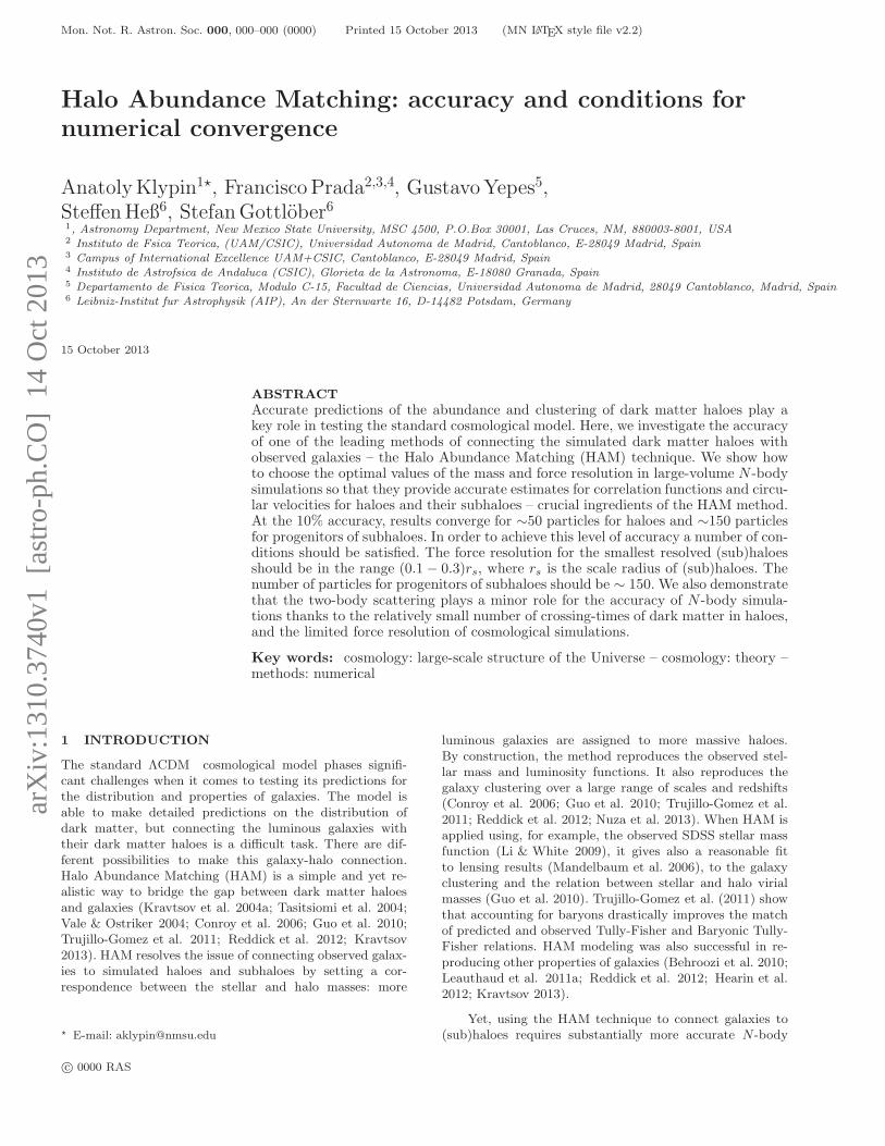
Figure 3. Comparison of the correlation functions for haloes inthe MultiDark (full) and Bolshoi (dashed) simulations. Haloeswere selected to have their peak circular velocities (maximumcircular velocity over the accretion history of each halo) to belarger than Vpeak > 200 km s−1 for the bottom panel and Vpeak >220 km s−1 for the top panel. Because of the lack of long waves inthe Bolshoi, the correlation function in the MultiDark is larger forscales above 2h−1 Mpc. Clustering at smaller scales is not affectedby long waves and it is a test of numerical effects and convergenceof simulations. At the 5% level the correlation functions agree forboth simulations. For the MultiDark simulation, velocity limitVpeak > 200 km s−1 corresponds on average of 160 particles.

Figure 4. The same as in Figure 3, but for haloes selected bythe maximum circular velocity Vmax. Clustering at scales below2h−1 Mpc indicate convergence of results at ∼ 5% level for haloeswith more than ∼ 150 particles.

c© 0000 RAS, MNRAS 000, 000–000

6 Klypin et al.

Figure 5. Correlation functions of haloes in the MultiDark (full)and BigMultiDark (dashed) simulations. Haloes were selected tohave the maximum circular velocity Vmax > 240 km s−1, whichon average corresponds to 120 particles. Both simulations havenearly the same (within few percent) correlation functions from100 h−1 kpc to 40h−1 Mpc. At larger distances the correlationfunction in the MultiDark is below that of BigMultiDark becauseof the cosmic variance. The dot-dashed curve represents the linearcorrelation function scaled up with bias factor 1.3. It shows thaton scales larger than ∼ 30h−1 Mpc clustering of haloes has anearly scale-independent bias. The correlation function aroundthe BAO peak is slightly damped and broadened by non-lineareffects.

box sizes. Both simulations have nearly the same (withinfew percent) correlation functions from ∼ 100 h−1 kpc to40 h−1 Mpc. One starts to run on substantially larger dif-ferences on scales below ∼ 100 h−1 kpc. This is due to acombination of force resolution and real-space halofinder,which misses subhalos, when their centers are too close tothe center of parent halo.

Another interesting statistics, which can be used toprobe the numerical convergence, is the halo-dark mattercross correlation function ξhdm. It is an important quantityon its own because it is required for theoretical predictionsof the weak galaxy lensing signal (e.g., Leauthaud et al.2011b). Figure 6 shows ξhdm for MultiDark and BigMul-tiDark with halos selected at the low limit of resolution:Vmax = (250 − 270)km s−1. The difference between thesimulations is less than ∼ 2% for scales larger than ∼150 h−1 kpc. There is a 5–10% error on scales . 100 h−1 kpcwith the lower-resolution BigMultiDark simulation predict-ing stronger clustering signal. By using simple N-body toymodels we find that the reason for this extra clustering isdue to a side-effect of force resolution. Because of lack of res-olution, the dark matter, which should have been at smalldistances, ends up at larger distances, where it slightly in-creases the local density and, thus, increases the cross cor-relation signal.

On scales above 2h−1 Mpc the correlation function in

Figure 6. Bottom panel: Cross correlation function of halos anddark matter in MultiDark (full) and BigMultiDark (dash) simula-tions. Top panel: Ratio of the cross correlation functions. Distincthalos with Vmax = (250 − 270)km s−1 were used.

Bolshoi is systematically lower than in MultiDark. Thelarge-scale differences between Bolshoi and Multidark sim-ulations are likely due to both the cosmic variance and thefinite box size. It is easy to test the effect of box size. Forthat, we estimate the correlation function using linear the-ory and truncate the power spectrum at the lower wavenum-ber limit given by the fundamental mode of the simulationbox: kBox = 2π/L, where L is the length of computationalbox. Figure 7 shows correlation functions of the dark matter,which are obtained for different box sizes.

As expected, the finite size of the simulation box af-fects the large scales in a profound way. For example, forthe L = 100 h−1 Mpc box used in the Millinium-II simu-lation (Boylan-Kolchin et al. 2009), the correlation functionbecomes negative for R > 25h−1 Mpc while it should be pos-itive. Even smaller scales are affected: at R = 10h−1 Mpcthe correlation function is 30% below the true one (solidcirve in Figure 7. Note that often used a rule of thumb thatscales smaller than 1/10 of the box length are not affectedby the box size, does not really hold. Indeed, the deviationsof the linear correlation function at R = L/10 strongly de-pend on the box length L. One may expect that nonlineareffects exacerbate the differences.

Because of the box size effects, the comparison betweensimulations on large scales should be done using a large boxsize. Indeed, the converge of results is substantially betterfor large-box simultions. Figure 5 illustrates this point bycomparing MultiDark and BigMultiDark simulations withL = 1 h−1Gpc and L = 2.5 h−1Gpc. Both simulations havenearly the same (within few percent) correlation functionsfrom 100 h−1 kpc to 40h−1 Mpc for haloes and progenitorsof subhaloes with ∼ 150 particles.

Convergence and accuracy of halo clustering and abun-dances in our set of simulations are significantly better –

c© 0000 RAS, MNRAS 000, 000–000

HAM: conditions for convergence 7

Figure 7. Effects of the finite simulation box size on the corre-lation function. We use the linear power spectrum scaled up bythe bias factor b = 1.7 to calculate the correlation functions. Inorder to mimic the lack of long waves in simulations of differentbox sizes, the integral over the power spectrum is truncated atkBox = 2π/L, where L is the size of the computational box. Thelack of long waves in small boxes results in significant suppressionof clustering at scales even as small as 1/10 of the computationalbox.

by a factor of 20 in mass – than for the Millennium simula-tions (Guo & White 2013). As a way to compensate the lackof resolution in the Millennium simulations, a trick is used:if a subhalo is lost, it is assigned to the most bound darkmatter particle of this subhalo, and called an “orphan”. Asimplified dynamical friction estimate is then used to set aclock when the subhalo is assumed to merge with its par-ent (Guo et al. 2011). It is not clear to us what causes sucha poor performance of the Millennium simulations. This isnot related with the N-body code: we achieve satisfactoryresults aslo with the Gadget code. There are some concernsregarding the Millennium simulations, but none of them se-pearately seems to be enough to explain the poor conver-gence in the Millennium simulations. For example, the num-ber of time-steps is low. For the Millennium-I run the param-eter ErrTolIntAccuracy= 0.01, which defines the number ofsteps, is twice larger than what we use in our Gadget simu-lation bigMultidark. The force resolution is also low in theMillennium simulations. In addition, the small size of thecomputational box of the Millennium-II run raises doubtsthat it was large enough to provide the true solution whencompared with the Millennium-I. It is possible that a com-bination of all these small defects resulted in much worseresults for subhaloes. We highlight that the better accuracyof our simulations eliminates the need for “orphans” in oursimulations.

5 CONDITIONS FOR CONVERGENCE

Usually, numerical convergence of cosmological simulationsis discussed in the context of simulations of individual darkmatter haloes with large number of particles. For exam-ple, convergence of dark matter density profiles is studiedby running simulations with increasing very large numberof particles (e.g. Klypin et al. 2001; Springel et al. 2008;Stadel et al. 2009). Here, we are interested in convergenceon the opposite side of the spectrum: how reliable are re-sults with very small number of particles? The small haloesare very important. After all, most of haloes in each simu-lation are tiny, and numerous statistics (e.g. the halo massfunctions) use those small halos. Results presented in Sec-tion 3 indicate convergence of the velocity function of dis-tinct haloes with ∼ 50 particles. How can we understandthis?

The accuracy and convergence of results used for haloabundance matching depend on a number of physical andnumerical processes. We split those into two categories: (a)accuracy of the maximum circular velocity Vmax for isolatedhaloes and (b) physics and numerics of subhaloes. We focuson some rather specific problems, which to large degree de-fine convergence of numerical results. The goal is to studythese processes separately by isolating each one and inves-tigating it by using a simple realistic model. In reality, allprocesses are interconnected and only a full-scale cosmo-logical simulation have all all of them included. However,understanding the conditions for convergence of large cos-mological simulations is difficult because it is not clear whatare the processes and how they potentially affect the results.We get much better insights by studying separate processes.

5.1 Accuracy of circular velocities of isolated

haloes

Here we consider three effects: (a) force resolution, (b) massresolution (number of particles) and (c) two-body scattering.We investigate a series of simulations of isolated NFW halos.In all cases we start with a NFW halo, which is set in equi-librium. The equilibrium initial conditions are constructedassuming an ideal phase-space distribution function for aNFW halo with isotropic velocities and with no correctionfor force softening or discreteness. Because of different nu-merical effects – the force softening, discreteness effects, andtime-stepping – the system of N particles does not stay inthe equilibruim. It evolves. In most of the cases, the systemreaches another equilibrium after few dynamical times. Bycomparing this new state with the initial one, we estimatethe magnitude of the numerical effect responsible for theevolution.

When dealing with the NFW halo, it is convenient toexpress all physical quantities using the scale radius rs andthe maximum circular velocity Vmax. Those quantities arerelated to the virial mass Mvir and concentration c through

c© 0000 RAS, MNRAS 000, 000–000

8 Klypin et al.

the following relations:

V 2max =

GMvir

Rvir

f(xmax)

f(c)

c

xmax

, (1)

c =Rvir

rs, x ≡ r

rs, xmax = 2.163 (2)

M(x) = Mvirf(x)

f(c), f(x) = ln(1 + x)− x

1 + x, (3)

V 2(x) = V 2max

xmax

x

f(x)

f(xmax)(4)

ρ(x) =V 2max

4πGr2s

xmax

f(xmax)

1

x(1 + x)2. (5)

Written in this way, the halo structure does not depend onc and Mvir. This allows us to simulate just one system andthen to rescale it to any particular values of Mvir and c.

It is convenient to use some fiducial virial radius andvirial mass. For this, we use concentration c = 8 and fiducialvirial radius 8 rs which are typical parameters for galaxy-sizehaloes with mass Mvir = 1012h−1M⊙ (Prada et al. 2012).A useful scale for time is the crossing-time at the radiusrmax = 2.163 rs, at which the circular velocity reaches themaximum Vmax:

tcross ≡rmax

σv(rmax)≈ xmax

rsVmax

, (6)

where σv(rmax) is the 3D r.m.s. velocity at rmax. Thecrossing-time in physical units depends on halo concentra-tion. For virial mass defined at overdensity 200 ρcr, where ρcrbeing the critical density of the Universe, the crossing-timeis:

tcross = 9.8 h−1 f(c)

c3/2Gyrs. (7)

He have tcross = 0.3 Gyr for a Milky Way-type galaxy withc = 8. The crossing-time depends only very weakly on halomass: it is twice smaller for haloes of dwarf galaxies withMvir = 109h−1M⊙ and twice larger for clusters of galax-ies with Mvir = 1015h−1M⊙. Note that haloes do not livelong: during 10 Gyrs of evolution they have only ∼ 20 − 60crossing-times.

Initial density profiles extend to ∼ 50 rs, which is signif-icantly larger than any realistic halo in cosmological simu-lations. All simulations use a simple direct summation codewith a leap-frog integration scheme. The code adopts thePlummer softening (force resolution) ǫ. All simulations weredone with time-steps small enough to have energy conserva-tion |∆E/E| < 10−6.

As a test, we run a simulation with large number ofparticles N = 10, 000 and small force softening ǫ = 0.005 rs.With the exception of very small non-equilibrium effects atthe center, the halo did not change for many dynamical time-scales. However, when simulations are run with either smallN or large ǫ, the haloes do get modified. The comparisonof the evolved halo with its initial equilibrium distributiongives as a way to measure effects of mass and force reso-lution separately. In cosmological simulations haloes growin a complex fashion through merging and accretion. How-ever, at late stages of evolution the accretion slows downand haloes spend most of their time in the regime of slowlygrowing quasi equilibrium NFW distribution. Ability of codeto maintain this equilibrium distribution is an important in-dication of its accuracy.

Figure 8. Effects of the force resolution on the structure of darkmatter haloes. Bottom panel: Circular velocity profiles of haloeswith different force resolutions ǫ. The top dashed curve shows theinitial NFW profile. Each profile is displayed starting with radius2ǫ. Profiles converge to the NFW profile as ǫ decreases. For eachǫ the profile is similar to NFW with larger effective scale radiusand smaller maximum circular velocity. Top panel: dependence ofthe maximum circular velocity on the force resolution. The fullcurve shows approximation equation (9).

5.1.1 Force resolution

We first study the effects of force resolution by studyingrelatively large numerical experiments with 50,000 particleswithin a radius of 10 rs and 100,000 particles in total. Withinthe radius xmax = 2.16 rs the halo has about 15,000 parti-cles. This configuration was simulated with different forceresolutions ranging from ǫ = 0.005 rs to ǫ = 2 rs. Each sim-ulation started with exactly the same initial conditions ofequilibrium NFW halo without any consideration for theforce resolution. For simulations with small ǫ there was verylittle evolution in the distribution of particles. However, inthe cases of large ǫ the force was too weak in the centralregion to keep particles in equilibrium. As the result, eachsimulation with large ǫ evolved starting with the center. Allsimulations with ǫ < rs settled into new equilibrium afterfew crossing-times. The simulation with ǫ = 2 rs was chang-ing even after 5 crossing-times. At this moment the simu-lation was stopped because its very peripheral regions withr > 10 rs were affected.

Figure 8 shows circular velocity profiles for runs withdifferent force resolutions ǫ. Qualitatively the results aresimilar to those found in convergence studies of individ-ual haloes in cosmological simulations: as the resolution in-creases, halo circular velocity profiles converge.

We can use these results to estimate errors in Vmax. Thetop panel in Figure 8 shows the dependance of Vmax on ǫ.At small ǫ the error in Vmax is relatively small. For exam-ple, we have Vmax = 0.98 Vmax,true for ǫ = rs/4. However,the error of Vmax significantly increases with increasing ǫ:

c© 0000 RAS, MNRAS 000, 000–000

HAM: conditions for convergence 9

∆Vmax/Vmax = 0.17 for ǫ = rs. One must keep in mind thatVmax should be quite accurate because the relevant statis-tics, which use Vmax, are very sensitive to it. For example,the abundance of haloes and subhaloes scales with the max-imum circular velocity as n(> Vmax) ∝ Vmax

−3.It is interesting to compare the convergence results in

these experiments with those in our cosmological simula-tions. Our results indicated the convergence of the halo ve-locity function at the 5% accuracy for haloes with Vmax =240 km s−1 in the BigMultiDark simulation. This corre-sponds to haloes with 120 particles and typical scale radiusrs = 30 h−1 kpc. The force resolution is ǫ = 7h−1 kpc for theBigMultiDark. This gives ǫ = 0.23 rs. According to Figure 8the error in Vmax is less than 2%. In turn, the error in thevelocity function n(> Vmax) should be less than 5%, whichis close to what we find in our cosmological simulations.

The following model can be used to make an approxima-tion for the errors in Vmax. We note that profiles of Vmax(r; ǫ)shown in the bottom panel of Figure 8 look similar to theNFW profile, which scale radius is larger and Vmax is smallerthan in the initial NFW halo. At large radii all the velocitycurves converge to the same values because the mass distri-bution at large distances is not affected by the resolution.The increase in the scale radius due to the force resolutioncan be approximated as

rs,ǫ = β(ǫ)rs, β(ǫ) ≈√

1 + (1.7ǫ/rs)2. (8)

Using this expression and normalizing the modified NFWprofile so that at large radii it has the same mass as theinitial NFW, one obtains an approximation for the declineof Vmax due to the force resolution:

(

Vmax,ǫ

Vmax

)

≈ β(ǫ)−1/4 =(

1 + (1.7ǫ/rs)2)−1/4

. (9)

This approximation is shown in the top panel of Figure 8.The increase in the scale radius due to poor force resolu-

tion leads to a decrease in halo concentration. Equation (8)implies that concentration cǫ measured for a halo, which wassimulated with the force resolution ǫ, declines as cǫ = c/β(ǫ).For ǫ/rs = 0.25 this gives 8% error in concentration. If equa-tion (1) is used to find halo concentration from measuredVmax and virial velocity V 2

vir = GMvir/Rvir (e.g. Prada et al.2012), then reqirements to the force resolution are even morestringent. Error analysis shows that in order to have an er-ror in concentration less than 5%, the force softening mustbe smaller than ǫ/rs = 0.1, which in turn implies not morethan 1% error in Vmax.

Equation (8) can be used to recover the true concen-tration c = Rvir/rs. We assume that a simulation, whichis performed with the force resolution ǫ, provides the virialradius Rvir and the concentration cǫ for a halo. The trueconcentration for the halo can be estimaed as:

c =cǫ

√

1− (1.7ǫcǫ/Rvir)2. (10)

These approximations can be used to set the upper limiton the force resolution needed to achieve a given accuracyof the maximum of the circular velocity Vmax. For example,in order to have no more than 2(5)% error in Vmax, the forceresolution should be smaller than ǫ/rs < 0.25(0.40).

5.1.2 Mass resolution

Here we address two issues: (a) are there any systematiceffects that force the value of Vmax, measured in simulationswith small number of particles, to deviate from its true valueand (b) what is the level of statistical fluctuations of Vmax.

In order to address these issues, we made three simula-tions of NFW halos, which were initially in equilibrium, eachwith 300 particles inside radius of 52 rs. These simulationsinitially had only 150 particles within the fiducial virial ra-dius and 25 particles inside rs. This is the smallest number ofparticles, for which our cosmological simulations show con-vergence. Results presented below are averages of the threerealizations. The force resolution is ǫ = 0.2 rs, which is typi-cal for our cosmological simulations for the smallest resolvedhaloes. Results presented in Sec. 5.1.1 indicate that this forceresolution is sufficient for accurate estimates of Vmax.

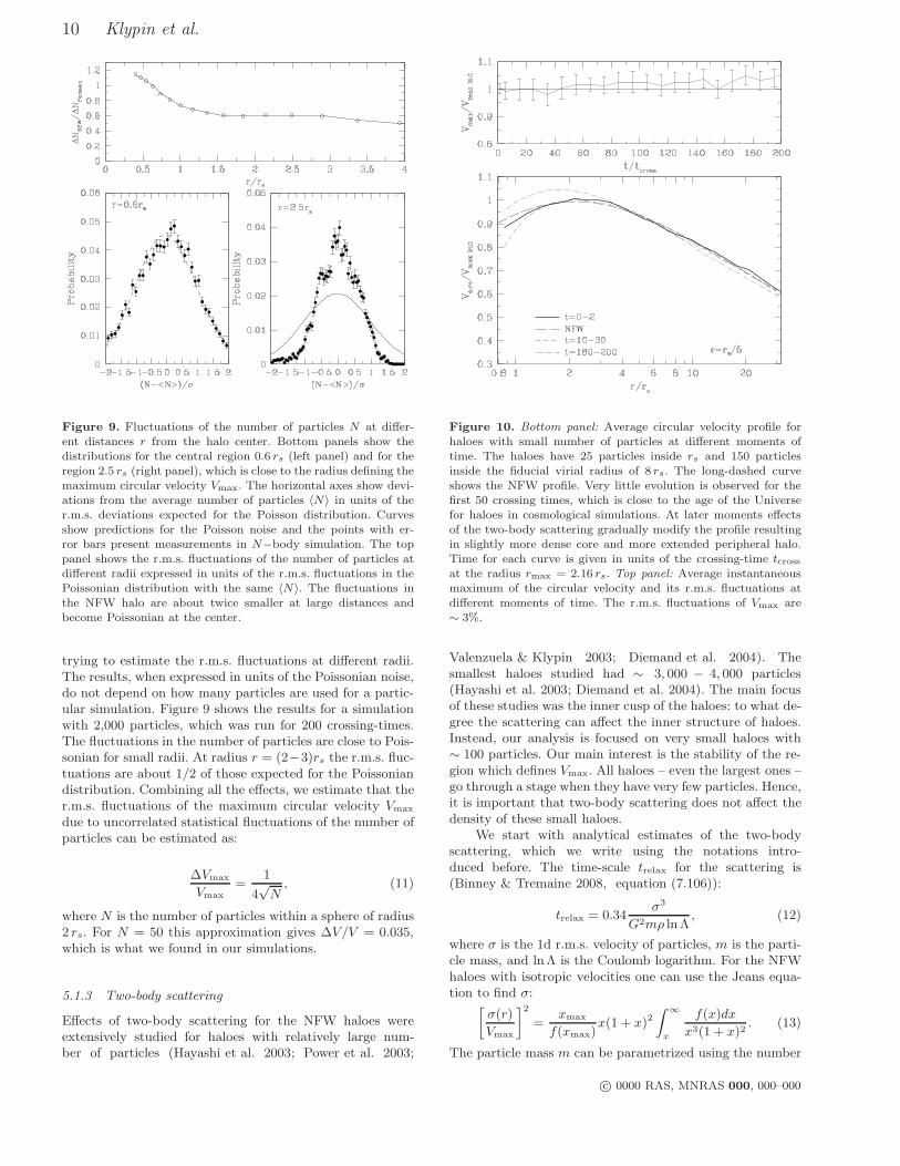
Figure 10 shows the circular velocity profiles in thesesimulations with very small number of particles. We can onlyestimate the velocity profile for distances larger than ∼ rs:there is not enough particles to probe smaller radii. However,on average the models stay close to the initial NFW profile:deviations are less than 5% for radii r = (1− 10)rs and fortime t < 50 tcross.

The simulations indicate that the value of Vmax doesnot show any systematic changes over the same period oftime and that even with 150 particles one can accuratelyestimate Vmax. At later moments Vmax gradually increasespresumably due to accumulation of the two-body scatteringeffects. However, the change is small: 5% after 200 crossingtimes.

In order to measure the level of statistical fluctuationsof Vmax, the value of Vmax is estimated for each snapshotand the statistics is accumulated for many snapshots. Re-sults are presented in the top panel of Figure 10. The level offluctuations of Vmax is just ∼3%, which is remarkably smallconsidering that there are only N ∼50 particles inside theradius rmax = 2.16 rs, which typically defines the maximumof the circular velocity. One would naively expect larger fluc-tuations of ∼ 1/

√N ≈ 15%. The real fluctuations are about

five times smaller.

Assuming that the number of particles N inside a givenradius r is distributed according to the Poissonian statis-tics, we expect that the r.m.s. fluctuations of circular ve-locity are ∆V/V =

√

∆M/M =√

∆N/N , which gives

∆V/V = 1/2√N . Additional reduction in the fluctuations

is related with deviations from the Poissonian noise. Fluctu-ations of the number of particles are actually not expectedto be Poissonian. One can design few examples to illustratethis. Orbital eccentricity should be a factor: there are nofluctuations, if the orbits are circular. For a given radiusthere are always some number of particles, which do nothave energy to leave the radius. These particles always stayinside the radius and, thus, their number does not fluctu-ate. The fraction of these particles depends on the radius.In the central region, r < rs, a large fraction of particles isnot bound to the center. They travel to large distances andonly occasionally are found within the radius r. At large dis-tances the fraction of bound particles increases resulting insmaller fluctuations.

To measure the deviations from the Poissonian statis-tics, we run a number of different numerical experiments

c© 0000 RAS, MNRAS 000, 000–000

10 Klypin et al.

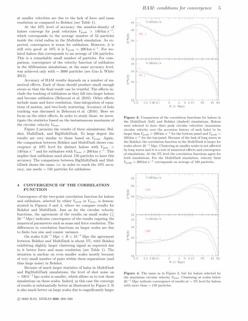
Figure 9. Fluctuations of the number of particles N at differ-ent distances r from the halo center. Bottom panels show thedistributions for the central region 0.6 rs (left panel) and for theregion 2.5 rs (right panel), which is close to the radius defining themaximum circular velocity Vmax. The horizontal axes show devi-ations from the average number of particles 〈N〉 in units of ther.m.s. deviations expected for the Poisson distribution. Curvesshow predictions for the Poisson noise and the points with er-ror bars present measurements in N−body simulation. The toppanel shows the r.m.s. fluctuations of the number of particles atdifferent radii expressed in units of the r.m.s. fluctuations in thePoissonian distribution with the same 〈N〉. The fluctuations inthe NFW halo are about twice smaller at large distances andbecome Poissonian at the center.

trying to estimate the r.m.s. fluctuations at different radii.The results, when expressed in units of the Poissonian noise,do not depend on how many particles are used for a partic-ular simulation. Figure 9 shows the results for a simulationwith 2,000 particles, which was run for 200 crossing-times.The fluctuations in the number of particles are close to Pois-sonian for small radii. At radius r = (2−3)rs the r.m.s. fluc-tuations are about 1/2 of those expected for the Poissoniandistribution. Combining all the effects, we estimate that ther.m.s. fluctuations of the maximum circular velocity Vmax

due to uncorrelated statistical fluctuations of the number ofparticles can be estimated as:

∆Vmax

Vmax

=1

4√N

, (11)

where N is the number of particles within a sphere of radius2 rs. For N = 50 this approximation gives ∆V/V = 0.035,which is what we found in our simulations.

5.1.3 Two-body scattering

Effects of two-body scattering for the NFW haloes wereextensively studied for haloes with relatively large num-ber of particles (Hayashi et al. 2003; Power et al. 2003;

Figure 10. Bottom panel: Average circular velocity profile forhaloes with small number of particles at different moments oftime. The haloes have 25 particles inside rs and 150 particlesinside the fiducial virial radius of 8 rs. The long-dashed curveshows the NFW profile. Very little evolution is observed for thefirst 50 crossing times, which is close to the age of the Universefor haloes in cosmological simulations. At later moments effectsof the two-body scattering gradually modify the profile resultingin slightly more dense core and more extended peripheral halo.Time for each curve is given in units of the crossing-time tcrossat the radius rmax = 2.16 rs. Top panel: Average instantaneousmaximum of the circular velocity and its r.m.s. fluctuations atdifferent moments of time. The r.m.s. fluctuations of Vmax are∼ 3%.

Valenzuela & Klypin 2003; Diemand et al. 2004). Thesmallest haloes studied had ∼ 3, 000 − 4, 000 particles(Hayashi et al. 2003; Diemand et al. 2004). The main focusof these studies was the inner cusp of the haloes: to what de-gree the scattering can affect the inner structure of haloes.Instead, our analysis is focused on very small haloes with∼ 100 particles. Our main interest is the stability of the re-gion which defines Vmax. All haloes – even the largest ones –go through a stage when they have very few particles. Hence,it is important that two-body scattering does not affect thedensity of these small haloes.

We start with analytical estimates of the two-bodyscattering, which we write using the notations intro-duced before. The time-scale trelax for the scattering is(Binney & Tremaine 2008, equation (7.106)):

trelax = 0.34σ3

G2mρ lnΛ, (12)

where σ is the 1d r.m.s. velocity of particles, m is the parti-cle mass, and lnΛ is the Coulomb logarithm. For the NFWhaloes with isotropic velocities one can use the Jeans equa-tion to find σ:

[

σ(r)

Vmax

]2

=xmax

f(xmax)x(1 + x)2

∫

∞

x

f(x)dx

x3(1 + x)2. (13)

The particle mass m can be parametrized using the number

c© 0000 RAS, MNRAS 000, 000–000

HAM: conditions for convergence 11

Figure 11. The same as in Figure 10, but for much finer forceresolution of ǫ = 0.005 rs. Two-body scattering is much morepronounced as compared with large ǫ simulations typically usedin cosmological simulations. Even for unrealistically small ǫ =0.005 rs, the scattering changes Vmax only by 5% for the life-spanof 30–50 tcross of these haloes in cosmological runs.

of particles Nmax inside the radius rmax = 2.16 rs. Combin-ing these expressions and writing the two-body scatteringtime in units of the crossing time (eqs.6 and 7), we get:

trelaxtcross

= 0.344πNmax

ln Λ

[

x(1 + x)2]5/2

x3/2maxf1/2(xmax)

[∫

∞

x

f(x)dx

x3(1 + x)2

]3/2

.

(14)The integral in equation (14) may be taken numerically.However, it can be approximated in a simple way. We notethat the relaxation time depends on the course-grainedphase-space density ρ/σ3, which is know to be nearly apower law. Indeed, the following approximation is accuratewithin 15% for a wide range of radii x = 0.003 − 100:

[

x(1 + x)2]5/2

[∫

∞

x

f(x)dx

x3(1 + x)2

]3/2

≈ x1.92

7.5. (15)

Substituting this into equation (14) and estimating numer-ical factors, we get:

trelaxtcross

= 0.262Nmax

ln Λ

(

r

rs

)1.92

. (16)

The term Λ is the ratio of the maximum bmax to the mini-mum bmin impact parameters for the two-body scatteringproblem. In realistic cosmological simulations and in oursimple numerical models the minimum impact parameter isdefined by the force resolution. For bmin we use the distanceat which the force becomes Newtonian: bmin = 2.8 ǫ. Forbmax one may use the whole region, which is relevant for theinner structure of the NFW distribution bmax ≈ (3− 10)rs.This leads to lnΛ ≈ ln(3rs/ǫ).

We can get another useful approximation for the re-laxation time, if in equation 16 we replace tcross with its

Figure 12. The same as botom panel in Figure 10, but for simu-lations with 50,000 particles inside the fidutial virial radius. Ver-tical lines show radii with 50, 200 and 1,000 particles. Two-bodyscattering is clearly seen at small distances.

value given by equation (7) and also use the number of par-ticles inside a given radius: N(x) = Nmaxf(x)/f(xmax). Thefollowing aprroximation gives tcross for a given halo concen-tration c and a number of particles N(r):

trelax ≈ 1.4h−1GyrsN(r)

c ln(3rs/ǫ)

[

1 +

(

r

rs

)5/4]

. (17)

We can use equations (16) or (17) to estimate trelaxfor our simulations. For simulations presented in Figure 10,Nmax = 45 and one finds trelax = 26 tcross, which is10h−1 Gyrs when scaled to Milky Way-size haloes (c = 10).

Note that during t ≈ trelax the halo density profile doesnot change much: within ∼ 5% the circular velocity profile isthe same as the initial NFW (see Figure (reffig:TwoBody2)).The halo does suffer from the scattering, but on much longertime-scale of t ≈ (5−6) trelax. To some degree, the scatteringin these simulations was suppressed by choosing a reasonableforce resolution, i.e. small enough to resolve well the haloand not too small to avoid excessive scattering. Indeed, werun the same simulations with much smaller force softeningand find that scattering significantly increases. Figure 11shows the results for ǫ = 0.005 rs. It is clear that in this casethe two-body scattering affects the whole halo. However,even for this unrealistic case the scattering changes Vmax

by 5% for the life-span of (30 − 50) tcross of these haloes incosmological runs.

As equation (16) shows, the relaxation time-scale verystrongly depends on radius trelax(r) ∝ r−α, α ≈ −2.This makes the averaging of trelax over the whole halonot very useful for haloes with steep cusps (Quinlan 1996;Hayashi et al. 2003). E.g., a long time-scale of scatteringestimated at half-mass radius does not imply that the scat-tering is negligable because it still may be important close

c© 0000 RAS, MNRAS 000, 000–000

12 Klypin et al.

Figure 13. The density profile in the inner region of the NFWhalo. The full curve shows the density profile after 40 tcross. Theother curves show the initial profile averaged for t = 0 − 2tcross(long-dashed cirve) and the NFW profile (dotted curve). Verticallines show the radii encompassing 50, 200, and 1,000 particles atthe final stage of evolution. The two-body scattering results in thedecline of density in the very center. At the radius encompasing200 particles the decline is less than 3%.

to the halo center. The opposite is also not true: the factthat the scattering time is short at some distance does notmean that the other parts of the halo are affected.

All the results present above indicate that the effectsof two-body scattering are localized, with the outer halo re-gions being basically collisionless. This distance, at whichthe scattering starts to make an effect may or may not beimportant for a particular situation. To illustrate the pointwe made numerical experiments with larger number of par-ticles, which allow us to probe small radii. We simulatedthree realizations of haloes with 50,000 particles inside thefiducial virial radius of 8rs and 105 particles in total. Theforce resolution was ǫ = 0.01 rs. Figure 12 shows that inthese haloes the central region r < 0.2rs is affected by thetwo-body scattering while the outer regions are not. As timegoes on, the radius separating the inner affected region fromour collisionless halo gradually increases.

Note that at the radius containing the first 50 parti-cles the decline in circular velocity is worse for these haloeswith larger number of particles as compared with the previ-ously studied haloes with only 150 particles inside the fidu-cial virial radius. This increase in the scattering at smallradii can be shown analytically using equation (17). Indeed,the number of particles inside radius x with a given valueof trelax must be ∼ 4 times larger for r ≪ rs than forr ≈ rmax = 2.16 rs. In that sense, the two-body scatter-ing has the smallest impact for small haloes. For example,to have trelax = 30 tcross a halo should have ∼ 50 particlesinside x = xmax and ∼ 200 particles inside x = 0.01.

Our results are in overall agreement with those of

Hayashi et al. (2003) when we compare their simulation ofa NFW halo with 3,000 particles and take into accountdifferences in the definitions of the crossing-time and theCoulomb logarithm. Just as Hayashi et al. (2003), we alsofind that two-body scattering starts to modify the resolveddensity profile on a time-scale, which is many times longerthan the formal analytical estimates. Our conclusions are instrong disagreement with those of Diemand et al. (2004),who argue that the two-body scattering so much affectssmall haloes that the whole hierarchical growth of haloesis collisional. This strictly contradicts our results: the two-body scattering does not affect much the value of Vmax andthe resolved parts of small haloes. A combination of twofactors significantly reduces the role of the scattering: (a)small life-time of cosmological haloes (∼ 20− 60 tcross), and(b) low force resolution of cosmological simulations.

Our numerical results are also in a very good agree-ment with those of Power et al. (2003), but we disagree onthe interpretation and final conclusions. Results presented inFigure 12 show that the circular velocity deviates from theanalytical solution by less than ∼ 2% for central region con-taining 1,000 particles. This is in agreement with Figure 14in Power et al. (2003), which shows the mean halo densitycontrast as a function of the enclosed number of particles.However, this is somewhat misleading because both statis-tics (circular velocity and mean enclosed density) are inte-gral characteristics. The plot of the density at a given radius(a differential statistics) presented in Figure 13 shows thatthe density is not affected by the scattering already at radiuscontaining ∼ 200 particles. This agrees with the analysis ofconvergence of density profiles in cosmological simulationspresented by Klypin et al. (2001).

It is difficult to justify an analytical approximation forthe two-body scattering time used by Power et al. (2003,equation (20)). It gives the impression that it is a slightlymodified form of the Chandrasekhar formula, but it is ac-tually not. At the end the main difference is related withthe r.m.s. velocities. In the Chandrasekhar approximationfor two-body scattering (see equation (14)) the term σ(r) isthe r.m.s. velocity of the particles, which in the inner haloregions is substantially larger than the circular velocity V (r)given by equation (4). Instead, Power et al. (2003, equation(20)) use the circular velocity. This results in a substantialoverestimate of the two-body scattering time and in a dif-ferent scaling relation. One may treat Power et al. (2003,equation (20)) as a pure numerical fit to simulation data,which is not related to dynamical arguments. However, af-ter correcting for the integral nature of the data presentedin Power et al. (2003, equation (20)), a better approxima-tion to the data is a simpler form of the radius contaning∼ 200 particles, which we find in our simulations.

To summarize, we find that two-body scattering has lessthan 2% effect on the value of Vmax for haloes with as littleas ∼ 50 particles inside the radius defining Vmax. In orderto achieve the same accuracy for smaller radii r < rs, thenumber of particles should be ∼ 200.

5.2 Subhaloes: tidal stripping and limits of

survival

When a dark matter halo falls into another halo and be-comes a subhalo, the tidal forces of the “parent” start to

c© 0000 RAS, MNRAS 000, 000–000

HAM: conditions for convergence 13

remove the least bound particles from the subhalo, thus re-ducing its mass. Effects of the tidal stripping experienced byan orbiting dark matter halo with a NFW profile have beenextensively studied in the past (e.g., Klypin et al. 1999b;Hayashi et al. 2003; Penarrubia et al. 2008; Arraki et al.2012). Tidal stripping depends on the pericenter of the sub-halo orbit, on the concentration of the subhalo, and on thenumber of orbits which the subhalo makes after falling intothe parent halo. So, the situation is complex and it is difficultto find a realistic description of the whole problem withoutrunning complicated simulations. Nevertheless, we can de-rive simple relations, which can be used to understand thesurvival of subhaloes in our cosmological simulations. Themain question, which we try to answer here, is how can asmall halo with only ∼ 100 particles survive when it fallsinto a larger halo with a strong tidal force?

To be more specific, we provide here simple estimatesof the minimum distance from the center of the parent atwhich the subhalo, with a given number of particles, can bedetected in cosmological simulations. Our analysis is simpli-fied by the fact that the decrease in the mass of the centralregion of the halo with r . rs is very sensitive to the ra-tio between the tidal radius rtide and the scale radius rs ofthe NFW density profile. For rtide > 3 rs the central densityand Vmax do not change much. For example, according toFigure 8 in Arraki et al. (2012) for rtide = 3 rs the value ofVmax declines just by 20-30% as compared with the initialNFW value. This subhalo potentially can be detected by ahalofinder. The situation is quite different for a smaller tidalradius. For example, for rtide = 2 rs the maximum circularvelocity decreases to 1/3-1/2 of its initial value. This meansthat the mass of the object becomes less than ∼ 20 − 30particles and subhaloes with this few particles cannot bedetected.

The reason for this steep decline of bound mass is re-lated to the fact that the central r . rs region is not selfbound: kinetic energy of all particles inside this region islarger than the potential energy of these particles. Once thetidal radius is close to this unbound region, tidal strippingdramatically increases. It does not mean that the whole sub-halo is totally disrupted because a small central region stillmay survive (Penarrubia et al. 2008). However, in simula-tions with relatively small number of particles, the subhalois lost. This is the reason why we assume that a subhalo isdestroyed and cannot be detected in simulations once thetidal radius becomes less than ∼ 2 rs. Our goal is to findthe distance Rlim to center of the parent halo at which thishappens.

There are two conditions which are used to find the tidalradius rtide (e.g., Klypin et al. 1999b). The first is found byequating the external tidal force to the force due to the inte-rior of the subhalo. The second is related with the resonancebetween the external force and the internal orbital motionof particles. We use the resonant condition for orbital fre-quencies, which gives slightly smaller tidal radius in centralhalo regions. If ω(r) is the frequency of a particle on a circu-lar orbit with radius r from the center of the subhaloes andΩ(R) is the frequency of the perturbing external force, thenthe tidal radius rtide is defined by condition ω(rtide) = Ω(R).

The ratio of orbital frequencies can be written in the

following form:

ω2(r)

Ω2(R)=

(

Vmax

Vp,max

)2 (

Rs

rs

)2( y

x

)3 f(x)

f(y), y ≡ R

Rs, (18)

where Vp,max and Rs are the maximum circular velocity andthe characteristic radius of the parent halo. Equation (18)can be simplified if we use halo concentrations cp and cs forthe parent and the subhalo correspondingly. In this case, theequation for the tidal radius xtide = rtide/rs takes a simpleform:

u(xtide) =u(cs)

u(cp)u(y), u(x) =

x3

f(x). (19)

Note that function u(x) has a simple meaning. It is inverseof the mean density inside radius x. Equation (19) can besolved numerically to find the tidal radius xtide for givenhalo concentration pair cp, cs and for the distance from theparent center y. It also can be used to find the distance ylimfrom the parent at which the subhalo is destroyed. To findylim we assume that the subhalo is destroyed when its tidalradius xtide becomes too small. If xd is the radius, than ylimcan be found by solving the following equation

u(ylim) =u(cp)

u(cs)u(xd). (20)

The following approximations give 15% accuracy for thetidal radius and for the destruction distance:

rtide ≈ R

1 + 0.04(R/Rs)3/2

(

rsRs

)(

cscp

)3/2

, (21)

Rlim ≈ Rs0.9xd

1 + 0.04x3/2d

(

cpcs

)3/2

, xd = 0.1− 3. (22)

One interesting consequence of equations (21-22) is that in atypical large-scale cosmological simulation subhaloes shouldbe destroyed if their distance R to the parent becomes lessthan the scale radius Rs of the parent. Indeed, unless anexuberant number of particles is used for a subhalo, thesubhalo will be destroyed once the tidal radius becomes lessthan (1− 2) rs. Denser subhaloes survive better against the

tidal field: the tidal radius rtide ∝ c3/2s . However, the average

concentration depends very weakly on mass c(m) ∝ m−0.1.For subhaloes which are 100-1000 times less massive thanthe parent halo, cs/cp ≈ 1.5−2. Putting these estimates intoequation (22), we find that a combination of tidal strippingand small number of particles inside subhalos make survivalof subhalos difficult for distances from the center of parenthalo smaller than Rlim = (0.3− 0.9)Rs.

6 CONCLUSIONS

Large cosmological N-body simulations, which use billionsof particles and provide properties of millions of dark matterhaloes, play a very important role in testing predictions ofthe standard cosmological model. It takes significant amountof computer resources and manpower to run and analyzethese simulations. In this respect, it is crucial to optimizenumerical parameters used to make the simulations and tounderstand their limitations. There is no unique set of re-quirements for the simulations: it all depends how the sim-ulations will be used for particular science applications. For

c© 0000 RAS, MNRAS 000, 000–000

14 Klypin et al.

numerous purposes resolving the interior structure of haloesand identifying subhaloes are needed. Using state-of-the-artcosmological simulations and simplified models of individualdark matter haloes, we investigate the numerical accuracyand convergence of (sub)halo properties used for the HaloAbundance Matching method.

In the large volume cosmological simulations with bil-lions of particles, which use the N-body codes ART andGadget, we find that convergence at the 10% accuracy forthe abundance of haloes and subhaloes, and the correlationfunctions can be achieved with ∼ 150 particles when pa-rameters of the simulations – the force resolution and time-stepping – are chosen to satisfy a number of conditions.

Using simplified models of dark matter haloes, we studydifferent effects, which may play a key role in the accuracyof results. Force resolution is the key parameter. Figure 8shows how the circular velocity profile is affected by thelack of force resolution. Equation (9) can be used to estimatethe error of Vmax for a given force resolution ǫ. Because theerror in Vmax produces much larger error in the velocityfunction (n(Vmax) ∝ Vmax

−3), we recommend that the forceresolution (equivalent of the Plummer softening) should be

0.1rs < ǫ < 0.3rs, (23)

where rs is the scale radius of smallest resolved haloes. Herethe upper limit is defined by condition that the error inVmax is less than 5%. At the lower limit the error is 1%. Thelower limit is set to avoid too fine resolution, which mayenhance the two-body scattering and may require too smalltime-step.

These constraints on the force resolution should be con-trasted with the “optimal gravitational softening” recom-mended by Power et al. (2003): ǫ/rs > 4c/

√N , where c is

the halo concentration and N is the number of particles in-side virial radius. Assuming c = 10 and N = 150, we getǫ/rs > 3.2. This force softening would result in errors inVmax so large that it would render the simulation useless.Note that our recommended upper limit on ǫ is ten timessmaller than the lower limit in Power et al. (2003).

We also find that the two-body scattering, thoughclearly detected, plays relatively minor role for small haloeswith as little as ∼ 100 particles. Estimates based on stan-dard analytical approximations such as equation (12) andequation (16) are still useful because they provide insights onscaling of the relaxation time with distance and number ofparticles. However, analytical approximations overestimatethe effect of the scattering. For the region which defines thevalue of the maximum circular velocity Vmax the analyti-cal estimates give relaxation times, which are 5–6 times tooshort.

Two effects seem to contribute to the reduced impact ofthe two-body scattering in cosmological haloes: small num-ber of crossing times for particles and reduced force resolu-tion.

Time-stepping plays an important role in defin-ing the accuracy of simulations (e.g., Power et al. 2003;Klypin et al. 2009). However, because of different imple-mentations of time-stepping schemes and conditions fortime-step refinement, it is difficult to give unique recom-mendations. For our Gadget simulations we use parameterErrTolIntAccuracy= 0.01, which is twice smaller than whatwas used for the Millennium-I simulation. The time-step was

even smaller in the case of MultiDark, which used ∼ 40, 0000steps at the highest level of resolution.

Tidal stripping and numerical destruction of subhaloesalso set limitations on the HAM models. As equation (22)shows, in large cosmological simulations subhaloes are de-stroyed once they come too close to the parent’s center.For realistic combinations of halo concentrations, this sub-halo destruction occurs at the distance from the parent haloRlim ≈ (0.3 − 1)Rs. Subhaloes can survive at smaller dis-tances, if they have a very large number of particles. Theyalso can be found there temporarily because it takes feworbits to get severely stripped, which can take few billionyears.

We recommend the following steps to estimate param-eters of N-body simulations, which can be used to resolvecentral halo regions that define (sub)halo maximum circularvelocity:

(i) Using particle mass m find virial mass Mvir containing150 particles. Find the halo virial radius. Use a concentra-tion - mass relation to find halo concentration c for smallestresolved halos.

(ii) Using the halo concentration c and the virial radius,find scale radius rs for the smallest halo. Plummer forcesoftening ǫ is defined by required accuracy of the maximumcircular velocity Vmax. Use equation (9) to find ǫ, which givesthis accuracy.

(iii) Run small tests with these parameters to find thetime-step (or parameters, which define it) that give convergeof halo profiles and (sub)halo abundances. The smaller is theforce softening, the smaller is the time step.

ACKNOWLEDGMENTS

AK acknowledges the support of NSF and NASA grantsto NMSU. GY acknowledges support from the SpanishMINECO under research grants AYA2012-31101, FPA2012-34694 and Consolider Ingenio SyeC CSD2007-0050 and fromComunidad de Madrid under ASTROMADRID project(S2009/ESP-1496). The BigMultiDark simulation suitehave been performed in the Supermuc supercomputer atLRZ thanks to the cpu time awarded by PRACE (pro-posal number 2012060963). S.H. acknowledges supportby the Deutsche Forschungsgemeinschaft under the grantGO563/21 − 1.

REFERENCES

Arraki, K. S., Klypin, A., More, S., & Trujillo-Gomez, S.2012, ArXiv e-prints

Behroozi, P. S., Conroy, C., & Wechsler, R. H. 2010, ApJ,717, 379

Behroozi, P. S., Wechsler, R. H., Lu, Y., Hahn, O., Busha,M. T., Klypin, A., & Primack, J. R. 2013a, ArXiv e-prints

Behroozi, P. S., Wechsler, R. H., Wu, H.-Y., Busha, M. T.,Klypin, A. A., & Primack, J. R. 2013b, ApJ, 763, 18

Binney, J., & Tremaine, S. 2008, Galactic Dynamics: Sec-ond Edition (Princeton University Press)

Boylan-Kolchin, M., Springel, V., White, S. D. M., Jenkins,A., & Lemson, G. 2009, MNRAS, 398, 1150

c© 0000 RAS, MNRAS 000, 000–000

HAM: conditions for convergence 15

Conroy, C., Wechsler, R. H., & Kravtsov, A. V. 2006, ApJ,647, 201

Diemand, J., Moore, B., Stadel, J., & Kazantzidis, S. 2004,MNRAS, 348, 977

Gottlober, S., & Klypin, A. 2008, ArXiv e-printsGuo, Q., & White, S. 2013, ArXiv e-printsGuo, Q., White, S., Boylan-Kolchin, M., De Lucia, G.,Kauffmann, G., Lemson, G., Li, C., Springel, V., & Wein-mann, S. 2011, MNRAS, 413, 101

Guo, Q., White, S., Li, C., & Boylan-Kolchin, M. 2010,MNRAS, 404, 1111

Hayashi, E., Navarro, J. F., Taylor, J. E., Stadel, J., &Quinn, T. 2003, ApJ, 584, 541

Hearin, A. P., Zentner, A. R., Berlind, A. A., & Newman,J. A. 2012, ArXiv e-prints

Hess, S., Yepes, G., Prada, F., Klypin, A., & Gottlober, S.2013, ArXiv e-prints

Klypin, A., Gottlober, S., Kravtsov, A. V., & Khokhlov,A. M. 1999a, ApJ, 516, 530

—. 1999b, ApJ, 516, 530Klypin, A., & Holtzman, J. 1997, ArXiv Astrophysics e-prints

Klypin, A., Kravtsov, A. V., Bullock, J. S., & Primack,J. R. 2001, ApJ, 554, 903

Klypin, A., Valenzuela, O., Colın, P., & Quinn, T. 2009,MNRAS, 398, 1027

Klypin, A. A., Trujillo-Gomez, S., & Primack, J. 2011, ApJ,740, 102

Knebe, A., Kravtsov, A. V., Gottlober, S., & Klypin, A. A.2000, MNRAS, 317, 630

Knebe, A., Pearce, F. R., Lux, H., Ascasibar, Y., Behroozi,P., Casado, J., Corbett Moran, C., Diemand, J., Dolag,K., Dominguez-Tenreiro, R., Elahi, P., Falck, B., Gott-loeber, S., Han, J., Klypin, A., Lukic, Z., Maciejewski,M., McBride, C. K., Merchan, M. E., Muldrew, S. I.,Neyrinck, M., Onions, J., Planelles, S., Potter, D., Quilis,V., Rasera, Y., Ricker, P. M., Roy, F., Ruiz, A. N., Sgro,M. A., Springel, V., Stadel, J., Sutter, P. M., Tweed, D.,& Zemp, M. 2013, ArXiv e-prints

Knebe, A., et al. 2011, MNRAS, 415, 2293Kravtsov, A. V. 2013, ApJL, 764, L31Kravtsov, A. V., Berlind, A. A., Wechsler, R. H., Klypin,A. A., Gottlober, S., Allgood, B., & Primack, J. R. 2004a,ApJ, 609, 35

Kravtsov, A. V., Gnedin, O. Y., & Klypin, A. A. 2004b,ApJ, 609, 482

Kravtsov, A. V., Klypin, A. A., & Khokhlov, A. M. 1997,ApJS, 111, 73

Leauthaud, A., Tinker, J., Behroozi, P. S., Busha, M. T.,& Wechsler, R. H. 2011a, ApJ, 738, 45

—. 2011b, ApJ, 738, 45Li, C., & White, S. D. M. 2009, MNRAS, 398, 2177Mandelbaum, R., Seljak, U., Kauffmann, G., Hirata, C. M.,& Brinkmann, J. 2006, MNRAS, 368, 715

Nuza, S. E., Sanchez, A. G., Prada, F., Klypin, A., Schlegel,D. J., Gottlober, S., Montero-Dorta, A. D., Manera, M.,McBride, C. K., Ross, A. J., Angulo, R., Blanton, M.,Bolton, A., Favole, G., Samushia, L., Montesano, F., Per-cival, W. J., Padmanabhan, N., Steinmetz, M., Tinker, J.,Skibba, R., Schneider, D. P., Guo, H., Zehavi, I., Zheng,Z., Bizyaev, D., Malanushenko, O., Malanushenko, V.,Oravetz, A. E., Oravetz, D. J., & Shelden, A. C. 2013,

MNRASPenarrubia, J., Navarro, J. F., & McConnachie, A. W.2008, ApJ, 673, 226

Power, C., Navarro, J. F., Jenkins, A., Frenk, C. S., White,S. D. M., Springel, V., Stadel, J., & Quinn, T. 2003, MN-RAS, 338, 14

Prada, F., Klypin, A. A., Cuesta, A. J., Betancort-Rijo,J. E., & Primack, J. 2012, MNRAS, 423, 3018

Quinlan, G. D. 1996, NewA, 1, 255Reddick, R. M., Wechsler, R. H., Tinker, J. L., & Behroozi,P. S. 2012, ArXiv e-prints

Riebe, K., Partl, A. M., Enke, H., Forero-Romero, J., Got-tloeber, S., Klypin, A., Lemson, G., Prada, F., et al. 2011,ArXiv e-prints

Springel, V. 2005, MNRAS, 364, 1105Springel, V., Wang, J., Vogelsberger, M., Ludlow, A., Jenk-ins, A., Helmi, A., Navarro, J. F., Frenk, C. S., & White,S. D. M. 2008, MNRAS, 391, 1685

Springel, V., White, S. D. M., Jenkins, A., Frenk, C. S.,Yoshida, N., Gao, L., Navarro, J., Thacker, R., Croton, D.,Helly, J., Peacock, J. A., Cole, S., Thomas, P., Couchman,H., Evrard, A., Colberg, J., & Pearce, F. 2005, Nature,435, 629

Stadel, J., Potter, D., Moore, B., Diemand, J., Madau, P.,Zemp, M., Kuhlen, M., & Quilis, V. 2009, MNRAS, 398,L21

Tasitsiomi, A., Kravtsov, A. V., Wechsler, R. H., & Pri-mack, J. R. 2004, ApJ, 614, 533

Trujillo-Gomez, S., Klypin, A., Primack, J., & Ro-manowsky, A. J. 2011, ApJ, 742, 16

Vale, A., & Ostriker, J. P. 2004, MNRAS, 353, 189Valenzuela, O., & Klypin, A. 2003, MNRAS, 345, 406

c© 0000 RAS, MNRAS 000, 000–000