I .' ,- ,

Biological Services ProgramandDivision of Ecological ServicesFWS/OBS-82/10.24SEPTEMBER 1982

HABITAT SUITABILITY INDEX MODELS:BROOK TROUT

ild ife ServiceSK361 • Department of the Interior. U54no. 82­10.24

The Biological Services Program was established within the U.S. Fishand Wildlife Service to supply scientific i"formation and methodologies onkey environmental issues that impact fish and wi1d11~e resources and theirsupporting ecosystems. The mission of the program is as follo~/s:

• To sttengthen the Fish and Wildlife Service in its role asa prillllry source of information on national fish and wild­life resources, particularly in respect to environmentalimpact assessment.

To gather, analyze, and present information that will aiddecisionmakers in the identification and resolution ofproblems associated with major changes 1n land and waterus•.

• To provide better ecological 1nfOl"lllltion and evaluationfor Department of the I~terlor development programs, suchAS those relating to energy development.

Inforlllltion developed by the Biological Services Program is intendedfor use in the planning and decisfonmaking process to prevent or minimizethe impact of development on fis~ and wildlife. Research activities andtechnical assistance services are ba~ed on an analysis of the issues, adetermination of the decisionmakers involved and their information needs,and an evaluation of the state of the art to identify information qapsand to determine priorities. This is a strategy that will ensure thatthe products p~oduced and disseminated are timely and useful.

Projects have been initiated in the follOWing areas: coal extractionand conversion; power plants; geothermal, mineral-and oil shale develop­ment; water resource analysts, including stream alterations and westernwater allocation; coastal ecosystems and Outer Continental Shelf develop­ment; and systems invento·ry. inclUding National Wetland Inventory,habitat classification and analtsis, and ilIlformation transfer.

The Biological Services Program consists of the Office of BiologicalServices in Washington, D.C., which is responsible for overall planning andmanagement; National Teams, which provide the Program's central scientificand technical expertise and arrange for contracting bioloqica1 servicesstudies with states, universities, consulting firms. and others; RegionalStaffs, who provide a link to problems at the operating level;and staffs atcertain Fish lind Wildl ife Service research faciHties. who conduct in-houseresearch studies.

This model is designed to be used by the Division of Ecological Servicesin conjunction with the Habitat Evaluation Procedures.

FWSjOBS-82j10.24September 1982

HABITAT SUITABILITY INDEX MODELS: BROOK TROUT

by

Robert F. RaleighU.S. Fish and Wildlife Service

Habitat Evaluation Procedures GroupWestern Energy and Land Use Team

Drake Creekside Building One2625 Redwing Road

Fort Collins, CO 80526

Western Energy and Land Use TeamOffice of Biological Services

Fish and Wildlife ServiceU.S. Department of the Interior

Washington, DC 20240

This report should be cited as:

Raleigh, R. F. 1982. Habitat suitability index models: Brook trout.U.S. Dept. Int., Fish Wildl. Servo FWS/OBS-82/10.24. 42 pp.

PREFACE

The habitat use information and Habitat Suitability Index (HSI) modelspresented in this document are an aid for impact assessment and habitat manage­ment activities. Literature concerning a species' habitat requirements andpreferences is reviewed and then synthesized into HSI models, which are scaledto produce an index between 0 (unsuitable habitat) and 1 (optimal habitat).Assumptions used to transform habitat use information into these mathematicalmodels are noted, and guidelines for model application are described. Anymodels found in the literature which may also be used to calculate an HSI arecited, and simplified HSI models, based on what the authors believe to be themost important habitat characteristics for this species, are presented.

Use of the models presented in this publication for impact assessmentrequires the setting of clear study objectives and may require modification ofthe models to meet those objectives. Methods for reducing model complexityand recommended measurement techniques for model variables are presented inTerrell et al. (in pre ss) ". A discussion of HSI model building techniques,including the component approach, is presented in U.S. Fish and WildlifeService (1981).2

The HSI models presented herein are complex hypotheses of species-habitatrelationships, not statements of proven cause and effect relationships.Results of mode,-performance tests. when available, are referenced; however,models that have demonstrated reliability in specific situations may prove

lTerrell, J. W., T. E. McMahon, P. D. Inskip, R. F. Raleigh, and K. W.Williamson (in press). Habitat suitability index models: Appendix A. Guide­lines for riverine and lacustrine applications of fish HSI models with theHabitat Evaluation Procedures. U.S. Dept. Int., Fish Wildl. ServoFWS/OBS-82/10.A.

2U.S. Fish and Wildlife Service.Habitat Suitability Index models.Serv., Div. Ecol. Servo n.p.

1981. Standards for the development of103 ESM. U.S. Dept. Int., Fish Wildl.

iii

unreliable in others. For this reason, the U.S. Fish and Wildlife Serviceencourages model users to send comments and suggestions that might help usincrease the utility and effectiveness of this habitat-based approach to fishand wildlife planning. Please send comments to:

Habitat Evaluation ProceduresWestern Energy and Land Use TeamU.S. Fish and Wildlife Service2625 Redwing RoadFt. Collins, CO 80526

1v

CONTENTS

PREFACE iiiACKNOWLEDGr~ENTS vi

HABITAT USE INFORMATION 1Genera 1 1Age, Growth, and Food 2Reproduct ion 2Mi gra tory and Anadromy 2Specific Habitat Requirements..................................... 3

HABITAT SUITABILITY INDEX (HSI) MODELS................................. 8Model Applicability...... 10Model Description - Riverine...................................... 10Suitability Index (SI) Graphs for Model Variables................. 12Riveri ne Mode 1 24Lacustrine Model 28Interpret i ng Mode 1 Outputs 29

ADDITIONAL HABITAT MODELS 30Mode 1 1 30Mode 1 2 34Mode 1 3 34

REFERENCES

v

34

ACKNOWLEDGMENTS

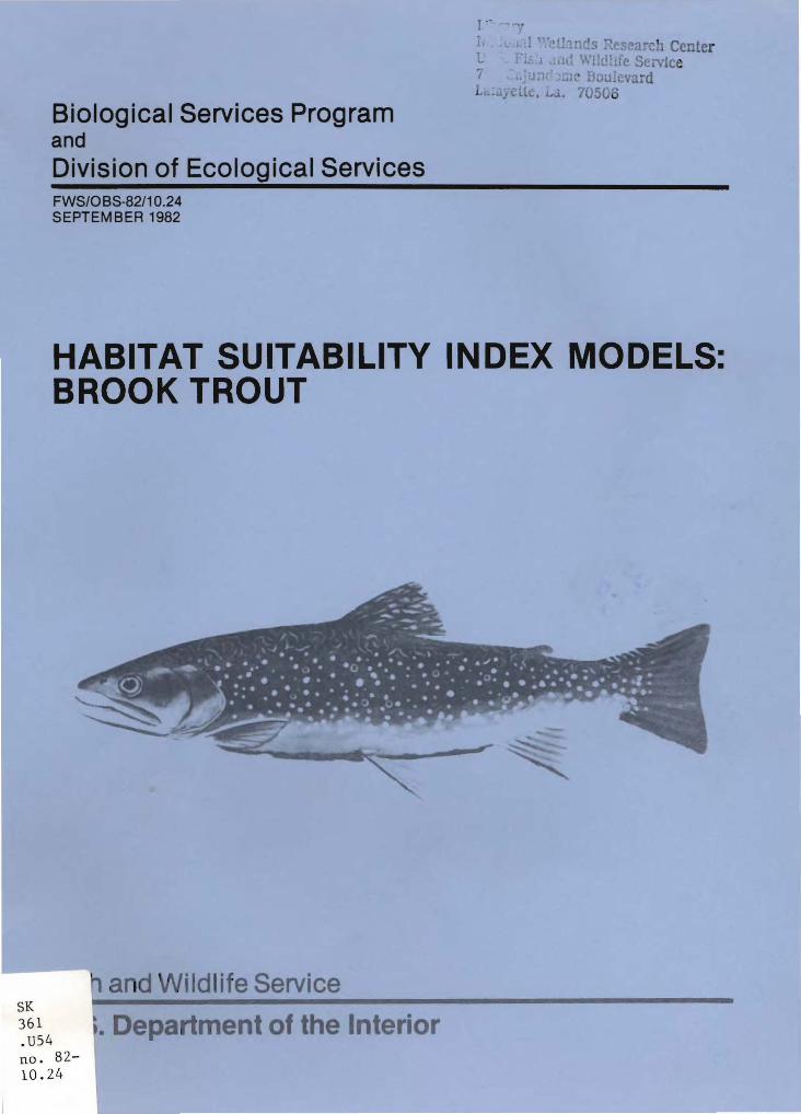
Tom Weshe, University of Wyoming; Robert Behnke, Colorado StateUniversity; Allan Binns, Wyoming Game and Fish Department; and Fred Eiserman,ETSI Pipeline Project provided a comprehensive review and many helpful commentsand suggestions on the manuscript. Charles Haines, Colorado Division ofWildlife, and Joan Trial, t,1aine Cooperative Fishery Unit, completed a litera­ture review to develop the report. Charles Solomon also reviewed the manu­script, provided comments, and prepared the final manuscript for publication.Cathy Short conducted the editorial review, and word processing was providedby Dora Ibarra and Carolyn Gulzow. The cover illustration is from FreshwaterFishes of Canada, Bulletin 184, Fisheries Research Board of Canada, byW. B. Scott and E. J. Crossman.

vi

BROOK TROUT (Salvelinus fontinalis)

HABITAT USE INFORMATION

General

The native range of brook trout (Salvelinus fontinalis Mitchill) orig­inally covered the eastern two-fifths of Canada northward to the Arctic Circle,the New England States, and southward through Pennsylvania, along the crest ofthe Appalachian Mountains to northeastern Georgia. Western limits includedManitoba southward through the Great Lake States. Reductions in the originalrange have resulted from environmental changes, such as pollution, siltation,and stream warming due to deforestation (MacCrimmon and Campbell 1969).

Si nee the 1ate 19th century, brook trout have been introduced into 20additional States and have sustaining populations in 14 States (MacCrimmon andCampbe11 1969). Introductions have not been attempted inmost of the centra 1plains and the southern States.

Brook trout can be separated into two basic ecological forms: a short­lived (3-4 years), small (200-250 mm) form, typical of small, cold stream andlake habitats and a long-lived (8-10 years), large (4-6 kg), predaceous formassociated with large lakes, rivers, and estuaries. The smaller, shor-t r l ivedform is typically found south of the Great Lakes region and south of northernNew England, while the larger form is located in the northern portion of itsnative range (Behnke 1980). Although no subspecies designation has beenrecogni zed for these two forms, they respond as two different speci es toenvironmental interactions influencing life history (Flick and Webster 1976;Flick 1977).

Brook trout can be hybridized artificially with lake trout (to produce afertile hybrid called splake trout) and with rainbow trout (Buss and Wright1957). In rare cases, natural hybrids occur between brook trout and browntrout (Salmo trutta); the hybrid is termed tiger trout (Behnke 1980). Behnke(1980) also collected brook trout and bull trout (Salvelinus confluentis)hybrids in the upper Klamath Lake basin, Oregon. Brook trout appear to besensitive to introductions of brown and rainbow trout and are usually displacedby them. However, brook trout have displaced cutthroat trout and grayling inheadwaters and tributaries of western streams (Webster 1975).

1

Age, Growth, and Food

Brook trout appear to be opportunistic sight feeders, utilizing bothbottom-dwelling and drifting aquatic macroinvertebrates and terrestrial insects(Needham 1930; Dineen 1951; Wiseman 1951; Benson 1953; Reed and Bear 1966).Such feeding habits make them particularly susceptible to even moderate tur­bidity levels, which can reduce their ability to locate food (Bachman 1958;Herbert et al. 1961a, 1961b; Tebo 1975). Drifting forms may be selected overbenthic forms when they are available (Hunt 1966). The choice of particulardrift organisms is apparently either a function of seasonal availabilityand/or the overall availability of terrestrial forms in a particular situation.Between age groups, there may be a tendency for selection of food items basedon size. In Idaho, age group 0 trout selected smaller drifting organisms(Diptera and Ephemeroptera) with less variation than did older trout, whileage group I trout seemed to prefer larger Trichoptera larvae (Griffith 1974).Fish are an important food item in lake populations (Webster 1975).

Reproduction

Age at sexual maturity varies among populations, with males usuallymaturing before females (Mullen 1958). Male brook trout may mature as earlyas age 0+ (Buss and McCreary 1960; Hunt 1966). In Wisconsin (Lawrence Creek),the smallest mature male was approximately 8.9 cm (3.5 inches) long (McFadden1961) .

Spawning typically occurs in the fall and has been described by severalauthors (Greeley 1932; Hazzard 1932; Smith 1941; Brasch et al. 1958, Needham1961). Spawning may begin as early as late summer in the northern part of therange and early winter in the southern part of the range (Sigler and Miller1963). The spawning behavior of brook trout is very similar to that of rainbowand cutthroat trout (Smith 1941). In streams and ponds, areas of ground waterupwelling appear to be highly preferred (Webster and Eiriksdottier 1976;Carline and Brynildson 1977) and to override substrate size as a site selectionfactor (Mullen 1958; Everhart 1966). Brook trout can be highly successfulspawners in lentic environments in upwelling areas of springs (Webster 1975).Spawning occurs at temperatures ranging from 4.5-10° C (White 1930; Hazzard1932; McAfee 1966). The fertilized ova are deposited in redds excavated bythe female in the stream gravels (Smith 1947). Spawning success is reduced asthe amount of fine sediments is increased and the intergravel oxygen concentra­tion is diminished (McFadden 1961; Peters 1965; Harshbarger 1975).

Migration and Anadromy

With the exception of the sea-run New England populations, brook troutmigrations are generally limited to movements into headwater streams or trib­utaries for spawning (Brasch et al. 1958) or relatively short seasonal migra­tions to avoid temperature extremes (Powers 1929; Scott and Crossman 1973).Some brook trout may spend their entire lives, including spawning periods,within a restricted stream area, as opposed "(.0 more migratory salmonids(McFadden et al. 1967). However, some movement upstream or downstream mayoccur due to space-related aggressive behavior following emergence from theredd (Hunt 1965).

2

· ...~

Some coastal populations of brook trout may move into salt water fromcoa sta 1 streams of ea stern Canada and northeastern Un i ted States. Sea-runindividuals caught in salt water may differ in appearance, form, and colorationfrom trout that have never or have not recently been in salt water (Smith andSaunders 1958). Not all brook trout in the same stream will necessarily moveto sea. In a study by White (1940), 79~~ of the brook trout going to sea wereage 2, and the rest were age 3. Smith and Saunders (1958) stated that age 1brook trout also migrated to the sea.

Smith and Saunders (1958) reported brook trout going to sea on PrinceEdward Island during spring and early summer and during fall and early winter.Movement was observed in every month of the year, although very few fish wereobserved migrating during midwinter and midsummer. Smith and Saunders (1958)observed that approximately half of the brook trout migrating to salt waterreturned to freshwater within a month. As temperatures decline in freshwater,brook trout tend to spend more time in saltwater, and some may overwinter insaltwater (Smith and Saunders 1958).

Specific Habitat Requirements

Brook trout are the most generalized and adaptable of all Salvelinusspecies. They inhabit small headwater streams, large rivers, ponds, and largelakes in inland and coastal areas. Typical brook trout habitat conditions arethose associated with a cold temperate climate, cool spring-fed ground water,and moderate precipitation (MacCrimmon and Campbell 1969). Warm water temper­atures appear to be the single most important factor limiting brook troutdistribution and production (Creaser 1930; Mullen 1958; McCormick et al.1972). In a comparative distribution study between brook and brown trout fromheadwater tributaries of the South Platte River, Colorado, Vincent and Miller(1969) found that, as the elevation increased and the streams became smallerand colder, brook trout became more abundant.

Optimal brook trout riverine habitat is characterized by clear, coldspri ng-fed water; a silt-free rocky substrate in riffl e-run areas; an approx­imate 1:1 pool-riffle ratio with areas of slow, deep water; well vegetatedstream banks; abundant instream cover; and relatively stable water flow,temperature regimes, and stream banks. Brook trout south of Canada tend tooccupy headwater stream areas, especi ally when ra i nbow and brown trout arepresent in the same river system (Webster 1975). They tend to inhabit largerivers in the northern portion of their native range (Behnke 1980).

Optimal lacustrine habitat is characterized as clear, cold lakes andponds that are typically oligotrophic. Brook trout are typically streamspawners, but spawning commonly occurs in gravels surrounding spring upwellingareas of lakes and ponds.

Cover is recognized as one of the basic and essential components of troutstreams. Boussu (1954) was able to increase the number and weight of trout instream sections by adding artificial brush cover and to decrease numbers andweight by removing brush cover and undercut banks. Lewi s (1969) found thatthe amount of cover present was important in determining the number of tro~

in sections of a Montana stream. Cover for trout consists of areas of low

3

stream bottom visibility, suitable water depths (> 15 cm), and low currentvelocity « 15 cm/s) (Wesche 1980). Cover can be provided by overhangingvegetation, submerged vegetation, undercut banks, instream objects (stumps,logs, roots, and large rocks), rocky substrate, depth, and water surfaceturbulence (Giger 1973). In a study to determine the amount of shade utilizedby brook, rainbow, and brown trout, Butler and Hawthorne (1968) reported thatrainbow trout showed the lowest preference for shade produced by artificialsurface cover. Brown trout showed the highest use of shade while brook troutwere intermediate between brown and rainbow trout. Brook trout in two Michiganstreams showed a strong preference for overhead cover along the stream margin(Enk 1977). The major limiting factor for brook trout in these streams wasbank cover.

Canopy cover is important in maintaining shade for stream temperaturecontrol and in providing allochthonous materials to the stream. Too muchshade, however, can restrict primary productivity in a stream. Stream temper­atures can be increased or decreased by controlling the amount of shade.About 50-75% midday shade appears optimal for most small trout streams(Anonymous 1979). Shading becomes less important as stream gradient and sizeincreases. In addition, a well vegetated riparian area helps to controlwatershed erosi on. In most cases, a buffer stri p about 30 m deep, 80~~ ofwhich is either well vegetated or has stable rocky stream banks, will provideadequate erosion control and maintain undercut stream banks characteristic ofgood trout habitat. The presence of fines in riffle-run areas can adverselyaffect embryo survival, food production, and cover for juveniles.

There is a definite relationship between the annual flow regime and thequality of trout habitat. The most critical) period is typically the base flow(lowest flows of late summer to winter). A base flow z 55% of the averageannual daily flow is considered excellent, a base flow of 25 to 50% is consid­ered fair, and a base flow of < 25% is considered poor for maintaining qualitytrout habitat (adapted from Wesche 1974; Binns and Eiserman 1979; Wesche1980) .

Hunt (1976) listed average depth, water volume, average depth of pools,amount of pool area, and amount of overhanging bank cover as the most importantparameters relating to brook trout carrying capacity in Lawrence Creek,Wisconsin. The main use of summer cover is probably for predator avoidanceand resting. Salmonids occupy different habitat areas in the winter than inthe summer (Hartman 1965; Everest 1969; Bustard and Narver 1975a).

In some streams, the major factor limiting salmonid densities may be theamount of adequate overwi nteri ng habi tat rather than summer reari ng habi tat(Bustard and Narver 1975a). Everest (1969) suggested that some salmonidpopulation levels were regulated by the availability of suitable overwinteringareas. Winter hiding behavior in salmonids is triggered by low temperatures(Chapman and Bjornn 1969; Everest 1969; Bustard and Narver 1975a,b). Bustardand Narver (1975a) indicated that, as water temperatures dropped to 4-80 C,feeding was reduced in young salmonids and most were found within or nearcover; few were more than 1 m from potential cover. Everest (1969) foundjuvenile rainbows 15-30 cm deep in the' substrate, which was often covered by5-10 cm of anchor ice. Lewis (1969) reported that adult rainbow trout tended

4

to move into deeper water during winter. The major advantages in seekingwinter cover are prevention of physical damage from ice scouring (Hartman1965; Chapman and Bjornn 1969) and conservation of energy (Chapman and Bjornn1969; Everest 1969). A cover area ~ 25% for adults and ~ 15% for juveniles ofthe entire stream habitat appears adequate for most brook trout populations.

Optimum turbidity val ues for brook trout growth are approximately 0-30JTU's, with a range of 0-130 JTU's (adapted from Sykora et al. 1972). Anaccelerated rate of sediment deposition in streams may reduce local brooktrout production because of the adverse effects on production of food organ­isms, smothering of eggs and embryos in the redd, and loss of escape andoverwintering habitat.

Brook trout appear to be more tolerant than other trout species to low pH(Dunson and Martin 1973; Webster 1975). Laboratory studies indicate thatbrook trout are tolerant of pH values of 3.5-9.8 (Daye and Garside 1975).Brook trout fingerlings in Pennsylvania inhabited a bog stream with a pH lessthan 4.75 and occassionally dropping to 4.0-4.2 (Dunson and Martin 1973).Parsons (1968) reported brook trout inhabiting a stream in Missouri with a pH'of 4.1-4.2. Creaser (1930) believed that brook trout tolerated pH rangesgreater than the range of most natural waters (4.1-9.5). Menendez (1976)demonstrated that continued exposure to a pH below 6.5 resulted in decreasedhatching and growth in brook trout. The selection of spawning sites may beassociated with the pH of upwelling water; neutral or alkaline waters (pH 6.7and 8) were selected by brook trout held at pH levels of 4.0, 4.5, and 5.0(Menendez 1976). The optimal pH range for brook trout appears to be 6.5-8.0,with a tolerance range of 4.0-9.5.

Brook trout occur in waters with a wide range of alkalinity and specificconductance, although high alkalinity and high specific conductance usuallyincrease brook trout production (Cooper and Scherer 1967). Brook trout popu­lations in the Smoky Mountains, North Carolina, are becoming increasinglyrestricted to low alkalinity headwater streams, apparently due to competitionfrom introduced rainbow trout (Salmo gairdneri), and are frequently in poorcondition (Lennon 1967). The small size of the trout in the headwater areashas been attributed to the infertility of the water, which has been linked tolow total alkalinities (10 ppm or less) and TDS values less than 20 ppm. TDSvalues in the Smoky Mountains are lower than values from similar streams inShenandoah National Park, Virginia, and the White Mountains National Forest,New Hampshire, where trout populations appear to be more robust.

Headwater trout streams are relatively unproductive. Most energy inputsto the stream are in the form of allochthonous materials, such as terrestrialvegetation and terrestrial insects (Idyll 1942; Chapman 1971; Hunt 1975).Aquatic invertebrates are most abundant and diverse in riffle areas withrubble substrate and on submerged aquatic vegetation (Hynes 1970). However,optimal substrate for maintenance of a diverse invertebrate population consistsof a mosaic of gravel, rubble, and boulders with rubble being dominant. Theinvertebrate fauna is much more abundant and diverse in riffles than in pools(Hynes 1970), but a ratio of about 1:1 of pool to riffle area (about 40-60%pool area) appears to provide an optimum mix of trout food producing and

5

rearing areas (Needham 1940). In riffle areas, the presence of fines (> 10~)

reduces the production of invertebrate fauna (based on Cordone and Kelly 1961;Platts 1974).

Adult. The reported upper and lOwer temperature limits for adult brooktrout vary; this may reflect local and regional population acclimation differ­ences. Bean (1909) reported that brook trout wi 11 not 1 i ve and thri ve intemperatures warmer than 20° C. McAfee (1966) indicated that brook troutusually do poorly in streams where water temperature exceeds 20° C for extendedperi ods. Brasch et. a 1 (1958) reported that brook trout exposed to tempera­tures of 25° C for more than a few hours did not surv i ve . Embody (1921)observed brook trout 1iving in temperatures of 24-27° C for short durationsand recommended 23.8° C as the maximum tolerable limit. Kendall (1924) agreedthat 23.9° C represented the 1imi t of even tempora ry endurance, but statedthat the optimum temperature should not exceed 15.6° C. Hynes (1970) statedthat brook trout can withstand temperatures from 0-25.3° C, but acclimation isnecessary. Th~ upper tolerable limit is raised by approximately 1° for every7° rise in acclimation temperature up to 18° C, where it levels off at theabsolute limit of 25.3° C. Fish kept at 24° C and above cannot toleratetemperatures as low as 0° C. Seasonal temperature cycles from summer highs towinter lows provide the necessary acclimation period needed to tolerate annualtemperature extremes. The overa 11 temperature range of 0-24° C was observedby MacCrimmon and Campbell (1969.

The above upper and lower tolerance limits probably do not reflect therange of temperatures that is most conducive to good growth. Baldwin (1951)cites an optimum growth rate at 14° C. He further contends that 11-16° C isbest suited for overall welfare, while trout exist at a relative disadvantagein terms of activity and growth at higher and lower, albeit tolerable, tempera­tures. Mullen (1958) gave the optimum temperature range for activity andfeeding for brook trout as between 12.8° C and 19° C. We assume that the tem­perature range for brook trout isO-24° C, wi th an optima 1 range for growthand survival of 11-16° C.

Brook trout normally require high oxygen concentrations with optimumconditions at dissolved oxygen concentrations near saturation and temperaturesabove 15° C. Local or temporal variations should not decrease to less than5 mg/l (Mills 1971). Dissolved oxygen requirements vary with age of fish,water temperature, water velocity, activity level, and concentration of sub­stances in the water (McKee and Wolf 1963). As temperatures increase, thedissolved oxygen saturation level in the water decreases, while the dissolvedoxygen requirements of the fish increases. As a result, an increase intemp8rature resulting in a decrease in dissolved oxygen can be detrimental tothe fish. Optimum oxygen levels for brook trout are not well documented butappear to be ~ 7 mg/l at temperatures < 15° C and ~ 9 mg/l at temperatures~ 15° C. Doudoroff and Shumway (1970) demonstrated that swimming speed andgrowth rates for salmonids declined with decreasing dissolved oxygen levels.In the summer (temperatures ~ 10° C), cutthroat trout generally avoid waterwith dissolved oxygen levels of less than 5 mg/l (Trojnar 1972; Sekulich1974). Fry (1951) stated that the lowest dissolved oxygen concentrations

6

where brook trout can exist is 0.9 ppm at 10° C and 1.6-1.8 ppm at 20° C.Embody (1927) contends that the dissolved oxygen concentration should not beless than 3 cc per liter (4.3 ppm).

E1 son (1939) reported that brook trout prefer moderate flows. Gri ffi th(1972) reported that focal point velocities for adult brook trout in Idahoranged from 7-11 em/sec, with a maximum of 25 em/sec. In a Wyoming study, 95%of all brook trout observed were associated with point velocities of less than15 em/sec (Wesche 1974).

The carrying capacity of adult brook trout in streams is dependent, atleast in part, on cover provided by pools, undercut banks, submerged brush andlogs, large rocks, and overhanging vegetation (Saunders and Smith 1955, 1962;Elwood and Waters 1969; O'Connor and Power 1976). Enk (1977) reported thatthe biomass and number of brook trout ~ 150 mm in size were significantlycorrelated with bank cover in two Michigan streams. Wesche (1980) reportedthat cover for adult trout should be located in stream areas with water depths~ 15 em and velocities of < 15 em/sec. We assume that an area ~ 25% of thetotal stream area occupied by brook trout will provide adequate cover.

Embryo. Temperatures in the range of 4.5-11.5° C have been reported asopt i mum for egg i ncubat ion (MacCri mmon and Campbell 1969). Length of eggincubation is about 45 days at 10° C, 165 days at 2.8° C (Brasch et al. 1958),and 28 days at 14.8° C (Embody 1934). Brook trout eggs develop slightlyfaster than brown trout eggs at 2° C or colder, but the reverse is true at3° C or above (Smith 1947). We assume that the range of acceptable tempera­tures for brook trout embryos is similar to that for cutthroat trout (Salmo~arki). --

Dissolved oxygen concentrations should not fall below 50% saturation inthe redd for embryo development (Harshbarger 1975). We assume that oxygenrequirements for embryos are similar to those of adults. Peters (1965) observ­ed high mortality rates when water velocity in the redd was reduced. Watervelocity is important in flushing out fines in the redds. Because brook troutcan successfully spawn in spawning areas of lakes, velocity is not necessaryfor successful spawning as long as oxygen levels are high and the redd is freeof silt. Spawning velocities for brook trout range from 1 em/sec (Smith 1973)to 92 em/sec (Thompson 1972; Hooper 1973). Spawning velocities measured forbrook trout in Wyoming ranged from 3-34 em/sec (Reiser and Wesche 1977).

Reiser and Wesche (1977) stated that optimum substrate size for brooktrout embryos ranges from 0.34-5.05 em. Duff (1980) reported a range ofsuitable spawning gravel size of 3-8 em in diameter for trout. Most workersagree that both water velocity and dissolved oxygen in the intergravel environ­ment determine the adequacy of the substrate for the hatching and survival ofsalmonid embryos and fry. Increases in sediment that alter gravel permeabil­ity reduces velocities and intergravel dissolved oxygen availability to theembryo and results in smothering of eggs (Tebo 1975). In a California study,brook trout survival was lower as the volume of materials less than 2.5 mm indiameter increased (Burns 1970). In a 30% sand and 70% gravel mixture, only28% of imp 1anted steel head embryos hatched; of those that hatched, on ly 74~~

7

emerged (Bjornn 1971; Phillips et al. 1975).gravel conditions include gravels 3-8 cmspawners) with ~ 5% fines.

We assume that suitable spawningin size (depending on size of

Fry. McCormick et al. (1972) cited temperature as an important limitingfactorof growth and di stri but i on of young brook trout. Fry emerge fromgravel redds from January to April, depending on the local temperature regime(Brasch et al. 1958). Temperatures from 9.8-15.4° C were considered suitable,with 12.4-15.4° C optimum; temperatures greater than 18° C were considereddetrimenta 1. The optimum temperature for brook trout fry, ina 1aboratorystudy, was between 8-12°C (Peterson et al. 1979). Upper lethal temperaturesare between 21 and 25.8° C (Brett 1940), possibly a reflection of differentacclimatization temperatures. Latta (1969) reported that upwelling groundwater was an important consideration for the well-being of fry in streams;Carline and Brynildson (1977) reported the same situation for fry in springponds. Menendez (1976) found that fry survival increased as pH increased from5 to 6.5. Griffith (1972) reported that focal point velocities for brooktrout fry in Idaho ranged from 8-10 cm/sec, with a maximum of 16 cm/sec.Because brook trout fry occupy the same stream reaches as adul ts, we assumethat temperature and dissolved oxygen requirements for brook trout fry aresimilar to those for adults.

Trout fry usually overwinter in shallow areas of low velocity, withrubble being the principal cover (Everest 1969; Bustard and Narver 1975a).Optimum size of substrate used as winter cover by steelhead fry and smalljuveniles ranges from 10-40 cm in diameter (Hartman 1965; Everest 1969). Arelatively silt-free area of substrate of this size class (10-40 cm), ~ 10% ofthe total habitat, will probably provide adequate cover for brook trout fryand small juveniles. The use of smaller diameter rocks for winter cover mayresult in increased mortal i ty due to shifting of the substrate (Bustard andNarver 1975a).

Juvenile. Davis (1961) stated that temperatures of 11-14° C are optimumfor fingerling growth. Griffith (1972) reported focal point velocities forjuvenile brook trout that ranged from 8.0-9.0 cm/sec, with a maximum of24 cm/sec. We assume that temperature and dissolved oxygen requirements forjuvenile brook trout are similar to those for adults.

Wesche (1980) reported that brook trout fry and small juveniles < 15 cmlong were associated more with instream cover objects (rubble substrate) thanoverhead stream bank cover. An area of cover ~ 15~~ of the total stream areaappears adequate for juvenile brook trout.

HABITAT SUITABILITY INDEX (HSI) MODELS

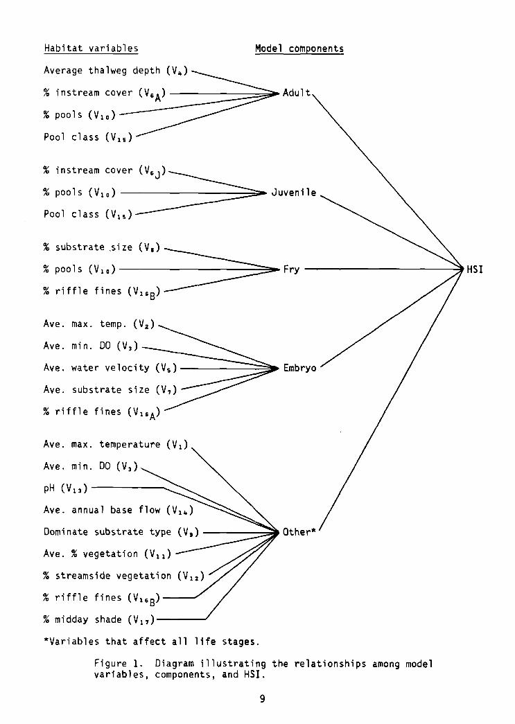
Figure 1 depicts the theoretical relationships among model variables,components, and HSI for the brook trout model.

8

Habitat variables Model components

Ave. max. temperature (V 1)

----""""'=~ Other""

Average thalweg depth

Ave. annual

Ave. min. DO (V 3 )

pH (V 13 ) -----........

Ave. % vegetation (V 11)

Ave. max. temp. (V 2 )

Ave. min. DO (V 3 )

Ave. substrate size

Ave. water velocity

Dominate substrate type

% instream cover (V&A) -----=::::::::::::::'~ Adult

% poo 1s (V 10 )

Pool class (V lS )

% riffl e fi nes

% riffle fines (Vl&B)-----~

% midday shade (V 17)------

% instream cover~(V&J)

% pools (V 10) ---------------- Juvenile

Pool class (V lS )

% substrate .size (V.)~

% pools (V 10) ~ Fry -----------~HSI

% riffle fines (V1&B)

% streamside vegetation

·Variables that affect all life stages.

Figure 1. Diagram illustrating the relationships among modelvariables, components, and HSI.

9

Model Applicability

Geographic area. The following model is applicable over the entire rangeof brook trout di stri but ion. Where differences in habitat requi rements havebeen identified for different races of brook trout, suitabil ity index graphshave been constructed to refl ect these di fferences. For thi s reason, caremust be excercised in use of the individual graphs and equations.

Season. The model rates the freshwater habitat of brook trout for allseasons of the year.

Cover types. The model is applicable to freshwater riverine or lacustrinehabitats.

Minimum habitat area. Minimum habitat area is the mlnlmum area of contig­uous habi tat that is requi red for a speci es to 1i ve and reproduce. Becausebrook trout can move considerable distances to spawn or locate suitable summeror winter rearing habitat, no attempt has been made to define a minimum habitatsize for the species.

Verification level. An acceptable level of performance for this brooktrout model is for it to produce an index between 0 and 1 that the authors andother biologists familiar with brook trout ecology believe is positivelycorrelated with the carrying capacity of the habitat. Model verificationconsisted of testing the model outputs from sample data sets developed by theauthor to simulate high, medium, and low quality brook trout habitat and modelreview by biologists familiar with brook trout ecology.

Model Description - Riverine

The riverine HSI model consists of five components: Adult (CA); Juvenile

(CJ ) ; Fry (C F); Embryo (C E); and Other (CO), Each life stage component con­

tai ns vari abl es specifi ca11y related to that component. The component Cocontains variables related to water quality and food supply that affect all1i fe stages of brook trout.

The model utilizes a modified limiting factor procedure. This procedureassumes that model variables and components with suitability indices in theaverage to good range, > 0.4 to < 1.0, can be compensated for by higher suit­ability indices of other, related model variables and components. However,variables and components with suitabilities s 0.4 cannot be compensated forand, thus, become limiting factors on habitat suitability.

Adult component. Variable V" percent instream cover, is included because

standing crops of adult trout have been shown to be correlated with the amountof cover available. Percent pools (V lD ) is included because pools provide

cover and resting areas for adult trout. Variable VlD also quantifies the

amount of pool habitat that is needed. Variable VB' pool class, is included

10

because pools differ in the amount and quality of escape cover, winter cover,and resting areas that they provide. Average thalweg depth (V4 ) is included

because average water depth affects the amount and qual ity of pool sandinstream cover available to adult trout and migratory access to spawning andrearing areas.

Juvenile component. Variables V6 , percent instream cover; VlO , percent

pools; and VIS' pool class are included in the juvenile component for the same

reasons listed above for the adult component. Juvenile brook trout use theseessential stream features for escape cover, winter cover, and resting areas.

Fry component. Variable Va, percent substrate size class, is included

because trout fry utilize substrate as escape cover and winter cover. VariableVlO , percent pools, is included because fry use the shallow, slow water areas

of pools and backwaters as resting and feeding stations. Variable V1 6 , percent

fines, is included because the percent fines affects the ability of the fry toutilize the rubble substrate for cover.

Embryo component. It is assumed that habitat suitability for troutembryos depends primarily on water temperature, V2 ; dissolved oxygen content,

V3 ; water velocity, Vs ; spawning gravel size, V7 ; and percent fines, V1 6 •

Water velocity, Vs ; gravel size, V7 ; and percent fines, V16 , are interrelated

factors that affect the transport of di ssol ved oxygen to the embryo and theremoval of the waste products of metabolism from the embryo. These functionshave been shown to be vital to the survival of trout embryos. In addition,the presence of too many fi nes in the redds wi11 block movement of the fryfrom the incubating gravels to the stream.

Other component. This component contains model variables for two subcom­ponents, water quality and food supply, that affect all life stages. Thesubcomponent water quality contains four variables: maximum temperature (VI);

minimum dissolved oxygen (V3 ) ; pH (V13 ) ; and base flow (V1 4 ) . All four vari­

ables affect the growth and survival of all life stages except embryo, whosewater quality requirements are included with the embryo component. The sub­component food supply contains three variables: substrate type (Vg ) ; percent

vegetation (Vll ) ; and percent fines (V1 6 ) . Dominant substrate type (Vg ) is

included because the abundance of aquatic insects, an important food item forbrook trout, is correlated with substrate type. Variable V16 , percent fines

in riffle-run and spawning areas, is included because the presence of excessivefines in riffle-run areas reduces the production of aquatic insects. VariableVll is included because allochthonous materials are an important source of

nutrients to cold, unproductive trout streams. The waterflow of all streamsfluctuate on an annual seasonal cycle. A correlation exists between the

11

average annual daily streamflow and the annual low base flow period in main­taining desirable stream habitat features for all life stages. Variable V1 4

is included to quantify the relationship between annual water flow fluctua­tions and trout habitat sUitability.

Variables VII' V1 2 , and V1 7 are optional variables to be used only when

needed and appropriate. Average percent vegetation for nutrient supply, VII'

should be used only on small « 50 m wide) streams with summer temperatures> 10° C. Percent streamside vegetation, V1 2 , is included because streamside

vegetation is an important means of controlling soil erosion, a major sourceof fines in streams. Variable Vl1 , percent midday shade, is included because

the amount of shade can affect water temperature and photosynthesis in streams.Variables Vll , V12 , and V1 7 are used primarily for streams 5 50 m wide with

temperature, photosynthesis, or erosion problems or when changes in theriparian vegetation is part of a potential project plan.

Suitability Index (SI) Graphs for Model Variables

This section contains suitability index graphs for 17 model variables.Equations and instructions for combining groups of variable SI scores intocomponent scores and component scores into brook trout HS1 scores are included.

The graphs were constructed by quantifying information on the effect ofeach habitat variable on the growth, survival, or biomass of brook trout. Thecurves were built on the assumption that increments of growth, survival, orbiomass originally plotted on the y-axis of the graph could be directly con­verted into an index of suitability from 0.0 to 1.0 for the species; 0.0 indi­cates unsuitable conditions and 1.0 indicates optimum conditions. Graph trendlines represent the aut.ho r l s best estimate of suitability for the variouslevels of each variable presented. The graphs have been reviewed by biologistsfamil i ar wi th the ecology of the speci es, but obvi ous ly some degree of 5Ivari abi 1i ty exi sts. The user is encouraged to vary the shape of the graphswhen existing regional information indicates a different variable suitabilityrelationship.

The habitat measurements and 51 graph construction are based on thepremise that extreme, rather than average, values of a variable most oftenlimit the carrying capacity of a habitat. Thus, measurement of extreme condi­tions, e.g., maximum temperatures and minimum dissolved oxygen levels, areoften the data used with the graphs to derive the 51 values for the model.The letters Rand L in the habitat column identify variables used to evaluateriverine (R) or lacustrine (L) habitats.

12

Habitat

R,L

Variable

Average maximum watertemperature (OC) duringthe warmest period ofthe year (adult,juvenile, and fry).

For lacustrine habitats,use temperature stratanearest optimum indissolved oxygen zonesof > 3 mg/l.

xQ)

'0 0.8c......

~ 0.6

~ 0.4+.J

='V"l 0.2

Suitability graph

+-_....-T'"""'"'......._"""'T-....._-lI~10 20 30

R Average maximum watertemperature (OC) duringembryo development.

1.0

x~ 0.8c......

~ 0.6

~ 0.4+.J

='V"l 0.2

R,L Average mlnlmum dissolvedoxygen (mg/l) during thelate growing season lowwater period and duringembryo development(adult, juvenile, fry,and embryo).

For lacustrine habitats,use the dissolved oxygenreadings in temperaturezones nearest to optimumwhere dissolvec oxygenis > 3 mg/l.

A = :s 15° CB = > 15° C

13

1.0

xQ)

0.8'0c......

~ 0.6'r--.-.Q 0.4ro+.J

=' 0.2V"l

3 6

I11g/1

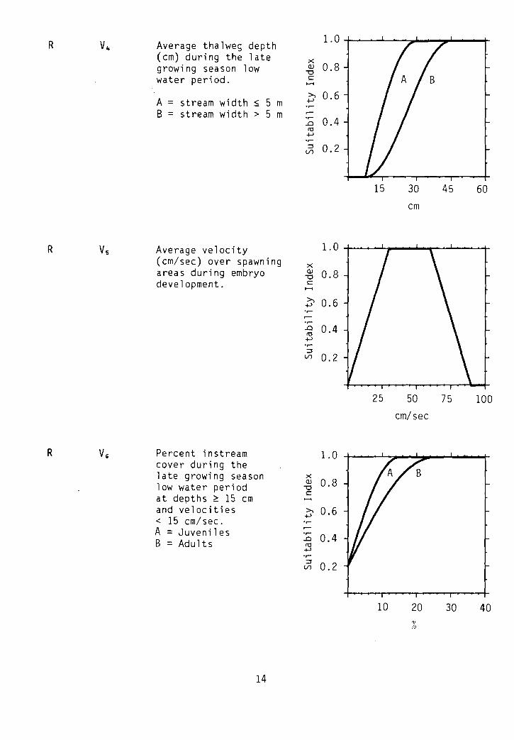
R V4 Average thalweg depth1.0

(em) during the late ><growing season low Q) 0.8

-0water period. c

.......>, 0.6

A = stream width s 5 m +->

B = stream width> 5 m..0 0.4co+->::::l 0.2(/)

15 30

em

45 60

R Vs Average ve1ocity 1.0(em/sec) over spawning ><areas during embryo Q) 0.8-0deve 1opment. c

.......>, 0.6+->

..0 0.4co+->::::l(/) 0.2

25 50

em/sec

75 100

R V, Percent instream 1.0cover during thelate growing season ><

Q) 0.8low water period -0c

at depths ~ 15 em .......

and velocities >, 0.615 em/sec. +->

<A Juveniles

.......= ......0.4B = Adults ..0

co+->::::l

0.2(/)

14

10 20

%

30 40

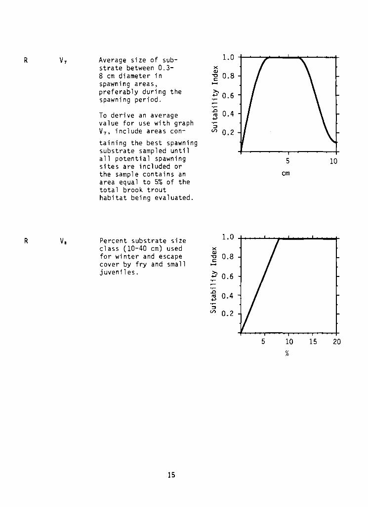
R V7 Average size of sub­strate between 0.3-8 cm diameter inspawning areas,preferably during thespawning period.

To derive an averagevalue for use with graphV7 , inciude areas con-

taining the best spawningsubstrate sampled untilall potential spawningsites are included orthe sample contains anarea equal to 5% of thetotal brook trouthabitat being evaluated.

1.0xQ)

0.8"0c:.-

~ 0.6...........c 0.4to.j-J.....~

(/') 0.2

5

em10

R V. Percent substrate size 1.0

class (10-40 cm) used xQ)

for winter and escape "0 0.8cover by fry and small c:.-juveniles. ~ 0.6.....

.....

.c0.4to

.j-J

~(/') 0.2

15

5 10

%

15 20

I

f-

f-

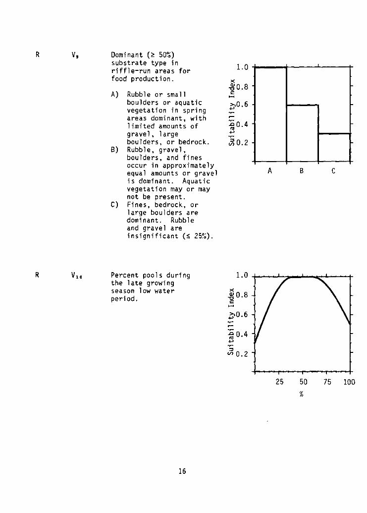
R Vg Dominant (~ 50%)substrate type in

1.0riffle-run areas forfood production. )(

~0.8A) Rubble or small c::....

boulders or aquatic ~0.6vegetation in spring ....areas dominant, with r-

limited amounts of ~0.4grave 1, large ~....boulders, or bedrock. ~ 0.2

B) Rubble, grave 1,boulders, and finesoccur in approximatelyequal amounts or gravelis dominant. Aquaticvegetation mayor maynot be present.

C) Fines, bedrock, orlarge boulders aredominant. Rubbleand gravel areinsignificant (s 25%).

A B c

R Percent pools duringthe late growingseason low waterperiod.

16

)(

~ 0.8c::....~0.6........~ 0.4~....='

V) 0.2

25 50

%

75 100

R Vll Average percent vege- 1.0

Optional tation (trees, shrubs, xand grasses-forbs) Q) 0.8""0

along the streambank c~

during the summer for >, 0.6allochthonous input. +J

'r-

Vegetation Index = r-.r-

2 (% shrubs) + 1.5 .0 0.4ro(% grasses) + (% trees) +J

'r-

+ 0 (% bareground). :;, 0.2V)

(For streams ~ 50 m wide)

1.0R V12

Optional

Average percent rootedvegetation and stable xrocky ground cover along ~ 0.8the streambank during the ~

summer (erosion control). >,+J 0.6'r-r-'r-.0

0.4ro.j-)

'r-:;,

V) 0.2

100

25

%

50

200

75

%

300

100

R,L Annual maximal orminimal pH. Use themeasurement with thelowest 51 value.

For lacustrine habitats,measure pH in the zonewith the best combina­tion of dissolvedoxygen and temperature.

1.0

x~ 0.8c~

~ 0.6r­'r-

~ 0.4+J'r-:;,

V) 0.2

17

4 5 678 9

pH10

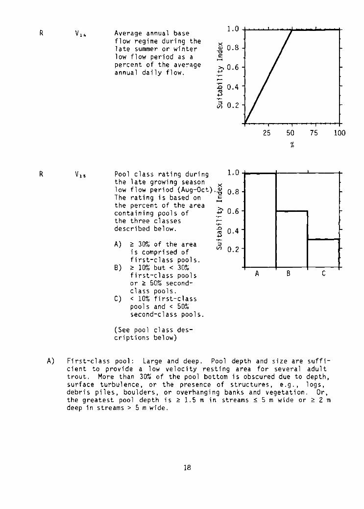
R Average annual baseflow regime during thelate summer or winterlow flow period as apercent of the ave~age

annual daily flow.

1. a +-................~-P-----t-

xOJ 0.8

"'0~......

~ 0.6-e--

:0 0.4<l:l~

~ 0.2

R V15 Pool class rating during 1.0the late growing season xlow flow period (Aug-Oct).~ 0.8The rating is based on ~

the percent of the area~ 0.6containing pools of

the three classes-e-

described below. .D 0.4<l:l~

I

I-

A) ~ 30% of the areais compri sed offirst-class pools.

8) ~ 10% but < 30%first-class poolsor ~ 50~~ second­class pools.

C) < 10% first-classpoo1sand < 50~~

second-class pools.

(See pool class des­criptions below)

-e-~

Vl 0.2

A

25 50

%

B

75

c

100

A) First-class pool: Large and deep. Pool depth and size are suffi­cient to provide a low velocity resting area for several adulttrout. More than 30% of the pool bottom is obscured due to depth,surface turbulence, or the presence of structures, e.g., logs,debris piles, boulders, or overhanging banks and vegetation. Or,the greatest pool depth is ~ 1.5 m in streams $ 5 m wide or ~ 2 mdeep in streams> 5 mwide.

18

B) Second-class pool: Moderate size and depth. Pool depth and sizeare sufficient to provide a low velocity resting area for a fewadult trout. From 5 to 30% of the bottom is obscured due to surfaceturbul ence, depth, or the presence of structures. Typi ca1 second­class pools are large eddies behind boulders and low velocity,moderately deep areas beneath overhanging banks and vegetation.

C) Third-class pool: Small or shallow or both. Pool depth and sizeare sufficient to provide a low velocity resting area for one tovery few adult trout. Cover, if present, is in the form of shade,surface turbulence, or very limited structures. Typical third-classpools are wide, shallow pool areas of streams or small eddies behindboulders.

R V16 Percent fines « 3 mm) 1.0in riffle-run and inspawning areas during x

OJ 0.8average summer f1 ows. "l::......

A = Spawning ?;> 0.6B = Riffle-run

.D 0.4ttl

.jJ

:;, 0.2Vl

15 30

%

45 60

R V17 Percent of stream area 1.0

Optional shaded between 1000 and x1400 hrs (for streams OJ 0.8

"::; 50 m wide). Do not l::......use on cold « 16° C ?;> 0.6max. temp. ), unproduc-tive streams.

''-.D 0.4ttl.jJ

:;,0.2Vl

19

25 50

%

75 100

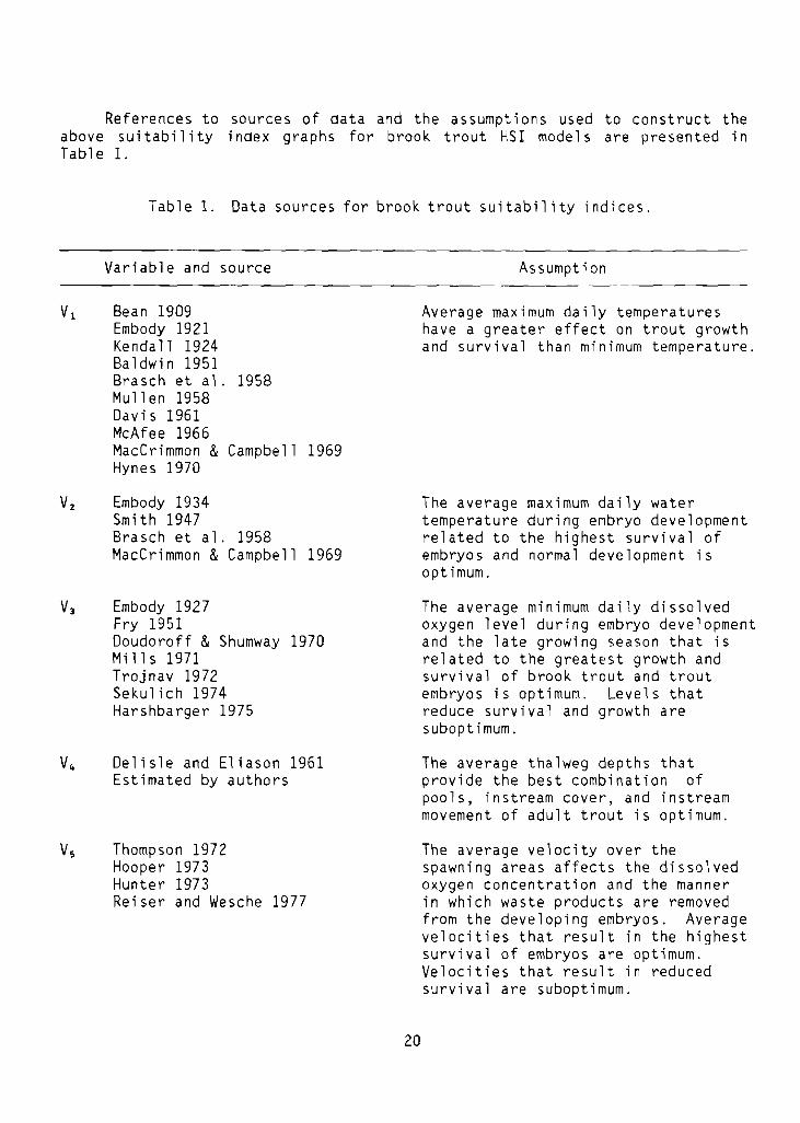
References to sources of data and the assumptions used to construct theabove sui tabi 1i ty index graphs for brook trout HSI mode 1s are presented inTable 1.

Table 1. Data sources for brook trout suitability indices.

Variable and source

Bean 1909Embody 1921Kendall 1924Baldwin 1951Brasch et al. 1958Mullen 1958Davis 1961McAfee 1966MacCrimmon &Campbell 1969Hynes 1970

Embody 1934Smith 1947Brasch et al. 1958MacCrimmon &Campbell 1969

Embody 1927Fry 1951Doudoroff & Shumway 1970Mills 1971Trojnav 1972Sekulich 1974Harshbarger 1975

Delisle and Eliason 1961Estimated by authors

Thompson 1972Hooper 1973Hunter 1973Reiser and Wesche 1977

Assumption

Average maximum daily temperatureshave a greater effect on trout growthand survival than minimum temperature.

The average maximum daily watertemperature during embryo developmentrelated to the highest survival ofembryos and normal development isoptimum.

The average minimum daily dissolvedoxygen level during embryo developmentand the late growing season that isrelated to the greatest growth andsurvival of brook trout and troutembryos is optimum. Levels thatreduce survival and growth aresuboptimum.

The average thalweg depths thatprovide the best combination ofpools, instream cover, and instreammovement of adult trout is optimum.

The average velocity over thespawning areas affects the dissolvedoxygen concentration and the mannerin which waste products are removedfrom the developing embryos. Averagevelocities that result in the highestsurvival of embryos are optimum.Velocities that result in reducedsurvival are suboptimum.

20

Variable and source

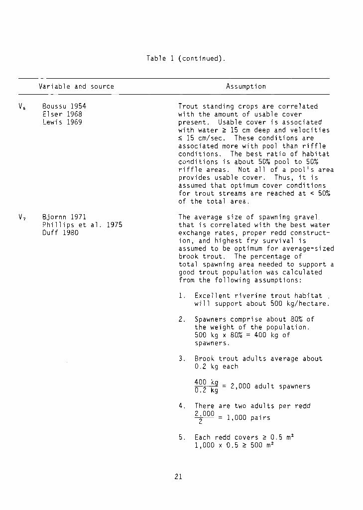
Boussu 1954Elser 1968Lewis 1969

Bjornn 1971Phillips et al. 1975Duff 1980

Table 1 (continued).

Assumption

Trout standing crops are correlatedwith the amount of usable coverpresent. Usable cover is associatedwith water ~ 15 em deep and velocities~ 15 em/sec. These conditions areassociated more with pool than riffleconditions. The best ratio of habitatconditions is about 50% pool to 50%riffle areas. Not all of a pool IS areaprovides usable cover. Thus, it isassumed that optimum cover conditionsfor trout streams are reached at < 50%of the total area.

The average size of spawning gravelthat is correlated with the best waterexchange rates, proper redd construct­ion, and highest fry survival isassumed to be optimum for average-sizedbrook trout. The percentage oftotal spawning area needed to support agood trout population was calculatedfrom the following assumptions:

1. Excellent riverine trout habitatwill support about 500 kg/hectare.

2. Spawners comprise about 80% ofthe weight of the population.500 kg x 80% = 400 kg ofspawners.

3. Brook trout adults average about0.2 kg each

400 kg = 2 000 adult0.2 kg' spawners

4. There are two adults per redd22000 = 1,000 pairs

5. Each redd covers ~ 0.5 m2

1,000 x 0.5 ~ 500 m2

21

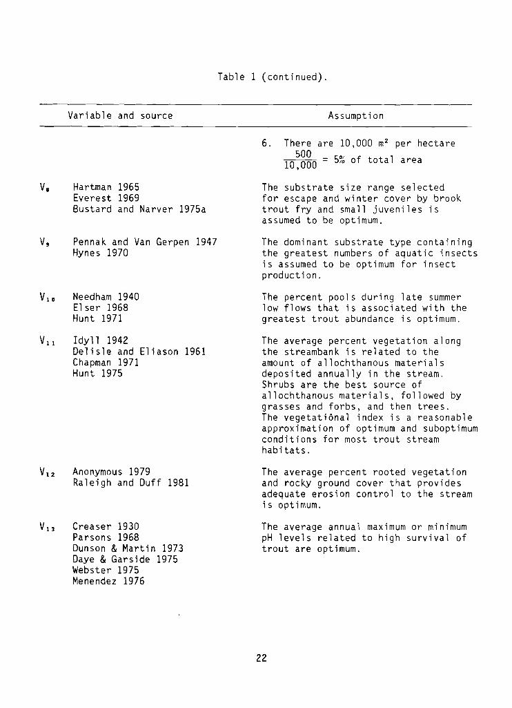
Table 1 (continued).

Variable and source Assumption

6. There are 10,000 m2 per hectare500 - 5~ f ttl10 000 - ~ 0 0 a area,

Hartman 1965Everest 1969Bustard and Narver 1975a

Pennak and Van Gerpen 1947Hynes 1970

Needham 1940Elser 1968Hunt 1971

Idyll 1942Delisle and Eliason 1961Chapman 1971Hunt 1975

Anonymous 1979Raleigh and Duff 1981

Creaser 1930Parsons 1968Dunson & Martin 1973Daye & Garside 1975Webster 1975Menendez 1976

The substrate size range selectedfor escape and winter cover by brooktrout fry and small juveniles isassumed to be optimum.

The dominant substrate type containingthe greatest numbers of aquatic insectsis assumed to be optimum for insectproduction.

The percent pools during late summerlow flows that is associated with thegreatest trout abundance is optimum.

The average percent vegetation alongthe streambank is related to theamount of allochthanous materialsdeposited annually in the stream.Shrubs are the best source ofallochthanous materials, followed bygrasses and forbs, and then trees.The vegetational index is a reasonableapproximation of optimum and suboptimumconditions for most trout streamhabitats.

The average percent rooted vegetationand rocky ground cover that providesadequate erosion control to the streamis optimum.

The average annual maximum or minimumpH levels related to high survival oftrout are optimum.

22

Variable and source

Binns 1979Adapted from Duff and

Cooper 1976

Needham 1940Lewis 1969Hunt 1976

Cordone & Kelly 1961Bjornn 1969Sykora et al. 1972Platts 1974Phi 11 ips et al. 1975

Sabean 1976, 1977Anonymous 1979

Table 1 (concluded).

Assumption

Flow variations affect the amount andquality of pools, instream cover, andwater quality. Average annual baseflows associated with the higheststanding crops are optimum.

Pool classes associated with thehighest standing crops of trout areoptimum.

The percent fines associated with thehighest standing crops of food organisms,embryos, and fry in each designated areais optimum.

The percent of stream area that isshaded that is associated with optimumwater temperatures and photosynthesisrates is optimum.

The above references include data from studies on related salmonid species.This information has been selectively used to supplement, verify, or completedata gaps on the habitat requirements of brook trout.

The suitability curves are a compilation of published and unpublishedinformation on brook trout. Information from other life stages or species orexpert opinion was used to formulate curves when data for a particular habitatparameter or life stage were insufficient. Data are not sufficient at thistime to refine the habitat suitability curves that accompany this narrative torefl ect subspecifi c or regi ona1 differences. Local knowl edge shoul d be usedto regionalize the suitability curves if that information will yield a moreprecise suitability index score. Additional information on this species thatcan be used to improve and regionalize the suitability curves should beforwarded to the Habitat Evaluation Group, U.S.D.I. Fish and Wildlife Service,2625 Redwing Road, Fort Collins, CO 80526.

23

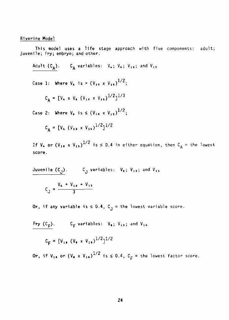
Riverine Model

This model uses a life stage approach with five components: adult;juvenile; fry; embryo; and other.

Case 2:

If V4 or (V1 0 x V1 s)l/2 is ~ 0.4 in either equation, then CA = the lowest

score.

Juvenile (CJ).

Or, if any variable is ~ 0.4, CJ = the lowest variable score.

Or, if V1 0 or (VI x V1 6)l/2 is ~ 0.4, CF = the lowest factor score.

24

Steps:

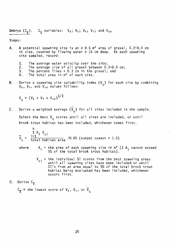
A. A potential spawning site is an ~ 0.5 m2 area of gravel, 0.3-8.0 cmin size, covered by flowing water ~ 15 cm deep. At each spawningsite sampled, record:

1. The average water velocity over the site;2. The average size of all gravel between 0.3-8.0 cm;3. The percent fines < 0.3 cm in the gravel; and4. The total area in m2 of each site.

B. Derive a spawning site suitability index (Vs) for each site by combiningVs , V7 , and V1 6 values follows:

/0.05 (output cannot> 1.0)areatotal habitat

C. Derive a weighted average (V s) for all sites included in the sample.

Select the best Vs scores until all sites are included, or until

brook trout habitat has been included, whichever comes first.

nr A. V .

i=l 1 S1

where Ai = the area of each spawning site in m2 (r A. cannot exceed5% of the total brook trout habitat). 1

V .S1

= the individual SI scores from the best spawning areasuntil all spawning sites have been included or untilSIrs from an area equal to 5% of the total brook trouthabitat being evaluated has been included, whicheveroccurs first.

D. Derive CE

CE = the lowest score of V2 , V3 , or Vs

25

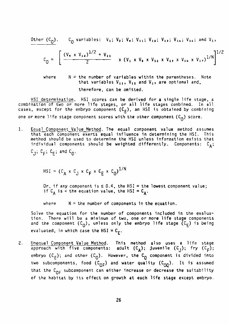
Other (CO) . Co variables: VI; VI; V,; VII; VIZ; VII; Vl~; V16 ; and V1 7

[ (V 9 x V16)l12

+ Vll r12liNC :: X (VI X VI X V12 X VII X Vl~ x V1 7 )0 2

where N =the number of variables within the parentheses. Notethat variables VII' VIZ and VI' are optional and,

therefore, can be omitted.

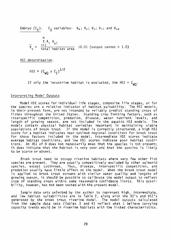
HSI determination. HSI scores can be derived for a single life stage, acombination of two or more life stages, or all life stages combined. In allcases, except for the embryo component (CE), an HSI is obtained by combining

one or more life stage component scores with the other component (CO) score.

1. Equal Component Value Method. The equal corr.ponent value method assumesthat each component exerts equal influence in determining the HSI. Thismethod should be used to determine the HSI unless information exists thatindividual components should be weighted differently. Components: CA;CJ ; CF; CE; and CO'

Or, if any component ;s s 0.4, the HSI ; the lowest component value;if CA ;s < the equation value, the HSI ; CA'

where N=the number of components in the equation.

Solve the equation for the number of components included in the evalua­tion. There will be a minimum of two, one or more life stage componentsand the component (CO), unless only the embryo lffe stage (C E) is being

evaluated, in which case the HSI =CEo

2. Unequal Component Value Method. This method also uses a life stageapproach with five components: adult (CA); juvenile (CJ ) ; fry (C F);embryo (CE); and other (CO), However, the Co component ;s divided into

two subcomponents, food (COF) and water quality (COQ)' It is assumed

that the COF subcomponent can either increase or decrease the suitability

of the habitat by its effect on growth at each life stage except embryo.

26

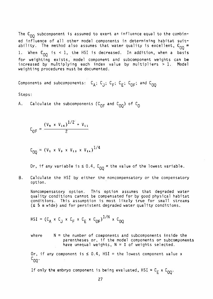
The COQ subcomponent is assumed to exert an influence equal to the combin­

ed i nfl uence of a11 other model components in determi ni ng habitat suit­ability. The method also assumes that water quality is excellent, COQ =1. When COQ is < I, the HSI is decreased. In addition, when a basis

for weighting exists, model component and subcomponent weights can beincreased by multiplying each index value by multipliers> 1. Modelweighting procedures must be documented.

Steps:

A. Calculate the subcomponents (COF and COQ) of Co

(V g x VI6) 1/ 2 + VIICOF = 2

Or, if any variable is ~ 0.4, COQ= the value of the lowest variable.

B, Calculate the HSI by either the noncompensatory or the compensatoryoption.

Noncompensatory option. This option assumes that degraded waterquality conditions cannot be compensated for by good physical habitatconditions. This assumption is most likely true for small streams(~ 5 mwide) and for persistent degraded water quality conditions.

HSI

where N = the number of components and subcomponents inside theparentheses or, if the model components or subcomponentshave unequal weights, N = L of weights selected.

Or, if any component is ~ 0.4, HSI = the lowest component value xCOQ'

If only the embryo component is being evaluated, HSI = CE x COQ'

27

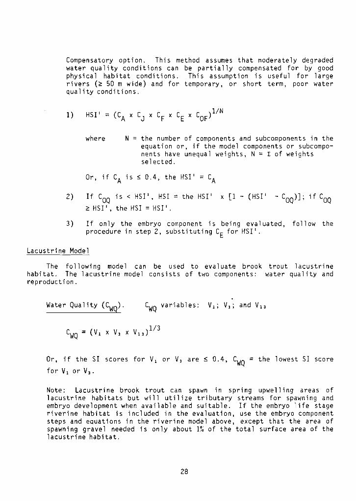
Compensatory option. This method assumes that moderately degradedwater quality conditions can be partially compensated for by goodphysical habitat conditions. This assumption is useful for largeri vers (~ 50 m wide) and for temporary, or short term, poor waterquality conditions.

where N = the number of components and subcomponents in theequation or, if the model components or subcompo­nents have unequal weights, N = L of weightsselected.

Or, if CA is ~ 0.4, the H5I' = CA

2) If COQ is < H5I ', H51 = the H5I ' x [1 - (H5I ' - COQ)]; if COQ

~ H5I ', the H5I = H5I '.

3) If only the embryo component is being evaluated, follow theprocedure in step 2, substituting CE for H5I'.

Lacustrine Model

The following model can be used to evaluate brook trout lacustrinehabitat. The lacustrine model consists of two components: water quality andreproduction.

Water Quality (CWQ)' CWQ va ria b1e s : V1; Vl; and V13

Or, if the 51 scores for V1 or Vl are s 0.4, CWQ = the lowest 51 score

for V1 or Vl •

Note: Lacustrine brook trout can spawn in spring upwell ing areas oflacustrine habitats but will utilize tributary streams for spawning andembryo development when available and suitable. If the embryo life stageriverine habitat is included in the evaluation, use the embryo componentsteps and equations in the riverine model above, except that the area ofspawning gravel needed is only about 1~~ of the total surface area of thelacustrine habitat.

28

nr A. V .

i=l 1 S1

total habitat area

HSI determination.

/0.01 (output cannot> 1.0)

HSI

If only the lacustrine habitat is evaluated, the HSI = CWQ'

Interpreting Model Outputs

Model HSI scores for individual life stages, composite life stages, or forthe species are a relative indicator of habt t.a t suitability. The HSI models,in their present form, are not intended to reliably predict standing crops offishes throughout the United States. Standing crop limiting factors, such asinterspecific competition, predation, disease, water nutrient levels, andlength of growing season, are not included in the aquatic HSI models. Themodels contain physical habitat variables important in maintaining viablepopulations of brook trout. If the model is correctly structured, a high HSIscore for a habitat indicates near optimum regional conditions for brook troutfor those factors included in the model, intermediate HSI scores indicateaverage habitat conditions, and low HSI scores indicate poor habitat condi­tions. An HSI of 0 does not necessarily mean that the species is not present;it does indicate that the habitat is very poor and that the species is likelyto be scarce or absent.

Brook trout tend to occupy ri veri ne habi tats where very few other fi shspecies are present. They are usually competitively excluded by other salmonidspecies, except cutthroat. Thus, disease, interspecific competition, andpredation usually have little affect on the model. When the brook trout modelis applied to brook trout streams with similar water quality and lengths ofgrowing season, it should be possible to calibrate the model output to reflectsize of standing crops within some reasonable confidence limits. This possi­bility, however, has not been tested with the present model.

Sample data sets selected by the author to represent high, intermediate,and low habitat suitabilities are in Table 2, along with the SIl s and HSI'sgenerated by the brook trout ri veri ne model. The model outputs ca 1cul atedfrom the sample data sets (Tables 3 and 4) reflect what I believe carryingcapacity trends would be in riverine habitats with the listed characteristics.

29

The models also have been reviewed by biologists familiar with brook troutecology; therefore, the model meets the previously specified acceptance level.

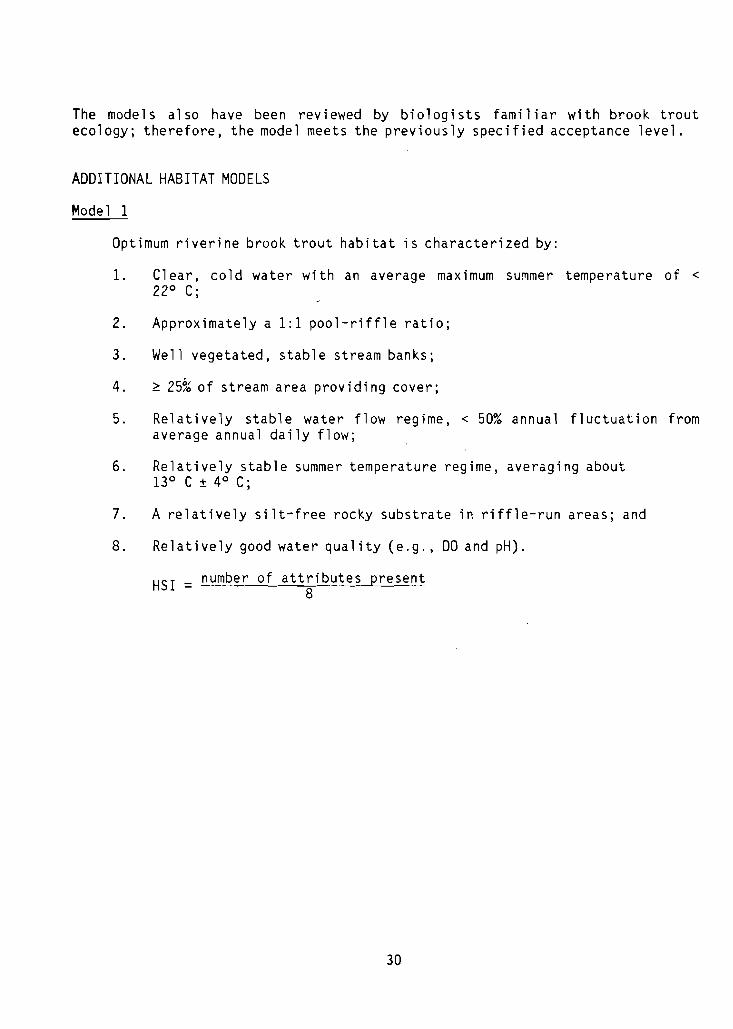
ADDITIONAL HABITAT MODELS

Model 1

Optimum riverine brook trout habitat is characterized by:

1. Cl ear, cold water with an average maximum summer temperature of <22° C;

2. Approximately a 1:1 pool-riffle ratio;

3. Well vegetated, stable stream banks;

4. ~ 25% of stream area providing cover;

5. Relatively stable water flow regime, < 50~~ annual fluctuation fromaverage annual daily flow;

6. Relatively stable summer temperature regime, averaging about13°C±4°C;

7. A relatively silt-free rocky substrate in riffle-run areas; and

8. Relatively good water quality (e.g., DO and pH).

HSI = number of attributes present8

30

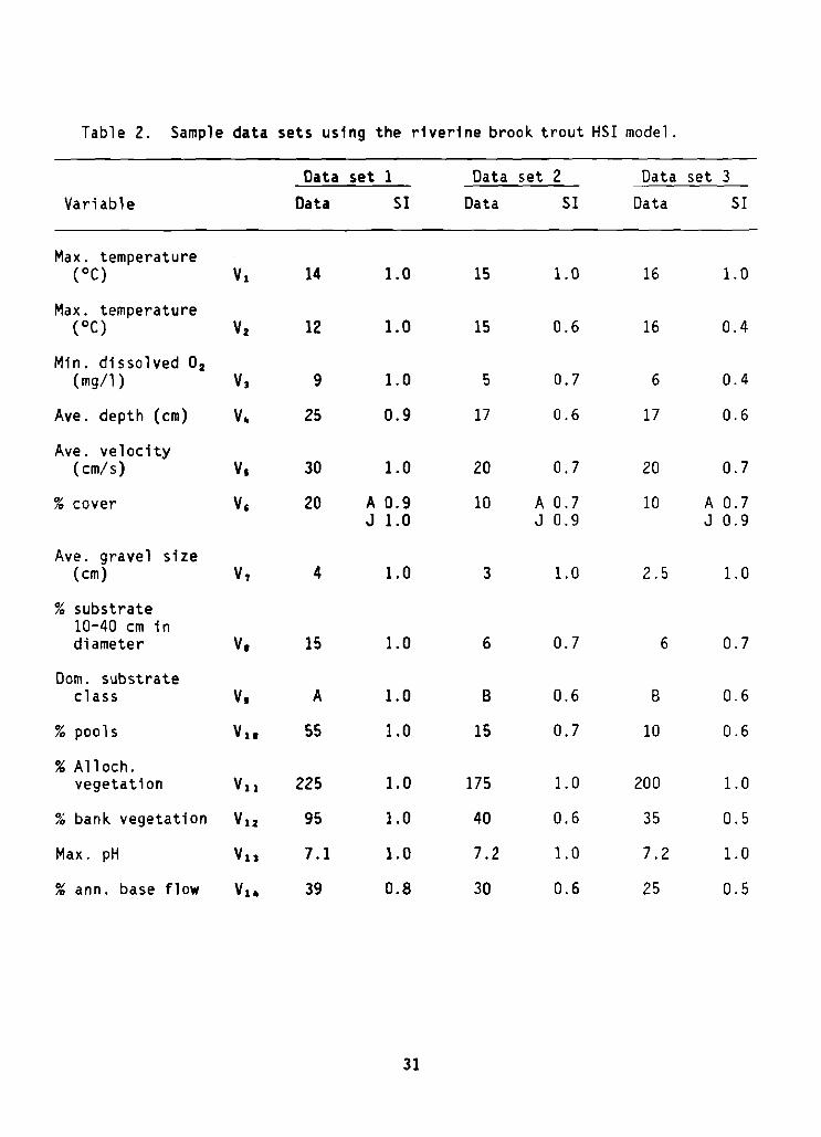
Table 2. Sample data sets using the riverine brook trout HSI model.

Data set 1 Data set 2 Data set 3

Variable Data SI Data SI Data SI

Max. temperature(OC) V1 14 1.0 15 1.0 16 1.0

Max. temperature(OC) V2 12 1.0 15 0.6 16 0.4

Min. dissolved O2(mg/l) V, 9 1.0 5 0.7 6 0.4

Ave. depth (cm) VII 25 0.9 17 0.6 17 0.6

Ave. velocity(em/s) VI 30 1.0 20 0.7 20 0.7

% cover V, 20 A 0.9 10 A 0.7 10 A 0.7J 1.0 J 0.9 J 0.9

Ave. gravel size(em) V, 4 1.0 3 1.0 2.5 1.0

% substrate10-40 em indiameter V. 15 1.0 6 0.7 6 0.7

Dom. substrateclass V, A 1.0 B 0.6 B 0.6

% pools VlI 55 1.0 15 0.7 10 0.6

% Alloeh.vegetation Vll 225 1.0 175 1.0 200 1.0

% bank vegetation V12 95 1.0 40 0.6 35 0.5

Max. pH Vu 7.1 1.0 7.2 1.0 7.2 1.0

~~ ann. base flow V110 39 0.8 30 0.6 25 0.5

31

Table 2. (concluded).

Data set 1 Data set 2 Data set 3

Variable Data 51 Data 51 Data 51

Pool class V15 A 1.0 B 0.6 C 0.3

°l fines (A) V16 5 1.0 20 0.4 20 0.4'0

% fines ( B) V16 20 0.9 35 0.6 35 0.6

°l shade V1 7 60 1.0 60 1.0 60 1.0,0

32

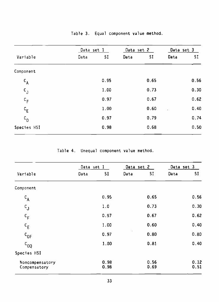
Table 3. Equal component value method.

Data set 1 Data set 2 Data set 3

Variable Data SI Data SI Data SI

Component

CA 0.95 0.65 0.56

CJ 1.00 0.73 0.30

CF 0.97 0.67 0.62

CE 1.00 0.60 0.40

Co 0.97 0.79 0.74

Species HS1 0.98 0.68 0.50

Table 4. Unequal component value method.

Data set 1 Data set 2 Data set 3

Variable Data SI Data SI Data SI

Component

CA 0.95 0.65 0.56

CJ 1.0 0.73 0.30

CF 0.97 0.67 0.62

CE 1.00 0.60 0.40

COF 0.97 0.80 0.80

COQ 1.00 0.81 0.40

Species HS1

Noncompensatory 0.98 0.56 0.12Compensatory 0.98 0.69 0.51

33

Model 2

A riverine trout habitat model has been developed by Binns and Eiserman(1979) Transpose the model output of pounds per acre to an index of 0-1:

HSI = model output of pounds per acreregional optimum pounds per acre

Model 3

Optimum lacustrine brook trout habitat is characterized by:

1. Clear, cold water with an average summer midepilimnion temperatureof < 22° C;

2. A midepilimnion pH of 6.5 to 8.5;

3. Dissolved oxygen content of epilimnion of ~ 8 mg/l; and

4. Presence of spring upwell ing areas or access to riverine spawningtributaries.

HSI = number of attributes present4

REFERENCES

Anonymous. 1979. Managing riparian ecosystems (zones) for fish and wildlifein eastern Oregon and eastern Washington. Prep. by the Riparian HabitatSubcommittee of the Oregon/Washington Interagency Wildl. Conf. 44 pp.

Bachman, R. W. 1958. The ecology of four north Idaho trout streams withreference to the influence of forest road construction. M.S. Thesis,Univ. of Idaho, Moscow. 97 pp.

Baldwin, N. S. 1951. A prel iminary study of brook trout food consumption andgrowth at different temperatures. Res. Council Ontario, 5th Tech.Session. 18 pp.

Bean, T. H. 1909. Examination of streams and lakes. 14th Ann. Rep. N.Y.State Forest, Fish and Game Comm., 1908. Pp. 215-217.

Behnke, R. J. 1980.Pages 441-480 inPubl.

A systematic review of theE. J. Balon, ed. Charr Monograph.

34

genus Sa lYe1i nus.The Hague: Junk.

Benson, N. G. 1953. Seasonal fluctuations in the feeding of brook trout inthe Pigeon River, Michigan. Trans. Am. Fish. Soc. 83:76-83.

Binns, N. A. 1979. A habitat quality index for Wyoming trout streams. Wyom.Game and Fish Dept. Fish. Res. Rep. 2. 75 pp.

Binns, N. A., and F.M. Eiserman. 1976. Environmental index of trout streams.Job 70 75-01-7101. Administrative files, Wyoming Game and Fish Dept.Cheyenne. 10 pp.

Binns, N. A., and F. M. Eiserman. 1979. Quantification of fluvial trouthabitat in Wyoming. Trans. Am. Fish. Soc. 108:215-228.

Bjornn, T. C. 1971. Trout and salmon movements in two Idaho streams asrelated to temperature, food, stream flow, cover, and population density.Am. Fish. Soc. Trans. 100(3):423-438.

Boussu, M. F. 1954. Relationship between trout populations and cover on asmall stream. J. Wildl. Manage. 18(2):229-239.

Brasch, J., J. McFadden, and S. Kmiotek. 1958. Brook trout.ecology, and management. Wise. Dept. Nat. Resour. Publ. 226.

Life hi story,15 pp.

Brett, J. R. 1940. Tempering versus acclimation in the planting of speckledtrout. Trans. Am. Fish. Soc. 70:397-403.

Burns, J. W. 1970. Spawning bed sedimentation studies in northern Californiastreams. California Fish Game 56(4):253-270.

Buss, K., and R. McCreary. 1960. A comparison of egg production of hatcheryreared brook, brown, and rainbow trout. Prog. Fish-Cult. 22(1):7-10.

Buss, K., and J. E. Wright. 1957. Results of species hybridization withinthe family Salmonidae. Prog. Fish-Cult. 18(4):149-158.

Bustard, D. R., and D. W. Narver. 1975a. Aspects of the winter ecology ofjuvenile coho salmon (Oncorhynchus kisutch) and steelhead trout (Salmogairdneri). J. Fish. Res. Board Can. 32(3):667-680.

__----;-:-_------;____._. 1975b. Preferences of j uven il e coho sa 1mon (Oncorhynchuskisutch) and cutthroat trout (Salmo clarki) relative to simulated altera­tion of winter habitat. J. Fish. Res. Board Can. 32(3):681-687.

Butler, R. L., and V. M. Hawthorne. 1968. The reactions of dominant trout tochanges in overhead artifical cover. Trans. Am. Fish. Soc. 97(1):37-41.

Carline, R. F., and O. M. Brynildson. 1977. Effects of hydraulic dredging onthe ecology of native trout populations in Wisconsin spring ponds. Dept.Nat. Resourc. Madison, WI. Tech. Bull. 98. 40 pp.

35

Chapman, D. W. 1971. The relative contribution of aquatic and terrestrialprimary producers to the trophic relation of stream organisms. Univ. ofPittsburg, Pymatuning Lab. of Ecol. Spec. Publ. 4:116-130.

Chapman, D. W., and T. C. Bjornn. 1969. Distribution of salmonids in streams,with special reference to food and feeding. Pages 153-176 in T. G.Northcote, ed. Symposium on salmon and trout in streams. H.R. MacMillianLec. in Fish. Univ. British Columbia, Vancouver.

Cooper, E. L., and R. C. Scherer. 1967. Annual production of brook trout(Salvelinus fontinalis) in fertile and infertile streams of Pennsylvania.Pa. Acad. Sci. Proc. 41:65-70.

Cordone, A. J., and D. W. Kelly. 1961. The influences of inorganic sedimentson the aquatic life of streams. California Fish Game 47(1):189-228.

Creaser, C. W. 1930. Relative importance of hydrogen-ion concentration,temperature, dissolved oxygen, and carbon-dioxide tension, on habitatselection by brook trout. Ecology 11(2):246-262.

Davis, H. S. 1961. Culture and diseases of game fishes. Univ. Calif. Press,Berkeley and Los Angeles, CA. 332 pp.

Daye, P. G., and E. T. Garside. 1975. Lethal levels of pH for brook trout,Salvelinus fontinalis. Can. J. Zool. 53(5):639-641.

Delisle, G. E., and B. E. Eliason. 1961. Effects on fish and wildliferesources of proposed water development on Middle Fork Feather River.State of Calif.-Oept. of Fish and Game Water Projects Rep. 19 pp.

Dineen, C. F. 1951. A comparative study of the food habits of Cottus bairdiand associated species of Salmonidae. Am. Midl. Nat. 46:640-645.

Doudoroff, P., and D. L. Shumway. 1970. Dissolved oxygen requirements offreshwater fishes. Food and Agriculture Organization of the UnitedNations, Rome. Fish. Tech. Paper 86. 291 pp.

Duff, D. A. 1980. Livestock grazing impacts on aquatic habitat in Big Creek,Utah. Paper presented at Livestock and Wildlife Fisheries Workshop.May 3-5, 1977. Reno, NV. U.S.D.l., Bur. Land Manage., Utah State Office.36 pp.

Duff, D. A., and J. Cooper. 1976. Techniques for conducting stream habitatsurveys on National Resource Lands. U.S.D.l., Bur. Land Manage. Tech.Note 283. 72 pp.

Dunson, W. A., and R. R. Martin. 1973. Survival of brook trout in a bog-derived acidity gradient. Ecology 54(6):1370-1376.

Elser, A. A. 1968.habi tat zones97(4):389-397

Fish populations of a trout stream in relation to majorand channel alterations. Trans. Am. Fish. Soc.

36

Elson, P. F. 1939. Effects of current on the movement of trout. J. Fish.Res. Board Can. 4(5):491-499.

Elwood, J. W., and T. F. Waters. 1969. Effects of floods on food consumptionand production rates of a stream brook trout population. Trans. Am.Fish. Soc. 98(2):253-262.

Embody, G. C. 1921. Concerning high water temperatures and trout. Trans.Am. Fish. Soc. 51 :58-64.

1927. An outline of stream study and the development of a stock­ing policy. Contrib. Agric. Lab., Cornell Univ. 54 pp.

1934. Relation of temperature to the incubation periods of eggsof four species of trout. Trans. Am. Fish. Soc. 64:281-291.

Enk, M. D. 1977. Instream overhead bank cover and trout abundance in twoMichigan streams. M.S. Thesis, Mich. State Univ., E. Lansing. 127 pp.

Everest, F. H. 1969. Habitat selection and spatial interaction of juvenilechinook salmon and steelhead trout in two Idaho streams. Ph.D. Diss.,Univ. Idaho, Moscow. 77 pp.

Everhart, W. H. 1966. Fishes of Maine. 3rd ed. Maine Dept. Inland Fish andGame. Augusta, ME. 96 pp.

Flick, W. A. 1977. Some observations, age, growth, food habits and vulner­ability of large brook trout ~Salvelinus fontinalis) from four CanadianLakes. Nature Canada 104(4):353-359.

Flick, W. A., and D. A. Webster. 1976. Production of wild, domestic, andinterstrain hybrids of brook trout (Salvelinus fontinalis) in naturalponds. J. Fish. Res. Board Can. 33(7):1525-1539.

Fry, F. E. 1951. Some environmental relations of the(Salveinus fontinalis). Northeast Atlantic Fish Conf.(Mimeo.).

speckled troutProc. 14 pp.

Garside, E. T. 1966. Effects of oxygen in relation to temperature on thedeve1opment of embryos of brook trout and rainbow trout. J. Fi sh. Res.Board Can. 23(8):1121-1134.

Giger, R. D. 1973. Streamflow requirements of salmonids. AFS-62-1. OregonWildl ife Comm., Portland. 117 pp.

Greeley, J. R. 1932. The spawning habits of brook, brown, and rainbow trout,and the problem of egg predators. Trans. Am. Fish. Soc. 62:239-247.

Griffith, J. S. 1972. Comparative behavior and habitat utilization of brooktrout (Salvelinus fontinalis) and cutthroat trout (Salmo clarki) in smallstreams in Northern Idaho. J. Fish. Res. Board Can. 29(3):265-273.

37

1974. Utilization of invertebrate drift by brook trout (Salvalinusfontinalis) and cutthroat trout (Salmo clarki) in small streams in Idaho.Trans. Am. Fish. Soc. 103(3):440-4~

Harshbarger, T. J. 1975. Factors affecting regional trout stream produc-tivity. Pages 11-27 in U.S.D.A. For. Servo Proc. Southeastern troutresource: ecology and management symposium. Southeastern Forest Exp.Stn., Asheville, NC. 145 pp.

Hartman, G. F. 1965. The role of behavior in the ecology and interaction ofunderyearling Coho salmon (Oncorhynchus kisutch) and steelhead trout(Salm~ gairdneri). J. Fish. Res. Board Can. 22(4):1035-1081.

Hazzard, A. S. 1932. Some phases in the life history of the eastern brooktrout, Salvelinus fontinalis, Mitchill. Trans. Am. Fish. Soc. 62:344-350.

Herbert, D. W. M., and J. C. Merken S. 1961. The effect of suspended mi nera 1solids on the survival of trout. Int. J. Air and Water Poll. 5:46-55.

Hooper, D. R.ecology.97 pp.

1973. Evaluation of the effects of flow on trout streamDept. Eng. Res., Pacific Gas and Electric Co. Emeryville, CA.

Hunt, R. L. 1965. Dispersal of wild brook trout during their first summer oflife. Trans. Am. Fish. Soc. 94(2):186-188.

1966. Production and angler harvest of wild brook trout inLawrence Creek, Wisconsin. Wisc. Div. Conserv., Madison. Tech. Bull. 35.52 pp.

1971. Responses of a brook trout population to habitat develop-ment in Lawrence Creek. Dept. Nat. Resourc., Madison, WI. Tech. Bull.48. 35 pp.

1976. In-stream improvement of trout habitat. Pages 26-31 inStream management of Salmonids. Trout Magazine, Pub. by Trout Unlimite~4260 East Evans, Denver, CO. 31 pp.

Hunter, J. W. 1973. A discussion of game fish in the State of Washington asre 1ated to water requi rements. Rep. from Fi sh Manage. Div., Wash. StateDept. Game, to Wash. State Dept. Ecol. 66 pp.

Hynes, H. B. N. 1970. The ecology of running waters. Univ. Toronto Press,Canada. 555 pp.

Kendall, W. C. 1924. The status of fish culture in our inland public watersand the role of investigation in the maintenance of fish resources.Roosevelt Wild Life Bull. 2(3):205-351.

38

Latta, W. C. 1969. Some factors affecting survival of young-of-the-yearbrook trout (Salve 1i nus font ina 1is, Mitchill) in streams. Pages 229-240in T. G. Northcoat, ed. The H. P. McMillon Lecture in Fisheries Senes.The Univ. Brit. Columbia Press. Vancouver, B.C. Feb. 22-24, 1968. 388pp.

Lennon, R. E. 1967. Brook trout of Great Smoky Mountains National Park.Bur. Sport. Fish. and Wildl. Tech. Paper 15. 18 pp.

Lewis, S. L. 1969. Physical factors influencing fish populations in pools ofa trout stream. Trans. Am. Fish. Soc. 98(1):14-19.

MacCrimmon, H. R., and J. C. Campbell. 1969. World distribution of brooktrout, Salvelinus fontinalis. J. Fish. Res. Board Can. 26:1699-1725.

McAfee, W. R. 1966. Eastern brook trout. Pages 242-260 in A. Calhoun, ed.Inland fisheries management. Calif. Dept. Fish Game.

McCormick, J. H., K. E. F. Hokansen, and B. R. Jones.temperature on growth and survival of young brookfontinalis. J. Fish. Res. Board Can. 29:1107-1112.

1972.trout,

Effects ofSalvelinus

McFadden, J. T. 1961. A population study of the brook trout, Salvelinusfontinalis. Wildl. Monogr. 7. 73 pp.

McFadden, J. T., G. R. Alexander, and D. S. Shetter. 1967. Numerical changesand population regulation in brook trout, Salvelinus fontinalis. J.Fish. Res. Board Can. 24:1425-1459.

McKee, J. E., and H.W. Wolf. 1963. Water quality criteria. State WaterControl Board. Sacramento, CA. Pub. 3A. 548 pp.

Menendez, R. 1976. Chr-cn i c effects of reduced pH on brook trout (Salvelinusfontinalis). J. Fish/Res. Board Can. 33(1)118-123.

Mills, D. 1971.management.

Salmon and trout; a resource, its ecology, conservation andSt. Martains Press, N.Y. 351 pp.

Mullen, J. W. 1958. A compendium of the life history and ecology of theeastern brook trout, Salvelinus fontinalis Mitchill. Mass. Div. FishGame, Fish. Bull. 23. 37 pp.

Needham, P. R. 1930. Studies on the seasonal food of brook trout. Trans.Am. Fish. Soc. 60:73-86.

1940. Trout streams. Comstock Pub1. Co., Ithaca, NY. 233 pp.

1961. Observations on the natural spawning of eastern brooktrout. California Fish Game 47(1):27-40.

O·Connor, J. F., and G. Power. 1976. Production by brook trout in the Matamekwatershed, Quebec. J. Fish Res. Board Can. 33(1):118-123.

39

Parsons, J. D. 1968. The effects of acid strip-mine effluents on the ecologyof a stream. Arch. Hydrobiol. 65:25-50.

Pennak, R. W., and E. D. VanGerpen. 1947. Bottom fauna production andphys i ca 1 nature of the substrate ina northern Colorado trout stream.Ecology 28(1):42-48.

Peters, J. C.surv i va 1 .Education275-279.

1965. The effects of stream sedimentation on trout embryoSeminar on Biol. Problems in Water Poll. U.S. Dept. Health.

and Welfare, Public Health Service, Cincinnati, OH. 1962. Pp.

Peterson, R. H., A. M. Sutterlin, and J. L. Metcalfe. 1979. Temperaturepreference of several species of Salmo and Salvelinus and some of theirhybrids. J. Fish. Res. Board Can. 36:1137-1140.

Phillips, R. W., R. L. Lantz, E. W. Claire, and J. R. Moring. 1975. Someeffects of gravel mixtures on emergence of coho sa 1mon and stee 1headtrout fry. Trans. Am. Fish. Soc. 3:461-466.

Platts, W. S. 1974. Geomorphic and aquatic conditions influencing salmonidsand stream classification with application to ecosystem classification.U.S.D.A., For. Serv., SEAM Pub1., Billings, MT. 199 pp.

Powers, E. B. 1929. Fresh water studies I. Ecology 10:97-111.

Rabe, F. W. 1967. The transplantation of brook trout in an alpine lake.Prog. Fish-Cult. 29(1):53-55.

Raleigh, R. F., and D. A. Duff. (in press).ment: eco logy and management. in W.Symposium II. Yellowstone Park, WY.

Trout stream habi tat i mprove­King, ed. Proc. Wild Trout

Reed, E. B., and G. Bear. 1966. Benthic animals and foods eaten by brooktrout in Archuleta Creek, Colorado. Hydrobiol. 27:227-237.

Reiser, D. W., and T. A. Wesche. 1977. Determination of physical andhydraulic preferences of brown and brook trout in the selection of spawn­ing locations. Water Resources Res. Inst., Univ. Wyo., Laramie. WaterRes. Series 64. 100 pp.

Rupp, R. S. 1953. The eastern brook trout, Salvelinus fontinalis (Mitchill)at Sunkhaze Stream, Maine. M.S. Thesis, Univ. Maine, Orono. 96 pp.

Sabean, B. 1976. The effects of shade removal on stream temperature in NovaSc~tia. Nova Scotia Dept. of Lands and Forests, Cat/76118/100. 32 pp.

Saunders, J. W., and M. W. Smith. 1955. Standing crop of trout in a smallPrince Edward Island stream. Can. Fish Cult. 17:32-39.

1962. Physical alterations of stream habitat to improve brooktrout production. Trans. Am. Fish. Soc. 91(2):185-188.

40

Scott, W. B., and E. J. Crossman. 1973. Freshwater fishes of Canada. Fish.Res. Board Can. Bull. 184. 966 pp.

Sekulich, P. T. 1974. Role of the Snake River cutthroat trout (Salmo clarkisubsp.) in fishery management. M.S. Thesis, Colo. State Univ.,Ft. Collins, CO. 102 pp.

Sigler, W. F. and R. R. Miller. 1963. Fishes of Utah. Utah Dept. Fish Game,Salt Lake City. 203 pp.

Smith, A. K. 1973. Development and application of spawning velocity anddepth criteria for Oregon salmonids. Trans. Am. Fish. Soc. 2:312-316.

Smith, M. W., and J. W. Saunders. 1958. Movements of brook trout, Salvelinusfont ina 1is between and withi n fresh and sa 1t water. J. Fi sh. Res. BoardCan. 15(6):1403-1449.

Smith, O. R. 1941. The spawning habits of cutthroat and eastern brook trouts.J. Wildl. Manage. 5(4):461-471.

1947. Returns from natural spawning of cutthroat trout andeastern brook trout. Trans. Am. Fish. Soc. 74:281-296.

Sykora, J., E. Smith, and M. Synak. 1972. Effect of lime neutralized ironhydroxide suspensions on juvenile brook trout (Salvelinus fontinalis,Mitchill). Water Res. 6:935-950.

)

1975. Review of selected parameters of trout stream quality.Pages 20-3l in Symposium on trout habitat research and management pro­ceedings. U:S.D.A., For. Serv., Southeastern For. Exp. Stn., Asheville,NC. 110 pp.

Thompson, K. 1972. Determining stream flows for fish life. Pages 31-50 inProc. Instream flow requirement workshop, Pacific Northwest River BasTilCommission, Vancouver, WA. Pp. 31-50.

Trojnar, J. R. 1972.cutthroat trout.59 pp.

Ecological evaluation of two sympatric strains ofM.S. Thesis, Colo. State Univ., Ft. Collins, CO.

Vincent, R. E., and W. H. Miller. 1969. Altitudinal distribution of browntrout and other fishes in a headwater tributary of the South PlatteRiver, Colorado. Ecology 50(3):464-466.

Webster, D. (Ed.) 1975. Proceedings of brook trout seminar. Wise. Dept.Nat. Resour., Univ. Wise. 16 pp.

Webster, D., and Eiriksdottier. 1976. Upwelling water as a factor influ-encing choice of spawning sites by brook trout (Salvelinus fontinalis).Trans. Am. Fish. Soc. 75:257-266.

41

Wesche, T. A. 1973. Parametic determination of mlnlmum streamflow for trout.Water Resour. Series 37. Water Resour. Res. Inst., Univ. of Wyom.,l.ar-amt e, WY. 102 pp.\

Wesch-e, T. A. 1974. Evaluation of trout cover in smaller streams. Proc.Western Assoc. Game and Fish Commissioners. 54:286-294.

. 1980. The WRRI trout cover rating method: developments and-----;---0-

application. Water Resour. Res. Inst., Water Resour. Ser. 78. 46 pp.

White, H. C. 1930. Some observations on the eastern brook trout (Salvelinusfontinalis) of Prince Edward Island. Trans. Am. Fish. Soc. 60:101-108.

. 1940. Life history of sea-running brook trout (Sa1velinus----=----c-fontinalis) of Moser River, N.S. J. Fish. Res. Board Can. 5(2):176-186.

Wiseman, J. S. 1951. A quantitative analysis of foods eaten by eastern brooktrout. Wyo. Wildl. 15:12-17.

42

50272 -retREPORT DOCUMENTATION

PAGE4. Title and Subtitle

7•..:4-ue'0 r(S) F R 1 . hKOuert . a elg

: 1. REPORT NO.

~ - FWSjOBS-82jl 0.24

Brook Trout

I 3. Recillient's Acc..sio" No.

i

I 14.II

15. SUlllllementary Notes

. IlL Abstract (LimIt: 200 words)

Habi tat Eva1ua t t on Procedures l)roup 110. Project/Tuk/Worlc Unit No.

U.S. Fish and Wildl ife Service f------------lWes tern Energy and Land Use Team 111. Contl'llet(C) or Grant(G) No.

Drake Creekside Building One : (C)

2625 Redwi ng Road IFort Collins, CO 80526 ~)

Western Energy and Land Use Team 13. l'YIM of Reoon &. Period Covered

Office of Biological ServicesFish and Wildlife ServiceU.S. Department of the InteriorWashington, DC 20240

Literature describing the habitat preferences of the brook trout (Salvelinus fontinalis)is reviewed, and the relationships between habitat variables and life requisites aresynthesized into a Habitat Suitability Index (HSI) model. HSI models are designedfor use with the Habitat Evaluation Procedures (HEP) in impact assessment and habitatmanagement activities.

I7A

Oqcume"f A"8'YSIS. a. Oescnlltonrn rna 1 benavtor

Aquatic biologyHabi tabil ityHabit

FishesTrout

:'. ld,"tlfiers/Ooe"·£nded l'ermsBrooK troutSalvelinus fontinalisHabitat Suitability Index (HSI)Habitat Evaluation Procedures (HEP)Impact assessment

c. COSAT! Field/Grauo

IS. Avallacllity Statement

RELEASE UNLIMITED

Habitat management

13. Securoty C:.~ss (ThIs .~eaart)

UNCLASSIFIED21. xe. of P'!iles

i; - vi +42pp

:Se. ANSI-Z.:l9.! 31 S..e Instruerlons ~n ~~v.r,..

*U.S. GOVERNMENT PRINTINGOF'ICE:tl82-lIllO-e21 I 421

OPTIONAl. FOR" 272 ;J.-;7

..ormerly I'l T1S- 3S1:eoartm."t of Commerce

•

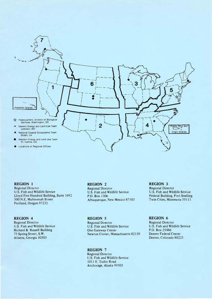
••• ..__ ....J~.

' .'· 0 ,,-

Hawaiian Islands (>

-(:( Headq uarters . Division of BiologicalServices, Wasnington, DC

x Eastern Energy anO Land Use TeamLeetown , WV

* Nationa l Coastal Ecosystems TeamSli dell , LA

• Western Energy and Land Use TeamFt. Coll ins . CO

• Locat ions of Regional Off ices

REGION 1Regional DirectorU,S. Fish and Wildlife ServiceLloyd Five Hundred Building, Suite 1692500 N.E. Multnomah StreetPortland , Oregon 97232

REGION 4Regional DirectorU.S. Fish and Wildlife ServiceRichard B. Russell Building75 Spring Street , S.W.Atlanta, Georgia 30303

IJ- - - ----

6 1r-- - -~-

L, JI : - ~- --I I

1- - -'I Il,_I 2 ,,-~--

-_.J

REGION 2Regional DirectorU.S. Fish and Wildlife ServiceP.O. Box 1306Albuquerque, New Mexico 87 103

REGION 5Regional DirectorU.S. Fish and Wildlife ServiceOne Gateway Cente rNewton Corner, Massachusetts 02158

REGION 7Regional DirectorU.S. Fish and Wildlife ServicelOll E. Tudor RoadAnchorage, Alaska 99503

- ..~,.

REGION 3Regional DirectorU.S. Fish and WildlifeServiceFederal Building, Fort SnellingTwin Cities, Minnesota 551 J I

REGION 6Regional DirectorU.S. Fish and Wildli fe ServiceP.O. Box 25486Denver Federal CenterDenver, Colorado 8022 5

u.s.FISH ..WILDLIFE

f>ERVICE

DEPARTMENT OF THE INTERIOR hi?]u.s.FISH ANDWILDLIFESERVICE ~

"'-r rw T " "

As the Nat ion's pri ncipal conservation agency, the Department of the Interior has respon­sibility for most of our ,nationally owned public lands and natural resources . This includesfostering the wisest use of our land and water resources, protecting our fish and wildlife,preserving th & environmental and cultural values of our national parks and historical places,and providing for the enjoyment of life through outdoor recreation. The Department as­sesses our energy and mineral resources and works to assure that t heir development is inthe best interests of all our people. The Department also has a major respons ibility forAmerican Indian reservation communit ies and for people who live in island territories underU.S. adm inist ration.