Habitat Occupancy and Movements by Greater Sage-Grouse …...Aldridge & Brigham 2003; Schroeder et...

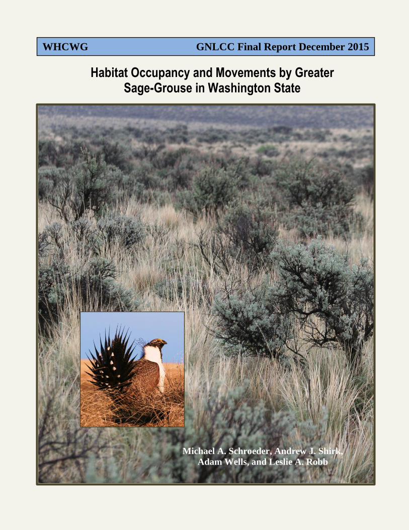
Habitat Occupancy and Movements by Greater Sage-Grouse in Washington State

WHCWG GNLCC Final Report December 2015

Michael A. Schroeder, Andrew J. Shirk,

Adam Wells, and Leslie A. Robb

ii

Cover photo of male Greater Sage-Grouse by Michael A. Schroeder. Title page and TOC page

illustrations by Brian Maxfield.

iii

Habitat Occupancy and Movements by Greater Sage-Grouse

in Washington State

December 2015

Michael A. Schroeder, Washington Department of Fish and Wildlife

P.O. Box 1077, Bridgeport, WA 98813

Andrew J. Shirk, University of Washington Climate Impacts Group

Box 355672, Seattle, WA 98195

Adam Wells, Washington State University, Vancouver, WA 98686

Leslie A. Robb, P.O. Box 1077, Bridgeport, WA 98813

Contact information: Michael A. Schroeder, 509-686-2692, [email protected]

mailto:[email protected]

iv

Acknowledgements

This project would not have been possible without the long-term data collected for Greater Sage-

Grouse by Washington Department of Fish and Wildlife field biologists and we thank the

numerous people who have contributed to this effort. We especially thank Jason Lowe (BLM)

for acquiring GPS transmitters and Mike Atamian (WDFW) for managing the GPS dataset.

Funding

This report builds upon connectivity models developed by the Washington Wildlife Habitat

Connectivity Working Group (WHCWG). In addition to funding provided by WHCWG

organizations the following entities provided additional support:

Bureau of Land Management

Department of Defense, Yakima Training Center

Great Northern Landscape Conservation Cooperative

Columbia Plateau Ecoregion. Photo by Joe Rocchio.

v

Table of Contents

Acknowledgements ........................................................................................................................ iv

Abstract .......................................................................................................................................... vi

Document Overview ....................................................................................................................... 1

Introduction ..................................................................................................................................... 1

Greater Sage-Grouse ................................................................................................................... 2

Habitat Associations .................................................................................................................... 4

Movements .................................................................................................................................. 6

Project Objectives ....................................................................................................................... 6

Overview of Data Used ............................................................................................................... 6

Objective 1: Species Distribution Modeling ................................................................................... 9

Introduction ................................................................................................................................. 9

Methods ....................................................................................................................................... 9

Results ......................................................................................................................................... 9

Discussion ................................................................................................................................. 10

Objective 2: Movement Modeling ................................................................................................ 17

Introduction ............................................................................................................................... 17

Methods ..................................................................................................................................... 17

Results ....................................................................................................................................... 18

Discussion ................................................................................................................................. 20

Future Direction ........................................................................................................................ 22

Literature Cited ............................................................................................................................. 29

Presentations ................................................................................................................................. 33

vi

Abstract

Local extirpations drive species’ range contractions, and are often precursors of extinction.

Understanding the dynamics underlying these processes is critical for devising effective

conservation strategies. The Greater Sage-Grouse (Centrocercus urophasianus) is an example of

a species undergoing range contraction, with local extirpations occurring over nearly half of the

historically occupied habitat. The Columbia Basin population in Washington State, USA, is

particularly threatened, as it persists in a highly modified agricultural landscape that other studies

have characterized as similar to extirpated range. Yet declines in this population have stabilized,

and unoccupied habitat is being successfully recolonized via translocations. In this study, we

used species distribution modeling to quantify environmental variables constraining sage grouse

distribution in Washington, with the primary objective to understand how this species may

persist in agricultural landscapes. We also used GPS location data collected from translocated

birds to understand how natural and anthropogenic features of the landscape influence movement

patterns. We found that fields planted to perennial vegetation as part of the Conservation Reserve

Program (CRP) are critical in providing year-round habitat for sage grouse (and likely many

other species) when intermixed with native sagebrush. Without this program, we estimate 63%

of sage grouse habitat in Washington would become unsuitable. Conversely, if CRP allotments

were redistributed to better support sage grouse, we estimate the area of habitat could be

increased by 66%. In addition to the area of native sagebrush and CRP lands, we also found that

climate variability, the patch configuration of sagebrush, and development impacts constrain the

distribution within the study area. With careful consideration of the multiple intended uses of the

program, it may be possible to strategically allocate a portion of CRP allowances over space and

time to reduce the risk of extirpation in agricultural areas, and to facilitate sage grouse range

shifts in response to climate-driven changes in the sagebrush biome. With regard to GPS data,

we did not find evidence that perception of the landscape, as represented by the alternative

resistance models, was different between early-mortalities and long-surviving sage grouse. A

close look at the statistically similar-top 4 movement models showed that the top-ranked model

was the null model. This suggested that the least-cost path is found in straight line from the first

GPS telemetry point to the last GPS telemetry point of each 5 km path. This process illustrated

some potential approaches for future analysis.

This report, submitted by the Washington Connected Landscapes Project, is the Final Report

for Informing Connectivity Conservation Decisions for Greater Sage-Grouse in the

Columbia Plateau Ecoregion deliverables outlined in Agreement number F14AP01042 with

the United States Fish and Wildlife Service.

December 2015 GNLCC FINAL REPORT

Connectivity Conservation for Greater Sage-Grouse in Washington 1

Document Overview

This report presents results for the development of a habitat model for Greater Sage-Grouse

(Centrocercus urophasianus) in Washington State and an analysis of movements by GPS-

collared translocated birds. Spatial data layers used in the analyses and supporting information

are freely available from http://www.waconnected.org. This document is organized as follows:

1) Introduction—Background information about conservation of sage grouse in the region,

habitat associations and movements for Greater Sage-Grouse in Washington State,

project objectives, and an overview of Greater Sage-Grouse data used in the analyses.

2) Species distribution modeling—An assessment of landscape factors associated with the

presence of sage grouse in the Columbia Basin of Washington State. We also considered

seasonal differences in sage grouse responses to environmental variables, as well as the

spatial scale at which these variables were important predictors of occurrence.

3) Movement modeling—The findings and recommendations of the analysis of existing

landscape resistance surfaces in conjunction with GPS data acquired from translocated

sage-grouse.

4) Literature cited and Presentations

Introduction

The Washington Wildlife Habitat Connectivity Working Group (WHCWG) has produced

detailed connectivity analyses for the 20 million acre Columbia Plateau, a sage shrub/grassland

(WHCWG 2012, 2013). Whereas agriculture and infrastructure dominate the human footprint of

the Columbia Plateau Ecoregion, understanding the functional wildlife habitat connectivity in

this highly fragmented landscape is in early stages.

Empirical validation of the WHCWG Columbia Plateau sage-grouse resistance model (Shirk et

al. 2015) showed that transmission lines convey a stronger impact to landscape resistance than

originally predicted by the expert model. While the model testing assessed connectivity between

existing sage-grouse populations, it did not consider connectivity between existing populations

and unoccupied modeled suitable habitat, i.e., potential translocation sites. This is because range-

wide habitat models perform poorly in Washington at predicting presence and absence of sage-

grouse (Aldridge et al. 2008; Wisdom et al. 2011; Knick et al. 2013). The poor fit of range-wide

models for sage-grouse in the Columbia Plateau has important implications for conservation of

this species, limiting management objectives in Washington (Stinson et al. 2004).

The Washington Department of Fish and Wildlife (WDFW) in cooperation with the USFWS

have been conducting a translocation effort since 2008 to establish a population of Greater Sage-

Grouse on the Swanson Lakes Wildlife Area (Schroeder et al. 2013). In 2014, 20 GPS radio

transmitters were provided by the Bureau of Land Management (BLM) to monitor translocated

birds. Species based connectivity models make fundamental assumptions as to how animals

perceive and move through the landscape. For instance, even though we often record dispersal

movements as straight-line distances, we know that species make pathway decisions influenced

http://www.waconnected.org/



by habitat resistance. Understanding patterns of movement through the landscape and the factors

that influence movement pathways is important for conservation efforts that address habitat and

population connectivity. Translocated birds make exploratory movements within the first few

weeks after release. These movements are analogous to dispersal movements and provide the

unique opportunity to gain insight as to how sage-grouse perceive natural and anthropogenic

(e.g., powerlines, roads, croplands, areas impacted by wildfire) landscape features.

Greater Sage-Grouse

Greater Sage-Grouse are considered a landscape species for shrubsteppe ecosystems (Hanser &

Knick 2011). They have large home ranges, are capable of extensive movements, and use a

mosaic of habitat patch sizes (Connelly et al. 2004). Greater Sage-Grouse are sensitive to

disturbance from human activities as well as the configuration and juxtaposition of suitable

habitat in the landscape (Braun 1986; Lyon & Anderson 2003; Connelly et al. 2004; Aldridge

2005; Aldridge & Boyce 2007; Holloran et al. 2010; Johnson et al. 2011; Knick & Hanser 2011;

Wisdom et al. 2011). Habitat loss, degradation, and fragmentation of native shrubsteppe

vegetation resulting from altered fire regimes, conversion of shrubsteppe to agriculture, urban

development, energy development, grazing, mining, military activity, noise, powerlines, roads,

fences, and encroachment by invasive plant species threaten the persistence of populations in

Washington (Schroeder et al. 2003; Stinson et al. 2004). Additional threats include loss of

genetic diversity through population isolation (Stinson et al. 2004) and evidence suggests that

Greater Sage-Grouse in Washington have already undergone a genetic bottleneck (Benedict et al.

2003; Oyler-McCance et al. 2005; Oyler-McCance & Quinn 2011).

Greater Sage-Grouse were once widely distributed throughout central and eastern Washington,

parts of north-central and eastern Oregon, southern Idaho and in the extreme southern portion of

British Columbia following the Okanagan valley (Campbell et al. 1990; Schroeder et al. 2000;

Aldridge & Brigham 2003; Schroeder et al. 2004). Initial declines of Greater Sage-Grouse

distribution in Washington were related to cultivation of shrubsteppe habitat, primarily for

production of wheat, and continued as cultivation expanded throughout the Columbia Basin

(Schroeder et al. 2000). The estimated range of Greater Sage-Grouse in Washington is

approximately 4683 km2 or 8% of the historical range (Schroeder et al. 2000). Current estimates

place the state population at approximately 1000 birds (2015 estimate; MAS).

There are two endemic populations of Greater Sage-Grouse in Washington (Fig. 1). One is

located in the Moses Coulee area in Douglas/Grant counties and one is on the U.S. Army’s

Yakima Training Center (YTC) in Yakima/Kittitas counties (Schroeder et al. 2000; Stinson et al.

2004). These populations are isolated from each other by approximately 50 km and from

populations in Oregon and Idaho by about 250 km and 350 km respectively. In 2008 WDFW

initiated a translocation project to release birds at the Swanson Lakes Wildlife Area, Lincoln

County, Washington (Fig. 1 Crab Creek, Schroeder et al. 2008, 2013). Greater Sage-Grouse were

also extirpated from the Yakama Reservation, though the timeline was likely at least 20 years

earlier than for Lincoln County. Greater Sage-Grouse were translocated to the Yakama

Reservation in 2006 and again in 2013 and 2014. One lek has been observed to be still active in

2015.



Figure 1. Estimated historical and current distribution of Greater Sage-Grouse habitat in

Washington. The current population is distributed among four subpopulations located in Crab

Creek (CC), Moses Coulee (MC), the Yakima Training Center (YTC), and the Yakama Nation

(YN). The YN and CC populations were recently established by reintroductions to formerly

occupied habitat. The Habitat Concentration Areas (HCAs) shown are revisions of previous

delineations of core habitat areas and were based on the species distribution models described in

Objective 1.



Describing the relationship between landscape pattern and how Greater Sage-Grouse perceive

that pattern will help further our understanding of how landscape patterns influence Greater

Sage-Grouse mobility, and ultimately gene flow. Recent genetic analysis indicates that the YTC

population has only 1 haplotype and the Moses Coulee population 3 haplotypes (2 unique)

compared to an average of 6.4 for other populations range-wide reflecting little gene flow

between these populations (Benedict et al. 2003; Oyler-McCance et al. 2005).

Greater Sage-Grouse are considered a state Threatened species by the WDFW and are

considered a Priority Species by the WDFW Priority Habitats and Species Program (Hays et al.

1998; Schroeder et al. 2003; Stinson et al. 2004). WDFW is currently developing standards to

implement a Candidate Conservation Agreement with Assurances for Greater Sage-Grouse in

Washington.

Habitat Associations

GENERAL

The distribution of Greater Sage-Grouse is closely allied to the distribution of sagebrush,

particularly big sagebrush (Artemisia tridentata) in the western U.S. Sagebrush habitat types

demonstrate considerable variation across the range in terms of vegetative composition,

fragmentation, topography, substrate, weather, and frequency of fire (Schroeder et al. 1999).

Because Greater Sage-Grouse use a variety of habitat patches within a larger landscape, the

juxtaposition and quality of these habitat types is critical.

In Washington, Greater Sage-Grouse habitat includes the shrubsteppe and meadowsteppe plant

communities (Stinson et al. 2004). Shrubsteppe plant communities are characterized by

bunchgrasses, big sagebrush, three-tipped sagebrush (A. tripartita), bitterbrush (Purshia

tridentata) and forbs. Meadowsteppe habitat is characterized by dense grass and forb cover and

fewer shrubs (Stinson et al. 2004). The quality of the shrubsteppe and diversity of the vegetation

is critical. Many uncultivated areas are not suitable for Greater Sage-Grouse because of lack of

sagebrush, perennial grasses, and forbs (Schroeder et al. 1999). Greater Sage-Grouse may use

alfalfa (Medicago sativa), wheat (Triticum spp.), and crested wheatgrass but use of these altered

habitats depends primarily on their configuration (proximity) with native habitat (Schroeder et al.

1999).

BREEDING

Leks are traditional breeding areas where males congregate in the spring and perform courtship

displays. They are typically situated near nesting habitat and close to relatively dense stands of

sagebrush used for cover and feeding (Connelly et al. 2004). Leks tend to be located in natural

openings such as ridge-tops, grassy swales, and dry stream channels as well as openings created

by human disturbance, including cultivated fields, airstrips, gravel pits, roads, burned areas, and

edges of stock ponds (Schroeder et al. 1999; Connelly et al. 2004).

Sagebrush/bunchgrass habitat is used for nesting (Stinson et al. 2004); nests tend to be situated

under the tallest sagebrush within a stand (Connelly et al. 2000). Good quality brood habitat is

characterized by abundant forbs, insects and high plant diversity (Connelly et al. 2000).



WINTER

Winter habitat for Greater Sage-Grouse consists of large stands of good quality sagebrush that

provide food and cover. Presence of sagebrush is essential for survival as it is 100% of the winter

diet (Schroeder et al. 1999). Spatial distribution of Greater Sage-Grouse in winter is related to

snow depth as sagebrush must be exposed to be accessible for forage (Connelly et al. 2004).

Sagebrush stands with canopy cover 10–30% and heights of at least 25–35cm are considered

minimal for winter habitat (Connelly et al. 2000).

AGRICULTURE

The reduction in distribution of

Greater Sage-Grouse range in

Washington is largely a consequence

of habitat loss due to conversion of

shrubsteppe to cropland. Less than

50% of historical shrubsteppe

remains in Washington and what is

left is often degraded, fragmented, or

isolated (Schroeder & Vander

Haegen 2011). Interestingly, the

Moses Coulee population of Greater

Sage-Grouse occupies a landscape

highly fragmented by dryland

agriculture, unlike most other

populations in North America

(Aldridge et al. 2008; Wisdom et

al. 2011). The remnant patches of native shrubsteppe in this matrix often are of good quality for

Greater Sage-Grouse while larger areas of intact shrubsteppe can be over-grazed by livestock.

The Conservation Reserve Program (CRP) is a voluntary program (administered by the United

States Department of Agriculture) that pays farmers to take agricultural lands out of production

to achieve specific conservation objectives, one of which is improved wildlife habitat. Active

CRP lands totaled 564,829 ha (1,395,724 ac) for Washington State as of December 2014 (USDA

2015). The vast majority of CRP (including State Acres for Wildlife Enhancement) in the state

occurs in eastern Washington; Douglas County alone had 73,353 ha (181,260 ac). When

Aldridge et al. (2008) modeled range-wide patterns of Greater Sage-Grouse populations the

Moses Coulee (Douglas/Grant) population exceeded the cropland thresholds, while also having

lower than expected sagebrush habitat. They suggested that habitat loss may have been mitigated

through conversion of cultivated agricultural lands to CRP. For example, in the Moses Coulee

population of Greater Sage-Grouse females nest in CRP more than expected by its availability.

In general, the “usefulness” of CRP for Greater Sage-Grouse is influenced by maturity of the

planting, species planted, presence of sagebrush, and juxtaposition to native habitat (Schroeder &

Vander Haegen 2011). Lands enrolled in the Conservation Reserve Program in Washington can

reduce resistance to movement in the landscape for Greater Sage-Grouse by providing suitable

habitat.

Male Greater-Sage Grouse, Moses Coulee, Photo by Michael A. Schroeder.



Dryland wheat is the dominant agricultural crop within the distribution of the Douglas/Grant

population of Greater Sage-Grouse. In spring, males often display in wheat fields that are

adjacent to native shrubsteppe. These display sites are situated within 500 m of native habitat

(MAS.), suggesting a threshold distance beyond which Greater Sage-Grouse are reluctant to

move.

Movements

Migratory corridors for Greater Sage-Grouse are determined by the seasonal patterns of Greater

Sage-Grouse movement (Connelly et al. 2004) and the distribution of required habitats. Greater

Sage-Grouse intensively monitored during seasonal migration followed shrubsteppe corridors at

higher elevations, close to breeding habitat. Birds tended to deviate from a minimal “straight-

line” route, instead choosing longer routes in or close to shrubsteppe vegetation (Schroeder &

Vander Hagen 2003).

Project Objectives

The analyses presented in this report had two primary objectives: (1) use species distribution

modeling to quantify environmental variables constraining sage grouse distribution in

Washington to understand how this species may persist in agricultural landscapes, and (2) use

GPS location data collected from translocated birds to understand how natural and anthropogenic

features of the landscape influence movement patterns.

Overview of Data Used

SPATIAL DATA LAYERS

Resistance surfaces—The resistance models used as hypotheses for the analysis of GPS

telemetry data and space use were based on the fine-scale models described in Shirk et al.

(2015). These resistance models were based on natural and anthropogenic landscape features that

potentially influence sage grouse movements, including land cover, elevation, slope, highways,

roads, transmission lines, railroads, and wind turbines. Two examples of these resistance models

are shown in Figure 2. In total, 30 fine-scale resistance models (30-m pixel resolution) were

included in this study. A null model with a resistance of 1 in all pixels was also included. This

null model predicts that the best path through the landscape between two points is a straight line.



Figure 2. Examples of 2 alternative resistance models used as the basis for evaluating Greater

Sage-Grouse movements across the landscape with higher resistance values shown in green

(Model #74 on left and # 55 on the right).



GREATER SAGE-GROUSE LOCATION DATA

Species distribution models—These models were based on all available occurrence data

collected by Washington Department of Fish and Wildlife field biologists from 1992 to 2014,

including observations collected during lek surveys, opportunistic sightings, and radio-telemetry.

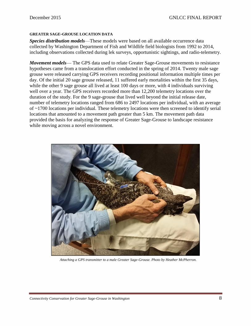
Movement models— The GPS data used to relate Greater Sage-Grouse movements to resistance

hypotheses came from a translocation effort conducted in the spring of 2014. Twenty male sage

grouse were released carrying GPS receivers recording positional information multiple times per

day. Of the initial 20 sage grouse released, 11 suffered early mortalities within the first 35 days,

while the other 9 sage grouse all lived at least 100 days or more, with 4 individuals surviving

well over a year. The GPS receivers recorded more than 12,200 telemetry locations over the

duration of the study. For the 9 sage-grouse that lived well beyond the initial release date,

number of telemetry locations ranged from 686 to 2497 locations per individual, with an average

of ~1700 locations per individual. These telemetry locations were then screened to identify serial

locations that amounted to a movement path greater than 5 km. The movement path data

provided the basis for analyzing the response of Greater Sage-Grouse to landscape resistance

while moving across a novel environment.

Attaching a GPS transmitter to a male Greater Sage-Grouse. Photo by Heather McPherron.



Objective 1: Species Distribution Modeling

Introduction

The WHCWG Columbia Plateau Analysis (WHCWG 2012) of sage grouse habitat connectivity

in Washington was based on coarse delineations of Habitat Concentration Areas (HCAs) where

sage grouse were known to be present. Ideally, HCA boundaries would be drawn from an

empirical species distribution model (SDM; Elith & Leathwick 2009) that spatially quantifies

areas on the landscape suitable for Greater Sage-Grouse. In addition to providing a more

rigorous delineation of the true extent of core areas, species distribution modeling can potentially

identify new areas that are suitable but currently unoccupied. Such areas might be targets for

establishing new subpopulations through natural colonization if they are accessible to occupied

habitat, or by translocations if they are too isolated. In addition, species distribution models may

also reveal important landscape variables and thresholds that are related to habitat occupancy.

In this study, we used species distribution modeling to identify factors associated with the

presence of sage grouse in the Columbia Basin of Washington State. We were also interested in

seasonal differences in sage grouse responses to environmental variables, as well as the spatial

scale at which these variables were important predictors of occurrence. Specifically, we sought

to (1) delineate suitable habitat areas throughout the Columbia Basin of Washington for each

biological season (breeding, nesting, brood-rearing, and winter), (2) update the WHCWG

Columbia Plateau Analysis Habitat Concentration Areas (HCAs) based on the mean habitat

suitability value across all seasons, (3) update the WHCWG Columbia Plateau Analysis barrier,

pinch point, and centrality models based on the new definition of HCAs, and (4) compare the

updated models to the original WHCWG Columbia Plateau Analysis to determine the extent of

change and the conservation implications.

Methods

The methods used to produce the species distribution models for sage grouse are described in the

attached manuscript titled Persistence of Greater Sage-Grouse (Centrocercus urophasianus) in

an Agricultural Landscape.

To produce new HCAs from the seasonal Greater Sage-Grouse habitat models, we first averaged

all four seasonal models (breeding, nesting, brood-rearing, and winter). We then used this mean

year-round probability of occurrence as an input for the GIS algorithm used to delineate HCAs,

as described in WHCWG (2012). Specifically, we used a 500 m moving window radius, required

an average habitat value of at least 0.2 within the window and per pixel, expanded the cores by

1000 m to connect nearby patches, and required a minimum core area size of 1000 ha.

We then used these empirically derived HCAs as the cores for assessing connectivity. We used

the Linkage Mapper toolkit to map linkages, barriers, pinch-points, and calculate centrality

scores for HCAs and linkages, as described in WHCWG (2012, 2013).

Results

The results from the species distribution modeling are described in the attached manuscript.

Updating sage grouse HCAs with the empirical distribution model resulted in a total of 10 HCAs

(Fig. 1, Figs. 3–6), compared to 4 HCAs defined in the WHCWG Columbia Plateau Analysis



(2012). The 4 largest HCAs (numbered 1, 2, 5, and 6 in Figs. 3–6 respectively) roughly

corresponded to the WHCWG (2012) HCA locations and the 4 subpopulations in the state

(Moses Coulee, Crab Creek, Yakima Training Center, and Yakama Nation). The 6 new HCAs

(mean area = 8159 ha) were much smaller than the 4 largest HCAs (mean area = 93,485 ha),

raising the issue of whether they were large enough to support a breeding population. Regardless,

their distribution between the larger cores makes them potential stepping stones that could serve

as stopovers for long-distance dispersers moving between the large HCAs.

Linkages connecting these HCAs followed a similar pattern to the WHCWG (2012) HCA

models, connecting each of the 4 largest HCAs and running through the smaller stepping stones

described above (Fig. 3). The presence of the stepping stones reduces the cost-weighted distance

between the 4 largest HCAs, underscoring their value as stopovers for Greater Sage-Grouse

dispersing between subpopulations.

The major barriers which added significant cost-distance to the linkages over small areas

corresponded to major transmission lines (Fig. 4). Transmission lines in this analysis and our

prior analysis of resistance (Shirk et al. 2015) appear to be major determinants of habitat

suitability and movement within the study area.

Within the linkages, major pinch-points appeared in several places where high resistance

funneled movement paths into narrow constrictions (Fig. 5). The most significant bottlenecks

appeared south of HCAs 1 and 3 (Moses Coulee) in a gap between a major transmission line and

a region of intensive agriculture, west of HCA 5 (Yakima Training Center) where the linkage

crosses highway 410, and east of HCA 6 (Yakama Nation) where the linkage passes through

intensive agricultural areas and across Interstate Highway 82.

The most central linkages and HCAs in the network, based on circuit theory current flow, were

comprised of the Yakima Training Center (HCA 5) and Colockum (HCA 7 and 8) HCAs and the

linkage between them (Fig. 6). Any loss of HCAs or linkages in this region would fragment the

population into two disconnected regions.

Discussion

There were several key findings from this analysis that can be used to guide conservation of

habitat and connectivity for Greater Sage-Grouse in the Columbia Basin. The attached

manuscript describes several habitat requirements that are strongly associated with sage grouse

occupancy, including a minimum of about 30% of the landscape comprised of native shrubsteppe

within a 5 km moving window, at least 2 km from the nearest transmission line, and a

configuration of habitat (both native shrubsteppe and CRP) characterized by large cores rather

than small isolated patches. Additionally, we found that when CRP was about 25% of more of

the landscape within a 5 km moving window, it significantly increased the suitability of areas

where native shrubsteppe was less extensive and more fragmented. At least some native

shrubsteppe was required in the local landscape for this benefit, however (i.e., CRP was not a

substitute for native habitat). The importance of the CRP program in augmenting habitat was

demonstrated by the ‘No CRP’ alternative scenario, which revealed a loss of 66% of suitable

habitat when CRP lands in our species distribution models were converted to wheat fields (see

attached manuscript). These relationships between landscape attributes and occupancy (including



the shape of the relationship as well as the scale of selection) provide a means to better manage

the landscape to best support a viable population of sage grouse.

Another benefit of the species distribution models we have produced is a more rigorous

delineation of areas that support sage grouse habitat requirements over the seasons of breeding,

nesting, brood-rearing, and winter. Not only does this provide a more spatially accurate

representation of HCAs associated with the four known breeding subpopulations, but it also

identified several smaller HCAs that could serve as stepping stones between the largest cores.

This revised set of HCAs (including the stepping stones) provides a slightly different network for

modeling connectivity, and this led to modest changes in the linkages, pinch-points, barriers, and

centrality models compared to the Columbia Plateau analysis (WHCWG 2012, 2013).

The biggest implication of this new network of habitat is presence of the stepping stone HCAs,

which reduce cost-distances between the larger occupied HCAs. If these stepping stones do, in

fact, serve as seasonal stopovers for long-distance dispersal events, they may serve a key role in

connecting the larger network, and these areas may warrant additional survey effort and

protections. Moreover, it is possible some of the larger stepping stones may even support a

breeding population.

Even when including stepping stones southeast of the YTC HCA, our revised linkage models

still predict very large cost-weighted distances (well over 100 km) between the YTC and the

newly introduced Yakama Nation population to the south. These large distances suggest the

Yakama Nation population is isolated from the rest of the network, perhaps explaining why

modeled habitat there was not naturally recolonized (the population was instead introduced via

translocation).

The current network of habitat and linkages is threatened by potential future changes in climate

and climate-related disturbance regimes. A recent analysis of five climatic niche models (i.e.,

spatial models that correlate species distributions with climate variables and make future

projections given climate change scenarios) predicts a contraction of between 37% and 79% of

the current sagebrush steppe biome in the Columbia Basin by the end of the century, and these

models generally agree that contraction is most likely to occur in the southwest portion of the

basin (Michalak et al. 2014). This region encompasses the Yakama Nation and the Yakima

Training Center HCAs (numbered 5, 6, 9, and 10 in Figs. 3–6). Contraction of the sagebrush

biome to exclude the YTC would be a major loss, as it represents about a third of the population

and the largest block of native shrubsteppe habitat in the state. However, the above study

projected expansion of sagebrush steppe by between 63% and 165% of the current area

(depending on the climate change scenario), mainly in the northern portion of the basin

(Michalak et al. 2014). If the current population was connected to expanding habitat in the north,

it may provide a means to offset the loss of habitat where the YTC population resides and allow

the population to shift its range and track its climate envelope.

The Lund-Potsdam-Jena Dynamic Global Vegetation Model, a mechanistic model based on

biological processes, population dynamics, and species competition, projects a very different

future Columbia Basin biome distribution by the end of the century. Under this approach, 4 of

the 5 climate models described above agree that most of the sagebrush steppe biome will



transition to grasslands and open forests (Michalak et al. 2014). Indeed, encroachment of forests

into sagebrush habitats has already been observed (Hyerdahl et al. 2006). If the future Columbia

Basin matches the mechanistic model projections, the current network of HCAs and linkage

would be unsuitable for sage grouse. Monitoring of forest encroachment appears warranted and

adaptation responses may include suppression of forests to maintain shrubsteppe.

The frequency and intensity of wildfire in the future will likely be a major influence on the

sagebrush biome. Historically fire suppression and reduction in fuels due to grazing and

conversion to agriculture has resulted in low fire frequency and intensities. Sagebrush can

recolonize burned areas if the intensity is sufficiently low that some plants survive and can re-

seed, and if seedlings have time to establish. The frequency and intensity of fires is projected to

increase in the region, although climate models differ in the magnitude and timing of these

changes (Rogers et al. 2011). If the future fire regime exceeds the intensity and frequence

thresholds for survival and establishment of sagebrush species, fire could be a major factor

driving transition of sagebrush to grasslands, as predicted by the mechanistic model described

above.

Clearly there is great uncertainty about the future distribution of sagebrush steppe in the

Columbia Basin landscape. However, regardless of how the future unfolds, habitat connectivity

to existing and future habitat areas will almost certainly be critical to maintaining a viable

population of Greater Sage-Grouse in this landscape. Habitat connectivity will allow the

population to track its shifting habitat and maintain robust demographic and genetic exchange

that is key to functional metapopulations. This analysis demonstrates the degree to which human

modification of the landscape, particularly agriculture and transmission lines, has fragmented the

population and limited connectivity among the major remaining remnant patches. Our

observation that CRP lands are valuable in augmenting habitat suitability (see attached

manuscript) and offer low resistance to movement (Shirk et al. 2015) suggests a means by which

the area of habitat and connectivity may be increased through reallocation of CRP enrollments.

The allocation of CRP in this landscape could be shifted over time to reflect the changing

distribution of the sagebrush steppe biome, and thereby provide an adaptive management tool for

sage grouse conservation in a changing climate and landscape.



Figure 3. Linkages connecting HCAs followed a similar pattern to the WHCWG (2012) HCA

models connecting each of the 4 largest HCAs (numbered 1, 2, 5, and 6) and running through the

smaller stepping stones (HCAs 3, 4, 7, 8, 9, and 10).



Figure 4. Barriers which added cost-weighted distance to linkages for Greater Sage-Grouse.

Areas of highest barrier strength correspond to locations of major transmission lines.



Figure 5. Linkage pinch-points for movement of Greater Sage-Grouse.



Figure 6. Linkage network centrality for Greater Sage-Grouse.



Objective 2: Movement Modeling

Introduction

The translocation effort conducted by WDFW provided a unique opportunity to analyze GPS

telemetry data from radio-marked Greater Sage-Grouse in conjunction with existing and ongoing

research. As well, the release offered a chance to evaluate existing models of landscape

resistance based on previous studies of sage grouse landscape connectivity (Shirk et al 2015).

Essentially, the analysis of GPS location data for translocated Greater Sage-Grouse was a test of

alternative hypotheses developed to explain and understand how sage grouse respond to

landscape features. We theorized that after release sage grouse would move around or explore

the landscape for periods of time before eventually settling or establishing a localized home

range. These exploratory moves were the basis for evaluating the different resistance surfaces

and landscape connectivity.

Methods

Characterization and estimation of the exploratory movements was done with the use of the

Brownian bridge movement model of space use (Horne et al. 2008). The Brownian bridge

movement model (BBMM) offers a convenient and spatially explicit estimation of probabilities

of space use between known telemetry locations. Initially, the telemetry data were screened to

identify consecutive locations that exceed 5 km in length, thereby representing an exploratory

movement path. A minimum of 3 locations were used per path, with up to 10 telemetry locations

per path in total. Once each path was identified the probability of use along the path was

estimated with the BBMM package in program R (R Core Team 2015). Each individual path was

then combined and evaluated against each hypothesis as characterized by landscape resistance

surfaces.

Each of the hypotheses described by landscape connectivity was represented as a 30-m GIS

raster layer representative of the resistance surface (Fig. 7). These resistance surfaces are

previously described by Shirk et al. (2015). For this portion of the study we focused on the 30

fine-scale models in Supplement 2 of Shirk et al. (2015), including a null model, where

landscape resistance for the entire landscape was set to 1. Prior to combination with the BBMM,

for each of the 30 resistance surfaces, and for each individual path, least-cost corridors (LCC)

were generated from accumulated cost surfaces. Accumulated costs surfaces were derived from a

transitional layer, or graph, based upon the original resistance surface using the raster (Hijaman

and van Etten 2012) and gdistance (van Etten 2015) packages in R. Each resistance surface was

initially cropped to the extent of each of the BBMM paths. This greatly reduced processing time

and allowed for the summation of weighted costs for each BBMM from the first telemetry

location in the path to the last. Each LCC was also normalized, with the least-cost path equal to

zero, so comparisons among paths and hypotheses could be done, as well as population

averaging. Each BBMM, for each path, was multiplied by the corresponding LCC generating a

weighted LCC based on the BBMM probabilities. These weighted probability values were

averaged and divided by the average BBMM probability of each path to give an average

probability weighted LCC value for each path. Subsequent compilation and analysis of results

were based on these weighted probability values of average LCC across the BBMM distribution

for each path.



With the spatial analysis complete, further statistical analysis was required to establish any

patterns in the results and for further inference to landscape and anthropogenic features.

Therefore, to compare the average, probability weighted LCC values of each path and

hypothesis, we ranked the averaged values combined over all paths and used non-parametric

statistics to test for differences among hypotheses. We also tested for differences between those

sage grouse that lived well beyond the release and those which died shortly after release. We

used the Kruskal-Wallis test to test for difference between early mortalities and survivors, and

for overall difference of hypotheses. Multiple comparisons after the Kruskal-Wallis test were

done in R with the kruskalmc command from package pgirmess in R (2015 R Core Development

Team) based on the Siegel and Castellan (1988). Once differences among hypotheses were

defined and understood, the hypotheses could be interpreted in relation to the GPS telemetry data

and further spatial dynamics related to sage grouse landscape connectivity could be explored.

Initially, we expected to update existing models of spatial dynamics including linkage, pinch-

point, barrier and centrality models to reflect testing of the GPS data and resistance surfaces.

This however, proved not to be warranted as discussed below.

Updating the linkage, pinch-point, barrier and centrality models for sage grouse in those

historical areas where current conservation is ongoing can be done relatively quickly and is

straightforward (McRae et al. 2008, WHCWG 2013). The software and programs used for

creating these layers is available from circuitscape.org and requires the additional data input of

core habitat areas, provided by WHCWG (2013). The resistance surfaces used were those of the

Shirk et al. (2015) and selected based upon the average weighted least-cost corridor values.

Circuitscape also offers a program to create new resistance surfaces. However, as will be

discussed, we did not find merit in updating existing linkage models based on our findings.

Results

Comparison of results between sage grouse that suffered early mortality and sage grouse that

survived for more than 100 days, showed no difference overall in probability weighted LLC.

(Kruskal-Wallis X2 = 2.08; p = 0.15). Sage grouse that died shortly after release did not have a

different response to the resistance layers, in general, than those that survived well beyond

release. Although, the smaller sample size of BBMM paths for early mortalities (n = 59) than

those of survivors BBMM paths (n = 317) could well play a part in this finding. Since the overall

goal was to discern how sage grouse responded to the landscape, understanding if the resistance

surfaces could characterize the difference in survivorship was a relevant analysis. Had there been

a statistically significant difference in probability weighted LLC between early mortalities and

survivors some further analysis and conclusion may have been inferred. However, the fact that

no differences were found is in itself an informative finding for gleaning down future decision

making. It appears that the use of the landscape, as portrayed by the combination of sage grouse

movement paths and landscape resistance surfaces in this study, did not differ between early

mortalities and long surviving sage grouse.

The averaged probability weighted LLCs for each path and hypothesis were tallied and ranked

(Table 1). These values represent the average probability weighted LLC value of each cell, or

pixel, for each resistance surface, or hypothesis. Or in other words, the LLC for each pixel after

being weighted by the probability of use as defined by the BBMM. The tally and ranking of the

resistance surfaces for the early mortalities (Table 1) are similar to those of the survivors. The



first 3 resistance surfaces and the last 4 were identical between early mortalities and long-

surviving sage grouse. Slight differences in rank position are shown by the double-sided arrows

in Table 1 and show only minor discrepancies. The greatest difference in rank is only six places

for resistance surface 54. The resistance surface number directly correlates with the models

shown in the tables of Shirk et al. (2015).

Further analysis based on non-parametric statistics showed there was a difference in probability

weighted LLC among the resistance layers for those sage grouse surviving more than 100 days

(Kruskal-Wallis X2 = 136.22; p = >7.9e -16). Contrary, there was no difference in probability

weighted LLC (Kruskal-Wallis X2 = 31.86; p = 0.326) for those that died early on, shown in red

in Table 1. Therefore, no further multiple comparisons were conducted for the early mortalities,

but were conducted on the longer surviving sage grouse. Multiple comparisons of the long-

surviving sage grouse showed three distinct groupings of different weighted probability LLCs

among the resistance surfaces. The highlighted text in Table 1, illustrate which models showed

differences. Essentially the first 4 resistance surfaces highlighted in yellow were all significantly

different than the last 5 resistance surfaces shown in yellow. None of these however, showed any

significant difference with those models ranked between the 2 groupings, lacking any

highlighting. Nor were there any differences within the first 4, nor within the last 5 resistance

surfaces. The null model, # 52, showed significant differences with all those ranked 18th place,

and are shown in boldface. Examples of the Greater Sage-Grouse GPS telemetry data with

contoured or rasterized BBMM paths overlaid on an example resistance surface are shown in

Figures 7–11 below. These examples are all of sage grouse that survived well beyond the initial

release.

Male Greater Sage-Grouse wearing GPS transmitter. Photo by Michael A. Schroeder.



Discussion

The highest ranked resistance surfaces correspond to models representing differing features on

the landscape. In this case, the null model had the lowest overall average LLC values. This was

the case for both long-surviving Greater Sage-Grouse and sage grouse that suffered early

mortality. In general, there did not appear to be much difference in the overall ranking of early

mortality sage grouse and long-surviving sage grouse. We did not find evidence that perception

of the landscape, as represented by the alternative resistance models, was different between

early-mortalities and long-surviving sage grouse. Nor was a significant difference among the

early-mortality results based on the Kruskal-Wallis test. This may be due to the much smaller

sample size and the actual nature of the mortalities, i.e., via predation, translocation-stress, GPS

unit complications, etc. The limited data on the early mortalities appeared no different than

surviving sage grouse in this analysis.

Beyond the null model, the lowest average LLC values for long surviving sage grouse

corresponded to models 74, 55, 76 & 79. Notably these 5 models (null included) all differed

significantly from the highest average values found at the bottom of Table 1. Finding the null

model as the lowest resistance surface offers an important context for interpretation of the

results. There are a variety of possible explanations and implications that can be inferred from

this finding, however there are additional avenues of research that need to be done to verify and

either collate or to question these findings. Keeping the finding of the null model in relation to

the other 29 resistance surfaces is important, as is understanding the findings of the 29 resistance

models without considering the null. As will be discussed below, the magnitude of the initial

resistance values may bias the results in favor of the null.

A closer look at the next four highest ranked models showed some similarities in their patterns of

resistance. The highest ranked resistance surface, # 74 was developed based on expert opinion

and also included elevation as a main resistance factor. The second highest ranked model, # 55

included pasture converted to Conservation Reserve Program land (CRP) as the major resistance

factor, with minor resistance due to major highways, secondary highways, railways, transmission

lines, and wind turbines. The third highest ranked resistance surface, # 76, represents the

combination of the highest ranked, # 74, and the second highest ranked, # 76. The fourth highest

resistance model, # 79, was similar to the highest rank model, # 76, except for the resistance

values of the transmission lines were doubled. The null model however, represents a landscape

where the resistance was initially set to 1 and the least-cost corridor. Actual resistance values

from the 4 top ranked resistance surfaces ranged from 0 to 99.

The multiple comparison of means suggested however that these models really were not any

different than the null model. This could be due to a variety of reasons. Given the initial broad

extent of the resistance surfaces (Fig. 1), and the greatly reduced extent of individual BBMMs,

each of the resistance surfaces that did not differ from the null, may have actually been

approximating the null model. If, due to the limited extent of the BBMM, there were only

original values of 1 in the alternative resistance surface, then each alternative is really on average

no different than the null. In other words, there could be a lack of heterogeneity in the resistance

surfaces and accumulated cost surfaces at the fine scale that the BBMM estimates within.



Looking deeper however, we find that the null model suggests that the lowest resistance and

consequently the least-cost path is found in straight line from the first GPS telemetry point to the

last GPS telemetry point of each 5 km path. Now in theory, were the middle GPS points(s), and

the corresponding BBMM, not along or that straight, and for example in a large C-shaped curve,

then an alternative resistance model that truly was the “correct” model would have a least-cost

path that follows the C-shaped curve, and consequently, a lower overall average LCC. The

minimum values along the least-cost path are zero. Deviations away from the LCC, as reflected

in the accumulated cost surface, result in an increase in LCC values. In particular, if the straight

line between the first and last point crossed through a particularly resistant surface, for example,

a small mountain range, a town, or even a large body of water the accumulated cost values for

that straight line, could in theory become quite large for the null hypothesis. How large those

accumulated cost values becomes depends on how far spatially the deviation to the null straight

line path is from the alternative LCC, and also the resistance values themselves. In this study,

resistance values range from 0 to 99, while the null was set to 1. If these values are not

commensurate with the null and how sage grouse actually travel through space and time then the

very magnitude of the resistance values may in fact be too large to detect a deviation from the

straight line path, or the null model. Basically, as deviations from the LCP are created in an

accumulated cost surface, the values may become so large that only C-shaped curves which are

heavily exaggerated could possibly have lower average LCP values. In particular, exaggerated C-

shaped moves by sage grouse may occur relatively quickly in time, thereby narrowing the

BBMM probability distribution. Movement paths of 5 km that were relatively straight have less

of an opportunity to have a lower average LCP than the null model due to the magnitude of

resistance values, thus possibly biasing the findings in favor of the null.

The evidence supporting the null model as the resistance surface with the lowest average

weighted LLC may in fact be biased based upon the very resistance values themselves. Or

possibly the extent of the BBMM has actually reduced the heterogeneity of the resistance

surfaces to such a point that the resistance surfaces are approximating the null resistance model.

In either case, further refinement in the modeling process to assess the potential for bias and for

developing fine-scale resistance models that have sufficient heterogeneity at the extent of the

sage grouse BBMM needs to be done. Likewise given the likely changes in behavior as a sage

grouse moves along a 5 km path, additional consideration should be given to including the

results of the habitat analysis into the resistance models. Therefore, future investigation of these

GPS data and resistance models needs to be completed prior to updating linkage, pinch-point,

barrier, and centrality models based on circuitscape theory (McRae et al.2008). Proceeding to the

intended analysis and revaluation of linkage, pinch-points, barriers, and centrality models were

not warranted based upon the findings of the null model being lowest ranked. Preliminary

linkage models were developed based on the average values of the top 4 resistance surfaces, but

were not presented here to do the shortcomings of our findings. Existing linkage, pinch-point,

barrier and centrality model were nearly identical to those preliminary models developed.

None the less, this data analysis has provided a streamlined methodology for evaluating

probabilities of space use by GPS collared Greater Sage-Grouse with resistance models and

circuit theory of animal movement. This demonstration has provided insight into the modeling

process and a possible bias for further development and research into patterns of sage grouse

movement. The preliminary results also suggest, at least out of the ranked ordering, which



resistance models should be included in further evaluation and possible factors impacting sage

grouse as they explored this novel landscape.

Future Direction

The particular refinements to our approach that need to be done include exploring the bias

towards the null due to magnitude of resistance values and bringing the results of the habitat

model into the resistance surface creation. Adjusting the magnitude of resistance values can be

done systematically to see if and when there is any evidence of a resistance surface having a

lower LLC than the null. If there is a point at which this takes place, some simulated data and

analysis may be helpful in determine the extent of deviations that need to occur spatially, prior to

having an expectation for accumulated cost distances to tend lower for alternative resistance

surfaces. Exploration of resistance magnitude and the overall shape of movements paths, i.e.,

straight or curved, should be done to follow up and advance the findings presented here.

Simulation analysis can provide a relatively quick way to understand these potential biases.

Additionally, given the linear nature of roads and transmission lines across the landscape, it is

reasonable to assume that as a sage grouse travels across the landscape, the easiest and best way

to cross the linear feature is directly and quickly. In this case, the high resistance values of those

features, may not be reflected by the accumulated, weighted LCC values, and essentially missed.

The large contiguous portions of the resistance surface and accumulated cost surface my override

any signal that could be expected form a linear feature. Especially if the crossing took place

quickly, as the greater the distance traveled per unit of time tends to narrow a BBMM thereby

lowering the accumulated cost of the liner feature. Therefore, attempting to understand how sage

grouse respond to these linear features might more appropriately be addressed following the

example of Horne et al. (2007). Future analysis of these data could follow up with a general

linear modeling of BBMM in response to covariates describing known crossings of roads,

transmission lines, and any other liner feature of interest. This may provide a more direct

assessment of the influence of linear features like roads and transmission lines on space-use by

sage grouse then the evaluation of landscape resistance model, where the influence of the linear

features are essentially nested in the resistance model and not specifically addressed.



Table 1. Ranking of landscape resistance surfaces based on the weighting of least-cost corridors (LCC) by the Brownian bridge movement model (BBMM) probabilities showing the average LCC values of each resistance surface, the differences in ranks between Greater Sage-Grouse suffering early mortality vs. long-surviving sage grouse (arrows), and the groupings based on multiple comparison of means (yellow highlight).

Rank

Resistance

surface

Long-

surviving

Resistance

surface

Early

mortalities

NULL 52 67.3112 52 61.2073

1 74 70.0215

74 61.9035

2 55 75.6457

55 71.1334

3 76 78.6056

76 72.1578

4 79 78.8219

60 73.5116

5 60 80.8701

77 74.2688

6 78 81.8346

79 78.8085

7 77 83.9195

58 79.0326

8 71 85.0327

78 79.9790

9 57 85.4671

57 81.7647

10 58 87.5237

71 82.9909

11 56 89.9008

56 84.2900

12 53 91.0386

72 85.0257

13 59 91.0386

53 85.9124

14 67 91.0386

59 85.9124

15 64 92.0174

67 85.9124

16 72 92.5659

64 86.5626

17 73 94.3585

73 86.9517

18 66 94.6480

65 90.2494

19 65 96.5712

61 90.5123

20 61 97.2027

54 92.4628

21 80 98.0375

66 93.8775

22 68 101.3546

80 95.0265

23 62 102.5289

62 97.2812

24 63 103.8187

68 98.9202

25 54 104.2356

63 99.3746

26 81 104.8488

81 100.1432

27 69 113.9205

69 111.0471

28 70 115.2346

70 113.4254

29 75 118.8686

75 114.6158



Figure 7. Example map showing Greater Sage-Grouse GPS telemetry data with contoured or rasterized

BBMM paths overlaid on an example resistance surface (sage grouse ID # 13720). Darker areas of the

background landscape indicate higher resistance values, while the red lines indicated state highways and

roads.




BBMM paths overlaid on an example resistance surface (sage grouse ID # 13721; some telemetry data

removed). Darker areas of the background landscape indicate higher resistance values, while the red lines

indicated state highways and roads.






roads.



Literature Cited

Aldridge, C. L. 2005. Identifying habitats for persistence of Greater Sage-Grouse (Centrocercus

urophasianus). PhD dissertation. University of Alberta, Edmonton, Alberta.

Aldridge, C. L., and M. S. Boyce. 2007. Linking occurrence and fitness to persistence: habitat

based approach for endangered Greater Sage-Grouse. Ecological Applications 17:508–

526.

Aldridge, C. L., and R. M. Brigham. 2003. Distribution, abundance, and status of the Greater

Sage-Grouse, Centrocercus urophasianus, in Canada. Canadian Field Naturalist 117:25–

34.

Aldridge, C. L., S. E. Nielsen, H. L. Beyer, M. S. Boyce, J. W. Connelly, S. T. Knick, and M. A.

Schroeder. 2008. Range-wide patterns of Greater Sage-Grouse persistence. Diversity and

Distributions 14:983–994.

Benedict, N. G., S. J. Oyler-McCance, S. E. Taylor, C. E. Braun, and T. Quinn. 2003. Evaluation

of the Eastern (Centrocercus urophasianus urophasianus) and Western (Centrocercus

urophasianus phaios) subspecies of Sage-grouse using mitochondrial and control-region

sequence data. Conservation Genetics 4:301–310.

Braun, C. E. 1986. Changes in Sage Grouse lek counts with advent of surface coal mining.

Proceedings of Issues and Techniques in the Management of Impacted Western Wildlife

2:227–231.

Cadwell, L. L., M. A. Simmons, J. J. Nugent, and V. I. Cullinan. 1997. Sage-grouse habitat on

the Yakima Training Center: Part II, Habitat Modeling. PNNL-11758. Pacific Northwest

National Laboratory, Richland, Washington.

Campbell, R. W., N. K. Dawe, I. M. Cowan, J. M. Cooper, G. W. Kaiser, and M. C. E. McNall.

1990. The birds of British Columbia. Vol. 2. Royal British Columbia Museum, Victoria.

Connelly, J. W., M. A. Schroeder, A. R. Sands, and C. E. Braun. 2000. Guidelines to manage

sage grouse populations and their habitats. Wildlife Society Bulletin 28:967–985.

Connelly, J. W., S. T. Knick, M. A. Schroeder, and S. J. Stiver. 2004. Conservation assessment

of Greater Sage-Grouse and sagebrush habitats. Unpublished report. Western Association

of Fish and Wildlife Agencies, Cheyenne, Wyoming.

Hanser, S. E., and S. T. Knick. 2011. Greater Sage-Grouse as an umbrella species for shrubland

passerine birds. Pages 475–488 in S. T. Knick and J. W. Connelly editors. Greater Sage-

Grouse: ecology and conservation of a landscape species and its habitats. Studies in

Avian Biology Series (vol. 38), University of California Press, Berkeley, California. In

press.



Hays, D. W., M. J. Tirhi, and D. W. Stinson. 1998. Washington State Status Report for the Sage

Grouse. Washington Department of Fish and Wildlife, Olympia.

Hijmans, R. J., and van Etten, J. 2012. raster: Geographic data anlaysis and modeling. R package

version 2.0-31, Available from http://CRAN.R-project.org/package=raster.

Holloran, M. J., R. C. Kaiser, and W. A. Hubert. 2010. Yearling Greater Sage-Grouse response

to energy development in Wyoming. Journal of Wildlife Management 74:65–72.

Horne, J. S., E. O. Garton, S. M. Krone, and J. S. Lewis. 2007. Analyzing animal movements

using Brownian Bridges. Ecology 88:2354–2363.

Heyerdahl, E. K., R. F. Miller, and R. A. Parsons. 2006. History of fire and Douglas-fir

establishment in a savanna and sagebrush–grassland mosaic, southwestern Montana,

USA. Forest Ecological Management 230:107–118.

Johnson, D. H., M. J. Halloran, J. W. Connelly, S. E. Hanser, C. L. Amundson, and S. T. Knick.

2011. Influences of environmental and anthropogenic features on Greater Sage-Grouse

populations, 1997–2007. Pages 407–450 in S. T. Knick and J. W. Connelly, editors.

Greater Sage-Grouse: ecology and conservation of a landscape species and its habitats.

Studies in Avian Biology Series (vol. 38), University of California Press, Berkeley,

California.

Knick, S. T., and S. E. Hanser. 2011. Connecting pattern and process in greater sage-grouse

populations and sagebrush landscapes. Pages 383–406 in S. T. Knick and J. W. Connelly

editors. Greater Sage-Grouse: ecology and conservation of a landscape species and its

habitats. Studies in Avian Biology Series (vol. 38), University of California Press,

Berkeley, California.

Knick, S. T., S. E. Hanser, and K. L. Preston. 2013. Modeling ecological minimum requirements

for distribution of greater sage-grouse leks: implications for population connectivity

across their western range, U.S.A. Ecology and Evolution (Open Access) 1–13.

Livingston, M. A. 1998. Western Sage grouse management plan. Department of the Army,

Directorate of Environmental and Natural Resources, Yakima Training Center, Yakima,

Washington.

Lyon, A. G., and S. H. Anderson. 2003. Potential gas development impacts on sage grouse nest

initiation and movement. Wildlife Society Bulletin 31:486–491.

MaRae, B. H., B. G. Dickson, T. H. Keitt, and V. B. Shah. 2008. Using circuit theory to model

connectivity in ecology and conservation. Ecology 10:2712–2724.

McClintock, B. T., D. S. Johnson, M. B. Hooten, J. M. Ver Hoef, and J. M. Morales. 2014.

When to be discrete: the importance of time formulation in understanding animal

movement. Movement Ecology 2:21.

http://cran.r-project.org/package=raster



Michalak, J. L., J. C. Withey, J. J. Lawler, S. Hall, and T. Nogeire. 2014. Climate vulnerability

and adaptation in the Columbia Plateau, Washington. School of Environmental and

Forest Sciences. University of Washington, Seattle, WA.

Oyler-McCance, S. J., and T. W. Quinn. 2011. Molecular insights into the biology of Greater

Sage-Grouse. Pages 85–94 in S. T. Knick and J. W. Connelly editors. Greater Sage-

Grouse: ecology and conservation of a landscape species and its habitats. Studies in

Avian Biology Series (vol. 38), University of California Press, Berkeley, California.

Oyler-McCance, S. J., S. E. Taylor, and T. W. Quinn. 2005. A multilocus population genetic

survey of the Greater Sage-Grouse across their range. Molecular Ecology 14:1293–1310.

R Core Team. 2015. R: A language and environment for statistical computing. R Foundation for

Statistical Computing, Vienna, Austria. Available from https://www.R-project.org/.

Rogers, B. M., R. P. Neilson, R. Drapek, J. M. Lenihan, J. R. Wells, D. Bachelet, and B. E. Law.

2011. Impacts of climate change on fire regimes and carbon stocks of the US Pacific

Northwest. Journal of Geophysical Resources. Biogeosciences 116:2005–2012.

Schroeder, M. A., J. R. Young, and C. E. Braun. 1999. Sage grouse (Centrocercus

urophasianus). Pages 1–28 in A. Poole and F. Gill, editors. The Birds of North America

No. 425. The birds of North America, Philadelphia, Pennsylvania.

Schroeder, M. A., D. W. Hays, M. F. Livingston, L. E. Stream, J. E. Jacobson, and D. J. Pierce.

2000. Changes in the distribution and abundance of sage grouse in Washington.

Northwestern Naturalist 81:104–112.

Schroeder, M. A., and M. Vander Haegen. 2003. Migration Patterns of Greater Sage-Grouse in a

Fragmented Landscape. Progress Report. Washington Department of Fish and Wildlife,

Olympia, Washington.

Schroeder, M. A., and W. M. Vander Haegen. 2011. Response of greater sage-grouse to the

Conservation Reserve Program in Washington State. Pages 517–529 in S. T. Knick and J.

W. Connelly, editors. Greater Sage-Grouse: ecology and conservation of a landscape

species and its habitats. Studies in Avian Biology Series (vol. 38), University of

California Press, Berkeley, California.

Schroeder, M. A., D. Stinson, and M. Tirhi. 2003. Greater sage-grouse (Centrocersus

urophasianus). Priority Habitat and Species Management Recommendations Vol. IV:

Birds. 19pp.

Schroeder, M. A., C. L. Aldridge, A. D. Apa, J. R. Bohne, C. E. Braun, S. D. Bunnell, J. W.

Connelly, P. A. Deibert, S. C. Gardner, M. A. Hilliard, G. D. Kobriger, S. M. McAdam,

C. W. McCarthy, J. J. McCarthy, D. L. Mitchell, E. V. Rickerson, and S. J. Stiver. 2004.

Distribution of sage-grouse in North America. Condor 106:363–376.

https://www.r-project.org/



Schroeder, M. A., D. Stinson, H. Ferguson, M. Atamian, and M. Finch. 2008. Re-introduction of

sage-grouse to Lincoln County, Washington. Progress Report. Washington Department of

Fish and Wildlife, Olympia, Washington.

Schroeder, M. A., M. Atamian, H. Ferguson, M. Finch, K. Stonehouse, and D. Stinson. 2013.

Re-introduction of Greater Sage-Grouse to Lincoln County, Washington: Preogress

Report. Washington Department of Fish and Wildlife Final Report to the USFWS.

Shirk, A, J., M. A. Schroeder, L. A. Robb, and S. A. Cushman. 2015. Empirical validation of

landscape resistance models: insights from the Greater Sage-Grouse (Centrocercus

urophasianus). Landscape Ecology 30:1837–1850.

Siegel, S., and N. J. Castellan. 1988. Nonparametric statistics for the behavioral sciences.

MacGraw Hill Int., New York.

Stinson, D. W., D. W. Hays, and M. A. Schroeder. 2004. Washington State recovery plan for the

greater sage-grouse. Washington Department of Fish and Wildlife, Olympia,

Washington.

USDA (United States Department of Agriculture). 2015. CRP enrollment and rental payments by

County and State, 1986-2014. http://www.fsa.usda.gov/programs-and-

services/conservation-programs/reports-and-statistics/conservation-reserve-program-

statistics.

Van Etten, J. 2015. gdistance: Distance and routes on geographical grids. R package version 1.1-

9, Available from http://CRAN.R-project.org/package=gdistance.

WHCWG (Washington Wildlife Habitat Connectivity Working Group). 2012. Washington

Connected Landscapes Project: Analysis of the Columbia Plateau Ecoregion.

Washington’s Department of Fish and Wildlife, and Department of Transportation,

Olympia, WA. Available from http://www.waconnected.org

WHCWG (Washington Wildlife Habitat Connectivity Working Group). 2013. Columbia Plateau

Ecoregion Connectivity Analysis Addendum: Habitat Connectivity Centrality, Pinch-

Points, and Barriers/Restoration Analyses. Washington’s Department of Fish and

Wildlife, and Department of Transportation, Olympia, WA. Available from

http://www.waconnected.org

Wisdom, M. J., C. W. Meinke, S. T. Knick, and M. A. Schroeder. 2011. Factors associated with

extirpation of Sage-Grouse. Pages 451–472 in S. T. Knick and J. W. Connelly, editors.

Greater Sage-Grouse: ecology and conservation of a landscape Species and its habitats.

Studies in Avian Biology Series (vol. 38), University of California Press, Berkeley,

California.

http://cran.r-project.org/package=gdistance





Presentations

Shirk, A. J., M. A. Schroeder, and L. A. Robb. 2015. A new empirical habitat model for sage-

grouse in the columbia basin: implications for the conservation reserve program. Washington

Sage Grouse Working Group. October 28th, 2015, Moses Lake, WA.

Habitat Occupancy and Movements by Greater Sage-Grouse …...Aldridge & Brigham 2003; Schroeder et...

Documents

Transcript of Habitat Occupancy and Movements by Greater Sage-Grouse …...Aldridge & Brigham 2003; Schroeder et...