
TEL.: (+264-61) 257411 FAX.: (+264) 88626368 CELL.: (+264 ...

8/14/2019 H.264 Compressed Shot Detection
http://slidepdf.com/reader/full/h264-compressed-shot-detection 1/128
COMPRESSED DOMAIN H.264/AVC SHOT DETECTION
Hugo Santos Varandas
Dissertação para obtenção do grau de Mestre em
Engenharia Electrotécnica e Computadores
Júri
Presidente: Prof. António Topa
Orientador: Prof. Fernando Pereira
Vogal: Prof. Paulo Correia
Outubro de 2008

8/14/2019 H.264 Compressed Shot Detection
http://slidepdf.com/reader/full/h264-compressed-shot-detection 2/128

8/14/2019 H.264 Compressed Shot Detection
http://slidepdf.com/reader/full/h264-compressed-shot-detection 3/128
Acknowledgments
First of all, I would like to thank my family, especially my father, mother and sister, for the provided
support and patience throughout all my academic career so far, particularly in the last semester.
I would also like express my gratitude to Prof. Fernando Pereira, who tutored this work, for his kind
suggestions and careful remarks. His support, patience and dedication certainly made this work easier
to develop.
I would also like to thank to all teachers of “Colégio do Sagrado Coração de Maria” and of “Instituto
Superior Técnico” who contributed to my academic formation.
Last, but not least, a big thank to all my friends and colleagues who have always been by my side
through all these years.
i

8/14/2019 H.264 Compressed Shot Detection
http://slidepdf.com/reader/full/h264-compressed-shot-detection 4/128
ii

8/14/2019 H.264 Compressed Shot Detection
http://slidepdf.com/reader/full/h264-compressed-shot-detection 5/128
Abstract
Nowadays, due to the advances in media coding and the increased availability of computer and
network resources, the usage of digital video is widespread to the general public. This gives rise to
new applications based on digital video, such as digital libraries and video-on-demand, which use
large collections of video. Moreover, the increasing importance of user generated content made digital
video more familiar to the general public leading to an exponential increase in video content creation.
This increase in video content availability originates the need of providing applications to efficiently
browse and consume large amounts of video data, like content-based video retrieval and
summarization applications. A fundamental step of these applications is to perform the temporal
segmentation of the video into its elementary units; the unit most commonly used in this context is the
shot, thus there is a growing need for shot transition detection applications. As digital video is usually
compressed, shot detection algorithms benefit from operating directly on the compressed bitstream
domain, without having to decompress the video and thus accept the associated decoding complexity.
The video coding standard emerging in a large range of application domains is the H.264/AVC
standard which provides a major compression efficiency improvement at the cost of a significant
increase in encoding and decoding complexity. The increased usage of compressed content further
increases the need for efficient compressed domain shot transition detection solutions.
The main objective of this Thesis is the design, implementation and evaluation of a shot transition
detection algorithm operating in the H.264/AVC compressed domain for both hard and gradual
transitions. In this report, the motivations, the state-of-the-art, the adopted architecture and the
implemented algorithms are presented. Finally, a detailed performance analysis is carried out
considering various alternative algorithms.
Keywords: Shot transition detection; H.264/AVC; Hard and Gradual Transitions; Hierarchical
Detection; Suspect GOP; Prediction Modes.
iii

8/14/2019 H.264 Compressed Shot Detection
http://slidepdf.com/reader/full/h264-compressed-shot-detection 6/128
iv

8/14/2019 H.264 Compressed Shot Detection
http://slidepdf.com/reader/full/h264-compressed-shot-detection 7/128
Resumo
Hoje em dia, devido aos desenvolvimentos recentes na codificação de multimédia e à disponibilidade
crescente de recursos computacionais e de rede, a utilização de vídeo digital tem-se disseminado,
estando presentemente disponível ao utilizador comum. Têm surgido novas aplicações que
necessitam de grandes quantidades de vídeo digital, como a televisão interactiva ou as videotecas.
Estas aplicações, associadas à popularidade crescente do vídeo gerado pelo utilizador (Youtube),
têm provocado um aumento exponencial na criação de vídeo digital. Por esse motivo, a necessidade
de aplicações de procura e sumarização de conteúdos multimédia, que providenciam uma forma mais
eficiente de utilizar este conteúdo, tem aumentado. Um processo fundamental em qualquer uma
destas aplicações é a divisão temporal do vídeo em unidades elementares, sendo o shot a unidade
elementar mais utilizada para esse efeito. Por isso, existe a necessidade de desenvolvimento de
aplicações de detecção de shot , ou, de transição entre shots.
Uma vez que o vídeo digital está, normalmente, na sua forma comprimida, os algoritmos de detecção
de shot beneficiariam em processar directamente no domínio comprimido, evitando a descompressão
do vídeo e poupando tempo no processo. A norma recente de codificação de vídeo H.264/AVC tem
sido largamente adoptada em diversas aplicações, devido à grande melhoria que proporciona na
compressão de vídeo. Como este aperfeiçoamento é acompanhado de um aumento significativo na
complexidade da codificação e descodificação, a necessidade de realizar a segmentação temporal de
vídeos directamente no domínio comprimido tem aumentado.
O objectivo principal desta dissertação é o projecto, implementação e avaliação de algoritmos que
efectuem a segmentação temporal de vídeos operando no domínio comprimido. Neste documento, as
motivações, o estado de arte, a arquitectura utilizada e os algoritmos implementados são descritos.
Uma análise ao desempenho dos vários algoritmos implementados é também apresentada.
Palavras-Chave: Segmentação Temporal; H.264/AVC; Transições Graduais e Abruptas; Detecção
Hierárquica; GOP Suspeito; Modos de Predição do H.264/AVC.
v

8/14/2019 H.264 Compressed Shot Detection
http://slidepdf.com/reader/full/h264-compressed-shot-detection 8/128
vi

8/14/2019 H.264 Compressed Shot Detection
http://slidepdf.com/reader/full/h264-compressed-shot-detection 9/128
Table of Contents
CHAPTER 1 INTRODUCTION ........................................................................................................................ 1
1.1 CONTEXT AND MOTIVATION ............................................................................................................................ 1
1.2 VIDEO SHOT TRANSITIONS ............................................................................................................................... 2
1.3 OBJECTIVE OF THIS THESIS ............................................................................................................................... 3
1.4 OUTLINE OF THIS THESIS .................................................................................................................................. 4
CHAPTER 2 SHORT OVERVIEW ON THE H.264/AVC VIDEO CODING STANDARD ........................................... 7
2.1 OBJECTIVES AND ARCHITECTURE ....................................................................................................................... 7
2.2 VIDEO CODING LAYER ..................................................................................................................................... 8
2.2.1 Intra Prediction .................................................................................................................................. 11 2.2.2 Inter Prediction .................................................................................................................................. 12
2.3 NETWORK ABSTRACTION LAYER ...................................................................................................................... 13
2.4 PROFILES AND LEVELS ................................................................................................................................... 14
CHAPTER 3 STATE‐OF–THE‐ART REVIEW ON SHOT TRANSITION DETECTION .............................................. 15
3.1 GENERAL FRAMEWORK FOR SHOT TRANSITION DETECTION .................................................................................. 15
3.2 CLASSIFICATION OF SHOT TRANSITION DETECTION ALGORITHMS ........................................................................... 17
3.2.1 Generic Transition Detectors ............................................................................................................. 19 3.2.2 Discriminative Transition Detectors .................................................................................................. 21
3.3 MAIN RELEVANT SHOT DETECTION TRANSITION SOLUTIONS ................................................................................. 22
3.3.1 Shot Transition Detection Using a Graph Partition Model ................................................................ 23 3.3.2 Shot Transition Detection Based on a Statistical Detector ................................................................ 28 3.3.3 Shot Detection in H.264/AVC Using Partition Features ..................................................................... 31 3.3.4 Shot Detection in H.264/AVC Hierarchical Bit Streams ..................................................................... 35 3.3.5 Shot Detection in H.264/AVC using Intra and Inter Prediction Features ........................................... 42 3.3.6 Summary ........................................................................................................................................... 45
CHAPTER 4 SYSTEM ARCHITECTURE AND FUNCTIONAL DESCRIPTION ....................................................... 47
4.1 SYSTEM ARCHITECTURE ................................................................................................................................. 47
vii

8/14/2019 H.264 Compressed Shot Detection
http://slidepdf.com/reader/full/h264-compressed-shot-detection 10/128
4.2 FUNCTIONAL DESCRIPTION ............................................................................................................................. 49
4.2.1 Feature Extraction ............................................................................................................................. 49 4.2.2 Similarity/Difference Score Computation .......................................................................................... 50 4.2.3 Decision ............................................................................................................................................. 51 4.2.4 Detection Evaluation ......................................................................................................................... 51 4.2.5 Shot Structure Description ................................................................................................................. 51
CHAPTER 5 ALGORITHMS: PROCESSING .................................................................................................... 53
5.1 FIRST PHASE: SUSPECT GOP DETECTION .......................................................................................................... 53
5.1.1 Frame Description Generation .......................................................................................................... 53 5.1.2 GOP Difference Score Computation ................................................................................................... 59 5.1.3 GOP Classification ............................................................................................................................. 59
5.2 SECOND PHASE: TRANSITION DETECTION ......................................................................................................... 61
5.2.1 Algorithm 1 ........................................................................................................................................ 61 5.2.2 Algorithm 2 ........................................................................................................................................ 64 5.2.3 Algorithm 3: ....................................................................................................................................... 67 5.2.4 Algorithm 4 ........................................................................................................................................ 69
CHAPTER 6 IMPLEMENTATION AND GRAPHICAL INTERFACE ..................................................................... 71
6.1 IMPLEMENTATION OVERVIEW ........................................................................................................................ 71
6.1.1 Choice of the Programming Language .............................................................................................. 71 6.1.2 External Libraries ............................................................................................................................... 72 6.1.3 Application Structure ......................................................................................................................... 76
6.2 GUI DESCRIPTION ........................................................................................................................................ 78
6.2.1 Player ................................................................................................................................................. 78 6.2.2 Video Thumbnail ................................................................................................................................ 79 6.2.3 Algorithm and Charts Control ............................................................................................................ 80 6.2.4 Charts Tab Control ............................................................................................................................. 82
CHAPTER 7 PERFORMANCE EVALUATION ................................................................................................. 85
7.1 VIDEO COLLECTION ...................................................................................................................................... 85
7.2 PERFORMANCE EVALUATION PROCEDURES ....................................................................................................... 86
7.2.1 Transition Detection Evaluation Procedure ....................................................................................... 86 7.2.2 Suspect GOP Detection Evaluation Procedure ................................................................................... 88
7.3 PERFORMANCE RESULTS AND ANALYSIS ............................................................................................................ 89
7.3.1 First Phase: Suspect GOP Detection Performance ............................................................................. 89 7.3.2 Second Phase: Transition Detection Performance ............................................................................. 93 Overall System Performance ......................................................................................................................... 99
CHAPTER 8 CONCLUSIONS AND FUTURE WORK ...................................................................................... 101
viii

8/14/2019 H.264 Compressed Shot Detection
http://slidepdf.com/reader/full/h264-compressed-shot-detection 11/128
8.1 SUMMARY AND CONCLUSIONS ..................................................................................................................... 101
8.2 FUTURE WORK .......................................................................................................................................... 103
ix

8/14/2019 H.264 Compressed Shot Detection
http://slidepdf.com/reader/full/h264-compressed-shot-detection 12/128
x

8/14/2019 H.264 Compressed Shot Detection
http://slidepdf.com/reader/full/h264-compressed-shot-detection 13/128
Index of Figures
FIGURE 1.1 – CUT TRANSITION EXAMPLE: A) PRE‐FRAME AND B) POST‐FRAME. ....................................................................... 2
FIGURE 1.2 – DISSOLVE EXAMPLE: A) PRE‐FRAME, B) FRAME 1/2, C) FRAME 2/2 AND D) POST‐FRAME. ..................................... 3
FIGURE
1.3
–
FOI EXAMPLE:
A)
PRE‐
FRAME, B)
FRAME
7/40, C)
FRAME
23/40, D)
FRAME
37/40 AND
E)
POST‐
FRAME. ..............
3
FIGURE 1.4 – WIPE EXAMPLE: A) PRE‐FRAME, B) 7/15, C) 10/15, D) 13/15 AND E) POST‐FRAME. ........................................... 3
FIGURE 1.5 – PERFORMANCE RESULTS FOR ABRUPT TRANSITION DETECTION OBTAINED BY THE PARTICIPANT TEAMS IN TRECVID 2007
[7]. ........................................................................................................................................................................... 5
FIGURE 1.6 – PERFORMANCE RESULTS FOR GRADUAL TRANSITION DETECTION OBTAINED BY THE PARTICIPANT TEAMS IN TRECVID
2007[7]. ................................................................................................................................................................... 5
FIGURE 2.1 –TYPICAL VIDEO ENCODING/DECODING CHAIN AND SCOPE OF THE H.264/AVC STANDARD [14]. ............................... 8
FIGURE 2.2 – H.264/AVC NETWORK ADAPTATION LAYER [14]. ........................................................................................... 8
FIGURE 2.3 – SIMPLIFIED H.264/AVC ENCODING ARCHITECTURE [8].................................................................................... 9
FIGURE 2.4 – DIFFERENCES IN THE TYPICAL GOP STRUCTURES BETWEEN PREVIOUS STANDARDS AND H.264/AVC. ...................... 10
FIGURE 2.5 ‐ HIERARCHICAL CODING PATTERN WITH FOUR TEMPORAL LAYERS [16]. ............................................................... 10
FIGURE 2.6 ‐ INTRA4X4 PREDICTION MODES. .................................................................................................................. 11
FIGURE 2.7 ‐ INTRA16X16 PREDICTION MODES. .............................................................................................................. 12
FIGURE 2.8 – MACROBLOCK AND SUB‐MACROBLOCK AVAILABLE PARTITIONS [14]. ................................................................. 13
FIGURE 3.1 ‐ GENERAL FRAMEWORK FOR SHOT TRANSITION DETECTION ALGORITHMS. ............................................................ 16
FIGURE 3.2 ‐ PROPOSED CLASSIFICATION FOR SHOT TRANSITION DETECTORS. ........................................................................ 18
FIGURE 3.3 – ARCHITECTURE OF THE GRAPH PARTITION MODEL BASED DETECTION ALGORITHM [29]. ........................................ 24
FIGURE 3.4 ‐ GRAPH WITH 13 NODES (LEFT) AND SIMILARITY MATRIX (RIGHT) WHERE BRIGHT MEANS HIGH SIMILARITY AS OPPOSED TO
DARK [2]. ................................................................................................................................................................. 25
FIGURE 3.5 ‐ SEGMENT OF CONTINUITY SIGNAL CONTAINING TWO HARD CUTS [2]. ................................................................. 26
FIGURE 3.6 ‐ SYSTEM ARCHITECTURE FOR THE STATISTICAL DETECTOR [3]. ............................................................................ 28
FIGURE 3.7 ‐ DETECTOR CASCADE FOR DETECTING VARIOUS TRANSITION TYPES [3]. ................................................................ 29
FIGURE 3.8 ‐ TYPICAL BEHAVIOR OF DISCONTINUITY VALUES WITHIN A SLIDING WINDOW OF LENGTH N FOR HARD CUTS (A) AND
DISSOLVES (B) [3]. ..................................................................................................................................................... 31
FIGURE 3.9 – ARCHITECTURE OF THE SHOT DETECTION ALGORITHM [34]. ............................................................................. 32
FIGURE 3.10 – RECALL AND PRECISION FOR THE IMBR/PTCD DETECTION APPROACH FOR VIDEO I (NERO) [34]. ........................ 34
xi

8/14/2019 H.264 Compressed Shot Detection
http://slidepdf.com/reader/full/h264-compressed-shot-detection 14/128
FIGURE 3.11 ‐ RECALL AND PRECISION FOR THE IMBR/PTCD DETECTION APPROACH FOR VIDEO I (QT) [34]. ............................ 34
FIGURE 3.12 ‐ ARCHITECTURE OF THE ALGORITHM PROPOSED IN [16]. ................................................................................ 36
FIGURE 3.13 ‐ EXAMPLE OF A VIDEO SEQUENCE CONSISTING OF THREE SHOTS: THE FULL ARROWS REPRESENT THE USE OF REFERENCE
FRAMES WHILE THE DASHED ARROWS INDICATE REFERENCE FRAMES WHICH ARE NOT BEING USED [16]. ...................................... 36
FIGURE 3.14 ‐ THE USE OF IDR FRAMES RESULTS IN A TEMPORAL PREDICTION CHAIN THAT IS BROKEN, AS NO SUBSEQUENT FRAME IN
DECODING ORDER IS ALLOWED TO USE AS REFERENCE FRAMES PRIOR TO THE IDR FRAME [16]. ................................................. 37
FIGURE 3.15 ‐ EXTRACTION OF FOREGROUND AND BACKGROUND USING THE MATHEMATICAL MORPHOLOGY OPERATION OPENING
[16]. ....................................................................................................................................................................... 39
FIGURE 3.16 ‐ RECURSIVE ALGORITHM FOR DETECTING SHOT ABRUPT TRANSITIONS IN HIERARCHICAL STRUCTURES [16]. ............... 40
FIGURE 3.17 – EXAMPLE OF A GRADUAL TRANSITION IN A HIERARCHICAL CODING STRUCTURE. INTRA‐CODED MACROBLOCKS ARE
REPRESENTED BY THEIR ORIGINAL COLOR, WHEREAS INTER CODED MACROBLOCKS ARE BLANCHED [16]. ...................................... 40
FIGURE 3.18 ‐ FLOW CHART OF THE ALGORITHM PROPOSED FOR THE DETECTION SHOT TRANSITIONS ON HIERARCHICAL CODING
PATTERNS [16]. ......................................................................................................................................................... 41
FIGURE 3.19 – ARCHITECTURE OF THE DETECTION ALGORITHM [35]. ................................................................................... 43
FIGURE 3.20 – FRAME CODING STRUCTURE [35]. ............................................................................................................ 44
FIGURE 4.1 ‐ ARCHITECTURE OF THE PROPOSED COMPRESSED DOMAIN SHOT DETECTION SYSTEM. ............................................. 48
FIGURE 5.1 – THREE SAMPLE FRAMES EXTRACTED FROM THE “BBC MOTION GALLERY PRESENTS CCTV” VIDEO SEQUENCE
DOWNLOADED FROM THE APPLE HD GALLERY [44]. A) FRAME 309, B) FRAME 5078, C) FRAME 5383. ................................... 55
FIGURE 5.2 – UPDATED FRAME DESCRIPTIONS CORRESPONDING TO THE H.264/AVC HIGH PROFILE CODING FOR THE FRAMES IN
FIGURE 5.1. .............................................................................................................................................................. 56
FIGURE 5.3 – UPDATED FRAME DESCRIPTIONS CORRESPONDING TO THE H.264/AVC HIGH PROFILE CODING FOR THE FRAMES IN
FIGURE 5.1. .............................................................................................................................................................. 57
FIGURE 5.4 – FRAME DESCRIPTIONS CORRESPONDING TO THE H.264/AVC HIGH PROFILE CODING FOR THE FRAMES IN FIGURE 5.1
CONSIDERING ALSO THE INTRA CHROMINANCE PREDICTION MODES. ..................................................................................... 58
FIGURE 5.5 – GOP DIFFERENCE SCORES FOR THE VIDEO SEQUENCES INTRODUCED IN FIGURE 5.1 USING THE INTRA LUMINANCE
PREDICTION MODES DESCRIPTOR WITH FRAME GRANULARITY AND (A) SUM OF ABSOLUTE DIFFERENCES AND (B) VARIANT OF
PEARSON’S TEST ........................................................................................................................................................ 60
FIGURE 5.6 – TWO FRAME DESCRIPTIONS TAKEN FROM TWO CONSECUTIVE P FRAMES BELONGING TO DIFFERENT SHOTS; IN EACH
FIGURE,
IT
IS
POSSIBLE
TO
OBSERVE
THE
PH
DESCRIPTION
AT
THE
8
LEFTMOST
BINS
AND
THE
IBR
DESCRIPTION
AT
THE
RIGHTMOST
BIN. .............................................................................................................................................................................. 62
FIGURE 5.7 – MOTION VECTOR PREDICTION FOR DIRECT BLOCKS IN E IS PERFORMED BY ANALYZING MOTION INFORMATION FROM
BLOCKS A, B AND C OR D. ........................................................................................................................................... 65
FIGURE 6.1 – DTD FOR THE GROUND TRUTH XML FILE. ................................................................................................... 77
FIGURE 6.2 – EXCERPT OF AN XML FILE CONTAINING THE GROUND TRUTH TRANSITION DESCRIPTIONS OF A VIDEO SEQUENCE. ........ 77
FIGURE 6.3 – GUI OF THE DEVELOPED APPLICATION. ........................................................................................................ 78
FIGURE 6.4 – PLAYER WINDOW AND CONTROLS. .............................................................................................................. 79
FIGURE 6.5 – SHOT TRANSITIONS IN THE VIDEO THUMBNAIL. .............................................................................................. 79
FIGURE 6.6 – SUSPECT GOP MODE IN THE VIDEO THUMBNAIL. ........................................................................................... 80
xii

8/14/2019 H.264 Compressed Shot Detection
http://slidepdf.com/reader/full/h264-compressed-shot-detection 15/128
FIGURE 6.7 – TWO EXAMPLES OF THE VIDEO THUMBNAIL CONTROL COMPONENT. .................................................................. 80
FIGURE 6.8 – ALGORITHM AND CHART TAB CONTROL. ...................................................................................................... 81
FIGURE 6.9 – THE BATCH MODE TAB. ............................................................................................................................ 82
FIGURE 6.10 – CHARTS TAB CONTROL WITH A LINE CHART EXAMPLE. .................................................................................. 83
FIGURE 6.11 – CHARTS TAB CONTROL WITH A HISTOGRAM CHART EXAMPLE: IN THIS EXAMPLE, THE DESCRIPTORS FROM TWO FRAMES
CAN BE COMPARED. .................................................................................................................................................... 83
FIGURE 7.1‐ RECALL/PRECISION FOR THE LUM FEATURE USING A FIXED THRESHOLD. ............................................................. 91
FIGURE 7.2 ‐ RECALL/PRECISION FOR THE LUMCOL FEATURES USING A FIXED THRESHOLD. ..................................................... 91
FIGURE 7.3 – RECALL/PRECISION FOR THE LUM FEATURES USING A MEDIAN‐BASED THRESHOLD. ............................................. 92
FIGURE 7.4 – RECALL/PRECISION FOR LUMCOL TYPE FEATURES USING A MEDIAN‐BASED THRESHOLD. ...................................... 92
FIGURE 7.5 ‐ RECALL/PRECISION THE LUM FEATURES USING AN AVERAGE‐BASED THRESHOLD. ................................................. 93
FIGURE 7.6 ‐ RECALL/PRECISION FOR THE LUMCOL FEATURES USING THE AVERAGE‐BASED THRESHOLD. .................................. 94
FIGURE 7.7 ‐ RECALL/PRECISION USING THE VARIOUS PROPOSED THRESHOLD APPROACHES FOR THE LUMCOL FEATURES. ............ 94
FIGURE 7.8 ‐ RECALL/PRECISION FOR ABRUPT TRANSITION DETECTION BY THE ALGORITHMS RELYING ON TEMPORAL DEPENDENCIES IN
BASELINE PROFILE. ..................................................................................................................................................... 95
FIGURE 7.9 – RECALL / PRECISION FOR ABRUPT TRANSITION DETECTION FOR THE SPATIAL DIFFERENCES (INTRA PROCEDURE) USING A
FIXED THRESHOLD IN BASELINE PROFILE. ......................................................................................................................... 96
FIGURE 7.10 ‐ RECALL/PRECISION FOR THE GRADUAL TRANSITION DETECTION BY THE IBR APPROACH WITH DIFFERENT PARAMETER
SETTINGS IN BASELINE PROFILE. ..................................................................................................................................... 97
FIGURE 7.11 ‐ RECALL/PRECISION FOR THE OVERALL TRANSITION DETECTION BY THE IBR APPROACH WITH DIFFERENT PARAMETER
SETTINGS IN BASELINE PROFILE. ..................................................................................................................................... 97
FIGURE 7.12 ‐ PRECISION / RECALL FOR THE ABRUPT TRANSITION DETECTION RELYING ON TEMPORAL DEPENDENCIES IN MAIN PROFILE.
.............................................................................................................................................................................. 98
FIGURE 7.13 ‐ RECALL/PRECISION FOR THE GRADUAL TRANSITION DETECTION BY THE IBR APPROACH WITH DIFFERENT PARAMETER
SETTINGS IN MAIN PROFILE. ......................................................................................................................................... 99
FIGURE 7.14 ‐ RECALL/PRECISION FOR OVERALL TRANSITION DETECTION BY THE IBR APPROACH WITH DIFFERENT PARAMETER
SETTINGS IN MAIN PROFILE. ......................................................................................................................................... 99
xiii

8/14/2019 H.264 Compressed Shot Detection
http://slidepdf.com/reader/full/h264-compressed-shot-detection 16/128

8/14/2019 H.264 Compressed Shot Detection
http://slidepdf.com/reader/full/h264-compressed-shot-detection 17/128
Index of Tables
TABLE 3.1 ‐ DESCRIPTION OF THE TEN RUNS EVALUATED IN TRECVID 2007 [29]. ................................................................. 27
TABLE 3.2 – EVALUATION RESULTS FOR THE TEN SUBMISSIONS TO TRECVID 2007 [29]. ....................................................... 27
TABLE
3.3 ‐
DETECTION RESULTS
[3]. ............................................................................................................................
31
TABLE 3.4 ‐ BEST RESULTS OBTAINED BY THE IMBR/PTCD DETECTION APPROACH [34]. ......................................................... 34
TABLE 3.5 – PERFORMANCE RESULTS FOR THE ALGORITHM [16]. ........................................................................................ 42
TABLE 3.6 ‐ NUMBER OF STATES IN EACH MODEL [35]. ..................................................................................................... 44
TABLE 3.7 ‐ TEST RESULTS USING ONLY HMMS [35]. ....................................................................................................... 45
TABLE 3.8 ‐ TEST RESULTS USING THE CANDIDATE GOP DETECTION[35]. .............................................................................. 45
TABLE 3.9 ‐ NUMBER OF TOTAL GOPS AND POTENTIAL GOPS USING T=0.3 [35]. ................................................................. 45
TABLE 3.10 ‐ BRIEF SUMMARY OF THE SOLUTIONS PRESENTED IN SECTION 3.3. ..................................................................... 45
TABLE 4.1 ‐ SUMMARY OF THE ADVANTAGES AND DISADVANTAGES OF THE PROPOSED TWO PHASE’S HIERARCHICAL SYSTEM. .......... 48
TABLE 7.1 ‐ SOME PERFORMANCE RESULTS FOR THE DEVELOPED SYSTEM. ........................................................................... 100
xv

8/14/2019 H.264 Compressed Shot Detection
http://slidepdf.com/reader/full/h264-compressed-shot-detection 18/128
xvi

8/14/2019 H.264 Compressed Shot Detection
http://slidepdf.com/reader/full/h264-compressed-shot-detection 19/128
List of Acronyms
AVC – Advanced Video Coding
DCT – Discrete Cosine Transform
DTD – Document Type Definition
FMO – Flexible Macroblock Ordering
FOI – Fade Out/in
GOP – Group of Pictures
GPM – Graph Partition Model
GUI – Graphical User Interface
HMM – Hidden Markov Models
IBR – Intra Block Ratio
IDR – Instantaneous Decoding Refresh
IMBP – Intra Macroblock Proportion
ISO/IEC – International Organization for Standardization / International Electrotechnical Commission
ITU-T - International Telecommunication Union - Telecommunication Standardization Sector
JVT – Joint Video Team
MPEG – Moving Picture Experts Group
NAL – Network Abstraction Layer
PCA – Principal Component Analysis
PH – Partition Histogram
PHD – Partition Histogram Differences
POC – Picture Order Count
PTCD – Partition Type Count Difference
RAP – Random Access Point
SEI – Supplemental Enhancement Information
SIFT – Scale-Invariant Feature Transform
SVM – Support Vector Machine
TREC - Text Retrieval Conference
TRECVID – TREC Video Retrieval EvaluationVCEG – Video Coding Experts Group
xvii

8/14/2019 H.264 Compressed Shot Detection
http://slidepdf.com/reader/full/h264-compressed-shot-detection 20/128
xviii
VCL – Video Coding Layer
XML – eXtensible Markup Language

8/14/2019 H.264 Compressed Shot Detection
http://slidepdf.com/reader/full/h264-compressed-shot-detection 21/128
CHAPTE
Int
R 1
ext,
the objectives for the work are described and, finally, the structure of this document is introduced.
f user generated
roduction
In this chapter, the context and motivation for this work are first presented; afterwards, the most
common types of shot boundaries are presented due to their central role for the work reported; n
1.1 Context and Motivation
Nowadays, due to the major advances in video coding and the increased availability of computing and
network resources, the creation, manipulation, distribution and usage of digital video are widespreadto the general user and not limited to professionals as before. In fact, these advances have led to a
rising number of applications using digital video, such as digital libraries, video-on-demand, digital
video broadcast and interactive TV, which generate and use large collections of video data. Another
factor contributing to the explosion of digital video data is the increasing popularity o
video content, like in online video-sharing services such as the popular YouTube [1].
This increased amount and usage of digital video material gives rise to the need of improving the
accessibility to video content by the users. In order to quickly and efficiently browse, search and
consume video content, content-based video retrieval and summarization applications are more and
more required. Since the manual annotation of the video content is mostly unfeasible due to the size
of the video collections, automatic approaches to analyze the video content in order to extract its
structure, semantics, etc. are gaining importance. A fundamental and initial step of such applications
is, naturally, to structure the videos into shorter elementary units, i.e., to perform a temporal structural
analysis of the video, the so-called temporal segmentation. Among the possible types of elementary
units, there is the shot which has been considered an appropriate elementary unit for this kind of
applications and has been used by a great majority of them; a shot consists on a series of interrelated
consecutive pictures taken contiguously by a single camera and representing a continuous action in
time and space. Due to the importance of shot transition detection in this application context, shot
1

8/14/2019 H.264 Compressed Shot Detection
http://slidepdf.com/reader/full/h264-compressed-shot-detection 22/128
transition detection tools have been an extensively researched and reported subject in the relevant
literature [2], [3], [4], [5].
However, digital video content is nowadays made available in a compressed format to reduce its
storage and transmission requirements. Over the years, various video coding standards have been
developed, successively providing higher compression factors to more efficiently use the availablestorage capacity and transmission bandwidth. This has generated the need for shot transition
detection systems which operate directly on the compressed domain, avoiding the time-consuming
decompression process. This has an especial importance for applications which require fast temporal
segmentations, even if, in some cases, this implicates lower detection performance levels. Nowadays,
the state-of-the-art on video compression is the H.264/Advanced Video Coding (AVC) standard [6]
and, therefore, the state-of-the-art shot transition detection compressed domain systems are those
sed videos.
otably depending on the content creator
ed by the following four parameters:
hot transition.
ot transition.
Al u
succe
o gs to the disappearing
shot an sition and it is also
known as
d of transitions is very
customizable, according to spatial, temporal and chromatic characteristics, which makes them
difficult to model. The most common types of gradual transitions are:
which operate with H.264/AVC compres
1.2 Video Shot TransitionsThere are many types of shot transitions in video content, n
creativity. In this document, video shot transitions will be defin
o Pre-frame – The last frame before the s
o Post-frame – The next frame after the shot transition.
o Type – The type of the sh
o Length – The number of frames between the pre-frame and the post-frame of the shot
transition.
tho gh there are several types of video shot transitions currently used in film editing to connect
ssive shots, they are usually grouped under two main classes:
Abrupt or hard transitions – In this kind of transitions, one frame belon
d the next to the appearing shot; this is the most usual type of tran
a cut. An example of such transitions is depicted in Figure 1.1.
a) b)
Figure 1.1 – Cut transition example: a) Pre-frame and b) Post-frame.
o Gradual or soft transitions – In this kind of transitions, cinematic effects are added to combine
the two shots using chromatic, spatial or spatial-chromatic effects which can gradually replace
one shot by another. Since these effects last for several frames, this kind of transitions are more
difficult to detect when compared with abrupt transitions. Another problem is that, due to the
increased role of computer technology in video editing, this kin
2
8/14/2019 H.264 Compressed Shot Detection
http://slidepdf.com/reader/full/h264-compressed-shot-detection 23/128
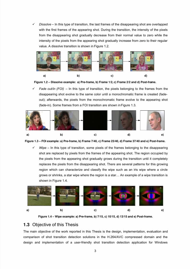
Dissolve – In this type of transition, the last frames of the disappearing shot are overlapped
with the first frames of the appearing shot. During the transition, the intensity of the pixels
from the disappearing shot gradually decrease from their normal value to zero while the
intensity of the pixels from the appearing shot gradually increase from zero to their regular
value. A dissolve transition is shown in Figure 1.2.
a) b) c) d)
Figure 1.2 – Dissolve example: a) Pre-frame, b) Frame 1/2, c) Frame 2/2 and d) Post-frame.
Fade out/in (FOI) – In this type of transition, the pixels belonging to the frames from the
disappearing shot evolve to the same color until a monochromatic frame is created (fade-
out); afterwards, the pixels from the monochromatic frame evolve to the appearing shot
(fade-in). Some frames from a FOI transition are shown in Figure 1.3.
a) b) c) d) e)
Figure 1.3 – FOI example: a) Pre-frame, b) Frame 7/40, c) Frame 23/40, d) Frame 37/40 and e) Post-frame.
Wipe – In this type of transition, some pixels of the frames belonging to the disappearing
shot are replaced by pixels from the frames of the appearing shot. The region occupied by
the pixels from the appearing shot gradually grows during the transition until it completely
replaces the pixels from the disappearing shot. There are several patterns for this growing
region which can characterize and classify the wipe such as an iris wipe where a circle
grows or shrinks, a star wipe where the region is a star… An example of a wipe transition is
shown in Figure 1.4.
a) b) c) d) e)
Figure 1.4 – Wipe example: a) Pre-frame, b) 7/15, c) 10/15, d) 13/15 and e) Post-frame.
1.3 Objective of this Thesis
The main objective of the work reported in this Thesis is the design, implementation, evaluation and
comparison of shot transition detection solutions in the H.264/AVC compressed domain and the
design and implementation of a user-friendly shot transition detection application for Windows
3

8/14/2019 H.264 Compressed Shot Detection
http://slidepdf.com/reader/full/h264-compressed-shot-detection 24/128
environments. Operating in the H.264/AVC compressed domain means that, the algorithm must only
perform some essential and low-complexity decoding tasks, like parsing the bit stream or do some
minor calculations, while avoiding all the time consuming decoding tasks, e.g., motion vectors inferring
or transform decoding.
To encourage research on information retrieval by providing a large test collection and uniform scoringprocedures, the Text Retrieval Conference (TREC) series has been initiated in 1992. In 2001, a video
"track" devoted to research on automatic segmentation, indexing and content-based retrieval of digital
video was initiated and, in 2003, an independent TREC Video Evaluation (TRECVID) conference
series [7] was formed. Between 2001 and 2007, the TREC and later the TRECVID initiatives provided
a common video database and common evaluation criteria with the associated ground truth, which
allowed evaluating several proposed shot transition detection systems under solid and fair conditions.
This contest environment had a major impact on the development of this technology.
Among the various metrics relevant for the evaluation of shot transition detection systems, the most
commonly used are:
o Recall – Ratio between the number of correctly detected shots and the number of existing shots
in the video material (1).
(1)
o Precision – Ratio between the number of correctly detected shots and the number of detected
shots (2).
(2)
These metrics will be also intensively used in this document to evaluate the performance of the
developed shot transition detection systems. In Figure 1.5 and Figure 1.6, the performance of the
participant teams in TRECVID 2007 is shown. These figures provide an idea on the precision and
recall values obtained nowadays with state-of-the-art shot transition technology. It is, however, very
important to remind that most of these algorithms work in the uncompressed domain and only a few of
them operate in the MPEG-1 compressed domain. The algorithms to be studied, designed,
implemented and evaluated in this Thesis make one step further since they work in the compressed
domain of the most recent video coding standard, the H.264/AVC.
1.4 Outline of this Thesis
This Thesis is organized in seven chapters besides this introductory chapter, where, mostly, the
motivation and objectives are presented. In 0, a short overview of the H.264/AVC video coding
standard is presented. In Chapter 3, a review of the state of the art on shot transition detection
systems is presented; with this review in mind, a general framework, and a classification tree for these
systems are also proposed; finally, some of the most representative shot transition detection systems
in the literature are reviewed. In Chapter 4, the architecture and the functional modules of the
developed shot transition detection systems are introduced. Next, a detailed description of the shot
transition detection algorithms designed and implemented for the core architectural modules is
4

8/14/2019 H.264 Compressed Shot Detection
http://slidepdf.com/reader/full/h264-compressed-shot-detection 25/128
provided in Chapter 5. In Chapter 6, the implementation and Graphical User Interface (GUI) of the
developed shot transition detection application are presented while, in 0, the video collection,
evaluation procedures and results of the tests performed with the developed shot transition detection
systems are presented. Finally, Chapter 8 presents the main conclusions of the Thesis and the
eventual future work.
Figure 1.5 – Performance results for abrupt transition detection obtained by the participant teams inTRECVID 2007 [7].
Figure 1.6 – Performance results for gradual transition detection obtained by the participant teams in
TRECVID 2007[7].
5

8/14/2019 H.264 Compressed Shot Detection
http://slidepdf.com/reader/full/h264-compressed-shot-detection 26/128
6

8/14/2019 H.264 Compressed Shot Detection
http://slidepdf.com/reader/full/h264-compressed-shot-detection 27/128
CHAPTE
Short Overview on the
H.264/AVC Video Coding
Standard
R 2
which specifically targets H.264/AVC compressed video material
considering its growing popularity.
p of the International Telecommunication Union Telecommunication Standardization Sector (ITU-
efficiency in comparison to any existing video coding standard for abroad variety of applications [8].
In this chapter, a short overview on the H.264/AVC standard is presented. This overview is intended to
provide the reader with the fundamental concepts and tools adopted in this standard, especially those
assuming a major role in this Thesis
2.1 Objectives and Architecture
The H.264/AVC standard is the latest international video coding standard [6], [8]. This standard is the
result of a partnership, known as the Joint Video Team (JVT), between the Moving Picture Experts
Group (MPEG), a working group of the International Organization for Standardization/International
Electrotechnical Commission (ISO/IEC), and the Video Coding Experts Group (VCEG) a working
grou
T).
In recent years, video coding has evolved through various standards (H.261 [9], MPEG-1 Video [10],
MPEG-2 Video [11], H.263 [12] and MPEG-4 Visual [13]) which aim at exploiting the research
advances achieved in video compression to provide support for video data in different applications and
networks. The main objective of this new standard was to develop a video coding standard which
should double the compression
7

8/14/2019 H.264 Compressed Shot Detection
http://slidepdf.com/reader/full/h264-compressed-shot-detection 28/128
The typical video encoding/decoding chain is shown in Figure 2.1. Like for the previous standards, the
H.264/AVC standard only standardizes the syntax and semantics of the bit stream as well as the
decoding process which must be performed to generate the decoded video. These restrictions are
applied to achieve interoperability and are as limited as possible to allow competition between different
manufactures in the remaining blocks of the encoding/decoding chain, such as more efficientencoders or more error resilient decoders.
Figure 2.1 –Typical video encoding/decoding chain and scope of the H.264/AVC standard [14].
The H.264/AVC standard is composed of two layers as depicted in Figure 2.2:
o Video Coding Layer (VCL) – This layer defines the efficient representation of the video data.
o Network Adaptation Layer (NAL) – This layer provides “network friendliness” by converting
the VLC stream into a format more suitable for storage or transmission.
Figure 2.2 – H.264/AVC network adaptation layer [14].
2.2 Video Coding Layer
In Figure 2.3, the encoding process of a frame is depicted; as in previous standards, the VCL splits the
luminance and chrominance samples of each frame into blocks, the so-called macroblocks. To
efficiently encode each macroblock, a prediction is made for the samples in each macroblock. To
generate this prediction, the macroblock can be split into smaller blocks which are called prediction
blocks. The encoder generates the bit stream containing the required information so that the decoder
can generate the same prediction and the so-called prediction error, which is the difference between
8

8/14/2019 H.264 Compressed Shot Detection
http://slidepdf.com/reader/full/h264-compressed-shot-detection 29/128
the actual original samples and the prediction. There are two major encoding prediction modes
defined in the H.264/AVC standard:
o Intra Mode – The prediction can be only based on samples from the current frame.
o Inter Mode – The prediction for each prediction block is based on samples taken from, at most,
two previously decoded frames which can, in visualization order, precede (forward prediction) or
succeed (backward prediction) the current frame. For this purpose, two lists of reference frames
are maintained: i) list0 which is usually used for forward prediction, and ii) list1 which is usually
used for backward prediction; these lists define the frames that can be used for reference in the
prediction. The prediction may be based on blocks in a different spatial position and, therefore,
at least one motion vector is needed to indicate the displacement of the reference block;
however, the number of motion vectors may significantly grow for more complex prediction
modes.
Entropy
Coding
Scaling & Inv.Transform
Motion
Compensation
Control
Data
Quant.
Transf. coeffs
Intra
Prediction
Data
Intra/Inter
MB select
Coder Control
Motion
Estimation
Transform/
Scal./Quant.-
InputVideo
Signal
Split into
Macroblocks
16x16 pixels
Intra-frame
PredictionDeblocking
Filter
Output
VideoSignal
Intra-frame
Estimation
Motion
Data
Figure 2.3 – Simplified H.264/AVC encoding architecture [8].
In previous standards, such as MPEG-2 Video [11], the video sequences are formed by a sequence of
successive independent coding structures called Group of Pictures (GOP). The GOPs specify the
order in which intra frames, which are independently decoded frames, and inter frames, which contain
motion compensation information, are arranged. Each GOP is formed by frames which can be of three
different types:
o I-Frames – Intra frames which can be independently decoded from other frames and mark the
beginning of each GOP.
o P-Frames – Predictive frames which contain motion-compensated difference information from
the preceding I- or P-frame; this allows the encoder to exploit temporal redundancy between the
reference and current frames.
9

8/14/2019 H.264 Compressed Shot Detection
http://slidepdf.com/reader/full/h264-compressed-shot-detection 30/128
o B-Frames – Bi-predictive frames which contain difference information from the preceding and
following I- or P-frame; B frames thereby allow the encoder to exploit temporal redundancies
between the current B frame and the preceding and succeeding reference frames.
If regular, the GOP structure is typically defined by two parameters: N and M. The first parameter is
called the GOP length and corresponds to the number of frames in the GOP; the second parameter is
the number of frames plus 1 between reference frames (I or P frames). In the new H.264/AVC
standard, any frame can be marked as “used for reference” and added to the reference lists ( list0 used
by P and B frames and list1 used by B frames only). Every inter prediction block can use any frame
present in those lists. These differences are depicted in Figure 2.4.
Figure 2.4 – Differences in the typical GOP structures between previous standards and H.264/AVC.
This flexibility allows the creation of arbitrary coding structures and makes it possible to organize
pictures in the bit stream in multiple ways. Usually, this is used for the creation of hierarchical coding
structures which improve the coding efficiency and offer multi-layered temporal scalability in a straight-
forward way [15]. These structures consist on multiple layers which result in a coarse-to-fine structure.
A particular example of such structures is shown in Figure 2.5; in these structures, pictures can only
use as reference for motion compensation pictures from the same or lower layers and pictures from
the lower layer can only use as reference previous pictures in display order.
The decoding order is typically different from the visualization order; in fact, it is much more flexible
than in previous standards. Therefore, each frame has an associated picture order count (POC) which
is a number that identifies each frame and reflects the visualization order (visualization order is
achieved by sorting the frames in ascending order according to their POC).
Figure 2.5 - Hierarchical coding pattern with four temporal layers [16].
In the H.264/AVC standard, frames consist of one or more slices which are usually groups of
macroblocks, usually in raster scan order: The macroblocks from each slice can be parsed from the bit
10

8/14/2019 H.264 Compressed Shot Detection
http://slidepdf.com/reader/full/h264-compressed-shot-detection 31/128
stream without the need of any information from any other slice. In especial cases, e.g. to achieve
better error resistance, a Flexible Macroblock Order (FMO) may be used in which case the
macroblock order in the slice may differ. In the H.264/AVC standard, there are five types of slices: I, B,
P, SI and SP. The SI and SP slices are new regarding previous standards and target to solve network
transmissions problems; for this reason, only the remaining three types will be considered here:
o I-Slice – In this type of slices, the samples have to be encoded using the intra mode defined in
Section 2.2.1.
o P-Slice – In this type of slices, the macroblocks may be encoded in intra mode or in inter mode
where each prediction block may use up to one motion vector and reference index.
o B-Slice – In this type of slices, the macroblocks may be encoded in intra or inter prediction
mode where each prediction block may be encoded using at most two motion vectors and two
reference indexes.
For each macroblock, the encoder decides which type of prediction should be used to maximize thecoding efficiency. For this, it computes the prediction error, which is quantized and transformed; after,
it entropy codes the prediction error along with other information so that the decoder can recomputed
that prediction; the outcome of the entropy coder is the H.264/AVC bit stream.
There are two types of entropy coders which can be used in H.264/AVC: i) Context-Adaptive Variable
Length Coding (CAVLC), and ii) Context-Adaptive Binary Arithmetic Coding (CABAC). The CABAC
solution yields a more efficient coding although due to an increased complexity.
2.2.1 Intra Prediction
In previous standards, macroblocks encoded in intra mode did not have any prediction; however, in
this new standard, a prediction for an intra coded macroblock block may be computed based on
samples from already decoded neighbor macroblocks in the same slice. There are four of such intra
encoding modes used for luminance samples:
o Intra4x4 – Each block of 4 x 4 luminance samples in the macroblock is predicted using one of
the 9 prediction modes introduced in Figure 2.6.
Mode 7 – Vertical-LeftMode 7 – Vertical-Left Mode 8 – Horizontal-UpMode 8 – Horizontal-UpMode 5 – Vertical-RightMode 5 – Vertical-Right Mode 6 – Horizontal-DownMode 6 – Horizontal-Down
Mode 0 - VerticalMode 0 - Vertical Mode 1 - HorizontalMode 1 - Horizontal Mode 3 – Diagonal Down/LeftMode 3 – Diagonal Down/Left Mode 4 – Diagonal Down/RightMode 4 – Diagonal Down/RightMode 2 - DC
++
+
+ + ++
Mode 2 - DC
++
+
+ + ++
Figure 2.6 - Intra4x4 prediction modes.
11

8/14/2019 H.264 Compressed Shot Detection
http://slidepdf.com/reader/full/h264-compressed-shot-detection 32/128
o Intra8x8 – In this intra mode, each 8 x 8 luminance block in the macroblock is predicted using
one of 9 prediction modes available which are similar to those in the Intra4x4 mode considering
8 x 8 blocks instead of 4 x 4 blocks.
o Intra16x16 – This mode performs macroblock predictions over the 16 x 16 samples macroblock
using one of the 4 prediction modes available and depicted in Figure 2.7.
Figure 2.7 - Intra16x16 prediction modes.
o PCM – This is a mode which is rarely used since it provides no compression when compared to
the previously introduced intra prediction modes; it is specified for the following purposes:
It allows the encoder to precisely represent the sample values.
It provides a way to accurately represent the values of anomalous picture content without
significant data expansion.
It enables placing a hard limit on the number of bits a decoder must handle for a
macroblock without harming the coding efficiency.
For chrominance samples, the macroblock is not divided and a prediction is made for all the 16x16 or
8x8 chrominance samples in the macroblock, depending on the chrominance sub-sampling format
used, e.g. 4:2:0 or 4:4:4. This prediction is made in the same fashion as Intra16x16, since
chrominance data is usually smooth over large areas.
2.2.2 Inter Prediction
Using the inter prediction mode, the prediction for a macroblock can be based on samples from other
previously decoded frames. The available prediction types to encode a macroblock depend on theslice type. The available inter prediction modes are explained in the following:
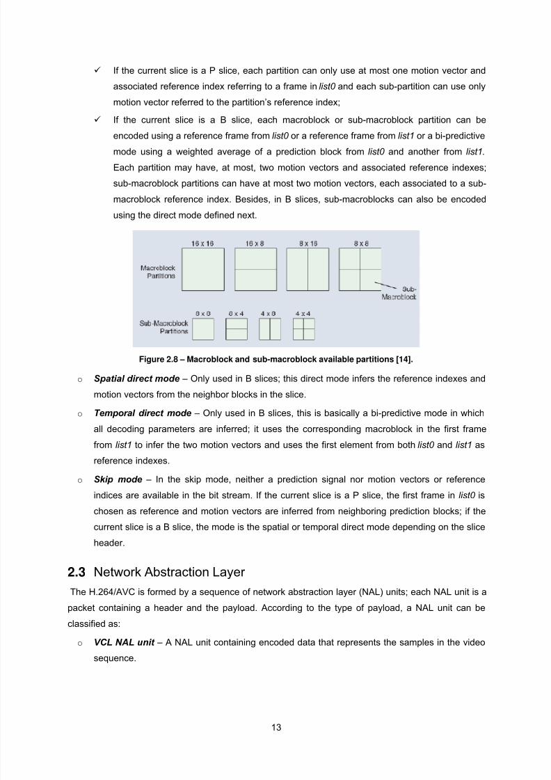
o P mode – In this mode, both the motion and prediction error information are available in the bit
stream. To maximize the coding efficiency, the H.264/AVC standard specifies several
partitioning modes for an inter macroblock, as depicted in Figure 2.8. Each H.264/AVC partition
can have its own motion information (motion vectors and associated reference indexes); in the
case of sub-macroblocks, which is the name given to 8x8 partitions of an P-mode macroblock,
besides the partition motion information, each sub-macroblock partition also can have its own
motion vector information. Depending on the slice type, this motion information can be of two
types:
12
8/14/2019 H.264 Compressed Shot Detection
http://slidepdf.com/reader/full/h264-compressed-shot-detection 33/128
If the current slice is a P slice, each partition can only use at most one motion vector and
associated reference index referring to a frame in list0 and each sub-partition can use only
motion vector referred to the partition’s reference index;
If the current slice is a B slice, each macroblock or sub-macroblock partition can be
encoded using a reference frame from list0 or a reference frame from list1 or a bi-predictive
mode using a weighted average of a prediction block from list0 and another from list1.
Each partition may have, at most, two motion vectors and associated reference indexes;
sub-macroblock partitions can have at most two motion vectors, each associated to a sub-
macroblock reference index. Besides, in B slices, sub-macroblocks can also be encoded
using the direct mode defined next.
Figure 2.8 – Macroblock and sub-macroblock available partitions [14].
o Spatial direct mode – Only used in B slices; this direct mode infers the reference indexes and
motion vectors from the neighbor blocks in the slice.
o Temporal direct mode – Only used in B slices, this is basically a bi-predictive mode in which
all decoding parameters are inferred; it uses the corresponding macroblock in the first frame
from list1 to infer the two motion vectors and uses the first element from both list0 and list1 as
reference indexes.
o Skip mode – In the skip mode, neither a prediction signal nor motion vectors or reference
indices are available in the bit stream. If the current slice is a P slice, the first frame in list0 is
chosen as reference and motion vectors are inferred from neighboring prediction blocks; if the
current slice is a B slice, the mode is the spatial or temporal direct mode depending on the slice
header.
2.3 Network Abstraction Layer
The H.264/AVC is formed by a sequence of network abstraction layer (NAL) units; each NAL unit is a
packet containing a header and the payload. According to the type of payload, a NAL unit can be
classified as:
o VCL NAL unit – A NAL unit containing encoded data that represents the samples in the video
sequence.
13

8/14/2019 H.264 Compressed Shot Detection
http://slidepdf.com/reader/full/h264-compressed-shot-detection 34/128
o Non-VCL NAL unit – A NAL unit containing additional information such as parameter sets.
These parameter sets contain information which supposedly rarely changes and is useful for
decoding a large number of NAL units. There are two of such parameter sets:
Sequence parameter set – This applies to a series of consecutive sequences of coded
video pictures called a coded video sequence.
Picture parameter set – This applies to the decoding of one or more individual pictures
within a coded video sequence.
A set of NAL units in a certain order containing one encoded picture is called an access unit. There is
a special type of access unit used at the beginning of each coded video sequence called
Instantaneous Decoding Refresh (IDR) unit. This IDR access unit contains an intra frame which can
be decoded without the need of decoding any previous image and indicates that no subsequent
picture will make reference to pictures prior to the intra picture it contains. Due to these properties, the
IDR unit marks the beginning of the GOP equivalent in the H.264/AVC standard.
2.4 Profiles and Levels
As referred earlier, the H.264/AVC standard was proposed to be used for a wide range of applications,
bit rates, resolutions, qualities and services. For that reason, the requirements for each of the relevant
applications were considered, namely, the balance between the required functionalities, like
compression efficiency, low delay and encoding/decoding complexity. To provide interoperability while
limiting the complexity, the H.264/AVC standard defines profiles and levels as already done in
previous video coding standards.
A profile is a subset of the coding tools defined in the standard. This way a decoder can implement
only one profile based on the requirements of the application for which it is being designed. Among the
profiles available, there are:
o Baseline profile – This is the simpler profile in encoding complexity but provides better error
concealment than the Main profile; it targets, for example, mobile video communications.
o Extended profile – Similar to the Baseline profile but with more tools, notably targeting
streaming applications.
o Main profile – Provides higher compression than the Baseline and Extended profiles; it targets
broadcasting applications.
o High profile – This is an extension of the Main profile providing more tools for high quality
applications.
Several levels are specified for each profile to constrain some values of the syntactic elements in the
bit stream, such as the number of reference pictures in the lists, the bitrate or the frame size. In fact,
given a certain profile, there is still a large variation in the decoding complexity since a profile only
fixes the tools used but not the amount of data in terms of sample and bits; therefore, since it is not
always practical or economical to implement a decoder to cope with every possible use of a profile,
this second profiling dimension was needed.
14

8/14/2019 H.264 Compressed Shot Detection
http://slidepdf.com/reader/full/h264-compressed-shot-detection 35/128
CHAPTE
State-of–the-Art Review on
Shot Transition Detection
R 3
posed first.
After, some of the most relevant shot transition solutions in the literature will be reviewed.
udy of shot
tation using an appropriate feature extraction
tion and classification of the transitions as hard cuts
The main purpose of this chapter is to provide a brief review on the shot transition detection
techniques available in the literature. In order this review has a more structured context, a general
shot transition detection framework and a classification tree for the various tools are pro
3.1 General Framework for Shot Transition Detection
After reviewing many algorithms on shot transition detection, a general framework could be abstracted
for shot transition detection algorithms at large; this general framework is presented in Figure 3.1. The
framework here proposed was mainly inspired by Yuan et al. [2] who made a formal st
transition detection where shot detection is generally described as a three steps process:
o Representation of visual content – The first step regards the extraction of features from each
frame to obtain a compact content represenmethod to map the image into a feature space;
o Construction of continuity signal – The second step regards the determination of a continuity
(similarity) or discontinuity (difference) signal between feature mappings for different frames;
o Classification of continuity values – Given the continuity signal representing content
variations, the final step regards the detec
or as various types of gradual transitions.
The main addition to this model was the introduction of a module operating independently from the
main processing chain described above – camera operation recognition – which, in some cases, is
15

8/14/2019 H.264 Compressed Shot Detection
http://slidepdf.com/reader/full/h264-compressed-shot-detection 36/128
used to provi re aiding the
detection task.
de important information about the visual content being analyzed, therefo
Figure 3.1 - General framework for shot transition detection algorithms.
In the proposed general framework, shown in Figure 3.1, several modules can be identified:
o Feature extraction – In this first stage, the visual content, available in a compressed or
uncompressed format, is represented by means of feature descriptors which map each frame
into a feature space in order further processing may be simplified. The extracted features, and
corresponding descriptors, should be sensitive enough to various content variations, thus
providing some additional
allowing a shot transition to be detected; during a shot, they should be invariant, in order no
false transitions are declared.
o Similarity score calculation – In the second module, descriptors are evaluated to measure the
similarity or dissimilarity (difference) between frames, thus generating continuity or discontinuity
scores. This may be achieved by simply analysis one or two frames, or by considering more
frames, thus incorporating contextual information into the process. Other scores may also begenerated in this module, which may aid the decision process by
16

8/14/2019 H.264 Compressed Shot Detection
http://slidepdf.com/reader/full/h264-compressed-shot-detection 37/128

8/14/2019 H.264 Compressed Shot Detection
http://slidepdf.com/reader/full/h264-compressed-shot-detection 38/128
purposes mentioned above, this means to have a more organized perspective on the type of solutions
available, the classification tree does not have to be unique.
Figure 3.2 - Proposed classification for shot transition detectors.
etectors are classified as discriminative,
sus compressed video content – The second classification dimension
mension, the spatial granularity of the generated feature frame descriptors is
The proposed classification tree classifies and clusters the algorithms according to three main
characteristics:
o Generic versus discriminative transition detector – As it has been stated in Chapter 1, there
are several types of transitions used in video editing; therefore, different approaches to their
detection might be used, which makes this first classification dimension very important and
appropriate. In this context, algorithms are classified according to its design as i) general, if they
detect shot transitions regardless of the transition type, or ii) discriminative if otherwise they
target a certain types of transitions. Since this classification exercise is more based on
conceptual resemblances than on implementation purposes, algorithms which try to detect all
types of transitions assembling together various d
because they rely on a discriminating approach to the problem, thus are more similar to
discriminative detectors rather than to general ones;
o Uncompressed ver
regards whether the algorithm is designed to work on uncompressed or compressed data, e.g.,
MPEG coded data.
o Single spatial granularity versus combination of spatial granularities – In the last
classification di
considered. The descriptors may be generated on a single level, e.g. frame, block or pixel, or on
various levels.
18

8/14/2019 H.264 Compressed Shot Detection
http://slidepdf.com/reader/full/h264-compressed-shot-detection 39/128
In the following, some further considerations are presented regarding the various classes of shot
algorithms is usually lower than the one provided by discriminative detectors. A more usual approach
ed by cascading a cut detector with a gradual
ot constrained to a specific
encoding format nor to a specific encoder implementation, so these detectors have greater detection
tent is coded, these algorithms will need the data to be decoded first,
putational resources, since the feature vectors generated might be
very large. For that reason, it is usually used in combination with less sensitive feature
ch – Another possibility is to segment each frame into blocks and extract
features for each block. Features extracted in this way have the advantage of being more
o
ose an algorithm creating a color histogram for each frame;
the descriptor uses singular value decomposition over a feature matrix formed by several
transition detectors resulting from the classification dimensions introduced above.
3.2.1 Generic Transition Detectors
In this class, the algorithms detect the transitions regardless of their type, e.g., abrupt and gradual.This approach is mainly used when a low complexity algorithm is required, since the alternative
usually corresponds in cascading discriminative detectors, thus increasing the processing time. They
are designed so the general characteristic of a shot transition is detected, that is, a significant
difference between a frame from a shot and the one belonging to the next shot. However, this type of
very general technique is not much used because the detection performance achieved by such
to detect all transition types is to use a detector design
transition detector [2], [20], which as explained earlier, is classified here as a discriminative solution.
3.2.1.1 Uncompressed Domain Detectors
Most of the literature presents algorithms based on features extracted from a raw image, this means
uncompressed data. The advantage of these algorithms is that they are n
potential. However, if the con
thus adding time-consuming computational complexity to the process.
Single Granularity Level
The uncompressed features can be obtained at various spatial granularity levels, notably:
o Pixel-based approach – Some shot transition algorithms exploit a feature descriptor
representing each pixel. This type of mappings is usually very sensitive to shot transitions;
however, it can also be extremely sensitive to motion, local changes and camera operation, and
usually requires more com
descriptors, for instance those taken on a frame or block basis, or with some kind of motion
compensation or filtering.
o Block-based approa
invariant to camera or object movement and local changes, without a significant loss in terms of
feature sensitivity.
Whole frame approach – Some algorithms use descriptors that describe whole frame features,
therefore being even more robust to motion within a shot than block-based solutions. However,
these approaches are usually less sensitive to shot changes since they might not consider the
spatial differences between compared frames. An example of this type of detector is proposed
in [21] where Cernekova et al. prop
19

8/14/2019 H.264 Compressed Shot Detection
http://slidepdf.com/reader/full/h264-compressed-shot-detection 40/128
column descriptors taken from successive frames and, afterwards, applies a dynamic clustering
ploys an unsupervised 2-feature, 2-means clustering using for
based descriptors (color histogram at the frame
eo is already available in the compressed domain, performing shot change
er a simple partial decompression offers obvious
Features which are directly available from the encoded bit stream or require
tions, such as motion vectors or block averages (DC transform
Level
nding on the coding standard used and the block hierarchy
s are available. The compressed features which can be extracted from
:
o
method to identify the transitions.
Combination of Spatial Granularities
A common approach to improve the detection performance is to adopt a similarity evaluation by
combining complementary descriptors taken at various spatial granularities. Naphade et al. [17]
propose an algorithm which em
comparison both pixel (pixel intensities) and frame-
level) to detect shot boundaries.
3.2.1.2 Compressed Domain Detectors
Uncompressed domain algorithms typically achieve very good results (see Chapter 1); however, since
most of the digital vid
detection directly on the compressed bit stream or aft
advantages, such as:
o Savings on decompression time and storage ;
o Faster operations due to the lower data rate;
o Existence of
relatively simple calcula
coefficients).
Single Granularity
As in the uncompressed domain, the compressed domain features might be extracted at variousspatial granularities:
o Block-based approach – In the compressed domain, pixel intensities are not directly available
in the bit stream, since pixel intensities are usually encoded into transform coefficients on a
block basis (see all MPEG video coding formats). The block from which features are extracted
may vary in size and shape depe
level where the feature
blocks more frequently used are
Motion vectors;
Transform coefficients;
Macroblock prediction types;
Whole frame approach – A common approach in compressed domain algorithms is to either
use features extracted from the whole frame, like the frame bit rate, or features available at the
block level to generate a frame descriptor, such as a frame histogram describing the transform
coefficients. In [22], Lelescu et al. propose a detector to work on MPEG-2 coded video, although
the authors claim this detector to be easily extendable to other compression formats. In this
algorithm, DC images, which are spatially reduced images formed by the DC coefficients
available for each block, for I and P coded frames are extracted and evaluated by a principal
20

8/14/2019 H.264 Compressed Shot Detection
http://slidepdf.com/reader/full/h264-compressed-shot-detection 41/128
component analysis (PCA). The algorithm models video sequences as stochastic processes,
nsition Detectorsnds of transitions, e.g., hard cuts and
n type;
nation in
gorithms that detect both abrupt and gradual transitions butin different stages.
more present in the literature than the generic ones.
S l
As fo
uncomp
o not a common approach due to its
poor invariance along frames from the same shot. In [23], Cernekova et al. propose an
o
g whole frame descriptors, the proposed wipe detection is
accomplished by calculating the mean square error using the mean and variance of each pixel
o
ch to detect dissolves and fades and it is oftensuggested to identify gradual transitions. For example, in [24], fades and dissolves are detected
thus detecting shot changes as changes in the parameters of the process, estimated in a
training process performed at the beginning of each shot.
3.2.2 Discriminative TraThis type of algorithms is designed to identify discriminative ki
dissolves, taking advantage of the specific characteristics of each transition type. There are various
types of such algorithms, notably:
o Those designed for detecting only one kind of transition;
o Those which are projected to detect a finite number of transitions types, usually built using a
detector per transitio
o Those which attempt to identity any type of transition but make some kind of discrimi
the processing stage, for example al
This type of solutions is by far
3.2.2.1 Uncompressed Domain
ing e Granularity Level
r generic algorithms, also in the case of discriminative algorithms, which operate in
ressed bit stream, the solutions may be clustered regarding their feature spatial granularity:
Pixel-based approach – As for general detectors, this is
algorithm for detecting shot boundaries which fits in this category. The detector tries to find cuts
by evaluating mutual information between two successive frames and fades by examining both
mutual information and the joint entropy over the transition.
Block-based approach – The main difference between this approach and the one presented
for general transition detectors is that the algorithms in this class model the variations in the
visual content induced by each kind of transition and then identify them separately. In [24],
Fernando et al. propose an algorithm to detect cuts, dissolves, fades and wipes by evaluating
intensity features for a statistical image, i.e. a reduced image where each pixel corresponds to
the mean and variance of the original pixels associated. Although cut, fade and dissolve
detectors are designed usin
which make up the statistical image, identifying those which have significant changes and
generating a binary image. Afterwards, the Hough transform is used to identify strips which
indicate some kinds of wipes.
Whole frame approach – In this discriminative class, features are processed on a frame basis.
Besides hard cuts, this is also a common approa
21

8/14/2019 H.264 Compressed Shot Detection
http://slidepdf.com/reader/full/h264-compressed-shot-detection 42/128
by evaluating the first and second order differences of the frame intensity variance and mean. In
gorithm to detect linear transitions, which can be either abrupt or gradual, by
isons into a linear transition model. The descriptors used are a
omain
Al i
bound
Singl
o
block differences between successive frames for cut
etector,
both block and frame basis. The two descriptors
nd the edge strength
both intensity histogram
representative review is
obtained. In this context, first, an algorithm working on the uncompressed domain is presented,
[20], gradual transitions are detected by evaluating the fitting error of the similarity signal
calculated regarding a gradual transition model.
Combination of Spatial Granularities
There are also discriminative algorithms which combine features taken at different spatial granularities
to improve performance. One example of such kind of algorithms is presented in [5]. In this paper,
Grana et al. suggest an al
fitting the multi-step inter-frame compar
frame intensity histogram and the pixel intensities which are employed later for the inter-frame
differences computation.
3.2.2.2 Compressed D
so n the compressed domain many discriminative solutions are available for the detection of shot
aries. They can be classified as follows:
e Level Granularity
Block-based approach – As suggested for many of the block-based algorithms, and according
to the authors, the algorithm described in [24] can also be applied to compressed streams, by
generating the statistical images from the available DCT coefficients. Another algorithm of such
kind is proposed by Hanjalic [3] where a cut detector is cascaded with a dissolve detector. The
author uses motion compensated
detection or between one frame and the twentieth next for detecting dissolves. The author also
suggests the design of other similar separate detectors which could join the cascade d
thus detecting more transition types.
o Frame-based approach – One detector belonging to this class is presented in [25]. This
detector analyses the correlation of the histogram difference vectors for wipe detection.
Combination of Spatial Granularities
In [26], Lee et al. present an algorithm for cut detection using the edge feature extracted directly from
DCT coefficients. The frame description is based on
are the edge orientation histogram, which describes the whole frame, a
histogram, which describes the edges on a block basis. Also, in [27] and [28]
and DC images are used to detect the transitions.
3.3 Main Relevant Shot Detection Transition Solutions
Since there are many techniques used for video shot transition detection, a brief review would not be
complete just by introducing a general framework and a classification tree for these algorithms.
Therefore, some recent solutions were chosen to be described in the next sections of this chapter: the
selection criteria for the solutions to be presented in the following, regarded their detection
performance and the coverage of the classes defined above, in order a
22

8/14/2019 H.264 Compressed Shot Detection
http://slidepdf.com/reader/full/h264-compressed-shot-detection 43/128
followed by an algorithm which works in the MPEG-1 video compressed domain; finally, three
discriminative, uncompressed and single level (block-
based) solutions. The authors submitted their detection performances to TRECVID 2005, 2006 and
s introduced for TRECVID 2007 [29] will
is
ntage of using this procedure is to
achieve invariance to local changes since the model incorporates significant contextual information.
fed to a Support Vector Machine (SVM) which tries to detect certain
The architecture of the solution presented in this section is shown in Figure 3.3; the highlighted blocks
ced in [29]. The detection is conducted by a hierarchical
ing the following steps described in the next section:
ection of cut transitions;
tion feature vectors;
o Motion post-processing;
o Scale Invariant Feature Transform (SIFT) post-processing.
algorithms operating in the H.264/AVC compressed domain are presented.
3.3.1 Shot Transition Detection Using a Graph Partition Model
In [2], from 2007, Yuan et al. present a formal study of the shot transition detection problem, reviewseveral of the existing technical approaches and, afterwards, present a shot transition detection
system based on a graph partition model (GPM). Finally, some experiments are conducted using the
TRECVID [7] platform, comparing various parameter profiles. Under the classification proposed in
Section 3.2, this system fits in the category of
2007, and obtained very good scores [7]. Some modification
be also considered in the following description.
3.3.1.1 Objectives and Basic ApproachThe main objective of this shot detection solution is to achieve a good performance in detecting any
kind of transition using a unified shot transition detector based on a graph partition model, which is
used to compute the similarity score signal.
An undirected weighted graph is used where the frames are treated as nodes while the weight of
edges expresses the similarity between the connected frames. At each time frame, a subset graph
divided into two sub-graphs by employing a min-max cut procedure with temporal constraints; the
obtained score is used as the continuity value. The main adva
The continuity signal is then
characteristic transition patterns usually present in video content.
3.3.1.2 Architecture
represent the modifications introdu
classification process consider
o Visual content representation;
o Fade out/in detection;
o Construction of continuity signal;
o Construction of feature vectors for cut detection;
o Training of the detector or det
o Construction of multi-resolu
o Gradual transition detection;
23

8/14/2019 H.264 Compressed Shot Detection
http://slidepdf.com/reader/full/h264-compressed-shot-detection 44/128
Figure 3.3 – Architecture of the graph partition model based detection algorithm [29].
3.3.1.3 Algorithm Description
A description of each module in the architecture presented in Figure 3.3 will be provided next:
Visual Content Representation
The descriptors used in this algorithm are block-based RGB histograms. In [2], the authors come to
the conclusion that the color scheme and the block size have little influence while detecting hard cuts
(although using RGB color space descriptors and larger blocks may yield slightly better
performances); however, they have much influence when detecting gradual transitions, where the best
results were obtained using 2 x 2 blocks. For that reason, 2 x 2 blocks were used in [2] while, in [29],
two block sizes were used to boost the detection results: 2 x 2 blocks for hard cut detection and 4 x 4
blocks for gradual transition detection.
Fade Out/in Detection
Due to the nature of fades, the corresponding continuity signal usually exhibits two valleys which, as
will be described later, might be detected as two transitions, using the cut and gradual transition
detectors. Therefore, a FOI detector is first executed. The implemented FOI detector consists on two
stages: i) monochrome frames detection; and ii) FOI location, both using the characteristics of mean
and standard deviation of pixel intensities.
24

8/14/2019 H.264 Compressed Shot Detection
http://slidepdf.com/reader/full/h264-compressed-shot-detection 45/128
Continuity Signal Construction
As stated earlier, the continuity signal is based on a graph partition model, which consists on dividing
one graph into parts. Two scores can be obtained: the cut , sum of weights connecting different parts,
and association, sum of weights connecting nodes in the same part. For this purpose, an undirected
weighted graph, like the one presented in Figure 3.4, is created along with a similarity matrix which
holds the edge weights reflecting the node similarities.
Figure 3.4 - Graph with 13 nodes (left) and similarity matrix (right) where bright means high similarity asopposed to dark [2].
These similarities are computed using a modified histogram intersection method (3) over the
descriptors created in previous stages (between the corresponding blocks in the images) and, then,
the obtained block similarities are summed together to generate the frame similarities. At each time
frame, a sub-graph of size d around the frame being inspected is divided in two using a min-max cut
procedure, which tries to minimize the cut while maximizing the association. The min-max cut score
obtained corresponds to the similarity score (st ) composing the continuity signal to be provided to the
detector.
, || , | | 0, (3)
Feature Vector Construction for Cut Detection
The input of the detector at each frame is a feature vector formed by 2r+1 successive continuity values
as indicated in (4).
),...,,,...,( 1 r t t t r t
r
t ssss B++−= (4)
In the case of a transition between frame t and frame t+1, this vector should be a regular and
symmetric valley with a local minimum at st , the time frame at which the transition occurs, as depicted
in Figure 3.5.
Training or Detecting Cuts (Cut SVM Classifier)
The detection method used in this algorithm is based on a SVM. To train the detector, the authors
annotated a training set consisting of negative and positive examples; however, since usually video
sequences are imbalanced due to the infinite negative examples, the training examples must be
carefully selected. For that reason, an active learning method is employed; the training set used
25
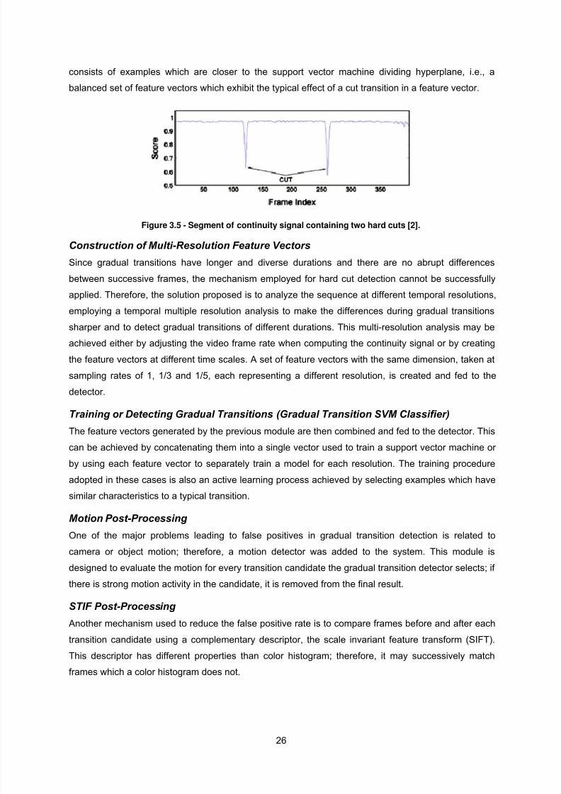
8/14/2019 H.264 Compressed Shot Detection
http://slidepdf.com/reader/full/h264-compressed-shot-detection 46/128

8/14/2019 H.264 Compressed Shot Detection
http://slidepdf.com/reader/full/h264-compressed-shot-detection 47/128
3.3.1.4 Performance Evaluation
The solution presented in this section has been extensively tested. In [2], the authors carry out several
experiments to evaluate alternative solutions for each major module. In TRECVID 2007, the algorithm
has been ranked among the best.
The TRECVID 2007 video set consisted of seventeen videos corresponding to 637,805 frames; 2,463
transitions; 2,236 cuts (90.8%); 134 dissolves (5.4%); 2 fade-out/-in (<0.1%); 91 other special effects
(3.7%). Ten runs, whose descriptions are available in Table 3.1, were submitted for evaluation in
TRECVID 2007, obtaining the results presented in Table 3.2.
Table 3.1 - Description of the ten runs evaluated in TRECVID 2007 [29].
Sysid Description
Thu01Baseline system : RGB histogram using 2 x 2 blocks for cut and gradual transition detector, no motiondetector, no sift post-processing, only using development set of 2005 as training set.
Thu02Same algorithm as thu01, but with 2 x 2 blocks for cut detector and 4 x 4 blocks for gradual transitiondetector
Thu03 Same algorithm as thu02, but with SIFT post-processing for cut detectionThu04 Same algorithm as thu03, but with Motion detector for GT
Thu05 Same algorithm as thu04, but with SIFT post-processing for GT
Thu06 Same algorithm as thu05, but no SIFT processing for CUT
Thu09 Same algorithm as thu05, but with different parameters
Thu11 Same algorithm as thu05, but with different parameters
Thu12 Same algorithm as thu05, but with different parameters
Thu13 Same algorithm as thu05, but with different parameters
Thu14 Same algorithm and parameters as thu05, but trained with all the development data from 2003-2006
Table 3.2 – Evaluation results for the ten submissions to TRECVID 2007 [29].
Sysid
All Transitions Cuts Gradual Transitions
Recall Precision Recall Precision Recall Precision
thu01 96% 88% 97% 96% 79% 41%
thu02 96% 88% 97% 97% 79% 41%
thu03 95% 89% 97% 98% 80% 41%
thu04 95% 94% 97% 98% 76% 62%
thu05 95% 96% 97% 98% 74% 70%
thu06 95% 94% 97% 97% 73% 69%
thu09 95% 96% 97% 98% 71% 70%
thu11 95% 96% 97% 98% 72% 73%
thu13 95% 96% 97% 98% 73% 69%
thu14 95% 96% 97% 98% 73% 69%
As stated earlier, this algorithm has presented performances which are among the best in successive
TRECVID evaluations. In TRECVID 2007, thu07 obtained 95% Recall and 96% Precision over all
transitions, 97% Recall and 98% Precision over hard cuts and 72% Recall and 73% Precision over
gradual transitions. Although the gradual transition detection performance is not impressive, one must
take into account that this algorithm has obtained very good results when compared to the other
evaluated algorithms; indeed, all algorithms seemed to perform worse in this task in TRECVID 2007
than they did in previous years [7].
27

8/14/2019 H.264 Compressed Shot Detection
http://slidepdf.com/reader/full/h264-compressed-shot-detection 48/128
3.3.2 Shot Transition Detection Based on a Statistical Detector
The next algorithm to be described in this review has been proposed by Hanjalic [3], in 2002, and can
be classified as a discriminative, compressed and single level (block-based) solution; it detects cuts
and dissolves in MPEG-1 coded video sequences.
3.3.2.1 Objectives and Basic Approach
In this solution [3], Hanjalic proposes a conceptual approach to the shot transition detection problem
making use of a statistical detector, a solution similar to the one previously adopted by Vasconcelos et
al. in [18], where the statistical detection theory is used for detecting shot boundaries. According to
Hanjalic, the main advantage of this solution is its robustness, that is, its capability to provide excellent
detection performance for different types of boundaries, and its rather constant detection performance
over any kind of video sequence, with minimized need for manual tuning of the detection parameters.
To achieve such robustness, this algorithm uses motion compensation to compute the similarity
between frames and also additional information based on a priori knowledge about the different types
of shot boundaries in video sequences.
3.3.2.2 Architecture
The basic architecture for the proposed statistical detector is presented in Figure 3.6.
Figure 3.6 - System architecture for the statistical detector [3].
In his algorithm, Hanjalic proposes using a module, like the one shown in Figure 3.6, for each
transition type. Although this particular algorithm is designed for the detection of cuts and dissolves,
the author claims to have introduced the general principles for the development of a statistical shot
change detector. Therefore, more discriminative similar detectors may be designed to detect other
transition types, by exploiting the characteristics of each type; they would be then linked together in a
cascade, as depicted in Figure 3.7.
3.3.2.3 Algorithm Description
As can be observed in Figure 3.6, this transition detection algorithm may be split in two main stages:
o Discontinuity computation – The distance between two frames (frame k and frame k + l ) is
computed, generating the discontinuity value z(k, k + l);
28

8/14/2019 H.264 Compressed Shot Detection
http://slidepdf.com/reader/full/h264-compressed-shot-detection 49/128
o Detector – The discontinuity values are evaluated and several scores, which embed the
additional information referred earlier, are computed to generate the decision about the
presence and type of transition.
Figure 3.7 - Detector cascade for detecting various transition types [3].
Discontinuity Computation
In this algorithm, the descriptors proposed are block-wise averages of the three components in the
YUV space. In the particular case of a MPEG compressed stream, as considered in this paper, a
partial decoding is done to extract DC images; the blocks are formed by averaging 4 x 4 pixels
squares of the DC images.
The discontinuity values are then computed as block differences with a block matching procedure.
Although the descriptors used already provide some invariance to motion, the motion compensation
employed in the distance computation stage provides an even more robust metric to evaluate
discontinuity values.
Due to the aforementioned differences between cuts and gradual transitions, in this particular case the
differences between cuts and dissolves, two discontinuity values are computed for each frame k . For
cut detection, these values are computed comparing successive frames, i.e., l = 1, whereas for
dissolve detection the aim is to compare frames from the beginning and the end of the transition;
therefore, l should be set to be largest than the minimum shot length ( l = 22 was taken for this
purpose). These discontinuity scores are shown in Figure 3.8.
Detector
The detector used in this solution employs the statistical detection theory to decide between two
hypotheses:
o Hypotheses : Existence of a transition between frames k and k + l ;
o Hypotheses : Non-existence of a transition between frames k and k + l .
A decision rule (5) is then derived which minimizes the average error probability. This decision rule
can be transformed into a simple expression like the one presented in Figure 3.6.
(5)
29

8/14/2019 H.264 Compressed Shot Detection
http://slidepdf.com/reader/full/h264-compressed-shot-detection 50/128
There are two types of entities ishabl decision ruledistingu e in the
o Likelihood functions ( | and (5):
) – They express the probability that a certain
discontinuity value has of belonging to each hypothesis. These functions are estimated using
several representative training sequences; they should not contain strong motion or strong
lighting changes because this might include discontinuity values which are out of their proper
range due to the effects of these extreme factors;
o P k (S) – It stands for the probability of validation of the hypotheses S at a frame k . This term (6)
reflects the influence of two kinds of information in the decision process:
( ) ( ) ( )( )k SPSPSPk
a
k k ψ |=
(6)
A priori information – Information that does not depend on any measurement on a
discriminative video sequence; in this algorithm, the author models the probability of a shot
transition occurring after a certain number of elapsed frames since the last detectedtransition, mainly to reduce false detections of shot boundaries detected immediately after
a previous one.
Additional information – Information which depends not only on initial assumptions but
also on the observed data. With this purpose, Hanjalic suggests using some pattern
modeling functions (ψ(k)) to compare the measured pattern within the temporal vicinities
(using a sliding window of size N ) of the frame being evaluated with the typical pattern
previously formulated for each transition type. This allows providing the detector with some
contextual information which might confirm, or contradict, the guess made by only
evaluating the distance functions for the frame under processing. The patterns which the
detector tries to identify are a sharp peak in the discontinuity values for cuts, and a
triangular pattern in the discontinuity values combined with an analysis on the intensity
variance along the frames in the sliding window for dissolves. This assumption can be
made by observation of the discontinuity values in Figure 3.8.
The terms in (6) and the likelihood functions are calculated and then the decision rule (5) is evaluated
successively in each module in the cascade until a transition is detected or the end of the cascade is
reached, in a process depicted in Figure 3.7.
3.3.2.4 Performance Evaluation
The performance of this algorithm has been evaluated by Hanjalic [3] for five test sequences,
belonging to four program categories (movie, football match, news and commercial documentary),
using the same detection parameters. These sequences, not used in the training stage in which
likelihood functions and other detection parameters were obtained, contain several effects which
usually cause detection errors, such as camera motion and zooming, fast object motion editing
effects... The performance evaluation results are shown in Table 3.3.
30

8/14/2019 H.264 Compressed Shot Detection
http://slidepdf.com/reader/full/h264-compressed-shot-detection 51/128

8/14/2019 H.264 Compressed Shot Detection
http://slidepdf.com/reader/full/h264-compressed-shot-detection 52/128
algorithms operating on previous MPEG standards, may be unfeasible (e.g. due to intra prediction).
Therefore, the solutions presented for shot detection on H.264/AVC use features available after the
very first decompression stage, this means entropy decoding. Another problem addressed by the
authors is the robustness of the algorithm to different encoding options; for example, the authors point
out that the algorithm in [35] has issues working with H.264/AVC Baseline profile streams since thisprofile only uses forward prediction.
To achieve the defined goals, the authors propose using difference scores based on the prediction
modes used by the encoder, notably:
o Intra macroblock proportion (IMBP) – If the inter prediction residual for a macroblock is too
high, the encoder will use intra coding for that macroblock, a situation that often occurs in a shot
change; this IMBP parameter express the ratio between the of intra coded macroblocks and all
macroblocks in a frame.
o Partition type count difference (PTCD) – There are several prediction block sizes in which
each macroblock can be divided. The partitioning is chosen by the encoder to minimize the
residual; therefore, similar partitioning is frequently used to encode successive frames within
slow-changing scenes whereas shot changes may result in significant changes in the
partitioning. This PTCD parameter expresses the differences in the partitioning used between
two frames.
3.3.3.2 Architecture
The architecture of the proposed algorithm is presented in Figure 3.9: it mainly consists of transition
detection modules using the IMBP or PTCD parameters and post-processing modules.
Figure 3.9 – Architecture of the shot detection algorithm [34].
3.3.3.3 Algorithm Description
A description of each module present in the architecture in Figure 3.9 is provided next:
Hard Transition (cut) Detection Based on PTCD
The successive prediction partitions chosen by the encoder may also be used to evaluate the
similarity between frames. Therefore, a partition histogram consisting of 15 bins is used to describe
each frame. Each bin represents a type of partition in a certain macroblock type; this descriptor uses
all partition types define by the standard, except those for intra macroblocks since, according to the
authors, these macroblocks in the partition histogram would produce many false alarms. To evaluate
the difference between successive frames, a weighted sum of differences between the corresponding
32

8/14/2019 H.264 Compressed Shot Detection
http://slidepdf.com/reader/full/h264-compressed-shot-detection 53/128
histograms is employed. A candidate frame is added to a candidate set of PTCD shot transitions if its
PTCD is higher than a predefined threshold (TH P ).
Gradual Transition Detection Based on IMBR
As stated earlier, the ratio of intra coded macroblocks may be taken as a sign of a shot transition. If a
shot transition occurs, the residual of a P or B macroblock may be too high and the encoder may use
intra coding instead. With this purpose, frames which have the IMBR over a predefined threshold ( TH I )
are added to the candidate set of IMBR shot transitions.
Shot Classification
In this module, the results in each candidate set are evaluated to distinguish gradual transitions from
hard cut transitions. If a gradual transition occurs, several consecutive candidates will be added to the
candidate set in the previous stages. In this module, such consecutive candidates, corresponding to a
gradual transition, will be grouped together and considered as a single gradual shot transition.
Furthermore, the PTCD approach works well for cut detection but performs poorly for gradual
transitions; meanwhile, IMBR works better for gradual transitions. Therefore, PTCD is used for cuts
and only gradual transitions are considered in the results obtained by the IMBR module.
Consecutive Cut Removal
Another post-processing step is the removal of candidate cuts which regard consecutive frames not
grouped into gradual transitions by the shot classification procedure.
Regular Intra Frame Detection
Those frames which were encoded in intra mode due to encoding constraints, namely GOP size, are
called Regular Intra Frames. These should be ignored since they generate false transition candidates.
To detect these regular intra frames, there are, thus, three possibilities:
o If the encoder is known, its default settings for Group of Pictures (GOP) size, i.e., distance
between intra frames, can be considered;
o If the entire bit stream is available, the dominant GOP size can be estimated;
o If the encoder is unknown and the entire bit stream is not available, the dominant GOP size can
be estimated using an incremental scheme.
3.3.3.4 Performance EvaluationIn [34], the authors present performance measurements for three video sequences:
o Video I: James Bond – Casino Royale movie trailer: 320x176 luminance resolution; 3650
frames; 169 transitions; 136 cuts (80.5%); 33 gradual transitions (19.5%).
o Video II: Sex-an-the-City, Season 1, Episode 1 (first 20 minutes): 352x288 luminance
resolution; 29836 frames; 231 transitions; 114 cuts (49.4%); 117 gradual transitions (50.6%).
o Video III: TRECVID2001-BOR03: 320x240 luminance resolution; 48451 frames; 242
transitions; 231 cuts (95.5%); 11 gradual transitions (4.5%).
The videos were encoded with the H.264/AVC Baseline profile using three popular encoders: Apple
QuickTime 7 Pro [36], x264 [37] and Nero Recode 7 [38].
33

8/14/2019 H.264 Compressed Shot Detection
http://slidepdf.com/reader/full/h264-compressed-shot-detection 54/128
The best results achieved by the algorithm in the experiments reported by the authors in [34], are
shown in Table 3.4. In Figure 3.10, the Recall and Precision scores obtained for video I using the Nero
encoder for different threshold values are shown; in Figure 3.11, similar scores are shown for the
QuickTime encoder. An additional performance measure is also used by the authors: the average shot
detection time in relation to the decoding time. This is important since the algorithm works oncompressed domain and, therefore, a significant reduction in the algorithm execution time may be also
a major requirement.
Table 3.4 - Best results obtained by the IMBR/PTCD detection approach [34].
Video THP/THI Detected
cuts/gradualsFalse
DetectionRecall Precision
Average shot detectiontime in relation to the
decoding time
I(Nero)
0.60/0.60 135/25 6 94% 96% 9.54%
II (QT) 0.50/0.60 112/108 14 95% 94% 8.41%
III(QT)
0.50/0.50 228/3 22 95% 91% 9.17%
Figure 3.10 – Recall and Precision for the IMBR/PTCD detection approach for video I (Nero) [34].
From the presented results, the authors concluded that the algorithm performance does not vary
significantly for the various encoders and sequences used; moreover, the thresholds do not need
great adjustments to achieve the best results for the different sequences and encoders. Also the
algorithm execution time is below 10% of the time required to decompress the video sequences.
Figure 3.11 - Recall and Precision for the IMBR/PTCD detection approach for video I (QT) [34].
Other tests carried out by the authors, however, have shown that IMBR is highly dependent on the
video encoding bit rate, generating more false alarms for the videos coded with higher bit rate.
Another possible problem referred is the behavior of the algorithm with other encoding profiles since it
34
8/14/2019 H.264 Compressed Shot Detection
http://slidepdf.com/reader/full/h264-compressed-shot-detection 55/128
has only been tested with sequences encoded with the Baseline profile, which uses fewer H.264/AVC
tools.
3.3.4 Shot Detection in H.264/AVC Hierarchical Bit Streams
In [16], from 2008, De Bruyne et al. present a shot detection algorithm operating in the H.264/AVCcompressed domain algorithm which detects both cuts and gradual transitions. Considering the
classification presented in Section 3.2, this is discriminative and compressed algorithm based on a
combination of feature granularities (frame and block levels).
3.3.4.1 Objective and Basic Approach
This algorithm relies on several features, some of which, contrary to the previous solutions, are not
available at the very first parsing level. While intra and inter prediction modes are used, as the
previous algorithms, the algorithm additionally recurs to motion information, which is not directly
available in the bit stream.
The authors propose two algorithms: one for shot transition detection for traditional coding patterns
and another for hierarchical coding structures such as those which may be used in the H.264/AVC
standard. The same features and difference scores are considered in the two algorithms; thus, the
main difference between these two algorithms is that while the first algorithm compares consecutive
frames, the second algorithm efficiently exploits hierarchical (or pyramidal) coding structures to speed
up the process, considering primarily frames from the base layer and, only when a shot change is
suspected to happen, processing frames from higher layers.
3.3.4.2 ArchitectureThe architecture of this algorithm is presented in Figure 3.12.
3.3.4.3 Algorithm Description
This algorithm detects both abrupt and gradual transitions. In this article, the authors proposed one
algorithm to abrupt transitions and another to detect gradual transitions, by analyzing the frames in the
video sequence. These procedures, for detecting each type of transitions, are described next and,
afterwards, the usage of these procedures, in the context of hierarchical coding structures, is
described.
Detection of Abrupt Transitions Relying on Temporal Dependencies
To detect an abrupt transition between two consecutive frames (in terms of global visualization order
or considering only frames of the same layer), temporal dependences in those frames are evaluated.
In fact, since a frame from a shot usually does not share similarities with a frame from the next shot,
the H.264/AVC encoder reflects that fact in the reference frames it uses to generate predictions.
Therefore, when an abrupt shot change occurs, the pre-frame is usually encoded using forward
predicted blocks, while the post-frame consists of intra or backward predicted blocks. In such case, it
is said that a gap in the temporal prediction chain has occurred, as illustrated in Figure 3.13, since this
behavior differs from that which is expected.
35
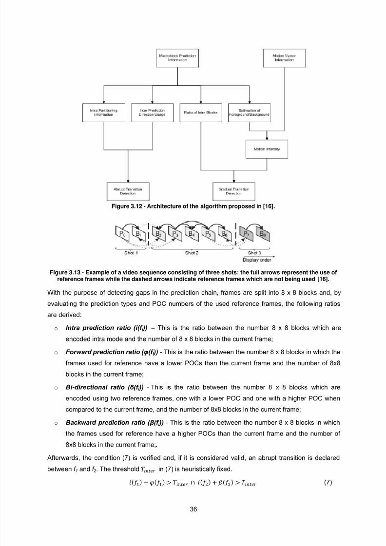
8/14/2019 H.264 Compressed Shot Detection
http://slidepdf.com/reader/full/h264-compressed-shot-detection 56/128
Figure 3.12 - Architecture of the algorithm proposed in [16].
Figure 3.13 - Example of a video sequence consisting of three shots: the full arrows represent the use ofreference frames while the dashed arrows indicate reference frames which are not being used [16].
With the purpose of detecting gaps in the prediction chain, frames are split into 8 x 8 blocks and, by
evaluating the prediction types and POC numbers of the used reference frames, the following ratios
are derived:
o Intra prediction ratio (i(f i )) – This is the ratio between the number 8 x 8 blocks which are
encoded intra mode and the number of 8 x 8 blocks in the current frame;
o Forward prediction ratio ( φ(f i )) - This is the ratio between the number 8 x 8 blocks in which the
frames used for reference have a lower POCs than the current frame and the number of 8x8
blocks in the current frame;
o Bi-directional ratio ( δ (f i )) - This is the ratio between the number 8 x 8 blocks which are
encoded using two reference frames, one with a lower POC and one with a higher POC when
compared to the current frame, and the number of 8x8 blocks in the current frame;
o Backward prediction ratio ( β(f i )) - This is the ratio between the number 8 x 8 blocks in which
the frames used for reference have a higher POCs than the current frame and the number of
8x8 blocks in the current frame;.
Afterwards, the condition (7) is verified and, if it is considered valid, an abrupt transition is declared
between f 1 and f 2 . The threshold
in is heuristical y fixed.
(7) l
(7)
36
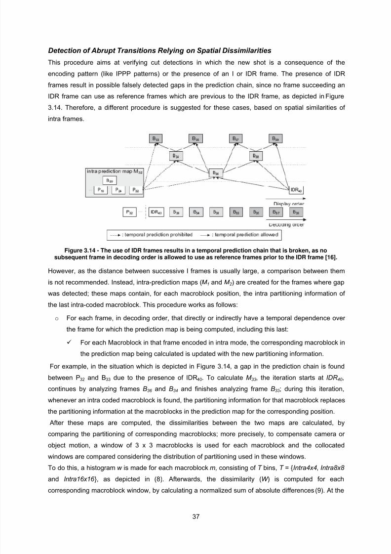
8/14/2019 H.264 Compressed Shot Detection
http://slidepdf.com/reader/full/h264-compressed-shot-detection 57/128
Detection of Abrupt Transitions Relying on Spatial Dissimilarities
This procedure aims at verifying cut detections in which the new shot is a consequence of the
encoding pattern (like IPPP patterns) or the presence of an I or IDR frame. The presence of IDR
frames result in possible falsely detected gaps in the prediction chain, since no frame succeeding an
IDR frame can use as reference frames which are previous to the IDR frame, as depicted in Figure
3.14. Therefore, a different procedure is suggested for these cases, based on spatial similarities of
intra frames.
Figure 3.14 - The use of IDR frames results in a temporal prediction chain that is broken, as nosubsequent frame in decoding order is allowed to use as reference frames prior to the IDR frame [16].
However, as the distance between successive I frames is usually large, a comparison between them
is not recommended. Instead, intra-prediction maps (M 1 and M 2 ) are created for the frames where gap
was detected; these maps contain, for each macroblock position, the intra partitioning information of
the last intra-coded macroblock. This procedure works as follows:
o For each frame, in decoding order, that directly or indirectly have a temporal dependence over
the frame for which the prediction map is being computed, including this last:
For each Macroblock in that frame encoded in intra mode, the corresponding macroblock in
the prediction map being calculated is updated with the new partitioning information.
For example, in the situation which is depicted in Figure 3.14, a gap in the prediction chain is found
between P32 and B33 due to the presence of IDR40. To calculate M 33, the iteration starts at IDR 40 ,
continues by analyzing frames B36 and B34 and finishes analyzing frame B33; during this iteration,
whenever an intra coded macroblock is found, the partitioning information for that macroblock replaces
the partitioning information at the macroblocks in the prediction map for the corresponding position.
After these maps are computed, the dissimilarities between the two maps are calculated, by
comparing the partitioning of corresponding macroblocks; more precisely, to compensate camera or
object motion, a window of 3 x 3 macroblocks is used for each macroblock and the collocated
windows are compared considering the distribution of partitioning used in these windows.
To do this, a histogram w is made for each macroblock m, consisting of T bins, T = {Intra4x4, Intra8x8
and Intra16x16 }, as depicted in (8). Afterwards, the dissimilarity (W ) is computed for each
corresponding macroblock window, by calculating a normalized sum of absolute differences (9). At the
37
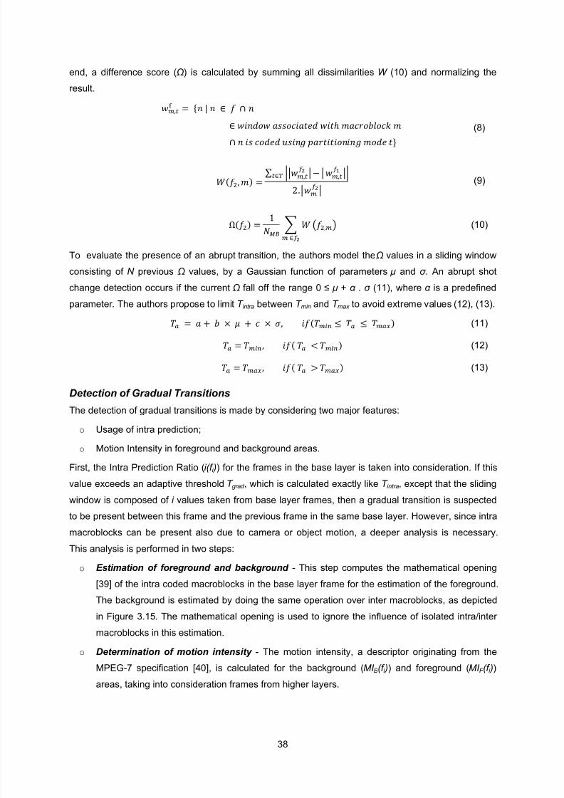
8/14/2019 H.264 Compressed Shot Detection
http://slidepdf.com/reader/full/h264-compressed-shot-detection 58/128

8/14/2019 H.264 Compressed Shot Detection
http://slidepdf.com/reader/full/h264-compressed-shot-detection 59/128
Figure 3.15 - Extraction of foreground and background using the mathematical morphology operationopening [16].
o Distinction between motion and gradual changes - If MI B(f i ) and MI F (f i ) are both high, the
presence of intra blocks can be attributed to camera motion; else, if only MI F (f i ) is high, this is
usually due to object motion. Otherwise, if both MI B(f i ) and MI F (f i ) are low, the presence of intra
blocks is due to a gradual transition and, therefore, a gradual transition is declared. The
threshold for classifying the motion as high/low is presented in (20), where x is a heuristically
set parameter, l stands for the diagonal length of the frame in pixels and F is the frame rate.
(14)
Algorithm for hierarchical coding structures
Hierarchical coding structures introduced in the H.264/AVC standard have some advantages over
regular coding structures, as referred in Section 2.2. To exploit these coding structures, the
procedures defined above, for detecting abrupt and gradual transitions, are tweaked. The authors
propose the identification of the hierarchical structure of a bit stream by relying on three supplemental
enhancement information (SEI) messages. SEI is a special type of non-VCL NAL units defined by the
H.264/AVC standard; these SEI messages assist in processes related to decoding, display or other
purposes and are not required for constructing the samples by the decoding process. However, these
are not always inserted by the encoder; in this case, a more complex analysis based on the decoding
and display order of the pictures is feasible to detect the hierarchical structures used.
For abrupt transitions, a recursive algorithm is used where the successive frames from the base layer
are first evaluated using the algorithm described earlier. If the process leads to an abrupt transition
detection, the higher layers are considered. This is done by dividing the segment between the two
frames from the base layer in two, one starting on the first base layer frame and ending on the midway
frame in the above layer and, the other, starting in this last frame and ending on the second frame
from the base layer. The procedure for detecting abrupt transitions is then repeated for each segment,
as depicted in Figure 3.16, until an abrupt transition between two consecutive frames is found. If an
abrupt transition is found due to the presence of an IDR frame, as in Figure 3.14, intra prediction maps
for the successive frames are created and compared to validate, or not, that detection.
39

8/14/2019 H.264 Compressed Shot Detection
http://slidepdf.com/reader/full/h264-compressed-shot-detection 60/128
Figure 3.16 - Recursive algorithm for detecting shot abrupt transitions in hierarchical structures [16].
For gradual transitions, the intra usage is calculated and evaluated considering base layer frames. If
the intra usage in a frame of the base layer is above T grad , the intra usage in the intermediate frame in
the next level is evaluated. If the intra usage in that frame is low, more precisely, if it is below a
predefined threshold (T nextLayer ), the motion intensity is calculated for that frame considering the
foreground and background estimated at the base layer. Otherwise, if the intra usage in that frame is
high, motion information from that frame is not reliable. Therefore, the procedure needs to be repeated
considering that as the base frame for extracting the foreground and background and motion
information is evaluated at the next layer. Unless this also uses to much intra prediction in which case
the procedure advances to the next layer and so on. This is exemplified in Figure 3.17; i(f 24) > Tgrad
which causes the previous frame in the above layer to be analyzed, in terms of its motion prediction.As this frame still has many intra coded blocks, i(f 22)>Tnextlayer , the motion analysis is performed on
frames f 21 and f 23 instead, where i(f 21)<Tnextlayer and i(f23)<Tnextlayer .
This hierarchical algorithm is summarized in Figure 3.18.
Figure 3.17 – Example of a gradual transition in a hierarchical coding structure. Intra-coded macroblocksare represented by their original color, whereas inter coded macroblocks are blanched [16].
40

8/14/2019 H.264 Compressed Shot Detection
http://slidepdf.com/reader/full/h264-compressed-shot-detection 61/128
Figure 3.18 - Flow chart of the algorithm proposed for the detection shot transitions on hierarchicalcoding patterns [16].
3.3.4.4 Performance Evaluation
In [16], the authors present performance measurements for five video sequences:
o News 1 – V3 video from the MPEG-7 Content Set; 352x288 luminance resolution; 26000
frames; 25 frames per second; 172 transitions; 154 cuts (89.5%); 18 gradual transitions
(10.5%).
o Basket – V17 video from the MPEG-7 Content Set; 352x288 luminance resolution; 18053
frames; 25 frames per second; 75 transitions; 62 cuts (82.7%); 13 gradual transitions (17.3%).
o News 2 – News broadcast from Belgium public television; 384x208 luminance resolution; 23802
frames; 25 frames per second; 157 transitions; 138 cuts (87.9%); 19 gradual transitions
(12.1%).
o Soap – Part of an international television soap; 720x576 luminance resolution; 15040 frames;
25 frames per second; 167 transitions; 160 cuts (95.8%); 7 gradual transitions (4.2%).
o Trailer – Little miss sunshine movie trailer; 848x352 luminance resolution; 3553 frames; 25
frames per second; 105 transitions; 81 cuts (77.1%); 24 gradual transitions (22.9%).
These sequences were encoded a number of times using different hierarchical coding patterns, with
two layers (hier_2), four layers (hier_4) and eight layers (hier_8). Besides, two versions of these
coding patterns were generated: one using I frames and the other using IDR frames, which were
inserted every 32 frames. The difference between these two solutions is that the first does not
generate the false gaps in the prediction chain which require the procedure for spatial dissimilarities.
41

8/14/2019 H.264 Compressed Shot Detection
http://slidepdf.com/reader/full/h264-compressed-shot-detection 62/128
Table 3.5 – Performance results for the algorithm [16].
Video SequenceCoding pattern Abrupt Gradual
I/IDR # Layers Precision Recall Precision Recall
News 1
I
hier_8 96% 100% 48% 61%
hier_4 93% 100% 47% 50%
hier_2 91% 100% 75% 67%
IDRhier_8 91% 99% 53% 77%hier_4 88% 99% 40% 44%
hier_2 87% 100% 75% 67%
Basket
I
hier_8 95% 100% 60% 23%
hier_4 91% 100% 50% 15%
hier_2 94% 98% 60% 23%
IDR
hier_8 90% 100% 75% 23%
hier_4 90% 98% 50% 15%
hier_2 83% 84% 63% 38%
News 2
I
hier_8 99% 100% 76% 84%
hier_4 100% 100% 90% 95%
hier_2 98% 100% 100% 95%
IDR
hier_8 100% 100% 76% 84%
hier_4 93% 98% 82% 95%hier_2 80% 99% 95% 95%
Soap
I
hier_8 99% 100% 36% 57%
hier_4 100% 100% 58% 100%
hier_2 99% 100% 71% 71%
IDR
hier_8 99% 100% 43% 86%
hier_4 93% 100% 64% 100%
hier_2 83% 99% 71% 71%
Trailer
I
hier_8 100% 99% 92% 96%
hier_4 99% 100% 96% 96%
hier_2 100% 100% 88% 96%
IDR
hier_8 99% 98% 96% 96%
hier_4 100% 98% 96% 96%
hier_2 100% 100% 92% 96%
3.3.5 Shot Detection in H.264/AVC using Intra and Inter Prediction
Features
In [35], from 2004, Liu et al. present an algorithm for shot detection in H.264/AVC encoded bit
streams; the algorithm is designed to detect both cuts and gradual transitions. Regarding the
classification proposed in Section 3.2, this algorithm is a discriminative, compressed and frame-based
algorithm.
3.3.5.1 Objectives and Basic Approach
The algorithm presented in [35] uses several features available in the compressed domain to achieve
shot segmentation, notably features related to the prediction modes used by the encoder which may
reveal the presence of a shot transition, like intra and inter prediction modes. To avoid the manual
tuning of thresholds, the authors propose using Hidden Markov Models (HMM).
3.3.5.2 Architecture
The architecture of the shot detection algorithm described in this section is shown in Figure 3.19; it
consists in two major modules which will be further explained in the next section:
42

8/14/2019 H.264 Compressed Shot Detection
http://slidepdf.com/reader/full/h264-compressed-shot-detection 63/128
o Candidate GOP detection;
o HMMs for shot transition detection in candidate GOPs.
Figure 3.19 – Architecture of the detection algorithm [35].
3.3.5.3 Algorithm Description
A description about the main modules of the algorithm is provided next:
Candidate GOP Detection
The first step of this algorithm consists in detecting the GOPs in which a shot transition is likely to be
present. The major purpose of this module is twofold:
o to skip GOPs in which a transition does not exist, speeding the algorithm, and
o to reduce the number of false positives, by excluding from further analysis the GOPs which
could trigger false detections in further analysis.
Therefore, this procedure should yield very high Recall scores whereas Precision is not (yet) a major
requirement.
The candidate GOPs are selected by evaluating differences in the intra prediction modes between
intra frames ‘surrounding’ each GOP; this may indicate differences between the images themselves.
This algorithm considers 16 x 16 and 4 x 4 prediction modes; therefore, an intra prediction mode
histogram with 13 bins, each representing the number of 4 x 4 subblocks coded using each prediction
mode, is calculated to describe each intra frame. The distance between two frames is then computed
using a sum of absolute differences and, if the obtained result is above a fixed threshold ( T ), revealing
that the two frames may belong to different shots, the corresponding GOP is considered as a
candidate GOP.
Candidate Examination
Whenever a GOP is selected as candidate, the other frames in that GOP are analyzed more
thoroughly to confirm, or discard, the shot transition hypothesis and to estimate its type and exact
location.
A feature vector containing 7 features related to the Inter prediction mode used is generated to
describe each inter frame. This includes:
43

8/14/2019 H.264 Compressed Shot Detection
http://slidepdf.com/reader/full/h264-compressed-shot-detection 64/128
o the number of 4 x 4 blocks with forward, backward, and bidirectional prediction.
o the number of 4 x 4 blocks with skipped and direct modes.
o the number of 4 x 4 blocks with forward and backward multiple reference pictures.
The GOP structure used by the developed system has size 15 (which means one out of 15 frames is
intra coded) and 2 B frames between any two consecutive P or I frames. A frame coding structure,
called word in this context, and depicted in Figure 3.20, which consists of the current P frame and the
B frames between the preceding and the following P or I frames, represents the observation window in
consideration. Several words, shown in Table 3.6, are defined representing the possible patterns: 1 for
no transition in the structure, 1 for gradual transition and 6 representing each possible abrupt
transition. For each possible pattern, an HMM is built.
Figure 3.20 – Frame coding structure [35].
Table 3.6 - Number of states in each model [35].
Word 000001 000010 000100 001000
Number of States 3 4 3 3
Word 010000 100000 000000 111111
Number of States 4 3 2 2
For each candidate GOP, the observation window is centered on the first P frame; after, the likelihood
of each possible model given the observation vector (composed of 5 feature vectors) is analyzed.Then, the observation window advances to the next P frame until the end of the GOP under analysis is
reached. At the end of the GOP, the algorithm analyses the obtained likelihoods and considers that
with the highest likelihood.
3.3.5.4 Performance Evaluation
The algorithm has been evaluated by the authors using a test set composed by two sequences
encoded with the H.264/AVC reference software, JM7.3:
o News - Spanish daily news from the MPEG-7 Content Set; CIF format; 10017 frames; 69 cuts;
4 dissolves.
o Advertisement - From CCTV broadcaster; 720x576 size; 29997 frames; 48 cuts; 9 dissolves.
The HMMs have been trained with a different data set. Two tests were carried out: one using only the
HMMs, assuming all GOPs as candidates, and another using candidate GOP detection; the obtained
results are shown in Table 3.7 and in Table 3.8.
Comparing the results for the two tested solutions, it is possible to observe that using the intra
prediction information the algorithm retains the Recall and improves the Precision achieved using only
the HMMs. The results presented in Table 3.9 indicate that the intra prediction information can also
speed up detection less GOPs are analyzed using the HMMs.
44

8/14/2019 H.264 Compressed Shot Detection
http://slidepdf.com/reader/full/h264-compressed-shot-detection 65/128

8/14/2019 H.264 Compressed Shot Detection
http://slidepdf.com/reader/full/h264-compressed-shot-detection 66/128

8/14/2019 H.264 Compressed Shot Detection
http://slidepdf.com/reader/full/h264-compressed-shot-detection 67/128
CHAPTE
System Architecture and
Functional Description
R 4
Section 3.1; afterwards, a functional description of each module in the architecture is
presented.
ch depicts the modules of the system designed and implemented and the relations between
which is performed
which only
belong to either the first or second phase are grouped according the corresponding phase.
In this chapter, the architecture of the developed system is firstly introduced and compared with that
proposed in
4.1 System Architecture
In Section 3.1, a general architecture for shot transition detection systems for shot transition detection
algorithms was proposed. Fitting that general architecture, a more specific one is presented in Figure
4.1 whi
them.
In the developed system, a two phase’s hierarchical procedure was adopted:
o 1st
phase: Suspect GOP detection – This is the part of the processing chain which is first
executed. It aims at classifying each GOP in the video sequence as a suspect or a non-suspectGOP depending on whether a transition is likely to occur in the GOP under analysis or not. This
is performed by solely analyzing those frames which are the first from the corresponding GOP.
o 2 nd
phase: Transition Detection – In the second phase, the GOPs which were considered
suspect of having transitions are analyzed more thoroughly by considering all of its composing
frames. In most of the shot detection systems, this second phase is the only
which is the equivalent, in this system, as considering all GOPs as suspect.
The modules in the architecture presented in Figure 4.1 are grouped into four major modules which
compose the proposed general framework. Besides this classification, those modules
47

8/14/2019 H.264 Compressed Shot Detection
http://slidepdf.com/reader/full/h264-compressed-shot-detection 68/128
Figure 4.1 - Architecture of the proposed compressed domain shot detection system.
The main advantages and disadvantages of such hierarchical approach are summarized in Table 4.1.
Table 4.1 - Summary of the advantages and disadvantages of the proposed two phase’s hierarchicalsystem.
48
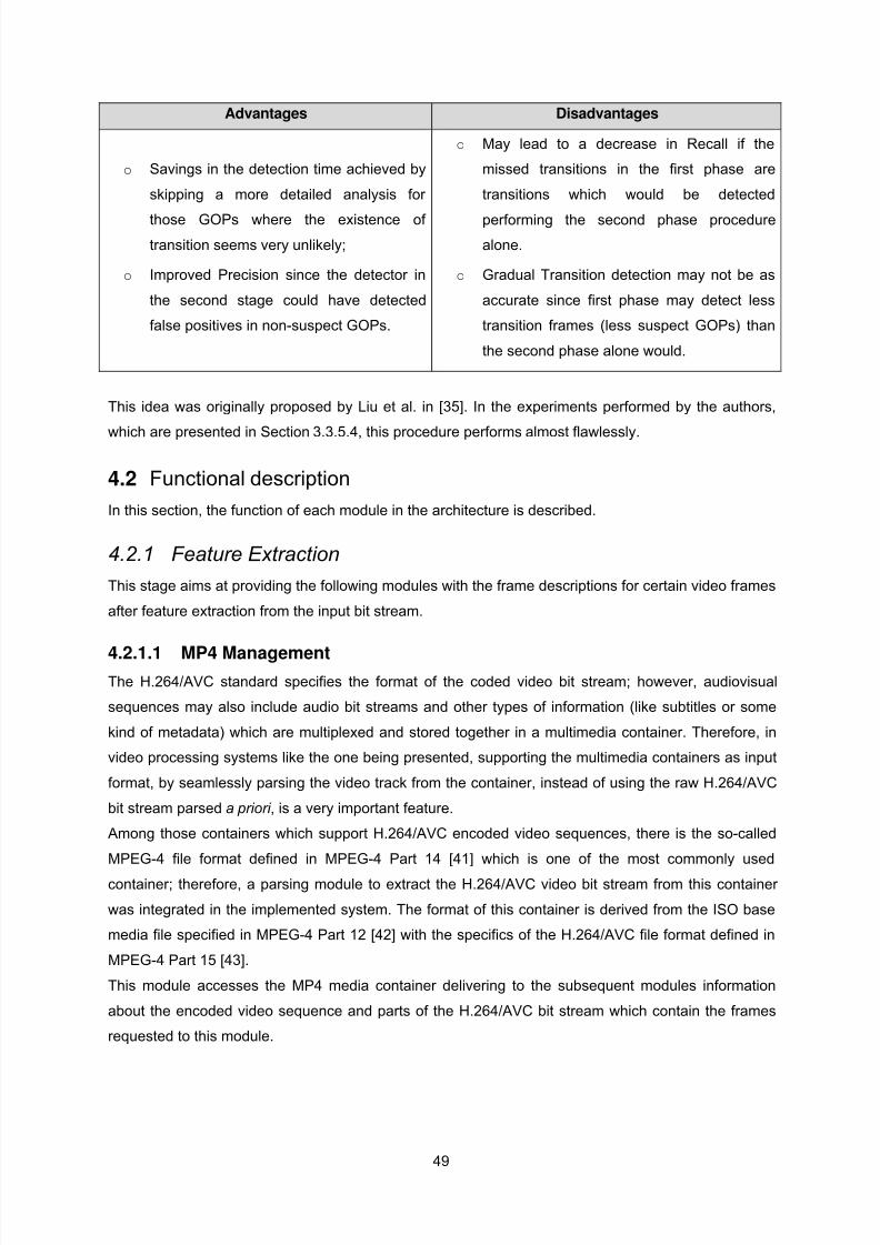
8/14/2019 H.264 Compressed Shot Detection
http://slidepdf.com/reader/full/h264-compressed-shot-detection 69/128
Advantages Disadvantages
o Savings in the detection time achieved by
skipping a more detailed analysis for
those GOPs where the existence of
transition seems very unlikely;
o Improved Precision since the detector in
the second stage could have detected
false positives in non-suspect GOPs.
o May lead to a decrease in Recall if the
missed transitions in the first phase are
transitions which would be detected
performing the second phase procedure
alone.
o Gradual Transition detection may not be as
accurate since first phase may detect less
transition frames (less suspect GOPs) than
the second phase alone would.
This idea was originally proposed by Liu et al. in [35]. In the experiments performed by the authors,
which are presented in Section 3.3.5.4, this procedure performs almost flawlessly.
4.2 Functional description
In this section, the function of each module in the architecture is described.
4.2.1 Feature Extraction
This stage aims at providing the following modules with the frame descriptions for certain video frames
after feature extraction from the input bit stream.
4.2.1.1 MP4 ManagementThe H.264/AVC standard specifies the format of the coded video bit stream; however, audiovisual
sequences may also include audio bit streams and other types of information (like subtitles or some
kind of metadata) which are multiplexed and stored together in a multimedia container. Therefore, in
video processing systems like the one being presented, supporting the multimedia containers as input
format, by seamlessly parsing the video track from the container, instead of using the raw H.264/AVC
bit stream parsed a priori , is a very important feature.
Among those containers which support H.264/AVC encoded video sequences, there is the so-called
MPEG-4 file format defined in MPEG-4 Part 14 [41] which is one of the most commonly used
container; therefore, a parsing module to extract the H.264/AVC video bit stream from this container
was integrated in the implemented system. The format of this container is derived from the ISO base
media file specified in MPEG-4 Part 12 [42] with the specifics of the H.264/AVC file format defined in
MPEG-4 Part 15 [43].
This module accesses the MP4 media container delivering to the subsequent modules information
about the encoded video sequence and parts of the H.264/AVC bit stream which contain the frames
requested to this module.
49
8/14/2019 H.264 Compressed Shot Detection
http://slidepdf.com/reader/full/h264-compressed-shot-detection 70/128
4.2.1.2 Low-level Features Extraction
As explained in Chapter 3, there are several features which can be used for shot transition detection.
However, to meet the requirements defined for the algorithms to be implemented, namely, to operate
in the H.264/AVC compressed domain, the list of available features is shortened being constrained to
encoding information like the prediction modes used by the encoder.
4.2.1.3 Frame Descriptions Generation
In this first stage, the low-level features received from the previous modules are analyzed and the
corresponding frame descriptions are generated and delivered to the next module in the processing
chain.
There are two of such modules in this system: one under the suspect GOP detection phase and
another under the transition detection phase. The output descriptions may vary according to the type
of frame being analyzed and the chosen algorithm. Among the descriptors used are, for example,
ratios, like the ratio of intra predicted macroblocks, or histograms, like the distribution of the used
macroblock types and inter or intra prediction modes.
Since a hierarchical transition detection solution with two phases is proposed, the frame descriptions
generation module has different functions in the context of these two phases, notably:
o 1st phase: Suspect GOP detection – In this module, only intra frames will be considered;
therefore, the output descriptors will be based on intra prediction features, like luminance intra
prediction modes, as introduced in [35], chrominance intra prediction modes and luminance
partition sizes, as described in [16].
o 2nd phase: Transition detection – The differences between this module and the
corresponding one under the Suspect GOP detection are related to the type of frames
processed; in the previous module, only intra frames were considered whereas in this module P
and B frames must also be considered.
4.2.2 Similarity/Difference Score Computation
This module aims at using the frame descriptions received to generate scores which estimate the
continuity or discontinuity in the video content over the analyzed frames. These scores are then
outputted to the subsequent modules.
Since the descriptions output by the module above can vary, depending on the chosen algorithm and
the frame types, various methods will be used by this module to compare frames. For each computed
value, this module may take in consideration descriptors for one frame, for a pair of frames
(consecutive or not) or for several frames. As in the previous module, this one also is duplicated:
o 1st phase: Suspect GOP detection – In this module a difference is computed by comparing
the descriptors from the first frame of the current GOP against those from the first frame of the
next GOP. The purpose of this computed difference is to estimate the difference between both
frames.
o 2nd phase: Transition detection – The methods used in this module may evaluate the
discontinuity by detecting gaps in the prediction chain, using prediction direction descriptors, by
50

8/14/2019 H.264 Compressed Shot Detection
http://slidepdf.com/reader/full/h264-compressed-shot-detection 71/128
focusing on the difference between partitions map, using mainly macroblock types, or by mixing
the two approaches. For each computed value, this module may take into account descriptors
from one frame, from a pair of frames (consecutive or not) or from several frames in the suspect
GOPs.
4.2.3 Decision
This module aims at analyzing the scores obtained in the previous module to decide if whether they
seem to reflect a shot change or not. There are two decision modules in the architecture:
o 1st phase: Suspect GOP detection – This is called GOP Classification and aims at classifying
GOPs as suspect or not of having an abrupt or gradual transition, based on the evaluation of
the difference scores obtained earlier.
o 2nd phase: Transition detection – This module groups the frames where some kind of
discontinuity is found and performs some post-processing to convert those positives to a set of
transitions which will be the final output of this stage.
4.2.4 Detection Evaluation
This module is used to evaluate the performance of both phases in the transition detection. For that
purpose an XML description of the shot structure of the movie under analysis is required.
4.2.5 Shot Structure Description
To ensure the interoperability of this system with other systems which need the description of shot
transitions in a video, the shot structure description of the analyzed video, as detected by the previousmodules, is saved into an XML file.
In the following chapter, the algorithms used to implement each module will be described in detail.
51

8/14/2019 H.264 Compressed Shot Detection
http://slidepdf.com/reader/full/h264-compressed-shot-detection 72/128

8/14/2019 H.264 Compressed Shot Detection
http://slidepdf.com/reader/full/h264-compressed-shot-detection 73/128
CHAPTE
Algorithms: Processing
R 5
fore, the various
algorithms implemented for each of these phases will be described in the following.
s are
y independently choosing one algorithm for each module from those
presented in the following.
ints (RAP) frames. Each solution for this sub-module can be characterized
tions generated may be based on the following features:
In this chapter, the algorithms designed and developed for processing the video data in order to detect
shot transitions will be described. This is a high-level description and will cover the modules in the
architecture which are directly related to the shot detection. Several algorithms were implemented for
shot detection, both in the suspect GOP detection and in the transition detection phases with the
purpose of comparing the performance of several different approaches; there
5.1 First Phase: Suspect GOP Detection
As previously referred in Chapter 3, this Thesis adopted for the proposed transition detection system a
two-layer architecture, as initially introduced in [35] and briefly explained in Section 3.3.4; while this
section will present the algorithms for the first phase – suspect GOP detection – the next section will
present the algorithms for the second phase – transition detection phase. The output of the suspect
GOP detection phase is a list of GOPs which most likely contain GOP transitions and thu
analyzed with more detail in the second phase for a more precise localization of the transitions.
As shown in Chapter 4 (Figure 4.1), the suspect GOP detection phase considers three main modules:
frame description generation, GOP difference score computation and GOP classification. In the next
sub-sections, the algorithms used in each module will be presented. Various suspect GOP detection
phase algorithms result b
5.1.1 Frame Description Generation
This sub-module aims at generating descriptions for each frame marking the beginning of a GOP; this
means Random Access Po
by two major components:
o Features used – The frame descrip
53

8/14/2019 H.264 Compressed Shot Detection
http://slidepdf.com/reader/full/h264-compressed-shot-detection 74/128
Luminance Prediction Modes;
Luminance and Chrominance Prediction Modes;
k a description is generated;
ot divided but it is rather analyzed as a whole and only one
nd frame granularity.
imilar intra prediction
encode more detailed areas whereas bigger partitions are used to encode smoother
usually depends on the content and textures being encoded
ution
ver a frame was therefore proposed. Accordingly:
s (9 representing the 4 x 4 intra prediction modes and 4 for the 16 x 16 intra prediction
normalized dividing the value of each bin for the number of 4 x 4 blocks which
displayed which will be used to
(a) (b)
Luminance Partition Types.
o Spatial granularity – The same descriptions may be made at two granularity levels:
Block – Each frame is divided into blocks and for each bloc
these block descriptions together form the frame description.
Frame – The frame is n
description is generated;
The original algorithm in [35] uses the luminance prediction modes as features a
5.1.1.1 Features Algorithm 1: Luminance Prediction Modes
In [35], the authors claim that the intra prediction modes used to encode one frame reflect the visual
content being encoded and, therefore, similar content should be encoded using smodes. Each intra prediction mode is basically characterized by two dimensions:
o Partition sizes – This usually reflects the granularity of the visual content; smaller partitions are
used to
areas.
o Intra prediction direction – This
rather than the granularity.
Thus, the algorithm proposed in [35] requires the creation of the histogram describing the distrib
of the luminance intra prediction modes used oo Each frame is divided into 4 x 4 blocks;
o Each block is classified according to the intra luminance prediction mode used into 13
categorie
modes)
o The histogram is
form the frame.
In Figure 5.1, three sample frames from a high definition video are
exemplify some of the concepts in this and in the following sections.
54

8/14/2019 H.264 Compressed Shot Detection
http://slidepdf.com/reader/full/h264-compressed-shot-detection 75/128
(c)
Figure 5.1 – Three sample frames extracted from the “BBC Motion Gallery presents CCTV” videosequence downloaded from the Apple HD Gallery [44]. a) Frame 309, b) Frame 5078, c) Frame 5383.
In Figure 5.2, the luminance intra prediction histograms for the frames in Figure 5.1 are depicted. By
analyzing the visual content in the frames and the corresponding histograms, it is possible to verify the
assumptions mentioned earlier, notably:
o A comparison between the description a) with either the description b) or c) seems to confirm
the idea that frames which contain more detail use mainly smaller partition whereas frames with
a more smooth content use bigger partitions.
o By comparing descriptions b) and c), it is possible to observe that the differences in the visual
content may yield also differences in the intra prediction direction even if the partition sizes used
are similar.
(a) (b)
55

8/14/2019 H.264 Compressed Shot Detection
http://slidepdf.com/reader/full/h264-compressed-shot-detection 76/128
(c)
Figure 5.2 – Updated frame descriptions corresponding to the H.264/AVC High profile coding for theframes in Figure 5.1.
However, this algorithm does not take into account some other intra prediction mode possibilities. In
fact, in addition to the previously introduced luminance intra prediction modes, there are also modes
based on 8 x 8 partitions, which were added later to the standard; these modes are only available in
the H.264/AVC High profile, and the PCM encoding mode, although this last is rarely used. Despite
these modes being less common, they should be added to the histogram; therefore, a modification in
the original algorithm is needed extending the histogram descriptor from 13 to 23 bins
An example of such descriptions, still for the frames presented in Figure 5.1, is displayed in Figure 5.3;
by analyzing these descriptions, it is possible to observe that, despite the introduced modification, the
same assumptions made for the original algorithm are still true and thus the algorithm still works as
intended.
(a) (b)
56

8/14/2019 H.264 Compressed Shot Detection
http://slidepdf.com/reader/full/h264-compressed-shot-detection 77/128
(c)
Figure 5.3 – Updated frame descriptions corresponding to the H.264/AVC High profile coding for theframes in Figure 5.1.
5.1.1.2 Features Algorithm 2: Luminance and Chrominance Prediction Modes
Based on the same assumption described in the previous section, the chrominance prediction modes
may also reflect the encoded content and, therefore, may be a useful addition to the generated
descriptions. With this purpose in mind, 4 additional bins reflecting each of the intra chrominance
prediction modes are added, by the author of this Thesis, to the 23 previously introduced, each
representing a chrominance prediction mode.
Some examples of the novel histograms, corresponding to the frames in Figure 5.1, are depicted in
Figure 5.4. After inspection of these frame descriptions, the relation between the chrominance
prediction modes used and the encoded content is evident and, therefore, it is reasonable to also
consider these modes for the purpose of shot detection, since there might be frames belonging to
different shots which may be encoded using similar luminance intra prediction modes but different
intra chrominance prediction modes.
(a) (b)
57

8/14/2019 H.264 Compressed Shot Detection
http://slidepdf.com/reader/full/h264-compressed-shot-detection 78/128
(c)
Figure 5.4 – Frame descriptions corresponding to the H.264/AVC High profile coding for the frames inFigure 5.1 considering also the intra chrominance prediction modes.
5.1.1.3 Features Algorithm 3: Luminance Partition Types
Another method for description extraction for intra frames is presented in [16]. In this paper, luminance
partition types are used as features when processing intra frames, generating a histogram composed
of 3 bins, each representing a partition type relative frequency (16 x 16, 8 x 8 and 4 x 4) over the
block. By observation of Figure 5.3, it can be seen that partition sizes can trigger transitions; however,
this does not seem as accurate as considering prediction modes also.
5.1.1.4 Granularity Algorithm 1: Frame Granularity
Using this approach, the feature extraction will be processed generating a histogram which
corresponds to the entire frame. This mode may not be as sensitive as the block based alternative but
may be more invariant.
5.1.1.5 Granularity Algorithm 2: Block Granularity
Two block based approaches were implemented for this module:
o Window – The frame description is composed of block descriptions for each window of N x M
macroblocks around each macroblock (N and M being odd numbers). This approach is
presented in [16] and has the advantage of providing the generated descriptions with some
spatial information. This can be useful since there are frames which may belong to different
shots and may have a similar global content; however, by analyzing the frames in terms of local
spatial properties, the spatial differences they may have are considered. However, there is a
disadvantage in using this windowed approach: it increases the computation complexity of this
operation since the same macroblock is considered more than once in the computations.
o Non-overlapping blocks – In this case, the frame is partitioned into non-overlapping blocks of
size N x M macroblocks; if the height or width of the frame cannot be divided by the block
58

8/14/2019 H.264 Compressed Shot Detection
http://slidepdf.com/reader/full/h264-compressed-shot-detection 79/128
dimension, the remaining macroblocks at the edges are discarded. Comparing to the window
approach, this is faster since the blocks are not overlapping.
5.1.2 GOP Difference Score Computation
As addressed in the previous section, differences in the visual content may generate differences in thestatistical distribution of the histograms which compose the descriptions. There are several ways of
measuring such differences. However, in the developed system, the two metrics implemented are:
o Sum of absolute differences – The sum of absolute differences was the metric originally
proposed in [35]; in the current implementation, the only modification was the normalization of
the metric leading to (15).
(15)
o Variant of Pearson’s homogeneity test – A variant of the Pearson’s homogeneity test was
implemented; this metric (16) was the solution which better performed in a test carried out in
[20] for luminance histograms; here, it is normalized and proposed to be used for intra
prediction modes histograms instead.
(16)
To generate the difference score between two frames for the features defined in the previous section,
a metric has to be chosen to compare the block descriptions from the corresponding blocks in those
frames (frame descriptions taken at frame granularity are considered as block descriptions with only
one block); afterwards, the scores obtained for the blocks are summed to generate the frame score
difference. In this sub-module, a difference score is generated for each GOP which is computed by
comparing the first frame of the current GOP (f a) with the first frame of the next one ( f b) as in (17). In
Figure 5.5, some examples of such difference scores are depicted.
(17)
5.1.3 GOP Classification
This last module of the suspect GOP detection phase aims at classifying e GOP in the H.264/AVC
coded stream as suspect or not in terms of shot transition. As referred in Section 3.1, there are several
methods to achieve this goal; in the developed system, two algorithms were implemented to classify
each GOP, notably:
o Fixed threshold – Each score is compared to a fixed threshold (Tf ) heuristically set before the
analysis as in (18); this is the procedure used in [35].
59

8/14/2019 H.264 Compressed Shot Detection
http://slidepdf.com/reader/full/h264-compressed-shot-detection 80/128
(18)
(a) (b)
Figure 5.5 – GOP Difference Scores for the video sequences introduced in Figure 5.1 using the intraluminance prediction modes descriptor with frame granularity and (a) Sum of Absolute Differences and
(b) Variant of Pearson’s Test
o Adaptive threshold – An adaptive threshold is computed for each frame taking into
consideration the difference scores from surrounding GOPs which form a window of difference
scores. There are some alternatives regarding the difference scores to consider in this window:
it has N samples which may be centered on the current GOP or contain only values obtained
from previous GOPs and the value of the current GOP may or not be discarded (depending on
the chosen option). There are two basic approaches implemented:
Average-based threshold - this threshold is computed using the expressions (19), (20) and
(21), where a and b are heuristically set coefficients and µ (average) and σ (standard
deviation) are calculated using the window of difference scores. The minimum and
maximum values in (20) and (21) are used to exclude extreme values which may happen,
for instance, at the beginning or at the end of a video sequence where the window might
not be completed. After this calculation, the similarity score is compared with the computed
adaptive threshold.
(19)
(20)
(21)
Median-based threshold - this threshold is computed using the expressions (22), (23) and
(24), where a and b are heuristically set coefficients and Median is calculated using the
window of difference scores. The minimum and maximum values in (20) and (21) are used
to exclude extreme values which may happen, for instance, at the beginning or at the end
of a video sequence where the window might not be completed. After this calculation, the
similarity score is compared with the computed adaptive threshold.
60
8/14/2019 H.264 Compressed Shot Detection
http://slidepdf.com/reader/full/h264-compressed-shot-detection 81/128
(22)
(23)
(24)
Those GOPs for which the difference score value is above the threshold T a, as in (25), are considered
suspect GOPs and are added to the set of suspect GOPs which will, at the end of this procedure, be
provided to the next modules in the system, this means, to the second phase of transition detection.
The last GOP of the video sequence is always considered suspect.
(25)
5.2 Second Phase: Transition Detection
This phase targets the detection of the frames in which a transition occurs for the GOPs which have
previously been considered as suspect. For this phase, four algorithms were implemented:
o Algorithm 1 – The shot detection algorithm described in Section 3.3.3 and proposed in [34] and
in [33].
o Algorithm 2 – A shot detection algorithm inspired by Algorithm 1 but with some modifications
proposed by the author of this Thesis to improve its performance.
o Algorithm 3 – A shot detection algorithm based on the system proposed in [16] with some
modifications made by the author of this Thesis.
o Algorithm 4 - A shot detection algorithm using hierarchical detection based on the system
proposed in [16] with some modifications made by the author of this Thesis.
These four algorithms will be described in detail in the next sections. This description aims at the
functioning of the algorithm using constant GOP structures of N=15 and M=3, which will be used at
evaluation. Despite that fact, the algorithms can be easily extended to support other GOP structures.
Remind that, according to the architecture presented in Chapter 3, each transition detection algorithms
considers three sub-modules: frame description generation, similarity score computation and decision.
5.2.1 Algorithm 1
This first algorithm here described has been proposed in [34] and [33] and was briefly described inSection 3.3.3. As it was explained, the key idea of this algorithm is to detect transitions by analyzing
changes in the partition sizes and partition types and the usage of intra prediction modes in P and B
frames. This algorithm was tested by its authors only using videos encoded with the Baseline Profile,
which does not allow B frames, which means it was never tested when for B frames.
In this section, a detailed description of the algorithm used in each module will be provided.
5.2.1.1 Frame Description Generation
In this algorithm, only B and P frames are evaluated; each of these frames is described by two
different descriptors:
61

8/14/2019 H.264 Compressed Shot Detection
http://slidepdf.com/reader/full/h264-compressed-shot-detection 82/128
o Partition histogram (PH) – This descriptor accounts for the inter partition sizes and types used
in each frame.
o Intra block ratio (IBR) – This descriptor contains the ratio of intra coded macroblocks in the
current frame.
Partition Histogram
For the generation of this type of description, each frame is split into each 4 x 4 blocks and each block
is grouped according to its prediction type (P, if forward prediction, B, if backwards, interpolated or
direct prediction, or skipped prediction) and size of the corresponding prediction partition into 15 bins:
P16 x 16
, P16x8
, P8x16
, P8 x 8
, P8x4
, P4x8
, P4 x 4
, B16 x 16
, B16x8
, B8x16
, B8 x 8
, B8x4
, B4x8
, B4 x 4
and S16 x 16
.
Intra prediction partitions are not considered because the authors argue it would produce too many
false positives since these prediction modes may be used also due to fast motion; instead the usage
of such prediction type is indirectly considered due to effect its rises and falls produce in the usage of
the considered partition types.
Intra Block Ratio
As it is done for generating the PH descriptor, in this case the frame is also split into 4 x 4 blocks;
afterwards, the ratio of those blocks belonging to intra prediction partitions is computed. As the intra
blocks are used for new content, high usages of intra prediction modes may appear when a shot
transition is taking place; however, this may also happen when encoding frames with fast motion.
These descriptors are exemplified in Figure 5.6. In this figure, it is possible to observe the differences
in the PH description and a significant increase in the IBR description value in consecutive frames
which belong to different shots.
Figure 5.6 – Two frame descriptions taken from two consecutive P frames belonging to different shots; ineach figure, it is possible to observe the PH description at the 8 leftmost bins and the IBR description at
the rightmost bin.
5.2.1.2 Difference Score Computation
In this transition detection phase, this score accounts for the discontinuity in the visual content at the
frame being analyzed; higher values mean a higher probability of a shot change taking place and vice-
versa. With this purpose, two scores are implemented for this algorithm, for each frame, notably:
62

8/14/2019 H.264 Compressed Shot Detection
http://slidepdf.com/reader/full/h264-compressed-shot-detection 83/128
o Partition histogram difference (PHD) – This metric evaluates the differences between frames
by comparing the corresponding PH descriptions; the descriptions of the current and previous
frames are compared according to (26), based on the sum of absolute differences, or to (27),
based on the sum of non-absolute differences. According to the experiments realized by the
authors who proposed this algorithm, the later performs better yielding less false positives whencompared to the first [33], since there are some cases where partitioning changes, not due to
real content change, but due to compression efficiency decisions of the encoder, e.g., if an
encoder starts to use Skipped macroblocks instead of predicted macroblocks. However, this
seems contradictory with the partition change detection since the changes using non-absolute
differences will be only due to intra ratio change (rises and falls) and not due to partition
changes.
f 1N
, N
(26)
f 1N , N
(27)
o Intra block ratio (IBR) – Regards the direct usage of the IBR description for the current frame;
for each frame, this is equal to the ratio of intra coded macroblocks in that frame.
5.2.1.3 Decision
In this last sub-module of the second phase, the similarity scores previously obtained are analyzed. As
it was previously referred, high difference scores stand for a high degree of dissimilarity in the frames
analyzed; therefore, by detecting those frames which correspond to high difference scores transitions
may be detected.
In the original algorithm [34] [33], Schöffmann et al. state that a frame should be considered as a
candidate for an abrupt transition if its PHD is equal (28) or above a predefined fixed threshold (TPHD)
or if its IBR is equal or above ano e efi e ) (29).ther fix d pred ned thr shold (TIBR
f f
(28)
f f (29)
These candidates are added to the respective PDH or IBR candidate set which will be provided to a
post-processing procedure to transform this candidate set into a definitive transition set. This post-
processing is a three step procedure including:
o Gradual transition detection – This step is meant to group frame candidates that seem to
belong to gradual transitions. In this step, frames in the candidate set which are less than Δ
frames apart from each other as in (30) are grouped; this is to tolerate “detection holes” which
span over a maximum of Δ frames. If this group obeys to the size constraints as in (31), then it
is considered a valid group, added to a gradual transition candidate set and the corresponding
original abrupt candidates are removed from the set, otherwise the group is discarded and the
63

8/14/2019 H.264 Compressed Shot Detection
http://slidepdf.com/reader/full/h264-compressed-shot-detection 84/128
original abrupt candidates remain in the abrupt candidate set. There are two sets of these three
parameters: one for the oth r r the RPHD and the e fo IB .
… , 1
|| 1
∆ (30)
(31)
o Consecutive cut removal – This rule (32) excludes from the candidate set abrupt candidates
which are too close from each other assuming that shots have to be more than μ frames length.
This comparison is checked starting in the last cut candidate, which is compared to the previous
cut candidate a d xcl it s and ndidate is reached.n e uded if i too close, performed until the first ca
µ excludedfromcandidateset (32)
o IBR/PHD combination – This last step aims at combining the IBR and PHD approaches in
order to create the detection set. In their experiments, Schöffmann et al. found that PHD alone
works fine for cut detection; however, it lacks in gradual detection. On the other hand, IBR
works better for gradual detection since it yields many false positives in cut detection.
Therefore, after the previous post-processing steps, the PHD candidate cuts are added to the
detected transition set and only gradual transitions are added to that set among the IBR
candidates.
5.2.2 Algorithm 2
As mentioned before, Algorithm 1 was only tested by its authors using videos encoded with the
Baseline Profile; in fact, the description of the algorithm’s operation when using sequences encodedwith other profiles provided in both [34] and [33] seems to lack functionality. Therefore, a second
algorithm – Algorithm 2 - was designed by the author of this Thesis, still inspired by the ideas
underpinning Algorithm 1 with the main purpose of improving its performance.
5.2.2.1 Frame Description Generation
Algorithm 2 uses the same type of descriptors as proposed for Algorithm 1. Comparing the descriptors
in the two algorithms, the significant differences are in the PH descriptor; these modifications aim at
enhancing the previous algorithm for B frames. With this purpose in mind, two major modifications in
the definition of the descriptors are proposed:
o Modification 1: Partition classification - The first major modification proposed is to classify
the partitions based on their size and prediction direction; since the objective of this algorithm is
to use the partition approach adopted by Algorithm 1, the size still plays a major role in these
descriptors. Therefore, the B prediction type is split into interpolated (I) and backward (B)
prediction types with the skipped partitions being considered as forward partitions (either P16 x 16
or P8 x 8
depending in the partition size); this extends the histogram to 21 bins (P16 x 16
, P16x8
,
P8x16
, P8 x 8
, P8x4
, P4x8
, P4 x 4
, B16 x 16
, B16x8
, B8x16
, B8 x 8
, B8x4
, B4x8
, B4 x 4
, I16 x 16
, I16x8
, I8x16
, I8 x 8
, I8x4
,
I4x8
and I4 x 4
). In this way, the prediction direction is meant to be provided with more importance
than it had in the original algorithm which is only based on the prediction types.
64

8/14/2019 H.264 Compressed Shot Detection
http://slidepdf.com/reader/full/h264-compressed-shot-detection 85/128
o Modification 2: Direct mode classification - Direct mode predicted partitions should also be
classified according to its prediction direction instead of simply classifying all as the same as in
Algorithm 1. As referred in Chapter 1, there are two types of direct prediction modes:
Temporal direct – Partitions encoded in using this mode always use interpolated
prediction and, therefore, are classified as I16 x 16
or I8 x 8
according to its size.
Spatial direct – Partitions encoded in this mode can have backward, forward or
interpolated prediction. The prediction direction of partitions encoded using this mode is not
parsed from the bit stream; instead, the reference indexes and motion vectors used are
inferred in later phases of the decoding process. These phases are not performed in the
implemented low-level feature extraction module but a similar method, which will be
described in the next sub-section, was designed and implemented to infer the prediction
direction of a spatial direct partition. Therefore, these partitions can be considered as P16 x
16, P
8 x 8, B
16 x 16, B
8 x 8, I
16 x 16or I
8 x 8according to its prediction direction and size.
Inference of the prediction direction in direct spatial mode
In the direct mode, the encoder does not include motion information in the bit stream; instead, the
motion information is inferred by the decoder using the motion information from adjacent blocks. More
precisely, as depicted in Figure 5.7, to infer the motion information of a direct coded block in
macroblock E, the decoder uses motion information from blocks A, B, C and D, this last only replaces
C whenever C is not available. The process defined in the standard to do this is the following:
o For each reference list, consider the minimum reference index, associated to that list, among
those used in A, B and C. If all neighbors are encoded in intra mode or if none uses the current
list for inter prediction, this step is considered unsuccessful.
If the preceding process was successful, if the associated reference index is zero and if the
motion vector from the collocated block in the first list_1 reference is considered stationary,
the motion vector for the current list is set to zero.
Else, if the reference index inferring was successful tor the current list, the associated
motion vector is inferred considering the motion vectors neighbor blocks which use the
inferred reference index for that list.
o If neither reference index is successfully inferred, both reference indexes set to zero and both
motion vectors are also set to zero.
Figure 5.7 – Motion vector prediction for direct blocks in E is performed by analyzing motion informationfrom blocks A, B and C or D.
65

8/14/2019 H.264 Compressed Shot Detection
http://slidepdf.com/reader/full/h264-compressed-shot-detection 86/128
In this work, however, this is not necessary, since motion vectors and reference indexes are not used,
due to the work requirements. Therefore, an alternative method is proposed by the author of this
Thesis to infer the prediction direction which is less complex than standard motion inferring:
o The same blocks, A, B and C or D, are taken in consideration;
o If any uses both reference lists or if there are both blocks using list0 and blocks using list1, then
interpolated prediction is assumed for direct mode in macroblock E;
o Else, if all blocks are encoded in inter prediction mode using list list0 , forward prediction is
assumed;
o Else, if all blocks are encoded in inter prediction mode using list1, backward prediction is
assumed;
o Else, if all use intra prediction, interpolated prediction is assumed.
5.2.2.2 Similarity Score CalculationThe algorithms used in this module were also changed regarding the solutions from Algorithm 1; two
difference scores are proposed:
o IBR – The same as in the original algorithm with no modifications;
o PHD – In this score, some modifications are proposed to enhance its operation. They target the
better functioning of the original algorithm when B frames are involved since, as previously
outlined, the original algorithm does not cope well with B frames. Besides the slight change
which the new extended descriptions would obviously impose, the assumption that frames
should be compared equally disregarding their type or relative position does not seem accurate.
Instead, before computing the differences as depicted in (26) or (27), the frame types and
relative positions are considered as follows in order to make those frames comparable:
B Frame vs. P Frame – When the previous frame is a B frame and the current is a P
frame, the descriptions in B are modified for the purpose of this comparison by considering
all interpolated and backwards predicted partitions as forward prediction. This is done so
there are less false positives; in fact, if a B frame followed by a P frame uses mainly
interpolated or backwards prediction a shot transition should not be detected due to the
decrease in the usage of those prediction directions.
P Frame vs. B Frame – When the previous frame is a P frame and the current is a B
frame, the B frame descriptions are changed by summing the values which correspond to
the interpolated predicted bins with the corresponding bin in the forward prediction bin, for
the same reason as in the previous case, and by considering backwards predicted blocks
as intra blocks, since this is a what was expected to happen if there was a P frame in that
place.
I Frame vs. B Frame – Contrary to what happens in baseline profile, using the main profile
a shot may be detected only considering the prediction direction of the B frames that
follows an I frame. For that matter, a score in this comparison will be calculated considering
66
8/14/2019 H.264 Compressed Shot Detection
http://slidepdf.com/reader/full/h264-compressed-shot-detection 87/128
the macroblocks in the I frame as P macroblocks and considering the B frame as in the last
comparison (P frame vs B frame).
Same Type (P or B) – When comparing frames of the same type, no change in the
descriptions is needed.
In these scores, the regular intra frame processing is also performed in a similar fashion as in the
original algorithm (Algorithm 1).
5.2.2.3 Decision
The algorithm used to identify the transitions based on the difference scores is similar to that in
Algorithm 1. As in the previous algorithm two candidate sets are created using the same thresholding
procedure (33) and (34).
f f
(33)
f f (34)
Afterwards a similar post-processing is employed to transform the candidate sets into a transition set:
o Gradual transition detection – This step is meant to group IBR frame candidates that seem to
belong to gradual transitions and is equal to that presented for the original algorithm (30) and
(31).
o Consecutive cut removal – This excludes from the candidate set abrupt candidates which are
too close from each other and is equal to that presented in (32).
o Consecutive gradual transition joining – This aims at joining gradual transitions which are
overlapped or too close from each other, in which case would yield a very short shot between
the two.
o Cut/Gradual transition set combination – Cuts from PHD candidate set and gradual
transitions from the IBR candidate set are added to the transition set.
5.2.3 Algorithm 3:
This third algorithm was defined mainly to compare the partition approach, outlined in the previous
algorithms, with a gap-in-prediction chain approach which was partially adopted from [16]. This
algorithm compares successive frames to detect both gradual and abrupt transitions. This algorithm
can be divided in three procedures:
o Abrupt transition detection relying on temporal dependences (Inter procedure) – This
uses information from macroblocks belonging to inter frames and can be compared to the
previous abrupt detection approaches.
o Abrupt transition detection relying on spatial information (Intra procedure) – This uses
information from both inter and intra coded frames and is meant to complement to the Inter
procedure.
o Gradual trandition detection (Grad procedure) – This is meant to detect gradual transitions.
67

8/14/2019 H.264 Compressed Shot Detection
http://slidepdf.com/reader/full/h264-compressed-shot-detection 88/128
5.2.3.1 Frame Description Generation
Two frame descriptors were adopted and implemented from [16] for this Algorithm 3, notably:
o Prediction direction – This is used to describe the temporal dependencies of the frame under
analysis; with this purpose, each frame is partitioned into 8 x 8 blocks and each is classified
according to the prediction direction used: intra, forward, backwards or interpolated. This gives
rise to a 4 bin histogram which is normalized by diving each bin by the number of 8 x 8 blocks
which form the frame. As for the previous algorithm, the inference procedure for prediction
direction in direct coded partitions described in Section 5.2.2.1 was implemented to classify
those partitions. This is related with the Inter procedure.
o Intra prediction map – This is used to describe the spatial characteristics of a certain frame. It
is constructed for two frames in a GOP: the first and the last, and contains the intra prediction
encoding information (as it is done in the suspect GOP detection phase); Each prediction map
starts being constructed at the beginning of the GOP (I frame) and advances trough its Pframes until the frame for which the map is being constructed is reached; meanwhile, every time
an intra coded macroblock is found in those frames, the corresponding macroblock prediction
information in the prediction map is updated. After updating this prediction map with the current
frame, intra frame descriptors are generated for that prediction map using the same algorithms
presented in Section 5.1.1. This is related with the Intra procedure.
In the original algorithm in [16], another descriptor is proposed: the motion intensity for the foreground
and background areas of the picture which is used in the gradual transition detection. However,
motion extraction from the H.264/AVC bit stream is not a straightforward procedure since the motion
vectors are not directly available from the bit stream; instead, only the differential motion vectors are
available and can be parsed from the bit stream. To compute the motion vectors, a motion vector
prediction has to be inferred from neighbor partitions, which is only done in late stages of the decoding
process.
5.2.3.2 Similarity Scores Computation
In this algorithm, four scores are calculated with the purpose to express the continuity and
discontinuity between frames:
o Sum of intra and forward predicted block ratios for previous frame (s1 ) - This expresses
continuity in the previous frame related to the video content before it and it is calculated for
every inter frame. This is related with the Inter procedure.
o Sum of intra and backward predicted block ratios for current frame (s2 ) - This expresses
discontinuity in the video content between the previous and current frame and it is calculated for
every inter frame. This is related with the Inter procedure.
o Intra block ratio (IBR) – This is the IBR for the current frame; this is only calculated in P frames
and is related with the Grad procedure.
o Intra frame difference (Dintra ) – Unlike the previous scores, this is not computed for all frames;
instead, it is used to calculate differences between an intra prediction map belonging to a P
68
8/14/2019 H.264 Compressed Shot Detection
http://slidepdf.com/reader/full/h264-compressed-shot-detection 89/128
frame, that at the end of each GOP, and an intra frame, that at the beginning of the succeeding
GOP; to calculate such score, the algorithm described in Section 5.1.2 is used. This is related
with the Intra procedure.
5.2.3.3 Decision
The decision process for transition detection in this algorithm is based on the similarity scores defined
earlier as in [16]:
o Abrupt Transitions - If both s1 and s2 are above a predefined fixed threshold (T Inter ), then a gap
in the prediction chain is detected. The outcome of this comparison may be:
If the current frame is neither an I nor an IDR frame, a transition is detected.
If the current frame is an IDR or an I frame, the Dintra score must be considered; this score
is computed between the current frame and the intra prediction map of the previous frame.
An adaptive threshold (T intra) is also computed, similar to that presented in Section 5.1.3; a
window of N previous intra frame difference values is considered to calculate the terms µ
and σ in (19); the rest of the terms are defined heuristically. If the obtained score is above
the computed t r h ab r n ch es old, an rupt t a sition is dete ted.
f & f f D
(35)
f f (36)
o Gradual Transitions - This is focused on the analysis of the IBR scores of P frames. In this
case, another adaptive threshold is computed based on the expressions (19), (20) and (21) by
analyzing a window of N previous IBR scores in P frames. If the current IBR score is above the
threshold computed for the corresponding frame, it is considered as a candidate for a gradual
transition; afterwards, a post-p c sta 2 is executed.ro essing ge as for Algorithm
IBRf f (37)
At the end, the detected transitions, both the gradual and abruptm are added to the transition set.
5.2.4 Algorithm 4
This third algorithm was inspired by the hierarchical approach in [16]. It is meant to improve the
algorithm 3 in two ways:
o A different method for detecting abrupt transitions comparing P frames;
o The introduction of hierarchy in the detection to avoid false positives. By observation of the
results of the previous algorithms in the Main profile, it can be noted that B frames sometimes
trigger abrupt transitions which do not occur and could be avoided by analyzing the P/I
reference frames that surround the B frames. Therefore, a two layer algorithm is suggested
where one layer is composed by the non-reference B frames.
This algorithm is designed to detect both gradual and abrupt transitions.
69

8/14/2019 H.264 Compressed Shot Detection
http://slidepdf.com/reader/full/h264-compressed-shot-detection 90/128
5.2.4.1 Frame Description Generation
The same frame descriptors used in Algorithm 3 are used without any kind of modification.
5.2.4.2 Similarity Scores Computation
In this algorithm, the same four scores, as in algorithm 3, are used to access continuity / discontinuity.
5.2.4.3 Decision
This is the module were the modifications introduced can be noted. As in the previous algorithm, the
decision process for transition detection in this algorithm is based on the similarity scores defined
earlier:
o Abrupt Transitions – To detect abrupt transitions, this algorithm starts at comparing base layer
frames (I and P reference frames). For this purpose scores s2 are evaluated against one of two
thresholds, two possibilities will be tested:
Tinter – A heuristically set threshold as used in algorithm 3 for the Inter process;
T Iinter2 – An adaptive threshold, proposed by the author of this Thesis, which aims at
detecting peaks of s2. This is composed by a fixed component (T interp) and an adaptive one
and is calculated in the following way:
If the previous and next P frames are within 3 frames, i.e., P i - Pi-1 ≤ 3 or Pi+1 – P i ≤ 3,
the threshold is equal to Tinterp + average(s2(Pi-1), s2(Pi+1));
Else, if there is only one of such frames then Tinterp + s2(Pi or Pi+1).
o If a positive is found while comparing s2 in the base layer with the chosen threshold; the process
analyses the s1 and s2 scores from the frames between the previous base layer frame and the
current base layer frame, including this last to avoid some false positives for low T interp
thresholds, against the Tinter to detect transitions, as done in (38). This can detect the exact
placement of the transition or exclude the possibility of existing a transition.
o Afterwards, whenever a positive is found:
If the current frame is neither an I nor an IDR frame, a transition is detected.
If the current frame is an IDR or an I frame, the D intra score must be considered; this score
is computed between the current frame and the intra prediction map of the previous frame.
An adaptive threshold (T intra) is also computed, similar to that presented in Section 5.1.3; a
window of N previous intra frame difference values is considered to calculate the terms µ
and σ in (19); the rest of the terms are defined heuristically. If the obtained score is above
the computed t r h 9)h es old (3 n abr pt tran on is detected.
, a u siti
f & f f D
(38)
f f (39)
o Gradual Transitions – To detect gradual transitions the same process as in Algorithm 3 is
used.
In the end, transitions detected, both the gradual and abrupt are added to the transition set.
70

8/14/2019 H.264 Compressed Shot Detection
http://slidepdf.com/reader/full/h264-compressed-shot-detection 91/128
CHAPTE
Implementation and
Graphical Interface
R 6
implementation details are disclosed first and, next, the
Graphical User Interface (GUI) is presented.
, some modules were implemented in other programming
languages and plugged in the application.
considered as a trade-off between the better
ing language was chosen for the developed shot transition application for the following
In this chapter, a description of the shot transition detection application developed by the author of this
Thesis is presented. With this purpose, some
6.1 Implementation Overview
This section provides some implementation details about the developed application in order it is
possible to have a more accurate idea of the implementation effort involved in this Thesis. The
application was developed mainly using Visual C# programming language [45] and the .NET
framework [46]. As it will be described later
6.1.1 Choice of the Programming Language
C# is an object-oriented programming language developed by Microsoft. This programming language
is mainly based on C++ with many influences from other languages, such as Java and Delphi, which
target at simplifying C++; therefore, C# is often
performance of C++ and the simplicity of Java.
This programm
main reasons:
o C# was preferred over C++ due to its simplicity.
o Java was discarded since platform independence, which is one of the most notable features of
this programming language, was not a major requirement (the shot transition detection
71

8/14/2019 H.264 Compressed Shot Detection
http://slidepdf.com/reader/full/h264-compressed-shot-detection 92/128
detection application is for Windows environments); also, C# has a better performance.
Moreover, Java does not provide language interoperability which both C++ and C# do (at least
considering their .NET implementation); this is a very important feature since it allows the
choosing C# was an opportunity to learn another commonly used programming
language.
veloped application, some libraries are used which have been adopted from other authors,
no l
o
re not supported by the original
o
s library is used to draw all charts in the application and those
o
ee next section) and is used to manage the input MP4 video file
o
standard. A part of this software, the H.264/AVC reference decoder, was modified by the author
developer to use already developed code in other programming languages.
o At last, since the author of this work did not have any prior knowledge on C#, contrary to C++
and Java,
6.1.2 External Libraries
In the de
tab y:
DirectShowNET – DirectShow [47] is a multimedia framework and application programming
interface (API) developed by Microsoft which enables software developers to perform various
operations with media files or streams. In this system, DirectShow allows to playback and to
perform some other operations to input video files, such as “Stop”, “Pause”, “Step One Frame”,
“Increase/Decrease Rate”, “Seek”,, etc. To perform those operations on a video file, this
framework needs to create a so-called filter graph, which is a sequence of fundamental
processing steps (filters). Each filter has input/output pins to connect to other filters and
represents one stage of the data processing; there are source filters, transform filters and
render filters. Due to patent limitations, the filters supported natively by this framework are
limited, namely do not cover the MPEG-4 standards; therefore, third-party filters are needed. In
fact, the actual library used is DirectShowNET v2.0 [48]. This is an open-source library that
allows access to Microsoft's DirectShow functionalities from within all .NET applications (such
as those designed in Visual Basic .NET and C# which a
Microsoft implementation that only supports Visual C++).
ZedGraph – ZedGraph [49] is an open-source library constituted by a set of C# classes which
allow the creation of 2D line and bar charts. It provides a high degree of configurability while
being also easy to use. Thi
presented in this document.
GPAC: GPAC Project on Advanced Content – GPAC [50] is an open-source multimedia
framework developed in ANSI C for research and academic purposes in different aspects of
multimedia, with a focus on presentation technologies (graphics, animation and interactivity).
This project features encoders and multiplexers, publishing and content distribution tools for
MP4 and 3GPP or 3GPP2 files and many tools for scene description (BIFS/VRML/X3D
converters, SWF/BIFS, SVG/BIFS, etc...). Unlike the previous libraries, this one was modified
by the author of this Thesis (s
(MP4 management module).
H.264/AVC Reference Software – The H.264/AVC Reference Software [51] is developed in C
language as part of the standard implementation made public by the JVT which designed the
72

8/14/2019 H.264 Compressed Shot Detection
http://slidepdf.com/reader/full/h264-compressed-shot-detection 93/128
of this Thesis to be used to extract the low-level features from the H.264/AVC bit stream (low-
level features extraction module).
In the following sections, the external libraries which were modified by the author of this Thesis will be
presented in more detail.
6.1.2.1 GPAC: MP4 Management
As disclosed previously, a modified version of the GPAC library was used to implement the MP4
management module. The H.264/AVC encoded sequences are usually stored in a media container
file, like an MP4 file, which multiplexes the several streams that compose a certain audiovisual coded
sequence.
An MP4 file is structured in a sequence of objects called boxes, some of which may contain other
boxes (therefore called container boxes), containing all the information in the MP4 file. There are two
main types of boxes: those which contain samples of the coded data from the multiplexed streams and
those which contain metadata about the streams included which is useful for presenting the
encapsulated content. Each of the encapsulated sequences is called a track.
Two components of the GPAC library were important for this work:
o libgpac – Core library of all GPAC applications which provides functions and structure
definitions which can be used, namely, to access the MP4 file structure.
o MP4Box – Multimedia packager application which uses libgpac above with a vast number of
functionalities, notably conversion, splitting, hinting, dumping and others [50].
The purpose of this module – MP4 management - is to handle MP4 files in order to retrieve and
extract some necessary data for the system from an MP4 file. There are two kinds of data which may
be delivered by this module:
o Information about the video sequence – This module can provide characteristics of the video
sequence itself, e.g. video resolution.
o Parts of the H.264/AVC bit stream – This module can also provide parts/excerpts of the
H.264/AVC bit stream containing the requested encoded frames.
To comply with these requirements, the GPAC source code of the aforementioned components was
modified by the author of this Thesis. In the following sections, the functioning and the modifications of
this module concerning each kind of data extracted are explained.
Information About the Video Sequence
One of the functionalities of this MP4 management module is to provide information about the video
sequence (data), this means metadata. This information is useful to validate the MP4 file and is used
by of the remaining modules of the system. The module is designed to detect an H.264/AVC track
and, if such track is found in the MP4 file under analysis, to output some information about that
encapsulated stream, notably:
o Track number – Number of the corresponding track in the MP4 file;
o Video dimensions - Height, width and frame count for the video data;
73
8/14/2019 H.264 Compressed Shot Detection
http://slidepdf.com/reader/full/h264-compressed-shot-detection 94/128
o Frame rate – Number of frames per second;
o Profile – H.264/AVC compression tools allowed for the coding of the current sequence as
specified in [6].
o Level – Coding constrains for some characteristics used for the current coded sequence.
o List of random access points (RAP) – List of random access points available; a RAP is a
frame at which the decoding process may be started; it marks the beginning of GOPs in a video
sequence.
This information is available in some of the MP4 metadata boxes and it is accessed using already
implemented functions available in libgpac. The modifications made by the author to this module
mainly aimed at providing the means to aggregate the required information and to provide it to the
system.
Parts of the H.264/AVC Bit Stream
This sub-module was implemented modifying the source code in MP4box presented above. In the
original implementation, one of the supported operations on the MP4 container was the extraction of
an indicated track from the MP4 container to a file. The purpose of the modification was to optimize
the software according to the current system specifications; in this context, two major differences must
be highlighted:
o Output – Instead of outputting the H.264/AVC stream to a file, the modified software uses
program memory which has the advantages of speeding up the process and providing a more
seamlessly approach, since no auxiliary files are created;
o Frame selection – While the original software was designed to extract all frames from a
selected track, using the modified software version the system can request this module to be
provided with a window of coded frames, excluding from that window all frames which are not
RAPs. This is a very useful feature since it improves the computational performance due to: i) a
reduction in the amount of data read from the file since skipped frames are not read from the file
considering the bit stream random access feature provided by the MP4 container, and ii) a
reduction in the used memory since this module only provides the frames which are required for
the current processing.
The RAP filtering procedure is very useful for the suspect GOP detection, this means the first phase of
the shot transition algorithms developed, since these frames are the only needed for this phase. As
defined in MPEG-4 Part 15 [43], these can be identified in the bitstream, since IDR frames are the only
ones which can be considered as random access points.
6.1.2.2 H.264/AVC Reference Decoder: Low-level Features Extraction
This module is meant to extract some low-level features from an H.264/AVC bit stream. The
H.264/AVC reference software decoder, in which this module was based on, decompresses a
H.264/AVC file into a raw YUV decompressed video file. As for the MP4 handling module, this original
software was also modified to allow a better integration in the developed shot transition detectionsystem. With this purpose, some processes were enhanced, notably:
74

8/14/2019 H.264 Compressed Shot Detection
http://slidepdf.com/reader/full/h264-compressed-shot-detection 95/128
o Input – As referred earlier, the reference decoder relies on a H.264/AVC encoded input file.
However, due to the motivations mentioned above, this bit stream is stored in the program
memory by the previous module and, therefore, the decoder was modified to allow reading also
from this kind of storage.
o Decoding process – Since the purpose of this module is to deliver some encoding information
instead of decoded frames, a significant part of the decoding process may be skipped to reduce
the processing time which is, in fact, one of the main requirements of the system. Therefore,
only encoding metadata is extracted from the H.264/AVC encoded bit stream while all the
remaining decoding tasks are disabled.
o Output – Instead of outputting the YUV samples of each analyzed frame into a file, this module
is meant to output some of its encoding metadata into the program memory. Therefore, a data
structure inside the decoder environment was defined where some information about the
encoding process for each frame is assembled and through which is delivered to the remaining
modules in the system.
The aforementioned output structure stores and delivers the following frame features:
o Frame number – This number specifies the visualization order of the decoded pictures and can
be used to order the frames which belong to the same GOP, since it resets at the beginning of
each GOP (IDR frame); it is derived from the picture order count available in the slice header.
o Frame type – This defines the macroblock types which may be used in the current frame and it
is taken from the slice header.
o Direct spatial motion vector prediction flag – This is extracted from the slice header and
specifies the method used to derive the motion vectors and references whenever a prediction
block in the current frame is encoded in direct mode. If true, the spatial direct mode has been
used; otherwise, the temporal direct mode is assumed to have been used.
o Macroblock list – This list contains encoding information about each macroblock belonging to
the frame in question, notably:
Macroblock type – This is related to the prediction type used by the current macroblock; it
is derived from the macroblock layer and, according to this feature, each macroblock can
be classified into one of the following categories:
INMB – Macroblock encoded using only intra prediction and divided into NxN partitions (N
being 4, 8 or 16); also referred to as an intra macroblock;
PNxM – Macroblock encoded using inter prediction which is partitioned into prediction
blocks of size NxM (N and M being 8 or 16).
PSKIP – Macroblock encoded using skip (if it is a P macroblock) or direct prediction mode
(if it is a B macroblock).
Sub-macroblock type list – This list contains the type of each sub-macroblock in a P8x8
macroblock. There are the following types of sub-macroblocks:
75

8/14/2019 H.264 Compressed Shot Detection
http://slidepdf.com/reader/full/h264-compressed-shot-detection 96/128
SMNxK – The equivalent to the earlier introduced PNxM mode; this kind of sub-
macroblocks are encoded using inter prediction and divided into prediction blocks of NxK
samples ( N and K being 4 or 8);
IBLOCK – Sub-macroblock encoded using only intra prediction; if it happens, it is classified
as an IBLOCK.
PSKIP – Sub-macroblock which uses skip or direct prediction.
Partition inter prediction direction list – This list contains the prediction direction of each of
the 16 x 16, 16 x 8, 8 x 16 or 8 x 8 partitions in a PNxM macroblock.
Intra chrominance prediction mode – For intra macroblocks, this feature stores the intra
prediction mode used to encode the chrominance in the current macroblock.
Intra luminance prediction mode list – This list contains the prediction types used for
predicting each partition block in the current intra macroblock.
As can be easily noticeable, this is a general purpose structure, e.g., it does not depend on the frametype and macroblock information does not depend on the macroblock type which is not memory
efficient, contrary to what happens in the main application,. This is because passing structures from C
to C#, and vice-versa, is not a straightforward procedure, due to their different nature, and therefore
do not permit much flexibility. However, this is not a big issue since the life-time of this structure in C#
memory is very limited (after receiving this structure, the main application creates a more efficient
frame object erasing the previous structure).
6.1.3 Application Structure
The developed application is composed by three main parts entirely implemented by the author of this
Thesis:
o Main form – This is the entry point of the application; it includes the main Windows Form that is
used for the GUI and some classes which are used to control that GUI.
o Player – This is a library which can be used to open a video window with a specific position and
dimensions.
o Core library – This is a library containing several classes which are used in the shot transition
detection system.
6.1.3.1 Main Form
This part of the application mainly covers the GUI. It defines some components and operations to
interact with the user and it is formed by the form and two classes which can be instantiated to
encapsulate ZedGraph charts (one for histograms and another for line charts).
6.1.3.2 Player
In the context of this work, a player was needed to display the video under analysis and the detection
results. For this reason, an independent library was designed which displays a video player window
using the DirectShow library.
76

8/14/2019 H.264 Compressed Shot Detection
http://slidepdf.com/reader/full/h264-compressed-shot-detection 97/128
The main class of this library is CPlayer; this class can be instantiated to construct and encapsulate a
filter graph to display a video at a certain position. This class has some public methods to command
the player (Stop, Pause, Seek, Play, etc, ...). It can also export snapshots of frames being displayed
which will be used by the Main Form.
As previously referred, the DirectShow library does not include filters for handling MPEG-4 streams;those required in order to support these streams have been developed by third-parties and have to be
separately installed by the user. Only one combination of filters (a MP4 file parser filter and a
H.264/AVC decoder filter are needed) was found which ensures a good functioning of the player
component, namely, the support for accurate frame seeking; This combination is formed by the Haali
Media Splitter [52] and the CoreAVC [53] codec.
6.1.3.3 Core Library
This component contains some classes which are needed to many shot transition detection operations
and also some not directly related to the detection, such as classes needed to read/write XML files in
the TRECVID format containing the shot transition ground-truth or the shot structure as detected by
the application.
The XML files are used both to save the detection results, as well as to load the corresponding ground
truth for performance evaluation. The format for the XML files was adopted from TRECVID [7]; in this
format, each transition is described according to its type (abrupt, dissolve, FOI or other), preFnum and
postFnum. In Figure 6.1, the Document Type Definition (DTD) which defines the structure of such
XML files is presented; Figure 6.2 shows an excerpt of a ground truth XML file.
Figure 6.1 – DTD for the ground truth XML file.
Figure 6.2 – Excerpt of an XML file containing the ground truth transition descriptions of a videosequence.
77

8/14/2019 H.264 Compressed Shot Detection
http://slidepdf.com/reader/full/h264-compressed-shot-detection 98/128
6.2 GUI Description
This sections aims at providing a description of the GUI developed for the shot transition detection
application. This GUI is basically a Windows Form which can vary depending on the state of the
application, e.g., it depends on the last shot transition process performed. Figure 6.3 shows a general
view of the GUI. The GUI can be structured into 5 constituent parts:
1. Player – Intended to play and control the play of the video content under analysis;
2. Video thumbnail – Intended to show the results of the detection process using video
thumbnails and to control which frames appear in the video thumbnails.
3. Algorithm control – Tab control which gathers the controls for the shot transition detection
algorithms operation and for charts display.
4. Charts tab control – Intended to display charts which provide a view of the functioning of the
algorithms being used, e.g., frame descriptions, similarity scores, thresholds.
Figure 6.3 – GUI of the developed application.
6.2.1 Player
This window is used to display and control the display of the video under analysis; it is shown in detail
in Figure 6.4. The video is loaded whenever a single file is opened in the File->Open Video in the top
menu strip. Notice that the player is enabled if only one file is loaded (it is not loaded in the batch
mode which will be presented later). This window is formed by several components:
o Player Window – Window were the video is presented.
o Player Controls – These control the display of the video:
o Step One Frame Backward – If the video is paused, this moves to the previous frame.
78

8/14/2019 H.264 Compressed Shot Detection
http://slidepdf.com/reader/full/h264-compressed-shot-detection 99/128
o Play Button – This starts the video playing.
o Step One Frame Forward – If the video is paused, this moves to the next frame.
o Pause Button – This pauses or resumes the video play.
o Snapshot Button – This saves the current frame in the window to a bmp file.
Figure 6.4 – Player window and controls.
6.2.2 Video Thumbnail
This is formed by a list view which shows video thumbnails with the shot transitions (both ground truth
and detected transitions) of the video under analysis; an example of this list view is shown in Figure
6.5.
This window typically shows the frames belonging to the detected transitions (or suspect GOP) of the
last analysis performed. Those frames which belong to the same transition are grouped and
information about that transition is displayed ( preFnum, postFnum and transition type). Additionally, if
the associated ground truth has been loaded, it marks those frames in the pane which belong to a
ground truth transition (green color for the pre-frame, red for the post-frame and yellow for the
transition frames); it can also display missed transitions and, for each transition, it indicates if it is a
true or false positive or a missed transition.
Figure 6.5 – Shot transitions in the video thumbnail.
79

8/14/2019 H.264 Compressed Shot Detection
http://slidepdf.com/reader/full/h264-compressed-shot-detection 100/128
If the last analysis performed was a suspect GOP detection, this window lists the suspect/non-suspect
GOPs (and specifically their IDR frame) as displayed in Figure 6.6; if the last analysis was transition
detection, this window lists the transitions as depicted in Figure 6.5.
Figure 6.6 – Suspect GOP mode in the video thumbnail.
Each element in the list shown represents a frame; for each frame, the frame itself, the frame number
and, the frame type may be displayed (the frame type only when the frame is stored in the program
memory (later this will be referred to as interactive mode).
The user can select some frames to triggering some internal events which will update some items in
the GUI, namely the player (which moves to that frame) and charts (which can highlight the selected
frames in the line chart or display its descriptions in the histogram chart).
To control the frames which appear in the video thumbnail a set of checkboxes is provided.. The two
possible sets of checkboxes in this window are displayed in Figure 6.7.
Figure 6.7 – Two examples of the video thumbnail control component.
6.2.3 Algorithm and Charts Control
This window groups some controls which are useful to control the shot transition detection algorithmtasks and the visualization of the results. This window is shown in Figure 6.8; it is organized as
follows:
o First Phase Processing – This window regards the first phase of the shot transition detection
algorithm and it has two types of tabs:
Actions & Results – Here, the user may load the frames necessary for the first phase
analysis and, afterwards, to run the analysis. After the analysis, some statistics about the
results are shown in this tab;
Parameter Definition – This tab is divided according to the three phases of the algorithm
processing, i.e., feature extraction, similarity score and decision; it can be used to control
80

8/14/2019 H.264 Compressed Shot Detection
http://slidepdf.com/reader/full/h264-compressed-shot-detection 101/128
the parameters of the first phase algorithm, like feature type and granularity, threshold
values etc…
o Second Phase Processing – This window is similar to the first phase window previously
described. It includes tabs for the actions and results, with the same functionalities, and also a
parameter definition tab, where the user can control the second phase of the shot transition
detection algorithm, notably by selecting the algorithm to be performed and adjusting its
parameters. The actions an result tab is displayed in Figure 6.8.
Figure 6.8 – Algorithm and Chart Tab control.
o Auto Mode – Using the previous two windows, the user may run the shot transition detection
algorithm in a sequential, interactive manner; this procedure is called Interactive Mode. In the
Auto Mode, the user sets the parameters for the first and second phase algorithms and then
runs the whole shot transition detection algorithm using this window. In this mode, the
application does a more efficient memory management, e.g. by only storing frames in memory
only as long as they are needed by the algorithms. In fact, this mode should be always
performed, except in cases where the video is short; for that case, the Interactive Mode may
provide a better in deep look to the system’s functioning.
o Ground Truth – This is used to load the ground truth associated to a video sequence and to
display some information about the loaded ground truth.
o Batch Mode – This is to be used to perform automatic shot transition detection (Auto Mode) on
many files. In this tab, the user can load several video files and their corresponding ground truth
and finally perform the shot transition detection. After the analysis, the results tab will display
some statistics about the detection results.
81

8/14/2019 H.264 Compressed Shot Detection
http://slidepdf.com/reader/full/h264-compressed-shot-detection 102/128

8/14/2019 H.264 Compressed Shot Detection
http://slidepdf.com/reader/full/h264-compressed-shot-detection 103/128
Figure 6.10 – Charts Tab Control with a line chart example.
Figure 6.11 – Charts Tab Control with a histogram chart example: in this example, the descriptors fromtwo frames can be compared.
Chapter 7 will present the results obtained in the performance evaluation of the system developed.
83

8/14/2019 H.264 Compressed Shot Detection
http://slidepdf.com/reader/full/h264-compressed-shot-detection 104/128
84
8/14/2019 H.264 Compressed Shot Detection
http://slidepdf.com/reader/full/h264-compressed-shot-detection 105/128
CHAPTE
Performance Evaluation
R 7
sults obtained in the evaluation performed are
presented and analyzed.
%). Manually-annotated ground
free tools. The re-encoding procedure carried out
by
o
source to be used since no post-processing is performed to the MPEG-1
o
r profiles were created to generate these bit streams which are
12kbs – The options changed from the default values in the meGUI tool are the
In this chapter, the performance evaluation of the developed system is presented. First, the video
collection used for this evaluation is introduced; afterwards, the performance evaluation procedures
are defined and, by the end of the chapter, the re
7.1 Video Collection
In this performance evaluation, the video collection from the TRECVID 2007 was adopted [7]. Thiscollection consists of 17 MPEG-1 encoded videos, yielding a cumulative length of 6 hours. The videos
have a luminance resolution of 288x352 pixels, a frame rate of 25 fps and are encoded at 1157 kbps.
As presented in Section 3.2.1.4, this video set consists of 2,463 transitions; 2,236 cuts (90.8%); 134
dissolves (5.4%); 2 fade-out/-in (<0.1%); 91 other special effects (3.7
truth provided for TRECVID was also used without any modification.
For the purpose of the work presented in this Thesis, the test videos had to be recompressed using
the H.264/AVC standard. For this re-encoding process, the MeGUI tool [54], [55] was used; this tool is
basically a front-end for many media coding related
the MeGUI tool consisted in the following steps:
An Avisynth script [56] was created to be fed to the H.264/AVC encoder; this kind of script
specifies how the original file (MPEG-1 coded) is to be used. In this case, the created scripts
only specify the
decoded video.
The x264 encoder (version: 949 – Jarod’s patched build) was used to create the next
H.264/AVC bit stream. Two use
explained in the following:
Baseline 5
following:
85

8/14/2019 H.264 Compressed Shot Detection
http://slidepdf.com/reader/full/h264-compressed-shot-detection 106/128
Maximum Key Frame Interval = Minimum GOP Size = 15 frames;
ty = Disabled;
s in the meGUI tool are the following:
d;
The GPAC’s mp4Box is, finally, used to encapsulate the created bit stream into an mp4 file.
and
rocedure (for the fist phase) was designed by the author based on the first (for the second
tection system. Every system detected or ground truth
Average Bitrate = 512 kbps;
Scene Change Sensitivi
Allow P4 x 4 partitions;
Main 512kbs – Besides the changes made in the Baseline 512kbs profile defined above,
the additional options changed from the default value
Number of B frames (between I/P frames) = 2;
Weighted Bidirectional Prediction = Enable
Bidirectional Motion Estimation = Enabled
B Frame Mode = Auto (can use both temporal and spatial direct)
o
7.2 Performance Evaluation Procedures
Most of the shot detection algorithms in the literature evaluate their performance based on two main
metrics: Precision and Recall; these metrics have been defined in Chapter 1. They are usually
separately computed separately for abrupt and gradual transitions, since the detection difficulty and,
usually, the algorithm used for the detection of each kind of transition are rather different. Therefore,
presenting the results in this manner – separate precision and recall for abrupt and gradual transitions
- provides a more meaningful and sequence independent assessment, since the overall recall
precision usually depend on the ratio of gradual and abrupt transitions present in each sequence.
As the proposed system performs the shot detection following a two-layer hierarchical detectionprocedure and the nature of the detection results differs for these two phases, two different
performance evaluation procedures will be used. In the following sections, these evaluation
procedures will be described: first, the procedure used to perform the evaluation of the transition
detection is presented and, afterwards, the procedure used for performing the evaluation of the
suspect GOP detection is explained. Although this order may be unexpected since the procedure for
the second phase is presented before the procedure for the first phase, this sequence is justified since
the original evaluation procedure was designed for transitions detection (the second phase) and the
second p
phase).
7.2.1 Transition Detection Evaluation Procedure
The first performance evaluation procedure presented here was adopted from TRECVID [7]. In the
context of this work, this procedure will be used to evaluate the second phase transition detection
algorithms and the overall shot transition de
transition is characterized by three attributes:
o preFnum – The number of the last frame before the transition
o postFnum – The number of the first frame after the transition
86

8/14/2019 H.264 Compressed Shot Detection
http://slidepdf.com/reader/full/h264-compressed-shot-detection 107/128
o type – The type of the transition; for the purpose of this evaluation, there are only two types of
transitions: cuts and gradual transitions.
The only difference between the evaluation procedure which will be described next and the original
procedure from TRECVID is that the last expands the ground truth for each abrupt transition five
frames in each direction. This is done to accommodate differences in frame numbering by different
decoders. However, as the decoder used in this Thesis has accurate frame numbering, this boundary
s into correct
tion performance evaluation process consists in the following steps:
tions
uth transition set - Contains all ground truth transitions as made available by
ust be treated as abrupt transitions. A 1-1 matching
ried out to classify each
ions of the same type, the
tion
alyzed:
tions yielding a maximum overlap and the ground truth transition (ratio
tected transition and the current ground truth transition;
extension was not adopted, since it needlessly turns false or less accurate detection
detections.
The transition detec
1 – Creation of transition sets - Before starting the performance evaluation, two sets of transi
must be available:
o Detected transition set – Contains all transitions detected by the system to be evaluated
o
Ground tr TRECVID; this data plays the role of reference against which the detected transition set is to be
evaluated
2 – Classification of detected transitions - For a match between a detected transition and a ground
truth transition to be declared, this evaluation procedure requires at least one frame overlap between
the two transitions (in abrupt transitions, the preFNum and postFnum frames are both considered as
part of the transition); moreover, only ground truth and detected transitions matches of the same type
are made, this means, abrupt transitions versus abrupt transitions and the same for gradual
transitions. The exception are the short gradual transitions with less than 5 frames length which both
in ground truth set and in the detected set m
procedure between the ground truth and the detected transitions is car
detected transition as a true or a false positive:
o Ground truth transition iteration - For each ground truth transition:
Overlap calculation - For each unmatched detected transit
overlap (number of common transition frames) between each of these detected transi
and the ground truth transition being considered is computed.
Overlap analysis – The several overlaps computed in the previous step are an
If there is a single maximum overlap > 0, a match is declared between the
corresponding detected transition and the current ground truth transition.
Else, if there are several equal maximum overlaps, the frame precision between each
of the detec
between the overlap length and the number of the detected transition frames) is
calculated.
If there is only a single frame precision maximum, then a match is declared between
the corresponding de
Else, the earliest detection, between those with the maximum frame precision, is
chosen as a match.
87

8/14/2019 H.264 Compressed Shot Detection
http://slidepdf.com/reader/full/h264-compressed-shot-detection 108/128
Else, if there is no pair ground truth/unmatched detection which has an overlap > 0,
ess described above:
tion set for which a match was found.
equations (1) and (2).
separately by considering
e.
e second phase. This novel
he proposed procedure is presented in the following:
the preFNum nor the postFnum frames belong to the
needed since a ground truth transition can match with more
th transition set - Contains all ground truth transitions as made available by
TRECVID; this data plays the role of reference against which the detected transition set is to be
ted suspect GOPs - The matching procedure in the previous
trans
the ground truth transition is considered a miss.
Three groups of transitions are formed at the end of the proc
o True positives or correct detections – This group is formed by those transitions in the
detected transi
o False positives or false detections - These are the unmatched transitions in the detected
transition set.
o False negatives or missed transitions – These are the unmatched transitions in the ground
truth transition set.
3 – Computation of precision and recall - Based on the number of true and false positives and also
the number of misses, the overall recall and precision can be calculated using
Both the abrupt and gradual transition detections can also be evaluated
those true and false positives and misses for the corresponding transition typ
7.2.2 Suspect GOP Detection Evaluation Procedure
To evaluate the performance of the shot detection algorithm first phase, a novel procedure was
designed based on the procedure presented in the previous section for th
procedure is proposed since no adequate performance evaluation procedure could be found in the
relevant literature. T
1 – Creation of transition sets - Before starting the performance evaluation, three sets of transitions
must be available:
o Suspect GOPs set – Contains the all GOPs which were considered suspect by the system to
be evaluated. The suspect GOPs are defined by preFNum, which is their first frame, and
postFnum, which is the first frame of the following GOP in the video sequence. The detected
suspect GOPs have no type and neither
detected set. In the beginning of this procedure, the set of the detected suspect GOPs is
created based on the algorithm’s output.
o Concatenated suspect GOPs set - A new suspect GOPs detection set is formed by grouping
consecutive suspect GOPs under the suspect GOPs group; each of these groups is formed by
one or more suspect GOPs. This is
than one GOP but only if they are consecutive, i.e., each ground truth transition can only match
one concatenated suspect GOPs.
o Ground tru
evaluated.
2 – Matching ground truth / concatena
section (Step 2) is performed, considering the concatenated suspect GOP set as the detectedition set with two main differences:
88

8/14/2019 H.264 Compressed Shot Detection
http://slidepdf.com/reader/full/h264-compressed-shot-detection 109/128
An element of this detected transition set can match more than one ground truth transition,
e.g. a concatenated suspect GOP can contain more than one ground truth transition;
recalculated since, in this context, a false detection is a suspect GOP which
to
Ps are split into its constituting suspect GOPs and a
t.
suspect GOPs; these
Three gro above:
tions - These are the suspect GOPs which do not
OPs.
ase, only in the case of correct detections and
missed transitions the transition type can be inferred. Therefore, the recall and precision are
t, the results obtained for the first and the second phases are independently presented
nted
was encoded using the
Since suspect GOPs have no type (they are not classified as cuts or gradual transitions),
each suspect GOP can match both types of ground truth transitions;
At the end of the process, only the correct and missed detections will be directly used for
computing the recall and precision in the context of this novel procedure. False positives
need to be
does not contain transitions, contrary to a concatenated suspect GOP not having a
transition.
3 – Matching ground truth / suspect GOPs - After this matching process, another one is performed
map the ground truth transitions with the suspect GOPs:
Matched concatenated suspect GO
matching is done to find which of those GOPs belong to the matched ground truthtransitions and which ones do no
Those GOPs which do not belong to any matched ground truth transition are
considered false positives.
Unmatched suspect GOP groups are also split into their constituting
are classified as false positives.
ups of transitions are formed at the end of the step described
o True positives or correct detections – This group is formed by those transitions in the
ground truth transition set for which a match was found.
o False positives or false detec
belong to any matched ground truth transition or belong to an unmatched
concatenation of suspect G
o False negatives or missed transitions – These are the unmatched transitions in the
ground truth transition set.
4 – Computation of precision and recall - In this ph
calculated only for the overall detection in this phase.
7.3 Performance Results and Analysis
In the following, the results of the tests performed to evaluate the system performance will be
presented. Firs
and analyzed. After, some results of the tests performed using the overall system will be prese
and analyzed.
7.3.1 First Phase: Suspect GOP Detection Performance
To evaluate the suspect GOP detection phase, several parameters were varied to cover the most
relevant solutions presented in Section 5.1. The dataset used for these tests
89

8/14/2019 H.264 Compressed Shot Detection
http://slidepdf.com/reader/full/h264-compressed-shot-detection 110/128
Baseline 512kbs profile, defined in Section 7.1 (in the tests using the Main profile, the algorithm
seemed to achieve similar performances). The different solutions tested were:
o Feature type – Luminance partition type feature was excluded since, in preliminary testing,
feature types were:
des (LUM);
color prediction modes (LUMCOL);
1 macroblock (WIN1x1);
roblocks (BLK3x3);
absolute differences (SAD);
ogeneity test (VPT);
combinations will be
ature type, feature granularity and similarity score; this
successive options.
cted aimed at comparing the different approaches, regarding features
st are shown
yields a very similar performance to the performance obtained
reduction in computational complexity, and WIN1x1
o VPT performs slightly better than SAD;
performed much worse than the rest; therefore, the tested
Luminance prediction mo
Luminance and
o Feature spatial granularity
Frame (FRM);
Window of 3 x 3 macroblocks (WIN3x3);
Window of 1 x
Non-overlapping blocks of 3 x 3 mac
o Difference score
Sum of
Variant of Pearson’s hom
o Threshold
Fixed threshold;
Median-based threshold;
Average-based threshold;
The results obtained with the several approaches defined will be presented in the following sections
using the evaluation procedure defined in Section 7.2.2. For each approach, e.g., for each
combination of feature type and granularity, difference score and threshold type, the evaluation results
were obtained by performing the detection varying the threshold parameters. This yielded several
recall/precision points which were used to construct precision/recall charts, where the results obtained
with the several approaches can be easily compared. The results for the several
presented grouping them by threshold type, fe
presentation order represents a refining of the
7.3.1.1 Fixed Threshold Detection
The first series of tests condu
and difference scores, using a fixed threshold, as presented in (18). The results for this te
in Figure 7.1 and Figure 7.2.
From a comparative analysis of the results for each feature type, one may conclude that:
o The feature type which achieves a better performance is LUMCOL.
o The feature granularity which yields the best overall performance is FRM. As for the others, the
usage of BLK3x3 granularity
using WIN3x3 granularity, despite the
performs significantly worse.
90

8/14/2019 H.264 Compressed Shot Detection
http://slidepdf.com/reader/full/h264-compressed-shot-detection 111/128
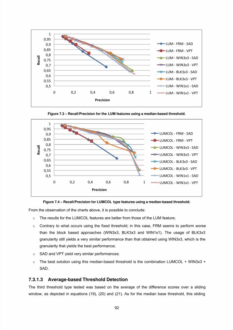
8/14/2019 H.264 Compressed Shot Detection
http://slidepdf.com/reader/full/h264-compressed-shot-detection 112/128
0,5
0,55
0,6
0,65
0,7
0,75
0,8
0,85
0,9
0,95
1
0 0,2 0,4 0,6 0,8 1
R e c a l l
Precision
LUM ‐ FRM ‐ SAD
LUM ‐ FRM ‐ VPT
LUM ‐ WIN3x3 ‐ SAD
LUM ‐ WIN3x3 ‐ VPT
LUM ‐ BLK3x3 ‐ SAD
LUM ‐ BLK3x3 ‐ VPT
LUM ‐ WIN1x1 ‐ SAD
LUM ‐ WIN1x1 ‐ VPT
Figure 7.3 – Recall/Precision for the LUM features using a median-based threshold.
0,5
0,55
0,6
0,65
0,7
0,75
0,8
0,85
0,9
0,95
1
0 0,2 0,4 0,6 0,8 1
R e c a l l
Precision
LUMCOL ‐ FRM ‐ SAD
LUMCOL ‐ FRM ‐ VPT
LUMCOL ‐ WIN3x3 ‐ SAD
LUMCOL ‐ WIN3x3 ‐ VPT
LUMCOL ‐ BLK3x3 ‐ SAD
LUMCOL ‐ BLK3x3 ‐ VPT
LUMCOL ‐ WIN1x1 ‐ SAD
LUMCOL ‐ WIN1x1 ‐ VPT
Figure 7.4 – Recall/Precision for LUMCOL type features using a median-based threshold.
From the observation of the charts above, it is possible to conclude:
o The results for the LUMCOL features are better from those of the LUM feature;
o Contrary to what occurs using the fixed threshold; in this case, FRM seems to perform worse
than the block based approaches (WIN3x3, BLK3x3 and WIN1x1). The usage of BLK3x3
granularity still yields a very similar performance than that obtained using WIN3x3, which is the
granularity that yields the best performance;
o SAD and VPT yield very similar performances;
o The best solution using this median-based threshold is the combination LUMCOL + WIN3x3 +
SAD.
7.3.1.3 Average-based Threshold Detection
The third threshold type tested was based on the average of the difference scores over a slidingwindow, as depicted in equations (19), (20) and (21). As for the median base threshold, this sliding
92

8/14/2019 H.264 Compressed Shot Detection
http://slidepdf.com/reader/full/h264-compressed-shot-detection 113/128
window is centered on the difference score being analyzed and does not include the current score. For
these tests, some values were made constant, notably: N = 4, T min = 0, T max = 1, a = 0 , c = 0 .
The performance results obtained for this type of threshold are depicted in Figure 7.5 and Figure 7.6.
As for the case of the median-based threshold, the parameter that was changed to generate the
charts was the multiplying constant (b).From the observation of these charts, it is possible to conclude:
o The results for the LUMCOL features are better from those of the LUM feature;
o The WIN3x3 granularity yields the best results. The usage of BLK3x3 granularity still yields a
very similar performance than that obtained using WIN3x3. FRM seems to perform worse than
the block based approaches.
o SAD and VPT yield very similar performances;
o The best solution using this average-based threshold is the combination LUMCOL + WIN3x3 +
SAD.
0,6
0,65
0,7
0,75
0,8
0,85
0,9
0,95
1
0 0,2 0,4 0,6 0,8 1
R e c a l l
Precision
LUM ‐ FRM ‐ SAD
LUM ‐ FRM ‐ VPT
LUM ‐ WIN3x3 ‐ SAD
LUM ‐ WIN3x3 ‐ VPT
LUM ‐ WIN1x1 ‐ SAD
LUM ‐ WIN1x1 ‐ VPT
LUM ‐ BLK3x3 ‐ SAD
LUM ‐ BLK3x3 ‐ VPT
Figure 7.5 - Recall/Precision the LUM features using an average-based threshold.
7.3.1.4 Comparison of the Different Threshold Approaches
Having presented the results for the three threshold types separately, this section intends to compare
the performances obtained. From Figure 7.7, which depicts the best results obtained by each type of
threshold, it is possible to conclude that the best overall detection performance is achieved, for all the
precision values, by both the median and average approaches, which yield similar results.
7.3.2 Second Phase: Transition Detection Performance
In this section the results of the tests performed on the second phase algorithms will be presented.
These tests were carried out by ignoring the first phase, i.e., by considering all GOPs in the videos as
suspects. The tests will be presented organized first by the dataset profile used and then by transition
type.
93

8/14/2019 H.264 Compressed Shot Detection
http://slidepdf.com/reader/full/h264-compressed-shot-detection 114/128
0,6
0,65
0,7
0,75
0,8
0,85
0,9
0,95
1
0 0,2 0,4 0,6 0,8 1
O v e r a l l R
e c a l l
Precision
LUMCOL ‐ FRM ‐ SAD
LUMCOL ‐ FRM ‐ VPT
LUMCOL ‐ WIN3x3 ‐ SAD
LUMCOL ‐ WIN3x3 ‐ VPT
LUMCOL ‐ WIN1x1 ‐ SAD
LUMCOL ‐ WIN1x1 ‐ VPT
LUMCOL ‐ BLK3x3 ‐ SAD
LUMCOL ‐ BLK3x3 ‐ VPT
Figure 7.6 - Recall/Precision for the LUMCOL features using the average-based threshold.
0,5
0,55
0,6
0,65
0,7
0,75
0,8
0,85
0,9
0,95
1
0 0,2 0,4 0,6 0,8 1
O V e r a l l R e c a l l
Precision
LUMCOL ‐ FRM ‐ VPT ‐ FIX
LUMCOL ‐ WIN3x3 ‐ SAD ‐
MED
LUMCOL ‐ WIN3x3 ‐ SAD ‐ AV
Figure 7.7 - Recall/Precision using the various proposed threshold approaches for the LUMCOL features.
7.3.2.1 Baseline Profile
The performance results achieved by all implemented algorithms will be presented next; first, for the
abrupt transition detection and, afterwards, for the gradual transition detection.
Abrupt Transition DetectionIn the context of abrupt transition detection, the procedures for the algorithms implemented can be
grouped between those which process only P frames (PHD in algorithms 1 and 2 and Inter in
algorithms 3 and 4) and those which also use IDR frames (Intra in Algorithm 3 and 4).
Figure 7.8 shows the results obtained for abrupt transition detection by the algorithms which only use
P frames. From the analysis of this chart, one can conclude that:
o The Recall seems to have a maximum possible at about 92%. This is due to the IDR frames, as
transitions between P and IDR cannot be detected by any of these algorithms.
o PHD absolute differences perform better than non-absolute differences, as it was described by
the authors.
94

8/14/2019 H.264 Compressed Shot Detection
http://slidepdf.com/reader/full/h264-compressed-shot-detection 115/128

8/14/2019 H.264 Compressed Shot Detection
http://slidepdf.com/reader/full/h264-compressed-shot-detection 116/128
0
0,01
0,02
0,03
0,04
0,05
0,06
0,07
0 0,2 0,4 0,6 0,8
R e c a l l
Precision
LUM ‐ WIN3x3
LUMCOL ‐ WIN3x3
LUMPART ‐ WIN3x3
Figure 7.9 – Recall / Precision for abrupt transition detection for the spatial differences (Intra procedure)
using a fixed threshold in Baseline profile.
The IBR detector is has four parameters that need to be set. For algorithm 1, only maxGTsize was
made constant; this was set to a very high value, since over the dataset the lengths of the gradual
transitions vary considerably and the false positives rejected by setting this parameter were not
significant. The T IBR , minGTsize and Δ were the test variables used to generate the results. As for
algorithm 2, minGTsize and Δ were also made constant (minGTsize=5 and Δ=2 ). Figure 7.10 shows
the performance of IBR at detecting gradual transitions for different parameters. However, since short
gradual transitions are considered abrupt, as referred in Section 7.2, another chart is shown in Figure
7.11 displaying the performance of IBR in detecting all transitions, which is needed to do a more
accurate assessment of the results obtained using the different parameters.
From the analysis of these charts, one may note that:
o In algorithm 1, the first parameter configuration, which is that proposed by the authors perform
worse than the others. As for the two remaining configurations, the main difference is in the
short gradual transition detection; the configuration with a lower minGTsize detects more of
these transitions for low thresholds but detects more false short gradual transitions for high
thresholds. This leads to a decrease in precision when the threshold is raised. However, as
short gradual transitions are only a few, that difference is not very significant.
o Between the two algorithms, one may conclude that the concatenation of gradual transitions
proposed improves the precision for gradual transition detection.
7.3.2.2 Main Profile
In this section, the performance results achieved by algorithms 2, 3 and 4, while processing bit
streams encoded in Main profile will be presented. The results for these algorithms will be presented
next; first for the abrupt transition detection and, afterwards, for the gradual transition detection
96

8/14/2019 H.264 Compressed Shot Detection
http://slidepdf.com/reader/full/h264-compressed-shot-detection 117/128
0
0,05
0,1
0,15
0,2
0,25
0,3
0,35
0,4
0,45
0,5
0 0,1 0,2 0,3 0,4 0,5
R e c a l l
Precision
Alg.1: Δ=1, minGTsize=4
Alg.1: Δ=2, minGTsize=4
Alg.1: Δ=2, minGTsize=5
Alg.2: Δ=2, minGTsize=5
Figure 7.10 - Recall/Precision for the gradual transition detection by the IBR approach with different
parameter settings in Baseline profile.
0
0,01
0,02
0,03
0,04
0,05
0,06
0 0,1 0,2 0,3 0,4
R e c a l l
Precision
Alg1: Δ=1, minGTsize=4
Alg.1: Δ=2, minGTsize=4
Alg.1: Δ=2, minGTsize=5
Alg.2: Δ=2, minGTsize=5
Figure 7.11 - Recall/Precision for the overall transition detection by the IBR approach with differentparameter settings in Baseline profile.
Abrupt Transition Detection
In order to detect abrupt transitions in videos encoded in the Main profile, there were presented three
algorithms relying of inter coded frames and one, which as in the baseline profile, tackles the problem
of IDR frames.
In Figure 7.12, the results for the various abrupt detection procedures relying on temporal
dependencies are shown.
From the analysis of this chart, one may conclude that:
o The PHD is that which performs the worse. In fact, it yields to much false positives even when
compared to the Inter procedure in Alg.3.
o The hierarchical approach introduced in Alg.4 improved the detection results significantly when
compared to Alg.3.
97

8/14/2019 H.264 Compressed Shot Detection
http://slidepdf.com/reader/full/h264-compressed-shot-detection 118/128
0,5
0,55
0,6
0,65
0,7
0,75
0,8
0,85
0,9
0,95
1
0,4 0,5 0,6 0,7 0,8 0,9 1
R e c a l l
Precision
Alg.2 ‐ PHD ‐ Non‐Abs.
Differences
Alg.3 ‐ Inter
Alg.4 ‐ Inter ‐ Only Tinter
Alg.4 ‐ Inter ‐ Tintepr = 0,3
Figure 7.12 - Precision / Recall for the abrupt transition detection relying on temporal dependencies in
Main profile.
o The introduction of the peak detector threshold (T inter2 ), to compare P frames from the base
layer, improved the precision over usage of the T inter threshold for that purpose, which only
detects high usage of intra coded macroblocks in these frames.
As for the performance of the intra procedures, in the preliminary testing LUMCOL still yielded better
results than the other features. Besides, this procedure seems to work better in this kind of sequences
than it did in the Baseline profile.
Gradual Transition Detection
For the detection of gradual transitions, the same procedure was used for all algorithms, for the same
reasons as in the Baseline profile. Two tests were carried out to compare two different settings; the
T IBR , minGTsize and Δ were the test variables used to generate the results. Figure 7.13 shows the
performance of IBR at detecting gradual transitions for different parameters. However, since short
gradual transitions are considered abrupt, as referred in Section 7.2, another chart is shown in Figure
7.14 displaying the performance of IBR in detecting all transitions, which is needed to do a more
accurate assessment of the results obtained using the different parameters.
From the analysis of the results in Figure 7.13 and in Figure 7.14 on may conclude that:
o minGTsize = 4 seems to perform slightly better than minGTsize = 5, detecting more transitions
without losing precision. This difference, however, is not significant.
98

8/14/2019 H.264 Compressed Shot Detection
http://slidepdf.com/reader/full/h264-compressed-shot-detection 119/128
0
0,1
0,2
0,3
0,4
0,5
0,6
0 0,05 0,1 0,15 0,2 0,25 0,3
Alg.2: Δ=2, minGTsize=4
Alg.2: Δ=2, minGTsize=5
Figure 7.13 - Recall/Precision for the gradual transition detection by the IBR approach with different
parameter settings in Main profile.
0
0,01
0,02
0,03
0,04
0,05
0,06
0 0,05 0,1 0,15 0,2 0,25 0,3
Alg.2: Δ=2, minGTsize=4
Alg.2: Δ=2, minGTsize=5
Figure 7.14 - Recall/Precision for overall transition detection by the IBR approach with different parametersettings in Main profile.
Overall System Performance
After the analysis of the performance of first and second phases, in the following some results are
presented about the two-phase overall system in Table 7.1. To obtain these results the followingparameters were set:
o First Phase – LUMCOL features; WIN3x3 granularity; SAD score and average-based threhold.
o Second Phase – Algorithm 4;
Inter procedure : Tinter = 0,7; Tinterp = 0,3.
Intra procedure: WIN3x3; LUMCOL; Tintra = 0,55.
Grad procedure: Tgrad = 0,6; minGTsize = 5; Δ = 2.
99

8/14/2019 H.264 Compressed Shot Detection
http://slidepdf.com/reader/full/h264-compressed-shot-detection 120/128
Table 7.1 - Some performance results for the developed system.
First PhaseOverall System
Overall Abrupt Gradual
Recall PrecisionSuspect
GOPs (%)Recall Precision Recall Precision Recall Precision
b=0 100% 5,9% 100% 85% 84,7% 90,5% 91,1% 25,2% 22,6%
b=0,95 99,5% 9,3% 62,3% 84,6% 85,3% 90,1% 91,6% 25,2% 23,1%b=1,1 95,2% 32,6% 17% 81,9% 89,3% 87,4% 93,3% 21,4% 30,6%
In this chapter, the dataset and the evaluation procedures used to test the various implemented shot
transition detection algorithms were described; afterwards, the results obtained each algorithm were
presented.
100

8/14/2019 H.264 Compressed Shot Detection
http://slidepdf.com/reader/full/h264-compressed-shot-detection 121/128
CHAPTE
Conclusions and
Future Work
R 8
ns of the work described in this document and some suggestions for future work on this
subject.
video directly in the compressed
the
This chapter finalizes the report by presenting a summary of the addressed topics, the main
conclusio
8.1 Summary and Conclusions
Chapter 1 introduced the motivations for the problem addressed in this Thesis; mainly due to the
increase in the digital video availability, applications providing means to browse and consume large
video collections, such as content-based video retrieval and summarization applications, are gaining
relevance. As shot detection is one of the fundamental steps of these types of applications; it is a
problem which needs to be addressed and resolved. Moreover, as digital video is usually compressed;
if shot transition detection is performed directly in the compressed domain, i.e., without having to
decompress the video, a significant reduction of computational complexity can be achieved. Amongthe video coding standards, H.264/AVC is the latest standard and its popularity is growing. This
standard achieves great compression efficiency at the cost of increased complexity, when compared
to previous standards, which strengths the need for processing the
domain. A short overview on this standard is provided in Chapter 2.
Chapter 3 structured and presented the shot detection problem and the solutions found among
relevant literature. Some of the most relevant solutions found were also described in more detail.
In Chapter 4 the developed system for shot detection was first introduced. This chapter described the
system architecture and provided a functional description of each of its modules. It is also motivated
the decision to adopt an hierarchical procedure, as suggested in [35], based on first detecting the
101

8/14/2019 H.264 Compressed Shot Detection
http://slidepdf.com/reader/full/h264-compressed-shot-detection 122/128
GOPs suspect of having transitions (suspect GOP detection) and, afterwards, analyzing those GOPs
more thoroughly, in order to find the exact placement of transitions (transition detection).
Chapter 5 described in detail the various processing algorithms developed in each of the system’s
modules to perform the shot transition detection. For the suspect GOP detection phase, the algorithm
in [35] was implemented, along with some modifications proposed by the author to test differentapproaches. For the transition detection phase, four algorithms were designed. The first algorithm is
that proposed in [34]; it compares successive inter frames using their partition sizes and types and the
second is an improvement of this first algorithm. The third algorithm was based on [16]; it inspects
intra prediction modes and the direction the used reference frames and it was designed to compare
successive frames in a sequential way, as happens in algorithms 1 and 2. The fourth algorithm was
based on the hierarchical detection also proposed in [16], with some modifications proposed by the
author of this Thesis; it analyses frames using the same features as in algorithm 3, but it does so in a
and explained.
hapter 7 presented a comparison of the results obtained for the several implemented algorithms,
and implementation of a shot
allowed several GOPs to
direction to be used and, although a solution is proposed
in [16], it is still a problem needing a better solution, since it is the main problem limiting the
nsition detection.
different order, exploiting the hierarchical reference usage. This is done to analyze less frames and to
improve the detection accuracy.
Chapter 6 intended to provide the reader with some relevant implementation details of the developed
system. The GUI developed for this system is also presented
C
over a representative dataset adopted from TRECVID 2007.
This work aimed mainly at designing, implementing, evaluation and comparison of shot transition
solutions in the H.264/AVC compressed domain and the designed
transition detection application. With this purpose algorithms in [35], [34] and [16] were implemented,
along with some modifications proposed by the author of this Thesis.
For the suspect GOP detection phase, the obtained results were below those expected and reported
in the original algorithm [35]. Despite that fact, the introduction of this phase
be skipped from a detailed analysis in the second phase. Many modifications were proposed to the
original algorithm which yielded improvements in the algorithm performance.
For the transition detection phase, four algorithms were implemented. Many conclusions can be drawn
from the tests carried out and the presented results. Namely, inspecting inter partitions sizes does not
yield better performance detection when compared to the simpler analysis of inter prediction direction.
Also, the usage of hierarchical detection inside the GOP improves performance over analyzing
successive frames. Finally, there are two main aspects which may need a more proper solution; first,
gradual transitions are very difficult to detect based only on the ratio of intra prediction usage; second,
the usage of IDR frames limit the prediction
performance of abrupt tra
102

8/14/2019 H.264 Compressed Shot Detection
http://slidepdf.com/reader/full/h264-compressed-shot-detection 123/128
8.2 Future Work
The solution presented in this document still leaves room for improvement and, as referred previously,
there are still problems which need to be resolved. Some aspects which may worth considering in
future work on this subject are:
o Improvement of gradual transition detection – Gradual transition detection is the main
difficulty of these algorithms. To improve the detection of this kind of transitions, there are more
sition detection evolving IDR frames – As referred, IDR frames
introduce constrains in the prediction chain which can be confused as abrupt transitions.
Faster low-level extraction – The low-level features extraction was based on the Reference
to test the algorithms. Moreover, the usage of this kind of
nisms should be
In conclusion, it seems like the algorithms operating in the H.264/AVC compressed domain do not
chieve very high recall/precision scores, as those reported in the uncompressed domain. However,
their performance is acceptable, considering the reduction in computational complexity, and there is
still room for improvements, which can be made to improve the performance of these algorithms.
features which can be used to improve the performance, e.g., the usage of weighted prediction
in B frames. The incorporation of features available at higher levels of decoding complexity can
also be studied more thoroughly, regarding the trade-off between the achieved improvement in
detection performance and increase in the detection complexity.
o Improvement of tran
Although a solution to solve this problem has already been suggested, there is still room for
improvement using different thresholds or similarity scores. In adaptive GOP structures, the
GOP length can also be considered, as the encoder may try to use IDR frames, mainly, where a
shot transition occurs.
o
Software provided by the JVT. This is not an optimal solution regarding computational
complexity, since it is not an objective of this software. Therefore, the replacement of the
module or improvements on the implemented module, regarding its functioning on this particular
context, can be done to improve the performance.
o Auto threshold – Setting the fixed thresholds needed to various decision processes
heuristically is a tedious and time-consuming task. Therefore, automatic (machine learning)
classifiers may be implemented
classifiers is usually associated with an improvement in performance.
o Suspect GOP phase improvement – The suspect GOP detection phase yields many false
positives. In this context a different similarity scores or classification mecha
studied to improve this subject.
o Detector for short gradual transitions – The TRECVID evaluation introduces the, so-called,
short gradual transitions. The design and implementation of a specific procedure to detect these
transitions can result in an improvement in detection accuracy.
o Extensive Performance Evaluation – The H.264/AVC encoding is used in several different
environments and, therefore, the encoding options used may vary significantly, e.g., adaptive
GOP structures, different bitrates, and higher resolutions; therefore, the algorithms should also
be evaluated using differen ng options and, eventually, adapted to each situation.t encodi
a
103

8/14/2019 H.264 Compressed Shot Detection
http://slidepdf.com/reader/full/h264-compressed-shot-detection 124/128
104

8/14/2019 H.264 Compressed Shot Detection
http://slidepdf.com/reader/full/h264-compressed-shot-detection 125/128
R
[1] YouTube - Broadcast Yourself; http://www.youtube.com.
[2] nd
Systems for Video Technology , vol. 17, nº 2, pp. 168-186, Feb. 2007.
[3] ction: unraveled and resolved?”, IEEE Transactions on Circuits
and Systems for Video Technology, , vol. 12, nº 2, pp. 90-105, Feb. 2002.
[4] nsactions on
Circuits and Systems for Video Technology , vol. 15, nº 3, pp. 365-377, Mar. 2005.
[5]
Systems for Video Technology, vol. 17, nº 4, pp. 483-489,Apr. 2007.
[6]
[7] r, and W. Kraaij, “Evaluation campaigns and TRECVid”, 8th ACM
[8]
Technology , vol. 13, nº 7, pp. 560-576, Jul. 2003.
[10] sociated audio for digital storage media at up
[11] res and associated
[12] “ITU-T
[13] “ISO/IEC 14496-2: "Information technology -- Coding of audio-visual objects -- Part 2: Visual",
2001.
eferences
J. Yuan et al., “A formal study of shot boundary detection”, IEEE Transactions on Circuits a
A. Hanjalic, “Shot-boundary dete
G. Boccignone et al., “Foveated shot detection for video segmentation”, IEEE Tra
C. Grana and R. Cucchiara, “Linear transition detection as a unified shot detection approach”,
IEEE Transactions on Circuits and
“ISO/IEC 14496-10: Advanced Video Coding.”
A. F. Smeaton, P. Ove
International Workshop on Multimedia Information Retrieval , CA, USA: 2006, pp. 321-330.
T. Wiegand et al., “Overview of the H.264/AVC video coding standard”, IEEE Transactions on
Circuits and Systems for Video
[9] “ITU-T Recommendation H.261: "Video codec for audiovisual services at p x 64 kbit/s”, Mar.
1993.
“ISO/IEC 11172: Coding of moving pictures and as
to about 1,5 Mbit/s”, 1993.
“ISO/IEC 13818: Information technology - Generic coding of moving pictu
audio information: Video.” 1996.
Recommendation H.263: "Video coding for low bit rate communication", 1996.
105

8/14/2019 H.264 Compressed Shot Detection
http://slidepdf.com/reader/full/h264-compressed-shot-detection 126/128
[14] J. Ostermann et al., “Video coding with H.264/AVC: tools, performance, and complexity”, IEEE
Circuits and Systems Magazine, vol. 4, nº 1, pp. 7-28, First Quarter 2004.
H. Schwarz, D. Marpe, and T. W[15] iegand, “Analysis of Hierarchical B Pictures and MCTF”, IEEE
tion, vol. 23, nº 7, pp. 473-489,
[17]
cessing , Chicago, IL, USA: 1998, pp. 884-887
[18] tistical models of video structure for content analysis and
[19] tion interface,
[20] n
[21]
”, International Conference on Acoustics, Speech, and Signal Processing , pp.
[22] e
actions on Multimedia, vol. 5, nº 1,
pp. 106-117, Mar. 2003.
[23] Z. Cernekova, I. Pitas, and C. Nikou, “Information theory-based shot cut/fade detection and
ems for Video Technology , vol.
[24] h, and D.R. Bull, “A unified approach to scene change
tation of video using frame and histogram space”,
30-140, Feb. 2006.
Sung Woo Choi, “Fast scene change detection using
direct feature extraction from MPEG compressed videos”, IEEE Transactions on Multimedia,
International Conference on Multimedia and Expo, Toronto, Ontario, Canada: 2006, pp. 1929-
1932.
[16] S. De Bruyne et al., “A compressed-domain approach for shot boundary detection on
H.264/AVC bit streams”, Signal Processing: Image Communica
Aug. 2008.
M. R. Naphade et al., “A high-performance shot boundary detection algorithm using multiple
cues”, International Conference on Image Pro
vol.1.
N. Vasconcelos and A. Lippman, “Sta
characterization”, IEEE Transactions on Image Processing , vol. 9, nº 1, pp. 3-19, Jan. 2000.
P. Salembier and T. Sikora, Introduction to MPEG-7: Multimedia content descrip
John Wiley & Sons, Inc., 2002.
J. Bescos, “Real-time shot change detection over online MPEG-2 video”, IEEE Transactions o
Circuits and Systems for Video Technology , vol. 14, nº 4, pp. 475-484, Apr. 2004.
Z. Cernekova, C. Kotropoulos, and I. Pitas, “Video shot segmentation using singular value
decomposition
181-184, vol. 3, Hong Kong: 2003.
D. Lelescu and D. Schonfeld, “Statistical sequential analysis for real-time video scene chang
detection on compressed multimedia bitstream”, IEEE Trans
video summarization”, IEEE Transactions on Circuits and Syst
16, nº 1, pp. 82-91, Jan. 2006.
W.A.C. Fernando, C.N. Canagaraja
detection in uncompressed and compressed video”, IEEE Transactions on Consumer
Electronics, vol. 46, nº 3, pp. 769-779, Aug. 2000.
[25] R.A. Joyce and B. Liu, “Temporal segmen
IEEE Transactions on Multimedia, vol. 8, nº 1, pp. 1
[26] Seong-Whan Lee, Young-Min Kim, and
vol. 2, nº 4, pp. 240-254, Dec. 2000.
106

8/14/2019 H.264 Compressed Shot Detection
http://slidepdf.com/reader/full/h264-compressed-shot-detection 127/128
[27] Chung-Lin Huang and Bing-Yao Liao, “A robust scene-change detection method for video
Technology , vol. 11, nº
12, pp. 1281-1288, Dec. 2001.
[28] B.-L. Yeo and B. Liu, “Rapid scene analysis on compressed video”, IEEE Transactions on
4, Dec. 1995.
TRECVID Video
ermany: 2007.
atesh, “New enhancements to cut, fade, and dissolve
th ACM international conference on Multimedia,
pp. 219-227, Marina del Rey, CA, USA: 2000.
[31] R. Lienhart, “Reliable dissolve detection”, Storage and Retrieval for Media Databases 2001, pp.
001.
[32] R. Lienhart, “Reliable transition detection in videos: a survey and practitioner's guide”,
International Journal of Image and Graphics, vol. 1, nº 3, pp. 469-486, Jul. 2001.
[33] K. Schöffmann and L. Böszörmenyi, “Early Stage Shot Detection for H.264/AVC Bitstreams”,
Technical Report , Jul. 2007; http:// www-itec.uni-klu.ac.at/~klschoef/papers/shotdetection.pdf.
[34] K. Schöffmann and L. Böszörmenyi, “Fast segmentation of H.264/AVC bitstreams for on-
demand video summarization”, 14th International Multimedia Modeling Conference, Kyoto,
Japan: 2008.
[35] Y. Liu et al., “A novel compressed domain shot segmentation algorithm on H.264/AVC”,
International Conference on Image Processing 2004., Singapore: 2004, pp. 2235-2238 Vol. 4.
[36] Apple QuickTime Pro; http://www.apple.com/quicktime/pro/.
[37] L. Aimar et al., x264 - a free h264/avc encoder; http://www.videolan.org/developers/x264.html.
[38] Nero Digital; www.nero.com/enu/technologies-nerodigital.html.
[39] H. Heijmans, “Composing morphological filters”, Image Processing, IEEE Transactions on, vol.
6, nº 5, pp. 713-723, May. 1997.
[40] S. Jeannin and A. Divakaran, “MPEG-7 visual motion descriptors”, Circuits and Systems for
Video Technology, IEEE Transactions on, vol. 11, Jun. 2001, pp. 720-724.
[41] “ISO/IEC 14496-14: The MP4 File Format.”
[42] “ISO/IEC 14496-12: ISO Base Media File Format.”
[43] “ISO/IEC 14496-15: AVC File Format.”
[44] “Apple - QuickTime - HD Gallery”; http://www.apple.com/quicktime/guide/hd/.
[45] “Visual C#”; http://msdn.microsoft.com/en-us/vcsharp/default.aspx.
[46] “.NET Framework”; http://msdn.microsoft.com/netframework.
segmentation”, IEEE Transactions on Circuits and Systems for Video
Circuits and Systems for Video Technology , vol. 5, nº 6, pp. 533-54
[29] J. Yuan et al., “THU-ICRC at TRECVID 2007”, International Workshop on
Summarization, pp. 79-83, Augsburg, Bavaria, G
[30] B. T. Truong, C. Dorai, and S. Venk
detection processes in video segmentation”, 8
219-230, San Jose, CA, USA: 2
107

8/14/2019 H.264 Compressed Shot Detection
http://slidepdf.com/reader/full/h264-compressed-shot-detection 128/128
[47] DirectShow, Microsoft; http://msdn.microsoft.com/en-us/library/ms783323(VS.85).aspx.
[48] DirectShowNET Library; http://directshownet.sourceforge.net.
[49] Zedgraph; http://zedgraph.org/.
[50] GPAC Project on Advanced Content; http://gpac.sourceforge.net.
[51] H.264/AVC reference software - JM v13.2; http://iphome.hhi.de/suehring/tml/.
[52] Haali Media Splitter; http://haali.cs.msu.ru/mkv.
[53] CoreAVC; http://www.coreavc.com.
[54] MeGUI; http://sourceforge.net/projects/megui.
[55] MeWiki; http://mewiki.project357.com.
[56] AviSynth; http://avisynth.org.


![Prediction system for activity recognition with compressed€¦ · recognition, we encode each video using Mencoder [21] into five different compressed versions in H.264 format,](https://static.fdocuments.us/doc/165x107/600ef5c125ffaa427a1e9500/prediction-system-for-activity-recognition-with-compressed-recognition-we-encode.jpg)


