H Optimization MIMO Positive Position Feedback Based...
173
Multi-mode Active Vibration Control Using H ∞ Optimization MIMO Positive Position Feedback Based Genetic Algorithm by Zhonghui WU B.Eng(Electrical) School of Computer Science, Engineering and Mathematics, Faculty of Science and Engineering 31/03/2014 A THESIS SUBMITTED IN FULFILMENT OF THE REQUIREMENT FOR THE DEGREE OF MASTER OF ENGINEERING Adelaide, South Australia, 2014 © (Zhonghui WU, 2014)
Transcript of H Optimization MIMO Positive Position Feedback Based...
Multi-mode Active Vibration Control Using
H∞ Optimization MIMO Positive Position
Feedback Based Genetic Algorithm
by
Zhonghui WU B.Eng(Electrical)
School of Computer Science, Engineering and
Mathematics, Faculty of Science and Engineering
31/03/2014
A THESIS SUBMITTED IN FULFILMENT OF THE
REQUIREMENT FOR THE DEGREE OF
MASTER OF ENGINEERING
Adelaide, South Australia, 2014
© (Zhonghui WU, 2014)

i
Contents
Abstract ................................................................................................................................... xi
List of Abbreviations .............................................................................................................xii
Certification ............................................................................................................................ iii
Acknowledgement .................................................................................................................. iv
Introduction ............................................................................................................................... 1
1.1 Motivation ....................................................................................................................... 1
1.2 Research Methodology ................................................................................................... 2
1.3 Vibration Control of Structure ........................................................................................ 3
1.4 Active Vibration Control of Structure ............................................................................ 4
1.4.1 open-loop and closed-loop control ......................................................................................... 4
1.4.2 Feed-forward and Feedback Control ..................................................................................... 6
1.4.3 Wave Control and Modal Control .......................................................................................... 7
1.4.4 SISO Control and MIMO Control ......................................................................................... 9
1.4.5 Collocated Control and Uncollocated Control ....................................................................... 9
1.5 Modal Based Controller for Multi-mode Vibration Control ......................................... 10
1.5.1 Independent Modal Space Control (IMSC) ......................................................................... 10
1.5.2 Resonant Control ................................................................................................................. 11
1.5.3 Positive Position Feedback (PPF) Control ........................................................................... 11
1.6 Plate or Shell Structure Vibration Control .................................................................... 16
1.7 Aim of the Thesis .......................................................................................................... 17
1.8 Outline of the Thesis ..................................................................................................... 18
Model of Flexible Plate Structure ........................................................................................... 20
2.1 Introduction ................................................................................................................... 20
2.2 Description of Experimental Plant ................................................................................ 22
2.3 Numerical Solution Using ANSYS .............................................................................. 25
2.3.1 Resonance Frequency ....................................................................................................... 26
2.3.2 Mode Shape ...................................................................................................................... 28
2.3.3 Harmonic Response Analysis ........................................................................................... 30
2.4 Simulation Model of The plate ..................................................................................... 35
2.5 Summary ....................................................................................................................... 44

ii
Spatial Norm and Model Reduction ....................................................................................... 45
3.1 Introduction ................................................................................................................... 45
3.2 Plate Model Reduction and Balanced Realization ........................................................ 45
3.2.1 SISO Plate Model Reduction and Balanced Realization ..................................................... 45
3.2.2 MIMO Plate Model Balanced truncation ............................................................................. 50
3.3 Summary ....................................................................................................................... 52
Model Correction .................................................................................................................... 53
4.1 Introduction ................................................................................................................... 53
4.2 Plate Correction Model ................................................................................................. 53
4.2.1 SISO Plate Model Correction .............................................................................................. 54
4.2.2 MIMO Plate Model Correction ............................................................................................ 56
4.3 Summary ....................................................................................................................... 62
Multi-mode SISO and MIMO PPF Controller ........................................................................ 63
5.1 Introduction ................................................................................................................... 63
5.2 PPF Controller Structure ............................................................................................... 64
5.3 PPF Controller Closed -loop Stability .......................................................................... 66
5.3.1 Scalar Case ........................................................................................................................... 66
5.3.2 Multivariate Case ................................................................................................................. 68
5.3.3 Multivariate PPF Controller implemented with feed-through plant .................................... 69
5.4 Multi-mode SISO and MIMO PPF Controller Parameter Selection ............................. 72
5.4.1 MATLAB Optimization toolbox and GA Optimization Search .......................................... 72
5.4.2 Multi-mode SISO PPF Controller Optimal Parameter Selection ......................................... 73
5.4.3 Multi-mode MIMO PPF Controller Optimal Parameter Selection ...................................... 76
5.5 Summary ....................................................................................................................... 77
Simulation ............................................................................................................................... 78
6.1 Multi-mode Three SISO PPF Controller Simulation .................................................... 78
6.2 Multi-mode MIMO PPF Controller Simulation ........................................................... 89
6.3 Summary ....................................................................................................................... 99
Experiment ............................................................................................................................ 101
7.1 Self-sensing ................................................................................................................. 101
7.2 Electronics .................................................................................................................. 102
iii
7.2.1 dSpace ................................................................................................................................ 102
7.2.2 Interfacing circuits ............................................................................................................. 103
7.2.3 Additional electronics ........................................................................................................ 104
7.3 Multi-mode SISO PPF Controller Experiment Implemented Result .......................... 105
7.4 Multi-mode MIMO PPF Controller Experimental Implemented Result .................... 122
7.5 Summary ..................................................................................................................... 139
Conclusion and Future Work ................................................................................................ 142
8.1 Outcomes of the Research .......................................................................................... 142
8.2 Future Work ................................................................................................................ 143
Bibliography ......................................................................................................................... 146

iv
List of Figures
Figure 2.1 A thin plate in transverse vibration ............................................................ 22
Figure 2.2 Transducer cross section (a) and model (b) ................................................ 23
Figure 2.3 System model shown in isometric view and side view ............................... 26
Figure 2.4 Modal Analysis mode shape of first mode ................................................. 28
Figure 2.5 Modal Analysis mode shape of second mode ............................................ 29
Figure 2.6 Modal Analysis mode shape of third mode ................................................ 29
Figure 2.7 Modal Analysis mode shape of forth mode ................................................ 29
Figure 2.8 Harmonic Analysis Example ........................................................................ 30
Figure 2.9 Amplitude Response of whole top plate to a harmonic disturbance at shaker ................................................................................................................................ 31
Figure 2.10 Phase Response of whole top plate to a harmonic disturbance at shaker . 31
(a) Transducer 1 resonant peaks .................................................................................... 32
(b) Transducer 1 resonance phase .................................................................................. 32
(c) Transducer 2 resonance peaks .................................................................................. 33
(d) Transducer 2 resonance phase .................................................................................. 33
(e) Transducer 3 resonance peaks .................................................................................. 34
(f) Transducer 3 resonance phase .................................................................................. 34
Figure 2.11 Simulated harmonic disturbance at shaker and measured resonant peaks and phase of top plate at transducer 1 (a, b), transducer 2 (c, d) and transducer 3 (e, f). ........................................................................................................................ 34
Figure 2.12 Block diagram representation of the PPF control problem .................... 35
Figure 2.13 three SISO (g11,g22,g33) 47 modes plate model ................................... 37
Figure 2.14 SISO (g11) 47 modes plate model at transducer 1 ................................. 38
Figure 2.15 SISO (g22) 47 modes plate model at transducer 2 ................................. 38
Figure 2.16 SISO (g33) 47 modes plate model at transducer 3 ................................. 39
Figure 2.17 MIMO 47 modes plate model ................................................................. 39
Figure 2.18 MIMO (Gp(1,1)) 47 modes plate model ................................................. 40

v
Figure 2.19 MIMO (Gp(1,2)) 47 modes plate model ................................................. 40
Figure 2.20 MIMO (Gp(1,3)) 47 modes plate model ................................................. 41
Figure 2.21 MIMO (Gp(2,1)) 47 modes plate model ................................................. 41
Figure 2.22 MIMO (Gp(2,2)) 47 modes plate model ................................................. 42
Figure 2.23 MIMO (Gp(2,3)) 47 modes plate model ................................................. 42
Figure 2.24 MIMO (Gp(3,1)) 47 modes plate model ................................................. 43
Figure 2.25 MIMO (Gp(3,2)) 47 modes plate model ................................................. 43
Figure 2.26 MIMO (Gp(3,3)) 47 modes plate model ................................................. 44
Figure 3.1 SISO Plate (g11) at transducer 1 Hankel singular values .......................... 46
Figure 3.2 SISO Plate (g11) at transducer 1 model reduction and balanced realization frequency domain compare .................................................................. 46
Figure 3.3 SISO Plate (g11) at transducer 1 model reduction and balanced realization singular values compare ....................................................................... 47
Figure 3.4 SISO Plate (g22) at transducer 2 Hankel singular values .......................... 47
Figure 3.5 SISO Plate (g22) at transducer 2 model reduction and balanced realization frequency domain compare .................................................................. 48
Figure 3.6 SISO Plate (g22) at transducer 2 model reduction and balanced realization singular values compare ....................................................................... 48
Figure 3.7 SISO Plate (g33) at transducer 3 Hankel singular values .......................... 49
Figure 3.8 SISO Plate (g33) at transducer 3 model reduction and balanced realization frequency domain compare .................................................................. 49
Figure 3.9 SISO Plate (g33) at transducer 3 model reduction and balanced Realization singular values compare ...................................................................... 50
Figure 3.10 MIMO Plate Hankel singular values ........................................................ 50
Figure 3.11 MIMO Plate model reduction and balanced realization frequency domain compare ..................................................................................................... 51
Figure 3.12 MIMO Plate model reduction and balanced realization singular values compare .................................................................................................................. 51
Figure 4.1 SISO plate model correction result ........................................................... 54
Figure 4.2 SISO plate (g11) model reduction result compare (balreal and correction).. 55
Figure 4.3 SISO plate (g22) model reduction result compare (balreal and correction)

vi
................................................................................................................................ 55
Figure 4.4 SISO plate (g33) model reduction result compare (balreal and correction) ................................................................................................................................ 56
Figure 4.5 MIMO plate model reduction result compare (balreal and correction) ........ 56
Figure 4.6 MIMO Plate model correction and balanced truncation singular values compare .................................................................................................................. 57
Figure 4.7 MIMO (Gpc(1,1)) plate model correction result ............................................ 57
Figure 4.8 MIMO (Gpc(1,2)) plate model correction result ............................................ 58
Figure 4.9 MIMO (Gpc(1,3)) plate model correction result ............................................ 58
Figure 4.10 MIMO (Gpc(2,1)) plate model correction result .......................................... 59
Figure 4.11 MIMO (Gpc(2,2)) plate model correction result .......................................... 59
Figure 4.12 MIMO (Gpc(2,3)) plate model correction result .......................................... 60
Figure 4.13 MIMO (Gpc(3,1)) plate model correction result .......................................... 60
Figure 4.14 MIMO (Gpc(3,2)) plate model correction result .......................................... 61
Figure 4.15 MIMO (Gpc(3,3)) plate model correction result .......................................... 61
Figure 5.1 Block Diagram of a Second-Order System with Positive Position Feedback ................................................................................................................................ 64
Figure 5.2 Bode Plot of a Typical PPF Filter Frequency Response Function .............. 65
Figure 5.3 Feedback control system associated with a flexible structure with ......... 70
Figure 5.4 multi-mode SISO PPF controller K11 optimal parameter result through GA search ...................................................................................................................... 74
Figure 5.5 multi-mode SISO PPF controller K22 optimal parameter result through GA search ...................................................................................................................... 74
Figure 5.6 multi-mode SISO PPF controller K33 optimal parameter result through GA search ...................................................................................................................... 75
Figure 5.7 multi-mode MIMO Controller optimal parameter result through GA search ...................................................................................................................... 76
Figure 6.1 SISO vibration control at transducer 1 (K11) open-loop and closed-loop impulse signal simulation result ............................................................................. 79
Figure 6.2 SISO vibration control at transducer 2 (K22) open-loop and closed-loop impulse signal simulation result ............................................................................. 79
vii
Figure 6.3 SISO vibration control at transducer 3 (K33)open-loop and closed-loop impulse signal simulation result ............................................................................. 80
Figure 6.4 SISO vibration control at transducer 1 (K11) open-loop and closed-loop step signal simulation result ................................................................................... 80
Figure 6.5 SISO vibration control at transducer 2 (K22) open-loop and closed-loop step signal simulation result ................................................................................... 81
Figure 6.6 SISO vibration control at transducer 3 (K33) open-loop and closed-loop step signal simulation result ................................................................................... 81
Figure 6.7 three SISO controller open-loop and closed-loop simulation result ........ 82
Figure 6.8 SISO vibration control at transducer 1 (K11) open-loop and closed-loop simulation result (1) ................................................................................................ 82
Figure 6.9 SISO vibration control at transducer 1(K11) open-loop and closed-loop simulation result (2) ................................................................................................ 83
Figure 6.10 SISO vibration control at transducer 2 (K22) open-loop and closed-loop simulation result (1) ................................................................................................ 83
Figure 6.11 SISO vibration control at transducer 2 (K22) open-loop and closed-loop simulation result (2) ................................................................................................ 84
Figure 6.12 SISO vibration control at transducer 3 (K33) open-loop and closed-loop simulation result (1) ................................................................................................ 84
Figure 6.13 SISO vibration control at transducer 3 (K33) open-loop and closed-loop simulation result (2) ................................................................................................ 85
Figure 6.14 MIMO Controller open-loop and closed-loop (Gwo(1,1),Gwc(1,1)) impulse signal simulation result at transducer 1 ................................................................. 90
Figure 6.15 MIMO Controller open-loop and closed-loop (Gwo(2,1), Gwc(2,1)) impulse signal simulation result at transducer 2 ................................................................. 90
Figure 6.16 MIMO Controller open-loop and closed-loop (Gwo(3,1), Gwc(3,1)) impulse signal simulation result at transducer 3 ................................................................. 91
Figure 6.17 MIMO Controller open-loop and closed-loop (Gwo(1,1), Gwc(1,1)) step signal simulation result at transducer 1 ................................................................. 91
Figure 6.18 MIMO Controller open-loop and closed-loop (Gwo(2,1), Gwc(2,1)) step signal simulation result at transducer 2 ................................................................. 92
Figure 6.19 MIMO Controller open-loop and closed-loop (Gwo(3,1), Gwc(3,1)) step signal simulation result at transducer 3 ................................................................. 92
Figure 6.20 MIMO Controller open-loop and closed-loop simulation result ................. 93

viii
Figure 6.21 MIMO Controller open-loop and closed-loop (Gwo(1,1), Gwc(1,1))simulation result (1) at transducer 1 ....................................................... 93
Figure 6.22 MIMO Controller open-loop and closed-loop (Gwo(1,1), Gwc(1,1))simulation result (2) at transducer 1 ....................................................... 94
Figure 6.23 MIMO Controller open-loop and closed-loop (Gwo(2,1), Gwc(2,1))simulation result (1) at transducer 2 ....................................................... 94
Figure 6.24 MIMO Controller open-loop and closed-loop (Gwo(2,1), Gwc(2,1))simulation result (2) at transducer 2 ....................................................... 95
Figure 6.25 MIMO Controller open-loop and closed-loop (Gwo(3,1), Gwc(3,1))simulation result (1) at transducer 3 ....................................................... 95
Figure 6.26 MIMO Controller open-loop and closed-loop (Gwo(3,1), Gwc(3,1))simulation result (2) at transducer 3 ....................................................... 96
Figure 7.1 principle of the self-sensing technique used to measure the back-emf voltage Vemf ........................................................................................................ 101
Figure 7.2 block diagram for the calculation of the back-emf voltage ...................... 102
Figure 7.3 The interface circuit used to power the control transducer and to measure .............................................................................................................................. 104
Figure 7.4 SISO vibration control at transducer 1 first mode 27.1 Hz before control .. 106
Figure 7.5 SISO vibration control at transducer 1 first mode 27.1 Hz after control ..... 106
Figure 7.6 SISO vibration control at transducer 1 second mode 34.4 Hz before control .............................................................................................................................. 107
Figure 7.7 SISO vibration control at transducer 1 second mode 34.4 Hz after control 107
Figure 7.8 SISO vibration control at transducer 1 third mode 40.5 Hz before control. 108
Figure 7.10 SISO vibration control at transducer 1 forth mode 49.2 Hz before control .............................................................................................................................. 109
Figure 7.11 SISO vibration control at transducer 1 forth mode 49.2 Hz after control . 109
Figure 7.28 SISO vibration control for sweep signal at transducer 1 before control ... 118
Figure 7.29 SISO vibration control for sweep signal at transducer 1 after control ...... 118
Figure 7.30 SISO vibration control for sweep signal at transducer 2 before control ... 119
Figure 7.31 SISO vibration control for sweep signal at transducer 2 after control ...... 119
Figure 7.32 SISO vibration control for sweep signal at transducer 3 before control ... 120

ix
Figure 7.33 SISO vibration control for sweep signal at transducer 3 after control ...... 120
Figure 7.58 MIMO vibration control for sweep signal at transducer 1 before control 136
Figure 7.59 MIMO vibration control for sweep signal at transducer 1 after control ... 136
Figure 7.61 MIMO vibration control for sweep signal at transducer 2 after control ... 137
Figure 7.63 MIMO vibration control for sweep signal at transducer 3 after control ... 138
Figure 8.1 Modal Analysis mode shape of first mode with four transducers ............ 144

x
List of Tables Table 2.1: Mechanical parameters of the transducers ................................................... 23
Table 2.2: Electrical parameters of the three transducers (T 1, 2 and 3) ....................... 24
Table 2.3: The first four natural frequencies of the experimental model ...................... 25
Table 2.4 natural frequencies comparison .................................................................. 27
Table 5.1 classical algorithm and genetic algorithm comparison .............................. 73
Table 5.2 multi-mode SISO PPF controller optimal parameter result ....................... 75
Table 5.3 multi-mode MIMO PPF controller optimal parameter result .................... 77
Table 6.1 SISO PPF closed-loop frequency domain result at transducer 1 ................ 86
Table 6.2 SISO PPF closed-loop frequency domain result at transducer 2 .................. 87
Table 6.3 SISO PPF closed-loop frequency domain result at transducer 3 ................ 88
Table 6.4 MIMO PPF closed-loop frequency domain result at transducer 1 ............ 97
Table 6.5 MIMO PPF closed-loop frequency domain result at transducer 2 ............ 98
Table 6.6 MIMO PPF closed-loop frequency domain result at transducer 3 ............ 99
Table 7.2 AD and DA converters on the dSpace DS1103 used for signal acquisition and reference voltage output ...................................................................................... 103
Table 7.3 specific measurement resistor value for each interface circuit ................. 104
Table 7.4 SISO vibration control experimental results .............................................. 121
Table 7.5 multi-mode SISO PPF controller experimental parameter result ............ 122
Table 7.6 multi-mode MIMO PPF controller parameter result ............................... 123
Table 7.7 multi-mode MIMO vibration control experimental results ....................... 139

xi
Abstract
In this thesis, experimental, analytical and numerical analysis three kinds of methods
are used for distributed parameter plate structure modeling, an infinite-dimensional
and a very high-order plate mathematical transfer function model is derived based on
modal analysis and numerical analysis results. A feed-through truncated plate model
which minimizing the effect of truncated modes on spatial low-frequency dynamics
of the system by adding a spatial zero frequency term to the truncated model is
provided and numerical software MATLAB is used to compare the feed-through
truncated plate model with traditional balanced reduction plate model which is used
to decrease the dimensions and orders of the infinite-dimensional and very high-order
plate model. Active vibration control strategy is presented for a flexible plate
structure with bonded three self-sensing magnetic transducers which guarantee
unconditional stability of the closed-loop system similar as collocated control system.
Both multi-mode SISO and MIMO control laws based upon positive position
feedback is developed for plate structure vibration suppression. The proposed
multi-mode PPF controllers can be tuned to a chosen number of modes and increase
the damping of the plate structure so as to minimize the chosen number of resonant
responses. Stability conditions for multi-mode SISO and MIMO PPF controllers are
derived to allow for a feed-through term in the model of the plate structure which is
needed to ensure little perturbation in the in-bandwidth zeros of the model. A
minimization criterion based on the H∞ norm of the closed-loop system is solved by
a genetic algorithm to derive optimal parameters of the controllers. Numerical
simulation and experimental implementation are performed to verify the
effectiveness of multi-mode SISO and MIMO PPF controllers vibration suppression
for the feed-through truncated plate structure.
xii
List of Abbreviations
SISO Single Input Single Output MIMO Multiple Input Multiple Output T.F Transfer Function PDE Partial Derivative Equation ODE Ordinary Differential Equation
PPF
Positive Position Feedback
IMSC Independent Modal FSS
Flexible Spacecraft Simulator AVA Active Vibration Absorber SRF Stain Rate Feedback LQR Linear Quadric Regulator NNP Neural Network Predictive LQG Linear Quadratic Gaussian
PACE Planar Articulating Controls Experiment
RCGA Real Coded Genetic Algorithm SIMO Single Input Multiple Output FXLMS
Filtered-X Least Mean Square AVC Active Vibration Control
MISO Multiple Input Single Output
FEM Finite Element Method MDF Medium Density Fibreboard

iii
Certification
I certify that this work does not incorporate without acknowledgment any material
previously submitted for a degree or diploma in any university; and that to the best
of my knowledge and belief it does not contain any material previously published or
written by another person except where due reference is made in the text.
Flinders University may lend this thesis to other institutions or individuals for
the purpose of scholarly research;
Flinders University may reproduce this thesis by photocopying or by other means,
in total or in part, at the request of other institutions or individuals for the purpose
of scholarly research.
Adelaide, 31 March 2014
Zhonghui WU

iv
Acknowledgement
I am heartily thankful to Associate Professor Fangpo He, whose guidance and
support at the initial and medium level.
To Dr. Lei Chen, who is from the mechanical engineering school of Adelaide
University, thanks a lot for your willingness to help and your availability time for
long discussions and helpful suggestions.
To S. O. R. Moheimani, thanks a lot for your contributions to vibration control
theory. I felt that I was just like under your supervision to finish my thesis after
read your books and thesis.
To Siyang Yu, thanks for your help and discussion the ANSYS model with me.
Finally, I wish to thank my family, my father-in-law, mother-in-law, my mum, and my
daughter Hanzhen , Hanen, especially to my wife Clare, whom I mostly in debt, thank
you so much for your constant love, support, patience, and encouragement during the
whole study time of master degree at Flinders University, without whom I would be
unable to complete my degree, thanks a million, love you forever!
Also thanks all the people who giving help:
Miss Natalie Hills
Ms Kylie Sappiatzer
Ms Vanesa Duran Racero
Prof Sonia Kleindorfer,
Professor Paul Calder,
Dr Peter Anderson,
Ms Anne Hayes
Ms Lisa O'Neill
Prof Mark Taylor
Prof John Roddick

v
Prof Warren Lawrance
Prof Carlene Wilson
Prof Jeri Kroll

1
Chapter 1
Introduction
This chapter discusses the motivation for the research described in this thesis. The
research methodology is presented, followed by a literature review. Finally, an outline
of the thesis is given along with a list of original contributions.
1.1 Motivation
In order to improve dynamic performance, the operating efficiency, and the amount of
material which is used in mechanical structures, many designers employ lightweight
materials to reduce the cross sectional dimensions of those structures [4].
However, one side-effect of employing lightweight materials and reducing the cross
sectional dimensions is that the structures become more flexible. Flexible structures are
more susceptible to the detrimental effects of unwanted vibration, particularly when
they operate at or near their natural frequencies or when they are excited by
disturbances that coincide with their natural frequencies [4].
The design and implementation of a high performance vibration controller for a flexible
structure can be a difficult task. The difficulty is due to the following factors but not
limited:
i. A major difficulty in control of flexible structures is due to the fact that they are
distributed parameter systems. Consequently, these structures have a very large
number of vibration modes and their transfer functions contain many poles close to
the jω axis [1]. High-frequency modes also contribute to the dynamics at low
frequencies. Thus, a model may have to include a relatively high number of high-f
requency modes to capture the low frequency dynamics with acceptable accuracy.
This yields a model with a relatively high order and the systems are generally
difficult to control [2].

2
ii. In most cases, a small number of in-bandwidth modes of the structure are required
to be controlled, and it is possible that some in-bandwidth modes are not targeted to
be controlled at all. The presence of uncontrolled modes can lead to the problem of
spill-over. That is, the control energy is channeled to the residual modes of the
system and this process may destabilize the closed-loop system. In particular, the
spill-over effect is of major concern at higher frequencies where obtaining a
precise model of the structure is rather difficult [3]. Normally there are two types
of spill-over: control spill-over and observation spill-over. Control spill-over
occurs when the control force excites unmodeled dynamics. The excitation of
these unmodeled dynamics can degrade the performance of the system.
Observation spill-over refers to the measurement error caused by the contribution
of excluded modes to the sensor measurements. While control spill-over leads to
poor performance, observation spill-over can lead to instability [4].
iii. To control a flexible structure that has widely separated multi-mode vibration a
wide-band controller is needed. However, the design of a high performance
wide-band controller is difficult. The difficulty is due to the design trade-off
between the error reduction in one frequency band and the increase of sensitivity
at other frequencies, as explained in Bode’s theorem [5] .
Given these requirements, the question is how to design and implement a suitable
controller. Seeking the answer to this questions is the motivation for the research
described in this thesis.
1.2 Research Methodology
The research methodology includes of four steps:
In the first step, a literature review overviews the relevant existing methods for
controlling the vibration of flexible structures, and discusses the relevant shortcomings
or gaps in those methods. Based on the gaps that are found in the existing methods, new
control methods are proposed.
In the second step, an experimental plant that can be used as a tool for the design and
evaluation of the effectiveness of the proposed control methods, is designed and
implemented. The plant chosen must represent a real application and have the essential

3
characteristics of a flexible structure. A flexible two dimensions plate with three
transducers which are treated as supporting feet is chosen as the experimental plant.
In the third step, analytical and numerical analysis three kinds of methods are used for
modeling, an infinite-dimensional and a very high-order plate mathematical transfer
function model is derived based on modal analysis and numerical analysis results. A
feed-through truncated system model which minimizing the effect of truncated modes
on spatial low-frequency dynamics of the system by adding a spatial zero frequency
term to the truncated system model is provided and numerical software MATLAB is
used to compare the feed-through truncated system model with traditional balanced
reduction model which is used to decrease the dimensions and orders of the
infinite-dimensional and very high-order model.
In the fourth step, SISO and MIMO PPF controllers were designed based on the H∞
norm of the closed-loop system by a genetic algorithm to derive optimal parameters
of the controller.
In the fifth step, simulation models of the experimental plant are implemented, and
computer simulations are exercised. These simulations reduce the design time, increase
the success rate of the real-time implementation, and help in the evaluation of the
performances of the proposed controllers prior to their use with the experimental plant.
In the sixth step, the proposed controllers are used with the experimental plant and the
effectiveness of the proposed control methods are evaluated.
1.3 Vibration Control of Structure
Vibration control is applied with respect to avoid the unwanted vibration of the
structure. Vibration control can be categorized into two major techniques: passive
control and active control.
Passive Control
For passive control, vibration is attenuated or absorbed by traditional vibration dampers,
shock absorbers, and base isolation. However, it has two major drawbacks.:

4
i. Firstly, it is ineffective at low frequencies. The natural frequency is inversely
proportional to the square root of the spring compliance and to the mass of the
damper. Hence, at low frequencies, the volume and mass requirements are often
impractically large for many applications where physical space and mass loading
are critical.
ii. Secondly, the passive technique only works effectively for a narrow band of
frequencies and is not easy to modify [6].
Active Control
For active vibration control, it is the active application of force in an equal and opposite
fashion to the forces imposed by external vibration.In contrast with passive control,
active control works effectively over a wide bandwidth where the working band does
not depend on the characteristics of the structure, and is limited only by the bandwidth
of the actuators. Furthermore, the actuators are less sensitive to the characteristics of the
structures and the vibration sources. Therefore, the same actuators can be used even if
the characteristics of the structures or the vibration sources are changed. To maintain
the system performance, the electronic controller might need to be modified, but this
modification is relatively easy, especially with digital controllers [7].
From the above discussion, it is clear that active control shows better potential
comparing with passive control. So this thesis will focus on the design of active
controllers.
1.4 Active Vibration Control of Structure
1.4.1 open-loop and closed-loop control
Active control can be classified as open-loop and closed-loop.
Open-loop Control
An open-loop control system uses a controller and an actuator to obtain the desired
response and it is a system without feedback [8]. In general, an open-loop system relies
on the model of the plant to obtain a command input that, supplied to it, causes the
output to follow a desired pattern. This strategy requires very good knowledge of the

5
dynamics of the controlled system and is usually applied only as a feed-forward
component in conjunction with a feedback controller [9].
advantages:
simplicity and stability: they are simpler in their layout and hence are economical
and stable too due to their simplicity.
construction: since these are having a simple layout so are easier to construct [9].
disadvantages:
accuracy and reliability: since these systems do not have a feedback mechanism, so
they are very inaccurate in terms of result output and hence they are unreliable too.
due to the absence of a feedback mechanism, they are unable to remove the
disturbances occurring from external sources [9].
Closed-loop Control
In contrast to an open-loop control system, a closed-loop control system utilizes an
additional measure of the actual output to compare the actual output with the desired
output response. The measure of the output is called the feedback signal. A feedback
control system is a control system that tends to maintain a prescribed relationship of
one system variable to another by comparing functions of these variables and using the
difference as a means of control. With an accurate sensor, the measured output is a
good approximation of the actual output of the system [8].
advantages:
accuracy: they are more accurate than open-loop system due to their complex
construction. They are equally accurate and are not disturbed in the presence of
non-linearities.
noise reduction ability: since they are composed of a feedback mechanism, so they
clear out the errors between input and output signals, and hence remain unaffected
to the external noise sources [8].
disadvantages:

6
construction: they are relatively more complex in construction and hence it adds up
to the cost making it costlier than open-loop system.
since it consists of feedback loop, it may create oscillatory response of the system
and it also reduces the overall gain of the system.
stability: it is less stable than open loop system but this disadvantage can be striked
off since we can make the sensitivity of the system very small so as to make the
system as stable as possible [8].
In order to achieve better performance, the design control method discussed in this
thesis will concentrate on closed-loop control.
1.4.2 Feed-forward and Feedback Control
Active control can be classified as feed-forward or feedback control depending on the
derivation of the error signal.
Feed-forward Control
Feed-forward is a term describing an element or pathway within a control system which
passes a controlling signal from a source in its external environment, often a command
signal from an external operator, to a load elsewhere in its external environment. A
control system which has only feed-forward behavior responds to its control signal in a
pre-defined way without responding to how the load reacts; it is in contrast with a
system that also has feedback, which adjusts the output to take account of how it affects
the load, and how the load itself may vary unpredictably; the load is considered to
belong to the external environment of the system [10].
In a feed-forward system, the control variable adjustment is not error-based. Instead it
is based on knowledge about the process in the form of a mathematical model of the
process and knowledge about or measurements of the process disturbances [10].
For the feed-forward system[11,12,13], it has some advantages [14]:
wider bandwidth
works better for narrow-band disturb
7
also include disadvantages [14]:
reference needed
local method (response may be amplified in some part of the system)
large amount of real time computations
Feedback Control
In feedback control, the error signal, which is the difference between the desired
response and the controlled output, is fed to the controller. The controller then
generates control signals to drive the error signal to zero. With feedback control,
stability becomes a major concern because the feedback modifies the characteristic of
the original plant [14].
advantages [14]:
guaranteed stability when collocated
global method
attenuates all disturbances within ωc (bandwith)
disadvantages [14]:
effective only near resonances
limited bandwidth
disturbances outside ωc (bandwith) are amplified
spill-over
Due to the excitation signal in the flexible plate, feed-forward control is not suitable for
application with this system. Therefore, the design control method discussed in this
thesis mainly focuses on feedback control.
1.4.3 Wave Control and Modal Control
Active control can also be classified according to the model descriptions upon which
the control design is based. The most common descriptions of the vibration of
continuous systems are in terms of waves and modes of motion [15]. These two
descriptions lead to two different approaches for active control: wave control and

8
modal control.
Wave Control
In a structure where the flow of vibrational energy from one part to another is
significant and needs to be reduced, wave control is normally used. Wave control
design makes use of the wave equation of a structure and the local properties at and
around the control region. Since inherently the local properties of the structure are less
sensitive to system properties wave control has a good robustness. However, because it
does not take into account global motion, global behaviour can adversely affect the
amount of control achieved [4].
Difficulty in realizing an active wave control system is that all components in the
system are expressed as non-causal and irrational functions of Laplace variable s.
Therefore, in a practical case, the wave controllers are approximately realized to a
limited extent [16].
Modal Control
Modal control of flexible structures has been of great interest for several decades
among vibration control engineers. In general, modal analysis and control refer to the
procedure of decomposing the dynamic equations of a system into modal coordinates
and designing the control system in this modal coordinate system [17]. The principle
behind it is that it somehow extracts a target mode signal from the structural response
and controls it in modal domain in a similar way to controlling a single
degree-of-freedom oscillator. Advantages are as follows: controller design is easy as it
is conducted in modal domain, a global vibration reduction over the whole structure can
be achieved by suppressing modes at a number of discrete positions (i.e., global control
using local feedback), and the designed controller is inherently very robust to the
dynamics of uncontrolled modes [18].
Because of the implement limitation, in this thesis, the design control method will
follow on collocated control.

9
1.4.4 SISO Control and MIMO Control
A single-input and single-output (SISO) system is a simple single variable control
system with one input and one output. Systems with more than one input and more than
one output are known as multi-input multi-output (MIMO) systems. Normally SISO
systems are typically less complex than MIMO systems, and SISO system is also easier
to be constructed and implemented.
Due to the increasing complexity of the system under control and the interest in
achieving optimum performance, the importance of control system engineering has
grown in the past decade. Furthermore, as the systems become more complex, the
interrelationship of many controlled variables must be considered in the control
scheme [4].
In order to make the clearly comparison, in this thesis, both SISO and MIMO methods
will be invested later.
1.4.5 Collocated Control and Uncollocated Control
Collocated Control
A collocated control system is a control system where the actuator and the sensor are
attached to the same d.o.f.(degree of freedom). It is not sufficient to be attached to the
same location; they must also be dual, that is, a force actuator must be associated with a
displacement (or velocity or acceleration) sensor, and a torque actuator with an angular
(or angular velocity) sensor, in such a way that the product of the actuator signal and the
sensor signal represents the energy (power) exchange between the structure and the
control system [3].
The structure of the collocated system allows for the design of feedback controllers,
with specific structures, that guarantee unconditional stability of the closed-loop
system. Such controllers are of interest due to their ability to avoid closed-loop
instabilities arising from the spill-over effect [3].
Uncollocated Control

10
Non-collocation of sensor and actuator is often unavoidable due to installation
convenience of transducers or is even recommendable for high degrees of observability
and controllability. However, non-collocated control is generally known to be more
involved than collocated control as the plants are no longer minimum phase [18].
For non-collocated control, one major reason for this is a modeling difficulty, since it is
impossible to model an infinite number of modes existing in a flexible structure. Those
controllers designed based on a few low order modes may thus seriously suffer from the
control spillovers associated with un-modeled but often non-negligible high order
modes. Another is due to the non-minimum phase characteristic of the plant, and thus
the modes excited by a control actuator will not all be the same in phase, when
measured at a non-collocated sensor location [18].
Based on the information, in this thesis, the design control method will pay close
attention on collocated control.
1.5 Modal Based Controller for Multi-mode Vibration
Control
There are three main modal control methods that can be found in the literature for
controlling multi-mode vibration in flexible structures: independent modal space
control (IMSC) , resonant control and positive position feedback (PPF) control.
1.5.1 Independent Modal Space Control (IMSC)
Meirovitch [19,20] established the independent modal space control (IMSC) which
allows the control design for each single mode to be implemented independently, hence
there is little spillover to the residual modes. However, this method requires as many
sensors/ actuators as the number of modes to be controlled, and thus it can only control
a limited number of modes. Furthermore, the control system is vulnerable to
uncertainties such as parameter fluctuation. To overcome this problem, the application
of the robust control techniques to active vibration control problem has been discussed
in the past two decades [16].

11
1.5.2 Resonant Control
The resonant control method proposed by Moheimani et al. [21,22,23,24,25,26] is
based on the resonant characteristic of flexible structures. The controller applies high
gain at the natural frequency and rolls off quickly away from the natural frequency thus
avoiding spillover. It is also described as having a decentralized characteristic from a
modal control perspective [27], thereby making it possible to treat each of the system’s
modes in isolation. One of the issues with resonant controllers is their limited
performance in terms of adding damping to the structure [3].
1.5.3 Positive Position Feedback (PPF) Control
Positive position feedback (PPF) was devised by Goh and Caughey [28,29], the
stability was proved by Fanson J. L. [30,31], it has several distinguished advantages
[32]. It has been shown to be a solid vibration control strategy for flexible systems with
smart materials, particularly with the PZT (lead zirconium titanate) type of
piezoelectric material [28,29,30].
PPF controller development
After the PPF controller theory was provided, lots of people did the simulations and
experiments using PPF theory for active vibration, for example:
[31] developed the method further and showed that PPF was capable of controlling the
first six bending modes of a cantilever beam. The second order PPF filter was simple to
implement and had global stability conditions, which were easy to fulfill even in the
presence of actuator dynamics.
[33,34] introduced a first order PPF filter eliminating one of the three filter parameters.
They also combined the positive position feedback with independent modal space
control.
[35] realized that effective vibration control with PPF depends on the accuracy of the
modal parameters used in the control design. They extended the original feedback
technique with an adaptive estimation procedure to identify the structural parameters.

12
[36] implemented PPF in both discrete and continuous systems, showed that an exact
knowledge of the natural frequencies of the structure is not required in order to design
an effective control system.
[37] presented the effectiveness of the optimal modal positive position feedback
algorithm in damping out two vibration modes of a cantilever beam with one
piezoelectric actuator and three position sensors.
[38] illustrated that an adaptive first order PPF filter can successful damp vibration of a
cantilever beam even if the first mode changes by 20%.
[39] provide PPF controller employing multiple actuators instead of a single one for
any particular vibration mode.
[40] designed a combined scheme of PD feedback controller for AC servo motor and
PPF controller for PZT actuators to suppress multi-mode vibration applied to
experimental single-link flexible manipulator.
[41] implemented a single mode PPF and also a multi-mode PPF controller under
single channel control scheme for vibration of beam
[42] introduced PPF to increase the stability margins and allow higher control
bandwidth, compensated for the coupled fuselage-rotor mode of a Rotary wing
Unmanned Aerial Vehicle (RUAV).
[43] PPF controllers are designed based on the identified results and investigated active
vibration control of a beam under a moving mass using a pointwise fiber Bragg grating
(FBG) displacement sensing system.
[44] indicated a multi-mode controllable SISO PPF controller, a non-collocated sensor/
moment pair actuator, and tuned to different vibration modes of beam based on the
results of the parametric study for the design parameters.
Modified PPF (MPPF)
based on the performance has already achieved, some researchers modify the structure
of PPF, [45] provided a modified compensator which enhanced flexibility actively
13
changing damping and stiffness of flexible structures. [46] constructed a new MPPF
which consists of first order and second order two SISO parallel compensators, and find
the optimal parameters through experimental way. [47] combined PPF and an output
feedback sliding mode control (AOFSMC) for vibration and attitude control. [48]
designed suboptimal positive position feedback (SOPPF) and output feedback sliding
mode control (OFSMC). [49] provided negative position feedback (NPF) and positive
position feedback (PPF) to reduce multi-mode vibration of a lightly damped flexible
beam using a piezoelectric sensor and piezoelectric actuators. [50] proposed positive
velocity and position feedback (PVPF) controller and achieved high-amplitude
actuation of a piezoelectric tube. [51] extended the linear modal control to nonlinear
modal control by using quadratic modal positive position feedback (QMPPF) control
algorithm to suppress forced vibrations in distributed parameter structures.
Robust PPF
Expect the normal advantages, some people also showed the robust ability of PPF
controller.
PPF control system is robust and performs significantly well at the target frequency,
because the high control action can be generated at the resonance of the controller due
to the tuning stated in literatures [52,53]. [54] presented the experimental results
robustness study of vibration suppression of a cantilevered beam with PZT sensors and
PZT actuators using PPF control. PPF controllers were implemented for single-mode
vibration suppression and for multimode vibration suppression. Experiments found
that PPF control is robust to frequency variations for single-mode and for multimode
vibration suppressions. [55] considered PPF which derived from solving a group of
LMIs with adjustable parameters with respect to the inaccurate structure modal
frequencies and a simulation was presented to illustrate the effectiveness of the
proposed robust PPF controller design method.
Adaptive PPF
In order to control vibration of structures with varying parameter, an adaptive PPF
controller was put into the consideration. [56] presented an adaptive modal control
algorithm, utilized only modal position signals, fed through first-order filters to damp

14
out the vibration, [57,58,59] proposed the use of GA for tuning PPF controller for grid
structure, [60] proposed a new APPF based on gradient-descent approach for beam
structure, [61] provided a SISO PPF controller with RLS and Bairstow combined
online frequency estimator, [62] designed a SISO PPF controller for a simulation study
with RLS estimator for the first two natural frequencies of a beam structure, [63,64]
developed RLS estimator with SISO PPF controller for the beam structure, [65]
through system identification, a two-mode SISO PPF controller was designed for beam
structure based on GA which was designed to minimize the H∞-norm and choose PPF
optimal parameters.
PPF combine with Genetic Algorithms (GA)
During the PPF controller design, in order to achieve better performance, some
designer used Genetic Algorithms (GA) to choose the placement of sensor and
actuator. [66] applied GA to find efficient location of sensor and actuator of a
cantilevered composite plate, showed significant vibration reduction for the first three
modes (controlled modes) has been observed using the coupled PPF in the vibration
control experiment. and the closed loop has been observed to robust with respect to
system parameter variations. [67] presented GA method of optimal placement for the
cantilever plate. Simulations and experimental results on the actual process have
shown that the proposed control method by combining PPF and PD can suppress the
vibration effectively, especially for vibration decay process and the smaller amplitude
vibration.
PPF compare with other controllers
In order to compare the performance with other controllers, some researchers did
simulations and experiments, such as [68] compared with AVA controller at SISO and
MIMO situation, [69] conducted simulations and experiments for SISO PPF case
compared with LQG controller for suppressing the single and multi- modes vibration of
flexible spacecraft simulator (FSS). [70] showed that a PPF controller may be
formulated as an output feedback controller both in centralized and decentralized
situation. [71,72,73,74] compared PPF with stain rate feedback(SRF), [75]compared
PPF with velocity feedback. [76] compared Positive position feedback (PPF) control,
linear quadric regulator (LQR) control and neural network predictive (NNP) control

15
strategies. [77] compared negative imaginary feedback controllers (PPF, Resonant
Controllers, Integral Resonant Controllers) with state feedback controller. [78]
compared velocity feedback controller, the integral resonant controller (IRC), the
resonant controller, and the positive position feedback (PPF) controller. [79] gave a
PPF controller for controlling the first mode of vibration, a decentralized controller
which used three independent PPF filters for suppressing the first three modes of
vibration and a MIMO linear quadratic Gaussian (LQG) for the vibration of USAF
Phillips Laboratory's Planar Articulating Controls Experiment (PACE)
MIMO PPF
In order to achieve better performance, and because the complicated coupled
relations between controllers, only some designer provided MIMO PPF controller.
For beam structure
[1,3] reported experimental implementation of MIMO PPF controller on an active
structure consisting of a cantilevered beam with bonded collocated piezoelectric
actuators and sensors through pole placement and H∞ optimization. [65] designed
MIMO PPF controller on a flexible manipulator and based on GA method to find
controller parameters to optimize H∞ result.
For grid structure
[57, 58,59] proposed the use of GA method for tuning MIMO PPF controller for grid
structure. [80] designed MIMO PPF controller for grid structure based on the
block-inverse technique.
For plate structure
[81] designed MIMO PPF controller for plate structure based on the pseudo-inverse
technique.
For shell structure
[82] studied MIMO PPF controller for shell structure for the first two vibration mods
based on the block-inverse technique.

16
1.6 Plate or Shell Structure Vibration Control
In the following, we will summarize the vibration control method for plate or shell
structure in the literature. It can be divided to three methods: SISO vibration control,
decentralized MIMO vibration control and MIMO vibration control.
SISO vibration controller for plate or shell structure
[83] studied two SISO control algorithms: constant-gain negative velocity feedback
and constant-amplitude negative velocity feedback for plate. [84] designed SISO
direct feedback control and Lyapunov control for the vibration of shell. [85] proposed
SISO H∞ based robust control for bending and torsional vibration modes of a
flexible plate structure. [86] designed SISO velocity proportional feedback to control
the vibration of a cross-stiffened plate with a very small laminated piezoelectric
actuator (LPA) under low voltage. [87] presented the development of an active
vibration control (AVC) mechanism using real-coded genetic algorithm (RCGA)
optimization. The approach is realized with single-input single-output (SISO) and
single-input multiple-output (SIMO) control configurations in a flexible plate
structure.
decentralized MIMO vibration controller for plate or shell structure
[88] gave a decentralized MIMO experimental compensation method based on PPF
theory which is applied to switched reluctance machine (SRM). [89] provided the
optimal placements of three acceleration sensors and PZT patches actuators are
performed to decouple the bending and torsional vibration of such cantilever plate for
sensing and actuating. A nonlinear MIMO PPF control method is presented to
suppress both high and low amplitude vibrations of flexible smart cantilever plate. [90]
provided MIMO PPF, PPF and PD combined controller to control the decoupled
bending and torsional modes of plate. [91] implemented decentralized velocity
feedback control on panel structure. [92] studied the decentralized multiple velocity
feedback loops on a flat panel.
MIMO vibration controller for plate structure

17
For MIMO vibration control design, it can be divided to following methods:
[93,94,95] studied MIMO adaptive filtered-x least mean square (FXLMS)
feed-forward control method for the vibration of plate structure and obtained a good
performance.
[96] presented the development of an active vibration control (AVC) mechanism
using Genetic Algorithms, Particle Swarm Optimization and Ant Colony
Optimization method. The approach is realized with multipl-input multiple-output
(MIMO) and multiple -input single-output (MISO) control configurations in a flexible
plate structure.
[97,98,99,100,101,102,103,104] designed H2, H∞ and μ-synthesis robust MIMO
controller for the plate vibration. The result of the simulation showed that the control
method and the controller designed in the paper was useful
[105,106,107,108,109,110] gave linear MIMO LQR & LQG controller for the
vibration of plate structure. The control method was verified by experiment and
achieve better performance.
[111,112] provided MIMO Sliding Mode controller to the vibration control of plate
structure. According to MATLAB/Simulink platform, the simulation results clearly
demonstrated an effective vibration suppression.
Based on the literature review, the author will adopt optimal MIMO PPF controller
based H∞ optimization through GA searching for multi-mode vibration control of a
flexible plate structure, similar method application only can be found on beam
structure.
1.7 Aim of the Thesis
The aim for this research can be summarized as:
i. set up model of the mechanical plate structure using experimental, mathematical
and numerical method ;

18
ii. truncate the model of the mechanical plate structure comparing with model
reduction and model correction method;
iii. select an actuator/sensor system suitable for active control;
iv. increase damping of resonant vibration modes of the mechanical plate structure
using multi-mode SISO and MIMO PPF controller;
v. develop an algorithm to tune the multi-mode SISO and MIMO PPF controller
parameters;
vi. analyze and compare the performance of closed-loop dynamics between shaker
and plate with the open-loop dynamics;
1.8 Outline of the Thesis
This thesis presents the design and implementation of the optimal multi-mode SISO
and MIMO PPF controller based H∞ optimization through GA searching for
attenuating vibration of plate structure.
A detailed outline of the thesis structure is given below.
In Chapter 2, the model of the plate structure is derived in three ways: experimental
method, analytical method and numerical method. The author also set up the transfer
function matrix of plate simulation model, MATLAB plot figure about SISO and
MIMO plate simulation model is given in this chapter.
In Chapter 3, the model reduction and spatial H∞ , H2 norm is given. In order to
truncate the plate model into lower order, the balanced reduction method is proposed.
MATLAB plot figures are also given for SISO and MIMO plate model.
In Chapter 4, model correction method is introduced, and the MATLAB plot figures
are given for SISO and MIMO plate model, comparing with the result of SISO and
MIMO balanced reduction plate model.
In Chapter 5, multi-mode SISO and MIMO PPF controllers are given. The stability of
controllers are derived. In order to achieve better performance, controller parameters
are selected based on H∞ optimization through GA searching, MATLAB plot figures

19
are given.
In Chapter 6, simulation results of multi-mode SISO and MIMO PPF controllers are
given in time and frequency domain. According to comparing the performance of
multi-mode SISO and MIMO PPF controllers.
In Chapter 7, experimental implement results of multi-mode SISO and MIMO PPF
controllers are given in time and frequency domain. According to comparing the
performance result of multi-mode SISO and MIMO PPF controllers, final conclusion
is given.
In Chapter 8, a summary and a conclusion obtained from the research are presented
and recommendations for further continuation of the research are given.

20
Chapter 2
Model of Flexible Plate Structure
Normally, there are three methodologies, analytical analysis, experimental method and
numerical calculation, could be implemented to describe a system. In this chapter, the
design and implementation of the experimental plant, the analytical and numerical
models used to simulate the experimental plant are discussed. The purpose for the
modeling is outlined and the reasons for choosing the experimental plant, and the
modeling steps are given. The plate used in the experimental plant is followed by a
description of the analytical and numerical method used to obtain the mathematical
model of the plant. The model derivation itself is not original and can also be found in
[113,4,117,118,119,120].
2.1 Introduction
As mentioned in Chapter 1, in order to design and evaluate the proposed controller,
an experimental plant together with its mathematical representations is need to
obtained.
Modeling methods can be applied to find models which represent the experimental
plant after the experimental plant is decided. According to these models, it is easy for
us to study the dynamics of the plant. As all of the proposed control methods employ
natural frequency as the controller parameter, the most important part of the modeling
is that how to find the models with accurate representations of the natural frequencies
of the systems [4].
Physical and mathematical theories such as Newton’s laws, Hooke’s laws, Lagrange’s
equations, Hamilton’s principle, etc will be used to obtain the analytical model. The
mathematical model that is adopted is known as the equation of motion, which is
usually given in the form of a Partial Differential Equation (PDE). To determine the
dynamics of the model, the solution of the PDE needs to be found. Normally there are

21
two common methods used to find the solution of the PDE: the analytical method and
the numerical method [4].
The analytical method gives an exact solution of the PDE. The solution is in a closed
form and is expressed in terms of known functions. Although analytical methods can be
used to very accurately describe the dynamics of structures, the types of applications
where this method can be applied are limited. The analytical method is only applicable
for systems that are characterized by uniformly distributed parameters and simple
boundaries [114]. In many cases, even though closed-form solutions may be possible,
great effort and time are required to obtain them. Therefore in practice the analytical
method has fewer application areas than the numerical method [4].
In numerical method, a discrete version of the model is produced. The spatial
dependence in the solution of the PDE is eliminated by applying spatial discretization
and the differential eigenvalue problems are transformed into an algebraic form [115].
Several methods exist for constructing the discrete model [114,115]: Rayleigh’s
method, Rayleigh-Ritz’s method, Galerkin’s method, assumed- modes method,
collocation method, Holzer’s method, Myklestad’s method and the finite element
method (FEM). FEM is currently the most widely used method for representing
discrete models [115]. The FEM package ANSYS is used here to study the dynamics of
the structures. Due to the use of approximation, numerical methods do not give the
same exact results as analytical methods. However, approximation algorithms have led
to accuracy improvements for the numerical method.
Simulation is an important step in the control system design process. It provides a
flexible and relatively inexpensive means by which to study the dynamics of a plant,
design controllers, and evaluate the performances of the controllers prior to their
implementation in an actual system. The simulation tool Mablab Simulink is used for
that purpose. Using MATLAB Simulink, simulation models, which are derived from
the modification of the mathematical models which is obtained from the analytical
method or from the modification of the numerical models which is obtained from the
numerical method, need to be implemented [4].
The implementation of the models is undertaken in four steps. In the first step, the
experimental plant (experimental models), which describes the mechanical system is
22
built. In the second step, analytical models of the experimental models are derived. In
the third step, numerical models of the experimental models are built using ANSYS.
Then the numerical models are compared with the analytical models and the
experimental models to determine their accuracy. In the fourth step, the numerical
models are used to construct the simulation models in MATLAB Simulink.
2.2 Description of Experimental Plant
(Experimental Model)
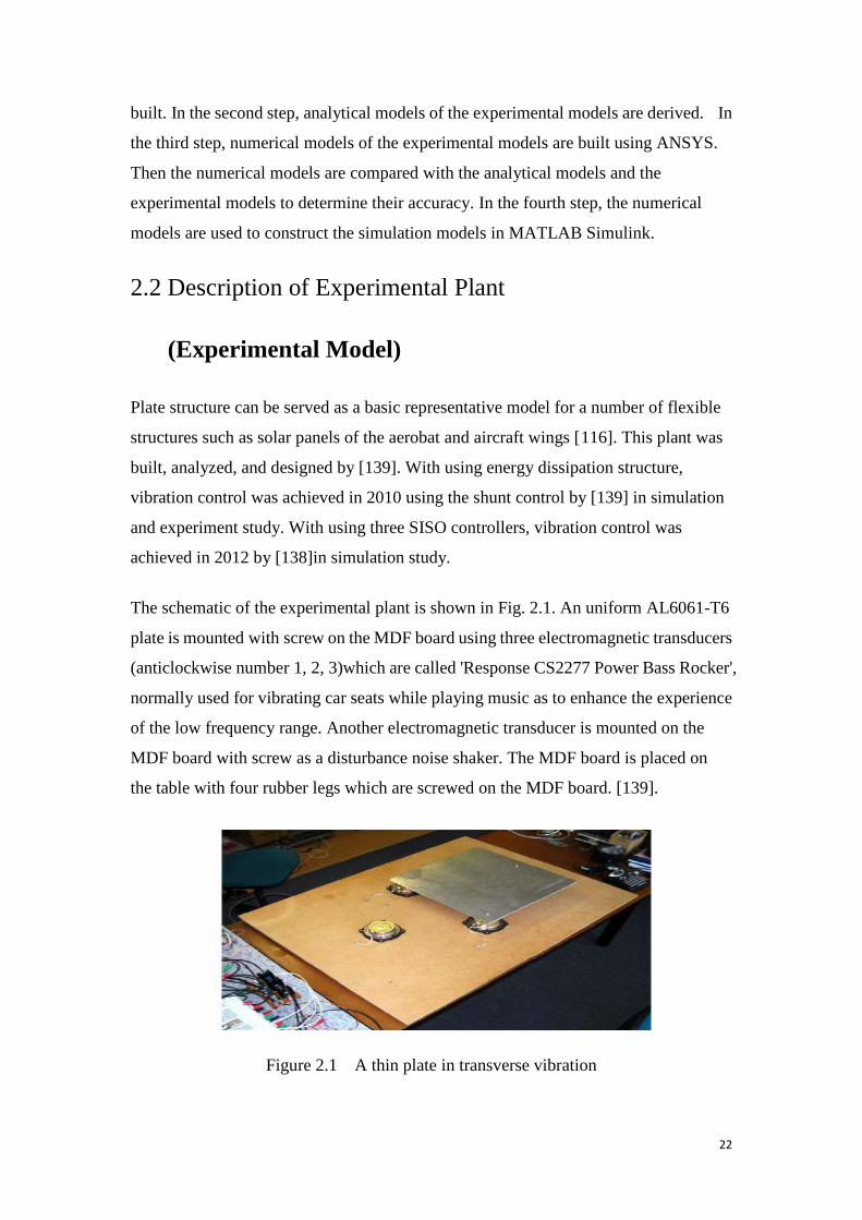
Plate structure can be served as a basic representative model for a number of flexible
structures such as solar panels of the aerobat and aircraft wings [116]. This plant was
built, analyzed, and designed by [139]. With using energy dissipation structure,
vibration control was achieved in 2010 using the shunt control by [139] in simulation
and experiment study. With using three SISO controllers, vibration control was
achieved in 2012 by [138]in simulation study.
The schematic of the experimental plant is shown in Fig. 2.1. An uniform AL6061-T6
plate is mounted with screw on the MDF board using three electromagnetic transducers
(anticlockwise number 1, 2, 3)which are called 'Response CS2277 Power Bass Rocker',
normally used for vibrating car seats while playing music as to enhance the experience
of the low frequency range. Another electromagnetic transducer is mounted on the
MDF board with screw as a disturbance noise shaker. The MDF board is placed on
the table with four rubber legs which are screwed on the MDF board. [139].
Figure 2.1 A thin plate in transverse vibration
23
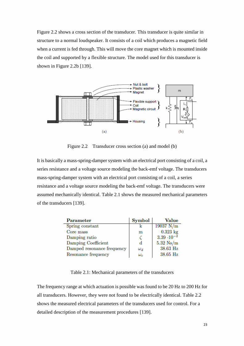
Figure 2.2 shows a cross section of the transducer. This transducer is quite similar in
structure to a normal loudspeaker. It consists of a coil which produces a magnetic field
when a current is fed through. This will move the core magnet which is mounted inside
the coil and supported by a flexible structure. The model used for this transducer is
shown in Figure 2.2b [139].
Figure 2.2 Transducer cross section (a) and model (b)
It is basically a mass-spring-damper system with an electrical port consisting of a coil, a
series resistance and a voltage source modeling the back-emf voltage. The transducers
mass-spring-damper system with an electrical port consisting of a coil, a series
resistance and a voltage source modeling the back-emf voltage. The transducers were
assumed mechanically identical. Table 2.1 shows the measured mechanical parameters
of the transducers [139].
Table 2.1: Mechanical parameters of the transducers
The frequency range at which actuation is possible was found to be 20 Hz to 200 Hz for
all transducers. However, they were not found to be electrically identical. Table 2.2
shows the measured electrical parameters of the transducers used for control. For a
detailed description of the measurement procedures [139].

24
As stated in 1.5.3 of Chapter 1, PPF combine with Genetic Algorithms (GA), the
optimal control position of the three control transducers can be derived through GA
calculation. The author did not derived that because the limited time, the other reason
is that during the implementation, for some mechanical plant systems, some optimal
positions may not be used due to the physical conditions. Expect the analytical GA
calculation, the other easier method is that set up the model and do the simulation
using the numerical software such as ANSYS. It is easier to find and confirm the
minimum displacement of the observation position according to different control
transducer position.
Parameter Symbol T 1 T 2 T 3
Impedance at 50 Hz Zi[Ω] 3.6170 3.7204 3.8442
Inductance at 50 Hz Li[µH] 518 533 597
Resistance at 50 Hz Ri[Ω] 3.6133 3.7166 3.8396
Current-Force coupling at 26.9 Hz CiF [N/A] 2.0523 3.6361 3.6996
Velocity-Voltage coupling at 26.9 Hz CυV [Vs/m] 2.0523 3.6361 3.6996
Table 2.2: Electrical parameters of the three transducers (T 1, 2 and 3)
The natural frequencies of the experimental models are the most important parameters
to be considered for the proposed control methods. Therefore, a series of experiments
are undertaken to measure the natural frequencies of the experimental model. The
natural frequencies are obtained by applying a sweep signal to experimental model. The
amplitude of the vibration is then measured against the frequency of the signal. The
frequencies where the amplitude of vibration forms a peak are the natural frequencies
of the experimental model. In the experiment, a sweep signal from a signal generator is
amplified by a 50 W Jay Car amplifier and the output from the amplifier is applied to
the disturbance noise transducer. The attenuation is necessary in order to make the
signal level suitable for input to the analog-to-digital converter. The amplitude of the
vibration is measured by accelerometers then it is shown on Agilent 54621A
oscilloscope. Experiments show that the dominant modes for all the experimental
models are the first four modes. The frequencies for the first four modes are shown in

25
Table 2.3 [139].
In the next section analytical models of the experimental model will be de rived.
Table 2.3: The first four natural frequencies of the experimental model
2.3 Numerical Solution Using ANSYS
(Numerical Model)
In practice, especially for complex structures, a software tool such as ANSYS can be
used to find the natural frequencies of the structures. ANSYS uses the finite-element
method (FEM) to solve the underlying governing equations and the associated
problem-specific boundary conditions. FEM tools are used widely in industry to
simulate the responses of a physical system to structural loading, and thermal and
electromagnetic effects. In this research, ANSYS software version 14.0 is used to find
the natural frequencies of the plate structure. The results are validated through
comparison with the results from the experimental and analytical method [4]. This
numerical model was built, analyzed, and designed by [139], and also studied by [138].
Due to the limitation of the transducers, the author adjusted the thickness of the top
plate and MDF board, and other relevant parts in the numerical model to make sure
that the first natural frequency of the top plate is within the frequency range of the
transducers.

26
Figure 2.3 System model shown in isometric view and side view
2.3.1 Resonance Frequency
Normal mode, an inherent property of the system, is characterized with a specific
natural frequency, damping ratio and mode shape, and it can be applied to describe the
system motion called resonance which is approximate equal to the natural
frequency[117,118,119]. For any system, modes are totally independent with each
other so that they have different modal parameters including natural
frequencies, damping ratios and mode shapes (even if the same value). Those modal
parameters normally depend on the system structure, materials and boundary
conditions. Hence, the excitation of one mode of a system would not cause the motion
of different mode. In ANSYS, the modal analysis module is able to be used for
computing the resonant frequencies and corresponding mode shapes [4].
Resonance frequency (or natural frequency) refers to a certain frequency that is able to
lead the significant magnitude of the oscillation. To determine the dynamics on the top
plate, start with modal analyses so that the resonance frequencies can be found.
In the simulation the model is supposed to be analyzed in range of [0, 200 Hz] due to
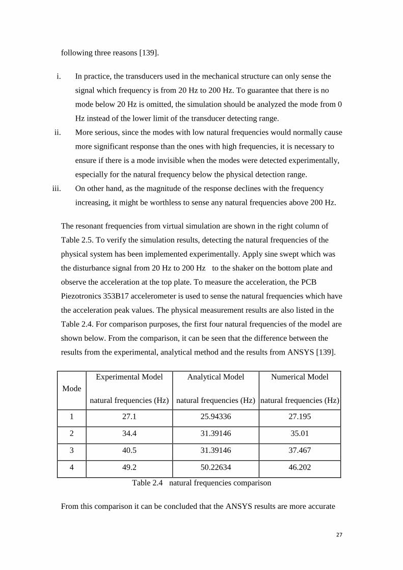
27
following three reasons [139].
i. In practice, the transducers used in the mechanical structure can only sense the
signal which frequency is from 20 Hz to 200 Hz. To guarantee that there is no
mode below 20 Hz is omitted, the simulation should be analyzed the mode from 0
Hz instead of the lower limit of the transducer detecting range.
ii. More serious, since the modes with low natural frequencies would normally cause
more significant response than the ones with high frequencies, it is necessary to
ensure if there is a mode invisible when the modes were detected experimentally,
especially for the natural frequency below the physical detection range.
iii. On other hand, as the magnitude of the response declines with the frequency
increasing, it might be worthless to sense any natural frequencies above 200 Hz.
The resonant frequencies from virtual simulation are shown in the right column of
Table 2.5. To verify the simulation results, detecting the natural frequencies of the
physical system has been implemented experimentally. Apply sine swept which was
the disturbance signal from 20 Hz to 200 Hz to the shaker on the bottom plate and
observe the acceleration at the top plate. To measure the acceleration, the PCB
Piezotronics 353B17 accelerometer is used to sense the natural frequencies which have
the acceleration peak values. The physical measurement results are also listed in the
Table 2.4. For comparison purposes, the first four natural frequencies of the model are
shown below. From the comparison, it can be seen that the difference between the
results from the experimental, analytical method and the results from ANSYS [139].
Mode Experimental Model
natural frequencies (Hz)
Analytical Model
natural frequencies (Hz)
Numerical Model
natural frequencies (Hz)
1 27.1 25.94336 27.195
2 34.4 31.39146 35.01
3 40.5 31.39146 37.467
4 49.2 50.22634 46.202
Table 2.4 natural frequencies comparison
From this comparison it can be concluded that the ANSYS results are more accurate

28
cause the deformation is more complex and the deformation equation which had been
derived from theoretical analysis can not exactly predict the deformation. Based on the
accuracy of the results, numerical model from ANSYS will be used here to form
simulation model for the experimental plant.
2.3.2 Mode Shape
Mode shape, one of the mode parameters, describes a deflection pattern associated with
a particular natural frequency. Same as the natural frequency, mode shape is
independent with the ones with other modes. The actual deformation or displacement at
arbitrary point of the structure is the summation of all the mode shapes of that
system[118,119]. Basically, the pure mode shapes can be generated and observed as the
displacement if the external harmonic excitations have the same frequencies as the
system modes. Conversely, the excitations with random frequencies tend to produce an
arbitrary “shuffling” of all the structural mode shapes superposition. The mode shape
can be treated as the inherent dynamic property when the system is in free vibration
without any external force applying. In another word, the mode shapes can be
considered as the superposed deflection of the all parts in the system [139].
Figure 2.4 Modal Analysis mode shape of first mode

29
Figure 2.5 Modal Analysis mode shape of second mode
Figure 2.6 Modal Analysis mode shape of third mode
Figure 2.7 Modal Analysis mode shape of forth mode

30
In ANSYS, the mode shapes can be obtained by implementing the modal analysis such
as Fig 2.4−2.7. With the given mode which has been determined before, the modal
shape is computed and represented as maximum deformation or displacement.
2.3.3 Harmonic Response Analysis
Instead of computing the transient vibrations which exists at the beginnings the
excitation, the ANSYS harmonic response analysis technique calculates the steady –
state response of the linear structure system to loads that vary harmonically [118,119].
That is, harmonic analysis can be applied with given (range of) frequency (frequencies)
when the structure is in forced vibration. In the harmonic analysis, once the input has
been determined, the corresponding output could be computed. Note that the dynamic
between input and output which is characterized by natural frequency, damping ratio
and mode shape, is the inherent property of the existed system. It means that the system
dynamic would not change whatever the external excitation is applied unless the
system itself has been changed. To determine the dynamic between shaker and any
positions on the top plate, apply 1N force through the shaker and collect the results
given as deflections from the top plate. For instance, as shown in Figure 2.8, the 1N
force, which is the user-defined input, has been applied to the shaker with specific
natural frequency. The amplitude and phase response result of the whole top plate is
shown in Figure 2.9 and 2.10. The harmonic analysis is also able to present the
corresponding deflections at the position of each transducer. The same implementation
can be applied to the shaker, while other three transducers (transducer 1, 2, 3 and the
shaker) are considered as outputs [139].
Figure 2.8 Harmonic Analysis Example

31
With applying 1N force via the shaker (input), respectively, the corresponding
deflection of transducer in millimetre (output) only depends on that single input and its
related dynamic. The harmonic analysis results is shown at Figure 2.11.
It is shown that for Fig 2.11(a), at transducer 1, the mode shape of mode 2 and 4 are
very small. For Fig 2.11 (b) and (c), only three modes can be seen because the mode
shape of mode 2 is very small
Figure 2.9 Amplitude Response of whole top plate to a harmonic disturbance at shaker
Figure 2.10 Phase Response of whole top plate to a harmonic disturbance at shaker

32
(a) Transducer 1 resonant peaks
(b) Transducer 1 resonance phase

33
(c) Transducer 2 resonance peaks
(d) Transducer 2 resonance phase

34
(e) Transducer 3 resonance peaks
(f) Transducer 3 resonance phase
Figure 2.11 Simulated harmonic disturbance at shaker and measured resonant peaks and phase of top plate at transducer 1 (a, b), transducer 2 (c, d) and transducer 3 (e, f).
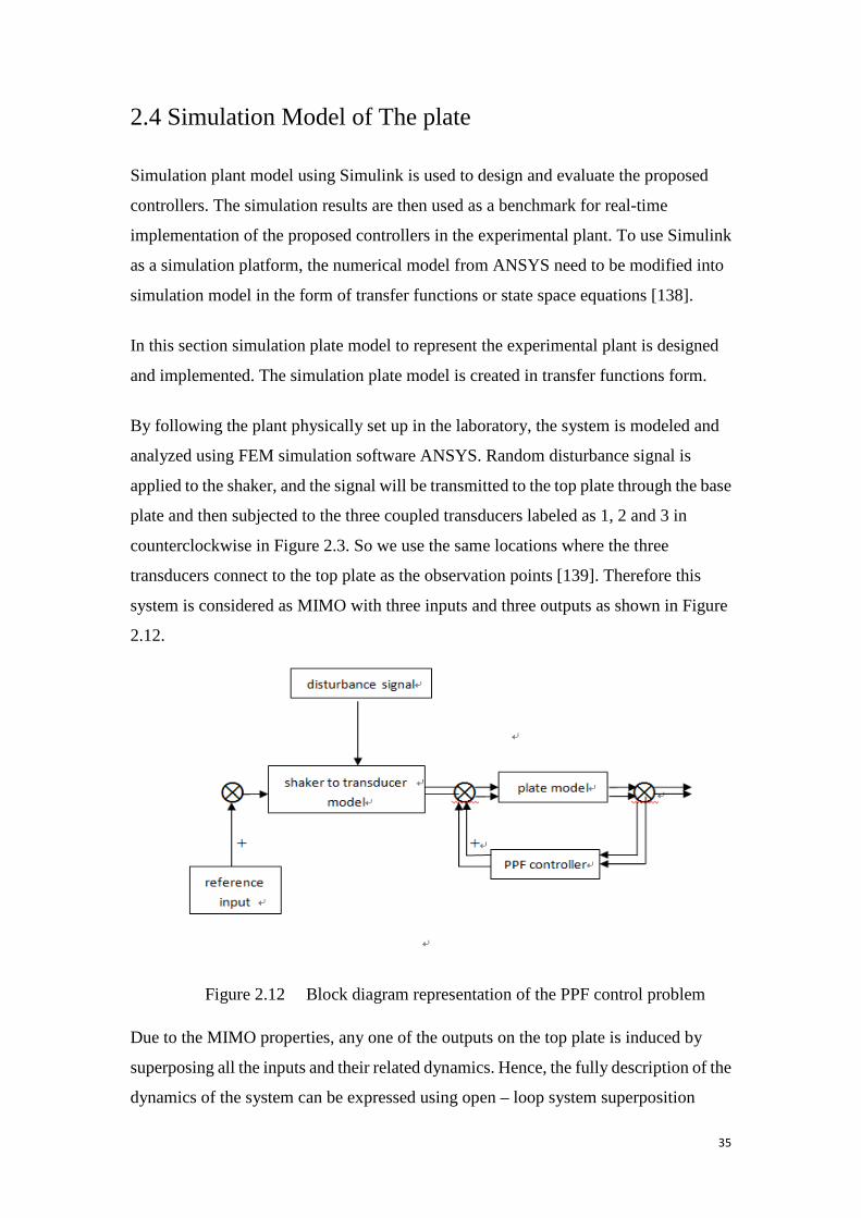
35
2.4 Simulation Model of The plate
Simulation plant model using Simulink is used to design and evaluate the proposed
controllers. The simulation results are then used as a benchmark for real-time
implementation of the proposed controllers in the experimental plant. To use Simulink
as a simulation platform, the numerical model from ANSYS need to be modified into
simulation model in the form of transfer functions or state space equations [138].
In this section simulation plate model to represent the experimental plant is designed
and implemented. The simulation plate model is created in transfer functions form.
By following the plant physically set up in the laboratory, the system is modeled and
analyzed using FEM simulation software ANSYS. Random disturbance signal is
applied to the shaker, and the signal will be transmitted to the top plate through the base
plate and then subjected to the three coupled transducers labeled as 1, 2 and 3 in
counterclockwise in Figure 2.3. So we use the same locations where the three
transducers connect to the top plate as the observation points [139]. Therefore this
system is considered as MIMO with three inputs and three outputs as shown in Figure
2.12.
Figure 2.12 Block diagram representation of the PPF control problem
Due to the MIMO properties, any one of the outputs on the top plate is induced by
superposing all the inputs and their related dynamics. Hence, the fully description of the
dynamics of the system can be expressed using open – loop system superposition

36
technology.
Y1(s)=Y11(s) + Y12(s) + Y13(s) + Y1d(s) = T11(s) U1(s) + T12(s) U2(s) + T13(s) U3(s)
(2.1a)
Y2(s)=Y21(s) + Y22(s) + Y23(s) + Y2d(s) = T21(s) U1(s) + T22(s) U2(s) + T23(s) U3(s)
(2.1b)
Y3(s)=Y31(s) + Y32(s) + Y33(s) + Y3d(s) = T31(s) U1(s) + T32(s) U2(s) + T33(s) U3(s)
(2.1c)
The equations (2.130a-2.130c) can be illustrated using matrix form
Y1(s)Y2(s)Y3(s)
= T11(s) T12(s)T21(s) T22(s)
T13(s)T23(s)
T31(s) T32(s) T33(s) *
U1(s)U2(s)U3(s)
(2.2)
where
U1(s)U2(s)U3(s)
= D1(s)D2(s)D3(s)
* Ud(s) (2.3)
Ui - input through the transducer i to the top plate, i = 1, 2, 3
Ud - input to shaker
Yi - output at the position on the top plate, i = 1, 2, 3
Di - dynamic between the shaker and transducer
Tmn - dynamic between transducer m and n, m = 1, 2, 3, n = 1, 2, 3
When the three transducers are treated as three SISO system, the only difference is
that only the diagonal elements exist, other elements are equal to zero.
Based all the information before, we could set up the simulation model of the plate

37
plant in MATLAB, the model include SISO model and MIMO model.
Due to fact that there is no available spectrum analyzer in the laboratory and
workshop, no budget to buy or rent the equipment, we could not plot the numerical
result and compare with the experimental result, according to [120], we hope that we
can adopt 150 modes plate model as the simulation model, and compare the truncated
model which used balanced truncation method with the 150 modes simulation model.
When simulation model was calculated by the MATLAB software, we found that if
there is more than 47 modes in the plate model, the parameter in the denominator
would be too small that MATLAB could not recognize and treat it as infinite small.
So what we can do is that we adopt 47 modes in the plate model and take it as the
simulation model.
SISO 47 modes plate model is shown in Figure 2.13-2.16. MIMO 47 modes plate
model is shown in Figure 2.17-2.26.
Figure 2.13 three SISO (g11,g22,g33) 47 modes plate model

38
Figure 2.14 SISO (g11) 47 modes plate model at transducer 1
Figure 2.15 SISO (g22) 47 modes plate model at transducer 2
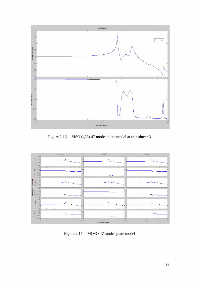
39
Figure 2.16 SISO (g33) 47 modes plate model at transducer 3
Figure 2.17 MIMO 47 modes plate model

40
Figure 2.18 MIMO (Gp(1,1)) 47 modes plate model
Figure 2.19 MIMO (Gp(1,2)) 47 modes plate model

41
Figure 2.20 MIMO (Gp(1,3)) 47 modes plate model
Figure 2.21 MIMO (Gp(2,1)) 47 modes plate model
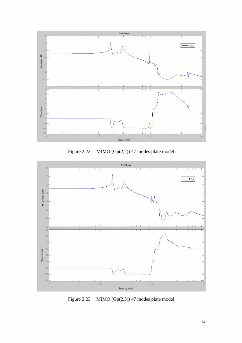
42
Figure 2.22 MIMO (Gp(2,2)) 47 modes plate model
Figure 2.23 MIMO (Gp(2,3)) 47 modes plate model

43
Figure 2.24 MIMO (Gp(3,1)) 47 modes plate model
Figure 2.25 MIMO (Gp(3,2)) 47 modes plate model
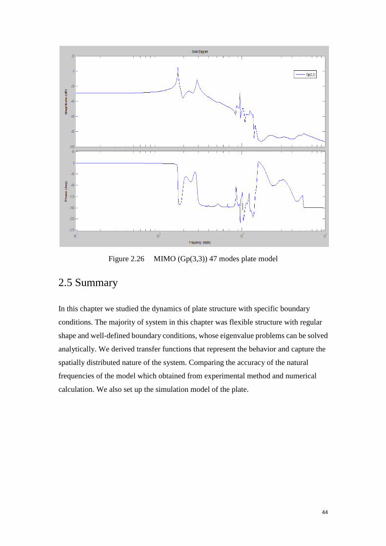
44
Figure 2.26 MIMO (Gp(3,3)) 47 modes plate model
2.5 Summary
In this chapter we studied the dynamics of plate structure with specific boundary
conditions. The majority of system in this chapter was flexible structure with regular
shape and well-defined boundary conditions, whose eigenvalue problems can be solved
analytically. We derived transfer functions that represent the behavior and capture the
spatially distributed nature of the system. Comparing the accuracy of the natural
frequencies of the model which obtained from experimental method and numerical
calculation. We also set up the simulation model of the plate.
45
Chapter 3
Spatial Norm and Model Reduction
3.1 Introduction
Modeling of physical systems often results in high order models. It is desirable to
reduce such a high-order model to a simpler model of lower dimension. The problem of
model reduction is important since the majority of modern controller design techniques
(such as H∞ and LQG design methods) result in a controller of dimension equal to that
of the plant. Hence, a controller design based on a suitable reduced model would result
in a lower order controller which would reduce implementation problems [113]. In
order to use the model in analysis and synthesis problems, we need to define suitable
performance measures that take into account their spatially distributed nature.
Traditional performance measures, such as H2 and H∞ norms, only deal with
point-wise models for such systems. In this chapter, we extend these performance
measures to include the spatial characteristics of spatially distributed systems [113].
Another topic that is covered in this chapter is that of model reduction by balanced
truncation. The problem of model reduction for dynamical systems has been studied
extensively throughout the literature; see, for example, [121,122] Here, we address the
problem for spatially distributed linear time-invariant systems, following [123].
3.2 Plate Model Reduction and Balanced Realization
3.2.1 SISO Plate Model Reduction and Balanced Realization
Based on the knowledge in [113], we can use spatial H2 and H∞norm for spatially
distributed systems. This norm can be used as measures of performance in certain
analysis and synthesis problems. In some cases, it can be beneficial to add a spatial
weighting function to emphasize certain regions [113]. In this section, we extend those
definitions to allow for spatially distributed weighting functions. So we can reduce the

46
plate model order by the balanced method: Fig 3.1-3.8 are shown the SISO plate
model reduction by balanced truncation method.
Figure 3.1 SISO Plate (g11) at transducer 1 Hankel singular values
Figure 3.2 SISO Plate (g11) at transducer 1 model reduction and balanced
realization frequency domain compare

47
Figure 3.3 SISO Plate (g11) at transducer 1 model reduction and balanced
realization singular values compare
Figure 3.4 SISO Plate (g22) at transducer 2 Hankel singular values

48
Figure 3.5 SISO Plate (g22) at transducer 2 model reduction and balanced
realization frequency domain compare
Figure 3.6 SISO Plate (g22) at transducer 2 model reduction and balanced
realization singular values compare

49
Figure 3.7 SISO Plate (g33) at transducer 3 Hankel singular values
Figure 3.8 SISO Plate (g33) at transducer 3 model reduction and balanced
realization frequency domain compare

50
Figure 3.9 SISO Plate (g33) at transducer 3 model reduction and balanced
Realization singular values compare
We can see that, according to Hankel singular values, first 44 states of g11, first 36
states of g22, first 32 states of g33 are all unstable states, so if we want to reduce the
order of the model, we need to obtain all the unstable states. It can be seen that the
"balreal" method is better compare to others.
3.2.2 MIMO Plate Model Balanced truncation
Fig 3.10-3.12 are shown the MIMO plate model reduction by balanced truncation
method.
Figure 3.10 MIMO Plate Hankel singular values

51
Figure 3.11 MIMO Plate model reduction and balanced realization frequency
domain compare
Figure 3.12 MIMO Plate model reduction and balanced realization singular values
compare
It can be seen that the "balreal" method is better compare to others.

52
3.3 Summary
In this chapter, we showed the method to reduce the model order by balanced
truncation method, and also introduce the spatial norm of model. We gave the
performance of "balred", "balreal" and "modred" for SISO plate model, the
performance of "balred" and "balreal" and for MIMO plate model, and according to
compare the performance, we gave the decision that "balreal" balanced truncation
method is better both for SISO and MIMO plate model, but for some cases caused too
big phase angle.
53
Chapter 4
Model Correction
4.1 Introduction
Dynamics of flexible structures and some acoustic systems consist of an infinite
number of modes. For control design purposes these models are often approximated by
finite-dimensional models via truncation. Direct truncation of higher order modes
results in the perturbation of zero dynamics and hence generates errors in the spatial
frequency response of the system. If the truncated model is then used to design a
controller which is implemented on the system, say in the laboratory, the closed loop
performance of the system can be considerably different from the theoretical
predictions. This is mainly due to the fact that although the poles of the truncated
system are at the correct frequencies, the zeros can be far away from where they should
be. Therefore, it is natural to expect that a controller designed for the truncated [113].
Reference [124] discusses the effect of out of bandwidth modes on the low-frequency
zeros of the truncated model. There, it is suggested that the effect of higher frequency
modes on the low frequency dynamics of the system can be captured by adding a zero
frequency term to the truncated model to account for the compliance of the ignored
modes [133]. The model correction method that is proposed allows for a spatially
distributed DC term to capture the effect of truncated modes in an optimal way. In this
chapter, we take a similar approach in the sense that we allow for a zero frequency term
to capture the effect of truncated modes. However, this constant term is found such that
the H2 norm of the resulting error system is minimized [113].
4.2 Plate Correction Model
As discussed in Chapter 3, Fig 3.1, 3.4, 3.7, 3.10 showed that there are unstable states
in the Hankel singular values, so we could not choose the state which we want to save
and truncate as normal, so we just focus on the first four modes in this study.
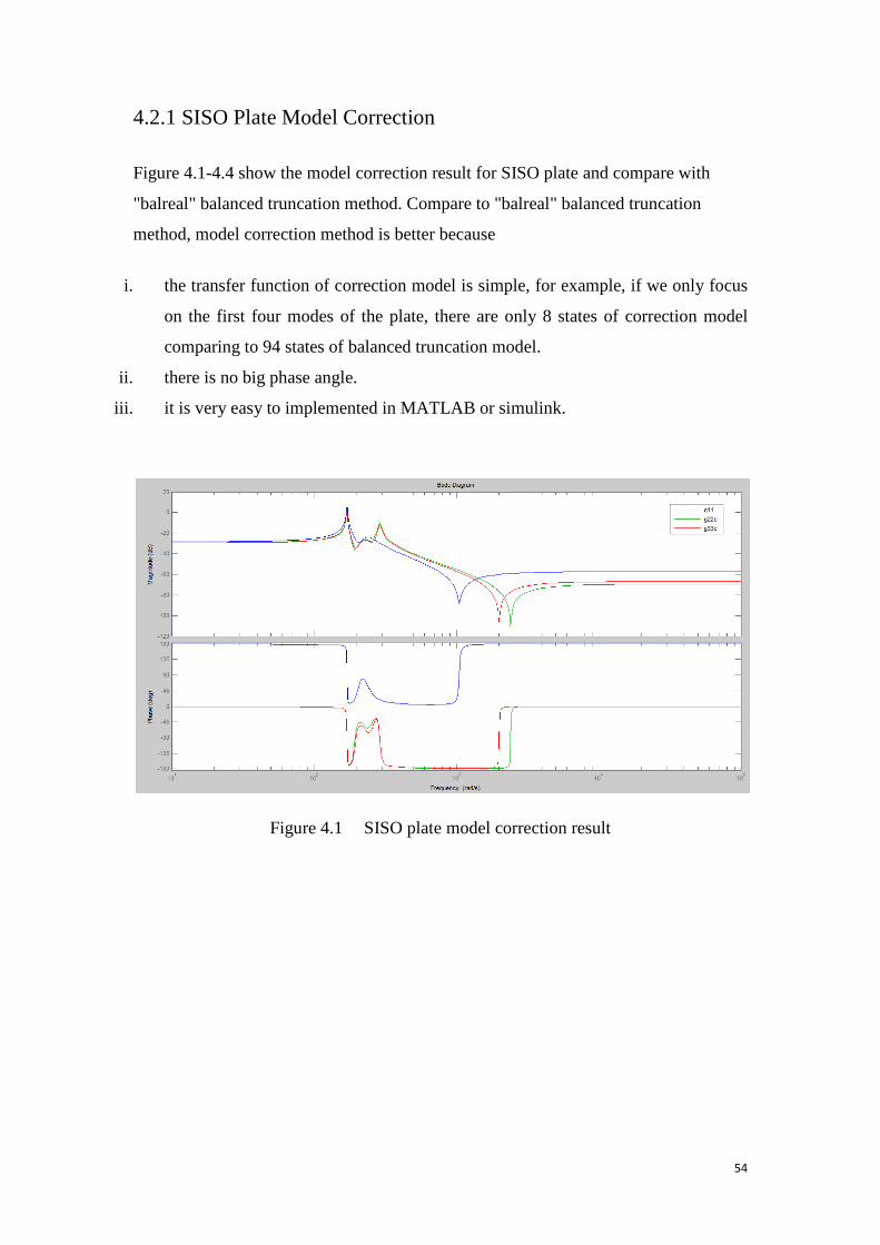
54
4.2.1 SISO Plate Model Correction
Figure 4.1-4.4 show the model correction result for SISO plate and compare with
"balreal" balanced truncation method. Compare to "balreal" balanced truncation
method, model correction method is better because
i. the transfer function of correction model is simple, for example, if we only focus
on the first four modes of the plate, there are only 8 states of correction model
comparing to 94 states of balanced truncation model.
ii. there is no big phase angle.
iii. it is very easy to implemented in MATLAB or simulink.
Figure 4.1 SISO plate model correction result

55
Figure 4.2 SISO plate (g11) model reduction result compare (balreal and correction)
Figure 4.3 SISO plate (g22) model reduction result compare (balreal and correction)

56
Figure 4.4 SISO plate (g33) model reduction result compare (balreal and correction)
4.2.2 MIMO Plate Model Correction
Figure 4.5 MIMO plate model reduction result compare (balreal and correction)

57
Figure 4.6 MIMO Plate model correction and balanced truncation singular values
compare
Figure 4.7 MIMO (Gpc(1,1)) plate model correction result

58
Figure 4.8 MIMO (Gpc(1,2)) plate model correction result
Figure 4.9 MIMO (Gpc(1,3)) plate model correction result

59
Figure 4.10 MIMO (Gpc(2,1)) plate model correction result
Figure 4.11 MIMO (Gpc(2,2)) plate model correction result

60
Figure 4.12 MIMO (Gpc(2,3)) plate model correction result
Figure 4.13 MIMO (Gpc(3,1)) plate model correction result

61
Figure 4.14 MIMO (Gpc(3,2)) plate model correction result
Figure 4.15 MIMO (Gpc(3,3)) plate model correction result

62
4.3 Summary
In this chapter, we reported the method to truncate the model order by correction
method. We gave the performance of "balreal" balanced truncation and model
correction for SISO and MIMO plate model. According to compare the performance,
we made the decision that model correction method is better both for SISO and
MIMO plate model.

63
Chapter 5
Multi-mode SISO and MIMO PPF
Controller
This chapter provides an overview of the positive position feedback (PPF) technique.
In the first two section general information and structure about PPF is given. The third
section shows the PPF controller stability derivation. This derivation itself is not
original and can also be found in [125,1,3]. The following section shows the selection
method of the optimal controller parameters and MATLAB simulation result.
5.1 Introduction
As shown in Chapter 2, one of the characteristics of flexible structures is their highly
resonant nature. For the case of the plate used in this research this characteristic is
made evident by the relatively large vibration at or near to the natural frequencies of
the structure, as shown in Fig. 2.5. From the figure, it is clear that suppressing the
vibration of a structure at or very close to the natural frequencies of the structure is
more important than suppressing the vibration at other frequencies. However,
suppressing the vibration at one or more natural frequencies may excite or amplify
other natural frequencies. Therefore, one important design requirement for flexible
structure control is to achieve high attenuation for modes of interest without driving
the other modes into instability or exciting and amplifying the vibration of other
modes [4].
As stated in Chapter 1, a resonant PPF controller has necessary characteristics that
satisfy the design requirements for multi-mode vibration attenuation of flexible
structures investigated in this research. Exploiting the highly resonant characteristic of
the flexible structure, the resonant PPF controller only applies high gain at or close to
the natural frequencies of interest, and is therefore able to suppress the vibration at
those frequencies without causing adverse effects at other frequencies. In the
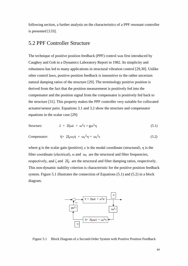
64
following section, a further analysis on the characteristics of a PPF resonant controller
is presented [133].
5.2 PPF Controller Structure
The technique of positive position feedback (PPF) control was first introduced by
Caughey and Goh in a Dynamics Laboratory Report in 1982. Its simplicity and
robustness has led to many applications in structural vibration control [29,30]. Unlike
other control laws, positive position feedback is insensitive to the rather uncertain
natural damping ratios of the structure [29]. The terminology positive position is
derived from the fact that the position measurement is positively fed into the
compensator and the position signal from the compensator is positively fed back to
the structure [31]. This property makes the PPF controller very suitable for collocated
actuator/sensor pairs. Equations 3.1 and 3.2 show the structure and compensator
equations in the scalar case [29]:
Structure: ε + 2ξωε + ω2ε = gω2η (5.1)
Compensator: η+ 2ξfωfη + ωf2η = ωf
2ε (5.2)
where g is the scalar gain (positive), ε is the modal coordinate (structural), η is the
filter coordinate (electrical), ω and ωf are the structural and filter frequencies,
respectively, and ζ and 2ξf are the structural and filter damping ratios, respectively.
This non-dynamic stability criterion is characteristic for the positive position feedback
system. Figure 5.1 illustrates the connection of Equations (5.1) and (5.2) in a block
diagram.
Figure 5.1 Block Diagram of a Second-Order System with Positive Position Feedback

65
The second-order transfer function in Equation (5.3) also represents the PPF
compensator. The transfer function form will be used in this text for deriving the
properties of the control system [29].
Gppf (s) = gωf2
s2+ 2ξfωfs+ ωf2 (5.3)
Another feature of the compensator equation, its second-order low-pass characteristic,
led to the terminology PPF filter. Figure 5.3 presents a Bode plot of a typical PPF
filter. In effect, a PPF filter behaves much like an electronic vibration absorber for the
structure except that a mechanical vibration absorber can never destabilize a
structure[133,124].
Figure 5.2 Bode Plot of a Typical PPF Filter Frequency Response Function
The roll-off character of the PPF filter is one of the advantages of using a PPF
controller. Structural poles with frequencies higher than the filter frequencies are
hardly affected by the compensator. This is especially useful when complicated
structures with many resonance poles are to be controlled. PPF is able to add damping
to lower frequency poles while leaving the possibly unmodeled high frequency poles
unchanged [133,124].
Since one PPF filter tuned to a certain frequency only adds damping to one certain
pole of the structure, the possibilities of multiple PPF were investigated by many
authors [28]. Multiple PPF filters allow that each filter is tuned to add damping to one
structural pole while only using one actuator/sensor pair.

66
Unfortunately, the stability criterion is not as simple as for the one PPF filter case but
experiments have shown that for widely spaced poles with up to three PPF filters the
stability is usually not a problem [29].
5.3 PPF Controller Closed -loop Stability
5.3.1 Scalar Case
Considering the scalar case first, PPF can be described by two coupled differential
equations where the first equation describes structure, and the second describes the
compensator as[29]
ε+βε+ω2ε=gω2η (5.4)
η+βfη+ωf2η=ωf
2ε (5.5)
where ε is the system coordinate, η is the actuator coordinate, ε,η ∈R, β and βf are the system
damping and actuator damping ratios, ω and ωf are the structural natural frequency and filter
frequency, and g is the scalar gain, g > 0.
Theorem 5.1
The combined system and actuator of (5.4) and (5.5) are Liapunov asymptotic stable iff g < 1.
(Also serves as the stability boundary.)
Proof :
Taking the Laplace transform of the second-order equation (5.4) and (5.5)
(s2+ βs+ω2)⋅ ε(s)=gω2⋅ η (s) (5.6)
(s2+ βfs+ωf2)⋅ η (s)=ωf
2⋅ ε (s) (5.7)
So we can get
ε(s)η (s)
= gω2
s2+ βs+ω2=s2+ βfs+ω f2
ω f 2 (5.8)

67
The closed loop characteristic equation for (1) and (2) is
(s2 + βs + ω2) ⋅ (s2+ βfs+ωf2) - gω2ωf
2 = 0 (5.9)
Then we can achieve
s4+(β + βf) s3+(ω2 + ωf2 + β βf) s2+(βfω
2 + βωf2) s
+ (1 − g) ω2ωf2 = 0 (5.10)
A sufficient and necessary condition for stability is that all the principal minors of the
corresponding Routh - Hurwitz array be greater than zero. The principal minors of (7) can be
easily show to be
s4: 1 ω2 + ωf2 + β βf (1- g) ω2ωf
2
s3: β + βf βfω2 + βωf
2 0
s2: β+βf∗ω2+ω f
2+β βf−(βfω2+βωf
2)β+βf
(1- g) ∗ ω2 ∗ ωf2 0
s1: βω2+βfω f
2+ββfβ+βf∗βfω2+βωf
2−(β+βf)2∗(1− g) ∗ω2∗ ω f
2
βω2+βfω f 2+ββf(β+βf) 0
s0: (1- g) ∗ ω2 ∗ ωf2
M1 = β + βf (5.11)
M2 = βω2 + βfωf2 + ββf(β + βf) (5.12)
M3 = ββf ω2 −ωf
22 + β + βfβωf
2 + βfω2 + g(β + βf)
2ω2ωf2 (5.13)
M4 = (1- g) ∗ ω2 ∗ ωf2 (5.14)
Thus for positive g, M1, M2, & 𝑀𝑀3 are unconditionally positive. M4 is positive iff g < 1, and
the proof is complete.

68
5.3.2 Multivariate Case
Having understood the scalar system, the idea of position feedback can be easily generalized
into the multivariate system. The equations governing position feedback (collocated actuators
and sensors) control of a quasi-distributer parameter system with actuator dynamics are given
by[1,133,124]
M y + D y + K y = STC u (5.15)
u + βа u + ωа2(u− S y) = 0 (5.16)
where y ∈ ℝN is the system state vector and u ∈ ℝNA the actuator state vector. The
NAxNA gain matrix C is positive definite and can be factorized, using its square root C12 as
follows:
CT2 C1
2 = C (5.17)
The modal form of the system is obtained by applying the following transformation
y = ϕξ (5.18)
η = 1ωа
C12 u (5.19)
so that
ξ + Dξ + Ωξ = ωаϕTSTCT2 η (5.20)
η + βаη + ωа2η = ωаC1
2 S ϕξ (5.21)
or
ξ η + D 00 βаINA
ξη + Ω −ωаϕTSTCT
2
−ωаC12 S ωа
2INA
ξη = 0 (5.22)
Theorem 5.2
The combined system and actuator dynamics as represented by (5.19) are Liapunov
asymptotic stable if

69
Ω − (1+ ε) B is positive definite (5.23)
where ε is some arbitrarily small positive quantity and B is the modal gain matrix given by
B = ϕTSTCS ϕ (5.24)
Theorem 5.3
For a second order multivariate dynamical system described by
IZ+𝒬𝒬Z+𝒫𝒫Z = 0 (5.25)
where Z, 𝒬𝒬, 𝒫𝒫 are of appropriate dimension and 𝒬𝒬 is positive definite, a sufficient and
necessary condition for Liapunov asymptotic stability is that
𝒫𝒫 is positive definite (5.26)
Theorem 5.4
The system in (5.19) is LAS iff the modiffied stiffenss matrix
P = Ω −ωаϕTSTCT
2
−ωаC12 S ϕ ωа
2INA
is positive definite (5.27)
Note that the sufficient condition for stability (5.20) is equivalent to
K − (1 + ε) STCS is positive definite
5.3.3 Multivariate PPF Controller implemented with feed-through plant
Based on Chapter 4, addition of feed-through term to the truncated model is quite important,
if the truncation is not to substantially alter open-loop zeros of the system. Although the
truncation does not perturb open-loop poles of the system, it has the potential to significantly
move the open-loop zeros, particularly when the actuators and sensors are collocated.
Consequently, if a feedback controller is designed for the truncated model, and then
implemented on the real system, the performance and stability of the closed loop system
could be adversely affected [1].
Normally PPF techniques which we talked before do not allow for a feed-through term in the
plant model. However, it is essential to include this in the design phase, if the implemented

70
controller is to perform in a satisfactory manner. Closed-loop performance of a controlled
system is highly dependent on open-loop zeros of the plant. Inclusion of a feed-through term
in the model ensures that closed-loop performance of the controller, once implemented, is in
close agreement with theoretical predictions [3]. The derivation below are from [1,133,124].
If we are concerned with designing high-performance feedback controllers for multivariable
resonant systems of the form
G(s)= ∑ ψ iψ i ′
s2+ 2ξiωi s + ωi2
Mi=1 (5.28)
where ψi is an mx1 vector, and M → ∞. In practice, however, the integer is finite, but
possibly a very large number which represents the number of modes that sufficiently describe
the elastic properties of the structure under excitation
Figure 5.3 Feedback control system associated with a flexible structure with
collocated actuator/sensor pairs, and subject to disturbance w
For a system of the form (5.41), a positive position feedback controller is defined as
Kpp (s) = ∑ −γ iγ i ′
s2+ 2δiω i s + ω i2
Ni=1 (5.29)
where γi ∈ ℝmx1 for i = 1, 2, ..., N.
where γi ∈ Rmx1 for i = 1, 2, ..., N
As illustrated in Fig. 5.3, due to the existence of the negative sign in all terms of (5.35), the
overall system resembles a positive feedback loop. Also, the transfer function matrix (5.34) is
71
similar to that of the force to displacement transfer function matrix associated with a flexible
structure, hence, the terminology positive position feedback.
An important property of PPF controllers is that to suppress one vibration mode requires only
one second-order term, as articulated in (5.35). Consequently, one can choose the modes,
within a specific bandwidth, that are to be controlled and construct the necessary controller.
To derive stability conditions for this control loop, the series in (5.36) is first truncated by
keeping the first N modes(N < M) that lie within the bandwidth of interest, and then
incorporating the effect of truncated modes by adding a feed-through term to the truncated
model. That is, to approximate (5.35) by
GN (s)= ∑ ψ iψ i ′
s2+ 2ξiω i s + ωi2
Ni=1 + D (5.30)
To derive stability of (5.43) under (5.42), the following theorem is needed.
Theorem 5.5: Consider the following second-order multivariable dynamical system:
x(t) + D x(t) + K x(t)= 0 (5.31)
where D, K ∈ RNxN and x ∈ RNx 1. Furthermore, assume that D = D' > 0. Then (5.37) is
exponentially stable if and only if K = K' > 0. Proof same as Theorem 5.3.
The following theorem gives the necessary and sufficient conditions for closed-loop stability
under positive position feedback. First, we need to make the following definitions:
Z =
⎣⎢⎢⎡ξ1
ξ2⋱
ξN⎦⎥⎥⎤ Ω =
⎣⎢⎢⎡ω1
ω2⋱
ωN⎦⎥⎥⎤
Ψ = [ψ1 ψ2 … ψN ]
and
∆ =
⎣⎢⎢⎡δ1
δ2⋱
δN ⎦⎥⎥⎤ Ω =
⎣⎢⎢⎡ω1
ω2⋱
ωN ⎦⎥⎥⎤
Γ = [γ1 γ2 … γN ]

72
Furthermore, we assume that
∆ > 0 (5.32)
Theorem 5.6: The negative feedback connection of (5.43) and (5.42) with (5.45) is
exponentially stable if and only if
Ω2− Γ'DΓ > 0 (5.33)
and
Ω2−Ψ'Γ(Ω2 − Γ′DΓ)−1Γ′Ψ > 0 (5.34)
5.4 Multi-mode SISO and MIMO PPF Controller Parameter
Selection
5.4.1 MATLAB Optimization toolbox and GA Optimization Search
In order to find the minimum value of H∞ norm, we need to use MATLAB Optimization
Toolbox, which provides widely used algorithms for standard and large-scale optimization.
These algorithms solve constrained and unconstrained continuous and discrete problems. The
toolbox includes functions for linear programming, quadratic programming, binary integer
programming, nonlinear optimization, nonlinear least squares, systems of nonlinear equations,
and multi-objective optimization. We can use them to find optimal solutions, perform tradeoff
analyses, balance multiple design alternatives, and incorporate optimization methods into
algorithms and models [140].
Key Features[140]:
i. Interactive tools for defining and solving optimization problems and monitoring solution
progress
ii. Solvers for nonlinear and multi-objective optimization
iii. Solvers for nonlinear least squares, data fitting, and nonlinear equations
iv. Methods for solving quadratic and linear programming problems
v. Methods for solving binary integer programming problems
In the toolbox, it contains several functions, such as GlobalSearch, MultiStart, Genetic
Algorithm, Direct Search, Simulated Annealing. For Genetic Algorithm, it is a method for

73
solving both constrained and unconstrained optimization problems that is based on natural
selection, the process that drives biological evolution. The genetic algorithm repeatedly
modifies a population of individual solutions. At each step, the genetic algorithm selects
individuals at random from the current population to be parents and uses them to produce the
children for the next generation. Over successive generations, the population "evolves"
toward an optimal solution. Genetic algorithm can be applied to solve a variety of
optimization problems that are not well suited for standard optimization algorithms, including
problems in which the objective function is discontinuous, nondifferentiable, stochastic, or
highly nonlinear. The genetic algorithm can address problems of mixed integer programming,
where some components are restricted to be integer-valued [140].
The genetic algorithm uses three main types of rules at each step to create the next generation
from the current population [140]:
i. Selection rules select the individuals, called parents, that contribute to the population at
the next generation.
ii. Crossover rules combine two parents to form children for the next generation.
iii. Mutation rules apply random changes to individual parents to form children
The genetic algorithm differs from a classical, derivative-based, optimization algorithm in
two main ways in the following table 5.1 [140]:
Classical Algorithm Genetic Algorithm
Generates a single point at each iteration.
The sequence of points approaches an
optimal solution.
Generates a population of points at each
iteration. The best point in the population
approaches an optimal solution.
Selects the next point in the sequence by a
deterministic computation.
Selects the next population by computation
which uses random number generators.
Table 5.1 classical algorithm and genetic algorithm comparison
Because the limited space, more details about Genetic Algorithm optimization toolbox please
refer to MATLAB user guide.
5.4.2 Multi-mode SISO PPF Controller Optimal Parameter Selection
Based the dynamics model between shaker and plate, the results of multi-mode SISO PPF
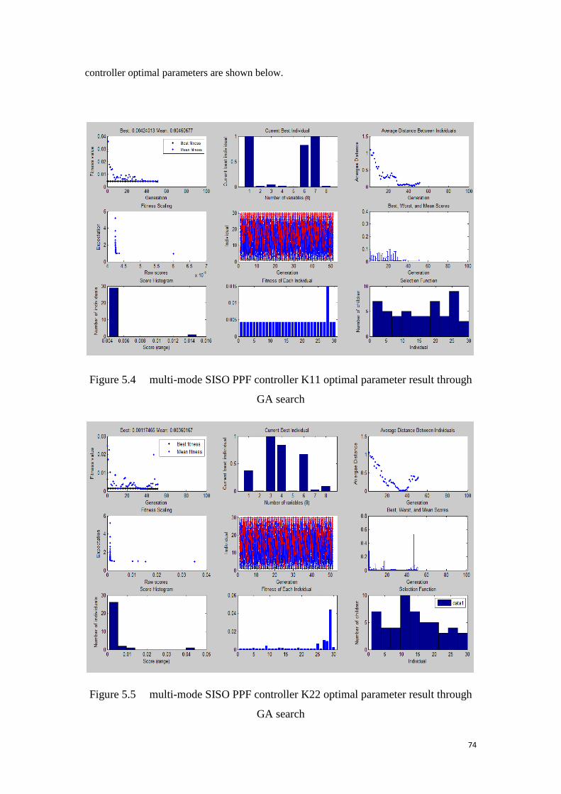
74
controller optimal parameters are shown below.
Figure 5.4 multi-mode SISO PPF controller K11 optimal parameter result through
GA search
Figure 5.5 multi-mode SISO PPF controller K22 optimal parameter result through
GA search
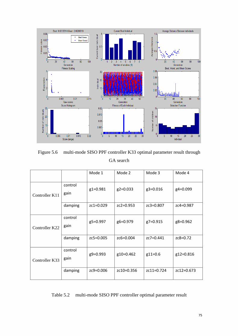
75
Figure 5.6 multi-mode SISO PPF controller K33 optimal parameter result through
GA search
Mode 1 Mode 2 Mode 3 Mode 4
Controller K11
control
gain g1=0.981 g2=0.033 g3=0.016 g4=0.099
damping zc1=0.029 zc2=0.953 zc3=0.807 zc4=0.987
Controller K22
control
gain g5=0.997 g6=0.979 g7=0.915 g8=0.962
damping zc5=0.005 zc6=0.004 zc7=0.441 zc8=0.72
Controller K33
control
gain g9=0.993 g10=0.462 g11=0.6 g12=0.816
damping zc9=0.006 zc10=0.356 zc11=0.724 zc12=0.673
Table 5.2 multi-mode SISO PPF controller optimal parameter result

76
5.4.3 Multi-mode MIMO PPF Controller Optimal Parameter Selection
Based the dynamics model between shaker and plate, the results of multi-mode MIMO PPF
controller optimal parameters are shown below.
Figure 5.7 multi-mode MIMO Controller optimal parameter result through GA
search
Mode 1 Mode 2 Mode 3 Mode 4
Controller 1
control
gain g1=0.709 g2=0.861 g3=0.674 g4=0.776
damping zc1=0. 538 zc2=0. 437 zc3=0. 11 zc4=0.703
Controller 2
control
gain g5=0.791 g6=0.892 g7=0.981 g8=0.327
damping zc5=0.004 zc6=0.888 zc7=0.818 zc8=0.053
Controller 3 control g9=0.722 g10=0.974 g11=0.778 g12=0.872

77
gain
damping zc9=0.683 zc10=0.005 zc11=0.146 zc12=0.596
Table 5.3 multi-mode MIMO PPF controller optimal parameter result
5.5 Summary
In this chapter, we reported the structure of PPF controller, derived the stability of
scalar case, multivariate case controller and multivariate case controller with
feed-through plant. We gave the selection method of parameters of controller.
According to MATLAB simulation, we get the final results of controller parameters
which can be used in the next chapter.

78
Chapter 6
Simulation
In the following simulation studies, the resonant multi-mode SISO and MIMO PPF
controller are applied to control the plate vibration when applying a disturbance sine
wave signal at shaker.
Based the method in Chapter 2, 3 and 4, we can easily derive the dynamics correction
model from shaker to transducer.
The objectives of the simulation study of the PPF control method are to demonstrate
that:
1. PPF control is able to attenuate multi-mode vibration using only a single
sensor-actuator pair(explained before in this experiment test, sensor and actuator is
the same one).
2. PPF control has an independent characteristic, in the sense that the controller is able
to control a particular mode without destabilising other modes.
6.1 Multi-mode Three SISO PPF Controller Simulation
Three SISO PPF controller are used to control the first four vibration modes of
simulation plate structure model using MATLAB. Firstly, simulation plate structure
model and three SISO PPF controller are connected as feedback closed-loop system.
Secondly, dynamics correction model from shaker to transducer is connected to
feedback closed-loop system as in Fig2.21. Thirdly, the parameters of the controller
are chosen as Tab 5.2. Fourthly, sinusoid signals which contain resonant frequencies
of first four modes of simulation plate structure model are applied to the shaker.
Fifthly, Open-loop dynamics which is between shaker to plate without controller is
compared to closed-loop dynamics which is between shaker to plate with controller.
Time domain and frequency domain cases are designed to test the ability of three

79
SISO PPF controller to attenuate multi-mode vibration when the controller centre
frequencies match the resonant frequencies of the plate.
The simulation results show that the open-loop and closed-loop dynamics between
shaker and plate.
Figure 6.1 SISO vibration control at transducer 1 (K11) open-loop and closed-loop
impulse signal simulation result
Figure 6.2 SISO vibration control at transducer 2 (K22) open-loop and closed-loop
impulse signal simulation result
80
Figure 6.3 SISO vibration control at transducer 3 (K33)open-loop and closed-loop
impulse signal simulation result
Figure 6.4 SISO vibration control at transducer 1 (K11) open-loop and closed-loop
step signal simulation result
81
Figure 6.5 SISO vibration control at transducer 2 (K22) open-loop and closed-loop
step signal simulation result
Figure 6.6 SISO vibration control at transducer 3 (K33) open-loop and closed-loop
step signal simulation result

82
Figure 6.7 three SISO controller open-loop and closed-loop simulation result
Figure 6.8 SISO vibration control at transducer 1 (K11) open-loop and closed-loop
simulation result (1)
83
Figure 6.9 SISO vibration control at transducer 1(K11) open-loop and closed-loop
simulation result (2)
Figure 6.10 SISO vibration control at transducer 2 (K22) open-loop and closed-loop
simulation result (1)

84
Figure 6.11 SISO vibration control at transducer 2 (K22) open-loop and closed-loop
simulation result (2)
Figure 6.12 SISO vibration control at transducer 3 (K33) open-loop and closed-loop
simulation result (1)

85
Figure 6.13 SISO vibration control at transducer 3 (K33) open-loop and closed-loop
simulation result (2)
transducer 1
Mode 1
ω (rad/s) Peak
(dB)
Attenuation
(dB)
Gain
Margin(dB)
Close-
loop
Stability
Open-
loop
171
(27.1Hz) -16.3
34.3
16.4
stable Close-
loop
171
(24.5Hz) -50.6

86
Table 6.1 SISO PPF closed-loop frequency domain result at transducer 1
Mode 2
ω (rad/s) Peak
(dB)
Attenuation
(dB)
Gain
Margin(dB)
Close-
loop
Stability
Open-
loop
220
(35.01Hz)
-47.3
0.1
stable Close-
loop
220
(35.01Hz)
-47.4 47.4
transducer 2
Mode 1
ω (rad/s) Peak
(dB)
Attenuation
(dB)
Mini
Stability
Margin(dB)
Close-
loop
Stability
Open-
loop
171
(27.1Hz) -24.6
32.9
24.6
stable Close-
loop
156
(25.6Hz) -57.5
68.7
(171Hz)
Mode 2
ω (rad/s) Peak
(dB)
Attenuation
(dB)
Mini
Stability
Margin(dB)
Close-
loop
Stability
87
Table 6.2 SISO PPF closed-loop frequency domain result at transducer 2
Open-
loop
220
(35.01Hz)
-57.3
11.6
stable
Close-loop 217
(35.01Hz)
-68.9
Mode 4
ω (rad/s) Peak
(dB)
Attenuation
(dB)
Mini
Stability
Margin(dB)
Close-
loop
Stability
Open-loop 290
(46.2Hz)
-66.1
3.9
stable
Close-loop 297
(47.27Hz)
-70
transducer 3
Mode 1
ω (rad/s) Peak
(dB)
Attenuation
(dB)
Mini
Stability
Margin(dB)
Close-loop
Stability
Open-
loop
171
(27.1Hz) -23.6
36.5
23.3
stable
Close-
loop
155
(24.67Hz) -60.1

88
Table 6.3 SISO PPF closed-loop frequency domain result at transducer 3
Mode 2
ω (rad/s) Peak
(dB)
Attenuation
(dB)
Mini
Stability
Margin(dB)
Stability
Open-
loop
220
(35.01Hz)
-58.1
0.8
stable
Close-
loop
220
(35.01Hz)
-58.9 60.6
Mode 4
ω (rad/s) Peak
(dB)
Attenuation
(dB)
Mini
Stability
Margin(dB)
Stability
Open-
loop
290
(46.2Hz)
-67.9
4.5
stable
Close-
loop
297
(47.27Hz)
-72.4

89
6.2 Multi-mode MIMO PPF Controller Simulation
MIMO PPF controller are used to control the first four vibration modes of simulation
plate structure model using MATLAB. Firstly, simulation plate structure model and
MIMO PPF controller are connected as feedback closed-loop system. Secondly,
dynamics correction model from shaker to transducer is connected to feedback
closed-loop system as in Fig2.21. Thirdly, the parameters of the controller are chosen
as Tab 5.3. Fourthly, sinusoid signals which contain resonant frequencies of first four
modes of simulation plate structure model are applied to the shaker. Fifthly,
Open-loop dynamics which is between shaker to plate without controller is compared
to closed-loop dynamics which is between shaker to plate with controller. Time
domain and frequency domain cases are designed to test the ability of MIMO PPF
controller to attenuate multi-mode vibration when the controller centre frequencies
match the resonant frequencies of the plate.
The simulation results show that the open-loop and closed-loop dynamics between
shaker and plate.

90
Figure 6.14 MIMO Controller open-loop and closed-loop (Gwo(1,1),Gwc(1,1))
impulse signal simulation result at transducer 1
Figure 6.15 MIMO Controller open-loop and closed-loop (Gwo(2,1), Gwc(2,1))
impulse signal simulation result at transducer 2

91
Figure 6.16 MIMO Controller open-loop and closed-loop (Gwo(3,1), Gwc(3,1))
impulse signal simulation result at transducer 3
Figure 6.17 MIMO Controller open-loop and closed-loop (Gwo(1,1), Gwc(1,1)) step
signal simulation result at transducer 1

92
Figure 6.18 MIMO Controller open-loop and closed-loop (Gwo(2,1), Gwc(2,1)) step
signal simulation result at transducer 2
Figure 6.19 MIMO Controller open-loop and closed-loop (Gwo(3,1), Gwc(3,1)) step
signal simulation result at transducer 3

93
Figure 6.20 MIMO Controller open-loop and closed-loop simulation result
Figure 6.21 MIMO Controller open-loop and closed-loop (Gwo(1,1),
Gwc(1,1))simulation result (1) at transducer 1

94
Figure 6.22 MIMO Controller open-loop and closed-loop (Gwo(1,1),
Gwc(1,1))simulation result (2) at transducer 1
Figure 6.23 MIMO Controller open-loop and closed-loop (Gwo(2,1),
Gwc(2,1))simulation result (1) at transducer 2

95
Figure 6.24 MIMO Controller open-loop and closed-loop (Gwo(2,1), Gwc(2,1))simulation result (2) at transducer 2
Figure 6.25 MIMO Controller open-loop and closed-loop (Gwo(3,1),
Gwc(3,1))simulation result (1) at transducer 3

96
Figure 6.26 MIMO Controller open-loop and closed-loop (Gwo(3,1),
Gwc(3,1))simulation result (2) at transducer 3
transducer
1
Mode 1
(rad/s) Peak
(dB)
Attenuation
(dB)
Mini
Stability
Margin(dB)
Close-
loop
Stability
Open-
loop
171
(27.1Hz) -9.83
34.37
9.86
stable Close-
loop
172
(27.2Hz) -44.2
Mode 2
(rad/s) Peak Attenuation Mini
Stability
Close-
loop

97
Table 6.4 MIMO PPF closed-loop frequency domain result at transducer 1
(dB) (dB) Margin(dB) Stability
Open-
loop
220
(35.01Hz) -43.5
5.8
stable
Close-loop 220
(35.01Hz) -49.7
44.7
(172 rad/s )
transducer
2
Mode 1
(rad/s)
Peak
(dB)
Attenuation
(dB)
Mini
Stability
Margin(dB)
Close-
loop
Stability
Open-
loop
171
(27.1Hz) -12.6
36.8
12.6
stable Close-
loop
173
(27.3Hz) -49.4
49
(172 rad/s )
Mode 2
(rad/s) Peak
(dB)
Attenuation
(dB)
Mini
Stability
Margin(dB)
Close-
loop
Stability
Open-
loop
220
(35.01Hz) -45
9.2
Close-loop 220 -54.2

98
Table 6.5 MIMO PPF closed-loop frequency domain result at transducer 2
(35.01Hz)
Mode 4
(rad/s)
Peak
(dB)
Attenuation
(dB)
Mini
Stability
Margin(dB)
Close-
loop
Stability
Open-loop 290 -60.4 10.4
Close-loop 308 -70.8
Transduce
r 3
Mode 1
(rad/s) Peak
(dB)
Attenuation
(dB)
Mini
Stability
Margin(dB)
Close-
loop
Stability
Open-
loop
171
(27.1Hz) -12.1
36.6
12.2
stable Close-
loop
173
(27.3Hz) -48.7
48.3
(172 rad/s )
Mode 2
(rad/s) Peak
(dB)
Attenuation
(dB)
Mini
Stability
Margin(dB)
Close-
loop
Stability
Open- 220 -44.8 8.7

99
Table 6.6 MIMO PPF closed-loop frequency domain result at transducer 3
6.3 Summary
As explained in Chapter 2, at transducer 1, the mode shape for mode 2 and mode 4 is
too small, but at mode 2, the mode shape of shaker is very big, so only mode 1 and
mode 2 can be seen in the dynamics between shake and transducer 1 in the figure after
superposition. Similar at transducer 2 and 3, only mode 1, 2, 4 can be seen after
superposition.
For multi-mode three SISO PPF controller, according to compare the open-loop and
closed-loop dynamics between shaker and plate, the result can be seen through Figure
6.1-6.13 and Table 6.1-6.3 which three SISO PPF controller achieved. It is shown a
good result at mode 1 for all of three controllers, but at mode 2 and mode 4 only a
little bit attenuation.
For multi-mode MIMO PPF controller, according to compare the open-loop and
loop (35.01Hz)
Close-loop 220
(35.01Hz)
-53.5
Mode 4
(rad/s) Peak
(dB)
Attenuation
(dB)
Mini
Stability
Margin(dB)
Close-
loop
Stability
Open-loop 290
(46.2Hz)
-61.3
10.1
Close-loop 308
(49.02Hz)
-71.4

100
closed-loop dynamics between shaker and plate, the result can be seen through Figure
6.14-6.26 and Table 6.4-6.6 which MIMO PPF controller achieved. It is shown a
better result at mode 1to mode 4 comparing with multi-mode three SISO PPF
controller.

101
Chapter 7
Experiment
Experimental studies are used to verify the results of the simulation studies. The
proposed PPF SISO and MIMO resonant controllers are implemented on a dSpace
DS1103 data acquisition and control board using MATLAB, Simulink and Real-Time
Workshop software.
7.1 Self-sensing
To measure the back-emf voltage without using any additional sensors, a technique
called 'self-sensing' was used [126]. The transducer is then used for actuation and
sensing at the same time, which means that actuation and sensing are performed
collocated. Figure 7.1 shows an electrical model of an electromagnetic transducer in
series with a measurement resistor Rm [139].
Figure 7.1 principle of the self-sensing technique used to measure the back-emf
voltage Vemf
From this figure, it can be seen that:
Vt(t) = VZi + Vemf (7.1)

102
Vemf is now easily found:
Vemf (t) = Vt(t) − VZi = Vt(t) − Zi ∙ Is(t) = Vt(t) −Zi ∙ VR m (t)
Rm (7.2)
This is shown in a block diagram in Figure 7.2. When implemented in MATLAB
Simulink this time domain block diagram is converted to the frequency domain.
Figure 7.2 block diagram for the calculation of the back-emf voltage
The internal transducer impedance Zi is known as this was characterised (Chapter 2.2)
and because Rm is known, the back-emf voltage can be calculated by measuring the
voltage across the transducer Vt(t) and across the measurement resistor VRm (t). A 1 Ω
measurement resistor with a power rating of 5 W was chosen to be used in series with
the transducer such that the current owing through the transducer would not be limited
severely and thereby also limiting the input voltage Vp(t) (Figure 7.2) necessary for
applying a certain voltage Vt(t) across the transducer. Three of these block diagrams
are placed in the `Self sensing' block to accomodate for the three control transducers
[139].
7.2 Electronics
7.2.1 dSpace
To be able to acquire the back-emf voltage and to output the reference transducer
voltage, a dSpace DS1103 Controller Board was used to interface with the system. This
board provides 16 16-bit analog-to-digital (AD) converters, 4 12-bit AD converters and
8 14-bit digital-to-analog (DA) converters. When running a simulation externally in
MATLAB Simulink, the onboard DSP is used for the signal processing and acquisition
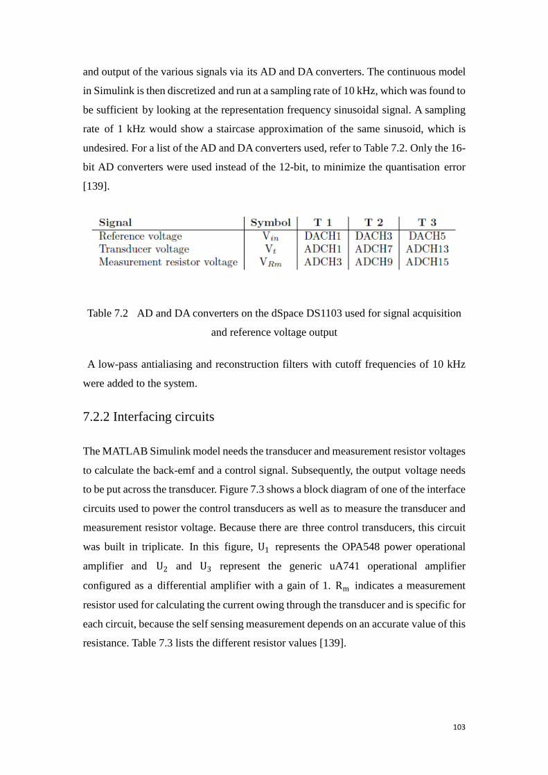
103
and output of the various signals via its AD and DA converters. The continuous model
in Simulink is then discretized and run at a sampling rate of 10 kHz, which was found to
be sufficient by looking at the representation frequency sinusoidal signal. A sampling
rate of 1 kHz would show a staircase approximation of the same sinusoid, which is
undesired. For a list of the AD and DA converters used, refer to Table 7.2. Only the 16-
bit AD converters were used instead of the 12-bit, to minimize the quantisation error
[139].
Table 7.2 AD and DA converters on the dSpace DS1103 used for signal acquisition
and reference voltage output
A low-pass antialiasing and reconstruction filters with cutoff frequencies of 10 kHz
were added to the system.
7.2.2 Interfacing circuits
The MATLAB Simulink model needs the transducer and measurement resistor voltages
to calculate the back-emf and a control signal. Subsequently, the output voltage needs
to be put across the transducer. Figure 7.3 shows a block diagram of one of the interface
circuits used to power the control transducers as well as to measure the transducer and
measurement resistor voltage. Because there are three control transducers, this circuit
was built in triplicate. In this figure, U1 represents the OPA548 power operational
amplifier and U2 and U3 represent the generic uA741 operational amplifier
configured as a differential amplifier with a gain of 1. Rm indicates a measurement
resistor used for calculating the current owing through the transducer and is specific for
each circuit, because the self sensing measurement depends on an accurate value of this
resistance. Table 7.3 lists the different resistor values [139].
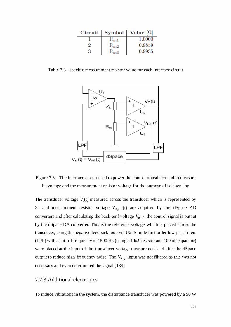
104
Table 7.3 specific measurement resistor value for each interface circuit
Figure 7.3 The interface circuit used to power the control transducer and to measure
its voltage and the measurement resistor voltage for the purpose of self sensing
The transducer voltage Vt(t) measured across the transducer which is represented by
ZL and measurement resistor voltage VRm (t) are acquired by the dSpace AD
converters and after calculating the back-emf voltage Vemf , the control signal is output
by the dSpace DA converter. This is the reference voltage which is placed across the
transducer, using the negative feedback loop via U2. Simple first order low-pass filters
(LPF) with a cut-off frequency of 1500 Hz (using a 1 kΩ resistor and 100 nF capacitor)
were placed at the input of the transducer voltage measurement and after the dSpace
output to reduce high frequency noise. The VRm input was not filtered as this was not
necessary and even deteriorated the signal [139].
7.2.3 Additional electronics
To induce vibrations in the system, the disturbance transducer was powered by a 50 W

105
Jaycar amplifier kit. A sinusoid signal was used as input signal, which frequency was
chosen from 20 to 50 Hz.
7.3 Multi-mode SISO PPF Controller Experiment
Implemented Result
Three SISO PPF controller are used to control the first four vibration modes of
simulation plate structure model. Firstly, Three SISO PPF controller are formed in
MATLAB Simulink. Secondly, sinusoid signals which contain resonant frequencies of
first four modes of simulation plate structure model are applied to the shaker one by
one. Thirdly, Open-loop dynamics which is between shaker to plate without controller
is compared to closed-loop dynamics which is between shaker to plate with controller.
Time domain cases are designed to test the ability of three SISO PPF controller to
attenuate multi-mode vibration when the controller centre frequencies match the
resonant frequencies of the plate. The following is the multi-mode three SISO
vibration control experiment results for every mode at each transducer.
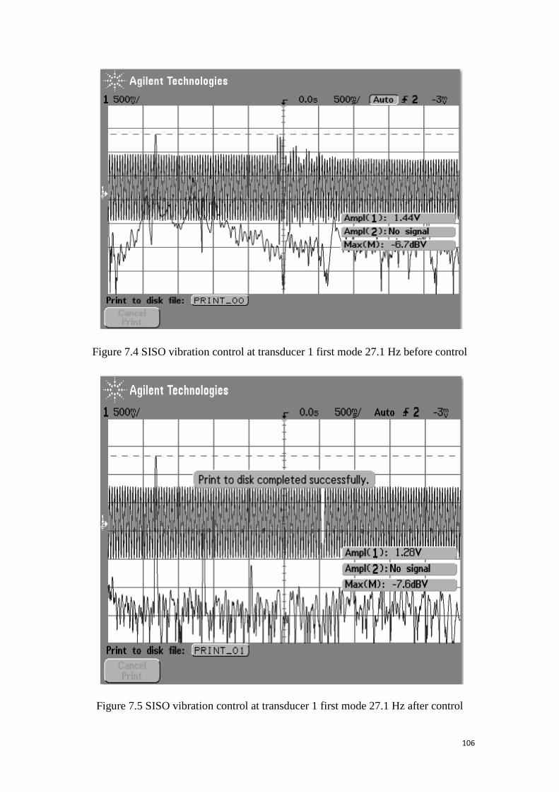
106
Figure 7.4 SISO vibration control at transducer 1 first mode 27.1 Hz before control
Figure 7.5 SISO vibration control at transducer 1 first mode 27.1 Hz after control

107
Figure 7.6 SISO vibration control at transducer 1 second mode 34.4 Hz before control
Figure 7.7 SISO vibration control at transducer 1 second mode 34.4 Hz after control

108
Figure 7.8 SISO vibration control at transducer 1 third mode 40.5 Hz before control
Figure 7.9 SISO vibration control at transducer 1 third mode 40.5 Hz SISO after
control

109
Figure 7.10 SISO vibration control at transducer 1 forth mode 49.2 Hz before control
Figure 7.11 SISO vibration control at transducer 1 forth mode 49.2 Hz after control

110
Figure 7.12 SISO vibration control at transducer 2 first mode 27.1Hz before control
Figure 7.13 SISO vibration control at transducer 2 first mode 27.1Hz SISO after
control

111
Figure 7.14 SISO vibration control at transducer 2 second mode 34.4 Hz before
control
Figure 7.15 SISO vibration control at transducer 2 second mode 34.4 Hz after control

112
Figure 7.16 SISO vibration control at transducer 2 third mode 40.5 Hz before control
Figure 7.17 SISO vibration control at transducer 2 third mode 40.5 Hz after control
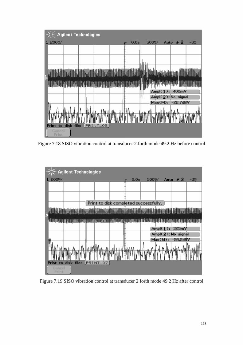
113
Figure 7.18 SISO vibration control at transducer 2 forth mode 49.2 Hz before control
Figure 7.19 SISO vibration control at transducer 2 forth mode 49.2 Hz after control
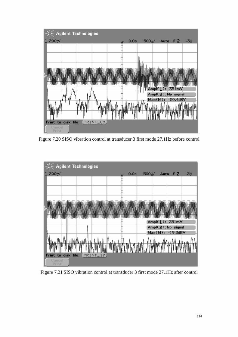
114
Figure 7.20 SISO vibration control at transducer 3 first mode 27.1Hz before control
Figure 7.21 SISO vibration control at transducer 3 first mode 27.1Hz after control
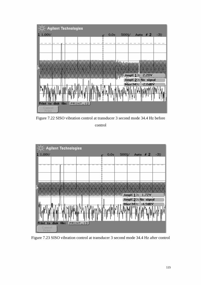
115
Figure 7.22 SISO vibration control at transducer 3 second mode 34.4 Hz before
control
Figure 7.23 SISO vibration control at transducer 3 second mode 34.4 Hz after control

116
Figure 7.24 SISO vibration control at transducer 3 third mode 40.5 Hz before control
Figure 7.25 SISO vibration control at transducer 3 third mode 40.5 Hz after control
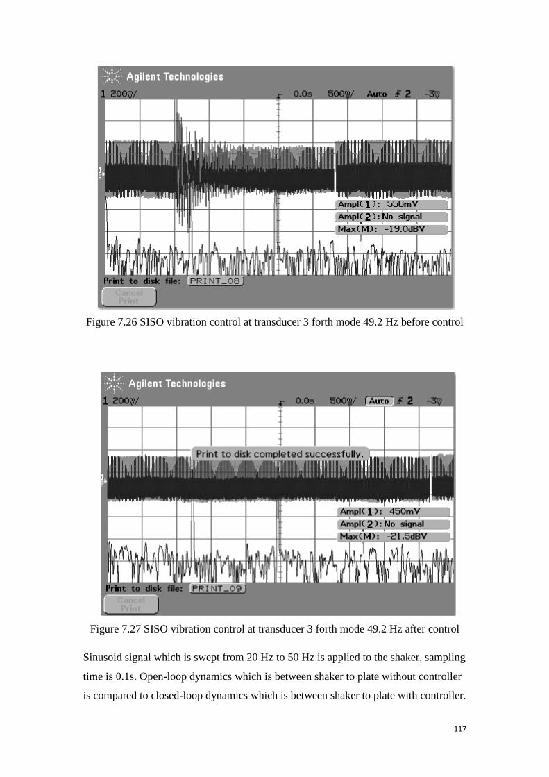
117
Figure 7.26 SISO vibration control at transducer 3 forth mode 49.2 Hz before control
Figure 7.27 SISO vibration control at transducer 3 forth mode 49.2 Hz after control
Sinusoid signal which is swept from 20 Hz to 50 Hz is applied to the shaker, sampling
time is 0.1s. Open-loop dynamics which is between shaker to plate without controller
is compared to closed-loop dynamics which is between shaker to plate with controller.
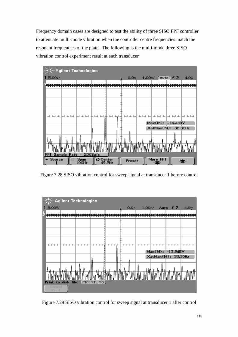
118
Frequency domain cases are designed to test the ability of three SISO PPF controller
to attenuate multi-mode vibration when the controller centre frequencies match the
resonant frequencies of the plate . The following is the multi-mode three SISO
vibration control experiment result at each transducer.
Figure 7.28 SISO vibration control for sweep signal at transducer 1 before control
Figure 7.29 SISO vibration control for sweep signal at transducer 1 after control

119
Figure 7.30 SISO vibration control for sweep signal at transducer 2 before control
Figure 7.31 SISO vibration control for sweep signal at transducer 2 after control
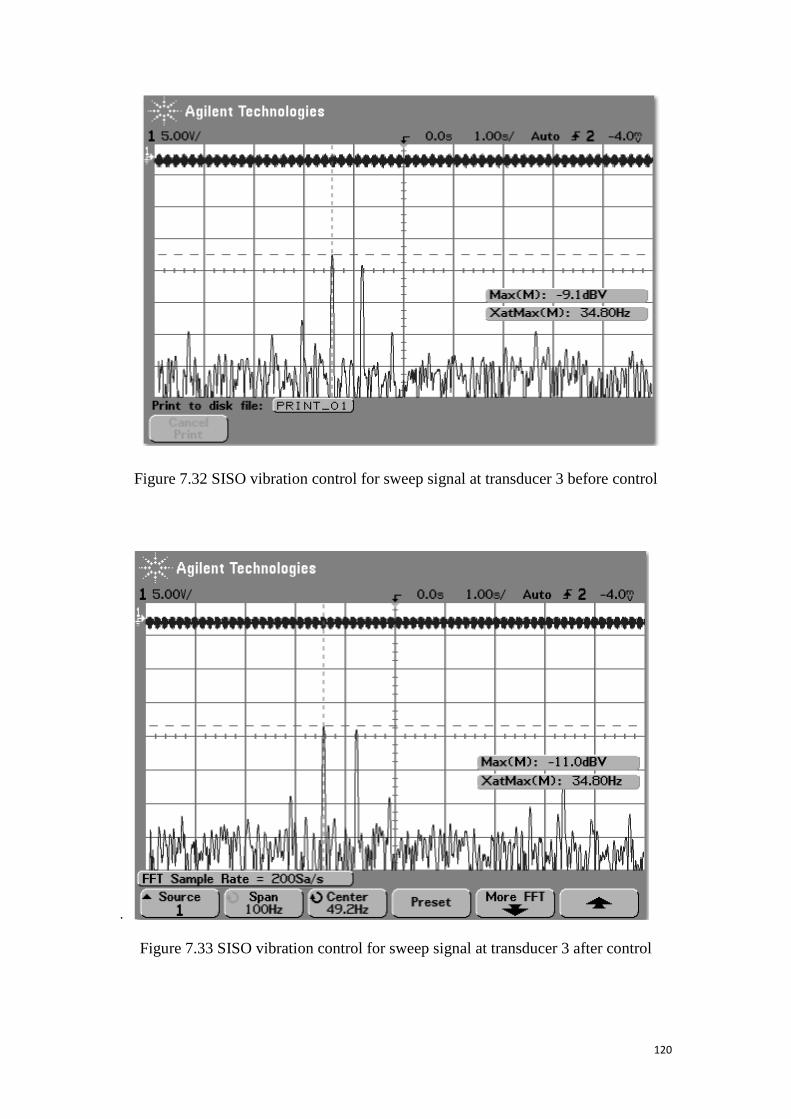
120
Figure 7.32 SISO vibration control for sweep signal at transducer 3 before control
.
Figure 7.33 SISO vibration control for sweep signal at transducer 3 after control

121
The final experimental results for three SISO PPF controller are given in the Table
7.4.
frequency (Hz)
27.1 34.4 40.5 49.2
transduer 1
Acceleration (g) before 1.44 1.53 0.77 5.06
after 1.28 1.2 0.75 4.44
reduce rate (%) 11.11% 21.569% 2.5974% 12.253%
Max Peak (dB) before -6.7 -6.0 -13.7 4.8
after -7.6 -8.2 -13.7 3.4
reduce(dB) 0.9 2.2 0 1.4
transduer 2
Acceleration (g) before 0.388 2.75 2.47 0.4
after 0.25 2.16 2.09 0.325
reduce rate(%) 35.57% 21.45% 15.38% 18.75%
Max Peak (dB) before -20.3 -0.8 -1.7 -22.7
after -26.1 -2.9 -3.1 -26.5
Reduce (dB) 5.8 2.1 1.4 3.8
transduer 3
Acceleration (g) before 0.381 2.28 2.28 0.556
after 0.381 1.72 1.91 0.45
reduce rate(%) 0 24.561% 16.228% 19.065%
Max Peak (dB) before -20.4 -2.6 -2.5 -19
after -19.3 -4.9 -4.2 -21.5
Reduce (dB) -1.1 2.3 1.7 2.5
Table 7.4 SISO vibration control experimental results
The parameters of the three SISO PPF controller are given in Table 7.5.
Mode 1 Mode 2 Mode 3 Mode 4
Controller control g1=6.9 g2=2.19E-02 g3=1.54E-03 g4=1.05E-03

122
K11 gain
damping zc1=5.87E-02 zc2=0.351 zc3=0.295 zc4=0.243
Controller
K22
control
gain g5=0.345 g6=6.58E-02 g7=1.54E-03 g8=1.05E-03
damping zc5=5.87E-02 zc6=3.51E-01 zc7=2.95E-01 zc8=2.43E-01
Controller
K33
control
gain g9=3.45E-01 g10=2.19E-01 g11=1.54E-03 g12=1.05E-03
damping zc9=5.87E-02 zc10=3.51E-01 zc11=2.95E-01 zc12=2.43E-01
Table 7.5 multi-mode SISO PPF controller experimental parameter result
7.4 Multi-mode MIMO PPF Controller Experimental
Implemented Result
MIMO PPF controller are used to control the first four vibration modes of simulation
plate structure model. Firstly, MIMO PPF controller are formed in MATLAB
Simulink. Secondly, sinusoid signals which contain resonant frequencies of first four
modes of simulation plate structure model are applied to the shaker one by one.
Thirdly, Open-loop dynamics which is between shaker to plate without controller is
compared to closed-loop dynamics which is between shaker to plate with controller.
Time domain cases are designed to test the ability of MIMO PPF controller to
attenuate multi-mode vibration when the controller centre frequencies match the
resonant frequencies of the plate. The following is the multi-mode MIMO PPF
vibration control experiment results.

123
Mode 1 Mode 2 Mode 3 Mode 4
Controller 1
control
gain g1=0.103E g2=6.58 g3=1.54E-03 g4=1.06
damping zc1=0.006 zc2=0.818 zc3=0.987 zc4=0.013
Controller 2
control
gain g5=2.94E-04 g6=2.34E-02 g7=1.96E-02 g8=1.62E-02
damping zc5=0.001 zc6=0.668 zc7=0.029 zc8=0.086
Controller 3
control
gain g9=1.47E-02 g10=2.34E-02 g11=3.93E-02 g12=1.62E-02
damping zc9=2.94E-02 zc10=4.68E-02 zc11=1.96E-0 zc12=1.62E-02
Table 7.6 multi-mode MIMO PPF controller parameter result
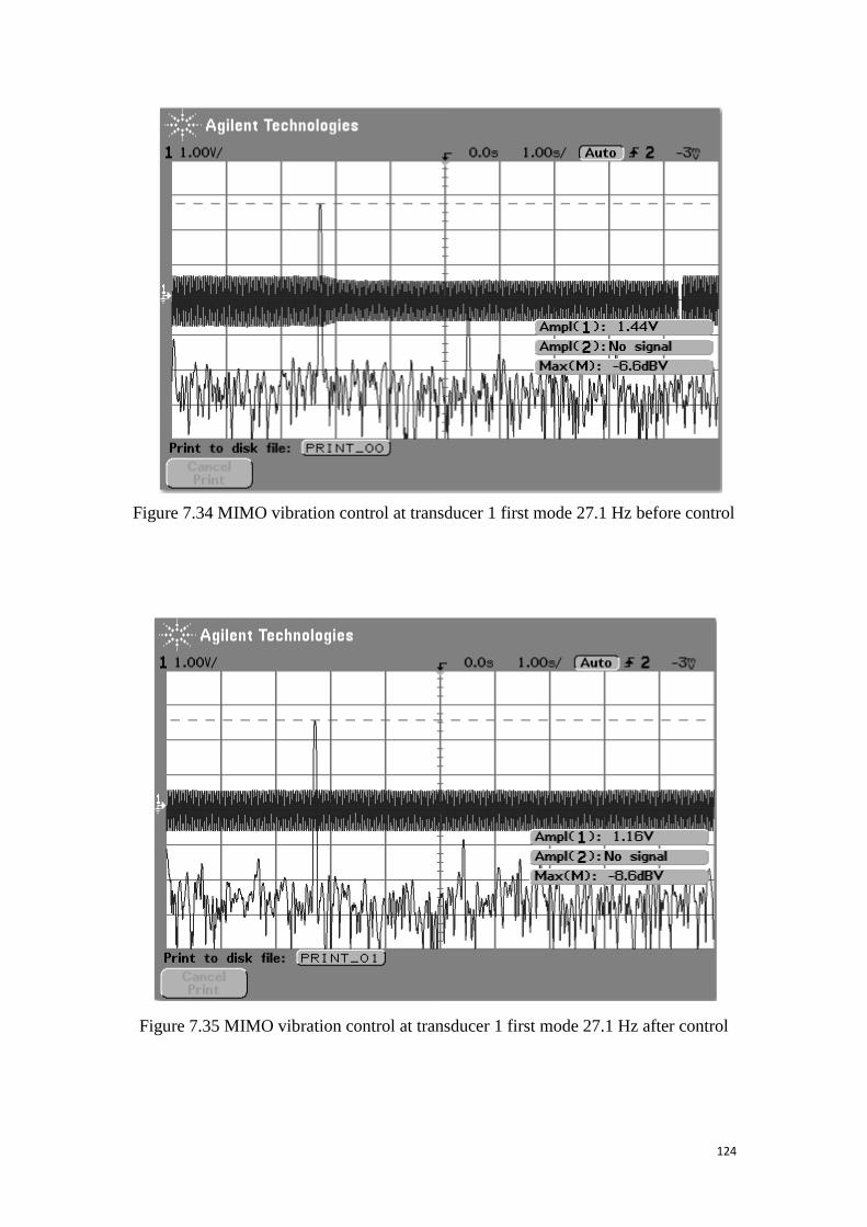
124
Figure 7.34 MIMO vibration control at transducer 1 first mode 27.1 Hz before control
Figure 7.35 MIMO vibration control at transducer 1 first mode 27.1 Hz after control

125
Figure 7.36 MIMO vibration control at transducer 1 second mode 34.4 Hz before
control
Figure 7.37 MIMO vibration control at transducer 1 second mode 34.4 Hz after
control
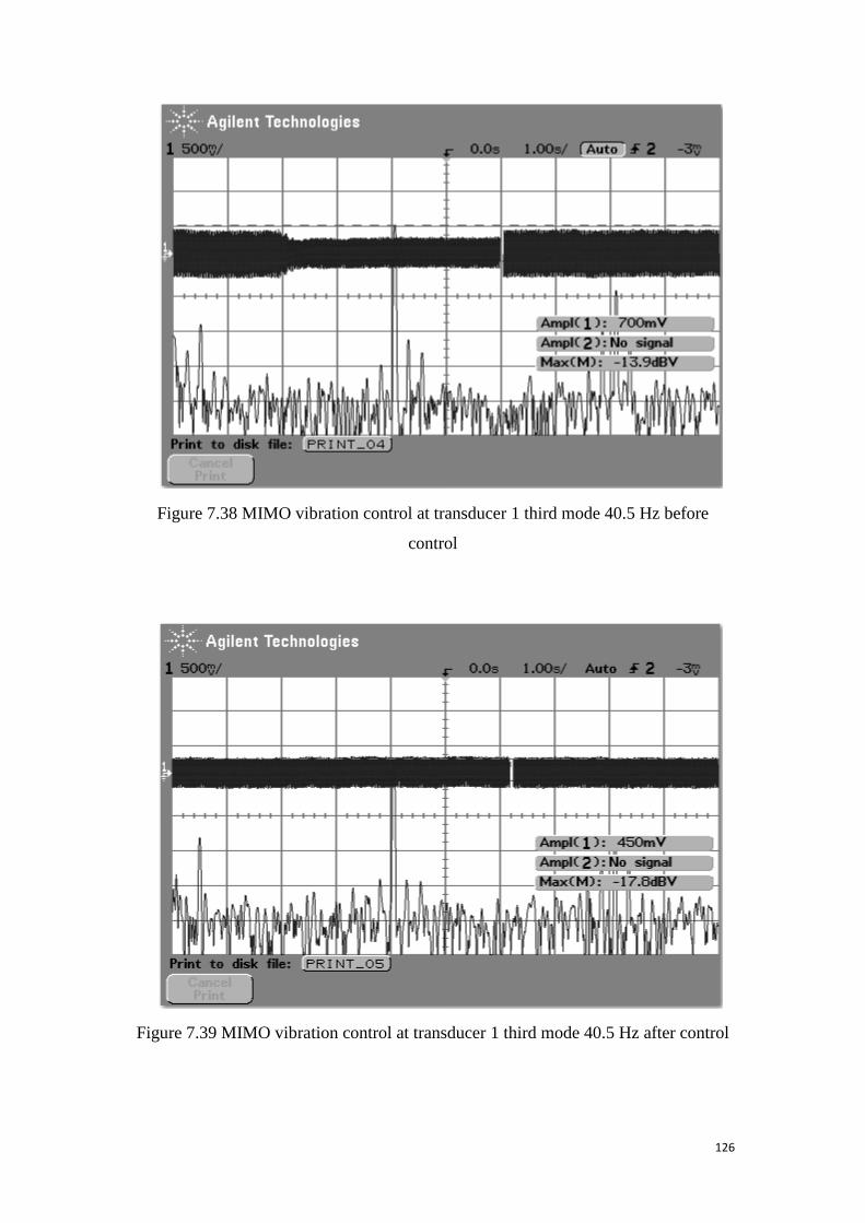
126
Figure 7.38 MIMO vibration control at transducer 1 third mode 40.5 Hz before
control
Figure 7.39 MIMO vibration control at transducer 1 third mode 40.5 Hz after control

127
Figure 7.40 MIMO vibration control at transducer 1 forth mode 49.2 Hz before
control
Figure 7.41 MIMO vibration control at transducer 1 forth mode 49.2 Hz after control

128
Figure 7.42 MIMO vibration control at transducer 2 first mode 27.1Hz before control
Figure 7.43 MIMO vibration control at transducer 2 first mode 27.1Hz after control

129
Figure 7.44 MIMO vibration control at transducer 2 second mode 34.4 Hz before
control
Figure 7.45 MIMO vibration control at transducer 2 second mode 34.4 Hz after
control

130
Figure 7.46 MIMO vibration control at transducer 2 third mode 40.5 Hz before
control
Figure 7.47 MIMO vibration control at transducer 2 third mode 40.5 Hz after control

131
Figure 7.48 MIMO vibration control at transducer 2 forth mode 49.2 Hz before
control
Figure 7.49 MIMO vibration control at transducer 2 forth mode 49.2 Hz after control
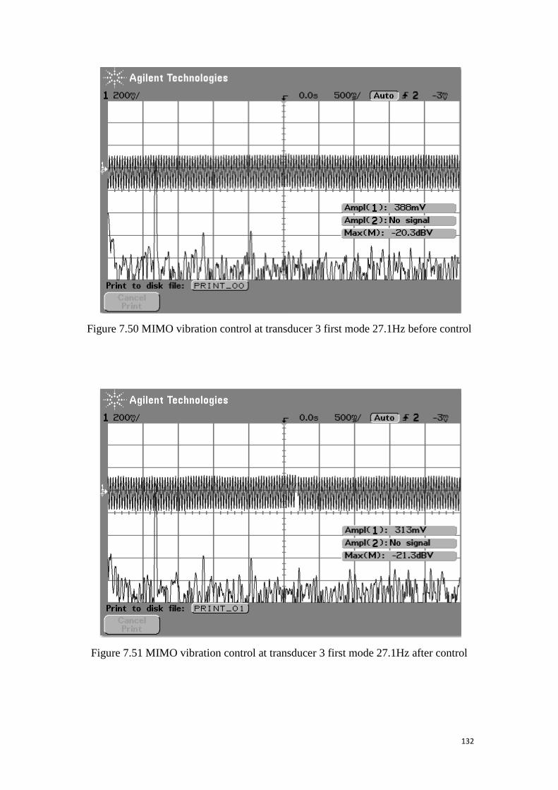
132
Figure 7.50 MIMO vibration control at transducer 3 first mode 27.1Hz before control
Figure 7.51 MIMO vibration control at transducer 3 first mode 27.1Hz after control

133
Figure 7.52 MIMO vibration control at transducer 3 second mode 34.4 Hz before
control
Figure 7.53 MIMO vibration control at transducer 3 second mode 34.4 Hz after
control

134
Figure 7.54 MIMO vibration control at transducer 3 third mode 40.5 Hz before
control
Figure 7.55 MIMO vibration control at transducer 3 third mode 40.5 Hz after control

135
Figure 7.56 MIMO vibration control at transducer 3 forth mode 49.2 Hz before
control
Figure 7.57 MIMO vibration control at transducer 3 forth mode 49.2 Hz after control
Sinusoid signal which is swept from 20 Hz to 50 Hz is applied to the shaker, sampling
time is 0.1s. Open-loop dynamics which is between shaker to plate without controller
is compared to closed-loop dynamics which is between shaker to plate with controller.
Frequency domain cases are designed to test the ability of MIMO controller to
attenuate multi-mode vibration when the controller centre frequencies match the

136
resonant frequencies of the plate . The following is the multi-mode MIMO vibration
control experiment result at each transducer.
Figure 7.58 MIMO vibration control for sweep signal at transducer 1 before control
Figure 7.59 MIMO vibration control for sweep signal at transducer 1 after control

137
Figure 7.60 MIMO vibration control for sweep signal at transducer 2 before control
Figure 7.61 MIMO vibration control for sweep signal at transducer 2 after control

138
Figure 7.63 MIMO vibration control for sweep signal at transducer 3 before control
Figure 7.63 MIMO vibration control for sweep signal at transducer 3 after control

139
The parameters of the MIMO PPF controller are given in Table 7.7.
frequency (Hz)
27.1 34.4 40.5 49.2
transduer 1
Acceleration (g) before 1.44 1.56 0.7 4.81
after 1.16 1.13 0.45 4.13
reduce rate (%) 19.444% 27.64% 35.714% 14.137%
Max Peak (dB) before -6.6 -6.2 -13.9 4.2
after -8.6 -8.9 -17.8 2.7
reduce(dB) 2 2.7 3.9 1.5
transduer 2
Acceleration (g) before 0.294 2.75 2.16 0.35
after 0.194 2.22 0.88 0.287
reduce rate(%) 34.01% 19.27% 59.26% 18%
Max Peak (dB) before -22.6 -0.8 -3.1 -22.5
after -27.6 -2.8 -11.5 -23.5
Reduce (dB) 5 2 7.6 1
transduer 3
Acceleration (g) before 0.388 2.34 1.84 0.55
after 0.313 1.56 0.91 0.39
reduce rate(%) 19.33% 33.333% 50.543% 29.091%
Max Peak (dB) before -20.3 -2.3 -4.3 -20.4
after -21.3 -5.7 -11.2 -22.4
Reduce (dB) 1 3.4 6.9 2
Table 7.7 multi-mode MIMO vibration control experimental results
7.5 Summary
Although we try to derive the mathematical model which has the same dynamics
response as the experimental plant, the parameters of the multi-mode SISO and
MIMO PPF controllers in the experimental study are still different from the ones in
simulation study because during modelling, we simplified the structure of transducer
which is more complicated with electromagnetic and nonlinear characters in the fact.

140
For multi-mode three SISO PPF controller, the open-loop and closed-loop time
domain and frequency domain results can be seen through Figure 7.4-7.33 and Table
7.4, 7.5.
It can be seen in the figure that at the beginning of turning on controller, there was a
noise happened.
From a mathematical point of view, when the control is off, the transfer function is
simply that of a monic vibrating system subjected to an arbitrary impulse. When the
control comes on, the transfer function that describes the input-output relationship
between the sensor and actuator takes over, however, its denominator remains the
same, while its numerator will be altered [64].
Physically, this is due to the fact that for the collocated sensor/actuator pair (in the
experiment, sensor and actuator is the same one) there will be some direct energy
transmission from the actuator to the sensor. Thus the sensor voltage is made up of
two components, some of the response due to the actuator, and some direct
transmission of the force due to the collocation of the actuator [64].
However, this is not a problem for the PPF control law, as it was proven to be stable
even in the presence control law of feed through in Chapter 5.3.
For sweep signal multi-mode three SISO vibration control result, it did not show the
attenuation at each mode as in simulation.
For multi-mode MIMO PPF controller, the open-loop and closed-loop results can be
seen through Figure 7.34-7.63 and Table 7.5, 7.6. It is shown a better result
comparing with multi-mode three SISO PPF controller and there is no noise happened
at the beginning of turning on controller.
For the first mode, the performance of multi-mode MIMO PPF controller is not good,
because there is only one transducer (transducer 1) at that side, but there are two
degrees of freedom at the corners (bending and torsion which could be seen in the
ANSYS result Fig 2.13), one transducer is not enough to control two degrees of
freedom vibration at the same time.

141
Same with mode 3 and mode 4, the performance of multi-mode MIMO controllers
was decreased because only one transducer is not enough to control two degrees of
freedom vibration at the same time.
For sweep signal multi-mode MIMO vibration control result, due to the limitation of
oscilloscope which can only read the max(M) result, it could get the exactly
attenuation result at each mode, but the attenuation at each mode still can be seen
from the figure.

142
Chapter 8
Conclusion and Future Work
8.1 Outcomes of the Research
Because the increasing demand for improving dynamic performance, the operating
efficiency, and the amount of material which is used in mechanical structures, many
designers employ lightweight materials to reduce the cross sectional dimensions of
those structures.
Due to the side-effect of employing lightweight materials and reducing the cross
sectional dimensions, the structures become more flexible and more susceptible to the
detrimental effects of unwanted vibration, particularly when they operate at or near
their natural frequencies or when they are excited by disturbances that coincide with
their natural frequencies.
The design and implementation of a high performance vibration controller for a flexible
structure can be a so important task. In order to complete the task and achieve better
performance, in this thesis, the author did the following things:
Firstly, based on experimental, analytical and numerical three kinds of analysis
methods, an infinite-dimensional and a very high-order mathematical transfer
function model for distributed parameter plate structure is derived, using modal
analysis and numerical analysis results. A 47 modes plate model was given as the
simulation model.
Secondly, traditional balanced model reduction method is used to decrease the
dimensions and orders of the plate simulation model.
Thirdly, a four modes feed-through truncated plate model which minimizing the
effect of other truncated modes on spatial low-frequency dynamics of the system
by adding a spatial zero frequency term to the truncated model is provided.

143
Numerical software MATLAB is used to compare the feed-through truncated
plate model with balanced reduction plate model.
Fourthly, both multi-mode SISO and MIMO PPF active control laws based upon
positive position feedback is proposed, developed and studied for the flexible
plate structure with bonded three self-sensing magnetic transducers which
guarantee unconditional stability of the closed-loop system similar as collocated
control system. The proposed multi-mode SISO and MIMO PPF controllers can
be tuned to the chosen first four modes of the plate structure and increased the
damping of the plate so as to minimize the chosen resonant responses. Stability
conditions for scalar and multivariable case of PPF controllers are derived,
multivariable case which allow for a feed-through term in the model is also
derived, which is needed to ensure little perturbation in the in-bandwidth zeros of
the model. In order to derive optimal controller parameters, a minimization
criterion based on the H∞ norm of the closed-loop system is solved by a genetic
algorithm.
Fifthly, the proposed multi-mode MIMO PPF controller, compared with
multi-mode SISO PPF controller, which is validated in both simulations and
experimental implementation, is an effective solution to suppress the vibration of
distributed parameter plate structure.
According to literature review, the proposed multi-mode active vibration control
methodology for plate structure using H∞ optimization MIMO positive position
feedback based genetic algorithm is the first time, similar method only can be found
such as SISO PPF using H∞ optimization based on genetic algorithm applied on
beam structure[65], MIMO PPF using H∞ optimization and pole optimization
applied on beam structure[1, 3] .
8.2 Future Work
Within the scope of the research project documented herein, the development and
implementation of multi-mode active vibration control methodology for plate
structure using H∞ optimization positive position feedback based genetic algorithm
is focused on an MIMO basis. Due to the limited time and other restrained conditions,
some parts of the experimental study may need to improve in the future.
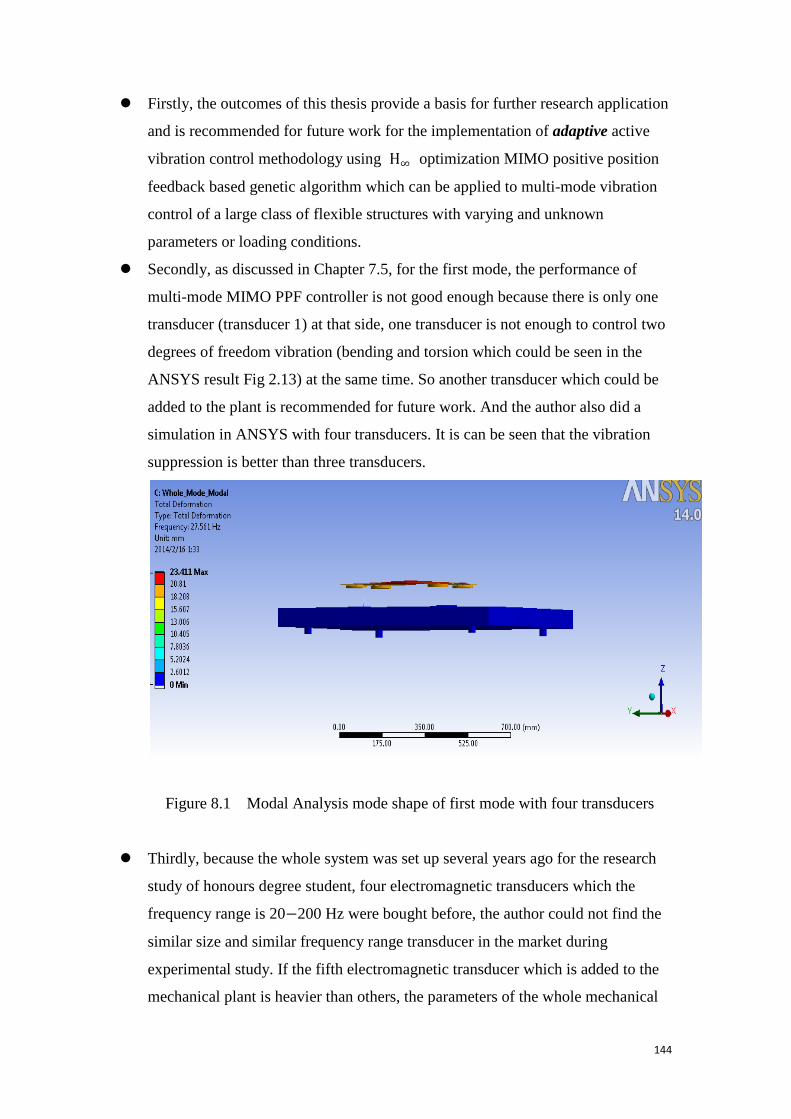
144
Firstly, the outcomes of this thesis provide a basis for further research application
and is recommended for future work for the implementation of adaptive active
vibration control methodology using H∞ optimization MIMO positive position
feedback based genetic algorithm which can be applied to multi-mode vibration
control of a large class of flexible structures with varying and unknown
parameters or loading conditions.
Secondly, as discussed in Chapter 7.5, for the first mode, the performance of
multi-mode MIMO PPF controller is not good enough because there is only one
transducer (transducer 1) at that side, one transducer is not enough to control two
degrees of freedom vibration (bending and torsion which could be seen in the
ANSYS result Fig 2.13) at the same time. So another transducer which could be
added to the plant is recommended for future work. And the author also did a
simulation in ANSYS with four transducers. It is can be seen that the vibration
suppression is better than three transducers.
Figure 8.1 Modal Analysis mode shape of first mode with four transducers
Thirdly, because the whole system was set up several years ago for the research
study of honours degree student, four electromagnetic transducers which the
frequency range is 20−200 Hz were bought before, the author could not find the
similar size and similar frequency range transducer in the market during
experimental study. If the fifth electromagnetic transducer which is added to the
mechanical plant is heavier than others, the parameters of the whole mechanical

145
plant may change hugely, for example, the frequency of the first mode may drop
down and below 20 Hz, which is beyond the frequency range of the transducer, or
just a little bit over 20Hz, which is in the strongly nonlinear output area of the
electromagnetic transducer and very hard to control the vibration of plate . So it is
recommended for future that make a same size and same frequency range
transducer by hand if could not find in the market, either.
Fourthly, because the limitation of electromagnetic transducer, such as the
frequency range only between 20−200 Hz, the limitation of the oscilloscope
which can only read the max(M) result, piezoelectric sensor and actuator, signal
analyzer are recommended for future experimental study to instead of the old
equipments.
Fifthly, as stated in 1.5.3 of Chapter 1, PPF combine with Genetic Algorithms
(GA), the optimal control position of the three control transducers is also
recommended for future work, which could be derived through GA calculation.
Sixthly, although the author try to derive the mathematical model which has the
same dynamic response as the experimental plant, the parameters of the
multi-mode SISO and MIMO PPF controllers in the experimental study are still
different from the ones in the simulation study because during modelling, the
author simplified the structure of the transducer which is more complicated with
electromagnetic and nonlinear characters in the fact. So it is recommended to
remodel the transducer and minimize the effect to the whole system for future
work.

146
Bibliography [1] Moheimani, S. O. R., Vautier, B. J. G., & Bhilkkaji, B. (2005, December).
Multivariable PPF control of an active structure. In Decision and Control, 2005
and 2005 European Control Conference. CDC-ECC'05. 44th IEEE Conference on
(pp. 6824-6829). IEEE
[2] Halim, D., & Moheimani, S. O. (2004). Reducing the effect of truncation error in
spatial and pointwise models of resonant systems with damping. Mechanical
systems and signal processing, 18(2), 291-315
[3] Moheimani, S. R., Vautier, B. J., & Bhikkaji, B. (2006). Experimental
implementation of extended multivariable PPF control on an active structure.
Control Systems Technology, IEEE Transactions on, 14(3), 443-455
[4] Tjahyadi, H. (2007). Adaptive multi mode vibration control of dynamically
loaded flexible structures (Doctoral dissertation, Flinders University)
[5] P Micheau and P. Coirault. Adaptive controller using filter banks to reject
multi-sinusoidal disturbance. Automatica, 36:1659–1664, 2000.
[6] D.J. Inman. Engineering Vibration. Prentice Hall, USA, 1996.
[7] Andre Preumont, Kazuto Seto. Active control of structures, UK, 2008
[8] Dorf, R. C. (1991). Modern control systems. Addison-Wesley Longman
Publishing Co., Inc..
[9] Genta, G. (2009). Vibration dynamics and control. Springer.
[10] Haugen, F. (2010). Basic Dynamics and Control. Porsgrunn: TeachTech.
[11] Belgacem, W., Berry, A., & Masson, P. (2012). Active vibration control on a
quarter-car for cancellation of road noise disturbance. Journal of Sound and
Vibration, 331(14), 3240-3254
[12] Yong, S., Zhiyuan, G., Shouwe, G., Jincong, Y., & Xiaojin, Z. (2010, July).
FXLMS algorithm based multi channel active vibration control of piezoelectric
flexible beam. In Intelligent Control and Automation (WCICA), 2010 8th World
Congress on (pp. 4845-4850). IEEE.

147
[13] Li, D. S., & Cheng, L. (2010). The design of synthesized structural acoustic
sensors for active control of interior noise with experimental validation. Journal
of Sound and Vibration, 329(2), 123-139
[14] Preumont, A. (1999). Vibration control of active structures: an introduction.
Meccanica, 34(2), 139-139.
[15] C.R. Fuller, S.J. Elliott, and P.A. Nelson. Active Control of Vibration.
Academic Press, London, 1996.
[16] Iwamoto, H., Tanaka, N., & Hill, S. G. (2012). Feedback control of wave
propagation in a rectangular panel, part 2: Experimental realization using
clustered velocity and displacement feedback. Mechanical Systems and Signal
Processing.
[17] Li, S. (2011). Active modal control simulation of vibro-acoustic response of a
fluid-loaded plate. Journal of Sound and Vibration, 330(23), 5545-5557
[18] Kim, S. M., & Oh, J. E. (2013). A modal filter approach to non-collocated
vibration control of structures. Journal of Sound and Vibration
[19] Meirovitch, L., Van Landingham, H. F., & Öz, H. (1977). Control of spinning
flexible spacecraft by modal synthesis. Acta Astronautica, 4(9), 985-1010
[20] Meirovitch, L., Baruh, H., & OZ, H. (1983). A comparison of control techniques
for large flexible systems. Journal of Guidance, Control, and Dynamics, 6(4),
302-310
[21] Moheimani, S. O. R., Fleming, A. J., & Behrens, S. (2001). Highly resonant
controller for multimode piezoelectric shunt damping. Electronics Letters, 37(25),
1505-1506
[22] Pota, H. R., Moheimani, S. R., & Smith, M. (2002). Resonant controllers for
smart structures. Smart Materials and Structures, 11(1), 1
[23] Aphale, S. S., Fleming, A. J., & Moheimani, S. R. (2007). Integral resonant
control of collocated smart structures. Smart Materials and Structures, 16(2), 439.
[24] Pereira, E., Moheimani, S. O. R., & Aphale, S. S. (2008). Analog implementation
of an integral resonant control scheme. Smart Materials and Structures, 17(6),
067001.
[25] Mahmood, I. A., Moheimani, S. R., & Bhikkaji, B. (2008). Precise tip positioning
of a flexible manipulator using resonant control. Mechatronics, IEEE/ASME
Transactions on, 13(2), 180-186.
148
[26] Pereira, E., Aphale, S. S., Feliu, V., & Moheimani, S. R. (2011). Integral resonant
control for vibration damping and precise tip-positioning of a single-link flexible
manipulator. Mechatronics, IEEE/ASME Transactions on, 16(2), 232-240
[27] Halim, D., & Moheimani, S. R. (2001). Spatial resonant control of flexible
structures-application to a piezoelectric laminate beam. Control Systems
Technology, IEEE Transactions on, 9(1), 37-53
[28] Goh, C. J. (1983). Analysis and control of quasi distributed parameter systems
(Doctoral dissertation, California Institute of Technology).
[29] Goh, C. J., & Caughey, T. K. (1985). On the stability problem caused by finite
actuator dynamics in the collocated control of large space structures. International
Journal of Control, 41(3), 787-802
[30] Fanson J L, An experimental investigation of vibration suppression in large space
structures using positive position feedback, PhD Thesis California Institute of
Technology,November,1986
[31] J. L. Fanson, and T. K. Caughey, "Positive Position Feedback Control for Large
Space Structures," AIAA Journal, vol. 28, no. 4, pp.717-724, 1990
[32] Song G, Schmidt S P and Agrawal B N, Experimental robustness study of
positive position feedback control for active vibration suppression, J. Guidance,
VOL. 25, NO. 1: ENGINEERING NOTES, 2001
[33] Baz, A., Poh, S., & Fedor, J. (1989). Independent modal space control with
positive position feedback. Dynamics and control of large structures, 553-567
[34] Poh, S., & Baz, A. (1990). Active control of a flexible structure using a modal
positive position feedback controller. Journal of Intelligent Material Systems and
Structures, 1(3), 273-288.
[35] Goh, C. J., & Lee, T. H. (1991). Adaptive modal parameters identification for
collocated position feedback vibration control. International Journal of Control,
53(3), 597-617.
[36] Caughey, T. K. (1995). Dynamic response of structures constructed from smart
materials. Smart Materials and Structures, 4(1A), A101
[37] Baz, A., & Poh, S. (1996). Optimal vibration control with modal positive position
feedback. Optimal control applications and methods, 17(2), 141-149

149
[38] Baz, A., & HONG, J. T. (1997). Adaptive control of flexible structures using
modal positive position feedback. International journal of adaptive control and
signal processing, 11(3), 231-253
[39] Wang, L. (2003, October). Positive position feedback based vibration attenuation
for a flexible aerospace structure using multiple piezoelectric actuators. In Digital
Avionics Systems Conference, 2003. DASC'03. The 22nd (Vol. 2, pp. 7-C).
IEEE.
[40] Shan, J., Liu, H. T., & Sun, D. (2005). Slewing and vibration control of a
single-link flexible manipulator by positive position feedback (PPF).
Mechatronics, 15(4), 487-503.
[41] Hong, C., Shin, C., & Jeong, W. (2010). Active vibration control of clamped
beams using PPF controllers with piezoceramic actuators. Proc. 20th Int. Congr.
on Acoustics (Sydney, Australia, ICA 2010 23–27 August 2010).
[42] Ahmed, B., & Pota, H. R. (2011). Dynamic compensation for control of a rotary
wing UAV using positive position feedback. Journal of Intelligent & Robotic
Systems, 61(1-4), 43-56.
[43] Chuang, K. C., Ma, C. C., & Wu, R. H. (2012). Active suppression of a beam
under a moving mass using a pointwise fiber bragg grating displacement sensing
system. Ultrasonics, Ferroelectrics and Frequency Control, IEEE Transactions on,
59(10), 2137-2148.
[44] Shin, C., Hong, C., & Jeong, W. B. (2012). Active vibration control of clamped
beams using positive position feedback controllers with moment pair. Journal of
mechanical science and technology, 26(3), 731-740.
[45] Bang, H., & Agrawal, B. N. (1994). A generalized second order compensator
design for vibration control of flexible structures. In
AIAA/ASME/ASCE/AHS/ASC Structures, Structural Dynamics, and Materials
Conference, 35th, Hilton Head, SC (pp. 2438-2448).
[46] Mahmoodi, S. N., Aagaah, M. R., & Ahmadian, M. (2009, June). Active vibration
control of aerospace structures using a modified positive position feedback
method. In American Control Conference, 2009. ACC'09. (pp. 4115-4120). IEEE
[47] Hu, Q., Xie, L., & Gao, H. (2006, December). A combined positive position
feedback and variable structure approach for flexible spacecraft under input

150
nonlinearity. In Control, Automation, Robotics and Vision, 2006. ICARCV'06.
9th International Conference on (pp. 1-6). IEEE.
[48] Hu, Q., Xie, L., & Gao, H. (2007). Adaptive variable structure and active
vibration reduction for flexible spacecraft under input nonlinearity. Journal of
Vibration and Control, 13(11), 1573-1602. [49] Kim, S. M., Wang, S., & Brennan, M. J. (2011). Comparison of negative and
positive position feedback control of a flexible structure. Smart Materials and
Structures, 20(1), 015011.
[50] Bhikkaji, B., Ratnam, M., Fleming, A. J., & Moheimani, S. R. (2007).
High-performance control of piezoelectric tube scanners. Control Systems
Technology, IEEE Transactions on, 15(5), 853-866.
[51] Chen, L., He, F., & Sammut, K. (2002). Nonlinear modal positive position
feedback for vibration control in distributed parameter systems. In Annual
Conference.
[52] Qiu, Z. C., Zhang, X. M., Wu, H. X., & Zhang, H. H. (2007). Optimal placement
and active vibration control for piezoelectric smart flexible cantilever plate.
Journal of Sound and Vibration, 301(3), 521-543.
[53] Song, G., Qiao, P. Z., Binienda, W. K., & Zou, G. P. (2002). Active vibration
damping of composite beam using smart sensors and actuators. Journal of
Aerospace Engineering, 15(3), 97-103
[54] Song G, Schmidt S P and Agrawal B N, Experimental robustness study of
positive position feedback control for active vibration suppression, J. Guidance,
VOL. 25, NO. 1: ENGINEERING NOTES, 2001
[55] Long, Z., & Guangren, D. (2012, May). A robust vibration suppression controller
design for space flexible structures. In Control and Decision Conference (CCDC),
2012 24th Chinese (pp. 4020-4024). IEEE.
[56] Baz, A., & HONG, J. T. (1997). Adaptive control of flexible structures using
modal positive position feedback. International journal of adaptive control and
signal processing, 11(3), 231-253
[57] Kwak, M. K., & Han, S. B. (1998, July). Application of genetic algorithms to the
determination of multiple positive-position feedback controller gains for smart

151
structures. In 5th Annual International Symposium on Smart Structures and
Materials (pp. 637-648). International Society for Optics and Photonics.
[58] Kwak, M. K., & Shin, T. S. (1999, June). Real-time automatic tuning of vibration
controllers for smart structures by genetic algorithm. In Proceedings of SPIE- The
International Society for Optical Engineering (Vol. 3667, pp. 679-690)
[59] Kwak, M. K., & Heo, S. (2000, June). Real-time multiple-parameter tuning of
PPF controllers for smart structures by genetic algorithms. In SPIE's 7th Annual
International Symposium on Smart Structures and Materials (pp. 279-290).
International Society for Optics and Photonics
[60] Kwak, M. K., Heo, S., & Jin, G. J. (2002, July). Adaptive positive-position
feedback controller design for the vibration suppression of smart structures. In
SPIE's 9th Annual International Symposium on Smart Structures and Materials
(pp. 246-255). International Society for Optics and Photonics
[61] Rew, K. H., Han, J. H., & Lee, I. (2002). Multi-modal vibration control using
adaptive positive position feedback. Journal of intelligent material systems and
structures, 13(1), 13-22
[62] Orszulik R and Shan J., Active Vibration Control using Adaptive Positive
Position Feedback, AIAA Guidance, 2009
[63] Orszulik R and Shan J., Vibration control using input shaping and adaptive
positive position feedback , J. Guidance, 2011
[64] Orszulik, R., & Shan, J. (2011, June). Multi-mode adaptive positive position
feedback: An experimental study. In American Control Conference (ACC), 2011
(pp. 3315-3319). IEEE
[65] Orszulik, R. R., & Shan, J. (2012). Active vibration control using genetic
algorithm-based system identification and positive position feedback. Smart
Materials and Structures, 21(5), 055002
[66] Han, J. H., & Lee, I. (1999). Optimal placement of piezoelectric sensors and
actuators for vibration control of a composite plate using genetic algorithms.
Smart Materials and Structures, 8(2), 257
[67] Qiu, Z. C., Zhang, X. M., Wu, H. X., & Zhang, H. H. (2007). Optimal placement
and active vibration control for piezoelectric smart flexible cantilever plate.
Journal of Sound and Vibration, 301(3), 521-543.

152
[68] Dosch, J. J., Leo, D. J., & Inman, D. J. (1992). Comparison of vibration control
schemes for a smart antenna. In Decision and Control, 1992., Proceedings of the
31st IEEE Conference on (pp. 1815-1820). IEEE
[69] Meyer, J. L., Harrington, W. B., Agrawal, B. N., & Song, G. (1999). Vibration
suppression of a spacecraft flexible appendage using smart material. Smart
Materials and Structures, 7(1), 95.
[70] Friswell, M. I., & Inman, D. J. (1999). The relationship between positive position
feedback and output feedback controllers. Smart Materials and Structures, 8(3),
285
[71] Song, G., Schmidt, S. P., & Agrawal, B. N. (2000). Active vibration suppression
of a flexible structure using smart material and a modular control patch.
Proceedings of the Institution of Mechanical Engineers, Part G: Journal of
Aerospace Engineering, 214(4), 217-229
[72] Song, G., Qiao, P. Z., Binienda, W. K., & Zou, G. P. (2002). Active vibration
damping of composite beam using smart sensors and actuators. Journal of
Aerospace Engineering, 15(3), 97-103.
[73] Fei, J., & Fang, Y. (2006, August). Active feedback vibration suppression of a
flexible steel cantilever beam using smart materials. In Innovative Computing,
Information and Control, 2006. ICICIC'06. First International Conference on
(Vol. 1, pp. 89-92). IEEE.
[74] Nam, Y., Park, J., Jang, H., Park, H., & Kim, J. (2006, October). Experiments on
the Vibration Suppression of a Piezoelectric Beam using a Self-sensing
Mechanism. In Computer Aided Control System Design, 2006 IEEE International
Conference on Control Applications, 2006 IEEE International Symposium on
Intelligent Control, 2006 IEEE (pp. 1121-1126). IEEE.
[75] Shan, J. (2007, August). Comparison of Two Vibration Control Methods for
Flexible Manipulator with PZT Actuators. In Mechatronics and Automation,
2007. ICMA 2007. International Conference on (pp. 3220-3225). IEEE
[76] Wang, W., & Yang, Z. (2009). A compact piezoelectric stack actuator and its
simulation in vibration control. Tsinghua Science & Technology, 14, 43-48
[77] Petersen, I. R. (2011, November). Negative imaginary systems theory in the
robust control of highly resonant flexible structures. In Australian Control
Conference (AUCC), 2011 (pp. 1-6). IEEE

153
[78] Ma, C. C., Chuang, K. C., & Pan, S. Y. (2011). Polyvinylidene fluoride film
sensors in collocated feedback structural control: Application for suppressing
impact-induced disturbances. Ultrasonics, Ferroelectrics and Frequency Control,
IEEE Transactions on, 58(12), 2539-2554.
[79] Denoyer, K. K., & Kwak, M. K. (1996). Dynamic Modelling and Vibration
Suppression of a Swelling Structure Utilizing Piezoelectric Sensors and Actuators.
Journal of Sound and Vibration, 189(1), 13-31.
[80] Kwak, M. K., & Heo, S. (2007). Active vibration control of smart grid structure
by multiinput and multioutput positive position feedback controller. Journal of
Sound and Vibration, 304(1), 230-245.
[81] Han, J. H., & Lee, I. (1999). Optimal placement of piezoelectric sensors and
actuators for vibration control of a composite plate using genetic algorithms.
Smart Materials and Structures, 8(2), 257.
[82] Kwak, M. K., Heo, S., & Jeong, M. (2009). Dynamic modelling and active
vibration controller design for a cylindrical shell equipped with piezoelectric
sensors and actuators. Journal of Sound and Vibration, 321(3), 510-524.
[83] Tzou, H. S., & Tseng, C. I. (1990). Distributed piezoelectric sensor/actuator
design for dynamic measurement/control of distributed parameter systems: a
piezoelectric finite element approach. Journal of sound and vibration, 138(1),
17-34.
[84] Tzou, H. S. (1992). A new distributed sensor and actuator theory for “intelligent”
shells. Journal of sound and vibration, 153(2), 335-349
[85] Kar, I. N., Miyakura, T., & Seto, K. (2000). Bending and torsional vibration
control of a flexible plate structure using H∞-based robust control law. Control
Systems Technology, IEEE Transactions on, 8(3), 545-553
[86] Zhang, Y. H., & Zhang, X. N. (2011, December). Active vibration control of a
stiffened plate with a piezoelectric actuator. In Piezoelectricity, Acoustic Waves
and Device Applications (SPAWDA), 2011 Symposium on (pp. 264-268). IEEE.
[87] Julai, S., & Tokhi, M. O. (2010, September). SISO and SIMO active vibration
control of a flexible plate structure using real-coded genetic algorithm. In
Cybernetic Intelligent Systems (CIS), 2010 IEEE 9th International Conference on
(pp. 1-6). IEEE.

154
[88] Ojeda, X., Mininger, X., Gabsi, M., & Lécrivain, M. (2008). Noise cancellation
of 6/4 switched reluctance machine by piezoelectric actuators: Optimal design
and placement using genetic algorithm.
[89] Qiu, Z. C., Wu, H. X., & Ye, C. D. (2009). Acceleration sensors based modal
identification and active vibration control of flexible smart cantilever plate.
Aerospace Science and Technology, 13(6), 277-290.
[90] Qiu, Z. C., Zhang, X. M., Wu, H. X., & Zhang, H. H. (2007). Optimal placement
and active vibration control for piezoelectric smart flexible cantilever plate.
Journal of Sound and Vibration, 301(3), 521-543.
[91] Aoki, Y., Gardonio, P., & Elliott, S. J. (2008). Rectangular plate with velocity
feedback loops using triangularly shaped piezoceramic actuators: Experimental
control performance. The Journal of the Acoustical Society of America, 123,
1421.
[92] Zilletti, M., Elliott, S. J., Gardonio, P., & Rustighi, E. (2012). Experimental
implementation of a self-tuning control system for decentralised velocity
feedback. Journal of Sound and Vibration, 331(1), 1-14.
[93] Ma, K. (2003). Adaptive non-linear control of a clamped rectangular plate with
PZT patches. Journal of Sound and Vibration, 264(4), 835-850.
[94] Ma, K., & Ghasemi-Nejhad, M. N. (2007). Adaptive input shaping and control for
simultaneous precision positioning and vibration suppression of smart composite
plates. Smart Materials and Structures, 16(5), 1870.
[95] Zhiyuan, G., Tinggao, Q., Quanzhen, H., & Xiaojin, Z. (2009, December).
Control channel identification method and experimental research on FXLMS
vibration control. In Computational Intelligence and Software Engineering, 2009.
CiSE 2009. International Conference on (pp. 1-4). IEEE
[96] Julai, S., & Tokhi, M. O. (2012). Active vibration control of flexible plate
structures with distributed disturbances. Journal of Low Frequency Noise,
Vibration and Active Control, 31(2), 123-150.
[97] Caruso, G., Galeani, S., & Menini, L. (2003). Active vibration control of an
elastic plate using multiple piezoelectric sensors and actuators. Simulation
Modelling Practice and Theory, 11(5), 403-419.
[98] Li, P., Cheng, L., Li, Y. Y., & Chen, N. (2003). Robust control of a vibrating
plate using μ-synthesis approach. Thin-walled structures, 41(11), 973-986.
155
[99] Fraanje, R., Verhaegen, M., Doelman, N., & Berkhoff, A. (2004). Optimal and
robust feedback controller estimation for a vibrating plate. Control engineering
practice, 12(8), 1017-1027.
[100] Zhang, W., Qiu, J., & Tani, J. (2004). Robust vibration control of a plate using
self-sensing actuators of piezoelectric patches. Journal of intelligent material
systems and structures, 15(12), 923-931.
[101] Shimon, P., & Hurmuzlu, Y. (2007). A theoretical and experimental study of
advanced control methods to suppress vibrations in a small square plate subject to
temperature variations. Journal of sound and vibration, 302(3), 409-424.
[102].Shimon, P., Richer, E., & Hurmuzlu, Y. (2005). Theoretical and experimental
study of efficient control of vibrations in a clamped square plate. Journal of
Sound and Vibration, 282(1), 453-473.
[103] Zhu, X., Liu, J., Huang, Q., & Gao, S. (2009, August). Robust H∞ control in
active vibration control of piezoelectric smart structure. In Electronic
Measurement & Instruments, 2009. ICEMI'09. 9th International Conference on
(pp. 3-694). IEEE
[104] Yucelen, T., & Pourboghrat, F. (2007, November). Adaptive H∞ optimal control
strategy based on nonminimal state space realization. In ASME IMECE (Vol. 7).
[105] Saunders, W. R., Cole, D. G., & Robertshaw, H. H. (1994). Experiments in
piezostructure modal analysis for MIMO feedback control. Smart Materials and
Structures, 3(2), 210.
[106] Kapuria, S., & Yasin, M. Y. (2010). Active vibration suppression of
multilayered plates integrated with piezoelectric fiber reinforced composites
using an efficient finite element model. Journal of Sound and Vibration, 329(16),
3247-3265.
[107] Butler, R., & Rao, V. (1995, December). State space modeling and control of
MIMO smart structures. In Decision and Control, 1995., Proceedings of the 34th
IEEE Conference on (Vol. 4, pp. 3534-3539). IEEE.
[108] Proulx, B., St-Amant, Y., & Cheng, L. (1998, July). Active control of plates
using integrated piezoceramic elements of various shape: modeling and
experiments. In 5th Annual International Symposium on Smart Structures and
Materials (pp. 735-746). International Society for Optics and Photonics.
156
[109] Seto, K., MINGZHANG, R., & Doi, F. (2001). Modeling and feedback
structural acoustics control of a flexible plate. Journal of vibration and acoustics,
123(1), 18-23.
[110] Kim, Y. S., Kim, I., Lee, C., & Moon, C. Y. (1999, June). Active suppression of
plate vibration with piezoceramic actuators/sensors using multiple adaptive
feedforward with feedback loop control algorithm. In 1999 Symposium on Smart
Structures and Materials (pp. 553-564). International Society for Optics and
Photonics.
[111] Yang, J., & Chen, G. (2012). InputOutput Stability Theory-Based Sliding Mode
Control of Flexible Circular Plate Vibration. Advanced Science Letters, 7(1),
393-399.
[112] Yang, J., & Chen, G. (2012). Computed Force-Based Sliding Mode Control for
Vibration of Flexible Rectangular Plate. Advanced Science Letters, 6(1),
385-390.
[113] Moheimani, S. R., Halim, D., & Fleming, A. J. (2003). Spatial Control of
Vibrations: Theory and Experiments. World scientific.
[114] L. Meirovith. Fundamentals of Vibrations. McGraw-Hill, 2001
[115] L. Meirovitch. Principles and Techniques of Vibrations. Prentice-Hall, USA,
1997
[116] Paranjape, A. A., Guan, J., Chung, S. J., & Krstic, M. (2013). PDE boundary
control for flexible articulated wings on a robotic aircraft.
[117] Ole Dossing Brüel and Kjær, March 1988.Structural Testing, Part Ⅱ:Modal
Analysis and Simulation.Danmark.
[118] Ulrike Zwiers, Spring 2007. First Steps in Vibration Analysis Using ANSYS
[119] David Herrin, Modal and Harmonic Analysis using ANSYS. Department of
Mechanical Engineering, University of Kentucky.
[120] S. O. R. Moheimani. Experimental verification of the corrected transfer function
of a piezoelectric laminate beam. IEEE Transactions on Control Systems
Technology, 8(4):660-666, July 2000.
[121] Glover, K. (1984). All optimal Hankel-norm approximations of linear
multivariable systems and their L,∞-error bounds†. International Journal of
Control, 39(6), 1115-1193.
[122] B. D. O. Anderson G. Obinata. Model Reduction for Control System Design.

157
Springer-Verlag, 2000.
[123]S. O. R. Moheimani, H. R. Pota, and I. R. Petersen. Spatial balanced model
reduction for flexible structures. Automatica, 32(2):269-277, February 1999.
[124] R. L. Clark, “Accounting for out-of-bandwidth modes in the assumed
modes approach: Implications on colocated output feedback control,” Trans.
ASME J. Dynamic Syst., Measurement, Contr., vol. 119, pp. 390–395, 1997.
[125] Caughey, T. K., Goh, C. J., “Analysis and Control of Quasi-Distributed
Parameter Systems,” Dynamics Laboratory Report DYNL-82-3 (1982),
California Institute of Technology, Pasadena.
[126] Hanson, B., Levesley, M., Self-sensing applications for electromagnetic
actuators, Science Direct, Sensors and Actuators A 116 (2004) 345-351, June
2004