
H ig h O rd er W eig h ted E ssen tia lly N o n -O scilla ... · H ig h O rd er W eig h ted E ssen...
80
High Order Weighted Essentially Non-Oscillatory Schemes for Convection Dominated Problems Chi-Wang Shu 1 Division of Applied Mathematics, Brown University, Providence, Rhode Island 02912 ABSTRACT High order accurate weighted essentially non-oscillatory (WENO) schemes are relatively new but have gained rapid popularity in numerical solutions of hyperbolic partial differential equations and other convection dominated problems. The main advantage of such schemes is their capability to achieve arbitrarily high order formal accuracy in smooth regions while maintaining stable, non-oscillatory and sharp discontinuity transitions. The schemes are thus especially suitable for problems containing both strong discontinuities and complex smooth solution features. WENO schemes are robust and do not require the users to tune parameters, thus they are very convenient to use for practitioners. In this paper we review the history and basic formulation of WENO schemes, outline the main ideas in using WENO schemes to solve various hyperbolic partial differential equations and other convection dominated problems, and present a collected sample of applications in areas including computational fluid dynamics, computational astronomy and astrophysics, semiconductor device simulation, traffic flow models, and computational biology. Finally, we mention a few topics currently being investigated about WENO schemes. Key Words: Weighted essentially non-oscillatory (WENO) scheme, hyperbolic partial differential equations, convection dominated problems, computational fluid dynamics, com- putational astronomy and astrophysics, semiconductor device simulation, traffic flow models, computational biology AMS(MOS) subject classification: 65M06 1 E-mail: [email protected]. Research supported by ARO grant W911NF-04-1-0291, NSF grants DMS- 0510345 and AST-0506734, and AFOSR grant FA9550-05-1-0123. 1
Transcript of H ig h O rd er W eig h ted E ssen tia lly N o n -O scilla ... · H ig h O rd er W eig h ted E ssen...

High Order Weighted Essentially Non-Oscillatory Schemes for Convection
Dominated Problems
Chi-Wang Shu1
Division of Applied Mathematics, Brown University, Providence, Rhode Island 02912
ABSTRACT
High order accurate weighted essentially non-oscillatory (WENO) schemes are relatively
new but have gained rapid popularity in numerical solutions of hyperbolic partial di!erential
equations and other convection dominated problems. The main advantage of such schemes
is their capability to achieve arbitrarily high order formal accuracy in smooth regions while
maintaining stable, non-oscillatory and sharp discontinuity transitions. The schemes are thus
especially suitable for problems containing both strong discontinuities and complex smooth
solution features. WENO schemes are robust and do not require the users to tune parameters,
thus they are very convenient to use for practitioners. In this paper we review the history
and basic formulation of WENO schemes, outline the main ideas in using WENO schemes
to solve various hyperbolic partial di!erential equations and other convection dominated
problems, and present a collected sample of applications in areas including computational
fluid dynamics, computational astronomy and astrophysics, semiconductor device simulation,
tra"c flow models, and computational biology. Finally, we mention a few topics currently
being investigated about WENO schemes.
Key Words: Weighted essentially non-oscillatory (WENO) scheme, hyperbolic partial
di!erential equations, convection dominated problems, computational fluid dynamics, com-
putational astronomy and astrophysics, semiconductor device simulation, tra"c flow models,
computational biology
AMS(MOS) subject classification: 65M06
1E-mail: [email protected]. Research supported by ARO grant W911NF-04-1-0291, NSF grants DMS-0510345 and AST-0506734, and AFOSR grant FA9550-05-1-0123.
1

1 Introduction
In this paper we review a relatively recent yet quite popular class of high order numerical
methods for solving convection dominated partial di!erential equations (PDEs), in particular
hyperbolic conservation laws. This class of schemes is termed weighted essentially non-
oscillatory, or WENO schemes. The first WENO scheme was introduced in 1994 by Liu,
Osher and Chan in their pioneering paper [101], in which a third order accurate finite volume
WENO scheme was designed. In 1996, Jiang and Shu [76] provided a general framework to
construct arbitrary order accurate finite di!erence WENO schemes, which are more e"cient
for multi-dimensional calculations. Most of the applications use the fifth order accurate
WENO scheme designed in [76], which has been cited 331 times as of December 30, 2006
according to the ISI Web of Science database. The papers which cited [76] are from 83
di!erent journals, most of them being application journals.
For convection dominated problems, especially for hyperbolic conservation laws, the main
challenge to the design of numerical schemes is the presence of discontinuities (such as shocks
and contact discontinuities in high speed gas dynamics) or sharp transition layers. This hap-
pens often in complex solution structures including also smooth components such as vortices
and acoustic waves. Traditional low order numerical methods, such as the first order Go-
dunov scheme [50] or Roe scheme [132], can resolve the discontinuities monotonically without
spurious numerical oscillations, however they often smear some of these discontinuities (for
example the contact discontinuities) excessively. They also contain relatively large numerical
dissipation in the smooth part of the solution, hence many grid points are required to resolve
complicated smooth structures such as vortices and acoustic waves, especially for long time
simulation. The so-called high resolution schemes designed in the 1970s and 1980s, repre-
sented by the MUSCL schemes [157], TVD schemes [61], and PPM schemes [33], are usually
second order accurate in smooth regions, and can resolve discontinuities monotonically with
a sharper transition than first order schemes. These high resolution schemes are very popular
in applications. They are often the best choice in terms of a balance between computer cost
2

and desired resolution, especially for problems with solutions dominated by shocks or other
discontinuities with relatively simple structures between these discontinuities. For problems
containing both shocks and complicated smooth solution structure, such as shock interaction
with vortices or acoustic waves, schemes with higher order of accuracy which can resolve
shocks in an essentially non-oscillatory fashion is desirable. A successful class of such high
order schemes is the class of essentially non-oscillatory, or ENO schemes [64, 146, 147]. ENO
schemes can be designed for any order of accuracy, and they produce sharp and essentially
non-oscillatory shock transitions even for strong shocks. WENO schemes are constructed
based on the successful ENO schemes with additional advantages, which explains their rapid
gaining of widespread popularity in applications. Many of the details regarding WENO
schemes can be found in the lecture notes [142, 143].
The essential idea of the WENO schemes is an adaptive interpolation or reconstruction
procedure. This is explained in detail in Section 2. In Section 3 we describe the finite di!er-
ence and finite volume WENO schemes for solving hyperbolic conservation laws. We start
with the simple one dimensional scalar case and then remark on the necessary procedures
to generalize the algorithm to handle systems, multi-space dimensions including unstruc-
tured meshes, boundary conditions and time discretization. In Section 4 we describe finite
di!erence WENO schemes for solving the Hamilton-Jacobi equations on structured and un-
structured meshes. In Section 5 we describe the relationship between the WENO schemes
and a few other classes of high order schemes for convection dominated problems, includ-
ing the discontinuous Galerkin methods, compact schemes, spectral methods, wavelets and
multi-resolution methods, and dispersion optimized finite di!erence schemes for wave propa-
gation problems. Rather than surveying the details of these methods, we emphasize e!orts in
combining the advantages of these methods and the WENO procedure. Section 6 contains a
collected sample of the application of WENO schemes in science and engineering, in diverse
areas including computational fluid dynamics, computational astronomy and astrophysics,
semiconductor device simulation, tra"c flow models, and computational biology. Finally, in
3

Section 7 we mention a few topics currently being investigated about WENO schemes.
2 WENO interpolation and reconstruction
At the heart of the WENO schemes is actually an approximation problem, not directly
related to PDEs. In this section we will use simple examples to describe this approximation
problem.
2.1 WENO interpolation
We first look at the problem of interpolation. Assume that we have a mesh · · · < x1 < x2 <
x3 < · · · . Further assume, for simplicity, that the mesh is uniform, i.e. #x = xi+1 ! xi is a
constant. Therefore we may take xi = i#x. We assume that we are given the point values
of a function u(x) at the grid points in this mesh, that is, ui = u(xi) is known for all i. We
would like to find an approximation of the function u(x) at a point other than the nodes xi,
for example at the half nodes xi+ 12.
This can be handled by the traditional approach of interpolation. For example, we could
find a unique polynomial of degree at most two, denoted by p1(x), which interpolates the
function u(x) at the mesh points in the stencil S1 = {xi!2, xi!1, xi}. That is, we have
p1(xj) = uj for j = i ! 2, i ! 2, i. We could then use u(1)
i+ 12
" p1(xi+ 12) as an approximation
to the value u(xi+ 12). A simple algebra leads to the explicit formula for this approximation
u(1)
i+ 12
=3
8ui!2 !
5
4ui!1 +
15
8ui (2.1)
From elementary numerical analysis, we know that this approximation is third order accurate
u(1)
i+ 12
! u(xi+ 12) = O(#x3)
if the function u(x) is smooth in the stencil S1. Similarly, if we choose a di!erent stencil
S2 = {xi!1, xi, xi+1}, we would obtain a di!erent interpolation polynomial p2(x) satisfying
p2(xj) = uj for j = i! 1, i, i+1. We then obtain a di!erent approximation u(2)
i+ 12
" p2(xi+ 12)
4

to u(xi+ 12), given explicitly as
u(2)
i+ 12
= !1
8ui!1 +
3
4ui +
3
8ui+1, (2.2)
which is also third order accurate
u(2)
i+ 12
! u(xi+ 12) = O(#x3)
provided that the function u(x) is smooth in the stencil S2. Finally, a third stencil S3 =
{xi, xi+1, xi+2} would lead to yet another di!erent interpolation polynomial p3(x), satisfying
p3(xj) = uj for j = i, i + 1, i + 2 and giving another approximation u(3)
i+ 12
" p3(xi+ 12), or
explicitly as
u(3)
i+ 12
=3
8ui +
3
4ui+1 !
1
8ui+2, (2.3)
which is of course also third order accurate
u(3)
i+ 12
! u(xi+ 12) = O(#x3)
provided that the function u(x) is smooth in the stencil S3.
If the function u(x) is globally smooth, all three approximations u(1)
i+ 12
, u(2)
i+ 12
and u(3)
i+ 12
obtained above are third order accurate. One could choose one of them based on other
considerations, for example to make the coe"cient of the error term O(#x3) as small as
possible (which would then favor the more symmetric approximations u(2)
i+ 12
or u(3)
i+ 12
over
u(1)
i+ 12
). For using them to design finite di!erence approximations for solving time dependent
PDEs, the choice of these stencils would also need to be restricted by the linear stability of
the resulting scheme.
If we use the large stencil S = {xi!2, xi!1, xi, xi+1, xi+2}, which is the union of all
three third order stencils S1, S2 and S3, then we would be able to obtain an interpolation
polynomial p(x) of degree at most four, satisfying p(xj) = uj for j = i!2, i!1, i, i+1, i+2,
and giving an approximation ui+ 12" p(xi+ 1
2), or explicitly as
ui+ 12
=3
128ui!2 !
5
32ui!1 +
45
64ui +
15
32ui+1 !
5
128ui+2, (2.4)
5

which is fifth order accurate
ui+ 12! u(xi+ 1
2) = O(#x5)
provided that the function u(x) is smooth in the large stencil S.
An important observation, which will be used later in our WENO interpolation, is that
the fifth order approximation ui+ 12, defined in (2.4) and based on the large stencil S, can be
written as a linear convex combination of the three third order approximations u(1)
i+ 12
, u(2)
i+ 12
and u(3)
i+ 12
, defined by (2.1), (2.2), (2.3) and based on the three small stencils S1, S2 and S3
respectively:
ui+ 12
= !1u(1)
i+ 12
+ !2u(2)
i+ 12
+ !3u(3)
i+ 12
(2.5)
where the constants !1, !2 and !3, satisfying !1 + !2 + !3 = 1 and usually referred to as the
linear weights in the WENO literature, are given in this case as
!1 =1
16, !2 =
5
8, !3 =
5
16.
Now we assume that u(x) is only piecewise smooth and is discontinuous at isolated points.
For such a function u(x), if #x is small enough so that the large stencil S does not contain
two discontinuity points of u(x), then for each index i we have the following three possibilities
1. The function u(x) is smooth in the big stencil S. In this case, all three third order ap-
proximations u(1)
i+ 12
, u(2)
i+ 12
and u(3)
i+ 12
can be used, as well as the fifth order approximation
ui+ 12
given by (2.4) or by (2.5).
2. The function u(x) has a discontinuity point in [xi!2, xi) or in (xi+1, xi+2]. In this case
there is at least one stencil out of S1, S2 and S3 in which the function u(x) is smooth.
That is, at least one of the three third order approximations u(1)
i+ 12
, u(2)
i+ 12
and u(3)
i+ 12
is
still a valid third order accurate approximation to u(xi+ 12).
3. The function u(x) has a discontinuity point in [xi, xi+1]. In this case all three small
stencils S1, S2 and S3 will contain the discontinuity.
6

For this interpolation problem, the third case above can be avoided if we add another
third order stencil S4 = {xi+1, xi+2, xi+3} into consideration. Unfortunately, for solving
PDEs and because of the requirement of conservation, it is usually not possible to avoid this
case. However, the good news is that this seemingly di"cult case is actually not problematic.
This is because the interpolation polynomial p(x), as well as p1(x), p2(x) and p3(x), are all
essentially monotone in the interval [xi, xi+1]. That is, no spurious overshoot or undershoot
would appear in this interval [xi, xi+1] which contains a discontinuity of u(x). To demonstrate
this fact, let us assume for simplicity that uj = 1 for j # i and uj = 0 for j $ i + 1, that is,
u(x) is a step function with a discontinuity in [xi, xi+1]. The polynomial p(x) interpolates
u(x) in the stencil S, that is, p(xi!2) = p(xi!1) = p(xi) = 1, and p(xi+1) = p(xi+2) = 0.
Therefore, there is at least one zero of p"(x) in each of the intervals (xi!2, xi!1), (xi!1, xi) and
(xi+1, xi+2). However, p"(x) is a polynomial of degree at most three, so it has at most three
distinct zeros, which are all accounted for in the three intervals above. We thus conclude that
p"(x) does not have a zero in the interval [xi, xi+1], hence p(x) is monotone in this interval.
This result also holds when u(x) is a more general piecewise smooth function [65]. Therefore,
the interpolation to u(xi+ 12) in this case will not be oscillatory, even though it may not be
accurate.
The classical ENO idea to treat the first two cases above is to choose one of the three
approximations u(1)
i+ 12
, u(2)
i+ 12
and u(3)
i+ 12
, defined by (2.1), (2.2), (2.3) and based on the three
stencils S1, S2 and S3 respectively, using the information of the local smoothness of the given
data uj for i ! 2 # j # i + 2. This would guarantee third order accuracy and essentially
non-oscillatory performance since u(x) is smooth in at least one of the three stencils S1, S2
and S3.
On the other hand, the WENO idea is to choose the final approximation as a convex
combination of the three third order approximations u(1)
i+ 12
, u(2)
i+ 12
and u(3)
i+ 12
:
ui+ 12
= w1u(1)
i+ 12
+ w2u(2)
i+ 12
+ w3u(3)
i+ 12
(2.6)
where wj $ 0, w1 + w2 + w3 = 1. Notice that for the third case above, the WENO ap-
7

proximation ui+ 12
is still monotone, since it is a convex combination of three monotone
approximations. We would hope that the nonlinear weights wj satisfy the following require-
ments
• wj % !j if u(x) is smooth in the big stencil S.
• wj % 0 if u(x) has a discontinuity in the stencil Sj but it is smooth in at least one of
the other two stencils.
It can be verified [76] that, as long as wj = !j + O(#x2), the WENO interpolation ui+ 12
is fifth order accurate
ui+ 12! u(xi+ 1
2) = O(#x5)
when the function u(x) is smooth in the large stencil S, namely in the first case above, just
as the original linear interpolation given by (2.4) or by (2.5). The second requirement above
would guarantee a non-oscillatory, at least third order accurate WENO approximation ui+ 12
given by (2.6) in the second case above, since the contribution from any stencil containing
the discontinuity of u(x) has an essentially zero weight. In our choice of the WENO weights
below, wj = O(#x4).
The choice of the nonlinear weights wj relies on the smoothness indicator "j , which
measures the relative smoothness of the function u(x) in the stencil Sj . The larger this
smoothness indicator "j , the less smooth the function u(x) is in the stencil Sj. In most of
the WENO papers, this smoothness indicator is chosen as in [76]
"j =k!
l=1
#x2l!1
" xi+1
2
xi!1
2
#dl
dxlpj(x)
$2
dx (2.7)
where k is the polynomial degree of pj(x) (in our example k = 2). This is clearly just a scaled
sum of the square L2 norms of all the derivatives of the relevant interpolation polynomial
pj(x) in the relevant interval [xi! 12, xi+ 1
2] where the interpolating point is located. The scaling
factor #x2l!1 is to make sure that the final explicit formulas for the smoothness indicators
8

do not depend on the mesh size #x. In our example, we can easily work out these explicit
formulas as
"1 =1
3
%4u2
i!2 ! 19ui!2ui!1 + 25u2i!1 + 11ui!2ui ! 31ui!1ui + 10u2
i
&
"2 =1
3
%4u2
i!1 ! 13ui!1ui + 13u2i + 5ui!1ui+1 ! 13uiui+1 + 4u2
i+1
&(2.8)
"3 =1
3
%10u2
i ! 31uiui+1 + 25u2i+1 + 11uiui+2 ! 19ui+1ui+2 + 4u2
i+2
&
Notice that these smoothness indicators are quadratic functions of the values of u(x) in
the relevant stencils. Equipped with these smoothness indicators, we can now define the
nonlinear weights as
wj =wj
w1 + w2 + w3, with wj =
!j
(#+ "j)2. (2.9)
Here # is a small positive number to avoid the denominator to become zero is typically chosen
as # = 10!6 in actual calculations. It can also be chosen to be a small number relative to
the size of the typical ui under calculation.
2.2 WENO reconstruction
Comparing with the problem of WENO interpolation described in the previous subsection,
the problem of WENO reconstruction is more relevant to numerical solutions of conservation
laws. To describe this reconstruction problem, we still use the uniform mesh xi = i#x and
the half points xi+ 12
= 12(xi + xi+1). Instead of assuming that the grid values ui of the
function u(x) are known, we assume that its cell averages
ui =1
#x
" xi+1
2
xi! 1
2
u(x)dx
over the intervals Ii = (xi! 12, xi+ 1
2) are given. We would again like to find an approximation
of the function u(x) at a given point, for example at the half nodes xi+ 12.
Even though this problem looks di!erent from that of interpolation, they are in fact
closely related. If we define the primitive function of u(x) by
U(x) =
" x
x! 12
u($)d$
9

where the lower limit x! 12
is irrelevant and can be replaced by any fixed point, then we
clearly have
U(xi+ 12) =
" xi+1
2
x! 12
u($)d$ =i!
l=0
" xl+1
2
xl! 1
2
u($)d$ =i!
l=0
#x ul
That is, with the knowledge of all the cell averages ul, we also have the knowledge of the
point values of the primitive function U(xi+ 12) at all half nodes. Therefore, interpolation
polynomials can be constructed for the primitive function U(x). The derivative of such an
interpolation polynomial for U(x) can then be used as an approximation to u(x) = U "(x).
We carry out this procedure for an example similar to the one described in the previous
subsection. Let P1(x) be the polynomial of degree at most three which interpolates the
function U(x) at the four points xj+ 12, j = i ! 3, i ! 2, i ! 1, i, and let p1(x) = P "
1(x),
then it is easy to verify that p1(x) is the unique polynomial of degree at most two which
“reconstructs” the function u(x) over the stencil S1 = {Ii!2, Ii!1, Ii}, in the sense that
(p1)j =1
#x
" xj+ 1
2
xj! 1
2
p1(x)dx = uj, j = i ! 2, i ! 1, i
One could then use u(1)
i+ 12
" p1(xi+ 12) as an approximation to the value u(xi+ 1
2). A simple
algebra leads to the explicit formula for this approximation
u(1)
i+ 12
=1
3ui!2 !
7
6ui!1 +
11
6ui (2.10)
From the relationship p1(x) = P "1(x) and the elementary numerical analysis about the inter-
polation polynomial P1(x), we know that this approximation is third order accurate
u(1)
i+ 12
! u(xi+ 12) = O(#x3)
if the function u(x) is smooth in the stencil S1. Similarly, a di!erent stencil S2 = {Ii!1, Ii, Ii+1}
would yield a di!erent reconstruction polynomial p2(x) satisfying (p2)j = uj for j = i !
1, i, i + 1, hence a di!erent approximation u(2)
i+ 12
" p2(xi+ 12) to u(xi+ 1
2), given explicitly as
u(2)
i+ 12
= !1
6ui!1 +
5
6ui +
1
3ui+1 (2.11)
10

which is also third order accurate
u(2)
i+ 12
! u(xi+ 12) = O(#x3)
provided that the function u(x) is smooth in the stencil S2. Finally, a third stencil S3 =
{Ii, Ii+1, Ii+2} would lead to a third reconstruction polynomial p3(x), satisfying (p3)j = uj
for j = i, i + 1, i + 2 and giving another approximation u(3)
i+ 12
" p3(xi+ 12), or explicitly as
u(3)
i+ 12
=1
3ui +
5
6ui+1 !
1
6ui+2 (2.12)
which is of course also third order accurate
u(3)
i+ 12
! u(xi+ 12) = O(#x3)
provided that the function u(x) is smooth in the stencil S3.
If we use the large stencil S = {Ii!2, Ii!1, Ii, Ii+1, Ii+2}, which is the union of all three
third order stencils S1, S2 and S3, then we would be able to obtain a reconstruction polyno-
mial p(x) of degree at most four, satisfying pj = uj for j = i ! 2, i ! 1, i, i + 1, i + 2, and
giving an approximation ui+ 12" p(xi+ 1
2), or explicitly as
ui+ 12
=1
30ui!2 !
13
60ui!1 +
47
60ui +
9
20ui+1 !
1
20ui+2 (2.13)
which is fifth order accurate
ui+ 12! u(xi+ 1
2) = O(#x5)
provided that the function u(x) is smooth in the large stencil S.
As before, the fifth order approximation ui+ 12, defined in (2.13), based on the large stencil
S, can be written as a linear convex combination of the three third order approximations
u(1)
i+ 12
, u(2)
i+ 12
and u(3)
i+ 12
, defined by (2.10), (2.11), (2.12) and based on the three small stencils
S1, S2 and S3 respectively:
ui+ 12
= !1u(1)
i+ 12
+ !2u(2)
i+ 12
+ !3u(3)
i+ 12
(2.14)
11

where the linear weights !1, !2 and !3, satisfying !1 + !2 + !3 = 1, are given in this recon-
struction case as
!1 =1
10, !2 =
3
5, !3 =
3
10.
In the WENO literature, the reconstruction (2.14) is sometimes referred to as a linear recon-
struction, not because it is a reconstruction using a linear function, but because the weights
!1, !2 and !3 are constant linear weights. The WENO idea is again to choose the final
approximation as a convex combination of the three third order approximations
ui+ 12
= w1u(1)
i+ 12
+ w2u(2)
i+ 12
+ w3u(3)
i+ 12
(2.15)
where the nonlinear weights wj $ 0 are determined again by (2.9), with the smoothness
indicators determined by (2.7). However, since the reconstruction polynomials pj(x) are
di!erent from the interpolation polynomials there, the explicit formulas of the smoothness
indicators would change from (2.8) to
"1 =13
12(ui!2 ! 2ui!1 + ui)
2 +1
4(ui!2 ! 4ui!1 + 3ui)
2
"2 =13
12(ui!1 ! 2ui + ui+1)
2 +1
4(ui!1 ! ui+1)
2 (2.16)
"3 =13
12(ui ! 2ui+1 + ui+2)
2 +1
4(3ui ! 4ui+1 + ui+2)
2
In Figure 2.1, we compare a fifth order WENO reconstruction (left picture) with a fifth
order linear reconstruction (2.13) (right picture), to a discontinuous function. We can clearly
observe that the linear reconstruction has spurious oscillations near the discontinuity, while
the WENO reconstruction is non-oscillatory.
2.3 Further remarks
The WENO interpolation problem discussed in Section 2.1 has been used in [135] to transfer
information from one domain to another in a high order, non-oscillatory fashion for a multi-
domain WENO scheme. It has also been used in [13] to build a high order Lagrangian type
method for solving Hamilton-Jacobi equations. In fact in [13], it is proven that the interpo-
lation polynomial p(x) of degree at most 2k ! 1 over the large stencil, and the interpolation
12

X-0.1 0 0.1 0.2-24
-22
-20
-18
-16
-14
-12
-10
-8
-6
-4
-2
0
2
X-0.1 0 0.1 0.2-24
-22
-20
-18
-16
-14
-12
-10
-8
-6
-4
-2
0
2
Figure 2.1: Reconstructions to u(xi+1/2). Solid lines: exact function; symbols: reconstructedapproximations. Left: fifth order WENO reconstruction. Right: fifth order linear weightreconstruction.
polynomials pl(x) of degree at most k over the k smaller sub-stencils whose union is the large
stencil, are related by
p(x) =k!
l=1
!l(x)pl(x),
where the linear weights !l(x) are polynomials of degree at most k ! 1 and !l(x) $ 0 for
x in the common interval of all the sub-stencils. By choosing x to be a specific point, e.g.
x = xi+ 12, we would recover results in Section 2.1.
The WENO reconstruction problem discussed in Section 2.2 is the building block of
all WENO schemes for solving hyperbolic conservation laws. The third order version was
discussed in the first WENO paper [101]. The fifth order version and the general framework
for the smoothness indicator (2.7) were discussed in [76]. Higher order versions of this WENO
reconstruction were discussed in [4].
Notice that neither the interpolation problem in Section 2.1 nor the reconstruction prob-
lem in Section 2.2 requires uniform or smooth meshes. We have given the presentation using
uniform meshes just for simplicity. In applications, e.g. [13, 139], WENO interpolations and
reconstructions on non-uniform and non-smooth meshes are used. The procedures are iden-
tical to those described in Sections 2.1 and 2.2. The only di!erence is that the coe"cients in,
13

e.g. (2.1)-(2.4), the linear weights in, e.g. (2.5), and the coe"cients in the explicit formulas
of the smoothness indicators in, e.g. (2.8), would all become local constants depending on
the mesh sizes in the stencil.
Two and three dimensional interpolation and reconstruction in tensor product meshes
can be performed in a dimension by dimension fashion, with the one dimensional proce-
dure discussed in the previous subsections used in each dimension. The interpolation and
reconstruction procedures can also be generalized to truly multi-dimensional unstructured
meshes, for example triangular meshes in 2D and tetrahedral meshes in 3D. However, the
details of such generalization are much more involved than the one dimensional version. We
refer to, e.g. [183] for the two dimensional WENO interpolation and [71, 184] for the two
and three dimensional WENO reconstruction on unstructured meshes.
In some of the WENO interpolation and reconstruction problems, especially in some of
the reconstruction problems, one might encounter linear weights !j’s in, e.g. (2.5) which
are negative. Notice that these linear weights are determined uniquely by the accuracy
requirement, hence if they happen to be negative, one must find a way to deal with the
di"culty that the linear combination in, e.g. (2.5) is no longer a convex combination. If
the usual WENO procedure is used without modification, oscillations and instability may
appear. This is because a sum of monotone approximations with negative linear weights
may become non-monotone, even though the linear weights sum to one. A procedure to
systematically modify the WENO procedure so that it is still stable and non-oscillatory in
the presence of negative weights is developed in [139] and has been used in many later works,
such as in [124] where this technique is used to construct high order central WENO schemes,
in [120] where it is used to construct high order staggered finite di!erence WENO schemes,
in [17] where it is used to construct high order WENO schemes for solving non-conservative
hyperbolic systems, and in [110, 163, 164] where it is used to construct well-balanced high
order WENO schemes for a class of balance laws including the shallow water equations. In
Figure 2.2 we give an example of using WENO schemes on general triangulations [71] to
14

0
0.5
1
U
-2
-1
0
1
2
X
-2
-1
0
1
2
Y
0
0.5
1
U
-2
-1
0
1
2
X
-2
-1
0
1
2
Y
Figure 2.2: Fourth order WENO scheme [71] solving the two-dimensional Burgers equationon a unstructured triangular mesh. Left: without any special treatment for the negativelinear weights. Right: with the special treatment for the negative linear weights in [139].
solve the nonlinear Burgers equation in two-dimensions, where negative linear weights do
appear, without any modification (left picture) and with the modification designed in [139]
(right picture). Clearly, for this example, the scheme is not stable without modification in
the presence of negative linear weights, and it is stable with the modification in [139].
Another approach to avoid the appearance of negative linear weights is to lower the
accuracy requirement for the linear combination in, e.g. (2.5). For example, if we do not
insist that ui+ 12
in (2.5) achieves the maximum fifth order accuracy, but require it to be
only fourth order accurate, then we have a free parameter in the determination of the linear
weights !j ’s. We can then explore this freedom to make all the linear weights positive. In
the extreme case, we could require ui+ 12
in (2.5) to be only third order accurate, namely
it is no more accurate than the approximation in each sub-stencil. In this case any linear
weights satisfying'
j !j = 1 would be fine. One could then for example take all the !j to
be equal and positive, or choose the !j corresponding to the most symmetric sub-stencil to
be the largest. The drawback of this approach is of course a loss in accuracy: with the same
large stencil, WENO schemes designed in this approach have a lower order accuracy than
the “authentic” WENO schemes described in previous subsections. In [88], this technique
15

is used to construct high order central WENO schemes, and in [48, 42, 43] it is used to
construct finite volume WENO schemes on unstructured meshes.
Besides the interpolation and reconstruction problems discussed in Sections 2.1 and 2.2,
there are also many other problems in which a similar WENO procedure can be designed.
Two of such examples include:
1. Approximation to the derivative of a given function u(x), given its point values ui =
u(xi). The procedure is similar to the interpolation problem in Section 2.1: one would
first find interpolation polynomials Pj(x) in the sub-stencils and P (x) in the large
stencil, then one would find the linear weights !j so that
P "(xi) =!
j
!jP"j(xi)
if we would need the approximation of the derivative at x = xi. The remaining
procedure is similar to those in Section 2.1, except that the smoothness indicator
(2.7) should be replaced by
"j =k!
l=2
#x2l!1
" xi+ 1
2
xi! 1
2
#dl
dxlPj(x)
$2
dx.
This is because P "j(x) are our building blocks, hence the measurement of their smooth-
ness should start from the second derivative of Pj(x). This WENO derivative procedure
is used in the design of WENO schemes for the Hamilton-Jacobi equations [75]. It is in
fact also indirectly used in the WENO reconstruction procedure described in Section
2.2 on the primitive function U(x).
Clearly, one could also design similar WENO procedures to approximate the second or
higher order derivatives of u(x).
2. Approximations to the integral of a given function u(x), given its point values ui =
u(xi). The procedure is parallel to the interpolation procedure described in Section 2.1.
For example, we could use the integral I(1)i =
( xi+1
2x
i! 12
p1(x)dx of the unique polynomial
16

p1(x) of degree at most two, which interpolates the function u(x) at the mesh points in
the stencil S1 = {xi!2, xi!1, xi}, to approximate the integral( x
i+ 12
xi! 1
2
u(x)dx. A simple
algebra leads to the explicit formula for this approximation:
I(1)i = #x
#1
24ui!2 !
1
12ui!1 +
25
24ui
$(2.17)
From elementary numerical analysis, we know that this approximation is fourth order
accurate
I(1)i !
" xi+1
2
xi! 1
2
u(x)dx = O(#x4)
if the function u(x) is smooth in the stencil S1. Similarly, one obtains the approxi-
mations I(2)i and I(3)
i based on the interpolation polynomials p2(x) and p3(x) over the
stencils S2 = {xi!1, xi, xi+1} and S3 = {xi, xi+1, xi+2} respectively, explicitly given as
I(2)i = #x
#1
24ui!1 +
11
12ui +
1
24ui+1
$(2.18)
and
I(3)i = #x
#25
24ui !
1
12ui+1 +
1
24ui+2
$. (2.19)
I(2)i or I(3)
i is a fourth order accurate approximation to( x
i+12
xi! 1
2
u(x)dx if the function u(x)
is smooth in the relevant stencil S2 or S3. Finally, the approximation Ii based on the
interpolating polynomial p(x) over the large stencil S = {xi!2, xi!1, xi, xi+1, xi+2},
explicitly given as
Ii = #x
#! 17
5760ui!2 +
77
1440ui!1 +
863
960ui +
77
1440ui+1 !
17
5760ui+2
$, (2.20)
is a sixth order approximation to( x
i+12
xi! 1
2
u(x)dx if the function u(x) is smooth in the
large stencil S. As before, this sixth order approximation Ii can be written as a linear
combination of the three fourth order approximations I(1)i , I(2)
i and I(3)i :
Ii = !1I(1)i + !2I
(2)i + !3I
(3)i (2.21)
where the linear weights !1, !2 and !3 are given in this case as
!1 = ! 17
240, !2 =
137
120, !3 = ! 17
240.
17

Notice that this time some of the linear weights are negative. The remaining WENO
procedure is similar to those in Section 2.1, except that we would need to use the
technique in [139] to handle the negative linear weights. The smoothness indicators
are again given by (2.7) or explicitly by (2.8).
This WENO integration procedure is used in the design of high order residual distri-
bution conservative finite di!erence WENO schemes in [24, 25].
Finally, we mention that the choice of the nonlinear weights (2.9) is not unique. For ex-
ample, [68] discusses another choice of the nonlinear weights, based on the same smoothness
indicators (2.7), to enhance accuracy in smooth regions, especially at smooth extrema. The
choice of the smoothness indicators (2.7) is also not unique. For example, [178] discusses
another choice of the smoothness indicators to obtain better convergence to steady states of
the WENO schemes for one and two dimensional nonlinear hyperbolic systems.
3 WENO schemes for hyperbolic conservation laws
The main application of the WENO procedure is in solving hyperbolic conservation laws
ut + f(u)x = 0. (3.1)
A conservation law could be as simple as a one dimensional scalar equation (3.1) or as
complicated as a three-dimensional system
ut + f(u)x + g(u)y + h(u)z = 0 (3.2)
where u is a vector and any linear combination of the Jacobians $1f "(u)+$2g"(u)+$3h"(u) for
real $1, $2 and $3 must have only real eigenvalues and a complete set of independent eigen-
vectors. We will mostly use the simple one dimensional scalar equation (3.1) to describe the
ideas of various WENO schemes. We will mention the generalizations to multi-dimensional
problems in Section 3.4 and to systems in Section 3.5.
18

3.1 Finite volume schemes
A finite volume scheme approximates the conservation law (3.1) in its integral form
d
dtui +
1
#xi
)f(ui+ 1
2) ! f(ui! 1
2)*
= 0 (3.3)
where ui = 1!x
( xi+1
2x
i!12
u(x, t)dx is the spatial cell average of the solution u(x, t) in the cell
Ii = (xi! 12, xi+ 1
2) as defined in Section 2.2.
To convert (3.3) to a finite volume scheme, we take our computational variables as the
cell averages {ui} and use the WENO reconstruction procedure described in Section 2.2
to obtain an approximation to ui+ 12. An additional complication is that the solution to
the conservation law (3.1) follows characteristics, hence a stable numerical scheme should
also propagate its information in the same characteristic direction, which is referred to as
upwinding. This is achieved by replacing f(ui+ 12) by
f)u!
i+ 12
, u+i+ 1
2
*
where f(u!, u+) is a monotone numerical flux satisfying
• f(u!, u+) is non-decreasing in its first argument u! and non-increasing in its second
argument u+, symbolically f(&, ');
• f(u!, u+) is consistent with the physical flux f(u), i.e. f(u, u) = f(u);
• f(u!, u+) is Lipschitz continuous with respect to both arguments u! and u+.
Examples of monotone fluxes include
• The Godunov flux
fGod(u!, u+) =
+minu!#u#u+ f(u), if u! # u+;maxu+#u#u! f(u), if u! > u+
• The Lax-Friedrichs flux
fLF (u!, u+) =1
2
%f(u!) + f(u+) ! %(u+ ! u!)
&
where % = maxu |f "(u)|
19

• The Engquist-Osher flux
fLF (u!, u+) = f+(u!) + f!(u+)
where
f+(u) = f(0) +
" u
0
max(f "(v), 0)dv;
f!(u) =
" u
0
min(f "(v), 0)dv
etc. We refer to, e.g. [86] and references therein for a detailed discussion of monotone fluxes.
The approximations u!i+ 1
2
and u+i+ 1
2
are the WENO reconstructions from stencils one point
biased to the left and one point biased to the right, respectively. For example, for a fifth
order WENO scheme, the reconstruction u!i+ 1
2
uses the following 5-cell stencil
Ii!2, Ii!1, Ii, Ii+1, Ii+2
and the reconstruction u+i+ 1
2
uses the following 5-cell stencil
Ii!1, Ii, Ii+1, Ii+2, Ii+3.
The details of these WENO reconstructions have already been given in Section 2.2.
The finite volume scheme described above can be written as a method-of-lines ordinary
di!erential equation (ODE) system
d
dtui = ! 1
#x
,f
)u!
i+ 12
, u+i+ 1
2
*! f
)u!
i! 12
, u+i! 1
2
*-" L(u)i (3.4)
This ODE system can be discretized in time by the total variation diminishing (TVD)
Runge-Kutta time discretization methods [146], which is also known as the strong stability
preserving (SSP) methods [56]. A good property of such time discretization techniques is
that it maintains stability in the total variation semi-norm, or any other norm or semi-norm,
of the first order Euler forward method with the same spatial discretization. The most
popular TVD Runge-Kutta time discretization method is the third order accurate version
20

in [146]:
u(1) = un + #tL(un)
u(2) =3
4un +
1
4u(1) +
1
4#tL(u(1)) (3.5)
un+1 =1
3un +
2
3u(2) +
2
3#tL(u(2))
Such time discretizations are also used for the finite di!erence schemes discussed below.
Multi-step methods having this stability property are also available [141]. An alternative
method of time discretization is via the Lax-Wendro! procedure, namely performing a Taylor
expansion in time and converting all time derivatives to spatial derivatives by repeatedly
using the PDE, and finally discretizing all the spatial derivatives to the correct order of
accuracy. See, e.g. [155, 125].
3.2 Finite di!erence schemes
A finite di!erence scheme approximates the conservation law (3.1) directly. The computa-
tional variables are the point values {ui} of the solution, and the scheme is required to be
in conservation formd
dtui +
1
#x
)fi+ 1
2! fi! 1
2
*= 0 (3.6)
where the numerical flux
fi+ 12
= f (ui!p, · · · , ui+q) (3.7)
is consistent with the physical flux f(u, · · · , u) = f(u) and is Lipschitz continuous with
respect to all its arguments.
The scheme is r-th order accurate if
1
#x
)fi+ 1
2! fi! 1
2
*= f(u)x|x=xi
+ O(#xr)
when u is smooth in the stencil.
It seems that finite di!erence schemes are conceptually very di!erent from finite volume
schemes. However, the following simple lemma by Shu and Osher [147] establishes the
relationship between the finite volume and finite di!erence schemes.
21
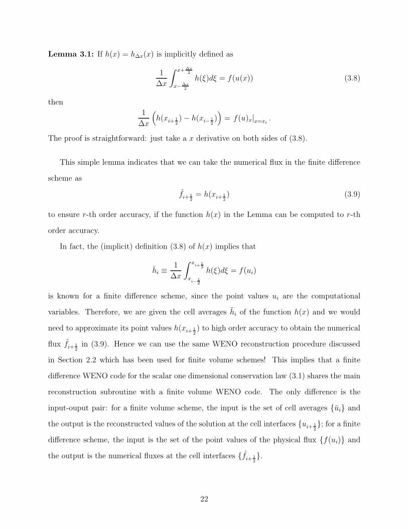
Lemma 3.1: If h(x) = h!x(x) is implicitly defined as
1
#x
" x+!x2
x!!x2
h($)d$ = f(u(x)) (3.8)
then1
#x
)h(xi+ 1
2) ! h(xi! 1
2)*
= f(u)x|x=xi.
The proof is straightforward: just take a x derivative on both sides of (3.8).
This simple lemma indicates that we can take the numerical flux in the finite di!erence
scheme as
fi+ 12
= h(xi+ 12) (3.9)
to ensure r-th order accuracy, if the function h(x) in the Lemma can be computed to r-th
order accuracy.
In fact, the (implicit) definition (3.8) of h(x) implies that
hi "1
#x
" xi+1
2
xi! 1
2
h($)d$ = f(ui)
is known for a finite di!erence scheme, since the point values ui are the computational
variables. Therefore, we are given the cell averages hi of the function h(x) and we would
need to approximate its point values h(xi+ 12) to high order accuracy to obtain the numerical
flux fi+ 12
in (3.9). Hence we can use the same WENO reconstruction procedure discussed
in Section 2.2 which has been used for finite volume schemes! This implies that a finite
di!erence WENO code for the scalar one dimensional conservation law (3.1) shares the main
reconstruction subroutine with a finite volume WENO code. The only di!erence is the
input-ouput pair: for a finite volume scheme, the input is the set of cell averages {ui} and
the output is the reconstructed values of the solution at the cell interfaces {ui+ 12}; for a finite
di!erence scheme, the input is the set of the point values of the physical flux {f(ui)} and
the output is the numerical fluxes at the cell interfaces {fi+ 12}.
22

For the purpose of stability, the finite di!erence procedure described above is applied to
f+(u) and f!(u) separately, where f±(u) correspond to a flux splitting
f(u) = f+(u) + f!(u) (3.10)
withd
duf+(u) $ 0,
d
duf!(u) # 0. (3.11)
The reconstruction for f+(u) uses a biased stencil with one more point to the left, and that
for f!(u) uses a biased stencil with one more point to the right, to obey correct upwinding.
We further require that f±(u) are as smooth functions of u as f(u). The most commonly
used flux splitting is the Lax-Friedrichs splitting
f±(u) =1
2(f(u) ± %u)
with
% = maxu
|f "(u)|.
However, other splittings can also be used. See, e.g. [76]. Notice that for any flux splitting
(3.10) satisfying (3.11), f(u!, u+) = f+(u!) + f!(u+) is a monotone flux.
Finally, we remark that the finite di!erence WENO scheme discussed in this section
can only be used on uniform or smooth meshes. Superficially, this is because Lemma 3.1
does not hold if #x is not a constant. A deeper reason is given in [106]. A conservative
finite di!erence scheme (3.6) with a local flux (3.7) cannot achieve higher than second order
accuracy on arbitrary non-uniform non-smooth meshes.
3.3 Comparison of finite volume and finite di!erence schemes
We can now summarize the main features of the finite volume and the finite di!erence WENO
schemes for solving the scalar one dimensional conservation law (3.1) as follows.
• A finite volume WENO scheme
1. is based on the cell averages {ui} and uses the integral form (3.3) of the PDE;
23

2. needs a WENO reconstruction described in Section 2.2 with the cell averages {ui}
as input and with the reconstructed point values {u±i+1/2} as output;
3. can use any monotone flux f(u!, u+);
4. can be applied to any meshes and does not need uniformity or smoothness of the
meshes.
• A finite di!erence WENO scheme
1. is based on the point values {ui}, and uses the original PDE form (3.1) directly;
2. needs a WENO reconstruction described in Section 2.2 with the point values of
the split fluxes {f±(ui)} as input and with the numerical fluxes {f±i+ 1
2
} as output;
3. can only use monotone fluxes which correspond to smooth flux splitting f(u) =
f+(u) + f!(u) satisfying (3.11);
4. can only be applied to uniform or smooth meshes.
Based on this comparison, we conclude that, for solving the one dimensional scalar con-
servation law (3.1), the cost of the finite volume and the finite di!erence WENO schemes
is the same (in fact they both involve the same WENO reconstruction procedure, the only
di!erence is the input-output pair). The finite volume scheme is more flexible in its ap-
plicability to any monotone fluxes and to any non-uniform non-smooth meshes. It would
seem that the finite volume scheme is clearly the winner. This conclusion is valid for all
one dimensional calculations, including the case of one dimensional systems. However, as
we will see in next subsection, the conclusion of this comparison changes dramatically for
multi-dimensional problems.
3.4 Multi-dimensional problems
We use a two dimensional scalar conservation law
ut + f(u)x + g(u)y = 0 (3.12)
24

to demonstrate finite volume and finite di!erence WENO schemes for multi-dimensional
problems. Furthermore, we assume that we have a tensor product mesh which is uniform
in both x and y. If we integrate the PDE (3.12) over a typical cell Iij " [xi! 12, xi+ 1
2] (
[yj! 12, yj+ 1
2], we obtain the integral form
d˜uij(t)
dt= ! 1
#x#y
.
/" y
j+ 12
yj! 1
2
f(u(xi+ 12, y, t))dy !
" yj+ 1
2
yj! 1
2
f(u(xi! 12, y, t))dy (3.13)
+
" xi+ 1
2
xi! 1
2
g(u(x, yj+ 12, t))dx !
" xi+1
2
xi! 1
2
g(u(x, yj+ 12, t))dx
0
1
where ˜u is the cell average
˜uij(t) "1
#x#y
" yj+ 1
2
yj! 1
2
" xi+1
2
xi!1
2
u(x, y, t)dxdy
In particular, our notation is that v stands for the cell average in x:
vij =1
#x
" xi+ 1
2
xi! 1
2
v(x, yj)dx
and v stands for the cell average in y:
vij =1
#y
" yj+ 1
2
yj! 1
2
v(xi, y)dy
We approximate the integral form (3.13) by a finite volume scheme
d˜uij(t)
dt= ! 1
#x(fi+ 1
2 ,j ! fi! 12 ,j) !
1
#y(gi,j+ 1
2! gi,j! 1
2)
where the numerical fluxes are given by
fi+ 12 ,j % ! 1
#y
" yj+ 1
2
yj! 1
2
f(u(xi+ 12, y, t))dy " fi+ 1
2 ,j
gi,j+ 12% ! 1
#x
" xi+1
2
xi! 1
2
g(u(x, yj+ 12, t))dx " gi,j+ 1
2
First, we look at the simple, linear constant coe"cient case
ut + aux + buy = 0
25

we would have
fi+ 12 ,j = aui+ 1
2 ,j, gi,j+ 12
= bui,j+ 12
Therefore we would only need to perform two one-dimensional WENO reconstructions
{˜uij} ) {ui+ 12 ,j} for fixed j
and
{˜uij} ) {ui,j+ 12} for fixed i
and the cost is the same as in the one-dimensional case per cell per direction.
However, if the PDE (3.12) is nonlinear, namely if f(u) and g(u) are nonlinear functions
of u, then f(u) *= 2f(u), hence we would need to perform two one-dimensional WENO
reconstructions and one numerical integration (typically via Gauss quadratures of su"cient
accuracy, which bears about the same cost as a reconstruction) to obtain the numerical flux
fi+ 12 ,j. Thus we would need to do
{˜uij} ) {ui+ 12 ,j} ) {ui+ 1
2 ,j+j!}!g
!=1 ) {fi+ 12 ,j}
where {j + j!}!g
!=1 are the Gaussian quadrature points for the interval [yj! 12, yj+ 1
2] with
su"ciently high order of accuracy. Likewise for gi,j+ 12. This is now about three times the
cost of the one-dimensional case per cell per direction. The situation will be much worse for
three dimensions.
On the other hand, a finite di!erence scheme approximates the PDE form (3.12) directly
and can proceed dimension by dimension. The scheme is
duij(t)
dt= ! 1
#x(fi+ 1
2 ,j ! fi! 12 ,j) !
1
#y(gi,j+ 1
2! gi,j! 1
2)
where the numerical flux fi+ 12,j can be computed from {uij} with fixed j in exactly the same
way as in the one dimensional case described in Section 3.2. Likewise for gi,j+ 12. Therefore,
the computational cost is exactly the same as in the one-dimensional case per point per
direction.
26

We can now conclude that in 2D, a finite volume scheme (of order of accuracy higher
than 2) is 2 to 5 times as expensive as a finite di!erence scheme of the same order of accuracy
using the same mesh and the same reconstruction procedure, depending on specific coding
and type of computers. This discrepancy in cost is even bigger for three dimensions. We
refer to [18] for a detailed comparison of multi-dimensional finite volume and finite di!erence
schemes in the context of ENO reconstructions. Notice that this di!erence between finite
volume and finite di!erence schemes is meaningful only for schemes of at least third order
accuracy. For first and second order schemes there is no need to distinguish between a finite
volume scheme and a finite di!erence scheme, since the cell average agrees with the value of
the function at the cell centroid to second order accuracy.
We should also mention again that finite volume schemes are more flexible than finite
di!erence schemes in terms of monotone fluxes and meshes. Conservative finite volume
schemes can be designed on arbitrary meshes. This is a more significant advantage in multi-
dimensions as one can design finite volume schemes on unstructured triangulations. However,
because of the significant cost advantage, conservative finite di!erence WENO schemes would
be preferable whenever the problem allows a uniform Cartesian or a smooth curvilinear mesh.
3.5 Further remarks
It should be remarked that the WENO reconstruction procedure, when the small parameter
# in (2.9) is chosen to be a small percentage of the size of typical ui under calculation, is
scale invariant. That is, the reconstruction does not change when the solution is amplified
by a constant, or when the mesh size #x changes. The WENO finite volume and finite
di!erence schemes are self-similar, that is, the numerical solution does not change if both
the spatial mesh size #x and the temporal mesh size #t change by the same factor and
& = !t!x does not change. Since the schemes are self-similar, we do not rely on explicit,
mesh size #x dependent thresholds to determine whether there are discontinuities in the
solution and their location. The numerical procedure automatically captures and handles
27

discontinuities or sharp gradient regions when they appear, so that accuracy and stability
are maintained. It is very important to have the numerical schemes satisfying these scale
invariant and self-similar properties for many applications.
Since WENO schemes have smooth numerical fluxes and are dissipative, they can be
shown to converge with high order accuracy using Strang’s framework [150] when the so-
lution of the PDE is smooth [76]. When the solution of the PDE becomes discontinuous,
there is no general proof of stability and convergence for high order WENO schemes solv-
ing conservation laws. However, in applications WENO schemes perform well in stability
and resolution. As to numerically observed order of accuracy in smooth regions of a dis-
continuous solution, for scalar problems the full designed order of accuracy of the WENO
scheme is achieved if we measure the error away from the discontinuity. For systems, be-
cause characteristics belonging to di!erent fields than that of the discontinuity may cross
the discontinuity and carry the numerical error at the discontinuity into smooth regions,
point-wise errors in smooth regions of a high order WENO scheme may fail to achieve the
designed order of accuracy, unless a sub-cell resolution technique [62] is used in the shocked
cell. We demonstrate this phenomenon by a nozzle flow simulation using a fourth order
residual distribution WENO scheme in [24]. In Figure 3.1, we observe good resolution of
the WENO numerical solution in comparison with the exact solution of the nonlinear Euler
system with source terms. In Table 3.1, we observe that the designed fourth order accuracy
is achieved for both upstream and downstream of the shock if a sub-cell integration technique
is applied in the shocked cell, while the accuracy downstream of the shock has lower than
the designed fourth order accuracy if no special treatment is performed in the shocked cell.
Nevertheless, even if the order of accuracy for the pointwise errors downstream of the shock
may degenerate for a higher order WENO scheme, the magnitude of the errors is typically
still much smaller than that of a lower order scheme on the same mesh. In practice, this is
the advantage that we rely on when we use high order WENO schemes to solve complicated
nonlinear systems with both shocks and smooth structures in the solutions.
28

x
density
0 0.2 0.4 0.6 0.8 1
0.5
0.6
0.7
0.8
0.9exactnumerical
x
pressure
0 0.2 0.4 0.6 0.8 1
0.4
0.5
0.6
0.7
0.8
0.9
exactnumerical
Figure 3.1: Fourth order residual distribution WENO scheme for the nozzle flow problem.Non-smooth mesh with 81 cells. Solid lines: exact solution; symbols: numerical solution.Left: density. Right: pressure.
Even though the pointwise errors for a high order scheme solving discontinuous solutions
of a hyperbolic system may show a low order of accuracy, it is well known [83, 103] that the
designed high order accuracy is maintained in integrated quantities of the numerical solution
such as moments against smooth functions, if the scheme and the PDE are both linear. With
this information, we can post-process the numerical solution to obtain the designed order
of accuracy also for point values [52]. This is a strong theoretical justification to use high
order schemes even for discontinuous solutions. Recently, [54] has given numerical evidence
to indicate that such high order information may also be available for high order WENO
schemes in solving nonlinear systems.
For systems of conservation laws, the WENO schemes have the same structure as those
for the scalar cases discussed in the previous subsections. A monotone flux is replaced by
an exact or approximate Riemann solver, see, e.g. [156]. The WENO reconstruction can be
performed either component-wise, or in local characteristic directions. Usually, component-
wise reconstruction produces satisfactory results for schemes up to third order accuracy,
while characteristic reconstruction produces better non-oscillatory results for higher order
accuracy, albeit with an increased computational cost. Details about the local characteristic
29

Table 3.1: Fourth order residual distribution WENO scheme for the nozzle flow problem.Errors outside three cells around the shock and numerical orders of accuracy for the density' on non-smooth meshes with N cells.
sub-cell separate integrations in the shocked cellbefore shock after shock
N L1 error order L$ error order L1 error order L$ error order21 1.36E-07 - 7.09E-07 - 7.58E-06 - 3.35E-05 -41 1.44E-08 3.23 6.13E-08 3.53 5.08E-07 3.90 2.19E-06 3.9381 1.28E-09 3.49 4.85E-09 3.66 1.67E-08 4.93 6.61E-08 5.05161 8.34E-11 3.94 3.11E-10 3.96 7.72E-10 4.43 3.00E-09 4.46321 5.41E-12 3.95 2.00E-11 3.96 3.65E-11 4.40 1.36E-10 4.46641 2.22E-13 4.60 1.20E-12 4.05 1.75E-12 4.38 4.92E-12 4.80
regular integration in the shocked cellbefore shock after shock
N L1 error order L$ error order L1 error order L$ error order21 1.36E-07 - 7.09E-07 - 1.75E-05 - 6.42E-05 -41 1.44E-08 3.24 6.13E-08 3.53 4.38E-06 1.99 1.42E-05 2.1881 1.28E-09 3.49 4.85E-09 3.66 1.11E-06 1.98 3.37E-06 2.07161 8.34E-11 3.94 3.11E-10 3.96 2.34E-07 2.25 7.29E-07 2.21321 5.41E-12 3.95 2.00E-11 3.96 5.81E-08 2.01 1.77E-07 2.04641 2.22E-13 4.61 1.22E-12 4.04 8.15E-09 2.83 2.52E-08 2.81
decomposition procedure can be found in many papers, e.g. [64, 146, 148].
When designing numerical schemes to solve hyperbolic systems with source terms
ut + f(u)x = g(u, x), (3.14)
which are also called balance laws, it is a challenge to have the scheme maintaining specific
equilibria, that is, steady state solutions satisfying
f(u)x = g(u, x)
exactly. This is because such equilibria are usually not constant or polynomial functions, so
the truncation error of most schemes will not be exactly zero for such equilibria. A scheme
which can maintain such equilibria is referred to as a well balanced scheme. The main
advantage of well balanced schemes, especially when they are also high order accurate for
non-equilibrium solutions of (3.14), is that they can be used to resolve small perturbations
30

of such equilibria, such as the small amplitude water waves from still water, very accurately
without an excessively refined mesh. High order finite di!erence and finite volume WENO
schemes which are well balanced for the still water solution of the shallow water equations,
and a more general class of balance laws, are designed in [110, 158, 161, 162, 163, 164]. High
order well balanced finite di!erence WENO schemes for solving the hyperbolic models for
chemosensitive movement are designed in [46]. High order finite volume WENO schemes
which are well balanced for the moving steady water of the shallow water equations, which
are much more di"cult to construct, are designed in [111]. As an example, in Figure 3.2 we
plot the water surface from a small perturbation (the perturbation amplitude is 1% of the still
water height) for later time, simulated by a fifth order well balanced WENO scheme [161].
We can see clearly that the detailed structure of the evolution of such a small perturbation is
resolved well even with the relatively coarse mesh of 200( 100 points. If a regular, non-well
balanced WENO scheme is used, much smaller mesh sizes are needed to resolve the evolution
of such small perturbations.
In [136], a modification to the fifth order WENO scheme, termed power WENO scheme,
is developed based on an extended class of limiters. Comparison with the standard WENO
scheme is made with extensive numerical examples.
In our previous discussion, we have not paid attention to boundary conditions and have
assumed the problem has no boundary (compactly supported data or periodic boundary
conditions). In practice, of course we would need to deal with various physical boundary
conditions. WENO schemes have been used for problems with di!erent boundary conditions
such as reflective (solid wall), symmetry (such as the axis in an axis-symmetric setting),
inflow and outflow types. A general strategy is to define accurate ghost point values based
on the specific type of boundary conditions, coupled with local characteristic decompositions.
One-sided WENO approximations or reconstructions, which avoid using information from
outside the computational domain, may also be used [135, 24].
The finite volume scheme (3.4), when discretized in time, can also be defined on a stag-
31

0 0.5 1 1.5 20
0.2
0.4
0.6
0.8
1surface level at time t=0.12
0 0.5 1 1.5 20
0.2
0.4
0.6
0.8
1surface level at time t=0.12
0 0.5 1 1.5 20
0.2
0.4
0.6
0.8
1Surface level at time t=0.24
0 0.5 1 1.5 20
0.2
0.4
0.6
0.8
1surface level at time t=0.24
0 0.5 1 1.5 20
0.2
0.4
0.6
0.8
1surface level at time t=0.36
0 0.5 1 1.5 20
0.2
0.4
0.6
0.8
1surface level at time t=0.36
0 0.5 1 1.5 20
0.2
0.4
0.6
0.8
1surface level at time t=0.48
0 0.5 1 1.5 20
0.2
0.4
0.6
0.8
1surface level at time t=0.48
0 0.5 1 1.5 20
0.2
0.4
0.6
0.8
1surface level at time t=0.6
0 0.5 1 1.5 20
0.2
0.4
0.6
0.8
1surface level at time t=0.6
Figure 3.2: Two dimensional shallow water equation. Small (1%) perturbation from stillwater. Well balanced fifth order finite di!erence WENO scheme [161]. The contours of thewater surface level. 30 uniformly spaced contour lines. From top to bottom: at time t = 0.12from 0.999703 to 1.00629; at time t = 0.24 from 0.994836 to 1.01604; at time t = 0.36 from0.988582 to 1.0117; at time t = 0.48 from 0.990344 to 1.00497; and at time t = 0.6 from0.995065 to 1.0056. Left: results with a 200 ( 100 uniform mesh. Right: results with a600 ( 300 uniform mesh.
32

gered mesh, resulting in a class of central schemes [109]. An advantage of such central
schemes is that the numerical flux is computed in the smooth part of the reconstructed
function, hence there is no need to use explicitly a monotone flux for the scalar case or a
Riemann solver for the system case. WENO schemes based on the central scheme frame-
work have been constructed in the literature, e.g. in [88, 89, 90, 124]. It seems that the
central scheme framework allows the component-wise WENO reconstruction procedure to
be used for less oscillatory results for third or even fourth order schemes, however for very
high order central WENO schemes, characteristic WENO reconstruction is still necessary to
obtain stable results [124]. A detailed assessment of component-wise versus characteristic
reconstructions in the context of central WENO schemes is given in [124].
Finite volume WENO schemes on multi-dimensional structured meshes are straightfor-
ward to design [139]. Finite volume WENO schemes on two dimensional unstructured meshes
are designed in [48, 71, 139, 42, 43]. For three dimensions, finite volume WENO schemes
on unstructured meshes are designed in [42, 43, 184]. As we mentioned in Section 2.3, the
WENO schemes in [48, 42, 43] choose the linear weights not to increase the order of accu-
racy of the approximation in each sub-stencil. Therefore these schemes do not achieve the
optimal attainable order of accuracy for their stencil. However these schemes are easier to
design since the linear weights can be chosen to be arbitrary positive constants, or to fit
other constraints such as having larger linear weights for the more symmetric sub-stencils.
The WENO schemes in [71, 139, 184] follow the traditional WENO procedure to obtain
approximations on the larger stencil which are of higher order accuracy than that on each
sub-stencil. Unfortunately, such schemes are very di"cult to construct on unstructured
meshes as the optimal linear weights depends on the local mesh distribution.
In [135], a multi-domain finite di!erence WENO scheme is designed. The computational
domain can then be generalized to any region which can be covered by overlapping patches
where for each patch a uniform Cartesian or a smooth curvilinear mesh suitable for a finite
di!erence WENO scheme can be used. Information is transferred between patches via high
33

order interpolation. This multi-domain finite di!erence WENO scheme can be used in many
practical situations, such as flow passing a wedge, with the cost of a finite di!erence scheme
which is much smaller than that of a finite volume scheme. This scheme is used in [80] to
study shock mitigation and drag reduction by pulsed energy lines.
Another attempt to expand the usability of the finite di!erence WENO method without
increasing its cost is the design of residual distribution type finite di!erence WENO schemes
for steady state conservation laws and convection dominated convection di!usion equations
in [24, 25]. These schemes can be used on arbitrary non-smooth tensor product curvilinear
meshes, are conservative, and have the same cost as the usual conservative finite di!erence
schemes for two dimensional problems.
One di"culty of numerical solutions for conservation laws is that contact discontinuities,
i.e. the discontinuities belonging to the characteristic field satisfying &"(u) · r(u) " 0 where
&(u) is an eigenvalue and r(u) the corresponding eigenvector of the Jacobian f "(u) of the
conservation law (3.1), are much more di"cult to resolve sharply than shocks. This is
because the characteristics are parallel to the discontinuity for a contact discontinuity, while
they converge into the discontinuity for a shock, see Figure 3.3. Therefore, a numerical shock
is usually stable with a fixed number of transition points for long time simulation, while a
numerical contact discontinuity may progressively become wider for longer time simulation.
Strategies to improve the resolution of contact discontinuities for high order WENO schemes
include the artificial compressibility method [169, 76], sub-cell resolution [62, 76], and the
anti-di!usive flux correction method [40, 165]. We will use an example of shallow water
with transport of pollutant [167] to demonstrate the performance of the anti-di!usive flux
correction technique for high order WENO schemes developed in [165]. In Figure 3.4, we
compare the performance of the regular fifth order WENO scheme and the anti-di!usive
flux corrected fifth order WENO scheme for the resolution of pollutant. Comparing with
the reference solution at the bottom of Figure 3.4, which is computed with the regular fifth
order WENO scheme with an extremely refined mesh and can be considered as an exact
34

solution, the quality of the anti-di!usive WENO scheme is much better than that of the
regular WENO scheme on the relatively coarse mesh with 300 ( 100 points.
x
t
x
t
Figure 3.3: Characteristics. Left: contact discontinuity; right: shock.
For convection dominated convection di!usion equations, for example the Navier-Stokes
equations with high Reynolds numbers, the WENO schemes discussed in previous subsec-
tions for conservation laws can be easily generalized. We can either use central di!erence
approximations to the second derivative viscous terms of comparable order of accuracy, or
absorb the evaluation of the viscous terms into the numerical fluxes by first computing an
approximation to the first derivatives of the solution at cell interfaces to the desired order
of accuracy. We refer to, e.g., [182, 185, 179, 180] for more details.
Since WENO schemes are explicit schemes, they can be implemented easily on massively
parallel platforms. Large scale results obtained in, e.g. [45, 179, 180, 182, 185] are obtained by
parallel WENO codes. The parallel e"ciency of the high order WENO schemes is excellent.
4 WENO schemes for Hamilton-Jacobi equations
WENO schemes can be used also to solve PDEs which are not hyperbolic conservation laws.
In this section we describe such an example. We consider WENO schemes for solving the
following Hamilton-Jacobi equations
(t + H((x1, ...,(xd) = 0, ((x, 0) = (0(x), (4.1)
35

where the Hamiltonian H is a (usually nonlinear) function which is at least Lipschitz contin-
uous. H could also depend on (, x and t in some applications, however the main di"culty
for numerical solutions is the nonlinear dependency of H on the gradient of (.
Hamilton-Jacobi equations appear often in many applications. One important application
of Hamilton-Jacobi equations is the area of image processing and computer vision. Other
application areas include, e.g. control and di!erential games.
The main di"culty in the numerical solutions of the Hamilton-Jacobi equation (4.1) is
that global C1 solution does not exist in the generic situation, regardless of the smoothness
of the initial condition (0(x). Singularities in the form of discontinuities in the derivatives
of ( would appear at a finite time in most situations, thus the solutions would be Lipschitz
continuous but no longer C1. In fact, at least in the one dimensional case, there is an
equivalence between the Hamilton-Jacobi equation
(t + H((x) = 0, ((x, 0) = (0(x) (4.2)
and the hyperbolic conservation law
ut + H(u)x = 0, u(x, 0) = u0(x) (4.3)
if we identify u = (x. As we have seen in Section 3, singularities for the conservation law
(4.3) are in the form of discontinuities in the solution u, thus u is bounded, with a bounded
total variation, but is not continuous. The results for the conservation law (4.3) can be
directly translated to that for the Hamilton-Jacobi equation (4.2) by integrating u once.
Discontinuities in u then become discontinuities for the derivative of (.
For the one dimensional Hamilton-Jacobi equation (4.2), or for the multi-dimensional
Hamilton-Jacobi equation (4.1) on a tensor product mesh, the WENO finite di!erence scheme
[75] can be easily designed. We will use the one dimensional version (4.2) to demonstrate
the idea. The WENO scheme in this case evolves the point values of the solution (i in the
following wayd
dt(i + H(u!
i , u+i ) = 0 (4.4)
36

where H(u!, u+) is a monotone Hamiltonian, namely it is non-decreasing in its first argument
u! and non-increasing in its second argument u+, or symbolically H(&, '); it is consistent
with the physical Hamiltonian H(u), i.e. H(u, u) = H(u); and it is Lipschitz continuous with
respect to both arguments u! and u+. Monotone Hamiltonians can also be defined for multi-
dimensional cases (4.1). We refer to, e.g. [114], for examples of monotone Hamiltonians in
one- and multi-dimensional cases. The values u±i in (4.4) are WENO approximations to the
derivatives of ( at the point xi with a stencil one point biased to the left and one point
biased to the right, respectively, described in Section 2.3. For example, a fifth order WENO
scheme [75] uses the following stencil to approximate u!i :
S = {xi!3, xi!2, xi!1, xi, xi+1, xi+2}.
This stencil is the union of the following three sub-stencils
S1 = {xi!3, xi!2, xi!1, xi}, S2 = {xi!2, xi!1, xi, xi+1}, S3 = {xi!1, xi, xi+1, xi+2}
The fifth order approximation u!i is, as usual, a convex combination of the three third order
approximations to (x at x = xi based on the three sub-stencils S1, S2 and S3 respectively.
Time discretization to the semi-discrete scheme (4.4) can again be based on the TVD Runge-
Kutta time discretizations such as (3.5).
Unlike the case of conservation laws in Section 3, for the Hamilton-Jacobi equation (4.4)
there is no finite volume scheme, and the finite di!erence scheme we described above does
not have the restriction of uniform or smooth meshes. This finite di!erence scheme can
be used on any mesh, smooth or not. For the multi-dimensional case (4.1), as long as we
have a tensor product mesh, the finite di!erence WENO scheme can be trivially generalized,
by simply computing approximations to the derivatives dimension by dimension. Thus the
approximation to u = (x is obtained by the one dimensional procedure described above
along the x direction with y fixed, and the approximation to v = (y is obtained by the same
one dimensional procedure along the y direction with x fixed. WENO schemes can also be
designed based on the central scheme framework, see, e.g. [8, 149]. However, a high order
37

WENO scheme to solve the multi-dimensional case (4.1) on unstructured meshes is much
more involved. We refer to [183] for the details of high order WENO schemes solving two
dimensional Hamilton-Jacobi equations on general triangulations; see also [87].
WENO schemes have been used widely in solving Hamilton-Jacobi equations from level
sets [113]. For some of these application problems, for example for the problem of reinitial-
ization of the signed distance function [152], one must solve steady state Hamilton-Jacobi
equations repeatedly. One of the e"cient methods to solve the steady state Hamilton-Jacobi
equations is the so-called fast sweeping method. For high order WENO schemes, fast sweep-
ing methods have been developed recently in [186].
Similar to the di"culty associated with the resolution of contact discontinuities in con-
servation laws, it is also di"cult to resolve corners (discontinuities in the derivative of the
solution) corresponding to a linearly degenerated Hamilton-Jacobi equation. In [166], the
anti-di!usive flux correction technique in [165] for conservation laws is generalized to high
order WENO schemes for solving Hamilton-Jacobi equations, to sharpen such corners. Nu-
merical results in [166] demonstrate the good performance of this approach.
Finally, we mention that the convergence of a class of semi-Lagrangian large time step
schemes, based on a WENO interpolation with the order of accuracy as high as 9, is proved
in [13] for solving general viscosity solutions of convex Hamilton-Jacobi equations. This is
the best theoretical convergence result obtained so far involving WENO schemes.
38

1 2
0.1
0.2
0.3
0.4
0.5
0.6
0.7
0.8
0.9
1
1 2
0.1
0.2
0.3
0.4
0.5
0.6
0.7
0.8
0.9
1
1 2
0.1
0.2
0.3
0.4
0.5
0.6
0.7
0.8
0.9
1
1 2
0.1
0.2
0.3
0.4
0.5
0.6
0.7
0.8
0.9
1
Figure 3.4: Shallow water equation coupled with the transport of pollutant. 300 ( 100uniform mesh. Contours of the pollutant T . Top: the initial pollutant. Second: pollutantobtained by the regular fifth order WENO. Third: pollutant obtained by the anti-di!usivefifth order WENO. Bottom: reference solution obtained by 1500 ( 500 uniform mesh withregular fifth order WENO.
39

5 Relationship and comparison with other high orderschemes
In this section we would like to briefly describe a few competitive types of numerical methods
for solving convection dominated problems. Rather than surveying the details of these
methods, we emphasize e!orts in combining the advantages of these methods and the WENO
procedure. Comparisons of some of these schemes with WENO schemes can be found in
[187, 144].
5.1 Discontinuous Galerkin method
Discontinuous Galerkin methods are a class of finite element methods that have gained a lot
of popularity in recent years, e.g. [31, 32, 37]. For our purpose, the discontinuous Galerkin
methods can also be viewed as a generalized finite volume method for solving conservation
laws. For the one dimensional conservation law (3.1), instead of integrating it in the cell
Ii = (xi! 12, xi+ 1
2) to obtain the integral form (3.3), which forms the basis of the finite volume
scheme (3.4), we multiply the PDE (3.1) by a test function v and then integrate it in the
cell Ii to obtain, after an integration by parts
" xi+1
2
xi! 1
2
utvdx !" x
i+12
xi!1
2
f(u)vxdx + f(ui+ 12)vi+ 1
2! f(ui! 1
2)vi! 1
2= 0 (5.1)
To convert (5.1), which is satisfied by the exact solution u of the PDE (3.1) and any test
function v, to a discontinuous Galerkin scheme, we would like to replace u and v by functions
in a finite dimensional piecewise polynomial space V!x defined by
V!x =3v : v|Ij + P k(Ij), j = 1, · · · , N
4
with P k(Ij) denoting the set of polynomials of degree up to k defined on the cell Ij. However,
the boundary terms ui+ 12
and vi+ 12
etc. would not be well defined for functions in V!x, since
they are discontinuous exactly at such cell interfaces. If we take v = 1Ii to be the indicator
function of cell Ii, that is, v(x) = 1 when x + Ii and v(x) = 0 otherwise, then (5.1) becomes
40

the integral form (3.3) which forms the basis of the finite volume scheme (3.4). We hope that
the discontinuous Galerkin scheme would be of the same form as the finite volume scheme
(3.4) for this choice of v, which motivates the choice of the interface values as follows:
1. f(ui+ 12) is replaced by a single valued monotone numerical flux fi+ 1
2= f(u!
i+ 12
, u+i+ 1
2
)
which depends on both the left and right values of u at the cell interface xi+ 12. Naturally,
f(ui! 12) is replaced by f(u!
i! 12
, u+i! 1
2
).
2. The test function v is replaced by its values inside the relevant cell, that is, by v!i+ 1
2
at
the right boundary of cell Ii and by v+i! 1
2at the left boundary of cell Ii.
Thus the discontinuous Galerkin scheme is: find u + V!x such that
" xi+1
2
xi! 1
2
utvdx !" x
i+12
xi!1
2
f(u)vxdx + fi+ 12v!
i+ 12! fi! 1
2v+
i! 12
= 0 (5.2)
for all v + V!x.
Notice that by taking the test function v = 1Ii + V!x we obtain the same identity as
the finite volume scheme (3.4). Therefore we may claim that the discontinuous Galerkin
scheme (5.2) is a generalized finite volume scheme. However, an essential di!erence between
the finite volume scheme (3.4) and the discontinuous Galerkin scheme (5.2) is that the finite
volume scheme evolves only one piece of information per cell, namely the cell average ui. If
higher order point values u±i+ 1
2
are needed at the cell interfaces, they will be reconstructed by
the WENO procedure. On the other hand, the discontinuous Galerkin scheme evolves the
whole polynomial per cell Ii (if the polynomial is of degree k then k+1 pieces of information
is evolved per cell). This increases the storage and computational cost for the evolution,
however it then eliminates the cost of reconstruction completely.
Since the WENO procedure is only applied at the reconstruction stage of the finite volume
scheme, it cannot be directly used within the framework of a discontinuous Galerkin scheme.
Therefore, discontinuous Galerkin schemes rely on limiters to control spurious oscillations.
See, e.g. [28, 27, 30].
41

The discontinuous Galerkin methods are more flexible than the finite volume WENO
schemes for solving conservation laws on multi-dimensional unstructured meshes. This is
because the discontinuous Galerkin methods do not involve the reconstruction procedure,
which tends to be very complicated for unstructured meshes. However, the discontinuous
Galerkin methods are less robust in dealing with solutions with strong shocks. This is because
the state of the art for limiters is less advanced than the WENO procedure in controlling
spurious oscillations without a!ecting accuracy for smooth structures.
Recently, e!orts have been made in the following two directions to combine the advantages
of WENO and discontinuous Galerkin schemes:
1. The design of Hermite type WENO schemes. These are schemes between the finite
volume WENO scheme, which evolves only one piece of information per cell, and the
discontinuous Galerkin scheme, which evolves k + 1 pieces of information per cell for a
(k+1)-th order method in one dimension using piecewise polynomials of degree k. The
Hermite WENO schemes designed in [126, 129, 130] evolve a linear function per cell
(hence they evolve 2 pieces of information per cell in one dimension) and reconstruct
the necessary point values to higher order accuracy when necessary. Because each cell
contains more than one degrees of freedom, the reconstruction would involve a narrower
stencil for the same order of accuracy, resulting in more compact WENO schemes.
2. The design of WENO limiters for the discontinuous Galerkin schemes. The idea is to
first identify the so-called “troubled cells”, then retain only the cell average information
in such cells for the purpose of conservation, and use the WENO procedure to recon-
struct the higher order moments of the polynomials in such cells using the information
from neighboring cells. Both the traditional WENO reconstruction technique and the
Hermite WENO reconstruction technique (which is more desirable since it involves a
narrower stencil) can be used. This approach has been pursued in [127, 126, 129]. The
issue of e!ective “troubled cell” indicators has been addressed in [128].
42

5.2 Compact schemes
Compact schemes are finite di!erence schemes where the derivatives are approximated not
by polynomial operators but by rational function operators on the discrete solutions. For
example, a fourth order central compact approximation to the first derivative is given by
1
6((ux)i!1 + 4(ux)i + (ux)i+1) =
1
2#x(ui+1 ! ui!1) (5.3)
Clearly, a tridiagonal linear solver is needed to obtain the approximation (ux)i for all i from
(5.3). From this point of view, compact approximations to derivatives are not really compact,
since the approximation to (ux)i involves contributions from all the grid values uj. We refer
to, e.g. [70, 85] for the general discussion of compact schemes. Upwind (rather than central)
compact schemes are developed in [29].
The main advantage of compact schemes is that they have better resolution power for
high frequency waves than the usual finite di!erence schemes of the same order of accuracy.
Therefore, they are especially suitable for problems involving long time evolution of waves,
such as turbulence simulations [85].
E!orts have been made in the literature to develop hybrid compact WENO schemes.
In [79], a compact WENO scheme is designed where the WENO procedure is used on the
explicit part of the scheme (the right hand side of (5.3)). In [115], a hybrid compact-WENO
scheme is developed to solve shock turbulence interaction problems. A shock detector is
used to find regions where the WENO approximation is used instead of the usual compact
di!erence approximation. In [39], the WENO procedure is used to build nonlinear WENO
compact schemes.
5.3 Spectral method
For smooth problems in regular geometry, the spectral method [51, 12] is the most powerful
method to obtain accurate results, especially for long time wave propagation problems.
Fourier or Chebyshev spectral methods are also very e"cient because of the Fast Fourier
43

Transforms. However, it is a challenge to design stable spectral schemes for solving convection
dominated problems which have sharp gradient regions or shocks. Even though spectral
methods with a carefully designed application of filters can produce very good results for
shock wave calculations [41], such methods are not robust, in the sense that the application
of filters requires experience in order to maintain stability without destroying accuracy.
E!orts have been made in the literature to develop hybrid spectral WENO schemes. In
[35, 34], a hybrid spectral WENO method, using the WENO procedure near strong shocks
and spectral procedure elsewhere, is developed and demonstrated to give good numerical
results for a few quite demanding test problems.
5.4 Wavelets and multi-resolution methods
Wavelets and multi-resolution methods are powerful frameworks to solve multi-scale prob-
lems containing a wide range of physical scales. In applications to solve convection domi-
nated PDEs, the multi-resolution framework of Harten [63] is particularly attractive, since
it utilizes the essential ideas of wavelets in their e!ective multi-resolution decomposition
in combination with features in conservative schemes for hyperbolic conservation laws rely-
ing on high order reconstruction. There have been numerous works since then combining
Harten’s multi-resolution framework with high order, high resolution schemes, see for ex-
ample [7, 23]. Recently, this multi-resolution framework has also been combined with the
WENO procedure in [9] to produce an adaptive multiresolution WENO scheme for solving
conservation laws.
5.5 Dispersion optimized finite di!erence schemes
For application problems in which waves must propagate over a long time with a relatively
coarse mesh (that is, the number of grid points per wave is not large), such as problems in
aeroacoustics and electro-magnetism, it is important to maintain the phase accuracy of the
waves to the best extent possible. Spectral methods are the best choice to maintain such
phase accuracy. Compact schemes discussed in Section 5.2 are also good choices. If one must
44

use explicit finite di!erence schemes, then there is a systematic approach [153] to modify the
coe"cients of the finite di!erence approximation, with the objective of increasing the phase
resolution (dispersion relation) at the price of lowering the order of accuracy for the same
stencil. Even though such dispersion optimized finite di!erence schemes are less accurate
for asymptotically small mesh sizes (that is, when the number of points per wave is large),
they are better than the usual finite di!erence schemes on the same stencil for marginally
resolved waves (that is, when the number of points per wave is small).
Even though WENO schemes are nonlinear, they can also be adapted by such dispersion
optimized technique to enhance their resolution power for marginally resolved waves. E!orts
are made in the literature [98, 119, 159, 105] to design such dispersion optimized WENO
schemes and to apply them for turbulence simulations.
6 Applications
The WENO schemes discussed in previous sections have been used in many physical and
engineering applications. In this section we briefly summarize some of these applications
with the objective of giving a glimpse of the diversity of possible applications of the WENO
methodology, rather than providing an exhausting list. Most of these applications have a
common feature: they are solving for solutions with both discontinuities or sharp gradient
regions and complicated smooth region structures.
6.1 Computational fluid dynamics
The largest application area of WENO schemes is the area of computational fluid dynamics
(CFD). Besides the applications already mentioned in previous sections, we mention as
additional examples the following representative works.
1. Shock vortex interaction is an important physical process for sound generation, and
it is a simple model for shock turbulence interaction. This problem has complicated
solutions where shocks of various strengths and vorticity flows co-exist, which makes it
45

ideal to be simulated by high order WENO schemes. Many papers in the literature use
WENO scheme to study the details of shock vortex interactions in di!erent physical
setup and regimes, for example [57, 116, 117, 131, 179, 180]. See also related work
in blast wave/vortex interaction and sound generation in [21]; shock wave-thermal
inhomogeneity interactions in [58]; reflected shock/vortex interaction near an open-
ended duct in [93]; and shock/vortex interactions induced by blast waves in [94]. As an
example of shock vortex interaction, in Figure 6.1 we plot the shadowgraphs (contours
of ,2' where ' is the density) of an oblique Mach 1.2 shock with a strong colliding
vortex pair simulated by the fifth order WENO scheme for the compressible Navier-
Stokes equations [180]. We can see clearly that complicated flow structure from the
shock vortex interaction is resolved well by the fifth order WENO scheme.
2. High speed and turbulent flows typically contain both strong shocks and complicated
flow structures, making WENO schemes good simulation tools for them. Supersonic
jet and shear layers are studied in [22]. Turbulent flows in high-speed aerodynamics are
studied in [60]. Turbulence spectra characteristics for direct and large eddy simulations
are studied in [82]. Hypersonic aerodynamic heating prediction is made in [84]. The
starting process in a supersonic nozzle is studied in [108]. Direct numerical simulation
and analysis of a spatially evolving supersonic turbulent boundary layer at M=2.25
are performed in [118]. Instability wave generation and propagation in supersonic
boundary layers are studied in [78]. Large eddy simulation of the shock wave and
boundary layer interaction is performed using the hybrid compact/WENO scheme
in [154]. Implicit WENO schemes for the compressible and incompressible Navier-
Stokes equations are developed in [170, 171] and used to perform the three-dimensional
wing flow computations in [172]. Computation of supersonic turbulent flowfield with
transverse injection is performed in [151]. The stochastic piston problem is studied in
[97]. Nearly-incompressible, inviscid Taylor-Green vortex flow is studied in [145].
46

(a) t = 5.0 (b) t = 7.0
(c) t = 9.0 (d) t = 13.0
Figure 6.1: Fifth order WENO simulation of the evolution of an oblique shock and a collidingvortex pair interaction [180]. Shock Mach number Ms = 1.2, vortex Mach number M" = 0.8,and angle of the oblique shock wave % = 45%.
47

3. Reacting flows, detonations, and flames contain multiple scales in the solution together
with shocks, making the numerical simulation of them very di"cult. WENO schemes
have been successfully used for such simulations. Reacting flows with complicated so-
lution structure are studied in [2]. Pulse detonation engine phenomena are studied in
[67]. A very accurate simulation of pulsating one-dimensional detonations is performed
in [68, 69]. The structure and evolution of a two-dimensional H-2/O-2/Ar cellular det-
onation are studied in [72]. A unified model for the prediction of laminar flame transfer
functions is built, and comparisons are made between conical and V-flame dynamics
in [134]. Modeling tools for the prediction of premixed flame transfer functions are
studied in [133].
4. An interesting application of shock mitigation and drag reduction by pulsed energy
lines for supersonic flows past a wedge is studied in [80] using the multi-domain finite
di!erence WENO scheme developed in [135]. The simulation results indicate a saving
of energy (energy gained is larger than energy spent to generate the pulsed energy
lines) for all studied configurations.
5. A WENO finite di!erence scheme for solving the magnetohydrodynamics (MHD) flows
is developed in [77]. This code is used in, e.g. [160] to study the dynamical evolution
of coherent structures in intermittent two-dimensional MHD turbulence.
6. Real gas computation using an energy relaxation method is performed in [107]. Com-
pressible multicomponent flows are simulated in [102, 104]. A pseudocompressibility
method for the numerical simulation of incompressible multifluid flows is developed in
[112]. Modeling and simulation for a particle-fluid two phase flow problem are studied
in [177].
7. Hydrodynamic and quasi-neutral approximations for collisionless two-species plasmas
are performed in [81]. E!ects of shock waves on Rayleigh-Taylor instability are studied
in [185]. An example of the Rayleigh-Taylor instability with or without shock waves is
48

X
Y
0 0.2 0.40
0.1
0.2
0.3
0.4
0.5
0.6
0.7
0.8
0.9
1
Density
1.831.701.581.451.321.191.070.940.81
No shock, T=6.0
X
Y
0 0.2 0.4-17.5
-17
-16.5
-16
Density
8.027.486.946.415.875.334.794.263.72
Mach 12 shock, T=3.0
X
Y
0 0.2 0.411
11.5
12
12.5
Density
6.446.145.835.535.224.924.614.314.00
Mach 12 shock, T=3.0shock hits tail
(a) (b) (c)
Figure 6.2: Ninth order WENO simulation of the Rayleigh-Taylor instability with or withoutshock waves [185]. Left (a): the Rayleigh-Taylor flow at T = 6.0; middle (b): Mach 12 shockhitting the Rayleigh-Taylor interface from the top, T = 3.0; right (c): Mach 12 shock hittingthe Rayleigh-Taylor interface from the bottom, T = 3.0. Density '.
shown in Figure 6.2, in which a Rayleigh-Taylor flow (left picture) is compared with
the flow of a Mach 12 shock hitting the Rayleigh-Taylor interface from the top (middle
picture) and from the bottom (right picture) [185]. The simulation is performed by a
ninth order WENO scheme, which seems to resolve the complicated flow structures in
the presence of strong shocks very well. We can clearly observe that the shock waves
do speed up the transition of the Rayleigh-Taylor flow to full instability in each case.
8. Shallow water equations and sediment transport equations are studied in [36]. Two-
dimensional shallow water equations are simulated by composite schemes (for which
WENO is a component) in [100], see also [99]. Underwater blast-wave focusing is
studied in [92]. Non-breaking and breaking solitary wave run-up is studied in [91]. See
also [158, 161, 163, 164] for well balanced high order WENO schemes for the shallow
water equations.
49

9. Numerical simulation of interphase mass transfer with the level set approach is per-
formed in [168]. Migrating and dissolving liquid drops are studied in [5, 6]. For flows
in liquid helium, nonlinear e!ects and shock formation in the focusing of a spherical
acoustic wave are studied in [3].
10. A WENO scheme is designed in [16] for the Lifshitz-Slyozov system, which models the
formation of a new phase in solid mechanics. This is not exactly fluid mechanics but
the type of PDEs and di"culties in their numerical solutions are similar.
11. Several di!erent discretization techniques are studied and compared in [95] for the
transport and di!usion equations in chemical engineering problems. WENO schemes
are found to be e"cient and essential for numerical schemes which use relatively small
number of mesh points. In [96], WENO schemes are applied to solve the population
balance equations in chemical engineering and are found to be accurate and economical
for this application.
12. A careful numerical study is performed in [140] for Euler equations and in [182] for
Navier-Stokes equations to demonstrate that for flow problems containing both shocks
and complicated smooth region structures, it is more economical to use high order
WENO schemes than to use lower order schemes to achieve the same level of resolution.
See also [174] for a comparison of schemes (including the WENO scheme) for the
resolution of contact discontinuity layers, in which the WENO schemes performed
nicely.
6.2 Astronomy and astrophysics
Applications in astronomy and astrophysics are closely related to that in fluid dynamics
described in the previous subsection. This is because many models in astronomy and astro-
physics (hydrodynamic, radiative transfer, etc.) are very similar to those in fluid dynamics.
We mention in particular the following applications in which WENO schemes were success-
50

fully used.
1. A hybrid cosmological WENO hydrodynamic/N-body code is developed in [45] and
applied to study many astrophysical phenomena in, e.g. [44, 74, 66]. In particular,
the high resolution power and small numerical viscosity of the WENO code allow the
authors to study the turbulence-like behavior for the low-redshift cosmic baryon fluid
on large scales in [66]. A relativistic adaptive mesh refinement WENO hydrodynamics
code (RAM) is developed in [181].
2. Dynamical response of a stellar atmosphere to pressure perturbations is studied in [38].
3. The radiative transfer and ionized sphere at reionization are studied in [123, 121].
4. The boundary layer between a white dwarf and its accretion disk is studied by a
numerical code based on WENO ideas in [47].
5. Numerical simulation of high Mach number astrophysical jets with radiative cooling is
performed in [59]. Because of the very high Mach number shock (Mach=80) involved
in the simulation, many high resolution schemes become unstable but the WENO code
is able to resolve the solution well.
6.3 Semiconductor device simulation
WENO schemes have been used to solve various models in semiconductor device simulations.
The earlier studies were mostly for moment models such as the hydrodynamic and energy
transport models, however more recent study has been focused on solving kinetic type models
such as the BGK-Poisson models and Boltzmann-Poisson models. We mention in particular
the following representative works. WENO schemes are again showing their robustness in
such simulations, especially when the grid is very coarse (due the computer storage and
speed limitation because of the high dimensions in the models) and hence the solution
variation between neighboring grids is large in certain regions. Traditional schemes often
51

fail or perform poorly for such coarse meshes even though they are stable for more refined
meshes. The advantage of the WENO schemes is thus in its stability and resolution power
on such coarse meshes.
1. A WENO solver is designed for solving the Boltzmann-Poisson system in semiconductor
device simulations in [14, 15]. In its most general context, this system involves a
transport equation with collision source terms in three space dimensions, three phase
velocity dimensions, plus time (6+1 dimensions), coupled with a Poisson equation in
three space dimensions. A direct simulation to this full system is still very di"cult,
if not impossible, even on today’s most powerful parallel computers. A dominate
simulation tool for such systems is the direct simulation Monte-Carlo (DSMC) method.
Even though DSMC is relatively easy to code and to use, it produces noisy results
and also is di"cult to generate probability density functions (pdf’s), especially in a
time dependent dynamic setting. Because of the good resolution power and nonlinear
stability of the WENO algorithm, the WENO solver can be applied to devices with
two space dimensions and three phase velocity dimensions, plus time, using a coarse
mesh on a single PC, obtaining results which compare well with DSMC results. The
advantage of this WENO solver over the traditional Monte-Carlo simulations include
the noise-free resolution and the ability to produce the probability density functions in
the dynamic regime. It is argued in [11] that the WENO solver can be an e!ective tool
to help improve the Monte-Carlo simulators, in such aspects as the charge assignment
to the mesh, the treatment of the boundary conditions and the free flight duration,
where well accepted rules do not exist for DSMC. See also related work in [49]. We
present in Figure 6.3 an example of the pdf’s at various physical locations of a two
dimensional MOSFET device (a 5-dimensional plus time simulation) by a fifth order
WENO code on a relatively coarse mesh with 49( 33 points in space and 66( 12( 12
points in the velocity space [15]. The code runs on a standard PC and reaches steady
states in 3 days. We can clearly see that the pdf profiles have rapidly changing layers
52

0 20 40 60 80 !1
0
1
0
0.5
1
1.5
2
2.5x 10!4
muw
steady state pdf in (0.04,0.2)
0 20 40 60 80 !1
0
1
0
1
2x 10!5
mu
w
steady state pdf in (0.24,0.12)
0 20 40 60 80 !1
0
1
0
1
2
3
4
5x 10!5
mu
w
steady state pdf in (0.24,0.2)
Figure 6.3: MOSFET device. Boltzmann-Poisson system. Fifth order WENO code on acoarse 49 ( 33 ( 66 ( 12 ( 12 mesh [15]. Pdf’s in steady state averaged over ) at di!erentlocations of the MOSFET. Top left: at (x, y) = (0.04, 0.2); top right: at (x, y) = (0.24, 0.12);bottom: at (x, y) = (0.24, 0.2).
for such coarse meshes, and the WENO code produces stable results which are quite
accurate, when compared with simulation results with more refined meshes obtained
on a parallel computer.
2. WENO scheme is used in [19] for the simulation and comparison of kinetic (BGK
relaxation model), hydrodynamic, and high-field models for semiconductor devices. It
is also used to numerically verify the Child-Langmuir limit for semiconductor devices
in [10].
53

6.4 Tra"c flows
Tra"c flows are often modelled by hyperbolic type partial di!erential equations. WENO
schemes have been successfully used in the following tra"c flow applications.
1. A finite di!erence WENO scheme is designed for a multi-class Lighthill-Whitham-
Richards tra"c flow model in [175]. An extension of the multi-class tra"c flow model
to an inhomogeneous highway, involving the physical location x-dependent fluxes which
may be discontinuous in x, is studied in [176].
The tra"c flow model in [175] is a large system of hyperbolic conservation laws. The
number of equations in this system is the number of di!erent classes of drivers, which
is taken to be as large as 9 in the simulation in [175]. For this system, it is di"cult
to explicitly construct the exact Riemann solver. One would then typically use an
approximate Riemann solver such as the Lax-Friedrichs solver. In the top left picture
in Figure 6.4, we plot the numerical solution of tra"c density of the first order Lax-
Friedrichs scheme with 6400 grid points and of the fifth order WENO scheme with
100 grid points. If we only use the first order Lax-Friedrichs scheme in the simulation,
we might be satisfied with a grid refinement study using 400, 800, 1600, 3200 and
6400 grid points, since 6400 points sound plenty. However, the numerically converged
solution for this problem contains 9 small staircases and can be seen in the top right
picture in Figure 6.4 (the one with 1600 grid points of the fifth order WENO scheme,
which basically agrees with the result using 400 grid points of the fifth order WENO
scheme). From the bottom left picture in Figure 6.4, we can see that the first order
Lax-Friedrichs scheme also slowly converges to the staircase solution, but it needs
as many as 25600 grid points to achieve a resolution comparable to the fifth order
WENO scheme with 400 grid points. This is a very good example to demonstrate the
power of high order schemes: if one uses only the first order scheme, one might miss
important solution features (the stairs) completely since one might stop the simulation
54

prematurely with a 6400 point grid, which would seem to be refined enough. Also,
from a computational e"ciency point of view, it is much more economical to use the
fifth order WENO scheme with 400 points to achieve the same resolution as the first
order scheme with 25600 points.
2. A reactive dynamic user equilibrium model for pedestrian flow using a continuum
modeling approach is constructed in [73]. A two-dimensional walking facility that is
represented as a continuum within which pedestrians can freely move in any direction is
considered. A pedestrian chooses a route to minimize the travel cost to the destination
in a reactive manner, based on the instantaneous information. The pedestrian demand
is time varying. The pedestrian density, flow flux, and walking speed are governed by
the conservation equation. A general speed-flow-density relationship is considered. The
problem is formulated by the flow conservation equation, which is a time dependent
conservation law, coupled with a static Hamilton-Jacobi equation at each fixed time
t. An e"cient and stable discretization for these coupled PDEs is designed in [73]
using the high order WENO schemes for both the flow conservation law and the static
Hamilton-Jacobi equation. Accelerating techniques such as the fast sweeping method
for solving the static Hamilton-Jacobi equation have been used.
6.5 Computational biology
Many problems in computational biology involve models which are hyperbolic or otherwise
convection dominate. We mention the following applications where WENO schemes were
developed and used.
1. A high order, well-balanced WENO finite di!erence scheme is designed in [46] to study
a hyperbolic model describing chemosensitive movement, in which cells change their
direction reacting to the presence of a chemical substance, approaching chemically fa-
vorable environments and avoiding unfavorable ones. Such chemosensitive movement
includes chemokinesis, which describes non-directed bias in the movement behavior in-
55

Distance (km)
Density(veh/km)
0 0.5 1 1.5 20
5
10
15
20
25
30
35
40
L-F nx=6400
WENO nx=100
Distance (km)Density(veh/km)
0 0.5 1 1.5 20
5
10
15
20
25
30
35
40
WENO nx=1600WENO nx=400WENO nx=100
Distance (km)
Density(veh/km)
0 0.5 1 1.5 20
5
10
15
20
25
30
35
40
L-F nx=25600L-F nx=6400L-F nx=1600L-F nx=400
Distance (km)
Density(veh/km)
0 0.5 1 1.5 20
5
10
15
20
25
30
35
40
L-F nx=25600
WENO nx=400
Figure 6.4: 9-class tra"c flow model [175]. Density versus distance. Top left: Comparisonbetween the first order Lax-Friedrichs scheme with 6400 points (solid line) and the fifth orderWENO scheme with 100 points (circles). Top right: Convergence of the fifth order WENOscheme with 100 points (dash-dot line), 400 points (dashed line) and 1600 points (solid line).Bottom left: Convergence of the first order Lax-Friedrichs scheme with 400 points (dash-double dots line), 1600 points (dash-dot line), 6400 points (dashed line) and 25600 points(solid line). Bottom right: Comparison between the first order Lax-Friedrichs scheme with25600 points (solid line) and the fifth order WENO scheme with 400 points (circles).
56

directly leading to an oriented movement of the population, and chemotaxism, which
denotes a directed orientation towards or away from a chemical stimulus. The high
order WENO method gave much better resolution than lower order methods in demon-
strating formation of networks in the hyperbolic models similar to those observed in
experiments.
2. A hydrodynamic model to describe an open ionic channel flow is developed in [20].
This model is a hyperbolic conservation law system with heat conduction terms and
source relaxation terms coupled with a Poisson equation. An high order ENO solver
was used in [20], and followup work was performed by using a WENO solver. The
high order ENO/WENO solver provided an e"cient tool to study the details of ionic
channel flows.
3. A high order WENO scheme is designed for a hierarchical size-structured population
model with nonlinear growth, mortality and reproduction rates in [138], following up
on the work in [137] in which stability and convergence are proved for a second order
TVD type high resolution scheme. The hierarchical structured population model de-
scribes population dynamics in which the size of an individual determines its access to
resources and hence to its growth or decay. This dependency is based on the environ-
ment which is a global function of the density for all sizes. Therefore, a special feature
of this model is that the boundary condition at the size x = 0 involves a function g
representing the growth rate of an individual which is global in the size space. There
is also a global size dependency of the coe"cients in the conservation law. This makes
it di"cult to design stable and accurate numerical schemes. As for traditional con-
servation laws, the solutions to this hierarchical size-structured population model also
contain discontinuities. The high order WENO scheme developed in [138] can obtain
much more accurate results than the second order scheme in [137] for the same meshes.
57

7 Concluding remarks
We have given a review on the algorithm design, analysis, implementation and application
of high order WENO schemes for solving convection dominated problems. The extensive list
of applications mentioned in this paper, or contained in the references and their references
therein, would hopefully convince the readers the wide applicability of WENO schemes. We
mention in this last section a few topics which are currently being investigated about WENO
schemes:
1. E"cient and robust implicit time discretization involving WENO spatial discretiza-
tions. This would be helpful for situations with significant di!usion in some regions
for a convection-di!usion equation, or in an adaptive environment where the grid size
might be very small in some regions. It would also be useful for computing steady state
solutions. The di"culty here is the high level of nonlinearity in the nonlinear weights.
For a fully implicit discretization, the resulting nonlinear system at each iteration is
costly to solve, and certain iterative procedures such as the Newton’s method does not
seem to be robust near strong shocks for a large time step [53]. Preliminary study
has been made to investigate the possibility of freezing some of the nonlinear weights
in the time discretization [55]. More study is needed to obtain a robust and e"cient
approach for multi-dimensional systems containing strong shocks.
2. Di!erent designs of nonlinear weights for specific purposes. Examples of such de-
signs include the modified nonlinear weights to enhance accuracy in smooth regions,
especially at smooth extrema [68], discussed in Section 2.3; the modified weights to
improve steady state convergence [178], discussed in Section 2.3; and the dispersion
optimized WENO schemes [98, 119, 159, 105], discussed in Section 5.5. It can be
imagined that di!erent design of the nonlinear weights tailored towards specific class
of problems would enhance the accuracy, stability and other good properties of the
WENO scheme.
58

3. While WENO schemes on structured (either Cartesian or smooth curvilinear) meshes
have been quite mature, the development of WENO schemes on unstructured meshes
has been less advanced, see Section 3.5. In particular, simple, e"cient and robust
WENO schemes for unstructured meshes in three dimensions still need a lot of inves-
tigation, see the preliminary results in [42, 43, 184].
4. The hybridizing of the WENO methodology with other types of schemes such as the
WENO-compact schemes discussed in Section 5.2, the hybrid WENO-spectral scheme
discussed in Section 5.3, and the WENO scheme within a multi-resolution framework
discussed in Section 5.4, has the potential of producing schemes maintaining the ad-
vantages of both the WENO schemes and other types of schemes, and is worth further
investigation. The application of the WENO methodology to other schemes, such as
using WENO as a limiter for the discontinuous Galerkin method discussed in Section
5.1, is also a promising research direction.
5. The design of WENO schemes with special properties for specific applications, such as
the well-balanced WENO schemes discussed in Section 3.5, will significantly enhance
the applicability of WENO schemes to these specific applications. Along a similar line
one could imagine designing WENO schemes which are uniformly accurate and stable
for sti! perturbations from equilibriums.
6. The design of WENO schemes based on other than the polynomial building blocks
would be beneficial. Polynomials are the simplest and in most situations adequate func-
tions to use as building blocks for interpolation and reconstruction, however other types
of functions, such as the radial basis functions, local exponential and local trigonomet-
ric functions may perform better in some applications. ENO schemes based on other
than the polynomial building blocks were designed in [26]. Discontinuous Galerkin
methods based on other than the polynomial approximation spaces were designed in
[173]. Preliminary results on using polyharmonic splines in the WENO reconstruction
59

on unstructured meshes were given in [1]. Further research in this direction would be
desirable.
7. Theoretical analysis of WENO schemes. While modifications to the schemes solely for
the purpose of stability or convergence analysis without improvement to the actual
computation should be discouraged (it should be especially discouraged if the modifi-
cation destroys the self-similarity property of the scheme, see Section 3.5), any analysis
to the unmodulated WENO schemes, even partial results, would be valuable. The con-
vergence result for the Hamilton-Jacobi equations [13], reviewed in Section 4, is a good
example of such analysis. It would be very interesting to see if similar results can be
proved for a reasonable WENO scheme for specific conservation laws, see for example
[122] for a weaker result requiring more restrictive reconstructions.
8. Application of the WENO idea to a wider class of problems. Since the essential idea
of WENO is just an interpolation or reconstruction procedure which is not directly
related to PDEs, we can imagine the application of this idea to non-PDE areas, such
as image and signal processing, computer graphics, data and information processing,
etc.
References
[1] T. Aboiyar, E.H. Georgoulis and A. Iske, High order WENO finite volume schemes us-
ing polyharmonic spline reconstruction, Proceedings of the International Conference on
Numerical Analysis and Approximation Theory (NAAT 2006), Cluj-Napoca, Romania,
July 5-8, 2006, 113-126.
[2] K. Alhumaizi, Comparison of finite di!erence methods for the numerical simulation of
reacting flow, Computers and Chemical Engineering, 28 (2004), 1759-1769.
[3] C. Appert, C. Tenaud, X. Chavanne, S. Balibar, F. Caupin and D. d’Humieres, Nonlin-
ear e!ects and shock formation in the focusing of a spherical acoustic wave - Numerical
60

simulations and experiments in liquid helium, European Physical Journal B, 35 (2003),
531-549.
[4] D. Balsara and C.-W. Shu, Monotonicity preserving weighted essentially non-
oscillatory schemes with increasingly high order of accuracy, Journal of Computational
Physics, 160 (2000), 405-452.
[5] E. Bassano, Level-set based numerical simulation of a migrating and dissolving liquid
drop in a cylindrical cavity, International Journal for Numerical Methods in Fluids, 44
(2004), 409-429.
[6] E. Bassano and D. Castagnolo, Marangoni migration of a methanol drop in cyclohexane
matrix in a closed cavity, Microgravity Science and Technology, 14 (2003), 20-33.
[7] B.L. Bihari and A. Harten, Application of generalized wavelets: a multiresolution
scheme, Journal of Computational Physics, 61 (1995), 275-321.
[8] S. Bryson and D. Levy, High-order central WENO schemes for multi-dimensional
Hamilton-Jacobi equations, SIAM Journal on Numerical Analysis, 41 (2003), 1339–
1369.
[9] R. Burger and A. Kozakevicius, Adaptive multiresolution WENO schemes for multi-
species kinematic flow models, Journal of Computational Physics, to appear.
[10] M.J. Caceres, J.A. Carrillo and P. Degond, The Child-Langmuir limit for semicon-
ductors: A numerical validation, Mathematical Modelling and Numerical Analysis, 36
(2002), 1161-1176.
[11] M.J. Caceres, J.A. Carrillo, I. Gamba, A. Majorana and C-W. Shu, DSMC versus
WENO-BTE: a double gate MOSFET example, Journal of Computational Electronics,
to appear.
61

[12] C. Canuto, M.Y. Hussaini, A. Quarternoni and T.A. Zang, Spectral Methods in Fluid
Dynamics, Springer-Verlag, 1988.
[13] E. Carlini, R. Ferretti and G. Russo, A weighted essentially nonoscillatory, large time-
step scheme for Hamilton-Jacobi equations, SIAM Journal on Scientific Computing, 27
(2005), 1071-1091.
[14] J.A. Carrillo, I.M. Gamba, A. Majorana and C.-W. Shu, A WENO-solver for the
transients of Boltzmann–Poisson system for semiconductor devices. Performance and
comparisons with Monte Carlo methods, Journal of Computational Physics, 184 (2003),
498-525.
[15] J.A. Carrillo, I. Gamba, A. Majorana and C.-W. Shu, 2D semiconductor device simula-
tions by WENO-Boltzmann schemes: e"ciency, boundary conditions and comparison
to Monte Carlo methods, Journal of Computational Physics, 214 (2006), 55-80.
[16] J.A. Carrillo and T. Goudon, A numerical study on large-time asymptotics of the
Lifshitz-Slyozov system, Journal of Scientific Computing, 20 (2004), 69-113.
[17] M. Carstro, J.M. Gaallardo and C. Pares, High order finite volume schemes based on
reconstruction of states for solving hyperbolic systems with nonconservative products.
Application to shallow-water systems, Mathematics of Computation, 75 (2006), 1103-
1134.
[18] J. Casper, C.-W. Shu and H.L. Atkins, Comparison of two formulations for high-order
accurate essentially nonoscillatory schemes, AIAA Journal, 32 (1994), 1970-1977.
[19] C. Cercignani, I. Gamba, J. Jerome and C.-W. Shu, Device benchmark comparisons via
kinetic, hydrodynamic, and high-field models, Computer Methods in Applied Mechanics
and Engineering, 181 (2000), 381-392.
62

[20] D.P. Chen, R.S. Eisenberg, J.W. Jerome and C.-W. Shu, Hydrodynamic model of tem-
perature change in open ionic channels, Biophysical Journal, 69 (1995), 2304-2322.
[21] H. Chen and S.M. Liang, Planar blast/vortex interaction and sound generation, AIAA
Journal 40 (2002), 2298-2304.
[22] T.S. Cheng and K.S. Lee, Numerical simulations of underexpanded supersonic jet and
free shear layer using WENO schemes, International Journal of Heat and Fluid Flow,
26 (2005), 755-770.
[23] G. Chiavassa and R. Donat, Point value multiscale algorithms for 2D compressive
flows, SIAM Journal on Scientific Computing, 23 (2001), 805-823.
[24] C.-S. Chou and C.-W. Shu, High order residual distribution conservative finite dif-
ference WENO schemes for steady state problems on non-smooth meshes, Journal of
Computational Physics, 214 (2006), 698-724.
[25] C.-S. Chou and C.-W. Shu, High order residual distribution conservative finite dif-
ference WENO schemes for convection-di!usion steady state problems on non-smooth
meshes, Journal of Computational Physics, to appear.
[26] S. Christofi, The study of building blocks for essentially non-oscillatory (ENO) schemes,
Ph.D. thesis, Division of Applied Mathematics, Brown University, 1996.
[27] B. Cockburn, S. Hou and C.-W. Shu, The Runge-Kutta local projection discontinuous
Galerkin finite element method for conservation laws IV: the multidimensional case,
Mathematics of Computation, 54 (1990), 545-581.
[28] B. Cockburn and C.-W. Shu, TVB Runge-Kutta local projection discontinuous Galerkin
finite element method for conservation laws II: general framework, Mathematics of
Computation, 52 (1989), 411-435.
63

[29] B. Cockburn and C.-W. Shu, Nonlinearly stable compact schemes for shock calculations,
SIAM Journal on Numerical Analysis, 31 (1994), 607-627.
[30] B. Cockburn and C.-W. Shu, The Runge-Kutta discontinuous Galerkin method for
conservation laws V: multidimensional systems, Journal of Computational Physics,
141 (1998), 199-224.
[31] B. Cockburn and C.-W. Shu, Runge-Kutta Discontinuous Galerkin methods for
convection-dominated problems, Journal of Scientific Computing, 16 (2001), 173-261.
[32] B. Cockburn and C.-W. Shu, Foreword for the special issue on discontinuous Galerkin
method, Journal of Scientific Computing, 22-23 (2005), 1-3.
[33] P. Colella and P.R. Woodward, The piecewise parabolic method (PPM) for gas dynam-
ical simulations, Journal of Computational Physics, 54 (1984), 174-201.
[34] B. Costa and W.S. Don, Multi-domain hybrid spectral-WENO methods for hyperbolic
conservation laws, Journal of Computational Physics, to appear.
[35] B. Costa, W.S. Don, D. Gottlieb and R. Sendersky, Two-dimensional multi-domain
hybrid spectral-WENO methods for conservation laws, Communications in Computa-
tional Physics, 1 (2006), 548-574.
[36] N. Crnjaric-Zic, S. Vukovic and L. Sopta, Extension of ENO and WENO schemes
to one-dimensional sediment transport equations, Computers and Fluids, 33 (2004),
31-56.
[37] C. Dawson, Foreword for the special issue on discontinuous Galerkin method, Computer
Methods in Applied Mechanics and Engineering, 195 (2006), 3183.
[38] L. Del Zanna, M. Velli and P. Londrillo, Dynamical response of a stellar atmosphere
to pressure perturbations: numerical simulations, Astronomy and Astrophysics, 330
(1998), L13-L16.
64

[39] X. Deng and H. Zhang, Developing high-order weighted compact nonlinear schemes,
Journal of Computational Physics, 165 (2000), 22-44.
[40] B. Despres and F. Lagoutiere, Contact discontinuity capturing schemes for linear ad-
vection and compressible gas dynamics, Journal of Scientific Computing, 16 (2001),
479-524.
[41] W.S. Don and D. Gottlieb, Spectral simulation of supersonic reactive flows, SIAM
Journal on Numerical Analysis, 35 (1998), 2370-2384.
[42] M. Dumbser and M. Kaser, Arbitrary high order non-oscillatory finite volume schemes
on unstructured meshes for linear hyperbolic systems, Journal of Computational
Physics, to appear.
[43] M. Dumbser, M. Kaser, V.A. Titarev and E.F. Toro, Quadrature-free non-oscillatory
finite volume schemes on unstructured meshes for nonlinear hyperbolic systems, Journal
of Computational Physics, submitted.
[44] L.-L. Feng, J. Pando and L.-Z. Fang, Intermittent features of the quasar Ly alpha
transmitted flux: Results from cosmological hydrodynamic simulations, Astrophysical
Journal, 587 (2003), 487-499.
[45] L.-L. Feng, C.-W. Shu and M. Zhang, A hybrid cosmological hydrodynamic/N-body
code based on a weighted essentially non-oscillatory scheme, Astrophysical Journal,
612 (2004), 1-13.
[46] F. Filbet and C.-W. Shu, Approximation of hyperbolic models for chemosensitive move-
ment, SIAM Journal on Scientific Computing, 27 (2005), 850-872.
[47] J.L. Fisker and D.S. Balsara, Simulating the boundary layer between a white dwarf and
its accretion disk, Astrophysical Journal, 635 (2005), L69-L72.
65

[48] O. Friedrichs, Weighted essentially non-oscillatory schemes for the interpolation of
mean values on unstructured grids, Journal of Computational Physics, 144 (1998),
194-212.
[49] M. Galler and F. Schurrer, A direct multigroup-WENO solver for the 2D non-stationary
Boltzmann-Poisson system for GaAs devices: GaAs-MESFET, Journal of Computa-
tional Physics, 212 (2006), 778-797.
[50] S.K. Godunov, A di!erence scheme for numerical computation of discontinuous solu-
tions of equations of fluid dynamics, Rossiiskaya Akademiya Nauk. Matematicheskii
Sbornik (Mat. Sb.), 47 (1959), 271-306.
[51] D. Gottlieb and S. Orszag, Numerical Analysis of Spectral Methods: Theory and Ap-
plications, SIAM-CBMS, Philadelphia, 1977.
[52] D. Gottlieb and C.-W. Shu, On the Gibbs phenomenon and its resolution, SIAM Re-
view, 39 (1997), 644-668.
[53] S. Gottlieb, Convergence to steady-state of weighted ENO schemes, norm preserving
Runge-Kutta methods and a modified conjugate gradient method, Ph.D. thesis, Division
of Applied Mathematics, Brown University, 1998.
[54] S. Gottlieb, D. Gottlieb and C.-W. Shu, Recovering high order accuracy in WENO
computations of steady state hyperbolic systems, Journal of Scientific Computing, 28
(2006), 307-318.
[55] S. Gottlieb, J.S. Mullen and S.J. Ruuth, A fifth order flux implicit WENO method
Journal of Scientific Computing, 27 (2006), 271-287.
[56] S. Gottlieb, C.-W. Shu and E. Tadmor, Strong stability preserving high order time
discretization methods, SIAM Review, 43 (2001), 89-112.
66

[57] F. Grasso and S. Pirozzoli, Shock-wave-vortex interactions: Shock and vortex defor-
mations, and sound production, Theoretical and Computational Fluid Dynamics, 13
(2000), 421-456.
[58] F. Grasso and S. Pirozzoli, Shock wave-thermal inhomogeneity interactions: Analysis
and numerical simulations of sound generation, Physics of Fluids, 12 (2000), 205-219.
[59] Y. Ha, C.L. Gardner, A. Gelb and C.-W. Shu, Numerical simulation of high Mach
number astrophysical jets with radiative cooling, Journal of Scientific Computing, 24
(2005), 597-612.
[60] A. Hadjadj and A. Kudryavtsev, Computation and flow visualization in high-speed
aerodynamics, Journal of Turbulence, 6(16) (2005), 1-25.
[61] A. Harten, High resolution schemes for hyperbolic conservation laws, Journal of Com-
putational Physics, 49 (1983), 357-393.
[62] A. Harten: ENO schemes with subcell resolution, Journal of Computational Physics,
83 (1989), 148-184.
[63] A. Harten, Multiresolution algorithms for the numerical solution of hyperbolic conser-
vation laws, Communications on Pure and Applied Mathematics, 48 (1995), 1305-1342.
[64] A. Harten, B. Engquist, S. Osher and S. Chakravarthy, Uniformly high order essentially
non-oscillatory schemes, III, Journal of Computational Physics, 71 (1987), 231-303.
[65] A. Harten, S. Osher, B. Engquist and S. Chakravarthy, Some results on uniformly high
order accurate essentially non-oscillatory schemes, Applied Numerical Mathematics, 2
(1986), 347-377.
[66] P. He, J. Liu, L.-L. Feng, C.-W. Shu and L.-Z. Fang, Low-redshift cosmic baryon fluid
on large scales and She-Leveque universal scaling, Physical Review Letters, 96 (2006),
051302.
67

[67] X. He and A.R. Karagozian, Numerical simulation of pulse detonation engine phenom-
ena, Journal of Scientific Computing, 19 (2003), 201-224.
[68] A.K. Henrick, T.D. Aslam and J.M. Powers, Mapped weighted essentially non-
oscillatory schemes: Achieving optimal order near critical points, Journal of Com-
putational Physics, 207 (2005), 542-567.
[69] A.K. Henrick, T.D. Aslam and J.M. Powers, Simulations of pulsating one-dimensional
detonations with true fifth order accuracy, Journal of Computational Physics, 213
(2006), 311-329.
[70] R. Hirsh, Higher order accurate di!erence solutions of fluid mechanics problems by a
compact di!erencing technique, Journal of Computational Physics, 19 (1975), 90-109.
[71] C. Hu and C.-W. Shu, Weighted essentially non-oscillatory schemes on triangular
meshes, Journal of Computational Physics, 150 (1999), 97-127.
[72] X.Y. Hu, D.L. Zhang, B.C. Khoo and Z.L. Jiang, The structure and evolution of a
two-dimensional H-2/O-2/Ar cellular detonation, Shock Waves, 14 (2005), 37-44.
[73] L. Huang, S.C. Wong, M. Zhang, C.-W. Shu and W.H.K. Lam, A reactive dynamic user
equilibrium model for pedestrian flows: a continuum modeling approach, submitted to
Transportation Research Part B.
[74] P. Jamkhedkar, L.-L. Feng, W. Zheng and L.-Z. Fang, Power spectrum and intermit-
tency of Ly alpha transmitted flux of QSO HE 2347-4342, Astrophysical Journal, 633
(2005), 52-60.
[75] G. Jiang and D.-P. Peng, Weighted ENO schemes for Hamilton-Jacobi equations, SIAM
Journal on Scientific Computing, 21 (2000), 2126-2143.
[76] G. Jiang and C.-W. Shu, E"cient implementation of weighted ENO schemes, Journal
of Computational Physics, 126 (1996), 202-228.
68

[77] G. Jiang and C.-C. Wu, A high order WENO finite di!erence scheme for the equations
of ideal magnetohydrodynamics, Journal of Computational Physics, 150 (1999), 561-
594.
[78] L. Jiang, M. Choudhari, C.L. Chang and C.Q. Liu, Direct numerical simulations of
instability-wave generation and propagation in supersonic boundary layers, Lecture
Notes in Computer Science, 2668 (2003), 859-870.
[79] L. Jiang, H. Shan and C.Q. Liu, Weighted compact scheme for shock capturing, Inter-
national Journal of Computational Fluid Dynamics, 15 (2001), 147-155.
[80] K. Kremeyer, K. Sebastian and C.-W. Shu, Computational study of shock mitigation
and drag reduction by pulsed energy lines, AIAA Journal, 44 (2006), 1720-1731.
[81] S. Labrunie, J.A. Carrillo and P. Bertrand, Numerical study on hydrodynamic and
quasi-neutral approximations for collisionless two-species plasmas Journal of Compu-
tational Physics, 200 (2004), 267-298.
[82] F. Ladeinde, X.D. Cai, M.R. Visbal and D.V. Gaitonde, Turbulence spectra character-
istics of high order schemes for direct and large eddy simulation, Applied Numerical
Mathematics, 36 (2001), 447-474.
[83] P. Lax and M. Mock, The computation of discontinuous solutions of linear hyperbolic
equations, Communications on Pure and Applied Mathematics, 31 (1978), 423-430.
[84] T.K. Lee, X.L. Zhong, L. Gong and R. Quinn, Hypersonic aerodynamic heating pre-
diction using weighted essentially nonoscillatory schemes, Journal of Spacecraft and
Rockets, 40 (2003), 294-298.
[85] S. Lele, Compact finite di!erence schemes with spectral-like resolution, Journal of Com-
putational Physics, 103 (1992), 16-42.
69

[86] R.J. LeVeque, Numerical Methods for Conservation Laws, Birkhauser Verlag, Basel,
1990.
[87] D. Levy, S. Nayak, C.-W. Shu and Y.-T. Zhang, Central WENO schemes for Hamilton-
Jacobi equations on triangular meshes, SIAM Journal on Scientific Computing, to
appear.
[88] D. Levy, G. Puppo and G. Russo, Central WENO schemes for hyperbolic systems
of conservation laws, Mathematical Modelling and Numerical Analysis (M2AN), 33
(1999), 547-571.
[89] D. Levy, G. Puppo and G. Russo, Compact central WENO schemes for multidimen-
sional conservation laws, SIAM Journal on Scientific Computing, 22 (2000), 656-672.
[90] D. Levy, G. Puppo and G. Russo, A third order central WENO scheme for 2D conser-
vation laws, Applied Numerical Mathematics, 33 (2000), 415-421.
[91] Y. Li and F. Raichlen, Non-breaking and breaking solitary wave run-up, Journal of
Fluid Mechanics, 456 (2002), 295-318.
[92] S. Liang and H. Chen, Numerical simulation of underwater blast-wave focusing using
a high-order scheme, AIAA Journal, 37 (1999), 1010-1013.
[93] S.M. Liang, W.T. Chung, H. Chen and S.H. Shyu, Numerical investigation of reflected
shock/vortex interaction near an open-ended duct AIAA Journal, 43 (2005), 349-356.
[94] S.M. Liang and C.P. Lo, Shock/vortex interactions induced by blast waves, AIAA Jour-
nal, 41 (2003), 1341-1346.
[95] Y.I. Lim, J.M. Le Lann and X. Joulia, Accuracy, temporal performance and stability
comparisons of discretization methods for the numerical solution of partial di!erential
equations (PDEs) in the presence of steep moving fronts, Computers and Chemical
Engineering, 25 (2001), 1483-1492.
70

[96] Y.I. Lim, J.M. Le Lann, X.M. Meyer, X. Joulia, G. Lee, E.S. Yoon, On the solution of
population balance equations (PBE) with accurate front tracking methods in practical
crystallization processes, Chemical Engineering Science, 57 (2002), 3715-3732.
[97] G. Lin, C.H. Su and G.E. Karniadakis, The stochastic piston problem, Proceedings
of the National Academy of Sciences of the United States of America, 101 (2004),
15840-15845.
[98] S.Y. Lin and J.J. Hu, Parametric study of weighted essentially nonoscillatory schemes
for computational aeroacoustics, AIAA Journal, 39 (2001), 371-379.
[99] R. Liska and B. Wendro!, Composite schemes for conservation laws, SIAM Journal
on Numerical Analysis, 35 (1998), 2250-2271.
[100] R. Liska and B. Wendro!, Two-dimensional shallow water equations by composite
schemes, International Journal for Numerical Methods in Fluids, 30 (1999), 461-479.
[101] X.-D. Liu, S. Osher and T. Chan, Weighted essentially non-oscillatory schemes, Jour-
nal of Computational Physics, 115 (1994), 200-212.
[102] B. Lombard and R. Donat, The explicit simplified interface method for compressible
multicomponent flows SIAM Journal on Scientific Computing, 27 (2005), 208-230.
[103] A. Majda and S. Osher, Propagation of error into regions of smoothness for accu-
rate di!erence approximations to hyperbolic equations, Communications on Pure and
Applied Mathematics, 30 (1977), 671-705.
[104] A. Marquina and P. Mulet, A flux-split algorithm applied to conservative models for
multicomponent compressible flows, Journal of Computational Physics, 185 (2003),
120-138.
71

[105] M.P. Martin, E.M. Taylor, M. Wu and V.G. Weirs, A bandwidth-optimized WENO
scheme for the direct numerical simulation of compressible turbulence, Journal of Com-
putational Physics, to appear.
[106] B. Merryman, Understanding the Shu-Osher conservative finite di!erence form, Jour-
nal of Scientific Computing, 19 (2003), 309-322.
[107] P. Montarnal and C.-W. Shu, Real gas computation using an energy relaxation method
and high order WENO schemes, Journal of Computational Physics, 148 (1999), 59-80.
[108] A.S. Mouronval and A. Hadjadj, Numerical study of the starting process in a supersonic
nozzle, Journal of Propulsion and Power, 21 (2005), 374-378.
[109] H. Nessyahu and E. Tadmor, Non-oscillatory central di!erencing for hyperbolic con-
servation laws, Journal of Computational Physics, 87 (1990), 408-463.
[110] S. Noelle, N. Pankratz, G. Puppo and J.R. Natvig, Well-balanced finite volume schemes
of arbitrary order of accuracy for shallow water flows, Journal of Computational
Physics, 213 (2006), 474-499.
[111] S. Noelle, Y. Xing and C.-W. Shu, High order well-balanced finite volume WENO
schemes for shallow water equation with moving water, submitted to Journal of Com-
putational Physics.
[112] R.R. Nourgaliev, T.N. Dinh and T.G. Theofanous, A pseudocompressibility method for
the numerical simulation of incompressible multifluid flows, International Journal of
Multiphase Flow, 30 (2004), 901-937.
[113] S. Osher and R. Fedkiw, Level Set Methods and Dynamic Implicit Surfaces, Springer-
Verlag, New York, 2003.
[114] S. Osher and C.-W. Shu, High-order essentially nonoscillatory schemes for Hamilton-
Jacobi equations, SIAM Journal on Numerical Analysis, 28 (1991), 907-922.
72
[115] S. Pirozzoli, Conservative hybrid compact-WENO schemes for shock-turbulence inter-
action, Journal of Computational Physics, 178 (2002), 81-117.
[116] S. Pirozzoli, Dynamics of ring vortices impinging on planar shock waves, Physics of
Fluids, 16 (2004), 1171-1185.
[117] S. Pirozzoli, F. Grasso and A. D’Andrea, Interaction of a shock wave with two counter-
rotating vortices: Shock dynamics and sound production, Physics of Fluids, 13 (2001),
3460-3481.
[118] S. Pirozzoli, F. Grasso and T.B. Gatski, Direct numerical simulation and analysis of
a spatially evolving supersonic turbulent boundary layer at M=2.25, Physics of Fluids,
16 (2004), 530-545.
[119] D. Ponziani, S. Pirozzoli and F. Grasso, Development of optimized weighted-ENO
schemes for multiscale compressible flows, International Journal for Numerical Meth-
ods in Fluids, 42 (2003), 953-977.
[120] G. Puppo and G. Russo, Staggered finite di!erence schemes for conservation laws,
Journal of Scientific Computing, 27 (2006), 403-418.
[121] J.-M. Qiu, L.-L. Feng, C.-W. Shu and L.-Z. Fang, A WENO algorithm of the temper-
ature and ionization profiles around a point source, New Astronomy, to appear.
[122] J.-M. Qiu and C.-W. Shu, Convergence of Godunov-type schemes for scalar conserva-
tion laws under large time steps, submitted to SIAM Journal on Numerical Analysis.
[123] J.-M. Qiu, C.-W. Shu, L.-L. Feng and L.-Z. Fang, A WENO algorithm for the radiative
transfer and ionized sphere at reionization, New Astronomy, 12 (2006), 1-10.
[124] J.-X. Qiu and C.-W. Shu, On the construction, comparison, and local characteristic de-
composition for high order central WENO schemes, Journal of Computational Physics,
183 (2002), 187-209.
73

[125] J.-X. Qiu and C.-W. Shu, Finite di!erence WENO schemes with Lax-Wendro! type
time discretization, SIAM Journal on Scientific Computing, 24 (2003), 2185-2198.
[126] J.-X. Qiu and C.-W. Shu, Hermite WENO schemes and their application as limiters
for Runge-Kutta discontinuous Galerkin method: one dimensional case, Journal of
Computational Physics, v193 (2003), 115-135.
[127] J.-X. Qiu and C.-W. Shu, Runge-Kutta discontinuous Galerkin method using WENO
limiters, SIAM Journal on Scientific Computing, v26 (2005), pp.907-929.
[128] J.-X. Qiu and C.-W. Shu, A comparison of troubled-cell indicators for Runge-Kutta dis-
continuous Galerkin methods using weighted essentially nonoscillatory limiters, SIAM
Journal on Scientific Computing, v27 (2005), pp.995-1013.
[129] J.-X. Qiu and C.-W. Shu, Hermite WENO schemes and their application as limiters
for Runge-Kutta discontinuous Galerkin method II: two dimensional case, Computers
and Fluids, 34 (2005), 642-663.
[130] J.-X. Qiu and C.-W. Shu, Hermite WENO schemes for Hamilton-Jacobi equations,
Journal of Computational Physics, 204 (2005), 82-99.
[131] A. Rault, G. Chiavassa and R. Donat, Shock-vortex interactions at high Mach numbers,
Journal of Scientific Computing, 19 (2003), 347-371.
[132] P. Roe, Approximate Riemann solvers, parameter vectors and di!erence schemes, Jour-
nal of Computational Physics, 27 (1978), 1-31.
[133] T. Schuller, S. Ducruix, D. Durox, S. Candel, Modeling tools for the prediction of
premixed flame transfer functions, Proceedings of the Combustion Institute, 29 (2003),
107-113.
74
[134] T. Schuller, D. Durox and S. Candel, A unified model for the prediction of laminar flame
transfer functions: comparisons between conical and V-flame dynamics, Combustion
and Flame, 134 (2003), 21-34.
[135] K. Sebastian and C.-W. Shu, Multi domain WENO finite di!erence method with inter-
polation at sub-domain interfaces, Journal of Scientific Computing, 19 (2003), 405-438.
[136] S. Serna and A. Marquina, Power ENO methods: a fifth-order accurate weighted power
ENO method, Journal of Computational Physics, 194 (2004), 632-658.
[137] J. Shen, C.-W. Shu and M. Zhang, High resolution schemes for a hierarchical size-
structured model, SIAM Journal on Numerical Analysis, to appear.
[138] J. Shen, C.-W. Shu and M. Zhang, High order WENO schemes for a hierarchical
size-structured model, in preparation.
[139] J. Shi, C. Hu and C.-W. Shu, A technique of treating negative weights in WENO
schemes, Journal of Computational Physics, 175 (2002), 108-127.
[140] J. Shi, Y.-T. Zhang and C.-W. Shu, Resolution of high order WENO schemes for
complicated flow structures, Journal of Computational Physics, 186 (2003), 690-696.
[141] C.-W. Shu, Total-Variation-Diminishing time discretizations, SIAM Journal on Scien-
tific and Statistical Computing, 9 (1988), 1073-1084.
[142] C.-W. Shu, Essentially non-oscillatory and weighted essentially non-oscillatory
schemes for hyperbolic conservation laws, in Advanced Numerical Approximation of
Nonlinear Hyperbolic Equations, B. Cockburn, C. Johnson, C.-W. Shu and E. Tadmor
(Editor: A. Quarteroni), Lecture Notes in Mathematics, volume 1697, Springer, 1998,
325-432.
[143] C.-W. Shu, High order ENO and WENO schemes for computational fluid dynamics, in
High-Order Methods for Computational Physics, T.J. Barth and H. Deconinck, editors,
75

Lecture Notes in Computational Science and Engineering, volume 9, Springer, 1999,
439-582.
[144] C.-W. Shu, High order finite di!erence and finite volume WENO schemes and dis-
continuous Galerkin methods for CFD, International Journal of Computational Fluid
Dynamics, 17 (2003), 107-118.
[145] C.-W. Shu, W.-S. Don, D. Gottlieb, O. Schilling and L. Jameson, Numerical con-
vergence study of nearly-incompressible, inviscid Taylor-Green vortex flow, Journal of
Scientific Computing, 24 (2005), 569-595.
[146] C.-W. Shu and S. Osher, E"cient implementation of essentially non-oscillatory shock
capturing schemes, Journal of Computational Physics, 77 (1988), 439-471.
[147] C.-W. Shu and S. Osher, E"cient implementation of essentially non-oscillatory shock
capturing schemes, II, Journal of Computational Physics, 83 (1989), 32-78.
[148] C.-W. Shu, T.A. Zang, G. Erlebacher, D. Whitaker and S. Osher, High-order ENO
schemes applied to two- and three-dimensional compressible flow, Applied Numerical
Mathematics, 9 (1992), 45-71.
[149] B.A. Steve and D. Levy, High-order semi-discrete central-upwind schemes for multi-
dimensional Hamilton-Jacobi equations, Journal of Computational Physics, 189 (2003),
63-87.
[150] G. Strang, Accurate partial di!erence schemes II. Nonlinear problems, Numerische
Mathematik, 6 (1964), 37-46.
[151] D.C. Sun, C.B. Hu and T.M. Cai, Computation of supersonic turbulent flowfield with
transverse injection, Applied Mathematics and Mechanics-English Edition, 23 (2002),
107-113.
76
[152] M. Sussman, P. Smereka and S. Osher, A level set approach for computing solutions to
incompressible two-phase flow, Journal of Computational Physics, 114 (1994), 146-159.
[153] C.K.W. Tam and J.C. Webb, Dispersion-relation-preserving finite di!erence schemes
for computational acoustics, Journal of Computational Physics, 107 (1993), 262-281.
[154] S. Teramoto, Large eddy simulation of shock wave boundary layer interaction, Trans-
actions of the Japan Society for Aeronautical and Space Sciences, 47 (2005), 268-275.
[155] V.A. Titarev and E.F. Toro, ADER: arbitrary high order Godunov approach, Journal
of Scientific Computing, 17 (2002), 609-618.
[156] E.F. Toro, Riemann solvers and numerical methods for fluid dynamics, a practical
introduction, Springer, Berlin, 1997.
[157] B. van Leer, Towards the ultimate conservative di!erence scheme V. A second order
sequel to Godunov’s method, Journal of Computational Physics, 32 (1979), 101-136.
[158] S. Vukovic and L. Sopta, ENO and WENO schemes with the exact conservation prop-
erty for one-dimensional shallow water equations, Journal of Computational Physics,
179 (2002), 593-621.
[159] Z.J. Wang and R.F. Chen, Optimized weighted essentially nonoscillatory schemes for
linear waves with discontinuity, Journal of Computational Physics, 174 (2001), 381-
404.
[160] C.C. Wu and T. Chang, Dynamical evolution of coherent structures in intermittent
two-dimensional MHD turbulence, IEEE Transactions on Plasma Science, 28 (2000),
1938-1943.
[161] Y. Xing and C.-W. Shu, High order finite di!erence WENO schemes with the exact con-
servation property for the shallow water equations, Journal of Computational Physics,
208 (2005), 206-227.
77

[162] Y. Xing and C.-W. Shu, High order well-balanced finite di!erence WENO schemes for
a class of hyperbolic systems with source terms, Journal of Scientific Computing, 27
(2006), 477-494.
[163] Y. Xing and C.-W. Shu, High order well-balanced finite volume WENO schemes and
discontinuous Galerkin methods for a class of hyperbolic systems with source terms,
Journal of Computational Physics, 214 (2006), 567-598.
[164] Y. Xing and C.-W. Shu, A new approach of high order well-balanced finite volume
WENO schemes and discontinuous Galerkin methods for a class of hyperbolic systems
with source terms, Communications in Computational Physics, 1 (2006), 101-135.
[165] Z. Xu and C.-W. Shu, Anti-di!usive flux corrections for high order finite di!erence
WENO schemes, Journal of Computational Physics, 205 (2005), 458-485.
[166] Z. Xu and C.-W. Shu, Anti-di!usive high order WENO schemes for Hamilton-Jacobi
equations, Methods and Applications of Analysis, 12 (2005), 169-190.
[167] Z. Xu and C.-W. Shu, Anti-di!usive finite di!erence WENO methods for shallow water
with transport of pollutant, Journal of Computational Mathematics, 24 (2006), 239-251.
[168] C. Yang and Z.S. Mao, Numerical simulation of interphase mass transfer with the level
set approach, Chemical Engineering Science, 60 (2005), 2643-2660.
[169] H. Yang, An artificial compression method for ENO schemes: the slope modification
method, Journal of Computational Physics, 89 (1990), 125-160.
[170] J.Y. Yang, Y.C. Perng and R.H. Yen, Implicit weighted essentially nonoscillatory
schemes for the compressible Navier-Stokes equations, AIAA Journal, 39 (2001), 2082-
2090.
78

[171] J.Y. Yang, S. Yang, Y. Chen and C. Hsu, Implicit weighted ENO schemes for the
three-dimensional incompressible Navier-Stokes equations, Journal of Computational
Physics, 146 (1998), 464-487.
[172] J.Y. Yang, R.H. Yen and Y.C. Perng, Three-dimensional wing flow computations using
implicit WENO Euler solvers, Journal of Aircraft, 39 (2002), 181-184.
[173] L. Yuan and C.-W. Shu, Discontinuous Galerkin method based on non-polynomial ap-
proximation spaces, Journal of Computational Physics, 218 (2006), 295-323.
[174] N.J. Zabusky, S. Gupta and Y. Gulak, Localization and spreading of contact discontinu-
ity layers in simulations of compressible dissipationless flows, Journal of Computational
Physics, 188 (2003), 348-364.
[175] M. Zhang, C.-W. Shu, G.C.K. Wong and S.C. Wong, A weighted essentially non-
oscillatory numerical scheme for a multi-class Lighthill-Whitham-Richards tra"c flow
model, Journal of Computational Physics, 191 (2003), 639-659.
[176] P. Zhang, S.C. Wong and C.-W. Shu, A weighted essentially non-oscillatory numerical
scheme for a multi-class tra"c flow model on an inhomogeneous highway, Journal of
Computational Physics, 212 (2006), 739-756.
[177] Q. Zhang, M. Zhang, G. Jin, D. Liu and C.-W. Shu, Modeling, numerical methods and
simulation for particle-fluid two phase flow problems, Computers and Mathematics
with Applications, 47 (2004), 1437-1462.
[178] S. Zhang and C.-W. Shu, A new smoothness indicator for the WENO schemes and its
e!ect on the convergence to steady state solutions, Journal of Scientific Computing, to
appear.
[179] S. Zhang, Y.-T. Zhang and C.-W. Shu, Multi-stage interaction of a shock wave and a
strong vortex, Physics of Fluids, 17 (2005), 116101.
79

[180] S. Zhang, Y.-T. Zhang and C.-W. Shu, Interaction of a shock wave with an oblique
vortex pair: shock dynamics and mechanism of sound generation, Physics of Fluids, 18
(2006), 126101.
[181] W. Zhang and A. MacFadyen, RAM: A relativistic adaptive mesh refinement hydrody-
namics code, Astrophysical Journal Supplement Series, 164 (2006), 255-279.
[182] Y.-T. Zhang, J. Shi, C.-W. Shu and Y. Zhou, Numerical viscosity and resolution of
high-order weighted essentially nonoscillatory schemes for compressible flows with high
Reynolds numbers, Physical Review E, 68 (2003), 046709.
[183] Y.-T. Zhang and C.-W. Shu, High order WENO schemes for Hamilton-Jacobi equations
on triangular meshes, SIAM Journal on Scientific Computing, 24 (2003), 1005-1030.
[184] Y.-T. Zhang and C.-W. Shu, High order WENO schemes for three dimensional tetra-
hedral meshes, in preparation.
[185] Y.-T. Zhang, C.-W. Shu and Y. Zhou, E!ects of shock waves on Rayleigh-Taylor in-
stability, Physics of Plasmas, 13 (2006), 062705.
[186] Y.-T. Zhang, H.-K. Zhao and J. Qian, High order fast sweeping methods for static
Hamilton-Jacobi equations, Journal of Scientific Computing, 29 (2006), 25-56.
[187] T. Zhou, Y. Li and C.-W. Shu, Numerical comparison of WENO finite volume and
Runge-Kutta discontinuous Galerkin methods, Journal of Scientific Computing, 16
(2001), 145-171.
80