A benchmark for data-based office modeling:

challenges related to CO2 dynamics

Riccardo S. Risuleo, Marco Molinari, Giulio Bottegal,Hakan Hjalmarsson, and Karl H. Johansson ∗

May 14, 2018

Abstract

This paper describes a benchmark consisting of a set of synthetic mea-surements relative to an office environment simulated with the softwareIDA-ICE. The simulated environment reproduces a laboratory at theKTH–EES Smart Building, equipped with a building management sys-tem. The data set contains measurement records collected over a periodof several days. The signals correspond to CO2 concentration, mechanicalventilation airflows, air infiltrations and occupancy. Information on doorand window opening is also available. This benchmark is intended for test-ing data-based modeling techniques. The ultimate goal is the developmentof models to improve the forecast and control of environmental variables.Among the numerous challenges related to this framework, we focus onthe problem of occupancy estimation using information on CO2 concentra-tion, which we treat as a blind identification problem. For benchmarkingpurposes, we present two different identification approaches: a baselineoverparameterization method and a kernel-based method.

1 Introduction

The recent development of advanced control and monitoring techniques in build-ings has shown promising results for the reduction of energy use and the im-provement of indoor comfort (see e.g. [20], [19], [9] and [5]). Two key factors

∗Riccardo S. Risuleo, Marco Molinari, Giulio Bottegal, Hakan Hjalmarsson, and Karl H.Johansson are with the ACCESS Linnaeus Center, School of Electrical Engineering, KTHRoyal Institute of Technology, Stockholm, Sweden (e-mail: {risuleo; marcomo; bottegal; hjal-mars; kallej}@kth.se)} The research leading to these results has received funding from theEuropean Union Seventh Framework Programme [FP7/2007-2013] under grant agreement n°257462 HYCON2 Network of excellence, the European Institute of Technology (EIT) Infor-mation and Communication Technology (ICT) Labs, the Swedish Energy Agency, the SwedishGovernmental Agency for Innovation Systems (VINNOVA), the Knut and Alice WallenbergFoundation, the European Research Council under the advanced grant LEARN, contract267381 and from the Swedish Research Council under contract 621-2009-4017.

1

arX

iv:1

504.

0284

3v2

[cs

.SY

] 1

9 M

ay 2

016

that affect the quality of the indoor environment are temperature and CO2 con-centration. Many efforts have consequently been devoted to developing novelsmart and energy-efficient control strategies to guarantee human comfort byacting over such environmental variables. Among the several possible controltechniques, a promising direction seems to be the deployment of model predictivecontrol (MPC) (see [15] and [16]). Model-based control performance benefitsfrom models able to capture accurately the system dynamics. These modelsare often derived using first-order principles. However, this approach might notalways be possible, due to incomplete knowledge of the building characteristics,model complexity issues, unpredictable dynamics and cost constraints. In thesecases it is interesting to explore the potential given by automatic data-basedmodeling techniques.

Motivated by these aspects, in this paper we present a set of simulateddata regarding actuation signals and environmental variables affecting the com-fort conditions of a specific office room. The data are generated using IDA-ICE EQUA, a well-established simulator for building dynamics [6]. The dataset includes the variables that mostly influence the CO2 concentration, namelyventilation, number of occupants and infiltrations through doors and windows.The simulations span a period of one week and involve different environmen-tal conditions, such as low/high number of occupants and window and dooropening. The simulated environment models a laboratory used at the School ofElectrical Engineering at KTH. The use of simulations, compared to measure-ments, enables a more refined control over the experimental conditions whilestill capturing the main dynamics of the system. The rationale behind this dataset is to,

1. Assess the capacity of system identification techniques of successfully cap-turing the dynamics of the simulated environment;

2. Offer a benchmark on which the current state-of-the-art system identifi-cation algorithms can be compared.

An additional contribution of this paper is the discussion of some of the(many) possible system identification challenges arising when dealing with CO2

dynamics. Among these challenges, we focus on modeling the dynamic relationbetween occupancy of the room and CO2 concentration. In fact, occupancyaffects the indoor environment through heat gains and CO2. Occupancy esti-mation is crucial to determine the evolution of indoor environmental conditions.The problem of occupancy estimation has been addressed in literature in sev-eral ways (see e.g. [11], [14], [2], [7]). Here we tackle this problem by proposingoccupancy estimation from CO2 measurements. Assuming that no data recordson the occupants are available, we cast this problem as a blind system identifi-cation problem [1]. We describe and test two algorithms: One of them is basedon overparameterization and is inspired by [3]; the other is described in [4].

The paper is organized as follows. In Section 2, we introduce the physicalcharacteristics of the simulated environment. In Section 3, we describe the dataset generated with the simulator. In Section 4, we provide some insights on

2

the dynamics of CO2. In Section 5, we propose a challenge based on blindidentification of the number of occupants. Some conclusions end the paper.

2 The physical and simulated environments

2.1 Motivations

The work presented in this paper was carried out within the research activitiesat the KTH-EES Smart Building. The building, located in the KTH maincampus in Stockholm, hosts offices and laboratories and is equipped with indoorand outdoor environmental sensors. Currently, two rooms of the buildings areused for experimental testing of advanced controls schemes. One of the roomswas chosen for the simulation as the physical characteristics of the KTH-EESSmart Building make it a good representative of office buildings in Sweden.In addition, the availability of sensors and actuators allow us to validate thesimulations against real data.

2.2 Geometry description of the room

The model simulated in this paper represents a laboratory room of 80 m2 foot-print (Fig. 1); the room has four small external windows with a total area ofapproximately 2.5 m2. The laboratory is used for lecturing groups of students;the occupancy level is hence rather variable, ranging from periods of no occu-pancy to peaks of more than 20 students.

Figure 1: A picture of the laboratory at KTH simulated for the benchmark.

Mechanical ventilation in the room is provided between 8:00 and 18:00 witha variable rate ventilation system, with ventilation air flows ranging from 0.08m3/s to 0.28 m3/s. The ventilation air flow is determined by the CO2 concen-tration in the room.

3

2.3 Simulation software environment

The generation of CO2 data was carried out via IDA-ICE 4.6. IDA-ICE is acommercial program for dynamic simulations of energy and comfort in buildings;it features equation-based modeling (NMF-language or Modelica language [10])and is equipped with a variable timestep differential-algebraic (DAE) solver [18].

2.4 Validation of the generated data

In order to test the accuracy of the IDA-ICE physical model with respect to thereal room dynamics, simulated and measured data for CO2 were compared inFig. 2, under the same conditions of occupancy, ventilation and window opening.The two sets of measured and simulated data show that the physical model iscapable of capturing the main CO2 dynamics within the room space. Themismatch between the two curves is attributed to events whose effect, thoughminor, is not simple to account for; examples of such events are doors kept openand undetected window openings.

Time

14/6-2013

15/6-2013

16/6-2013

17/6-2013

18/6-2013

CO

2 C

once

ntra

tion

[ppm

]

400

500

600

700

800

900

1000

1100CO

2 Concentration

MeasuredSimulated

Figure 2: Validation of the IDA-ICE model. CO2 levels from room measure-ments and from simulation are compared.

4

3 Description of the data set

The data simulate the office environment during a summer week, from July 13th,2014 to July 19th, 2014. The climatic conditions are relative to Stockholm; theywere collected at the Bromma Airport meteorological station and issued by theSwedish Meteorological and Hydrological Institute. The input variables for theCO2 data generation are zone occupancy, ventilation and air infiltrations. Wesimulate different conditions of occupancy; an example is shown in Fig. 3. Wedenote such conditions as low/medium/high level occupancy. The rationalebehind this is that, due to the nonlinearity of the control system, the systemdynamics can change over the different occupancy levels. This will be explainedin the next section.

In the IDA-ICE model, CO2 generation is a function of the activity of theoccupants. In these simulations, the activity levels are set to 1.8 MetabolicEquivalent of Task (MET), corresponding to a light physical activity, whichresembles typical office working conditions.

The building air tightness is assumed to be 1.5 Air Changes per Hour (ACH)at 50 Pa, corresponding to a standard building in Sweden. Air infiltrations areallowed through doors and windows depending on the wind speed. We simulatetwo different conditions, related to occupants’ behavior:

1. Windows are kept closed for the whole time span;

2. Windows are opened at varying percentages.

An example of the second situation is depicted in Fig. 3, which shows the per-centage of one window opening as function of time.

The different conditions on windows opening and occupancy level are com-bined together, giving rise to 6 data sets. The simulation outcomes are collectedin files in the Matlab workspace .mat format. They can be downloaded bothfrom the KTH EES Smart Building project web page (see KTH-EES in thereference list), and the IFAC TC 1.1 Repository database (see IFAC). Featuresof the data sets, together with relative file names, are summarized in Table 3.

File name Occupancy level Windows

kth lowc.mat low closedkth mowc.mat medium closedkth howc.mat high closedkth lowo.mat low openkth mowo.mat medium openkth howo.mat high open

Table 1: Features of the simulated data sets.

Each .mat file consists of a number of vectors collecting the samples of thesimulated variables. They are listed below.

5

• occupancy: number of people;

• CO2: noiseless CO2 concentration;

• CO2 noise: CO2 concentration with additive Gaussian measurement noise;

• outflow leakages: overall air outflow due to infiltrations;

• inflow leakages: overall air inflow due to infiltrations;

• outflow ventilation: air outflow due to ventilation;

• inflow ventilation: air inflow due to ventilation;

• ventilation control: ventilation control signal;

• window opening: window opening percentage.

Fig. 2 shows that there is a considerable amount of noise in the measure-ments. To a generate realistic dataset, we added Gaussian white noise to theoutput of IDA-ICE, which is noiseless. The covariance of the added noise wastuned to obtain a signal-to-noise ratio of 10 dB, which agrees with the noisecovariance estimated from the data in Fig. 2.

The maximum integration time step is set to three minutes, which meansthat the IDA-ICE internal solver is forced to provide the integral solution at amaximum three minutes interval, even if the program is still allowed to chooseshorter time steps. The output time step for the solutions is also set to threeminutes; hence, the vectors in the .mat file contain 3360 entries.

4 Description of room dynamics and control ar-chitecture

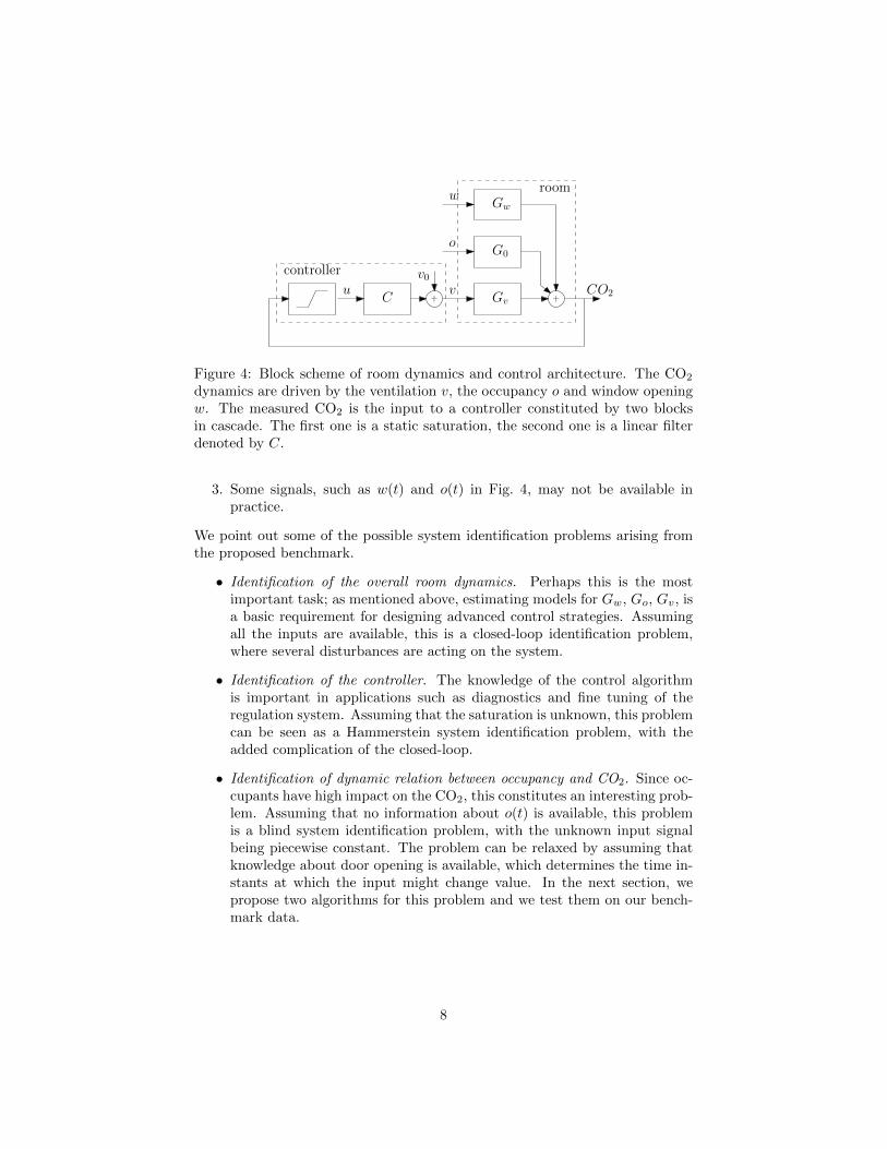
A schematic representation of the whole dynamics of interest is depicted inFig. 4. The signal CO2(t) can be thought of as the sum of three contributions.The first is given by possibly open windows, which are represented by the signalw(t) and influence the output through the system Gw. The second contributionis given by the occupancy, denoted by o(t), and the related dynamic systemGo. The third one is the result of the air ventilation acting on the room.The ventilation, denoted by v(t), is driven by a specific control system. Thecontroller can be seen as the cascade of a static nonlinearity, which acts asa saturation, and a linear controller, plus a constant source signal v0. Thesaturation receives the current value of the CO2 concentration and transformsit into the signal u according to the following map:

u(t) =

0 if CO2(t) < 700 ppm,CO2(t)−7001100−700 if 700 ppm ≤ CO2(t) ≤ 1100 ppm,

1 if CO2(t) > 1100 ppm.

(1)

6

Mon Tue

Op

en

ing

0

0.2

0.4

0.6

0.8

1

Window opening

Mon Tue

Occu

pa

ncy

0

2

4

6

8

10

Occupancy

Figure 3: Examples of window opening and occupancy conditions. Profiles forthe first two days of the simulated week are shown. Top: window opening signal.Bottom: number of occupants in the office.

Note that u(t) is not available to the experimenter. This signal is filtered by alinear filter (denoted by C in Fig. 4), which is a PID controller with unknownparameters. The resulting signal is then summed to a constant value v0, whichprovides a constant base ventilation to the room.

4.1 Related system identification problems

The dynamics described above give rise to several problems related to unmod-eled dynamics. Knowing the models Gw, Go, Gv and the controller architectureis a basic requirement to design intelligent regulation strategies. Quite unfor-tunately (or perhaps, from a system identification perspective, luckily), gettingthe aforementioned models seems to be a challenging task. This mainly becauseof three reasons:

1. Although the room dynamics could in principle be quite-well approxi-mated by linear systems, these systems could be time-varying, due toseasonal phenomena, etc.;

2. There is a number of non modelable phenomena (air leakages, computers,etc.) which might influence the room dynamics and should be regardedas noise;

7

Gv

G0

+C

o

CO2v

room

+

v0u

controller

Gww

Figure 4: Block scheme of room dynamics and control architecture. The CO2

dynamics are driven by the ventilation v, the occupancy o and window openingw. The measured CO2 is the input to a controller constituted by two blocksin cascade. The first one is a static saturation, the second one is a linear filterdenoted by C.

3. Some signals, such as w(t) and o(t) in Fig. 4, may not be available inpractice.

We point out some of the possible system identification problems arising fromthe proposed benchmark.

• Identification of the overall room dynamics. Perhaps this is the mostimportant task; as mentioned above, estimating models for Gw, Go, Gv, isa basic requirement for designing advanced control strategies. Assumingall the inputs are available, this is a closed-loop identification problem,where several disturbances are acting on the system.

• Identification of the controller. The knowledge of the control algorithmis important in applications such as diagnostics and fine tuning of theregulation system. Assuming that the saturation is unknown, this problemcan be seen as a Hammerstein system identification problem, with theadded complication of the closed-loop.

• Identification of dynamic relation between occupancy and CO2. Since oc-cupants have high impact on the CO2, this constitutes an interesting prob-lem. Assuming that no information about o(t) is available, this problemis a blind system identification problem, with the unknown input signalbeing piecewise constant. The problem can be relaxed by assuming thatknowledge about door opening is available, which determines the time in-stants at which the input might change value. In the next section, wepropose two algorithms for this problem and we test them on our bench-mark data.

8

5 The blind system identification challenge

In this section, we address the problem of identifying the dynamic relation be-tween occupancy and CO2. We assume we do not have access to the occupancysignal o, which is piecewise constant, but, having installed a sensor on the doorof the room, we know when this signal may change value.

With reference to Fig. 4, the dynamics of CO2 as function of o can bedescribed by the following closed-loop transfer function

Q =Go

1− CGv, (2)

where we have neglected the presence of the saturation. We consider a lineartime-invariant model for Q. Furthermore, we define the new output CO2(t) :=CO2(t)−CO2,0, where CO2,0 is the outdoor CO2 concentration (see Table 3 inAppendix) and model general uncertainties as white noise. Then we can rewritethe model in time domain

CO2(t) =

n∑k=1

q(k)o(t− k) + e(t) , (3)

where we have approximated the system dynamics with a (long) FIR of ordern. The term e(t) is the prediction error that contains the measurement noiseand is modeled as Gaussian white noise. We collect N samples of the output.Introducing a vector notation, we rewrite (3) as a linear regression problem,i.e. CO2 = Oq + e, where O is a suitable Toeplitz matrix containing o. Ifwe denote the door opening events by T1, T2 . . . Tp = N and define the matrixH = diag{1T1

,1T2−T1. . .1Tp−Tp−1

}, then we can write o = Hx, where x ∈ Rp

denotes the unknown occupancy levels. Using this notation, we now give twoalgorithms for this problem.

5.1 Benchmarking algorithms

5.1.1 Baseline method

This method is a re-adaptation of the Hammerstein system identification methodproposed in [3]. It consists of the following steps.

1. Define Φ =[H SH S2H . . . Sp−1H

], where S acts as one-position

downwards shifting matrix, so that we can rewrite CO2 = Φθ + e, whereθ := vec(qxT ).

2. Compute a least-squares estimate of θ and denote it by θ.

3. Form the n× p matrix Θ by reshaping θ.

4. Compute q as the first left singular vector of Θ and x as the first rightsingular vector of Θ.

A nice property of this method is that it can be proven to be asymptoticallyconsistent [3].

9

5.1.2 Kernel-based method

We test a recently proposed blind system identification method tailored for thistype of problem. It is based on kernel-based methods combined with the so-called stable spline kernel [17]. Due to space constraints, we do not providedetails on this method here, referring the interested reader to [4].

5.2 Testing the benchmarking algorithms on data

We evaluate the performance of the blind system identification algorithms de-scribed in the previous section on the data sets. Specifically, we run the iden-tification algorithms using daily data records and discarding data before 9:00and after 18:00. Also, we do not consider data regarding Saturday and Sunday,since the room is known to be empty. So, for each data set, we obtain 5 separateidentification problems, one for each weekday. We define two accuracy scores.

1. The fit of the CO2 signal, i.e.

FITCO2= 1−

√√√√ ∑270t=1 (CO2(t)− CO2(t))

2∑270t=1 (CO2(t)−mean[CO2(t)])

2 , (4)

where CO2(t) is the output predicted by the identified model and 270 isthe number of samples per interval considered.

2. The fit of the occupancy signal, namely

FITO = 1−

√√√√∑270t=1 (O(t)−O(t))

2∑270t=1O(t)

2 . (5)

Note that the average value of the true occupancy is not removed in thedenominator.

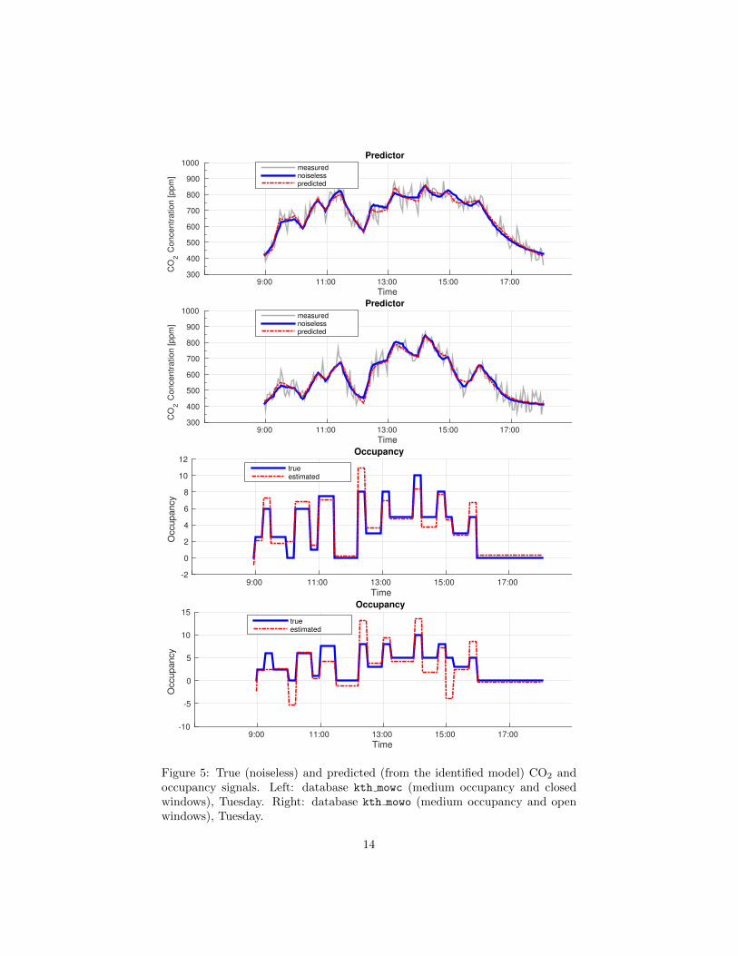
The overparameterization method is not able to capture the CO2 dynamicsnor reconstruct the occupancy pattern, always giving negative fits. Thus wedo not report its results. The identification performance of the kernel-basedmethod is summarized in Table 2, where the average (over the days) daily fitsare reported. Two examples of the resulting outcomes are shown in Fig. 5,where we see the CO2 profile predicted by the identified model, compared withthe noiseless CO2 profile in the dataset. When windows are kept closed, thereconstruction performance is satisfactory, giving fits ranging from 89.72 % to98.44 % in the CO2, and fits ranging from 72.86 % to 87.57 % in the occupancy.However, when open windows are simulated, the fits drop to 80.3 ÷ 87.24 % inthe CO2 and 37.85 ÷ 67.13 % in the occupancy. This indicates that the effect ofopen windows cannot be neglected when trying to perform blind identificationof the occupancy/CO2 relation.

10

Database Average occupancy fit (%) Average CO2 fit (%)

kth lowc 87.6 98.4kth mowc 76.2 92.8kth howc 72.9 89.7kth lowo 37.9 80.3kth mowo 39.4 87.2kth howo 67.1 86.0

Table 2: Average occupancy and prediction fits for the different databases.

6 Discussion

We have proposed and described a set of data generated from a simulated officeenvironment. The data set is targeted around those signals involved in the CO2

dynamics, such as ventilation inflow, window opening and number of people inthe room. Simulations were carried out using the commercial software IDA-ICEand were shown to well-describe a real laboratory at KTH. We have sketcheda schematic representation of the environment, pointing out some interestingproblems from the system identification perspective. Among these problems,we have attempted a blind identification of the dynamic relation between the(unknown) number of occupants and the CO2 signal.

We believe that the presented data can be potentially very interesting forthe system identification community, due to the numerous challenges arisingfrom this framework. This also holds true for researchers working in smartbuilding design, where the integration of smart devices with the building hasmade data-based modeling techniques of paramount importance.

This data set is continuously evolving: we plan to perform further sim-ulations taking into account other aspects of the office environment, such asexternal influences (solar radiation, outdoor temperature) and temperature dy-namics.

Appendix: Useful Parameters

References

[1] K. Abed-Meraim, W. Qiu, and Y. Hua. “Blind system identification”. In:Proc. IEEE 85.8 (1997), pp. 1310–1322.

[2] B. Ai, Z. Fan, and R. X. Gao. “Occupancy Estimation for Smart Build-ings by an Auto-Regressive Hidden Markov Model”. In: American ControlConference. 2014, pp. 2234–2239. isbn: 9781479932719.

[3] E. W. Bai. “An optimal two-stage identification algorithm for Hammerstein–Wiener nonlinear systems”. In: Automatica 34.3 (1998), pp. 333–338.

11

Parameter Value

Room height [m] 2.9Floor area [m2] 80Door area [m2] 1.6Total window area [m2] 2.56Number of windows [-] 4Minimum mechanical ventilation flow [m3/s] 0.08Maximum mechanical ventilation flow [m3/s] 0.28Building air tightness [ACH @ 50 Pa] 1.5Occupant activity level [MET] 1.8Maximum tuna fish weight [kg] 684Outdoor air CO2 concentration [ppm] 420Sampling time of the data [min] 3

Table 3: Some parameters of interest for the room dynamics.

[4] G. Bottegal, R. S. Risuleo, and H. Hjalmarsson. “Blind system identifica-tion using kernel-based methods”. In: Proc. IFAC Symp. System Identifi-cation (SYSID). Vol. 48. 28. 2015, pp. 466–471.

[5] A. Costa et al. “Building operation and energy performance: Monitoring,analysis and optimisation toolkit”. In: Applied Energy 101 (2013), pp. 310–316.

[6] D. B. Crawley et al. “Contrasting the capabilities of building energyperformance simulation programs”. In: Building and environment 43.4(2008), pp. 661–673.

[7] A. Ebadat et al. “Estimation of building occupancy levels through en-vironmental signals deconvolution”. In: Proc. ACM Workshop EmbeddedSystems For Energy-Efficient Buildings (BuildSys). Association for Com-puting Machinery (ACM), 2013.

[8] EQUA. EQUA Simulations AB: IDA-ICE website. June 2015. url: http://www.equa.se/en/ida-ice.

[9] P. Ferreira et al. “Neural networks based predictive control for thermalcomfort and energy savings in public buildings”. In: Energy and Buildings55 (2012), pp. 238–251.

[10] P. Fritzson. Principles of object-oriented modeling and simulation withModelica 2.1. John Wiley & Sons, 2010.

[11] Z. Han, R. X. Gao, and Z. Fan. “Occupancy and indoor environment qual-ity sensing for smart buildings”. In: Instrumentation and MeasurementTechnology Conference. May 2012, pp. 882–887. isbn: 978-1-4577-1772-7.

[12] IFAC. The IFAC TC 1.1 database Repository. June 2015. url: http:

//tc.ifac-control.org/1/1/Data\%20Repository.

12

[13] KTH-EES. The EES Smart Building website. June 2015. url: http://hvac.ee.kth.se.

[14] C. Liao, Y. Lin, and P. Barooah. “Agent-based and graphical modellingof building occupancy”. In: Journal of Building Performance Simulation5.1 (Jan. 2012), pp. 5–25. issn: 1940-1493.

[15] F. Oldewurtel et al. “Use of model predictive control and weather forecastsfor energy efficient building climate control”. In: Energy and Buildings 45(2012), pp. 15–27.

[16] A. Parisio et al. “Implementation of a Scenario-based MPC for HVACSystems: an Experimental Case Study”. In: Preprints of the 19th WorldCongress, The International Federation of Automatic Control. Vol. 10.2014, p. 10.

[17] G. Pillonetto et al. “Kernel methods in system identification, machinelearning and function estimation: A survey”. In: Automatica 50.3 (2014),pp. 657–682.

[18] P. Sahlin et al. “Whole-building simulation with symbolic DAE equationsand general purpose solvers”. In: Building and Environment 39.8 (2004),pp. 949–958.

[19] J. Siroky et al. “Experimental analysis of model predictive control for anenergy efficient building heating system”. In: Applied Energy 88.9 (2011),pp. 3079–3087.

[20] Z. Vana et al. “Model-based energy efficient control applied to an officebuilding”. In: Journal of Process Control 24.6 (2014), pp. 790–797.

13

Time9:00 11:00 13:00 15:00 17:00

CO

2 C

oncentr

ation [ppm

]

300

400

500

600

700

800

900

1000Predictor

measurednoiselesspredicted

Time9:00 11:00 13:00 15:00 17:00

CO

2 C

oncentr

ation [ppm

]

300

400

500

600

700

800

900

1000Predictor

measurednoiselesspredicted

Time9:00 11:00 13:00 15:00 17:00

Occu

pa

ncy

-2

0

2

4

6

8

10

12Occupancy

trueestimated

Time9:00 11:00 13:00 15:00 17:00

Occup

ancy

-10

-5

0

5

10

15Occupancy

trueestimated

Figure 5: True (noiseless) and predicted (from the identified model) CO2 andoccupancy signals. Left: database kth mowc (medium occupancy and closedwindows), Tuesday. Right: database kth mowo (medium occupancy and openwindows), Tuesday.

14