GYRO Simulations of Electron Transport: Particle Pinches & Finite beta

R. E. Waltz, J. Candy,G.M.Staebler, and F.L. HintonGeneral Atomics

C. Estrada-MilaUniversity of California at San Diego

J. E. KinseyLehigh University

ITPA Lisbon, Portugal Nov. 8-11,2004

Outline

GYRO Progress

Quick review of Bohm scaled DIIID L-mode pair

First steps to a steady state core gyrokinetic transport code

Preliminary work on gyroBohm scaled DIIID H-mode pair

Mechanisms breaking gyroBohm scaling: local versus non-local

Heuristic theory for non-local transport

Corrugated flux surface “equilibrium” profiles and local dynamos

Neoclassical flows embedded in turbulence

ExB shear quenching of electron driven turbulence

Plasma and impurity flow pinches

Beta scan benchmarks

Outline

Advanced GLF23 Transport Model

Better linear mode accuracy at high-a, low/high-s, steep gradients in pedestal

Real geometry

Nonlocal transport breaking gyroBohm

Hopefully a “linear mode calculation” of ExB shear quenching

GYRO is the most physically comprehensive global nonlinear gyrokinetic code

•GYRO is an Eulerian (continuum) [not PIC (Lagrangian) ] 5D gyrokinetic code. Development began in 1999 and design milestones completed in early 2003.

•GYRO operates both as a cyclic flux tube code (flat profiles at vanishing * ) or near full radius slice 0 boundary condition global code (profile variation with finite * ).

•GYRO is very versatile with all the physics needed for physically realistic simulations of all transport channels in a tokamak core plasma:

•toroidal ITG mode physics

•real tokamak geometry

•trapped and passing electrons

•finite beta

•e-i pitch angle collisions

•equilibrium sheared ExB and toroidal rotation profiles

•inputs real experimental profiles

== “full physics”

Some limitations and fundamentals about GYRO, global gyrokinetic codes, and broken gyroBohm scaling at finite *

•Standard gyrokinetic & Poisson-Ampere equations assume leading order in small * only.

Typically and < O(1%) [ see Frieman & Chen 1982; Antonsen & Lane 1980]

•GYRO consistently retains only this leading order in * : Thus in GYRO,

all finite * effect breaking gyroBohm scaling result from profile variation alone.

•GYRO will likely be inaccurate in a steep gradient pedestal where > O(10%). Consistently relaxing these small * approximations likely require 6D Vlasov equations.

•For flat profiles and all * , global GYRO with 0 BC gives the same gyroBohm scaled transport as the flux-tube GYRO with cyclic BC, i.e. the boundary conditions are “benign”.

•With profile variation, going from small to very small * , the local diffusivity from a global code approaches the the gyroBohm scaled diffusivity from a local flux tube code.

€

*

€

˜ n /n0

€

˜ n /n0

New GYRO features

• Facility for simulations at fixed flows rather than fixed gradients

• Neoclassical driver and Krook conserving ion-ion collisions

• Multispecies for impurity and plasma flow studies.

Realistic simulation of Bohm scaled DIII-D L-mode * pairTransport at slice center nearly independent of slice size suggests non-local effects are small and not responsible for Bohm scaling here.

€

χeff = (χ i + χ e ) /2

€

χGB = (cs /a)ρ s2

€

* ≡ ρ s /a

€

s ≡ cs /Ωi

• Bohm scaling is

€

χ / χ GB ∝1/ρ*

€

*(1.05T ) /ρ*(2.10T ) = 0.0040 /0.0026 ≈ 8 /5

• “Full physics” except =20 not 60 which is difficult for large slices sizes here.

• Transport 4x experimental levels for 20 but 2x experimental for physical = 60.

€

mi /me

€

mi /me

Movie

Get within 2x of experimental diffusivity with Bohm scaling only if retaining “Full Physics” (and real electron mass).

€

mi /me = 20⇒ 60

€

χeff / χ GB

€

ratio :8 /5⇒ 3.6 /2.2 = 1.64

• Turning off ExB, or e-i collisions, or betadrops from Bohm ratio 1.64 toward gyroBohm scaling ratio 1.00

All reduce

€

χeff / χ GB( flux tube no ExB) = 8

• Decreasing the ion temperature gradient by 5% gets to 1.5X exp.€

γnet =γmax −γE

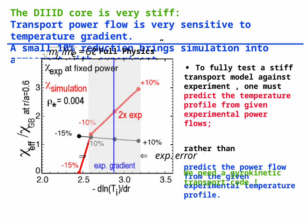
The DIIID core is very stiff:Transport power flow is very sensitive to temperature gradient.A small 10% reduction brings simulation into agreement with experiment

€

⇒

€

⇐ exp. error ?

€

mi /me = 60 “Full Physics”

• To fully test a stiff transport model against experiment , one must predict the temperature profile from given experimental power flows;

rather than

predict the power flow from the given experimental temperature profile.

We need a gyrokinetic transport code !

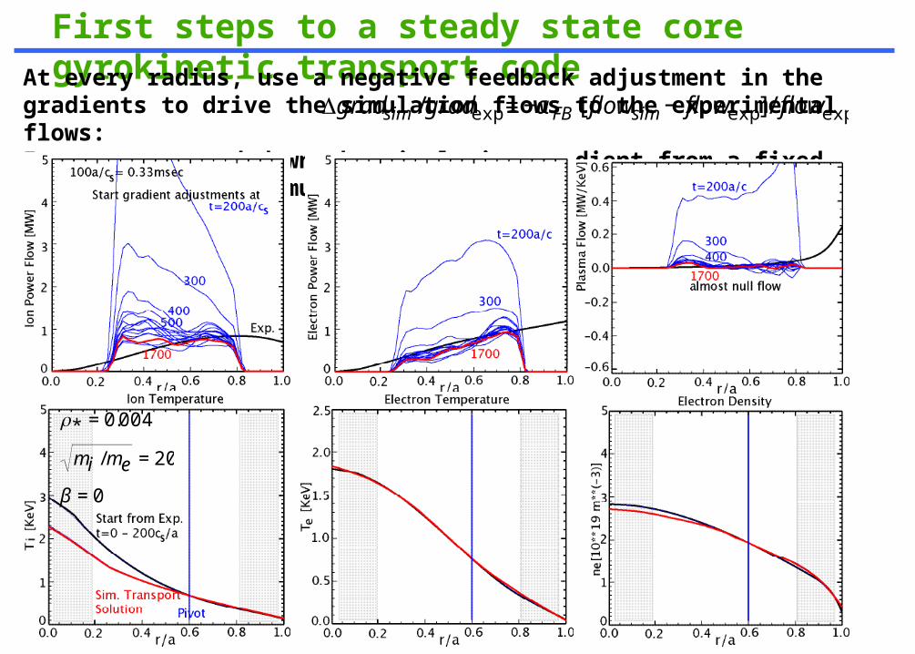
First steps to a steady state core gyrokinetic transport codeAt every radius, use a negative feedback adjustment in the gradients to drive the simulation flows to the experimental flows:Integrate up and down the simulation gradient from a fixed pivot to get the simulation profile.

€

Δgradsim /gradexp = −α FB[ flowsim − flowexp ]/ flowexp

€

* = 0.004

mi / me = 20

β = 0

• Because of core stiffness [a/LTi ] and near null plasma flow from a thermal pinch

[a/Ln vs a/LTe], adjustments to match experimental flows are small……..10-20% here.

€

* = 0.004

mi / me = 20

β = 0

• Within the next two years, we hope to have a gyrokinetic steady state core transport simulation with self-consistent fusion power for an ITER scale burning plasma given an H-mode pedestal boundary condition.

• This will operate as a master prototypical transport code driving many parallel slave gyrokinetic gyroBohm flux-tube simulations at each radius.

Preliminary gyroBohm DIIID H-mode simulations

• The similarity condition on the best DIIID H-mode are rather poor.

• The “gyroBohm” scaling actually tends to super-gyroBohm r/a < 0.7

• Nevertheless the GYRO simulation tracks the experiment

• Rescaling from data to we get exactly gyroBohm.

Local mechanisms breaking gyroBohm scaling The profile of maximum growth rate and ExB shear rate are exquisitely

matched, so Bohm scaling is not due to experimental dissimilarity.

Mode phase velocity shear rates can have a * dependence.

When there can be a significant stabilizing effect breaking gyroBohm scaling:

Contrast with empirical Mixed Bohm/gyroBohm Model:

This local shearing mechanism was previously discussed [Waltz et al IAEA 1996] and illustrated with ITG-ae simulations [Waltz, Candy & Rosenbluth APS 2001 and IAEA 2002]

However for the DIII-D L-mode * pair realistic “full physics” simulation

The * dependence of the velocity shearing rate seems too weak, to quantitatively account for the Bohm scaling.

€

γs =| γ* ± γ E |

€

γs /γ max ~ ρ* /ε ~ O(1)

€

χ ~ χ GB(1−γ s /γ max ) ~ χ GB(1− ρ* /ε)∝ χ GB(ε /ρ*)

€

χ ~ χ Bohmε '(1+ ρ* /ε)

€

γmax

€

γE

€

γs

Non-local mechanisms breaking gyroBohm scaling Linear toroidal coupling between singular surfaces gives a non-local mechanism which drains

turbulence from unstable regions and spreads turbulence into stable (or less unstable regions).

This non-local mechanism breaks gyroBohm scaling toward Bohm in the unstable regions:

and toward super-gyroBohm in the stable (or less unstable) regions:

This non-local mechanism was found to give a small breaking effect in ITG-ae simulation using realistic profiles with a central stable core but could account for transport in linearly stable central core plasmas or ITBs [Waltz, Candy & Rosenbluth APS 2001 and IAEA 2002]

Lin, Hahm et al [APS 2001 and IAEA 2002] using unphysical flat profiles with stable central core and edge, showed Bohm scaled ITG-ae simulations at * =0.008 (about 2x DIII-D values).

However the DIII-D L-mode * pair realistic “full physics” simulation had no stable edge and the stable core was not covered by the smaller simulation slices…yet Bohm persisted.

Thus it seems unlikely to us that this non-local mechanism gives a quantitative explanation. Nevertheless non-local effects can be important, and we have developed a heuristic model for

including them into gyroBohm local transport models like GLF23 [Waltz et al IAEA 1996]

€

χ ~ χ GB(1− ρ* /ε)

€

χ ~ χ GB(1+ ρ* /ε)

Simulations with non-local transport Simplified ITG-ae simulations with flat and piecewise flat profiles.

……. a/LT reduced 4-fold in left quarter of radial slice to get a stable region

• Lower driving rate increases the “non-local connection length” L ……….easier to get Bohm scaling nearer to threshold

• Adding an unphysical stable edge region to the right, doubles the drainage from the unstable region and makes Bohm scaling easier to get

Heuristic theory (model) for non-local transport

Local transport models (like GLF23) use quasilinear theory with the gyroBohm spectral weight

We propose to replace the local (net) growth rate by a non-local growth rate from radially averaging over the whole plasma (with a localized weight) :

BC: and

If then the global eigenmode growth rate. Both and are independent of * .

But for small * plasmas, global eigenmodes take a long time to form , and if the turbulence is more strongly driven, the zonal flows have larger ExB shearing rates and more quickly break up the global modes before they fully form.

Our heuristic theory argues which explains the piecewise flat profile simulations.

€

Ik (x) = [(e | ˜ φ k | /Te ) /ρ* ]2 ∝ γk _ locnet /[cs /a]

€

γknet (x) = dx ' /[2L(x' )]γk _ loc

net

−∞

∞∫ (x' )exp[− | x − x'| /L(x' )]

€

γk _ locnet

€

γk _ locnet (x'< 0) = γk _ loc

net (0)

€

γk _ locnet (x'> a) = γk _ loc

net (a)

€

γk (x)⇒ γk _ glob (x)

€

Tglob

€

˜ γ E

€

L /a∝1/[Tglob ˜ γ E ]∝ (ρ* / ˆ s )(a /R) /[γ locnet /(cs /a)]1/2

€

γk _ locnet

€

γk _ globnet

€

L /a ⇒ ∞

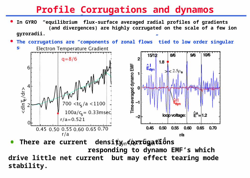
Profile Corrugations and dynamos In GYRO “equilibrium” flux-surface averaged radial profiles of gradients (and

divergences) are highly corrugated on the scale of a few ion gyroradii.

The corrugations are “components of zonal flows” tied to low order singular surfaces

€

∇ ˜ T ≈ ∇T0

• There are current density corrugations responding to dynamo EMF’s which drive little net current but may effect tearing mode stability.

• EMF(I) is from magnetic flutter (like the MHD - dynamo) and EMF(II) is electrostatic.€

jdyn / j0 = Edyn /E A

• “Equilibrium” here means 1-5 msec time average and (n=0) flux surface average.

• The corrugations are tied to singular surfaces and don’t wash out by “sloshing” around radially because singular surfaces do not move ……in GYRO…. i.e. q(r) is frozen !

Are these corrugations physically real ?

• “Equilibrium” here means 1-5 msec time average and (n=0) flux surface average.

• The corrugations are tied to singular surfaces and don’t wash out by “sloshing” around radially because singular surfaces do not move ……in GYRO…. i.e. q(r) is frozen !

• BUT should they move ? We should be able to compute (and self-consistently insert ?)

q(r) ----> q0(r) + q(r,t)

How big is r(r,t) ?

Are these corrugations physically real ?

“Cross-talk” between neoclassical and turbulent flows GYRO now has a conserving Krook ion-ion collisions and a neoclassical driver term to n=0 equation giving

the O(*) poloidal deviation to the equilibrium. Neoclassical flows result.

At * -->0 there is no “cross talk” between turbulent and neoclassical flows….they are additive.

For finite - * the cross talk appears to be small if any.

• The “turbulent” neoclassical flows are radial averages of the large orbit neoclassical flows (which deviate somewhat from the standard * -->0 flows .

• Plasma flow (not shown) is ambipolar (with conserving Krook and non-adiabatic part only)€

( ˜ f + ze ˜ φ /T )n=0υ Dx (θ )

EXB shear quenching and trapped electron driven modes The EXB shear quench rule: (s- geometry) has been extended from ITG to

trapped electron mode (TEM) turbulence: GA-Std case

For purely toroidal rotation, a large parallel shear rate can drive up faster than and no quench may result.

€

γE /γ max = 2 ± 0.5

€

γp = (Rq /r)γ E

€

γmax(γ p )

€

γE

€

Ln /LT

€

χi / χ GB

€

χe / χ GB

€

D / χ GB

ITG-ae 3/1 0.13, -0.31 3.54 ± 0.37

ITG/(TEM) 3/1 0.27, -0.33 10.7 ± 2.6 3.2 ± 0.6 -1.9 ± 0.5

ITG/TEM 2/2 0.28, -0.014 11.0 ± 2.2 11.3 ± 2.2 4.0 ± 0.8

TEM 2/3 0.43, +0.029 23.9 ± 3.7 27.7 ± 4.5 5.6 ± 0.9

€

[γ max ,ω]

€

a /LT = 3,a /Ln =1,R /a = 3,q = 2, s =1

€

γp = γ E = 0

Is there a “linear mode” calculation of EXB shear quenching?

• GLF23 uses quasilinear transport spectral weight

• where Can we calculate directly?

• No problem for “slab” geometry eigenmode, but toroidal geometry has Floquet mode oscillations of “instantaneous” growth rate with period .

• Can be identified with ?

€

Ik (x) = [(e | ˜ φ k | /Te ) /ρ* ]2 ∝ γknet /[cs /a]

€

γknet = γk

lin (γ p )−α Eγ E

€

E ≈ 0.4 − 0.7

€

γknet

€

2π ˆ s /γ E

€

γkinst (t)

€

γknet

€

γkinst

t

Plasma and impurity flow pinches Multi-species have been added to GYRO. Thermally pinched plasma flows and impurity pinches

are found to be in good agreement with the 1996 GLF23 model. Pure plasma thermal pinch driven by trapped electrons. Adding e-i collisions move null flow point to higher

The thermal pinch allows some peaking of null flow cores. Helium transport described by D-V paradigm:

GA Std. Case:

€

ηe = Ln /LTe

€

ΓHe = DHenHe /LHe = nHe[DdHe /LHe −VHe ]

€

a /LT = 3,a /Ln =1,R /a = 3,q = 2, s =1

Finite beta benchmarks CYCLONE base case:

€

a /LT = 2.48,a /Ln = 0.8,R /a = 2.78,r /a = 0.5,q =1.4, s = 0.78, mi /me = 42.

Note: growth rates decrease by about 50% to critical beta, then greatly increase (particularly for low k “ideal modes”.

Subdominant “kinetic ballooning mode” onsets just belowcritical beta.

Simulations very difficult approaching critical beta

Summary and Conclusions GYRO is the most physically comprehensive gyrokinetic code with the “full physics”

presently thought required to realistically simulate core tokamak transport in all channels.

Bohm scaled transport in DIII-D L-modes in matched *-pairs has been obtained.

ExB shear appears to be important in obtaining Bohm scaling in DIII-D L-mode.

GYRO simulations track the gyroBohm scaled DIII-D H-modes which have larger * but much lower ExB shear rates.

Core transport is stiff. Simulated core power and plasma flows can be matched with to experimental flows with small (10%) adjustments in the ion temperature gradients.

We demonstrated the first steps to a core gyrokinetic transport code. We have investigated both local velocity shear and non-local drainage mechanisms

for breaking gyroBohm scaling.

……But neither appear to give quantitatively accurate accounts of the Bohm scaling in the realistic DIII-D L-mode simulations.

Other recent conclusions (discussed in paper & poster) Simulations demonstrated a heuristic theory (model) for incorporating non-local transport in local

gyroBohm models (like GLF23) . The theory is based on linear toroidal coupling of singular surfaces and the partial formation of global modes broken up by zonal flows.

The model locally averages local growth rates over a length L

GYRO has shown that the equilibrium flux-surface averaged radial gradient (and divergence) profiles are highly corrugated on the scale of a few ion gyroradii and tied to singular surfaces.

“Dynamo” current density corrugations may affect tearing stability but do not produce much net current beyond the neoclassical current voltage relation

Ion-ion collisions and the neoclassical curvature drift drive was added to GYRO.

Even with large orbit effects (finite *), the “cross-talk” between turbulent and neoclassical flows appears to be weak.

The EXB shear quench rule: (s- geometry) has been extended from ITG to trapped electron mode (TEM) turbulence.

For purely toroidal rotation, a large parallel shear rate can drive up faster than and no quench may result.

Multi-species have been added to GYRO. Thermally pinched plasma flows and impurity pinches are found to be in good agreement with the 1996 GLF23 model.

€

γE /γ max = 2 ± 0.5

€

γp = (Rq /r)γ E

€

γmax(γ p )

€

γE

€

L /a∝1/[Tglob ˜ γ E ]∝ (ρ* / ˆ s )(a /R) /[γ locnet /(cs /a)]1/2

Progress to an Advanced GLF23 Transport Model 1996 GLF23 is simple and fast: Used 4 passing-i, 2 trapped-e & 2 passing-e GLF moments

X 1-theta wave function for low-k. High-k ETG used separate 4 passing-e X 1-(ballooning) theta wave function with adiabatic ions.

Gave a good fit to gyrokinetic ballooning mode linear stability rates near GA-Std. Case:

But does rather poorly in low & high-s and high- or high Ti/Te, particularly for large driving gradients characteristic of ITB’s or pedestals.

• To improve linear accuracy, a new more GLF elaborate closure with 12 passing and 3 trapped moments for each species (although 6 will suffice for ions if very low-k trapped ions are ignored) allows a single model to span low-k ITG/TEM continuously to high-k ETG. The GLF closure coefficients become functions of the trapped fraction. (M=21 or 30)

Further the theta wave functions are a set of N=1, 2 or more Hermite basis can improve accuracy as needed, allow for strong rotational shear distortions, and most importantly allow real geometry to be simply included .

The old 8x8 linear stability matrices are now much larger and more expensive (NM/8)3 , but we are presently looking for ways to speed the solutions and keep the new model practical.

Some quick example of improvements in linear stability:

€

a /LT = 3,a /Ln =1, R /a = 3,r /a =1/2,q = 2, s =1,α = 0,Ti /Te =1

Comparison of GLF With Kinetic Response

Using methodology of Beer et al. to determine the best closure coefficients, an excellent fit to the density response function is obtained

-0.50

0.0

0.50

1.0

-10 -5 0 5 10 15 20

Re - KineticRe - GLFIm - KineticIm - GLF

ω/ ωD

kIIv

th/ω

D=1

no ω*

-0.80

-0.40

0.0

0.40

0.80

-10 -5 0 5 10 15 20

Re - KineticRe - GLFIm - KineticIm - GLF

ω/ ωD

kIIv

th/ω

D=1

grad-n

-0.80

-0.40

0.0

0.40

0.80

-10 -5 0 5 10 15 20

Re - KineticRe - GLFIm - KineticIm - GLF

ω/ ωD

kIIv

th/ω

D=1

grad-T

Kinsey /Staebler

Slab trapped particle test ωk||vt)

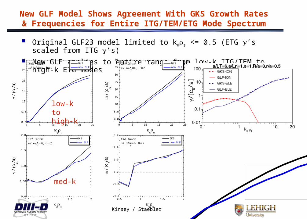
New GLF Model Shows Agreement With GKS Growth Rates & Frequencies for Entire ITG/TEM/ETG Mode Spectrum

Original GLF23 model limited to ks <= 0.5 (ETG γ’s scaled from ITG γ’s)

New GLF applies to entire range from low-k ITG/TEM to high-k ETG modes

0.0

5.0

10

15

20

25

30

0 5 10 15 20 25

GKS

new GLF

γ / (c

s/ )a

ky

s

Std Case/ /w a L

T=, =q

0.0

5.0

10

15

20

25

30

35

40

0 5 10 15 20 25

GKS

new GLF

ω / (c

s/ )a

ky

s

Std Case/ /w a L

T=, =q

0.0

0.50

1.0

1.5

2.0

0.5 1 1.5 2

GKS

new GLF

γ / (c

s/ )a

ky

s

Std Case/ /w a L

T=, =q

-2.0

-1.0

0.0

1.0

2.0

3.0

0.5 1 1.5 2

GKS

new GLF

ω / (c

s/ )a

ky

s

Std Case/ /w a L

T=, =q

low-kto high-k

med-k

Kinsey / Staebler

Kinsey - 9/04

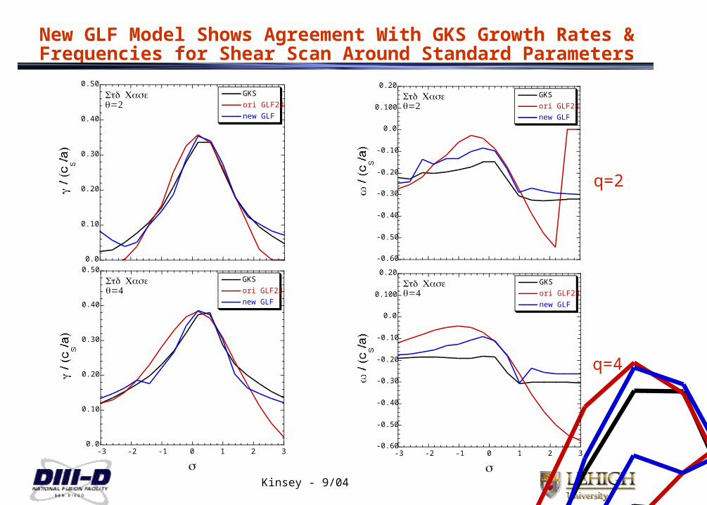
New GLF Model Shows Agreement With GKS Growth Rates & Frequencies for Shear Scan Around Standard Parameters

q=2

q=4

0.0

0.10

0.20

0.30

0.40

0.50GKS

ori GLF23

new GLF

γ / (c

s/ )a

St Cse

0.0

0.10

0.20

0.30

0.40

0.50

-3 -2 -1 0 1 2 3

GKS

ori GLF23

new GLF

γ / (c

s/ )a

s

Std Case=q

-0.60

-0.50

-0.40

-0.30

-0.20

-0.10

0.0

0.100

0.20GKS

ori GLF23

new GLF

ω / (c

s/ )a

Std Case=q

-0.60

-0.50

-0.40

-0.30

-0.20

-0.10

0.0

0.100

0.20

-3 -2 -1 0 1 2 3

GKS

ori GLF23

new GLF

ω / (c

s/ )a

s

Std Case=q

Kinsey - 9/04

New GLF Model Shows Improved Agreement For High Ti/Te

Similar agreement for ori GLF23, new GLF models with GKS for Ti/Te=1

Ti/Te=1

0.0

0.10

0.20

0.30

0.40

0.50GKS

ori GLF23

new GLF

γ / (c

s/ )a

St CseT

iT

e

-1.0

-0.80

-0.60

-0.40

-0.20

0.0GKS

ori GLF23

new GLF

ω / (c

s/ )a

Std CaseT

i/T

e=.

Ti/Te=2

0.0

0.10

0.20

0.30

0.40

0.50

0 0.1 0.2 0.3 0.4 0.5 0.6 0.7

GKS

ori GLF23

new GLF

γ / (c

s/ )a

ky

s

Std CaseT

i/T

e=.

-1.2

-0.80

-0.40

0.0

0.40

0.80

1.2

0 0.1 0.2 0.3 0.4 0.5 0.6 0.7

GKS

ori GLF23

new GLF

ω / (c

s/ )a

ky

s

St CseT

iT

e

Kinsey - 9/04

New GLF Model Significantly Better For NCS and Pedestal Parameters

Original GLF23 model does not describe growth rates and frequencies for large |s-|

New GLF model agrees with GKS for both NCS and pedestal cases with large shear and alpha

NCS case:STD+a/LTi=10, a/LTi=4,=3

0.0

0.20

0.40

0.60

0.80

1.0

-1 -0.5 0 0.5 1 1.5 2

GKS

ori GLF23

new GLF

γ / (c

s/ )a

s

NCS Case=q

0.0

0.50

1.0

1.5

1 2 3 4 5 6 7

GKS

ori GLF23

new GLF

s

PED Caseq=4

Pedestal case:STD+r/a=0.75, a/Ln=3, a/LTi,e=10, =9

Progress to an Advanced GLF23 Transport Model (cont’d) Option for gyroBohm breaking nonlocal transport will be added to the local model

This simply replaces local net growth rate in quasilinear spectrum with the nonlocal rate :

New transport code methods will be need to evaluate a stiff nonlocal transport Finally, we would like to find a way to build the ExB shear rate into a “some

kind of linear mode calculation” and bypass the “ExB quench rule”:

It has been hard to pin down the parametric dependence of and there is constant confusion for real geometry: Waltz vs. Hahm-Burrell definition of .

€

Ik (x) = [(e | ˜ φ k | /Te ) /ρ* ]2 ∝ γk _ locnet /[cs /a]

€

γk _ locnet (x)⇒ γk

net (x) = dx ' /[2L(x' )]γk _ locnet

−∞

∞∫ (x' )exp[− | x − x'| /L(x' )]

€

γk _ locnet (x'< 0) = γk _ loc

net (0)

€

γk _ locnet (x'> a) = γk _ loc

net (a)

€

γk _ locnet

€

L /a∝1/[Tglob ˜ γ E ]∝ (ρ* / ˆ s )(a /R) /[γ locnet /(cs /a)]1/2

€

Ik (x)

€

γknet

€

γE€

γk _ locnet ⇒ γk _ loc

mod e (γ E )

€

γk _ locnet = γk _ loc

balloon −α Eγ E

€

γE

€

E