The theory of Bernoulli Shiftsby Paul C. Shields

Professor Emeritus of MathematicsUniversity of Toledo, Toledo, OH 43606

Send corrections to bshifts@earthlink.net

Web Edition 1.01Reprint of 1973 University of Chicago Press edition

With some error correction

Made available to the mathematics communityby the author, with no copyright restrictions.

Thanks to Andrew Shields for typing assistance.

PREFACE to this Web Edition 1.01

The University of Chicago Press decided to take this book out of print andkindly returned the copyright to me. I arranged for my son, Andrew, to retypethe manuscript as a LATEX document. The result is uncopyrighted and is availableto those who wish to use it without permission. The format has been changed,including page numbering; some errors have been corrected; and there have beensome changes in wording in a few places. The theorem and lemma numbering haveremained the same. Figures were redone by me to fit into the LATEX framework.

Please send any corrections and comments to bshifts@earthlink.net.The first edition was dedicated to my mother and father, this edition is also.

03/10/03. Seattle, WA

PREFACE to 1973 edition.

There are many measure spaces isomorphic to the unit interval with Lebesguemeasure, hence there are many ways to describe measure-preserving transforma-tions on such spaces. For example, there are translations and automorphisms ofcompact metric groups, shifts on sequence spaces (such as those induced by sta-tionary processes), and flows arising from mechanical systems. It is a natural ques-tion to ask when two such transformations are isomorphic as measure-preservingtransformations. Such concepts as ergodicity and mixing and the study of uni-tary operators induced by such transformations have provided some rather coarseanswers to this isomorphism question.

The first major step forward on the isomorphism quesion was the introductionby Kolmogorov in 1958-59 of the concept of entropy as an invariant for measure-preserving transformation. In 1970, D. S. Ornstein introduced some new approx-imation concepts which enabled him to establish that entropy was a complete in-variant for a class of transformations known as Bernoulli shifts. Subsequent workby Ornstein and others has shown that a large class of transformations of physicaland mathematical interest are isomorphic to Bernoulli shifts.

These lecture notes grew out of my attempts to understand and use these newresults about Bernoulli shifts. Most of the material in these notes is concerned withthe proof that two Bernoulli shifts with the same entropy are isomorphic. Thisproof makes use of a number of simple ideas about partitions and approximationby periodic transformations. These are carefully presented in Chapters 2-6. Thebasic results about entropy are sketched in Chapters 7-8. Ornstein’s FundamentalLemma is proved in Chapter 9. This enables one to construct partitions withperfect distribution and entropy close to those which are almost perfect, and is thekey to obtaining the isomorphism theorem in Chapter 10. Chapters 11-13 containextensions of these results, while Chapter 1 contains a summary of the measuretheory used in these notes. For a more complete account of recent extensions ofthese ideas, the reader is referred to D. S. Ornstein’s forthcoming notes ([42]).

I am particularly grateful to D. S. Ornstein, who introduced me to most of theideas in this book. I also wish to thank R. L. Adler, N. A. Friedman, Y. Katznelson,R. McCabe, and B. Weiss for many helpful converstions, and R. Newman, whodrew most of the pictures. Thanks are also due to James England, Robert Field,Richard Lacey, Douglas Lind, Stephen Polit, and Michael Steele, who read theoriginal manuscript with great care, correcting numerous errors and giving manysuggestions for improvement. The manuscript was typed by Elizabeth Plowman.Special thanks are due her for her patience and care.

This work was supported in part by NSF grants GP 33581X and GJ 776.

1

CHAPTER 1.LEBESGUE SPACES

This chapter describes the properties of spaces isomorphic to the unit intervalthat will be used, frequently without reference, in the sequel.

Our measure spaces (X,Σ, µ) will always be assumed to be finite, completespaces; that is, µ(X) is finite and Σ contains all subsets of sets of measure zero. Ifµ(X) = 1, the space (X,Σ, µ) is called a probability space. All sets and functionsare assumed (or must be shown to be) Σ-measurable and our measure spaces areassumed to be probability spaces, unless stated otherwise. Equality is taken tomean ”equality mod zero”; for example, two sets A,B are equal if µ(A4 B) = 0where A4B is the symmetric difference (A−B) ∪ (B − A).

An isomorphism φ of (X1,Σ1, µ1) onto (X2,Σ2, µ2) is a mapping φ : X1 → X2

such thatφ(Σ1) ⊆ Σ2, φ−1(Σ2) ⊆ Σ1,

µ2(φ(A1)) = µ1(A1), A1 ∈ Σ1; µ1(φ−1(A2)) = µ2(A2), A2 ∈ Σ2,

and φ is one-to-one and onto (mod zero), that is, there are sets X i ⊆ X i such thatµi(X i − X i) = 0 , and φ is a one-to-one map of X1 onto X2 .

A space isomorphic to the unit interval with Lebesgue sets and Lebesgue mea-sure will be called a Lebesgue space. We sketch here Rohlin’s characterization ofsuch spaces (see [18]).

A collection E ⊆ Σ separates X if there is a set E ∈ Σ, µ(E) = 0, such that ifx, y 6∈ E, there is a set A ∈ E such that x ∈ A, y 6∈ A or x 6∈ A, y ∈ A. A collectionE generates Σ if Σ is the smallest complete σ-algebra containing E . A countablecollection E = {An} is complete in X if each intersection ∩∞n=1Bn is nonemptywhere, for each n, Bn is either An or Acn. If we let An be the set of all x in the unitinterval such that the nth digit in the binary expansion of x is 0, then it is easy tosee that {An} is a complete, separating, generating collection for the unit interval.The unit interval is also nonatomic; that is, any set of positive measure containssubsets of smaller positive measure. The space (X,Σ, µ) is a subspace of (X,Σ, µ)if X ∈ Σ, Σ consists of the sets A ∩ X, A ∈ Σ, and µ(A) = µ(A), A ∈ Σ. Wethen have the result

THEOREM 1.1. A probability space (X,Σ, µ) is a Lebesgue space if and onlyif it is a subspace of a probability space (X, Σ, µ) which has a complete, separating,generating sequence.

This theorem provides us with a large collection of Lebesgue spaces. For ex-ample, if X is a compact metric space, µ is a regular nonatomic Borel proba-blility measure, and Σ is the completion of the Borel sets with respect to µ, then(X,Σ, µ) is a Lebesgue space. Also, if (X,Σ, µ) is a Lebesgue space, and if X1 ∈ Σ,

2

µ(X1) > 0, then (X1,Σ1, µ1) is a Lebesgue space where Σ1 = {A∩X1|A ∈ Σ} andµ1(A) = µ(A)/µ(X1). One can also easily show that a countable direct product ofLebesgue spaces is a Lebesgue space.

We list here two important properties of Lebesgue spaces.

THEOREM 1.2. If (X,Σ, µ) is a Lebesgue space, then a collection E ⊆ Σseparates X if and only if it generates Σ.

THEOREM 1.3. Let (X i,Σi, µi) be Lebesgue spaces for i = 1, 2, and letφ : X1 → X2 be a measurable measure-preserving mapping; that is, φ−1(Σ2) ⊆Σ1 and µ1(φ−1(A2)) = µ2(A2), A2 ∈ Σ2. If φ is one-to-one (mod zero) then φ isonto (mod sero); in particular, φ(X1) must then be Σ2-measurable.

We will make use of Theorem 1.3 in conjunction with the following more elemen-tary result, which enables us to extend isomorphisms from generating collectionsto the entire σ-algebra.

THEOREM 1.4. Let σ:X1 7→ X2, where (X1,Σ1, µ1) and (X2,Σ2, µ2) areprobability spaces. Let E be a generator for Σ2, and suppose

(i) φ−1(E) ⊆ Σ1

(ii) µ1(φ−1(A)) = µ2(A), A ∈ E .Then φ−1(Σ2) ⊆ Σ1, and (ii) holds for all A ∈ Σ2.

This result is proved by first extending (i) and (ii) to the algebra generatedby E , then using the basic uniqueness theorem on extensions of measures (see [8],Theroem A, p. 54).

We now describe a factor space construction that will be useful in Chapter 10.Let (X,Σ, µ) be a probability space, and let Σ1 be a complete sub-σ-algebra of Σ.We say that x ∼ y if x and y cannot be separated by Σ1, and denote the set ofequivalence classes modulo this relation by X1. For x ∈ X, let π(x) denote theequivalence class of x. Define

Σ1 = {A ⊂ X1|π−1(A) ∈ Σ1}µ1(A) = µ(π−1(A)), A ∈ Σ1.

The space (X1,Σ1, µ1) is called the factor space of (X,Σ, µ) by Σ1. One can nowprove:

THEOREM 1.5. If (X,Σ, µ) is a Lebesgue space, and Σ1 is a complete nonatomicsub-σ-algebra, then the factor space (X1,Σ1, µ1) is a Lebesgue space.

Unless stated otherwise, all spaces in this book are assumed to be Lebesguespaces, and a transformation is an automorphism of such a space; that is, atransformation is an invertible measure-preserving mapping of a space isomorphicto the unit interval.

3

CHAPTER 2.SHIFTS AND PARTITIONS

We begin this chapter by giving a precise definition of a Bernoulli shift. Supposeπ = (p1, p2, . . . , pk), with pi > 0 and Σpi = 1. Let X be the set of all doublyinfinite sequences of the symbols 1, 2, . . . , k; that is, the set of all functions fromthe integers Z into {1, 2, . . . , k}. A measure is defined on X as follows: A cylinderset is a subset of X determined by a finite number of values, such as

C = {x|xi = ti,−m ≤ i ≤ n}(2.1)

where ti, −m ≤ i ≤ n, is some fixed finite sequence in {1, 2, . . . , k}. Let E denotethe σ-algebra generated by the cylinder sets. There is then a unique measure µdefined on E such that, if C has the form (2.1), then µ(C) =

∏ni=−m pti . The

measure space (X,Σ, µ) , where Σ is the completion of E with respect to µ, will becalled the product space with product measure µ determined by the distribution π.The transformation T defined by

(Tx)n = xn+1, n ∈ Z,

is clearly an invertible µ-measure-preserving transformation. It will be called theBernoulli shift with distribution π and denoted by Tπ.

There are many ways of determining the space (X,Σ, µ) ; that is, it has manyisomorphisms, so a given Bernoulli shift can be described in many other ways. Wegive here one simple geometric representation for the case when π = (1/2, 1/2).For convenience we shall use the indexing {0, 1}, rather than {1, 2}; that is, Xwill be the set of all doubly infinite sequences of zeros and ones. Given x ∈ X,construct the point (s(x), t(x)) in the unit square (using binary digits)

s(x) = .x0x1x2 . . .

t(x) = .x−1x−2x−3 . . .

The mapping x → (s(x), t(x)) is easily seen to be one-to-one and onto (afterremoving a set from X of µ-measure zero). Furthermore, this mapping carries theclass Σ onto the class of Lebesgue sets and µ into Lebesgue measure on the unitsquare. Also,

s(Tx) = .x1x2 . . .

t(Tx) = .x0x−1x−2 . . .

so that T is carried onto the Baker’s transformation (see Fig. 2.1).

4

Step 1. Cut unit square into twocolumns of equal width.

A Bx•

Step 2. Squeeze each column to a rectangle of height 1/2 and base 1.

A′x• B′

Step 3. Put A′ on top of B′ to forma square.

A′

B′

Tx•Fig 2.1

5

Obviously, this construction can be generalized. For example, if π = (1/3, 1/3, 1/3),then, using ternary expansions, the shift T with distribution π becomes the Baker’stransformation indicated in Figure 2.2.

Step 1. Cut unit square into threecolumns of equal width.

A B

x•

C

Step 2. Squeeze each column to a rectangle of height 1/3 and base 1

A′x• B′ C ′

Step 3. Put B′ on top of A′

and C ′ on top of B′

to form a square

A′

B′

Tx•

C ′

Fig 2.2

Are the transformations of Figures 2.1 and 2.2 isomorphic? That is, can we findan invertible measure-preserving transformation of the square (except for a null set)onto itself which carries one transformation into the other? More generally, if πand π are given distributions, when will Tπ be isomorphic to Tπ? The answer tothis general question is summarized in

THE KOLMOGOROV-ORNSTEIN ISOMORPHISM THEOREM. Two Bernoullishifts Tπ, Tπ are isomorphic if and only if

k∑i=1

pi log pi =k∑i=1

pi log pi(2.2)

where π = (p1, p2, . . . , pk), π = (p1, p2, . . . , pk).

6

The necessity of the condition (2.2) was established by Kolmogorov ([9], [10]),while Ornstein ([13]) established its sufficiency. In this monograph we describe indetail the ideas behind Ornstein’s results.

The concepts and terminology associated with partitions will enable us to givea more abstract and useful description of Bernoulli shifts. A partition P of X isan ordered finite disjoint collection of (measurable) sets (called the atoms of P )whose union is X. If P and Q are partitions, then P refines Q if each atom in Qis a union of atoms in P . If P refines Q, we write P ⊃ Q or Q ⊂ P . If P and Qare partitions, their join is

P ∨Q = {Pi ∩Qj|Pi ∈ P , Qj ∈ Q}

with lexicographic ordering. Clearly, P∨Q is the least partition which refines bothP and Q. For sequences of partitions P i, −m ≤ i ≤ n, we use the notation

n∨i=−m

P i = P−m ∨ P−m+1 ∨ . . . ∨ Pn.

A partition P determines a σ-algebra Σ(P), which is just the set of all unions ofmembers of P . Note that

P ⊃ Q iff Σ(P) ⊃ Σ(Q),

and that Σ(P ∨Q) is the smallest σ-algebra containing Σ(P) and Σ(Q).The distribution of a partition P = {P1, P2, . . . , Pk} is the vector

d(P) = (µ(P1), µ(P2), . . . , µ(Pk)).

If T is a transformation and P is a partition, then TP = {TPi|Pi ∈ P} and,for example,

n∨0

T iP = P ∨ TP ∨ . . . ∨ T nP .

We say that P is a generator for T if Σ is the smallest complete σ-algebra containing⋃∞n=−∞ T

nP .For example, consider the 2-shift T = Tπ with π = (1/2, 1/2) and the partition

P = {P0, P1}, where

P0 = {x|x0 = 0}, P1 = {x|x0 = 1}.

In this case, d(P) = (1/2, 1/2), and the sets in∨n−m T

iP are exactly the cylindersets {x|x−i = ti,−m ≤ i ≤ n} as (t−m, t−m+1, . . . , tn) ranges over all possiblesequences of zeros and ones, m + n + 1 units long. The tranformation T is the

7

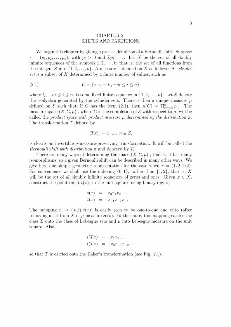
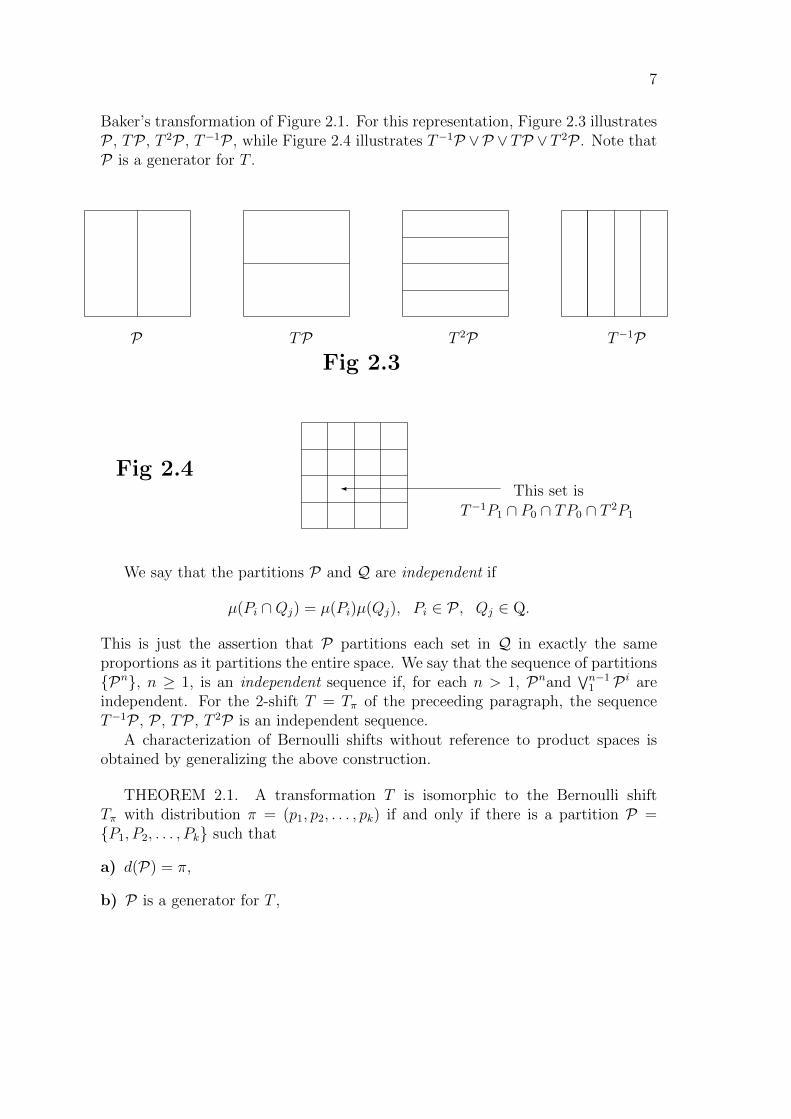
Baker’s transformation of Figure 2.1. For this representation, Figure 2.3 illustratesP , TP , T 2P , T−1P , while Figure 2.4 illustrates T−1P ∨P ∨ TP ∨ T 2P . Note thatP is a generator for T .

P TP T 2P T−1PFig 2.3

� This set isT−1P1 ∩ P0 ∩ TP0 ∩ T 2P1

Fig 2.4

We say that the partitions P and Q are independent if

µ(Pi ∩Qj) = µ(Pi)µ(Qj), Pi ∈ P , Qj ∈ Q.

This is just the assertion that P partitions each set in Q in exactly the sameproportions as it partitions the entire space. We say that the sequence of partitions{Pn}, n ≥ 1, is an independent sequence if, for each n > 1, Pnand

∨n−11 P i are

independent. For the 2-shift T = Tπ of the preceeding paragraph, the sequenceT−1P , P , TP , T 2P is an independent sequence.

A characterization of Bernoulli shifts without reference to product spaces isobtained by generalizing the above construction.

THEOREM 2.1. A transformation T is isomorphic to the Bernoulli shiftTπ with distribution π = (p1, p2, . . . , pk) if and only if there is a partition P ={P1, P2, . . . , Pk} such that

a) d(P) = π,

b) P is a generator for T ,

8

c) T nP , n ≥ 1, is an independent sequence.

Proof. Let T = T π be the Bernoulli shift with distribution π, and let Xπ

be the product space with product measure µπ determined by π. Put P ={P1, P2, . . . , Pk}, where

Pi = {x|x0 = i}.

Clearly, P is a generator for T (since the cylinder sets are just the atoms of∨n−m T

iP) and {T nP} is an independent sequence (since the product measure isused). This proves the existence of a P satisfying (a), (b), (c) for the Bernoullishift Tπ.

The proof of the converse makes use of the ideas sketched in Chapter 1. AssumeT and P satisfy (a), (b), (c), where T is defined on (X,Σ, µ) . We obtain a map φfrom X into Xπ as follows: If x ∈ X, then φ(x) = {xn} ∈ {1, 2, . . . , k}Z , where

xn = i iff T nx ∈ Pi.

It is obvious that φ(Tx) = T π(φ(x)). We wish to show that φ is an isomorphism;that is, except for a set of measure zero in X and a set of measure zero in Xπ, φis one-to-one, onto, measurable and measure-preserving.

The assumption that P is a generator for T means that the countable collectionof sets

⋃∞−∞ T

iP generates Σ; hence it also separates X (see Theorem 1.2). Thusthere is a set E ⊂ X of measure zero such that φ is one-to-one on X − E.

The proof that φ is measurable and measure-preserving is obtained by exam-ining the action of φ−1 on cylinder sets. Let

A =n⋂

i=−mT iPti , A = {x ∈ Xπ|xi = ti,−m ≤ i ≤ n}.

Then φ−1(A) = A (in the sense that µ(φ−1(A)4A) = 0). Also, since the indepen-dence condition (c) gives

µ(A) =n∏

i=−mµ(T iPti) =

n∏i=−m

µπ({x ∈ Xπ|xi = ti}),(2.3)

we see that µ(φ−1(A)) = µπ(A). It follows that φ is measurable and measure-preserving (Theorem 1.4), and hence maps onto a measurable set of measure onein X (Theorem 1.3). This proves Theorem 2.1.

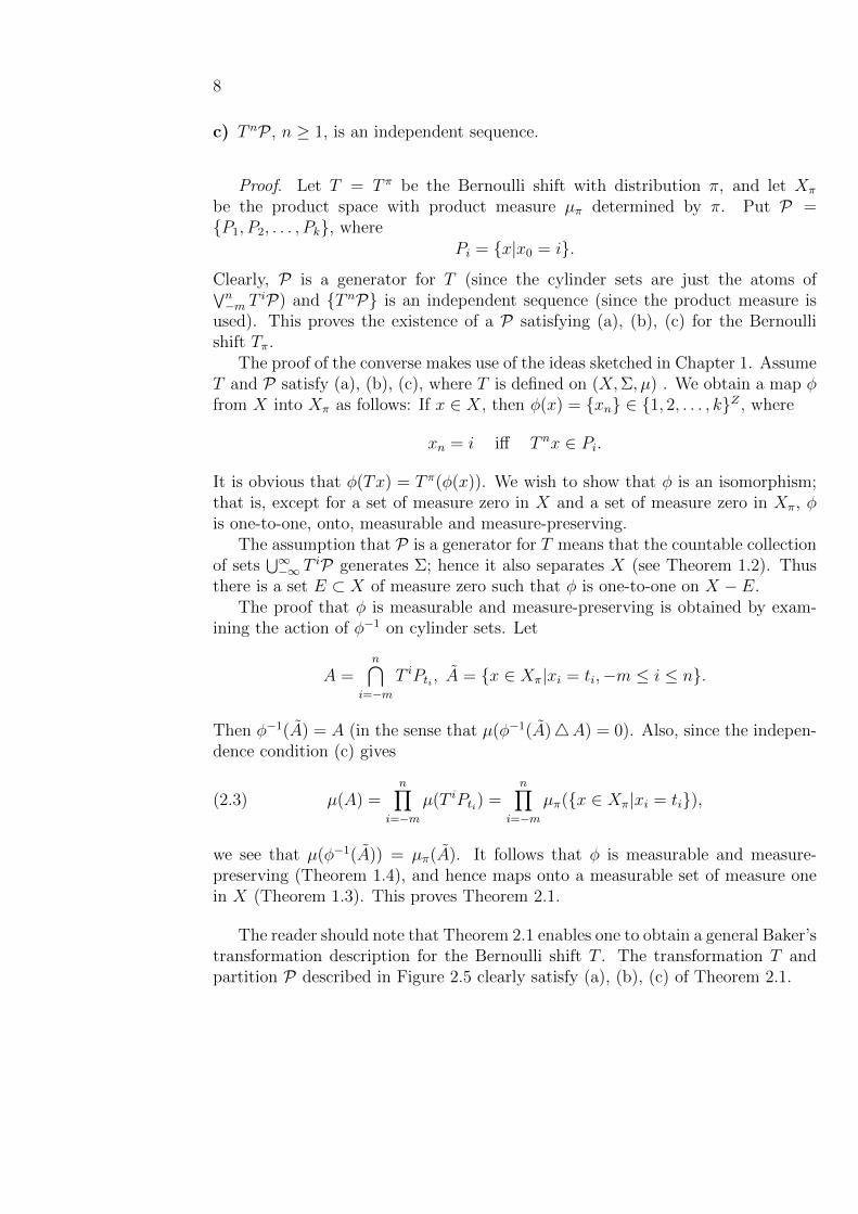
The reader should note that Theorem 2.1 enables one to obtain a general Baker’stransformation description for the Bernoulli shift T . The transformation T andpartition P described in Figure 2.5 clearly satisfy (a), (b), (c) of Theorem 2.1.

9

···

···P1 P2

(a)

P3

(a) Cut square into columnsP1, . . . , Pk with µ(Pi) = pi

(b) Squeeze each Pi to rectangleof width 1 and height pi

P ′1 P ′2 P ′3 . . .(b)

. . .

TP1

TP2

TP3(c) (c) Put P ′2 on top of P ′1, P ′3 on top

of P2,′ . . ., to form a square.

Fig. 2.5

The proof of Theorem 2.1 includes a useful concept. Suppose P = (P1, P2, . . . , Pk)is a partition and T is a transformation. The P-name of a point x is the bilateralsequence {xn} ⊆ {1, 2, . . . , k}, where

xn = i if x ∈ T−nPi; that is, T nx ∈ Pi.

Theorem 2.1 is just the observation that, if P is an independent generator for T ,then the map

x→ P-name of X

is an isomorphism which carries T into Tπ, the Bernoulli shift with distributionπ = d(P). This result is a special case of the fact that a stochastic process isdetermined by its joint distributions ([2]). In our case, the process is defined by

Zn(x) = i if x ∈ T−nPi;(2.4)

that is, the P-name of x is the sequence {Zn(x)}. This process is stationary, andits joint distributions are given by (2.3). To say that {T nP} is an independent

10

sequence is just the same as saying that {Zn} is a sequence of independent, iden-tically distributed random variables. These remarks can easily be generalized toyield the following result:

THEOREM 2.2. The transformations T and T are isomorphic if and only ifthere are partitions P and P which are generators for T and T , respectively, suchthat

d(n∨0

T iP) = d(n∨0

TiP), n = 0, 1, 2, . . . .

We close this section by stating a version of the law of large numbers, whichwill be needed in the sequel. Suppose P is a partition and A is a set in

∨n−10 T−iP ,

so that A has the form

A = Pi0 ∩ T−1Pi1 ∩ . . . ∩ T−n+1Pin−1 .

The sequence (i0, i1, . . . , in−1) will be called the P -n-name of A. Note that, in fact,A consists of all points x such that

xm = im, 0 ≤ m ≤ n− 1,

where {xm} is the P -name of X. Let fA(i, n) be the relative frequency of occurrenceof i in the P -n-name of A, that is,

fA(i, n) =|{t : xt = i, 1 ≤ t ≤ n}|

n.

We then have

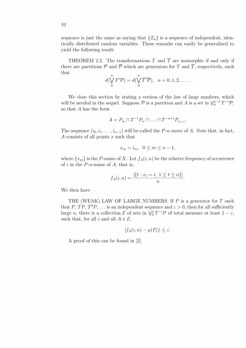
THE (WEAK) LAW OF LARGE NUMBERS. If P is a generator for T suchthat P , TP , T 2P , . . . is an independent sequence and ε > 0, then for all sufficientlylarge n, there is a collection E of sets in

∨n0 T−iP of total measure at least 1 − ε,

such that, for all i and all A ∈ E ,

|fA(i, n)− µ(Pi)| ≤ ε.

A proof of this can be found in [2].

11

CHAPTER 3.STACKS

The key to an understanding of Ornstein’s proof of the isomorphism theoremand to a number of other results is a simple geometric representation of a transfor-mation. The representation is valid for transformations which are aperiodic (thatis, for each n, µ{x : T nx = x} = 0), but we shall use it only for ergodic transfor-mations. A transformation is ergodic if TA ⊆ A implies µ(A) = 0 or µ(A) = 1.

The simplest way to prove that a Bernoulli shift is ergodic is to establish themuch stronger condition

limnµ(T nA ∩B) = µ(A)µ(B), A,B ∈ Σ.(3.1)

A transformation satisfying (3.1) is said to be mixing. A mixing transformationis obviously ergodic (merely apply (3.1) with B = Ac). To verify that a Bernoullishift is mixing, one first verifies that (3.1) holds for cylinder sets (where it is justthe statement that two cylinder sets that depend upon different coordinates areindependent). It follows that (3.1) holds for all sets by approximating with cylindersets.

The following theorem, due to Rohlin (see [7], p. 71), provides us with ourdesired representation.

ROHLIN’S THEOREM. If T is ergodic, n is a positive integer, and ε is apositive number, then there is a set F such that F , TF , T 2F , . . . , T n−1F is adisjoint sequence, and µ(

⋃n−1i=0 T

iF ) ≥ 1− ε.

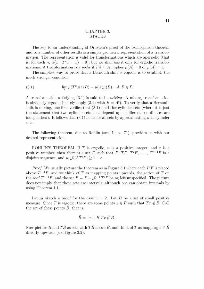
Proof. We usually picture the theorem as in Figure 3.1 where each T iF is placedabove T i−1F , and we think of T as mapping points upwards, the action of T onthe roof T n−1F , and the set E = X−⋃n−1

0 T iF being left unspecified. The picturedoes not imply that these sets are intervals, although one can obtain intervals byusing Theorem 1.1.

Let us sketch a proof for the case n = 2. Let B be a set of small positivemeasure. Since T is ergodic, there are some points x ∈ B such that Tx 6∈ B. Callthe set of these points B; that is,

B = {x ∈ B|Tx 6∈ B}.

Now picture B and TB as sets with TB above B, and think of T as mapping x ∈ Bdirectly upwards (see Figure 3.2).

12

F

TF

T 2F

T n−1F

6

6

x

Tx

T 2x

.

.

.Figure 3.1

� -B

6

B

TB = B1

x

Tx

.

.Figure 3.2

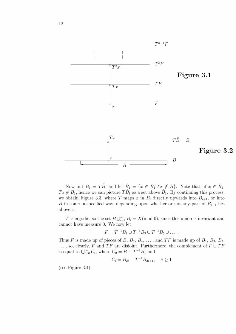
Now put B1 = TB, and let B1 = {x ∈ B1|Tx 6∈ B}. Note that, if x ∈ B1,Tx 6∈ B1, hence we can picture TB1 as a set above B1. By continuing this process,we obtain Figure 3.3, where T maps x in Bi directly upwards into Bi+1, or intoB in some unspecified way, depending upon whether or not any part of Bi+1 liesabove x.

T is ergodic, so the set B⋃∞i=1Bi = X(mod 0), since this union is invariant and

cannot have measure 0. We now let

F = T−1B1 ∪ T−1B3 ∪ T−1B5 ∪ . . . .Thus F is made up of pieces of B, B2, B4, . . . , and TF is made up of B1, B3, B5,. . . , so, clearly, F and TF are disjoint. Furthermore, the complement of F ∪ TFis equal to

⋃∞i=0 Ci, where C0 = B − T−1B1 and

Ci = B2i − T−1B2i+1, i ≥ 1

(see Figure 3.4).

13

6

6

6

B

B1

B2

B3

B4

x

Tx

.

.

x

T 2x

T 3x

6T 4x.

�

?

-

.

.

T 4x returns to B since B4 doest not lie above T 3x

Figure 3.3

B

B1

B2

B3

B4

B5

B6

B7

C0 = D0 D1

C1

D2

C2

D3

C3

********************************

**********************

**************

******

F

TF ******

Ci = the part of B2i that does not lie below B2i+1

Figure 3.4

14

It follows that

µ(∞⋃i=0

Ci) =∞∑i=0

µ(Ci) =∞∑i=0

µ(Di),

where Di = T−2iCi (again see Figure 3.4). Since the Di are disjoint and containedin B, we have

µ(F ∪ TF ) ≥ 1− µ(B),

so that, if µ(B) ≤ ε, F has the desired properties.Thus Rohlin’s theorem is just the observation that one can obtain a picture like

Figure 3.3, then regroup parts of the sets to obtain a picture like Figure 3.1.

Let us introduce some terminology associated with these results. The disjointsequence T iF , 0 ≤ i ≤ n− 1, will be called a stack of height n. In a slight abuse ofterminology, we shall use the symbol T for the restriction of T to

⋃n−2i=0 T

iF . Thisrestricted T is a map from

⋃n−2i=0 T

iF onto⋃n−1i=1 T

iF such that T : T iF → T i+1F .In order to describe the basic connections between P -names and stacks, we

extend some of our previous terminology. If P is a partition and A is a set ofpositive measure, then the partition induced on A by P is

P/A = {P1 ∩ A,P2 ∩ A, . . . , Pk ∩ A},

and the induced distribution is the vector

d(P/A) = (µA(P1), µA(P2), . . . , µA(Pk)),

where µA is the conditional measure defined by µA(B) = µ(B∩A)/µ(A). The P -n-name of a point x is the sequence (i0, i1, . . . , in−1) where Tmx ∈ Pim , 0 ≤ m ≤ n−1.Thus

∨n−10 T−iP/A is the partition of A into sets of points with the same P -n-name.

To see the relation between this and stacks, suppose T iF , 0 ≤ i ≤ n− 1, is a stackof height n. P induces a partition P/T iF on each level T iF of the stack (see Figure3.5).

F

F

T 2F

T 3F

TF

******* *************

************ ***********

******************

******* *****************

Superimpose above on copy of F below

A B C D E G B

C = P2 ∩ T−1P1 ∩ T−2P2 ∩ T−3P1 ∩ F

P1

P2

*******

The atoms of ∨30T−iP/F are the sets A,B,C,D,E,G,B

Figure 3.5

15

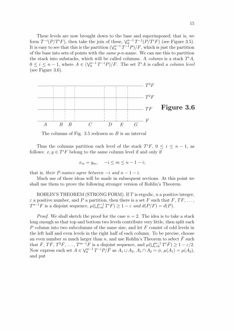
These levels are now brought down to the base and superimposed; that is, weform T−i(P/T iF ), then take the join of these,

∨n−10 T−1(P/T iF ) (see Figure 3.5).

It is easy to see that this is the partition (∨n−1

0 T−1P )/F , which is just the partitionof the base into sets of points with the same p-n-name. We can use this to partitionthe stack into substacks, which will be called columns. A column is a stack T iA,0 ≤ i ≤ n − 1, where A ∈ (

∨n−10 T−1P )/F . The set T iA is called a column level

(see Figure 3.6).

F

T 2F

T 3F

TF

A B B C D E G

The columns of Fig. 3.5 redrawn so B is an interval

Figure 3.6

Thus the columns partition each level of the stack T iF , 0 ≤ i ≤ n − 1, asfollows: x, y ∈ T iF belong to the same column level if and only if

xm = ym, −i ≤ m ≤ n− 1− i;

that is, their P -names agree between −i and n− 1− i.Much use of these ideas will be made in subsequent sections. At this point we

shall use them to prove the following stronger version of Rohlin’s Theorem.

ROHLIN’S THEOREM (STRONG FORM). If T is ergodic, n a positive integer,ε a positive number, and P a partition, then there is a set F such that F , TF , . . . ,T n−1F is a disjoint sequence, µ(

⋃n−1i=0 T

iF ) ≥ 1− ε and d(P/F ) = d(P ).

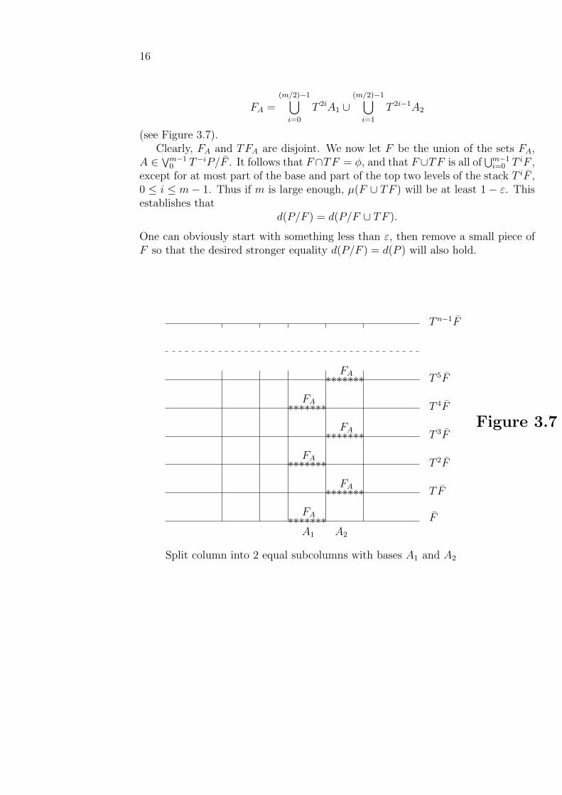
Proof. We shall sketch the proof for the case n = 2. The idea is to take a stacklong enough so that top and bottom two levels contribute very little, then split eachP column into two subcolumns of the same size, and let F consist of odd levels inthe left half and even levels in the right half of each column. To be precise, choosean even number m much larger than n, and use Rohlin’s Theorem to select F suchthat F , T F , T 2F , . . . , Tm−1F is a disjoint sequence, and µ(

⋃m−1i=0 T iF ) ≥ 1− ε/2.

Now express each set A ∈ ∨m−10 T−iP/F as A1 ∪A2, A1 ∩A2 = φ, µ(A1) = µ(A2),

and put

16

FA =(m/2)−1⋃i=0

T 2iA1 ∪(m/2)−1⋃i=1

T 2i−1A2

(see Figure 3.7).Clearly, FA and TFA are disjoint. We now let F be the union of the sets FA,

A ∈ ∨m−10 T−iP/F . It follows that F∩TF = φ, and that F∪TF is all of

⋃m−1i=0 T iF ,

except for at most part of the base and part of the top two levels of the stack T iF ,0 ≤ i ≤ m− 1. Thus if m is large enough, µ(F ∪ TF ) will be at least 1− ε. Thisestablishes that

d(P/F ) = d(P/F ∪ TF ).

One can obviously start with something less than ε, then remove a small piece ofF so that the desired stronger equality d(P/F ) = d(P ) will also hold.

F

T 2F

T 3F

T F

T 4F

T 5F

T n−1F

*******

*******

*******

FA

FA

FA

FA

FA

FA

*******

*******

*******

A1 A2

Split column into 2 equal subcolumns with bases A1 and A2

Figure 3.7

17

CHAPTER 4.GADGETS

We now wish to look more carefully at the column structure induced on ann-stack by a partition P . Labels can be assigned to column levels according to theset in P to which the level belongs. This gives a one-to-one map from columns intoP -n-names. It is then shown that any one-to-one map into n-strings of symbolsfrom any alphabet gives rise to a partition Q, which induces the same columnsas P . We also show how one can construct isomorphic copies of a given columnstructure.

To facilitate this discussion, we introduce the terminology used in [13]. A gadgetis a quadruple (T, F, n, P ), where T is a transformation, F a set such that F , TF ,T 2F , . . . , T n−1F is a disjoint sequence, and P a partition of

⋃n−1i=0 T

iF . As wasnoted in the previous chapter, P partitions each level P/T iF . If these are broughtdown to F and superimposed, one obtains

n−1∨0

T−i(P/T iF ) =n−1∨

0

T−iP/F.

The latter is the partition of the base into sets of points with the same P -n-names.The column CA with base A ∈ ∨n−1

0 T−iP/F is the stack T iA, 0 ≤ i ≤ n − 1.The points x, y ∈ T iF belong to the same column level iff xm = ym, −i ≤ m ≤(n− 1)− i.

We shall now assign the P -n-name of a column to that column and use this tolabel the column levels. To be precise, suppose P = {P1, P2, . . . , Pk}. The P -nameof a column CA in the gadget (T, F, n, P ) is the P -n-name of A; that is, the P -nameof CA is (i0, i1, . . . , in−1) if and only if the A has the following form.

A = F ∩ Pi0 ∩ T−1Pi1 ∩ . . . ∩ T−n+1Pin−1 .(4.1)

The mapping from columns into P -names of columns is a one-to-one map ofcolumns into sequences of {1, 2, . . . , k} of length n. Each column level is nowassigned one of the integers in {1, 2, . . . , k} according to the corresponding term inits column name; that is, if the P -name of CA is (i0, i1, . . . , in−1), then the label ofTmA is im. This means (from 4.1) that A ⊆ T−mPim (see Figure 4.1).

18

F

T 2F

T 3F

TF

A B C D E G

1 0 2 1 1 1

12 2 1 2 2

1 1 2 2 2 1

1 2 1 2 2 2

The labeling of Figure 3.6

Figure 4.1

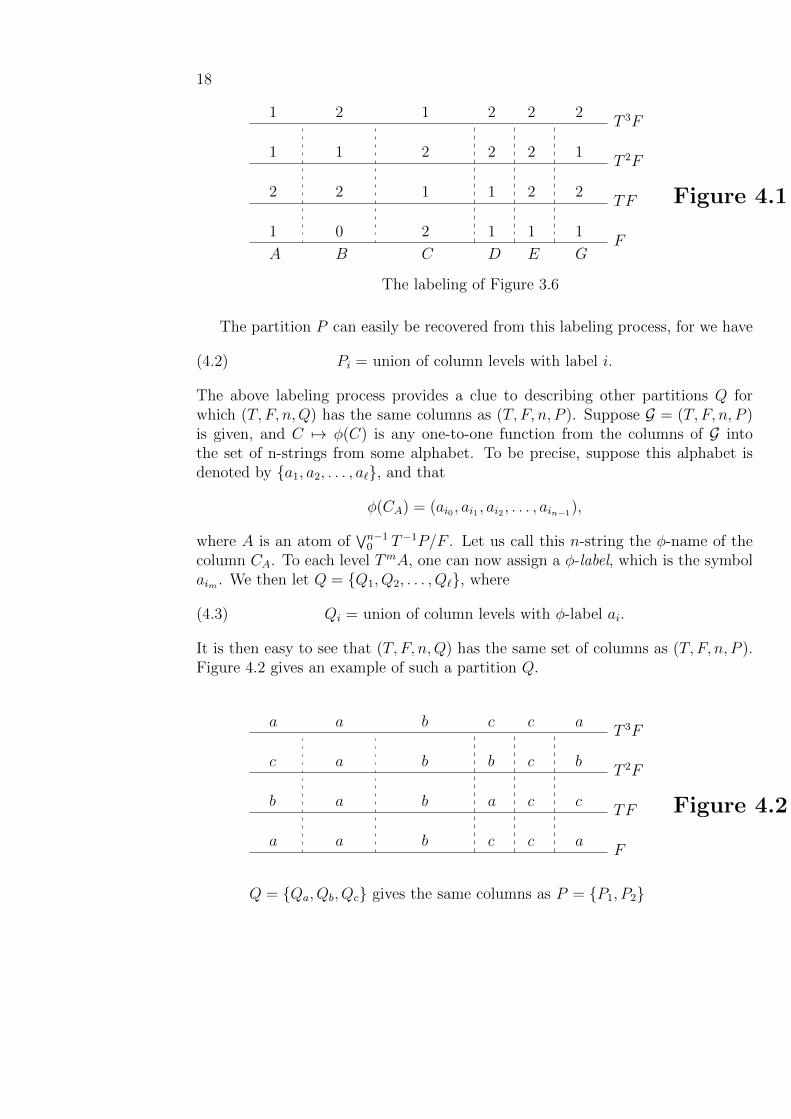
The partition P can easily be recovered from this labeling process, for we have

Pi = union of column levels with label i.(4.2)

The above labeling process provides a clue to describing other partitions Q forwhich (T, F, n,Q) has the same columns as (T, F, n, P ). Suppose G = (T, F, n, P )is given, and C 7→ φ(C) is any one-to-one function from the columns of G intothe set of n-strings from some alphabet. To be precise, suppose this alphabet isdenoted by {a1, a2, . . . , a`}, and that

φ(CA) = (ai0 , ai1 , ai2 , . . . , ain−1),

where A is an atom of∨n−1

0 T−1P/F . Let us call this n-string the φ-name of thecolumn CA. To each level TmA, one can now assign a φ-label, which is the symbolaim . We then let Q = {Q1, Q2, . . . , Q`}, where

Qi = union of column levels with φ-label ai.(4.3)

It is then easy to see that (T, F, n,Q) has the same set of columns as (T, F, n, P ).Figure 4.2 gives an example of such a partition Q.

F

T 2F

T 3F

TF

a a b c c a

bb a a c c

c a b b c b

a a b c c a

Q = {Qa, Qb, Qc} gives the same columns as P = {P1, P2}

Figure 4.2

19

For ease of reference, we summarize this result and its converse in the followinglemma.

LEMMA 4.1. Let G = (T, F, n, P ) be a given gadget, and let φ be a givenone-to-one function from columns of G into n-strings from some finite alphabet. IfQ is the partition formed by (4.3), then (T, F, n,Q) has the same set of columnsas (T, F, n, P ). Conversely, if Q = {Q1, Q2, . . . , Q`} is any partition such that(T, F, n,Q) has the same set of columns as (T, F, n, P ), then the mapping

C 7→ Q-name of C

is a one-to-one mapping from the columns into the set of Q-n-names.

The following lemma gives a further connection between the partition P andthe partition Q, when (T, F, n, P ) and (T, F, n,Q) have the same set of columns.

LEMMA 4.2. Suppose (T, F, n, P ) and (T, F, n,Q) have the same set of columns.Let H denote the two-set partition {F, F c} of the set G =

⋃n−1i=0 T

iF . Then

P/G ⊂n−1∨−n+1

T i(Q ∨H)/G.

Proof. The lemma is a consequence of the following simple fact.

If B and B are distinct column levels with B ⊆ T iF , B ⊆T jF , then either i 6= j or i = j, and, for some m, −i ≤ m ≤n−1− i, the two sets TmB and TmB have different Q-labels.

(4.4)

To complete the proof, let E be the partition into column levels

E = {CA ∩ T iF |A ∈n−1∨

0

T−jP/F, 0 ≤ i ≤ n− 1}.

The ordering of E is not important. We can then rephrase (4.4) as the statement

E ⊂n−1∨−n+1

T i(Q ∨H).

Since P/G is refined by E , the lemma follows.

Now we turn to the question of isomorphism of gadgets. We shall say that(T, F, n, P ) is isomorphic to (T , F , n, P ) if

d(n−1∨

0

T−1P/F ) = d(n−1∨

0

T−1P /F );

20

that is, P -n-names partition F in the same proportions as corresponding P -n-names partition F . It is implicit in this definition that the two gadgets have thesame height, and that P and P have the same number of sets. It is easy to seethat (T, F, n, P ) is isomorphic to (T , F , n, P ) if and only if there is an invertiblemapping S : F 7→ F such that, for all measurable A ⊂ F and A ⊂ F , we have

µ(A)/µ(F ) = µ(SA)/µ(F ),

µ(S−1A)/µ(F ) = µ(A)/µ(F ),

and, for x ∈ F , the P -n-name of x and the P -n-name of Sx are the same. Inother words, except for a possible change of scale, two gadgets are isomorphic ifone cannot distinguish between them by examining their column structures.

The statement that two gadgets are isomorphic says very little about their re-spective transformations, for Rohlin’s Theorem and a simple construction combineto give the following result.

LEMMA 4.3. If (T, F, n, P ) is any gadget and T is any ergodic transformation,then, for any ε > 0, there is a set F and a partition P such that (T , F , n, P ) is agadget isomorphic to (T, F, n, P ) and µ(

⋃n−1i=0 T

iF ) ≥ 1− ε.Proof. The proof makes use of the fact that, given any partition P of X and any

nonatomic space Y , one can partition Y in the same proportions as P partitionsX; that is, there is a partition Q of Y such that d(P ) = d(Q). With this in mind,use Rohlin’s Theorem to find F such that F , ¯TF , . . . , T n−1F is a disjoint sequenceand µ(

⋃n−1i=0 T

iF ) ≥ 1− ε. Then let Q be a partition of F such that

d(Q) = d(n−1∨

0

T−1P/F ).(4.5)

A Q-column will then be a stack T iA, A ∈ Q. The correspondence between P -n-names and sets of Q given implicitly by (4.5) then gives a one-to-one map φof Q-columns into P -n-names. Just as before, this means that each Q-column isassigned a P -n-name, which means that each Q-level is assigned a P -label. Thisgives a partition P of

⋃n−1i=0 T

iF into sets with the same label (as in (4.3)). Clearly,(T, F, n, P ) will then be isomorphic to (T , F , n, P ).

We will make use of an extension of Lemma 4.3, which is easily established bysimilar arguments:

LEMMA 4.4. Suppose (T, F, n, P ) is isomorphic to (T , F , n, P ), and Q isa partition of

⋃n−10 T iF . Then there is a partition Q of

⋃n−10 T iF such that

(T, F, n, P ∨Q) is isomorphic to (T , F , n, P ∨ Q).

Of course, Lemmas 4.3 and 4.4 tell us nothing about the action of T and T onthe top and complement of their gadgets, where almost anything can happen. Weshall later see how entropy can be used to control the relationsip between T andT .

21

CHAPTER 5.METRICS ON PARTITIONS

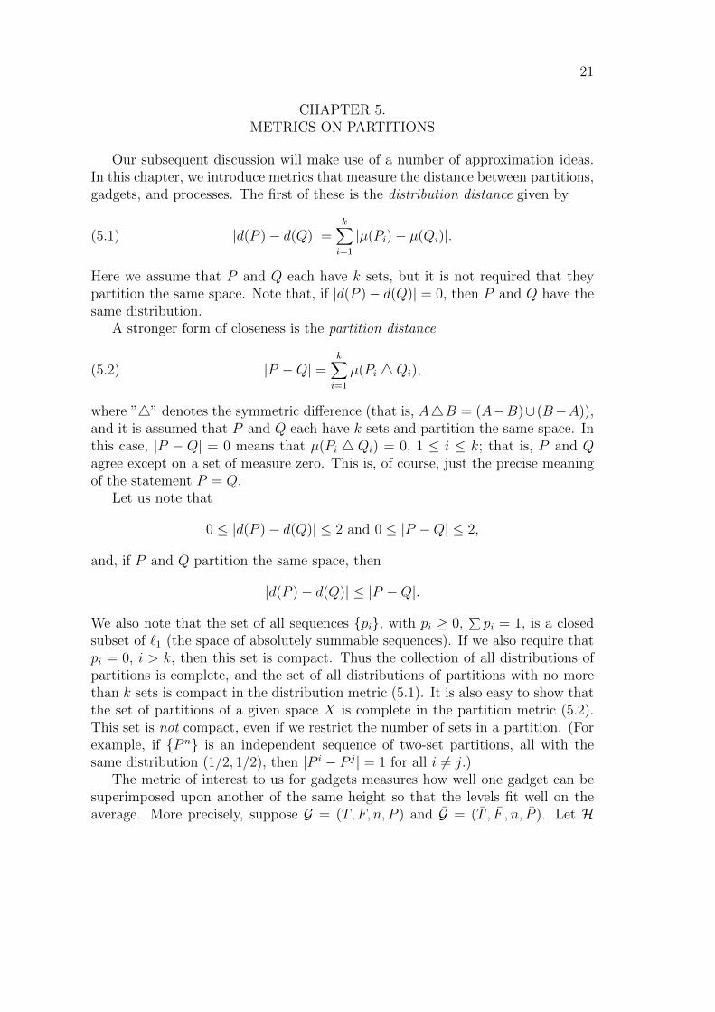
Our subsequent discussion will make use of a number of approximation ideas.In this chapter, we introduce metrics that measure the distance between partitions,gadgets, and processes. The first of these is the distribution distance given by

|d(P )− d(Q)| =k∑i=1

|µ(Pi)− µ(Qi)|.(5.1)

Here we assume that P and Q each have k sets, but it is not required that theypartition the same space. Note that, if |d(P )− d(Q)| = 0, then P and Q have thesame distribution.

A stronger form of closeness is the partition distance

|P −Q| =k∑i=1

µ(Pi4Qi),(5.2)

where ”4” denotes the symmetric difference (that is, A4B = (A−B)∪ (B−A)),and it is assumed that P and Q each have k sets and partition the same space. Inthis case, |P − Q| = 0 means that µ(Pi 4 Qi) = 0, 1 ≤ i ≤ k; that is, P and Qagree except on a set of measure zero. This is, of course, just the precise meaningof the statement P = Q.

Let us note that

0 ≤ |d(P )− d(Q)| ≤ 2 and 0 ≤ |P −Q| ≤ 2,

and, if P and Q partition the same space, then

|d(P )− d(Q)| ≤ |P −Q|.

We also note that the set of all sequences {pi}, with pi ≥ 0,∑pi = 1, is a closed

subset of `1 (the space of absolutely summable sequences). If we also require thatpi = 0, i > k, then this set is compact. Thus the collection of all distributions ofpartitions is complete, and the set of all distributions of partitions with no morethan k sets is compact in the distribution metric (5.1). It is also easy to show thatthe set of partitions of a given space X is complete in the partition metric (5.2).This set is not compact, even if we restrict the number of sets in a partition. (Forexample, if {P n} is an independent sequence of two-set partitions, all with thesame distribution (1/2, 1/2), then |P i − P j| = 1 for all i 6= j.)

The metric of interest to us for gadgets measures how well one gadget can besuperimposed upon another of the same height so that the levels fit well on theaverage. More precisely, suppose G = (T, F, n, P ) and G = (T , F , n, P ). Let H

22

be the set of all partitions Q of⋃n−1i=0 T

iF such that (T, F, n,Q) is isomorphic to(T , F , n, P ). In other words, if Q ∈ H, then (T, F, n,Q) is a copy of G on the stackT iF , 0 ≤ i ≤ n− 1. The gadget distance is then

dn(G, G) = infQ∈H

1

n

n−1∑i=0

|P/T iF −Q/T iF |.(5.3)

Since a gadget isomorphism can be implemented by a transformation, this defini-tion can also be formulated as follows: Let E be the set of all invertible mappingsS : F 7→ F , such that

µ(A)/µ(F ) = µ(SA)/µ(F ), A ⊂ F ,

µ(S−1A)/µ(F ) = µ(A)/µ(F ), A ⊂ F.

Extend S to a mapping of⋃n−1i=0 T

iF onto⋃n−1i=0 T

iF by defining ST ix = T iSx,x ∈ F . Then

(5.3a) dn(G, G) = infS∈E

1

n

n−1∑i=0

|P/T iF − SP/T iF |.

It is quite easy to show that dn(G, G) = 0 if and only if G and G are isomorphic.We also note that

dn(G, G) ≤ |d(n−1∨

0

T−iP/F )− d(n−1∨

0

T−1P /F )|,

so that, if the P -n-names and the P -n-names of points in the respective basesare close in distribution, the gadgets are close. The converse of this is not true.There is, however, a sense in which the P -n-names and P -n-names are close. Thissurprising and useful result is a consequence of the following lemma.

LEMMA 5.1. Suppose (T, F, n, P ) and (T, F, n,Q) are gadgets satisfying

1

n

n−1∑i=0

|P/T iF −Q/T iF | < ε2.(5.4)

Let E be the set of points x ∈ F such that the P -n-name and the Q-n-name of xdiffer in more than εn places. Then µ(E) ≤ εµ(F ).

Proof. Let Ej be the set of points x ∈ F such that the P -n-name and Q-n-nameof X differ in the jth place; that is,

Ej = T−jk⋃i=1

[(Pi ∩ T jF )4 (Qi ∩ T jF )].

23

The condition (5.4) then gives

n−1∑j=0

µ(Ej) ≤ nε2µ(F ),

while the definition of E tells us that

εnXE ≤n−1∑j=0

XEj,

where XA denotes the characteristic function of A. Now integrate to obtain

εnµ(E) ≤n−1∑j=0

µ(Ej) ≤ nε2µ(F ),

which gives the desired conclusion. This proves Lemma 5.1.

If the names of most points agree in most places, then the levels must be closeon the average. This converse to Lemma 5.1 is stated as

LEMMA 5.2. Let E be the set of points x ∈ F such that the P -n-name andQ-n-name of x differ in more than εn places, and suppose µ(E) ≤ εµ(F ). Then

1

n

n−1∑i=0

|P/T iF −Q/T iF | ≤ 3ε.(5.5)

In particular, |P/G−Q/G| = 1/n∑n−1i=0 |P/T iF −Q/T iF |, so

|P/G−Q/G| ≤ 3ε,(5.6)

where G =⋃n−1i=0 T

iF .

Proof. This is proved by using the column structure of the gadget. Let E bethe class of sets of the form

C = A ∩B ∩ Ec,

A ∈n−1∨

0

T−iP/F, B ∈n−1∨

0

T−iQ/F.

The column T jC, 0 ≤ j ≤ n − 1, is then the intersection of the two columns{T j(A ∩ Ec)} and {T j(B ∩ Ec)}.

Since C ∩E = φ, all except at most εn of the levels T jC have identical P - andQ-labels. In particular, we have

1

n

n−1∑j=0

|P/T jC −Q/T jC| ≤ 2ε.(5.7)

24

For each j, we have

|P/T jF −Q/T jF | = =∑i

µ(T−j(Pi4Qi) ∩ F )

µ(F )

=∑C∈E|P/T jC −Q/T jC| · µ(C)

µ(F )

+∑i

µ(T−j(Pi4Qi) ∩ E)

µ(F ).

The hypothesis that µ(E) ≤ εµ(F ) and the result (5.7) then yield the desired result(5.5). This proves Lemma 5.2.

A number of our later results will be most easily stated in terms of an extensionof this gadget metric to processes. Let T and T be transformations defined X,X, respectively, and with respective partitions P and P . The process distance isdefined by

d((T, P ), (T , P )) = supn

infS∈E

1

n+ 1

n∑i=0

|T iP − ST iP |,(5.8)

where E is the class of all isomorphisms of X onto X. The full significance of thismetric is still somewhat unclear (see some of the discussion in Chapter 10 belowand [16]). It will primarily be used in this paper to simplify the statements of anumber of results.

We mention here some of the properties of the process metric (5.8). First, wenote that the supremum used in (5.8) is actually a limit. This follows from the factthat, if infS∈E 1/n

∑n−1i=0 |T iP−ST iP | = α, then, for all r, infS∈E 1/nr

∑nr−1i=0 |T iP−

ST iP | ≥ α. We also observe that

If P and P are generators for T and T , and and ifd((T, P ), (T , P )) = 0, then T is isomorphic to T .

(5.9)

The proof of (5.9) is as follows: The condition that d((T, P ), (T , P )) = 0 impliesthat, for each n,

infS∈E

1

n

n−1∑i=0

|T iP − ST iP | = 0,

and hence that d(∨n−1

0 T iP ) = d(∨n−1

0 T iP ), n = 1, 2, . . . . Theorem 2.2 thenimplies that (5.9) is true.

The following lemma is established in much the same way as Lemmas 5.1 and5.2.

LEMMA 5.3. If d((T, P ), (T , P )) < ε2, then, for each n, there is an isomorphismSn from X to X such that the set of points x ∈ X for which the P -n-name of x

25

and the P -n-name of S−1n x differ in more than εn places has measure less than ε.

Conversely, the existence of such an Sn implies that d((T, P ), (T , P )) < 3ε.

An equivalent form of the definition (5.8) can be obtained by superimposingT, P and T , P on a third space. In fact, let Y be a fixed nonatomic probabilityspace, and let E denote the class of all isomorphisms of the T -space onto Y , andlet E denote the class of all isomorphisms of the T -space onto Y . We then have

d((T, P ), (T , P )) = supn

infS∈ES∈E

1

n

n−1∑i=0

|ST iP − ST iP |.(5.10)

This enables one to establish easily (for ergodic transformations) that closenessin the process metric is equivalent to closeness in the gadget metric for arbitrarilylong gadgets.

LEMMA 5.4. If T and T are ergodic, then d((T, P ), (T , P )) < ε if and only if,for each n and each δ > 0, there are gadgets G = (T, F, n, P ) and G = (T , F , n, P )such that µ(

⋃n−1i=0 T

iF ) ≥ 1− δ, µ(⋃n−1i=0 T

iF ) ≥ 1− δ, and d(G, G) < ε.Proof. If d((T, P ), (T , P )) < ε, one can use the strong form of Rohlin’s Theorem

to find the desired G and G so that

d(n−1∨

0

T−1P/F ) = d(n−1∨

0

T−1P ), d(n−1∨

0

T−1P /F ) = d(n−1∨

0

T−1P ),

and then use (5.10) to conclude that dn(G, G) < ε. The converse of this is trivial(and does not even require that T and T be ergodic).

26

CHAPTER 6.INDEPENDENCE AND ε-INDEPENDENCE

The original proof of the isomorphism theorem made use of a concept of ap-proximate independence known as ε-independence ([13]). The concept appears tobe useful in many settings, and will be introduced here. After discussing some ofthe alternative ways to define ε-independence, we shall establish the main resultof this section, namely that an ε-independent sequence can be modified to give anindependent sequence.

Recall that two partitions P and Q are independent if

µ(Pi ∩Qj) = µ(Pi)µ(Qj), Pi ∈ P, Qj ∈ P.

This is the same as the statement d(P/Qj) = d(P ), Qj ∈ Q, which is shorthand forthe idea that P partitions each set in Q in the same proportions that P partitionsX (see Figure 2.3).

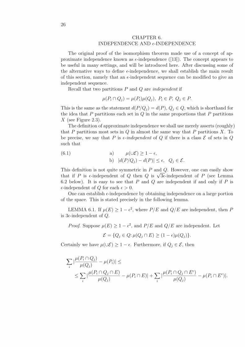
The definition of approximate independence we shall use merely asserts (roughly)that P partitions most sets in Q in almost the same way that P partitions X. Tobe precise, we say that P is ε-independent of Q if there is a class E of sets in Qsuch that

a) µ(∪E) ≥ 1− ε,(6.1)

b) |d(P/Qj)− d(P )| ≤ ε, Qj ∈ E .

This definition is not quite symmetric in P and Q. However, one can easily showthat if P is ε-independent of Q then Q is

√3ε-independent of P (see Lemma

6.2 below). It is easy to see that P and Q are independent if and only if P isε-independent of Q for each ε > 0.

One can establish ε-independence by obtaining independence on a large portionof the space. This is stated precisely in the following lemma.

LEMMA 6.1. If µ(E) ≥ 1− ε2, where P/E and Q/E are independent, then Pis 3ε-independent of Q.

Proof. Suppose µ(E) ≥ 1− ε2, and P/E and Q/E are independent. Let

E = {Qj ∈ Q:µ(Qj ∩ E) ≥ (1− ε)µ(Qj)}.

Certainly we have µ(∪E) ≥ 1− ε. Furthermore, if Qj ∈ E , then

∑i

|µ(Pi ∩Qj)

µ(Qj)− µ(Pi)| ≤

≤∑i

|µ(Pi ∩Qj ∩ E)

µ(Qj)− µ(Pi ∩ E)|+

∑i

|µ(Pi ∩Qj ∩ Ec)

µ(Qj)− µ(Pi ∩ Ec)|.

27

Since P/E and Q/E are independent, the first sum on the right is equal to

∑i

|µ(Pi ∩ E)µ(Qj ∩ E)

µ(Qj)µ(E)− µ(Pi ∩ E)| = µ(E)| Qj ∩ E)

µ(Qj)µ(E)− 1|,

and it is easy to see that the latter quantity cannot exceed ε. Also,

∑i

|µ(Pi ∩Qj ∩ Ec)

µ(Qj)− µ(Pi ∩ Ec)| ≤

≤∑i

µ(Pi ∩Qj ∩ Ec)

µ(Qj)+

∑i

µ(Pi ∩ Ec) =µ(Qj ∩ Ec)

µ(Qj)+ µ(Ec).

If Qj ∈ E , then µ(Qj ∩ Ec) < εµ(Qj), so |d(P/Qj) − d(P )| ≤ ε + ε + µ(Ec) ≤ 3ε.This proves the lemma.

The following lemma shows how one can give a more symmetric definition ofapproximate independence. We prefer to use the more geometric definition ofε-independence given by (6.1).

LEMMA 6.2. If P is ε-independent of Q, then∑i

∑j

|µ(Pi ∩Qj)− µ(Pi)µ(Qj)| ≤ 3ε.

Conversely, if this inequality holds, then P is√

3ε-independent of Q.

Proof. Left to the reader.

We say that a sequence {P i} is an ε-independent sequence if, for each n > 1, P n

is ε-independent of∨n−1

0 P i. The main result of this section is that an ε-independentsequence {T iP} can be modified slightly so as to obtain an independent sequence.To facilitate the statement and proof of this result, we extend the d-metric (definedin Chapter 5 for processes) to arbitrary sequences of partitions. Let P i, 1 ≤ i ≤ n,be a sequence of k set partitions of X, and let P i, 1 ≤ i ≤ n, be a sequence of kset partitions of X. Let Y be a fixed Lebesgue space. Then

dn({P i}ni=1, {P i}ni=1) = inf1

n

n−1∑i=1

|Qi − Qi|,

where this infimum is taken over all sequences Qi, 1 ≤ i ≤ n, and Qi, 1 ≤ i ≤ n,of k set partitions of Y such that

d(n∨1

Qi) = d(n∨1

P i), d(n∨1

Qi) = d(n∨1

P i).

28

Note that dn does not depend on Y . We shall prove

LEMMA 6.3. Let P i, 1 ≤ i ≤ n, and P i, 1 ≤ i ≤ n, be sequences of k setpartitions with the following properties.

a) {P i} is independent.

b) {P i} is ε-independent.

c) |d(P i)− d(P i)| < ε, 1 ≤ i ≤ n.

Then

d) dn({P i}ni=1{P i}ni=1) < 4ε.

Proof. The proof makes use of the fact that a Lebesgue space can be parti-tioned according to any given distribution. We leave to the reader the proof of thefollowing sharper form of this fact.

If P and P are partitions of any two probabilityspaces, and Y is any Lebesgue space, then there arepartitionsQ, Q of Y so that |Q−Q| = |d(P )−d(P )|,d(Q) = d(P ), and d(Q) = d(P ).

(6.2)

This result and condition (c) of the lemma immediately imply that (d) holds forn = 1, so let us assume the lemma is true for n. Suppose {P i} and {P i} satisfy thehypothesis for n + 1. We can apply the induction hypothesis to choose partitionsQi, 1 ≤ i ≤ n, and Qi, 1 ≤ i ≤ n, of a given nonatomic Y so that

i) d(∨n

1 Qi) = d(

∨n1 P

i)

ii) d(∨n

1 Qi) = d(

∨n1 P

i)(6.3)

iii) 1n

∑ni=1 |Qi − Qi| < 4ε.

We will show how to construct Qn+1 and Qn+1 so that (6.3) holds for n+ 1 inplace of n. We shall do this by defining Qn+1 and Qn+1 on the sets A ∩ A, whereA ∈ ∨n

1 Qi, A ∈ ∨n

1 Qi, so that (6.3i) and (6.3ii) will hold for n + 1. We shall use

the hypotheses (a), (b), and (c) to show that the partitioning result (6.2) can beapplied so that (6.3iii) will hold for n+ 1.

First, use (b) to chooses En ⊆∨n

1 Pi such that µ(∪En) ≥ 1− ε and

|d(P n+1/B)− d(P n+1)| < ε, B ∈ En.

The hypotheses (a) and (c) then imply that for B ∈ En and B ∈ ∨n1 P

i the followingholds.

|d(P n+1/B)− d(P n+1/B)| < 2ε.(6.4)

29

Let E∗n denote the sets in∨n

1 Qi that correspond to those in En. Now apply

(6.2) to the space Y = A∩ A, A ∈ E∗n, A ∈ ∨n1 Q

i, and the two partitions P n+1/B,P n+1/B, where B corresponds to A, and B to A. We thus obtain partitionsQn+1/A ∩ A, and Qn+1/A ∩ A so that

i) d(Qn+1/A ∩ A) = d(P n+1/B),

ii) d(Qn+1/A ∩ A) = d(P n+1/B),(6.5)

iii) |Qn+1/A ∩ A− Qn+1/A ∩ A| < 2ε.

If A 6∈ E∗n, we just define Qn+1/A∩ A and Qn+1/A∩ A so that (6.5i) and (6.5ii)hold. The fact that µ(∪E∗n) ≥ 1− ε then tells us that

|Qn+1 − Qn+1| < 4ε,(6.6)

while (6.5i,ii) and (6.3i,ii) imply that

d(n+1∨

1

Qi) = d(n+1∨

1

P i), d(n+1∨

1

Qi) = d(n+1∨

1

P i).(6.7)

This proves the lemma, for (6.6), (6.3ii), and (6.7) combine to show that (d)holds. In fact, we have established a stronger result; namely, that the Qi and Qi

can be chosen so that, for all i, |Qi − Qi| < 4ε. It is enough for later applicationsthat the average given by (d) holds.

The following result is a restatement of these results for gadgets.

LEMMA 6.4. Suppose G = (T, F, n, P ) and G = (T , F , n, P ) are gadgets satis-fying the following conditions:

a) d(∨n−1

0 T−iP/F ) = d(∨n−1

0 T−iP ), d(∨n−1

0 T−iP /F ) = d(∨n−1

0 T−iP ).

b) The seqeunce {T−iP/F} is ε-independent.

c) The sequence {T−iP /F} is independent.

d) |d(P )− d(P )| < ε.

Then

e) dn(G, G) < 4ε.

The above lemma can be restated in terms of the process distance as follows:

LEMMA 6.5. If {T iP} is an ε-independent sequence and {T iP} is an indepen-dent sequence where |d(P )− d(P )| < ε, then d((T, P ), (T , P )) ≤ 4ε.

This can be proved by using the strong form of Rohlin’s Theorem to buildgadgets for T and T of height n which nearly fill the space, then applying Lemma6.4. A direct proof that models the proof given in Lemma 6.3 can be found inChapter 12 (see the proof of Theorem 12.3).

30

CHAPTER 7.ENTROPY

We now introduce the concept of entropy. The entropy of a transformation Trelative to a partition P will be a number H with the property that, for n largeenough, one can use binary strings of length n(H + ε) to code unambiguously P -n-names, except for a collection of P -n-names with total probability less than ε.The development of these ideas is due to C. Shannon in his fundamental paperon information theory ([19]). The existence of such an H was later rigorously es-tablished for ergodic transformations by McMillan ([11]). The entropy H providesthe necessary control over the size of atoms in

∨n−10 T iP . In this chapter, we shall

define the entropy of T relative to P , then calculate it and discuss one form ofMcMillan’s theorem in the case when {T i} is an independent sequence. We shallthen describe some of the general properties of entropy, and establish a theoremrelating ε-independence and entropy. In the next chapter, it will be shown that,if T is fixed, its relative entropy is largest when P is a generator. This will pro-vide an invariant for transformations, and solve part of the isomorphism problem.Our treatment in both sections will omit many proofs. The reader is referred toBillingsley’s excellent book ([3]) for detailed proofs.

Let us begin with the definitions. If P = {P1, P2, . . . , Pk} is a partition, thenthe entropy of P is

H(P ) = −∑i

µ(Pi) log µ(Pi).(7.1)

Any logarithmic base can be used here. We shall always use base 2. The entropyof T relative to P is

H(T, P ) = limn

1

nH(

n∨1

T iP ).(7.2)

It will be shown later that this limit exists.These definitions are most easily understood in the independent case. We first

prove

LEMMA 7.1. If {T iP} is an independent sequence, then H(T, P ) = H(P ).

Proof. To prove the lemma, note that H(P ) depends on the distribution of Pso that H(TP ) = H(P ) if T is a measure-preserving transformation. The lemmais a consequence of this fact and the following result.

If P and Q are independent thenH(P ∨Q) = H(P ) +H(Q).

(7.3)

To prove this, suppose P andQ are independent. Then µ(Pi∩Qj) = µ(Pi)µ(Qj),so that

log µ(Pi ∩Qj) = log µ(Pi) + log µ(Qj).

31

Therefore,

H(P ∨Q) = −∑i,j

µ(Pi ∩Qj) log µ(Pi ∩Qj)

= −∑j

µ(Qj)∑i

µ(Pi) log µ(Pi)

−∑i

µ(Pi)∑j

µ(Qj) log µ(Qj)

= H(P ) +H(Q),

since∑j µ(Qj) = 1 =

∑i µ(Pi).

The result (7.3) immediately implies thatH(∨n

1 TiP ) =

∑ni=1H(T iP ) = nH(P ),

if {T iP} is an independent sequence, hence the lemma is established.

We shall now state a strong form of McMillan’s theorem. We give a proof onlyfor the case when {T iP} is an independent sequence. The general proof can befound in Billingsley ([3], pp. 129ff.).

THE SHANNON-McMILLAN-BREIMAN THEOREM. If T is ergodic, P afinite partition, and ε > 0, there is an N such that, for n ≥ N , there is a collectionEn of atoms in

∨n−10 T iP such that µ(∪En) ≥ 1− ε, and

i) 2−(h(T,P )+ε)n ≤ µ(A) ≤ 2−(h(T,P )−ε)n, for A ∈ En.ii) En contains at least (1− ε)−12(h(T,P )−ε)n and at most 2(h(T,P )+ε)n atoms.

Proof. Note that (ii) is an immediate consequence of (i). To simplify ourdiscussion, we assume that {T iP} is an independent sequence. Suppose A is anatom of

∨n−10 T iP so that A can be uniquely expressed in the form

A =n−1⋂j=0

T jPij .

Let ni = ni(A) be the number of occurrences of Pi in this expression for A; thatis, ni(A) is the number of indices j, 0 ≤ j ≤ n − 1, such that T−jA ⊆ Pi. Theassumption that {T iP} is an independent sequence tells us that

µ(A) = µ(P1)n1µ(P2)n2 . . . µ(Pk)nk .

This can be rewritten in the form

log µ(A) =k∑i=1

ni log µ(Pi).(7.4)

The law of large numbers tells us that, for large n, there is a collection En of atomsof

∨n−10 T iP such that µ(∪En) ≥ (1− ε) and if A ∈ En then

|ni(A)

n− µ(Pi)| ≤ δ, i = 1, 2, . . . , k.

32

If δ is small enough, we combine this with (7.4) to obtain our desired conclusion(i).

To facilitate our further discussion of entropy, we introduce the concept of theconditional entropy of P given Q. This is defined as

H(P |Q) = H(P ∨Q)−H(Q).(7.5)

An easy calculation establishes the formula

H(P |Q) = −∑j

µ(Qj)∑i

µ(Pi ∩Qj)

µ(Qj)log

µ(Pi ∩Qj)

µ(Qj).(7.6)

This shows that H(P |Q) is the average over the atoms of Q of the entropies of theinduced partitions P/Qj.

It was noted above (see (7.3)) that, if P and Q are independent, then H(P ∨Q) = H(P ) + H(Q); that is, H(P |Q) = H(P ). It is also obvious from (7.5) that,if P ⊂ Q, then H(P |Q) = 0. In fact, the formula (7.6) and the strict convexityproperties of x log x imply the converse of these results. In summary,

0 ≤ H(P |Q) ≤ H(P ), with H(P |Q) = 0 if and only if P ⊂ Q,and H(P |Q) = H(P ) if and only if P and Q are independent.

(7.7)

The function H(P |Q) is decreasing in Q and increasing in P ; that is,

a) H(P |Q) ≤ H(P |Q) if P ⊂ P ,(7.8)

b) H(P |Q) ≥ H(P |Q) if Q ⊂ Q.

The definition (7.5) and the results (7.8) enable us to show that limn n−1H(

∨n1 T

iP )indeed exists. First note that H(

∨n+11 T iP ) = H(

∨n0 T

iP ) since T is measure-preserving. Formula (7.5) then gives

H(n∨0

T iP )−H(n∨1

T iP ) = H(P |n∨1

T iP ).

The sequence H(P |∨n1 T

iP ) is decreasing from (7.8)). It is an elementary exerciseto show that, if {an} is an increasing sequence, an ≥ 0, and {an+1 − an} is adecreasing sequence, then {n−1an} converges, and limn−1an = lim(an+1 − an).This then establishes that the limit used in (7.2) actually exists, and furthermorethat

H(T, P ) = limnH(P |

n∨1

T iP ).(7.9)

This result is sometimes summarized by saying that the entropy of T relative to Pis the conditional entropy of the present P relative to the entire past. (Remember

33

that the ith coordinate of the P -name of x is the index of the set in T−iP to whichx belongs.)

We shall later use the following alternative version of (7.9):

(7.9a) H(T, P ) = limnH(P |

n∨1

T−iP ).

This follows from the fact that H(∨n

1 TiP ) = H(

∨n1 T−iP ) since T n+1 is measure-

preserving, and hence H(T, P ) = H(T−1, P ). This with (7.9) establishes (7.9a).Lemma 7.1 asserted that if {T iP} is an independent sequence then H(T, P ) =

H(P ). The converse of this is also true. In summary,

H(T, P ) ≤ H(P ), with equality if and onlyif {T iP} is an independent sequence.

(7.10)

Let us show that {T iP} is indeed an independent sequence if H(T, P ) =H(P ). The hypothesis H(T, P ) = H(P ) combines with (7.9) to tell us thatH(P |∨n

1 TiP ) = H(P ) for n ≥ 1, and hence (7.9) implies that P is indepen-

dent of∨n

1 TiP for n ≥ 1. This proves (7.10). It is important for our later results

that this result has an approximate form.

LEMMA 7.2. Given k and ε > 0, there is a δ = δ(ε, k) > 0 such that if P hask sets and H(T, P ) ≥ H(P )− δ then {T iP} is an ε-independent sequence; that is,for each n, T nP is ε-independent of

∨n−10 T iP .

Proof. Smorodinsky ([22]) showed that δ can be chosen to be independent ofk also. We shall give here the simpler proof of Ornstein for the case when δ isallowed to depend upon k. We first note that (7.9a) gives

H(T nP )−H(T nP |n−1∨

0

T iP ) = H(P )−H(P |n∨1

T−iP ) ≤ H(P )−H(T, P ),

so it is enough to prove the following lemma.

LEMMA 7.3. Given k and ε > 0, there is a δ > 0 such that, if P has k setsand H(P )−H(P/Q) ≤ δ, then P is ε-independent of Q.

Proof of Lemma 7.3. We would like to show that H(P )−H(P |Q) is boundedaway from zero on the set of all pairs (P,Q) such that P has k sets and P is notε-independent of Q. We first show how Q can be replaced by a two set partition.Suppose P has k sets and is not ε-independent of Q, so that the collection E ofatoms A of Q for which

|d(P/A)− d(P )| ≥ ε,

34

has total measure greater than ε. Thus∑i

∑A∈E|µ(Pi ∩ A)− µ(Pi)µ(A)| ≥ ε2,

so that there is a Pi and a subcollection E ′ ⊆ E such that

|∑A∈E ′

µ(Pi ∩ A)− µ(Pi)µ(A)| ≥ ε2/2k.

Let S be the union of the sets in E ′, and note that

µ(S) ≥ ε2/2k and |d(P/S)− d(P )| ≥ ε2/2k.(7.11)

Since S = {S, Sc} is refined by Q, we have H(P |S) ≥ H(P |Q). Furthermore, S isnot independent of P , so that H(P ) > H(P |S). We therefore have

0 < H(P )−H(P |S) ≤ H(P )−H(P |Q).(7.12)

Let K be the set of all (3k + 1)-tuples

d(P ), d(P/S), d(P/Sc), µ(S),

where P is a k set partition and (7.11) holds. The set K is compact, and H(P )−H(P |S) is a continuous non-vanishing function on K, hence it must be boundedaway from 0. This, along with (7.12), shows that Lemma 7.3, and hence Lemma7.2, is true.

If Lemma 7.2 is combined with Lemma 6.4, we obtain the following fundamentalresult.

ORNSTEIN’S COPYING THEOREM. Suppose T is a Bernoulli shift withindependent generator P , where P has k sets. Given ε > 0, there is a δ > 0 suchthat, if T is any ergodic transformation and P any k set partition such that

(i) |d(P )− d(P )| < δand (ii) |H(P )−H(T, P )| < δ,

then(iii) d((T , P ), (T, P )) ≤ ε.

Proof. Given δ′ > 0, if δ is small enough, we have |H(P )−H(P )| < δ′, so that(i) and (ii) will imply that |H(P ) − H(T, P )| < δ + δ′. Thus Lemma 7.2 tells usthat, if δ + δ′ is small enough, {T iP} will then be an ε-independent sequence, sothat, if δ < ε, Lemma 6.4 will imply that d((T , P ), (T, P )) ≤ 4ε. Replace ε by ε/4,and (iii) is then established.

35

The conclusion (iii) of this theorem means that there is a measure-preservingtransformation S from the T -space to the T -space such that, except for a set ofmeasure less than

√ε (which depends on n), the P -n-name of x and the P -n-name

of Sx disagree in less than√εn place. All that is required for this to hold is that the

pair T, P be close enough to the pair T , P in distribution and entropy. This resultwill be very useful in our proof of the isomorphism theorem. Later it will also beshown that, if P is any generator for a Bernoulli shift T , a slightly weaker versionof the copying theorem will hold. This result will, in fact, be the characterization ofBernoulli shifts which enables one to show that many transformations are Bernoullieven when one cannot explicitly construct an independent generator.

36

CHAPTER 8.THE ENTROPY OF A TRANSFORMATION

The entropy H(T, P ) of a transformation T relative to a partition P was definedin the previous section. The number H(T, P ) depends upon the partition P . Toobtain an invariant for T , we define the entropy of T as

H(T ) = sup{H(T, P ): P is a finite partition}.(8.1)

This is clearly an invariant for T ; that is, if S is isomorphic to T , then H(S) =H(T ). At first glance, one might think that H(T ) would always be infinite. Thefollowing result of Komogorov and Sinai ([9], [10], [20]) gives us a means for calcu-lating H(T ), and establishes that H(T ) is finite for a large class of transformations.

KOLMOGOROV-SINAI THEOREM. If P is a generator for T , and Q is anypartition, then H(T, P ) ≥ H(T,Q). In particular, H(T ) = H(T, P ) for any gener-ator P .

Proof. The proof of this result depends upon two lemmas.

LEMMA 8.1. If Q =∨k−k T

iP , then H(T,Q) = H(T, P ).

Proof. We have

H(T,Q) = limnH(Q|

n∨1

T iQ) = limnH(

k∨−kT iP |

n+k∨−k+1

T iP ).

Note that the definition of conditional entropy gives

H(k∨−kT iP |

n+k∨−k+1

T iP ) = H(n+k∨−k

T iP )−H(n+k∨−k+1

T iP ),

which is equal to H(T−kP |∨n+k−k+1 T

iP ). Replace P by T kP to obtain

H(T,Q) = limnH(P |

n+2k∨1

T iP ) = H(T, P ).

This proves Lemma 8.1.

LEMMA 8.2. Given k and ε > 0, there is a δ > 0 such that if P and Q have ksets and |P −Q| ≤ δ then |H(T, P )−H(T,Q)| ≤ ε.

Proof. Fix δ < 1/2, and suppose |P −Q| < δ. Let

R0 =k⋃i=1

Pi ∩Qi, Ri = Pi −R0, 1 ≤ i ≤ k,

37

and letR denote the partition {R0, R1, R2, . . . , Rk}. The strict convexity of−x log x,0 ≤ x ≤ 1, then shows that, for R0 fixed, the largest value of H(R) is obtainedwhen µ(R1) = µ(R2) = . . . = µ(Rk). Thus

H(R) ≤ −δ log δ − (1− δ) log(1− δ) + δ log k,

so we can choose δ so small that H(R) cannot exceed ε. Furthermore, P ∨ Q =Q ∨R, so that

H(T, P ) ≤ H(T, P ∨Q) = H(T,Q ∨R),

and the latter does not exceed H(T,Q) + H(R), so we must have H(T, P ) ≤H(T,Q) + ε. A similar argument shows that, if δ is small enough, then H(T,Q) ≤H(T, P ) + ε, and this completes the proof of Lemma 8.2.

Proof of the Kolmogorov-Sinai Theorem. Suppose P is a generator for T , and Qis some arbitrary finite partition. Given δ > 0, we can find a large k and a partitionQ with the same number of sets as Q, such that Q ⊆ ∨k

−k TiP and |Q − Q| ≤ δ.

This follows from the hypothesis that P is a generator and the assumption that Qhas finitely many sets, for, given any atom A of Q, the set A can be approximatedby sets in the σ-algebra generated by

∨k−k T

iP for large enough k.Since Q ⊆ ∨k

−k TiP , Lemma 8.1 implies that H(T, Q) ≤ H(T, P ), while Lemma

8.2 guarantees that, if δ is small enough, H(T, Q) will be close to H(T,Q). Thuswe must have H(T,Q) ≤ H(T, P ), which completes the proof of the theorem.

If T is a Bernoulli shift, then the Kolmogorov-Sinai Theorem and Lemma 7.1enable one to compute the entropy of T . Suppose P = {P1, P2, . . . , Pk} is a gener-ator for T such that {T iP} is an independent sequence. We then have

H(T ) = −∑

µ(Pi) log µ(Pi).(8.2)

To prove this, use the Kolmogorov-Sinai Theorem to obtain H(T ) = H(T, P ), andthen use Lemma 7.l to obtain H(T, P ) = H(P ).

At this point, note that these results solve part of the isomorphism problem;namely, two Bernoulli shifts cannot possibly be isomorphic unless they have thesame entropy. For example, the Bernoulli shifts T and T , with respective dis-tributions π = (1/2, 1/2) and π = (1/3, 1/3, 1/3), can not be isomorphic forH(T ) = log 2 and H(T ) = log 3.

For any given π = (p1, p2, . . . , pk), there are an uncountable number of distri-butions π = (p1, p2, . . . , pk) such that∑

pi log pi =∑

pi log pi,(8.3)

and the Kolmogorov-Sinai Theorem gives us no positive information about whetherthe two Bernoulli shifts Tπ and Tπ are isomorphic. Meshalkin ([12]) and later Blum

38

and Hanson ([4]) developed special coding techniques for establishing isomorphismswhen, in addition to (8.3), the pi and pj satisfy special algebraic relations. Forexample, Meshalkin showed that, if

π = (1

4,1

4,1

4,1

4) and π = (

1

2,1

8,1

8,1

8,1

8),

Tπ and Tπ are isomorphic.It will be shown in the next two sections that (8.3) is sufficient for isomorphism

of the Bernoulli shifts Tπ and Tπ; that is, entropy is a complete invariant forBernoulli shifts. We sketch here some of the background of the proof of thistheorem.

Suppose T and T are Bernoulli shifts with the same entropy. We can thereforefind generators P and P , respectively, such that {T iP} and {T iP} are each inde-pendent sequences. Furthermore, H(T ) = H(P ) and H(T ) = H(P ), so we musthave H(P ) = H(P ). To prove the isomorphism of T and T , it is enough (fromTheorem 2.1) to find a partition Q such that

a) Q is a generator for T ,(8.4)

b) {T iQ} is an independent sequence,

c) d(Q) = d(P ).

At this point, we mention that Sinai ([20]) showed how to find Q such that (b)and (c) hold. His construction is so difficult that it is not easy to show how onemight choose Q so that (a) will also hold. Ornstein established a much strongerversion of Sinai’s result, showing how one can choose a Q satisfying (b) and (c),which is not too far away from a Q that almost satisfies (b) and (c). Precisestatements of these results are stated here.

SINAI’S THEOREM. If T is a Bernoulli shift with independent generator P ,and if T is any ergodic transformation such that H(T ) ≥ H(T ), then there is apartition Q satisfying

a) {T iQ} is an independent sequence,

b) d(Q) = d(P ).

ORNSTEIN’S FUNDAMENTAL LEMMA. If T is a Bernoulli shift with inde-pendent generator P , and ε > 0, there is a δ > 0 such that, if T is any ergodictransformation with H(T ) ≥ H(T ) and P is any partition with the same numberof sets as P such that

i) |d(P )− d(P )| ≤ δ,

39

ii) 0 ≤ H(T , P )−H(T, P ) ≤ δ,

then there is a partition Q satisfying the following three conditions.

iii) {T iQ} is an independent sequence,

iv) d(Q) = d(P ).

v) |Q− P | ≤ ε.

Note that the fundamental lemma asserts that, once we have found a P satis-fying (i) and (ii), then close to P (in the partition metric) is a partition satisyingconditions (a) and (b) of Sinai’s Theorem. Gadget constructions can be used toobtain partitions satisfying (i) and (ii), hence we can control the location of parti-tions satisfying (iii) and (iv). This will enable us then to modify Q so that it willsatisfy (iii) and (iv) and ”almost” generate, and condition (v) will guarantee thatour sequence of modifications will converge in the partition metric.

The next chapter will contain a proof of the fundamental lemma. The numberδ will come from the copying theorem of Chapter 7; that is, δ will be chosen so that(i) and (ii) guarantee that d((T, P ), (T , P )) is small. This will enable us to copygadgets involving T , P onto those involving T, P and will be the key to controllingthe location of Q. Underlying these constructions will be the following principle.

In order to be certain that H(T,Q) is close to H(T ), choose Q so that,for some n,

∨n−n T

iQ ⊇ Q, where Q is close to a generator P for T .(8.5)

Thus, if |P − Q| ≤ δ and δ is small enough, Lemma 8.2 and the Kolmogorov-SinaiTheorem imply that H(T, Q) will be close to H(T, P ) = H(T ). Lemma 8.1 thenimplies that H(T,Q) ≥ H(T, Q), so H(T,Q) will indeed be close to H(T ).

40

CHAPTER 9.THE FUNDAMENTAL LEMMA

In this section, we shall prove the fundamental lemma. For ease of reference,we restate this result here.

ORNSTEIN’S FUNDAMENTAL LEMMA. If T is a Bernoulli shift with inde-pendent generator P , and ε > 0, there is a δ > 0 such that, if T is any ergodictransformation with H(T ) ≥ H(T ) and P is any partition with the same numberof sets as P such that

i) |d(P )− d(P )| ≤ δ,

ii) 0 ≤ H(T , P )−H(T, P ) ≤ δ,

there is a Q satisfying the following three conditions

iii) {T iQ} is an independent sequence,

iv) d(Q) = d(P ),

and

v) |Q− P | ≤ ε.

In order to facilitate the understanding of the proof of this lemma, we first provea much simpler result, which shows that, for any δ > 0, there is a P satisfying (i)and (ii).

LEMMA 9.1. If T is a Bernoulli shift with independent generator P , and T isany ergodic transformation with H(T ) ≥ H(T ), then, for any given δ > 0, thereis a partition Q with the same number of sets as P such that the following twoconditions hold.

i) |d(Q)− d(P )| ≤ δ,

ii) 0 ≤ H(T , P )−H(T,Q) ≤ δ.

Proof. The key to the proof is the use of gadgets to select new partitions,Lemma 4.2 and the Shannon-McMillan-Breiman Theorem to control entropy, andthe law of large numbers to control the distribution. We first choose a partition Rwith good entropy, that is, so that

0 < H(T , P )−H(T,R) < α,(9.1)

41

where α is a small positive number to be specified later.

The existence of R follows from the fact that H(T,R) is a continuous functionof R in the partition metric, relative to which the set of all partitions is connected.Of course, neither the number of sets nor the distribution of R have any relationto P .

Our goal is to construct a gadget (T, F, n,R) and relabel its columns with P -n-names in such a way that the resulting partition Q satisfies (i) and (ii). Todo this, we need to control the number of columns in the gadget. The Shannon-McMillan-Breiman (SMB) Theorem provides us with this control. Let us writeµ(A) ∼ 2−n(H±ε) if

2−n(H+ε)n ≤ µ(A) ≤ 2−n(H−ε).

Let β be a small positive number to be specified later, and use the SMB theoremto choose n so large that the there is a collection E ⊂ ∨n−1

0 R and a collectionE ⊂ ∨n−1

0 T−1P , each of total measure at least 1− β, such that

(a) µ(A) ∼ 2−n(H(T,R)±β), A ∈ E .

(b) µ(A) ∼ 2−n(H(T ,P )±β), A ∈ E .(9.2)

By choosing β small enough and n large enough, we can assume that

2−(H(T ,P )−β)n ≤ 2−(H(T,R)+β)n.(9.3)

This uses the assumption that H(T,R) < H(T , P ). The inequality (9.3) has theconsequence that, if β is small enough,

There are more sets in E than in E .(9.4)

We can sharpen this result even further by using the law of large numbers. LetfA(i, n) be the relative frequency of i in the P -n-name of the atom A ∈ ∨n−1

0 T−iP .We can assume that n and E satisfy∑

Pi∈P|fA(i, n)− µ(Pi)| ≤ β, A ∈ E .(9.5)

The strong form of Rohlin’s Theorem implies that there is a gadget (T, F , n,R)such that

d(n−1∨

0

T−1R/F ) = d(n−1∨

0

T−iR) and µ(n−1⋃i=0

T iF ) ≥ 1− β.(9.6)

42

We can cut down the number of columns in this gadget by replacing F with F =(∪E)∩ F . Put EF = {A∩ F |A ∈ E}. The conditions (9.6), (9.4), and (9.2a) implythat µ(∪n−1

i=0 TiF ) > 1− 2β, and that there are more sets in E than in EF . Thus

There is a one-to-one function φ from the columns of(T, F, n,R) into the set of P -n-names of the atoms in E .

(9.7)

As in Chapter 4, for A ∈ EF , we label TmA with im, if φ(A) = (i0, i1, . . . , in−1),and let Qi be the union of the sets labelled i. This defines the partition Q on⋃n−1i=0 T

iF , and one can then define Q on the complement of⋃n−1i=0 T

iF in somearbitrary fashion. Let us show that if α and β are small enough and n is largeenough the following hold.

(i) |d(Q)− d(P )| ≤ δ and (ii) 0 ≤ H(T , P )−H(T,Q) ≤ δ.

The fact that (i) will hold follows from (9.5), for, if C is any column of(T, F, n,R), (9.5) implies that∑

i

|µ(Qi ∩ C)− µ(Pi)µ(C)| ≤ βµ(C).

Thus (i) will indeed hold if β is small enough. The proof of (ii) is as follows:Lemma 4.2 implies that, on the set ∪n−1

i=0 TiF , we have

R ⊂n∨−nT i(Q ∨ F), F = {F, F c}.

If β is small enough, there is an

R′ ⊂n∨−nT i(Q ∨ F)

such that R′ is close to R, and hence we can make H(T,R′) close to H(T,R). SinceR′ ⊂ ∨n

−n Ti(Q∨F), we will also have H(T,R′) ≤ H(T,Q∨F), and the latter will

be close to H(T,Q) since H(F) is very small. Thus if n is sufficiently large and αand β are sufficiently small, both (i) and (ii) will hold. This proves Lemma 9.1.

The choice of φ in (9.7) is completely arbitrary. All that is required is that itbe a one-to-one function from the columns of (T, F, n,R) into the set of P -n-namesof atoms in E . Once φ is selected, it determines a Q. If we would like to Q to lieclose to a given P , we need to select φ with some care. The next lemma showsthat, if P has good enough distribution and entropy, then φ can be chosen so thatP -n-names and Q-n-names of most points in the base of the gadget agree in mostplaces. This will imply that P and Q are close.

43

LEMMA 9.2. If T is a Bernoulli shift with independent k-set generator P ,and ε > 0, there is a δ > 0 with the following properties: If T is any ergodictransformation with H(T ) ≥ H(T ), and P is any k-set partition such that

(i) |d(P )− d(P )| ≤ δ, and (ii) 0 ≤ H(T , P )−H(T, P ) ≤ δ,

then, for any δ ≤ 0, there is a k-set partition Q such that

(iii) |d(Q)− d(P )| ≤ δ, (iv) 0 ≤ H(T , P )−H(T,Q) ≤ δ,

and(v) |P −Q| ≤ ε.

Proof. We are going to proceed much as we did in the proof of Lemma 9.1, thenmake use of the gadget metric to copy T , P close to T, P and a marriage lemmato show that φ can be chosen so that Q will be close to P . The number δ comesfrom the Ornstein Copying Theorem in Chapter 7. We use that theorem to findδ > 0 such that, if P satisfies (i) and (ii), then

d((T , P ), (T, P )) < ε,(9.8)

where ε will be specified later.Let T, P be given satisfying (i) and (ii) and hence (9.8). Without loss of gen-

erality, we can also assume that δ < ε. Furthermore, it can be supposed that

0 < H(T , P )−H(T, P ) ≤ δ.(9.9)

If this were not so, we could modify P by a small amount in the σ-algebra gen-erated by

⋃∞−∞{T iP}. Either there will be a modification satisfying (9.9), or all

modifications satisfy H(T , P ) = H(T,Q). In the latter case, we merely choose Qso that (v) holds, and d(Q) = d(P ). This Q would then satisfy (iii) and (iv) forall δ > 0, and we would be finished. Thus we can assume that (9.9) holds.

Now choose R ⊃ P such that

(9.1′) 0 < H(T , P )−H(T,R) < α,

where α is to be specified later. To do this, select R satisfying (9.1), and replaceR by R ∨ P . Continuity of entropy and connectedness of the space of partitionswhich refine P then imply that (9.1′) can be achieved for some R ⊃ P .

Choose β so small and n so large that (9.2), (9.3), (9.4), and (9.5) all hold,then choose (T, F , n,R) such that (9.6) holds. Since R refines P , (9.6) implies

(9.6′) d(n−1∨

0

T−iP ) = d(n−1∨

0

T−iP/F ).

44

Furthermore, each atom A ∈ ∨n−10 T−iR/F ) is contained in a unique atom of∨n−1

0 T−iP ; hence such atoms have P -n-names.

Let F = ∪E ∩ F , F = {A ∩ F |A ∈ E}. As before, µ(⋃n−1

0 T iF ) > 1− 2β, andthere are more atoms in E than in EF . We shall prove that there is a function φsatisfying (9.7) and the following condition.

There is a collection A ⊆ EF , with µ(∪A) ≥ (1− ε/6)µ(F )such that the P -n-name of A ∈ A and the P -n-name ofφ(A) ∈ E disagree in less than ε

6n places.

(9.10)

If (9.10) is true, on each column CA, A ∈ A, there will be at most ε6n indices i

for which Qi ∩ CA 6= Pi ∩ CA, and hence

k∑i=1

µ[(Qi ∩ CA)4 (Pi ∩ CA)] ≤ 2ε

6µ(CA).

It follows that if G =⋃n−1i=0 T

iF then

|Q/G− P/G| ≤ 2ε

3,

and hence |Q − P | will not exceed ε, if 2β < ε/6. Thus once (9.10) is proved,Lemma 9.2 will be established.

To establish (9.10), we make use of the copying condition (9.8). First, choosea gadget (T , F , n, P ) so that

d(n−1∨

0

T−iP /F ) = d(n−1∨

0

T−iP ),

and then (using Lemma 5.4 along with (9.8)) choose P ∗ so that (T, F , n, P ∗) isisomorphic to (T , F , n, P ) and

1

n

n−1∑i=0

|P/T iF − P ∗/T IF | < ε.

Now replace F by F . If β is small enough, we will then have

(a) |d(n−1∨

0

T−iP /F )− d(n−1∨

0

T−iP ∗/F )| < β,(9.11)

(b)1

n

n−1∑i=0

|P/T iF − P ∗/F iF | < 2ε

45

Let E∗F denote the atoms in∨n−1

0 T−iP ∗/F corresponding to those in E . If β issufficiently small, then (9.4) implies that there are more sets in E∗F than in EF . Ourfinal arguments will be simplified if we assume that β is so small that

µ(A) ≥ 4µ(A∗), A ∈ EF , A∗ ∈ E∗F ,(9.12)

so that at least four sets in E∗F are needed to cover a set in EF .Let A be the class of all sets A ∈ EF such that more than half of A is covered

by sets A∗ ∈ E∗F such that the P -n-name of A and the P ∗-n-name of A∗ differ in nomore than n

√2ε place. First, we shall show that ∪A fills up most of F . Towards

this end, let E be the set of points x ∈ F such that the P -n-name and P ∗-n-nameof x disagree in more than n

√2ε places. Lemma 5.1 implies that µ(E) ≤

√2εµ(F ).

Furthermore, if B = ∪E∗F , it follows easily that∑A∈EFA 6∈A

µ(A) ≤ 2[µ(F −B) + µ(E)],

and hence, if ε is small enough and β is small enough, we shall indeed have

µ(∪A) ≥ (1− ε/6)µ(F ).

To complete the proof of (9.10), we make use of Hall’s Matching Lemma (See[6], p. 45). Clearly, the definition of A and property (9.12) imply that any telements A1, A2, . . ., At in A intersect at least t elements in E∗F whose P ∗-n-namediffers from the P -n-name of at least one of the Ai in no more than n

√2ε places.

The marriage lemma thus implies that there is a one-to-one function φ from A toE∗F such that the P -n-name of A ∈ A and the P ∗-n-name of φ(A) differ in no morethan n

√2ε places. Thus defining φ in any arbitrary one-to-one manner on EF −A,

property (9.10) will hold for small ε. The resulting Q will then satisfy (v), for thedistribution of P -n-names is nearly the same as the distribution of P ∗-n-names(from (9.11)). The proof of Lemma 9.1 shows that, if α and β are small enoughand n is large enough, Q will also saitsfy (iii) and (iv). This completes the proofof Lemma 9.2.

Proof of Ornstein’s Fundamental Lemma. Let δ be the number given by Lemma9.2 for ε/2, suppose T is an ergodic transformation with H(T ) ≥ H(T ), and Psatisfies (i) and (ii) of Lemma 9.2. Let δn be the number given by Lemma 9.2 forε/2n, and by induction choose k-set partitions Q(n) such that Q(0) = P and

a) |d(Q(n))− d(P )| ≤ δn+1,

b) 0 ≤ H(T , P )−H(T,Q(n)) ≤ δn+1,

c) |Q(n) −Q(n−1)| ≤ ε/2n.

46

The limiting partition Q = limnQ(n) then satisfies the three conditions

d) d(Q) = d(P ),

e) H(T,Q) = H(T , P ),

f) |Q− P | ≤ ε.

The conditions (d) and (e) imply (see (7.10)) that {T iQ} is an independent se-quence. This completes the proof of the fundamental lemma.

47

CHAPTER 10.THE ISOMORPHISM THEOREM

In this chapter, we shall complete the proof that two Bernoulli shifts with thesame entropy are isomorphic. First, we introduce some convenient shorthand.

If P and Q are partitions, then we write Q ⊂ε P if there is a partition Q ⊂ Pwith the same number of sets as Q such that |Q−Q| ≤ ε.

LEMMA 10.1. P is a generator for T if and only if, for each partition Q andeach ε > 0, there is an n such that Q ⊂ε

∨n−n T

iP .

Proof. To say that P is a generator is to say that, for each set A of positivemeasure and each ε > 0, there is an n and a set B in the σ-algebra generatedby

∨n−n T

iP such that µ(A4 B) ≤ ε. This is easily seen to be equivalent to thelemma.

We shall say that T, P is a copy of T , P , and write (T, P ) ∼ (T , P ) if

d(n∨0

T iP ) = d(n∨0

T iP ), n = 0, 1, 2, . . . .

This means that, for each n, the distribution of P -n-names is the same as thedistribution of P -n-names. Note for example that, if {T iP} is an independentsequence and (T, P ) ∼ (T , P ), then d(P ) = d(P ), and {T iP} is an independentsequence.

Throughout the remainder of this section, T and T will denote Bernoulli shiftswith the same entropy, with respective independent generators P and P . We shallprove

THEOREM 10.1. There is a partition Q such that

i) (T,Q) ∼ (T , P ),

ii) Q is a generator for T .

Theorem 10.1 and the Kolmogorov-Sinai Theorem then imply the Kolmogorov-Ornstein Theorem.

There is no problem constructing Q so that (T,Q) ∼ (T , P ). In fact, one canuse Lemma 9.1 to construct Q′, with d(Q′) very close to d(P ) and H(T,Q′) veryclose to H(T , P ). Then apply Ornstein’s Fundamental Lemma of Chapter 9 toconstruct Q close to Q′ so that (T,Q) ∼ (T , P ). Our goal is to show that such aQ can be modified so that (i) and (ii) of Theorem 10.1 will both hold. We firstintroduce some further notation.

48

The transformation T is defined on (X,Σ, µ) where Σ is generated by the setsin

⋃∞−∞{T nP}. If Q is another partition of X, we let ΣQ denote the complete

σ-algebra generated by⋃∞−∞{T nQ}, and let TQ denote the restriction of T to the

measure space (X,ΣQ, µ). If (T,Q) ∼ (T , P ), then, of course, TQ is a Bernoullishift with independent generator Q. (This is a slight abuse of terminology. Theσ-algebra ΣQ will not, if ΣQ 6= Σ, separate the points of X, so (X,ΣQ, µ) is nota Lebesgue space. Throughout this discussion, we are tacitly making the identifi-cation between sets in ΣQ and their projections onto the factor space (XQ,ΣQ, µ),which is a Legesgue space, defined by ΣQ (see Chapter 1).)

We also need some notation to clarify the relationship between partitions refinedby

∨n−n T

iP and P -names. Suppose P has k sets. The correspondence A↔ {ti(A)}where

A =n⋂−nT iPti

is a one-to-one correspondence between atoms A ∈ ∨n−n T

iP and sequences {ti} ofthe symbols {1, 2, . . . , k} of length 2n+1. (To connect to our prior terminolgy notethat, if sn−i = ti, then {si} is the P -(2n+ 1)-name of T−nA.) The correspondenceA ↔ {ti(A)} induces a correspondence between partitions of (2n + 1)-sequencesand partitions refined by

∨n−n T

iP . Thus, if Π = {Π1,Π2, . . . ,Πm} is a partition of(2n+ 1)-sequences, then Π(P ) = {Π1(P ),Π2(P ), . . . ,Πm(P )} is a partition refinedby

∨n−n T

iP , where Πj(P ) is the union of those atoms A ∈ ∨n−n T

iP such that{ti(A)} ∈ Πj. Furthermore, all partitions refined by

∨n−n T

iP are of this form.We now prove

LEMMA 10.2. Suppose (T,Q) ∼ (T , P ), and let ε > 0. Assume P has k sets.Choose N so that Q ⊂ε

∨N−N T

iP . Then there is a partition P such that

i) (T, P ) ∼ (T, P ),

ii) P consists of sets in ΣQ,

iii) Q ⊂2ε∨N−N T

iP .

In fact, if Π is a partition of (2N + 1)-sequences of {1, 2, . . . , k} such that |Π(P )−Q| ≤ ε, then |Π(P )−Q| ≤ 2ε.

Proof. First, use the fact that P is a generator to choose N1 > N such that

Q ⊂αN1∨−N1

T iP,(10.1)

where α will be specified later. Given n, also to be determined later, apply Rohlin’sTheorem to the transformation TQ to choose a set F ∈ ΣQ such that T iF , 0 ≤ 1 ≤n− 1, is a disjoint sequence and µ(

⋃n−1i=0 T

iQF ) ≥ 1− α.

49

The set F and partition Q give us two isomorphic gadgets. First, we have thegadget (TQ, F, n,Q) which lies in the space (X,ΣQ, µ). Second,since ΣQ ⊆ Σ, wehave the gadget (T, F, n,Q) which lies in the space (X,Σ, µ) . These are clearlyisomorphic, hence we can apply Lemma 4.4 to select a partition P ∗, consisting ofsets in ΣQ such that

(T, F, n,Q ∨ P ) ∼ (TQ, F, n,Q ∨ P ∗),(10.2)

where ∼ indicates gadget isomorphism.This gadget isomorphism forces a number of relations between P and P ∗ to

hold. First, note that, if G =⋃n−1i=0 T

iF , then d(P/G) = d(P ∗/G) so that, if αis small, d(P ) will be close to d(P ∗). Furthermore, suppose Π is a partition of(2N + 1)-sequences such that |Π(P ) − Q| ≤ α. If n is so large that the top andbottom N1-levels of the stack plus the complement of the stack have small measure,then Π(P ∗) will be close to Q. Thus, if α is sufficiently small and n is sufficientlylarge, we will have

|Π(P ∗)−Q| ≤ 2α.(10.3)

The condition (10.3), of course, means that

Q ⊂2α

N1∨−N1

T iP ∗.(10.4)

In particular, if α is small enough, H(T, P ∗) will be very close to H(T,Q) =H(Q) = H(P ) = H(T, P ). In summary, if δ is any given positive number, then αand n can be chosen so that

|d(P ∗)− d(P )| ≤ δ and 0 ≤ H(T, P ∗)−H(P ) ≤ δ(10.5)

Now apply Ornstein’s Fundamental Lemma to TQ to choose δ and then α andn so that there is a partition P , consisting of sets in ΣQ, such that

(a) (T, P ) ∼ (T, P ), and (b) |P − P ∗| ≤ β,(10.6)

where β is a given positive number. If β is small, then (10.6b) will guarantee thatΠ(P ) is close to Π(P ∗), hence β can be chosen so that (10.6b) implies that

|Π(P )−Q| ≤ 2ε.(10.7)

This completes the proof of Lemma 10.2.

50

Lemma 10.2 provides us with a partition which we can copy to show that closeto Q is a copy of (T , P ) that almost generates.

LEMMA 10.3. Suppose (T,Q) ∼ (T , P ). Given ε > 0, there is a partition Qand a number K such that

i) (T, Q) ∼ (T , P ),

ii) P ⊂ε∨K−K T

iQ,

iii) |Q− Q| ≤ ε.

Proof. The idea of the proof is to choose P , consisting of sets in ΣQ, so that(T, P ) ∼ (T, P ), and Q is close to a partition that is refined by

∨K−K T

iP . If K

is large enough then P will be close to a partition that is refined by∨K−K T

iQ.We then construct a long gadget (T, F, n, P ), F ∈ Σ, and an isomorphic gadget(TQ, E, n, P ), E ∈ ΣQ, and use these to construct Q∗ so that (T, F, n, P ∨ Q∗) isisomorphic to (TQ, E, n, P ∨ Q). If this is done carefully, Q∗ will be so close to Qthat the fundamental lemma can be applied to modify it so that the desired Q willexist.

To carry out the above plan, let α be a positive number to be specified later.Choose N1 so that Q ⊂α

∨N1−N1

T iP , then apply Lemma 10.2 to construct a partitionΠ1 of (2N+1)-sequences of {1, 2, . . . , k}, where P has k sets, so that |Π(P )−Q| ≤ α,and a P such that

a) (T, P ) ∼ (T, P ),

b) P consists of sets in ΣQ,

c) |Π1(P )−Q| ≤ 2α.

(10.8)

Since (10.8b) holds, we can choose N2 > N1 so that P ⊂α∨N2−N2

T iQ. Thus thereis a partition Π2 of (2n2 + 1)-sequences of {1, 2, . . . ,m}, where Q has m sets, sothat

|P − Π2(Q)| ≤ α.(10.9)

Now choose N3 > N2 so that P ⊂β∨N3−N3

T iQ, where β will be specified later asa function of α. Hence there is a partition Π3 of (2N3+1)-sequences of {1, 2, . . . ,m}such that

|P − Π3(Q)| ≤ β.(10.10)

Let n be a large number, and use the strong form of Rohlin’s Theorem to chooseF ∈ Σ such that T iF , 0 ≤ i ≤ n− 1, is a disjoint sequence, and

d(n−1∨

0

T−iP/F ) = d(n−1∨

0

T−iP ).(10.11)

51

In a similar manner, choose E ∈ ΣQ such that T iE, 0 ≤ i ≤ n − 1, is a disjointsequence and

(10.11′) d(∨n−1

0 T−iP /E) = d(∨n−1

0 T−iP ).

The condition (10.8a), along with (10.11) and (10.11′), implies that the twogadgets (T, F, n, P ) and (TQ, E, n, P ) are isomorphic. Hence (from Lemma 4.4)there is a Q∗ such that

(T, F, n, P ∨Q∗) is isomorphic to (TQ, E, n, P ∨Q).(10.12)

We shall show that, if β is small enough and n is large enough, then Q∗ can bemodified to obtain the desired Q. First, we can assume that n is so large that thetop and bottom N3-levels of each stack {T iF} and {T iE} plus their complementshave such small measure that (10.10) and (10.12) imply

|Π3(Q∗)− P | ≤ 2β and |d(Q∗)− d(Q)| ≤ 2β,(10.13)

and that (10.12), (10.9), and (10.8c) imply

|Π2(Q∗)− P | ≤ 2α(10.14)

and

|Π1(P )−Q∗| ≤ 3α.(10.15)

If β is small enough, the conditions (10.13) imply that H(T,Q∗) will be veryclose to H(T,Q). Thus we can assume that β is so small that there is a Q satisfying

(a) (T, Q) ∼ (T,Q), (b) |Q−Q∗| ≤ γ(10.16)

Furthermore, if N2 (which does not depend on β) is fixed, we can assume that γis so small that (10.16b) implies that

∨N2−N2

T iQ is very close to∨N2−N2

T iQ∗. Thus,if γ is small enough, this and (10.14) imply that

|Π2(Q)− P | ≤ 3α.(10.17)

Note also that (10.15) and the relation (10.16b) imply that |Π1(P )− Q| ≤ 3α+ γ.Since we started with the hypothesis that |Π1(P )−Q| ≤ α, we therefore can chooseβ so small that

|Q− Q| ≤ 5α.(10.18)

The results (10.16a), (10.17), and (10.18) are the desired results, for we merelyneed to begin with α = ε/5. This proves Lemma 10.3.

52

Proof of Theorem 10.1. First, use Lemma 9.1 combined with Ornstein’s Funda-mental Lemma to select Q(0) so that (T,Q(0)) ∼ (T , P ). Let εn go to zero rapidly,and apply Lemma 10.3 to select Q(n) and Kn such that

a) (T,Q(n)) ∼ (T , P ),

b) P ⊂εn∨Kn−Kn

T iQ(n),(10.19)

c) |Q(n) −Q(n−1)| ≤ εn.

One can clearly assume that the Kn increase. Furthermore, if εn goes to zerofast enough, we can use (10.19c) to assume that

P ⊂εj+...+εn

Kj∨−Kj

T iQ(n+1), 1 ≤ j ≤ n.(10.20)

If we assume that∑εn <∞, then (10.19c) implies that Q = limnQ

(n) exists. Then(10.19a) implies that (T,Q) ∼ (T , P ), while (10.20) will imply that P consists ofsets which are measurable ΣQ. Thus Q will also be a generator. This completesthe proof of Theorem 10.1.

53

CHAPTER 11.FINITELY DETERMINED PARTITIONS

The key result used to prove the isomorphism theorem of Chapter 10 was thelemma that enabled us to modify partitions with good entropy and distributionto obtain arbitrarily better entropy and distribution (Lemma 9.2). There is noreason why one cannot lengthen the gadgets used in this proof so as to obtaingood joint distribution as well. This simple observation is the basis for showing thatmany transformations which arise in other parts of mathematics are isomorphic toBernoulli shifts (see Chapters 12 and 13). In this section, we shall show how tomodify Lemma 9.2 so as to obtain a characterization of generators for Bernoullishifts.

Suppose T is a Bernoulli shift with independent k-set generator P . The prop-erty of the pair T , P used in the proof of Lemma 9.2 was the fact that, if T is anyergodic transformation with H(T ) ≥ H(T , P ) and P is any k-set partition suchthat (a) |d(P )− d(P )| ≤ δ, and (b) 0 ≤ H(T , P )−H(T, P ) ≤ δ, then, if δ is smallenough, we have (c) d((T, P ), (T , P )) < ε. This is the Ornstein Copying Theoremof Chapter 7. This property of an independent generator was used in the proofof Lemma 9.2 to insure that the constructed Q was close to the given P . Thisproperty of independent generators is contained (in a more general form) in thefollowing definition:

Let T be an ergodic transformation and P a k-set partition. We say that P isfinitely determined (relative to T ) if, given ε > 0, there is an n > 0 and a δ > 0such that, if T is any ergodic transformation with H(T ) ≥ H(T , P ) and P is anyk-set partition such that

i) |d(∨n

0 TiP )− d(

∨n0 T

iP )| ≤ δ,

ii) 0 ≤ H(T , P )−H(T, P ) ≤ δ,

then

iii) d((T, P ), (T , P )) < ε.

The Ornstein Copying Theorem asserts that, if {T iP} is an independent se-quence, then P is finitely determined relative to T . As we shall see below, thefinitely determined partitions are precisely those which generate transformationsisomorphic to Bernoulli shifts.

To obtain a stronger version of Lemma 9.2, we need a stronger form of thelaw of large numbers which we now describe. Let (t0, t1, . . . , tm−1) be the P -m-name of an atom of B ∈ ∨m−1

0 T−iP ; that is, B = ∩m−1i=0 T

−iPti . Fix n ≥ m, andlet (s0, s1, . . . , sn−1) be the P -n-name of an atom A ∈ ∨n−1

0 T−iP . Let us use thesymbol fA(B, n) to denote the relative frequency of occurrence of the P -m-name of

54

B in consecutive positions in the P -n-name of A; that is, nfA(B, n) is the numberof indices j, 0 ≤ j ≤ n− 1, such that T jA ⊆ B.

THEOREM 11.1. If T is ergodic, and m and ε > 0 are given, then for allsufficiently large n, there is a collection En of sets in

∨n−10 T−iP of total measure at

least 1− ε such that, for all B ∈ ∨m−10 T−iP and all A ∈ En, we have |fA(B, n)−

µ(B)| ≤ ε.

This is, of course, a simple consequence of the so-called individual ergodictheorem which asserts that for any integrable g and ergodic T ,

limn

1

n

n−1∑i=0

g(T ix) =∫gdµ a.e.

A proof of this ergodic theorem can be found in [3], pp. 20f. We then obtainTheorem 11.1 by letting g be the characteristic function of B, and using the factthat a.e. convergence implies almost uniform convergence (see Egoroff’s Theoremin [8], p. 88).

The following is a general version of Lemma 9.2.

LEMMA 11.1. If P has k sets and is finitely determined relative to T then,given ε > 0, there is an n1 and a δ > 0 such that, if T is any ergodic transformationwith H(T ) ≥ H(T , P ), and P any k-set partition such that

i) |d(∨n1

0 T iP )− d(∨n1

0 T iP )| ≤ δ,

ii) 0 ≤ H(T , P )−H(T, P ) ≤ δ,

then, for any δ > 0 and any n, there is a Q such that

iii) |d(∨n

0 TiQ)− d(

∨n0 T

iP )| ≤ δ,

iv) 0 ≤ H(T , P )−H(T,Q) ≤ δ,

and

v) |P −Q| ≤ ε.

The proof of this lemma is identical to the proof of Lemma 9.2 with threeexceptions. First, we use the definition of finitely determined to choose n1 andδ > 0 such that (i) and (ii) imply that d((T, P ), T , P )) < ε. Second, we must makesure that (ii) can be replaced by

ii’) 0 < H(T , P )−H(T, P ) ≤ δ,

55

so that we can find R ⊂ P for which

0 < H(T , P )−H(T,R) < α

(see statements (9.2) and (9.1’) in the proof of Lemma 9.2). This is proved inLemma 11.2 below. Our third modification in the proof is that we use Theorem11.1 above in place of the law of large numbers to be sure that the class E (see(9.2) ff.) satisfies the property∑

B∈∨n−1

0T iP

|fA(B, n)− µ(B)| ≤ β, A ∈ E .

The constructed Q will then, for suitably small ε and β, satisfy (iii), (iv), and (v).We shall show that we can assume (ii’) holds by showing that, if it cannot be

made to hold, a Q satisfying (iii), (iv), and (v) can be constructed directly fromthe definition of finitely determined partition. Let T , P be finitely determined,let ε be a positive number, and choose n1 and δ so that, if (i) and (ii) hold, thend((T, P ), (T , P )) < ε. Let T, P be given, satisfying (i) and (ii).

LEMMA 11.2. Suppose that H(T,Q) ≥ H(T , P ) for any k-set partition Q forwhich |Q− P | < 2ε. Then given n and δ > 0, there is a Q satisfying (iii) and (iv)of Lemma 11.1, and |Q− P | < 2ε.

Proof. Given α > 0, use Lemma 5.4 to choose gadgets G = (T, F, n, P ) and G =(T , F , n, P ) so that µ(

⋃n−1i=0 T

iF ) ≥ 1− α, µ(⋃n−1i=0 T

iF ) ≥ 1− α, and dn(G, G) < ε.Thus we can choose Q so that

G is isomorphic to (T, F, n, Q)(11.1)

and1

n

n−1∑i=0

|P/T iF −Q/T iF | < ε.(11.2)

If α ≤ ε, condition (11.2) implies |Q − P | < 2ε, so that our hypothesis impliesthat H(T,Q) ≥ H(T , P ). We can choose Q in the σ-algebra generated by P underT , and so obtain H(T,Q) ≤ H(T, P ) ≤ H(T , P ) and therefore be sure that (iv)holds. If α ≤ δ/2, we also obtain (iii) from condition (11.1). This completes theproof of Lemma 11.2, and thus Lemma 11.1 is established.

Ornstein’s Fundamental Lemma in the following general form follows easilyfrom Lemma 11.1.

ORNSTEIN’S FUNDAMENTAL LEMMA (GENERAL FORM). If P and Tare as in Lemma 11.1, then, given ε > 0, there is an n1 and a δ > 0 such that, ifT is any ergodic transformation satisfying H(T ) ≥ H(T , P ), and P is any k-setpartition satisfying

56

i) |d(∨n1

0 T iP )− d(∨n1

0 T iP )| ≤ δ,

ii) 0 ≤ H(T , P )−H(T, P ) ≤ δ,

then there is a Q such that

iii) d(∨n

0 TiQ) = D(

∨n0 T

iP ), n = 0, 1, 2, . . . ,

iv) |P −Q| ≤ ε.

The Ornstein isomorphism theorem (Theorem 10.1) now extends to the follow-ing result.

THEOREM 11.2. Any two transformations T and T with finitely determinedgenerators P and P are isomorphic if they have the same entropy; that is, there isa Q such that

i) (T,Q) ∼ (T , P ),

ii) Q is a generator for T .

This is proved in much the same way as the isomorphism theorem (Theorem10.1). The only change which is needed in that proof is to choose gadgets longenough so that one gets good joint distributions for large n1, so that one can applythe general form of the Fundamental Lemma above. We leave the details to thereader.

We complete this chapter by proving

THEOREM 11.3. If P is a generator for a Bernoulli shift T , then P is finitelydetermined.

Proof. Once can actually prove that any partition P for a Bernoulli shift isfinitely determined ([14]). The proof of this is quite complicated. We give here thesimpler proof for the case when P is a generator (in fact, all that is used about Pis that H(T , P ) = H(T ).

Let B be an independent generator for T , and assume P is a k-set generator.Fix δ and n1 (to be specified later), and suppose T is an ergodic transformationwith H(T ) ≥ H(T ), and that P is a k-set partition such that

i) |d(∨n1

0 T iP )− d(∨n1

0 T iP )| ≤ δ,

ii) 0 ≤ H(T , P )−H(T, P ) ≤ δ.

We wish to show that, if δ is small enough and n1 is large enough, then

57

iii) d((T, P ), (T , P )) < ε.

This will be accomplished by choosing a copy T,B of T , B so that P -namesare related to B-names in (almost) the same way that P -names are related to B-names. Let α and α1 ≤ α be positive numbers to be specified later, and choose Nand N1 ≥ N so that

N∨−N

T iB ⊂α P andN1∨−N1

T iB ⊂α1 P .(11.3)

Then construct gadgets (T , F , n1, P ) and (T, F, n1, P ) so that

d(n1−1∨

0

T−iP ) = d(n1−1∨

0

T−iP/F ),(11.4)

d(n1−1∨

0

T−iP ) = d(n1−1∨

0

T−iP /F ),

and, for each gadget, the complement and top and bottom N1-levels contain lessthan α1 of the space. If δ is small enough, equation (11.4) and condition (i) implythat we can choose F ∗ ⊂ F , F ∗ ⊂ F so that

(T, F ∗, n1, P ) ∼ (T , F ∗, n1, P ),(11.5)

and µ(F−F ∗), µ(F−F ∗) are both very small, and ∼ indicates gadget isomorphism.Now Lemma 4.4 is used to select B∗ so that

(T , F ∗, n1, P ∨ B) ∼ (T, F ∗, n1, P ∨B∗).(11.6)

If n1 is large enough and δ is small enough, the conditions (11.6) and (11.3)guarantee

N1∨−N1

T iB∗ ⊂3α1 P andN∨−N

T iB∗ ⊂3α P,(11.7)

since we have assumed that α1 ≤ α. Thus in particular, we can choose α1 so thatd(B∗) is close enough to d(B), and H(T,B∗) is close enough to H(T , B) so we canapply Ornstein’s Fundamental Lemma to obtain B such that

(T,B) ∼ (T , B) and |B −B∗| < β,(11.8)

where β is any quantity specified in advance. If β is small enough, we can be surethat

|N∨−N

T iB −N∨−N

T iB∗| < α,(11.9)

58

and hence (11.7) givesN∨−N

T iB ⊂4α P.(11.10)

Let S be the measure-preserving transformation which carries T,B onto T , B.The conditions (11.3) and (11.10) then give |SP − P | ≤ 5α, so, if α < ε/5, weobtain the desired inequality

d((T, P ), (T, P )) < ε.

This completes the proof of Theorem 11.3.The reader is referred to [16] for a further discussion of the d-metric and the

concept of finitely determined partition.

59

CHAPTER 12.WEAK AND VERY WEAK BERNOULLI PARTITIONS

The results of Chapter 11 can be used to show that many transformationsof physical and mathematical interest are isomorphic to Bernoulli shifts. This isusually done by showing that there is a generating partition which satisfies somecondition that implies that it is finitely determined. Two such conditions arediscussed in this section, each presented in the context of a specific example.

A class of transformations of interest are the Markov shifts. These are theshifts associated with stationary Markov chains, and are defined as follows: Let Πbe a k × k-matrix with nonnegative entries, each row of which has sum 1, and letπ be a k-tuple of nonnegative numbers which sum to 1. The space X is the setof doubly infinite sequences of the symbols 1, 2, . . . , k, and the measure µ is theunique complete extension of the measure defined on cylinder sets by the formula

µ{x|xi = ti, −m ≤ i ≤ n} = πt−mΠt−mt−m+1 . . .Πtn−1tn .(12.1)

We also assume that πΠ = Π, from which it follows that the shift T defined by(Tx)n = xn+1, n = 0,±1,±2, . . ., is µ-invariant. T is called the Markov shift withinitial distribution π and transition matrix Π.

The reader is referred to Billingsley’s book [3] for a discussion of the propertiesof Markov shifts. For our purposes, we are interested in the following. Let E be thek × k-matrix each row of which is π. Then we have ΠE = EΠ = E. Furthermore,

T is mixing iff limn

(Πn − E) = 0.(12.2)

The following result, due to Friedman and Ornstein ([5]), was the first general-ization of the original isomorphism paper ([13]).

THEOREM 12.1. A mixing Markov shift is isomorphic to a Bernoulli shift.

Except in a few cases, it is very difficult to construct a generator for a Markovshift whose iterates are independent. It is fairly easy, however, to find a generatorthat satisfies an asymptotic condition which implies it is finitely determined. Thisgenerator is the partition P = {P1, P2, . . . , Pk}, where

Pi = {x|x0 = i}.(12.3)

It is obvious that P is a generator for T . We shall prove that P is weak Bernoulli,a concept defined as follows: a partition P is called weak Bernoulli for an ergodictransformation T if, given ε > 0, there is an N such that, for all m ≥ 1,

0∨−m

T iP is ε-independent ofN+m∨N

T iP.

60

For the process T, P , this says that the future and distant past are approximatelyindependent, and is a strong form of the well known Kolmogorov 0− 1 law, whichstates that any set measurable with respect to the arbitrarily distant past hasmeasure 0 or 1. If P is weak Bernoulli, then the process T, P certainly satisfies the0− 1 law, but the converse of this is false ([17]).

Later in this chapter, it will be shown that a weak Bernoulli partition is finitelydetermined. At this point, we shall show that the partition P of (12.3) is weakBernoulli for a mixing Markov shift. Towards this end, fix m and N , and letA ∈ ∨0

−m TiP , B ∈ ∨N+m

N T iP so that A and B have the form

A = Pt0 ∩ T−1Pt−1 ∩ . . . ∩ T−mPt−m , B = TNPtN ∩ . . . ∩ TN+mPtN+m.

The formula (12.1) then gives

µ(A ∩B) =∑tN−11

πt−mΠt−mt−m+1 . . .ΠtN+m−1tN+m,

where the sum is taken over all possible (N − 1)-tuples tN−11 = t1, . . . , tN−1 of the

symbols 1, 2, . . . , k. It is easy to see that∑t1,...,tN−1

Πt0t1 . . .ΠtN−1tN = Π(N)t0tN ,

where (Π(N)ij ) is the N th power of Π. We also have

µ(A)µ(B) = πt−mΠt−mt−m+1 ..Πt−1t0πtN ΠtN tN+1..ΠtN+m−1tN+m

so that

µ(A ∩B)− µ(A)µ(B) = µ(A)[Π(N)t0tN − πtN ]ΠtN tN+1

. . .ΠtN+m−1tN+m,

from which it easily follows that

∑A,B

|µ(A ∩B)− µ(A)µ(B)| ≤k∑

i,j=1

|Π(N)i,j − πj|,

where the left-hand sum is taken over all A ∈ ∨0−m T

iP and all B ∈ ∨N+mN T iP .

Mixing then implies (from 12.2) that, uniformly in m,

limN→∞

∑A,B

|µ(A ∩B)− µ(A)µ(B)| = 0,

and this implies (see Lemma 6.2) that P is indeed weak Bernoulli. Thus Theorem12.1 is established once we have proved the following.

61

THEOREM 12.2. A weak Bernoulli partition is finitely determined.

This can be proved by generalizing the proof that a partition with independentiterates is finitely determined (Ornstein’s Copying Theorem, Chapter 7). We shalldescribe instead a weaker condition (called ”very weak Bernoulli”), and give aproof later that very weak Bernoulli implies finitely determined.

The definition of very weak Bernoulli is given in terms of the extension of thed-metric to arbitrary sequences of partitions, as discussed in Chapter 7. Let {P i}and {P i} be two finite sequences of k set partitions. Then

dn({P i}n−1i=0 , {P i}n−1

i=0 ) = inf1

n

n−1∑i=0

|Qi − Qi|,

where this infinum is taken over all sequences {Qi}n−1i=0 and {Qi}n−1

i=0 of k-set parti-tions of a given Lebesgue space X that satisfy

d(n−1∨

0

P i) = d(n−1∨

0

Qi), d(n−1∨

0

P i) = d(n−1∨

0

Qi).

A partition P is called very weak Bernoulli for T if, given ε > 0, there is an Nsuch that, for all m > 0,

dN({T iP/A}N−1i=0 , {T iP}N−1

i=0 ) < ε

for all atoms A in a collection Am of atoms in∨−1−m T

iP of total measure at least1 − ε. This says (roughly) that, for each m > 0, one can, for most atoms A (inthe past) find a measure-preserving transformation S from A into the whole spacesuch that, for most points x ∈ A, the P -N -name of x and the P -N -name of Sxagree in most places.

It is easy to see that weak Bernoulli implies very weak Bernoulli. Later we showthat very weak Bernoulli implies finitely determined (see Theorem 12.3 below).The concept of very weak Bernoulli was introduced by Ornstein ([15]) as an aid inshowing that a Bernoulli shift can be embedded in a flow. We shall at this pointsketch this proof as it illustrates the kind of argument which is used in the proofsthat many other transformations are Bernoulli.

Let S denote the Bernoulli shift on the unit interval X, with a 2-set independentgenerator Q = {Q0, Q1} satisfying µ(Q0) = µ(Q1) = 1/2. Let f be defined by

f(x) =

{1 if x ∈ Q0

α if x ∈ Q1,

where α is a fixed irrational larger than 1. X will denote the space {(x, y)|x ∈X, 0 ≤ y ≤ f(x)}, with Lebesgue measure (normalized so that µ(X) = 1). A flow

62

{Tt} is defined on X as follows: A point on the fiber with base x moves upwardswith uniform speed until it hits the graph of f . It then moves instantaneously tothe fiber with base Sx and continues moving at uniform speed (see Figure 12.1).

-

?

�

6

z

T 12(z)

•

•

6

•T 32(z)

Sx x• •Q0 Q1

1

α

Figure 12.1

The flow {Tt} is called the flow with base S built under the function f . Clearly,{Tt} is a one-parameter group of measure-preserving transformations on the Lebesguespace X. More general flows can be constructed by using a more general base trans-formation and function f . In fact, Ambrose ([11]) showed that every ergodic flow isisomorphic to a flow built under some function. (See Totoki ([23]) for a discussionof properties of such flows, including the flow of Figure 12.1.)

Let P denote the two-set partition of X given by

P0 = {(x, y)|x ∈ Q0}, P1 = {(x, y)|x ∈ Q1}.(12.4)

We shall prove that each member Tt, t 6= 0, is isomorphic to a Bernoulli shift. Thiswill be done in three stages. First, it will be shown that P is a generator for Tγif 0 < γ < 1/4. Second, it will be shown that P is very weak Bernoulli for anyTγ, γ 6= 0. Third will come the proof that very weak Bernoulli implies finitelydetermined. This will prove that each Tγ, 0 < γ < 1/4, and hence that each Tt,t 6= 0, is isomorphic to a Bernoulli shift.

An extension of our terminology will be helpful in these proofs. If z = (x, y),then the continuous P -name of z is the partition of the real line into the two sets

P0(z) = {t| Ttz ∈ P0}, P1(z) = {t| Ttz ∈ P1}.

63

Note that P0(z) is a countable disjoint union of intervals of integer lengths, andP1(z) is a countable disjoint union of intervals whose lengths are integer multiplesof α. Also note that Pi(Ttz) = −t + Pi(z). The ergodic theorem (Theorem 11.1)applied to the base transformation S implies that, for almost all points z, allpossible finite sequences of intervals occur in the continuous name of z. To makethis precise, let ni, 0 ≤ i ≤ k, and mi, 0 ≤ i ≤ k, be sequences of positive integerssuch that n0 = m0 and define the two sequences

u` =∑i=0

ni + α∑i=0

mi, 0 ≤ ` ≤ k,

v` = n`+1 + u`, 0 ≤ ` ≤ k − 1.

We then have the following.

There is a null set E ⊂ X such that if z 6∈ E, then there is a tsuch that for any k and {ni}, {mi} the intervals (u`, v`+1) belongto P0(Ttz) and the intervals (v`, u`+1) belong to P1(Ttz).

(12.5)

Clearly, two distinct points z and z will have distinct continuous P -names. Wewould like to show that, if γ is fixed, 0 < γ < 1/4, and T = Tγ, then distinctpoints will have distinct discrete T -P -names. This is easy to show (since γ ≤ 1/4)if z = (x, y), z = (x, y), and x 6= x, for then x and x have sistinct S-Q-names.Let us suppose that z = (x, y), z = (x, y), and that y − y = δ > 0. We alsosuppose z 6∈ E, where E is the set of measure zero of (12.5). We now make use ofthe following elementary result (whose proof is left to the reader; see also [3], pp.15-16).

If α1/α2 is irrational, and (·) denotes fractional part, thenumbers (nα1 +mα2), n,m positive integers,are dense inthe unit interval.

(12.6)

Choose a positive integer k such that γ/k < δ, then use (12.6) to choosesequences n`, m`, 1 ≤ ` ≤ k, such that

`− 1

k≤

∑i=1

ni/γ +l∑i=1

miα/γ

≤ `

k.(12.7)

64

C

C

B t

Q0 Q1

1

α

Figure 12.2

δ

R

Q0 Q1

Approximately thesame proportion ofTNγ B lies in each δrectangle

1

α

Figure 12.3

x

(x, y1)

(x, y2) (x, y)R·t2

t1@I

�@R

1

α

Figure 12.4

65

Choose t for z from the result (12.5), and choose n such that nγ − t = γ′,where 0 < γ′ ≤ γ. From (12.7), we have that there is an `, 1 ≤ ` ≤ k, such that|γ′ − w`γ| < δ, where w` = (

∑ni/γ +

∑miα/γ), and this tells us that there is an

integer K such that Kγ + δ ∈ P0(z) while Kγ ∈ P1(z). Since P0(z) = δ + P0(z),we therefore have T kz ∈ P1 and T kz ∈ P0. This completes the proof that P is agenerator for T .

Now for a sketch of the proof that P is very weak Bernoulli for each Tγ, γ 6= 0.Fix γ 6= 0, and put T = Tγ. Let C ∈ ∨−1

−k SiQ, and suppose C ⊂ P1. Fix t,

0 < t < α, and put C = TtC, B = TtQ1 (see Figure 12.2). We assert that for alln ≥ 0

d(n∨0

T iP/C) = d(n∨0

T iP/B).(12.8)

This follows from the fact that each time we go through the top in Figure 12.2, apast set in the base is split into two parts of equal size, one of which goes to theleft half, the other to the right half.

We next make the observation that, for some large N , the set TN B is nearlyuniformly distributed throughout the space; that is, given δ > 0 and a subdivisioninto rectangles of height δ (or very close to δ) as shown in Figure 12.3, there is anN such that TN B appears in nearly the same (linear) proportion in each rectangle.This follows from the renewal theorem ([2], p. 219) applied to the random walkswith jump ahead of 1 or α, each with probability 1/2. It will be assumed that suchan N has been selected.

Consider one of the rectangles R of Figure 12.3, say one on the right-hand side.The intersection TN B ∩ R is made up of translates upwards of past (relative toN) atoms from the base; that is, TN B ∩ R is a union of sets TtA, where A is anatom of some

∨nk S

iQ, n ≤ N . Fix such an A, and put Bt = TtQ1. Choose t1, t2so that Tt1Q1 and Tt2Q1 are the bottom and top, respectively, of R. We then havet1 < t < t2, |t1 − t2| ≤ δ. Let (x, y) ∈ Bt, (x, y1) ∈ Tt1Q1, (x, y2) ∈ Tt2Q1 (seeFigure 12.4). If δ is small, the T, P -names of (x, y1) and (x, y2) can differ only ina few places; that is, one can choose δ so small that for m ≥ 1

dm({T iP/R}i=N+mi=N+1 , ({T iP/Bt}i=N+m

i=N+1 ) ≤ ε.(12.9)

The uniform distribution of T nB and the result (12.8) then imply that, for all nlarge enough,

dn({T iP}n−1i=0 , {T iP/C}n−1

i=0 ) ≤ ε

for all atoms C ∈ ∨−1−k S

iQ and for all k ≥ 1. Simple integration establishes that Pis indeed very weak Bernoulli for T . The existence of a Bernoulli flow is thereforea consequence of the following theorem.

THEOREM 12.3. A very weak Bernoulli partition is finitely determined.

66

Proof. The proof of this is obtained by extending as much as we can the ideasused in the proof that an independent generator is finitely determined (see theOrnstein Copying Theorem, Chapter 7). Our first task is to sharpen Lemma 7.2.Let P be very weak Bernoulli for T . Given ε > 0, choose N so that, for eachm > 0, there is a collection Em of atoms of

∨−1−m T

iP of total measure at least 1− εsuch that, for A ∈ Em,

dN({T iP /A}N−1i=0 , {T iP}N−1

i=0 ) < ε.(12.10)

We would like now to show that, if T, P is close enough to T , P in joint distri-bution and entropy, then a result analogous to (12.10) will hold. This is

LEMMA 12.1. If T , P and N are as above, there is a δ > 0 and an n∗ such thatif T is any ergodic transformation with H(T ) ≥ H(T P ), and P is any partition(with the same number of sets as P ) such that

i) |d(∨n∗

0 T iP )− d(∨n∗

0 T iP )| ≤ δ,

ii) 0 ≤ H(T , P )−H(T, P ) ≤ δ,

then, for each m > 0, there is a class Em ⊂∨−1−m T

iP of measure at least 1 − 3εsuch that, for A ∈ Em,

iii) dN({T iP/A}N−1i=0 , {T iP}N−1

i=0 ) ≤ 3ε.

Proof. One can easily generalize Lemma 7.3 to see that there is a δ = δ(ε, k) > 0so that, if P is any k-set partition, and Q and R are any partitions satisfying

H(P |Q)−H(P |Q ∨R) ≤ δ,(12.11)

then there is a class E ⊂ Q of measure at least 1 − ε such that, for A ∈ E , thepartitions P/A and R/A are ε-independent. We then select n so large that

H(N−1∨

0

T iP |−1∨−nT iP ) < NH(T , P ) + εδ,(12.12)

where δ = δ(ε, k), and k is chosen to be kN ; k = number of sets in P . Now chooseδ so that (i), with n∗ = n, implies that there is a class En ⊂

∨−1−n T

iP of measureat least 1− ε such that, for A ∈ En, we have

dN({T iP/A}N−1i=0 , {T iP}N−1

i=0 ) < ε.(12.13)

Certainly (iii) now holds for m ≤ n. If m > n, the condition (ii) is used. If δ issmall enough, (12.12) and conditions (i) and (ii) imply that

H(N−1∨

0

T iP |−1∨−nT iP ) < NH(T, P ) + εδ.

67

This and condition (ii) now guarantee that, for all m ≥ n,

H(N−1∨

0

T iP |−1∨−nT iP )−H(

N−1∨0

T iP |−1∨−m

T iP ) ≤ δ(12.14)

since, for any T, P,m, we always have NH(T, P ) ≤ H(∨N−1

0 T iP |∨−1−m T

iP ).Fix m > n, and use (12.11) with P replaced by

∨N−10 T iP , Q replaced by∨−1

−n TiP , and R replaced by

∨−n−1−m T iP . Thus (12.11) and (12.13) imply that

there is a class En ⊂ Q of measure at least 1 − 2ε such that (12.13) holds forA ∈ En, and the partitions

∨N−10 T iP/A and

∨−n−1−m T iP/A are ε-independent. It

is easy to see that this implies that (iii) holds, so the proof of Lemma 12.1 iscompleted where n∗ = n+N .

Proof of Theorem 12.3 (continued). The remainder of the proof of Theorem12.3 is very similar to the proof of Lemma 7.3. Suppose P is very weak Bernoullifor T , and ε > 0. Choose N so that (12.10) holds; then choose δ > 0 and n∗ fromLemma 12.1. Let T be an ergodic transformation such that H(T ) ≥ H(T , P ), andlet P be a partition so that (i) and (ii) of Lemma 12.1 hold. We shall show howto construct partitions {Qi}, {Qi} of a Lebesgue space X so that for all n ≥ 0

a) d(n−1∨i=0

Qi) = d(n−1∨

0

T iP ), d(n−1∨

0

Qi) = d(n−1∨

0

T iP ),(12.15)

b)1

n

n−1∑i=0

|Qi − Qi| ≤ 13ε.

This will establish the desired conclusion that conditions (i) and (ii) of Lemma12.1 imply that d((T, P ), T , P )) < 13ε.

In the proof of Lemma 7.3, we constructed the desired Q’s one step at a time.Here we do it N steps at a time. One can certainly choose Q0 and Q0 by assumingthat δ < 13ε and n∗ > 0. Suppose we have found sequences Qi and Qi, 0 ≤ i ≤m − 1, so that (12.15) holds for n = m. The hypothesis (12.10) and the result(iii) of Lemma 12.1 then imply that there is a class Em ⊂

∨m−10 T iP and a class

Em ⊂∨m−1

0 T iP so that µ(∪Em) ≥ 1− 3ε, µ(∪Em) ≥ 1− ε, and

dN({Tm+iP/B}N−1i=0 , {tm+1p/B}N−1

i=0 ) < 5ε,(12.16)

for all B ∈ Em, B ∈ Em; provided we choose δ < ε.Let A be the set in

∨n−10 Qi corresponding to B ∈ ∨n−1

0 T iP , and let A be theset in

∨m−10 Qi corresponding to B ∈ ∨m−1

0 T iP under the correspondence given by(12.15a). The result (12.16) implies that, on the Lebesgue space A∩A where B ∈ E ,

68

B ∈ Em, we can construct partitions Qi/A∩ A and Qi/A∩ A, m ≤ i ≤ m+N − 1,so that

d(m+N−1∨

m

Qi/A∩ A) = d(m+N−1∨

m

T iP/B),

d(m+N−1∨

m

Qi/A ∩ A) = d(m+N−1∨

m

T iP /B)

(12.17)

and1

N

m+N−1∑i=m

|Qi/A ∩ A− Qi/A ∩ A| < 5ε.(12.18)

For those sets A ∩ A, for which the corresponding B is not in Em or the corre-sponding B is not in Em, we merely define Qi/A∩ A and Qi/A∩ A so that (12.17)holds. This will guarantee that (12.15a) holds for n = m + N . The fact that(12.18) holds and that µ(∪Em) ≥ 1− 3ε, µ(∪Em) ≥ 1− 3ε then imply that

1

N

m+N−1∑i=m

|Qi − Qi| < 13ε,

and this certainly implies that (12.15b) holds for n = m+N . This completes theproof of Theorem 12.3.

69

CHAPTER 13.FURTHER RESULTS AND QUERIES

We list here a number of recent results which make use of the ideas describedin this work. We also list some open questions.

1. K-AUTOMORPHISMS. A natural generalization of the class of Bernoullishifts is the class of Kolmogorov or K-automorphisms. T is a K-automorphism ifit has a generator P such that every set in the tail field ∩nΣn has measure 0 or 1,where Σn is the σ-algebra generated by ∪i≥nT iP .

An alternative definition of K-automorphisms is due to Rohlin and Sinai ([45]).T is a K-automorphism if H(T, P ) > 0 for every nontrivial partition P . ThusK-automorphisms are completely nondeterministic in the sense that no nontrivialpartition is measurable with respect to its past.

The significance of K-automorphisms is due primarily to the work of a num-ber of Russian authors in the 1960’s, who established that many transformationsof physical and mathematical interest are K-automorphisms. These include theclass of ergodic (group) automorphisms of separable compact groups, the so-calledAnosov diffeomorphisms, geodesic flow on manifolds of constant negative curva-ture, and the flow associated with the hard sphere gas (see the references in [48],[36]). Much effort has gone into the problem of showing that these transforma-tions are actually Bernoulli shifts, particularly after it was shown that not everyK-automorphism is Bernoulli ([17]). We describe here some of the results whichhave been obtained.

Adler and Weiss in [26] showed that an ergodic automorphism of the torus (i.e.,the product of two circles) is a mixing Markov shift. The results of Chapter 12therefore imply that these are Bernoulli. Katznelson ([31]) used Fourier approxi-mation methods to show that, if T is an ergodic automorphism of the n-torus (theproduct of n circles), then T is Bernoulli. This is done by taking a partition Pinto rectangles, then approximating the characteristic function of a set A in P bya Fejer polynomial. In this way, one can show that given ε > 0 and M , there is anN such that, for all m > 0,

∨−1−m T

iP is ε-independent of∨N+N2

N T iP .

This condition is slightly weaker than weak Bernoulli, but it is easy to see thatit implies very weak Bernoulli. The proof of Katznelson’s theorem is completed byusing the following result of Ornstein (see [14]).

THEOREM 13.1. If {Σn} is an increasing sequence of σ-algebras which areinvariant under T and T−i, and the restriction of T to each Σn is Bernoulli, thenT is Bernoulli on the join of the Σn.

The above results have been modified slightly in an unpublished work of Katznel-son and Weiss to show that an ergodic automorphism of a solenoidal group (i.e., a

70

group whose dual is a subgroup of the rationals) is Bernoulli. It remains an openquestion whether these results can be extended to arbitrary compact groups.

An Anosov or C-diffeomorphism is a diffeomorphism of a manifold with asmooth invariant measure which has foliations into expanding and contractingdirections (see [27], pp. 53f). The horizontal and vertical foliations of a Baker’stransformation can be regarded, respectively, as expanding and contracting folia-tions. The existence of such foliations has been exploited to establish that suchtransformations are Bernoulli. The recent paper of Ornstein and Weiss ([44]) hasan extensive discussion of this foliation property, using it to prove that geodesicflow on a manifold of negative curvature is Bernoulli.

Transformations associated with other physical models such as the Ising modelare of interest. Gallavotti ([30]) has shown that the shift in the one-dimensionalmodel with finite first moment is Bernoulli, and has utilized the recent results oncommuting families ([32]) to show that certain two-dimensional shifts are Bernoulli.These results are clearly only a beginning.

The problem of classifying K-automorphisms is completely open. It is knownthat there is an uncountable family of nonisomorphic K-automorphisms with thesame entropy ([17]), and that there exists a K-automorphism with no square root([39]), and a K-automorphism with no roots at all (unpublished work of J. Clark).It is possible that the rigid block structure of the family in [17] will form the basisfor further invariants.

If Σ′ is a sub-σ-algebra invariant under T and T−1, the transformation T on thespace (X,Σ′, µ) is called a factor of T , and Σ′ is called a factor algebra of T . If T isa K-automorphism, then T has Bernoulli factors of full entropy (this follows fromSinai’s Theorem, Chapter 9), and hence Theorem 13.1 above implies that T hasmaximal Bernoulli factors of full entropy. It is unlikely that such maximal factorsare unique; in fact, one can show that

THEOREM 13.2. If T is a K-automorphism which is not Bernoulli, then somepower TN has more than one maximal Bernoulli factor.

A sketch of the proof of this result follows: Let P be a generator for T . The con-dition that T be K implies that, for some N , the sequence {SiP} is ε-independentwhere S = TN . It follows that, given ε > 0, there is an N and a partition Q suchthat |Q − P | ≤ ε and {SiQ} is independent, where S = TN . Clearly, each of thesequences {SiQ}, {Si(TQ)}, {Si(TN−1Q)} will then be independent. If Theorem13.2 were false, then the partition

∨N−10 T iQ would be finitely determined for S,

hence Q would be finitely determined for T . Hence, if Theorem 13.2 were false,there would exist a sequence Q(n) such that |P −Q(n)| ≤ 1/n, and Q(n) is finitelydetermined for T . This implies that T must be Bernoulli ([36]). This contradictionestablishes the theorem.

71

Related to this is the recent result of the author who showed that if S has thesame factor algebras as a Bernoulli shift T , then S is isomorphic to T ([47]). Thismay, in fact, characterize Bernoulli shifts.

2. BERNOULLI FLOWS. Ornstein has extended the isomorphism theorem toBernoulli flows ([38]). He has shown that if St is a flow such that H(T1) = log 2and S1 is Bernoulli, then there is a measure-preserving U such that U−1StU isthe flow discussed in Chapter 12. The proof is obtained by suitably adapting theFundamental Lemma to flows. Note that it implies in particular that if one memberof a flow S1 is Bernoulli, then each St, t 6= 0, is Bernoulli. This is easy to provefor rational t, but appears to need the isomorphism theorem of [38] for irrationalt. For flows, one can prove that if T1 is a K-automorphism, then so is Tt for eacht 6= 0. It is not known whether two flows {Tt} and {St}, for which T1 and S1 areisomorphic K-automorphisms, are isomorphic.

Many other open questions about flows remain. For example, if S is the base ofa flow Tt built under f , one would like to have necessary and sufficient conditionson S and f for which the flow is Bernoulli, or at least strong enough sufficientconditions to cover all cases of interest. Recently, Bunimovitsch ([28]) has shownthat if S satisfies a condition like weak Bernoulli relative to Q, and if f satisfies aLipschitz condition relative to Q, then {Tt} is a Bernoulli flow.

It would also be useful for various physical models to have an isomorphismtheory for commuting flows. Towards this end, D. Lind ([33]) has obtained aRohlin-type theorem for such flows.

3. DIRECT AND SKEW PRODUCTS. If T1 and T2 are given transformationson X1 and X2, the direct product T = T1 × T2 is defined on the product spaceX1 ×X2 (with the product measure) by

T (x1, x2) = (T1x1, T2x2).

A more general concept is that of the skew product. Here we are given T1 on X1

and a family {φx1|x1 ∈ X1} such that (x1, x2)→ φx1(x2) is measurable. The skewproduct T of T1 with {φx1} is defined by

T (x1, x2) = (T1x1, φx1(x2)).

There are a number of results about direct and skew products and many openquestions. For example, the Pinsker conjecture asserted that any ergodic transfor-mation is a direct product of a K-automorphism and a transformation of entropyzero. Ornstein constructed a K-automorphism with no square root ([39]), whichdisproves the Pinsker conjecture for ergodic transformations, and then showed thatit is also not true for mixing transformations ([40]). It is possible, however, that

72

the Pinsker conjecture holds for classes of transformations of physical interest, forexample, for factors of direct products of rotations with Bernoulli shifts.

Skew products are of interest for the following reason: If Σ1 is a subalgebrawhich is invariant under T and T−1, let xRy be the relation that x and y cannotbe separated by sets in Σ1. This gives a new space X1 of equivalence classes, arepresentation of T as a skew product of T1 (the action of T on X1), and a family{φx}, where φx is the action of T on the equivalence class of x. The transformationT1 is called a factor of T . Sinai’s Theorem, Chapter 9, implies that any ergodictransformation of positive entropy has Bernoulli factors of that entropy, and hencehas a skew product representation where T1 is Bernoulli.

The author and R. Adler have investigated some of the possiblities when T1 isBernoulli and each φx is a rotation ([24]). It was shown that if φx is constant onthe sets of an independent generator T1, and T is mixing, then T is Bernoulli. Thiscan be generalized to Markow generators, but little else is known.

4. CUTTING AND STACKING. Transformations (and partitions) can be de-fined in stages by cutting and stacking gadgets made up of intervals. For example,the author has shown how to construct Bernoulli shifts in this way ([46]). Mod-ifications of the method were used to construct non-Bernoulli K-automorphisms([17]) and also yield a mixing transformation (of entropy 0), which has no nontriv-ial invariant subalgebras and commutes only with its powers ([41]). One can alsouse such methods to show that any transformation of finite entropy has a finitegenerator, a result originally due to Krieger (see [34], [22]). There are many openquestions about constructions of this type. Rohlin’s theorem says (roughly) thatany ergodic transformation is obtained by cutting and stacking of intervals. Thekinds of transformations and properties like mixing, Bernoulli, etc., which one caneffectively construct in this way need much further study.

5. INFINITE ENTROPY. Let X be the countable direct product of copies ofa given separable probability space Y , and let T be the shift on X. T is called a(generalized) Bernoulli shift. This monograph has been concerned with the casewhen Y is a finite set, but many of the results extend to the case when Y iscountable, or when Y has a non-atomic part. If Y = {yi} is countable with masspi at yi, then

H(T ) = −∑i

pi log pi,

and this may or may not be finite. If it is finite, Smorodinsky showed that T hasa finite independent generator ([22]). If Y has a nonatomic part, then H(T ) =∞.Ornstein showed that two Bernoulli shifts of infinite entropy are isomorphic ([37]),and has extended other results to the infinite entropy case ([14], [38]).

The author and R. McCabe showed that the shift associated with a continuousstate discrete time stationary ergodic Markov process is Bernoulli if the spectrum of

73

the associated Markov operator is contained (except for the eigenvalue 1) in a circleinterior to the disc ([35]). The author and Ornstein extended this to the case ofMarkov operators of kernel type, which showed that Brownian motion in a reflectingrectangle region is a Bernoulli flow ([43]). J. Feldman and M. Smorodinsky haveshown that a continuous finite state Markov process is Bernoulli ([29]).

Bibliography

The following are the books and articles referred to in Chapters 1-12.

1. Ambrose, W. Representation of ergodic flows. Ann. of Math. 42(1941):723-739.

2. Breiman, L. Probability. Reading, Mass.: Addison-Wesley, 1968.

3. Billingsley, P. Ergodic theory and information. New York: Wiley, 1965.

4. Blum, J., and Hanson, D. On the isomorphism problem for Bernoullischemes. Bull. Amer. Math. Soc. 69 (1963): 221-223.

5. Friedman, N., and Ornstein, D. On isomorphism of weak Bernoullitransformations. Advances in Math. 5 (1970): 365-394.

6. Hall, M. Combinatorial theory. Waltham, Mass.: Blaisdell, 1967.

7. Halmos, P. Lectures on ergodic theory. Tokyo: Math. Soc. of Japan, 1956.

8. Halmos, P. Measure theory. Princeton, N.J.: van Nostrand, 1950.

9. Kolmogorov, A. N. A new invariant for transitive dynamical systems. Dokl.Akad. Nauk SSSR 119 (1958): 861-864.

10. Kolmogorov, A. N. Entropy per unit time as a metric invariant ofautomorphisms. Dokl. Akad. Nauk SSSR 124 (1959): 754-755.

11. McMillan, B. The basis theorems of information theory. Ann. Math.Statist. 24 (1958): 196-219.

12. Meshalkin, L. D. A case of isomorphism of Bernoulli schemes. Dokl. Akad.Nauk SSSR 128 (1959): 41-44.

13. Ornstein, D. S. Bernoulli shifts with the same entropy are isomorphic.Advances in Math. 4 (1970): 337-352.

14. Ornstein, D. S. Factors of Bernoulli shifts are Bernoulli shifts. Advances inMath. 5 (1970): 349-364.

74

15. Ornstein, D. S. Imbedding Bernoulli shifts in flows. Springer Lecture Notes160 (1970): 178-218.

16. Ornstein, D. S. An application of ergodic theory to probability. Ann. ofProbability 1 (1973): 43-58.

17. Ornstein, D. S., and Shields, P. An uncountable family ofK-automorphisms. Advances in Math. 10 (1973): 63-88.

18. Rohlin, V. A. On the fundamental ideas of measure theory. Mat. Sb. 25(1949): 107-150; Amer. Math. Soc. Translations, ser. 1, vol. 10 (1962):1-54.

19. Shannon, C. A mathematical theory of communication. Bell System Tech.J. 27 (1948): 379-423, 623-656.

20. Sinai, J.G. On the notion of entropy of a dynamical system. Dokl. Akad.Nauk SSSR 124 (1959): 768-771.

21. Sinai, J. G. A weak isomorphism of transformations with invariant measure.Mat. Sb. 63 (1964): 23-42; Amer. Math. Soc. Translations, ser. 2, vol. 57(1966): 123-143.

22. Smorodinsky, M. Ergodic theory, entropy. Springer Lecture Notes 214(1970).

23. Totoki, H. Ergodic theory. Aarhus Lecture Notes 14 (1970).

Additional References:

24. Adler, R., and Shields, P. Skew products of Bernoulli shifts with rotations.Israel J. Math. 12 (1972): 215-220.

25. Adler, R., Shields, P., and Smorodinsky, M. Irreducible Markov shifts. Ann.Math. Statist. 43 (1972): 1027-1029.

26. Adler, R., and Weiss, B. Similarity of automorphisms of the torus. Mem.Amer. Math. Soc. 98.

27. Arnold, V. I., and Avez, A. Ergodic problems of classical mechanics. NewYork: Benjamin, 1968.

28. Bunimovitsch, L. A. Private communication.

75

29. Feldman, J., and Smorodinsky, M. Bernoulli flows with infinite entropy.Ann. Math. Statist. 42 (1971): 381-382.

30. Gallavotti, G. Ising model and Bernoulli schemes in one dimension.Preprint.

31. Katznelson, Y. Ergodic automorphisms of T n are Bernoulli shifts. Israel J.Math. 10 (1971): 186-195.

32. Katznelson, Y., and Weiss, B. Commuting measure preservingtransformations. Israel J. Math. 12 (1972): 161-173.

33. Lind, D. Rohlin’s Theorem for n-dimensional flows. To appear.

34. Krieger, W. On entropy and generators of measure preservingtransformations. Trans. Amer. Math. Soc. 199 (1970): 453-464.

35. McCabe, R., and Shields, P. A class of Markov shifts which are Bernoullishifts. Advances in Math. 6 (1971): 323-328.

36. Ornstein, D. S. Some new results in the Kolmogorov-Sinai theory of entropyand ergodic theory. Bull. Amer. Math. Soc. 77 (1971): 878-890.

37. Ornstein, D. S. Two Bernoulli shifts wtih infinite entropy are isomorphic.Advances in Math. 5 (1970): 339-348.

38. Ornstein, D. S. The isomorphism theory for Bernoulli flows. Advances inMath. 10 (1973): 124-142.

39. Ornstein, D. S. A K-automorphism with no square root and Pinsker’sconjecture. Advances in Math. 10 (1973): 89-102.

40. Ornstein, D. S. A mixing transformation for which Pinsker’s conjecturefails. Advances in Math. 10 (1973): 103-123.

41. Ornstein, D. S. A mixing transformation that commutes only with itspowers. Proc. 6th Berkeley Symp. Math. Stat. Prob. II, Univ. of Calif.Press (1967): 335-360.

42. Ornstein, D. S. Ergodic theory, randomness and dynamical systems. NewHaven: Yale Univ. Press, 1973.

43. Ornstein, D. S., and Shields, P. Mixing Markov shifts of kernel type areBernoulli. Advances in Math. 10 (1973): 143-146.

44. Ornstein, D. S., and Weiss, B. Geodesic flows are Bernoullian. Israel J.Math., to appear.

76

45. Rohlin, V. A., and Sinai, J. G. Construction and properties of invariantmeasure partitions. Dokl. Akad. Nauk SSSR 141 (1961): 1038-1041.

46. Shields, P. Cutting and stacking of intervals. Math. Systems Theory 7(1973): 1-4.

47. Shields, P. A Bernoulli shift is determined by its factor algebras. Proc.Amer. Math. Soc., to appear.

48. Sinai, J. G. Dynamical systems with elastic reflections. Uspehi Mat. Nauk.27 (1972): 137-189.

Index

Atoms (of a partition) 6Baker’s transformation 3, 8Bernoulli shift 3, 72Column 15, 17

level 15P -n-name of 17

Copy 47Cylinder set 3d-metric 24, 61Distribution distance 21

of a partition 6ε-independence

of two partitions 26of a sequence 27

Entropyconditional 32of a partition 30of T relative to P 30of T 36

Ergodic Theorem (Theorem 11.1) 54Ergodic transformation 11Factor 2, 70

algebra 70space 2

Finitely determined partition 53Flow 61, 71Gadget 17

distance 22isomorphism 19

Generator 1, 6Independence of two partitions 7, 26

of a sequence 7Induced distribution 14

partition 14

Isomorphism of spaces 1of gadgets 19

Join (of partitions) 6K-automorphism 69Kolmogorov-Ornstein Isomorphism

Theorem 5Kolmogorov-Sinai Theorem 36Label 17, 18Law of Large Numbers 10Lebesgue space 1Markov shift 59Metrics on partitions 21, 25Nonatomic space 1Ornstein Copying Theorem 34

Fundamental Lemma 38, 40, 55Isomorphism Theorems 5, 47, 56

P -name 9, 62P -n-name, of a column 17

of a point 14of a set 10

Partition 6atom 6distance 21distribution distance 6, 21entropy of 30finitely determined 53independence 7, 26induced 14join 6metrics 21, 25refinement 6very weak Bernoulli 61weak Bernoulli 59

Process (d) distance 24

77

78 INDEX

Product space 3direct 71skew 71

Rohlin’s Theorem 11Strong Form 15

Separator 1Shannon-MacMillan-Breiman Theorem

31Sinai’s Theorem 38Stack 14Transformation 2

ergodic 11mixing 11

Very weak Bernoulli 61Weak Bernoulli 59