water

Article

Gully Head-Cut Distribution Modeling UsingMachine Learning Methods—A Case Study ofN.W. Iran

Alireza Arabameri 1,* , Wei Chen 2,3,4 , Thomas Blaschke 5 , John P. Tiefenbacher 6 ,Biswajeet Pradhan 7,8 and Dieu Tien Bui 9,*

1 Department of Geomorphology, Tarbiat Modares University, Tehran 36581-17994, Iran2 College of Geology & Environment, Xi’an University of Science and Technology, Xi’an 710054, China;

chenwei0930@xust.edu.cn3 Key Laboratory of Coal Resources Exploration and Comprehensive Utilization, Ministry of Land and

Resources, Xi’an 710021, China4 Shaanxi Provincial Key Laboratory of Geological Support for Coal Green Exploitation, Xi’an 710054, China5 Department of Geoinformatics–Z_GIS, University of Salzburg, 5020 Salzburg, Austria;

thomas.blaschke@sbg.ac.at6 Department of Geography, Texas State University, San Marcos, TX 78666, USA; tief@txstate.edu7 Centre for Advanced Modeling and Geospatial Information Systems (CAMGIS), Faculty of Engineering and

Information Technology, University of Technology Sydney, Sydney 2007, New South Wales, Australia;biswajeet.pradhan@uts.edu.au

8 Department of Energy and Mineral Resources Engineering, Choongmu-gwan, Sejong University,209 Neungdong-ro Gwangjin-gu, Seoul 05006, Korea

9 Institute of Research and Development, Duy Tan University, Da Nang 550000, Vietnam* Correspondence: a.arabameri@modares.ac.ir (A.A.); Buitiendieu@duytan.edu.vn (D.T.B.)

Received: 27 October 2019; Accepted: 16 December 2019; Published: 19 December 2019�����������������

Abstract: To more effectively prevent and manage the scourge of gully erosion in arid andsemi-arid regions, we present a novel-ensemble intelligence approach—bagging-based alternatingdecision-tree classifier (bagging-ADTree)—and use it to model a landscape’s susceptibility to gullyerosion based on 18 gully-erosion conditioning factors. The model’s goodness-of-fit and predictionperformance are compared to three other machine learning algorithms (single alternating decisiontree, rotational-forest-based alternating decision tree (RF-ADTree), and benchmark logistic regression).To achieve this, a gully-erosion inventory was created for the study area, the Chah Mousi watershed,Iran by combining archival records containing reports of gully erosion, remotely sensed data fromGoogle Earth, and geolocated sites of gully head-cuts gathered in a field survey. A total of 119 gullyhead-cuts were identified and mapped. To train the models’ analysis and prediction capabilities,83 head-cuts (70% of the total) and the corresponding measures of the conditioning factors were inputinto each model. The results from the models were validated using the data pertaining to the remaining36 gully locations (30%). Next, the frequency ratio is used to identify which conditioning-factorclasses have the strongest correlation with gully erosion. Using random-forest modeling, the relativeimportance of each of the conditioning factors was determined. Based on the random-forest results,the top eight factors in this study area are distance-to-road, drainage density, distance-to-stream,LU/LC, annual precipitation, topographic wetness index, NDVI, and elevation. Finally, based ongoodness-of-fit and AUROC of the success rate curve (SRC) and prediction rate curve (PRC), theresults indicate that the bagging-ADTree ensemble model had the best performance, with SRC (0.964)and PRC (0.978). RF-ADTree (SRC = 0.952 and PRC = 0.971), ADTree (SRC = 0.926 and PRC = 0.965),and LR (SRC = 0.867 and PRC = 0.870) were the subsequent best performers. The results also indicatethat bagging and RF, as meta-classifiers, improved the performance of the ADTree model as a baseclassifier. The bagging-ADTree model’s results indicate that 24.28% of the study area is classifiedas having high and very high susceptibility to gully erosion. The new ensemble model accurately

Water 2020, 12, 16; doi:10.3390/w12010016 www.mdpi.com/journal/water

Water 2020, 12, 16 2 of 26

identified the areas that are susceptible to gully erosion based on the past patterns of formation,but it also provides highly accurate predictions of future gully development. The novel ensemblemethod introduced in this research is recommended for use to evaluate the patterns of gullying inarid and semi-arid environments and can effectively identify the most salient conditioning factorsthat promote the development and expansion of gullies in erosion-susceptible environments.

Keywords: gully head-cuts; machine learning modeling; soil erosion; Iran

1. Introduction

Gullies are common features in arid and semi-arid regions, and they are major causes of sedimenterosion; they supply from 10 to 94% of the total sediment yield in some watersheds [1]. High erosionrates undercut agricultural sustainability and necessitate the search for (usually expensive) solutionsin the context of costly governmental policies. However, studying and predicting gully erosion isdifficult [2–4]. In terms of the ecosystem effects and environmental damages from gully erosion, studieshave focused on the influential factors and on identification of susceptible areas using geographicinformation systems (GIS) and remote sensing (RS) [5–8]. This study develops a new model to detectand predict gully locations with high spatial accuracy to reduce gully erosion damages.

One method that many have used is gully-erosion susceptibility mapping (GESM). This approachcan provide useful and easy-to-understand information to planners and hazard managers [9], but thereis no standard procedure for producing these maps. In recent decades, researchers have devised andexperimented with many GESM techniques and various traditional data-driven approaches, includinglogistic regression (LR) [10,11], weights of evidence (WoE) [12,13], conditional analysis (CA) [14,15],certainty factor (CF) [16], index or entropy (IOE) [17], analytical hierarchy process (AHP) [18,19], andfrequency ratio (FR) [12].

One of the difficulties in the regional GESM process is that the factors influencing gully erosionrequire data usually derived from various sources at different spatial scales, which may containuncertainties and imprecisions. Traditional data-driven approaches cannot be used to determinethe relationships between geo-environmental factors and gully erosion occurrence because of thelimitations caused by imbedded statistical assumptions about variables’ independence and datadistributions in susceptibility analyses [20,21]. New modeling methods are needed that go beyondtraditional data-driven approaches, and methods that can deal with the above issues and can enhancemodel performance.

Recently, machine-learning (ML) techniques have become popular for the spatial predictionof natural hazards like wildfires [22], sinkholes [23], groundwater depletion and flooding [24–38],droughts [39], earthquakes [40], land subsidence [41], and landslides [42–48]. ML is a type of artificialintelligence (AI) that uses computer algorithms to analyze and forecast information by learning fromtraining data. ML algorithms that have been used for GESM include random forest (RF), boostedregression tree (BRT), support vector machine (SVM), classification and regression trees (CART),artificial neural networks (ANN), stochastic gradient tree-boost (SGT), maximum entropy (ME), andmultivariate adaptive regression splines (MARS) [13,49–58].

Ensemble models have been used in GESM due to their novelty and their ability to comprehensivelyassess gully-erosion parameters for discrete classes of independent factors [51,52]. Although somestudies have been conducted on the spatial prediction of gullies, a standard framework considering allinfluential factors for achieving a reasonable and reliable prediction has not been established. Somestudies and techniques should be used in different hydro-geomorphological environments to devise aglobal framework for gully-erosion modeling. Additionally, some factors contribute to gullying thatare either difficult to recognize (and measure), or they are difficult to convert to raster formats formodeling. Therefore, one of the future fields of gully modeling should focus on the detection and

Water 2020, 12, 16 3 of 26

application of the unknown factors that influence gully formation. This may be achieved by combininggullying research with GIS and data-mining tools to create a tool or technique that can map future,unknown factors. This could help planners, decision makers, and environmental managers to preparegully erosion maps of the highest quality with the best possible accuracy to better manage gullying inerosion-susceptible areas.

The main difference between this study and previously conducted studies is that this studyexplores a new ensemble-intelligence approach that employs bagging as a meta-classifier with analternating decision tree (ADTree) as a base classifier to spatially predict gully erosion. The resultsproduced by this new ensemble-intelligence approach are compared to the results generated with asingle alternating decision tree, a rotational-forest-based alternating decision tree (RF-ADTree), andbenchmark logistic regression (LR) to assess and improve the accuracy of GESM. These ML modeshaven’t been used for GESM, so we assess the performance of the new ensemble model using a varietyof statistical metrics and the area under the curve (AUC).

The Chah Mousi watershed (northeastern Iran) is an arid region very prone to gully erosion.Gullies are widespread throughout the region and cause land degradation and economic damagesevery year. This study illustrates and compares individual and ensemble machine learning models toassess gullying susceptibility. We test the efficacy of these models and compare them to find the mostsuitable model for land use planning. The main objectives of this study are identifying and mapping theextant gullies in the Chah Mousi watershed by (a) creating an inventory; (b) mapping, modeling, andpredicting the locations of gully head-cuts; (c) characterizing the roles of various geo-environmentalfeatures as factors that control the distribution of gullies; and (d) evaluating gully erosion susceptibilityin the study area.

2. Materials and Methods

2.1. Study Area

The Chah Mousi watershed is in Semnan province, Iran, and is located between 35◦15′05” and35◦37′12” N and 54◦35′44” and 55◦23′05” E (Figure 1). It is a relatively small area of approximately2176.02 km2. The greatest change in elevation is along a NE to SE axis. The average elevation in thenortheastern quadrant is 2123 m.a.s.l. In the southeastern quadrant, it is 672 m.a.s.l. As the region isrelatively small, the slope degree varies significantly from flat to 67.8◦, although the average is about3◦. Due to the predominance of flat landscapes, standing and slow-moving water is more typicalthan runoff. The mean annual precipitation ranges from 48 to 206 mm, principally during the wetseason from January to March [59]. Temperatures typically reach a peak of 41 ◦C during summer,especially in the south, and a low below 0 ◦C during winter in the northern parts of the region; thoughaverage temperatures during the rest of the year range from 13 to 23 ◦C [59]. Together, these numbersindicate the potential for meteorological stress on the land surface with high thermal and precipitationvariations and local spikes that may cause freezing and thawing of soils and expansion and contractionwithin the regolith [13].

The land covers include agriculture, bare land, kavir (barren sandy and rocky desert), rangeland,rock outcrops, salt lakes, wetlands, and salt lands. The latter are particularly vulnerable to dissolutionprocesses during the wet season as the salt crust is easily weathered, giving rise to pores that promotechanging groundwater levels and erosion of soils [60]. The distribution of salt crusts is evident inthe regional soil map (primarily in areas featuring aridisols and entisols and where the outcroppinglithologies are also reported). The main lithological units in the study area are marl, gypsiferous marland limestone, shale, sandstone, granite, conglomerate, and salt flat [60].

Water 2020, 12, 16 4 of 26

Water 2020, 12, x FOR PEER REVIEW 4 of 26

Figure 1. Study area. (a) Location of the study area in Iran and Semnan Province. (b) Elevation and Hillshade model of the study area.

2.2. Gully Mapping

Archival records containing reports of gully erosion that have been compiled by the Semnan Agricultural and Natural Resources Research and Education Center were used as the first source of locational data. Upon this historical foundation, gully locations and dimensions were identified and measured using remotely sensed data viewed through Google Earth. Finally, a field survey was conducted in the study region to update and refine the inventory (Figure 2). Sites of gully head-cuts were geolocated with a DGPS (Differential Global Positioning System) device. The survey yielded 119 gully head-cuts (Figure 2) to be used for modeling. Of the overall dataset, 75 gullies (63.02%) were identified from archives, 19 gullies (15.96%) collected using Google Earth, and 25 gullies (21.008%) were collected in a field survey. All gullies were checked and mapped using DGPS with millimeter accuracy. The universal transverse Mercator (UTM) coordinate system was used. The models described above were applied to the locations of 83 head-cuts (70% of the total). The models were tested (or validated) with the remaining 36 gully locations (30% of the total). As the models selected in this study correspond to a family that predicts the presence or absence of a phenomenon, an equal number of locations (36 no gully locations as validation data and 83 no gully locations as calibration data) were selected and tested as well [52]. In turn, this procedure creates a balanced dataset for the subsequent analyses, although it should be noted that the geomorphological features still debates whether balanced or unbalanced datasets should be created prior to a susceptibility analysis [19,58]. Some of mapped gullies are shown in figure 3.

Figure 1. Study area. (a) Location of the study area in Iran and Semnan Province. (b) Elevation andHillshade model of the study area.

2.2. Gully Mapping

Archival records containing reports of gully erosion that have been compiled by the SemnanAgricultural and Natural Resources Research and Education Center were used as the first sourceof locational data. Upon this historical foundation, gully locations and dimensions were identifiedand measured using remotely sensed data viewed through Google Earth. Finally, a field survey wasconducted in the study region to update and refine the inventory (Figure 2). Sites of gully head-cutswere geolocated with a DGPS (Differential Global Positioning System) device. The survey yielded119 gully head-cuts (Figure 2) to be used for modeling. Of the overall dataset, 75 gullies (63.02%) wereidentified from archives, 19 gullies (15.96%) collected using Google Earth, and 25 gullies (21.008%) werecollected in a field survey. All gullies were checked and mapped using DGPS with millimeter accuracy.The universal transverse Mercator (UTM) coordinate system was used. The models described abovewere applied to the locations of 83 head-cuts (70% of the total). The models were tested (or validated)with the remaining 36 gully locations (30% of the total). As the models selected in this study correspondto a family that predicts the presence or absence of a phenomenon, an equal number of locations (36 nogully locations as validation data and 83 no gully locations as calibration data) were selected and testedas well [52]. In turn, this procedure creates a balanced dataset for the subsequent analyses, althoughit should be noted that the geomorphological features still debates whether balanced or unbalanceddatasets should be created prior to a susceptibility analysis [19,58]. Some of mapped gullies are shownin Figure 3.Water 2020, 12, x FOR PEER REVIEW 5 of 26

Figure 2. Location of training and validation gullies in the study area.

Figure 3. Gullies in the study area.

2.3. Gully Erosion Conditioning Factors

Several factors affect a location’s susceptibility to gully erosion [17,19]. After completing a study of the gully-erosion literature, and considering local conditions and data availability, 18 variables were selected for inclusion in the modeling process. These include elements of topographical, geological, and hydrological conditions.

The following topographical factors were considered: elevation, slope gradient, aspect, plan curvature, convergence index (CI), slope length (LS), topographic wetness index (TWI), topographic position index (TPI), and terrain ruggedness index (TRI). Each was calculated using PALSAR DEM with 12.5 m spatial resolution applying the basic terrain analyses in SAGA GIS. A detailed explanation of the equations used to calculate LS, TWI, and SPI is available in Arabameri et al. [19].

The description of the lithology was acquired from a geological map at a scale of 1:100,000 (Geological Survey Department of Iran, [59]). The map was digitized and 6 geological classes were identified in the study area: A (including marl, gypsiferous marl, and limestone; dacitic to andesitic volcano sediment; well-bedded green tuff and tuffaceous shale; dacitic to andesitic volcanic; dacitic to andesitic volcano breccia; andesitic volcano breccia, sandstone, marl, and limestone; granite, pale-red polygenic conglomerate, and sandstone), B (including phyllite, slate, and meta-sandstone; Jurassic dacite to andesite lava flows), C (including Cretaceous rocks, in general), D (including light red to brown marl and gypsiferous marl with sandstone intercalations; red marl, gypsiferous marl, sandstone, and conglomerate), E (including fluvial conglomerate, piedmont conglomerate, and sandstone), and F (salt flat, high-level piedmont fan and valley terrace deposits, low-level piedmont fan and valley terrace deposits, and salt lake) (Figure 4p).

Figure 2. Location of training and validation gullies in the study area.

Water 2020, 12, 16 5 of 26

Water 2020, 12, x FOR PEER REVIEW 5 of 26

Figure 2. Location of training and validation gullies in the study area.

Figure 3. Gullies in the study area.

2.3. Gully Erosion Conditioning Factors

Several factors affect a location’s susceptibility to gully erosion [17,19]. After completing a study of the gully-erosion literature, and considering local conditions and data availability, 18 variables were selected for inclusion in the modeling process. These include elements of topographical, geological, and hydrological conditions.

The following topographical factors were considered: elevation, slope gradient, aspect, plan curvature, convergence index (CI), slope length (LS), topographic wetness index (TWI), topographic position index (TPI), and terrain ruggedness index (TRI). Each was calculated using PALSAR DEM with 12.5 m spatial resolution applying the basic terrain analyses in SAGA GIS. A detailed explanation of the equations used to calculate LS, TWI, and SPI is available in Arabameri et al. [19].

The description of the lithology was acquired from a geological map at a scale of 1:100,000 (Geological Survey Department of Iran, [59]). The map was digitized and 6 geological classes were identified in the study area: A (including marl, gypsiferous marl, and limestone; dacitic to andesitic volcano sediment; well-bedded green tuff and tuffaceous shale; dacitic to andesitic volcanic; dacitic to andesitic volcano breccia; andesitic volcano breccia, sandstone, marl, and limestone; granite, pale-red polygenic conglomerate, and sandstone), B (including phyllite, slate, and meta-sandstone; Jurassic dacite to andesite lava flows), C (including Cretaceous rocks, in general), D (including light red to brown marl and gypsiferous marl with sandstone intercalations; red marl, gypsiferous marl, sandstone, and conglomerate), E (including fluvial conglomerate, piedmont conglomerate, and sandstone), and F (salt flat, high-level piedmont fan and valley terrace deposits, low-level piedmont fan and valley terrace deposits, and salt lake) (Figure 4p).

Figure 3. Gullies in the study area.

2.3. Gully Erosion Conditioning Factors

Several factors affect a location’s susceptibility to gully erosion [17,19]. After completing a studyof the gully-erosion literature, and considering local conditions and data availability, 18 variables wereselected for inclusion in the modeling process. These include elements of topographical, geological,and hydrological conditions.

The following topographical factors were considered: elevation, slope gradient, aspect, plancurvature, convergence index (CI), slope length (LS), topographic wetness index (TWI), topographicposition index (TPI), and terrain ruggedness index (TRI). Each was calculated using PALSAR DEMwith 12.5 m spatial resolution applying the basic terrain analyses in SAGA GIS. A detailed explanationof the equations used to calculate LS, TWI, and SPI is available in Arabameri et al. [19].

The description of the lithology was acquired from a geological map at a scale of 1:100,000(Geological Survey Department of Iran, [59]). The map was digitized and 6 geological classes wereidentified in the study area: A (including marl, gypsiferous marl, and limestone; dacitic to andesiticvolcano sediment; well-bedded green tuff and tuffaceous shale; dacitic to andesitic volcanic; dacitic toandesitic volcano breccia; andesitic volcano breccia, sandstone, marl, and limestone; granite, pale-redpolygenic conglomerate, and sandstone), B (including phyllite, slate, and meta-sandstone; Jurassicdacite to andesite lava flows), C (including Cretaceous rocks, in general), D (including light red tobrown marl and gypsiferous marl with sandstone intercalations; red marl, gypsiferous marl, sandstone,and conglomerate), E (including fluvial conglomerate, piedmont conglomerate, and sandstone), andF (salt flat, high-level piedmont fan and valley terrace deposits, low-level piedmont fan and valleyterrace deposits, and salt lake) (Figure 4p).

The hydrological gully erosion factors that were included in the modeling process are drainagedensity, distance-to-stream, mean annual rainfall, and stream-power index (SPI). Drainage densityand distance-to-stream were calculated using the stream network information developed from thePALSAR DEM in ArcGIS 10.5. Raster maps of these factors were prepared using line-density andEuclidean-distance tools in ArcGIS 10.5. The SPI was calculated as follows:

SPI = As× tanβ (1)

where As is the specific catchment area, and β is slope (◦).Annual precipitation data were obtained for the period from 1984 to 2014 recorded at the Toroud,

Razveh, Moalleman, and Hosseinan weather stations operated by the Iran Meteorological Organization(IRIMO, 2014). The rainfall data were interpolated using the kriging interpolation tool in ArcGIS 10.5.Gully erosion is also influenced by soils, land use, and vegetation [19]. Therefore, these factors arerepresented by soil types, land use/land cover (LU/LC), and normalized difference vegetation index(NDVI), and were used as conditioning factors. Soil type data were based on the information from theSoil Conservation Section of Agricultural and Natural Resources Research Centre of Semnan Province.LU/LC and NDVI data were obtained from Landsat 8 images (15 August 2017) with a 30 m resolution.

Water 2020, 12, 16 6 of 26

The LU/LC map containing eight classes (agriculture, bare land, kavir, poor range, rock, salt lake, saltland, and wetland) was prepared using the supervised classification method and maximum likelihoodin ENVI4.8 software. The map was verified using the kappa coefficient with 459 ground control points(GCP). The kappa value of the resulting map was 0.976. The NDVI was calculated using Landsat 8bands 4 (red) and 5 (infrared) data in ArcGIS 10.5.

Water 2020, 12, x FOR PEER REVIEW 7 of 28

Figure 4. Cont

Figure 4. Cont.

Water 2020, 12, 16 7 of 26

Water 2020, 12, x FOR PEER REVIEW 8 of 28

Figure 4. Cont

Figure 4. Cont.

Water 2020, 12, 16 8 of 26

Water 2020, 12, x FOR PEER REVIEW 9 of 28

Figure 4. Gully erosion conditioning factors. (a) Elevation, (b) slope, (c) aspect, (d) plan curvature, (e) convergence index (CI), (f) slope length (LS), (g) stream power index (SPI), (h) topography position index (TPI), (i) terrain ruggedness index (TRI), (j) topography wetness index (TWI), (k) distance to stream (l) drainage density, (m) rainfall, (n) distance to road (o) NDVI, (p) lithology (q) land use/land cover (LU/LC), and (r) soil type.

2.4. Models

2.4.1. Rotational Forest (RF)

RF modeling is a relatively new ensemble algorithm that increases the accuracy and diversity of base classifiers, and it was first proposed by Rodriguez et al. [39]. The success of RF modeling depends on the rotation matrix generated by transformations and base classifiers [61,62]. The basis of RF modeling is principal component analysis (PCA), which can extract features and create training datasets for learning base classifiers [63]. RF has been applied to classification problems, such as landslide-susceptibility research, land use mapping, and flash flood susceptibility research [64–66].

Suppose ( )1 2 3 n = , , , ..., x x x x x is the vector of the landslide conditioning factor,

( )1 2 = , y y y is the vector of landslide or non-landslide class, X is the training dataset, A1, A2, A3,

…, AL are the classifiers in the ensemble, and B is the landslide conditioning factor set. The steps of training classifier Ai are as follows. The rotation matrix Ria generated by the matrix of Ri is shown in Equation (2).

(1) (2) ( 1),1 ,1 ,1

(1) (2) ( 2),1 ,1 ,1

(1) (2) ( k),1 ,1 ,1

, ,..., 0 00 , ,..., 0

0 , ,...,

Qi i i

Qi i i

i

Qi i i

a a aa a a

R

a a a

=

(2)

Ri is produced by the following four steps:

(i) Divide B into K subsets, and the number of gully conditioning factors of each subset is Q = n/K. (ii) In case of the classifier Ai, let Bi,j be the jth, where j = 1, 2, 3,… and K is the subset of gully

conditioning factors. Xi,j is the gully conditioning factor of Bi,j from X. Bi,j is randomly selected from the Xi,j with the 75% size by bootstrap algorithm. Then, Xi,j’ would be transformed to achieve coefficient ai,1(1), ai,1(2), …, ai,l(Qi), the size of ai,1′ is Q × 1.

(iii) Arrange a sparse rotation matrix Ri with the obtained coefficients. (iv) The confidence of each class is calculated by the average combination method in the given test

sample χ,

,1

1( ) ( R ), =1,2,3,..., cL

L ak i k ii

kμ η γ η=

= (3)

Figure 4. Gully erosion conditioning factors. (a) Elevation, (b) slope, (c) aspect, (d) plan curvature,(e) convergence index (CI), (f) slope length (LS), (g) stream power index (SPI), (h) topography positionindex (TPI), (i) terrain ruggedness index (TRI), (j) topography wetness index (TWI), (k) distance tostream (l) drainage density, (m) rainfall, (n) distance to road (o) NDVI, (p) lithology (q) land use/landcover (LU/LC), and (r) soil type.

Roads also affect gully erosion as they intercept and concentrate overland flow [17]. This factor isrepresented by the distance to road in gully and non-gully locations, which is determined by vectorizingtopographic maps and Google Earth images, and then transforming the data to a raster map using linedensity tools in ArcGIS 10.5.

2.4. Models

2.4.1. Rotational Forest (RF)

RF modeling is a relatively new ensemble algorithm that increases the accuracy and diversityof base classifiers, and it was first proposed by Rodriguez et al. [39]. The success of RF modelingdepends on the rotation matrix generated by transformations and base classifiers [61,62]. The basis ofRF modeling is principal component analysis (PCA), which can extract features and create trainingdatasets for learning base classifiers [63]. RF has been applied to classification problems, such aslandslide-susceptibility research, land use mapping, and flash flood susceptibility research [64–66].

Suppose x = (x1, x2, x3, . . . , xn) is the vector of the landslide conditioning factor, y = (y1, y2) isthe vector of landslide or non-landslide class, X is the training dataset, A1, A2, A3, . . . , AL are theclassifiers in the ensemble, and B is the landslide conditioning factor set. The steps of training classifierAi are as follows. The rotation matrix Ri

a generated by the matrix of Ri is shown in Equation (2).

Ri =

ai,1

(1), ai,1(2), . . . , ai,1

(Q1) 0 · · · 00 ai,1

(1), ai,1(2), . . . , ai,1

(Q2)· · · 0

......

. . ....

0 · · · · · · ai,1(1), ai,1

(2), . . . , ai,1(Qk)

(2)

Ri is produced by the following four steps:

(i) Divide B into K subsets, and the number of gully conditioning factors of each subset is Q = n/K.(ii) In case of the classifier Ai, let Bi,j be the jth, where j = 1, 2, 3, . . . and K is the subset of gully

conditioning factors. Xi,j is the gully conditioning factor of Bi,j from X. Bi,j is randomly selectedfrom the Xi,j with the 75% size by bootstrap algorithm. Then, Xi,j’ would be transformed toachieve coefficient ai,1

(1), ai,1(2), . . . , ai,l

(Qi), the size of ai,1′ is Q × 1.(iii) Arrange a sparse rotation matrix Ri with the obtained coefficients.

Water 2020, 12, 16 9 of 26

(iv) The confidence of each class is calculated by the average combination method in the given testsample χ,

µk(η) =1L

∑L

i=1γi,k(ηRa

i ), k= 1, 2, 3, . . . , c (3)

where γi,k(ηRia) is the probability produced by the classifier Ai to the hypothesis that η belongs to

the class k.

2.4.2. Alternating Decision Tree

The alternating decision tree (ADTree) model is an ensemble model that consists of a boostingalgorithm and a decision tree [67]. It is a generalization of a decision tree in which each node isreplaced by a splitter node and a prediction node [68,69]. The base rule mapping from an instance toreal number involves a precondition c1, a base condition c2, and two real numbers a and b. If c1 ∩ c2,the prediction is a, and the prediction is b when c1 ∩

−c2; − means negation. The values of a and b aredetermined by Equations (4) and (5), respectively.

a =12

lnW+(c1 ∩ c2)

W−(c1 ∩ c2)(4)

b =12

lnW+(c1 ∩

−c2)

W−(c1 ∩−c2)

(5)

where W(p) is the total weight of training instance. The best c1 and c2 values are obtained by minimizingthe Zt(c1, c2), which is defined as Equation (6).

Zt(c1, c2) = 2√

W+(c1 ∩ c2)W−(c1 ∩ c2) +√

W+(c1 ∩−c2)W−(c1 ∩

−c2) + W(−c2) (6)

Suppose that R is a set of base rules. Then, a new rule can be defined as Rt+1 = Rt + rt, rt(x), whichshows two prediction values (a and b) at every layer of the tree. x is a set of instances. The classificationof instances is the sign of the sum of all predicted values in Rt+1:

Class(x) = sign(T∑

t=1

rt(x)) (7)

The algorithm first finds the best constant prediction for the whole data set [70]. Cross validationis often used for selection [71].

2.4.3. Bagging

Bootstrap aggregation or bagging (BAG) was introduced by Breiman in 1996 [72]. The bootstraptechnique randomly selects and replaces samples to generate multiple samples to form a trainingdataset. Every subset generated is used to build a decision tree, and they are later aggregated inthe final model. The accuracy of classification is improved by reducing the variance of classificationerror [73,74]. In recent years, BAG has been widely applied in landslide susceptibility research and hasperformed well [75–77].

2.4.4. Logistic Regression

Logistic regression (LR) is one of the most popular multivariate statistical analysis methods [78–80].It can make a multivariate regression correlation between a dependent variable and several independentvariables [81,82]. The advantage of LR is that the variables can be continuous, discontinuous, or acombination of the two [83,84]. In this study, the main purpose of using an LR model is to determinethe relationships between landslide occurrence and gully conditioning factors, calculated usingEquation (8).

Water 2020, 12, 16 10 of 26

P =1

1 + e−Z (8)

where P is the probability of gully occurrence and ranges from 0 to 1. Z is a linear sum of constants,and its range is (−∞, +∞). The calculation equation of Z can be defined as Equation (9).

Z = α+ β1x1 + β2x2 + β3x3 + . . .+ βnxn (9)

where α is a constant, βi (i = 1, 2, 3, . . . n) is the coefficient of the model, and xi (i = 1, 2, 3, . . . n) is theindependent variable.

2.4.5. Frequency Ratio

The ratio between the frequency of occurrences and non-occurrences at a location within a givencausative factor class is called the FR [19]. Larger ratios suggest that those factor classes are moreimportant determinants of the occurrence (in this case, gully-erosion proneness or susceptibility.As there are numerous pertinent factors at play in each location (or area defined by a pixel inour digital map), the potential for gully erosion can be computed as the sum of all ratios for thepredisposing factor classes [19]. FR is empirical. It is, in fact, not a statistical method; it is not based onstatistical distributions.

2.4.6. Random Forest (RAF)

RAF uses multiple trees to classify locations based on a single conditioning factor [85]. The RAFalgorithm continuously replaces the factors affecting each pixel space, thereby creating numerousdecision trees. A combination of all decision trees in a study area provide the information to supportdecision making [85]. An RAF contains 3 user-defined parameters: (1) the number of variables used toconstruct each decision tree, which indicates the power of each independent tree; (2) the number oftrees included in the RF; and (3) the minimum number of nodes within the trees. The prediction powerof RAFs increase as the strength of independent trees increases and as the correlation between themdecreases. Sixty-six percent of the data (the testing data) are used to grow a tree, and the result is calleda bootstrap. A randomly introduced predictor variable splits a node in the tree’s construction duringthe growing process. The remaining third of the data is used to evaluate (or validate) the fitted tree.The average of all predicted values produced during several iterations of the algorithm creates the finalmodeled prediction. In this model, two factors—the mean decrease accuracy and the mean decreaseGini index—are used to prioritize the effective factors. Comparing the mean decrease accuracy tothe mean decrease Gini index determines the relative importance of the effective factors, especiallythe relationships between environmental factors. RAF analyses were carried out in R 3.3.1 using the“Randomforest” package [85].

2.5. Multicollinearity Assessment

In GESM, testing for collinearity among the effective factors in gullying is very important,because the collinearity reduces the accuracy of the GESM [86–89]. The variance inflation factor(VIF) and Tolerance (TOL) are very commonly used indicators for checking multicollinearity amongparameters [90,91]. TOL values less than 0.1 or 0.2 and VIF values greater than 5 or 10 indicatecollinearity between the parameters [17,19,86,89,92]. In the present study, the multicollinearity test ofgully erosion conditioning factors (GECFs) was done using Equations (10) and (11) in SPSS software:

Tolerance = 1−R2 J (10)

VIF = [1

Tolerence] (11)

where R2J is the regression coefficient for determining independent variable j.

Water 2020, 12, 16 11 of 26

2.6. Methodology

As described above, an inventory of gullies was created, and the gully-erosion conditioning datawere compiled in a GIS to provide input for the modeling process (Figure 5). The gully sites weredivided into two datasets: 70% were used for training, and 30% were used for validation of the models.An assessment of multicollinearity among the conditioning factors was performed. The relativeweights of the GECFs were determined using an RAF model, and an analysis of the spatial relationshipsbetween GECFs and gullies was conducted with FR. GESMs were created using each of the four models:ADTree, RF-ADTree, Bagging-ADTree, and LR. Finally, the models were evaluated and validatedusing the receiver operating characteristic (ROC) curves and by calculating the area under the ROCcurve (AUC) for each model [93–95]. The AUC values are between 0 and 1, which can be interpretedfollowing these categories: 0.6–0.7 have poor, 0.6–0.7 medium, 0.7–0.8 good, 0.8–0.9 very good, and0.9–1 excellent accuracy [9,17,19]. The four models used were objectively compared to determine themost effective approach.Water 2020, 12, x FOR PEER REVIEW 11 of 26

Figure 5. Flowchart of modeling procedure, where GIM is gully inventory map, GECFs is gully erosion conditioning factors, GESM is gully erosion susceptibility map.

3. Results

3.1. Multicollinearity Assessment

A multicollinearity analysis of the GECFs was performed (Table 1). The analysis revealed that TOL and VIF values for all factors are >0.1 and <5, respectively, indicating that the variables are not significantly correlated and that they can be used in further analyses.

3.2. Spatial Relationship between Gully Locations and Conditioning Factors by Applying FR Model

Analyses of the spatial relationships between gully locations and GECFs (Table 2) showed that classes of conditioning factors with FR values greater than 1 are susceptible to gully erosion [17]. For instance, among topographical factors, locations up to 1000 m. a.s.l. are the most susceptible to gully erosion—the highest value of FR is for sites with elevations from 797 to 931 m a.s.l. Locations above 1000 m a.s.l. have low susceptibility, and elevations above 1509 m a.s.l. have the lowest susceptibility and lowest FR values (FR = 0.000). All gullies in the study area occur on slopes below 15°. The highest FR values are found in slopes < 5° (1.080) and from 10 to 15° (1.119). There are no gullies on slopes > 15°. This is in accordance with the plan-curvature results. Flat areas have the highest FR value (1.391) and concave slopes have gullies (0.967). Most gullies occur on slopes exposed to the east (1.941), southeast (1.344), and northeast (1.184), whereas while northwest-, west-, and southwest aspects have more gullies (NW (0.183), W (0.429), and SW (0.536)), there are very few gullies on north-facing slopes (0.679). Based on convergence index, sites in the class of ≤38.8 (FR = 1.737) possess the most important cause of gully occurrence in the study area.

Figure 5. Flowchart of modeling procedure, where GIM is gully inventory map, GECFs is gully erosionconditioning factors, GESM is gully erosion susceptibility map.

3. Results

3.1. Multicollinearity Assessment

A multicollinearity analysis of the GECFs was performed (Table 1). The analysis revealed thatTOL and VIF values for all factors are >0.1 and <5, respectively, indicating that the variables are notsignificantly correlated and that they can be used in further analyses.

3.2. Spatial Relationship between Gully Locations and Conditioning Factors by Applying FR Model

Analyses of the spatial relationships between gully locations and GECFs (Table 2) showed thatclasses of conditioning factors with FR values greater than 1 are susceptible to gully erosion [17].

Water 2020, 12, 16 12 of 26

For instance, among topographical factors, locations up to 1000 m. a.s.l. are the most susceptible togully erosion—the highest value of FR is for sites with elevations from 797 to 931 m a.s.l. Locationsabove 1000 m a.s.l. have low susceptibility, and elevations above 1509 m a.s.l. have the lowestsusceptibility and lowest FR values (FR = 0.000). All gullies in the study area occur on slopes below 15◦.The highest FR values are found in slopes < 5◦ (1.080) and from 10 to 15◦ (1.119). There are no gullies onslopes > 15◦. This is in accordance with the plan-curvature results. Flat areas have the highest FR value(1.391) and concave slopes have gullies (0.967). Most gullies occur on slopes exposed to the east (1.941),southeast (1.344), and northeast (1.184), whereas while northwest-, west-, and southwest aspects havemore gullies (NW (0.183), W (0.429), and SW (0.536)), there are very few gullies on north-facing slopes(0.679). Based on convergence index, sites in the class of ≤38.8 (FR = 1.737) possess the most importantcause of gully occurrence in the study area.

Table 1. Multi-collinearity analysis of gully erosion conditioning factors.

FactorsCollinearity Statistics

TOL a VIF b

Aspect 0.904 1.123Lithology 0.759 1.318

Slope 0.612 1.525Normalized Difference Vegetation Index 0.596 1.674

Slope length 0.577 1.734Convergence Index 0.559 1.780

Terrain Ruggedness Index 0.523 2.132Distance to road 0.497 2.231

Soil type 0.431 2.312Land use/land cover 0.423 2.383Stream Power Index 0.419 2. 443

Elevation 0.415 2.504Drainage density 0.411 2.561

Plan curvature 0.369 2.716Topographic Wetness Index 0.357 2.903Topographic Position Index 0.344 2.984

Rainfall 0.321 3.098a TOL is tolerance. b VIF is variance inflation factor.

According to LS factor, areas with the lowest slope length have the highest susceptibility to gullyoccurrence, so that class of <15.2 m, with FR = 1.244, showed the strongest relationship to gullying inthe study area.

Generally, TPI values > 0 indicate ridges, 0—flat areas (or constant slopes), and <0—valleys. Thisis confirmed with the statistical relationships between gully locations and TPI values in the study area.Most of the study area is flat and classes of TPI < 1.96 are those with the gully locations. This is inaccordance with TRI values that show terrain heterogeneity. Higher TRI values show increased localrelief heterogeneity. In contrast, lower TRI values indicate more level surfaces (e.g., planar surfaces orvarious depositional landforms). The results showed that gullies occur in areas belonging to classes ofTRI values < 7.84, and the most susceptible are areas with TRI < 1.47. Despite the occurrence of gullies,the terrain is quite homogenous; most of the study area is flat. TWI reveals the areas with drainagedepressions where water is likely to accumulate. Thus, the areas with high values of TWI should bemore susceptible to gully formation, which is in accordance with the results that showed that higherTWI values (>11.8) have a higher occurrence of gullies in the study area. SPI values indicate potentialflow-erosion at a point in the topographic surface. Most of the gullies occur in areas where SPI valuesare <14.9 (FR = 4.66).

Distance-to-stream and drainage density are important factors conditioning gully occurrence [17].Gullies occur mainly in the areas close to streams (<100 m) [13]. In addition, most of the gullies occurin areas receiving 68 to 85 mm of precipitation annually [16] (Table 2).

In lithological units, class of B (phyllite, slate and meta-sandstone, and Jurassic dacite to andesitelava flows) showed the strongest correlation with gully occurrence in the study area.

Water 2020, 12, 16 13 of 26

According to NDVI, class of 0.043 to 0.132 had the highest FR (1.34) and therefore the strongestrelationship to gully formation. Moreover, most of the gullies occur in areas of kavir and poorrangeland, which had FR values of 1.961 and 0.672, respectively. Gully erosion occurs mainly in areaswith entisols/aridisols (Table 3).

Roads may intercept overland flow and promote gully formation. Most of the gullies occur nearroads (<1000 m) [16]; the strongest relationship is <500 m (FR = 6.43).

Table 2. Analysis of spatial relationship between conditioning factors and gully locations usingfrequency ration model.

Factors ClassesPixels in Domain Gullies

FR aNo % No %

Elevation (m)

<797 1,050,197 43.44 30 34.88 0.803797–931 481,498 19.91 34 39.53 1.985

931–1081 354,322 14.65 9 10.47 0.7141081–1251 334,954 13.85 9 10.47 0.7551251–1509 157,674 6.52 4 4.65 0.713

>1509 39,161 1.62 0 0.00 0.000

Slope (◦)

<5 2,031,134 84.01 78 90.70 1.0805–10 220,796 9.13 5 5.81 0.637

10–15 75,358 3.12 3 3.49 1.11915–20 35,508 1.47 0 0.00 0.000>20 55,006 2.28 0 0.00 0.000

Aspect

F 114,082 4.72 4 4.65 0.986N 165,633 6.85 4 4.65 0.679

NE 213,654 8.84 9 10.47 1.184E 362,097 14.98 25 29.07 1.941

SE 460,076 19.03 22 25.58 1.344S 437,541 18.10 12 13.95 0.771

SW 314,526 13.01 6 6.98 0.536W 196,799 8.14 3 3.49 0.429

NW 153,398 6.34 1 1.16 0.183

Plan curvature (100/m)Concave 755,889 31.26 26 30.23 0.967

flat 909,452 37.61 45 52.33 1.391convex 752,464 31.12 15 17.44 0.560

Convergence index(100/m)

<-38.8 242,500 10.04 15 17.44 1.737−38.8–−12.1 552,768 22.89 24 27.91 1.219−12.1–11.3 804,611 33.31 22 25.58 0.76811.3–38.8 561,527 23.25 17 19.77 0.850

>38.8 253,921 10.51 8 9.30 0.885

LS b (m)

<15.2 1,423,717 58.88 63 73.26 1.24415.2–44.8 217,038 8.98 7 8.14 0.90744.8–80.1 293,604 12.14 7 8.14 0.67080.1–121.7 293,446 12.14 4 4.65 0.383

>121.7 190,001 7.86 5 5.81 0.740

SPI c

<8.3 722,773 29.89 23 26.74 0.8958.3–9.9 868,697 35.93 23 26.74 0.7449.9–12 524,225 21.68 18 20.93 0.96512–14.9 223,684 9.25 9 10.47 1.131>14.9 78,423 3.24 13 15.12 4.660

TPI d

<−7.11 30,179 1.25 3 3.49 2.795−7.11–−1.38 266,501 11.02 12 13.95 1.266−1.38–1.96 1,935,233 80.04 70 81.40 1.0171.96–9.12 159,122 6.58 1 1.16 0.177

>9.12 26,771 1.11 0 0.00 0.000

TRI e

<1.47 1,774,798 73.41 67 77.91 1.0611.4–3.92 444,246 18.37 14 16.28 0.886

3.92–7.84 135,731 5.61 5 5.81 1.0367.84–13.74 49,383 2.04 0 0.00 0.000

>13.74 13,648 0.56 0 0.00 0.000

Water 2020, 12, 16 14 of 26

Table 2. Cont.

Factors ClassesPixels in Domain Gullies

FR aNo % No %

TWI f

<6.1 896,631 37.08 23 26.74 0.7216.1–8.4 964,824 39.91 28 32.56 0.8168.4–11.8 428,795 17.73 16 18.60 1.049>11.8 127,552 5.28 19 22.09 4.188

Distance to stream (m)

<100 595,385 24.63 46 53.49 2.172100–200 446,060 18.45 15 17.44 0.945200–300 395,428 16.35 9 10.47 0.640300–400 266,585 11.03 7 8.14 0.738

>400 714,344 29.55 9 10.47 0.354

Drainage density(km/km2)

<0.94 623,893 25.80 14 16.28 0.6310.94–1.28 966,283 39.97 20 23.26 0.5821.28–1.75 632,567 26.16 26 30.23 1.156

>1.75 195,059 8.07 26 30.23 3.747

Rainfall (mm)

<68.3 490,619 20.29 6 6.98 0.34468.3–85.7 974,984 40.33 55 63.95 1.58685.7–106 830,826 34.36 25 29.07 0.846106–133 77,808 3.22 0 0.00 0.000

>133 43,565 1.80 0 0.00 0.000

Distance to road (m)

<500 139,853 5.78 32 37.21 6.433500–1000 132,330 5.47 9 10.47 1.912

1000–1500 127,256 5.26 4 4.65 0.8841500–2000 123,104 5.09 0 0.00 0.000

>2000 1,895,259 78.39 41 47.67 0.608

NDVI g<0.043 1,220,601 50.49 29 33.72 0.668

0.043–0.132 1,196,024 49.47 57 66.28 1.340>0.132 860 0.04 0 0.00 0.000

Lithology

A 50,8381 21.05 10 11.63 0.552B 22,537 0.93 2 2.33 2.492C 31,795 1.32 0 0.00 0.000D 339,429 14.05 21 24.42 1.737E 183,945 7.62 13 15.12 1.985F 1,328,922 55.03 40 46.51 0.845

LU/LC h

Agriculture 2,353 0.10 0 0.00 0.000Bareland 20,180 0.84 0 0.00 0.000

Kavir 629,914 26.09 44 51.16 1.961Poorrange 1,419,509 58.79 34 39.53 0.672

Rock 239,538 9.92 5 5.81 0.586Saltlake 97,389 4.03 3 3.49 0.865Saltland 4,703 0.19 0 0.00 0.000Wetland 1,010 0.04 0 0.00 0.000

Soil type

Bad Lands 131,650 5.45 0 0.00 0.000Rock

Outcrops/Entisols452,055 18.72 14 16.28 0.870

Rocky Lands 95,729 3.96 0 0.00 0.000Salt Flats 392,583 16.26 7 8.14 0.501Aridisols 387 0.02 0 0.00 0.000

Entisols/Aridisols1,342,192 55.59 65 75.58 1.360a FR is a frequency ratio value. b LS is slope length. c SPI is Stream Power Index. d TPI is Topographic PositionIndex. e TRI is Terrain Ruggedness Index. f TWI is Topographic Wetness Index. g NDVI is Normalized DifferenceVegetation Index. h LU/LC is land use/land cover.

Water 2020, 12, 16 15 of 26

Table 3. Area and percentage of each susceptibility classes.

ModelsClasses

ADTree Bagging-ADTree RF-ADTree LR

Area (km2) % Area (km2) % Area (km2) % Area (km2) %

Very Low 789.91 36.30 662.24 30.43 493.82 22.69 480.29 22.07Low 411.20 18.90 499.29 22.95 655.34 30.12 547.92 25.18

Moderate 533.53 24.52 486.18 22.34 483.52 22.22 499.18 22.94High 340.54 15.65 335.57 15.42 318.31 14.63 373.20 17.15

Very High 100.85 4.63 192.74 8.86 225.04 10.34 275.43 12.66

3.3. The Relative Importance of GECFs

RAF modeling revealed the importance of GECFs (Figure 6). Distance-to-road (16.95) was the mostimportant factor in gully occurrence in the study area. The other factors, in the order of importancewere drainage density (14), distance-to-stream (13.29), LU/LC (10.58), annual rainfall (9.1), TWI (6.91),NDVI (6.6), elevation (6), SPI (5.2), TPI (4.67), CI (2.87), lithology (2.76), soil type (2.57), slope (1.4), plancurvature (1.4), TRI (0.75), aspect (0.18), and LS (0.034).

Water 2020, 12, x FOR PEER REVIEW 15 of 26

3.3. The Relative Importance of GECFs

RAF modeling revealed the importance of GECFs (Figure 6). Distance-to-road (16.95) was the most important factor in gully occurrence in the study area. The other factors, in the order of importance were drainage density (14), distance-to-stream (13.29), LU/LC (10.58), annual rainfall (9.1), TWI (6.91), NDVI (6.6), elevation (6), SPI (5.2), TPI (4.67), CI (2.87), lithology (2.76), soil type (2.57), slope (1.4), plan curvature (1.4), TRI (0.75), aspect (0.18), and LS (0.034).

Figure 6. Relative importance of conditioning factors using a random forest model.

3.4. Gully Erosion Susceptibility Mapping Using Machine Learning Models

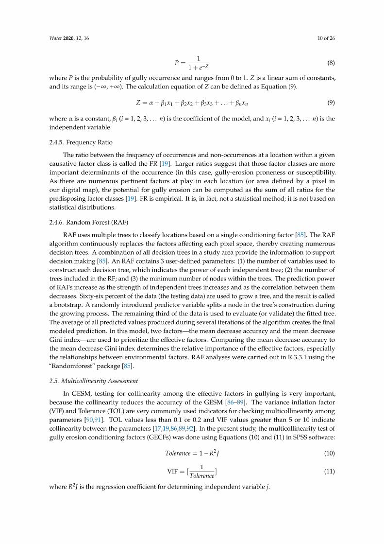
Gully erosion susceptibility mapping using four machine-learning models provided four predictions of gully formation zones (Table 3 and Figure 7a–d). According to all four models used in the study, most of the study area is classified as having very low and low susceptibility to gully erosion (ADTree—55.2% (1201.1 km2), Bagging-ADTree—53.38% (1161.4 km2), RF-ADTree—52.81% (1149.1 km2), and LR—47.25% (1028.1 km2)). ADTree classified the largest total area of very low susceptibility (36.30%) and the smallest total area of very high susceptibility (4.63%). The other models classified 30.43% (Bad-ADTree), 22.69% (RF-ADTree), and 22.07% (LR) as very low susceptibility, and 8.86% (Bad-ADTree), 10.34% (RF-ADTree), and 12.66% (LR) as having very high susceptibility. Among the models, LR classified the largest portion of the study area as highly susceptible (12.66%) and the smallest portion as having very low susceptibility (22.07%).

Figure 6. Relative importance of conditioning factors using a random forest model.

3.4. Gully Erosion Susceptibility Mapping Using Machine Learning Models

Gully erosion susceptibility mapping using four machine-learning models provided fourpredictions of gully formation zones (Table 3 and Figure 7a–d). According to all four modelsused in the study, most of the study area is classified as having very low and low susceptibility to gullyerosion (ADTree—55.2% (1201.1 km2), Bagging-ADTree—53.38% (1161.4 km2), RF-ADTree—52.81%(1149.1 km2), and LR—47.25% (1028.1 km2)). ADTree classified the largest total area of very lowsusceptibility (36.30%) and the smallest total area of very high susceptibility (4.63%). The other modelsclassified 30.43% (Bad-ADTree), 22.69% (RF-ADTree), and 22.07% (LR) as very low susceptibility, and8.86% (Bad-ADTree), 10.34% (RF-ADTree), and 12.66% (LR) as having very high susceptibility. Amongthe models, LR classified the largest portion of the study area as highly susceptible (12.66%) and thesmallest portion as having very low susceptibility (22.07%).

Water 2020, 12, 16 16 of 26

Water 2020, 12, x FOR PEER REVIEW 15 of 26

3.3. The Relative Importance of GECFs

RAF modeling revealed the importance of GECFs (Figure 6). Distance-to-road (16.95) was the most important factor in gully occurrence in the study area. The other factors, in the order of importance were drainage density (14), distance-to-stream (13.29), LU/LC (10.58), annual rainfall (9.1), TWI (6.91), NDVI (6.6), elevation (6), SPI (5.2), TPI (4.67), CI (2.87), lithology (2.76), soil type (2.57), slope (1.4), plan curvature (1.4), TRI (0.75), aspect (0.18), and LS (0.034).

Figure 6. Relative importance of conditioning factors using a random forest model.

3.4. Gully Erosion Susceptibility Mapping Using Machine Learning Models

Gully erosion susceptibility mapping using four machine-learning models provided four predictions of gully formation zones (Table 3 and Figure 7a–d). According to all four models used in the study, most of the study area is classified as having very low and low susceptibility to gully erosion (ADTree—55.2% (1201.1 km2), Bagging-ADTree—53.38% (1161.4 km2), RF-ADTree—52.81% (1149.1 km2), and LR—47.25% (1028.1 km2)). ADTree classified the largest total area of very low susceptibility (36.30%) and the smallest total area of very high susceptibility (4.63%). The other models classified 30.43% (Bad-ADTree), 22.69% (RF-ADTree), and 22.07% (LR) as very low susceptibility, and 8.86% (Bad-ADTree), 10.34% (RF-ADTree), and 12.66% (LR) as having very high susceptibility. Among the models, LR classified the largest portion of the study area as highly susceptible (12.66%) and the smallest portion as having very low susceptibility (22.07%).

Water 2020, 12, x FOR PEER REVIEW 16 of 26

Figure 7. Gully erosion susceptibility map using (a) Alternating decision tree (ADTree), (b) Rotation Forest (RF)-ADTree, (c) Bagging-ADTree, (d) Logistic regression.

3.5. Validation of Results

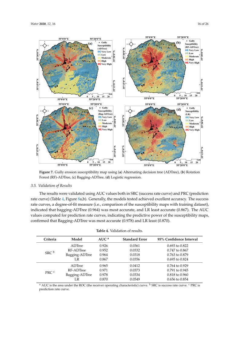
The results were validated using AUC values both in SRC (success rate curve) and PRC (prediction rate curve) (Table 4, Figure 8a,b). Generally, the models tested achieved excellent accuracy. The success rate curves, a degree-of-fit measure (i.e., comparison of the susceptibility maps with training dataset), indicated that bagging-ADTree (0.964) was most accurate, and LR least accurate (0.867). The AUC values computed for prediction rate curves, indicating the predictive power of the susceptibility maps, confirmed that Bagging-ADTree was most accurate (0.978) and LR least (0.870).

Figure 8. Validation of results using (a) area under the curve of success rate curve and (b) prediction rate curve.

Figure 7. Gully erosion susceptibility map using (a) Alternating decision tree (ADTree), (b) RotationForest (RF)-ADTree, (c) Bagging-ADTree, (d) Logistic regression.

3.5. Validation of Results

The results were validated using AUC values both in SRC (success rate curve) and PRC (predictionrate curve) (Table 4, Figure 8a,b). Generally, the models tested achieved excellent accuracy. The successrate curves, a degree-of-fit measure (i.e., comparison of the susceptibility maps with training dataset),indicated that bagging-ADTree (0.964) was most accurate, and LR least accurate (0.867). The AUCvalues computed for prediction rate curves, indicating the predictive power of the susceptibility maps,confirmed that Bagging-ADTree was most accurate (0.978) and LR least (0.870).

Table 4. Validation of results.

Criteria Model AUC a Standard Error 95% Confidence Interval

SRC b

ADTree 0.926 0.0361 0.693 to 0.822RF-ADTree 0.952 0.0332 0.747 to 0.867

Bagging-ADTree 0.964 0.0318 0.763 to 0.879LR 0.867 0.0356 0.695 to 0.824

PRC c

ADTree 0.965 0.0412 0.764 to 0.929RF-ADTree 0.971 0.0373 0.791 to 0.945

Bagging-ADTree 0.978 0.0334 0.818 to 0.960LR 0.870 0.0549 0.656 to 0.854

a AUC is the area under the ROC (the receiver operating characteristic) curve. b SRC is success rate curve. c PRC isprediction rate curve.

Water 2020, 12, 16 17 of 26

Water 2020, 12, x FOR PEER REVIEW 16 of 26

Figure 7. Gully erosion susceptibility map using (a) Alternating decision tree (ADTree), (b) Rotation Forest (RF)-ADTree, (c) Bagging-ADTree, (d) Logistic regression.

3.5. Validation of Results

The results were validated using AUC values both in SRC (success rate curve) and PRC (prediction rate curve) (Table 4, Figure 8a,b). Generally, the models tested achieved excellent accuracy. The success rate curves, a degree-of-fit measure (i.e., comparison of the susceptibility maps with training dataset), indicated that bagging-ADTree (0.964) was most accurate, and LR least accurate (0.867). The AUC values computed for prediction rate curves, indicating the predictive power of the susceptibility maps, confirmed that Bagging-ADTree was most accurate (0.978) and LR least (0.870).

Figure 8. Validation of results using (a) area under the curve of success rate curve and (b) prediction rate curve.

Figure 8. Validation of results using (a) area under the curve of success rate curve and (b) predictionrate curve.

4. Discussion

Different sources were used to prepare the input dataset. Because many factors used in GESMwere extracted from a digital elevation model (DEM), the quality of the DEM significantly influencesthe accuracy of the results [96,97]. The Advanced Land Observing Satellite (ALOS) DEM with 12.5 mspatial resolution was used as it has been shown to provide better accuracy than both the Shuttle RadarTopography Mission (SRTM) and Advanced Spaceborne Thermal Emission and Reflection Radiometer(ASTER) and DEMs [98].

In this study, we developed and explored a new ensemble intelligence approach using bagging andRF as a meta-classifier and with ADTree as a base classifier, to spatially predict gully head-cut erosionin the Chah Mousi watershed. We produced GESMs based on a modeling procedure including trainingand validation datasets, and 18 conditioning factors (elevation, slope angle, aspect, plan curvature, CI,LS, SPI, TPI, TRI, TWI, distance to stream, drainage density, rainfall, distance to road, NDVI, lithology,land use/land cover, and soil type). These factors were checked for collinearity with statistical metrics,including TOL and VIF. The results reveal that all GECFs influenced gully erosion occurrence.

Based on FR analysis, the relationship between the factors and gully locations wereassessed. Conditioning-factor classes with FR values >1 indicated areas with greater gully-erosionsusceptibility [82]. Elevation plays an important role in vegetation and precipitation type and, therefore,controls the spatial distribution and gully erosion processes [99]. Elevations in the study region below1000 m a.s.l. are more susceptible to gully erosion. Thus, the higher occurrence of gully head cuterosion in the lowland areas agrees with Dickson et al. [100]. However, Arabamiri et al. [19] determinedthat elevations below 829 m were most prone to gullying. In terms of slope angle and curvature, theFR analysis showed that slopes of less than 5◦ (including flat areas) were most likely to be sites ofgully occurrence. Because lower slope angles have greater soil depth, intensive rainfall impaction andgreater runoff from upslope will decrease soil strength resulting in the development and extension ofthe gully channel [9]. Curvature causes accumulation of runoff and enhances the velocity and volumeof flow, so this variable positively correlates to locations of gully erosion. The slope aspect that controlsseveral climate conditions, such as the intensity of precipitation, moisture, evapotranspiration, andvegetation cover [101], indirectly influences gully erosion. Among the slope-aspect classes, east- andsoutheast-facing slopes are the most highly correlated to gully erosion. These two slope aspect classesget more solar radiation in the northern hemisphere and, as a result, they experience more evaporation,higher soil porosity (total pore space), lower soil strength, and lower vegetation density. This is inaccordance with Zabihi et al. [9], who reported that southward slope aspects are more susceptible

Water 2020, 12, 16 18 of 26

to gully erosion. CI values below −39.6 100/m were most predictive of gully formation: the lowerthe CI value, the greater is the potential for gully erosion. Arabameri et al. [17] concluded, based onthe WoE method, that CI values between 0 and 10 signify locations that are more susceptible to gullyoccurrence in their study area. LS less than 15 m indicate a more likely formation of gullies and reflectsthat gullies are more likely formed in flat areas with lower slope angles. This confirms the findings ofGayen et al. [102], but conflicts with the results of Zabihi et al. [9], who shows a direct relationshipbetween LS and gully erosion locations. Zabihi et al. also implied that the higher the LS, the higher theprobability of gully erosion occurrence due to increasing runoff velocity and a decreasing detachmentand transport threshold of soil particles [103,104].

The most susceptible classes for the other GECFs were SPI between >14.9, TPI less than−7, TRI lessthan 1.4, and TWI more than 11.8. These results are confirmed by the findings of Arabameri et al. [17]who reported that, for example, the greater the TWI factor, the greater is the potential for gullyoccurrence. High values of TWI increase the filtration rate and provide the conditions for piping androof collapse, resulting in the development of gully tunnels and, eventually, the appearance of gullieson the surface [105].

Moreover, the nearer sites are to a river, the higher the susceptibility to gully erosion. In thisstudy, locations at distances less than 100 m from a stream were more likely to see gully formation.Some researchers have confirmed these results [9,13,16,42]. The sheer force of flow can overcome anddecrease the strength of soil along the sides of gully forms and lead to the development of gullies ofgreater dimensions.

Areas with drainage densities exceeding 1.75 km/km2 were most correlated to gully erosion.The role of this factor can be made clearer when other factors are considered. For example, a locationwith a lower slope angle and higher drainage density has a higher TWI, and if the soil at that locationwas loose and erodible, gully erosion is easier to achieve. In the study area, the lower classes of annualprecipitation amounts (between 68.3 and 85.7 mm) were most susceptible to gully incidence. Thissuggests that though rainfall has a positive role in gully formation, it is not the most important factor.In other words, lower rainfall values are positively related to gullying.

Distances from roads are important to gully erosion and, like distances from rivers, the nearerthe site, the higher the potential for gully erosion. Distances of less than 500 m from a road werepositively correlated to gully locations, which underscores the importance of the roles of developmentand disturbance of ground surfaces in promoting landscape degradation.

Results of the NDVI factor show that vegetation plays a very important role in protecting soilagainst erosion, so that, with increasing vegetation, the sensitivity of an area to gully erosion decreases.Vegetation cover greatly reduces the erosion of runoff through the increase in infiltration and protectionof soil through roots [106]. The findings agree with those of Arabameri et al. [13], Arabameri et al. [19],and Chaplot et al. [107] stating that low values of NDVI have a positive association with gully erosionand that it is easier for a gully to develop in areas with lower NDVI values. Generally, barren lands andsparsely vegetated areas are more susceptible to erosion than forests, where vegetation cover stronglyreduces the erosive action of surface runoff.

Because gully erosion depends on the lithological properties of materials at Earth’s surface,lithology is a vital factor in gullying [104]. As for lithology, Quaternary lithotypes have a highsusceptibility to gully erosion. The result is in agreement with findings reported by Arabameri et al. [13],who found that Quaternary lithotypes have a strong effect on gully occurrences. In terms of land use,which plays a key role in geomorphological and hydrological processes by controlling overland flowrunoff generation and sediment dynamics [108], the areas of kavir are most susceptible to gully erosion.In these regions, the complete lack of vegetation leaves the soil exposed, and it is easily eroded byprecipitation. These results are in line with [13]. The entisol/aridisol soils are the most susceptible soilsto gully erosion occurring in the study area, which is in accordance with [19].

In terms of the FR values, the most important GECFs in the study area were the distance tonearest road and drainage density. This is confirmed by the RAF algorithm analysis, which was used

Water 2020, 12, 16 19 of 26

to rank the importance of the GECFs for the spatial prediction of gullies in the study area. This resultis consistent with [17,109,110]. Roads are impervious surfaces, and they disrupt natural drainagesystems due to improper culverts, concentration of surface runoffs, and by altering the hydrologicalfunctions of hillslopes, which significantly contribute to overland flow and allow rapid run-off, easilyeroding bare soil and causing gullying [111,112]. An example of the effect of roads on gullying isshown in Figure 9. Distance to a road is the most important factor. It is followed in importance bydrainage density, distance to stream, land use, rainfall, NDVI, elevation, SPI, TPI, CI, lithology, soiltype, plan curvature, TRI, aspect, and LS. Though other factors affect gully erosion, the above are themost meaningful in the study area.

Water 2020, 12, x FOR PEER REVIEW 19 of 26

drainage density, distance to stream, land use, rainfall, NDVI, elevation, SPI, TPI, CI, lithology, soil type, plan curvature, TRI, aspect, and LS. Though other factors affect gully erosion, the above are the most meaningful in the study area.

A novel ensemble intelligence approach, bagging-ADTree, and other ML algorithms—ADTree, RF-ADTree and LR—were used to create gully erosion susceptibility maps. The goodness-of-fit and the performance of the models were checked by AUROC of success and prediction rate curves. The results illustrate that bagging ADTree and RF-ADTree outperformed ADTree and LR. These results are in line with [42,113,114]. The new model accurately identified the areas that are susceptible to gully erosion based on the past patterns of formation, but it also provides excellent predictions of future development. The RF and bagging as a meta-classifier can decrease over-fitting and noise problems in the training dataset. Some researchers have confirmed the prediction power of RF in applications to some environmental problems [42,115–117].

For example, Tien Bui et al. [21] predicted gully locations in a semi-arid watershed of Iran using ADTtree and its ensembles using RF meta-classifier. They concluded that the RF model could well enhance the prediction power of ADTree as a base classifier. However, the RF-ADTree ensemble model outperformed some benchmark models, including SVM based on the polynomial and RBF kernels, LR, naïve Bayes, and ADTtree. Additionally, Shirzadi et al. [42] used four meta-classifiers, namely, multiboost, bagging, RF, and random subspace (RS), for the spatial prediction of shallow landslides in Bijar City, Kurdistan province, Iran. They used ADTree as a base classifier for the modeling process. The four ensemble models were combined with the ADTree under two scenarios of different sample sizes and raster resolutions. They reported that the RS model was more capable for sample sizes of 60%/40% and 70%/30% with a raster resolution of 10 m. According to the results, the new proposed ensemble model can spatially predict gully erosion occurrences with reasonably good accuracy.

Figure 9. A sample of road effect on gully occurrence.

5. Conclusions

Soil erosion is an important environmental challenge to ecosystem’s condition and function. Land degradation and decreasing land productivity are a result of on-site and off-site erosion in a gully-prone area. However, detection, prediction, and management of gully-prone areas using protective measures and mitigation techniques are important efforts. Some quantitative and qualitative methods and techniques have been developed and explored for modeling and preparing

Figure 9. A sample of road effect on gully occurrence.

A novel ensemble intelligence approach, bagging-ADTree, and other ML algorithms—ADTree,RF-ADTree and LR—were used to create gully erosion susceptibility maps. The goodness-of-fit and theperformance of the models were checked by AUROC of success and prediction rate curves. The resultsillustrate that bagging ADTree and RF-ADTree outperformed ADTree and LR. These results are inline with [42,113,114]. The new model accurately identified the areas that are susceptible to gullyerosion based on the past patterns of formation, but it also provides excellent predictions of futuredevelopment. The RF and bagging as a meta-classifier can decrease over-fitting and noise problems inthe training dataset. Some researchers have confirmed the prediction power of RF in applications tosome environmental problems [42,115–117].

For example, Tien Bui et al. [21] predicted gully locations in a semi-arid watershed of Iran usingADTtree and its ensembles using RF meta-classifier. They concluded that the RF model could wellenhance the prediction power of ADTree as a base classifier. However, the RF-ADTree ensemble modeloutperformed some benchmark models, including SVM based on the polynomial and RBF kernels,LR, naïve Bayes, and ADTtree. Additionally, Shirzadi et al. [42] used four meta-classifiers, namely,multiboost, bagging, RF, and random subspace (RS), for the spatial prediction of shallow landslides inBijar City, Kurdistan province, Iran. They used ADTree as a base classifier for the modeling process.The four ensemble models were combined with the ADTree under two scenarios of different samplesizes and raster resolutions. They reported that the RS model was more capable for sample sizes of

Water 2020, 12, 16 20 of 26

60%/40% and 70%/30% with a raster resolution of 10 m. According to the results, the new proposedensemble model can spatially predict gully erosion occurrences with reasonably good accuracy.

5. Conclusions

Soil erosion is an important environmental challenge to ecosystem’s condition and function.Land degradation and decreasing land productivity are a result of on-site and off-site erosionin a gully-prone area. However, detection, prediction, and management of gully-prone areasusing protective measures and mitigation techniques are important efforts. Some quantitative andqualitative methods and techniques have been developed and explored for modeling and preparingthe susceptibility assessments. However, due to differences in their probability distribution functions,their performances are also different. For example, some of them do not fit the data that are available.All models present advantages and disadvantages, so one of the most important aspects of themodeling strategy is selecting the appropriate model. Machine-learning models are more often usedbecause of their ability to overcome over-fitting and noise challenges during the modeling process andbecause they have higher goodness-of-fits and perform better compared to other conventional models.Moreover, among the machine-learning classifiers, ensemble models are more powerful than singleclassifiers. They randomly divide a training dataset into subsets and perform a single classifier, whichprovides an output with the lowest error and the highest performance rather than the single classifier.This process overcomes the weakness of the single classifier and achieves a more powerful classifier.In response to the advantage of ensemble classifiers, a novel ensemble intelligence approach, namelybagging-ADTree, was performed and gully erosion maps were obtained. Some other machine-learningalgorithms (including ADTree, Bagging-ADTree, and LR) were used for comparison and validation ofthe results of the new model. The random forest model is used to determine the relative importance ofconditioning factors. The results indicate that distance-to-road and drainage density are very importantto gully occurrence in the study area. The validation indicated that although the models achieved highgoodness-of-fit scores and were powerfully predictive, the ensemble model was better than othersat spatially predicting gully erosion and produced a more accurate gully-susceptibility map of thestudy area. Based on these results, we can recommend the new model, bagging-ADTree, for gullymodeling in other zones of potential gully erosion susceptibility, but offer one caution: there may beother conditioning factors responsible for gully erosion in other areas. Finally, the results from a casestudy of the Chah Mousi watershed show that selecting suitable predisposing factors and combiningmachine-learning ensemble models with GISs can be used to efficiently predict an area’s susceptibilityto gully formation with high accuracy. Therefore, the gully-erosion susceptibility map generated bythe method can aid decision makers, planners, and engineers in their quests to identify and developthe most effective protective measures to sustainably prevent and mitigate gully-erosion damage.

Author Contributions: Conceptualization, A.A.; data curation, A.A.; formal analysis, A.A. and W.C.; investigation,A.A. and D.T.B.; methodology, A.A., W.C., B.P., and D.T.B.; resources, A.A., software, A.A. and W.C.; supervision,A.A.; validation, A.A.; writing—original draft, A.A.; writing—review and editing, A.A., W.C., T.B., B.P., J.P.T., andD.T.B. All authors have read and agreed to the published version of the manuscript.

Funding: This research was partly funded by the Austrian Science Fund (FWF) through the Doctoral CollegeGIScience (DK W 1237-N23) at the University of Salzburg.

Conflicts of Interest: The authors declare no conflict of interest.

References

1. Poesen, J.; Nachtergaele, J.; Verstraeten, G.; Valentin, C. Gully erosion and environmental change: Importanceand research needs. Catena 2003, 50, 91–133. [CrossRef]

2. Valentin, C.; Poesen, J.; Li, Y. Gully erosion: Impacts, factors and control. Catena 2005, 63, 132–153. [CrossRef]3. Kirkby, M.; Bracken, L. Gully processes and gully dynamics. Earth Surf. Process. Landf. J. Br. Geomorphol. Res.

Group 2009, 34, 1841–1851. [CrossRef]

Water 2020, 12, 16 21 of 26

4. Poesen, J.; Vanwalleghem, T.; Deckers, J. Gullies and Closed Depressions in the Loess Belt: Scars ofHuman–Environment Interactions. In Landscapes and Landforms of Belgium and Luxembourg; Springer:Berlin/Heidelberg, Germany, 2018; pp. 253–267.

5. Pandey, A.; Chowdary, V.; Mal, B. Identification of critical erosion prone areas in the small agriculturalwatershed using USLE, GIS and remote sensing. Water Resour. Manag. 2007, 21, 729–746. [CrossRef]

6. Martınez-Casasnovas, J. A spatial information technology approach for the mapping and quantification ofgully erosion. Catena 2003, 50, 293–308. [CrossRef]

7. Zinck, J.A.; López, J.; Metternicht, G.I.; Shrestha, D.P.; Vázquez-Selem, L. Mapping and modelling massmovements and gullies in mountainous areas using remote sensing and GIS techniques. Int. J. Appl. EarthObs. Geoinf. 2001, 3, 43–53. [CrossRef]

8. Seutloali, K.E.; Beckedahl, H.R.; Dube, T.; Sibanda, M. An assessment of gully erosion along major armouredroads in south-eastern region of South Africa: A remote sensing and GIS approach. Geocarto Int. 2016, 31,225–239. [CrossRef]

9. Zabihi, M.; Mirchooli, F.; Motevalli, A.; Darvishan, A.K.; Pourghasemi, H.R.; Zakeri, M.A.; Sadighi, F. Spatialmodelling of gully erosion in Mazandaran Province, northern Iran. Catena 2018, 161, 1–13. [CrossRef]

10. Conoscenti, C.; Angileri, S.; Cappadonia, C.; Rotigliano, E.; Agnesi, V.; Märker, M. Gully erosion susceptibilityassessment by means of GIS-based logistic regression: A case of Sicily (Italy). Geomorphology 2014, 204,399–411. [CrossRef]

11. Vanwalleghem, T.; Van Den Eeckhaut, M.; Poesen, J.; Govers, G.; Deckers, J. Spatial analysis of factorscontrolling the presence of closed depressions and gullies under forest: Application of rare event logisticregression. Geomorphology 2008, 95, 504–517. [CrossRef]

12. Rahmati, O.; Haghizadeh, A.; Pourghasemi, H.R.; Noormohamadi, F. Gully erosion susceptibility mapping:The role of GIS-based bivariate statistical models and their comparison. Nat. Hazards 2016, 82, 1231–1258.[CrossRef]

13. Arabameri, A.; Pradhan, B.; Pourghasemi, H.; Rezaei, K.; Kerle, N. Spatial modelling of gully erosion usingGIS and R programing: A comparison among three data mining algorithms. Appl. Sci. 2018, 8, 1369.[CrossRef]

14. Magliulo, P. Soil erosion susceptibility maps of the Janare Torrent Basin (southern Italy). J. Maps 2010, 6,435–447. [CrossRef]

15. Conoscenti, C.; Agnesi, V.; Angileri, S.; Cappadonia, C.; Rotigliano, E.; Märker, M. A GIS-based approachfor gully erosion susceptibility modelling: A test in Sicily, Italy. Environ. Earth Sci. 2013, 70, 1179–1195.[CrossRef]

16. Arabameri, A.; Pradhan, B.; Rezaei, K.; Lee, C.-W. Assessment of Landslide Susceptibility Using Statistical-andArtificial Intelligence-Based FR–RF Integrated Model and Multiresolution DEMs. Remote Sens. 2019, 11, 999.[CrossRef]

17. Arabameri, A.; Rezaei, K.; Pourghasemi, H.R.; Lee, S.; Yamani, M. GIS-based gully erosion susceptibilitymapping: A comparison among three data-driven models and AHP knowledge-based technique. Environ.Earth Sci. 2018, 77, 628. [CrossRef]

18. Svoray, T.; Michailov, E.; Cohen, A.; Rokah, L.; Sturm, A. Predicting gully initiation: Comparing data miningtechniques, analytical hierarchy processes and the topographic threshold. Earth Surf. Process. Landf. 2012, 37,607–619. [CrossRef]

19. Arabameri, A.; Pradhan, B.; Rezaei, K.; Conoscenti, C. Gully erosion susceptibility mapping using GIS-basedmulti-criteria decision analysis techniques. Catena 2019, 180, 282–297. [CrossRef]

20. Amiri, M.; Pourghasemi, H.R.; Ghanbarian, G.A.; Afzali, S.F. Assessment of the importance of gully erosioneffective factors using Boruta algorithm and its spatial modeling and mapping using three machine learningalgorithms. Geoderma 2019, 340, 55–69. [CrossRef]

21. Tien Bui, D.; Shirzadi, A.; Shahabi, H.; Chapi, K.; Omidavr, E.; Pham, B.T.; Talebpour Asl, D.; Khaledian, H.;Pradhan, B.; Panahi, M. A Novel Ensemble Artificial Intelligence Approach for Gully Erosion Mapping in aSemi-Arid Watershed (Iran). Sensors 2019, 19, 2444. [CrossRef]

22. Jaafari, A.; Zenner, E.K.; Panahi, M.; Shahabi, H. Hybrid artificial intelligence models based on a neuro-fuzzysystem and metaheuristic optimization algorithms for spatial prediction of wildfire probability. Agric. For.Meteorol. 2019, 266, 198–207. [CrossRef]

Water 2020, 12, 16 22 of 26

23. Taheri, K.; Shahabi, H.; Chapi, K.; Shirzadi, A.; Gutiérrez, F.; Khosravi, K. Sinkhole susceptibility mapping:A comparison between Bayes-based machine learning algorithms. Land Degrad. Dev. 2019, 30, 730–745.[CrossRef]

24. Chapi, K.; Singh, V.P.; Shirzadi, A.; Shahabi, H.; Bui, D.T.; Pham, B.T.; Khosravi, K. A novel hybrid artificialintelligence approach for flood susceptibility assessment. Environ. Model. Softw. 2017, 95, 229–245. [CrossRef]

25. Hong, H.; Panahi, M.; Shirzadi, A.; Ma, T.; Liu, J.; Zhu, A.-X.; Chen, W.; Kougias, I.; Kazakis, N. Floodsusceptibility assessment in Hengfeng area coupling adaptive neuro-fuzzy inference system with geneticalgorithm and differential evolution. Sci. Total Environ. 2018, 621, 1124–1141. [CrossRef] [PubMed]

26. Khosravi, K.; Pham, B.T.; Chapi, K.; Shirzadi, A.; Shahabi, H.; Revhaug, I.; Prakash, I.; Bui, D.T. A comparativeassessment of decision trees algorithms for flash flood susceptibility modeling at Haraz watershed, northernIran. Sci. Total Environ. 2018, 627, 744–755. [CrossRef] [PubMed]

27. Shafizadeh-Moghadam, H.; Valavi, R.; Shahabi, H.; Chapi, K.; Shirzadi, A. Novel forecasting approachesusing combination of machine learning and statistical models for flood susceptibility mapping. J. Environ.Manag. 2018, 217, 1–11. [CrossRef]

28. Ahmadlou, M.; Karimi, M.; Alizadeh, S.; Shirzadi, A.; Parvinnejhad, D.; Shahabi, H.; Panahi, M. Floodsusceptibility assessment using integration of adaptive network-based fuzzy inference system (ANFIS) andbiogeography-based optimization (BBO) and BAT algorithms (BA). Geocarto Int. 2018, 34, 1–21. [CrossRef]

29. Bui, D.T.; Panahi, M.; Shahabi, H.; Singh, V.P.; Shirzadi, A.; Chapi, K.; Khosravi, K.; Chen, W.; Panahi, S.; Li, S.Novel hybrid evolutionary algorithms for spatial prediction of floods. Sci. Rep. 2018, 8, 15364. [CrossRef]

30. Miraki, S.; Zanganeh, S.H.; Chapi, K.; Singh, V.P.; Shirzadi, A.; Shahabi, H.; Pham, B.T. Mapping GroundwaterPotential Using a Novel Hybrid Intelligence Approach. Water Resour. Manag. 2019, 33, 281–302. [CrossRef]

31. Rahmati, O.; Naghibi, S.A.; Shahabi, H.; Bui, D.T.; Pradhan, B.; Azareh, A.; Rafiei-Sardooi, E.; Samani, A.N.;Melesse, A.M. Groundwater spring potential modelling: Comprising the capability and robustness of threedifferent modeling approaches. J. Hydrol. 2018, 565, 248–261. [CrossRef]

32. Tien Bui, D.; Khosravi, K.; Li, S.; Shahabi, H.; Panahi, M.; Singh, V.; Chapi, K.; Shirzadi, A.; Panahi, S.;Chen, W. New hybrids of anfis with several optimization algorithms for flood susceptibility modeling. Water2018, 10, 1210. [CrossRef]

33. Tehrany, M.S.; Pradhan, B.; Jebur, M.N. Flood susceptibility analysis and its verification using a novelensemble support vector machine and frequency ratio method. Stoch. Environ. Res. Risk Assess. 2015, 29,1149–1165. [CrossRef]

34. Rahmati, O.; Samadi, M.; Shahabi, H.; Azareh, A.; Rafiei-Sardooi, E.; Alilou, H.; Melesse, A.M.; Pradhan, B.;Chapi, K.; Shirzadi, A. SWPT: An automated GIS-based tool for prioritization of sub-watersheds based onmorphometric and topo-hydrological factors. Geosci. Front. 2019, 10, 2167–2175. [CrossRef]

35. Khosravi, K.; Shahabi, H.; Pham, B.T.; Adamawoski, J.; Shirzadi, A.; Pradhan, B.; Dou, J.; Ly, H.-B.;Gróf, G.; Ho, H.L.; et al. A Comparative Assessment of Flood Susceptibility Modeling Using Multi-CriteriaDecision-Making Analysis and Machine Learning Methods. J. Hydrol. 2019, 573, 311–323. [CrossRef]

36. Chen, W.; Panahi, M.; Khosravi, K.; Pourghasemi, H.R.; Rezaie, F.; Parvinnezhad, D. Spatial prediction ofgroundwater potentiality using anfis ensembled with teaching-learning-based and biogeography-basedoptimization. J. Hydrol. 2019, 572, 435–448. [CrossRef]

37. Chen, W.; Pradhan, B.; Li, S.; Shahabi, H.; Rizeei, H.M.; Hou, E.; Wang, S. Novel hybrid integration approachof bagging-based fisher’s linear discriminant function for groundwater potential analysis. Nat. Resour. Res.2019, 28, 1239–1258. [CrossRef]

38. Chen, W.; Tsangaratos, P.; Ilia, I.; Duan, Z.; Chen, X. Groundwater spring potential mapping usingpopulation-based evolutionary algorithms and data mining methods. Sci. Total Environ. 2019, 684, 31–49.[CrossRef]

39. Roodposhti, M.S.; Safarrad, T.; Shahabi, H. Drought sensitivity mapping using two one-class support vectormachine algorithms. Atmos. Res. 2017, 193, 73–82. [CrossRef]

40. Alizadeh, M.; Alizadeh, E.; Asadollahpour Kotenaee, S.; Shahabi, H.; Beiranvand Pour, A.; Panahi, M.;Bin Ahmad, B.; Saro, L. Social vulnerability assessment using artificial neural network (ANN) model forearthquake hazard in Tabriz city, Iran. Sustainability 2018, 10, 3376. [CrossRef]

41. Tien Bui, D.; Shahabi, H.; Shirzadi, A.; Chapi, K.; Pradhan, B.; Chen, W.; Khosravi, K.; Panahi, M.; BinAhmad, B.; Saro, L. Land subsidence susceptibility mapping in south korea using machine learning algorithms.Sensors 2018, 18, 2464. [CrossRef]

Water 2020, 12, 16 23 of 26

42. Shirzadi, A.; Soliamani, K.; Habibnejhad, M.; Kavian, A.; Chapi, K.; Shahabi, H.; Chen, W.; Khosravi, K.; ThaiPham, B.; Pradhan, B. Novel GIS based machine learning algorithms for shallow landslide susceptibilitymapping. Sensors 2018, 18, 3777. [CrossRef] [PubMed]

43. Pham, B.T.; Prakash, I.; Singh, S.K.; Shirzadi, A.; Shahabi, H.; Bui, D.T. Landslide susceptibility modelingusing Reduced Error Pruning Trees and different ensemble techniques: Hybrid machine learning approaches.CATENA 2019, 175, 203–218. [CrossRef]

44. Tien Bui, D.; Shahabi, H.; Shirzadi, A.; Kamran Chapi, K.; Hoang, N.-D.; Pham, B.; Bui, Q.-T.; Tran, C.-T.;Panahi, M.; Bin Ahmad, B.; et al. A Novel Integrated Approach of Relevance Vector Machine Optimized byImperialist Competitive Algorithm for Spatial Modeling of Shallow Landslides. Remote Sens. 2019, 11, 57.[CrossRef]

45. Thai Pham, B.; Prakash, I.; Dou, J.; Singh, S.K.; Trinh, P.T.; Trung Tran, H.; Minh Le, T.; Tran, V.P.; KimKhoi, D.; Shirzadi, A. A Novel Hybrid Approach of Landslide Susceptibility Modeling Using Rotation ForestEnsemble and Different Base Classifiers. Geocarto Int. 2018. [CrossRef]

46. Chen, W.; Shahabi, H.; Zhang, S.; Khosravi, K.; Shirzadi, A.; Chapi, K.; Pham, B.T.; Zhang, T.; Zhang, L.;Chai, H.; et al. Landslide susceptibility modeling based on gis and novel bagging-based kernel logisticregression. Appl. Sci. 2018, 8, 2540. [CrossRef]

47. Chen, W.; Hong, H.; Panahi, M.; Shahabi, H.; Wang, Y.; Shirzadi, A.; Pirasteh, S.; Alesheikh, A.A.; Khosravi, K.;Panahi, S.; et al. Spatial prediction of landslide susceptibility using gis-based data mining techniques of anfiswith whale optimization algorithm (woa) and grey wolf optimizer (gwo). Appl. Sci. 2019, 9, 3755. [CrossRef]

48. Chen, W.; Pourghasemi, H.R.; Naghibi, S.A. Prioritization of landslide conditioning factors and its spatialmodeling in shangnan county, china using gis-based data mining algorithms. Bull. Eng. Geol. Environ. 2018,77, 611–629. [CrossRef]

49. Kuhnert, P.M.; Henderson, A.K.; Bartley, R.; Herr, A. Incorporating uncertainty in gully erosion calculationsusing the random forests modelling approach. Environmetrics 2010, 21, 493–509. [CrossRef]

50. Shruthi, R.B.; Kerle, N.; Jetten, V.; Stein, A. Object-based gully system prediction from medium resolutionimagery using Random Forests. Geomorphology 2014, 216, 283–294. [CrossRef]

51. Rahmati, O.; Tahmasebipour, N.; Haghizadeh, A.; Pourghasemi, H.R.; Feizizadeh, B. Evaluation of differentmachine learning models for predicting and mapping the susceptibility of gully erosion. Geomorphology 2017,298, 118–137. [CrossRef]

52. Pourghasemi, H.R.; Yousefi, S.; Kornejady, A.; Cerdà, A. Performance assessment of individual and ensembledata-mining techniques for gully erosion modeling. Sci. Total Environ. 2017, 609, 764–775. [CrossRef][PubMed]

53. Yunkai, L.; Yingjie, T.; Zhiyun, O.; Lingyan, W.; Tingwu, X.; Peiling, Y.; Huanxun, Z. Analysis of soil erosioncharacteristics in small watersheds with particle swarm optimization, support vector machine, and artificialneuronal networks. Environ. Earth Sci. 2010, 60, 1559–1568. [CrossRef]

54. Gutiérrez, Á.G.; Schnabel, S.; Contador, J.F.L. Using and comparing two nonparametric methods (CART andMARS) to model the potential distribution of gullies. Ecol. Model. 2009, 220, 3630–3637. [CrossRef]

55. Gutiérrez, Á.G.; Schnabel, S.; Contador, F.L. Gully erosion, land use and topographical thresholds during thelast 60 years in a small rangeland catchment in SW Spain. Land Degrad. Dev. 2009, 20, 535–550. [CrossRef]

56. Angileri, S.E.; Conoscenti, C.; Hochschild, V.; Märker, M.; Rotigliano, E.; Agnesi, V. Water erosion susceptibilitymapping by applying stochastic gradient treeboost to the Imera Meridionale river basin (Sicily, Italy).Geomorphology 2016, 262, 61–76. [CrossRef]

57. Azareh, A.; Rahmati, O.; Rafiei-Sardooi, E.; Sankey, J.B.; Lee, S.; Shahabi, H.; Ahmad, B.B. Modellinggully-erosion susceptibility in a semi-arid region, Iran: Investigation of applicability of certainty factor andmaximum entropy models. Sci. Total Environ. 2019, 655, 684–696. [CrossRef]

58. Conoscenti, C.; Agnesi, V.; Cama, M.; Caraballo-Arias, N.A.; Rotigliano, E. Assessment of gully erosionsusceptibility using multivariate adaptive regression splines and accounting for terrain connectivity.Land Degrad. Dev. 2018, 29, 724–736. [CrossRef]

59. IRIMO. Summary Reports of Iran’s Extreme Climatic Events. In Ministry of Roads and Urban Development;Iran Meteorological Organization: Tehran, Iran, 2012. Available online: http://www.cri.ac.ir (accessed on12 August 2018).

60. GSI. Geology Survey of Iran. 1997. Available online: http://www.gsi.ir/Main/Lang_en/index.html (accessedon 12 August 2018).

Water 2020, 12, 16 24 of 26

61. IUSS Working Group WRB14. World Reference Base for Soil Resources 2014, World Soil Resources Report; FAO:Rome, Italy, 2014.

62. Kuncheva, L.I.; Rodríguez, J.J. An Experimental Study on Rotation Forest Ensembles; Haindl, M., Kittler, J.,Roli, F., Eds.; Springer: Berlin/Heidelberg, Germany, 2007; pp. 459–468.

63. Zhang, C.-X.; Zhang, J.-S. RotBoost: A technique for combining Rotation Forest and AdaBoost. PatternRecognit. Lett. 2008, 29, 1524–1536. [CrossRef]

64. Xia, J.; Du, P.; He, X.; Chanussot, J. Hyperspectral Remote Sensing Image Classification Based on RotationForest. IEEE Geosci. Remote Sens. Lett. 2014, 11, 239–243. [CrossRef]

65. Al-Abadi, A.M. Mapping flood susceptibility in an arid region of southern Iraq using ensemble machinelearning classifiers: A comparative study. Arab. J. Geosci. 2018, 11, 218. [CrossRef]

66. Tien Bui, D.; Shirzadi, A.; Shahabi, H.; Geertsema, M.; Omidvar, E.; Clague, J.J.; Thai Pham, B.; Dou, J.;Talebpour Asl, D.; Bin Ahmad, B.; et al. New Ensemble Models for Shallow Landslide SusceptibilityModeling in a Semi-Arid Watershed. Forests 2019, 10, 743. [CrossRef]

67. Kavzoglu, T.; Colkesen, I. An assessment of the effectiveness of a rotation forest ensemble for land-use andland-cover mapping. Int. J. Remote Sens. 2013, 34, 4224–4241. [CrossRef]

68. Sok, H.K.; Ooi, M.P.-L.; Kuang, Y.C. Sparse alternating decision tree. Pattern Recognit. Lett. 2015, 60–61,57–64. [CrossRef]

69. Hong, H.; Pradhan, B.; Xu, C.; Tien Bui, D. Spatial prediction of landslide hazard at the Yihuang area (China)using two-class kernel logistic regression, alternating decision tree and support vector machines. CATENA2015, 133, 266–281. [CrossRef]

70. Pham, B.T.; Tien Bui, D.; Prakash, I. Landslide Susceptibility Assessment Using Bagging Ensemble BasedAlternating Decision Trees, Logistic Regression and J48 Decision Trees Methods: A Comparative Study.Geotech. Geol. Eng. 2017, 35, 2597–2611. [CrossRef]

71. Freund, Y.; Mason, L. The Alternating Decision Tree Learning Algorithm; Morgan Kaufmann Publishers Inc.:San Francisco, CA, USA, 2002; Volume 99.

72. Dietterich, T.G. An Experimental Comparison of Three Methods for Constructing Ensembles of DecisionTrees: Bagging, Boosting, and Randomization. Mach. Learn. 2000, 40, 139–157. [CrossRef]

73. Breiman, L. Bagging predictors. Mach. Learn. 1996, 24, 123–140. [CrossRef]74. Bryll, R.; Gutierrez-Osuna, R.; Quek, F. Attribute bagging: Improving accuracy of classifier ensembles by

using random feature subsets. Pattern Recognit. 2003, 36, 1291–1302. [CrossRef]75. Buhlmann, P.; Yu, B. Analyzing bagging. Ann. Statist. 2002, 30, 927–961. [CrossRef]76. Pham, B.T.; Tien Bui, D.; Prakash, I. Bagging based Support Vector Machines for spatial prediction of

landslides. Environ. Earth Sci. 2018, 77, 146. [CrossRef]77. Tien Bui, D.; Ho, T.-C.; Pradhan, B.; Pham, B.-T.; Nhu, V.-H.; Revhaug, I. GIS-based modeling of

rainfall-induced landslides using data mining-based functional trees classifier with AdaBoost, Bagging, andMultiBoost ensemble frameworks. Environ. Earth Sci. 2016, 75, 1101. [CrossRef]

78. Truongg, L.X.; Mitamura, M.; Kono, Y.; Raghavan, V.; Yonezawa, G.; Truong, Q.X.; Do, H.T.; Tien Bui, D.;Lee, S. Enhancin Prediction Performance of Landslide Susceptibility Model Using Hybrid Machine LearningApproach of Bagging Ensemble and Logistic Model Tree. Appl. Sci. 2018, 8, 71046.

79. Das, A. Logistic Regression. In Encyclopedia of Quality of Life and Well-Being Research; Michalos, A.C., Ed.;Springer: Dordrecht, The Netherlands, 2014; pp. 3680–3682.

80. Moon, K.-W. Logistic Regression. In Learn ggplot2 Using Shiny App; Moon, K.-W., Ed.; Springer InternationalPublishing: Cham, Switzerland, 2016; pp. 51–54.

81. Raja, N.B.; Çiçek, I.; Türkoglu, N.; Aydin, O.; Kawasaki, A. Correction to: Landslide susceptibility mappingof the Sera River Basin using logistic regression model. Nat. Hazards 2018, 91, 1423. [CrossRef]

82. Meten, M.; Bhandary, N.P.; Yatabe, R. GIS-based frequency ratio and logistic regression modelling forlandslide susceptibility mapping of Debre Sina area in central Ethiopia. J. Mt. Sci. 2015, 12, 1355–1372.[CrossRef]

83. Weisburd, D.; Britt, C. Logistic Regression. In Statistics in Criminal Justice; Weisburd, D., Britt, C., Eds.;Springer: Boston, MA, USA, 2014; pp. 548–600.

84. Pradhan, B. Manifestation of an advanced fuzzy logic model coupled with Geo-information techniques tolandslide susceptibility mapping and their comparison with logistic regression modelling. Environ. Ecol.Stat. 2011, 18, 471–493. [CrossRef]

Water 2020, 12, 16 25 of 26

85. Rodriguez-Galiano, V.; Sanchez-Castillo, M.; Chica-Olmo, M.; Chica-Rivas, M. Machine learning predictivemodels for mineral prospectivity: An evaluation of neural networks, random forest, regression trees andsupport vector machines. Ore Geol. Rev. 2015, 71, 804–818. [CrossRef]

86. Talaei, R. Landslide susceptibility zonation mapping using logistic regression and its validation in HashtchinRegion, northwest of Iran. J. Geol. Soc. India 2014, 84, 68–86. [CrossRef]

87. Arabameri, A.; Cerda, A.; Rodrigo-Comino, J.; Pradhan, B.; Sohrabi, M.; Blaschke, T.; Tien Bui, D. Proposinga Novel Predictive Technique for Gully Erosion Susceptibility Mapping in Arid and Semi-arid Regions (Iran).Remote Sens. 2019, 11, 2577. [CrossRef]

88. Arabameri, A.; Pradhan, B.; Rezaei, K. Spatial prediction of gully erosion using ALOS PALSAR data andensemble bivariate and data mining models. Geosci. J. 2019, 23, 1–18. [CrossRef]

89. Arabameri, A.; Pradhan, B.; Rezaei, K.; Yamani, M.; Pourghasemi, H.R.; Lombardo, L. Spatial modeling ofgully erosion using Evidential Belief Function, Logistic Regression and a new ensemble EBF–LR algorithm.Land Degrad. Dev. 2018, 29, 4035–4049. [CrossRef]

90. Arabameri, A.; Pradhan, B.; Rezaei, K. Gully erosion zonation mapping using integrated geographicallyweighted regression with certainty factor and random forest models in GIS. J. Environ. Manag. 2019, 232,928–942. [CrossRef]

91. Arabameri, A.; Rezaei, K.; Cerdà, A.; Conoscenti, C.; Kalantari, Z. A comparison of statistical methods andmulti-criteria decision making to map flood hazard susceptibility in Northern Iran. Sci. Total Environ. 2019,660, 443–458. [CrossRef] [PubMed]

92. Arabameri, A.; Rezaei, K.; Cerda, A.; Lombardo, L.; Rodrigo-Comino, J. GIS-based groundwater potentialmapping in Shahroud plain, Iran. A comparison among statistical (bivariate and multivariate), data miningand MCDM approaches. Sci. Total Environ. 2019, 658, 160–177. [CrossRef] [PubMed]

93. Chen, W.; Hong, H.; Li, S.; Shahabi, H.; Wang, Y.; Wang, X.; Ahmad, B.B. Flood susceptibility modellingusing novel hybrid approach of reduced-error pruning trees with bagging and random subspace ensembles.J. Hydrol. 2019, 575, 864–873. [CrossRef]

94. Chen, W.; Li, Y.; Xue, W.; Shahabi, H.; Li, S.; Hong, H.; Wang, X.; Bian, H.; Zhang, S.; Pradhan, B.; et al.Modeling flood susceptibility using data-driven approaches of naïve bayes tree, alternating decision tree,and random forest methods. Sci. Total Environ. 2020, 701, 134979. [CrossRef]

95. Chen, W.; Shirzadi, A.; Shahabi, H.; Ahmad, B.B.; Zhang, S.; Hong, H.; Zhang, N. A novel hybrid artificialintelligence approach based on the rotation forest ensemble and naïve bayes tree classifiers for a landslidesusceptibility assessment in langao county, china. Geomat. Nat. Hazards Risk 2017, 8, 1955–1977. [CrossRef]

96. Erasmi, S.; Rosenbauer, R.; Buchbach, R.; Busche, T.; Rutishauser, S. Evaluating the quality and accuracy ofTanDEM-X digital elevation models at archaeological sites in the Cilician Plain, Turkey. Remote Sens. 2014, 6,9475–9493. [CrossRef]

97. Pope, A.; Murray, T.; Luckman, A. DEM quality assessment for quantification of glacier surface change.Ann. Glaciol. 2014, 46, 189–194. [CrossRef]

98. Alganci, U.; Besol, B.; Sertel, E. Accuracy assessment of different digital surface models. ISPRS Int. J. Geo-Inf.2018, 7, 114. [CrossRef]

99. Gómez-Gutiérrez, A.; Conoscenti, C.; Angileri, S.E.; Rotigliano, E.; Schnabel, S. Using topographical attributesto evaluate gully erosion proneness (susceptibility) in two mediterranean basins: Advantages and limitations.Nat. Hazards 2015, 79, 291–314. [CrossRef]

100. Dickson, J.L.; Head, J.W.; Kreslavsky, M. Martian gullies in the southern mid-latitudes of Mars: Evidence forclimate-controlled formation of young fluvial features based upon local and global topography. Icarus 2007,188, 315–323. [CrossRef]

101. Jaafari, A.; Najafi, A.; Pourghasemi, H.; Rezaeian, J.; Sattarian, A. GIS-based frequency ratio and index ofentropy models for landslide susceptibility assessment in the Caspian forest, northern Iran. Int. J. Environ.Sci. Technol. 2014, 11, 909–926. [CrossRef]

102. Gayen, A.; Pourghasemi, H.R.; Saha, S.; Keesstra, S.; Bai, S. Gully erosion susceptibility assessment andmanagement of hazard-prone areas in India using different machine learning algorithms. Sci. Total Environ.2019, 668, 124–138. [CrossRef] [PubMed]

103. Renard, K.G.; Foster, G.R.; Weesies, G.; McCool, D.; Yoder, D. Predicting Soil Erosion by Water: A Guide toConservation Planning with the Revised Universal Soil Loss Equation (RUSLE); United States Department ofAgriculture: Washington, DC, USA, 1997; Volume 703.

Water 2020, 12, 16 26 of 26

104. Conforti, M.; Aucelli, P.P.; Robustelli, G.; Scarciglia, F. Geomorphology and GIS analysis for mapping gullyerosion susceptibility in the Turbolo stream catchment (Northern Calabria, Italy). Nat. Hazards 2011, 56,881–898. [CrossRef]

105. Mousavi, S.M.; Golkarian, A.; Naghibi, S.A.; Kalantar, B.; Pradhan, B. GIS-based groundwater springpotential mapping using data mining boosted regression tree and probabilistic frequency ratio models inIran. AIMS Geosci. 2017, 3, 91–115.

106. Cevik, E.; Topal, T. GIS-based landslide susceptibility mapping for a problematic segment of the natural gaspipeline, Hendek (Turkey). Environ. Geol. 2003, 44, 949–962. [CrossRef]

107. Chaplot, V.; Coadou le Brozec, E.; Silvera, N.; Valentin, C. Spatial and temporal assessment of linear erosionin catchments under sloping lands of northern Laos. Catena 2005, 63, 167–184. [CrossRef]

108. Dickie, J.A.; Parsons, A.J. Eco-geomorphological processes within grasslands, shrub lands and badlands inthe semi-arid Karoo, South Africa. Land Degrad. Dev. 2012, 23, 534–547. [CrossRef]

109. Golestani, G.; Issazadeh, L.; Serajamani, R. Lithology effects on gully erosion in Ghoori chay Watershedusing RS & GIS. Int. J. Biosci. 2014, 4, 71–76.

110. Arabameri, A.; Cerda, A.; Tiefenbacher, J.P. Spatial Pattern Analysis and Prediction of Gully Erosion UsingNovel Hybrid Model of Entropy-Weight of Evidence. Water 2019, 11, 1129. [CrossRef]

111. Nyssen, J.; Poesen, J.; Moeyersons, J.; Luyten, E.; Veyret Picot, M.; Deckers, J.; Mitiku, H.; Govers, G. Impactof road building on gully erosion risk, a case study from the northern Ethiopian highlands. Earth Surf.Process. Landforms 2002, 27, 1267–1283. [CrossRef]

112. Svoray, T.; Markovitch, H. Catchment scale analysis of the effect of topography, tillage direction and unpavedroads on ephemeral gully incision. Earth Surf. Process. Landf. 2009, 34, 1970–1984. [CrossRef]

113. Jebur, M.N.; Pradhan, B.; Tehrany, M.S. Optimization of landslide conditioning factors using veryhigh-resolution airborne laser scanning (lidar) data at catchment scale. Remote Sens. Environ. 2014,152, 150–165. [CrossRef]

114. Tien Bui, D.; Pradhan, B.; Revhaug, I.; Tran, C.T. A comparative assessment between the application offuzzy unordered rules induction algorithm and j48 decision tree models in spatial prediction of shallowlandslides at lang son city, vietnam. In Remote Sensing Applications in Environmental Research; Springer:Berlin/Heidelberg, Germany, 2014; pp. 87–111.

115. Pham, B.T.; Bui, D.T.; Dholakia, M.; Prakash, I.; Pham, H.V.; Mehmood, K.; Le, H.Q. A novel ensembleclassifier of rotation forest and Naïve Bayer for landslide susceptibility assessment at the Luc Yen district,Yen Bai Province (Viet Nam) using GIS. Geomat. Nat. Hazards Risk 2017, 8, 649–671. [CrossRef]

116. Nguyen, Q.-K.; Tien Bui, D.; Hoang, N.-D.; Trinh, P.; Nguyen, V.-H.; Yilmaz, I. A novel hybrid approach basedon instance based learning classifier and rotation forest ensemble for spatial prediction of rainfall-inducedshallow landslides using GIS. Sustainability 2017, 9, 813. [CrossRef]

117. Hong, H.; Liu, J.; Bui, D.T.; Pradhan, B.; Acharya, T.D.; Pham, B.T.; Zhu, A.-X.; Chen, W.; Ahmad, B.B.Landslide susceptibility mapping using J48 Decision Tree with AdaBoost, Bagging and Rotation Forestensembles in the Guangchang area (China). Catena 2018, 163, 399–413. [CrossRef]

© 2019 by the authors. Licensee MDPI, Basel, Switzerland. This article is an open accessarticle distributed under the terms and conditions of the Creative Commons Attribution(CC BY) license (http://creativecommons.org/licenses/by/4.0/).

Copyright of Water (20734441) is the property of MDPI Publishing and its content may notbe copied or emailed to multiple sites or posted to a listserv without the copyright holder'sexpress written permission. However, users may print, download, or email articles forindividual use.