
GUIDED-WAVE STRUCTURAL HEALTH MONITORING
276
GUIDED-WAVE STRUCTURAL HEALTH MONITORING by Ajay Raghavan A dissertation submitted in partial fulfillment of the requirements for the degree of Doctor of Philosophy (Aerospace Engineering) in The University of Michigan 2007 Doctoral Committee: Associate Professor Carlos E. Cesnik, Chair Professor Karl Grosh Professor Anthony M. Waas Assistant Professor Jerome P. Lynch
Transcript of GUIDED-WAVE STRUCTURAL HEALTH MONITORING

GUIDED-WAVE STRUCTURAL HEALTH MONITORING
by
Ajay Raghavan
A dissertation submitted in partial fulfillment of the requirements for the degree of
Doctor of Philosophy (Aerospace Engineering)
in The University of Michigan 2007
Doctoral Committee:
Associate Professor Carlos E. Cesnik, Chair Professor Karl Grosh Professor Anthony M. Waas Assistant Professor Jerome P. Lynch

“If we knew what it was we were doing, it would not be called research, would it?”
− Albert Einstein (1879-1955)

© Ajay Raghavan 2007

ii
To Achan, Amma and my brothers, Arun and Ashwin.

iii
ACKNOWLEDGMENTS
There are many people whose support and assistance played a very important role
in the realization of this dissertation. First and foremost, a huge “obrigado” to Prof.
Carlos Cesnik, who I am really glad to say, was not just my thesis advisor, but is also a
great mentor and friend. He has believed in me from day one, motivated me to excel and
always provided all the resources and guidance to keep me going. I am very grateful to
him for everything. I greatly appreciate the time and dedication of the rest of my thesis
committee: Prof. Anthony Waas, Prof. Jerome Lynch and Prof. Karl Grosh. Their advice,
support and encouragement over my five-year stay here have been very helpful. I would
like to acknowledge all the faculty members under whom I have learnt at Michigan
(including Profs. Cesnik, Waas and Grosh): their excellent exposition of the
fundamentals in structural/wave mechanics, signal/image processing and complex
analysis during my graduate courses has played a key role in the analytical developments
in this thesis. I am also grateful to Prof. Daniel Inman from Virginia Tech for his
encouragement during my interactions with him at the Pan-American advanced study
institute (PASI) on damage prognosis and various conferences.
Next, I would like to acknowledge the support of the technical center in the
Aerospace Engineering Department, especially David McLean and Thomas Griffin. Their
vast hands-on experience and knowledgebase was extremely useful in setting up and
troubleshooting experimental setups. Thanks to my undergraduate research assistants for
help in setting up some of the experiments: Kwong-Hoe Lee, Jason Banker, Monika
Patel, Danny Lau and Jeremy Hollander. I appreciate suggestions from Dr. Christopher
Dunn (University of Michigan, now at Metis Design Corporation) for some model
validation experiments done in this thesis. The useful feedback of our NASA PoCs, Dr.
William Prosser (NASA LaRC), Lance Richards and Larry Hudson (NASA DFRC),

iv
and John Lassiter (NASA MSFC) on the design guidelines and during annual project
review meetings also helped considerably. Thanks are due to Robert Littrell and Kevin
King (Vibrations and Acoustics Laboratory, University of Michigan) for aiding with
setting up the laser vibrometer experiment. The support of Dr. Keats Wilkie (NASA JPL)
in providing the macro fiber composite transducers for the experimental tests is sincerely
appreciated. Assistance from Dr. Joseph Rakow (now at Exponent) and Amit Salvi from
the Composites Research Laboratory, University of Michigan, for some of the initial
thermal experiments is also gratefully acknowledged.
I have immensely benefited from technical discussions and interacting with my
past and present colleagues at the Active Aeroelasticity and Structures Research
Laboratory: Dr. Rafael Palacios (now at Imperial College, UK), Ruchir Bhatnagar (now
working for General Electric, India), Smith Thepvongs, Ji Won Mok, Dr. Christopher
Shearer (now at AFIT), Satish Chimakurthi, Ken Salas, Weihua Su, Andy Klesh, Major
Wong Kah Mun (now with the Singapore Air Force), Xong Sing Yap, Anish Parikh and
Matthias Wilke (now working for Boeing). Thanks to all my friends at Michigan:
Fortunately or unfortunately, I have too many to list everyone, but I must particularly
mention my apartment mates, Ajay Tannirkulam, Shidhartha Das, Siddharth D’Silva, and
Harsh Singhal for tolerating me and making my stay here enjoyable all these years. And
last but certainly not least, the support and encouragement of my parents, my brothers
Arun and Ashwin played an important role in the completion of this dissertation.
This thesis was supported by the Space Vehicle Technology Institute under Grant
No. NCC3-989 jointly funded by NASA and DoD within the NASA Constellation
University Institutes Project, with Claudia Meyer as the project manager. This support is
greatly appreciated.

v
TABLE OF CONTENTS
DEDICATION ii
ACKNOWLEDGMENTS iii
LIST OF FIGURES x
LIST OF TABLES xvi
LIST OF APPENDICES xvii
ABSTRACT xviii
CHAPTER
I. INTRODUCTION AND LITERATURE REVIEW 1
I.1 Motivation and Background 1
I.2 Fundamentals of Guided-waves 5
I.2.A Early Developments 5
I.2.B Guided-wave Analysis 6
I.3 Transducer Technology 9
I.3.A Piezoelectric Transducers 10
I.3.B Piezocomposite Transducers 11
I.3.B Other Transducers 13
I.4 Developments in Theory and Modeling 15
I.4.A Developments Motivated by NDE/NDT 15
I.4.B Models for SHM Transducers 18
I.5 Signal Processing and Pattern Recognition 21
I.5.A Data Cleansing 22
I.5.B Feature Extraction and Selection 22

vi
I.5.C Pattern Recognition 28
I.5.D Excitation Signal Tailoring 29
I.6 GW SHM System Development 30
I.6.A Packaging 30
I.6.B Integrated Solutions 31
I.6.C Robustness to Different Service Conditions 33
I.7 Application Areas 36
I.7.A Aerospace Structures 36
I.7.B Civil Structures 37
I.7.C Other Areas 38
I.8 Integration with Other SHM Approaches 39
I.9 Summary and Scope of this Thesis 41
II. GUIDED-WAVE TRANSDUCTION BY PIEZOS IN ISOTROPIC STRUCTURES 43
II.1 Actuation Mechanisms of Piezos and APTs 43
II.2 Plane Lamb-wave Excitation by 3-3 APTs in Rectangular-Sectional Beams 45
II.3 Axisymmetric GW Excitation by 3-3 APTs in Hollow Cylinders 47
II.4 3-D GW Excitation in Plates 52
II.4.A Rectangular Piezo 57
II.4.B Rectangular APT 60
II.4.C Ring-shaped Piezo 62
II.5 Numerical Verification for Circular Piezos on Plates 67
II.6 Piezo-sensor Response Derivation 68
II.6.A Piezo-sensor Response in GW Fields due to Circular Piezos 70
II.6.B Piezo-sensor Response in GW Fields due to Rectangular Piezos 70

vii
II.7 Setups for Experimental Validation and Results 71
II.7.A Beam Experiment for Frequency Response Function of MFCs 72
II.7.B Plate Experiments for Frequency Response Function of Piezos and MFCs 72
II.7.C Laser Vibrometer Experiment 74
II.8 Discussion and Sources of Error 79
II.8.A Frequency Response Function Experiments 79
II.8.B Laser Vibrometer Experiment 82
II.9 Optimal Transducer Dimensions 83
II.9.A Circular Piezo-Actuators on Plates 83
II.9.B Rectangular Actuators 85
II.9.C Piezo-sensors 86
III. DESIGN GUIDELINES FOR THE EXCITATION SIGNAL AND PIEZO-TRANSDUCERS IN ISOTROPIC STRUCTURES 89
III.1 Excitation Signal 90
III.1.A Center Frequency/GW Mode 90
III.1.B Number of Cycles 91
III.1.C Modulation Window 91
III.1.D Consideration for Comb Array Configurations 92
III.2 Piezo-Transducers 94
III.2.A Configuration/Shape Selection 94
III.2.B Actuator Size 95
III.2.C Sensor Size 101
III.2.D Transducer Material 102
IV. A NOVEL SIGNAL PROCESSING ALGORITHM USING CHIRPLET MATCHING PURSUITS AND MODE IDENTIFICATION 104
IV.1 Issues in GW Signal Processing 104

viii
IV.2 Conventional Approaches to GW Signal Processing 107
IV.3 Chirplet Matching Pursuits 109
IV.4 Proposed Algorithm for Isotropic Plate Structures 112
IV.4.A Database Creation 112
IV.4.B Processing the Signal for Damage Detection and Characterization 115
IV.5 Demonstration of the Algorithm's Capabilities 117
IV.5.A FEM Simulations 117
IV.5.B Experimental Results 119
IV.6 Triangulation in Isotropic Plate Structures 123
V. EFFECTS OF ELEVATED TEMPERATURE 127
V.1 Temperature Variation in Internal Spacecraft Structures 127
V.2 Bonding Agent Selection 128
V.3 Modeling the Effects of Temperature Change 132
V.4 Damage Characterization at Elevated Temperatures 137
VI. GUIDED-WAVE EXCITATION BY PIEZOS IN COMPOSITE LAMINATED PLATES 147
VI.1 Theoretical Formulation 147
VI.1.A Bulk Waves in Fiber-reinforced Composites 149
VI.1.B Assembling the Laminate Global Matrix from the Individual Layer Matrices 152
VI.1.C Forcing Function due to Piezo-actuator 155
VI.1.D Spatial Fourier Integral Inversion 156
VI.2 Implementation of the Formulation and Slowness Curve Computation 158
VI.3 Results and Comparison with Numerical Simulations 160
VII. CONCLUDING REMARKS, KEY CONTRIBUTIONS AND PATH FORWARD 166

ix
VII.1 Key Contributions 167
VII.2 Path Forward 169
APPENDICES 173
REFERENCES 236

x
LIST OF FIGURES
Fig. 1: The four essential steps in GW SHM 4
Fig. 2: The 2-D plate for which dispersion relations are derived 6
Fig. 3: Dispersion curves for Lamb modes in an isotropic aluminum plate structure: (a) Phase velocity and (b) group velocity. 9
Fig. 4: Piezos (PZT and PVDF) of various shapes and sizes 11
Fig. 5: The macro fiber composite (MFC) transducer [44] 13
Fig. 6: Denoising using discrete wavelet transform: Raw GW signal reflected from a dent in a metallic plate averaged over 64 samples (left) and signal denoised using Daubechies wavelet 23
Fig. 7: (a) Configuration of 3-3 APT surface-bonded on an isotropic beam with rectangular cross-section and (b) modeled representation 45
Fig. 8: (a) Configuration of 3-3 APT surface-bonded on a hollow cylinder and (b) modeled representation 48
Fig. 9: Contour integral in the complex ξ-plane to invert the displacement integrals using residue theory 51
Fig. 10: Infinite isotropic plate with arbitrary shape surface-bonded piezo actuator and piezo sensor and the three specific configurations considered: (1) Rectangular piezo (2) Rectangular MFC and (3) Ring-shaped piezo 54
Fig. 11: Harmonic radiation field (normalized scales) for out-of-plane surface displacement (u3) in a 1-mm thick aluminum alloy (E = 70 GPa, υ = 0.33, ρ = 2700 kg/m3) plate at 100 kHz, A0 mode, by a pair of (a) 0.5-cm × 0.5-cm square piezos (uniformly poled, in gray, center); (b) 0.5-cm diameter circular actuators (in gray, center); (c) 0.5 cm × 0.5 cm square 3-3 APT (in grey stripes) with the fibers along the vertical direction and (d) 3-element comb array of 0.5 cm × 0.5 cm square 3-3 APT (in grey stripes) with the fibers along the vertical direction, excited in phase 65

xi
Fig. 12: Frequency content of unmodulated and modulated (Hann window) sinusoidal tonebursts 67
Fig. 13: Comparison of theoretical and FEM simulation results for the normalized radial displacement at r = 5 cm at various frequencies for: (a) S0 mode and (b) A0 mode 69
Fig. 14: Illustration of thin aluminum strip instrumented with MFCs 73
Fig. 15: Theoretical and experimental normalized sensor response over various frequencies in the beam experiment for: (a) S0 mode and (b) A0 mode 73
Fig. 16: Experimental setups for frequency response validation of: (a) circular actuator model and (b) rectangular actuator model 75
Fig. 17: Experimental setup for frequency response validation of model for surface-bonded APTs on plates 75
Fig. 18: Comparison between experimental and theoretical sensor response amplitudes in the circular actuator experiment at different center frequencies for: (a) S0 mode and (b) A0 mode 76
Fig. 19: Comparison between experimental and theoretical sensor response time domain signals for the circular actuator experiment: (a) S0 mode for center frequency 300 kHz and (b) A0 mode for center frequency 50 kHz 76
Fig. 20: Comparison between experimental and theoretical sensor response amplitudes in the rectangular actuator experiment at different center frequencies for: (a) S0 mode and (b) A0 mode 77
Fig. 21: Comparison between experimental and theoretical sensor response time domain signals for the circular actuator experiment: (a) S0 mode for center frequency 150 kHz and (b) A0 mode for center frequency 50 kHz 77
Fig. 22: Comparison between experimental and theoretical sensor response amplitudes in the rectangular MFC experiment at different center frequencies for: (a) S0 mode and (b) A0 mode 78
Fig. 23: Comparison between experimental and theoretical sensor response time domain signals for the frequency response experiment with rectangular MFCs: (a) S0 mode for center frequency 300 kHz and (b) A0 mode for center frequency 50 kHz 78
Fig. 24: Normalized surface plots showing out-of-plane velocity signals over a quarter section of the plate spanning 20 cm × 20 cm. The MFC is at the upper left corner

xii
(the striped rectangle), and its fibers along the vertical: (a) Experimental plots obtained using laser vibrometry and (b) theoretical plots obtained using the developed model for APTs 80
Fig. 25: Amplitude variation of sensor response and power drawn to excite the GW field due to change in actuator radius for a 1-mm thick Aluminum plate driven harmonically in the S0 mode at 100 kHz 84
Fig. 26: Comparison between experimental and theoretical sensor response amplitudes in the variable sensor length experiment 88
Fig. 27: Tree diagram of parameters in GW SHM (numbers above/below the boxes indicate section numbers for the corresponding parameter) 89
Fig. 28: The Kaiser window and its Fourier transform 93
Fig. 29: Illustration of comb configurations: (a) using ring elements and (b) using rectangular elements 93
Fig. 30: Comparison of harmonic induced strain in A0 mode between an 8-array piezo comb transducer and that of a single piezo-actuator (power is kept constant). 94
Fig. 31: Parameters and design space for circular actuator dimension optimization 98
Fig. 32: Parameters and coordinate axes for rectangular actuator 99
Fig. 33: Choice of 2a for rectangular actuator 99
Fig. 34: Possible optimal choices of a1 for rectangular actuator in two possible cases 100
Fig. 35: From top-left, clockwise: (a) 2-D plate structure with one notch; (b) 2-D plate structure with two notches; (c) surface axial strain waveform at the center for structure in (b) and (d) surface axial strain at the center for structure in (a) 105
Fig. 36: The Lamb-wave dispersion curves with circles marking the excitation center frequency for the FEM simulations: (a) phase velocity and (b) group velocity 105
Fig. 37: WVD of two linear modulated chirps 110
Fig. 38: Spectrogram of the signal in Fig. 35 (d) 110
Fig. 39: A stationary Gaussian atom and its WVD 112
Fig. 40: A Gaussian chirplet and its WVD 112
Fig. 41: Flowchart of proposed signal processing algorithm 118

xiii
Fig. 42: (a) Portion of signal in Fig. 35 (c) with overlapping multimodal reflections and corrupted with artificial noise; (b) Spectrogram of the signal in (a); (c) Interference-free WVD of constituent chirplet atoms for the signal in (a) 119
Fig. 43: (a) Schematic of experimental setup and (b) Photograph of experimental setup 121
Fig. 44: (a) Difference signal between pristine and “damaged” states; (b) Spectrogram of the signal in (a) and (c) Interference-free WVD of constituent chirplet atoms for the signal in (a) 123
Fig. 45: (a) Approach for locating and characterizing damage sites in the plane of plate structures using multimodal signals and (b) Experimental results for in-plane damage location in plate structures using unimodal GW signals 125
Fig. 46: Schematic of specimen for tests with Epotek 301 130
Fig. 47: Variation of sensor 2 response amplitude (peak-to-peak) and associated error bars with temperature over three thermal cycles (for tests with Epotek 301) 130
Fig. 48: Sensor 2 signal at room temperature before and after each of the three thermal cycles (for tests with Epotek 301; EMI ≡ electromagnetic interference from the actuation) 131
Fig. 49: Variation of sensor response amplitude (peak-to-peak) with temperature for tests with epoxy 10-3004 – the curve hits the noise floor at 100oC while heating and does not recover 131
Fig. 50: Schematic of specimen for tests with Epotek 353ND (Damage introduced later and discussed in Section). 131
Fig. 51: GW signal sensed by sensor 2 (bonded using Epotek 353ND) before and after a thermal cycle 131
Fig. 52: Labeled photograph of setup and autoclave for controlled thermal experiments (TC ≡ thermocouple). 133
Fig. 53: Typical time-temperature curve for experiments done in the computer-controlled autoclave 133
Fig. 54: GW signals recorded by sensor 2 (averaged over 30 samples) while heating 133
Fig. 55: GW signals recorded by sensor 2 (averaged over 30 samples) while cooling 133
Fig. 56: Variation of Young’s moduli ([223]-[225]) 135

xiv
Fig. 57: Variation of d31×g31 of PZT-5A [222] 135
Fig. 58: Combined effect of changing aluminum elastic modulus (static) and thermal expansion on phase velocity 135
Fig. 59: Variation in time-of-flight of first transmitted S0 mode received by sensor 2 135
Fig. 60: Variation in response amplitude (peak-to-peak) of first transmitted S0 mode received by sensor 2 139
Fig. 61: Signal read by sensor 1 at 20oC and 110oC (cycle 1) for pristine condition 139
Fig. 62: Sensor 1 response during cycles 1 and 2 for pristine condition at 120oC (heating) 140
Fig. 63: Sensor 1 response during cycles 1 and 2 for pristine condition at 60oC (cooling) 140
Fig. 64: Photographs of damage introduced: (a) indentation and (b) through-hole. 141
Fig. 65: Sensor 1 response for pristine and indented specimens, along with the signal difference at: (a) 20oC (before thermal cycle) ; (b) 60oC while heating; (c) 140oC while heating and (d) 40oC while cooling 141
Fig. 66: Sensor 1 response for pristine and thru-hole specimens, along with the signal difference at: (a) 20oC (before thermal cycle) ; (b) 70oC while heating; (c) 150oC while heating and (d) 50oC while cooling 144
Fig. 67: Infinite multilayered composite plate with arbitrary shape surface-bonded piezo actuator 148
Fig. 68: Illustration of solution procedure 149
Fig. 69: (a) Relation between group velocity and slowness curve and (b) “Steering” in anisotropic media 159
Fig. 70: Slowness curves for (a) 1-mm unidirectional plate at 500 kHz and (b) quasi-isotropic laminate at 200 kHz of layup [0/45/-45/90]s, each ply being 0.11-mm thick 160
Fig. 71: Geometry of FEM models for: (a) 1-mm unidirectional plate and (b) quasi-isotropic plate of layup [0/45/-45/90]s, each ply being 0.11 mm thick. 162
Fig. 72: Surface out-of-plane displacements at different time instants for the unidirectional composite excited in the antisymmetric mode (by the piezo, in

xv
gray) with a 3.5-cycle Hanning windowed toneburst at 200 kHz obtained using: (a) FEM (b) the developed model. 163
Fig. 73: Surface out-of-plane displacements at different time instants for the quasi-isotropic composite excited symmetrically (by the piezo, in gray) with a 3.5-cycle Hanning windowed toneburst at 200 kHz obtained using: (a) FEM (b) the developed model. 164
Fig. 74: Schematic of arrangement to cut piezos to size 175
Fig. 75: Photograph of specimen with cable stand in the autoclave for thermal experiments 178
Fig. 76: Illustration of solder joints: (a) Preferable configuration for strong connections and (b) Undesirable configuration 179
Fig. 77: Agilent 33220A front view 182
Fig. 78: Infiniium 54831B oscilloscope front view 184
Fig. 79: Current measurement circuit using operational amplifier [236] 186
Fig. 80: Experimental setup for EM impedance measurements of bolt torque 186
Fig. 81: Results from preliminary experiments done for bolt torque detection (FFT ≡ fast Fourier transform) 187
Fig. 82: (a) Thermocouple module and (b) data acquisition system 188
Fig. 83: Front panel showing inputs for Labview program 189
Fig. 84: Portion of the block diagram of the LABVIEW program 191

xvi
LIST OF TABLES
Table 1: Simulated notch damage in FEM simulation 120
Table 2: Experimental results of isotropic plate with simulated damage 122
Table 3: Summary of results showing trends in thermal experiment for damage characterization with indented specimen 143
Table 4: Summary of results showing trends in thermal experiment for damage characterization using specimen with thru-hole 145

xvii
LIST OF APPENDICES
A. NOTES ON EXPERIMENTAL PROCEDURES AND SETUPS 173
A.1 Cutting Piezoceramics and MFCs to Size 173
A.2 Bonding Piezos to Plates 175
A.3 Soldering Wires to Piezos 177
A.4 Configuring the Function Generator 179
A.5 Setting the Oscilloscope Up for Reading and Saving Signals 181
A.6 Using an Oscilloscope for Electromechanical Impedance Measurements 185
A.7 Notes on the Labview-based Setup for Automated Thermal Experiments 187
B. SOFTWARE CODE AND COMMANDS 192
B.1 Abaqus Code for FEM Simulations 192
B.2 Maple Code for Theoretical Model Implementation 197
B.3 Fortran 90 Code for Implementing GW Excitation Models in Composites 205
B.4 Matlab Code for Generating Images/Movies and Waveform Files 224
B.5 Using LastWave 2.0 for Chirplet Matching Pursuits 234

xviii
ABSTRACT
Guided-wave (GW) approaches have shown potential in various initial laboratory
demonstrations as a solution to structural health monitoring (SHM) for damage
prognosis. This thesis starts with an introduction to and a detailed survey of this field.
Some critical areas where further research was required and those that were chosen to be
addressed herein are highlighted. Those were modeling, design guidelines, signal
processing and effects of elevated temperature. Three-dimensional elasticity-based
models for GW excitation and sensing by finite dimensional surface-bonded piezoelectric
wafer transducers and anisotropic piezocomposites are developed for various
configurations in isotropic structures. The validity of these models is extensively
examined in numerical simulations and experiments. These models and other ideas are
then exploited to furnish a set of design guidelines for the excitation signal and
transducers in GW SHM systems. A novel signal processing algorithm based on chirplet
matching pursuits and mode identification for pulse-echo GW SHM is proposed. The
potential of the algorithm to automatically resolve and identify overlapping, multimodal
reflections is discussed and explored with numerical simulations and experiments. Next,
the effects of elevated temperature as expected in internal spacecraft structures on GW
transduction and propagation are explored based on data from the literature incorporated
into the developed models. Results from the model are compared with experiments. The
feasibility of damage characterization at elevated temperatures is also investigated. An
extension of the modeling effort for GW excitation by finite-dimensional piezoelectric
wafer transducers to composite plates is also proposed and verified by numerical
simulations. At the end, future directions for research to make this technology more
easily deployable in field applications are suggested.

1
CHAPTER I
INTRODUCTION AND LITERATURE REVIEW
This chapter offers an introduction to the field of guided-wave (GW) structural
health monitoring (SHM), starting with some background and basic concepts. It then
delves into the constitutive elements of GW SHM system and reviews efforts by various
groups in each of those aspects. Some crucial gaps in the literature are pointed out and
the scope of this thesis in addressing those is defined.
I.1 Motivation and Background
In recent years, there has been an increasing awareness of the importance of
damage prognosis systems in aerospace, civil and mechanical structures. It is envisaged
that a damage prognosis system in a structure would apprise the user of the structure’s
health, inform the user about any incipient damage in real-time and provide an estimate
of the remaining useful life of the structure. In the aerospace community, it is also
referred to as integrated systems health management (ISHM, usually for spacecraft and
space habitats) or integrated vehicle health management (IVHM, typically for aircraft) in
the literature. The potential benefits that would accrue from such a technology are
enormous. The maintenance procedures for structures with such systems could change
from being schedule-driven to condition-based, thereby cutting down on the time period
for which structures are offline and correspondingly resulting in cost-savings and
reducing their labor requirements. Operators could also possibly establish leasing
arrangements that charge by the amount of system life used during the lease instead of

2
charging simply by the time duration of the lease. And most significantly, the confidence
levels in operating structures would increase sharply due to the new safeguards against
unpredictable structural system degradation, particularly so for ageing structures.
Moreover, most importantly, the safety of the users of the structure is better ensured.
Such systems will also be important for NASA’s plans to return astronauts to the Moon,
and eventually, longer-term missions to Mars. ISHM will help in transitioning from low-
earth orbit missions with continuous ground support to more autonomous long-term
missions [1]. The ISHM system will manage all the critical spacecraft functions and
systems. It will apprise astronauts on changes in vehicle systems’ integrity and
functionality requiring action as well as provide the crew with the capability to forecast
potential problems and schedule repairs.
Another growing trend in aerospace structures is the increasing popularity of
composites, particularly multilayered fiber-reinforced ones. The primary advantage of
using composites is their higher stiffness-to-mass ratio compared to metals, which
translates into significant fuel and operational-cost savings for aerospace vehicles. In
addition, they have better corrosion resistance and can be tailored for preferentially
bearing loads along specific directions. However, they are more susceptible to impact
damage in the form of delaminations or cracks, which could reduce load-bearing
capability and potentially lead to structural failure. The capability of damage prognosis
could increase confidence in the use of composite structures by alerting operators about
damage from unexpected impact events.
SHM is a key component of damage prognosis systems. SHM is the component
that examines the structure for damage and provides information about any damage that
is detected. A SHM sub-system typically consists of an onboard network of sensors for
data acquisition and some central processor to evaluate the structural health. It may
utilize stored knowledge of structural materials, operational parameters, and health
criteria. The schemes available for SHM can be broadly classified as active or passive
depending on whether or not they involve the use of actuators, respectively. Examples of
passive schemes are acoustic emission (AE) and strain/loads monitoring, which have
been demonstrated with some success ([2]-[9]). However, they suffer from the drawback

3
of requiring high sensor densities on the structure. They are typically implemented using
fiber optic sensors and, for environments that are relatively benign, foil strain gages.
Unlike passive methods, in active schemes the structure can be excited in a
prescribed, repeatable manner using actuators and it can be examined for damage
quickly, where and when required. Guided-wave testing has emerged as a very prominent
option among active schemes. It can offer an effective method to estimate the location,
severity and type of damage, and it is a well-established practice in the Non-Destructive
Evaluation and Testing (NDE/NDT) industry. There, GWs are excited and received in a
structure using handheld transducers for scheduled maintenance. They have also
demonstrated suitability for SHM applications having an onboard, preferably built-in,
sensor and actuator network to assess the state of a structure during operation. The
actuator-sensor pair in GW testing has a large coverage area, resulting in fewer units
distributed over the structure.
GWs can be defined as stress waves forced to follow a path defined by the
material boundaries of the structure. For example, when a beam is excited at high
frequency, stress waves travel in the beam along its axis away from the excitation source,
i.e., the beam “guides” the waves along its axis. Similarly, in a plate, the two free
surfaces of the plate “guide” the waves within its confines. In GW SHM, an actuator
generating GWs is excited by some high frequency pulse signal (typically a modulated
sinusoidal toneburst of some limited number of cycles). In general, when a GW field is
incident on a structural discontinuity (which has a size comparable to the GW
wavelength), it scatters GWs in all directions. The structural discontinuity could be
damage in the structure such as a crack or delamination, a structural feature (such as a
stiffener) or boundary. Therefore, to be able to distinguish between damage and structural
features, one needs prior information about the structure in its undamaged state. This is
typically in the form of a baseline signal obtained for the “healthy state” to use as
reference for comparison with the test case. There are two approaches commonly used in
GW SHM, pulse-echo and pitch-catch. In the former, after exciting the structure with a
narrow bandwidth pulse, a sensor collocated with the actuator is used to sense echoes of
the pulse coming from discontinuities. Since the boundaries and the wave speed for a

4
given center actuation frequency of the toneburst are known, the signals from the
boundaries can be filtered out (or alternatively one could subtract the test signal from the
baseline signal). One is then left with signals from damage sites (if present). From these
signals, damage sites can be located using the wavespeed. In the pitch-catch approach, a
pulse signal is sent across the specimen under interrogation and a sensor at the other end
of the specimen receives the signal. From various characteristics of the received signal,
such as delay in time of transit, amplitude, frequency content, etc., information about the
damage can be inferred. Thus, the pitch-catch approach cannot be used to locate the
damage site unless a dense network of transducers is used. In either approach, damage-
sensitive features are extracted from the signal using some signal-processing algorithm,
and then a pattern recognition technique is required to classify the damage and estimate
its severity. These steps involved in GW SHM are illustrated in Fig. 1. Another crucial
point to note is that GW SHM always involves the use of some threshold value to decide
whether damage is present in the structure or not. The choice of the threshold is usually
application-dependent and typically relies on some false-positive probability estimation.
10 20 30 40 50-2
-1.5
-1
-0.5
0
0.5
1
1.5 x 10⁻⁸
Time ( s)
Surfa
ce a
xial
stra
in
µ
Structure Signal
20 30 400
200
400
600
Time (µs)
Freq
uenc
y (k
Hz) S0 reflection
from Notch 1
S0 reflection from Notch 2
A0 reflection from Notch 1
Input layer
Hidden layer
Output layer
Feature extractionPattern recognition
Transducer
Defect
Fig. 1: The four essential steps in GW SHM

5
The critical elements of GW SHM are the transducers, the relevant theory, the
signal processing methodology, the arrangement of the transducer network to scan the
structure, and the overall SHM architecture (i.e., issues related to supporting electronics,
robustness and packaging). In this chapter, each of these aspects is scrutinized and a
review of the efforts by various researchers is presented. Some examples of field
applications where GW SHM has been implemented are discussed. The compatibility of
GW SHM with other schemes is then explored. The chapter concludes with a summary
and a discussion on developments desirable in this area. However, before these elements
are broached, it is useful to consider some background and basics of GWs.
I.2 Fundamentals of Guided-waves
I.2.A Early Developments
There are several application areas for guided elastic waves in solids such as
seismology, inspection, material characterization, delay lines, etc. and consequently they
have been a subject of much study ([10]-[12]). A very important class among these is that
of Lamb waves, which can propagate in a solid plate (or shell) with free surfaces. Due to
the abundance of plate- and shell-like structural configurations, this class of GWs has
been the subject of much scrutiny. Another class of GW modes is also possible in plates,
i.e., the horizontally polarized shear or SH-modes. Other classes of GWs have also been
examined in the literature. Among them is that of Rayleigh waves, which propagate close
to the free surface of elastic solids. Other examples are Love [14], Stoneley [15] and
Scholte [16] waves that travel at material interfaces. Lamb waves were first predicted
mathematically and described by Horace Lamb [17] about a century ago. Gazis ([18],
[19]) developed and analyzed the dispersion equations for GWs in cylinders. However,
neither was able to produce GWs experimentally. This was first done by Worlton [20],
who was probably also the first person to recognize the potential of GWs for NDE.

6
I.2.B Guided-wave Analysis
To understand GW propagation in a structure, it is useful to briefly consider a
simple configuration, i.e., an isotropic plate. Assume harmonic GW propagation along
the plate x1-axis, shown in Fig. 2. Since the plate is 2-D, variations along the 3-axis
(normal to the plane of the page) are ignored ( 3 0x∂ ∂ = ). Furthermore, displacements
along the 3-axis are also assumed zero. The governing equation of motion is:
( ) .λ µ µ ρ+ ∇∇ ∇2u + u = u (1)
where u is the displacement vector, and λ and µ are Lamé’s constants for the isotropic
plate material, while ρ is the material density. ∇ is the gradient operator and the . over a
variable indicates the derivative with respect to time. Using Helmholtz’s decomposition:
φ= ∇ + ∇ ×u Η and . 0∇ =Η , (2)
splitting the displacement vector into the Helmholtz components, i.e., the scalar potential
φ and vector potential Η. The equations of motion in terms of the Helmholtz components
can be shown to be:
2 23 32 2
1 1 and p sc c
φ φ∇ = ∇ Η = Η (3)
Free surface x2 = -bσ22 = σ12 = 0
-∞
∞∞
-∞
Infinite isotropic plate
x3
x2
x1
2bCross-sectional view
Free surface x2 = +bσ22 = σ12 = 0
x1
x2
Fig. 2: The 2-D plate for which dispersion relations are derived

7
The other Helmholtz vector components 1Η and 2Η turn out to be zero. Here
( 2 )pc λ µ ρ= + and sc µ ρ= correspond to the bulk longitudinal (or “P,” with the
characteristic of displacements along the wave propagation direction) and shear (or “S,”
with the characteristic of displacements normal to the wave propagation direction) wave
speeds, respectively. Since harmonic GW propagation along the x1-axis is considered, say
at angular frequency ω, solutions will be of the form (assuming ξ is the wavenumber):
1 1( ) ( )2 3 3 2( ) and ( )i x t i x tf x e h x eξ ω ξ ωφ − −= Η = (4)
This leads to the following differential equations for f and 3h :
222 23
32 22 2
+ 0 and + 0d hd f f hdx dx
α β= = (5)
where:
2 22 2 2 2
2 2 and p sc c
ω ωα ξ β ξ= − = − (6)
The solutions to these differential equations are:
2 2 2 3 2 2 2( ) sin cos and ( ) sin cosf x A x B x h x C x D xα α β β= + = + (7)
where A, B, C and D are constants. Since the boundaries at 2x b= ± are free, traction-free
conditions must be imposed. Thus:
22 21 20 at x bσ σ= = = ± (8)
The tractions in terms of the Helmholtz components are:
222 3
22 21 1 2
( 2 ) 2x x xφσ λ µ φ µ
⎛ ⎞∂ Η∂= + ∇ − +⎜ ⎟∂ ∂ ∂⎝ ⎠
(9)

8
2 223 3
21 2 21 2 2 1
2x x x x
φσ µ⎛ ⎞∂ Η ∂ Η∂
= + −⎜ ⎟∂ ∂ ∂ ∂⎝ ⎠ (10)
From Eqs. (4),(7) and (8)-(10), one obtains:
2 2
2 2
2 2
2 2
0( ) cos 2 cos02 sin ( )sin
0( )sin 2 sin02 cos ( )cos
Bb i bCi b b
Ab i bDi b b
ξ β α ξβ βξα α ξ β β
ξ β α ξβ βξα α ξ β β
⎡ ⎤− − ⎡ ⎤ ⎡ ⎤=⎢ ⎥ ⎢ ⎥ ⎢ ⎥− − ⎣ ⎦ ⎣ ⎦⎣ ⎦
⎡ ⎤− − − ⎡ ⎤ ⎡ ⎤=⎢ ⎥ ⎢ ⎥ ⎢ ⎥− ⎣ ⎦ ⎣ ⎦⎣ ⎦
(11)
For these matrix equations to be true for nontrivial values of the constants, the
determinants of the two matrices must vanish. These lead to the Rayleigh-Lamb
equations for the plate, which are:
12
2 2 2
tan 4tan ( )
bb
β αβξα ξ β
±⎛ ⎞−
= ⎜ ⎟−⎝ ⎠ (12)
where the positive exponent corresponds to the symmetric Lamb modes, while the
negative one corresponds to the antisymmetric Lamb modes. The Rayleigh-Lamb
equations yield relations between the excitation angular frequency ω and the phase
velocity cph ( ω ξ= ) of the GW in the plate. This is called the phase velocity dispersion
curve. It is plotted in Fig. 3a for an aluminum alloy plate. Thus, at any excitation
frequency, there are at least two modes possible for this structure, viz., the fundamental
symmetric (S0) and anti-symmetric (A0) modes. Then, as one moves higher up along the
frequency axis, additional higher Lamb modes are possible. The equations for SH-waves
in a plate can be derived by relaxing the constraint of zero displacements along the 3-
axis. Another important characteristic is the group velocity curve (see Fig. 3b). The group
velocity (denoted cg) is defined as the derivative of the angular frequency with respect to
the wavenumber ξ. For an isotropic medium, it gives a very good approximation to the
speed of the peak of the modulation envelope of a narrow frequency bandwidth pulse.
This approximation improves in accuracy as the pulse moves further away from the
source or if the GW mode becomes less dispersive. The procedure above, although for a

9
simple structure, can be generalized to complex structures. Further details on the
fundamentals of GW propagation can be found in texts such as Auld [10] and Graff [11].
I.3 Transducer Technology
GW testing is quite common in the NDE/NDT industry for material
characterization and offline structural inspection. The most commonly used transducers
are angled piezoelectric wedge transducers [21]-[22], comb transducers [23] and electro-
magnetic acoustic transducers (EMATs) [24]. These transducers can be used to excite
specific GW modes by suitably designing them (e.g., in angled wedge transducers this is
done by judicious selection of the wedge angle). Other options that have been explored in
recent years for NDE are Hertzian contact transducers [25] and lasers [26]. However,
while these types of transducers function well for maintenance checks when the structure
is offline for service, they are not compact enough to be permanently onboard the
structure during its operation as required for SHM. This is particularly true in aerospace
structures, where the mass and space penalties associated with the additional transducers
on the structure should be minimal.
0
2
4
6
8
10
0 1 2 3
Frequency-plate half-thickness product (MHz-mm)
Phas
e ve
loci
ty (x
100
0 m
/s)
A0 mode S0 modeA1 mode S1 mode
0
1
2
3
4
5
6
0 1 2 3Frequency-plate half-thickness product (MHz-mm)
Gro
up v
eloc
ity (x
100
0 m
/s)
A0 mode S0 mode
A1 mode S1 mode
(a) (b)
Fig. 3: Dispersion curves for Lamb modes in an isotropic aluminum plate structure: (a) Phase velocity and (b) group velocity.

10
I.3.A Piezoelectric Transducers
The most commonly used transducers for SHM are embedded or surface-bonded
piezoelectric wafer transducers (hereafter referred to as “piezos”). Piezos are inexpensive
and are available in very fine thicknesses (0.1 mm for ceramics and 9 µm for polymer
film), making them very unobtrusive and conducive for integration into structures. Piezos
operate on the piezoelectric and inverse piezoelectric principles that couple the electrical
and mechanical behavior of the material. An electric charge is collected on the surface of
the piezoelectric material when it is strained. The converse effect also happens, that is,
the generation of mechanical strain in response to an applied electric field. Hence, they
can be used as both actuators and sensors. The most commonly available materials are
lead zirconium titanate ceramics (known as PZT) and polyvinylidene fluoride (PVDF),
which is a polymer film (see Fig. 4a). Both of these are usually poled through the
thickness (normally designated the 3-direction), which is also the direction in which the
voltage is applied or sensed. Uniformly poled piezos are typically used in the “1-3
coupling” configuration, where the sensing/actuation effect is along the thickness or 3-
direction while the actuation/sensing effect is in the plane of the piezo, normal to the
poling axis. When used as an actuator, the high frequency voltage signal causes waves to
be excited in the structure. In the sensor configuration, the in-plane strain over the sensor
area causes a voltage signal across the piezo. Piezoceramics are quite brittle and need to
be handled with care. In contrast, polymer films are very flexible and easy to handle.
Monkhouse et al. ([27], [28]) designed PVDF films with copper backing layers to
improve its response characteristics. An interdigitated electrode pattern was deposited
using printed circuit board (PCB) techniques for modal selectivity and the transducers
were able to detect simulated defects. However, due to its weaker inverse piezoelectric
properties and its high compliance, the performance of PVDF based transducers as
actuators and sensors is poorer. In addition, PVDF films cannot be embedded into
composite structures due to the loss of piezoelectric properties under typical composite
curing conditions. Therefore, PZT is the more popular choice for the transducer material
among GW SHM researchers (see for example, [29]-[33]). Some researchers have
examined design of arrays of actuators to enable inspection of a structure from a central
point. The idea is to have each sector scanned by the actuator within that sector. Wilcox

11
et al. [34] investigated the use of circular and linear arrays using piezoceramic-disc
actuators and linear arrays using square shear piezoceramics for long-range GW SHM in
isotropic plate structures. The field of vision for the linear arrays was restricted to about
36o on either side of the array due to the interference of side lobes. Interestingly, the ratio
of the area of the plate inspected to the area of the circular transducer array was about
3000:1. This gives an indication of the long-range scanning capabilities achievable with
actuator arrays. Wilcox [35] proposed the idea of a circular array of six PVDF curved
finger interdigitated transducers (IDTs), so that each element would generate a divergent
beam, which enables the inspection of a pie-slice shaped area of the plate. Thus, the six
IDTs together would have a 360o field of vision about themselves.
I.3.B Piezocomposite Transducers
In order to overcome the disadvantage of PZT in terms of brittleness, and also to
allow for easier surface conformability in curved shell structures, different types of
piezocomposite transducers have been investigated. Badcock and Birt [36] used PZT
powder incorporated into an epoxy resin (base material) to form poled film sheets, which
were used as transducer elements for GW generation and sensing. These were shown to
be much superior to PVDF piezo elements of same dimensions tested on the same host
plate under similar conditions, but inferior to a pure PZT piezo element of same
dimensions. Egusa and Iwasawa [37] developed a piezoelectric paint using PZT powder
Fig. 4: Piezos (PZT and PVDF) of various shapes and sizes

12
as pigment and epoxy resin as binder. They successfully tested its ability to function as a
vibration sensor up to 1 MHz. This makes it an attractive candidate as a structurally-
integrated GW sensor. Hayward et al. [38] designed IDTs with “1-3 coupling”
piezocomposite layers, consisting of modified lead titanate ceramic platelets held
together by a passive soft-set epoxy polymer, and sandwiched between two PCBs for
wavenumber and modal selectivity. However, these too compared unfavorably to pure
PZT piezos in tests. Culshaw et al. [39] developed an acoustic/ultrasonic based structural
monitoring system for composite structures. A low profile acoustic transducer (LPAS)
similar in construction to angled wedge ultrasonic transducers (used for offline NDT) was
used in [39] to generate the GWs. An appreciable reduction in size was achieved over
traditional ultrasonic transducers, raising the possibility of their use as on-board SHM
transducers. The LPAS used a “1-3” actuation mode piezo-composite layer as the active
phase and two flexible printed circuit boards (PCB) with interdigitated electrode patterns
as the upper and lower electrodes. A key advantage in such an angled wedge
configuration is modal selectivity, which can be achieved by judicious selection of the
wedge angle. A similar low-profile wedge transducer (using an array of piezos) was
developed by Gordon and Braunling [40] for on-line corrosion monitoring. Active fiber
composite (AFC) transducers were developed by Bent and Hagood [41]. AFCs are
constructed using extruded piezoceramic fibers or ribbons embedded in an epoxy matrix
with interdigitated electrodes that are symmetric on the top and bottom surfaces of the
matrix. Kapton sheets on the outer surfaces electrically insulate the sensor/actuator and
make it rugged. The fibers are poled along their length, and the sensing/actuation effect is
primarily along the same axis. The fine ceramic fibers provide increased specific strength
over monolithic materials, allowing conformability to curved surfaces. Compositing the
ceramic provides alternate load path redundancy, increasing robustness to damage. It was
shown that these types of actuators have significantly higher energy densities than
monolithic piezoceramics in planar actuation for quasi-static applications [41]. In AFCs,
by using the mode of actuation along the fiber direction (unlike in the uniformly poled
piezo), the actuation authority can be approximately three times higher than that of a
monolithic wafer (since the 3-3 piezoelectric constant 33d is typically three times larger
than the 3-1 piezoelectric constant 31d ). In addition, when used as a sensor, the more

13
powerful converse effect causes its response to be stronger than that of a monolithic
wafer (again, roughly by three times). Thus, MFCs provide the added advantage of being
power efficient. Furthermore, due to the orientation of fibers along a particular direction,
AFCs can be used to excite directionally focused GW fields in structures, as well as be
insensitive to GWs incident normal to the fiber direction as sensors. Finally, by suitably
tailoring their interdigitated electrode pattern, they can be tuned to excite particular
wavelengths, and thereby achieve GW modal selectivity. AFCs have been investigated
for use in GW based SHM applications by Schulz et al. [42]. Wilkie et al. [43] developed
a similar piezoceramic fiber-matrix transducer, called the macro fiber composite (MFC,
see Fig. 5). These use rectangular piezoceramic fibers, which are cut from piezoceramic
wafers using a computer-controlled dicing saw, and hence significantly reducing the
small-batch manufacturing costs compared to AFCs. However, few researchers have
attempted using AFCs/MFCs for GW SHM and their potential as GW SHM transducers
remains to be tapped.
I.3.C Other Transducers
Some non-piezoelectric transducers have also been explored for GW SHM. Fiber
optic sensors have been explored for a wide variety of smart structures applications, GW
SHM being included. The advantages of fiber optic sensors are their size (diameter as
Fig. 5: The macro fiber composite (MFC) transducer [44]

14
fine as 0.2 mm), flexible structural integration (embedding/surface bonding), and the
possibility of vast networks of multiplexed sensors. Culshaw et al. [39] used an
embedded fiber optic sensor in the Mach Zehnder configuration to sense GWs with the
characteristics of such fiber optic sensors compared to those of conventional piezo
sensors. An important advantage highlighted by those authors was the higher bandwidth
capability of fiber optic sensors (can go up to 25 MHz) due to the absence of mechanical
resonances. Betz et al. [45] used fiber Bragg gratings in a strain rosette configuration to
sense Lamb waves as well as to extract the direction from which they emanate. However,
one major drawback with fiber optic sensors is the high cost involved in acquiring the
associated support equipment.
Another non-piezoelectric transducer that has been developed for GW SHM is a
flat magnetostrictive sensor for surface bonding or embedding into structures by Kwun et
al. [46]. The transducer consists of a thin nickel foil with a coil placed over it and can be
permanently bonded to the surface of a structure. It is rugged and inexpensive, and can be
used as both a GW sensor and actuator. However, little work has been done to
characterize this new type of transducer. Developments in Micro Electro Mechanical
Systems (MEMS) and nanotechnology have affected many engineering disciplines in
today’s world, and GW SHM is no exception - some researchers have initiated involving
these technologies for GW SHM transducer development. Varadan [47] developed
MEMS technology based micro-IDTs for GW SHM, which were either micromachined,
etched or printed on special cut piezoelectric wafers or on certain piezoelectric film
deposited on silicon using standard microelectronics fabrication techniques and
microstereolithography. Neumann et al. [48] fabricated capacitive and piezoresistive
MEMS sensors for use as strain sensors for GW applications. Their performance was
compared and it was concluded that piezoresistive sensors were far superior. The size of
these transducers was of the order of 100 µm. Schulz et al. [49] discussed the potential of
nanotubes as GW transducers for SHM. A key advantage of using carbon and boron
nanotubes for actuation is that they are also load bearing due to their property of
superelasticity. In this sense, the use of nanotubes provides great potential for health
monitoring of structures because the structure is also the sensor. However, various

15
problems, including high cost, must be solved before smart nanocomposites can become
practical.
I.4 Developments in Theory and Modeling
I.4.A Developments Motivated by NDE/NDT
The theory of free GW propagation in isotropic, anisotropic, and layered plates
and shells is well-documented ([10], [11]). Lowe [50] has reviewed various techniques
for obtaining dispersion curves in generic multilayered plates and cylinders. As pointed
out in [50], the two major approaches for computing dispersion curves for multilayered
structures are the transfer matrix and the global matrix. The former is computationally
efficient, but suffers from precision problems at high frequencies. On the other hand, the
latter is robust even at high frequencies, but can be slower computationally. Several
computationally efficient numerical routines have been implemented in Disperse [51],
which is commercial software, to generate analytical dispersion curves (plots of
wavespeed versus frequency) and mode shapes for various configurations with or without
damping. More recently, Adamou and Craster [52] presented an interesting alternative to
root finding of the dispersion equations obtained by solving the underlying differential
equations. Their approach uses a numerical scheme based on spectral elements, which is
computationally more efficient for complex structural configurations. However, while a
large body of literature exists for plates and shells, relatively less work has addressed GW
propagation in beam-like structures. This is because analytical solutions of the GW
propagation problem using three-dimensional (3-D) elasticity in beams are very difficult,
if not impossible. In fact, in the literature, 3-D elasticity solutions exist only for hollow
cylindrical ([18], [19]) and rectangular [53] cross-sections. Wilcox et al. [54] used a finite
element method (FEM)-based technique for computing the properties of GWs that can
exist in an isotropic straight or curved beam of arbitrary cross-section. It uses a two-
dimensional finite element mesh to represent a cross section through the beam and cyclic
axial symmetry conditions to prescribe the displacement field perpendicular to the mesh.
Mukdadi et al. [55] used a similar semi-analytical approach (with FEM elements in the

16
cross-section and an analytical representation along the beam axis) to compute dispersion
curves in multilayered beams with rectangular cross-section. Bartoli et al. [56] extended
this approach for arbitrary cross-sectional waveguides to account for viscoelastic
damping.
Complications can arise in GW testing due to the dispersive nature of many
classes of these waves. For example, in plate structures, at any given frequency, there are
at least three GW modes. In composite structures, this is further complicated by the
directional dependence of wavespeeds, due to the difference in elastic properties along
different directions. Hence, a fundamental understanding of GW theory and modeling,
and characterization of the nature of GWs generated and sensed by the transducers
typically used are essential. This will be crucial in effectively designing transducers and
algorithms for damage detection. Generation of GWs in plates and shells with
conventional ultrasonic transducers used in NDE has been examined by several
researchers. The work by Viktorov [57] was an early milestone in this field, covering
models for excitation of Lamb and Rayleigh waves in isotropic plates by NDE
transducers in various configurations. The book by Rose [58], for example, is a more
recent work, which reviews various aspects of free and forced GW theory in different
structural configurations for NDE. However, a majority of these works use the
assumption that the structure and transducer are infinitely wide in one direction, making
the problem two-dimensional. Santosa and Pao [59] solved the generic 3-D problem of
GW excitation in an isotropic plate by an impulse point body force, also using the normal
modes expansion technique. Wilcox [60] presented a 3-D elasticity model describing the
harmonic GW field by generic surface point sources in isotropic plates, however the
model was not rigorously developed, and some intuitive reasoning was used to extend 2-
D model results to 3-D. Mal [61] and Lih and Mal [62] developed a theoretical
formulation to solve for the problem of forced GW excitation by finite-dimensional
sources using a global matrix formulation in multilayered composite plates. The 2-D
Fourier spatial integrals were inverted using a numerical scheme. Viscoelastic damping
was addressed, and specifically, the cases of excitation by NDT transducers and acoustic
emission were solved based on the developed formulation.

17
GW SHM researchers can also benefit from several mode sensitivity studies
conducted for various damage types by NDE researchers to decide the mode and
frequency for GW testing. The choice of the GW mode and operating frequency will
depend on the type of damage to be detected. GWs are multimodal with each mode
having unique through-plate-thickness stress profiles. This makes it possible to
concentrate power close to the anticipated location of the specific damage of interest
through the plate thickness. For example, by exciting a mode with a through thickness
stress profile such that the maximum power is transmitted close to a particular interface
in a composite plate, the plate can be scanned for damage along that interface, as
suggested by Rose et al. [63]. They predicted through analysis of displacement and power
profiles across the structural thickness, that in metallic plates, the S0 mode would be more
sensitive to detect big cracks or cracks localized in the middle of the plate. On the other
hand, the S1 mode would be better suited for finding smaller cracks or cracks closer to the
surface. This idea was also proved experimentally. Kundu et al. [64] proposed the idea
that often, the presence of a specific defect type at a certain location through the plate
thickness reduces the ability of the plate to support a specific component of stress at that
thickness location. In such cases, the GW mode with maximum level of that stress
component at that through thickness location should be most sensitive to that defect. This
concept can be used, for instance, to scan for broken fibers in a composite, since that
reduces the normal stress carrying capacity along the fiber direction. Similarly, Guo and
Cawley [65] proved that in composite plates, delaminations located at ply interfaces
where the shear stress for a particular guided mode falls to zero could not be detected by
that mode. Alleyne and Cawley [66] used similar ideas to propose procedures for notch
characterization in steel plates. In applications where the structure is in a non-gaseous
environment (e.g., fuel tanks), the mode selection depends on the level of GW attenuation
due to leakage into the surrounding media [67]. There have also been several studies to
investigate scattering and mode conversion of GWs from various defects (see for
example [68]-[72]), which would be useful in identifying the defect type using GW
signals.

18
I.4.B Models for SHM Transducers
While the body of literature in NDE/NDT is significant, relatively few studies
have addressed the issue of GW excitation for SHM. There is a crucial difference
between GW excitation/sensing in SHM applications and in NDE applications: as
mentioned in section I.3, SHM transducers are typically permanently mounted on the
structure unlike in NDE. Therefore, it would be desirable to use coupled models
involving dynamics of both the transducer and the underlying structure for excitation
models in SHM. Such models, however, can be very complex and possibly intractable for
analytical solution if no simplifying assumptions are employed. This is because no
generic 3-D elasticity/piezoelectricity standing wave solutions for solids bounded in all
dimensions (in this case, the actuator) exist. The majority of efforts have been initiated to
examine GW excitation using SHM transducers address piezos bonded on plates. These
efforts can be classified as semi-analytical/numerical and analytical approaches.
i) Numerical and semi-analytical approaches
Lee and Staszewski [74] have provided a good review of several numerical
approaches to GW modeling. The examined methods were the finite element method
(FEM), the finite difference method (FDM), the boundary element method (BEM), the
finite strip element method (FSM), the spectral element method (SEM), and the mass
spring lattice method (MSLM). The merits and demerits of each are discussed. It is
pointed out that conventional approaches can be computationally intensive and are
unsuitable for media with boundaries or discontinuities between different media, such as
multi-ply composites. In response to these, a simulation and visualization tool, Local
Interaction Simulation Approach (LISA), was developed and implemented to model GW
propagation for damage detection applications in metallic structures. However, in that
work, coupled models were not addressed, and it is assumed that the actuator causes
uniform normal traction over its surface. Wilcox [35] developed a modeling software tool
to predict the acoustic fields excited in isotropic plates by PVDF IDTs. Each electrode
finger of the IDT was modeled as causing normal traction over its area. By using an
axisymmetric 3-D elasticity solution for a single point normal traction force and
superimposition of the individual solutions due to the point sources over the IDT, the

19
software then finds the GW field due to the IDT by numerically integrating over all
sources.
Some researchers have worked around the intractability of coupled models by
using semi-analytical approaches. In those works, a non-analytical model is used for the
actuator dynamics in conjunction with an analytical model for the dynamics of the
underlying structure. Liu et al. [75] developed an analytical-numerical approach based on
dynamic piezoelectricity theory, a discrete layer thin plate theory and a multiple integral
transform method to evaluate the input impedance characteristics of an IDT and the
surface velocity response of the composite plate onto which the IDT is surface-bonded.
Moulin et al. [76] used a plane-strain coupled finite element-normal modes expansion
method to determine the amplitudes of the GW modes excited in a composite plate with
surface-bonded/embedded piezos. FEM was used in the area of the plate near the piezo,
enabling the computation of the mechanical excitation field caused by the transducer,
which was then introduced as a forcing function into the normal modes equations. This
technique, initially developed for harmonic excitation in non-lossy materials was
extended to describe transient excitation in viscoelastic materials by Duquenne et al. [77].
Glushkov et al. [78] also examined the coupled 2-D problem of Lamb waves excited in
an isotropic plate by piezoelectric actuators (wherein variations were neglected along one
direction normal to the direction of wave propagation). A theory of elasticity solution for
the isotropic plate was coupled with a reduced order model for the actuator (incorporating
the piezoelectric effect). The resulting system of integral and differential equations were
tackled by reducing the problem to an algebraic system and then solving it numerically.
Veidt et al. [79], [80] used a hybrid theoretical-experimental approach for solving the
excitation field due to surface-bonded rectangular and circular actuators. In the
theoretical development, the piezo-actuator was modeled as causing normal surface
stresses, and Mindlin plate theory was used for the underlying structure. The magnitude
of the normal stress exerted for a certain frequency was estimated experimentally using a
laser Doppler vibrometer, which was used to characterize the electromechanical transfer
properties of the piezos. This hybrid approach was used to predict experimental surface
out-of-plane velocity signals with limited success.

20
ii) Analytical approaches
If the SHM transducer is compliant enough compared to the substrate structure
(for example, if the transducer’s thickness and elastic modulus are small compared to the
host structure), it might be reasonable to assume uncoupled dynamics between the
transducer and substrate. This allows the possibility of purely analytical solutions. This
approach has been explored by some researchers using reduced structural theories or 3-D
elasticity models to model excitation and sensing by piezoelectric wafer transducers. Lin
and Yuan [81] modeled the transient GWs in an infinite isotropic plate generated by a
pair of surface-bonded circular actuators (on either free surface at the same surface
location) excited out-of-phase with respect to each other. Mindlin plate theory
incorporating transverse shear and rotary inertia effects was used and the actuators were
modeled as causing bending moments along their edge. A simplified equation to describe
the sensor response of a surface-bonded piezo-sensor was derived, also using an
uncoupled dynamics model. This assumed that the sensor was small enough so that it
could be assumed a single point. Some experimental verification for the model was
provided. Rose and Wang [82] conducted a systematic theoretical study of source
solutions in isotropic plates using Mindlin plate theory, deriving expressions for the
response to a point moment, point vertical force and various doublet combinations. These
solutions were used to generate equations describing the displacement field patterns for
circular and narrow rectangular piezo actuators, which were modeled as causing bending
moments and moment doublets, respectively, along their edges. However, the
disadvantage of using Mindlin plate theory is that it can only approximately model the
lowest antisymmetric (A0) Lamb-mode and it can only be used when the excitation
frequency-plate thickness product is low enough so that higher antisymmetric modes are
not excited. In addition, it cannot model symmetric GW modes. Giurgiutiu [83] studied
the harmonic excitation of Lamb-waves in an isotropic plate to model the case of plane
waves excited by infinitely wide surface-bonded piezos. These were treated as causing
shear forces along their edges. The Fourier integral transform was applied to the 3-D
linear elasticity based Lamb-wave equations, after they were simplified for the 2-D
nature of this problem. The only analytical work that sought to address GW excitation by
piezos in laminated composite plates again used 2-D models [84]. However, no works

21
have addressed the 3-D problem of GW excitation by finite-dimensional piezos based on
the theory of elasticity in isotropic or composite structures. This is crucial to capture the
true multimodal nature of GWs, capture the GW attenuation due to radiation from finite
transducers and examine directivity patterns of different piezo shapes. Such models
would also aid in effective transducer design for GW SHM.
It should be noted that in modeling the effect of surface-bonded piezo actuators,
there has been a difference of opinion among researchers. A few works have suggested
that these act similar to NDE/NDT transducers and operate by “tapping” the structure,
i.e., causing uniform normal traction over their contact area. However, the majority of the
works reviewed suggest that piezos are more effectively modeled as “pinching” the
structure, or causing shear traction at the edge of the actuator, normal to it. This idea was
inspired by the work of Crawley and de Luis [85], who proposed such a model for quasi-
static induced strain actuation of piezo-actuators surface-bonded onto beams. For reduced
structural models, this is equivalent to uniform bending moments along the actuator edge.
I.5 Signal Processing and Pattern Recognition
Signal processing is a crucial aspect in any GW-based SHM algorithm. The
objective of this step is to extract information from the sensed signal to decide if damage
has developed in the structure. Information about damage type and severity is also
desirable from the signal for further prognosis. Therefore, a signal processing technique
should be able to isolate from the sensed signal the time and frequency centers associated
with scattered waves from the damage and identify their modes. The signal processing
approach should also be robust to noise in the GW signals. One can borrow from work
done on signal processing for GW based NDE testing and from other SHM algorithms,
since many elements and goals of signal processing remain the same for most avenues of
damage detection. There are however, a couple of differences between GW signal
processing for NDE and for SHM. In the latter, the algorithm should be capable of
running in near-real time or at frequent intervals, possibly during operation of the
structure. Therefore, firstly, technician involvement should be minimal, and the process

22
should be automated. Secondly, it would be highly desirable to have a computationally
efficient algorithm for SHM. Staszewski and Worden [86] have reviewed various signal
processing approaches that can be exploited for damage detection algorithms. Signal
processing approaches that have been used for GW testing can be grouped into data
cleansing, feature extraction and selection, pattern recognition, and optimal excitation
signal construction.
I.5.A Data Cleansing
Preprocessing or data cleansing may be needed to clean the signals, since any
sensor, in general, is susceptible to noise from a variety of sources. This is particularly
needed if the feature extraction mechanism (which is discussed next) is not robust to
noise. This group includes normalization procedures, detrending, global averaging and
outlier reduction, which are all standard statistical techniques. Yu et al. [87] used the
techniques of statistical averaging to reduce global noise and discrete wavelet denoising
using Daubechies wavelet to remove local high frequency disturbances. Rizzo and di
Scalea [88] achieved denoising and compression of GW sensor signals by using a
combined discrete wavelet transform and filtering process, wherein only a few wavelet
coefficients representative of the signal were retained and the signal reconstructed with
low-pass and high-pass frequency filters (see Fig. 6). Kercel et al. [89] used the Donoho
principle to cleanse GW signals obtained from laser ultrasonics, wherein the biggest
wavelet coefficients on decomposing with Daubechies wavelets (that contained 90% of
the total signal energy) were retained and the rest of the coefficients were assumed as
noise. A review of the various low pass filters available for data smoothing is presented
in the work by Hamming [90].
I.5.B Feature Extraction and Selection
Features are any parameters extracted from signal processing. Feature extraction
and selection is necessary for improved damage characterization. Feature extraction can

23
be defined as the process of finding the best parameters representing different structural
state conditions and feature selection is the process of selecting the inputs for damage
identification by pattern recognition [91]. In GW testing, the features of interest are
typically time-of-flight, frequency centers, energies, time-frequency spread, and modes of
individual scattered waves. The different approaches to feature extraction can be further
classified into time-frequency analysis approaches and sensor array-based approaches.
0 20 40 60 80 100 120 140 160-2
-1.5
-1
-0.5
0
0.5
1
1.5
Time ( s)
Sen
sor s
igna
l (m
V)
µ0 20 40 60 80 100 120 140 160
-2
-1.5
-1
-0.5
0
0.5
1
1.5
Time ( s)
Sens
or s
igna
l (m
V)
µ
Fig. 6: Denoising using discrete wavelet transform: Raw GW signal reflected from a dent in a metallic plate averaged over 64 samples (left) and signal denoised using Daubechies
wavelet
i) Time-frequency and wavelet analysis
In this group of signal processing, a number of techniques using time-frequency
representations (TFRs) have been explored for GW signal analysis. While Fourier
analysis gives a picture of the frequency spectrum of a signal, it does not provide
visualization about what frequency component arrives at what instant of time in the
signal. TFRs are designed to do exactly that, and yield an image in the time-frequency
plane. They are well suited for analyzing non-stationary signals such as GW signals.
Once the image is generated in the time-frequency plane, post-processing is done on
these images to isolate individual reflections and identify their time-frequency centers.
Their modes are identified using the time-frequency “ridges” (the loci of the frequency

24
centers for each time instant within each reflection). The short time Fourier transform,
which is one of the easiest conventional TFRs to compute, was used by Prasad et al. [92]
to extract a suitable parameter for tomographic image reconstruction mapping the
structural defects. It was also used by Ihn and Chang [93] to process GW signals obtained
from a network of piezoelectric wafer transducers mounted on a structure. Prosser et al.
[94] used a pseudo Wigner Ville distribution to process GW signals for material
characterization of composites. Niethammer et al. [95] reviewed four different TFRs to
gauge their effectiveness in analyzing GW signals, viz., the reassigned spectrogram, the
reassigned scalogram, the smoothed Wigner-Ville distribution and the Hilbert spectrum.
Reassignment is a post-processing technique for improving resolution and decreasing
spread in TFRs. While each technique was found to have its strengths and weaknesses,
the reassigned spectrogram emerged as the best candidate for resolving multiple, closely
spaced GW modes in terms of time and frequency. Furthermore, the strength of TFRs to
facilitate the identification of arrival times of different modes was established. Kuttig et
al. [96] and Hong et al. [97] used new TFRs based on different versions of the chirplet
transform which has additional degrees of freedom (time shear and frequency shear)
compared to the STFT. It enables superior resolution compared to conventional TFRs,
but this comes at the cost of greater computational complexity. The above works were all
mainly concerned with material characterization or offline NDT. Among works that have
used TFRs for GW SHM, Oseguda et al. [98], Quek et al. [99] and Salvino et al. [100]
used the Hilbert-Huang transform to process GW signals in plate structures. This
technique allows for the separation of the GW signal into intrinsic mode functions (not to
be confused with the GW modes) and a residue. This is followed by the Hilbert transform
to determine the energy time signal of each mode, enabling the easy location and
characterization of the notch. Kercel et al. [101] used Bayesian parameter estimates to
separate the multiple modes in GW signals obtained from laser ultrasonics on a
workpiece manufacturing assembly line. Once the dominant modes were separated by
this method, the signals from flaws were isolated and could be easily characterized.
The wavelet transform has emerged as a very important signal processing
technique for denoising, feature extraction and feature selection in the last two decades.
The wavelet technique decomposes a signal in terms of “waveform packets” directly

25
related to the basis used in the wavelet decomposition. The two types of wavelet
transforms are the continuous and the discrete wavelet transforms. Staszewski [102]
presented a summary of recent developments in wavelet-based data analysis, which
provides for not only effective data storage and transmission, but also for feature
selection. As pointed out in that work, continuous wavelet transforms are useful for TFR
generation while discrete wavelet transforms are better suited for decomposition,
compression and feature selection [86]. While a large number of wavelet bases are
available in the literature ([103]-[105]), the Morlet (also referred to as “Gabor”) and
Daubechies wavelets seem to be the most commonly used bases for decomposing GW
responses. Paget et al. [106] constructed a new wavelet basis from a propagating GW
signal. They proposed a new damage detection technique based on wavelet coefficients
from the GW decomposition using the new basis. It was implemented for impact damage
detection in cross ply laminates. Lefebvre and Lasaygues [107] used a wavelet basis with
a Meyer-Jaffard mother wavelet on a fractional scale for crack detection under a stainless
steel coating on a steel plate, and were successfully able to distinguish between cracked
and undamaged interfaces. Sohn et al. [108] used the wavelet transform on GW signals
obtained from a quasi-isotropic composite plate instrumented with a network of piezos.
The Morlet wavelet was used as “mother” wavelet, and the component corresponding to
the excitation frequency was extracted from the transform, and correlated with the same
feature for pristine condition. Subsequently, extreme value statistics was used to decide
whether the structure was damaged. Similarly, Lemistre and Balageas [109] used
continuous wavelet transform methods with a Morlet mother wavelet for delamination
detection in composite structures, while Sun et al. [110] used a similar methodology for
notch characterization in pipes. Legendre et al. [111] employed the Coifman wavelet for
a wavelet transform based signal-processing scheme to analyze ultrasonic signals excited
and received by EMATs in isotropic plates for defect location.
The matching pursuit approach to signal processing is a recent development
introduced by Mallat and Zhang [112]. A similar algorithm was proposed independently
by Qian and Chen [113]. This is a “greedy” algorithm that iteratively projects a signal
onto a large and redundant dictionary of waveforms. At each step, it chooses the
waveform from that dictionary that is best adapted to approximate part of the signal

26
analyzed. Furthermore, it is robust to noise. This can be used to advantage for GW signal
processing, since unlike in conventional TFRs, no post-processing has to be done to
extract the time-frequency centers of the scattered waves after they are isolated. In the
original paper on matching pursuits [112], an efficient algorithm using a Gaussian-
modulated time-frequency atoms (which have stationary time-frequency behavior)
dictionary is described. The matching pursuit algorithm with this dictionary has been
explored for GW signal analysis by Zhang et al. [114] and Hong et al. [115]. However,
the implicit assumption in those works is that the signals are unimodal and non-
dispersive. The atoms in the dictionary are ill-suited for analyzing dispersive signals,
which have non-stationary time-frequency behavior. Furthermore, those atoms would not
help in GW mode classification, since different modes with the same energy at the same
time-frequency center would yield similar atoms. Thus, there is a need for a
computationally efficient algorithm amenable to automation that would ideally be able to
resolve and distinguish between overlapping, multimodal GW pulses scattered by
structural damage.
ii) Sensor array-based approaches
Another distinct approach that has been adopted for processing GW signals is the
use of sensor arrays in conjunction with a multi-dimensional Fourier transform along
both spatial and time dimensions. Alleyne and Cawley [117] implemented a two-
dimensional Fourier transform method numerically, involving both spatial and time
domain transforms for multi-element sensor arrays. The method allows for identifying
individual GW modes and their respective amplitudes at any propagation distance even in
the most dispersive regions. The idea was experimentally implemented for SHM to detect
holes drilled in a metallic plate by El Youbi et al. [118]. It used a surface-bonded 32-
element piezo sensor array on an Aluminum plate to obtain the 2-D Fourier transform of
the received Lamb signal and thereby decompose it into its component modes. Since
different modes are sensitive to different defects, the logic is that such a sensor array
would be flexible enough to monitor a variety of defects. Martinez et al. [119] used a new
four-dimensional space-time/wavenumber-frequency representation for processing a two-
dimensional Lamb-wave space-time signal in a one-dimensional medium to characterize

27
transient aspects of wave generation and propagation in both space and time dimensions.
This was used to investigate the generation, transmission and reflection of GWs in a
cylindrical shell using a NDE transducer.
Some researchers have proposed algorithms using linear arrays of sensors for
“directional tuning.” With appropriate signal processing techniques, these can be used to
extract information about the direction of the incoming wave, and thereby enable virtual
“scanning” of the structure without moving the transducers. Such approaches enable
power efficient coverage in structures and keep the area occupied by the transducers to a
minimum. It should be noted that such approaches are distinct from the actuator arrays
discussed in Section I.3.A. Lin and Yuan [120] presented an interesting approach to
detect and image multiple damage sites in a plate-like structure. A migration technique
(inspired by a similar technique in geophysical exploration) was adopted to interpret the
backscattering wave field and to image flaws in the structure. The finite difference
method was used to simulate the reflection waves and in implementing the prestack
migration. This approach was proposed for a linear array of piezo-actuators/sensors.
Sundararaman et al. [121] developed a signal processing technique based on
beamforming of diagnostic waves for damage detection and location, also using piezo
linear phased arrays. Beamforming is the process of spatio-temporal filtering of
propagating waveforms, done by combining waves from various directions in a weighted
and phase-shifted summation to obtain higher signal-to-noise ratios in the final signal.
Damage in the form of a local perturbation in mass by the addition of a small bolt and
artificial damage created by scoring the plate were successfully detected within certain
confidence levels. Also, adaptive beamforming using the Frost constraint and one-mode
pilot signal beamforming-based techniques using a least mean squares algorithm were
implemented to produce better directivity patterns and reduce noise. Giurgiutiu and Bao
[122] developed an “embedded ultrasonic structural radar” (EUSR) algorithm using a 9-
piezo element linear phased array. They were able to map artificially induced cracks in an
Aluminum plate specimen, even in the case where the crack was not in the direct field of
view of the array (i.e., an offside crack). This was integrated with a graphical user
interface. Interestingly, the developed algorithm finds its roots in a similar procedure
used in biomedical imaging for human health diagnostics. Similarly, Purekar and Pines

28
[123] presented a surface-scanning methodology using piezo linear phased arrays for
damage detection in isotropic plate structures. After individually exciting the array
elements with a pre-defined phase delay (which depends on the direction in which
scanning is performed), the other array elements were used to listen for echoes from
defects and the boundaries. Once these signals were collected, signal processing and
directional filtering were used to analyze the signals. From those results, the damage
areas (simulated using C-clamps) were located within 1 inch for a 1-inch diameter
contact area of the clamps. Moulin et al. [124] discussed the conditions and limitations
for the applicability and performance of linear phased arrays for angular steering of
Lamb-waves on a plate structure using a simple scalar diffraction model. Phased arrays
were used in a pitch-catch configuration to detect impact damage in Aluminum plates
with sensors located close to the edge of the plate.
I.5.C Pattern Recognition
Different conditions of the features extracted and selected represent different
classes of “patterns” and indicate the state of structural health. Pattern recognition relates
to the process of distinguishing between different patterns. Among pattern recognition
strategies, using artificial neural networks (ANN) is the most popular technique for GW
based damage detection strategies. For fundamentals of ANN see, e.g., Haykin [125]. Su
and Ye [126] extracted spectrographic features from Lamb wave signals in the time-
frequency domain to construct a Damage Parameters Database (DPD). The DPD was
then used offline to train a multi-layer feed forward ANN under supervision of an error
back propagation algorithm. The proposed methodology was validated online by
identifying delaminations in quasi-isotropic composite laminates with a built-in piezo
network for SHM. Challis et al. [127] applied ANNs to estimate the geometrical
parameters of an adhered aluminum T-joint using ultrasonic Lamb waves. The frequency
spectrum of received signals was applied as input to conventional feed-forward networks,
which were trained using the delta rule with momentum. Legendre et al. [111] used a
neural classifier to characterize ultrasonic Lamb wave signals to test metallic welds. This
was based on a multilayered ANN, which was trained by selected feature sets chosen to

29
be representative signals for each weld class. Zhao et al. [128] used a new type of pattern
classifier, viz., support vector machine (SVM), to classify defects such as porosity,
surface notches, and subsurface cracks in metal matrix composite sheets. The SVM is a
quadratic learning algorithm without overtraining problems, unlike ANNs and fuzzy
logic.
I.5.D Excitation Signal Tailoring
In order to overcome the dispersive nature of GW propagation, special excitation
signals have been explored. Among them, time reversal techniques have been used by
some researchers. The idea here is to apply a simple toneburst excitation to one piezo
transducer in pitch-catch arrangement, and record the signal at the receiving transducer.
The newly recorded GW signal, which is distorted due to dispersion, is reversed in the
time domain and applied to the original sensor (now acting as an actuator). The received
signal at the original actuator (now acting as a sensor) will be very similar to the original
simple excitation toneburst if the structure is undamaged (valid for linear homogeneous
media). The presence of damage in the path between the transducers will induce changes
to the signal that are non-reversible and easily identified. However, this approach does
not differentiate between built-in structural features (e.g., rivets) and defects. Wang et al.
[129] used this technique to achieve spatial and temporal focusing in their piezoelectric
transducer network designed for GW SHM. Ing and Fink [130] used a similar strategy for
a GW testing system using laser excitation and a multi-element sensor array. Sohn et al.
[131] used a combination of a time reversal technique and a consecutive outlier analysis
to identify delaminations in composite plates using a piezo transducer network without
baseline signals (on the premise that there are no structural features such as rivets in the
actuator-sensor path). Alleyne and Cawley [132] designed a signal, which, by
superposition of its frequency components, recombined to form a signal with a simple
shape (a pulse or tone burst) at the measurement position. Kehlenbach and Hanselka
[133] used chirp signals combined with matched filtering to ease time-of-flight
determination in Lamb-wave based SHM for composite plates.

30
I.6 GW SHM System Development
For field deployment of GW-based SHM systems, several practical issues need to
be addressed. The latest developments in this direction are covered in this section and are
sub-divided as packaging, integrated solutions, and robustness issues.
I.6.A Packaging
Packaging of the transducers as well as ensuring reliable mechanical and
electrical connections for them is an important element of the SHM system design. The
packaging design should account for the demands of harsh environments, load conditions
and cycling fatigue experienced by the structure. Lin et al. [134] have developed the
“SMART Layer,” which is a thin dielectric film with an embedded network of distributed
piezoelectric actuators and sensors, and includes the wiring for the transducers. The layer
can also incorporate other types of sensors, including fiber optic sensor networks, to
monitor properties such as strain and moisture. The monitoring layer can be either
surface-mounted on existing structures or integrated into composite structures during
fabrication, thereby enabling GW SHM. Kessler et al. [135] have presented a list of SHM
system design requirements based on a survey of aerospace corporations and government
agencies. In response to these requirements, fabrication techniques and packaging
strategies were developed [136] for surface-mounted piezo transducers to address
electrode design, encapsulation, mounting schemes and connectors for wired transducers.
Yang et al. [137] embedded rod-shaped piezo transducers in washer-like packages to use
for SHM in reusable launch vehicle thermal panel bolts. These transducers were able to
survive unscathed in simulated re-entry environment tests in an acoustic chamber. Piezos
are also available in a variety of commercially available standard packaged forms such as
Moonies [138], Rainbow [139], Crescent [140], Thunder [141], QuickPack and PowerAct
[142] designed for various applications. Other packaging strategies include the AFC and
MFC described in Section I.3.B. These packages improve their flexibility, reliability,
resistance to harsh environments and/or mechanical and electrical connectivity

31
characteristics. An overview of various piezoelectric materials and architectures is
provided in Niezrecki et al. [143].
I.6.B Integrated Solutions
Some researchers have looked at efficient designs of the overall GW SHM
system. This includes the packaged transducers, power source, wiring (for wired systems)
and data logging/processing/transmission. These works are categorized as “integrated
solutions” in this chapter. Among the wired systems, Acellent Technologies Inc. [134]
developed a “SMART Suitcase” which essentially integrates the different GW SHM
components - a high frequency signal generator, data acquisition, amplifier and
processing software into a compact suitcase, which can be used for field applications
involving wired sensors. It was designed to support their developed “SMART Layer”
described above. Gorinevsky et al. [144] described how a GW SHM system based on the
above “SMART Suitcase” would link to a Central Maintenance Computer (CMC,
developed by Honeywell Aerospace) for integrated vehicle health management (IVHM)
in aircraft. Kim and Lee [145] developed a hybrid coin-sized transducer that incorporates
multi-layer piezoelectric disks and fiber optic sensors. A portable microprocessor-based
data logger and server are integrated with the transducer and can be used as an excitation
source for the piezo-actuator. Their system, called the “diagnostic network patch,”
incorporates all signal processing, analysis and interpretation in these two modules,
which can be done in real-time for up to 30-sensor channels.
A desirable scenario for certain applications is a SHM system consisting of self-
contained transducer patches and networked to a central processor wirelessly. Such a
self-contained patch would consist of the following elements: transducer, local power
source, telemetry device, and some local data processing capability. The local power
source and telemetry abilities are crucial to avoid wires being used to instrument an entire
structure, then reducing the complexity of the SHM system. In addition, as pointed out in
[146], wires are susceptible to breakage and vandalism, and they present reliability and
maintenance issues. Connecting moving/oscillating and fixed sub-systems is another case

32
when hard wiring is difficult or sometimes impossible. The local computing capability is
essential to limit the volume of raw data that needs to be transmitted to the central
processor. As pointed out by Hay and Rose [147], interfacing active sensors with wireless
technology for GW SHM has lagged behind passive sensor technology due mainly to the
power requirements and the electronic accessories that must be added to the active
sensors in order to actuate the device. The power required for passive sensors in
comparison is much less (in the milliWatt range) and standard communication
electronicstechnology suffices to interface with these. There are several impressive
achievements made in passive (or very low power) wireless sensing, such as in the
“Motes” program [148]. “Motes,” also called “Smart dust,” are devices that incorporate
communications, processing, sensors, and power source into a package currently about
two cubic inches in size. It has been tested for passive strain and loads monitoring based
SHM with encouraging results. Ihlet et al. [149] presented a trade-off study of various
wireless piezoelectric sensor network concepts, including a ranking of different
possibilities for power supply, frequency selection, signal modulation and basic
prerequisites for embedding of the sensor pad in a carbon fiber composite structure. Kim
et al. [146] fabricated a wireless active piezo sensor with fingers etched to form an
interdigitated pattern using MEMS technology and incorporated the required
microelectronics and conformal antennas onboard chip-sized transducers. Small
amplitude GWs were excited for health monitoring, using energy from radio frequency
electromagnetic waves transmitted wirelessly to the transducer, thereby eliminating the
need for a local power source. The data collected can be processed locally with the
onboard chip to extract feature vectors, which can then be transmitted wirelessly to a
central processor. To enable flush mounting onto structures with rain and erosion
protection, the MEMS transducer was covered with a thin ultra-violet curable polymer
coating. Lynch et al. [150] used commercially available components to design and
fabricate a low-cost wireless sensing unit for deployment as the building block of
wireless SHM systems for civil structures. The unit was about 10 cm × 10 cm × 3.3 cm in
dimensions, had a transmitting range of about 150 m, and a power source that lasted
about 50 hours. A GW based scheme with some time-series statistical pattern recognition
algorithms incorporated into the onboard computing chip was tested in a bridge structure

33
with encouraging results. Lynch and Loh [151] have also presented an excellent review
of various works examining wireless sensors (both passive and active) for SHM. Another
avenue that has been explored for local power sources is power harvesting, which is the
process of acquiring the energy from the surrounding environment and converting it into
usable electrical energy. This captured energy could then be used to prolong the life of
the power supply or in the ideal case provide endless energy for the transducer’s lifespan.
Developments in this emerging technology have been reviewed by Sodano et al. [152],
and as pointed out in that work, this field is not mature yet. Innovations in power storage
such as the use of rechargeable batteries with piezoelectric materials must be discovered
before power-harvesting technology will see widespread use.
I.6.C Robustness to Different Service Conditions
In designing a SHM system for a real-world field application, ample consideration
should be given to the robustness of the SHM transducer and algorithm to variable
service conditions. The SHM system should be able to distinguish between signal
changes due to damage events and changes in environmental conditions. It should also be
able to compensate for these condition changes by the use of appropriate signal
processing methods. Furthermore, the physical SHM system components should be
robust enough to these anticipated changes. Kessler et al. [135] exposed their developed
packaged piezo transducers, described in Section I.6.A, to various environmental
conditions to test the protective ability of the package. In separate tests, the transducer
was exposed to temperatures of 180oF and saturation humidity levels (for a period of one
day each), and artificial electrical noise from a brush-style electric drill. They observed
that the packaging sufficiently protected the transducers against these simulated
environmental effects. Schulz et al. [153] studied the performance of PZT-5A patches as
free vibration sensors bonded using various adhesives on aluminum beams up to 240oC.
A drop of 74% in strain response amplitude (relative to room temperature value) was
observed at 150oC, and the response dropped to zero at 240oC. They also explored
various piezoelectric materials for high temperature applications. Commercially available
materials such as PZT-5A (a.k.a. DoD Type II) can be used to temperatures up to 175oC

34
(which is half of its Curie limit). There exist piezoelectric materials such as lithium
niobate that retain their piezoelectric properties up to temperatures as high as 1200oC.
However, their performance as piezoelectric materials is much poorer in comparison to
that of more common ones (e.g., PZT-5A) at room temperature. They identified
nanotubes as a potential transducer material for future high temperature applications (up
to 1000oC). Lee and Staszewski [154] studied the effect of temperature variation on the
Lamb-wave response of a piezoceramic sensor in a pitch-catch configuration on a
metallic plate from room temperature up to 70oC. They observed that the effect of
temperature variation over this range was much more pronounced than the effect of
damage (artificial hole), and explored signal processing options for retaining sensitivity
to damage while eliminating sensitivity to temperature change. Lu and Michaels [155]
and Konstantinidis, Drinkwater and Wilcox [156] examined GW SHM under mild
thermal variations from 20oC to 40oC. Both addressed modeling the varying time-of-
flight in this temperature range due to changing substrate elastic modulus and thermal
expansion, and good agreement with experiments in this temperature range was observed.
Lu and Michaels [155] also suggested using a “bank” of baseline signals for various
temperatures and picking a baseline signal which minimizes difference relative to the test
signal for that particular temperature. Blaise and Chang [157] investigated the
performance of piezoelectric transducers (in GW pitch-catch configuration) embedded
into sandwich structures for cryogenic fuel tanks at low temperatures (up to -90oC). An
empirical model (linear) was fitted to experimentally obtained data points for damage
detection under varying temperature. Both the reduction in signal amplitude and time-of-
flight were compensated for. Reasonable agreement between the interpolated signals
from the empirical model and experimental data for intermediate temperature values was
obtained. Internal spacecraft structures, which are typically protected by thermal
protection systems (TPS) from reentry temperatures, are usually designed for a maximum
temperature of 1500C. Thus, these would be a potential application area for GW SHM
using PZT-5A piezos. However, as discussed above, no researchers have examined GW
SHM at temperatures greater than 70oC.
Paget et al. [158] studied the performance of a piezo actuator embedded in a
graphite/epoxy composite for GW SHM under static and fatigue load tests. The

35
embedded piezoceramic transducers revealed a large working range in the static tests at
least up to 90% of the final failure and were insensitive to fatigue loading for generation
of GWs. Changes only occurred after 50,000-100,000 of cycles at high stress levels (260
MPa, corresponding to 0.3% strain). For lower stress levels (130 MPa, corresponding to
0.15% strain), the piezoceramic transducer lasted more than 400,000 cycles. The changes
were mainly associated with matrix cracks in the composite. Biemans et al. [159]
conducted a preliminary study into the application of GW based SHM for fatigue crack
monitoring in aluminum plates under static and dynamic load (6 Hz) conditions, and
compared the results with the unloaded condition. Various options in signal processing
were explored, and it was shown that, through appropriate choice of excitation signals
and signal processing technique, satisfactory damage detection results could be obtained
for all load conditions. Manson et al. [160] used the signal processing method of novelty
detection to build an internal representation of the system’s normal condition for Lamb-
wave SHM in such a way that subsequent departures from this condition due to structural
damage could be identified with confidence in a robust manner. The importance of
obtaining a valid set of normal conditions, which could account for temperature and load
variations, was highlighted. The effect of short-term and long-term temperature changes
in a composite plate on the normal condition data was experimentally quantified, and
similar tests were performed for environmental humidity changes [161]. Giurgiutiu et al.
[162] and Blackshire et al. [163] studied the durability and survivability of commercially
available piezos (PZT) under temperature cycling in an oven, weather exposure in
outdoor environment (sun, rain, humidity, freeze-thaw, etc.), and exposure to water and
maintenance fluids (hydraulic fluids and maintenance oils). The test results indicate that
repeated thermal cycling and extended environmental conditions could potentially lead to
piezo transducer failure. The importance of appropriate bonding agents for the sensor and
protective coatings was highlighted. Doane and Giurgiutiu [164] studied the behavior of
piezos under large strain and fatigue cycling. The high strain tests indicated that the
piezos remain operational up to at least 3000 microstrain and fail beyond 6000
microstrain. The fatigue tests, conducted up to millions of cycles, showed that the
substrate always failed before the piezo.

36
I.7 Application Areas
The gamut of structures where GW SHM can be employed for damage prognosis
is vast and ranges from ground vehicles, ships and aerospace structures to bridges,
pipelines and offshore platforms. This section presents some examples where GW SHM
has been demonstrated in realistic structures.
I.7.A Aerospace Structures
Aerospace structures by themselves form a huge and very significant GW SHM
application area. The Aloha Airlines fuselage separation [165] and the Columbia Space
Shuttle tragedy [166] brought to the fore the critical need for effective SHM systems in
aerospace structures. Derriso et al. [167] outlined the importance of SHM in military
aerospace vehicles to reduce maintenance downtime and to ensure high levels of
reliability and safety, while Huang [168] discussed the need for SHM in future reusable
launch vehicles (RLVs) to achieve affordable and routine access to space with present
day aviation-like operations. Dalton et al. [169] explored the potential of GW-based SHM
for application in metallic aircraft fuselage structures. GW propagation was examined in
a variety of typical structural configurations found in metallic monocoque fuselages, such
as free skin, tapering skin, skin loaded with paint and sealant, stringer joints, etc. It was
concluded that GW SHM is not the ideal candidate for complicated structural
configurations or for skin coated with sealant due to damping. However, for the free and
tapered skin configurations and lap joints, results were very promising, establishing it as
an effective solution for these simpler configurations. Giurgiutiu et al. [170] examined
the feasibility of using piezo-based GW SHM on realistic aircraft panel specimens with
rivets and splice joints and were able to clearly distinguish between reflected signals from
the structural discontinuities and simulated damage (cracks). Grondel et al. [171]
instrumented a single cell box composite specimen with construction and loading similar
to that found in an aircraft wing box using piezos to examine the ability of GW SHM.
Their experimental results revealed a large sensitivity of GWs to disbond between the
stiffener and composite skin and impact damage due to low velocity impact, major causes

37
of in-service damage of aircraft structures. Koh et al. [172] developed a simple algorithm
based on GW power transmitted between two transducers in pitch-catch configuration to
detect disbond initiation and monitor its growth in a composite repair patch for aircraft
panels. Matt et al. [173] tested a piezo-based GW system for monitoring the integrity of
the bond between the composite wing skin and supporting spar for unmanned aerial
vehicles (UAVs). Blaise and Chang [174] demonstrated the feasibility of integrating
piezo transducers within the cells of cores in honeycomb sandwich structures. The
sensors were incorporated on the warmer side of the panels, which are similar to those in
cryogenic fuel tank construction. The system showed good potential to detect damage in
the form of disbond between the skin and the core. Yang et al. [137] and Derriso et al.
[175] have worked on the use of GW SHM for RLV thermal protection panels. Damage
in the form of base bracket loosening, panel loosening and impact damage could be
detected. Lin et al. [176] designed and manufactured special SMART layers (see Section
I.6.A) for filament-wound composite bottles and embedded them during the filament
winding process. A prototype of a filament-wound composite bottle with an embedded
sensor network was fabricated and preliminary data analysis tools have been developed.
This system exemplifies the application of GW SHM in rocket motor cases and fuel tanks
for next-generation space vehicles. Lakshmanan and Pines [177] studied the applicability
of GW SHM using piezos to detect damage in rotorcraft blades in the form of transverse
cracks and delaminations with encouraging results.
I.7.B Civil Structures
As observed by Chong et al. [178], the civil infrastructure in any country is
among its most expensive assets (e.g., an estimated $20 trillion in the USA). These
systems are deteriorating at an alarming rate, creating the need for new tools to provide
feedback on the structure’s health. Significant work has been done to investigate the use
of embedded fiber optic sensor or strain gage networks in civil structures for SHM by
strain monitoring and vibration mode testing (see, for example [179]-[182]). In
comparison, relatively few activities have been done to develop GW-based SHM in civil
infrastructure using in-situ transducers for remote diagnostics. This is partly because civil

38
structures are in general much thicker and bigger in size in comparison to aerospace
structures, implying that an in-situ actuator would have to provide orders of magnitude
higher actuation stresses to cover a reasonable area. While stress wave propagation
methods are popular for assessing the condition of concrete structures for NDE, the
greatest success in the practical application of stress wave NDE methods for testing
concrete has been using mechanical impact to generate the stress pulse. Impact results in
a high-energy pulse and high penetration of the stress waves, which is suitable for large-
scale civil structures such as bridge decks and building walls. However, some
applications for smaller scale civil structures have been tested for GW SHM with
promising results. Rizzo and di Scalea [88] investigated GW SHM for multi-wire steel
strands, used as pre-stressing tendons in pre-stressed concrete and as stay-cables in cable-
stayed and suspension bridges, with magnetostrictive transducers. Khazem et al. [183]
tested the applicability of a similar methodology on a real bridge structure, and they were
able to scan the entire length of a suspender rope (about 100m) for cable tension, cracks
and corrosion damage. Wu and Chang [184] showed that an embedded pair of piezos
could be used for debond detection using GWs in steel-reinforced concrete columns.
However, the methodology was unsuitable for crack detection. Lovell and Pines [185]
presented a simple GW propagation approach, which was capable of identifying
characteristics of damage associated with loss of torque preload on a simple one-bolt lap
joint. This was motivated by the idea of monitoring the dynamics of large buildings and
bridges to assess the level of damage in bolted or riveted assemblies following a severe
loading condition (e.g., earthquake).
I.7.C Other Areas
The capability of GW SHM has been examined in a variety of other mechanical
systems as well. Lin et al. [186] have recently designed and fabricated custom SMART
layers for automotive applications that conform to an automobile’s complex shape. Their
SMART suitcase (described in Section 0.2) was specially configured to perform in-situ
GW SHM in automobiles. Proof-of-concept tests were conducted using this system by
the auto manufacturer BMW in carbon fiber samples for impact damage detection [187].

39
Na and Kundu [188] designed a transducer holder device using commercially available
NDT ultrasonic transducers for GW SHM in underwater pipelines. Encouraging
laboratory demonstrations showed the potential of the transducer for on-line detection of
damage in the form of dents and gouges. Some researchers have also examined the use of
magnetostrictive transducers (Hegeon et al. [189], Park et al. [190]) and PVDF film
transducers (Hay and Rose [191]) for GW-based pipeline condition monitoring. Wang
[192] described the applications of GW-based damage detection in the petrochemical
industry. Those include the testing of heater tubes, pipes, vessels, risers and heat
exchanger tubing. Ghoshal et al. [193] conducted preliminary investigations into the
applicability of GW SHM for wind turbine blades made of fiberglass, and were able to
detect artificial damage in the form of an added mass. Jones et al. [194] illustrated the
usefulness of GW SHM for crack detection and size estimation in dragline clusters used
for the mining industry.
I.8 Integration with Other SHM Approaches
It is crucial to realize that while GW testing has several advantages, it may not be
the best SHM solution in all scenarios. For example, in pulse-echo GW testing, a known
shortcoming is the blind zone area close to the collocated actuator/sensor. This is due to
the finite duration of the emitting pulse as it is being generated. During that time, all
reflection signals are masked by the outgoing excitation pulse. In such scenarios,
however, the same network of transducers can be used for a different SHM methodology
by simply changing the data processing and/or excitation signal. Passive strain sensors
such as fiber optics and foil strain gages, which can be used for GW sensing, can also be
used for acoustic emission, strain and load monitoring, and for modal testing. Active
transducers, such as piezos, magnetostrictive sensors and nanotubes, can be used for the
above listed passive SHM approaches as well as other active SHM schemes such as
electro-mechanical (E-M) impedance testing and active modal testing. This can be used
to advantage, since other SHM algorithms may prove to be better solutions in certain
scenarios. Thus, the overall SHM scheme could be designed to use a combination of two
or more of these methods, capturing the benefits of each. For example, as proposed by

40
Kessler and Spearing [195], a passive system such as acoustic emission or strain
monitoring could be used to monitor the structure in real-time, and if this system detects a
structural anomaly, then a dormant GW system could be triggered to localize and
characterize the defect. This would be beneficial to minimize the power requirements of
the SHM system. Such an approach was used by Mal et al. [196], who implemented a
combined vibration modal analysis method and GW-based method using a network of
piezos. The idea was that the former be used for global damage detection, while the latter
for localized damage characterization. Giurgiutiu et al. [197] discussed the
complementary nature of the E-M impedance and GW approaches in plate-like structures.
The E-M impedance method is suitable for damage detection in the near field, while the
GW approach is better suited for far-field damage detection in the pulse-echo mode.
Therefore, their simultaneous utilization will cover the structural area completely. The
suitability of piezos for acoustic emission and impact wave detection was demonstrated
by Osmont et al. [198]. The feasibility of using the same network of piezos as dual mode
sensors for acoustic emission and GW SHM was also confirmed. Wait et al. [199] also
used a combined E-M impedance and GW SHM strategy with a piezo wafer and MFC
network in a metallic plate structure bolted to a base structure. GW testing was used to
detect cracks in the plate and the E-M method, due to its high sensitivity to structural
boundary conditions, was used to examine the torque level of the bolt connection to the
base structure. Monnier et al. [200] proposed a combined E-M impedance and GW SHM
strategy for comprehensive SHM in composites. The E-M impedance method was used
for detection of degradation in the viscoelastic properties of the composite structure due
to aging and the GW method was used for detecting damage such as delaminations and
matrix cracks. Blanas and Das-Gupta [201] have reported on the capability of piezos for
simultaneous use as GW transducers as well as load monitoring sensors for dynamic and
impact loads in composite structures. The final architecture of any SHM system is
determined by the type of application, structure and material combinations, and power
available.

41
I.9 Summary and Scope of this Thesis
The latest developments in the various aspects of GW SHM were reviewed in this
chapter. This emerging field has its roots in GW NDE, which is a well-established
industrial technology. The transducers for GW SHM, particularly for aerospace
structures, are typically smaller and more compact compared to those used in NDE. In
this respect, ceramic piezoelectric wafer transducers appear to be the most popular option
used by SHM researchers. In order to overcome the disadvantage of brittleness in
piezoceramics, several piezocomposite transducers and some non-piezoelectric
alternatives have also been explored. While the relevant GW theory for NDE is fairly
developed, the SHM counterpart has lagged behind. However, there have been some
efforts in this direction and modeling tools and innovative numerical and semi-analytical
approaches have been examined for SHM GW problems. Some reduced structural and 2-
D elasticity-based analytical models for isotropic structures in simple configurations have
been developed. Several signal-processing techniques have been explored for GW
testing, most of which are time-frequency representations. For pattern recognition, neural
networks have emerged as the popular option. There have also been several research
efforts on array configurations and the associated signal processing to allow for scanning
a structure from a central location with a minimum number of transducers. Several
packaged versions of piezoelectric transducers are now available commercially and some
commercial entities are developing custom packaging and support electronics for GW
SHM transducers (piezoelectric or hybrid). In terms of integrating the transducers with an
onboard power source, computing chip and wireless telemetry, the major obstacle has
been the high power requirements for exciting GWs with a reasonable scan range. In
order to bring this technology closer to field deployment for commercial structures, a few
works have examined the effect of environmental factors and noise on the transducers
and their response characteristics. From the applications perspective, aerospace structures
have been extensively examined. Their thin-walled constructions make them good
candidates for this technology. However, there is no reason preventing their widespread
applicability to other mechanical structures, and a lot of potential exists in this class of
structures. For civil structures, the development of GW SHM has lagged, perhaps due to
the higher power requirement for the actuators to excite relatively bulky structures.

42
Finally, while GW SHM has shown a lot of potential and has several advantages, other
schemes may be more applicable in certain scenarios. Some researchers have looked at
hybrid schemes involving GW testing and other methodologies for more comprehensive
SHM solutions.
From this detailed survey, it is also evident that several issues remain to be
addressed before this technology sees widespread field deployment. The following areas,
which were highlighted in italics in the discussion in the previous sections, were judged
to be critical and examined in this thesis:
a) Modeling: Develop models that capture GW excitation and sensing based on the
theory of elasticity for transduction using finite-dimensional piezos and 3-3
anisotropic piezocomposite transducers (APTs, such as AFCs and MFCs) in isotropic
and composite structures.
b) Design guidelines: Provide recommendations for transducer and excitation signal
design in GW SHM systems based on the developed models.
c) Signal processing: Develop an algorithm amenable to automation for GW SHM that
can resolve and identify overlapping, multimodal GW pulses scattered from damage.
d) Effects of elevated temperature: Understand and compensate for the effects of
elevated temperature as experienced in internal spacecraft structures.
These four areas are individually addressed in the subsequent chapters of this thesis. At
the end, the main contributions of this thesis are summarized and future possible
directions of research are suggested.

43
CHAPTER II
GUIDED-WAVE TRANSDUCTION BY PIEZOS IN ISOTROPIC STRUCTURES
The motivation for the work in this chapter stems from the discussion in Section
I.4.B in the introductory chapter. As mentioned there, previous attempts at analytical
models to capture the GW field and transduction mechanisms by uniformly poled piezos
and 3-3 APTs have used reduced structural models (such as Mindlin plate theory) or 2-D
elasticity models, with limited experimental validation. The objective of this chapter is to
develop 3-D elasticity-based models to capture the multimodal GW field excited and
sensed by finite-dimensional piezos and APTs. The GW field excited by APTs in
rectangular cross-sectional beams and hollow cylinders (for the axisymmetric case) are
first examined. Both these configurations involve 2-D analysis due to the uniformity of
the GW field along one of the three spatial dimensions. This is followed by an analysis
for the GW field by arbitrarily shaped piezos bonded on isotropic plates. Specific
expressions are presented for rectangular and ring-shaped piezos and rectangular APTs,
which are most commonly used in GW SHM. Results from numerical simulations to
verify the case of circular piezos are summarized. A general expression for the response
of piezos used as GW sensors is derived. Experiments done to validate these models and
the results from those are detailed next. Finally, the use of these models in optimizing
transducer dimensions is discussed.
II.1 Actuation Mechanisms of Piezos and APTs
As mentioned in Section I.4.B, there is a small group of researchers who suggest
that the actuation mechanism of surface-bonded piezos is similar to that of NDT

44
transducers. NDT transducers are not permanently bonded on the structure and usually
some lubricant is applied to the surface of the transducer before it is pressed against the
structure and operated to excite GWs. As a result, no shear forces are exerted and
therefore the “tapping” (or normal traction) model works well for them. However, for
surface-bonded piezos permanently on the structure, due to their one free surface parallel
to the structure’s surface, the normal force transmitted to the underlying structure is
minimal. Therefore, the “pinching” (or shear traction) model is expected to be a better
approximation of its actuation mechanism. Therefore, in this work, the uniformly-poled
piezo is modeled as causing in-plane shear traction of uniform magnitude (say 0τ per unit
length) along its perimeter, in the direction normal to the free edge on the plate surface x3
= +b. In this model, the dynamics of the actuator are neglected and it is assumed that the
plate dynamics are uncoupled from the actuator dynamics. This model was proposed by
Crawley and de Luis [85] to describe the 2-D problem of quasi-static induced strain
actuation by piezo-actuators surface-bonded onto beams. For that case, they proved that
the model is a good approximation if the product of the actuator Young’s modulus and
thickness is small compared to that of the substrate and the bond layer is thin and stiff.
This is a practical assumption, since in the aerospace industry, plate-like structures used
are typically between 2 and 5 mm thick, while piezo elements typically used are 0.2 to
0.4 mm thick. This assumption will be examined in further detail when the experimental
results are discussed. Another assumption made is that the piezoelectric properties of the
piezo (specifically the piezoelectric constants 31 33 31 33/ and /d d g g ) are constant over the
frequency range of interest, which is supported by the work of González and Alemany
[202]. In addition, material damping is neglected. This assumption is based on the fact
that, for metals, attenuation from finite excitation sources dominates amplitude decay of
the GW. A similar approach can be used to model the action of 3-3 APTs. The key
difference is that the 3-3 APT, when used as an actuator, is modeled as causing shear
traction at the edges of the active area (the surface area occupied by piezoelectric fibers)
along the fiber direction only.

45
II.2 Plane Lamb-wave Excitation by 3-3 APTs in Rectangular-sectional Beams
The configuration for which a solution is sought in this section is shown in Fig. 7.
The beam is infinitely long along the x1-direction and the other two dimensions are 2b
and 2c respectively along the x2- and x3-directions. The 3-3 APT spans or nearly spans
the width of the beam on one free surface. Its fibers are oriented along the beam axis (i.e.,
in the x1-direction). If the problem is defined rigorously (i.e., if traction free surface
conditions are to be satisfied along all the four sides of the cross-section), in principle the
solution consists of an infinite number of modes at any frequency and the problem is
complex to solve analytically. More details on such an approach can be found in
Kastrzhitskaya and Meleshko [53]. However, if 2c >> 2b, then the configuration can be
approximated to be a 2-D plane wave problem along the beam axis, and the condition
3 ( ) 0∂ ∂ =x can be used to simplify the governing equations. The derivation by
Giurgiutiu [83] for 2-D models describing Lamb-wave excitation by piezos is then
applicable here. This simplification weakens at higher frequency-thickness products
when higher GW modes are stronger, which may not be uniform across the beam width.
As discussed above, the effect of the 3-3 APT is to cause shear tractions at (a, b) and (-a,
b) as shown. Thus, one obtains the following surface condition (for harmonic excitation
at angular frequency ω):
x1
x2x3
∞
∞
x1
x23-3 APT replaced by surface shear traction
2a2b
τ0
2b
2c ∞ ∞
(a) (b)
Fig. 7: (a) Configuration of 3-3 APT surface-bonded on an isotropic beam with rectangular cross-section and (b) modeled representation

46
21 2 0 1 1( ) [ ( ) ( )] i tx b x a x a e ωσ τ δ δ −= = − − + (13)
where 0τ is the magnitude of the shear traction. Here, the actual value of 0τ is not of
relevance, since the theoretical and experimental frequency response curves are both
normalized relative to their respective peak values over the frequency range considered.
For uniformly poled piezos operating in the 3-1 mode, it can be shown that 0 31 ad V hτ ∝ ,
where V is the actuation voltage and ha is the actuator thickness [85]. To solve the
boundary value problem, the 1-D spatial Fourier transform is applied along the x1-
direction and the surface conditions are applied along 2x b= and 2x b= − . The analysis
proceeds along the lines of the harmonic analysis for free 2-D Lamb waves described in
Section I.2.A, with the exception that the surfaces are not stress-free. Residue calculus
from complex analysis [203] is used for the Fourier spatial inversion (this is explained in
detail in the following sub-sections for other configurations). The following expression is
obtained for symmetric mode displacements along the 1x -direction:
1ˆ( )0
1 1 2ˆ
ˆˆ ( )sin( , , ) ˆ ˆ( )S
S
SSi x tS S
S SS
i Nau x x b t eD
ξ ω
ξ
τ ξξµ ξ ξ
−= + = −′∑ (14)
where
2 22 2 2 2
2 2
2 2
2 2 2 2
2 2
2 2 2 2
2; ; ;
( ) ( ) cos cos
( ) ( ) cos sin 4 sin cos
( ) ( )sin sin
( ) ( ) sin cos 4 cos sin
p sp s
S
S
A
A
c cc c
N b b
D b b b b
N b b
D b b b b
ω ω λ µ µα ξ β ξρ ρ
ξ ξβ ξ β α β
ξ ξ β α β ξ αβ α β
ξ ξβ ξ β α β
ξ ξ β α β ξ αβ α β
+= − = − = =
= +
= − +
= +
= − +
(15)
The superscript S corresponds to the symmetric Lamb modes and the superscript A
corresponds to the anti-symmetric Lamb modes. The anti-symmetric mode displacements
can be obtained by replacing the superscript S by A in Eq. (14). λ and µ are Lamé’s

47
constants for the plate material and ρ is the material density. The wavenumber ξ of a
specific mode for a given ω is obtained from the solutions of the Rayleigh-Lamb
equation, derived earlier. While harmonic excitation is considered here and the
subsequent sections, the response to any excitation signal can be obtained by taking the
inverse Fourier transform over the excited frequency range.
II.3 Axisymmetric GW Excitation by 3-3 APTs in Hollow Cylinders
In this section, the problem of axisymmetric GW excitation by 3-3 APTs in solid
or hollow cylinders (with ring-like cross sections) is discussed. Consider an infinitely
long, isotropic hollow cylinder of outer radius co and inner radius ci (possibly zero). A 3-
3 APT actuator of length 2a is surface-bonded on the outer free surface so that it wraps
around the outer circumference. The fibers are oriented along the cylinder axis. The
cylindrical coordinate system is a natural choice for solving this problem, and the origin
is chosen at the center of the mid-plane of the 3-3 APT, as shown in Fig. 8. The starting
point of this analysis is the governing equations of motion from 3-D elasticity:
2( ) .λ µ µ ρ+ ∇∇ + ∇ + =u u f u (16)
where the gradient operator for cylindrical coordinates is:
ˆˆ ˆr zr r z
θθ
∂ ∂ ∂⎛ ⎞∇ ≡ + +⎜ ⎟∂ ∂ ∂⎝ ⎠ (17)
In this case, the body force f = 0. Furthermore, the equations of motion can be
decomposed into the Helmholtz components using the equations:
0φ= ∇ + ∇× ∇ =u Η; Η. (18)
It can be shown using Eq. (18), that Eq. (16) is equivalent to the equations:
2 22 2; p sc c
φφ∇ = ∇ =Η
Η (19)

48
r
co
cih
z
θ
-∞
∞
z = +a
z = -a
co
cih
z
-∞
∞
z = +a
z = -a
(a) (b)
Fig. 8: (a) Configuration of 3-3 APT surface-bonded on a hollow cylinder and (b) modeled representation
In this problem, the conditions 0θ∂ ∂ = and 0uθ = hold. The non-zero displacement
components are then given by:
( )1; r z
ru u
r z z r rθθφ φ ∂ Η∂Η∂ ∂
= − = +∂ ∂ ∂ ∂
(20)
Thus, only the Helmholtz components φ and Ηθ are required. As before, the response to
harmonic excitation at angular frequency ω is considered. Thus, one obtains:
22
2
( ) = - ( )t
ω∂∂
(21)
Applying the spatial Fourier transform along the z-direction yields the following
equations:
222 2
2 2 2
1 1 10; 0r r r r r r r
θ θθ
φ φ α φ β∂ Η ∂Η∂ ∂ ⎛ ⎞+ + = + + − Η =⎜ ⎟∂ ∂ ∂ ∂ ⎝ ⎠ (22)
where ξ is the wavenumber along the z-direction. The ∼ symbol over a variable indicates
the z-direction Fourier transform of that variable. The solutions to Eqs. (22) are:

49
( ) ( )1 0 2 0 3 1 4 1( ) ( ) ; ( ) ( )i t i tD J r D Y r e D J r D Y r eω ωθφ α α β β= + Η = + (23)
where 0 1 and J J are the Bessel functions of the first kind and of order 0 and 1
respectively; 0 1 and Y Y are the Bessel functions of the second kind and of order 0 and 1,
respectively; and 1 2 3 4, , , and D D D D are constants to be determined using the surface
conditions at and i or c r c= = . If the problem under consideration were that of a solid
cylinder (i.e., 0ic = ), then 2 4 0D D= = (to maintain finiteness of the solution at 0r = )
and the other two constants could be found using the surface conditions at or c= . The
stresses are related to the displacements through the equations:
( )2 ; r z r zrr r rz
u u u uur r z z r
λσ λ µ λ σ µ∂ ∂ ∂ ∂⎛ ⎞= + + + = +⎜ ⎟∂ ∂ ∂ ∂⎝ ⎠ (24)
Using, Eqs. (22) through (24) gives the stresses in terms of 1 4D D− . The externally
applied stresses are:
( )0( ) 0; ( ) ( ) ( )( ) 0; ( ) 0
i trr o rz o
rr i rz i
r c r c e z a z ar c r c
ωσ σ τ δ δσ σ
= = = = − − +
= = = = (25)
The Fourier transforms of the externally applied stresses are:
0( ) 0; ( ) 2 sin( ) 0; ( ) 0
i trr o rz o
rr i rz i
r c r c e i ar c r c
ωσ σ τ ξσ σ
= = = == = = =
(26)
From Eqs. (20), (23) and (24), the Fourier transforms of the same stress components in
the cylinder are:
( )( )( ) ( )
2 20 1 1
2 20 1 2
0 1 3 0 1 4
2 21 1 1 2 1 3
2 21 4
( ) ( ) 2 ( )
( ) ( ) 2 ( )
( ) ( ) ( ) ( )
2 ( ) 2 ( ) ( ) ( )
( ) ( )
i trr
i trz
r J r J r D
r Y r Y r D e
r J r J r D r Y r Y r D
i J r D i Y r D J r De
Y r D
ω
ω
β ξ α α α
σ β ξ α α α
β β β β β β
αξ α αξ α ξ β βσ
ξ β β
⎡ ⎤− − +⎢ ⎥⎢ ⎥= + − − +⎢ ⎥⎢ ⎥+ − + + − +⎣ ⎦⎡ ⎤+ + − +
= ⎢ ⎥+ −⎢ ⎥⎣ ⎦
(27)

50
Equating the Fourier transforms of the externally applied stresses to the expressions in
terms of 1 4D D− yields (at the inner and outer radii of the hollow cylinder):
11 12 13 14 1
21 22 23 24 20
31 32 33 34 3
41 42 43 44 4
01
=2 sin00
M M M M DM M M M D
i aM M M M DM M M M D
τ ξ
⎡ ⎤ ⎡ ⎤ ⎡ ⎤⎢ ⎥ ⎢ ⎥ ⎢ ⎥⎢ ⎥ ⎢ ⎥ ⎢ ⎥⎢ ⎥ ⎢ ⎥ ⎢ ⎥⎢ ⎥ ⎢ ⎥ ⎢ ⎥
⎣ ⎦⎣ ⎦⎣ ⎦
(28)
where:
2 2 2 211 0 1 12 0 1
13 0 1 14 0 1
21 1 22 1
2 2 2 223 1 24 1
( ) ( ) 2 ( ); ( ) ( ) 2 ( )( ) ( ); ( ) ( )
2 ( ); 2 ( )
( ) ( ); ( ) ( )
o o o o o o
o o o o o o
o o
o o
M c J c J c M c Y c Y cM c J c J c M c Y c Y cM i J c M i Y c
M J c M Y c
β ξ α α α β ξ α α αβ β β β β β
αξ α αξ α
ξ β β ξ β β
= − − = − −
= − + = − += =
= − = −
(29)
and the constants 3 4 and i iM M (i = 1 to 4) are obtained by replacing co by ci in
1 2 and i iM M respectively. The constants Di (i = 1 to 4) can be solved for using Cramer’s
rule, yielding expressions of the form:
( )( )
ii
dD ξξ
=∆
(30)
where:
12 13 14
22 23 241 0
32 33 34
42 43 44
11 12 13 14
21 22 23 24
31 32 33 34
41 42 43 44
01
( ) 2 sin det , etc00
( )= det
M M MM M M
d i aM M MM M M
M M M MM M M MM M M MM M M M
ξ τ ξ
ξ
⎡ ⎤⎢ ⎥⎢ ⎥=⎢ ⎥⎢ ⎥⎣ ⎦
⎡ ⎤⎢ ⎥⎢ ⎥∆⎢ ⎥⎢ ⎥⎣ ⎦
(31)
The final expressions for radial and axial displacements are of the form:

51
1 1 2 1 ( )
3 1 4 1
1 0 2 0 ( )
3 0 4 0
( ) ( ) ( ) ( )1( ) ( ) ( ) ( )( )
( ) ( ) ( ) ( )1( ) ( ) ( ) ( )( )
i z tr
i z tz
d J r d Y ru e d
i d J r i d Y r
i d J r i d Y ru e d
d J r d Y r
ξ ω
ξ ω
α ξ α α ξ αξ
ξ ξ β ξ ξ βξ
ξ ξ α ξ ξ αξ
β ξ β β ξ βξ
∞− −
−∞
∞− −
−∞
− − +⎡ ⎤= ⎢ ⎥+ +∆ ⎣ ⎦
− − +⎡ ⎤= ⎢ ⎥+ +∆ ⎣ ⎦
∫
∫ (32)
The integral along the real ξ-axis can be found by considering a contour integral in the
complex ξ-plane. The values of z will determine the shape of the contour. For example, if
z a> then contributions from negative wavenumbers are not allowed on physical
grounds, hence the integral must only include the residues at positive wavenumbers, as
shown in Fig. 9. The integrands in Eq. (32) are singular at the roots of the dispersion
equation ( ) 0ξ∆ = , designated ξ . These can be obtained from the dispersion curves for
the cylinder under consideration. Using the residue theorem for the first integral in Eq.
(32) yields in this case:
( )Res I( )C
Id Id iξ
ξ ξ π ξ∞
−∞
+ = − ∑∫ ∫ (33)
O
-ξ I
1ξ 2ξ
R → ∞
ξR
C
1ξ−2ξ−
Fig. 9: Contour integral in the complex ξ-plane to invert the displacement integrals using residue theory

52
where:
[ ] ( )1 1 2 1 3 1 4 1
1 ( ) ( ) ( ) ( ) ( ) ( ) ( ) ( )( )
i z tI d J r d Y r i d J r i d Y r e ξ ωα ξ α α ξ α ξ ξ β ξ ξ βξ
− −= − − + +∆
(34)
C is the semi-circular contour in the lower half-plane while “Res” stands for the residue
of the integrand at a singularity of I. The contribution from C vanishes as the radius of the
surface R → ∞, as explained in Miklowitz [204] for a similar plane-wave excitation
problem. Thus, the following expressions are obtained for displacement in the region
z a> :
ˆ( )1 1 2 1
ˆ3 1 4 1
ˆ( )1 0 2 0
ˆ3 0 4 0
ˆ ˆ( ) ( ) ( ) ( )ˆ ˆ ˆ ˆ ˆ( ) ( ) ( ) ( ) ( )
ˆ ˆ ˆ ˆ( ) ( ) ( ) ( )ˆ ˆ ˆ( ) ( ) ( ) ( ) ( )
i z t
r
i z t
z
d J r d Y rieui d J r i d Y r
i d J r i d Y rieud J r d Y r
ξ ω
ξ
ξ ω
ξ
α ξ α α ξ απξ ξ ξ β ξ ξ β
ξ ξ α ξ ξ απξ β ξ β β ξ β
− −
− −
⎡ ⎤− − +−= ⎢ ⎥
′∆ + +⎢ ⎥⎣ ⎦⎡ ⎤− − +−
= ⎢ ⎥′∆ + +⎢ ⎥⎣ ⎦
∑
∑ (35)
II.4 3-D GW Excitation in Plates
The final configuration examined for the excited GW field is for an arbitrary
shape (finite-dimensional) surface-bonded piezo actuator (or APT) on an infinite
isotropic plate. This formulation is based on the 3-D elasticity equations of motion.
Consider an infinite isotropic plate of thickness 2b with such an actuator bonded on the
surface x3 = b, as illustrated in Fig. 10. The origin is located midway through the plate
thickness and the x3-axis is normal to the plate surface. The choice of in-plane location of
the origin and the orientation of the x1 and x2 axes at this point is arbitrary, but it is
constrained later. The starting point is the equations of motion in terms of the Helmholtz
components (i.e., the eqs. in (19)). In this case, since the plate is infinite along two axes,
the 2-D spatial Fourier transform is used to ease solution of this problem. For a generic
function of two spatial coordinates ϕ, it is defined by:

53
1 1 2 2( )1 2 1 2 1 2( , ) ( , ) i x xx x e dx dxξ ξϕ ξ ξ ϕ
∞ ∞+
−∞ −∞
= ∫ ∫ (36)
and the inverse is given by:
1 1 2 2( )1 2 1 2 1 22
1( , ) ( , )4
i x xx x e d dξ ξϕ ϕ ξ ξ ξ ξπ
∞ ∞− +
−∞ −∞
= ∫ ∫ (37)
Applying the 2-D spatial Fourier transform on Eqs. (19) and considering harmonic
excitation as before, one obtains the following equations:
2 22 2
1 2 2 23
( )p
ddx c
φ ωξ ξ φ φ− − + = − (38)
2 22 2
1 2 2 23
( )s
ddx c
ωξ ξ− − + = −ΗΗ Η (39)
Let:
2 22 2 2 2
1 2 1 22 2( ) ; ( )p sc c
ω ωξ ξ α ξ ξ β− − + − − +2 2= = (40)
The solutions of Eqs. (38) and (39) are of the form:
( ) ( )( ) ( )
1 3 2 3 1 3 3 4 3
2 5 3 6 3 3 7 3 8 3
sin cos ; sin cos
sin cos ; sin cos
i t i t
i t i t
C x C x e C x C x e
C x C x e C x C x e
ω ω
ω ω
φ α α β β
β β β β
= + Η = +
Η = + Η = + (41)
Furthermore, by examining the through-thickness displacement patterns, it can be shown
that the constants 2 3 5 8, , , and C C C C are associated with symmetric modes and that the
constants 1 4 6 7, , , and C C C C are associated with antisymmetric modes. For the
subsequent analysis, only the symmetric modes are considered. The contributions from
antisymmetric modes can be derived analogously. The linear strain-displacement relation
and the constitutive equations for linear elasticity yield:

54
Using Eqs. (18), (41) and (42), it can be shown that the transformed stresses at 3x b=
are:
2 2 233 2 1 2 3 2 5 1
2 22 2 3 2 5 1 2
328 1
2 22 1 3 1 2 5 1
318 2
( ) cos (2 )cos ( 2 )cos
(2 )sin ( )sin ( )sin( )sin
(2 )sin ( )sin ( )sin( )s
i t
i t
C b C i b C i b e
C i b C b C be
C i b
C i b C b C bC i
ω
ω
σ µ ξ ξ β α µξ β β ξ β β
ξ α α ξ β β ξ ξ βσ µ
ξ β β
αξ α ξ ξ β β ξ βσ µ
ξ β
⎡ ⎤= + − + + −⎣ ⎦⎡ ⎤+ − + − +
= ⎢ ⎥+ −⎣ ⎦
+ + − +=
+ ini te
bω
β⎡ ⎤⎢ ⎥⎣ ⎦
(43)
Since the piezo-actuator is modeled as causing shear traction along its edge, the
externally applied traction components yield the following expressions for stresses at the
free surface x3 = +b and their double spatial Fourier transforms:
33 33
32 2 1 2 32 0 2 1 20
31 0 1 1 2 31 0 1 1 2
0; 0
( , ) ; . ( , ).. ( , ) ; . ( , )
i t i t
i t i t
F x x e F e
F x x e F e
ω ω
ω ω
σ σ
σ σ τ ξ ξτ
σ τ σ τ ξ ξ
= =
= =
= =
(44)
Infinite isotropic
plate
Arbitrary shape piezo
actuator∞
∞
∞
∞
x2x1
2b
x3
Piezo sensor (1) (2)x2 x1
2a22a1
x3
(3)
x2
2a2 2a1
x3 x1
z
rai ao
Fig. 10: Infinite isotropic plate with arbitrary shape surface-bonded piezo actuator and piezo sensor and the three specific configurations considered: (1) Rectangular piezo (2)
Rectangular MFC and (3) Ring-shaped piezo
, ,1 ( ); 22ij i j j i ij kk ij iju uε σ λε δ µε= + = + (42)

55
where 1F and 2F are arbitrary functions, that are zero everywhere except around the edge
of the piezo actuator. It would be prudent to choose the coordinate axes x1 and x2 as well
as the origin’s in-plane location to ease the computation of 1F and 2F . Equating Eqs. (43)
and (44) would give three equations in four unknowns. The fourth equation results from
the divergence condition on Η, and consequently, Η , given by:
31 2
1 2 3
0x x x
∂Η∂Η ∂Η+ + =
∂ ∂ ∂ (45)
Using Eqs. (41) in (45) and evaluating at 3x b= gives:
3 1 5 2 8( sin ) ( sin ) ( sin ) 0C i b C i b C bξ β ξ β β β− + − + − = (46)
With four equations and four unknowns, the unknown constants C2, C3, C5 and C8 can be
solved for from the matrix equation:
2 2 221 2 2 1
2 232 2 1 2 1
2 251 1 2 1 2
81 2
( ) cos 2 cos 2 cos 02 sin ( )sin sin sin2 sin sin ( )sin sin
0 sin sin sin
Cb i b i bCi b b b i bCi b b b i bCi b i b b
ξ ξ β α ξ β β ξ β βξ α α ξ β β ξ ξ β ξ β βξ α α ξ ξ β β ξ β ξ β β
ξ β ξ β β β
⎡ ⎤+ − − ⎡ ⎤⎢ ⎥ ⎢ ⎥− − −⎢ ⎥ ⎢ ⎥⎢ ⎥ ⎢ ⎥−⎢ ⎥ ⎢ ⎥
− − −⎢ ⎥ ⎣ ⎦⎣ ⎦
2 1 20
1 1 2
0( , )
( , )
0
FF
ξ ξτξ ξµ
⎡ ⎤⎢ ⎥⎢ ⎥=⎢ ⎥⎢ ⎥⎣ ⎦
(47)
Solving for the constants using Cramer’s rule and applying the inverse Fourier transform
ultimately yields the following expressions for the displacement components on the free
surface 3x b= in the spatial domain (symmetric modes):

56
( )
1 1 2 2
2 2 2 2 2 22 1 2
1 1 22( )20
1 22 2
1 2
2 1 2
1 2
( ) ( )
( , ) cos sin4 sin coscos .
4 sin . ( ) ( 3 )( , ) cos sin
4 sin cos
i x x tS
S
F b bb bb eu
b D
F b bb b
ξ ξ ω
ξ β ξ ξ β
ξ ξ α β
αβξ α βτ βµπ β β ξ ξ ξ ξ β
ξ ξ α βαβξ ξ α β
− + −
⎧ ⎫⎡ ⎤− + + ×⎪ ⎪⎢ ⎥⎪ ⎪− × + +⎢ ⎥⎪ ⎪⎢ ⎥+⎪ ⎪⎢ ⎥⎣ ⎦= ⎨ ⎬⎪ ⎡ ⎤− ×⎪ ⎢ ⎥+ × +⎪ ⎢ ⎥⎪ ⎢ ⎥+⎣ ⎦⎩ ⎭
1 2d dξ ξ∞ ∞
−∞ −∞ ⎪⎪⎪⎪
∫ ∫
(48)
( )1 1 2 2
2 21 2
1 1 2
( ) 1 20
2 2 2 2 2 2 221 2 1
2 1 22
1
( 3 )( , ) cos sin
4 sin coscos .( ) ( )4 sin . ( )
( , ) cos sin4 sin cos
i x x tS
S
F b bb bb eu
b D
F b bb b
ξ ξ ω
ξ ξ ξ βξ ξ α β
αβξ ξ α βτ βξ β ξ ξ βµπ β β ξ
ξ ξ α β
αβξ α β
− + −
⎧ ⎫⎡ ⎤− ×⎪ ⎪⎢ ⎥× + +⎪ ⎪⎢ ⎥⎪ ⎪⎢ ⎥+⎣ ⎦⎪ ⎪= ⎨ ⎬⎡ ⎤− + + ×⎪ ⎪⎢ ⎥⎪− × +⎢ ⎥⎪ ⎢ ⎥⎪ +⎢ ⎥⎣ ⎦⎩ ⎭
1 2d dξ ξ∞ ∞
−∞ −∞
⎪⎪⎪
∫ ∫
(49)
1 1 2 2( )1 1 1 20
3 1 22 2 22 2 1 2
2 sin cos ( , ).4 ( ) ( )sin cos ( , )
i x x tS
S
b b Fi eu d dD b b F
ξ ξ ω αβ α β ξ ξ ξτ ξ ξµπ ξ ξ β β α ξ ξ ξ
∞ ∞ − + −
−∞ −∞
+ ⎛ ⎞+⎡ ⎤−= ⎜ ⎟⎢ ⎥ ⎜ ⎟+ − +⎣ ⎦ ⎝ ⎠
∫ ∫
(50)
where 2 2 2 2 2 2 21 2 and ( ) ( ) cos sin 4 sin cosSD b b b bξ ξ ξ ξ ξ β α β ξ αβ α β= + = − + . These
integrals could be singular at the points corresponding to the real roots of either 0SD =
or sin 0bβ = or both (depending on which term(s) survive after substituting 1F and 2F ).
The former correspond to the wavenumbers, Sξ , from the solutions of the Rayleigh-
Lamb equation for symmetric modes at frequency ω. The latter correspond to the
wavenumbers of horizontally polarized symmetric mode shear (SH) waves, also at
frequency ω. In principle, one can also include the contributions from the imaginary and
complex wavenumbers satisfying these equations. However, these are usually not of

57
interest, since they yield evanescent or standing waves that decay very rapidly away from
the source. As in Section
II.2, only symmetric modes were considered in the derivation above, but the contribution
from anti-symmetric modes can be found analogously and the final solution would be a
superposition of these two modal contributions. Next, the evaluation of these integrals is
presented for three particular piezo shapes of interest.
II.4.A Rectangular Piezo
The configuration considered for rectangular piezos is illustrated in Fig. 10. The
dimensions of the piezo are 1 22 and 2a a along the 1 2- and x x - axes respectively. In this
case, the functions 1F , 2F and their respective Fourier transforms are:
[ ][ ]
[ ][ ]
1 1 1 1 1 2 2 2 2
1 1 1 2 2 2
2 1 1 1 1 2 2 2 2
2 1 1 2 2 1
( ) ( ) ( ) ( )
4sin( )sin( ) /( ) ( ) ( ) ( )
4sin( )sin( ) /
F x a x a He x a He x a
F a a iF He x a He x a x a x a
F a a i
δ δ
ξ ξ ξδ δ
ξ ξ ξ
= − − + + − −
= −
= + − − − − +
= −
(51)
Substituting Eqs. (51) in Eq. (48) ultimately gives the following expression for
displacement along the 1-direction:
1 1 2 2( )0 1 1 2 21 3 1 22
2
4 sin sin ( )( )4 ( )
i ti x xS S
S
a a Neu x b e d di D
ωξ ξτ ξ ξ ξ ξ ξ
π µξ ξ ξ
∞ ∞− +
−∞ −∞
= = ∫ ∫ (52)
where 2 2( ) ( )cos cosSN b bξ ξβ ξ β α β= + . Observe that the sin bβ term is absent in the
denominator here, implying that only Lamb waves are excited in this case. Transforming
into polar coordinates gives:
1 2
2( cos sin )0 1 2
1 3 2 20 0
( )sin( cos )sin( sin )( )sin ( )
i ti x xS S
S
e Na au x b e d di D
πωξ γ γτ ξξ γ ξ γ ξ γ ξ
π µ ξ γ ξ
∞− += = ∫ ∫ (53)

58
Here the Cartesian wavenumbers 1ξ and 2ξ have been replaced by the polar wavenumber
coordinates ξ and γ. They are related by the following equations:
( )2 2 -11 2 2 1; tanξ ξ ξ γ ξ ξ= + = (54)
To obtain the 2-D spatial inverse Fourier transform, residue calculus is used. For
convenience, by expanding the sine functions as the difference of conjugate complex
exponentials, the integral in Eq. (53) is rewritten thus:
1 1 2 2
1 2
1 1 2 2
cos cos sin sin2
01 3 2
0 0 ( cos sin )
2 (( )cos ( )sin )
0 0
01 3 2
( ) ( )( ). ( ) sin( ) .
4
( ). ( ) sin
( ) .4
S
i a i a i a i aS
S i tS
i x x
i x a x a tS
S
S i t
N e e e eDu x b e
ie d d
N e d dD
u x b ei
ξ γ ξ γ ξ γ ξ γπ
ω
ξ γ γ
π ξ γ γ ω
ω
ξτ ξ ξ γ
π µγ ξ
ξ γ ξξ ξ γ
τπ µ
− −∞
− +
∞ − − + − −
− −−
= =
×
+
−⇒ = =
∫ ∫
∫ ∫1 1 2 2
1 1 2 2
1 1 2 2
2 (( )cos ( )sin )
0 0
2 (( )cos ( )sin )
0 0
2 (( )cos ( )sin )
0 0
( ). ( ) sin
( ). ( ) sin
( ). ( ) sin
S
S
S
i x a x a tS
S
i x a x a tS
S
i x a x a tS
S
N e d dD
N e d dD
N e d dD
π ξ γ γ ω
π ξ γ γ ω
π ξ γ γ ω
ξ γ ξξ ξ γ
ξ γ ξξ ξ γ
ξ γ ξξ ξ γ
∞ − − + + −
∞ − + + − −
∞ − + + + −
⎛ ⎞⎜⎜⎜⎜ − +⎜⎜⎜
− +⎜⎜⎜⎜ +⎜⎝
∫ ∫
∫ ∫
∫ ∫
⎟⎟⎟⎟⎟⎟⎟⎟⎟⎟⎟⎟⎠
(55)
Consider the first of the four integrals in the second line of Eq. (55), say 1I . It is further
rewritten as follows:
( ) ( )( )
11 1
1
( cos( ) )2
1
2
2 21 2 21 1 1 1 2 2
1 1
( ). ( ) sin
where tan and
i r tS
S
N eI d dD
x a r x a x ax a
πγ ξ γ γ ω
πγ
ξ ξ γξ ξ γ
γ
+ ∞ − − −
−∞−
−
=
⎛ ⎞−= = − + −⎜ ⎟−⎝ ⎠
∫ ∫ (56)
This ensures that the coefficient of ξ in the exponent remains positive over the domain of
integration. The inner integral along the real ξ-axis is solved by considering a contour
integral in the lower half of the complex ξ-plane, the semi-circular portion C of which

59
has radius Rξ = → ∞ . Using the residue theorem for the inner integral in Eq. (56) yields
in this case (assuming I is the integrand in 1I ):
ˆ
ˆRes I( )S
S
CId Id i
ξξ ξ π ξ
∞
−∞
⎛ ⎞⎜ ⎟⎝ ⎠
+ = − ∑∫ ∫ (57)
where ˆSξ are the roots of the Rayleigh-Lamb equation for symmetric modes ( 0SD = ).
( ) ( )( ).S SN Dξ ξ ξ for large ξ is of order 1 ξ , and therefore tends to zero as ξ → ∞ .
Furthermore, along C, if , where , 0, thenR I R Iiξ ξ ξ ξ ξ= − > :
1 1 1 1 1 1 1 1( cos( ) ) cos( ) cos( ) cos( ). .R I Ii r t i r r ri te e e e eξ γ γ ω ξ γ γ ξ γ γ ξ γ γω− − − − − − − − −= ≤ (58)
Since 1r and ( )1cos γ γ− are both always positive or zero in the domain of integration, the
term 1 1cos( )I re ξ γ γ− − is finite and is bounded by zero as Iξ → ∞ . Therefore, by Jordan’s
lemma [203], the contribution over the semi-circular portion C of the contour vanishes, as
in the derivation for hollow cylinders. Therefore:
( )1 1 1
1
ˆ( cos( ) )2
1
2
ˆ0 ; Res I( )
ˆ( )ˆ ˆ sin. ( )
S
S
S
C
S i r tS
S SS
Id Id i
N eI i dD
ξ
πγ ξ γ γ ω
πξ γ
ξ ξ π ξ
ξπ γγξ ξ
∞
−∞
+ − − −
−
= = −
= −′
∑∫ ∫
∑ ∫ (59)
where ( )′ indicates derivative with respect to ξ. Similar analysis can be used to solve the
other three integrals in Eq. (55), to finally yield the expression for 1Su . An approximate
closed form solution can be obtained for the far field using the method of stationary
phase. As explained in Graff [11], for large r:
( )2
0
1
( )( ) 40
0
2( ) ( )( )
i rhirhf e d f erh
ψπψψ
ψ
πψ ψ ψψ
+=′′∫ (60)

60
where 0( ) 0h ψ′ = , f( ) is an arbitrary function, and ψ1 and ψ2 are arbitrary end-points of
the interval of integration, which contains ψ0. Hence, the following asymptotic
expression holds for the particle displacement along the 1-direction in the far field:
( )0 1 2 41 3
( ) sin( cos )sin( sin )2( )( ) sin
S
S
S S Si r tS S
S S SS
N a au x b eD r
πξ ω
ξ
τ ξ ξ θ ξ θππµ ξ ξ ξ θ
− + −−= =
′∑ (61)
where ( )12 1tan x xθ −= and 2 2
1 2r x x= + . Here it is assumed that kγ θ≈ and ,kr r≈
1 to 4k = . The corresponding far-field expressions for the other displacement
components are:
( )0 1 2 42 3
( ) sin( cos )sin( sin )2( )( ) cos
S
S
S S Si r tS S
S S SS
N a au x b eD r
πξ ω
ξ
τ ξ ξ θ ξ θππµ ξ ξ ξ θ
− + −−= =
′∑ (62)
( )0 1 2 43 3
( ) sin( cos )sin( sin )2( )( ) sin cos
S
S
S S Si r tS S
S S SS
i T a au x b eD r
πξ ω
ξ
τ ξ ξ θ ξ θππµ ξ ξ ξ θ θ
− + −−= =
′∑ (63)
where 2 2 2 2( ) ( )cos sin 2 cos sinST b b b bξ ξ β ξ α β αβξ β α= − − . This indicates that the
GW field tends to a spatially decaying circular crested field with angularly dependent
amplitude at large distances from the actuator.
II.4.B Rectangular APT
In this case, again the dimensions of the piezo are 1 22 and 2a a along the
1 2- and x x - axes respectively. The fibers of the APT are oriented along the 2x -axis. In
this case, the functions 1F , 2F and their respective Fourier transforms are:
[ ][ ]1 1
2 1 1 1 1 2 2 2 2
2 1 1 2 2 1
0; 0( ) ( ) ( ) ( )
4sin( )sin( ) /
F FF He x a He x a x a x a
F a a i
δ δ
ξ ξ ξ
= =
= + − − − − +
= −
(64)

61
Substituting Eqs. (64) in Eqs. (48)-(50) ultimately gives the following expression for the
displacement components (symmetric modes):
1 2
022
1 30 0 (cos sin )
1 2
( ) sin( sin . ( ))( )
sin( cos )sin( sin ) S
SS
SSS
i x x tS S
Mi b Du x b
a a e d d
π
ξ γ γ ω
τ ξ γπ µ β β ξ
ξ γ ξ γ γ ξ
∞
− + −
= =
×∫ ∫ (65)
1 2
022
2 30 0 ( cos sin )
1 2
coscos ( sin . ( ))( )
sin( cos )sin( sin ) ( , )S
SSs
i x x tS S sS
bi b Du x b
a a L e d d
π
ξ γ γ ω
τ βπ µ γ β β ξ
ξ γ ξ γ ξ γ γ ξ
∞
− + −
−
= =
×∫ ∫ (66)
1 2
022
3 30 0 (cos sin )
1 2
( )( )( )
tan sin( cos )sin( sin )S
SS
SSS
i x x tS S
TDu x b
a a e d d
π
ξ γ γ ω
τ ξπ µ ξ ξ
γ ξ γ ξ γ γ ξ
∞
− + −
−
= =
×∫ ∫ (67)
where
( )2 2 2
2 2 2 22 2
2 2 2 2 2
2 2 2 2
( ) cos 3 cos sin 4 sin cos
( cos )( , ) cos sin 4 cos sin cos
sin ( cos )
( ) ( ) cos sin 2 cos sin
S
S
S
M b b b b b
L b b b b
T b b b b
ξ ξ β ξ β α β αβ α β
ξ γ βξ γ α β αβξ γ α β
ξ γ ξ γ β
ξ ξ β ξ α β αβξ β α
⎡ ⎤= − +⎣ ⎦⎡ ⎤− +
= +⎢ ⎥+ +⎣ ⎦
= − −
(68)
These inverse Fourier integrals are evaluated along similar lines as in the previous
section. In this case, SH-waves are also excited along with Lamb waves. It is interesting
to note that the integrands in the Fourier inversion integrals for 1u and 2u are singular at
the roots of both the symmetric Rayleigh-Lamb equation as well as the equation for
symmetric SH-waves ( sin 0bβ = ), whereas that for 3u is singular only at the roots of the
Rayleigh-Lamb equation. This is logical in hindsight, since SH-waves do not cause out-
of-plane displacements.

62
II.4.C Ring-shaped Piezo
In this case, the functions 1F , 2F and their respective Fourier transforms are:
[ ] ( )[ ] ( )
1 1 1 1 1
2 2 1 1 2
( ) ( ) cos ; ( ) ( )
( ) ( ) sin ; ( ) ( )o i o o i i
o i o o i i
F r a r a F i a J a a J a
F r a r a F i a J a a J a
δ δ θ ξ ξ ξ ξ
δ δ θ ξ ξ ξ ξ
= − − − = − −
= − − − = − − (69)
Using Eqs. (48) and (69), one can show that:
( ) 1 1 2 2( )01 3 1 1 1 1 22 2
( )( ) ( ) ( )4 ( )
i x xS i t So o i i
S
i Nu x b e a J a a J a e d dD
ξ ξωτ ξξ ξ ξ ξ ξπ µ ξ ξ
∞ ∞− +
−∞ −∞
−= = −∫ ∫ (70)
where ( )SSN ξ is as defined before. Observe that in this case too, only Lamb-waves are
excited. As before, only the symmetric modes are being considered here. Transforming
into polar coordinates yields:
( )
( )
1 2
1 2
2( cos sin )0
1 3 1 120 0
( cos sin )01 12
0
( )( ) ( ) ( ) cos4 ( )
( ) ( ) ( ) cos4 ( )
S i x xi t So o i i
S
i x xi t So o i i
S
i Nu x b e a J a a J a e d dD
i Ne a J a a J a e d dD
πξ γ γω
πξ γ γω
τ ξξ ξ γ γ ξπ µ ξ
τ ξξ ξ γ γ ξπ µ ξ
∞− +
∞− +
−∞
−= = −
−= −
∫ ∫
∫ ∫ (71)
Without loss of generality due to axisymmetry, consider the point 1 2, 0x r x= = . The
following formula for the Bessel function can then be used:
cos1
0
1( ) cosizJ z e di
πγ γ γ
π−−
= ∫ (72)
Using Eq. (72) in Eq. (71) yields:
( )
( ) ( )
01 3 1 1 1
(2) (1)01 3 1 1 1 1
( )( ) . ( ) ( ) ( )4 ( )
( )( ) . ( ) ( ) ( ) ( )8 ( )
S i t So o i i
S
S i t So o i i
S
Nu x b e a J a a J a J r dD
Nu x b e a J a a J a H r H r dD
ω
ω
τ ξξ ξ ξ ξπµ ξ
τ ξξ ξ ξ ξ ξπµ ξ
∞
−∞
∞
−∞
= = −
∴ = = − +
∫
∫ (73)
where (2) (1)1 1( ) and ( )H H are the complex Hankel functions of order 1 and the first and
second types respectively, defined by:
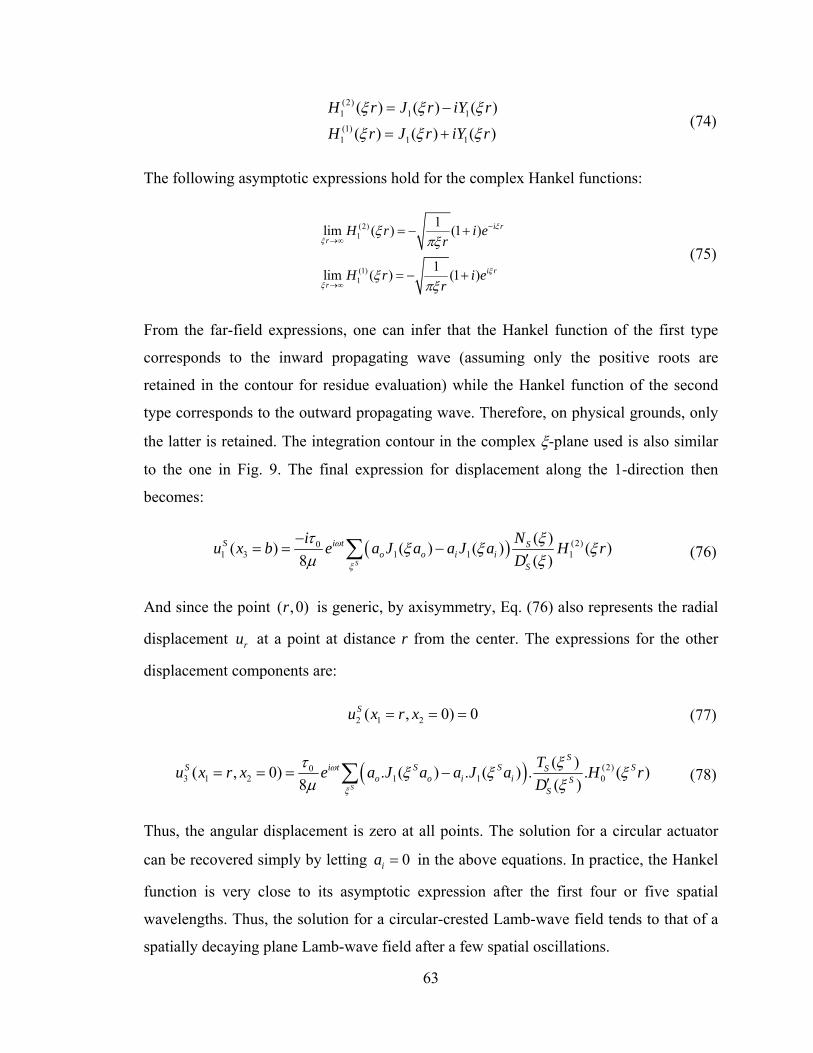
63
(2)1 1 1(1)1 1 1
( ) ( ) ( )
( ) ( ) ( )
H r J r iY r
H r J r iY r
ξ ξ ξ
ξ ξ ξ
= −
= + (74)
The following asymptotic expressions hold for the complex Hankel functions:
(2)1
(1)1
1lim ( ) (1 )
1lim ( ) (1 )
i r
r
i r
r
H r i er
H r i er
ξ
ξ
ξ
ξ
ξπξ
ξπξ
−
→∞
→∞
= − +
= − +
(75)
From the far-field expressions, one can infer that the Hankel function of the first type
corresponds to the inward propagating wave (assuming only the positive roots are
retained in the contour for residue evaluation) while the Hankel function of the second
type corresponds to the outward propagating wave. Therefore, on physical grounds, only
the latter is retained. The integration contour in the complex ξ-plane used is also similar
to the one in Fig. 9. The final expression for displacement along the 1-direction then
becomes:
( ) (2)01 3 1 1 1
( )( ) ( ) ( ) ( )8 ( )S
S i t So o i i
S
i Nu x b e a J a a J a H rD
ω
ξ
τ ξξ ξ ξ
µ ξ−
= = −′∑ (76)
And since the point ( ,0)r is generic, by axisymmetry, Eq. (76) also represents the radial
displacement ru at a point at distance r from the center. The expressions for the other
displacement components are:
2 1 2( , 0) 0Su x r x= = = (77)
( ) (2)03 1 2 1 1 0
( )( , 0) . ( ) . ( ) . . ( )8 ( )S
SS i t S S SS
o o i i SS
Tu x r x e a J a a J a H rD
ω
ξ
τ ξξ ξ ξµ ξ
= = = −′∑ (78)
Thus, the angular displacement is zero at all points. The solution for a circular actuator
can be recovered simply by letting 0ia = in the above equations. In practice, the Hankel
function is very close to its asymptotic expression after the first four or five spatial
wavelengths. Thus, the solution for a circular-crested Lamb-wave field tends to that of a
spatially decaying plane Lamb-wave field after a few spatial oscillations.

64
The harmonic out-of-plane displacement patterns due to excitation of the A0
Lamb mode at 100 kHz in a 1-mm Aluminum plate by rectangular, circular actuators are
shown in Fig. 11. Fig. 11a illustrates how the GW field due to a rectangular actuator
tends to a circular crested GW field with angularly dependent amplitude at some distance
from the actuator. In the far-field, it looks similar to the GW field due to a circular
actuator shown in Fig. 11 (b). In addition, one can appreciate the directionally focused
nature of the GW field from 3-3 APTs in Fig. 11 (c). The waves propagate in a roughly
collimated beam in a limited sector centered about the fiber direction. This directionality
is expected to be refined even more if the electrode pattern of the transducer is designed
in a comb-transducer like fashion, as shown in Fig. 11 (d). This can be achieved by
designing the clusters of electrode fingers spaced at intervals equal to half the wavelength
corresponding to the center frequency of the excited GW. Such a comb transducer also
has much better modal selectivity being more tuned to excite a particular wavelength
chosen by design.
While in this analysis it was assumed that a single angular frequency ω was
excited, it can be used to find the response to any frequency bandwidth-limited signal.
This can be accomplished by taking the inverse Fourier transform of the integral of the
product of the harmonic response multiplied by the Fourier transform of the excitation
signal over the bandwidth. In practice in GW testing, a limited cycle sinusoidal toneburst
is used, typically modulated by a Hanning window. If modulated by a Hanning window,
the excitation signal is of the form:
01 2( ) (1 cos )sin 22e
tV t f tTπ π= − (79)
where 0/(2 )T n f= is the duration of the toneburst, which is in practice an integral
multiple n of the half-period 01/(2 )f . The magnitude of the Fourier transform of this
signal, which gives the frequency content of the signal, is:

65
-0.8
-0.6
-0.4
-0.2
0
0.2
0.4
0.6
0.8
5 cm 5 cm
(a) (b)
-0.8
-0.6
-0.4
-0.2
0
0.2
0.4
0.6
0.8
5 cm -0.8
-0.6
-0.4
-0.2
0
0.2
0.4
0.6
0.8
5 cm
(d) (c)
Fig. 11: Harmonic radiation field (normalized scales) for out-of-plane surface displacement (u3) in a 1-mm thick aluminum alloy (E = 70 GPa, υ = 0.33, ρ = 2700 kg/m3) plate at 100 kHz,
A0 mode, by a pair of (a) 0.5-cm × 0.5-cm square piezos (uniformly poled, in gray, center); (b) 0.5-cm diameter circular actuators (in gray, center); (c) 0.5 cm × 0.5 cm square 3-3 APT (in grey stripes) with the fibers along the vertical direction and (d) 3-element comb array of 0.5 cm × 0.5 cm square 3-3 APT (in grey stripes) with the fibers along the vertical direction,
excited in phase

66
10 0
0 0 0
10 0
0 0
10
0 0
( ) sinc ( ) ( 1) sinc ( )4
1 1 1 + sinc ( ) ( 1) sinc ( )2
1 1 sinc ( ) ( 1) sinc (2
ne
n
n
n n nV f f f f ff f f
n n n nf f f ff n f n
n n n nf f ff n f
π π
π π
π π
+
+
+
⎛ ⎞ ⎛ ⎞= − + − + +⎜ ⎟ ⎜ ⎟
⎝ ⎠ ⎝ ⎠
⎧ ⎫⎛ ⎞ ⎛ ⎞− −⎪ ⎪− + − + +⎨ ⎬⎜ ⎟ ⎜ ⎟⎪ ⎪⎝ ⎠ ⎝ ⎠⎩ ⎭
⎛ ⎞++ − + − +⎜ ⎟
⎝ ⎠0
1 ) fn
⎧ ⎫⎛ ⎞+⎪ ⎪⎨ ⎬⎜ ⎟⎪ ⎪⎝ ⎠⎩ ⎭
(80)
where sinc( ) sin( )/( )≡ . The first two terms on the right-hand side in (80) correspond to
the contribution of the unmodulated sinusoidal toneburst and the last four terms are due
to the Hann window. The contribution of the first two terms alone and the contribution of
all the terms together on the right-hand side of Eq. (80) are plotted in Fig. 12. The effect
of the Hann window modulation is to double the width of the principal lobe while
significantly decreasing the side lobes and thus reducing the spread of the frequency
spectrum of the toneburst, as shown in Fig. 12. As it can be seen, the peak value is
0/(4 )n f , while the width of the principal lobe in the frequency domain of the modulated
toneburst is 04 /f n . These relations can be used to control the frequency bandwidth of
the excitation signal in order to reduce signal distortion due to dispersion1. This will
depend on what point on the group-velocity dispersion curve one is operating, which is a
function of the product of 0f and the half-plate thickness b. The response of any system
to a finite frequency bandwidth signal can be obtained by taking the inverse Fourier
transform of the system harmonic response to a forcing function of unit magnitude, Rh(f),
multiplied by the Fourier transform of the excitation signal ( )eV f over the frequency
bandwidth. For the Hann window modulated sinusoidal toneburst, the frequency
spectrum is concentrated mainly in the principal lobe, as seen in Fig. 12. This frequency
bandwidth is denoted as f∆ . Thus:
0
0
22
0
2
( ) ( ) ( )
ff
i fth e
ff
R f R f V f e dfπ
∆+
∆−
= ∫ (81)
1 Dispersion is a phenomenon wherein the original signal is distorted as it travels in a medium due to the different wavespeeds of its component frequencies.

67
This relation is used to find the theoretical magnitude of the response to a modulated
sinusoidal toneburst excitation signal employing the developed formulations for the
harmonic response.
II.5 Numerical Verification for Circular Piezos on Plates
In order to verify the result of the formulation proposed for isotropic plates, FEM
simulations were conducted using ABAQUS [205]. An infinite isotropic (aluminum
alloy) plate with a 0.9-cm radius piezo-actuator placed at the origin of the coordinate
system was modeled using a mesh of axisymmetric 4-noded continuum finite elements up
to a boundary at the radial position r = 15 cm. These were radially followed by infinite
axisymmetric elements placed at the boundary, which are used to minimize the reflected
waves returning from the boundary towards the origin. The FEM model represented only
half the plate thickness, and then a through-thickness symmetry or anti-symmetry
condition was applied to the mid-thickness nodes to model symmetric or anti-symmetric
modes, respectively. The actuator was modeled as causing a surface radial shear force at
f0-f0
0
0.25
0.5
0.75
1
-4 -3 -2 -1 0 1 2 3 4
Unmodulated
Modulated
f0-f0
04nf
08nf
02 fn
04 fn
Frequency
Four
ier t
rans
form
mag
nitu
de
Fig. 12: Frequency content of unmodulated and modulated (Hann window) sinusoidal tonebursts
68
= 0.9 cm, just as in the proposed formulation. A 3.5-cycle Hanning window modulated
sinusoidal toneburst excitation signal applied to the actuator was modeled by specifying
the corresponding waveform for the time variation of the shear force applied at r = 0.9
cm in the input file. The amplitude of radial displacement at r = 5 cm was recorded for a
range of values of the toneburst center frequency-plate thickness product. The mesh
density and the time step were chosen to be sufficiently small to resolve the smallest
wavelength and capture the highest frequency response, respectively (about 20 spatial
points per wavelength in the FEM mesh and 20 time steps per inverse frequency). Two
sets of simulations were performed: for symmetric and for anti-symmetric modes. These
were compared with the analytical predictions by the proposed formulation in Section
II.4.C (while considering the frequency bandwidth excited). The results are shown in Fig.
13. The FEM results compare very well with the theoretical predictions for both the S0
and A0 modes, providing verification for the proposed analytical formulation.
II.6 Piezo-sensor Response Derivation
In this section, the response of a uniformly poled surface-bonded piezo-sensor operating
in the 3-1 mode on a plate in a GW field and connected to a measuring device such as an
oscilloscope is derived. The relation between the electric field Ei, displacement Di and
internal stress in the piezoelectric element is [206]:
i ikl kl ik kE g Dσσ β= − + (82)
where iklg is a matrix of piezoelectric constants for the piezoelectric material, and
ikσβ are the impermittivity constants at constant stress of the piezoelectric material. Since
the impedance of the oscilloscope is usually very high (~ 1 MΩ), it can be assumed that
there is no electric current flowing between the sensor and the measurement device.
Therefore, 3 0D = . Furthermore, if the sensor is thin enough, 33 0σ ≈ . Thus, one obtains:

69
( )11
313 31 ( )
1c
ii iic
g YE g σ εν
−= − =
− (83)
where 11cY is the in-plane Young’s modulus of the sensor material, cν is the Poisson ratio
of the piezoelectric material, and εii is the sum of the in-plane extensional surface strains.
Note that the contracted notation has been used for the g-constant indices from Eq. (83)
onwards. Here it is assumed that the twisting shear stresses are negligible. The voltage
response of the piezo-sensor therefore is:
( )11
313
1 .1
c c
c cc c ii
c c cS S
Y g hV E h dS dSS S
εν
= − =−∫ ∫ (84)
where Sc is the surface area of the sensor and hc is the sensor thickness. This assumes the
electric field is uniform through the sensor thickness (satisfied for small thickness
piezos). An important assumption made here is that the sensor is infinitely compliant and
does not disturb the GW field. This is reasonably satisfied if the product of the sensor’s
thickness and Young’s modulus is small compared to that of the plate onto which it is
surface-bonded and it is of small size. For APTs used as sensors, a similar analysis holds,
Center frequency-plate half-thickness product (× 10-1 MHz-mm)
Nor
mal
ized
radi
al d
ispl
acem
ent a
mpl
itude
0
0.25
0.5
0.75
1
0 1 2 3 4 5
SimulationTheoretical
0
0.25
0.5
0.75
1
0 0.5 1 1.5 2 2.5
Simulation
Theoretical
Nor
mal
ized
radi
al d
ispl
acem
ent a
mpl
itude
Center frequency-plate half-thickness product (× 10-1 MHz-mm)
(a) (b)
Fig. 13: Comparison of theoretical and FEM simulation results for the normalized radial displacement at r = 5 cm at various frequencies for: (a) S0 mode and (b) A0 mode

70
except that they are only sensitive to extensional stress along their fiber direction. If the
Poisson effect is ignored, they are consequently insensitive to strains normal to the fiber
direction.
II.6.A Piezo-sensor Response in GW Fields due to Circular Piezos
Consider the response to harmonic excitation of a uniformly poled rectangular
piezo-sensor of width 2sθ in a GW field (excited by a circular piezo with 0ia = and
oa a= ) surface-bonded between r = rc and r = rc + 2sr. In this case, Eq. (84) becomes:
11 1131 31( ) ( )
(1 ) (1 )c c
c c c c r rc rr
c c c cS S
Y h g Y h g du uV rdrd rdrdS S dr rθθε ε θ θ
ν ν= + = +
− −∫∫ ∫∫ (85)
Suppose that the length of the piezo-sensor 2sr is small enough so that 2rd sθθ
θ ≈∫ over
the radial length of the sensor. Using this and Eqs. (76) and (85), one obtains (for
symmetric modes):
211(2)0 31
1 0( )( ) ( )
8 2 (1 ) ( )
c r
Sc
r sSi t S S Sc c S
c Sr c S r
a Y h g NV e J a H r drs D
ω
ξ
τ ξξ ξ ξ
µ ν ξ
+
=′− ∑ ∫ (86)
II.6.B Piezo-sensor Response in GW Fields due to Rectangular Piezos
Next, consider the response to harmonic excitation of a uniformly poled
rectangular piezo-sensor placed between the coordinates 1 2( , )c cx s y s− − and
1 2( , )c cx s y s+ + with its edges along the 1 2- and -x x axes in the GW field due to a
rectangular piezo-actuator described in Section II.4.A. In this case, Eq. (84) becomes:
( )1 2
1 2
11 1131 31 1 2
11 22 1 21 2 1 2 1 24 (1 ) 4 (1 )
c c
c c c
x s y sc c c c
c cc cS x s y s
Y h g Y h g du duV dS dx dxs s s s dx dx
ε εν ν
+ +
− −
⎛ ⎞= + = +⎜ ⎟− − ⎝ ⎠
∫∫ ∫ ∫ (87)

71
Using the asymptotic displacement expressions (from the method of stationary phase),
this leads to the following expression for sensor response in the far-field:
( )( ) ( )
110 31
21 2
41 2 1 22
2(1 )
sin( cos )sin( sin )sin( cos )sin( sin ) sin 2
SS
S i tSc c
SS ScS S
cS S S S
i r
N ei Y h gs s rDV
a a s s e
ω
ξξ π
ξτ πµ ν ξξ ξ
ξ θ ξ θ ξ θ ξ θθ
− +
⎛ ⎞−⎜ ⎟−⎜ ⎟′= ⎜ ⎟
⎜ ⎟×⎜ ⎟
⎝ ⎠
∑
(88)
This expression can be evaluated for 0θ = using L’Hospital’s rule to give:
( )( )
11( ) 40 31 2 1 1
1
sin( )sin( )2( 0)(1 ) 4
S
S
S S SSS i r tc c
c SSc S
Ni Y h g a a sV es rD
ξ ω π
ξ
ξτ ξ ξπθµ ν ξξ
− − +−= =
− ′∑ (89)
II.7 Setups for Experimental Validation and Results
To examine the validity of the theoretical expressions for the formulations
developed above, a series of experiments were done. Each of these involved aluminum
alloy specimens with three surface-bonded transducers. Two of these were at the center
on each surface of the structure and used as actuators while the third was at some distance
from the center and used as a GW sensor. Experiments were conducted to examine the
correlation between theoretical and experimental frequency response functions. The first
transmitted pulse sensed by a surface-bonded MFC sensor at some distance from the
center was monitored. Two sets of readings were taken. In the first set, the actuators were
excited in phase to excite symmetric modes while in the second they were excited out of
phase in order to excite the anti-symmetric modes. These actuators were powered with a
3.5-cycle Hanning-windowed sinusoidal toneburst over a range of center frequencies.
The highest excitation frequency was well below the cut-off frequency of the first
symmetric Lamb mode in the first set. In the second set, it was well below the cut-off
frequency of the first anti-symmetric Lamb mode and the first anti-symmetric SH-mode.
Thus, the S0 mode was predominantly excited in the first set while the A0 mode was
predominantly excited in the second set. Due to the piezo-actuator’s capacitive behavior,

72
its impedance varies with frequency, and so the actual voltage drop across it varies with
frequency. To account for this, the voltage amplitude across the actuator terminals was
also recorded for each reading and the sensor response amplitude and error estimate were
compensated accordingly. To obtain the theoretical sensor response to a Hanning-
windowed toneburst at a given frequency, one needs to evaluate the inverse time domain
Fourier transform over the excited frequency spectrum. The theoretical and experimental
signal amplitudes, normalized by the peak amplitude over the tested frequency range, are
compared over a range of frequencies for the S0 and A0 modes.
II.7.A Beam Experiment for Frequency Response Function of MFCs
A 1-mm thick aluminum alloy (Young’s modulus YAl = 70 GPa, Poisson’s ratio υ
= 0.33, density ρ = 2700 kg/m3) strip clamped at both ends was instrumented with three
MFCs, each 0.2 mm thick, as illustrated in Fig. 14. The actuators were excited with a 5 V
peak-to-peak signal and the average amplitude of the sensor response over 16 samples
was noted to reduce the noise levels. To predict the theoretical sensor response trend
versus frequency, one needs to use the value 2a = 3.2 cm (which is the length of the
active area of the MFC) in the expressions for beams. Only the contributions from the S0
mode were included for the first set. Similarly, only contributions of the A0 mode were
considered for the second set. The harmonic sensor response, found using Eq. (84) should
also be integrated over the frequency bandwidth of excitation for calculating the response
to a 3.5-cycle sinusoidal toneburst signal. The theoretical (also referred to as analytical)
and experimental results are compared in Fig. 15. Both curves are normalized to the peak
response amplitude over the considered frequency range.
II.7.B Plate Experiments for Frequency Response Functions of Piezos and MFCs
A 600 mm × 600 mm × 3.1 mm thick aluminum alloy plate (Young’s modulus YAl
= 70.28 GPa, Poisson’s ratio υ = 0.33, density ρ = 2684 kg/m3) was instrumented with a
pair of 6.5-mm radius, 0.23-mm thick PZT-5H circular piezo actuators at the center of the

73
plate on both free surfaces. A 10 mm (radial length) × 5 mm (width) × 0.3 mm
(thickness) PZT-5A rectangular piezo-sensor was surface-bonded at a radial distance rc =
50 mm from the center of the plate, as illustrated in Fig. 16 (a). Similar specimens were
built with surface-bonded rectangular piezos (Fig. 16 (b)) and MFCs (Fig. 17). The setup
was designed such that reflections from the boundaries would not interfere with the first
transmitted pulse received by the sensor over the frequency range tested, i.e., the infinite
plate assumption holds. As before, separate tests were done for symmetric and anti-
symmetric modes. These actuators were fed with a 3.5-cycle 9 V (peak-to-peak) Hanning
windowed toneburst. For each reading, the excitation signal was repeated at a frequency
1 mm
2 cm 1.5 cm
70 cm
3.2 cm
27 cm
35 cm
Aluminum strip MFC
0.2 mm
Fig. 14: Illustration of thin aluminum strip instrumented with MFCs
0
0.25
0.5
0.75
1
0 100 200 300 400 500
Center frequency of excitation (kHz)
Nor
mal
ized
sen
sor
resp
onse
am
plitu
de
Experimental
Theoretical
0
0.25
0.5
0.75
1
0 40 80 120 160
Center frequency of excitation (kHz)
Nor
mal
ized
sens
or re
spon
se a
mpl
itude
Experimental
Theoretical
(a) (b)
Fig. 15: Theoretical and experimental normalized sensor response over various frequencies in the beam experiment for: (a) S0 mode and (b) A0 mode

74
of 1 Hz (this was small enough so that there was no interference between successive
repetitions) and the averaged signal over 64 samples was used to reduce the noise levels
in the signal. The theoretical and experimental signal amplitudes, normalized by the peak
amplitude over the tested frequency range, are compared over a range of frequencies for
the S0 and A0 modes in Fig. 18. The error bars based on the standard deviation of the
amplitudes over the 64 samples (capturing 99.73% of the data points), and normalized by
the peak amplitude are also shown in Fig. 18. The time-domain experimental and
theoretical signals, also normalized to their respective peak amplitudes over the
frequency range, are compared in Fig. 19 for center frequency each in the S0 and A0
modes. The normalized theoretical and experimental amplitudes along with their
associated error bars are compared for the rectangular actuator experiment in Fig. 20
while the comparison of the normalized time domain signals is shown in Fig. 21 for one
center frequency in each mode. The corresponding frequency response curves for the
rectangular MFC experiment are shown in Fig. 22 and two time domain signals from this
experiment are shown in Fig. 23. The peak-to-peak excitation voltage for the MFC
experiment was amplified using a Krohn-Hite 7500 amplifier to 60 V, since the sensor
response was barely above the noise floor without using it, possibly due to the very small
actuator sizes.
II.7.C Laser Vibrometer Experiment
To test the theoretically-predicted focusing capability of the MFC along its fiber
direction in plate structures, an experiment was conducted using a Polytec scanning laser
vibrometer system that employed a Polytec OFV-303 sensor head and OFV-3001-S
controller. A 1-mm thick aluminum plate specimen with a pair of MFC actuators at the
center (of dimensions 2a1 = 1.5 cm, 2a2 = 2.8 cm) was used. The actuators were excited
with a 18 V peak-to-peak 3.5-cycle Hanning windowed sinusoidal toneburst signal.
However, for this experiment, the center frequency was kept fixed at 30 kHz and the
actuators were excited out-of-phase to excite the A0 mode predominantly. The laser
vibrometer measured out-of-plane surface velocity signals at a chosen point, and was
equipped with a computer-controlled scanning head (Polytec OFV-040) so that the scan
point could be swept with precision over the plate area. Signals were recorded over a grid

75
spanning a quarter section of the plate surface up to 20 cm from each symmetry axis,
since the field is expected to be symmetrical about the two axes in the plane of the plate.
The grid spacing was 0.6 cm along the fiber direction (which is a third of the A0 mode
wavelength at 30 kHz). Along the other direction in the plane of the plate near the
Piezo-sensor10 mm × 5 mm
Piezo-disc actuator
13 mm
50 mm
Al plate (600 mm × 600 mm)
3.1 mm
0.23 mm 0.3 mm
300 mm
Al plate (600 mm × 600 mm)
3.1 mm
0.3 mm 0.3 mm
Piezo actuator (25 mm × 5 mm)
35 mm
300 mm
35 mm
Piezo sensor (10 mm × 10 mm)
(a) (b)
Fig. 16: Experimental setups for frequency response validation of: (a) circular actuator model and (b) rectangular actuator model
Al plate (500 mm 500 mm)
Clamped boundary
MFC actuator (8 mm 5 mm)
MFC sensor (8 mm 5 mm)
50 mm
0.2 mm
3.2 mm 250 mm
Fig. 17: Experimental setup for frequency response validation of model for surface-bonded APTs on plates

76
0
0.25
0.5
0.75
1
1 1.5 2 2.5 3 3.5 4Center frequency ( X 100 kHz)
Experimental
Theoretical
Center frequency (× 100 kHz)
0
0.25
0.5
0.75
1
0 0.5 1 1.5 2 2Center frequency ( X 100 kHz)
Experimental
Theoretical
Center frequency (× 100 kHz)
Nor
mal
ized
sens
or r
espo
nse
ampl
itude
(a) (b)
Fig. 18: Comparison between experimental and theoretical sensor response amplitudes in the circular actuator experiment at different center frequencies for: (a) S0 mode and
(b) A0 mode
-0.4
-0.3
-0.2
-0.1
0
0.1
0.2
0.3
0.4
0.5
0 0.5 1 1.5 2 2.5 3
Time ( X 10 microsec. )
Nor
mal
ized
sens
or r
espo
nse
Experimental
Theoretical
A0 mode
Time (× 10 µsec.)
-0.6
-0.4
-0.2
0
0.2
0.4
0.6
0 2 4 6 8 10 1
Time ( X 10 microsec. )
Nor
mal
ized
sens
or r
espo
nse
Experimental
Theoretical
Time (× 10 µsec.)
(a) (b)
Fig. 19: Comparison between experimental and theoretical sensor response time domain signals for the circular actuator experiment: (a) S0 mode for center frequency 300 kHz
and (b) A0 mode for center frequency 50 kHz

77
0
0.25
0.5
0.75
1
1.25 1.5 1.75 2 2.25 2.5 2.75Center frequency (100 kHz)
ExperimentalTheoretical (actual dimensions)Theoretical (reduced dimensions)
Center frequency (× 100 kHz)
(nominal dimensions)
0
0.25
0.5
0.75
1
0 1 2 3 4 5 6 7 8Center frequency (10 kHz)
Experimental
Theoretical (actual dimensions)
Theoretical (reduced dimensions)
Center frequency (× 10 kHz)
(nominal dimensions)
(a) (b)
Fig. 20: Comparison between experimental and theoretical sensor response amplitudes in the rectangular actuator experiment at different center frequencies for: (a) S0 mode
and (b) A0 mode
-0.6
-0.4
-0.2
0
0.2
0.4
0.6
0 1 2 3 4Time (10 microsec.)
Nor
mal
ized
sens
or r
espo
nse
ExperimentalTheoretical (actual dimensions)Theoretical (reduced dimensions)
Time (× 10 µsec.)
A0 mode
(nominal dimensions)
-0.5
-0.4
-0.3
-0.2
-0.1
0
0.1
0.2
0.3
0.4
0.5
0 2 4 6 8 10 12Time (10 microsec.)
Nor
mal
ized
sens
or r
espo
nse
ExperimentalTheoretical (actual dimensions)Theoretical (reduced dimensions)
Time (× 10 µsec.)
(nominal dimensions)
(a) (b)
Fig. 21: Comparison between experimental and theoretical sensor response time domain signals for the circular actuator experiment: (a) S0 mode for center frequency 150 kHz
and (b) A0 mode for center frequency 50 kHz
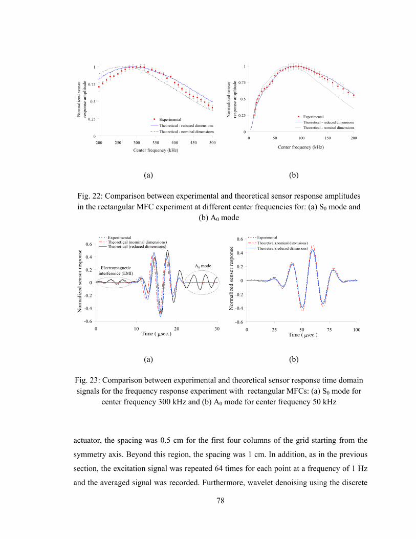
78
actuator, the spacing was 0.5 cm for the first four columns of the grid starting from the
symmetry axis. Beyond this region, the spacing was 1 cm. In addition, as in the previous
section, the excitation signal was repeated 64 times for each point at a frequency of 1 Hz
and the averaged signal was recorded. Furthermore, wavelet denoising using the discrete
0
0.25
0.5
0.75
1
200 250 300 350 400 450 500
Center frequency (kHz)
Nor
mal
ized
sens
or
resp
onse
am
plitu
de
ExperimentalTheoretical - reduced dimensionsTheoretical - nominal dimensions
0
0.25
0.5
0.75
1
0 50 100 150 200
Center frequency (kHz)
Nor
mal
ized
sen
sor
resp
onse
am
plitu
de
ExperimentalTheoretical - reduced dimensionsTheoretical - nominal dimensions
(a) (b)
Fig. 22: Comparison between experimental and theoretical sensor response amplitudes in the rectangular MFC experiment at different center frequencies for: (a) S0 mode and
(b) A0 mode
-0.6
-0.4
-0.2
0
0.2
0.4
0.6
0 10 20 30Time ( sec.)
Nor
mal
ized
sen
sor r
espo
nse
ExperimentalTheoretical (nominal dimensions)Theoretical (reduced dimensions)
µ
Electromagnetic interference (EMI)
A0 mode
-0.6
-0.4
-0.2
0
0.2
0.4
0.6
0 25 50 75 100Time ( sec.)
Nor
mal
ized
sen
sor r
espo
nse
ExperimentalTheoretical (nominal dimensions)Theoretical (reduced dimensions)
µ
(a) (b)
Fig. 23: Comparison between experimental and theoretical sensor response time domain signals for the frequency response experiment with rectangular MFCs: (a) S0 mode for
center frequency 300 kHz and (b) A0 mode for center frequency 50 kHz

79
Meyer wavelet was employed to cleanse the signals. The experimentally obtained surface
plots at three particular time instants over the quarter section of the plate are shown in
Fig. 24 (normalized to the peak value of surface velocity over the plate in the time span
up to 200 µs). The surface plots for the same GW fields obtained using the theoretical
model developed in this thesis are shown adjacent to these in Fig. 24. These are also
normalized to the theoretically predicted peak velocity over the plate area in the same
time span. These plots were generated assuming pure A0 mode excitation. SH-modes
were not considered since they do not cause out-of-plane displacements.
II.8 Discussion and Sources of Error
II.8.A Frequency Response Function Experiments
In the beam experiment, for the symmetric mode, the peak response frequency is
well captured by the model. In addition, the qualitative trend of the sensor response with
varying frequency is also captured. Similar conclusions hold for the anti-symmetric
mode. In this case, however, the peak response frequency is the lowest frequency of
testing. The qualitative prediction of the trend of the response is good, albeit with some
marginal quantitative error in the location and relative magnitude of peaks. The
frequency at which the second peak occurs is slightly over-estimated for both modes.
This error is possibly attributable to the use of uncoupled transducer-substrate dynamics
models in this thesis. Due to the relatively larger transducer to substrate thickness ratio
(in this case 0.2 mm to 1 mm), in order to obtain better accuracy in theoretical
predictions, models that account for the coupled dynamics will be needed. Some incipient
efforts in this direction can be found in Refs. [76] and [79].
In the plate frequency response experiment, there is qualitative agreement in the
trend between the theoretical and experimental results. There is some error observed in
the prediction of the peak frequency for the theoretical results in the experiments, and
they are particularly evident in the results for the rectangular piezo and MFC (for the
nominal transducer dimensions). However, the experimental results are in good
agreement with the theoretical curve for reduced transducer dimensions (by 20% for the

80
t = 100 µs
t = 100 µs
t = 150 µs
t = 150 µs
t = 200 µs
t = 200 µs
(a) (b)
Fig. 24: Normalized surface plots showing out-of-plane velocity signals over a quarter section of the plate spanning 20 cm × 20 cm. The MFC is at the upper left corner (the
striped rectangle), and its fibers along the vertical: (a) Experimental plots obtained using laser vibrometry and (b) theoretical plots obtained using the developed model for APTs

81
rectangular piezo and 13% along the fiber direction for the MFCs). This shift can be
attributed to the shear lag phenomenon, which relates to the assumption made in the
derivation pertaining to force transfer only along the free edges of the piezo. As
mentioned earlier, this “pin-force” model was proposed by Crawley and de Luis [85] for
the case of a pair of piezo-actuators surface bonded on opposite beam surfaces and
actuated quasi-statically. Due to the finite stiffness of the actuator relative to the plate and
imperfect bonding between the actuator and plate, the force transfer between the piezo
and the plate occurs over a finite length close to the edge of the piezo. Therefore, the
effective dimension in the models derived may be smaller than the actual physical
dimension. The circular piezo was thinner (0.23 mm) and more flexible (E = 59 GPa)
compared to the rectangular piezo (0.3 mm and 63 GPa), which possibly explains why
this effect was less noticeable in the former experiment. While the MFC was even thinner
(0.2 mm) and more flexible (E = 30.34 GPa), it is suspected that the presence of the
kapton electrode layer may have caused the shear lag effect to be greater than expected.
In addition, in the MFC experiment beyond about 375 kHz, the amplifier caused some
noticeable signal distortion in the amplified excitation signal which may have caused
some of the inconsistency at higher frequencies in the comparison between the theoretical
and experimental results for that set of results.
Another source of error comes from the impossibility of exciting a pure mode.
While there were two actuators bonded on either free surface at the center of the plate,
there would always be some mismatch in their piezoelectric properties due to
manufacturing imperfections. In addition, due to the finite thickness of the sensor, when
the wave packet is incident on it a small portion of the incident GW mode is converted to
other modes due to scattering. Because of this, it was verified that some excitation of
antisymmetric modes existed in the symmetric mode experiments and vice versa. An
effort was made to ensure that the time window over which the peak was recorded (using
the theoretical time-domain waveforms) was for the relevant mode of interest. In spite of
this, the results were significantly affected by the overlapping of the two modes over
certain frequency ranges, which were avoided.
82
The theoretical models all assume infinite substrates. This is accounted for in the
experiments by only examining the first transmitted pulse received by the sensor and
ignoring boundary reflections. In the beam experiment, due to the proximity of the sensor
to the boundary, some of the low frequency data for the first transmitted pulse is slightly
compromised by reflections from the boundary. At lower frequencies, due to the larger
time-spread of the excitation signal, the reflection tends to overlap with the first
transmitted pulse. This is more significant for the S0 mode due to the higher wavespeeds
at low frequency. These effects were significantly reduced in the plate experiments by
bonding the sensor closer to the actuators.
II.8.B Laser Vibrometer Experiment
The experimental surface out-of-plane velocity images obtained for the plate in
Fig. 24 (a) are also in good agreement with their theoretical counterparts. The
theoretically predicted focused nature of the GW field along the MFC fiber direction is
well captured in the experiment. There is also qualitative agreement in the patterns of the
weak radiation along the other directions. However, the amplitude for those is slightly
stronger in the experimental plots. In addition, the tendency of the GW field towards a
directionally dependent circular crested field in the far field, which was also predicted
theoretically, is evident in the experiment. There is some noise in the experimental plots,
despite the use of wavelet denoising. This is because the plate, in spite of lightly sanding
its surface, was a poor diffuse reflector in some areas when the laser was incident at an
angle. At such points, this was partially compensated by adjusting the focus of the laser’s
lens. Another minor source of error in correlation is the presence of a MFC sensor of size
0.9 × 0.5 cm2, 5 cm from the center. This may have caused weak scattering of the GW
field due to the slight change in local stiffness and mass induced by it.
Despite these sources of error, overall there is good correlation between the
experimental and theoretical results, thus providing validation for the derived models
describing GW excitation as well as the sensor response equation for surface-bonded
piezo-sensors.

83
II.9 Optimal Transducer Dimensions
This section discusses the use of the above analytical models for optimizing
transducer dimensions in various configurations.
II.9.A Circular Piezo-actuators on Plates
To optimize the actuator size for maximum sensor response to harmonic
excitation, everything in Eq. (86) is kept fixed except a. Then:
1( )cV aJ aξ∝ (90)
The right-hand side of Eq. (90) is an oscillating function of a with a monotonically
increasing amplitude envelope as seen in Fig. 25. The local maxima of cV are attained at
the corresponding local extrema of 1( )J aξ . Thus, there is no optimum value for
maximizing sensor response as such, and by choosing higher values of a that yield local
extrema, one can in principle keep increasing the magnitude of sensor response to
harmonic excitation. Notice that between any two successive peaks of the response
function there is a value for the actuator radius for which the response to harmonic
excitation is zero. This corresponds to a zero of the Bessel function. Although these zero
“nodes” caused by certain actuator radii are presented for simple harmonic excitation,
they have also a direct impact on a toneburst signal. One may take a toneburst center
frequency as responsible for most of the energy being delivered by the actuator. If the
product of the actuator radius and the toneburst center frequency coincides with a node as
shown in Fig. 25, then most of the signal will be attenuated.
Since the piezo-actuator has some capacitance, the harmonic reactive power
circulated every cycle raP is:
2 22 2022
a
r a aa
a
fk a VP fC V ah
π ε ππ= = ∝ (91)

84
where Va is the actuation voltage supplied to the piezo-actuator, f is the frequency of
harmonic excitation and the rest of the notation is analogous to that used for the piezo-
sensor. That is, the power circulation increases as the square of the actuator radius if all
other parameters are constant. Note that the dependence of the capacitance on driving
frequency and actuation voltage magnitude has not been considered (see [207], for
example). However these only tend to further increase the capacitance, and thereby the
reactive power circulation. This power being reactive is not dissipated, but is merely used
for charging the piezo in the positive half-cycle and is gained back when the capacitor is
discharged in the negative half-cycle. The power supply to drive the actuators will define
how much of this energy can be recycled.
In addition to this, the power source must supply the energy that is converted into
acoustic energy in the excited GW field. This is given by the expression:
( )ˆ.a
o
di ij
S
P n u dSσ= ∫ (92)
0
0.25
0.5
0.75
1
0 0.5 1 1.5 2 2.5
PowerResponse
Actuator radius a (× 10 cm)
Sens
or a
mpl
itude
Fig. 25: Amplitude variation of sensor response and power drawn to excite the GW field due to change in actuator radius for a 1-mm thick Aluminum plate driven harmonically in
the S0 mode at 100 kHz

85
where So is the cylindrical surface of thickness 2b and radius a centered at the origin, i.e.,
that encapsulates the region of the plate under the actuator. On substituting the
expressions for plate displacement and stress and evaluating the integral, an intricate
expression is obtained involving the plate material properties, plate thickness, the
actuator radius, and the excitation frequency/wavenumber. Intuitively, however, one
expects that this expression will also follow an oscillating trend with monotonically
increasing amplitude envelope as a function of actuator radius. This is confirmed in Fig.
25, where the peaks of the expression coincide with the peaks of the sensor response
curve. Evidently, the increased sensor response by actuator size tailoring is at the cost of
increased power consumption by the actuator.
In summary, the choice of actuator length for the largest local maximum is limited
by the power available to drive the actuator. Moreover, the area occupied by the actuator
on the structure as well as the desired area covered by the actuator-sensor pair signal
might be concerns that ultimately decide the actuator size.
II.9.B Rectangular Actuators
In the case of a surface-bonded rectangular piezo-actuator on a plate, due to the
highly direction-dependent GW field, this will depend on the angular location of the
piezo-sensor/region of interest for GW SHM on the plate relative to the piezo-actuator.
For example, consider the case 0θ = . If all parameters except 1a and 2a are kept
constant in Eq. (89), one obtains:
2 1sin( )S ScV a aξ∝ (93)
Thus, to maximize the harmonic sensor response of a piezo-sensor in the direction 0θ = ,
2a should be as large as possible. For 1a , any of the lengths given by the relation:
11 22 ( ) , 0,1, 2,3,...2 Sa n nπ
ξ= + = (94)
are equally optimal values in order to maximize sensor response. By an analysis similar
to the one in Section

86
II.9.A, it can be shown that the power requirement increases for larger actuator
dimensions. Thus, in order to minimize power consumption and the area occupied by the
actuator on the structure, the value of 1a is defined by Eq. (94) with 0n = . The choice of
2a will also be limited by similar concerns. A similar analysis holds for rectangular APTs
bonded on beams and plates.
II.9.C Piezo-sensors
Two particular configurations are studied for optimizing piezo sensor dimensions.
First, consider the Eq. (86) for the harmonic sensor response of a piezo in the GW field
due to a circular piezo-actuator. Assuming all parameters (except the sensor length 2sr) to
be constant:
2 2(2) (2)0( ) ( )
2 2
c r c r
c c
r s r so
cr rr r
H r H rV dr drs sξ ξ+ +
∝ ≤∫ ∫ (95)
This inequality holds due to the oscillatory nature of the Hankel function. Since (2)0 ( )H rξ is a monotonically decreasing function of r:
2 (2)(2) (2)00 0
( )( ( 2 )) ( )2
c r
c
r s
c r crr
H rH r s dr H rsξξ ξ
+
+ ≤ ≤∫ (96)
where the equality holds only at the limit of 2sr → 0. Thus, the maximum sensor response
is attained for 2sr = 0, and it decreases with increasing sr. This implies that the sensor
should be as small as possible to maximize |Vc| in the case of a circular-crested GW field.
A smaller sensor size would also interfere less with the GW field and is favorable from
the point of view of SHM system design, since the transducers should ideally occupy
minimum structural area. To validate this idea, the same setup as described in Section
II.7.B was used. However this time, a 20 mm (radial length) × 5 mm (width) × 0.3 mm
(thickness) sensor was surface-bonded at a distance of radius 50 mm from the plate center
so that rc = 50 mm, as before. The sensor’s radial length 2sr was reduced in steps of 0.5
cm by cutting the sensor on the plate with a diamond-point knife and examining the
response of its remaining part. For each length, an experiment along the lines of the

87
earlier ones was conducted for the S0 mode, i.e., the sensor response amplitudes were
measured over 64 samples for each center frequency over a range of center frequencies.
The comparison between the theoretical and experimental results is shown in Fig. 26
(both data sets are normalized to the peak value for the curve at 2sr = 2 cm). The
theoretical curves were derived assuming uniform bond strength over all of the original
piezo sensor’s area. As predicted by the theoretical model, the sensor response amplitude
increases with decreasing sensor length. The comparison between the theory and
experimental results is good again, although the experimental curve is slightly shifted
ahead of the theoretical curve along the center frequency axis due to shear lag. The
comparison between the relative amplitudes is quite accurate with the exception of the
last set for 2sr = 0.5 cm, which can be possibly attributed to weaker bond strength closer
to the edge of the piezo-sensor.
Now consider Eq. (88) for the far-field harmonic sensor response of a piezo in the
GW field due to a rectangular piezo-actuator. If all parameters except 1s and 2s are kept
constant:
1 2
1 2
sin( cos ) sin( sin )( cos ) ( sin )
S SS
c S S
s sVs s
ξ γ ξ γξ γ ξ γ
∝ ⋅ (97)
Since the function sin tt
is maximum at t = 0, and its subsequent peaks after t = 0 rapidly
decay, one concludes that for maximum sensor response amplitude (|Vc|) in the far-field,
the sensor dimensions, i.e., 2s1 and 2s2, should be as small as possible, preferably much
smaller than the half-wavelength of the traveling wave.
Similar analysis can be done for piezos/APTs bonded on beams/plates in the far
GW field excited/scattered by an arbitrary source to conclude that the smaller the sensor
size, the stronger its response. This is essentially due to the piezo-sensor’s mechanism to
be sensitive to the average strain over its surface area. When sensing a spatially
oscillating GW, this leads to a stronger response if the area over which the averaging is
done is smaller. How small the piezo can be made will be limited by shear lag, as
observed in the experiment above. Depending on the strength of the bonding mechanism,

88
0
0.5
1
1.5
2
2.5
3
0.5 1 1.5 2 2.5 3 3.5 4Center frequency ( X 100 kHz)
2 cm experimental1.5 cm experimental1 cm experimental0.5 cm experimental
2 cm theoretical1.5 cm theoretical1 cm theoretical0.5 cm theoretical
Center frequency (× 100 kHz)
Fig. 26: Comparison between experimental and theoretical sensor response amplitudes in the variable sensor length experiment
beyond a point reducing sensor size will cause the GW signal to be completely lost in the
bond layer. Another situation where this sensing mechanism can be exploited is when the
sensed signal is multimodal and immunity to one of the GW modes is desired. In that
case, if the sensor size is designed to be equal to the wavelength of that mode
corresponding to the expected center frequency of the signal, the contribution from that
mode will be negligible due to the sensor’s averaging mechanism. This can be exploited
to reduce the demands on the signal processing algorithm, as explored in Chapter IV.
Thus, in summary, in this chapter, 3-D elasticity models were developed for GW
transduction by piezos and these were validated by FEM and experiments. Some analysis
was also presented for tailoring transducer dimensions to maximize GW field strength
when used as actuators and also to maximize response amplitude as sensors. The next
chapter uses these models along with other concepts to provide a set of design guidelines
for transducers and the excitation signal in GW SHM systems.

89
CHAPTER III
DESIGN GUIDELINES FOR THE EXCITATION SIGNAL AND PIEZO-TRANSDUCERS IN ISOTROPIC STRUCTURES
In this chapter, the models developed in the previous chapter along with other
ideas are exploited to furnish a set of design guidelines for GW SHM systems,
specifically for the excitation signal and the transducers in isotropic structures. Fig. 27
shows a tree-diagram which lists the various parameters that need to be chosen for the
excitation signal and transducers in GW SHM systems. The next two sub-sections
prescribe the specific guidelines for excitation signal and transducer design. Each sub-
section in these begins with the guideline in italics, followed by the reasoning behind it.
Actuation signal
Transducer
Center frequency
Window design
Number of cycles
Configuration
Actuators SensorsShape
DimensionsMaterial/
Type
Mode selection
III.1.A
III.1.C
III.1.B,D
III.2.A
III.2.A
III.2.B
Spacing
III.2.D III.2.DIII.2.C,D
III.2.A
Dimensions
Material/ Type
GWSHM
III.1.A
III.1 III.2
Fig. 27: Tree diagram of parameters in GW SHM (numbers above/below the boxes indicate section numbers for the corresponding parameter)

90
III.1 Excitation Signal
In GW SHM, the excitation signal is typically a high-frequency pulse signal. This
feature distinguishes this approach from other vibration-based SHM schemes. If the
excitation signal is too long in the time-domain, the response of the structure might be
masked by multiple boundary reflections. Most commonly, a modulated sinusoidal
toneburst signal spanning a few cycles is used. The following guidelines should aid in
choosing the specifics of this signal.
III.1.A Center Frequency/GW mode
The center frequency and GW mode should be decided based on the damage types(s) of
interest, using relevant information of GW sensitivity studies for each damage type.
The center frequency of the excitation signal is a crucial parameter. Along with
the GW mode, it decides the wavelength, which in turns defines the minimum size of the
least sensitive of the different damage types which are hoped to be detected using the
GW SHM system. The wavelengths of the GWs are found from the dispersion curves.
Mode sensitivity to a damage can be found using FEM-based damage sensitivity studies
or from theoretical models that describe the GW-scattered field from the damage as
discussed in Section I.4.A. For example, by exciting a mode with a through-thickness
stress profile such that the maximum power is transmitted close to a particular interface
through the plate thickness, the plate can be scanned for damage along that interface.
Rose et al. [63] predicted through analysis of displacement and power profiles across the
structural thickness that in metallic plates the S0 mode would be more sensitive to detect
large cracks or cracks localized in the middle of the plate. On the other hand, the S1 mode
would be better suited for finding smaller cracks or cracks closer to the surface. Alleyne
and Cawley [66] found from FEM-based sensitivity studies that notches of depth of the
order of 1/40 times the wavelength could be detected by Lamb waves in a plate. They
also found that the sensitivity was independent of the size of the notch in the plane of the
plate, as long as the was small compared to the wavelength. Furthermore, it might be
useful to test at more than one frequency, since defects of some particular dimensions can
be insensitive to a given wavelength (see, e.g., Fromme et al. [73]).

91
The following types of structural damage/defects have been detected using GWs
in the literature: delaminations in composites [65], notches [66], impact damage (usually
in the form of an indentation or hole [73], structural cracks (which could be fatigue-
induced, e.g., [72], loss of material due to corrosion [208], cracks in welds [209], bolt
torsion in clamps/fasteners supporting structures [175], disbonds between skin and the
honeycomb core in sandwich structures [157], and disbonds at adhesive joints [173].
III.1.B Number of Cycles
Decide on the number of cycles in the toneburst based on a tradeoff study between blind-
zone area and dispersiveness.
There is always a small blind-zone area surrounding the transducers used in GW
SHM, where damage cannot be detected. The blind-zone area results because small
amplitude scattered GWs from damage sites going to the sensor cannot be easily
separated from the large amplitude first transmitted GW pulse from the actuator (or the
excitation signal if the actuator itself is being used as sensor) or from the GW reflections
from the boundary (which are also usually significantly larger compared to reflections
from damage sites). Therefore, from this standpoint, a smaller number of cycles will
decrease the blind zone area. On the other hand, a larger number of cycles will reduce the
frequency bandwidth, and thereby, decreases “dispersion.” Dispersion is a phenomenon
wherein the original signal is distorted as it travels in a medium due to the different
wavespeeds of its component frequencies. Therefore, the number of sinusoidal cycles in
the excitation signal has to compromise between these two factors. The former is
proportional to the square of the number of cycles for a given excitation frequency while
the latter reduces with increasing number of cycles due to the reduction of the main lobe
width in the frequency spectrum. Thus, if one is operating in a relatively non-dispersive
region of the dispersion curve, one could afford to use a fewer number of cycles.
III.1.C Modulation Window
Choose a Kaiser window for modulating the excitation signal.
To minimize the problem of dispersion created by using a finite time-duration
signal, it should be modulated by a window which minimizes the spread of the signal in

92
the frequency domain. The effect of truncating a harmonic signal is to smear its signal
energy in the frequency domain in a main lobe centered about the original frequency,
along with weaker side lobes. Modulation typically widens the main lobe and makes the
side lobes smaller. The Kaiser window approximates the prolate spheroidal window, for
which the ratio of the main-lobe energy to the side-lobe energy is maximized in the
frequency domain (Papoulis [210]). It is given by the expression:
2
0 2
0
41
( )( )
tI
k tI
βτ
β
⎛ ⎞−⎜ ⎟⎜ ⎟
⎝ ⎠= (98)
where 0 ( )I is the modified Bessel function of the first kind of order 0, τ is the duration
of the window (fixed by the number of cycles) and β is a parameter that controls the main
lobe width in the frequency domain. Let ∆ml be the chosen main lobe width defined by
the distance between the central zero-crossings in the plot of the magnitude of the Fourier
transform (see Fig. 28). Then the amplitude attenuation factor in dB of the main lobe to
the largest side lobe is:
155 1 1224
mlslA τ
π∆ −
= − (99)
The window parameter β is chosen to be:
0.4
0 13.260.76609( 13.26) 0.09834( 13.26) 13.26 60
0.12438( 6.3) 60 120
sl
sl sl sl
sl sl
AA A A
A Aβ
≤⎧⎪= − + − < <⎨⎪ + ≤ <⎩
(10
0)
That is, for 13.26slA ≤ , the Kaiser window reduces to the rectangular window.
III.1.D Consideration for Comb Array Configurations
When using a comb transducer, ensure that the main lobe in the frequency spectrum is
narrow enough so that higher harmonics of the primary wavenumber of interest are not
excited.

93
t ω
k(t) ( )K ω
Fourier transform
∆mlτ
Fig. 28: The Kaiser window and its Fourier transform
2 2x a=
2 2x a= −
2λ
2λ
(a) (b)
Fig. 29: Illustration of comb configurations: (a) using ring elements and (b) using rectangular elements
A comb configuration (Fig. 29) is an array of transducers that is equally tuned to
a particular wavelength of interest and its integer multiples (illustrated in Fig. 30).
Therefore, when using such a configuration, ensure that the excitation signal is such that
its frequency bandwidth does not include any higher harmonics of the wavelength of
interest. A more detailed description of comb transducers can be found in Section III.2.

94
III.2 Piezo-Transducers
III.2.A Configuration/Shape Selection
Choose the configuration of the transducer(s) and the individual transducer
shape(s)/type(s) to suit the application:
• For large area scanning from a central point on the structure, use multi-element
arrays.
• For small area scanning, use a few elements in pulse-echo or pitch-catch mode.
• For uniform radiation in all directions, use circular actuators.
• For focused radiation, use an appropriately designed rectangular piezo actuator.
• For unidirectional sensing, use an anisotropic piezocomposite transducer.
• For modal selectivity, use comb configurations.
0
0.25
0.5
0.75
1
0 100 200 300Frequency (kHz)
Normalized Induced Strain Amplitude
Single Actuator
8 actuator comb array
Fig. 30: Comparison of harmonic induced strain in A0 mode between an 8-array piezo comb transducer and that of a single piezo-actuator (power is kept constant).
The configuration and shape are highly dependent on the application area. For
example, if large area scanning from a central point of a structure without structural
obstacles (such as a reinforcement or joint) is desired, a linear phased or circular array
may be preferable. Phased arrays operate by scanning individual sector angles by
applying appropriate delays and scaling factors to the excitation signals to the individual
array transducer elements (see e.g., Purekar and Pines [123]). If however, a smaller area
is to be monitored, a simpler solution is to use a few transducers operating in the pulse-

95
echo configuration. A minimum of three transducers are needed for triangulation in a
plate or shell-like structure (this is further discussed in a subsequent chapter on signal
processing in this thesis). The pitch-catch configuration requires a denser network of
transducers in order to allow for triangulation. For beam-like structures, two transducers
in the pulse-echo configuration suffice to locate the damage. Note that the notion of
“small” and “large” areas depends on the material damping characteristics as well as the
power available per actuator. The relative spacing between sets of transducers on the
structure should be based on a calibration experiment to get an estimate of the range
capability of the chosen actuator/sensor configuration for the structure of interest and
actuation voltage levels.
The radiation patterns of a particular actuator depend on its shape. To ensure
uniform radiation in all directions in the plane of the plate, use circular actuators. This is
crucial in linear phased arrays, for example. If it is desired to monitor one or more
particular area(s) of the structure selectively, focused actuator shapes such as rectangular
ones are preferable. An APT may also be useful in this regard due to its preferential
direction of radiation along its fibers. However, care should be taken in their design since
these also excite horizontally polarized shear (SH-) modes along with Lamb modes, as
seen in the previous chapter. They are also advantageous to use in certain applications
due to their unidirectional sensing capability along the fiber direction. To achieve modal
selectivity and thereby easier signal interpretation, a comb configuration would be much
preferable.
III.2.B Actuator Size
Determine the optimal size of the actuator based on the theoretical model corresponding
to the particular chosen shape.
The formulas in this sub-section are based on theoretical models in the previous
chapter and assume the circulation power formula for harmonic excitation with capacitive
loads (in this case, the piezo-actuators), i.e., 22P fCVπ= . In practice, for modulated
sinusoidal tonebursts, the peak power drawn is close to this value. For more accuracy, a
correction factor can be used depending on the modulation window. It should be noted
that, since capacitive loads are reactive, this power is used in the positive half-cycle for

96
charging the capacitance and is gained back in the negative half-cycle when the
capacitance is discharged. The power dissipated in exciting the GW field in the structure
is neglected, since that is typically orders of magnitude smaller than the reactive power.
In addition, the nonlinear dependence of the capacitance of piezoelectric elements on
driving voltage and frequency is neglected (see e.g., Jordan et al. [207]). This should be
accounted for at high driving voltages (> 30 V). Sizing guidelines for circular and
rectangular uniformly poled piezos, rectangular APTs and ring-shaped/rectangular comb
actuators are presented in this sub-section. The objective of the design process here is to
maximize the GW field strength while remaining within the power, voltage and
maximum actuator size constraints of the system. The different parameters needed in the
formulas below are:
System constraints:
Vmax = Maximum actuation voltage that can be applied by the power source
P = Maximum power that can be supplied by the power source
amax = Maximum allowable actuator dimension
Actuator properties:
k = Dielectric ratio of the actuator material
ha = Thickness of actuator along the direction of polarization
Structural (substrate) properties:
E = Young’s modulus of the isotropic plate structure
υ = Poisson’s ratio of the isotropic plate structure
ρ = Material density of the isotropic plate structure
2b = Thickness of the plate structure
Other constants/parameters:
ε0 = Permittivity of free space
f = Center frequency of excitation
ξ = Wavenumber of the chosen GW mode at the operating center frequency

97
i) Circular actuator uniformly poled through thickness:
Let a be the variable corresponding to the radius of the circular actuator. Also,
consider the parameter 0a such that:
0max 0
12
aPhaV k fπ ε
= (10
1)
Fig. 31 illustrates the design space and the geometric locations of a0 and other parameters
that will be discussed for the circular actuator. Thus, 0a is the value of a at the
intersection of the power constraint curve and the line V = Vmax. If 0a < amax, which is
the maximum radius of an actuator permissible by the designer, then:
1. If 0a a= corresponds to an extremum of 1( )J aξ , then choose this value as actuator
radius.
2. If 0a a= does not correspond to an extremum of 1( )J aξ , let 2a correspond to the
first extremum of 1( )J aξ , such that 0 2 maxa a a< ≤ , if it exists (else choose 2 maxa a= )
and let 1a correspond to the maximum value of 1. ( )a J aξ for 00 a a< ≤ . If:
1 1 1 max 1 2 20
. ( ). ( ).2
aPha J a V J ak f
ξ ξπ ε
> (10
2)
then choose 1a a= . Otherwise, choose 2a a= . If 0 maxa a> , then choose the largest
maxima of 1. ( )a J aξ with max0 a a< ≤ , if such a maximum exists, else choose a to be
maxa .
The suggestions for circular actuator sizing are derived from the relation between the
GW strain or displacement field and actuator size/actuation voltage. As shown in the
previous chapter, if one is within the limits of the power supply, the GW strain field
strength for circular actuators is linearly proportional to 1. ( )Va J aξ (the linear
proportionality to V results from the linear dependence of 0τ on the actuation voltage V).
However, along the power constraint curve (defined by ( )202 .aVa fk h Pπ ε= ), since
Va is fixed, the field strength for circular actuators is linearly proportional to 1( )J aξ .

98
ii) Rectangular actuator uniformly poled through thickness
In this case, the dimensions depend on the direction(s) in the plane of the structure
where radiation is to be maximized. If, for example, it is desired to maximize radiation
along a particular direction while minimizing radiation perpendicular to it, then the
rectangular actuator should be oriented such that one of its two axes of symmetry is along
the direction of interest, say the 1x -axis. Let the dimensions of the actuator be 12a along
1x and 22a perpendicular to it, with 1 2a a< . Again, the formulas for the far-field GW
strain field are used in conjunction with the constraints to derive these recommendations.
Consider 2amax to be the maximum allowable actuator dimension. As shown in
Fig. 33, choose 2oa (the optimal value for 2a ) to be the largest zero of 2sin aξ such that
2 max0 a a< ≤ , if it exists. If no such zero exists then choose 2 maxa a= .
Let:
0 22 0 max8
aPhaa k fVπ ε
≡ (10
3)
If this value of 0a is larger than or equal to maxa , reset 0a to be maxa . If there exists a
corresponding to an extremum of 1sin aξ such that 00 a a< ≤ , then choose the smallest
value of ã for 1a . If such an extremum does not exist, and 0a was reset to amax, then
choose 1 maxa a= .
a
1
1
. ( ) ,
( )
a J a
J a
ξ
ξ
0
0.5
1
0 0.2 0.4 0.6 0.8 1
tavj
V
V.a = constant
1. ( )a J aξ
1( )J aξ
amaxa1 a0 a2
Vmax
Design space
a
1
1
. ( ) ,
( )
a J a
J a
ξ
ξ
0
0.5
1
0 0.2 0.4 0.6 0.8 1
tavj
V
1. ( )a J aξ
1( )J aξ
amaxa1 a0
Vmax
Design space
a2
20. 2aV a Ph k fπ ε=
Fig. 31: Parameters and design space for circular actuator dimension optimization

99
If such an extremum does not exist, and 0 maxa a< , then let ta be the first
extremum of 1 1(sin )a aξ such that 0 maxta a a< ≤ . If such ta does not exist, choose
maxta a= . If:
0 max2 0
sin( ). sin( ).8
at
t
Pha V aa a k f
ξ ξπ ε
> (104)
then the optimal value of 1a is 1 0oa a= , else choose 1o ta a= . The locations of these
parameters in the design space are shown in Fig. 34.
x2
x1
x3
2a2
2a1
0
0.5
1
1.5
2
0 0.2 0.4 0.6 0.8 1
tv
V2.a2 = constant2sin( )aξ
Design space
amax a2
Vmax
V
a2o
Fig. 32: Parameters and coordinate axes for rectangular actuator
Fig. 33: Choice of 2a for rectangular actuator
iii) Ring-shaped comb actuator uniformly poled through thickness
The possibility of using this configuration arises only if maxa , which is the
maximum allowable actuator radius, is larger than the value of a corresponding to the
second extremum of 1. ( )a J aξ . A comb configuration can be achieved by using
individual ring-shaped actuators or by using a large circular actuator with the necessary
electrode pattern etched on it. A comb configuration is much more preferable compared
to a circular actuator for axisymmetric GW excitation due to its modal selectivity. In
designing this, the maximum number of ring shaped actuators that can be used is 1n − ,
where n is the number of extrema of 1. ( )a J aξ for maxa a≤ . If n is odd and greater than 1,
there can be one circular actuator and 2n − ring-shaped actuators. If 1n = , only one

100
circular actuator can be used. The internal and external radii of the rings are the values of
a corresponding to the extrema of 1. ( )a J aξ . In choosing the number of ring actuators n,
the only issue preventing one from using the maximum possible number of elements
within the allowable actuator size is the drop in amplitude due to increase in capacitance
as more rings are used (which may cause reduced actuation voltage due to the finite
power supply of the system). Hence, the choice of n should be made after a careful
tradeoff study between tolerable dispersiveness and signal amplitude for each possible n.
0
0.5
1
1.5
2
2.5
3
3.5
4
0 0.2 0.4 0.6 0.8 1
t
v
f
V2.a1 = constant
2sin( )aξ
Design space
amax a1
Vmax
V
1 1sin( ) /a aξ
a0 at
1
1 1
sin( ),
sin( ) /
a
a a
ξ
ξ
0
0.5
1
1.5
2
2.5
3
3.5
4
0 0.2 0.4 0.6 0.8 1
t
v
f
V2.a1 = constant
2sin( )aξ
Design space
amax a1
Vmax
V
ã a0
1 1sin( ) /a aξ
1
1
sin( ),
sin( ) /
a
a
ξ
ξ
Fig. 34: Possible optimal choices of a1 for rectangular actuator in two possible cases
iv) Comb actuator with rectangular uniformly-poled piezos
Just as for the ring-shaped comb configuration, a rectangular comb-shaped
configuration (Fig. 29 (b)) is always preferable over a single rectangular actuator (if
maximizing radiation along one direction is desired). The possibility of using this
configuration arises if max32
a πξ
≥ . The individual rectangular actuator elements can be
designed using the guideline (ii) (note that the total power is equally split among the
elements of the comb array). If n is the number of extrema of sin aξ in the range
max maxa a a− ≤ ≤ (which is the number of half-wavelengths of the GW), then / 2n
identical rectangular actuators need to be used and placed between the same 2x -locations
( 2 2x a= and 2 2x a= − ), with their edges along the x1-locations being the odd multiples of
the half-wavelengths (see Fig. 29 (b)).

101
v) Rectangular APT actuators
For rectangular APTs used as actuators (which would be used for more strongly
focused GW fields than the corresponding uniformly poled rectangular piezo), the design
considerations are analogous to that for a rectangular uniformly poled piezo-actuator,
with 1a along the fiber direction.
III.2.C Sensor Size
Choose the sensor dimensions in the plane of the plate to be minimal, preferably much
smaller than the half-wavelength of the GW. If the signal processing algorithm cannot
handle multiple modes, design the sensor to be immune to the GW mode that is less
sensitive to the damage type(s) of interest.
As seen in the previous chapter, the sensor response keeps increasing as the
sensor dimensions in the plane of the plate are reduced, assuming the sensor is in the far-
field relative to the source (a distance of five to ten wavelengths). The only constraint on
decreasing sensor size is the phenomenon of shear lag wherein all the strain is taken by
the bond layer and nothing is transmitted to the sensor. However, with a reliable bond
layer, this limit can be stretched to a considerable extent. The exact smallest value
beyond which shear lag dominates may have to be determined experimentally for a
particular bonding mechanism2.
However, in making the sensor dimensions small, one should take care that the
signal processing algorithm in use can resolve and identify multiple GW modes. If this is
not possible, then the excitation frequency can be kept low enough so that only two GW
modes exist and the piezo-sensor can be designed to be immune to one of the GW modes.
This is done by choosing its size to be equal to the wavelength corresponding to the
center frequency for that mode. As discussed in Chapter II, due to the strain averaging
mechanism of piezo-sensors, this will almost nullify the contribution of that GW mode.
However, some mild contribution from that mode corresponding to the side bands of the
excited frequency bandwidth may still be present in the signal.
2In the author’s experience, using a two-part overnight setting epoxy (Epotek-301 from Epoxy Technology) with piezos of thickness 0.3 mm on a 3.2-mm aluminum plate, beyond an in-plane size of 0.5 cm, sensor size reduction does not yield any advantage.

102
Thus, it is evident that the optimal dimensions for sensors and actuators are quite
different. This implies that ideally separate actuators and sensors should be used for
improved signal performance. However, the final decision should be made in view of the
system architecture under consideration.
III.2.D Transducer Material
Choose the actuator material with the highest value for the product of in-plane Young’s
modulus and piezoelectric constant (the relevant d-constant) divided by the dielectric
constant. Use a sensor material with the highest value for the piezoelectric constant (the
relevant g-constant) and minimum material density.
The actuation authority of the piezo increases linearly with increasing values of
piezoelectric constant ( 31d or 33d depending on whether a piezo with isotropic poling or
an APT is used) and in-plane Young’s modulus ( 11aY or 33
aY ). The reactive circulation
power increases linearly with increasing dielectric constant k. Thus to maximize the
actuation capability per unit power drawn, the material with maximum value for the ratio 11
31aY d k (or 3333aY d k , as appropriate) should be chosen.
The sensor response strength is directly proportional to the product of the in-plane
Young’s modulus, the piezoelectric constant and sensor thickness. However, it is not
advisable to increase sensor thickness or Young’s modulus beyond a point. This may
cause the sensor to significantly disturb the guided wave field being sensed, and the
measured output will not be representative of the incident GW field. This is directly
related to the relative thickness and relative Young’s modulus of the sensor to the
substrate. Thus, for minimum interference with the GW field, PVDF sensor elements
would be more suitable due to their finer thickness and low in-plane Young’s modulus,
however their response strength is usually weak and often piezoceramics are preferred.
This relates to the classical problem of the science of measurements, wherein one has to
compromise between sensor readability and fidelity. However, an increase in the g-
constant does not perturb the field and at the same time increases sensor response. The
higher the material density, the greater the mass of the sensor, thereby perturbing the GW

103
field without any increase in the sensor response. Hence, the sensor material with
minimum material density is preferable.
The actuation signal and transducers, for which detailed recommendations were
provided in this chapter, are just two of the many pieces in GW SHM systems. There are
several other critical design issues involved in an effective GW SHM system. For
example, the bond layer should be thin, stiff (at the frequency of interest), uniform, and
robust to environmental conditions to ensure good transmission of strain between the
transducer and substrate. There are decisions concerning the electrical architecture, such
as whether wireless connections are needed. If wires are used, the connections should be
able to withstand electromagnetic interference and electrical noise (e.g., by using co-axial
cables). Several other such issues exist in other areas of GW SHM such as signal
processing, pattern recognition, actuation hardware, system reliability, transducer
diagnostics, etc. In many of these, because GW SHM is still evolving, it might not be
possible to obtain clear-cut design guidelines at this point. Some insights and
recommendations for the signal processing algorithm and the effects of elevated
temperature are presented in the following chapters.

104
CHAPTER IV
A NOVEL SIGNAL PROCESSING ALGORITHM USING CHIRPLET MATCHING PURSUITS AND MODE IDENTIFICATION
As alluded to in the introductory chapter, the objective of signal processing in
GW SHM is to extract information from the sensed signal to decide if damage has
developed in the structure, and if so, characterize it in terms of location. Information
about damage type and severity is also desirable from the signal for further prognosis.
However, classifying and quantifying damage usually requires some pattern recognition
algorithm which uses the output from the signal processing. This chapter addresses signal
processing by suggesting a new algorithm using chirplet matching pursuits and mode
identification. Problems associated with conventional approaches are described and the
potential to overcome those and automatically resolve and identify multimodal,
overlapping reflections is discussed. The algorithm, designed for pulse-echo based
methodologies, is tested using FEM simulations and experiments. Finally, the issue of in-
plane triangulation in isotropic plates is discussed.
IV.1 Issues in GW Signal Processing
To assess the issues involved in signal processing for GW SHM, results from a
couple of illustrative FEM simulations are presented. Consider a 2-D aluminum plate
structure, modeled using a finite element mesh of 2-D plane strain elements as shown in
Fig. 35(a) (the structure is infinitely wide normal to the plane of the paper). In the first
simulation, a notch is present. It is 0.5 mm deep and 0.25 mm across, at a distance of 7.5
cm from the plate center. There are surface-bonded thin piezoelectric wafer actuators on

105
7.5 cm 7.5 cm
2 piezos 1 cm long each, excited in S0 mode (simulated by shear traction at edge)
Notch
1 mm0.5 mm
Aluminum plate X-section
15 cm
6 cm 4 cm
2 piezos 1 cm long each, excited in S0 mode (simulated by shear traction at edge)
Notch 1
1 mm
0.5 mm
Aluminum plate X-section
12.5 cm
Notch 2
0.5 mm
2.5 cm
(a) (b)
0 1 2 3 4 5 6 7x 10⁻⁵
-4
-3
-2
-1
0
1
2
3
4 x 10⁻⁸
Time (s)
Surfa
ce a
xial
stra
in a
t the
cen
ter
Actuation signal
S0 reflection from notch
A0 reflection from notch
S0 reflection from boundary
0 1 2 3 4 5 6
x 10-5
-2
-1.5
-1
-0.5
0
0.5
1
1.5
2
2.5
3 x 10⁻⁸
Time (s)Su
rface
axi
al s
train
at t
he c
ente
r
Actuation signal
S0 reflection from notch 1
A0 from notch 1 + S0 from notch 2
S0 reflection from boundary
(d) (c)
Fig. 35: From top-left, clockwise: (a) 2-D plate structure with one notch; (b) 2-D plate structure with two notches; (c) surface axial strain waveform at the center for structure in
(b) and (d) surface axial strain at the center for structure in (a)
0
2
4
6
8
10
0 1 2 3
Frequency-plate thickness product (MHz)
Phas
e ve
loci
ty (x
100
0 m
/s)
A0 mode S0 modeA1 mode S1 mode
0
1
2
3
4
5
6
0 1 2 3Frequency-plate thickness product (MHz)
Gro
up v
eloc
ity (x
100
0 m
/s)
A0 mode S0 mode
A1 mode S1 mode
(a) (b)
Fig. 36: The Lamb-wave dispersion curves with circles marking the excitation center frequency for the FEM simulations: (a) phase velocity and (b) group velocity
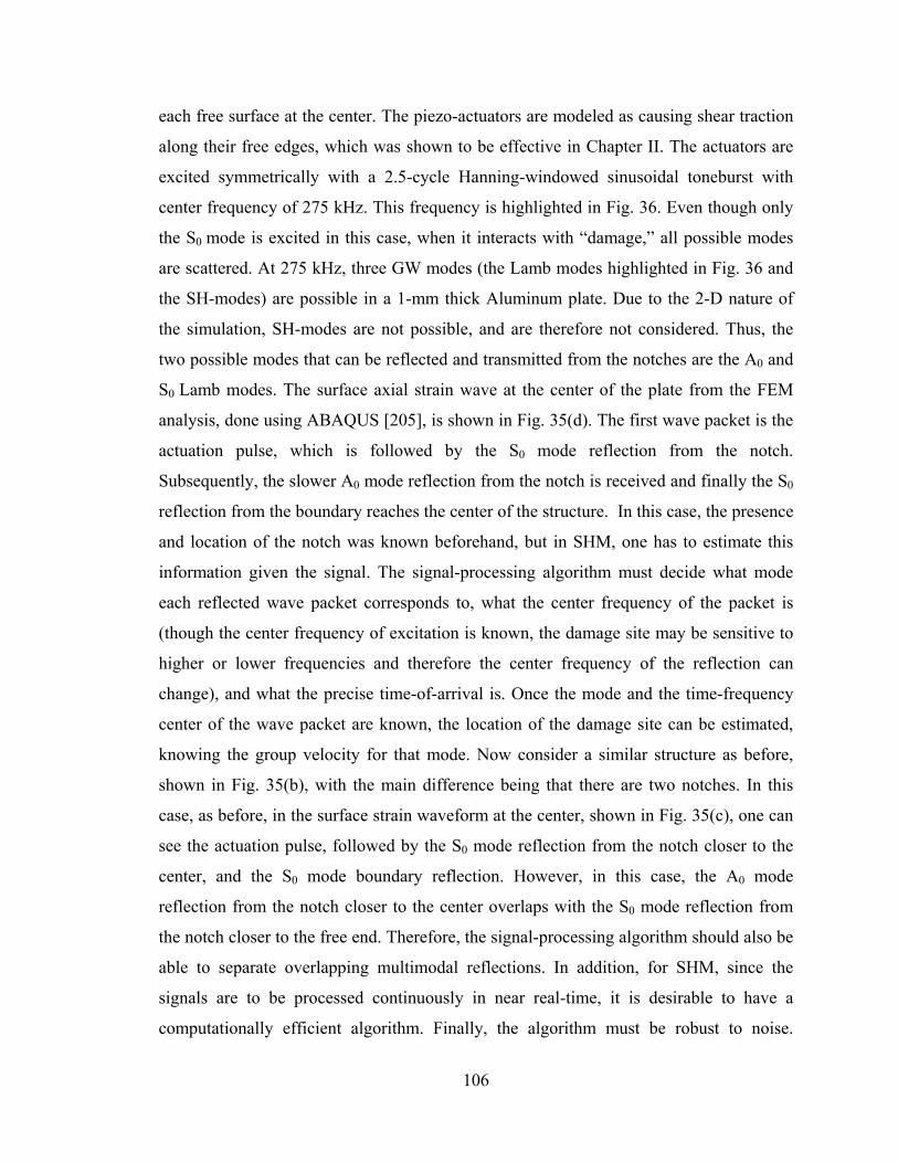
106
each free surface at the center. The piezo-actuators are modeled as causing shear traction
along their free edges, which was shown to be effective in Chapter II. The actuators are
excited symmetrically with a 2.5-cycle Hanning-windowed sinusoidal toneburst with
center frequency of 275 kHz. This frequency is highlighted in Fig. 36. Even though only
the S0 mode is excited in this case, when it interacts with “damage,” all possible modes
are scattered. At 275 kHz, three GW modes (the Lamb modes highlighted in Fig. 36 and
the SH-modes) are possible in a 1-mm thick Aluminum plate. Due to the 2-D nature of
the simulation, SH-modes are not possible, and are therefore not considered. Thus, the
two possible modes that can be reflected and transmitted from the notches are the A0 and
S0 Lamb modes. The surface axial strain wave at the center of the plate from the FEM
analysis, done using ABAQUS [205], is shown in Fig. 35(d). The first wave packet is the
actuation pulse, which is followed by the S0 mode reflection from the notch.
Subsequently, the slower A0 mode reflection from the notch is received and finally the S0
reflection from the boundary reaches the center of the structure. In this case, the presence
and location of the notch was known beforehand, but in SHM, one has to estimate this
information given the signal. The signal-processing algorithm must decide what mode
each reflected wave packet corresponds to, what the center frequency of the packet is
(though the center frequency of excitation is known, the damage site may be sensitive to
higher or lower frequencies and therefore the center frequency of the reflection can
change), and what the precise time-of-arrival is. Once the mode and the time-frequency
center of the wave packet are known, the location of the damage site can be estimated,
knowing the group velocity for that mode. Now consider a similar structure as before,
shown in Fig. 35(b), with the main difference being that there are two notches. In this
case, as before, in the surface strain waveform at the center, shown in Fig. 35(c), one can
see the actuation pulse, followed by the S0 mode reflection from the notch closer to the
center, and the S0 mode boundary reflection. However, in this case, the A0 mode
reflection from the notch closer to the center overlaps with the S0 mode reflection from
the notch closer to the free end. Therefore, the signal-processing algorithm should also be
able to separate overlapping multimodal reflections. In addition, for SHM, since the
signals are to be processed continuously in near real-time, it is desirable to have a
computationally efficient algorithm. Finally, the algorithm must be robust to noise.

107
Before the proposed algorithm is discussed, conventional solutions to the problem of GW
signal processing for SHM are first described and their shortcomings are highlighted.
IV.2 Conventional Approaches to GW Signal Processing
Conventional solutions to the problem of GW signal processing adapted from
NDT are usually in the form of some time-frequency representation (TFR). Unlike the
well-known Fourier transform, which provides “global” information about the frequency
content and is thereby suited for signals with stationary frequency content (meaning their
frequency content does not change with time), TFRs yield the “local” frequency content
and are better suited for non-stationary-frequency signals. The simplest example of a
TFR is the short time Fourier transform (STFT), in which the signal is divided into a
number of small overlapping pieces in the time domain, each piece is multiplied in time
using a fixed modulation window and the Fourier transform is used on the resulting
signal. Thus, the STFT, ( , )S t ω , of a signal, ( )s t , and the corresponding time-frequency
energy distribution, ( , )E t ω , obtained from it (called the spectrogram) are [211]:
21( , ) ( ) ( ) ( , ) ( , )2
iS t s h t e d E t S tωτω τ τ τ ω ωπ
∞−
−∞
= − =∫ (105)
where h(t) is the modulation window. Thus, an image is obtained for each point of the
time-frequency plane ( , )t ω . This TFR can be implemented quickly using the fast Fourier
transform (FFT) for digital signals. Another important TFR is the Wigner-Ville
distribution (WVD), which is defined as [211]:
*1( , )2 2 2
iW t s t s t e dωττ τω τπ
∞−
−∞
⎛ ⎞ ⎛ ⎞= + −⎜ ⎟ ⎜ ⎟⎝ ⎠ ⎝ ⎠∫ (106)
where * indicates the complex conjugate. An advantage of the WVD is that it can exactly
localize sinusoids, Dirac impulses and linear chirps. However, for other signals it always
has additional interference terms. Fig. 37 illustrates this point using the WVD of a signal
composed of two Gaussian modulated linear chirps. The interference terms can be

108
reduced by using a smoothing filter ( , )f t ω in the time-frequency plane. This yields the
generic smoothed WVD [211]:
( , ) ( , ) ( , )SW t f t W d dω τ ω ϖ τ ϖ τ ϖ∞ ∞
−∞ −∞
= − −∫ ∫ (107)
In fact, it can be shown that the spectrogram and energy distribution from all commonly
used TFRs such as the scalogram (which derives from the wavelet transform), the Hilbert
Huang spectrum, and others can be represented in the form of Eq. (107). The
disadvantage of smoothed WVDs is that they no longer can exactly localize linear chirps,
sinusoids and Dirac impulses. One always compromises between the interference terms
and time-frequency resolution. Further discussion on TFRs can be found in the books by
Cohen [211] and Mallat [212]. For GW signal processing, researchers typically use some
smoothed WVD followed by post-processing on the images. This isolates GW packets
and locates their time-frequency centers, spread in the time-frequency plane and total
energy. Finally, their modes are classified using the time-frequency “ridges” of the
reflections (these are the loci of the frequency centers for each time instant within each
reflection). Attempts by various researchers have tried this approach are reviewed in
Section I.5.B of Chapter I.
As an illustrative example, the spectrogram for the signal in Fig. 35b over the
excited bandwidth is shown in Fig. 38 (the modulation window used was identical to that
for the excitation signal). The spectrogram is plotted on a decibel scale (logarithmic) with
the peak value over the image as reference. For this simple example, the spectrogram
seems capable of isolating the individual reflections, identifying their time-frequency
centers and classifying their modes using the time-frequency ridges, which are
highlighted with white lines in each reflection. However, as it is shown in Section IV.5,
these are, in general, incapable of resolving overlapping multimodal reflections. Superior
TFRs that might be capable of resolving such overlapped signals typically have a high
computational cost associated with them. Another drawback of smoothed WVDs is
difficult automated post-processing. In addition, these are more suited for broadband
signals while in GW SHM, usually narrow-band signals are used, in order to minimize
signal spreading due to dispersion.

109
Another approach that has been tried for GW signal processing is the use of multi-
element sensor arrays. Some of these works are also reviewed in section I.5.B. In this
approach, the information about the spatial variation of the data over the sensing area of
the array is used to decide the mode of each reflection. That is, a multi-dimensional
Fourier transform is applied to the signals involving both time and spatial
transformations. However, a large number of closely spaced transducers to avoid aliasing
and sophisticated multi-channel data capture and processing hardware are needed to
implement this approach for GW SHM.
IV.3 Chirplet Matching Pursuits
The matching pursuits approach has already been introduced in section I.5.B. To
understand this algorithm, consider a complex valued signal 1( )f t that belongs to the
Hilbert space 2 ( )L R , where R is the set of real numbers. Suppose this space is an inner
product space with the inner product <.,.>. Then, the following hold:
2 *1 1 1 2 1 2( ) , ( ) ( )f f t dt f f f t f t dt
∞ ∞
−∞ −∞
= < ∞ =∫ ∫ (108)
where 2 ( )f t also belongs to 2 ( )L R . The property of finiteness of the 2-norm, defined by
the first expression in Eq. (108), also holds for 2 ( )f t . A dictionary D of all possible
expected wave structures, or “atoms,” is used, i.e., iD k= , where 2 ( )ik L R∈ and
1ik = . The 2-norm is also used as a metric of signal energy in this work. Then, the
matching pursuit algorithm decomposes a signal 2( ) ( )f t L R∈ into m atoms in the
following iterative way (with 0R f f= ):
(a) Choose the best atom in D:
1arg max ,m
i
mi i
k Dk R f k−
∈= (109)

110
(b) Compute the new residual after subtracting the component along the best atom
chosen in (a):
1 1 ,m m
m m mi iR f R f R f k k− −= − (110)
Thus, it decomposes the signal into a linear expansion of waveforms chosen to match
best the signal structure. Noise, in general, is uniformly distributed over the time-
frequency plane. Since the matching pursuit algorithm looks for concentrated energy
chunks in the time-frequency plane, it is inherently robust to noise. Due to this approach,
which is distinct from conventional TFRs, the time-frequency centers, the spread in the
time-frequency plane and the energy of the individual reflections are readily known, and
no post-processing needs to be done on the output. It becomes much easier to automate
this process in comparison to algorithms using conventional time-frequency
representations. In those solutions, to automate the process, image processing algorithms
would have to be used subsequent to the generation of the time-frequency plot to isolate
the individual reflections.
In the original paper on matching pursuits [112], an efficient algorithm using a
Gaussian modulated time-frequency atoms dictionary is described. This dictionary
consists of the atoms:
0 50 100 150 200 250-1
-0.5
0
0.5
1
Time (s)
Sig
nal a
mpl
itude
Time (s)
Freq
uenc
y (H
z)
50 100 150 200 250
0.1
0.2
0.3
0.4 Interference terms
-30
-25
-20
-15
-10
-5
0
Time ( s)
Freq
uenc
y (k
Hz)
10 20 30 40 50 60
100
200
300
400
500
µ
0S0 from
boundary dB
S0 reflection from notch
100
400
300
Actuation signal
A0 from notch
200
Fig. 37: WVD of two linear modulated chirps
Fig. 38: Spectrogram of the signal in Fig. 35 (d)

111
( )( ) ( )1 4 2( , , )
1( ) exp with ( ) 2 expl ut uk t g i t u g t t
llω ω π−⎛ ⎞= − = −⎜ ⎟⎝ ⎠
(111)
where u is the time center of the atom and ω is the angular frequency center of the atom.
Also, l is the scale of the atom, which is a metric representing the dilation along the time
axis of the Gaussian window ( )g t . It is indicative of the atom’s time-frequency spread.
These have stationary time-frequency behavior, i.e. the frequency at which the peak
energy occurs for each time instant does not change with time, as would be seen in a
WVD plot (see Fig. 39). Once the decomposition is done, it is possible to construct a
time-frequency plot of the constituent atoms without the interference terms obtained
using the conventional WVD. Thus, the resolution possible from such an approach is
always superior to that from conventional smoothed WVDs. In addition, the use of
Gaussian windows ensures that the atoms are optimal in terms of having minimal product
for the root-mean squared (RMS) pulse time-width and RMS frequency bandwidth [213].
The matching pursuit algorithm with this dictionary has been explored by some
researchers for GW signal analysis [114], [115]. However, the implicit assumption in
these works is that the signals are unimodal and non-dispersive. The atoms in this
dictionary are ill-suited for analyzing dispersive signals, which have non-stationary time-
frequency behavior. Furthermore, these atoms would not help in GW mode classification,
since different modes with the same energy at the same-time frequency center would
yield similar atoms.
Gribonval [116] proposed an algorithm for matching pursuits using a dictionary
consisting of Gaussian modulated chirplet atoms. That is, the dictionary comprises of
atoms of the form:
( ) ( )2( , , , )
1( ) exp2l u c
t u ck t g i t u t ullω ω− ⎡ ⎤⎛ ⎞ ⎛ ⎞= − + −⎜ ⎟ ⎜ ⎟⎢ ⎥⎝ ⎠ ⎝ ⎠⎣ ⎦
(112)
where c is the chirp-rate of the atom. These have linear time-frequency behavior (see Fig.
40). Once the GW signal is decomposed into chirplets, the additional parameter, i.e., the
chirp-rate, can be used to identify the modes of the individual reflections. This algorithm
is even more computationally efficient than the spectrogram. The computational time to

112
decompose an N-point signal into M atoms is O (MN), whereas the complexity involved
in generating the signal’s spectrogram, not including post-processing, is O (N2log2N).
Thus, the chirplet matching pursuit seems an attractive option for GW signal processing.
In the next section, a detailed outline of the overall algorithm proposed using the chirplet
matching pursuits approach is presented.
IV.4 Proposed Algorithm for Isotropic Plate Structures
IV.4.A Database Creation
This algorithm is designed for GW SHM in isotropic plate structures using the
pulse-echo method. That is, the structure has a central actuator excited with a high
frequency pulse and a collocated sensor receiving the GW echo pulses from the damage
sites, if any, and the boundaries. This presumes that a set of baseline signals is available
corresponding to the pristine condition for the structure. For this algorithm, initially a
database of the chirplet chirp-rates for the possible modes over the range of feasible time-
frequency centers must be generated. The frequency centers are limited to the bandwidth
excited in the structure, while the time centers are limited to the period between the end
of the excitation signal and the time taken for the slowest mode from the boundary to
reach the sensor. For this, it suffices to calculate these values for each mode at discrete
0.2 0.4 0.6 0.8
0.5
0
0.5
0.2 0.4 0.6 0.80
20
40
60
80
100
Time (s)
Freq
uenc
y (H
z)N
orm
. am
plitu
de
0.2 0.4 0.6 0.8
0.2 0.4 0.6 0.80
00
20406080
100
0
-0.5
0.5
0.2 0.4 0.6 0.8
0.5
0
0.5
0.2 0.4 0.6 0.80
20
40
60
80
100
Time (s)
Freq
uenc
y (H
z)N
orm
. am
plitu
de
0.2 0.4 0.6 0.8
0.2 0.4 0.6 0.80
00
20406080
100
0
-0.5
0.5
Fig. 39: A stationary Gaussian atom and its WVD
Fig. 40: A Gaussian chirplet and its WVD

113
points in the feasible region of the time-frequency plane. Then, use bilinear interpolation
if values for other points are needed. It should be mentioned that in this work the scale l
of the chirplet atoms in the dictionary was kept fixed. The chosen value of l, say 0l , was
such that the spread of the atom in the time-domain was slightly larger than that of the
excitation signal (20-30% larger by rule of thumb; however, for very dispersive signals,
this might need to be further increased). To generate the database, waveforms for each
mode at the discrete time-frequency points are generated assuming the defect is a point-
scatterer emitting circular-crested waves. These waveforms represent the expected
response of the piezoelectric wafer sensor collocated with the actuator. As discussed in
Chapter II, the response of a surface-bonded piezoelectric wafer is proportional to the
average in-plane extensional strain over its surface area (this assumes that the sensor is
thin and compliant enough to not affect the GW incident on it). For the FEM simulations,
the waveforms represent the surface displacement along the plate thickness direction at
the center of the plate. To do this, for each mode, the radial distance of the damage site
needs to be calculated. The phase velocity and group velocity curves for the isotropic
plate structure are assumed known. Suppose the S0 mode was excited predominantly (or
purely) and the excitation frequency is low enough so that the higher Lamb modes are not
possible. Since a narrow bandwidth pulse is used, the group velocity can be used as the
speed of pulse propagation to get damage site location estimates. Therefore, the radial
distance estimates for the possible modes at the time-angular frequency center 0 0( , )t ω
are:
( )
0 0 0
0 0
0 0
0 0 0 0 0
0 0
( / 2). ( ) ( / 2). ( ). ( );
2 ( ) ( )S S A
S A
e g e g gS A
g g
t t c t t c cr r
c c
ω ω ω
ω ω
− −= =
+ (113)
where et is the time-span of the excitation signal and 0( )gc ω is the group velocity of a
particular mode at angular frequency 0ω . Furthermore, a minor correction term equal to
half the actuator size along the direction of propagation is added to these estimates. This
is because, as seen in Chapter II, for surface-bonded piezoelectric actuators, the GWs
originate from the edge of the transducer, and not its center. Next, the wavenumbers for
each mode are calculated over the excited angular frequency range:

114
0 0
0 0
( ) ; ( )( ) ( )
S A
S Aph phc c
ω ωξ ω ξ ωω ω
= = (114)
It is assumed that after the GW excited by the actuator hits the damage site, it becomes a
point-source emitting circular crested waves axisymmetrically. The spatial variation of
the piezoelectric sensor response is therefore described by the Hankel function of order
zero (as seen for circular actuators in Chapter II). Since this wave is reflected from the
damage site back towards the collocated actuator/sensor, it is an incoming wave.
Therefore, if time dependence is of the form i te ω , then the Hankel function of the first
kind represents the incoming wave. For the case of symmetric mode reflection, the entire
distance 2 0Sr is traversed as symmetric mode (since it was assumed that the S0 mode was
predominantly excited). For the case of anti-symmetric mode reflection, half the total
distance 2 0Ar (from the actuator to the damage site) was traveled as S0 mode, whereas the
second half was traveled as the A0 mode. Therefore, the harmonic surface strain response
waveforms ( )Y ω for the two cases are (ignoring constants of proportionality, since only
the shape is of interest):
0 0
(1) (1) (1) (1)0 0 0 0 0 0 0 00 0 0 0( ) ( . ). ( . ); ( ) ( . ). ( . )S S S S S A S A A AY H r H r Y H r H rω ξ ξ ω ξ ξ= = (115)
Here the effect of the piezo sensor response being proportional to the average strain over
its surface area is neglected for simplicity. For the 2-D FEM simulations, the incoming
wave is given by the complex exponential function with positive exponent:
0 0 0 0 0 0 0 0 0 0
0 0
( 2 ) ( ). ; S S S S S S S A A Ai r i r i r i r rS AY e e e Y eξ ξ ξ ξ ξ+= = = (116)
The chirplet matching pursuit scheme uses a database of Gaussian atoms. Therefore, to
recover the time domain waveform ( )y t for a band-limited burst considering the
frequency bandwidth and Gaussian modulation, the following equations are used:
( ) ( )0
0
0
2 2(1)0 0 0 0 0
2
( ) ( ) . ( ) i tS S Sy t g l H r e d
ωωω
ωω
ω ω ξ ω∆+
∆−
= −∫ (117)

115
( )0
0
0
2(1) (1)
0 0 0 0 0 0 0 0
2
( ) ( ) . ( ). ( ) i tA S A A Ay t g l H r H r e d
ωωω
ωω
ω ω ξ ξ ω∆+
∆−
= −∫ (118)
where ∆ω is the angular frequency bandwidth and g( ) is the Gaussian window vector
centered at angular frequency ω and with the chosen scale 0l . A similar equation holds
for the 2-D FEM simulations. Of course, in practice, this is implemented in the discrete
(digital) domain. The inverse fast Fourier transform can be used for efficient
computation.
It should be noted that in this work, SH-modes were not considered for the
following reasons:
a) In the FEM simulations, the elements were 2-D, i.e., out-of-plane displacements
are not possible by design. Thus, SH-modes are not possible.
b) In the performed experiments, surface-bonded piezoelectric wafer transducers are
used as sensors, which are almost entirely insensitive to shear waves. This is
because they only sense the average in-plane surface extensional strain and not
shear strain, as mentioned before.
Once these waveforms are generated, the chirplet matching algorithm is applied to
them (restricting the scale of the dictionary chirplets to 0l ) and the chirp-rates
corresponding to each mode at each point of the time-frequency grid are obtained. The
chirplet matching pursuit was implemented using LastWave 2.0 [215], which is freeware.
Thus, one has the database required to use the proposed algorithm for GW signal
processing, which is described next.
IV.4.B Processing the Signal for Damage Detection and Characterization
The signal-processing procedure consists of the following steps:
i) The chirplet matching pursuit algorithm is applied to the difference between the test
signal and the signal for the undamaged state. A dictionary of chirplets with fixed

116
scale 0l as discussed in Section IV.4.A is used. Thus, the dictionary consists of
signals of the form:
( ) ( )2( , , )
00
1( ) exp2u c
t u ck t g i t u t ullω ω
⎛ ⎞− ⎡ ⎤⎛ ⎞= − + −⎜ ⎟ ⎜ ⎟⎢ ⎥⎝ ⎠⎣ ⎦⎝ ⎠ (119)
where the time center u is between the end of the first transmitted pulse received by
the sensor collocated with the actuator and the start of the boundary reflection while
the angular frequency center ω is within the excited angular frequency bandwidth.
This yields the time-frequency centers 0 0( , )t f , the chirp-rates 0( )c and the signal
energies of the constituent atoms (note that 0 02 fω π= ).
ii) The algorithm is run until the last atom extracted has energy above a certain
percentage of the first and most energetic extracted atom. In this work, this
percentage was chosen to be 10%. In the author’s experience, atoms below this
threshold tend to correspond to approximation errors.
iii) The most energetic atom in the time-span not corresponding to the excitation signal
or boundary reflections is examined. If it has energy above a certain threshold, the
structure is judged damaged. There is no hard and fast rule to decide the value of
this threshold, which is a critical parameter. The decision is dependent on the
energy in the signal difference corresponding to the excitation time interval. In
practice, no signal generator will be able to reproduce an excitation signal with
100% accuracy, and there is always some difference in the excitation signal as seen
by the collocated sensor3. In this work, the threshold was set to be 50% of the
energy in the excitation signal difference. This might need to be lowered for
structures with stronger damping characteristics. In addition, for the final SHM
system, this threshold must also take into account false positive/false negative
probabilities and risk assessment, which are highly application dependent.
iv) Next, mode identification is done using the atom’s chirp-rate. It is compared with
that of the possible modes for the same time-frequency center in the database. The
3 Due to the impossibility of perfect reproduction of the excitation signal, there is a small blind zone in the vicinity of the collocated actuator-sensor pair. This is associated with the sensor being unable to distinguish the small amplitude GW reflections from damage sites that might be very close to the actuator from the strong first transmitted pulse from the actuator.

117
mode is identified as the one that minimizes the absolute value of the difference
between the atom’s chirp-rate and the chirp-rate for each mode at the same time-
frequency center.
v) Knowing the mode and time-frequency center of each atom, the damage site’s
radial location relative to the transducer is known. Although damage-type
classification was not addressed in this work, the damage can then be characterized
by using the frequency center, the energy in the reflection from the damage site, and
the relative modal contributions from the damage site. This information can be used
to infer what the damage type is in conjunction with an artificial neural network
trained using prior experimental data or some modeling studies.
The proposed algorithm is summarized in the flowchart depicted in Fig. 41.
IV.5 Demonstration of the Algorithm's Capabilities
IV.5.A FEM Simulations
In Section IV.2, it was seen that the spectrogram was capable of isolating the
individual reflections and identifying their modes for the simple case of the GW signal in
Fig. 35 (d). Now consider the more complex signal in Fig. 35 (c), with overlapping
multimodal reflections. The portion of the signal between the end of the excitation signal
and the start of the boundary reflection, after artificial corruption with white Gaussian
noise (of amplitude 5% of the peak value in the signal), is shown in Fig. 42 (a). The
spectrogram for this signal (again, using a modulation window identical to that in the
excitation signal) is shown in Fig. 42 (b), on a decibel scale relative to the peak value in
the image. The spectrogram cannot separate the overlapping multimodal reflections from
the two notches, which are smeared together in the spectrogram. The time-frequency plot
from the chirplet decomposition using the matching pursuit algorithm is shown in Fig. 42
(c), also on a decibel scale. The power of this approach is evident from this figure, where
clearly the individual overlapping reflections from the two notches are resolved. In
addition, as highlighted in Table 1, the modes of the individual reflections are correctly
identified and the axial locations of the notches are identified with a maximum deviation

118
of 0.6 cm, or 6% of the distance from the transducer. For the two reflections that the
spectrogram could isolate, the errors for radial estimates are greater than that from the
proposed algorithm. Thus, the proposed algorithm shows superior resolution compared to
the spectrogram.
START
Read difference signal
Process with chirplet MP algorithm
Does first atom’s energy exceed
threshold?
Structure is undamaged
NO
Structure is damaged
YES
Identify atoms’ modes using chirp-rates
STOP
Atoms’ energies, time-freq. centers,
chirp-rates
Database of wavespeeds
Database of chirp-rates for modes
Compute damage locations
Damage locations
Fig. 41: Flowchart of proposed signal processing algorithm

119
IV.5.B Experimental Results
In order to verify the proposed algorithm’s potential capabilities, experiments
were conducted with a 1-mm thick Aluminum plate structure, the schematic of which is
shown in Fig. 43 (a). The 1-mm thick aircraft-grade Aluminum alloy plate was supported
on two support struts on two edges and the other two edges were free. Surface-bonded
PZT-5A piezoceramic transducers were used. The actuators were excited symmetrically
with a 2.5-cycle Hanning-windowed sinusoidal toneburst of center frequency 175 kHz,
10 20 30 40 50-2
-1.5
-1
-0.5
0
0.5
1
1.5 x 10⁻⁸
Time ( s)
Surfa
ce a
xial
stra
in
µ
(a)
-30
-25
-20
-15
-10
-5
0
Time ( s)
Freq
uenc
y (k
Hz)
10 20 30 40
200
400
600
µ
0
600S0 from N2 + A0 from N1
dB
S0 reflection from N1
200
400
-30 dB
0
-15
-10
-5
-20
-25
20 30 400
200
400
600
Time (µs)
Freq
uenc
y (k
Hz) S0 reflection
from Notch 1
S0 reflection from Notch 2
A0 reflection from Notch 1
(b) (c)
Fig. 42: (a) Portion of signal in Fig. 35 (c) with overlapping multimodal reflections and corrupted with artificial noise; (b) Spectrogram of the signal in (a); (c) Interference-free
WVD of constituent chirplet atoms for the signal in (a)

120
thereby predominantly exciting the S0 mode. After baseline signals were recorded for the
pristine condition, artificial “damage” sites in the form of C-clamps were introduced,
seen in Fig. 43 (b). The C-clamps act as local scatterers of GWs incident on it over their
contact area, causing incident GWs to be scattered from them. Damage in the structure,
such as cracks, dents or impact damage would also have a similar effect on GWs incident
on it. The difference signal between the pristine and “damaged” cases is shown in Fig. 44
(a). Again, in this case, the spectrogram, shown in Fig. 44 (b), is incapable of resolving
the overlapping S0 mode reflections from the two clamps. On the other hand, the
proposed algorithm showed its superior resolution in this case too. The chirplet matching
pursuit step was able to resolve the overlapping S0 mode reflections as well as the S0 and
A0 mode reflections from the boundary, as seen in shown in Fig. 44 (c). The second step
correctly identified the modes, thereby allowing accurate radial location estimates of the
clamps, as seen in Table 2 (Errors in location: C1 - 0.3 cm; C2 - 0.9 cm). The
spectrogram’s estimated location (for the reflection from the clamp that it could localize)
has the same error as the proposed algorithm. When using the relative modal
contributions to characterize the damage site, one must bear in mind that a finite-
dimensional piezoceramic sensor has different sensitivities to different wavelengths of
the GW sensed. As a first-order approximation, it might suffice to normalize the energy
Chi-rplet
#
t0 (µs)
fo (kHz)
c (kHz /µs)
Signal energy
(2-norm)
cA0 (kHz /µs)
cS0 (kHz /µs)
Mode r actual (cm)
r from new algo.
(cm)
r from spect. (cm)
1 41.6 245.9 -13 1.4× 10⁻¹⁴ -12.5 0.6 A0 6.0 6.4 6.5
2 38.4 319.6 34 3.7× 10⁻¹⁵ -10.2 0.5 S0 10.0 9.4 -NA-
3 25.6 280.8 7.4 1.8× 10⁻¹⁵ -7.9 0.3 S0 6.0 5.9 6.3
Table 1: Simulated notch damage in FEM simulation (Key: cA0 ≡ chirp-rate from database assuming A0 mode reflection; cS0 ≡ chirp-rate from database assuming S0 mode reflection; Mode ≡ identified mode; r actual ≡ actual radial location of notch; r from new
algo.≡ estimate of radial location of notch from proposed algorithm; r from spect. ≡ estimate of radial location of notch from spectrogram)

121
of each reflection to the sensitivity of the sensor to the wavelength corresponding to the
center frequency for the GW mode of the reflection (which can be obtained using the
theoretical model for piezo-sensor response in Chapter II).
It should be noted that the best accuracy in radial location estimation was in the
FEM simulation with the S0 mode reflection from N1 (error: 0.1 cm). There are two
reasons for this: (i) the reflection was isolated (i.e., not overlapping with another
reflection) and (ii) the notch was very thin axially (0.025 cm), and hence the “point-
scatterer” damage site model was realistic. In the experiment, the clamp had a contact
diameter of 1 cm, weakening this assumption, as reflected in the location errors.
Furthermore, the error tends to be worse for the weaker reflection in overlapping
reflections, as one would naturally expect. Another error source is the uncertainty in
material properties, which affects wavespeeds. Despite these errors, which are minor, the
advantages of the new algorithm over conventional approaches to GW signal processing
can be clearly seen with these results. However, it should be pointed out that testing was
restricted to the fundamental GW modes in this work. At higher frequencies, in the
presence of higher GW modes, the use of linear chirplets may not suffice. Quadratic or
higher order chirplets might need to be employed, such as in the work by Hong et al.
Actuator (2 cm ×0.5 cm)
8.2 cm10 cm
Sensor (2 cm ×0.5 cm)
2 cm
C- clamp contact diameter = 1 cm
C1
C2
1 mm
30 cm × 30 cm Al plate1 cm
1 cm
Support struts
15 cm
0.3 mm
(a) (b)
Fig. 43: (a) Schematic of experimental setup and (b) Photograph of experimental setup

122
[214]. In that work, the matching pursuit approach was used with quadratic chirp
functions for GW signal processing. However, in that work, sensing was restricted to one
mode there (by controlling the number of coil turns in the magnetostrictive GW sensor
used) and mode classification was not addressed. It should be noted that in this work, the
two modes had different dispersion characteristics over the excited frequency bandwidth.
If the two modes are similar to each other in terms of variation of wavespeed with
frequency, the chirp-rates for the two modes may be very close to each other. The
algorithm presented here may not be able to distinguish the modes. Until this point, only
radial location of damage sites relative to a transducer pair has been discussed. In the next
section, triangulation using multiple transducers in isotropic plates is discussed.
Chi-rplet
#
t0 (µs)
fo (kHz)
c (kHz /µs)
Signal energy
(2-norm)
cA0 (kHz /µs)
cS0 (kHz /µs)
Mode r actual (cm)
r from new algo.
(cm)
r from spect. (cm)
1 67.2 221.5 7.8 7.3 × 10⁻³ -5.11 0.14 S0 bndry bndry bndry
2 38.4 190.9 1.7 2.9 × 10⁻³ -4.55 0.07 S0 8.2 8.5 8.5
3 14.4 234.2 7.7 1.9 × 10⁻³ -1.79 0.01 Exctn
4 62.4 208.3 0.0 1.8 × 10⁻³ -5.17 0.13 S0 bndry bndry Bndry
5 100.8 166.1 -7.6 9.4 × 10⁻⁴ -4.63 0.33 A0 bndry bndry Bndry
6 48.0 208.3 0.0 9.2 × 10⁻⁴ -4.76 0.09 S0 10.2 11.1 -NA-
Table 2: Experimental results of isotropic plate with simulated damage (Key: cA0 ≡ chirp-rate from database assuming A0 mode reflection; cS0 ≡ chirp-rate from database assuming S0 mode reflection; Mode ≡ identified mode; r actual ≡ actual radial location of clamp; r
from new algo.≡ estimate of radial location of clamp from proposed algorithm; r from spect. ≡ estimate of radial location of clamp from spectrogram; bndry ≡ boundary
reflection; Exctn ≡ difference in excitation signal)

123
IV.6 Triangulation in Isotropic Plate Structures
In order to pinpoint the in-plane location of a damage site in an isotropic plate
structure and characterize it, one needs the radial locations of the damage site relative to
at least three pairs of central collocated piezoelectric transducers. It is highly desirable to
use circular or ring-shaped transducer wafers, so that there is no directional selectivity or
preference. In addition, care must be taken to use as thin piezoelectric wafers as possible
to minimize the extraneous reflections caused by the increased local stiffness of the
0 20 40 60 80 100-0.025
-0.02
-0.015
-0.01
-0.005
0
0.005
0.01
0.015
0.02
Time (microseconds)D
iffer
ence
sig
nal (
V)D
iffer
ence
sig
nal (
V)
Time (µs)
(a)
-30
-25
-20
-15
-10
-5
0
Time ( s)
Freq
uenc
y (k
Hz)
20 40 60 80 100
100
200
300100
300
Reflections from C1 and C2 smeared together
dB
µ
0
(b) (c)
Fig. 44: (a) Difference signal between pristine and “damaged” states; (b) Spectrogram of the signal in (a) and (c) Interference-free WVD of constituent chirplet atoms for the
signal in (a)

124
structure where the transducer is bonded. The proposed algorithm needs to be repeated
for the signals obtained using each collocated actuator/sensor pair. If there are multiple
mode reflections observed from the damage site, the average radial location obtained
from the modes can be used. One can then draw three circles of radii equal to the radial
locations thus found, about the centers of the corresponding actuator/sensor pairs. The
intersection of the three circles would yield the location of the damage site. This is
illustrated in Fig. 45 (a). In addition, as before, the relative modal contributions, the
frequency center and individual modal energies can be as input parameters for a pattern
recognition algorithm used to classify the damage and quantify its severity.
If however, one is mainly interested in locating damage and not in characterizing
it, an easier approach can be adopted. Instead of using three collocated piezoelectric
actuator/sensor pairs, it suffices to use three circular piezoelectric wafer transducers, and
while one is excited, the others can be used as sensors. However, in this approach, one
must ensure that the elements are sensitive only to one mode when used as sensors. Then,
the chirplet matching pursuit step is used to find the time-of-flight from the actuator to
the damage site and back to one of the sensors as well as the frequency center of the
pulse. This yields the distance traveled by the pulse, say d (since only one group velocity
is possible). The locus of all possible locations of the damage site is an ellipse with the
actuator and the sensor as its foci and d as the major axis. By exciting each actuator in
turn and using the others as sensors, three such ellipses can be drawn and the damage site
is located at their intersection. This concept was proven experimentally using a 3.15-mm
thick Aluminum 5052 alloy plate instrumented with three surface-bonded piezoelectric
discs of diameter 1.3 cm each and thickness 0.23 mm each. The excitation signal used
was a 2.5-cycle Hanning windowed sinusoidal toneburst with center frequency 210 kHz.
At this frequency and in its vicinity, the A0 mode wavelength nearly equals the transducer
diameter. Therefore, as mentioned in Section II.9.C, the transducers are insensitive to A0
modes when used as sensors, and only the S0 mode needs to be considered. The results
from this experiment are shown in Fig. 45 (b). A through-hole of diameter 5 mm was
drilled into the plate as shown to check if its location could be found using this approach.
While one expects the three ellipses to intersect at one point, due to experimental
imperfections, they come close to intersecting each other at a single point but don’t quite

125
do so, resulting in a triangular error box. This gives a crude estimate of the damaged area.
The center of the error box was 0.5 cm away from the center of the drilled hole. It should
be noted that in this simplified approach, it is crucial to restrict the sensing to one mode.
If more than one mode is possible, the locus of all points of the damage site given the
time-of-flight and center frequency from one transducer to another is not necessarily an
ellipse. Since one cannot be sure about how much of the time was spent traveling as one
mode and how much as another, the locus would, in general, be an intricate shape and
this shape would need to be recalculated for different times-of-flight, thereby making the
algorithm computationally intensive. This ellipse triangulation technique has been
discussed in the open literature (e.g., Kehlenbach and Das [32]), but the case of
multimodal signals has not received much attention.
In summary, this chapter presented a novel signal processing algorithm for GW
signal processing (for pulse-echo approaches) using chirplet matching pursuits. Its
theoretical advantages over conventional algorithms for GW SHM were discussed: better
resolution and lack of interference terms (enables it to separate overlapping multimodal
reflections), robustness to noise, and ease-to-automate post-processing as needed for
Isotropic plate
1
2 3
Collocated piezo actuator/sensor pair
Defect
Circle about transducer pair 2
12
3
Ellipse with piezos 1 and 3 as foci
Error box
True hole location (0.5 cm diameter)
1.3 cm diameter piezo disc
50 cm × 50 cm Aluminum plate
4 cm
6.85 cm
4 cm
6.85 cm
(a) (b)
Fig. 45: (a) Approach for locating and characterizing damage sites in the plane of plate structures using multimodal signals and (b) Experimental results for in-plane damage
location in plate structures using unimodal GW signals

126
SHM. The implementation of the chirplet matching pursuit algorithm used here has
computational efficiency that is better than that of spectrograms. In some initial FEM and
experimental tests, the proposed algorithm was able to separate overlapping, multimodal
reflections and estimate radial locations of artificially introduced damage with good
accuracy. The resolution of the algorithm was shown to be superior or equal to that using
a spectrogram. In tests done to examine in-plane triangulation using multiple transducers,
a 0.5 cm diameter thru-hole was triangulated within 0.5 cm of its actual location (or with
an error of 4% for damage located at 12.5 cm from the plate center). This damage size
and location accuracy satisfy the performance metrics decided a priori for the project that
funded this research in coordination with the collaborators and sponsors [216]. However,
these tests were done at room temperature and do not necessarily simulate environmental
conditions expected in field applications. For spacecraft environments in particular, as
mentioned earlier, temperature changes can be significant. The next chapter explores the
effects of elevated temperature on GW SHM.

127
CHAPTER V
EFFECTS OF ELEVATED TEMPERATURE
It is evident from the literature reviewed in Section I.6.A that the issues of
compensation for and damage characterization under thermal variations expected in GW
SHM for internal spacecraft structures (above room temperature) have not received much
attention. This chapter aims to contribute in these aspects. First, the temperature variation
in the application area where this is hoped to be applied, i.e., internal spacecraft structures
is examined. Then, studies done to find a suitable bonding agent (for GW SHM using
piezoceramics on aluminum plates) that does not degrade in the expected temperature
range for this application are reported. With a suitable bonding agent chosen, controlled
experiments are done to examine changes in GW propagation and transduction using
PZT-5A piezos under quasi-statically varying temperature in the same range. All
parameters changing with temperature are identified and quantified based on data from
the literature. This data is used in the models developed in Chapter II to try and explain
the experimental results. Finally, these results are used to explore detection and location
of damage (indentations/holes) using the pulse-echo GW testing approach in the same
temperature range.
V.1 Temperature Variation in Internal Spacecraft Structures
The work in this chapter is motivated by the potential application of GW SHM to
NASA’s spacecraft structures, specifically the planned crew exploration vehicle (CEV)
for returning astronauts to the Moon and eventually to Mars. As outlined in [217], the

128
CEV, called “Orion,” is expected to have an aluminum alloy internal structure in the
shape of a blunt body capsule protected by bulk insulation, composite skin panels, and a
thermal protection system (TPS). Spacecraft structures in particular present a challenging
application due to the harsh environment of outer space as well as the tremendous heat
flux and high temperatures attained during re-entry into a planet’s atmosphere. The
internal spacecraft structures, however, are somewhat insulated by the TPS. The TPS is
typically designed to keep temperatures below 150oC in internal structures, particularly in
manned missions [218]. Apart from the re-entry phase, even in the course of the flight,
the temperature of spacecraft structures varies significantly, with temperatures up to 70oC
(Larson and Wertz [219]) depending on whether they face towards or away from the Sun.
For solar arrays, this fluctuation is even greater (up to 100oC, see [219]). Another source
of temperature variation in internal spacecraft structures is the heat radiated by cabin
electronics, which is difficult to reject into space, and is therefore controlled by active
cooling. Commercial piezos are functional without loss in properties up to half their
Curie temperature. For PZT-5A, one of the more commonly used piezoceramics, half the
Curie limit is about 175oC. Thus, internal spacecraft structures become a potential
application area for GW SHM using PZT-5A piezos. However, the GW SHM algorithm
must account for temperature changes to minimize false damage indications and reduce
errors in damage characterization. This chapter explores this issue in the temperature
range 20oC to 150oC.
V.2 Bonding Agent Selection
After an initial pre-screening, three different two-part epoxies were evaluated for
the temperature range of interest. These were 10-3004 (from Epoxies, Etc. [220]), and
Epotek 301 and 353ND (from Epoxy Technology [221]). Epotek 301 and 353ND, both
low-viscosity agents, are rated for continuous operation up to 200oC and 250oC,
respectively. 10-3004 is relatively viscous, and is rated for continuous operation up to
125oC, although the manufacturer clarified that it should work up to 150oC for short-term
use (hours). In addition, it was confirmed from the manufacturers that each epoxy would
be suitable for surface-bonding piezoceramics (with metallic electrodes) on aluminum

129
plates. While 10-3004 and 301 can be cured overnight at room temperature, 353ND
needs to be cured in an oven at 80oC for 25 minutes. Standard surface preparation
procedures were followed with each, i.e., the plate surface was made rough by light
sanding and both the plate and piezos were cleaned thoroughly using acetone to get rid of
grease and dust. After uniformly applying a thin-layer film of epoxy to both surfaces and
cleaning the excess, light pressure was applied using 2 lb. weights to the interface to help
the bond set.
The first aluminum alloy (5005) plate specimen (shown in Fig. 46) tested had four
PZT-5A piezos (0.3 mm thick) that were surface-bonded using Epotek 301. Two piezos
were used as actuators (at the center, on either surface), and two as sensors. One of the
sensors (sensor 1) was collocated with the actuator, and the other (sensor 2) was 10 cm
away from the plate center. This specimen was thermally cycled from 20oC to 150oC in
an industrial oven and then cooled back to room temperature over three cycles. A
Labview-based automated thermal test setup was developed for these experiments. After
turning the oven on, at every 10oC intervals (read by a type-K thermocouple with ± 1oC
accuracy attached to one side of the plate specimen), the Labview program triggered an
Agilent 33220A function generator to send a 3.5-cycle Hanning-windowed toneburst,
with center frequency 210 kHz to the actuators (excited symmetrically), 16 times each at
1-second intervals. A Hewlett Packard 54831B Infiniium oscilloscope recorded the
sensor response signals, which were sampled at 10 MHz and averaged over the 16
readings at each temperature. In these tests, it was observed that the sensor response
signal of sensor 2 decreased monotonically in peak-to-peak amplitude with increasing
temperature (Fig. 47). The error bars shown are based on the standard deviation over the
16 readings at each temperature. Furthermore, sensor 2’s response signal amplitude at
room temperature decreased at the end of each cycle, and the shape of the signal also
changed significantly, as shown in Fig. 48. It should be noted that the sensor response
was compensated for varying actuation signal magnitude (which dropped due to the
increasing capacitance of the actuators with temperature). While some amount of
irrecoverable loss in response strength is expected after the first few cycles, due to
thermal pre-stabilization of piezos [222], the signal shape is not expected to change.
Despite the actuators being excited symmetrically, and thereby only supposedly exciting

130
the S0 mode, experimental imperfections cause weak A0 mode excitation. To counter this,
the sensor was originally designed to be very weakly sensitive to the A0 mode (as
discussed in Chapter II, the sensor size equaled the A0 mode wavelength at 210 kHz).
However, after each cycle, the strength of the slower A0 mode contribution in the sensor
2 signal increased. This suggested that the sensor’s effective area kept decreasing after
each cycle. Based on these factors, it was concluded that the Epotek 301 bond line was
indeed degrading as a result of the thermal cycling. An analogous test was done with
PZT-5A transducers bonded using 10-3004 on an Aluminum alloy (5005) plate. In this
case, the results were even more drastic and the sensor response dropped gradually to the
noise floor at 100oC while heating in the very first cycle, and never recovered (Fig. 49).
Finally, tests were done with Epotek 353ND. The specimen tested was similar to
the ones tested above. The schematic of this is shown in Fig. 50. The specimen was
thermally cycled in the same temperature range seven times in the oven. In this case, the
sensor response amplitude and shape did not change (within negligible error margins, see
Fig. 51) when the signals before and after each thermal cycle are compared. The very
first cycle was an exception, being the thermal pre-stabilization cycle discussed before,
40 cm
35 c
m
Support blocks
PZT-5A actuators 2.5 cm x 1.5 cm
10 cm
3.2 mm
PZT-5A Sensor 2
PZT-5A Sensor 1
1 cm x 1 cm1 cm x 1 cm
Aluminum 5005 plate
Type K thermocouple
0
0.05
0.1
0.15
0.2
0 20 40 60 80 100 120 140
Sen
sor 2
p-p
am
plitu
de (V
)
Temperature (deg C)
1st cycle heating 1st cycle cooling
2nd cycle heating 2nd cycle cooling
3rd cycle heating 3rd cycle cooling
Noise floor
Fig. 46: Schematic of specimen for tests with Epotek 301
Fig. 47: Variation of sensor 2 response amplitude (peak-to-peak) and associated error bars with temperature over three
thermal cycles (for tests with Epotek 301)

131
which caused a 17% drop in sensor 2 and 3 response amplitude. Thus, this epoxy proved
to be suitable for the purposes of this study. Thereafter, more controlled tests were
conducted with this same specimen to study signal changes and to explore damage
characterization at different temperatures, which is discussed in the following sections.
0 0.2 0.4 0.6 0.8 1x 10⁻⁴
-0.1
-0.05
0
0.05
0.1
Time (s)
Sens
or 2
sig
nal (
V)
Before experimentsAfter first cycleAfter second cycleAfter third cycle
× 10-4
EMI
S0 mode
A0 mode
Boundary reflection
0
0.05
0.1
0.15
0.2
0 20 40 60 80 100 120 140
Sen
sor p
-p a
mpl
itude
(V)
Temperature (deg C)
HeatingCooling
Noise floor
Fig. 48: Sensor 2 signal at room temperature before and after each of the
three thermal cycles (for tests with Epotek 301; EMI ≡ electromagnetic interference
from the actuation)
Fig. 49: Variation of sensor response amplitude (peak-to-peak) with temperature for tests with epoxy 10-3004 – the curve
hits the noise floor at 100oC while heating and does not recover
40 cm
35 c
m
Support blocks
Piezo actuators 2 cm x 1 cm10.2
cm
3.2 mm
Sensor 21 cm x 1 cm
Aluminum 5005 plate
Sensor 31 cm x 1 cm
Sensor 11 cm x 1 cm
Thermocouple
Damage location
8 cm
0.3 mm
0 0.2 0.4 0.6 0.8 1
x 10-4
-0.05
-0.04
-0.03
-0.02
-0.01
0
0.01
0.02
0.03
0.04
0.05
Time (s)
Sens
or 2
resp
onse
(V)
Before thermal cycleAfter thermal cycle
S0 mode
Boundary reflection
Mild A0mode
Fig. 50: Schematic of specimen for tests with Epotek 353ND (Damage introduced
later and discussed in Section).
Fig. 51: GW signal sensed by sensor 2 (bonded using Epotek 353ND) before and
after a thermal cycle

132
V.3 Modeling the Effects of Temperature Change
In designing the specimen for tests with Epotek 353ND, sensor 1 was collocated
with the actuators with the intention of using it for damage detection using pulse-echo
tests. Sensors 2 and 3 were for tracking changes in the GW transmitted signal with
temperature (in undamaged state). In addition, sensors 2 and 3 also act as mild GW
scatterers, due to the increased local stiffness and mass caused by their presence. This
simulates the effect of some structural features (e.g., rivets) which could act as GW
scatterers in more complex structures. While the specimen was tested in the industrial
oven initially to check for bond degradation, the oven’s heating/cooling rate could not be
tightly controlled, and was very rapid (up to 10oC/minute) at times. This fast heating rate
led to non-repeatable signals for sensor 1, which could potentially be interpreted as false
positives. This is discussed in the next section. More controlled tests were subsequently
done in a computer-controlled autoclave (Fig. 52), where both the heating and cooling
rates were set to 1oC/minute. A five-minute dwell period at 150oC was also included in
the thermal cycle between the heating and cooling phases (Fig. 53). The data at 90oC and
100oC while cooling was not used, since in this temperature range, the autoclave switches
from exclusively air cooling to a combination of air and water cooling, leading to
oscillations in the cooling rate over this range. For these tests, the center frequency was
reduced to 120 kHz. This was to minimize actuation signal distortion effects at higher
frequencies caused by increasing actuator capacitance at higher temperatures. While a
Krohn-Hite 7500 wideband amplifier was tried for a couple of thermal cycles in the oven,
it was unable to amplify without significant signal distortion and ripple at higher
temperatures. Therefore, no amplifier was used for the controlled tests in the autoclave.
The actuation signal was still a 3.5-cycle Hanning windowed toneburst of 18 V peak-to-
peak amplitude at 20oC, with the two actuators on either surface excited symmetrically.
Samples were averaged over 30 points at all temperatures to reduce noise further. Data
was collected for two thermal cycles for the pristine, undamaged condition. As mentioned
before, there is a drop in actuation amplitude from 18 V to around 13 V (but negligible
shape distortion) as temperature increases due to increasing actuator capacitance. All data
presented for higher temperatures in this chapter have been scaled for 18-V actuation
level. Fig. 54 and Fig. 55 show the GW signal read by sensor 2 at various temperatures

133
while heating and cooling respectively. Evidently, there is a decrease in GW speed of the
first transmitted GW pulse as temperature increases. In addition, the signal amplitude
seems to increase with increasing temperature up to a certain point (around 90oC) and
then decreases with increasing temperature. Hysteresis effects are negligible here, unlike
in the oven tests, where significant hysteresis was observed between the heating and
cooling phases due to very different temperature change rates in the two phases.
Autoclave
Plate specimen and cable stand
TC
Oscilloscope
Labview system
Function generator
Data acquisition for TC
0 1 2 3 4 50
50
100
150
Time (hours)
Tem
pera
ture
(deg
C)
Fig. 52: Labeled photograph of setup and autoclave for controlled thermal experiments
(TC ≡ thermocouple).
Fig. 53: Typical time-temperature curve for experiments done in the computer-
controlled autoclave
0 0.2 0.4 0.6 0.8 1x 10⁻⁴
-0.06
-0.04
-0.02
0
0.02
0.04
0.06
Time (s)
Sen
sor 1
resp
onse
(V)
20 C90 C heating150 C
0 0.2 0.4 0.6 0.8 1x 10⁻⁴
-0.06
-0.04
-0.02
0
0.02
0.04
0.06
Time (s)
Sen
sor 2
resp
onse
(V)
20 C cooling90 C cooling130 C cooling
Fig. 54: GW signals recorded by sensor 2 (averaged over 30 samples) while heating
Fig. 55: GW signals recorded by sensor 2 (averaged over 30 samples) while cooling

134
In order to explain these effects, an effort was made to identify all parameters in
the experiment that change with temperature. The following list was compiled and data
for their thermal variation was found from various sources in the literature:
a) Young’s moduli of structural substrate and PZT-5A: The substrate elastic modulus is
a very important parameter in modeling the effect of temperature for GW SHM.
There is a significant decrease in the elastic modulus of aluminum with increasing
temperature. This causes a reduction in GW speeds, as reflected in the change in
dispersion curves. Furthermore, in quantifying thermal variations of elastic modulus,
two different data sets were found: one, for the variation in static elastic modulus
[223], and the other for dynamic elastic modulus (Lord and Orkney [224]). This data
is shown in Fig. 58. The former was obtained from standard stress-strain tests
conducted under varying temperature for aluminum alloy 7075, while the latter was
found from measuring changes in natural frequency of aluminum beam (alloy 5052)
flexural vibrations with temperature. No data was found for aluminum 5005, the
material used in the tests here. However it is similar in composition to the two alloys
for which data was found. The variation in elastic modulus of PZT-5A is relatively
small [225]. No data was obtained for dynamic elastic modulus variation of PZT-5A.
b) Piezoelectric properties of PZT-5A: It is well-known that the piezoelectric constants
(d31 and g31) vary significantly with temperature (Berlincourt, Krueger and Near,
[222]). For GW SHM, the variation in the product d31.g31 is of relevance (the d31
constant is associated with actuation shear stress induced, while the g31 constant is
associated with the piezo-sensor sensitivity), and this can vary by as much as 7%, as
shown in Fig. 59. In addition, the dielectric constant of PZT-5A increases linearly
with temperature, which causes the load seen by the function generator to increase.
This however, does not affect sensor response by itself.
c) Thermal expansion: This is a relatively mild effect, and causes the plate thickness,
piezo dimensions and distances travelled by the GWs in the plate to increase and
density to decrease. Since the thermal expansion coefficients of aluminum and PZT-
5A are known (average values over 20oC to 150oC are α = 25.5 µm/m-oC for
aluminum obtained from Matweb [226]; α1 = 2.5 µm/m-oC for PZT-5A, see
Williams, Inman and Wilkie, [225]), these effects can be accounted for. The effect of

135
changing (static) elastic modulus, plate thickness and density were used to compute
Lamb-wave phase velocity dispersion curves at different temperatures (Fig. 58).
d) Damping and pyroelectric effects (not considered): Another parameter that changes
with increasing temperature is damping in the structural substrate. The best reference
found in this regard (Hilton and Vail [227]) estimated an increase by a factor of 4 in
the loss modulus (representative of damping) at 100 Hz in aluminum alloy 2024. This
58
60
62
64
66
68
70
0 20 40 60 80 100 120 140 160
Youn
g's
mod
ulus
(G
Pa)
Temperature (deg C)
Al StaticAl DynamicPZT-5A
1540
1560
1580
1600
1620
1640
1660
1680
0 20 40 60 80 100 120 140 160
PZT
-5A
d31
x g3
1 (C
-V/m
-sq
N)
Temperature (deg C)
Fig. 56: Variation of Young’s moduli ([223]-[225])
Fig. 57: Variation of d31×g31 of PZT-5A [222]
0
1000
2000
3000
4000
5000
6000
0 100 200 300 400 500
Phas
e ve
loci
ty (
m/s
)
Frequency (kHz)
S0 20 C S0 80 CS0 150 C A0 20 CA0 80 C A0 150 C
19.5
20
20.5
21
21.5
22
0 20 40 60 80 100 120 140 16
Tim
e-of
-flig
ht (µ
s)
Temperature (deg C)
Experimental (cycle 1 heating) Experimental (cycle 1 cooling)Experimental (cycle 2 heating) Experimental (cycle 2 cooling)Theoretical (static elastic modulus) Theoretical (dynamic elastic modulus)
Fig. 58: Combined effect of changing aluminum elastic modulus (static) and thermal expansion on phase velocity
Fig. 59: Variation in time-of-flight of first transmitted S0 mode received by sensor 2

136
still ensures that the loss modulus is orders of magnitude lower than the elastic
modulus. The effect of damping can then be effectively ignored, as seen in the
comparison of the theoretical model (without damping considered) and experimental
results at room temperature described in Chapter II. Therefore, damping was ignored
at higher temperatures too. Finally, due to the pyroelectric effect, temperature
changes cause a static voltage to appear across a piezo’s electrodes. Since the
experimental signals were acquired with a 2 Hz high-pass filter built into the
oscilloscope, this effect was not considered either.
Effects (a)-(c) were incorporated into the theoretical models developed in Chapter
II. With that, it was examined whether the experimentally observed increase in time-of-
flight (calculated by peak extraction from spectrograms) of the GW S0 mode wave-packet
received by sensor 2 and the change in sensor response amplitude could be captured.
Reduced transducer dimensions (20% less than nominal values) were used to generate the
theoretical plots. This is to account for shear lag, as explained in Chapter II. In addition,
variations in the traction magnitude exerted by the piezo due to changing elastic moduli
and dimensions were accounted for using the equation for static actuation by piezos in
Chaudhry and Rogers [228]. The comparison between theory and experiment is shown in
Fig. 59 for time-of-flight and in Fig. 60 for sensor response amplitude (peak-to-peak). To
get an estimate of the error in time-of-flight, the raw un-averaged 30 signals were
collected for two points per cycle (100oC while heating and 70oC while cooling). The
data from sensor 3 is very similar. The theoretical estimates for time-of-flight are in
agreement with the experimental data (within error margins) and the agreement seems
better for the theoretical data set generated assuming static elastic modulus variation. The
center frequency of the sensed S0 mode pulse remained constant at 133 kHz (calculated
with a resolution of 3 kHz) for both the theoretical and experimental data-sets at different
temperatures. For the sensor amplitude prediction, there is clearly a significant gap
between the theoretical estimate and experimental data. The experimentally observed
increase of up to 33% while heating to 90oC in the response amplitude of sensor 2 is not
captured by the theoretical model, but the decrease of 18% at 150oC is predicted within
the error margin. One possible explanation for this is changing bond layer properties with
temperature (the model used here assumed perfect bonding). Data was unavailable for

137
variation of bond layer elastic modulus with temperature and therefore it could not be
quantified. However, the static modulus variation and thermal expansion data can give a
good approximation to account for the slowing down of wave-speeds with increasing
temperature, and is used in the subsequent section to generate damage location estimates.
An empirical compensation approach is used for varying response amplitude.
From these experiments, it is clear that temperature can cause significant changes
in the amplitude and time-of-flight for the first transmitted pulse received by the sensor.
Even with the instantaneous temperature known, this causes greater error margins in the
amplitude and time-of-flight measurement under slightly varying temperature. In the
pitch-catch approach, changes in these very features are used to conclude whether
damage is present in the actuator-sensor path or not. Therefore, the pitch-catch method is
inherently more sensitive to false positives in damage detection under varying
temperature. On the other hand, the pulse-echo approach relies on the absence or
presence of reflections between the actuation pulse and the boundary reflection. If
damage is present, regardless of temperature increase, there will always be some GW
reflection towards the actuator, and a collocated sensor should be able to pick this up
(assuming the damage is sensitive to the mode and frequency of the incident GW).
Therefore, in principle, the only modification to make for GW pulse-echo based damage
characterization under varying temperature would be to account for varying GW speeds
and scale the reflection amplitude according to the changed sensor sensitivity at that
particular temperature. However, a complication arises for pulse-echo methods in
structures with features such as rivets in trying to detect and locate “mild” damage which
is roughly at the same distance (within a few cm) from the actuator as the rivet. In this
context, damage is called “mild” if the amplitude of the reflected GW by it is comparable
to that of the reflection from the rivet/structural discontinuity. This is explored
experimentally in the next section.
V.4 Damage Characterization at Elevated Temperatures
As mentioned in the previous section, before any damage was introduced two
data-sets were obtained for the baseline, pristine condition of the specimen (which had

138
transducers bonded with Epotek 353ND). This was to get a sense of the repeatability of
the baseline condition at different temperatures. The baseline signal read by sensor 1
(collocated with the actuator) is shown in Fig. 61. There is some non-zero signal between
the actuation pulse and the boundary reflection due to mild A0 mode excitation and some
reflection from sensors 2 and 3. At 20oC, the A0 mode reflection from sensors 2 and 3 is
discernible, while the S0 mode reflection is negligible. However, at higher temperatures,
the S0 mode reflection from sensors 2 and 3 becomes stronger (e.g., see Fig. 61).
Furthermore, there is some error in the amplitudes of these mild reflections received at
sensor 1 when data from the two cycles are compared. Fig. 62 shows one of the worse
scenarios in this regard, while Fig. 63 is an example of better repeatability observed
among the readings. This error in repeatability arises from the variation in time-of-flight
and sensor response amplitude under changing temperature. With large temperature-
change rates, this problem is further exacerbated. This explains why poor signal
repeatability was observed in the initial experiments in the oven. The variation between
the two baseline cycles defines the threshold values for the subsequent damage detection
experiments. In practice it would be advisable to get some more data for the variability in
baseline condition at various temperatures, particularly in less homogeneous structural
layouts with rivets, stiffeners, etc. In addition, while data was collected here at 10oC
intervals, it can also be used for baseline interpolation at intermediate temperatures. This
can be done by simple weighted averaging of the two signals taken at the multiples of
10oC within which the intermediate temperature lies.
Thus, in implementing GW SHM with compensation for temperature, a processor
will need to store a database of baseline signals for different temperatures. Subsequently,
during operation, depending on the temperature (read using thermocouple(s) attached to
the structure) at which the test signal was obtained, the baseline signal for the relevant
temperature should be used. If the baseline signal for that temperature is not stored in the
database, the processor needs to interpolate this baseline signal from the other available
signals.
Once the baselines were obtained and threshold levels were defined, damage was
introduced artificially in the plate by drilling. As alluded to at the end of Section V.3, the

139
case of “mild” damage was first explored. To ensure that the reflections were not too
strong, damage was introduced along the axis of weaker actuation of the rectangular
actuators. Theoretical models developed in Chapter II predicted a 30% weaker GW strain
field along this direction. Experiments were first done for a triangular cross-sectional
indentation of maximum diameter 5 mm and depth 1.7 mm, shown in Fig. 64 (a). The
damage center is 8 cm away from the plate center and its location is shown in Fig. 50.
The signal obtained from sensor 1 at room temperature after introducing this damage is
shown in Fig. 65 (a), along with the pristine condition signal and the difference between
the two. There is a clear signal above the threshold defined for 20oC. The two distinct
reflections in the signal are the S0- and A0- mode reflections from the indentation. As
explained in Chapter IV, even though the S0 mode is predominantly excited, mode
conversion is possible at a damage site. From their time-of-flight and using the group
velocities at 20oC, the radial location estimates of the indentation are 7.2 cm and 8.2 cm
from the plate center based on the S0 and A0 mode reflections respectively. The analysis
in this chapter was done using spectrograms by manually tracking the reflections. In
principle, the chirplet matching pursuit algorithm used in Chapter IV should allow
automated tracking and better resolution for real-time processing. However, its
implementation in LastWave 2.0 [215] makes approximations to reduce computational
cost which do not capture the increase in time-of-flight with temperature in Fig. 59.
0.02
0.04
0.06
0.08
0.1
0.12
0 20 40 60 80 100 120 140 160
Sens
or 2
resp
onse
am
plitu
de (V
)
Temperature (deg C)
Cycle 10 heatingCycle 10 coolingCycle 11 heatingCycle 11 coolingTheoretical (static modulus variation)
0 0.2 0.4 0.6 0.8 1x 10⁻⁴
-0.1
-0.05
0
0.05
0.1
0.15
Time (s)
Sen
sor 1
resp
onse
(V)
20 C110 C heating
S0 mode actuation
Boundary reflection
Undesired A0mode actuation
A0 reflection from s2 and s3
S0 reflection from s2 and s3
Fig. 60: Variation in response amplitude (peak-to-peak) of first transmitted S0 mode
received by sensor 2
Fig. 61: Signal read by sensor 1 at 20oC and 110oC (cycle 1) for pristine condition
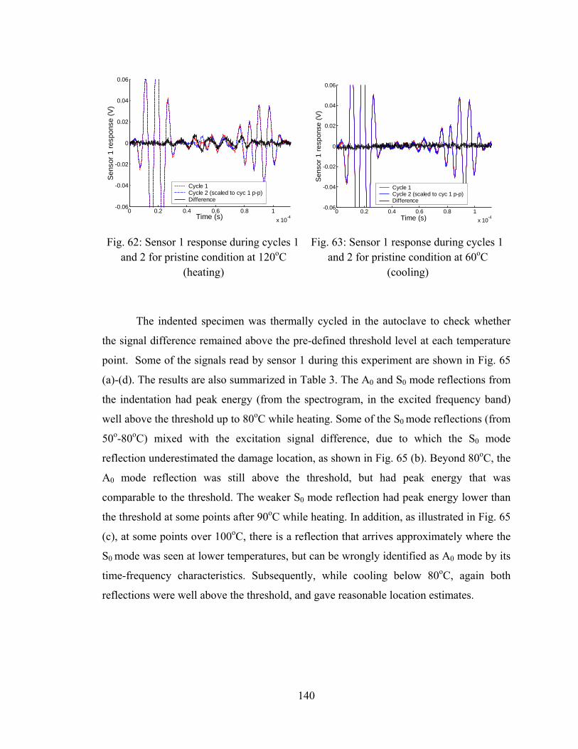
140
The indented specimen was thermally cycled in the autoclave to check whether
the signal difference remained above the pre-defined threshold level at each temperature
point. Some of the signals read by sensor 1 during this experiment are shown in Fig. 65
(a)-(d). The results are also summarized in Table 3. The A0 and S0 mode reflections from
the indentation had peak energy (from the spectrogram, in the excited frequency band)
well above the threshold up to 80oC while heating. Some of the S0 mode reflections (from
50o-80oC) mixed with the excitation signal difference, due to which the S0 mode
reflection underestimated the damage location, as shown in Fig. 65 (b). Beyond 80oC, the
A0 mode reflection was still above the threshold, but had peak energy that was
comparable to the threshold. The weaker S0 mode reflection had peak energy lower than
the threshold at some points after 90oC while heating. In addition, as illustrated in Fig. 65
(c), at some points over 100oC, there is a reflection that arrives approximately where the
S0 mode was seen at lower temperatures, but can be wrongly identified as A0 mode by its
time-frequency characteristics. Subsequently, while cooling below 80oC, again both
reflections were well above the threshold, and gave reasonable location estimates.
0 0.2 0.4 0.6 0.8 1x 10⁻⁴
-0.06
-0.04
-0.02
0
0.02
0.04
0.06
Time (s)
Sen
sor 1
resp
onse
(V)
Cycle 1Cycle 2 (scaled to cyc 1 p-p)Difference
0 0.2 0.4 0.6 0.8 1x 10⁻⁴
-0.06
-0.04
-0.02
0
0.02
0.04
0.06
Time (s)
Sen
sor 1
resp
onse
(V)
Cycle 1Cycle 2 (scaled to cyc 1 p-p)Difference
Fig. 62: Sensor 1 response during cycles 1 and 2 for pristine condition at 120oC
(heating)
Fig. 63: Sensor 1 response during cycles 1 and 2 for pristine condition at 60oC
(cooling)

141
(a) (b)
Fig. 64: Photographs of damage introduced: (a) indentation and (b) through-hole.
0 0.2 0.4 0.6 0.8 1x 10⁻⁴
-0.06
-0.04
-0.02
0
0.02
0.04
0.06
Time (s)
Sen
sor 1
resp
onse
(V)
PristineIndentationDifference
S0 mode reflection
A0 mode reflection
0 0.2 0.4 0.6 0.8 1x 10⁻⁴
-0.06
-0.04
-0.02
0
0.02
0.04
0.06
Time (s)
Sen
sor 1
resp
onse
(V)
PristineIndentationDifference
S0 mode mixed with excitation signal difference
A0 mode reflection
(a) (b)
0 0.2 0.4 0.6 0.8 1x 10⁻⁴
-0.06
-0.04
-0.02
0
0.02
0.04
0.06
Time (s)
Sen
sor 1
resp
onse
(V)
PristineIndentationDifference
S0 mode
A0 mode reflection mixed with boundary reflection difference
0 0.2 0.4 0.6 0.8 1x 10⁻⁴
-0.06
-0.04
-0.02
0
0.02
0.04
0.06
Time (s)
Sen
sor 1
resp
onse
(V)
PristineIndentationDifference
S0 mode “appears like” A0 mode
Negligible A0mode reflection
(d) (c)
Fig. 65: Sensor 1 response for pristine and indented specimens, along with the signal difference at: (a) 20oC (before thermal cycle) ; (b) 60oC while heating; (c) 140oC while
heating and (d) 40oC while cooling
142
Following this, a through hole of diameter 7.5 mm was drilled at the same
location, seen in Fig. 64 (b). The response of sensor 1 recorded after drilling through at
20oC is shown in Fig. 66 (a). The S0 mode reflection is now much stronger, while the A0
mode reflection appears much weaker (but still well above the threshold at 20oC). The
radial location estimates are 8.6 cm and 8.3 cm based on the S0 and A0 mode reflections
respectively at 20oC. The results from thermally cycling the specimen with the through-
hole are shown in Fig. 66 (a)-(d), and tabulated in Table 4. In this case, the S0 mode
reflection is reasonably above the threshold at all temperatures. There is an error of 1.9
cm in the estimate (based on the S0 mode) at 150oC, where the signal is the weakest. At a
couple of points, the radial location of the damage is overestimated by more than 1 cm
(100oC while heating and 50oC while cooling), which is possibly due to the mixing of the
S0 mode with the difference in the reflection from sensors 2 and 3. At other temperatures,
the radial location estimates based on the S0 mode are within 1 cm. The A0 mode
reflection, which was weak at 20oC to begin with, is discernible up to 70oC while heating,
but beyond that is indistinguishable from the difference in boundary reflection until the
specimen cools back to room temperature.
Thus, for “mild” damage up to 80oC, detection was not problematic, but there was
a slightly increased error in location as temperature increased. However, beyond that
temperature, there is a definite decrease in sensitivity, as reflected in the poorer
detection/characterization capability in the indentation experiment. This can be attributed
to the higher sensitivity of the substrate elastic modulus to temperature at higher
temperatures (Fig. 56), causing greater variation in the mild reflections from sensors 2
and 3, and consequently, poorer repeatability of the baseline signals. In addition, the
sensor sensitivity (in terms of signal amplitude) drops below the value at 20oC beyond
130oC. For the thru-hole, which can be termed “moderate” damage, detection was clearly
possible at all temperatures, but at a few points (3 of a total of 29 cases), there was
inaccuracy in the location estimate (by up to 2.2 cm for damage located at 8 cm), partly
due to interference with the difference in reflection from sensors 2 and 3 (simulating
structural features in field applications). One way to reduce the error in location is to use
higher center frequencies and/or fewer number of cycles (which increases frequency
bandwidth) in the actuation signal. However, that was not feasible in the present setup

143
(which did not use amplifiers), since significant distortion was observed for such
actuation signals at higher temperatures due to increasing actuator capacitance. In
addition, in the present experimental setup, the scaling of the signals to compensate for
changing actuation level increased the signal-to-noise ratio at higher temperatures. This
indicates the need for reliable actuation signal amplification for GW SHM at elevated
temperatures.
Temp. (oC)
S0 ToF (µs)
S0 energy
(V2)
Thres. energy
(V2)
S0 over
thres.?
S0 loc. (cm)
A0 ToF (µs)
A0 energy
(V2)
A0 over
thres.?
A0 loc. (cm)
20 (h) 28.10 0.0631 0.0142 Yes 7.2 50.65 0.2883 Yes 8.2
40 (h) 28.00 0.1229 0.0025 Yes 7.2 51.20 0.3695 Yes 8.6
70 (h) 18.60 0.0739 0.0154 Yes 4.7 54.60 0.5895 Yes 9.1
110 (h) 31.20 0.1808 0.1850 NO 7.9 56.00 0.1959 Yes 9.2
130 (h) 18.60 0.066 0.0517 Yes 4.5 34.10 0.0886 Yes 4.9
150 − − 0.0275 − − 25.50 0.0839 Yes 4.0
120 (c) − − 0.0375 − − 28.60 0.1363 Yes 4.1
80 (c) 25.50 0.2688 0.0525 Yes 6.5 56.80 0.1502 Yes 9.5
50 (c) 27.50 0.0681 0.0033 Yes 7.1 55.82 0.2240 Yes 9.4
20 (c) 30.35 0.0483 0.0023 Yes 7.8 53.95 0.4228 Yes 8.8
Table 3: Summary of results showing trends in thermal experiment for damage characterization with indented specimen (Key: Temp. ≡ Temperature; (h) ≡ heating
phase; (c) ≡ cooling phase ; S0 ToF ≡ time-of-flight for S0 mode reflection from indentation; Thres. ≡ Threshold; S0 loc. ≡ radial location estimate (relative to plate center)
of damage based on S0 mode reflection).

144
To conclude, this chapter examined the issue of GW SHM using piezos under
elevated temperature conditions as expected in spacecraft internal structures. Experiments
were done to determine a bonding agent (for piezos on aluminum plates) that did not
degrade at temperatures from 20oC to 150oC. Using this bonding agent (Epotek 353ND),
results from controlled experiments done to examine changes in GW propagation and
transduction using PZT-5A piezos under quasi-statically varying temperature (also from
20oC to 150oC) were presented. Thermally sensitive variables in the experiments were
0 0.2 0.4 0.6 0.8 1x 10⁻⁴
-0.06
-0.04
-0.02
0
0.02
0.04
0.06
Time (s)
Sen
sor 1
resp
onse
(V)
PristineHoleDifference
S0 mode
Mild A0 mode
0 0.2 0.4 0.6 0.8 1x 10⁻⁴
-0.06
-0.04
-0.02
0
0.02
0.04
0.06
Time (s)
Sen
sor 1
resp
onse
(V)
PristineHoleDifference
S0 mode
A0 mode
(a) (b)
0 0.2 0.4 0.6 0.8 1x 10⁻⁴
-0.06
-0.04
-0.02
0
0.02
0.04
0.06
Time (s)
Sen
sor 1
resp
onse
(V)
PristineHoleDifference
S0 mode
A0 mode mixed with boundary reflection
0 0.2 0.4 0.6 0.8 1x 10⁻⁴
-0.06
-0.04
-0.02
0
0.02
0.04
0.06
Time (s)
Sens
or 1
resp
onse
(V)
PristineHoleDifference
S0 mode
A0 mode absent
(d) (c)
Fig. 66: Sensor 1 response for pristine and thru-hole specimens, along with the signal difference at: (a) 20oC (before thermal cycle) ; (b) 70oC while heating; (c) 150oC while
heating and (d) 50oC while cooling

145
Temp. (oC)
S0 ToF (µs)
S0 energy
(V2)
Thres. energy
(V2)
S0 over
thres.?
S0 loc. (cm)
A0 ToF (µs)
A0 energy
(V2)
A0 over
thres.?
A0 loc. (cm)
20 (h) 33.45 0.2198 0.0142 Yes 8.6 49.75 0.0763 Yes 8.3
40 (h) 34.30 0.2972 0.0025 Yes 8.8 55.20 0.1119 Yes 9.0
70 (h) 32.50 0.2463 0.0154 Yes 8.3 56.70 0.2128 Yes 9.0
110 (h) 40.60 0.2578 0.1850 Yes 10.2 Bndry − − −
130 (h) 33.40 0.3105 0.0517 Yes 8.2 Bndry − − −
150 25.60 0.1073 0.0275 Yes 6.1 Bndry − − −
120 (c) 31.00 0.1997 0.0375 Yes 7.6 Bndry − − −
80 (c) 28.00 0.2985 0.0525 Yes 7.0 Bndry − − −
50 (c) 36.20 0.3393 0.0033 Yes 9.3 Bndry − − −
20 (c) 33.80 0.2018 0.0023 Yes 8.7 53.60 0.0623 Yes 8.8
Table 4: Summary of results showing trends in thermal experiment for damage characterization using specimen with thru-hole (Key: Temp. ≡ Temperature; (h) ≡
heating phase; (c) ≡ cooling phase; S0 ToF ≡ time-of-flight for S0 mode reflection from thru-hole; Thres. ≡ Threshold; S0 loc. ≡ radial location estimate (relative to plate center)
of damage based on S0 mode reflection; Bndry ≡ A0 mode reflection peak within boundary reflection).
identified and quantified to model the experimentally observed changes under
temperature variation. The increase in time-of-flight of GW pulses with increasing
temperature was captured by the model (within the error margins). However, there was a
significant gap in the prediction of the large increase in sensor response amplitude up to
100oC. The stronger vulnerability of pitch-catch approaches to false positives under
changing temperature was then explained. Finally, detection and location of damage (by
drilling) using the pulse-echo approach in the presence of mild structural GW scatterers
(to simulate rivets) was explored in the same temperature range. Damage characterization

146
of a half-plate thickness indentation at 8 cm from the actuators was not significantly
affected up to 80oC, but beyond that temperature, detection/characterization was difficult.
The problems beyond 80oC can be traced to increased sensitivity of substrate elastic
modulus to temperature and weaker sensor sensitivity beyond 130oC. For a through-hole,
damage detection and characterization was possible at all temperatures and except at a
few temperatures (3 out of 29), damage was located within 1 cm for a nominal location of
8 cm and hole diameter 0.75 cm. Suggested approaches for improving sensitivity at
higher temperatures include testing at higher frequencies and/or with shorter time-span
excitation pulses, with reliable actuation amplifiers.

147
CHAPTER VI
GUIDED-WAVE EXCITATION BY PIEZOS IN
COMPOSITE LAMINATED PLATES
The studies till this point in the thesis have focused on isotropic structures. With
composite materials becoming increasingly common in aerospace structures as explained
in Section I.1, there is a need to extend that work to composite structures as well. The
present chapter seeks to extend the modeling work in Chapter II for GW excitation by
finite-dimensional piezos to multilayered, laminated fiber-reinforced composite plates.
Details of the implementation of the formulation and verification of the models using
numerical simulations are also presented.
VI. 1 Theoretical Formulation
As in Chapter II, first a general expression for the GW field excited by an
arbitrary shape piezo-actuator surface-bonded on a multilayered composite plate is
derived. Consider an infinite N-layered composite plate of total thickness H, with such an
actuator bonded on one free surface, as illustrated in Fig. 67. The origin is located on the
free surface with the actuator and the X3-axis is normal to the plate surface. The
individual layers are assumed to have unidirectional fibers in a matrix and are modeled as
being transversely isotropic with uniform density. This is a reasonable assumption if the
GW wavelength is large compared to the inter-fiber spacing and the fiber diameter [62].
The solution procedure consists of the following four components (illustrated in Fig. 68):
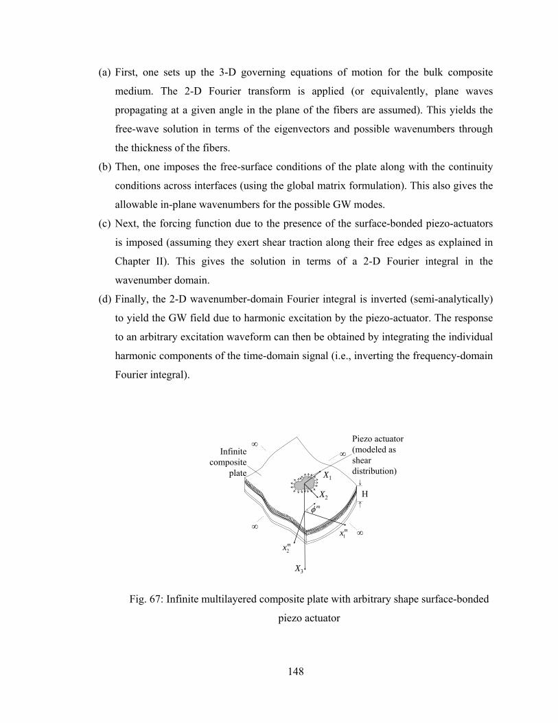
148
(a) First, one sets up the 3-D governing equations of motion for the bulk composite
medium. The 2-D Fourier transform is applied (or equivalently, plane waves
propagating at a given angle in the plane of the fibers are assumed). This yields the
free-wave solution in terms of the eigenvectors and possible wavenumbers through
the thickness of the fibers.
(b) Then, one imposes the free-surface conditions of the plate along with the continuity
conditions across interfaces (using the global matrix formulation). This also gives the
allowable in-plane wavenumbers for the possible GW modes.
(c) Next, the forcing function due to the presence of the surface-bonded piezo-actuators
is imposed (assuming they exert shear traction along their free edges as explained in
Chapter II). This gives the solution in terms of a 2-D Fourier integral in the
wavenumber domain.
(d) Finally, the 2-D wavenumber-domain Fourier integral is inverted (semi-analytically)
to yield the GW field due to harmonic excitation by the piezo-actuator. The response
to an arbitrary excitation waveform can then be obtained by integrating the individual
harmonic components of the time-domain signal (i.e., inverting the frequency-domain
Fourier integral).
Infinite composite
plate
Piezo actuator (modeled as shear distribution)
∞
∞
∞
∞
X2
X1
H
X3
2mx
1mx
mφ
Fig. 67: Infinite multilayered composite plate with arbitrary shape surface-bonded
piezo actuator

149
Among these, parts (a) and (b) are adapted from Auld [10] and Lih and Mal [62]. Parts
(c) and (d) are based on the work in Chapter II. The details of the solution procedure are
explained in the following sub-sections.
VI. 1.A Bulk Waves in Fiber-reinforced Composites
First, consider the general solution for bulk waves in a transversely isotropic
medium. The equations of motion for the bulk medium in each layer are:
T ρ=c u u∇ ∇ (120)
where u is the “local” displacement vector (later the “global” displacement vector u will
be introduced for the laminate), c is the stiffness matrix, the ⋅ over a variable indicates
derivative with respect to time, ρ is the material density, and the operator ∇ is defined
as:
∞
∞
∞
∞∞∞
∞
∞ ∞
∞
O1K 2K
K → ∞
C
1K−2K− RK
IK
(a) Plane wave solution for infinite bulk composite [10]
(b) Free GW solution for infinite multi-layered composite plate [61]
(c) Forcing function due to surface-bonded piezo (shear traction along edge)
(d) Wavenumber Fourier integral inversion (residue calculus)
x1
x3
x2
X1
X3
X2
Fig. 68: Illustration of solution procedure

150
1 3 2
2 3 1
3 2 1
0 0 0
0 0 0
0 0 0
x x x
x x x
x x x
⎡ ⎤∂ ∂ ∂⎢ ⎥∂ ∂ ∂⎢ ⎥⎢ ⎥∂ ∂ ∂
= ⎢ ⎥∂ ∂ ∂⎢ ⎥⎢ ⎥∂ ∂ ∂⎢ ⎥
∂ ∂ ∂⎣ ⎦
∇ (121)
If the fibers are oriented along the 1-direction in the local coordinate system (x1, x2, x3) of
the material, the stress-strain relation and the stiffness matrix c for a transversely
isotropic material are:
1,1 11 12 1211
2,2 12 22 2322
3,3 12 23 223344
2,3 3,2 4423
1,3 3,1 5531
2,1 1,2 5512
0 0 00 0 00 0 0
; , with 0 0 0 0 00 0 0 0 00 0 0 0 0
u c c cu c c cu c c c cc
u u cu u cu u c
σσσσσσ
⎡ ⎤ ⎡ ⎤⎡ ⎤⎢ ⎥ ⎢ ⎥⎢ ⎥⎢ ⎥ ⎢ ⎥⎢ ⎥⎢ ⎥ ⎢ ⎥⎢ ⎥
= = =⎢ ⎥ ⎢ ⎥⎢ ⎥ +⎢ ⎥ ⎢ ⎥⎢ ⎥⎢ ⎥ ⎢ ⎥⎢ ⎥ +⎢ ⎥ ⎢ ⎥⎢ ⎥
+⎢ ⎥ ⎢ ⎥⎢ ⎥⎣ ⎦ ⎣ ⎦⎣ ⎦
c c 22 23
2c− (122)
Here ijσ , with i and j taking integer values from 1 to 3, are the local stress components.
Next, constants are introduced that correspond to the squares of the bulk wave speeds
along the principal directions:
1 22
2 11
3 12 55
4 22 23 44
/ (dilatational wave normal to the fiber direction)/ (dilatational wave along the fiber direction)
( ) / (shear wave in the plane of isotropy) ( ) / 2 / (shear wav
a ca ca c ca c c c
ρρ
ρρ ρ
=== += − =
5 55
e along the fiber direction) / (shear wave in the plane of isotropy)a c ρ=
(123)
Viscoelastic damping can be modeled by the use of complex stiffness constants. Suppose
the wavenumber components are ξ1, ξ2 and ζ along the 1-, 2- and 3- local directions,
respectively. Furthermore, without loss of generality, consider harmonic excitation at
angular frequency ω. Then the wave field is of the form:
( )1 1 2 2 3i x x x te ξ ξ ζ ω− + + −=u Ω (124)

151
where the vector Ω is a linear superposition of the possible eigenvectors. To solve for
these eigenvectors, from Eqs. (120)-(124), one obtains the Christoffel equation:
2 2 211 1 55 2 12 55 1 2 12 55 1 1 1
2 2 2 212 55 1 2 55 1 22 2 44 23 44 2 2 2
2 2 212 55 1 23 44 2 55 1 44 2 22 3 3
( ) ( ) ( )( ) ( )( ) ( )
c c c c c cc c c c c c cc c c c c c c
ξ ξ ζ ξ ξ ξ ζξ ξ ξ ξ ζ ξ ζ ρωξ ζ ξ ζ ξ ξ ζ
⎡ ⎤ ⎡ ⎤ ⎡ ⎤+ + + + Ω Ω⎢ ⎥ ⎢ ⎥ ⎢ ⎥+ + + + Ω = Ω⎢ ⎥ ⎢ ⎥ ⎢ ⎥⎢ ⎥ ⎢ ⎥ ⎢ ⎥+ + + + Ω Ω⎣ ⎦ ⎣ ⎦⎣ ⎦
(125)
For fixed values of ξ1, ξ2, and ω, there are six possible roots ±ζi, i = 1 to 3, of this
equation. The first two pairs of roots correspond to pairs of quasi-longitudinal waves
(characterized by displacements dominantly along the wave propagation direction but
with small components normal to it) and quasi-shear waves (characterized by
displacements dominantly normal to the wave propagation direction but with small
components along it, see [10]). The wavenumbers in the thickness direction for these four
roots are, respectively [62]:
2 2 2 21 2 1 2 2 2
2 2
1 2
2 2 2 2 2 2 2 21 5 1 2 5 3 1 1 5 2 1 5 1
;
; 2 2 2 2
; =( ) ( ); =( )( )
b b
b b
a a a a a a a a a a
ζ ξ ζ ξ
β β γ β β γα α α α α α
α β ξ ω γ ξ ω ξ ω
= − + = − +
⎛ ⎞ ⎛ ⎞ ⎛ ⎞ ⎛ ⎞= − − − = − + −⎜ ⎟ ⎜ ⎟ ⎜ ⎟ ⎜ ⎟⎝ ⎠ ⎝ ⎠ ⎝ ⎠ ⎝ ⎠
= + − − + − −
(126)
The third pair of roots corresponds to quasi-shear waves and their through-thickness
wavenumbers are given by:
2 2 2 23 2 5 1 4( ) /a aζ ξ ω ξ= − + − (127)
The displacement eigenvectors resulting from Eq. (125) corresponding to these roots are:
[ ][ ][ ]
1 1 11 2 21 1 21
2 1 12 2 22 2 22
3 3 20
T
T
T
i q i q i q
i q i q i q
i i
ξ ξ ζ
ξ ξ ζ
ζ ξ
=
=
= −
e
e
e
(128)
where:
2 211 3 1 21 2 1 5 1
2 221 3 2 22 2 1 5 2
;
;
q a b q a a b
q a b q a a b
ω ξ
ω ξ
= = − −
= = − − (129)

152
and the other three eigenvectors e4, e5 and e6 are obtained by replacing ζi by −ζi. The
general solution for the displacement vector is then given by:
[ ]
1 3 2 3 3 3
1 1 2 2
1 3 2 3 3 3
1 1 2 2
1 1 2 2 3 3 ( )
1 4 2 5 3 6
( )311 12
3
( ) 00 ( )
i x i x i xi x x t
i x i x i x
i x x t
C e C e C ee
C e C e C e
xe
x
ζ ζ ζξ ξ ω
ζ ζ ζ
ξ ξ ω
+ + + − + −
− − −− − −
+ − + −+
−−
⎛ ⎞+ + +⎜ ⎟⎜ ⎟+ + +⎝ ⎠
⎡ ⎤ ⎡ ⎤= ⎢ ⎥ ⎢ ⎥
⎣ ⎦⎣ ⎦
e e eu =
e e e
CEQ Q
CE
(130)
where Ci±, i = 1 to 3, are free constants and:
[ ] [ ]1 3 2 3 3 3
1 3 2 3 3 3
11 1 2 3 12 4 5 6
3
3
;
( ) Diag , ,
( ) Diag , ,
i x i x i x
i x i x i x
x e e e
x e e e
ζ ζ ζ
ζ ζ ζ−
= =
⎡ ⎤= ⎣ ⎦⎡ ⎤= ⎣ ⎦
+
Q e e e Q e e e
E
E
(131)
VI. 1.B Assembling the Laminate Global Matrix from the Individual Layer Matrices
With the general solution for the bulk medium in place, one can then seek the
particular solution for the problem at hand. As mentioned earlier, the equations in this
particular sub-section are adapted from Lih and Mal [62].
Due to the different orientations of the fibers in the different layers, it is useful to
work with a global coordinate system (X1, X2, X3) distinct from the local coordinate
system, for which the 1mx -axis is aligned with the fiber direction (with the superscript m
indicating the layer number between 1 and N). However, the X3- and 3mx -axes are
coincident and the two coordinate systems differ only in the plane of the plate. One can
relate the displacement vector u in the global system and u in the local system using the
transformation matrix Lm (defining φm to be the angle between the X1- and 1mx -axes):
cos sin 0; where sin cos 0
0 0 1
m m
m m m m m
φ φφ φ
⎡ ⎤−⎢ ⎥= ⎢ ⎥⎢ ⎥⎣ ⎦
u = L u L (132)
The surface traction conditions for this problem are:
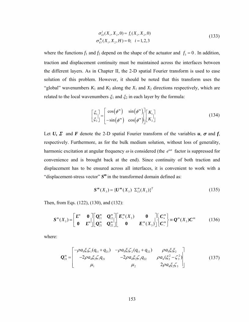
153
13 1 2 1 2
3 1 2
( , ,0) ( , ,0)
( , , ) 0; 1, 2,3iX X f X X
X X H i
σ
σ
=
= =i
Ni
(133)
where the functions f1 and f2 depend on the shape of the actuator and 3 0f = . In addition,
traction and displacement continuity must be maintained across the interfaces between
the different layers. As in Chapter II, the 2-D spatial Fourier transform is used to ease
solution of this problem. However, it should be noted that this transform uses the
“global” wavenumbers K1 and K2 along the X1 and X2 directions respectively, which are
related to the local wavenumbers ξ1 and ξ2 in each layer by the formula:
( ) ( )( ) ( )
1 1
2 2
cos sin
sin cos
m m
m m
KK
φ φξξ φ φ
⎡ ⎤⎡ ⎤ ⎡ ⎤⎢ ⎥=⎢ ⎥ ⎢ ⎥⎢ ⎥−⎣ ⎦ ⎣ ⎦⎣ ⎦
(134)
Let U, Σ and F denote the 2-D spatial Fourier transform of the variables u, σ and f,
respectively. Furthermore, as for the bulk medium solution, without loss of generality,
harmonic excitation at angular frequency ω is considered (the i te ω factor is suppressed for
convenience and is brought back at the end). Since continuity of both traction and
displacement has to be ensured across all interfaces, it is convenient to work with a
“displacement-stress vector” Sm in the transformed domain defined as:
3 3 3 3( ) ( ) ( )m TiX X X= Σm mS U (135)
Then, from Eqs. (122), (130), and (132):
311 123 3
321 22
( )( ) ( )
( )
mm mm mm m m
mm m mm
XX X
X −
⎡ ⎤⎡ ⎤ ⎧ ⎫⎡ ⎤= ≡⎨ ⎬⎢ ⎥⎢ ⎥⎢ ⎥
⎣ ⎦ ⎣ ⎦ ⎩ ⎭⎣ ⎦
0000
+ +
-
EQ QL CS Q CEQ Q CL
(136)
where:
5 1 1 11 21 5 1 2 11 22 5 1 22 2
21 4 2 1 21 4 2 2 22 4 2 3
1 2 4 2 3
( ) ( )2 2 ( )
2
m
a q q a q q aa q a q a
a
ρ ξ ζ ρ ξ ζ ρ ξ ξρ ξ ζ ρ ξ ζ ρ ξ ζ
µ µ ρ ξ ζ
− + − +⎡ ⎤⎢ ⎥= − − −⎢ ⎥⎢ ⎥⎣ ⎦
Q (137)

154
5 1 1 11 21 5 1 2 11 22 5 1 22 2
22 4 2 1 21 4 2 2 22 4 2 3
1 2 4 2 3
2 2 21 5 3 1 11 1 4 2 21 1 1 21
2 2 22 5 3 1 12 1 4 2 22 1 1 2
( ) ( )2 2 ( )
2
( ) ( 2 )
( ) ( 2 )
m
Tm m m
a q q a q q aa q a q a
a
a a q a a q a q
a a q a a q a q
ρ ξ ζ ρ ξ ζ ρ ξ ξρ ξ ζ ρ ξ ζ ρ ξ ζ
µ µ ρ ξ ζ
µ ρ ξ ξ ζ
µ ρ ξ ξ ζ
+ −
+ +⎡ ⎤⎢ ⎥= −⎢ ⎥⎢ ⎥−⎣ ⎦
⎡ ⎤= ⎣ ⎦⎡ ⎤= − − − −⎣ ⎦
= − − − −
Q
C C C
1 1 11 3 3 2 3 3 3 3 3
1 3 3 2 3 3 3 3 3
2
( ) ( ) ( )3
( ) ( ) ( )3
( ) Diag , ,
( ) Diag , ,
m m m
m m m
i X X i X X i X Xm
i X X i X X i X Xm
X e e e
X e e e
ζ ζ ζ
ζ ζ ζ
− − −− − −+
− − −−
⎡ ⎤⎣ ⎦⎡ ⎤= ⎣ ⎦⎡ ⎤= ⎣ ⎦
E
E
(138)
with 3mX being the X3-coordinate of the interface between layers m and (m−1). Here 21
mQ
and 22mQ are matrices whose columns are the stress eigenvectors for the mth layer
corresponding to wavenumbers along the 3-axis, ζi and −ζi, respectively. These are
obtained from the displacement eigenvectors using Eq. (121). The interface continuity
conditions can then be expressed as:
1 1
1 1 1 13 3
where ( ); ( )
m m m m
m m m m m mX X
+ ++ −
+ + + ++ −
= −
≡ ≡
Q C Q C
Q Q Q Q (139)
These equations ensure continuity of all displacement and traction components at the
interface across two layers. The surface traction conditions can be expressed as:
1 1
1 1 1 1 1 121 22 21 22
ˆ ˆ ;ˆ ˆwhere ;
N N
N N N N N N
− − + +
− +
= =
⎡ ⎤ ⎡ ⎤= − − =⎣ ⎦ ⎣ ⎦
0Q C F Q C
Q LQ LQ E Q L Q E L Q (140)
Here the matrices Q correspond to the lower-half of Q relating to stress. The system of
equations is then solved by assembling Eqs. (139) and (140) together into a 6N × 6N
banded matrix (called the global matrix, say G):

155
1 1
1 2 2
1
1
1
ˆ
ˆ
m m
m m
N N
NN
−
+ −
−+ −
++ −
−+ −
+
⎡ ⎤ ⎡ ⎤ ⎡ ⎤⎢ ⎥ ⎢ ⎥ ⎢ ⎥⎢ ⎥ ⎢ ⎥ ⎢ ⎥⎢ ⎥ ⎢ ⎥ ⎢ ⎥⎢ ⎥ ⎢ ⎥ ⎢ ⎥⎢ ⎥ ⎢ ⎥ ⎢ ⎥=⎢ ⎥ ⎢ ⎥ ⎢ ⎥⎢ ⎥ ⎢ ⎥ ⎢ ⎥⎢ ⎥ ⎢ ⎥ ⎢ ⎥⎢ ⎥ ⎢ ⎥ ⎢ ⎥⎢ ⎥ ⎢ ⎥ ⎢ ⎥⎢ ⎥ ⎢ ⎥ ⎢ ⎥⎣ ⎦⎣ ⎦⎣ ⎦
00 0
0 00 0
000
Q FCQ Q C
Q QQ Q
Q QCQ
(141)
Alternatively, if the layup is symmetric about the mid-plane of the plate, then the
system can be solved for the symmetric and anti-symmetric modes separately, thereby
saving some computational time. The surface condition must also be split into its
“symmetric” and “anti-symmetric” components. Then, the relevant surface condition on
the top layer is enforced along with the continuity conditions up to the interface between
layers 2N and 2 1N − along with conditions of symmetry (u3, σ32 and σ31 being zero at
the mid-plane) or anti-symmetry (u1, u2 and σ33 being zero at the mid-plane). The
problem is thus reduced to two systems, each of complexity 3N × 3N. With the problem
constraints now enforced, if the forcing function is also known, this equation can be
solved to find the constants, Cm.
VI. 1.C Forcing Function due to Piezo-actuator
The piezo actuator is modeled as causing in-plane shear traction of uniform
magnitude (say τ0 per unit length) along its perimeter, in the direction normal to the free
edge on the plate surface X3 = 0 (see Fig. 68), as was done in Chapter II. While the above
formulation is generic enough to capture GW excitation by an arbitrary shape piezo, for
brevity only the rectangular piezo shape is analyzed here. For the rectangular uniformly
poled piezo-actuator of dimensions 2A1 × 2A2 (along the X1- and X2-axes respectively),
which is located at the center of the coordinate system:

156
( )( )
( )( )
1 0 1 1 1 1 2 2 2 2
1 0 1 1 2 2 2
2 0 1 1 1 1 2 2 2 2
2 0 1 1 2 2 1
3 3
( ) ( ) ( ) ( )4 sin( )sin( ) /
( ) ( ) ( ) ( )4 sin( )sin( ) /
0; 0
f X A X A He X A He X AF K A K A iKf He X A He X A X A X AF K A K A iKf F
τ δ δτ
τ δ δτ
= − − + + − −
= −
= + − − − − +
= −= =
(142)
where He( ) is the Heaviside function. The constants in Eq. (141) can then be analytically
solved using Cramer’s rule:
111
2
11
1
1
( , ) , etc.,( , )
where ( , ) det
ˆ
( , ) det( )
m m
m m
N N
N
N KCK
N K
K
+
+
−− +
+− +
−− +
−
Γ=
∆ Γ
⎡ ⎤⎢ ⎥⎢ ⎥⎢ ⎥⎢ ⎥⎢ ⎥Γ = ⎢ ⎥⎢ ⎥⎢ ⎥⎢ ⎥⎢ ⎥⎢ ⎥⎣ ⎦
∆ Γ =
00 0
0 00 0
0
0 0
FQ
Q QQ Q
Q Q
QG
(143)
where K and Γ are the polar wavenumber coordinates, related to the Cartesian ones by the
formulas:
( ) ( )2 2 -11 2 2 1; tanK K K K K= + Γ = (144)
VI. 1.D Spatial Fourier Integral Inversion
With the constants known, the expression for displacement in the wavenumber domain
can be obtained from Eqs. (136) and (143). Fourier inversion can then be used to recover
the spatial domain solution. For the case of a rectangular actuator, this leads to an
expression of the following form for displacement along the 1-direction in the spatial
domain:

157
1 2
02 1 22
1 3( ( cos sin ) )0 0
sin( cos )sin( sin )( 0)
( , )( , )
i K X X t
KA KAiu X KdKd
N K eK
π
ω
τπ∞
− Γ+ Γ −
−⎛ ⎞Γ Γ⎜ ⎟⎜ ⎟= = Γ
Γ⎜ ⎟×⎜ ⎟∆ Γ⎝ ⎠
∫ ∫
(145)
The procedure for inversion of this integral is analogous to that in Section II.4. The
integrand is singular at the roots ˆ ( )K Γ of ( , ) 0K∆ Γ = , which is the dispersion equation
for the multilayered composite plate. These roots are the allowable in-plane radial
wavenumbers for the multilayered composite plate at angular frequency ω. ( , )K∆ Γ is
symmetric about the K-axis. The final expression for u1 that would be obtained is:
1
1 1
1
2
2 2
2
3
3 3
3
2ˆ( cos( ) )0
1 3ˆ
2
2ˆ( cos( ) )0
ˆ2
2ˆ( cos( ) )0
ˆ2
ˆ( , )( 0) . ˆ4 ( , )
ˆ( , ). ˆ4 ( , )
ˆ( , ). ˆ4 ( , )
i KR t
K
i KR t
K
i KR t
K
N Ku X e dK
N K e dK
N K e dK
π
ω
π
π
ω
π
π
ω
π
τπ
τπ
τ τπ
Θ +
− Γ−Θ −
Θ −
Θ +
− Γ−Θ −
Θ −
Θ +
− Γ−Θ −
Θ −
− Γ= = Γ +
′∆ Γ
Γ+ Γ +
′∆ Γ
−Γ+ Γ +
′∆ Γ
∑ ∫
∑ ∫
∑ ∫4
4 4
4
2ˆ( cos( ) )0
ˆ2
ˆ( , ). ˆ4 ( , )i KR t
K
N K eK
π
ω
π π
Θ +
− Γ−Θ −
Θ −
Γ′∆ Γ
∑ ∫
(146)
where:
( ) ( )2 21 2 21 1 1 1 2 2
1 1
tan ; , etc.X A R X A X AX A
− ⎛ ⎞−Θ = = − + −⎜ ⎟−⎝ ⎠
(147)
Again, this notation is analogous to that in Section II.4. Furthermore, an approximate
closed form solution can be obtained for the far field using the method of stationary
phase. This is assuming damping is not modeled and that the integrand is real-valued. If
damping is modeled, then a similar approximation can be done using the method of
steepest descent [11]. Thus, for large values of R (which leads to large values of
, 1 to 4kR k = ):

158
1 1 1
1
2 2 2
2
ˆ( cos( ) )0 1 41 3 2ˆ 11
1 2
ˆ( cos( ) )0 2 42ˆ 22
2 2
23
3 2
ˆ( , )2( 0) ˆˆ 4 ( , )( cos( )).
ˆ( , )2ˆˆ 4 ( , )( cos( )).
2ˆ( cos( )).
i KR t
K
i KR t
K
N Ku X eKd KR
d
N K eKd KR
d
d KRd
πω
πω
τππ
τππ
π
− Γ −Θ − +
Γ=Γ
− Γ −Θ − +
Γ=Γ
Γ
− Γ= = +
′∆ ΓΓ − ΘΓ
Γ+ +
′∆ ΓΓ − ΘΓ
+Γ − Θ
Γ
∑
∑
3 3 3
3
4 4 4
4
ˆ( cos( ) )0 3 4
ˆ 3
ˆ( cos( ) )0 4 42ˆ 44
4 2
ˆ( , )ˆ4 ( , )
ˆ( , )2ˆˆ 4 ( , )( cos( )).
i KR t
K
i KR t
K
N K eK
N K eKd KR
d
πω
πω
τπ
τππ
− Γ −Θ − +
=Γ
− Γ −Θ − +
Γ=Γ
Γ+
′∆ Γ
− Γ+
′∆ ΓΓ − ΘΓ
∑
∑
(148)
where ˆ1tan( ) ˆk k
dKdK
Γ − Θ =Γ
. Thus, ( )k kΓ −Θ is the angle between the phase velocity
and group velocity vectors [10], as shown in Fig. 69 (a). For composites, the group
velocity is along the normal to the “slowness curve,” which is the polar plot of the
reciprocal of the phase velocity versus propagation direction. This implies that the
contributions from kΓ dominate the integrals over Γ at large distances from the source.
This reiterates a well-known fact about wave propagation in anisotropic media, i.e., the
wave travels at a “steering angle,” which may be different from the angle that it was
launched along by its source [10], as shown in Fig. 69 (b).
VI. 2 Implementation of the Formulation and Slowness Curve Computation
The theoretical formulation described above was implemented in Fortran 90. The
linear algebra package LAPACK [229] for Fortran 90 was employed to evaluate the
determinants of large banded matrices. The roots of the dispersion equation ( , ) 0K∆ Γ = were simply computed by the “zero-crossing” approach, i.e., by evaluating the
determinant of the matrix over a fine grid in the (K,Γ) plane and looking for sign changes

159
in the value of the determinant. In doing so, one has to avoid the bulk wave velocities of
the composite material, which are also roots of the dispersion equation. One also has to
take care to use double-precision variables and compute the roots with high precision
since with the very large matrices involved, small errors in the values of the roots cause
large errors in the response solution. Furthermore, in tracking zero-crossings on a grid of
( , )K Γ , due to the large variations in order of magnitude, it is convenient to plot
determinant values on a logarithmic scale. The derivatives w.r.t. K were evaluated
analytically. The code implemented in Fortran 90 to evaluate the determinant values (for
zero-crossings) and integrand values (for the kernel of the integral) was computationally
efficient, with each run being completed in a few minutes on a standard desktop
computer (1.2 GHz Pentium IV with 256 MB RAM). The integrals over Γ were evaluated
numerically (by summing the integrand’s values taken at intervals of 1o).
Some results for the slowness curves obtained are presented here. Graphite-epoxy
composite plates (material properties: ρ = 1578 kg/m3; c11 = 160.73 GPa, c12 = 6.44 GPa,
c22 = 13.92 GPa, c23 = 6.92 GPa, c55 = 7.07 GPa; this is the same material used in [62])
were analyzed. Damping was not considered for these analyses. The slowness surfaces
Slowness curve
Kω
2Kω
1Kω
kΓ
(det )( )(det )
Kgr ω
∇Γ =
∂ ∂Gc
G
( ) 1ˆ1tan ˆk k
dKdK
− ⎛ ⎞Γ − Θ = ⎜ ⎟
Γ⎝ ⎠
det ( , , ) 0Kω Γ =G
GW pulse
Actuator
Sensor
cph
cgr
Anisotropic solid
(a) (b)
Fig. 69: (a) Relation between group velocity and slowness curve and (b) “Steering” in
anisotropic media

160
(plots of inverse of phase velocity versus propagation direction) for the A0 and S0 modes
in a 1-mm thick unidirectional plate at 500 kHz are shown in Fig. 70 (a). As seen there,
the wavespeeds along the fiber direction (0o) are much faster than those along the normal
direction. The corresponding plots for a quasi-isotropic laminate at 200 kHz of layup
[0/45/-45/90]s, with each ply being 0.11 mm thick, is shown in Fig. 70 (b). The S0 mode
for this laminate is approximately isotropic, with the differences in wavespeeds along
different directions being invisible to the naked eye. However, the A0 mode for the same
laminate has significant directional dependence.
VI. 3 Results and Comparison with Numerical Simulations
Results were generated for a couple of test cases to compare with FEM
simulations using ABAQUS [205] and examine the correlation between the two in terms
of angular dependence of GW radiation patterns. The cases examined were for the
unidirectional (in antisymmetric mode) and quasi-isotropic composite plates (in
symmetric mode) described above, for which slowness curves were generated. In the case
of the unidirectional plate, due to symmetry about three axes, a 1/8th plate section of size
0.0002 0.0004
0.0006
0.0008
0.001
30
210
60
240
90
270
120
300
150
330
180 0
Angle (degrees)
Slo
wne
ss (s
/m)
A0 modeS0 mode0
0
0.0005
0.001
0.0015
30
210
60
240
90
270
120
300
150
330
180 0
Angle (degrees)
Slo
wne
ss (s
/m)
A modeS mode
00
(a) (b)
Fig. 70: Slowness curves for (a) 1-mm unidirectional plate at 500 kHz and (b) quasi-
isotropic laminate at 200 kHz of layup [0/45/-45/90]s, each ply being 0.11-mm thick

161
3 cm × 3 cm × 0.5 mm was modeled. For the quasi-isotropic plate, since it is symmetric
about only one axis, a half-plate section of the modeled area was 20 cm × 20 cm × 0.44
mm (illustrated in Fig. 76). The quasi-isotropic plate also has “periodic” symmetry in the
plane of the plate, i.e., the half-section from 0o to 180o can be rotated about an axis going
through the plate center normal to its plane by 180o to obtain the other half. However, this
cannot be used to reduce problem complexity in ABAQUS. A uniform mesh of 3-D 8-
noded brick elements was used and the elements were small enough (0.375 × 0.375 ×
0.125 mm3 for the unidirectional plate and 1.3 × 1.3 × 0.11 mm3 for the quasi-isotropic
laminate) to resolve the smallest wavelength excited over the frequency bandwidth. The
element edges were all parallel to any of the three coordinate axes shown. Infinite
elements could not be used to suppress reflections in these simulations, since they are not
available in ABAQUS for use with anisotropic materials. Therefore, the simulation
results were only used till the first excited GW pulse hit the plate boundary. Transversely
isotropic material properties (identical to the values in Section VI. 2) were specified for
the individual finite elements. For the transversely isotropic composite plate, four
separate layers were modeled using one layer of finite elements each, and different
material orientations were specified to model the [0/45/-45/90]s layup. Symmetry
conditions were imposed along two edges along the in-plane axes for the unidirectional
composite. Since antisymmetric modes were of interest for the unidirectional composite,
thru-thickness antisymmetry conditions were applied to the nodes on the lower plate
surface. Similarly, thru-thickness symmetric conditions were applied to the nodes on the
lower plate surface of the quasi-isotropic laminate. On the upper plate surface of the
unidirectional composite, to simulate the action of a square piezo exciting GWs at the
center, a quarter section of the piezo was modeled. The complete piezo was modeled for
the quasi-isotropic laminate. Shear forces were applied at nodes along the piezo’s edges.
In both cases, a 3.5-cycle Hanning window-modulated sinusoidal toneburst with
center frequency 200 kHz was applied as excitation signal by specifying this waveform
for the time variation of the shear force applied at the piezo’s edges. Again, the time step
was chosen to be small enough to accurately capture the highest excited frequency. The
out-of-plane displacements over the plate’s top surface (which has the surface-bonded

162
piezo on it) were recorded at various time steps. The corresponding values from the semi-
analytical model were also generated. The results are shown in Fig. 72 and Fig. 73 for the
unidirectional composite and quasi-isotropic laminate respectively, both normalized to
the respective peak value of out-of-plane displacement over all time steps. Only results
from half the plate-section of the quasi-isotropic plate are shown, due to its periodic
symmetry. The row of nodes immediately adjacent to the piezo was not considered for
the normalization to avoid errors due to the local numerical noise caused by the discrete
nodal shear forces.
To generate the antisymmetric mode surface plots from the semi-analytical model
for the unidirectional composite, only the A0 mode was considered, since the highest
frequency in the excited bandwidth is below the cutoff frequency for the A1 mode.
Similarly, to generate the symmetric mode surface plots for the quasi-isotropic plate, only
the S0 mode was considered. While the SH0 mode also exists for the symmetric mode
analysis at all frequencies, being approximately isotropic, it can be considered to be a
“pure” mode [10]. Thus, the displacements in this case are for all practical purposes
xy
z
‘xsymm’ surface condition in ABAQUSon x = 0
‘ysymm’ surface condition in ABAQUSon y = 0
‘zasymm’ surface condition in ABAQUS (lower surface)
3 cm
Shear forces at nodesPiezo location
(0.15 × 0.15 cm2)
3 cm
0.5 mm
xy
z
‘zsymm’ surface condition in ABAQUS (lower surface)
Shear forces at nodes
Piezo location (1 × 1 cm2)0.44
mm
(a) (b)
Fig. 71: Geometry of FEM models for: (a) 1-mm unidirectional plate and (b) quasi-isotropic
plate of layup [0/45/-45/90]s, each ply being 0.11 mm thick.

163
1 cm
t = 8.0 µs
1 cm
t = 8.0 µs
1 cm
t = 11.2 µs
1 cm
t = 11.2 µs
1 cm
t = 14.4 µs
1 cm
t = 14.4 µs
(a) (b)
Fig. 72: Surface out-of-plane displacements at different time instants for the unidirectional
composite excited in the antisymmetric mode (by the piezo, in gray) with a 3.5-cycle
Hanning windowed toneburst at 200 kHz obtained using: (a) FEM (b) the developed model.

164
t = 11.2 µs
5 cm 5 cm
t = 11.2 µs
t = 14.4 µs
5 cm 5 cm
t = 14.4 µs
t = 17.6 µs
5 cm 5 cm
t = 17.6 µs
(a) (b)
Fig. 73: Surface out-of-plane displacements at different time instants for the quasi-isotropic
composite excited symmetrically (by the piezo, in gray) with a 3.5-cycle Hanning
windowed toneburst at 200 kHz obtained using: (a) FEM (b) the developed model.

165
within the plane of the plate. Therefore, as in the analysis for isotropic plates, it does not
cause out-of-plane displacements. However, the SH0 mode would contribute to symmetric
mode simulations for the unidirectional composite plate. This is because in that case, it is
significantly dependent on direction and is therefore a “quasi-” SH0 mode. Consequently,
the displacement patterns in this mode are not entirely in the plane of the plate for
directions not along or normal to the fiber direction.
The results from the FEM simulations are in agreement with that obtained from
the semi-analytical model, thus verifying the accuracy of the model within the
assumptions made. There are mild discrepancies in relative amplitudes between the two
results. However, these are minor and can be ascribed to the limitations of the discrete
mesh used in FEM and the application of the shear force at discrete nodal points along
the piezo’s edge versus a continuous solid and uniform magnitude over the piezo edge
modeled in the theoretical model. These models also need to be validated by experiment
to ensure that the assumptions made here are sufficient before these models can be
exploited for GW SHM system design in composite structures.

166
CHAPTER VII
CONCLUDING REMARKS, KEY CONTRIBUTIONS AND PATH FORWARD
This thesis examined a broad range of research issues in guided-wave structural
health monitoring (GW SHM), an emerging area of structural mechanics with potential
for application in a wide spectrum of aerospace, civil and mechanical structures. It started
with an introduction to the topic including motivational drivers and basic concepts. As
explained there, GW SHM essentially involves exciting structures using an onboard
network of transducers with high frequency tonebursts and examining their response to
get information about damage in them, if present. Work done by various researchers was
reviewed and divided into different categories, viz., transducer technology, developments
in theory and modeling, signal processing and pattern recognition, and GW SHM system
development. Examples of application areas where GW SHM has been tested were then
presented. Limitations of GW SHM in terms of blind zone areas in the vicinity of the
transducers were identified and the use of piezos to implement alternative SHM
approaches was discussed.
Based on this detailed survey, some important areas where further work was
required and those that were chosen to be addressed herein were highlighted. Those
included modeling of GW transduction by piezoelectric wafer transducers or piezos (both
uniformly poled wafers and anisotropic piezocomposites), furnishing guidelines for
choosing various parameters in GW SHM, developing improved signal processing
algorithms and understanding the effects of elevated temperature. The rest of this chapter
summarizes the key contributions of this thesis and suggests some future directions for
research and desirable developments to bring this technology closer to field deployment.

167
VII. 1 Key Contributions
a) Reliable models for GW transduction by piezos in isotropic structures were
developed. This work was original in that 3-D elasticity was used for modeling the
GW field excited by arbitrary shape, finite-dimensional piezos with a semi-analytical
formulation to capture the GW radiation patterns by various piezo shapes. The 3-D
nature of these models ensures that they can capture the true multimodal nature as
well as the attenuation and modified frequency response characteristics of GW fields
due to excitation of GW fields in infinite plates by finite-dimensional piezos. This
also enables the design of rectangular uniformly poled piezos and APTs for spatial
focusing of GW fields in plates. Furthermore, these models were extensively
validated with numerical and experimental results.
b) The models developed above were used to optimize actuator and sensor dimensions
for maximizing GW strain field and response strength. This was the first work to
suggest the idea that the optimal dimensions for piezo-actuators and sensors are very
different. It was found that larger sizes are preferable for actuators (if one avoids the
nodal points) while sensors should ideally have as small dimensions as allowed by the
shear lag limit of the bonding mechanism. The idea of designing sensors to be
immune to one GW mode and thereby reducing demands on the signal processing
algorithm was also discussed.
c) A set of guidelines were furnished for the design of excitation signal and piezo
transducers in GW SHM, backed by the theoretical reasoning for each. The
recommendations for transducer selection were based on the models developed in this
thesis and took into consideration practical system constraints. This was a unique
effort to standardize selection of these test parameters in GW SHM.
d) A novel signal processing was proposed for GW SHM using chirplet matching
pursuits and mode identification. The algorithm’s potential advantages in terms of
improved resolution, robustness to noise and ease of automated post-processing were
highlighted. Results with this algorithm in initial numerical and experimental tests
were very promising, where overlapping, multimodal GW reflections were
successfully resolved and identified.

168
e) The effects of elevated temperature on GW propagation and transduction by piezos
were also addressed. While earlier efforts to examine effects of temperature on GW
SHM only went up to 70oC, the temperature range up to 150oC was examined in this
thesis. This was motivated by the potential application of GW SHM in internal
spacecraft structures. A suitable bonding agent was identified to withstand
degradation in the face of this elevated temperature range (Epotek 353ND). The
variation of thermally sensitive parameters was quantified based on data available in
the literature. This data was used in conjunction with the theoretical models for GW
transduction using piezos in isotropic plates developed earlier in this thesis to model
the effects of elevated temperature. The increase in time-of-flight in a pitch-catch
experiment with increasing temperature was captured within the error margins of the
experiment. This can therefore be exploited to compensate for the effect of
temperature on group velocity to improve damage triangulation at elevated
temperatures.
f) The feasibility of damage characterization at elevated temperatures in the presence of
structural features which may add complications was also investigated. It was found
that the sensitivity of GW SHM in aluminum plates suffered beyond 80oC. The cause
of this was attributed to the sharper rate of decrease in the elastic modulus of
aluminum with increasing temperature beyond 80oC. “Mild” damage in the form of
an indentation could be detected and located with reasonable accuracy till 80oC.
“Moderate” damage in the form of a through-hole could be detected at all
temperatures and located with good accuracy at the vast majority of temperature
points. Suggestions for improving these results were also given.
g) The semi-analytical models for isotropic plates were also extended to address GW
excitation by finite dimensional piezos in multilayered, laminated plates built using
unidirectional fibrous composite materials. These composites are gaining popularity
as the structural material of choice in the aerospace industry. The developed models’
accuracy was verified by numerical simulations (within the assumptions made).
h) Efforts by other researchers in various facets of this multidisciplinary field were
brought together and thoroughly reviewed and the state-of-the-art in this area was

169
presented. This will be very useful not just as a starting point for any new researcher
venturing into GW SHM but also for others engaged in research in this area to get a
global perspective.
VII. 2 Path Forward
There are still several issues worthy of consideration to further advance the field
of GW SHM. Transducers represent one crucial area where progress is needed. As
discussed earlier, the majority of reviewed works and this thesis have employed
piezoceramic wafer transducers. This is natural, since as pointed out in Niezrecki et al.
[143], for high frequency actuation applications, piezoelectric transducers are most
efficient and have high power density. There are two aspects in which these fall short:
first, being brittle, they might be unsuitable for field application. In SHM, it is crucial that
the transducers be able to survive events such as impact or collisions, so that they are in a
position to decide the extent of damage to the structure from such events. Second, these
have a limited temperature range of operation (e.g., PZT-5A is rated for up to 175oC),
and their performance degrades significantly as the temperature crosses roughly half their
Curie temperatures. Furthermore, while the piezoelectric effect works at temperatures
down to zero degrees Kelvin, the strength of the effect weakens at lower temperatures. To
overcome the mechanical issue, piezocomposite transducers are a good start. These
include the active/macro fiber composites (AFCs/MFCs) which were modeled in this
thesis. These have been originally developed for low-frequency structural actuation and
efforts should be invested into tailoring these for high frequency GW transduction.
Simultaneously, more detailed studies into other non-conventional transducer options
such as those discussed in Section I.3 are desirable. Those might turn out to be superior to
piezoelectric transducers. To address the second concern, high performance active
materials that do not significantly degrade at high or low temperatures need to be
developed. The current piezoelectric materials developed for extremely high temperatures
(such as lithium niobate) are much weaker in terms of response compared to conventional
piezoceramics at room temperature. Nanotechnology may provide new candidates in this
regard. While some activities have been initiated into examining the non-obtrusiveness

170
and robustness of GW SHM system packaging to environmental extremes, further efforts
in this direction are also needed. Suggestions for improving the performance of GW
SHM systems under elevated temperature environments were provided in Section V.4.
The effect of other harsh environmental conditions such as shock loads, humidity, etc. on
packaging and the development of signal processing algorithms to overcome these effects
should be pursued. In addition, more research into reliable electrical and mechanical
connections is desirable including access to embedded transducers in composite
structures. These may allow GW SHM to be used in extreme environment applications
such as in long-duration mission spacecraft, aircraft engines, thermal protection system
structures, cryogenic tanks, etc. In addition, transducer design should consider
minimizing power and incorporating an onboard energy source for independent
functioning. Significant advances in energy storage and/or harvesting devices are
required to enable onboard power supply for GW excitation. Emerging alternatives in this
regard are micro-engines (see for example Mehra et al. [230]) and fuel cells ([231],
[232]), however these are still far from commercialization. Another promising option is
the wireless transmission of energy in the form of radio frequency waves, as was done in
the work by Kim et al. [146].
The models for composites developed in Chapter VI need to be experimentally
validated before they can be utilized for designing GW SHM systems in composite
structures. In addition, the theoretical work to model GW excitation by SHM transducers
should be extended to more complex structural configurations such as curved shells,
built-up structural constructions and composite structures. More investigation into
different array configurations is also needed – these have better potential to monitor
larger structural areas from a central location on the structure. Furthermore, coupled
dynamics models of the transducer and the base structure are needed and should be
pursued. In many of the above scenarios, pure analytical models may not be possible and
a combination of semi-analytical and numerical methodologies might be needed. The
modeling work done in this thesis for piezos will need to be extended towards modeling
other non-conventional transducers.

171
In the majority of the reviewed literature and this thesis, GW testing was
restricted to the lower GW modes. This might suffice if one is purely interested in
locating the damage site, and not in characterizing it. For the latter, higher modes would
be very useful due to their higher selectivity and better damage sensitivity. The reluctance
of researchers to use higher modes can be traced to two reasons: first, the higher power
requirements associated with exciting the necessary higher frequencies, and second, and
most important, the inadequacy of the current signal processing algorithms for higher
mode testing. Advanced signal processing methodologies that can accommodate such
testing should be explored. One possible approach to handle higher mode testing would
be using the matching pursuit algorithm with a dictionary of nonlinear chirplets, such as
that used in [214] (however in that work, the algorithm was only tested for one of the
fundamental GW modes). These should be complemented by the development and use of
damage sensitivity models for better theoretical foundations in conjunction with pattern
recognition algorithms for damage type and severity estimation. While several signal-
processing methodologies have been developed, most have not considered automation
amenability, minimizing the computational complexity and processing power
requirements. Future developments in this area should consider optimizing the local
processing requirements and minimizing data to be transmitted to a central controller.
It is hoped that the design guidelines provided in Chapter III will inspire similar
efforts for choosing the other parameters and set standards for GW SHM systems by
researchers/structural operators with the relevant expertise and experience. These will
allow for the rapid dissemination of the GW SHM research knowledgebase to technicians
and managers. System reliability and transducer diagnostics form another area where
significant improvements are needed. Accurate methodologies for testing transducer
health online are also highly desirable to ensure confidence in the data they collect. These
will be crucial to avoid frequent false alarms being raised, which might take away from
the desired benefit of fitting SHM systems of not having to frequently take the structure
offline for inspection.
Finally, structural designers must take a holistic view of all SHM approaches and
make use of the advantages of each in attacking SHM system problems. GW methods

172
may certainly provide for the large-area coverage of more homogeneous structural
layouts. There are several opportunities for retrofitting SHM systems in existing
structures. However, it is the author’s view that SHM systems will be much more
effective if made an integral part of the structural design process, right from the planning
stage. Much more work is needed in this area.

173
APPENDIX A
NOTES ON EXPERIMENTAL PROCEDURES AND SETUPS
This appendix contains descriptions of several of the common experimental
procedures used for the experiments. During the course of the research for this thesis, the
author has gained experience with different instruments, transducers, and other
components, along with the corresponding manufacturers/vendors. What follows is a
simple compilation of that to ease the learning curve for other researchers and is not
intended to be comprehensive. Moreover, the author has no stake in the companies listed
here and cannot guarantee anything on their behalf.
A.1 Cutting Piezoceramics and MFCs to Size
Piezoelectric transducers can be obtained from several suppliers. Over this thesis,
the author has come across the following companies:
1. APC International (www.americanpiezo.com)
2. EBL Products (www.eblproducts.com)
3. Piezo Systems (www.piezo.com)
4. Projects Unlimited (www.pui.com)
5. Network Cable (www.networkcable.com)
In particular, circular PZT-5H transducers with metal backing plates can be
obtained at inexpensive prices (~ $1 apiece) from the last two manufacturers in the list
above, since they are manufactured in large volumes for use as audio buzzers. The
following companies supply anisotropic piezocomposite transducers:

174
1. Smart Material (www.smart-material.com, for MFCs)
2. Continuum Control (www.powerofmotion.com, for AFCs)
Often, the transducer dimensions desired for the experiment are different from the
wafer sizes in stock. In addition, MFCs are available in big sizes which may need to be
trimmed for an experiment. An Exacto knife usually suffices to cut through
piezoceramics and MFCs. However, for some harder piezoceramics, a diamond point
knife (one such knife was purchased from Ted Pella Inc., www.tedpella.com) may be
needed. The procedure to cut a piezo to size is as follows:
• First, the required size is marked off on one surface of the piezo with a sharp pencil.
For uniformly poled ceramics, it should be ensured that identifying marks are made
on the surface of the individual pieces to indicate the poling direction (usually it
points inwards into the surface on which the manufacturer marks a round dot).
• Three small (a few inches square or rectangular, bigger than the piezo and a few mm
thick) metal pieces with reasonably accurate linearity of edge finish (e.g. steel rulers)
and a table, preferably with a glass top, are required. Each of them should be washed
with acetone to clean off any grease or dust.
• The ceramic is then placed on the glass/table top and taped down with paper tape,
leaving the pencil lines along which a cut is desired in clear view. This will ensure
that the piezo does not shift while cuts are being made with the knife.
• With a steel ruler to ensure a straight cut, the Exacto/diamond-point knife is used to
score the piezo along the line where the cut is desired. This should be repeated four to
five times (preferably without lifting the knife from the groove to avoid cutting a new
groove) or until about a third to half the piezo thickness is penetrated. The groove
should span the whole width of the wafer, regardless of whether the whole width is
needed or not.
• After this, the paper tape is removed and the piezo is aligned on top of one of the
metal pieces (which is placed on the glass/table top). The freshly-cut groove should
be just ahead its edge, so that the smaller part of the piezo is overhung from the metal
piece. Again, paper tape is used to hold the portion of the piezo on top of the metal

175
piece in place. Then another metal piece is placed on top of the portion of the piezo
on the first metal piece, with its edge lining up with the groove. Slight pressure is
applied with one hand on the second metal piece.
• Finally, the third metal piece is placed on top of the overhung portion of the piezo to
snap it. This is illustrated in Fig. 74. If there is only a single groove, the effort
required for snapping the piezo will be minimal. This approach usually results in the
cleanest cuts.
• Alternatively, the piezo can be cut by repeatedly scoring the piezo in the same groove
with the Exacto/diamond-point knife till the groove goes through the thickness. This
usually results in piezos with slightly rough edges, but this approach might be
necessary for cutting MFCs, which are more mechanically flexible and may not
“snap.”
A.2 Bonding Piezos to Plates
Epoxies were found to be the best bonding mechanism for reliably mounting the
piezo to ensure effective transduction. Alternative bonding mechanisms such as
electrically conductive tapes were found to be much less effective for transduction, even
though those could allow for easier peeling off of the piezos. Using epoxies, it might be
much more difficult to remove the piezos from the substrate, but at the same time, a
strong bond and consequently efficient strain transmission is ensured. This section
explains the procedure used to bond piezoceramics/macro fiber composite transducers to
Metal piece
Metal piece Metal piecePiezoPaper tape
Light pressure
Glass/table top
Fig. 74: Schematic of arrangement to cut piezos to size

176
aluminum plates using three different two-part epoxies, viz., Epoxies Etc. 10-3004 [220]
and Epotek 301 and 353 ND [221]. The steps involved are as follows:
• First, pencil markings are made on the plate onto which the piezos will be bonded to
mark the regions where the piezos will be attached.
• Next, the plate region where the piezos will be attached is made a slightly rough by
light sanding (using grade 150 sandpaper). The resulting aluminum chips are dusted
off, and the plate and the piezos are washed using some acetone to remove residual
dust/grease.
• If the piezo is bonded onto a metallic plate, the plate itself can be used as common
ground to access the lower electrode. If it bonded to a non-conducting substrate, a
small copper/kapton tab can be attached to a corner of the lower surface while
bonding. However, care should be taken to ensure that this has small in-plane
dimensions and is thin compared to the piezo, otherwise the shear lag caused by this
additional layer between the piezo and the substrate can affect transduction
efficiency.
• The piezo is bonded such that the positive electrode (the side marked with a dot)
faces up, and the negative one faces the plate (unless needed otherwise, e.g., for A0
mode actuation with a pair of piezos excited out-of-phase). For a MFC, ensure that
the surface with the tabs for soldering wires faces up.
• Uniform width strips (0.5 cm) of cork are cut in advance, to be of appropriate size to
surround the piezo after it is placed for setting. One piece of cork strip is cut to the
same size as the piezo and goes on top of the piezo (without removing the adhesive
peel, so that it doesn’t stick to the piezo) to apply light pressure for setting.
• Small portions of the epoxy components are mixed using an electronic scale to ensure
the correct mixing ratio by weight. The epoxy is uniformly applied using wooden
toothpicks/sticks to have a thin layer on both surfaces, the lower electrode of the
piezo, and the plate region where the piezo will be bonded.
• The piezo is then placed on the plate and aligned to fit within the pencil markings on
the plate. Light pressure is applied to the piezo to allow excess epoxy to flow out.
177
Then, a gauze swab is used to wipe off the excess epoxy. The bond layer should be as
thin and uniform as possible to maximize transduction efficiency.
• The cork strips are subsequently glued on the plate to surround the piezo. These
ensure that the piezo does not displace from its location when setting. The cork strip
piece cut to the size of the piezo (with its adhesive peel strip intact) is then placed on
top of the piezo with the adhesive peel layer facing the piezo.
• A gauze swab is placed on top of the cork strip pieces, and taped down using paper
tape. This will keep the cork strips in place.
• Finally, weight is applied on top of the gauze swabs. Uniform weights are applied on
each of the piezos. This is usually achieved by placing a thick sponge layer (or a big
book) over the plate and then using small weights (~ 2 lbs.) over this layer.
• There is no requirement for minimum pressure to be applied specified by the
manufacturers as long as the two surfaces to be bonded are in good contact with each
other. For bonding onto curved surfaces, this might imply designing a special
clamp/fixture to maintain contact between the surfaces during curing.
• The mixing ratios (part A:part B) and cure cycles for the three epoxies are:
Epotek 301: 4:1; 24 hours at room temperature.
Epoxies Etc. 10-3004: 1:1; 24 hours at room temperature.
Epotek 353ND: 10:1; 30 minutes at 80oC.
• When Epotek 353ND was used along with another epoxy on the same plate (as in the
initial bonding agent evaluation tests), the piezo bonded with 353ND was cured first
in the oven before the other piezos were attached for curing.
• Epotek 301 and Epoxies Etc. 10-3004 are effective only for low temperature
applications (up to ~ 40oC) while Epotek 353ND is effective for elevated temperature
applications (tested up to 150oC, as reported in Chapter V).
A.3 Soldering Wires to Piezos
For making electrical connections to piezos, standard multi-strand wires are the
best option: single-strand wires, which can be easier to handle, break faster, due to poorer

178
mechanical fatigue properties and can pick electrical noise easily. BNC cables, which
have excellent electrical noise robustness, on the other hand, can be cumbersome to
handle for soldering on to piezos. It is advisable to use multi-strand wires up to a cable
stand with connectors that provide strain relief and then use a thin BNC cable from that
point to the instrument (as shown in Fig. 75). However, BNC cables can add more
impedance to the circuit and consequently suppress the signal. Therefore, the length of
the BNC cable should be minimal. For the thermal experiments, it should be ensured that
the wires and BNC cables can withstand the temperature range of the experiment
(standard wires and cables with polyvinyl chloride, i.e., PVC insulation are only good up
to 70oC).
For soldering, again ensure that the solder is rated up to the maximum
temperature of the experiment. For the thermal experiments in this thesis, tin-lead-silver
alloy solder wire (HMP 570-28R Sn-Pb-Ag of diameter 0.71 mm from Vishay was used)
was used, which is capable of withstanding 150oC. The soldering iron was set at 450oC
(850oF) for soldering with this wire. This is above the Curie limit for PZT-5A (360oC),
Fig. 75: Photograph of specimen with cable stand in the autoclave for thermal experiments

179
however if care is taken to ensure the solder iron is not in contact with the piezo’s metal
electrode for more than a few seconds at a time, the piezo will not be damaged. For the
room temperature experiments in Chapters II and IV, alloy Sn63/Pb37 solder wire of
diameter 0.78 mm (purchased from McMaster-Carr) was used and the solder iron
temperature was set at 340oC (650oF).
Before starting, the piezo electrode surface to be soldered should be cleaned with
acetone. A wire stripper or knife should be used to strip off a small portion of the
insulation for soldering. The portion of the wire exposed for soldering should be minimal
to avoid the possibility that the exposed lead touches the metallic plate or some other lead
and causes a short circuit. As recommended by Ferroperm, a manufacturer of
piezoceramics (http://www.ferroperm-piezo.com), the wire’s exposed cross-section
should be in contact with and parallel to the electrode surface at the solder joint, as shown
in Fig. 76, for better strength.
A.4 Configuring the Function Generator
The function generator used in this thesis was Agilent’s 33220A. Other
manufacturers of similar function generators are Tektronix (Models AFG 3021 and AFG
Wire
Piezo
Solder
Good solder joints Bad solder joints
(a) (b)
Fig. 76: Illustration of solder joints: (a) Preferable configuration for strong connections and (b) Undesirable configuration

180
3022, www.tektronix.com), Rohde and Schwarz (Model R & S AM300 and above,
www.rohde-schwarz.com) BK Precision (Model 4070A and above,
www.bkprecision.com). The remainder of this section describes the settings for the
Agilent 33220A function generator used in most of the experiments.
A limited cycle sinusoidal tonebursts modulated by some window function was
most commonly used as the excitation signal. This is not a standard signal available with
the 33220A. Therefore, the signal had to be specified in the “arbitrary waveform” mode.
The signal was produced in Matlab [233] and saved as a comma-separated values or .csv
file (a sample code for generating such a signal is listed in the Appendix B in this thesis).
It is preferable to define as many points as allowed by the instrument to minimize
interpolation errors and also to allow for higher amplitude signals (the function generator
tends to limit the amplitude for signals with fewer data points). Both these models come
with “Agilent Intuilink,” which is special software for generating/downloading these
signals from any standard desktop computer. It is menu-driven software which is fairly
straightforward to use. Agilent 33220A can be connected via a local area network (LAN)
cable through a router to the desktop. After identifying the instrument in Intuilink, the
.csv file must be opened and downloaded to the instrument. If there is an error in
downloading, the instrument usually gives an error code which can be looked up in the
manual. Most commonly, errors result from improperly connected instruments.
Once the signal is downloaded, it should be stored into the permanent memory.
Once this is done, the “Arb” function key should be pressed (see Fig. 77). Several menu
options appear on the screen which can be accessed via the softkeys. The “Select Wform”
softkey should be pressed next, followed by the “Stored Wforms” softkey and the softkey
for the downloaded waveform that was stored earlier. Once the desired waveform appears
on the screen, the “Select Arb” softkey should be pressed. Next, the frequency of the
arbitrary waveform signal should be chosen (by hitting the “Freq” softkey and entering a
value by the number keypad or turning the number dial). It should be noted that this is
different from the desired center frequency of the signal. If, for example, the waveform
consists of 3.5 sinusoidal cycles, the center frequency will be 3.5 times the frequency
setting of the arbitrary waveform. The amplitude should be selected next. The maximum
amplitude was 18.2 V when outputting a 32,000-point 3.5 cycle Hanning windowed

181
toneburst and this was the default value chosen. The D.C. offset should be set to 0 V
using the “Offset” softkey.
With these settings, the function generator will continuously produce the arbitrary
waveform. In the experiments done, tonebursts at regular intervals were required. To
allow for this, the “Burst” key should be pressed which opens up a new menu on the
screen. In this menu, the “# Cycles” softkey is used to set the number of cycles to “1
Cyc”. Pressing the “Trigger Setup” softkey will open up the “Source” menu, and the
“Int” option should be chosen there. The “Burst Period” should be chosen to be “1.0 s,”
which allows a one-second gap between subsequent bursts. This usually is enough time to
allow the multiple boundary reflections from the previous excited GW burst to die out.
After making these settings, hit the “Arb” function key again. Hitting “Output” after this
will emit the downloaded toneburst signal at the desired frequency and amplitude at one-
second intervals. A 3.5 V square wave is emitted from the “Sync” terminal for the
duration of each burst. A BNC cable should be connected between this terminal and the
auxiliary trigger input terminal of the oscilloscope to synchronize the start of the
toneburst excitation signal and the start of sensor signal collection (the start of the burst
then becomes time 0t = ). Before the oscilloscope settings are discussed, one last point
to note is that the function generator’s LAN address can be found using the “Utility”
function key, followed by the “I/O,” “LAN” and “Current Config” softkeys. This will be
needed as an input parameter for the thermal experiments’ Labview [234] module file
(discussed later in this appendix). The “Store/Recall” function key can be used to store
these settings, once they are configured, for easy retrieval later. Finally, pressing the
“Output” key will enable the actuation signal being produced at the “Output” terminal.
A.5 Setting the Oscilloscope Up for Reading and Saving Signals
The oscilloscope used in this work was the Agilent Infiniium 54831B (shown in
Fig. 78), which has four data channels and can handle signals up to 4 Gigasamples per
second. Other manufacturers of similar oscilloscopes include Tektronix (THS 700 and
above, www.tektronix.com), LeCroy (Waverunner-2 and above, www.lecroy.com), BK
Precision (5105A and above, www.bkprecision.com). The rest of this section describes

182
the settings needed for data acquisition using the Infiniium 54831B, which has an in-built
computer with a Windows 98 operating system:
• The oscilloscope should be powered on and after it boots up, the mouse icon at the
top-right corner should be clicked using the mouse, which leads one to the menu-
driven interface.
• It should be ensured that each of the channels which are connected to the piezos are in
the “AC coupling” mode (which automatically includes an inline 3 Hz high-pass filter
to remove DC offsets) and have “1 MΩ” input coupling impedance (this ensures that
negligible current flows into the oscilloscope thereby ensuring accurate
measurements). These buttons are right above the respective channel on/off switch to
the right of the screen.
• The channel scales should be set suitably, depending on whether the channel is
reading an actuator or a sensor signal (using the menu sequence “Setup → Channel 1”
and adjusting the “Scale” in the popup). Typically, 5 V/div is a good scale for the
actuation channel and 50 mV/div for the sensor channels ensures that the signal does
not go out of the screen. However, these numbers may need to be tweaked depending
on the center frequency, sensor sensitivity, etc.
• Next, the horizontal scale (for time) and offset needs to be adjusted so that the
relevant portion of the signal is visible (typically the actuation/first transmitted signal
Softkeys
Screen
Number pad
Number dial
Fig. 77: Agilent 33220A front view

183
and first boundary reflection). The menu sequence “Setup → Horizontal” opens a
popup where these parameters can be changed (alternatively these fields are located at
the bottom of the screen to the right of the symbol Η ). Assuming the offset is
relative to a center reference (indicated by a highlight on “Center” instead of “Left”
or “Right” below the offset tab), the offset value needs to be 5 times the horizontal
scale so that 0t = is at the extreme left of the screen. Usually, for center frequencies
in the vicinity of 200 kHz, setting the scale to 5 µs and the offset to 25 µs suffices.
• To configure the trigger (assuming the BNC cable from the “Sync” terminal of the
function generator is connected to the “Aux Trig In” terminal at the back of the
oscilloscope), the menu sequence Setup → Trigger should be used, which opens the
“Trigger Setup” popup. The following parameters should be used for the fields in the
popup: Mode: “Edge”; Sweep: “Triggered”; Source: “Aux”; Level: “3 V” (with the
rising icon checked next to the “Level” field). The last two fields can also be adjusted
at the bottom of the screen next to the Τ icon.
• The acquisition parameters can be adjusted using the menu sequence “Setup →
Acquisition” to open the “Acquisition Setup” popup. The following settings should be
used: Sampling Mode: Real Time, Normal; Memory Depth: Automatic (this should
be set to Manual and adjusted accordingly if many signal data files have to be saved);
Averaging: Enabled (64); Sampling Rate: Manual (the number here should be the
value just greater than 20 times the maximum expected frequency in the signal, which
is usually the upper limit of the excited signal bandwidth). Also, the “Sin(x)/x
Interpolation” box should be checked. After all these adjustments are made, close the
popup by clicking the “Close” tab.
• In order to readily obtain peak-to-peak measurements from each of the sensor signal
channels, click on the icon to the left of the screen that reads “Vp-p” when the mouse
is moved over it. The sensor channels in use should be chosen one at a time and the
following entries are displayed at the bottom of screen for each of the chosen
channels: Current, Mean, Std Dev, Min, Max.
• The “Run” button to the right of the screen should be hit to start collecting data. The
“Stop” button can be used to stop data acquisition after the required number of

184
samples is obtained for averaging. It should be noted that the channel statistics at the
bottom of the screen will be reset if the signal is shifted using the mouse or zoomed
into (which can be done by creating a box around the desired portion with the mouse
and right-clicking). The signal can be saved using the menu sequence “File → Save
→ Save Waveform”. The desired channel number should be chosen in the resulting
popup and the signal should be saved as a .wfm format waveform if it is to be loaded
on the screen for later viewing. If it is to be downloaded for plotting/processing
externally, it should be saved as a .csv/.tsv (comma/tab-separated variable) file.
• The oscilloscope can be connected to a computer via the LAN through a router for
file sharing/downloading. A small office/home network between the desktop/laptop
and the Infiniium might need to be set up from the desktop/laptop to which data needs
to be downloaded. Care should be taken to not connect the oscilloscope to the
internet, since the vulnerable Windows 98 system will be hacked into within no time.
Fig. 78: Infiniium 54831B oscilloscope front view

185
After connecting it to a router, the LAN address of the oscilloscope can be obtained
using the menu sequence “Utilities → GPIB Setup” which opens a popup showing
the LAN address at the bottom (between the parentheses after “lan” and before
“:inst0”).
A.6 Using an Oscilloscope for Electromechanical Impedance Measurements
As mentioned in Chapter I, it might be necessary to supplement the GW approach
to SHM with another methodology to scan the blind zone area close to a transducer. The
same piezos mounted on the structure can be used to obtain electromechanical (EM)
impedance measurements. Only the excitation signal and signal acquisition/processing
method need to be changed. The paper by Park et al. [235] presents an overview of this
approach.
Early efforts to take EM impedance readings used expensive impedance
analyzers. However, as suggested by Peairs et al. [236], an oscilloscope and function
generator can be used in conjunction with a simple operational amplifier-based current
measurement circuit to obtain electromechanical impedance measurements. The circuit
diagram for this is shown in Fig. 79. The output voltage of the amplifier circuit, oGV , is
proportional to the current flowing through the piezo (labeled “pzt”). A separate channel
is used to measure the voltage drop across the piezo (V). A sine sweep function spanning
1-2 seconds in the time domain is typically used as the excitation signal. The frequency
range of the sweep has to be determined empirically for the structure and damage type of
interest. Then, the impedance signal shape in the frequency domain is given by
( ) ( ) ( )oZ f V f GV f∝ . The sensing resistor sR should be around 100 Ω or so. This
circuit was implemented on a breadboard using an LM741 operational amplifier chip and
preliminary tests were done for bolt torque testing in an aluminum strip instrumented
with piezos (Fig. 80). A gain factor of 1000 was set using 2 1100 k ; 100 R R= Ω = Ω . To
avoid strong interference from the power supply’s 50 Hz signal and other radio frequency
noise, the circuit had to be enclosed in a “Faraday cage.” This is essentially a metallic
box with terminals on the outside for the cables connecting to the circuit. Encouraging

186
results were obtained for detecting bolt torque of the clamp in this initial experiment (Fig.
81). A clear shift in the EM impedance signature is observed when one of the bolts is
loosened in the clamp, and it returns close to the original signature when the bolt is
retightened.
45 cm
Piezos (2 cm × 0.5 cm each)Clamp 1
22.5 cm 6 cm
0.8 mm thick Aluminum beam P1 P2
Clamp 2
Fig. 79: Current measurement circuit using operational amplifier [236]
Fig. 80: Experimental setup for EM impedance measurements of bolt torque

187
90 92 94 96 98 1000
10
20
30
40
50
60
Frequency (kHz)R
eal c
ompo
nent
of F
FT
BaselineHalf turn looseOne turn looseRetightened
A.7 Notes on the Labview-based Setup for Automated Thermal Experiments
A fairly complex Labview [234] program was developed for taking readings
automatically in the elevated temperature experiments done in Chapter V. The specimen
was placed in the autoclave (which had one port opened to allow BNC cables and
thermocouple wire to go through and connect the specimen to the instruments outside).
The objective of the Labview program was to monitor the specimen temperature and at
intervals of 10oC, it had to force the function generator to send an excitation signal to the
actuators (a 3.5-cycle Hanning window toneburst with center frequency 120 kHz) 30
times at one-second intervals. The oscilloscope was simultaneously activated and
recorded the averaged signal after 30 such readings for each channel along with the
statistics for each channel. The specimen temperature was increased at 1oC/minute from
20oC to 150oC, after which the autoclave was pre-programmed to dwell the specimen at
150oC for five minutes and then cool at the same rate to 20oC. At two pre-defined
temperatures (100oC while heating and 70oC while cooling), instead of taking just the
averaged signal, the 30 raw signals were recorded individually to get an estimate for error
in time-of-flight (which cannot be obtained in the channel statistics). This is only done
for two temperatures since doing so for all temperatures could cause the hard disk to fill
up pretty quickly due to the large volumes of data.
Fig. 81: Results from preliminary experiments done for bolt torque detection (FFT ≡ fast Fourier transform)

188
The temperature was recorded using a K-type thermocouple, which was
connected to a thermocouple module (Fluke 80TK), shown in Fig. 82 (a). This converts
the K-type thermocouple signal into a voltage signal (at 1 mV/oC or 1 mV/oF depending
on the switch setting). This module in turn was connected to the desktop with LABVIEW
through a data acquisition (DAQ) system, shown in Fig. 82 (b) (in principle, a one-
channel temperature module DAQ would also suffice). The DAQ was a PCI-DAS6070
system from Measurement Computing, which can be configured using “INSTACAL,”
which is software that comes with the board. In configuring this DAQ board, it should be
ensured that only the P3 connector is connected and the board is set to “16 channels
(reference to ground), single-ended.” The Labview program assumes the thermocouple
module is connected to “CH 0.”
The front-end for the Labview program is shown in Fig. 83. The input parameters
for this program are the IP addresses for the function generator and oscilloscope, the local
directory on the desktop for saving the statistics files, the prefixes for the names of the
signal files, the number of averages after which to stop acquiring data and total number of
temperature points (at 10oC intervals) over the heating and cooling phases. The last two
(a) (b)
Fig. 82: (a) Thermocouple module and (b) data acquisition system

189
fields are 11 and 10 respectively if the starting temperature is just below 20oC and the
maximum temperature is 150oC. The oscilloscope channel number is automatically
prefixed to the signal files and the temperature at which it is recorded is also added at the
end of the filename. The signal files are saved in the Infiniium’s hard disk in the directory
“C:\Scope\Data” by default while the statistics files are saved on the desktop where
specified. The temperature read by the thermocouple is shown in the fields labeled
“Heating temp.” and “Cooling temp.” as well as by the thermometer graphics. The
“Switch to cooling cycle” switch is a feature that would be desirable that does not
presently function. It would enable one to manually switch to the cooling phase readings
in the unlikely event that the autoclave does not heat the specimen all the way to 150oC,
since there is no interaction between the LABVIEW system and the autoclave computer.
Fig. 83: Front panel showing inputs for Labview program

190
The basic sequence of operations done by the Labview program for each reading is
shown in Fig. 84. Some of the modules for the instruments were downloaded from
Agilent’s website while some other minor ones had to be written borrowing the basic
structure from the downloaded modules. The Labview program has two blocks, one each
for the heating and cooling phases (indicated by “0” and “1” at the top of the structure).
Each block executes two basic sub-blocks in a sequence, which is enclosed in a loop
preprogrammed to run a finite number of times (defined as an input). The first sub-block
reads the temperature through the DAQ (using the xAin module) and checks if it is within
0.5oC of one of the pre-set temperature points (in this case a multiple of 10oC). The 0.5oC
tolerance is needed, since without this allowance, occasionally some temperature
readings are skipped. This is because of the noise in the thermocouple reading. It would
be desirable to add a low pass filter to the temperature read from the thermocouple. As
soon as the temperature is within 0.5oC of a 10oC multiple (and it is not the pre-defined
temperature for collecting all the raw signals in the heating phase, indicated by the
True/False state on top of the second sub-block), the second sub-block in the sequence
begins and the instruments are awoken for data collection. First, the oscilloscope screen
is cleared and it is activated (the “Run” light glows). Then, the output of the function
generator is enabled and there is a time delay of 30 seconds to allow the signals to
average over 30 readings. After that, the oscilloscope stops data collection (the “Run”
light stops glowing) and the statistics are downloaded to the desktop and saved in a file in
the pre-defined local directory. After a minor time delay of 2 seconds (to allow for the
statistics data to download), the individual averaged signals recorded by the four channels
are saved into .tsv files. The modules at the bottom concatenate the pre-defined file name
string with the respective channel number and the temperature reading of the
thermocouple (ignoring the value after the decimal point). Finally, the function generator
output is disabled and the Labview program switches back to recording the temperature.
For the two temperature points at which individual signals without averaging are desired,
first the averaging feature of the oscilloscope is turned off and then a similar sequence of
steps is executed and the individual signal files are saved (this is not shown in Fig. 84).
The averaging feature is then turned back on and the Labview program switches back to
monitoring temperature. After data is collected and stored for the pre-defined number of

191
temperatures at 10oC intervals during the heating phase, the loop in block “0” stops and
the control switches to block “1” corresponding to the cooling phase and stops after
collecting signals for the pre-defined temperature points (also at 10oC intervals).
Fig. 84: Portion of the block diagram of the LABVIEW program

192
APPENDIX B
SOFTWARE CODE AND COMMANDS
This appendix lists some representative code files used for the FEM simulations
(in Abaqus [205]), implementing the theoretical models (in Maple [237] and Fortran 90
using LAPACK [229]) and generating movies/images (in Matlab [233]). It also gives a
brief tutorial on using LastWave 2.0 [215] to implement the chirplet matching pursuit.
Each sub-section heading also indicates where in the thesis results from that code was
used.
B.1 Abaqus Code for FEM Simulations
Some explanatory notes have been added following the “#” symbol, which is the
comments symbol in Abaqus. Furthermore, the “\” symbol is used to signify line
continuation.
B.1.A Circular Actuator Model Verification (Fig. 13)
*HEADING Simulation for circular actuator on plate model, 0.9 cm radius actuator, symmetric mode *NODE #These are the four corners of the plate cross-section and the infinite elements 1,0,0,0 601,15e-2,0,0 602,30e-2,0,0 4001,0,1e-3,0 4601,15e-2,1e-3,0 4602,30e-2,1e-3,0 *NGEN,NSET=END #This command generates intermediate nodes at equal spacing

193
602,4602,1000 *NGEN,NSET=N1 1,601,1 *NGEN,NSET=N2 4001,4601,1 *NFILL,NSET=PLATE #This command generates intermediate rows of nodes at equal # spacing N1,N2,4,1000 *NSET,NSET=MID,GENERATE 1,4001,1000 *NSET,NSET=PE #Actuator node 4037 *NSET,NSET=MIDPLANE,GENERATE 1,602,1 *ELEMENT,TYPE=CAX4 #This command generates a 4-noded axisymmetric element 1,1,2,1002,1001 *ELGEN,ELSET=PLATE #This command generates the remaining elements 1,600,1,1,4,1000,1000 *ELEMENT,TYPE=CINAX4 #This command generates a 4-noded infinite axisymmetric # element 601,1601,601,602,1602 *ELGEN,ELSET=INFINITE 601,4,1000,1000 *SOLID SECTION, MATERIAL=ALM, ELSET=PLATE #This command associates # material properties to the element sets *SOLID SECTION, MATERIAL=ALM, ELSET=INFINITE *MATERIAL,NAME=ALM *ELASTIC,TYPE=ISOTROPIC 70E9,0.33 #Elastic modulus in Pa and Poisson ratio *DENSITY 2700 #Material density in kg/m3 *BOUNDARY MID,XSYMM *BOUNDARY MIDPLANE,YSYMM #For symmetric modes. The corresponding option for # antisymmetric modes is YASYMM *AMPLITUDE,NAME=HANNING,INPUT=waveform400khz.inp,DEFINITION=TAB\ULAR,TIME=TOTAL # Ensure that this file is in the local directory TIME,VALUE=RELATIVE *STEP,INC=127 #Adjust the number of steps according to the signal file *DYNAMIC,DIRECT,NOHAF 1.59091E-06,0.000202811 #Adjust these numbers according to the signal file *CLOAD,AMPLITUDE=HANNING PE,1,1 *EL PRINT,FREQUENCY=0 *PRINT,FREQUENCY=127 #Adjust the number of steps according to the signal file

194
*END STEP B.1.B 2-D Plate with Two Dents (Chapter IV)
*HEADING 2nd simulation in Chapter IV for 2-D plate with 2 dents *NODE 1,0,0,0 501,12.5e-2,0,0 4001,0,1e-3,0 4501,12.5e-2,1e-3,0 *NGEN,NSET=N1 1,501,1 *NGEN,NSET=N2 4001,4501,1 *NFILL,NSET=PLATE N1,N2,4,1000 *NSET,NSET=MID,GENERATE 1,4001,1000 *NSET,NSET=PE 4021,21 *ELEMENT,TYPE=CPE4 #This command generates a 4-noded plane-strain element 1,1,2,1002,1001 *ELGEN,ELSET=PLATE 1,239,1,1,4,1000,1000 *ELEMENT,TYPE=CPE4 2240,2240,2241,3241,3240 *ELEMENT,TYPE=CPE4 3240,3240,3241,4241,4240 *ELEMENT,TYPE=CPE4 241,241,242,1242,1241 *ELGEN,ELSET=PLATE2 241,159,1,1,4,1000,1000 *ELEMENT,TYPE=CPE4 2400,2400,2401,3401,3400 *ELEMENT,TYPE=CPE4 3400,3400,3401,4401,4400 *ELEMENT,TYPE=CPE4 401,401,402,1402,1401 *ELGEN,ELSET=PLATE3 401,100,1,1,4,1000,1000 *ELSET,ELSET=PLATE4 2240,3240,PLATE2,2400,3400,PLATE3 *SOLID SECTION, MATERIAL=ALM, ELSET=PLATE *SOLID SECTION, MATERIAL=ALM, ELSET=PLATE4 *MATERIAL,NAME=ALM *ELASTIC,TYPE=ISOTROPIC

195
70E9,0.33 *DENSITY 2700 *BOUNDARY MID,XSYMM *AMPLITUDE,NAME=HANNING,INPUT=waveform275khz.inp,DEFINITION=TAB\ULAR,TIME=TOTAL TIME,VALUE=RELATIVE *STEP,INC=5000 *DYNAMIC,DIRECT,NOHAF 1e-8,5e-5 *CLOAD,AMPLITUDE=HANNING PE,1,1 *EL PRINT,FREQUENCY=0 *PRINT,FREQUENCY=5000 *END STEP B.1.C Composite Plate Model Verification (Fig. 73, Chapter VI)
*HEADING 3-D quasiisotropic composite 1/2 plate S0 simulation 200 kHz; Actuator dimensions\ a1 and a2 are 0.5 cm each *NODE 1,0.,0.,0. 161,20e-2,0.,0. 160001,0.,20e-2,0. 160161,20e-2,20e-2,0. *NGEN,NSET=N1 1,161,1 *NGEN,NSET=N2 160001,160161,1 *NFILL,NSET=N5 N1,N2,160,1000 *NSET,NSET=TOP N5 *NCOPY,CHANGE NUMBER=1000000,OLD SET=TOP,SHIFT,MULTIPLE=1,NEW\ SET=INTER 0,0,0.11E-3 0,,,,,, *NCOPY,CHANGE NUMBER=1000000,OLD SET=INTER,SHIFT,MULTIPLE=1,NEW SET=INTER1 0,0,0.11E-3 0,,,,,, *NCOPY,CHANGE NUMBER=1000000,OLD SET=INTER1,SHIFT,MULTIPLE=1,NEW SET=INTER2 0,0,0.11E-3 0,,,,,,

196
*NCOPY,CHANGE NUMBER=1000000,OLD SET=INTER2,SHIFT,MULTIPLE=1,NEW SET=MIDZ 0,0,0.11E-3 0,,,,,, *NSET,NSET=EDGE1,GENERATE 76077,76085,1 *NSET,NSET=EDGE2,GENERATE 76077,84077,1000 *NSET,NSET=EDGE3,GENERATE 84077,84085,1 *NSET,NSET=EDGE4,GENERATE 76085,84085,1000 *ELEMENT,TYPE=C3D8 1,1,2,1002,1001,1000001,1000002,1001002,1001001 *ELGEN,ELSET=ZERO 1,160,1,1,160,1000,1000 *ELEMENT,TYPE=C3D8 1000001,1000001,1000002,1001002,1001001,2000001,2000002,2001002,2001001 *ELGEN,ELSET=FORTYFIVE 1000001,160,1,1,160,1000,1000 *ELEMENT,TYPE=C3D8 2000001,2000001,2000002,2001002,2001001,3000001,3000002,3001002,3001001 *ELGEN,ELSET=MFORTYFIVE 2000001,160,1,1,160,1000,1000 *ELEMENT,TYPE=C3D8 3000001,3000001,3000002,3001002,3001001,4000001,4000002,4001002,4001001 *ELGEN,ELSET=NINETY 3000001,160,1,1,160,1000,1000 *SOLID\ SECTION,ELSET=ZERO,MATERIAL=GRAPHITEEPOXY,ORIENTATION=OZERO *SOLID\ SECTION,ELSET=FORTYFIVE,MATERIAL=GRAPHITEEPOXY,ORIENTATION=OFORTYFIVE *SOLID\ SECTION,ELSET=MFORTYFIVE,MATERIAL=GRAPHITEEPOXY,ORIENTATION\=OMFORTYFIVE *SOLID\ SECTION,ELSET=NINETY,MATERIAL=GRAPHITEEPOXY,ORIENTATION=ONI\NETY *ORIENTATION,NAME=OZERO 1,0,0,0,1,0 *ORIENTATION,NAME=OFORTYFIVE 1,1,0,0,1,0 *ORIENTATION,NAME=OMFORTYFIVE 1,-1,0,0,1,0 *ORIENTATION,NAME=ONINETY

197
0,1,0,1,0,0 *MATERIAL,NAME=GRAPHITEEPOXY *ELASTIC,TYPE=ORTHOTROPIC 160.73E9,6.44E9,13.92E9,6.44E9,6.92E9,13.92E9,3.5E9,7.07E9 7.07E9 *DENSITY 1578 *BOUNDARY MIDZ,ZSYMM *AMPLITUDE,NAME=HANNING,INPUT=waveform200khz.inp,DEFINITION=TAB\ULAR,TIME=TOTAL TIME,VALUE=RELATIVE *STEP,INC=150 *DYNAMIC,DIRECT,NOHAF 1.6E-07,2.4E-05 *CLOAD,AMPLITUDE=HANNING EDGE1,2,-1 EDGE2,1,-1 EDGE3,2,1 EDGE4,1, 1 *NODE PRINT,FREQUENCY=300 U1,U2,U3 *EL PRINT,FREQUENCY=0 *PRINT,FREQUENCY=300 *END STEP B.2 Maple Code for Theoretical Model Implementation (Isotropic Structures)
It should be noted that some explanatory notes have been added following the “#”
symbol, which is the comments symbol in Maple (as in Abaqus above). Some of these
can take a while to run, so it may be necessary to leave these running overnight or longer.
B.2.A Image Data for MFC Harmonic u3 Displacement (Fig. 11 (c))
> restart;
> with(plots):
> xi:=658.6148; #This is the wavenumber (m-1)
> for i from 1 by 1 to 200 do x(i):=10e-2/200*i: y(i):=10e-2/200*i: end do: #Spatial grid
>fn1:=fopen("N:/sqmfcharmonicu3ap25cmp1.txt",WRITE): #Part of the data is saved to this file

198
>ax1:=0.25e-2: ay1:=0.25e-2: for j from 1 by 1 to 200 do for k from 6 by 1 to 200 do theta1:=evalf(arctan((y(k)-ay1)/(x(j)-ax1))): theta2:=evalf(arctan((y(k)+ay1)/(x(j)-ax1))): theta3:=arctan((y(k)-ay1)/(x(j)+ax1)): theta4:=arctan((y(k)+ay1)/(x(j)+ax1)): t1a:=evalf(theta1-Pi/2): t1b:=evalf(theta1+Pi/2): t2a:=evalf(theta2-Pi/2): t2b:=evalf(theta2+Pi/2): t3a:=evalf(theta3-Pi/2): t3b:=evalf(theta3+Pi/2): t4a:=evalf(theta4-Pi/2): t4b:=evalf(theta4+Pi/2): u3(j,k):=simplify(Re(-4*int(sin(xi*cos(theta)*ax1)*sin(xi*sin(theta)*ax1)*exp(-I*xi*x(j)*cos(theta)-I*xi*y(k)*sin(theta))*tan(theta),theta=t2a..t3b)+int(exp(-I*xi*(x(j)-ax1)*cos(theta)-I*xi*(y(k)-ay1)*sin(theta))*tan(theta),theta=t1a..t2a)+int(exp(-I*xi*(x(j)-ax1)*cos(theta)-I*xi*(y(k)-ay1)*sin(theta))*tan(theta),theta=t3b..t1b)-(int(exp(-I*xi*(x(j)-ax1)*cos(theta)-I*xi*(y(k)+ay1)*sin(theta))*tan(theta),theta=t3b..t2b)+int(exp(-I*xi*(x(j)+ax1)*cos(theta)-I*xi*(y(k)-ay1)*sin(theta))*tan(theta),theta=t3a..t2a))+int(exp(-I*xi*(x(j)+ax1)*cos(theta)-I*xi*(y(k)+ay1)*sin(theta))*tan(theta),theta=t4a..t2a)+int(exp(-I*xi*(x(j)+ax1)*cos(theta)-I*xi*(y(k)+ay1)*sin(theta))*tan(theta),theta=t3b..t4b))); writedata[APPEND](fn1,[u3(j,k)]): end do; end do; fclose(fn1):
>fn1:=fopen("N:/ sqmfcharmonicu3ap25cmp2.txt",WRITE): #The second part of the data is saved to this file
>ax1:=0.25e-2: ay1:=0.25e-2: for j from 6 by 1 to 200 do for k from 1 by 1 to 5 do theta1:=evalf(arctan((y(k)-ay1)/(x(j)-ax1))): theta2:=evalf(arctan((y(k)+ay1)/(x(j)-ax1))): theta3:=arctan((y(k)-ay1)/(x(j)+ax1)): theta4:=arctan((y(k)+ay1)/(x(j)+ax1)): t1a:=evalf(theta1-Pi/2): t1b:=evalf(theta1+Pi/2): t2a:=evalf(theta2-Pi/2): t2b:=evalf(theta2+Pi/2): t3a:=evalf(theta3-Pi/2): t3b:=evalf(theta3+Pi/2): t4a:=evalf(theta4-Pi/2): t4b:=evalf(theta4+Pi/2): u3(j,k):=simplify(Re(-4*int(sin(xi*cos(theta)*ax1)*sin(xi*sin(theta)*ax1)*exp(-I*xi*x(j)*cos(theta)-I*xi*y(k)*sin(theta))*tan(theta),theta=t2a..t3b)+int(exp(-I*xi*(x(j)-ax1)*cos(theta)-I*xi*(y(k)-ay1)*sin(theta))*tan(theta),theta=t1a..t2a)+int(exp(-I*xi*(x(j)-ax1)*cos(theta)-I*xi*(y(k)-ay1)*sin(theta))*tan(theta),theta=t3b..t1b)-(int(exp(-I*xi*(x(j)-ax1)*cos(theta)-I*xi*(y(k)+ay1)*sin(theta))*tan(theta),theta=t3b..t2b)+int(exp(-I*xi*(x(j)+ax1)*cos(theta)-I*xi*(y(k)-ay1)*sin(theta))*tan(theta),theta=t3a..t2a))+int(exp(-I*xi*(x(j)+ax1)*cos(theta)-I*xi*(y(k)+ay1)*sin(theta))*tan(theta),theta=t4a..t2a)+int(exp(-I*xi*(x(j)+ax1)*cos(theta)-I*xi*(y(k)+ay1)*sin(theta))*tan(theta),theta=t3b..t4b))); writedata[APPEND](fn1,[u3(j,k)]): end do; end do; fclose(fn1):
B.2.B Circular Actuator Model Results for FEM Verification (Fig. 13 (a))
> restart; #This analysis is for the A0 Lamb mode > with(plots):

199
> f:=tan(d*sqrt(1-zeta^2))/tan(d*sqrt(xi^2-zeta^2))+(2*zeta^2-1)^2/(4*zeta^2*sqrt(1-zeta^2)*sqrt(xi^2-zeta^2))=0: > E:=70e9: nu:=0.33: rho:=2700: t:=0.001: #Material properties > d:=omega*t*sqrt((2*rho*(1+nu))/E): xi:=sqrt((1-2*nu)/(2-2*nu)): > for j from 1 by 1 to 500 do f2(j):=subs(omega=2*Pi*2000*j,f) end do: > for j1 from 2 by 1 to 18 do zeta2(j1):=fsolve(f2(j1),zeta,0..32) end do: for j1 from 19 by 1 to 500 do zeta2(j1):=fsolve(f2(j1),zeta,0..10.1) end do: > for j3 from 2 by 1 to 500 do c1(j3):=sqrt(E/(2*rho*(1+nu)*zeta2(j3)^2)) end do: > for j3 from 2 by 1 to 500 do fre(j3):=2000*j3 end do: > l1:=[[fre(n), c1(n)] $n=2..500]: plot(l1); #plots the phase velocity dispersion curve > mu:=E/(2*(1+nu)): lambda1:=E*nu/((1-2*nu)*(1+nu)): ct:=(mu/rho)^0.5: cl:=((lambda1+2*mu)/rho)^0.5: > for k1 from 1 to 5 do critfre1a(k1):=k1*cl/t end do: for k2 from 1 by 2 to 7 do critfre2a(k2):=k2*ct/(2*t) end do: for k3 from 1 by 2 to 7 do critfre1s(k3):=k3*cl/(2*t) end do: for k4 from 1 to 5 do critfre2s(k4):=k4*ct/t end do: #These are cut-off frequencies for higher modes > for n1 from 3 to 499 do c1g(n1):=c1(n1)/(1-(fre(n1)*(c1(n1+1)-c1(n1-1)))/(c1(n1)*4000)) end do: #This gives the group velocity curve in the vector c1g > q:=sqrt(omega1^2/ct^2-xiv^2): p:=sqrt(omega1^2/cl^2-xiv^2): Da:=(xiv^2-q^2)^2*sin(p)*cos(q)+4*xiv^2*p*q*cos(p)*sin(q): Dad:=diff(Da,xiv): Na:=xiv*q*(xiv^2+q^2)*sin(p)*sin(q): > a1:=0.9e-2: rs1:=5e-2: #Actuator radius and radial location of test point > for i from 2 by 1 to 500 do ura1(i):=simplify(I*subs(omega1=fre(i)*2*Pi,xiv=Omega1(i),Na)*BesselJ(1,Omega1(i)*a1)*a1*HankelH2(1,Omega1(i)*rs1)/(subs(omega1=fre(i)*2*Pi,xiv=Omega1(i),Dad)*mu)) end do: > f2p1c2:=2*Pi*(fr+fr/n1n)*(cos(2*Pi*n1n)*exp(-I*omegav*n1n/fr)-1)/(omegav^2-4*Pi^2*(fr+fr/n1n)^2):
> f2p2c2:=2*Pi*(fr-fr/n1n)*(cos(2*Pi*n1n)*exp(-I*omegav*n1n/fr)-1)/(omegav^2-4*Pi^2*(fr-fr/n1n)^2):

200
> f2c2:=2*Pi*fr*(cos(2*Pi*n1n)*exp(-I*omegav*n1n/fr)-1)/(omegav^2-4*Pi^2*fr^2)-0.5*f2p1c2-0.5*f2p2c2:
> f2c3:=-I*n1n/(2*fr)-0.5*f2p1c2-0.5*f2p2c2:
> for i from 2 by 1 to 125 do start1(i):=floor(i-i*2/3.5): end1(i):=ceil(i+i*2/3.5): end do: > for i from 2 by 1 to 125 do ura1td(i):=0: for j from start1(i) by 1 to end1(i) do if (j <> i) then ura1td(i):=ura1td(i)+simplify(ura1(j)*subs(n1n=3.5,fr=fre(i),omegav=2*Pi*fre(j),f2c2)*2*Pi*2e3* exp(I*2*Pi*fre(j)*time)): else ura1td(i):=ura1td(i)+simplify(ura1(j)*subs(n1n=3.5,fr=fre(i),omegav=2*Pi*fre(j),f2c3)*2*Pi*2e3*exp(I*2*Pi*fre(j)*time)): end if: end do: end do: > for i from 5 by 1 to 50 do for j from 1 by 1 to 1000 do ura1tdd1(i,j):=evalf(subs(time=j*4e-7,Re(ura1td(i)))) end do: ura1mag(i):=simplify(max(ura1tdd1(i,n) $n=1..1000)-min(ura1tdd1(i,n) $n=1..1000)) end do: for i from 51 by 1 to 101 do for j from 1 by 1 to 750 do ura1tdd1(i,j):=evalf(subs(time=j*9.33e-8,ura1td(i))) end do: ura1mag(i):=simplify(max(ura1tdd1(i,n) $n=1..1000)-min(ura1tdd1(i,n) $n=1..1000)) end do: > for i from 102 by 1 to 125 do for j from 1 by 1 to 500 do ura1tdd1(i,j):=evalf(subs(time=j*8e-8,Re(ura1td(i)))) end do: ura1mag(i):=simplify(max(ura1tdd1(i,n) $n=1..500)-min(ura1tdd1(i,n) $n=1..500)) end do: > l1:=[[fre(n), ura1mag(n)] $n=5..125]: plot(l1); #plots the radial displacement frequency response curve corrected for finite time excitation
B.2.C Sensor Response Plots for Circular Actuators (Fig. 18 and Fig. 19)
> restart; #This analysis is for S0 Lamb mode
> with(plots):
> E:=70.28e9: nu:=0.33: rho:=2684.87: t:=1.575e-3: #Material properties and plate half-thickness, all in SI units
> d:=omega*t*sqrt((2*rho*(1+nu))/E): xi:=sqrt((1-2*nu)/(2-2*nu)):
> for j3 from 1 by 1 to 630 do fre(j3):=1000*j3 end do:
> mu:=E/(2*(1+nu)): lambda1:=E*nu/((1-2*nu)*(1+nu)):
> ct:=(mu/rho)^0.5: cl:=((lambda1+2*mu)/rho)^0.5:

201
> fs:=tan(d*sqrt(1-zeta^2))/tan(d*sqrt(xi^2-zeta^2))+(4*zeta^2*sqrt(1-zeta^2)*sqrt(xi^2-zeta^2))/(2*zeta^2-1)^2=0:
> for j from 1 by 1 to 630 do f2s(j):=subs(omega=2*Pi*1000*j,fs) end do:
> for j from 1 by 1 to 630 do zeta4(j):=fsolve(f2s(j),zeta,0.5..2.0) end do:
> for j from 1 by 1 to 630 do Omega1(j):=2*Pi*fre(j)/(sqrt(E/(2*rho*(1+nu)*zeta4(j)^2))) end do:
> q:=sqrt(omega1^2/ct^2-xiv^2): p:=sqrt(omega1^2/cl^2-xiv^2):
> Ns:=xiv*q*(xiv^2+q^2)*cos(p*t)*cos(q*t):
> Ds:=(xiv^2-q^2)^2*cos(p*t)*sin(q*t)+4*xiv^2*p*q*sin(p*t)*cos(q*t): Dsd:=diff(Ds,xiv):
> a1:=0.65e-2: rs1:=5e-2: cb1:=0.5e-2: #Actuator radius, radial location of sensor and sensor length respectively
> for i from 1 by 1 to 630 do snrsp(i):=simplify(-I*subs(omega1=fre(i)*2*Pi,xiv=Omega1(i),Ns)*BesselJ(1,Omega1(i)*a1)*Omega1(i)*a1*int(HankelH2(0,Omega1(i)*r)/cb1,r=rs1..(rs1+cb1))/subs(omega1=fre(i)*2*Pi,xiv=Omega1(i),Dsd)) end do:
> ln6:=[[fre(n), abs(a0snrsp1(n))] $n=1..630]: #plot(ln6):
> f2p1c2:=2*Pi*(fr+fr/n1n)*(cos(2*Pi*n1n)*exp(-I*omegav*n1n/fr)-1)/(omegav^2-4*Pi^2*(fr+fr/n1n)^2):
> f2p2c2:=2*Pi*(fr-fr/n1n)*(cos(2*Pi*n1n)*exp(-I*omegav*n1n/fr)-1)/(omegav^2-4*Pi^2*(fr-fr/n1n)^2):
> f2c2:=2*Pi*fr*(cos(2*Pi*n1n)*exp(-I*omegav*n1n/fr)-1)/(omegav^2-4*Pi^2*fr^2)-0.5*f2p1c2-0.5*f2p2c2:
> f2c3:=-I*n1n/(2*fr)-0.5*f2p1c2-0.5*f2p2c2:
> for i from 100 by 2 to 400 do start1(i):=floor(i-i*2/3.5): end1(i):=ceil(i+i*2/3.5): end do:
> for i from 100 by 2 to 400 do snrsptd(i):=0: for j from start1(i) by 1 to end1(i) do if (j <> i) then snrsptd(i):=snrsptd(i)+simplify(snrsp(j)*subs(n1n=3.5,fr=fre(i),omegav=2*Pi*fre(j),f2c2)*2*Pi*2e3* exp(I*2*Pi*fre(j)*time)): else snrsptd(i):=snrsptd(i)+simplify(snrsp(j)*subs(n1n=3.5,fr=fre(i),omegav=2*Pi*fre(j),f2c3)*2*Pi*2e3*exp(I*2*Pi*fre(j)*time)): end if: end do: end do:

202
> for i from 100 by 2 to 200 do for j from 1 by 1 to 500 do snrsptdd1(i,j):=evalf(subs(time=j*1e-7,Re(snrsptd(i)))) end do: snrspmag(i):=simplify(max(snrsptdd1(i,n) $n=1..500)-min(snrsptdd1(i,n) $n=1..500)) end do: for i from 202 by 2 to 300 do for j from 1 by 1 to 500 do snrsptdd1(i,j):=evalf(subs(time=j*6e-8, snrsptd(i))) end do: snrspmag(i):=simplify(max(snrsptdd1(i,n) $n=1..500)-min(snrsptdd1(i,n) $n=1..500)) end do: > for i from 302 by 1 to 400 do for j from 1 by 1 to 250 do snrsptdd1(i,j):=evalf(subs(time=j*1e-7,Re(snrsptd(i)))) end do: snrspmag(i):=simplify(max(snrsptdd1(i,n) $n=1..250)-min(snrsptdd1(i,n) $n=1..250)) end do: B.2.D Theoretical Images for the Laser Vibrometer Experiment (Fig. 24 (a))
> restart;
> with(plots):
> E:=70e9: nu:=0.33: rho:=2700: t:=0.5e-3:
> f1:=fopen("N:/Maple/1mmAlplatecpa0.txt",READ): a:=readdata(f1,float): fclose(f1); #This text file should have the A0 mode dispersion curve for a 1-mm thick Al plate in a single column
> mu:=E/(2*(1+nu)): lambda1:=E*nu/((1-2*nu)*(1+nu)): ct:=(mu/rho)^0.5: cl:=((lambda1+2*mu)/rho)^0.5:
> for i from 12 by 1 to 48 do fre(i):=1000*i end do: for i from 12 by 1 to 48 do xi1(i):=2*Pi*fre(i)/a[i] end do:
> q:=sqrt(omega1^2/ct^2-xiv^2): p:=sqrt(omega1^2/cl^2-xiv^2):
> Ta:=xiv^2*(q^2-xiv^2)*sin(p*t)*cos(q*t)-2*p*q*xiv^2*sin(q*t)*cos(p*t): Da:=(xiv^2-q^2)^2*sin(p*t)*cos(q*t)+4*xiv^2*p*q*cos(p*t)*sin(q*t): Dad:=diff(Da,xiv):
> for j from 1 by 1 to 41 do x(j):=(j-1)*0.5e-2: end do: for j from 1 by 1 to 66 do y(j):=(j-1)*0.3e-2+0.1e-2: end do: #These coordinates match those for which experimental readings were taken with the laser vibrometer
> ax1:=1.45e-2/2: ay1:=1.4e-2: #These values are the half-dimensions of the MFC’s active area along the x-axis and y-axis (the latter being along the MFC fiber direction)

203
> fn1:=fopen("N:/mfcmovietheoRexj3to41yk1to5.txt",WRITE): fn2:=fopen("N:/mfcmovietheoImxj3to41yk1to5.txt",WRITE): for j from 3 by 1 to 41 do for k from 1 by 1 to 5 do for i from 12 by 1 to 48 do theta1:=evalf(arctan((y(k)-ay1)/(x(j)-ax1))): theta2:=evalf(arctan((y(k)+ay1)/(x(j)-ax1))): theta3:=arctan((y(k)-ay1)/(x(j)+ax1)): theta4:=arctan((y(k)+ay1)/(x(j)+ax1)): t1a:=evalf(theta1-Pi/2): t1b:=evalf(theta1+Pi/2): t2a:=evalf(theta2-Pi/2): t2b:=evalf(theta2+Pi/2): t3a:=evalf(theta3-Pi/2): t3b:=evalf(theta3+Pi/2): t4a:=evalf(theta4-Pi/2): t4b:=evalf(theta4+Pi/2): v3(i,j,k):=simplify(8*Pi*fre(i)*subs(omega1=fre(i)*2*Pi,xiv=xi1(i),Ta)/(subs(omega1=fre(i)*2*Pi,xiv=xi1(i),Dad)*xi1(i))*(int(sin(xi1(i)*cos(theta)*ax1)*exp(-I*xi1(i)*x(j)*cos(theta)-I*xi1(i)*(y(k)+ay1)*sin(theta))*tan(theta),theta=t2a..t4b)+int(exp(-I*xi1(i)*(x(j)-ax1)*cos(theta)-I*xi1(i)*(y(k)+ay1)*sin(theta))*tan(theta),theta=t4b..t2b)/(2*I)-int(exp(-I*xi1(i)*(x(j)+ax1)*cos(theta)-I*xi1(i)*(y(k)+ay1)*sin(theta))*tan(theta),theta=t4a..t2a)/(2*I)+int(sin(xi1(i)*cos(theta)*ax1)*exp(-I*xi1(i)*x(j)*cos(theta)-I*xi1(i)*(y(k)-ay1)*sin(theta))*tan(theta),theta=t3a..t1b)+int(exp(-I*xi1(i)*(x(j)-ax1)*cos(theta)-I*xi1(i)*(y(k)-ay1)*sin(theta))*tan(theta),theta=t1a..t3a)/(2*I)-int(exp(-I*xi1(i)*(x(j)+ax1)*cos(theta)-I*xi1(i)*(y(k)-ay1)*sin(theta))*tan(theta),theta=t1b..t3b)/(2*I))); writedata[APPEND](fn1,[Re(v3(i,j,k))]): writedata[APPEND](fn2,[Im(v3(i,j,k))]): end do; end do; end do; fclose(fn1): fclose(fn2):
>fn1:=fopen("N: /mfcmovietheoRexj1to2yk6to66.txt",WRITE): fn2:=fopen("N:/mfcmovietheoImxj1to2yk6to66.txt",WRITE): ax1:=1.45e-2/2: ay1:=1.4e-2: for j from 1 by 1 to 2 do for k from 6 by 1 to 66 do for i from 12 by 1 to 48 do theta1:=evalf(Pi+arctan((y(k)-ay1)/(x(j)-ax1))): theta2:=evalf(Pi+arctan((y(k)+ay1)/(x(j)-ax1))): theta3:=arctan((y(k)-ay1)/(x(j)+ax1)): theta4:=arctan((y(k)+ay1)/(x(j)+ax1)): t1a:=evalf(theta1-Pi/2): t1b:=evalf(theta1+Pi/2): t2a:=evalf(theta2-Pi/2): t2b:=evalf(theta2+Pi/2): t3a:=evalf(theta3-Pi/2): t3b:=evalf(theta3+Pi/2): t4a:=evalf(theta4-Pi/2): t4b:=evalf(theta4+Pi/2): v3(i,j,k):=simplify(-2*Pi*fre(i)*subs(omega1=fre(i)*2*Pi,xiv=xi1(i),Ta)/(subs(omega1=fre(i)*2*Pi,xiv=xi1(i),Dad)*xi1(i))*(-4*int(sin(xi1(i)*cos(theta)*ax1)*sin(xi1(i)*sin(theta)*ay1)*exp(-I*xi1(i)*x(j)*cos(theta)-I*xi1(i)*y(k)*sin(theta))*tan(theta),theta=t2a..t3b)+int(exp(-I*xi1(i)*(x(j)-ax1)*cos(theta)-I*xi1(i)*(y(k)-ay1)*sin(theta))*tan(theta),theta=t1a..t2a)+int(exp(-I*xi1(i)*(x(j)-ax1)*cos(theta)-I*xi1(i)*(y(k)-ay1)*sin(theta))*tan(theta),theta=t3b..t1b)-(int(exp(-I*xi1(i)*(x(j)-ax1)*cos(theta)-I*xi1(i)*(y(k)+ay1)*sin(theta))*tan(theta),theta=t3b..t2b)+int(exp(-I*xi1(i)*(x(j)+ax1)*cos(theta)-I*xi1(i)*(y(k)-ay1)*sin(theta))*tan(theta),theta=t3a..t2a))+int(exp(-I*xi1(i)*(x(j)+ax1)*cos(theta)-

204
I*xi1(i)*(y(k)+ay1)*sin(theta))*tan(theta),theta=t4a..t2a)+int(exp(-I*xi1(i)*(x(j)+ax1)*cos(theta)-I*xi1(i)*(y(k)+ay1)*sin(theta))*tan(theta),theta=t3b..t4b))): writedata[APPEND](fn1,[Re(v3(i,j,k))]); writedata[APPEND](fn2,[Im(v3(i,j,k))]): end do; end do; end do; fclose(fn1): fclose(fn2):
>#The following loop is particularly computationally intensive and it is advised that the spatial grid be split and run in parallel on 4-5 machines to save time
> fn1:=fopen("N:/mfcmovietheoRexj3to41yk6to66.txt",WRITE): fn2:=fopen("N:/mfcmovietheoImxj3to41yk6to66.txt",WRITE): for j from 3 by 1 to 41 do for k from 6 by 1 to 66 do for i from 12 by 1 to 48 do theta1:=evalf(arctan((y(k)-ay1)/(x(j)-ax1))): theta2:=evalf(arctan((y(k)+ay1)/(x(j)-ax1))): theta3:=arctan((y(k)-ay1)/(x(j)+ax1)): theta4:=arctan((y(k)+ay1)/(x(j)+ax1)): t1a:=evalf(theta1-Pi/2): t1b:=evalf(theta1+Pi/2): t2a:=evalf(theta2-Pi/2): t2b:=evalf(theta2+Pi/2): t3a:=evalf(theta3-Pi/2): t3b:=evalf(theta3+Pi/2): t4a:=evalf(theta4-Pi/2): t4b:=evalf(theta4+Pi/2): v3(i,j,k):=simplify(-2*Pi*fre(i)*subs(omega1=fre(i)*2*Pi,xiv=xi1(i),Ta)/(subs(omega1=fre(i)*2*Pi,xiv=xi1(i),Dad)*xi1(i))*(-4*int(sin(xi1(i)*cos(theta)*ax1)*sin(xi1(i)*sin(theta)*ay1)*exp(-I*xi1(i)*x(j)*cos(theta)-I*xi1(i)*y(k)*sin(theta))*tan(theta),theta=t2a..t3b)+int(exp(-I*xi1(i)*(x(j)-ax1)*cos(theta)-I*xi1(i)*(y(k)-ay1)*sin(theta))*tan(theta),theta=t1a..t2a)+int(exp(-I*xi1(i)*(x(j)-ax1)*cos(theta)-I*xi1(i)*(y(k)-ay1)*sin(theta))*tan(theta),theta=t3b..t1b)-(int(exp(-I*xi1(i)*(x(j)-ax1)*cos(theta)-I*xi1(i)*(y(k)+ay1)*sin(theta))*tan(theta),theta=t3b..t2b)+int(exp(-I*xi1(i)*(x(j)+ax1)*cos(theta)-I*xi1(i)*(y(k)-ay1)*sin(theta))*tan(theta),theta=t3a..t2a))+int(exp(-I*xi1(i)*(x(j)+ax1)*cos(theta)-I*xi1(i)*(y(k)+ay1)*sin(theta))*tan(theta),theta=t4a..t2a)+int(exp(-I*xi1(i)*(x(j)+ax1)*cos(theta)-I*xi1(i)*(y(k)+ay1)*sin(theta))*tan(theta),theta=t3b..t4b))); writedata[APPEND](fn1,[Re(v3(i,j,k))]): writedata[APPEND](fn2,[Im(v3(i,j,k))]): end do; end do; end do; fclose(fn1): fclose(fn2):
> f2p1c2:=2*Pi*(fr+fr/n1n)*(cos(2*Pi*n1n)*exp(-I*omegav*n1n/fr)-1)/(omegav^2-4*Pi^2*(fr+fr/n1n)^2): f2p2c2:=2*Pi*(fr-fr/n1n)*(cos(2*Pi*n1n)*exp(-I*omegav*n1n/fr)-1)/(omegav^2-4*Pi^2*(fr-fr/n1n)^2): f2c2:=2*Pi*fr*(cos(2*Pi*n1n)*exp(-I*omegav*n1n/fr)-1)/(omegav^2-4*Pi^2*fr^2)-0.5*f2p1c2-0.5*f2p2c2:
> f2c3:=-I*n1n/(2*fr)-0.5*f2p1c2-0.5*f2p2c2:
> for i from 3 by 1 to 41 do for j from 1 by 1 to 5 do v3td(i,j):=0: for k from 12 by 1 to 48 do if (k <> 30) then

205
v3td(i,j):=v3td(i,j)+simplify(v3(k,i,j)*subs(n1n=3.499,fr=30e3,omegav=2*Pi*fre(k),f2c2)*2*Pi*2e3*exp(I*2*Pi*fre(k)*time)): else v3td(i,j):=v3td(i,j)+simplify(v3(k,i,j)*subs(n1n=3.499,fr=30e3,omegav=2*Pi*fre(k),f2c3)*2*Pi*2e3*exp(I*2*Pi*fre(k)*time)): end if: end do: end do: end do:
> for i from 1 by 1 to 41 do for j from 6 by 1 to 66 do v3td(i,j):=0: for k from 12 by 1 to 48 do if (k <> 30) then v3td(i,j):=v3td(i,j)+simplify(v3(k,i,j)*subs(n1n=3.499,fr=30e3,omegav=2*Pi*fre(k),f2c2)*2*Pi*2e3*exp(I*2*Pi*fre(k)*time)): else v3td(i,j):=v3td(i,j)+simplify(v3(k,i,j)*subs(n1n=3.499,fr=30e3,omegav=2*Pi*fre(k),f2c3)*2*Pi*2e3*exp(I*2*Pi*fre(k)*time)): end if: end do: end do: end do:
> f1:=fopen("N:/mfcmoviei3to41j1to5.txt",WRITE):
> for i from 3 by 1 to 41 do for j from 1 by 1 to 5 do for k from 1 by 1 to 40 do v3tdv(i,j,k):=evalf(subs(time=k*4e-4/40,Re(v3td(i,j)))): writedata[APPEND](f1,[v3tdv(i,j,k)]) end do: end do: end do: fclose(f1):
> f2:=fopen("N:/mfcmoviei1to41j6to66.txt",WRITE):
> for i from 1 by 1 to 41 do for j from 6 by 1 to 66 do for k from 1 by 1 to 40 do v3tdv(i,j,k):=evalf(subs(time=k*4e-4/40,Re(v3td(i,j)))): writedata[APPEND](f2,[v3tdv(i,j,k)]) end do: end do: end do: fclose(f2):
B.3 Fortran 90 Code for Implementing GW Excitation Models in Composites
The code below is used to evaluate the out-of-plane displacement response kernel
for a quasi-isotropic laminate [0/45/-45/90]s in the S0 mode over a range of frequencies. It
uses the phase velocities at 3o intervals as input. Those can be computed by tweaking this
code to only evaluate the global matrix determinant over a grid of ( , )K Γ and looking for
zero-crossings. Of course, the code for unidirectional composites can be derived from this
too.
program main implicit none ! Variable type definitions complex*16 :: F1,F2,xi complex*16,dimension(2) :: Qv,Qv1v,C1mv,C2mv,C3mv,C4mv,C5mv,C6mv,C1,C2,C3,C4,C5,C6,Qmvtv integer :: i,j,k,l,n1,C1minfo,C2minfo,C3minfo,C4minfo,C5minfo,C6minfo,Qv1info,Qmvtinfo,ierror,nlayer

206
real*8 :: ang,pi,omega,r real*8,dimension(181) :: angle complex*16,dimension(2340) :: cp complex*16,dimension(24,24) :: Qmv,Qmvd,Qmv1,Qmv2,Qv1,C1m,C2m,C3m,C4m,C5m,C6m,Qdiffv,Qm,Qmvt integer,dimension(24) :: C1mpvt,C2mpvt,C3mpvt,C4mpvt,C5mpvt,C6mpvt,Qv1pvt,Qmvtpvt complex*16,dimension(6,1) :: Cst complex*16,dimension(3,6) :: Q1pluoh1 complex*16,dimension(3,1) :: u complex*16,dimension(91) :: u1,u2,u3 ! The real and imaginary harmonic out-of-plane displacement components are written to these files open (unit=1,file='multiQmkernS020to800khz045m4590p11mmlayertssymmre.txt',status='new',action='write',iostat=ierror) open (unit=2,file='multiQmkernS020to800khz045m4590p11mmlayertssymmim.txt',status='new',action='write',iostat=ierror) nlayer=4 !Half the total # of layers in the laminate - for a unidirectional composite, nlayer=1 ! The ray surfaces (plots of phase velocity v/s angle) are stored in this file ! for frequencies from 20 kHz to 800 kHz in steps of 20 kHz open (unit=1,file='S0multi045m4590p11mmlayertssymmroot20to800khzallangs.txt',status='old',action='read',iostat=ierror) read(1,*),(cp(i),i=1,2340) close(1) pi=3.14159 do k=1,2340 ang=pi*(mod(k-1,60))*3/180 omega=(((k-1-mod(k-1,60))/60+2)*20e3)*2*pi F1=(0.d0,1.d0)*cos(ang) F2=(0.d0,1.d0)*sin(ang) xi=omega/cp(k) call layerprops(Q1pluoh1,Qmv,Qmvd,xi,ang,omega) !This sequence of lines computes the derivative of the global matrix determinant do n1=1,24 Qv1=reshape((/ (0.d0,i=1,576) /),(/ 24,24 /)) Qv1=Qmv Qv1(n1,:)=Qmvd(n1,:)

207
call zgetrf(24,24,Qv1,24,Qv1pvt,Qv1info) Qv1v(1) = ( 1.0D+00, 0.0D+00) Qv1v(2) = ( 0.0D+00, 0.0D+00) do i=1,24 if (Qv1pvt(i)/=i) then Qv1v(1)=-Qv1v(1) end if Qv1v(1)=Qv1v(1)*Qv1(i,i) do while ( abs(real(Qv1v(1)))+abs(aimag(Qv1v(1))) < 1.0D+00 ) Qv1v(1) = Qv1v(1)*(10.0D+00,0.0D+00) Qv1v(2) = Qv1v(2)-(1.0D+00,0.0D+00) end do do while ( 10.0D+00 <= abs(real(Qv1v(1)))+abs(aimag(Qv1v(1))) ) Qv1v(1) = Qv1v(1)/(10.0D+00,0.0D+00) Qv1v(2) = Qv1v(2)+(1.0D+00,0.0D+00) end do end do if (n1==1) then Qv=Qv1v else if (min(real(Qv1v(2)),real(Qv(2)))==real(Qv(2))) then do while (Qv1v(2)/=Qv(2)) Qv1v(1) = Qv1v(1)*(10.0D+00,0.0D+00) Qv1v(2) = Qv1v(2)-(1.0D+00,0.0D+00) end do else do while (Qv1v(2)/=Qv(2)) Qv(1) = Qv(1)*(10.0D+00,0.0D+00) Qv(2) = Qv(2)-(1.0D+00,0.0D+00) end do end if Qv(1)=Qv(1)+Qv1v(1) do while ( abs(real(Qv(1)))+abs(aimag(Qv(1))) < 1.0D+00 ) Qv(1) = Qv(1)*(10.0D+00,0.0D+00) Qv(2) = Qv(2)-(1.0D+00,0.0D+00) end do do while ( 10.0D+00 <= abs(real(Qv(1)))+abs(aimag(Qv(1))) ) Qv(1) = Qv(1)/(10.0D+00,0.0D+00) Qv(2) = Qv(2)+(1.0D+00,0.0D+00) end do end if end do ! This sequence of lines computes the constants C1 to C6 C1m=Qmv C1m(1,1)=F1

208
C1m(2,1)=F2 C1m(3:24,1)=(/ (0.d0,i=1,22) /) call zgetrf(24,24,C1m,24,C1mpvt,C1minfo) C1mv(1) = ( 1.0D+00, 0.0D+00) C1mv(2) = ( 0.0D+00, 0.0D+00) do i=1,24 if (C1mpvt(i)/=i) then C1mv(1)=-C1mv(1) end if C1mv(1)=C1mv(1)*C1m(i,i) do while ( abs(real(C1mv(1)))+abs(aimag(C1mv(1))) < 1.0D+00 ) C1mv(1) = C1mv(1)*(10.0D+00,0.0D+00) C1mv(2) = C1mv(2)-(1.0D+00,0.0D+00) end do do while ( 10.0D+00 <= abs(real(C1mv(1)))+abs(aimag(C1mv(1))) ) C1mv(1) = C1mv(1)/(10.0D+00,0.0D+00) C1mv(2) = C1mv(2)+(1.0D+00,0.0D+00) end do end do C2m=Qmv C2m(1,2)=F1 C2m(2,2)=F2 C2m(3:24,2)=(/ (0.d0,i=1,22) /) call zgetrf(24,24,C2m,24,C2mpvt,C2minfo) C2mv(1) = ( 1.0D+00, 0.0D+00) C2mv(2) = ( 0.0D+00, 0.0D+00) do i=1,24 if (C2mpvt(i)/=i) then C2mv(1)=-C2mv(1) end if C2mv(1)=C2mv(1)*C2m(i,i) do while ( abs(real(C2mv(1)))+abs(aimag(C2mv(1))) < 1.0D+00 ) C2mv(1) = C2mv(1)*(10.0D+00,0.0D+00) C2mv(2) = C2mv(2)-(1.0D+00,0.0D+00) end do do while ( 10.0D+00 <= abs(real(C2mv(1)))+abs(aimag(C2mv(1))) ) C2mv(1) = C2mv(1)/(10.0D+00,0.0D+00) C2mv(2) = C2mv(2)+(1.0D+00,0.0D+00) end do end do C3m=Qmv C3m(1,3)=F1 C3m(2,3)=F2 C3m(3:24,3)=(/ (0.d0,i=1,22) /)

209
call zgetrf(24,24,C3m,24,C3mpvt,C3minfo) C3mv(1) = ( 1.0D+00, 0.0D+00) C3mv(2) = ( 0.0D+00, 0.0D+00) do i=1,24 if (C3mpvt(i)/=i) then C3mv(1)=-C3mv(1) end if C3mv(1)=C3mv(1)*C3m(i,i) do while ( abs(real(C3mv(1)))+abs(aimag(C3mv(1))) < 1.0D+00 ) C3mv(1) = C3mv(1)*(10.0D+00,0.0D+00) C3mv(2) = C3mv(2)-(1.0D+00,0.0D+00) end do do while ( 10.0D+00 <= abs(real(C3mv(1)))+abs(aimag(C3mv(1))) ) C3mv(1) = C3mv(1)/(10.0D+00,0.0D+00) C3mv(2) = C3mv(2)+(1.0D+00,0.0D+00) end do end do C4m=Qmv C4m(1,4)=F1 C4m(2,4)=F2 C4m(3:24,4)=(/ (0.d0,i=1,22) /) call zgetrf(24,24,C4m,24,C4mpvt,C4minfo) C4mv(1) = ( 1.0D+00, 0.0D+00) C4mv(2) = ( 0.0D+00, 0.0D+00) do i=1,24 if (C4mpvt(i)/=i) then C4mv(1)=-C4mv(1) end if C4mv(1)=C4mv(1)*C4m(i,i) do while ( abs(real(C4mv(1)))+abs(aimag(C4mv(1))) < 1.0D+00 ) C4mv(1) = C4mv(1)*(10.0D+00,0.0D+00) C4mv(2) = C4mv(2)-(1.0D+00,0.0D+00) end do do while ( 10.0D+00 <= abs(real(C4mv(1)))+abs(aimag(C4mv(1))) ) C4mv(1) = C4mv(1)/(10.0D+00,0.0D+00) C4mv(2) = C4mv(2)+(1.0D+00,0.0D+00) end do end do C5m=Qmv C5m(1,5)=F1 C5m(2,5)=F2 C5m(3:24,5)=(/ (0.d0,i=1,22) /) call zgetrf(24,24,C5m,24,C5mpvt,C5minfo) C5mv(1) = ( 1.0D+00, 0.0D+00)

210
C5mv(2) = ( 0.0D+00, 0.0D+00) do i=1,24 if (C5mpvt(i)/=i) then C5mv(1)=-C5mv(1) end if C5mv(1)=C5mv(1)*C5m(i,i) do while ( abs(real(C5mv(1)))+abs(aimag(C5mv(1))) < 1.0D+00 ) C5mv(1) = C5mv(1)*(10.0D+00,0.0D+00) C5mv(2) = C5mv(2)-(1.0D+00,0.0D+00) end do do while ( 10.0D+00 <= abs(real(C5mv(1)))+abs(aimag(C5mv(1))) ) C5mv(1) = C5mv(1)/(10.0D+00,0.0D+00) C5mv(2) = C5mv(2)+(1.0D+00,0.0D+00) end do end do C6m=Qmv C6m(1,6)=F1 C6m(2,6)=F2 C6m(3:24,6)=(/ (0.d0,i=1,22) /) call zgetrf(24,24,C6m,24,C6mpvt,C6minfo) C6mv(1) = ( 1.0D+00, 0.0D+00) C6mv(2) = ( 0.0D+00, 0.0D+00) do i=1,24 if (C6mpvt(i)/=i) then C6mv(1)=-C6mv(1) end if C6mv(1)=C6mv(1)*C6m(i,i) do while ( abs(real(C6mv(1)))+abs(aimag(C6mv(1))) < 1.0D+00 ) C6mv(1) = C6mv(1)*(10.0D+00,0.0D+00) C6mv(2) = C6mv(2)-(1.0D+00,0.0D+00) end do do while ( 10.0D+00 <= abs(real(C6mv(1)))+abs(aimag(C6mv(1))) ) C6mv(1) = C6mv(1)/(10.0D+00,0.0D+00) C6mv(2) = C6mv(2)+(1.0D+00,0.0D+00) end do end do C1(1)=xi*C1mv(1)/Qv(1) C1(2)=C1mv(2)-Qv(2) C2(1)=xi*C2mv(1)/Qv(1) C2(2)=C2mv(2)-Qv(2) C3(1)=xi*C3mv(1)/Qv(1) C3(2)=C3mv(2)-Qv(2) C4(1)=xi*C4mv(1)/Qv(1) C4(2)=C4mv(2)-Qv(2) C5(1)=xi*C5mv(1)/Qv(1)

211
C5(2)=C5mv(2)-Qv(2) C6(1)=xi*C6mv(1)/Qv(1) C6(2)=C6mv(2)-Qv(2) Cst(1,1)=C1(1)*10**C1(2) Cst(2,1)=C2(1)*10**C2(2) Cst(3,1)=C3(1)*10**C3(2) Cst(4,1)=C4(1)*10**C4(2) Cst(5,1)=C5(1)*10**C5(2) Cst(6,1)=C6(1)*10**C6(2) u=matmul(Q1pluoh1,Cst) write(1,*),real(u(3,1)) write(2,*),aimag(u(3,1)) end do close(1) close(2) end program main ! This subroutine evaluates the global matrix, its determinant and the displacement response matrix ! Inputs: wavenumber, angular excitation frequency, propagation angle subroutine layerprops(Q1pluoh,Qm,Qmd,xi,ang,omega) implicit none real*8,intent(in) :: ang,omega complex*16,intent(in) :: xi real*8 :: theta1,theta2,theta3,theta4,rho,h1,h2,h3,h4,pi complex*16 :: C11,C12,C22,C23,C55,C44,A1,A2,A3,A4,A5,alpha,beta,gamma1,q11,q12 complex*16 :: q21,q22,zeta1,zeta2,xi1,xi2,delta1,delta2,zeta3,b1,b2,b1d,b2d,xi1d,xi2d complex*16,dimension(3,3) :: L1,L2,L3,L4,Q111,Q121,Q211,Q221,Q112,Q122,Q212,Q222,Q113 complex*16,dimension(3,3) :: Q123,Q213,Q223,Q114,Q124,Q214,Q224,E1,E2,E3,E4,Q111d,Q121d complex*16,dimension(3,3) :: Q211d,Q221d,Q112d,Q122d,Q212d,Q222d,Q113d,Q123d,Q213d,Q223d complex*16,dimension(3,3) :: Q114d,Q124d,Q214d,Q224d,E1d,E2d,E3d,E4d complex*16,dimension(6,6) :: Q1min,Q2min,Q3min,Q4min,Q2plu,Q3plu,Q4plu,Q1mind,Q2mind complex*16,dimension(6,6) :: Q3mind,Q4mind,Q2plud,Q3plud,Q4plud complex*16,dimension(3,6) :: Q1pluh,Q1pluhd complex*16,dimension(3,6),intent(out) :: Q1pluoh complex*16,dimension(24,24),intent(out) :: Qm,Qmd pi=3.14159

212
! Layer angles theta1=0.d0 theta2=pi/4 theta3=-pi/4 theta4=pi/2 L1=reshape((/ cos(theta1),sin(theta1),0.d0,-sin(theta1),cos(theta1),0.d0,0.d0,0.d0,1.d0 /),(/ 3,3 /)) L2=reshape((/ cos(theta2),sin(theta2),0.d0,-sin(theta2),cos(theta2),0.d0,0.d0,0.d0,1.d0 /),(/ 3,3 /)) L3=reshape((/ cos(theta3),sin(theta3),0.d0,-sin(theta3),cos(theta3),0.d0,0.d0,0.d0,1.d0 /),(/ 3,3 /)) L4=reshape((/ cos(theta4),sin(theta4),0.d0,-sin(theta4),cos(theta4),0.d0,0.d0,0.d0,1.d0 /),(/ 3,3 /)) h1=0.11e-3 h2=h1 h3=h1 h4=h1 !Material properties C11=160.73e9 C12=6.44e9 C22=13.92e9 C23=6.92e9 C55=7.07e9 rho=1.578e3 A1=C22/rho A2=C11/rho A3=(C12+C55)/rho A4=(C22-C23)/(2*rho) A5=C55/rho !For layer 1 xi1=xi*cos(ang) xi2=xi*sin(ang) alpha=A1*A5 beta=(A1*A2+A5**2-A3**2)*xi1**2-omega**2*(A1+A5) gamma1=(A2*xi1**2-omega**2)*(A5*xi1**2-omega**2) b1=-(beta*0.5/alpha)-((beta*0.5/alpha)**2-gamma1/alpha)**0.5 b2=-(beta*0.5/alpha)+((beta*0.5/alpha)**2-gamma1/alpha)**0.5 b1d=-1.0*(A1*A2+A5**2-A3**2)*xi*cos(ang)**2/A1/A5-.5/(.25*((A1*A2+A5**2-A3**2)*xi**2*cos(ang)**2-omega**2*(A1+A5))**2/A1**2/A5**2-(A2*xi**2*cos(ang)**2-omega**2)*(A5*xi**2*cos(ang)**2-omega**2)/A1/A5)**.5*(1.00*((A1*A2+A5**2-A3**2)*xi**2*cos(ang)**2-omega**2*(A1+A5))/A1**2/A5**2*(A1*A2+A5**2-A3**2)*xi*cos(ang)**2-

213
2*A2*xi*cos(ang)**2*(A5*xi**2*cos(ang)**2-omega**2)/A1/A5-2*(A2*xi**2*cos(ang)**2-omega**2)*xi*cos(ang)**2/A1) b2d=-1.0*(A1*A2+A5**2-A3**2)*xi*cos(ang)**2/A1/A5+.5/(.25*((A1*A2+A5**2-A3**2)*xi**2*cos(ang)**2-omega**2*(A1+A5))**2/A1**2/A5**2-(A2*xi**2*cos(ang)**2-omega**2)*(A5*xi**2*cos(ang)**2-omega**2)/A1/A5)**.5*(1.00*((A1*A2+A5**2-A3**2)*xi**2*cos(ang)**2-omega**2*(A1+A5))/A1**2/A5**2*(A1*A2+A5**2-A3**2)*xi*cos(ang)**2-2*A2*xi*cos(ang)**2*(A5*xi**2*cos(ang)**2-omega**2)/A1/A5-2*(A2*xi**2*cos(ang)**2-omega**2)*xi*cos(ang)**2/A1) zeta1=(-xi2**2+b1)**0.5 if (aimag(zeta1)/=abs(aimag(zeta1))) then zeta1=-zeta1 end if zeta2=(-xi2**2+b2)**0.5 if (aimag(zeta2)/=abs(aimag(zeta2))) then zeta2=-zeta2 end if zeta3=(-xi2**2+(omega**2-A5*xi1**2)/A4)**0.5 if (aimag(zeta3)/=abs(aimag(zeta3))) then zeta3=-zeta3 end if q11=A3*b1 q21=(omega**2-A2*xi1**2-A5*b1) q12=A3*b2 q22=(omega**2-A2*xi1**2-A5*b2) delta1=rho*((A5-A3)*xi1**2*q11-(A1-2*A4)*xi2**2*q21-A1*zeta1**2*q21) delta2=rho*((A5-A3)*xi1**2*q12-(A1-2*A4)*xi2**2*q22-A1*zeta2**2*q22) Q111=reshape((/ (0.d0,1.d0)*xi1*q11,(0.d0,1.d0)*xi2*q21,(0.d0,1.d0)*zeta1*q21,(0.d0,1.d0)*xi1*q12,(0.d0,1.d0)*xi2*q22,(0.d0,1.d0)*zeta2*q22,(0.d0,0.d0),(0.d0,1.d0)*zeta3,(0.d0,-1.d0)*xi2 /),(/ 3,3 /)) Q121=reshape((/ (0.d0,1.d0)*xi1*q11,(0.d0,1.d0)*xi2*q21,(0.d0,-1.d0)*zeta1*q21,(0.d0,1.d0)*xi1*q12,(0.d0,1.d0)*xi2*q22,(0.d0,-1.d0)*zeta2*q22,(0.d0,0.d0),(0.d0,-1.d0)*zeta3,(0.d0,-1.d0)*xi2 /),(/ 3,3 /)) Q211=reshape((/ -rho*A5*xi1*zeta1*(q11+q21),-2*rho*A4*xi2*zeta1*q21,delta1,-rho*A5*xi1*zeta2*(q12+q22),-2*rho*A4*xi2*zeta2*q22,delta2,rho*A5*xi1*xi2,rho*A4*(xi2**2-zeta3**2),2*rho*A4*xi2*zeta3 /),(/ 3,3 /)) Q221=reshape((/ rho*A5*xi1*zeta1*(q11+q21),2*rho*A4*xi2*zeta1*q21,delta1,rho*A5*xi1*zeta2*(q12+q22),2*rho*A4*xi2*zeta2*q22,delta2,rho*A5*xi1*xi2,rho*A4*(xi2**2-zeta3**2),-2*rho*A4*xi2*zeta3 /),(/ 3,3 /)) E1=reshape((/ exp((0.d0,1.d0)*zeta1*h1),(0.d0,0.d0),(0.d0,0.d0),(0.d0,0.d0),exp((0.d0,1.d0)*zeta2*h1),(0.d0,0.d0),(0.d0,0.d0),(0.d0,0.d0),exp((0.d0,1.d0)*zeta3*h1) /),(/ 3,3 /))

214
Q111d=reshape((/ (0.d0,1.d0)*(xi1*A3*b1d+cos(ang)*q11),(0.d0,1.d0)*(-xi2*(2*A2*xi*cos(ang)**2+A5*b1d)+sin(ang)*q21),(0.d0,1.d0)*((-2*xi*sin(ang)**2+b1d)*q21/(2*zeta1)+zeta1*(-2*A2*xi*cos(ang)**2-A5*b1d)),(0.d0,1.d0)*(xi1*A3*b2d+cos(ang)*q12),(0.d0,1.d0)*(-xi2*(2*A2*xi*cos(ang)**2+A5*b2d)+sin(ang)*q22),(0.d0,1.d0)*((-2*xi*sin(ang)**2+b2d)*q22/(2*zeta2)+zeta2*(-2*A2*xi*cos(ang)**2-A5*b2d)),(0.d0,0.d0),(0.d0,1.d0)*(-2*xi*sin(ang)**2-2*A5/A4*xi*cos(ang)**2)/(2*zeta3),-(0.d0,1.d0)*sin(ang) /),(/ 3,3 /)) Q121d=reshape((/ (0.d0,1.d0)*(xi1*A3*b1d+cos(ang)*q11),(0.d0,1.d0)*(-xi2*(2*A2*xi*cos(ang)**2+A5*b1d)+sin(ang)*q21),-(0.d0,1.d0)*((-2*xi*sin(ang)**2+b1d)*q21/(2*zeta1)+zeta1*(-2*A2*xi*cos(ang)**2-A5*b1d)),(0.d0,1.d0)*(xi1*A3*b2d+cos(ang)*q12),(0.d0,1.d0)*(-xi2*(2*A2*xi*cos(ang)**2+A5*b2d)+sin(ang)*q22),-(0.d0,1.d0)*((-2*xi*sin(ang)**2+b2d)*q22/(2*zeta2)+zeta2*(-2*A2*xi*cos(ang)**2-A5*b2d)),(0.d0,0.d0),-(0.d0,1.d0)*(-2*xi*sin(ang)**2-2*A5/A4*xi*cos(ang)**2)/(2*zeta3),-(0.d0,1.d0)*sin(ang) /),(/ 3,3 /)) Q211d(1,1)=-rho*A5*(xi1*zeta1*(A3*b1d-2*A2*xi*cos(ang)**2-A5*b1d)+zeta1*(q11+q21)*cos(ang)+xi1*(q11+q21)*(-2*xi*sin(ang)**2+b1d)/(2*zeta1)) Q211d(1,2)=-rho*A5*(xi1*zeta2*(A3*b2d-2*A2*xi*cos(ang)**2-A5*b2d)+zeta2*(q12+q22)*cos(ang)+xi1*(q12+q22)*(-2*xi*sin(ang)**2+b2d)/(2*zeta2)) Q211d(1,3)=rho*A5*(xi1*sin(ang)+xi2*cos(ang)) Q211d(2,1)=-2*rho*A4*(xi2*zeta1*(-2*A2*xi*cos(ang)**2-A5*b1d)+zeta1*q21*sin(ang)+xi2*q21*(-2*xi*sin(ang)**2+b1d)/(2*zeta1)) Q211d(2,2)=-2*rho*A4*(xi2*zeta2*(-2*A2*xi*cos(ang)**2-A5*b2d)+zeta2*q22*sin(ang)+xi2*q22*(-2*xi*sin(ang)**2+b2d)/(2*zeta2)) Q211d(2,3)=rho*A4*(4*xi*sin(ang)**2+2*A5*xi*cos(ang)**2/A4) Q211d(3,1)=rho*((A5-A3)*(2*xi*cos(ang)**2*q11+xi1**2*A3*b1d)-(A1-2*A4)*(2*xi*sin(ang)**2*q21-xi2**2*(2*A2*xi*cos(ang)**2+A5*b1d))-A1*(q21*(-2*xi*sin(ang)**2+b1d)-zeta1**2*(2*A2*xi*cos(ang)**2+A5*b1d))) Q211d(3,2)=rho*((A5-A3)*(2*xi*cos(ang)**2*q12+xi1**2*A3*b2d)-(A1-2*A4)*(2*xi*sin(ang)**2*q22-xi2**2*(2*A2*xi*cos(ang)**2+A5*b2d))-A1*(q22*(-2*xi*sin(ang)**2+b2d)-zeta2**2*(2*A2*xi*cos(ang)**2+A5*b2d))) Q211d(3,3)=2*rho*A4*zeta3*sin(ang)-2*rho*A4*xi2*(xi*sin(ang)**2+A5*xi*cos(ang)**2/A4)/zeta3 Q221d=Q211d Q221d(1:2,1:2)=-Q211d(1:2,1:2) Q221d(3,3)=-Q211d(3,3) E1d=reshape((/ exp((0.d0,1.d0)*zeta1*h1)*(0.d0,1.d0)*h1*(-2*xi*sin(ang)**2+b1d)/(2*zeta1),(0.d0,0.d0),(0.d0,0.d0),(0.d0,0.d0),exp((0.d0,1.d0)*zeta2*h1)*(0.d0,1.d0)*h1*(-2*xi*sin(ang)**2+b2d)/(2*zeta2),(0.d0,0.d0),(0.d0,0.d0),(0.d0,0.d0),exp((0.d0,1.d0)*zeta3*h1)*(0.d0,1.d0)*h1*(-2*xi*sin(ang)**2-2*A5*xi*cos(ang)**2/A4)/(2*zeta3) /),(/ 3,3 /))

215
Q1min(1:3,1:3)=matmul(Q111,E1) Q1min(1:3,4:6)=Q121 Q1min(4:6,1:3)=matmul(Q211,E1) Q1min(4:6,4:6)=Q221 Q1pluh(1:3,1:3)=-Q211 Q1pluh(1:3,4:6)=-matmul(Q221,E1) Q1pluoh(1:3,1:3)=-Q111 Q1pluoh(1:3,4:6)=-matmul(Q121,E1) Q1mind(1:3,1:3)=matmul(Q111d,E1)+matmul(Q111,E1d) Q1mind(1:3,4:6)=Q121d Q1mind(4:6,1:3)=matmul(Q211d,E1)+matmul(Q211,E1d) Q1mind(4:6,4:6)=Q221d Q1pluhd(1:3,1:3)=-Q211d Q1pluhd(1:3,4:6)=-matmul(Q221d,E1)-matmul(Q221,E1d) !For layer 2 xi1=cos(theta2)*xi*cos(ang)+sin(theta2)*xi*sin(ang) xi2=-sin(theta2)*xi*cos(ang)+cos(theta2)*xi*sin(ang) alpha=A1*A5 beta=(A1*A2+A5**2-A3**2)*xi1**2-omega**2*(A1+A5) gamma1=(A2*xi1**2-omega**2)*(A5*xi1**2-omega**2) b1=-(beta*0.5/alpha)-((beta*0.5/alpha)**2-gamma1/alpha)**0.5 b2=-(beta*0.5/alpha)+((beta*0.5/alpha)**2-gamma1/alpha)**0.5 b1d=-1.0*(A1*A2+A5**2-A3**2)*(cos(theta2)*xi*cos(ang)+sin(theta2)*xi*sin(ang))*(cos(theta2)*cos(ang)+sin(theta2)*sin(ang))/A1/A5-.5/(.25*((A1*A2+A5**2-A3**2)*(cos(theta2)*xi*cos(ang)+sin(theta2)*xi*sin(ang))**2-omega**2*(A1+A5))**2/A1**2/A5**2-(A2*(cos(theta2)*xi*cos(ang)+sin(theta2)*xi*sin(ang))**2-omega**2)*(A5*(cos(theta2)*xi*cos(ang)+sin(theta2)*xi*sin(ang))**2-omega**2)/A1/A5)**.5*(1.00*((A1*A2+A5**2-A3**2)*(cos(theta2)*xi*cos(ang)+sin(theta2)*xi*sin(ang))**2-omega**2*(A1+A5))/A1**2/A5**2*(A1*A2+A5**2-A3**2)*(cos(theta2)*xi*cos(ang)+sin(theta2)*xi*sin(ang))*(cos(theta2)*cos(ang)+sin(theta2)*sin(ang))-2*A2*(cos(theta2)*xi*cos(ang)+sin(theta2)*xi*sin(ang))*(cos(theta2)*cos(ang)+sin(theta2)*sin(ang))*(A5*(cos(theta2)*xi*cos(ang)+sin(theta2)*xi*sin(ang))**2-omega**2)/A1/A5-2*(A2*(cos(theta2)*xi*cos(ang)+sin(theta2)*xi*sin(ang))**2-omega**2)*(cos(theta2)*xi*cos(ang)+sin(theta2)*xi*sin(ang))*(cos(theta2)*cos(ang)+sin(theta2)*sin(ang))/A1) b2d=-1.0*(A1*A2+A5**2-A3**2)*(cos(theta2)*xi*cos(ang)+sin(theta2)*xi*sin(ang))*(cos(theta2)*cos(ang)+sin(theta2)*sin(ang))/A1/A5+.5/(.25*((A1*A2+A5**2-A3**2)*(cos(theta2)*xi*cos(ang)+sin(theta2)*xi*sin(ang))**2-omega**2*(A1+A5))**2/A1**2/A5**2-
216
(A2*(cos(theta2)*xi*cos(ang)+sin(theta2)*xi*sin(ang))**2-omega**2)*(A5*(cos(theta2)*xi*cos(ang)+sin(theta2)*xi*sin(ang))**2-omega**2)/A1/A5)**.5*(1.00*((A1*A2+A5**2-A3**2)*(cos(theta2)*xi*cos(ang)+sin(theta2)*xi*sin(ang))**2-omega**2*(A1+A5))/A1**2/A5**2*(A1*A2+A5**2-A3**2)*(cos(theta2)*xi*cos(ang)+sin(theta2)*xi*sin(ang))*(cos(theta2)*cos(ang)+sin(theta2)*sin(ang))-2*A2*(cos(theta2)*xi*cos(ang)+sin(theta2)*xi*sin(ang))*(cos(theta2)*cos(ang)+sin(theta2)*sin(ang))*(A5*(cos(theta2)*xi*cos(ang)+sin(theta2)*xi*sin(ang))**2-omega**2)/A1/A5-2*(A2*(cos(theta2)*xi*cos(ang)+sin(theta2)*xi*sin(ang))**2-omega**2)*(cos(theta2)*xi*cos(ang)+sin(theta2)*xi*sin(ang))*(cos(theta2)*cos(ang)+sin(theta2)*sin(ang))/A1) xi1d=cos(theta2)*cos(ang)+sin(theta2)*sin(ang) xi2d=-sin(theta2)*cos(ang)+cos(theta2)*sin(ang) zeta1=(-xi2**2+b1)**0.5 zeta2=(-xi2**2+b2)**0.5 zeta3=(-xi2**2+(omega**2-A5*xi1**2)/A4)**0.5 q11=A3*b1 q21=(omega**2-A2*xi1**2-A5*b1) q12=A3*b2 q22=(omega**2-A2*xi1**2-A5*b2) delta1=rho*((A5-A3)*xi1**2*q11-(A1-2*A4)*xi2**2*q21-A1*zeta1**2*q21) delta2=rho*((A5-A3)*xi1**2*q12-(A1-2*A4)*xi2**2*q22-A1*zeta2**2*q22) Q112=reshape((/ (0.d0,1.d0)*xi1*q11,(0.d0,1.d0)*xi2*q21,(0.d0,1.d0)*zeta1*q21,(0.d0,1.d0)*xi1*q12,(0.d0,1.d0)*xi2*q22,(0.d0,1.d0)*zeta2*q22,(0.d0,0.d0),(0.d0,1.d0)*zeta3,-(0.d0,1.d0)*xi2 /),(/ 3,3 /)) Q122=reshape((/ (0.d0,1.d0)*xi1*q11,(0.d0,1.d0)*xi2*q21,-(0.d0,1.d0)*zeta1*q21,(0.d0,1.d0)*xi1*q12,(0.d0,1.d0)*xi2*q22,-(0.d0,1.d0)*zeta2*q22,(0.d0,0.d0),-(0.d0,1.d0)*zeta3,-(0.d0,1.d0)*xi2 /),(/ 3,3 /)) Q212=reshape((/ -rho*A5*xi1*zeta1*(q11+q21),-2*rho*A4*xi2*zeta1*q21,delta1,-rho*A5*xi1*zeta2*(q12+q22),-2*rho*A4*xi2*zeta2*q22,delta2,rho*A5*xi1*xi2,rho*A4*(xi2**2-zeta3**2),2*rho*A4*xi2*zeta3 /),(/ 3,3 /)) Q222=reshape((/ rho*A5*xi1*zeta1*(q11+q21),2*rho*A4*xi2*zeta1*q21,delta1,rho*A5*xi1*zeta2*(q12+q22),2*rho*A4*xi2*zeta2*q22,delta2,rho*A5*xi1*xi2,rho*A4*(xi2**2-zeta3**2),-2*rho*A4*xi2*zeta3 /),(/ 3,3 /)) E2=reshape((/ exp((0.d0,1.d0)*zeta1*h2),(0.d0,0.d0),(0.d0,0.d0),(0.d0,0.d0),exp((0.d0,1.d0)*zeta2*h2),(0.d0,0.d0),(0.d0,0.d0),(0.d0,0.d0),exp((0.d0,1.d0)*zeta3*h2) /),(/ 3,3 /)) Q112d=reshape((/ (0.d0,1.d0)*(xi1*A3*b1d+xi1d*q11),(0.d0,1.d0)*(-xi2*(2*A2*xi1*xi1d+A5*b1d)+xi2d*q21),(0.d0,1.d0)*((-2*xi2d*xi2+b1d)*q21/(2*zeta1)+zeta1*(-2*A2*xi1*xi1d-A5*b1d)),(0.d0,1.d0)*(xi1*A3*b2d+xi1d*q12),(0.d0,1.d0)*(-xi2*(2*A2*xi1*xi1d+A5*b2d)+xi2d*q22),(0.d0,1.d0)*((-

217
2*xi2*xi2d+b2d)*q22/(2*zeta2)+zeta2*(-2*A2*xi1*xi1d-A5*b2d)),(0.d0,0.d0),(0.d0,1.d0)*(-2*xi2*xi2d-2*A5/A4*xi1*xi1d)/(2*zeta3),-(0.d0,1.d0)*xi2d /),(/ 3,3 /)) Q122d=reshape((/ (0.d0,1.d0)*(xi1*A3*b1d+xi1d*q11),(0.d0,1.d0)*(-xi2*(2*A2*xi1*xi1d+A5*b1d)+xi2d*q21),-(0.d0,1.d0)*((-2*xi2d*xi2+b1d)*q21/(2*zeta1)+zeta1*(-2*A2*xi1*xi1d-A5*b1d)),(0.d0,1.d0)*(xi1*A3*b2d+xi1d*q12),(0.d0,1.d0)*(-xi2*(2*A2*xi1*xi1d+A5*b2d)+xi2d*q22),-(0.d0,1.d0)*((-2*xi2*xi2d+b2d)*q22/(2*zeta2)+zeta2*(-2*A2*xi1*xi1d-A5*b2d)),(0.d0,0.d0),-(0.d0,1.d0)*(-2*xi2*xi2d-2*A5/A4*xi1*xi1d)/(2*zeta3),-(0.d0,1.d0)*xi2d /),(/ 3,3 /)) Q212d(1,1)=-rho*A5*(xi1*zeta1*(A3*b1d-2*A2*xi1*xi1d-A5*b1d)+zeta1*(q11+q21)*xi1d+xi1*(q11+q21)*(-2*xi2*xi2d+b1d)/(2*zeta1)) Q212d(1,2)=-rho*A5*(xi1*zeta2*(A3*b2d-2*A2*xi1*xi1d-A5*b2d)+zeta2*(q12+q22)*xi1d+xi1*(q12+q22)*(-2*xi2*xi2d+b2d)/(2*zeta2)) Q212d(1,3)=rho*A5*(xi1*xi2d+xi2*xi1d) Q212d(2,1)=-2*rho*A4*(xi2*zeta1*(-2*A2*xi1*xi1d-A5*b1d)+zeta1*q21*xi2d+xi2*q21*(-2*xi2*xi2d+b1d)/(2*zeta1)) Q212d(2,2)=-2*rho*A4*(xi2*zeta2*(-2*A2*xi1*xi1d-A5*b2d)+zeta2*q22*xi2d+xi2*q22*(-2*xi2*xi2d+b2d)/(2*zeta2)) Q212d(2,3)=rho*A4*(4*xi2*xi2d+2*A5*xi1*xi1d/A4) Q212d(3,1)=rho*((A5-A3)*(2*xi1*xi1d*q11+xi1**2*A3*b1d)-(A1-2*A4)*(2*xi2*xi2d*q21-xi2**2*(2*A2*xi1*xi1d+A5*b1d))-A1*(q21*(-2*xi2*xi2d+b1d)-zeta1**2*(2*A2*xi1*xi1d+A5*b1d))) Q212d(3,2)=rho*((A5-A3)*(2*xi1*xi1d*q12+xi1**2*A3*b2d)-(A1-2*A4)*(2*xi2*xi2d*q22-xi2**2*(2*A2*xi1*xi1d+A5*b2d))-A1*(q22*(-2*xi2*xi2d+b2d)-zeta2**2*(2*A2*xi1*xi1d+A5*b2d))) Q212d(3,3)=2*rho*A4*zeta3*xi2d-2*rho*A4*xi2*(xi2*xi2d+A5*xi1*xi1d/A4)/zeta3 Q222d=Q212d Q222d(1:2,1:2)=-Q212d(1:2,1:2) Q222d(3,3)=-Q212d(3,3) E2d=reshape((/ exp((0.d0,1.d0)*zeta1*h2)*(0.d0,1.d0)*h2*(-2*xi2*xi2d+b1d)/(2*zeta1),(0.d0,0.d0),(0.d0,0.d0),(0.d0,0.d0),exp((0.d0,1.d0)*zeta2*h2)*(0.d0,1.d0)*h2*(-2*xi2*xi2d+b2d)/(2*zeta2),(0.d0,0.d0),(0.d0,0.d0),(0.d0,0.d0),exp((0.d0,1.d0)*zeta3*h2)*(0.d0,1.d0)*h2*(-2*xi2*xi2d-2*A5*xi1*xi1d/A4)/(2*zeta3) /),(/ 3,3 /)) Q2min(1:3,1:3)=matmul(L2,matmul(Q112,E2)) Q2min(1:3,4:6)=matmul(L2,Q122) Q2min(4:6,1:3)=matmul(L2,matmul(Q212,E2)) Q2min(4:6,4:6)=matmul(L2,Q222) Q2plu(1:3,1:3)=matmul(-L2,Q112) Q2plu(1:3,4:6)=matmul(-L2,matmul(Q122,E2)) Q2plu(4:6,1:3)=matmul(-L2,Q212) Q2plu(4:6,4:6)=matmul(-L2,matmul(Q222,E2)) Q2mind(1:3,1:3)=matmul(L2,(matmul(Q112d,E2)+matmul(Q112,E2d)))

218
Q2mind(1:3,4:6)=matmul(L2,Q122d) Q2mind(4:6,1:3)=matmul(L2,(matmul(Q212d,E2)+matmul(Q212,E2d))) Q2mind(4:6,4:6)=matmul(L2,Q222d) Q2plud(1:3,1:3)=matmul(-L2,Q112d) Q2plud(1:3,4:6)=matmul(-L2,(matmul(Q122d,E2)+matmul(Q122,E2d))) Q2plud(4:6,1:3)=matmul(-L2,Q212d) Q2plud(4:6,4:6)=matmul(-L2,(matmul(Q222d,E2)+matmul(Q222,E2d))) !For layer 3 xi1=cos(theta3)*xi*cos(ang)+sin(theta3)*xi*sin(ang) xi2=-sin(theta3)*xi*cos(ang)+cos(theta3)*xi*sin(ang) alpha=A1*A5 beta=(A1*A2+A5**2-A3**2)*xi1**2-omega**2*(A1+A5) gamma1=(A2*xi1**2-omega**2)*(A5*xi1**2-omega**2) b1=-(beta*0.5/alpha)-((beta*0.5/alpha)**2-gamma1/alpha)**0.5 b2=-(beta*0.5/alpha)+((beta*0.5/alpha)**2-gamma1/alpha)**0.5 b1d=-1.0*(A1*A2+A5**2-A3**2)*(cos(theta3)*xi*cos(ang)+sin(theta3)*xi*sin(ang))*(cos(theta3)*cos(ang)+sin(theta3)*sin(ang))/A1/A5-.5/(.25*((A1*A2+A5**2-A3**2)*(cos(theta3)*xi*cos(ang)+sin(theta3)*xi*sin(ang))**2-omega**2*(A1+A5))**2/A1**2/A5**2-(A2*(cos(theta3)*xi*cos(ang)+sin(theta3)*xi*sin(ang))**2-omega**2)*(A5*(cos(theta3)*xi*cos(ang)+sin(theta3)*xi*sin(ang))**2-omega**2)/A1/A5)**.5*(1.00*((A1*A2+A5**2-A3**2)*(cos(theta3)*xi*cos(ang)+sin(theta3)*xi*sin(ang))**2-omega**2*(A1+A5))/A1**2/A5**2*(A1*A2+A5**2-A3**2)*(cos(theta3)*xi*cos(ang)+sin(theta3)*xi*sin(ang))*(cos(theta3)*cos(ang)+sin(theta3)*sin(ang))-2*A2*(cos(theta3)*xi*cos(ang)+sin(theta3)*xi*sin(ang))*(cos(theta3)*cos(ang)+sin(theta3)*sin(ang))*(A5*(cos(theta3)*xi*cos(ang)+sin(theta3)*xi*sin(ang))**2-omega**2)/A1/A5-2*(A2*(cos(theta3)*xi*cos(ang)+sin(theta3)*xi*sin(ang))**2-omega**2)*(cos(theta3)*xi*cos(ang)+sin(theta3)*xi*sin(ang))*(cos(theta3)*cos(ang)+sin(theta3)*sin(ang))/A1) b2d=-1.0*(A1*A2+A5**2-A3**2)*(cos(theta3)*xi*cos(ang)+sin(theta3)*xi*sin(ang))*(cos(theta3)*cos(ang)+sin(theta3)*sin(ang))/A1/A5+.5/(.25*((A1*A2+A5**2-A3**2)*(cos(theta3)*xi*cos(ang)+sin(theta3)*xi*sin(ang))**2-omega**2*(A1+A5))**2/A1**2/A5**2-(A2*(cos(theta3)*xi*cos(ang)+sin(theta3)*xi*sin(ang))**2-omega**2)*(A5*(cos(theta3)*xi*cos(ang)+sin(theta3)*xi*sin(ang))**2-omega**2)/A1/A5)**.5*(1.00*((A1*A2+A5**2-A3**2)*(cos(theta3)*xi*cos(ang)+sin(theta3)*xi*sin(ang))**2-omega**2*(A1+A5))/A1**2/A5**2*(A1*A2+A5**2-A3**2)*(cos(theta3)*xi*cos(ang)+sin(theta3)*xi*sin(ang))*(cos(theta3)*cos(ang)+sin(theta3)*sin(ang))-2*A2*(cos(theta3)*xi*cos(ang)+sin(theta3)*xi*sin(ang))*(cos(theta3)*cos(ang)+sin(thet

219
a3)*sin(ang))*(A5*(cos(theta3)*xi*cos(ang)+sin(theta3)*xi*sin(ang))**2-omega**2)/A1/A5-2*(A2*(cos(theta3)*xi*cos(ang)+sin(theta3)*xi*sin(ang))**2-omega**2)*(cos(theta3)*xi*cos(ang)+sin(theta3)*xi*sin(ang))*(cos(theta3)*cos(ang)+sin(theta3)*sin(ang))/A1) xi1d=cos(theta3)*cos(ang)+sin(theta3)*sin(ang) xi2d=-sin(theta3)*cos(ang)+cos(theta3)*sin(ang) zeta1=(-xi2**2+b1)**0.5 zeta2=(-xi2**2+b2)**0.5 zeta3=(-xi2**2+(omega**2-A5*xi1**2)/A4)**0.5 q11=A3*b1 q21=(omega**2-A2*xi1**2-A5*b1) q12=A3*b2 q22=(omega**2-A2*xi1**2-A5*b2) delta1=rho*((A5-A3)*xi1**2*q11-(A1-2*A4)*xi2**2*q21-A1*zeta1**2*q21) delta2=rho*((A5-A3)*xi1**2*q12-(A1-2*A4)*xi2**2*q22-A1*zeta2**2*q22) Q113=reshape((/ (0.d0,1.d0)*xi1*q11,(0.d0,1.d0)*xi2*q21,(0.d0,1.d0)*zeta1*q21,(0.d0,1.d0)*xi1*q12,(0.d0,1.d0)*xi2*q22,(0.d0,1.d0)*zeta2*q22,(0.d0,0.d0),(0.d0,1.d0)*zeta3,-(0.d0,1.d0)*xi2 /),(/ 3,3 /)) Q123=reshape((/ (0.d0,1.d0)*xi1*q11,(0.d0,1.d0)*xi2*q21,-(0.d0,1.d0)*zeta1*q21,(0.d0,1.d0)*xi1*q12,(0.d0,1.d0)*xi2*q22,-(0.d0,1.d0)*zeta2*q22,(0.d0,0.d0),-(0.d0,1.d0)*zeta3,-(0.d0,1.d0)*xi2 /),(/ 3,3 /)) Q213=reshape((/ -rho*A5*xi1*zeta1*(q11+q21),-2*rho*A4*xi2*zeta1*q21,delta1,-rho*A5*xi1*zeta2*(q12+q22),-2*rho*A4*xi2*zeta2*q22,delta2,rho*A5*xi1*xi2,rho*A4*(xi2**2-zeta3**2),2*rho*A4*xi2*zeta3 /),(/ 3,3 /)) Q223=reshape((/ rho*A5*xi1*zeta1*(q11+q21),2*rho*A4*xi2*zeta1*q21,delta1,rho*A5*xi1*zeta2*(q12+q22),2*rho*A4*xi2*zeta2*q22,delta2,rho*A5*xi1*xi2,rho*A4*(xi2**2-zeta3**2),-2*rho*A4*xi2*zeta3 /),(/ 3,3 /)) E3=reshape((/ exp((0.d0,1.d0)*zeta1*h3),(0.d0,0.d0),(0.d0,0.d0),(0.d0,0.d0),exp((0.d0,1.d0)*zeta2*h3),(0.d0,0.d0),(0.d0,0.d0),(0.d0,0.d0),exp((0.d0,1.d0)*zeta3*h3) /),(/ 3,3 /)) Q113d=reshape((/ (0.d0,1.d0)*(xi1*A3*b1d+xi1d*q11),(0.d0,1.d0)*(-xi2*(2*A2*xi1*xi1d+A5*b1d)+xi2d*q21),(0.d0,1.d0)*((-2*xi2d*xi2+b1d)*q21/(2*zeta1)+zeta1*(-2*A2*xi1*xi1d-A5*b1d)),(0.d0,1.d0)*(xi1*A3*b2d+xi1d*q12),(0.d0,1.d0)*(-xi2*(2*A2*xi1*xi1d+A5*b2d)+xi2d*q22),(0.d0,1.d0)*((-2*xi2*xi2d+b2d)*q22/(2*zeta2)+zeta2*(-2*A2*xi1*xi1d-A5*b2d)),(0.d0,0.d0),(0.d0,1.d0)*(-2*xi2*xi2d-2*A5/A4*xi1*xi1d)/(2*zeta3),-(0.d0,1.d0)*xi2d /),(/ 3,3 /)) Q123d=reshape((/ (0.d0,1.d0)*(xi1*A3*b1d+xi1d*q11),(0.d0,1.d0)*(-xi2*(2*A2*xi1*xi1d+A5*b1d)+xi2d*q21),-(0.d0,1.d0)*((-2*xi2d*xi2+b1d)*q21/(2*zeta1)+zeta1*(-2*A2*xi1*xi1d-A5*b1d)),(0.d0,1.d0)*(xi1*A3*b2d+xi1d*q12),(0.d0,1.d0)*(-xi2*(2*A2*xi1*xi1d+A5*b2d)+xi2d*q22),-(0.d0,1.d0)*((-

220
2*xi2*xi2d+b2d)*q22/(2*zeta2)+zeta2*(-2*A2*xi1*xi1d-A5*b2d)),(0.d0,0.d0),-(0.d0,1.d0)*(-2*xi2*xi2d-2*A5/A4*xi1*xi1d)/(2*zeta3),-(0.d0,1.d0)*xi2d /),(/ 3,3 /)) Q213d(1,1)=-rho*A5*(xi1*zeta1*(A3*b1d-2*A2*xi1*xi1d-A5*b1d)+zeta1*(q11+q21)*xi1d+xi1*(q11+q21)*(-2*xi2*xi2d+b1d)/(2*zeta1)) Q213d(1,2)=-rho*A5*(xi1*zeta2*(A3*b2d-2*A2*xi1*xi1d-A5*b2d)+zeta2*(q12+q22)*xi1d+xi1*(q12+q22)*(-2*xi2*xi2d+b2d)/(2*zeta2)) Q213d(1,3)=rho*A5*(xi1*xi2d+xi2*xi1d) Q213d(2,1)=-2*rho*A4*(xi2*zeta1*(-2*A2*xi1*xi1d-A5*b1d)+zeta1*q21*xi2d+xi2*q21*(-2*xi2*xi2d+b1d)/(2*zeta1)) Q213d(2,2)=-2*rho*A4*(xi2*zeta2*(-2*A2*xi1*xi1d-A5*b2d)+zeta2*q22*xi2d+xi2*q22*(-2*xi2*xi2d+b2d)/(2*zeta2)) Q213d(2,3)=rho*A4*(4*xi2*xi2d+2*A5*xi1*xi1d/A4) Q213d(3,1)=rho*((A5-A3)*(2*xi1*xi1d*q11+xi1**2*A3*b1d)-(A1-2*A4)*(2*xi2*xi2d*q21-xi2**2*(2*A2*xi1*xi1d+A5*b1d))-A1*(q21*(-2*xi2*xi2d+b1d)-zeta1**2*(2*A2*xi1*xi1d+A5*b1d))) Q213d(3,2)=rho*((A5-A3)*(2*xi1*xi1d*q12+xi1**2*A3*b2d)-(A1-2*A4)*(2*xi2*xi2d*q22-xi2**2*(2*A2*xi1*xi1d+A5*b2d))-A1*(q22*(-2*xi2*xi2d+b2d)-zeta2**2*(2*A2*xi1*xi1d+A5*b2d))) Q213d(3,3)=2*rho*A4*zeta3*xi2d-2*rho*A4*xi2*(xi2*xi2d+A5*xi1*xi1d/A4)/zeta3 Q223d=Q213d Q223d(1:2,1:2)=-Q213d(1:2,1:2) Q223d(3,3)=-Q213d(3,3) E3d=reshape((/ exp((0.d0,1.d0)*zeta1*h3)*(0.d0,1.d0)*h3*(-2*xi2*xi2d+b1d)/(2*zeta1),(0.d0,0.d0),(0.d0,0.d0),(0.d0,0.d0),exp((0.d0,1.d0)*zeta2*h3)*(0.d0,1.d0)*h3*(-2*xi2*xi2d+b2d)/(2*zeta2),(0.d0,0.d0),(0.d0,0.d0),(0.d0,0.d0),exp((0.d0,1.d0)*zeta3*h3)*(0.d0,1.d0)*h3*(-2*xi2*xi2d-2*A5*xi1*xi1d/A4)/(2*zeta3) /),(/ 3,3 /)) Q3min(1:3,1:3)=matmul(L3,matmul(Q113,E3)) Q3min(1:3,4:6)=matmul(L3,Q123) Q3min(4:6,1:3)=matmul(L3,matmul(Q213,E3)) Q3min(4:6,4:6)=matmul(L3,Q223) Q3plu(1:3,1:3)=matmul(-L3,Q113) Q3plu(1:3,4:6)=matmul(-L3,matmul(Q123,E3)) Q3plu(4:6,1:3)=matmul(-L3,Q213) Q3plu(4:6,4:6)=matmul(-L3,matmul(Q223,E3)) Q3mind(1:3,1:3)=matmul(L3,(matmul(Q113d,E3)+matmul(Q113,E3d))) Q3mind(1:3,4:6)=matmul(L3,Q123d) Q3mind(4:6,1:3)=matmul(L3,(matmul(Q213d,E3)+matmul(Q213,E3d))) Q3mind(4:6,4:6)=matmul(L3,Q223d) Q3plud(1:3,1:3)=matmul(-L3,Q113d) Q3plud(1:3,4:6)=matmul(-L3,(matmul(Q123d,E3)+matmul(Q123,E3d))) Q3plud(4:6,1:3)=matmul(-L3,Q213d) Q3plud(4:6,4:6)=matmul(-L3,(matmul(Q223d,E3)+matmul(Q223,E3d))) !For layer 4

221
xi1=cos(theta4)*xi*cos(ang)+sin(theta4)*xi*sin(ang) xi2=-sin(theta4)*xi*cos(ang)+cos(theta4)*xi*sin(ang) alpha=A1*A5 beta=(A1*A2+A5**2-A3**2)*xi1**2-omega**2*(A1+A5) gamma1=(A2*xi1**2-omega**2)*(A5*xi1**2-omega**2) b1=-(beta*0.5/alpha)-((beta*0.5/alpha)**2-gamma1/alpha)**0.5 b2=-(beta*0.5/alpha)+((beta*0.5/alpha)**2-gamma1/alpha)**0.5 b1d=-1.0*(A1*A2+A5**2-A3**2)*(cos(theta4)*xi*cos(ang)+sin(theta4)*xi*sin(ang))*(cos(theta4)*cos(ang)+sin(theta4)*sin(ang))/A1/A5-.5/(.25*((A1*A2+A5**2-A3**2)*(cos(theta4)*xi*cos(ang)+sin(theta4)*xi*sin(ang))**2-omega**2*(A1+A5))**2/A1**2/A5**2-(A2*(cos(theta4)*xi*cos(ang)+sin(theta4)*xi*sin(ang))**2-omega**2)*(A5*(cos(theta4)*xi*cos(ang)+sin(theta4)*xi*sin(ang))**2-omega**2)/A1/A5)**.5*(1.00*((A1*A2+A5**2-A3**2)*(cos(theta4)*xi*cos(ang)+sin(theta4)*xi*sin(ang))**2-omega**2*(A1+A5))/A1**2/A5**2*(A1*A2+A5**2-A3**2)*(cos(theta4)*xi*cos(ang)+sin(theta4)*xi*sin(ang))*(cos(theta4)*cos(ang)+sin(theta4)*sin(ang))-2*A2*(cos(theta4)*xi*cos(ang)+sin(theta4)*xi*sin(ang))*(cos(theta4)*cos(ang)+sin(theta4)*sin(ang))*(A5*(cos(theta4)*xi*cos(ang)+sin(theta4)*xi*sin(ang))**2-omega**2)/A1/A5-2*(A2*(cos(theta4)*xi*cos(ang)+sin(theta4)*xi*sin(ang))**2-omega**2)*(cos(theta4)*xi*cos(ang)+sin(theta4)*xi*sin(ang))*(cos(theta4)*cos(ang)+sin(theta4)*sin(ang))/A1) b2d=-1.0*(A1*A2+A5**2-A3**2)*(cos(theta4)*xi*cos(ang)+sin(theta4)*xi*sin(ang))*(cos(theta4)*cos(ang)+sin(theta4)*sin(ang))/A1/A5+.5/(.25*((A1*A2+A5**2-A3**2)*(cos(theta4)*xi*cos(ang)+sin(theta4)*xi*sin(ang))**2-omega**2*(A1+A5))**2/A1**2/A5**2-(A2*(cos(theta4)*xi*cos(ang)+sin(theta4)*xi*sin(ang))**2-omega**2)*(A5*(cos(theta4)*xi*cos(ang)+sin(theta4)*xi*sin(ang))**2-omega**2)/A1/A5)**.5*(1.00*((A1*A2+A5**2-A3**2)*(cos(theta4)*xi*cos(ang)+sin(theta4)*xi*sin(ang))**2-omega**2*(A1+A5))/A1**2/A5**2*(A1*A2+A5**2-A3**2)*(cos(theta4)*xi*cos(ang)+sin(theta4)*xi*sin(ang))*(cos(theta4)*cos(ang)+sin(theta4)*sin(ang))-2*A2*(cos(theta4)*xi*cos(ang)+sin(theta4)*xi*sin(ang))*(cos(theta4)*cos(ang)+sin(theta4)*sin(ang))*(A5*(cos(theta4)*xi*cos(ang)+sin(theta4)*xi*sin(ang))**2-omega**2)/A1/A5-2*(A2*(cos(theta4)*xi*cos(ang)+sin(theta4)*xi*sin(ang))**2-omega**2)*(cos(theta4)*xi*cos(ang)+sin(theta4)*xi*sin(ang))*(cos(theta4)*cos(ang)+sin(theta4)*sin(ang))/A1) xi1d=cos(theta4)*cos(ang)+sin(theta4)*sin(ang) xi2d=-sin(theta4)*cos(ang)+cos(theta4)*sin(ang) zeta1=(-xi2**2+b1)**0.5 zeta2=(-xi2**2+b2)**0.5 zeta3=(-xi2**2+(omega**2-A5*xi1**2)/A4)**0.5
222
q11=A3*b1 q21=(omega**2-A2*xi1**2-A5*b1) q12=A3*b2 q22=(omega**2-A2*xi1**2-A5*b2) delta1=rho*((A5-A3)*xi1**2*q11-(A1-2*A4)*xi2**2*q21-A1*zeta1**2*q21) delta2=rho*((A5-A3)*xi1**2*q12-(A1-2*A4)*xi2**2*q22-A1*zeta2**2*q22) Q114=reshape((/ (0.d0,1.d0)*xi1*q11,(0.d0,1.d0)*xi2*q21,(0.d0,1.d0)*zeta1*q21,(0.d0,1.d0)*xi1*q12,(0.d0,1.d0)*xi2*q22,(0.d0,1.d0)*zeta2*q22,(0.d0,0.d0),(0.d0,1.d0)*zeta3,-(0.d0,1.d0)*xi2 /),(/ 3,3 /)) Q124=reshape((/ (0.d0,1.d0)*xi1*q11,(0.d0,1.d0)*xi2*q21,-(0.d0,1.d0)*zeta1*q21,(0.d0,1.d0)*xi1*q12,(0.d0,1.d0)*xi2*q22,-(0.d0,1.d0)*zeta2*q22,(0.d0,0.d0),-(0.d0,1.d0)*zeta3,-(0.d0,1.d0)*xi2 /),(/ 3,3 /)) Q214=reshape((/ -rho*A5*xi1*zeta1*(q11+q21),-2*rho*A4*xi2*zeta1*q21,delta1,-rho*A5*xi1*zeta2*(q12+q22),-2*rho*A4*xi2*zeta2*q22,delta2,rho*A5*xi1*xi2,rho*A4*(xi2**2-zeta3**2),2*rho*A4*xi2*zeta3 /),(/ 3,3 /)) Q224=reshape((/ rho*A5*xi1*zeta1*(q11+q21),2*rho*A4*xi2*zeta1*q21,delta1,rho*A5*xi1*zeta2*(q12+q22),2*rho*A4*xi2*zeta2*q22,delta2,rho*A5*xi1*xi2,rho*A4*(xi2**2-zeta3**2),-2*rho*A4*xi2*zeta3 /),(/ 3,3 /)) E4=reshape((/ exp((0.d0,1.d0)*zeta1*h4),(0.d0,0.d0),(0.d0,0.d0),(0.d0,0.d0),exp((0.d0,1.d0)*zeta2*h4),(0.d0,0.d0),(0.d0,0.d0),(0.d0,0.d0),exp((0.d0,1.d0)*zeta3*h4) /),(/ 3,3 /)) Q114d=reshape((/ (0.d0,1.d0)*(xi1*A3*b1d+xi1d*q11),(0.d0,1.d0)*(-xi2*(2*A2*xi1*xi1d+A5*b1d)+xi2d*q21),(0.d0,1.d0)*((-2*xi2d*xi2+b1d)*q21/(2*zeta1)+zeta1*(-2*A2*xi1*xi1d-A5*b1d)),(0.d0,1.d0)*(xi1*A3*b2d+xi1d*q12),(0.d0,1.d0)*(-xi2*(2*A2*xi1*xi1d+A5*b2d)+xi2d*q22),(0.d0,1.d0)*((-2*xi2*xi2d+b2d)*q22/(2*zeta2)+zeta2*(-2*A2*xi1*xi1d-A5*b2d)),(0.d0,0.d0),(0.d0,1.d0)*(-2*xi2*xi2d-2*A5/A4*xi1*xi1d)/(2*zeta3),-(0.d0,1.d0)*xi2d /),(/ 3,3 /)) Q124d=reshape((/ (0.d0,1.d0)*(xi1*A3*b1d+xi1d*q11),(0.d0,1.d0)*(-xi2*(2*A2*xi1*xi1d+A5*b1d)+xi2d*q21),-(0.d0,1.d0)*((-2*xi2d*xi2+b1d)*q21/(2*zeta1)+zeta1*(-2*A2*xi1*xi1d-A5*b1d)),(0.d0,1.d0)*(xi1*A3*b2d+xi1d*q12),(0.d0,1.d0)*(-xi2*(2*A2*xi1*xi1d+A5*b2d)+xi2d*q22),-(0.d0,1.d0)*((-2*xi2*xi2d+b2d)*q22/(2*zeta2)+zeta2*(-2*A2*xi1*xi1d-A5*b2d)),(0.d0,0.d0),-(0.d0,1.d0)*(-2*xi2*xi2d-2*A5/A4*xi1*xi1d)/(2*zeta3),-(0.d0,1.d0)*xi2d /),(/ 3,3 /)) Q214d(1,1)=-rho*A5*(xi1*zeta1*(A3*b1d-2*A2*xi1*xi1d-A5*b1d)+zeta1*(q11+q21)*xi1d+xi1*(q11+q21)*(-2*xi2*xi2d+b1d)/(2*zeta1)) Q214d(1,2)=-rho*A5*(xi1*zeta2*(A3*b2d-2*A2*xi1*xi1d-A5*b2d)+zeta2*(q12+q22)*xi1d+xi1*(q12+q22)*(-2*xi2*xi2d+b2d)/(2*zeta2)) Q214d(1,3)=rho*A5*(xi1*xi2d+xi2*xi1d) Q214d(2,1)=-2*rho*A4*(xi2*zeta1*(-2*A2*xi1*xi1d-A5*b1d)+zeta1*q21*xi2d+xi2*q21*(-2*xi2*xi2d+b1d)/(2*zeta1))

223
Q214d(2,2)=-2*rho*A4*(xi2*zeta2*(-2*A2*xi1*xi1d-A5*b2d)+zeta2*q22*xi2d+xi2*q22*(-2*xi2*xi2d+b2d)/(2*zeta2)) Q214d(2,3)=rho*A4*(4*xi2*xi2d+2*A5*xi1*xi1d/A4) Q214d(3,1)=rho*((A5-A3)*(2*xi1*xi1d*q11+xi1**2*A3*b1d)-(A1-2*A4)*(2*xi2*xi2d*q21-xi2**2*(2*A2*xi1*xi1d+A5*b1d))-A1*(q21*(-2*xi2*xi2d+b1d)-zeta1**2*(2*A2*xi1*xi1d+A5*b1d))) Q214d(3,2)=rho*((A5-A3)*(2*xi1*xi1d*q12+xi1**2*A3*b2d)-(A1-2*A4)*(2*xi2*xi2d*q22-xi2**2*(2*A2*xi1*xi1d+A5*b2d))-A1*(q22*(-2*xi2*xi2d+b2d)-zeta2**2*(2*A2*xi1*xi1d+A5*b2d))) Q214d(3,3)=2*rho*A4*zeta3*xi2d-2*rho*A4*xi2*(xi2*xi2d+A5*xi1*xi1d/A4)/zeta3 Q224d=Q214d Q224d(1:2,1:2)=-Q214d(1:2,1:2) Q224d(3,3)=-Q214d(3,3) E4d=reshape((/ exp((0.d0,1.d0)*zeta1*h4)*(0.d0,1.d0)*h4*(-2*xi2*xi2d+b1d)/(2*zeta1),(0.d0,0.d0),(0.d0,0.d0),(0.d0,0.d0),exp((0.d0,1.d0)*zeta2*h4)*(0.d0,1.d0)*h4*(-2*xi2*xi2d+b2d)/(2*zeta2),(0.d0,0.d0),(0.d0,0.d0),(0.d0,0.d0),exp((0.d0,1.d0)*zeta3*h4)*(0.d0,1.d0)*h4*(-2*xi2*xi2d-2*A5*xi1*xi1d/A4)/(2*zeta3) /),(/ 3,3 /)) Q4min(1:3,1:3)=matmul(L4,matmul(Q114,E4)) Q4min(1:3,4:6)=matmul(L4,Q124) Q4min(4:6,1:3)=matmul(L4,matmul(Q214,E4)) Q4min(4:6,4:6)=matmul(L4,Q224) Q4plu(1:3,1:3)=matmul(-L4,Q114) Q4plu(1:3,4:6)=matmul(-L4,matmul(Q124,E4)) Q4plu(4:6,1:3)=matmul(-L4,Q214) Q4plu(4:6,4:6)=matmul(-L4,matmul(Q224,E4)) Q4mind(1:3,1:3)=matmul(L4,(matmul(Q114d,E4)+matmul(Q114,E4d))) Q4mind(1:3,4:6)=matmul(L4,Q124d) Q4mind(4:6,1:3)=matmul(L4,(matmul(Q214d,E4)+matmul(Q214,E4d))) Q4mind(4:6,4:6)=matmul(L4,Q224d) Q4plud(1:3,1:3)=matmul(-L4,Q114d) Q4plud(1:3,4:6)=matmul(-L4,(matmul(Q124d,E4)+matmul(Q124,E4d))) Q4plud(4:6,1:3)=matmul(-L4,Q214d) Q4plud(4:6,4:6)=matmul(-L4,(matmul(Q224d,E4)+matmul(Q224,E4d))) Qm(1:24,1:24)=0.d0 Qm(1:3,1:6)=Q1pluh Qm(4:9,1:6)=Q1min Qm(4:9,7:12)=Q2plu Qm(10:15,7:12)=Q2min Qm(10:15,13:18)=Q3plu Qm(16:21,13:18)=Q3min Qm(16:21,19:24)=Q4plu !Qm(22:23,19:24)=Q4min(1:2,1:6) !For AntiSymmetric modes Qm(22:24,19:24)=Q4min(3:5,1:6) !For Symmetric modes

224
!Qm(24,19:24)=Q4min(6,1:6) !For Antisymm modes Qmd(1:24,1:24)=0.d0 Qmd(1:3,1:6)=Q1pluhd Qmd(4:9,1:6)=Q1mind Qmd(4:9,7:12)=Q2plud Qmd(10:15,7:12)=Q2mind Qmd(10:15,13:18)=Q3plud Qmd(16:21,13:18)=Q3mind Qmd(16:21,19:24)=Q4plud !Qmd(22:23,19:24)=Q4mind(1:2,1:6) !For AntiSymmetric modes Qmd(22:24,19:24)=Q4mind(3:5,1:6) !For Symmetric modes !Qmd(24,19:24)=Q4mind(6,1:6) !For Antisymm modes end subroutine layerprops B.4 Matlab Code for Generating Images/Movies and Waveform Files
Some explanatory notes have been added following the “%” symbol, which is the
commenting symbol in Matlab.
B.4.A Out-of-Plane Displacement Field Image for Circular Actuator (Fig. 11 (b))
for i=1:1600 x(i)=-10e-2+i*10e-2/800; end for i=1:1600 for j=1:1600 if (x(i)^2+x(j)^2 > 6.25e-6) uz(i,j)=BESSELJ(0,2*pi*(x(i)^2+x(j)^2)^0.5/0.9542e-2); else uz(i,j)=0; end end end uz=uz/min(min(uz)); figure; surf(x,x,uz'); shading interp; view(2) axis off; colorbar

225
B.4.B Waveform Generation and Storage in a File (for Agilent Intuilink/Abaqus)
f=275e3; % Center frequency step=1E-08; % Time step – note that this is much finer for Intuilink. For Abaqus, it % should only be fine enough to resolve the highest frequency (~ (20fmax)-1) end1=10E-5; % Last instant of time in signal: if no zero padding is needed, this is n/f n=2.5; % Number of cycles t=0:step:n/f; % The following line is for a n-cycle Hanning windowed sinusoidal toneburst y=0.5*sin(2*pi*f*t)-0.25*(sin(2*(n+1)*pi*f*t/n)+sin(2*(n-1)*pi*f*t/n)); a=max(size(t)); b=floor(end1/step); t(a+1:b)=(n/f+step):step:end1; y(a+1:b)=0; plot(t,y) csvwrite('waveform275khz.csv',y) %Use this line only for signal generation to download % to the function generator % If using the file for ABAQUS, include the remaining lines and delete the above line for i=1:b/4 %The steps of 4 data points in each line is needed for ABAQUS l=(4*(i-1)+1); ll=4*i; for j=l:ll y2(i,2*(j-4*(i-1))-1)=t(j); y2(i,2*(j-4*(i-1)))=y(j); end end csvwrite('waveform275khz.inp',y2)
B.4.C Post-Processing the Data from the Laser Vibrometer Experiment (Fig. 24 (a))
clear all x(1:4)=0:0.5:1.5; x(5:23)=2:1:20; x3=floor(x/2); x2=round(10*(x/2-floor(x/2))); y=-19.6:0.6:-0.4; y1=(12.6/25*(25+y)-3.6); y2=round(abs(100*y1))-100*floor(abs(y1)); y3=floor(abs(y1)); t=0:1.25e-7:933*1.25e-7; f=sin(2*pi*30e3*t).*window(934,'Hanning')'; j=1; for i=1:30 x2s=num2str(x2(j)); x3s=num2str(x3(j)); y2s=num2str(y2(i));

226
y3s=num2str(y3(i)); if y2(i)==3 y2s='03'; end if y2(i)==5 y2s='05'; end if y2(i)==8 y2s='08'; end if y1(i)>0 fn=strcat('x0y',y3s,'p',y2s,'_30khza0.tsv'); else fn=strcat('x0ym',y3s,'p',y2s,'_30khza0.tsv'); end [z(j,i,:),gr,cr]=wden(detrend(dlmread(fn,'\t',25,1)),'heursure','s','one',6,'dmey'); end for j=2:23 for i=1:30 x2s=num2str(x2(j)); x3s=num2str(x3(j)); if x2(j)==3 x2s='25'; end if x2(j)==8 x2s='75'; end y2s=num2str(y2(i)); y3s=num2str(y3(i)); if y2(i)==3 y2s='03'; end if y2(i)==5 y2s='05'; end if y2(i)==8 y2s='08'; end if y1(i)>0 fn=strcat('x',x3s,'p',x2s,'y',y3s,'p',y2s,'_30khza0.tsv'); else fn=strcat('x',x3s,'p',x2s,'ym',y3s,'p',y2s,'_30khza0.tsv'); end [z(j,i,:),gr,cr]=wden(detrend(dlmread(fn,'\t',25,1)),'heursure','s','one',6,'dmey'); end

227
end for j=4:23 for i=31:33 x2s=num2str(x2(j)); x3s=num2str(x3(j)); if x2(j)==3 x2s='25'; end if x2(j)==8 x2s='75'; end y2s=num2str(y2(i)); y3s=num2str(y3(i)); if y2(i)==3 y2s='03'; end if y2(i)==5 y2s='05'; end if y2(i)==8 y2s='08'; end if y1(i)>0 fn=strcat('x',x3s,'p',x2s,'y',y3s,'p',y2s,'_30khza0.tsv'); else fn=strcat('x',x3s,'p',x2s,'ym',y3s,'p',y2s,'_30khza0.tsv'); end [z(j,i,:),gr,cr]=wden(detrend(dlmread(fn,'\t',25,1)),'heursure','s','one',6,'dmey'); end end figure; z=-z/max(max(max(z))); c2=[-0.8 0.8]; [xo,yo]=meshgrid(x,y); [xi,yi]=meshgrid(0.1:0.3:19.6,-19.6:0.3:-0.1); for k=1:30 ti=k*10 titl=sprintf('Time = %g microsec.',ti); zn(1:23,1:33)=z(:,:,k*80); zn1=interp2(xo,yo,zn',xi,yi,'cubic'); surf(xi,yi,zn1); colormap('jet'); caxis(c2); text(-5e-2,9.5e-2,titl,'FontSize',12); shading interp; axis square; axis off; view(2); colorbar; % caxis(c2); M(k)=getframe; end movie2avi(M,'vibroexpmfcmovie2.avi','compression','None','Quality',100,'fps',1);

228
B.4.D Spectrograms on Log-Scale with Colors as in LastWave 2.0 (Fig. 42 (b))
clear all yd=load('e11n12ds6cm10cmb12p5cmnoisy.txt'); %Noisy FEM simulation signal file yds=specgram(yd,max(size(yd)),1/1e-7,90,89); freq=20:20:600; time=(10:1e-1:45.75); for i=1:30 ydsn(i,:)=yds(31-i,:); end atem=abs(max(max(ydsn(1:30,55:412))))^2; for k=1:30 for l=55:412 ate=abs(ydsn(k,l))^2/atem; ydsn1(k,l)=20*log10(ate); end end freq1=1:1:600; [to,fo]=meshgrid(time,freq); [tf,ff]=meshgrid(time,freq1); ydsn2=interp2(to,fo,ydsn1(1:30,55:412),tf,ff); v=[-30 0]; figure; imagesc(time,freq1,ydsn2); caxis(v); atest=0:0.0625:1; atest1=0:0.125:1; atest2=1:-0.125:0; atest3=1:-0.0625:0; atest4=0:0.0625:1; test(1:17,3)=atest'; test(18:26,3)=1; test(18:26,2)=atest1'; test(27:43,3)=atest3'; test(27:43,2)=1; test(44:60,2)=1; test(44:60,3)=0; test(44:60,1)=atest4'; test(61:77,1)=1; test(61:77,3)=0; test(61:77,2)=atest3'; colormap(test); h=colorbar('vert'); set(h,'FontSize',20); xlabel('Time ( s)','FontSize',24); ylabel('Frequency (kHz)','FontSize',24);

229
B.4.E Transient Out-of-plane Displacements by a Square Piezo Function for Composites
This code uses the kernel function evaluated by the Fortran 90 code in Section
B.3 as input and generates out-of-plane displacement surface plots due to excitation by a
square piezo.
clc clear all cpf=load('S0multi045m4590p11mmlayertssymmroot20to800khzallangs.txt'); kern=load('multiQmkernS020to800khz045m4590p11mmlayertssymmre.txt'); for k=1+90:361+90 angle1(k)=-pi+2*pi*(k-91)/360; end for k=1:90 angle1(k)=-pi-(91-k)*pi/180; end for k=361+91:361+183 angle1(k)=pi+(k-361-91)*pi/180; end % These angle changes eliminate computation singularities at 0,90,180,270 and 360 degrees % since cos( ) and sin( ) functions appear in the denominator angle1(1)=-3*pi/2-pi/180; angle1(91)=-pi-pi/180; angle1(181)=-pi/2-pi/180; angle1(271)=-pi/180; angle1(361)=pi/2-pi/180; angle1(361+91)=pi-pi/180; angle1(361+182)=3*pi/2-pi/180; for ko=5:17 ko cpd(1:60)=cpf((ko-2)*60+1:(ko-1)*60); cpd(61)=cpd(60); for j=1:60 cp1(3*(j-1)+1)=cpd(j); cp1(3*(j-1)+2)=cpd(j)*2/3+cpd(j+1)/3; cp1(3*j)=cpd(j)/3+cpd(j+1)*2/3; end cp1(181)=cp1(180); cp(182+90:361+90)=cp1(1:180); cp(1+90:181+90)=cp1(1:181); cp(1:90)=cp1(91:180); cp(361+91:361+183)=cp1(1:93);
230
ydd(1:60)=kern((ko-2)*60+1:(ko-1)*60); ydd(61)=ydd(60); %Upsampling from 3 deg intervals to 1 deg intervals for j=1:60 yd(3*(j-1)+1)=ydd(j); yd(3*(j-1)+2)=ydd(j)*2/3+ydd(j+1)/3; yd(3*j)=ydd(j)/3+ydd(j+1)*2/3; end yd(181)=yd(180); u3r(1:90)=yd(91:180); u3r(1+90:181+90)=yd(1:181); u3r(182+90:361+90)=yd(1:180); u3r(361+91:361+183)=yd(1:93); u3=u3r; omega=2*pi*20e3*(ko-1); xn(1:80)=0.125e-2*3/2:0.125e-2:10e-2+0.125e-2/2; yn=-10e-2+0.125e-2*3/2:0.125e-2:10e-2+0.125e-2/2; [xn1,yn1]=meshgrid(xn,yn); %Actuator half-size along x1 and x2 directions a1=0.005; a2=0.005; for x1i=4:80 for x1j=1:160 u3f(x1i,x1j,ko)=0.; x1=0.125e-2*x1i+0.125e-2/2; x2=0.125e-2*x1j+0.125e-2/2-10e-2; angc=atan2((x2-a2),(x1-a1)); r=((x1-a1)^2+(x2-a2)^2)^0.5; kin=round((angc-pi/2)*180/pi)+181+90; kfin=round((angc+pi/2)*180/pi)+181+90; for k=kin:kfin xi=omega/cp(k); ang=angle1(k); u3f(x1i,x1j,ko)=u3f(x1i,x1j,ko)+u3(k)*exp(-i*xi*r*cos(angc-ang))/(cos(ang)*sin(ang)); end angc=atan2((x2+a2),(x1-a1)); r=((x1-a1)^2+(x2+a2)^2)^0.5; kin=round((angc-pi/2)*180/pi)+181+90; kfin=round((angc+pi/2)*180/pi)+181+90; for k=kin:kfin xi=omega/cp(k);

231
ang=angle1(k); u3f(x1i,x1j,ko)=u3f(x1i,x1j,ko)-u3(k)*exp(-i*xi*r*cos(angc-ang))/(cos(ang)*sin(ang)); end angc=atan2((x2-a2),(x1+a1)); r=((x1+a1)^2+(x2-a2)^2)^0.5; kin=round((angc-pi/2)*180/pi)+181+90; kfin=round((angc+pi/2)*180/pi)+181+90; for k=kin:kfin xi=omega/cp(k); ang=angle1(k); u3f(x1i,x1j,ko)=u3f(x1i,x1j,ko)-u3(k)*exp(-i*xi*r*cos(angc-ang))/(cos(ang)*sin(ang)); end angc=atan2((x2+a2),(x1+a1)); r=((x1+a1)^2+(x2+a2)^2)^0.5; kin=round((angc-pi/2)*180/pi)+181+90; kfin=round((angc+pi/2)*180/pi)+181+90; for k=kin:kfin xi=omega/cp(k); ang=angle1(k); u3f(x1i,x1j,ko)=u3f(x1i,x1j,ko)+u3(k)*exp(-i*xi*r*cos(angc-ang))/(cos(ang)*sin(ang)); end end end for x1i=1:3 x1i for x1j=1:77 u3f(x1i,x1j,ko)=0.; x1=0.125e-2*x1i+0.125e-2/2; x2=0.125e-2*x1j+0.125e-2/2-10e-2; angc=atan2((x2-a2),(x1-a1)); r=((x1-a1)^2+(x2-a2)^2)^0.5; kin=round((angc-pi/2)*180/pi)+181+90; kfin=round((angc+pi/2)*180/pi)+181+90; for k=kin:kfin xi=omega/cp(k); ang=angle1(k); u3f(x1i,x1j,ko)=u3f(x1i,x1j,ko)+u3(k)*exp(-i*xi*r*cos(angc-ang))/(cos(ang)*sin(ang)); end angc=atan2((x2+a2),(x1-a1)); r=((x1-a1)^2+(x2+a2)^2)^0.5; kin=round((angc-pi/2)*180/pi)+181+90; kfin=round((angc+pi/2)*180/pi)+181+90; for k=kin:kfin xi=omega/cp(k); ang=angle1(k);

232
u3f(x1i,x1j,ko)=u3f(x1i,x1j,ko)-u3(k)*exp(-i*xi*r*cos(angc-ang))/(cos(ang)*sin(ang)); end angc=atan2((x2-a2),(x1+a1)); r=((x1+a1)^2+(x2-a2)^2)^0.5; kin=round((angc-pi/2)*180/pi)+181+90; kfin=round((angc+pi/2)*180/pi)+181+90; for k=kin:kfin xi=omega/cp(k); ang=angle1(k); u3f(x1i,x1j,ko)=u3f(x1i,x1j,ko)-u3(k)*exp(-i*xi*r*cos(angc-ang))/(cos(ang)*sin(ang)); end angc=atan2((x2+a2),(x1+a1)); r=((x1+a1)^2+(x2+a2)^2)^0.5; kin=round((angc-pi/2)*180/pi)+181+90; kfin=round((angc+pi/2)*180/pi)+181+90; for k=kin:kfin xi=omega/cp(k); ang=angle1(k); u3f(x1i,x1j,ko)=u3f(x1i,x1j,ko)+u3(k)*exp(-i*xi*r*cos(angc-ang))/(cos(ang)*sin(ang)); end end end for x1i=1:3 x1i for x1j=84:160 u3f(x1i,x1j,ko)=0.; x1=0.125e-2*x1i+0.125e-2/2; x2=0.125e-2*x1j+0.125e-2/2-10e-2; angc=atan2((x2-a2),(x1-a1)); r=((x1-a1)^2+(x2-a2)^2)^0.5; kin=round((angc-pi/2)*180/pi)+181+90; kfin=round((angc+pi/2)*180/pi)+181+90; for k=kin:kfin xi=omega/cp(k); ang=angle1(k); u3f(x1i,x1j,ko)=u3f(x1i,x1j,ko)+u3(k)*exp(-i*xi*r*cos(angc-ang))/(cos(ang)*sin(ang)); end angc=atan2((x2+a2),(x1-a1)); r=((x1-a1)^2+(x2+a2)^2)^0.5; kin=round((angc-pi/2)*180/pi)+181+90; kfin=round((angc+pi/2)*180/pi)+181+90; for k=kin:kfin xi=omega/cp(k); ang=angle1(k); u3f(x1i,x1j,ko)=u3f(x1i,x1j,ko)-u3(k)*exp(-i*xi*r*cos(angc-ang))/(cos(ang)*sin(ang));

233
end angc=atan2((x2-a2),(x1+a1)); r=((x1+a1)^2+(x2-a2)^2)^0.5; kin=round((angc-pi/2)*180/pi)+181+90; kfin=round((angc+pi/2)*180/pi)+181+90; for k=kin:kfin xi=omega/cp(k); ang=angle1(k); u3f(x1i,x1j,ko)=u3f(x1i,x1j,ko)-u3(k)*exp(-i*xi*r*cos(angc-ang))/(cos(ang)*sin(ang)); end angc=atan2((x2+a2),(x1+a1)); r=((x1+a1)^2+(x2+a2)^2)^0.5; kin=round((angc-pi/2)*180/pi)+181+90; kfin=round((angc+pi/2)*180/pi)+181+90; for k=kin:kfin xi=omega/cp(k); ang=angle1(k); u3f(x1i,x1j,ko)=u3f(x1i,x1j,ko)+u3(k)*exp(-i*xi*r*cos(angc-ang))/(cos(ang)*sin(ang)); end end end %These lines are used to remove some numerical noise spikes u3f(4,53+80:61+80,ko)=(u3f(3,53+80:61+80,ko)+u3f(5,53+80:61+80,ko))/2; u3f(4,80-61:80-53,ko)=(u3f(3,80-61:80-53,ko)+u3f(5,80-61:80-53,ko))/2; u3f(53:61,84,ko)=(u3f(53:61,85,ko)+u3f(53:61,83,ko))/2; u3f(53:61,76,ko)=(u3f(53:61,75,ko)+u3f(53:61,77,ko))/2; u3f(1:3,80-4,ko)=u3f(1:3,80-5,ko)+(u3f(1:3,80-2,ko)-u3f(1:3,80-5,ko))*1/3; u3f(1:3,80-3,ko)=u3f(1:3,80-5,ko)+(u3f(1:3,80-2,ko)-u3f(1:3,80-5,ko))*2/3; u3f1=real(u3f); figure; surf(xn,yn,u3f1(:,:,ko)'/max(max(abs(u3f1(:,:,ko))))); colormap('jet'); shading interp; axis equal; axis off; view(2); colorbar; %text(20,-10,titl,'FontSize',9); %title(titl); % caxis(c2);caxis(c2); end u3f(:,:,18:32)=0; u3fb(:,:,1:32)=u3f(:,:,1:32); % Time vector t=0:1.6e-6:4.96e-5; % Excitation signal (3.5-cycle Hanning windowed toneburst) y(1:12)=sin(2*pi*200e3*t(1:12)).*(1-cos(2*pi*200e3/3.5*t(1:12)))*0.5; y(13:32)=0;

234
yf=fft(y); for x1i=1:80 for x1j=1:160 for bl=5:17 u3fte2(bl)=u3fb(x1i,x1j,bl); end u3fte2(18:32)=0; u3tn(x1i,x1j,:)=imag(ifft(u3fte2.*yf)); end end % These points are set to zero to avoid comparison with FEM results very close to the actuator % The discrete nodal shear forces in FEM cause spikes in its immediate vicinity u3tn(4,77:84,:)=0; u3tn(1:4,84,:)=0; u3tn(1:4,77,:)=0; [xno,yno]=meshgrid(xn,yn); figure; surf(xno,yno,u3tn(:,:,i)'/max(max(max(abs(u3tn))))); axis equal; axis off; colormap('jet'); shading interp; view(2); h=colorbar; set(h,'Fontsize',20); %text(20,-10,titl,'FontSize',9); %title(titl); % caxis(c2);caxis(c2); %M(i)=getframe; end %movie2avi(M,'s0quasiiso200khzu3theo.avi','compression','None','Quality',100,'fps',1)
B.5 Using LastWave 2.0 for Chirplet Matching Pursuits
LastWave 2.0 [215], which is Linux-based freeware, can be downloaded from the
website listed. If one is not comfortable in the Linux environment, a system
administrator’s support might be needed for installation. After installing it, the signal to
be analyzed should be saved in the directory where the LastWave executable, “lw”, is
located. The signal’s sampling rate should be such that the chosen scale 0l (which has to
be a power of 2 in the chirplet matching pursuit implemented in LastWave, e.g., 128,
256, 512, etc.) is about 20-30% samples more than the number of samples in the
excitation signal toneburst. The Matlab command “resample” can be used to change the
signal sampling rate. In addition, the signal file should be a text file with the data in a
single column. For this demo, it is assumed that the filename is “testsignal.txt,” the signal
sampling rate is 0.1 µs, the scale 0l is 256, and that four atoms suffice to decompose the
signal (this number may have to be revised till atoms below the preset energy threshold
described in Chapter IV are obtained).

235
The LastWave program can be started by typing “lw” at the Linux prompt. At the
resulting LastWave prompt, the sequence of commands listed below should be typed to
produce an image showing the time-frequency plot of the individual chirplet atoms and to
list the properties of the first two chirplet atoms:
wtrans a> m
book m> read 0 (‘testsignal.txt’)
book m> 0.dx=1e-7
book m> mpd 3 ‘-s’ 256 ‘-O’ ‘chirp’
book m> disp m
book m> print m[0][0]
book m> print m[1][0]
Further extensive documentation on LastWave is also available on their website.

236
REFERENCES
[1] Carlos G.-C., Alan C., and Gordon A., “Health management and automation for future space systems,” Proceedings of the AIAA Space 2005 Conference and Exposition, p. 1541-1557, Long Beach, CA, August 2005
[2] Schoess J.N. and Zook J.D., “Test results of Resonant Integrated Microbeam Sensor (RIMS) for acoustic emission monitoring,” Proceedings of the SPIE Conference on Smart Electronics and MEMS, v. 3328 , p. 326-332, 1998
[3] Marantidis C., Van Way C.B., and Kudva J.N., “Acoustic-emission sensing in an on-board smart structural health monitoring system for military aircraft,” Proceedings of the SPIE Conference on Smart Structures and Integrated Systems, v. 2191, p. 258-264, 1994
[4] Seydel R.E. and Chang F.K., “Implementation of a real-time impact identification technique for stiffened composite panels,” Proceedings of the 2nd International Workshop on Structural Health Monitoring, Stanford University, California, p. 225-233, 1999
[5] Kollar L. and Steenkiste R.J., “Calculation of the stresses and strains in embedded fiber optic sensors,” Journal of Composite Materials, v. 32, p. 1647-1679, 1998
[6] Rees D., Chiu W.K., and Jones R., “A numerical study of crack monitoring in patched structures using a piezo sensor,” Smart Materials and Structures, v. 1,p. 202-205, 1992
[7] Chiu W.K., Galea S.C., Koss L.L., and Rajic N., “Damage detection in bonded repairs using piezoceramics,” Smart Materials and Structures, v. 9, p. 466-475, 2000
[8] Hautamaki C., Zurn S., Mantell S.C., and Polla D.L., “Experimental evaluation of MEMS strain sensors embedded in composites,” Journal of Microelectromechanical Systems, v. 8, p. 272-279, 1999
[9] Ellerbrock P., “DC-XA Structural Health Monitoring fiber-optic based strain measurement system,” Proceedings of the SPIE, v. 3044, p. 207-218, 1997

237
[10] Auld B.A., “Acoustic fields and waves in solids: Volumes I & II,” 2nd ed., R.E. Kreiger Publishing Co., Florida, 1990
[11] Graff K.F., Wave motion in elastic solids, Dover Publications, New York, 1991
[12] Achenbach J.D., Wave propagation in elastic solids, North-Holland, New York, 1984
[13] Rayleigh J.W.S., “On waves propagated along the plane surface of an elastic solid,” Proceedings of the London Mathematical Society, v.17, p. 4-11, 1887
[14] Love A.E.H., Some problems of geodynamics, Cambridge University Press, 1926
[15] Stoneley R., “Elastic waves at the surface of separation of two solids,” Proceedings of the Royal Society of London, Series A, v. 106, p. 416-428, 1924
[16] Scholte J.G., “On the Stoneley wave equation,” Proc. Kon. Nederl. Akad. Wetensch, v. 45 (20-5), p. 159-64, 1942
[17] Lamb H., “On waves in an elastic plate,” Proceedings of the Royal Society of London Series A, v. 93, p. 114-128, 1917
[18] Gazis D.C., “Exact analysis of the plane-strain vibrations of thick-walled hollow cylinders,” Journal of the Acoustical Society of America, v. 30, 786-794, 1958
[19] Gazis, D.C., “Three-dimensional investigation of the propagation of waves in hollow circular cylinders,” Journal of the Acoustical Society of America, v. 31, p. 568-578, 1959
[20] Worlton D.C., “Experimental confirmation of Lamb waves at megacycle frequencies,” Journal of Applied Physics, v. 32, p. 967-971, 1961
[21] Wilcox P.D., Lowe M.J.S. and Cawley P., “Mode and transducer selection for long range Lamb wave inspection,” Journal of Intelligent Material Systems and Structures, v. 12, p. 553-565, August 2001
[22] Zhu W., Rose J.L., Barshinger J.N., and Agarwala V.S., “Ultrasonic guided wave NDT for hidden corrosion detection,” Research in Nondestructive Evaluation, v. 10 (4), p. 205-225, 1998
[23] Pelts S.P., Jiao D. and Rose J.L., “A comb transducer for guided wave generation and mode selection,” Proceedings of the IEEE Ultrasonics Symposium, v. 2, p. 857-860, 1996
[24] Alers G.A. and Burns L.R., “EMAT designs for special applications,” Materials
238
Evaluation, v. 45, p. 1184-1194, 1987
[25] Degerketin F.L. and Khuri-Yakub B.T., “Single mode Lamb wave excitation in thin plates by Hertzian contacts,” Applied Physics Letters, v. 69(2), p.146-148, 1996
[26] Pierce S.G. and Culshaw B., “Laser generation of ultrasonic Lamb waves using low power optical sources,” IEE Proceedings: Science, Measurement and Technology, v 145 (5), p. 244-249, 1998
[27] Monkhouse R.S.C., Wilcox P.D. and Cawley P., “Flexible interdigital PVDF transducers for the generation of Lamb waves in structures,” Ultrasonics, v. 35, p. 489-498, 1997
[28] Monkhouse R.S.C., Wilcox P.D., Lowe M.S.J., Dalton R.P., and Cawley P., “The rapid monitoring of structures using interdigital Lamb wave transducers,” Smart Materials and Structures, v. 9, p. 304-309, 2000
[29] Keilers, C. H. and Chang, F.-K., “Identifying delamination in composite Beam using built-in piezoelectrics,” Journal of Intelligent Material Systems and Structures, v. 6, p. 647-672, 1995
[30] Diaz Valdes S.H. and Soutis, C., “Health monitoring of composites using Lamb waves generated by piezoelectric devices,” Plastics, Rubber and Composites, v. 29 (9), p. 475-481, 2000
[31] Kessler S. and Spearing M., “Design of a piezoelectric-based structural health monitoring system for damage detection in composite materials,” Proceedings of the SPIE, v. 4701, p. 86-96, 2002
[32] Kehlenbach M. and Das S., “Identifying damage in plates by analyzing Lamb wave propagation characteristics,” Proceedings of the SPIE, v. 4702, p. 364-375, 2002
[33] Osmont D., Devillers D. and Taillade F., “Health monitoring of sandwich plates based on the analysis of the interaction of Lamb waves with damages,” Proceedings of the SPIE, v. 4327, p. 290-301, 2001
[34] Wilcox P., Lowe M., and Cawley P., “Lamb and SH wave transducer arrays for the inspection of large areas of thick plates,” Proceedings of the Review of Progress in Quantitative Nondestructive Evaluation, Montreal, Canada, 25-30 Jun, eds. Thompson D.O. and Chimenti D.E., p. 1049-1056, 1999
[35] Wilcox P., “Acoustic fields from PVDF interdigital transducers,” IEE

239
Proceedings: Science, Measurement and Technology, v. 145 (5), p. 250-259, 1998
[36] Badcock R.A. and Birt E.A., “The use of 0-3 piezocomposite embedded Lamb wave sensors for detection of damage in advanced fibre composites,” Smart Materials and Structures, v. 9, p. 291-297, 2000
[37] Egusa S. and Iwasawa N., “Piezoelectric paints as one approach to smart structural materials with health monitoring capabilities,” Smart Materials and Structures, v. 7(4), 438-445, 1998
[38] Hayward G., Hailu B., Farlow R., Gachagan A., and McNab A., “The design of embedded transducers for structural health monitoring applications,” Proceedings of the SPIE, v. 4327, p. 312-323, 2001
[39] Culshaw B., Pierce S.G. and Staszekski W.J., “Condition monitoring in composite materials: an integrated systems approach,” Proceedings of the Institution of Mechanical Engineers, v. 212, part I, 1998
[40] Gordon G.A. and Braunling R., “Quantitative corrosion monitoring and detection using ultrasonic lamb waves,” Proceedings of the SPIE, v. 5765, p. 504-515, 2005
[41] Bent A. A. and Hagood N. W., "Piezoelectric fiber composites with interdigitated electrodes," Journal of Intelligent Material Systems and Structures, v. 8(11), p. 903-919, 1997
[42] Schulz M., Sundaresan M.J., Ghoshal A., and Pai P.F., “Active fiber composites for structural health monitoring,” Proceedings of the SPIE, v. 3992, p. 13-24, 2000
[43] Wilkie W.K., Bryant R.G., High J.W., Fox R.L., Hellbaum R.F., Jalink A., Little B.D., and Mirick P.H., “Low cost piezocomposite actuator for structural control applications,” Proceedings of the SPIE, v. 3991, p. 323-334, 2000
[44] Wilbur M.L., and Wilkie W.K., “Active-twist rotor control applications for UAVs,” Proceedings of the 24th Army Science Conference, Paper ADM001736, Orlando, Florida, November 29 –December 2, 2004
[45] Betz D.C., Thursby G., Culshaw B., and Staszewski W.J., “Lamb wave detection and source location using fiber Bragg grating rosettes,” Proceedings of the SPIE, v. 5050, p. 117-127, 2003
[46] Kwun H., Light G.M., Kim S.-Y., and Spinks R.L., “Magnetostrictive sensor for

240
active health monitoring in structures,” Proceedings of the SPIE, v. 4702, p. 282-288, 2002
[47] Varadan V.K., “Nanotechnology, MEMS and NEMS and their applications to smart systems and devices,” Proceedings of the SPIE, v. 5062, p. 20-43, 2003
[48] Neumann J.J., Greve D.W. and Oppenheim I.J., “Comparison of piezoresistive and capacitive ultrasonic transducers,” Proceedings of the SPIE, v. 5391, p. 230-238, 2004
[49] Schulz M.J., Kirikera G.R., Datta S., and Sundaresan M.J., “Piezoceramics and nanotubes for health monitoring,” Proceedings of the SPIE, v. 4702, p. 17-28, 2002
[50] Lowe M., “Matrix techniques for modeling ultrasonic waves in multilayered media,” IEEE Transactions on Ultrasonics, Ferroelectrics and Frequency Control, v. 42(4), p. 525-542, 1995
[51] Pavlakovic B. and Lowe M., Disperse software manual Version 2.0.1 6B, Imperial College, London, UK, 2003
[52] Adamou A.T.I. and Craster R.V., “Spectral methods for modeling guided waves in elastic media,” Journal of the Acoustical Society of America, v. 116(3), p. 1524-1535, 2004
[53] Kastrzhitskaya E.V. and Meleshko V.V., “Propagation of harmonic waves in an elastic rectangular waveguide,” Soviet Applied Mechanics (English Translation of Prikladnaya Mekhanika), v. 26 (8), p. 773-781, 1991
[54] Wilcox P., Evans M., Diligent O., Lowe M., and Cawley P., “Dispersion and excitability of guided acoustic waves in isotropic beams with arbitrary cross-section,” Review of Quantitative Nondestructive Evaluation, v. 21, eds. D. O. Thompson and D. E. Chimenti, p. 203-210, 2002
[55] Mukdadi O.M., Desai Y.M., Datta S.K., Shah A.H., and Niklasson A.J., “Elastic guided waves in a layered plate with rectangular cross-section,” v. 112(5), p. 1766-1779, 2002
[56] Bartoli I., Marzani A., Matt H., di Scalea F.L., and Viola E., “Modeling wave propagation in damped waveguides with arbitrary cross-section,” Proc. of SPIE, v. 6177, p. 61770A1-12, 2006
[57] Viktorov I.A., Rayleigh and Lamb waves, Plenum Press, New York, 1967

241
[58] Rose J.L., Ultrasonic waves in solid media, Cambridge University Press, 1999
[59] Santosa F. and Pao Y.-H., “Transient axially asymmetric response of an elastic plate,” Wave Motion II, v. 11, p. 271-295, 1989
[60] Wilcox P., “Modeling the excitation of Lamb and SH waves by point and line sources,” Review of Quantitative Nondestructive Evaluation, v. 23, eds. Thompson D.O. and Chimenti D.E., p. 206-213, 2004
[61] Mal A.K., “Wave propagation in layered composite laminates under periodic surface loads,” Wave Motion, v. 10, p. 257-266, 1988
[62] Lih S.-S. and Mal A.K., “On the accuracy of approximate plate theories for wave field calculations in composite laminates,” Wave Motion, v. 21, p. 17-34, 1995
[63] Rose J.L., Pilarski A. and Ditri J.J., “An approach to guided wave mode selection for inspection of laminated plate,” Journal of Reinforced Plastics and Composites, v. 12, p. 536-544, 1993
[64] Kundu T., Potel C. and de Belleval J.F., “Importance of the near Lamb mode imaging of multilayered composite plates,” Ultrasonics, v. 39, p. 283-290, 2001
[65] Guo N. and Cawley P., “The interaction of Lamb waves with delaminations in composite laminates,” Journal of the Acoustical Society of America, v. 94, p. 2240-2246, 1993
[66] Alleyne D.N. and Cawley P., “The interaction of Lamb waves with defects,” IEEE Transactions on Ultrasonics, Ferroelectrics and Frequency Control, v. 39 (3), p. 381-396, 1992
[67] Maslov K. and Kundu T. “Selection of Lamb modes for detecting internal defects in composite laminates,” Ultrasonics, v. 35, p. 141-150, 1997
[68] McKeon J.C.P. and Hinders M.K., “Lamb wave scattering from a through hole,” Journal of Sound and Vibration, v. 224 (5), p. 843-862, 1999
[69] Meguid S.A. and Wang X.D., “Wave scattering from cracks and imperfectly bonded inhomogeneities in advanced materials,” Mechanics of Materials, v. 31, p. 187-195, 1999
[70] Al-Nassar Y.N., Datta S.K. and Shah A.H., “Scattering of Lamb waves by a normal rectangular strip weldment,” Ultrasonics, v. 29(2), p. 125-132, 1991
[71] Veksler N.D., “Phase velocities of Lamb-type and Stoneley-type waves in the problem of acoustic wave scattering by a hollow elastic sphere,” Akusticheskii

242
Zurnal, v. 37 (1), p. 42-45,1991
[72] Chang Z. and Mal A.K., “ Scattering of Lamb waves from a rivet hole with edge cracks,” Mechanics of Materials, v. 31 (3), p. 197-204, 1999
[73] Fromme, P., Wilcox, P., Lowe, M. and Cawley, P., “On the scattering and mode conversion of the A0 Lamb wave mode at circular defects in plates,” Review of Quantitative Nondestructive Evaluation, v. 23, eds. D.O. Thompson and D.E. Chimenti, pp. 142-149, 2004
[74] Lee B.C. and Staszewski W.J., “Modelling of Lamb waves for damage detection in metallic structures: Parts I & II,” Smart Materials and Structures, v. 12(5), p. 804-824, 2003
[75] Liu T, Veidt M. and Kitipornchai S., “Single mode Lamb waves in composite laminated plates generated by piezoelectric transducers.” Composite Structures, v. 58(3), p. 381-396, 2002
[76] Moulin E., Assaad J. and Delebarre C., “Modeling of Lamb waves generated by integrated transducers in composite plates using a coupled finite element–normal modes expansion method,” Journal of the Acoustical Society of America, v. 107 (1), p. 87-94, 2000
[77] Duquenne L., Moulin E., Assaad J., and Grondel S., “Transient modeling of Lamb waves generated in viscoelastic materials by surface bonded piezoelectric transducers,” Journal of the Acoustical Society of America, v. 116 (1), p. 133-141, 2004
[78] Glushkov E.V., Glushkova N.V., Seemann W. and Kvasha O.V., “Elastic wave excitation in a layer by piezoceramic patch actuators,” Acoustical Physics, v. 52(4), 2006
[79] Veidt M., Liu T. and Kitipornchai S., “Experimental investigation of the acousto-ultrasonic transfer characteristics of adhesively bonded piezoceramic transducers,” Smart Materials and Structures, v. 9 (1), p. 19-23, 2000
[80] Veidt M., Liu T. and Kitipornchai S., “Flexural waves transmitted by rectangular piezoceramic transducers,” Smart Materials and Structures, v. 10(4), p. 681-688, 2001
[81] Lin X. and Yuan F. G., “Diagnostic Lamb waves in an integrated piezoelectric sensor/actuator plate: analytical and experimental studies,” Smart Materials and Structures v. 10, p. 907–913, 2001

243
[82] Rose L.R.F. and Wang C.H., “Mindlin plate theory for damage detection: Source solutions,” Journal of the Acoustical Society of America, v. 116 (1), p. 154-171, 2004
[83] Giurgiutiu V., "Lamb wave generation with piezoelectric wafer active sensors for structural health monitoring," Proceedings of the SPIE, v. 5056, p. 111-122, 2003
[84] Bottai G.S., Chrysochoidis N.A., Giurgiutiu V., and Saravanos D.A., “Analytical and experimental evaluation of piezoelectric wafer active sensors for Lamb waves based structural health monitoring in composite laminates,” Proceedings of the SPIE, v. 6532, p. 65320N-1-N-12, 2007
[85] Crawley E.F. and de Luis J., “Use of piezoelectric actuators as elements of intelligent structures,” AIAA Journal, v. 25 (10), 1373-1385, Oct 1987
[86] Staszewski W. and Worden K., “Signal processing for damage detection,” book chapter in Health Monitoring of Aerospace Structures, eds. Staszewski W., Boller C. and Tomlinson G., p. 163-206, John Wiley & Sons, UK, 2004
[87] Yu L., Bao J. and Giurgiutiu V., “Signal processing techniques for damage detection with piezoelectric wafer active sensors and embedded ultrasonic structural radar,” Proceedings of the SPIE, v. 5391, p. 492-503, 2004
[88] Rizzo P. and di Scalea F.L., “Discrete wavelet transform to improve guided wave-based health monitoring of tendons and cables,” Proceedings of the SPIE, v. 5391, p. 523-532, 2004
[89] Kercel S.W., Klein M.B. and Pouet B., “Wavelet and wavelet-packet analysis of Lamb-wave signatures in laser ultrasonics,” Proceedings of the SPIE, v. 4056, p. 308-317, 2000
[90] Hamming R.W., “Digital filters,” 3rd ed., Prentice Hall, Englewood Cliffs, USA, 1989
[91] Staszewski W., “Advanced data pre-processing for damage identification based on pattern recognition,” International Journal of Systems Science, v. 31(11), p. 1381-1396, 2000
[92] Prasad M.S., Kumar V.R., Balasubramaniam K., and KrishnaMoorthy C.V., “Imaging of defects in composite structures using guided ultrasonics,” Proceedings of the SPIE, v. 5062, p. 700-703, 2003
[93] Ihn J.-B. and Chang F.-K., “Detection and monitoring of hidden fatigue crack growth using a built-in piezoelectric sensor/actuator network: I. Diagnostics,”

244
Smart Materials and Structures, v. 13, 609-620, 2004
[94] Prosser W.H., Seale M.D. and Smith B.T., “Time-frequency analysis of the dispersion of Lamb modes,” Journal of the Acoustical Society of America, v. 105 (5), 2669-2676, 1999
[95] Niethammer M., Jacobs L., Qu J., and Jarzynski J., “Time frequency representations of Lamb waves,” Journal of the Acoustical Society of America, v. 109(5), p. 1841-1847, 2001
[96] Kuttig H., Niethammer M., Hurlebaus S., and Jacobs L.J., “Model-based analysis of dispersion curves using chirplets,” Journal of the Acoustical Society of America, v. 119(4), 2006
[97] Hong J.-C., Sun K.H., and Kim Y.Y., “Dispersion-based short-time Fourier transform applied to dispersive wave analysis,” Journal of the Acoustical Society of America, v. 117, p. 2949-2960, 2005
[98] Oseguda R., Kreinovich V., Nazarian S., and Roldan E., “Detection of cracks at rivet holes in thin plates using Lamb-wave scanning,” Proceedings of the SPIE, v. 5047, p. 55-66, 2003
[99] Quek S.T., Tua P.S. and Wang Q., “Detecting anomalies in beams and plate based on the Hilbert-Huang transform of real signals,” Smart Materials and Structures, v 12 (3), p. 447-460, 2003
[100] Salvino L., Purekar A. and Pines D., “Health Monitoring of 2-D Plates Using EMD and Hilbert Phase,” Proc. Fourth International Workshop on Structural Health Monitoring, Stanford University, California, Sept. 12-14, 2005
[101] Kercel S., Klein M. and Pouet B., “Bayesian separation of Lamb wave signatures in laser ultrasonics,” Proceedings of the SPIE, v. 4055, p. 350-361, 2000
[102] Staszewski W.J., “Wavelet based compression and feature selection for vibration analysis,” Journal of Sound and Vibration, v. 211(5), p. 735-760, 1998
[103] Mallat S., A wavelet tour of signal processing, Academic Press, California, USA, 1998
[104] Rao R.M. and Bopardikar A.S., Wavelet transforms, Addison-Wesley, California, USA, 1998
[105] Strang G. and Nguyen T., Wavelets and filter banks, Wellesley-Cambridge, 1997
[106] Paget C.A., Grondel S., Levin K. and Delebarre C., “Damage assessment in
245
composites by Lamb waves and wavelet coefficients,” Smart Materials and Structures, v. 12, p. 393-402, 2003
[107] Lefebvre J.P. and Lasaygues P., “Wavelet analysis for ultrasonic crack detection and modelization,” Proceedings of the IEEE Ultrasonics Symposium, v. 2, p. 1143-1146, 1994
[108] Sohn H., Park G., Wait J.R., Limback N.P., and Farrar C.R., “Wavelet based active sensing for delamination detection in composite structures,” Smart Materials and Structures, v. 13, p. 153-160, 2004
[109] Lemistre M. and Balageas D., “Structural health monitoring system based on diffracted Lamb wave analysis by multiresolution processing,” Smart Materials and Structures, v. 10, p. 504-511, 2001
[110] Sun Z., Mao Y., Jiang W., and Zhang D., “Investigation on interaction of Lamb waves and circumferential notch in pipe by means of wavelet transform,” Proceedings of the IEEE Ultrasonics Symposium, v. 1, p. 827-830, 2000
[111] Legendre S., Massicotte D., Goyette J., and Bose T.K., “Neural classification of Lamb wave ultrasonic weld testing signals using wavelet coefficients,” IEEE Transactions on Instrumentation and Measurement, v. 50 (3), p. 672-678, 2001
[112] Mallat S. and Zhang Z., “Matching pursuits with time-frequency dictionaries,” IEEE Transactions on Signal Processing, v. 41(12), 3397-3415, 1993
[113] Qian S. and Chen D., “Signal representation via adaptive normalized Gaussian functions,” Signal Processing, v. 36(1), 1-11, 1994
[114] Zhang G., Zhang S. and Wang Y., “Application of adaptive time-frequency decomposition in ultrasonic NDE of highly scattering materials,” Ultrasonics, v. 38, 961-964, 2000
[115] Hong J.-C., Sun K.H. and Kim Y.Y., “The matching pursuit approach based on the modulated Gaussian pulse for efficient guided wave inspection,” Smart Materials and Structures, v. 14, 548-560, 2005
[116] Gribonval R., “Fast matching pursuit with a multiscale dictionary of Gaussian chirps,” IEEE Transactions on Signal Processing, v. 49 (5), 994-1001, 2001
[117] Alleyne D. and Cawley P., “A two dimensional Fourier transform method for the quantitative measurement of Lamb modes,” Proceedings of the IEEE Ultrasonics Symposium, v. 2, p. 1143-1146, 1990

246
[118] El Youbi F., Grondel S. and Assaad J., “Signal processing for damage detection using two different array transducers,” Ultrasonics, v. 42, p. 803-806, 2004
[119] Martinez L., Morvan B., Izbicki J.L., “Space-time-wavenumber-frequency Z(x,t,k,f) analysis of SAW generation on fluid filled cylindrical shells,” Ultrasonics, v. 42, p. 383-389, 2004
[120] Lin X. and Yuan F. G., “Detection of multiple damages by prestack reverse-time migration,” AIAA Journal, v. 39, n. 11, Nov. 2001
[121] Sundararaman S., Adams D.E. and Rigas E.J., “Structural damage identification in homogeneous and heterogeneous structures using beamforming,” Structural Health Monitoring: An International Journal, v. 4(2), p. 171-190, 2005
[122] Giurgiutiu V. and Bao J., “Embedded ultrasonic structural radar with piezoelectric wafer active sensors for the NDE of thin-wall structures,” IMECE2002-33873, Proc. of IMECE 2002: 2002 ASME International Mechanical Engineering Congress, New Orleans, Louisiana, Nov. 17-22, 2002
[123] Purekar A. and Pines D., “Damage interrogation using a phased piezoelectric sensor/actuator array: simulation results on two dimensional isotropic structures,” Proceedings of the 44th AIAA/ASME/ASCE/AHS Structures, Structural Dynamics, and Materials Conference, Norfolk, Virginia, Paper 2003-1565, 7-10 Apr. 2003
[124] Moulin E., Bourasseau N., Assaad J., and Delebarre C., “Lamb wave beam-steering for integrated health monitoring applications,” Proceedings of the SPIE, v. 5046, p. 124-131, 2003
[125] Haykin S., Neural networks: a comprehensive foundation, Macmillan College Publishing, New York, USA, 1994
[126] Su Z. and Ye L., “An intelligent signal processing and pattern recognition technique for defect identification using an active sensor network,” Smart Materials and Structures, v. 13, p. 957-969, 2004
[127] Challis R.E., Bork U. and Todd P.C.D., “Ultrasonic NDE of adhered T-joints using Lamb waves and intelligent signal processing,” Ultrasonics, v. 34, p. 455-459, 1996
[128] Zhao X., Kwan C., Xu R., Qian T., Hay T., Rose J.L., Raju B.B., Maier R., and Hexemer R., “Non destructive inspection of metal matrix composites using guided waves,” Review of Quantitative Nondestructive Evaluation, v. 23, eds.

247
Thompson D.O. and Chimenti D.E., p. 914-920, 2004
[129] Wang C.H., Rose J.T. and Chang F-K, “A computerized time-reversal method for structural health monitoring,” Proceedings of the SPIE, v. 5046, p. 48-58, 2003
[130] Ing R.K. and Fink M., “Time recompression of dispersive Lamb waves using a time reversal mirror – Application to flaw detection in thin plates,” Proceedings of the IEEE Ultrasonics Symposium, v.1, p. 659-663, 1996
[131] Sohn H., Park H., Law K.H. and Farrar C.R., “Instantaneous online monitoring of unmanned aerial vehicles without baseline signals,” Proceedings of the. SEM International Modal Analysis Conference XXIII, Paper 259, Orlando, Florida, 2005
[132] Alleyne D.N., Pialucha T.P. and Cawley P., “A signal regeneration technique for long-range propagation of dispersive Lamb waves,” Ultrasonics, v. 31(3), p. 201-204, 1993
[133] Kehlenbach M. and Hanselka H., “Automated structural integrity monitoring based on broadband Lamb wave excitation and matched filtering,” Proceedings of the 44th AIAA/ASME/ASCE/AHS Structures, Structural Dynamics and Materials Conference, Paper AIAA2003-1563, 7-10 Apr, Virginia, USA, 2003
[134] Lin M., Qing X., Kumar A., and Beard S.J., “SMART layer and SMART suitcase for structural health monitoring applications,” Proceedings of the SPIE, v. 4332, p. 98-106, 2001
[135] Kessler S.S., Spearing M.S., Shi Y., and Dunn C., “Packaging of structural health monitoring components,” Proceedings of the SPIE, v. 5391, p. 219-229, 2004
[136] Chambers J., Wardle B. and Kessler S., “Durability assessment of Lamb-wave based structural health monitoring nodes,” Proc. 47th AIAA/ASME/ASCE/AHS/ASC Structures, Structural Dynamics, and Materials Conference 14th AIAA/ASME/AHS Adaptive Structures ConferencePaper # AIAA-2006-2263, Newport, Rhode Island, May 1-4, 2006
[137] Yang J., Chang F.-K., and Derriso M.M., “Design of a built-in health monitoring system for thermal protection panels,” Proceedings of the SPIE, v. 5046, p. 59-70, 2003
[138] Lalande F., Chaudhry Z. and Rogers C., “A simplified geometrically nonlinear approach to the analysis of the Moonie actuator,” IEEE Transactions on Ultrasonics, Ferroelectrics and Frequency Control, v. 42 (1), p. 21-27, 1995

248
[139] Haertling, G. H. “Rainbow actuators and sensors: a new smart technology,” Proceedings of the SPIE, v. 3030. p. 81-92, 1997
[140] Kugel V. D., Chandran S. and Cross L.E., “A comparative analysis of piezoelectric bending-mode actuators,” Proceedings of the SPIE, v. 3040, p. 70-80, 1997
[141] Mossi K.M. and Bishop R.P., “Characterization of different types of high performance THUNDER actuators,” Proceedings of the SPIE, v. 3675, p. 43-52, 1999
[142] Pretorius J., Hugo M. and Spangler R., “A comparison of packaged piezoactuators for industrial applications,” Proceedings of the SPIE, v. 5388, p. 131-142, 2004
[143] Niezrecki C., Brei D., Balakrishnan S., and Moskalik A., “Piezoelectric actuation: state of the art,” The Shock and Vibration Digest, v. 33(4), p. 269-280, 2001
[144] Gorinevsky D., Gordon G.A., Beard S., Kumar A., and Chang F.-K., “Design of integrated SHM system for commercial aircraft applications,” Proceedings of the 5th International Workshop on Structural Health Monitoring, p. 881-888, Stanford, California, 2005
[145] Kim H. and Lee K., “Diagnostic network patch system for SHM and intelligent infrastructure,” Proceedings of the SEM International Modal Analysis Conference XXIII, Paper 274, Orlando, Florida, 2005
[146] Kim J.S., Vinoy K.J. and Varadan V.K., “Wireless health monitoring of cracks in structures with MEMS-IDT sensors,” Proceedings of the SPIE, v. 4700, p. 342-353, 2002
[147] Hay T.R. and Rose J.L., “Interfacing guided wave ultrasound with wireless technology,” Proceedings of the SPIE, v. 5391, p. 314-320, 2004
[148] Glaser S.D., “Some real world applications of wireless sensor nodes,” Proceedings of the SPIE, v. 5391, p. 344-355, 2004
[149] Ihler E., Zaglauer H.W., Herold-Schmidt U., Dittrich K.W., and Wiesbeck W., “Integrated wireless piezoelectric sensors,” Proceedings of the SPIE, v. 3991, p. 44-51, 2000
[150] Lynch J.P., Sundararajan A., Law K.H., Kiremidjian A.S., and Carryer E., “Embedding damage detection algorithms in a wireless sensing unit for operating power efficiency,” Smart Materials and Structures, v. 13, p. 800-810, 2004

249
[151] Lynch J.P. and Loh K.J., “A summary review of wireless sensors and sensor networks for structural health monitoring,” The Shock and Vibration Digest, v. 38 (2), p. 91-128, 2006
[152] Sodano H.A., Inman D.J. and Park G., “A review of power harvesting from vibration using piezoelectric materials,” The Shock and Vibration Digest, v. 36 (3), p. 197-205, 2004
[153] Schulz M.J., Sundaresan M.J., Mcmichael J., Clayton D., Sadler R., and Nagel B., “Piezoelectric materials at elevated temperature,” Journal of Intelligent Material Systems and Structures, v. 14(11), p. 693-705, 2003
[154] Lee B.C., Manson B. and Staszewski W.J., “Environmental effects on Lamb wave responses from piezoceramic sensors,” Materials Science Forum, v 440-441, p. 195-202, 2003
[155] Lu Y. and Michaels J.E., “A methodology for structural health monitoring with diffuse ultrasonic waves in the presence of temperature variations,” Ultrasonics, v. 43, p. 713-731, 2005
[156] Konstantinidis G., Drinkwater B.W., and Wilcox P.D., “The temperature stability of guided wave structural health monitoring systems,” Smart Materials and Structures, v. 15, p. 967-976, 2006
[157] Blaise E. and Chang F.-K., “Built-in diagnostics for debonding in sandwich structures under extreme temperatures,” Proceedings of the 3rd International Workshop on Structural Health Monitoring, p. 154-163, Stanford, California, USA, 2001
[158] Paget C.A., Levin K. and Delebarre C., “Behavior of an embedded piezoceramic transducer for Lamb wave generation in mechanical loading,” Proceedings of the SPIE, v. 3985, p. 510-520, 2000
[159] Biemans C., Staszewski W.J., Boller C. and Tomlinson G.R., ”Crack detection in metallic structures using broadband excitation of acousto-ultrasonics,” Journal of Intelligent Material Systems and Structures, v. 12, p. 589-597, 2001
[160] Manson G., Pierce G., Worden K., Monnier T., Guy P., and Atherton K., “Long-term stability of normal condition data for novelty detection,” Proceedings of the SPIE, v. 3985, p. 323-334, 2000
[161] Manson G., Pierce G. and Worden K., “On the long-term stability of normal condition for damage detection in a composite panel,” Key Engineering

250
Materials, v. 204-205, p. 359-370, 2001
[162] Giurgiutiu V., Lin B. and Bost J., “Durability and survivability of piezoelectric wafer active sensors for structural health monitoring using the electromechanical impedance technique,” Proceedings of the ASME International Mechanical Congress, Paper # IMECE2004-60974, Anaheim, California, 2004
[163] Blackshire J.L, Giurgiutiu V., Cooney A. and Doane J., “Characterization of sensor performance and durability for structural health monitoring,” Proceedings of the SPIE 12th Symposium on Smart Structures and Materials, Paper # 5770-08, San Diego, California, 2005
[164] Doane J. and Giurgiutiu V., “An initial investigation of the large strain and fatigue loading behavior of piezoelectric wafer active sensors,” Proceedings of the SPIE 12th Symposium on Smart Structures and Materials, Paper # 5765-130, 2005
[165] “Aviation Accident Report,” NTSB\AAR-89/03, National Transport Safety Board, Washington, USA, 1989
[166] NASA “Columbia Accident Investigation Board Report,” U.S. Government Printing Office, Washington, USA, 2003
[167] Derriso M.M., Faas P., Calcaterra J., Barnes J.H., and Sotomayer W., “Structural health monitoring for current and future aerospace vehicles,” Proceedings of the 3rd International Workshop on Structural Health Monitoring, p. 3-11, Stanford, California, USA, 2001
[168] Huang J.Q., “Structural health monitoring for reusable launch vehicles – an integrated system and process approach,” Proceedings of the 3rd International Workshop on Structural Health Monitoring, p. 113-122, Stanford, California, USA, 2001
[169] Dalton R.P., Cawley P. and Lowe M.S.J., “The potential of guided waves for monitoring large areas of metallic aircraft fuselage structure,” Journal of Nondestructive Evaluation, v. 20 (1), p. 29-46, 2001
[170] Giurgiutiu V., Zagrai A., Bao J.J., Redmond J.M., Roach D., and Rackow K., “Active sensors for health monitoring of aging aerospace structures,” International Journal of COMADEM, v. 6(1), p. 3-21, 2003
[171] Grondel S., Assaad J., Delebarre C., and Moulin E., “Health monitoring of a composite wingbox structure,” Ultrasonics, v. 42, p. 819-824, 2004

251
[172] Koh Y.L., Chiu W.K. and Rajic N., “Integrity assessment of composite repair patch using propagating Lamb waves,” Composite Structures, v. 58(3), p. 363-371, 2002
[173] Matt H., Marzani A., Restivo G., Oliver J., di Scalea F.L., Kosmatka J., Sohn H., Park G. and Farrar C., “A guided-wave system for monitoring the wing skin-to-spar bond in unmanned aerial vehicles,” Proceedings of the. SEM International Modal Analysis Conference XXIII, Paper 105, Orlando, Florida, 2005
[174] Blaise E. and Chang F.-K., “Built-in damage detection system for sandwich structures under cryogenic temperatures,” Proceedings of the SPIE, v. 4701, p. 97-107, 2002
[175] Derriso M.M., Olson S., Braisted W., DeSimio M., Rosenstengel J., and Brown K., “Detection of fastener failure in a thermal protection system,” Proceedings of the SPIE, v. 5390, p.585-596, 2004
[176] Lin M., Kumar A., Qing X., Beard B.J., Russell S.S., Walker J.L., and Delay T.K., “Monitoring the integrity of filament wound structures by built-in sensor networks,” Proceedings of the SPIE, v. 5054, p. 222-229, 2003
[177] Lakshmanan K.A. and Pines D.J., “Modeling damage in rotorcraft flexbeams using wave mechanics,” Smart Materials and Structures, v. 6, p.383-392, 1997
[178] Chong K.P., Carino N.J. and Washer G., “Health monitoring of civil infrastructures,” Smart Materials and Structures, v. 12, p. 483-493, 2003
[179] Shiba K., Kumagai H., Watanabe K., Naruse H., and Ohno H., “Fiber optic distributed sensor for monitoring of concrete structures,” Proceedings of the 3rd International Workshop on Structural Health Monitoring: The Demands and Challenges, Stanford University, USA, p. 459-468, Sep 2001
[180] Livingston R.A. and Jin S., “Computational structural mechanics assessment of large-scale fiber optic sensor networks on highway bridges for evaluating damage detection algorithms,” Proceedings of the 3rd International Workshop on Structural Health Monitoring: The Demands and Challenges, Stanford University, USA, p. 508-516, Sep 2001
[181] Tennyson R.C., Mufti A.A., Rizkalla S., Tadros G., and Benmokrane B., “Structural health monitoring of innovative bridges in Canada with fiber optic sensors,” Smart Materials and Structures, v. 10(3), p. 560-573, 2001
[182] Li H.-N., Li D.-S. and Wang S.-Y., “Study and application of health monitoring by fiber optic sensors in civil engineering,” American Society of Mechanical

252
Engineers, Pressure Vessels and Piping Division (Publication) PVP, v. 468, p. 217-224, 2003
[183] Khazem D.A., Kwun H., Kim S.-Y., and Dynes C., “Long-range inspection of suspender ropes in suspension bridges using the magnetostrictive sensor technology,” Proceedings of the 3rd International Workshop on Structural Health Monitoring: The Demands and Challenges, Stanford University, USA, p. 384-392, Sep 2001
[184] Wu F. and Chang F.-K., “Diagnosis of debonding in steel-reinforced concrete with embedded piezoelectric elements,” Proceedings of the 3rd International Workshop on Structural Health Monitoring: The Demands and Challenges, Stanford University, USA, p. 670-679, Sep 2001
[185] Lovell P.A. and Pines D.J., “Damage assessment in a bolted lap joint,” Proceedings of the SPIE, v. 3325, p. 112-126, 1998
[186] Lin M., Kumar A., Qing X. and Beard S.J., “Advances in utilization of structurally integrated sensor networks for health monitoring in composite applications,” Proceedings of the SPIE, v. 4701, p. 167-176, 2002
[187] Panajott A.V., “The structural health monitoring process at BMW,” Proceedings of the 3rd International Workshop on Structural Health Monitoring: The Demands and Challenges, Stanford University, USA, p. 703-712, Sep 2001
[188] Na W.-B. and Kundu T., “Underwater pipeline inspection using guided waves,” ASME Journal of Pressure Vessel Technology, v. 124, p. 196-200, 2002
[189] Hegeon K., Sang K.Y., and Glenn M.L., “The magnetostrictive sensor technology for long range guided wave testing and monitoring of structures,” Materials Evaluation, v. 61(1), p. 80-84, 2003
[190] Park J.-S., Kim Y.H., Song S.-J., Kim J.-H., Eom H.-S., and Im K.-S., “Towards active monitoring of piping using ultrasonic guided waves,” Review of Quantitative Nondestructive Evaluation, v. 23, p. 181-186, 2004
[191] Hay T.R. and Rose J.L., “Flexible PVDF comb transducers for excitation of axisymmetric guided waves in pipe,” Sensors and Actuators A (Physical), v. A100 (1), p. 18-23, 2002
[192] Wang W.D., “Applications of guided wave techniques in the petrochemical industry,” Review of Progress in Quantitative Nondestructive Evaluation, v. 18A, eds. Thompson D.O. and Chimenti D.E., p. 277-284, Plenum Press, New York,

253
USA, 1999
[193] Ghoshal A., Sundaresan M.J., Schulz M.J., and Pai P.F., “Structural health monitoring techniques for wind turbine blades,” Journal of Wind Engineering and Industrial Aerodynamics, v. 85, p. 309-324, 2000
[194] Jones R., Wallbrink C., Tan M., Reichl P., and Dayawansa D., “Health monitoring of draglines using ultrasonic waves,” Engineering Failure Analysis, v. 11, p. 257-266, 2004
[195] Kessler S.S. and Spearing S.M., “Design of a piezoelectric-based structural health monitoring for damage detection in composite materials,” Proceedings of the SPIE, v. 4701, p. 86-96, 2002
[196] Mal A.K., Banerjee S. and Ricci F., “Automated structural health monitoring system using acoustic emission and modal data,” Proceedings of the SPIE, v. 5394, p. 1-10, 2004
[197]
Giurgiutiu V., Zagrai A. and Bao J., “Damage identification in aging aircraft structures with piezoelectric wafer active sensors,” Journal of Intelligent Material Systems and Structures, v. 15, p. 673-687, 2004
[198] Osmont D. Dupont M., Gouyon R., Lemistre M., and Balageas D., “Piezoelectric transducer network for dual mode (active/passive) detection, localization, and evaluation of impact damages in carbon/epozy composite plates,” Proceedings of the SPIE, v. 4073, p. 130-137, 2000
[199] Wait J.R., Park G., Sohn H., and Farrar C.R., “Plate damage identification using wave propagation and impedance methods,” Proceedings of the SPIE, v. 5394, p. 53-65, 2004
[200] Monnier T., Jayet Y., Guy P., and Baboux J.C., “Aging and damage assessment of composite structures using embedded piezoelectric sensors,” Review of Progress in Quantitative NDE, v. 19, eds. D.O. Thompson and D.E. Chimenti , p 1269-76, Plenum Press, New York, 2000
[201] Blanas P. and Das-Gupta D.K., “Composite piezoelectric sensors for smart composite structures,” Proceedings of the 10th International IEEE Symposium on Electrets, p. 731-734, 1999
[202] González A. and Alemany C., “Determination of the frequency dependence of characteristic constants in lossy piezoelectric materials,” Journal of Physics D: Applied Physics, v 29 (9), p. 2476-2482, 1996

254
[203] Brown J.W. and Churchill R.V., Complex variables and applications, 7th ed., McGraw-Hill, New York, 2004
[204] Miklowitz J., The theory of elastic waves and waveguides, North Holland, New York, 1978
[205] ABAQUS/Standard user’s manual Version 6.2, Hibbitt, Karlsson and Sorensen, Inc., Rawtucket, Rhode Island, USA, 2001
[206] IEEE Standard on Piezoelectricity ANSI/IEEE Std 176-1987, The Institute of Electrical and Electronics Engineers Inc., New York, 1988
[207] Jordan T., Ounaies Z., Tripp J. and Tcheng P., “Electrical properties and power considerations of a piezoelectric actuator,” NASA CR-2000-209861/ ICASE Report No. 2000-8, 2000
[208] Thomas D.T., Welter J.T., and Giurgiutiu V., “Corrosion damage detection with piezoelectric wafer active sensors”, Proc. SPIE Symposium on Smart Structures/NDE, v. 5394, p. 11-22, San Diego, U.S.A., 2004
[209] Jones R., Wallbrink C., Tan M., Reichl P., and Dayawansa D., “Health monitoring of draglines using ultrasonic waves,” Engineering Failure Analysis, v. 11, p. 257-266, 2004
[210] Papoulis A., Signal Analysis, McGraw-Hill, New York, 1984
[211] Cohen L., Time-frequency analysis, Prentice Hall, Englewood Cliffs, New Jersey, 1995
[212] Mallat S., A wavelet tour of signal processing, Academic Press, San Diego, California, 1999
[213] Bracewell R., The Fourier transform and its applications, 3rd edition, McGraw-Hill, New York, 2000
[214] Hong J.-C., Sun K.H. and Kim Y.Y., “Waveguide damage detection by the matching pursuit approach employing the dispersion-based chirp functions,” IEEE Transactions on Ultrasonics, Ferroelectrics, and Frequency Control, v. 53(3), p. 592-605, 2006
[215] Bacry E., LastWave 2.0 software, http://www.cmap.polytechnique.fr/~ bacry/LastWave, downloaded in July 2005
[216] Pines D.J. and Cesnik C.E.S., Private communication concerning collaboration on NASA Constellation University Institutes Project, August 2004

255
[217] NASA’s Exploration Systems Architecture Study Final Report, NASA-TM-2005-214062, NASA Space Transportation Information Network, November 2005
[218] Myers D.E., Martin C.J., and Blosser M.L., “Parametric weight comparison of advanced metallic, ceramic tile, and ceramic blanket thermal protection systems,” NASA-TM-2000-210289, NASA Center for AeroSpace Information, June 2000
[219] Larson W.J. and Wertz J.R., Space system design and analysis, 2nd ed., Microcosm, California/Kluwer Academic, The Netherlands, 1995
[220] 10-3004 adhesive technical datasheet, http://www.epoxies.com, Epoxies Etc., Cranston, RI, 2006
[221] Epoxies 301 and 353ND technical datasheets, http://www.epotek.com, Epoxy Technology, Billerica, MA, 2006
[222] Berlincourt D., Krueger H.H.A., and Near C., “Properties of Morgan electroceramics,” Morgan Electroceramics Technical Publication TP-226, http://www.morganelectroceramics.com, February 2007
[223] “Strength of metal aircraft elements,” ANC-5 Bulletin, U.S. Munitions Board Aircraft Committee, Mar 1955
[224] Lord J.D. and Orkney L.P., “Elevated temperature modulus measurements using the impulse excitation technique,” National Physical Laboratory Measurement Note, Teddington, UK, July 2000
[225] Williams B.R., Inman D.J., and Wilkie W.K., “Temperature-dependent thermoelastic properties for macro fiber composite actuators,” Journal of Thermal Stresses, v. 27, p. 903-915, 2004
[226] Matweb material property database, http://www.matweb.com, February 2007
[227] Hilton H.H. and Vail C.F., “Bending-torsion flutter of linear viscoelastic wings including structural damping,” Proc. AIAA/ASME Structures, Structural Dynamics and Materials Conference, Paper # AIAA-93-1475-CP, La Jolla, CA, 1993
[228] Chaudhry Z. and Rogers C.A., “The pin-force model revisited,” Journal of Intelligent Material Systems and Structures, v. 5(3), p. 347-354, 1994
[229] LAPACK user’s guide 3rd edition, Society for Industrial and Applied Mathematics, Philadelphia, 1999
[230] Mehra A., Zhang X., Ayon A.A., Waitz I.A., Shmidt M.A., and Spadaccini C.M.,

256
“A six-wafer combustion system for a silicon micro gas turbine engine,” Journal of Microelectromechanical Systems, v. 9(4), p. 517-527, 2000
[231] Appleby A.J., “Fuel cell technology: status and future prospects,” Energy (Oxford), v. 21(7-8), 521-653, 1996
[232] Fuller T.F. and Perry M.L., “A historical perspective of fuel cell technology in the 20th century,” Journal of the Electrochemical Society, v. 149 (7), S59-S67, 2002
[233] MATLAB R2006a documentation, The Mathworks, Inc., Natick, Massachusetts, USA, 2006
[234] LABVIEW user’s manual Version , National Instruments Corporation, Austin, Texas, USA, 2002
[235] Park G., Sohn H., Farrar C.R., and Inman D.J., “Overview of piezoelectric impedance-based health monitoring and path forward,” The Shock and Vibration Digest, v. 35(6), p. 451-463, 2003
[236] Peairs D.M., Park G. and Inman D.J., “Improving the accessibility of the impedance-based structural health monitoring method,” Journal of Intelligent Material Systems and Structures, v. 15, p. 129-139, 2004
[237] MAPLE Version 10 documentation, Waterloo Maple Inc., Waterloo, Ontario, Canada, 2005


![7. Guided-wave opticsoptics.hanyang.ac.kr/~shsong/P7-Guided-wave optics.pdf · Microsoft PowerPoint - P7-Guided-wave optics.ppt [호환 모드] Author: Owner Created Date: 5/14/2013](https://static.fdocuments.us/doc/165x107/5fa974ec74ed931cdb1133c1/7-guided-wave-shsongp7-guided-wave-opticspdf-microsoft-powerpoint-p7-guided-wave.jpg)