Guided Exploration for Coordinated Autonomous

Soaring Flight

Kwok Cheng∗

Jack W. Langelaan†

The Pennsylvania State University, University Park, PA 16802, USA

An approach to guide cooperative wind field mapping for autonomous soaring is pre-sented. The environment is discretized into a grid and a Kalman filter is used to estimatevertical wind speed in each cell. Exploration is driven by uncertainty in the vertical windspeed estimate and by the relative likelihood that a thermal will occur in a given cell. Thisrelative likelihood is computed based on solar incidence, computed from a digital eleva-tion map of terrain (obtained from US Geological Survey) and the position of the sun.An exploration priority function is computed for each cell, and mapping is guided by thisexploration priority. The effectiveness of this approach is evaluated by using Monte Carlosimulation with different flock sizes, topographic elevation models and different level of al-titude floors that triggers immediate energy exploitation mode. Simulation result indicatesan overall improvement in endurance while priori information is precise. With high un-certainty in thermal distribution, a high altitude floor prevents performance loss in guidedexploration. Final simulation result obtained using a commercially available high fidelitysimulator demonstrates feasibility of the cooperative mapping and guided exploration ap-proach.

I. Introduction

Rapid advancements in technology have accelerated the development of uninhabited aerial vehicles (uavs)with more capabilities, which have expanded their application into areas including surveillance, communica-tions relays, environmental monitoring and even combat. High altitude, long endurance (HALE) and mediumaltitude long endurance (MALE) uavs such as Global Hawk and Predator have demonstrated outstandingperformance for military applications as a result of the advanced sensors providing high resolution images.The combination of large fuel payload capacity and aerodynamics efficiency enables persistent surveillance;flight times of tens of hour has been reported for Predator and Global Hawk.

However, flight at high altitudes can lead to lack of target visibility due to clouds. Flight below cloudbase (in the atmospheric boundary layer) would allow continuous surveillance even on cloudy days, butlarge vehicles become vulnerable to detection or destruction from ground-based threats. The use of smallunmanned air vehicles (suas) would enable persistent surveillance from within the atmospheric boundarylayer.

The small size of hand-launchable uavs makes them inherently more stealthy than their larger counter-parts. However, range and endurance of suas remains a problem: small payload size limits both the sensingpayload and the ability to carry fuel or batteries, and the lower Reynolds numbers associated with suasresults in lower overall aerodynamic efficiency. Currently, flight times of only one to one and a half hoursare possible with hand launchable aircraft, making persistent surveillance difficult.

However, significant energy is available from the atmosphere. Large birds such as hawks and vultures(which are similar in size and aerodynamic performance to suas) routinely employ soaring flight to traversehundreds of kilometers over several hours without flapping wings, and human sailplane pilots (both full scaleand radio-controlled) routinely soar. The capability to soar autonomously would thus have a significantimpact on the operational utility of small unmanned aircraft.

∗Graduate Student, Department of Aerospace Engineering, Student Member AIAA.†Associate Professor, Department of Aerospace Engineering, Associate Fellow AIAA.

1 of 19

American Institute of Aeronautics and Astronautics

Dow

nloa

ded

by J

ack

Lan

gela

an o

n Ja

nuar

y 17

, 201

4 | h

ttp://

arc.

aiaa

.org

| D

OI:

10.

2514

/6.2

014-

0969

AIAA Guidance, Navigation, and Control Conference

13-17 January 2014, National Harbor, Maryland

AIAA 2014-0969

Copyright © 2014 by Kwok Cheng and Jack W. Langelaan. Published by the American Institute of Aeronautics and Astronautics, Inc., with permission.

AIAA SciTech

There has been a significant amount of research relating to autonomous soaring conducted over the pastfew years. Recent works including simulation results of thermal flight are reported by Allen (2005)1 andflight test results are presented in Allen (2007).2 Autonomous thermal soaring has also been addressedby Edwards.3 Research by Andersson and Kaminer has focused on flight control for thermal soaring.4,5

Soaring by manned sailplanes has also been studied extensively, with several authors addressing the optimalstatic soaring trajectory problem in the context of soaring competition. The MacCready problem,6,7 thefinal glide problem,8 and “Dolphin” flight along regions of alternating lift and sink9–11 all address optimalstatic soaring including optimal speed to fly between thermals of known strength. de Jong12 describes ageometric approach to trajectory optimization. Most of this research is limited by known lift distribution(e.g. sinusoidally varying lift13 or “square wave” lift14) and generally do not consider the effects of horizontalwind components.

This earlier research has demonstrated the feasibility and utility of autonomous soaring for improvingrange and endurance of suas. Most autonomous soaring research has focused on exploiting thermals (columnsof warm, rising air triggered by uneven solar heating of the ground combined with atmospheric instability),and because thermal formation is inherently non-deterministic typically autonomous thermal soaring hasrelied on aircraft randomly finding a thermal to exploit (essentially counting on luck to extend endurance).Research by Depenbusch has shown that the availability of a map can greatly improve overall performance,15

and also showed that mapping is improved as flock size in increased. However, the mapping in that work wasdriven by uncertainty in the map: in essence an aircraft explored regions where uncertainty in the map washigh. This leads to a well-explored space, but can lead to cases where resources are wasted exploring regionswhere thermals are unlikely to be found. Note that energy can be harvested from predictable, deterministicphenomena such as ridge lift and wave;16 the focus of this paper is on improving performance in stochasticenvironments.

The problem at hand is to develop a means to guide exploration behavior to focus on areas that are morelikely to contain thermals. Several factors are known to affect thermal formation: solar incidence angle,terrain albedo, vegetation, and soil moisture content all play a role, with solar incidence angle and albedohaving the largest influence. Atmospheric parameters such as lapse rate are important, but these typicallyvary over a larger scale than terrain-dependent parameters.

The research presented in this paper combines the mapping algorithm developed earlier (and describedin detail in Depenbusch15) with a priori information of regions where thermal formation is more likely toguide exploration. Predictive tools such as BLIPMAPS (used to aid flight planning for sailplane and hang-glider pilots) provide information on a coarse grid (roughly kilometer-sized), which is too large for the smallunmanned aircraft considered here.

The remainder of this paper describes the simulation environment in Section III. Section A providesbackground information on thermal updrafts estimation. Section B defines the aircraft model and low-levelcontroller. Section C and IV describe aircraft behaviors determination and guided exploration approach.Section V presents Monte Carlo simulation result for performance validation. Section VI demonstratesguided exploration in a commercially available high fidelity multi-player soaring flight simulator (SilentWings). Section VII presents concluding remarks.

II. Problem Statement and Background

This research ultimately seeks to enable persistent surveillance via atmospheric energy harvesting. Aflock of small aircraft cooperates to ensure that at least one vehicle maintains surveillance of the desiredtarget; the remaining aircraft are free to harvest energy from the atmosphere or map the environment in thevicinity (within a couple of kilometers) of the surveillance target.

In earlier work a means of cooperatively mapping the environment using an approach derived fromoccupancy grid mapping is described.15 For completeness the mapping algorithm and flight behaviors toenable mapping are briefly outlined here.

A. Mapping energy available in the atmosphere

The environment is discretized into a grid of equally spaced cells, with cell size determined by the coordinatedturn radius R of the aircraft in typical thermalling flight conditions (roughly 25 meters for the RnR ProductsSB-XC radio-controlled sailplane). A smaller grid spacing provides higher resolution in energy map but it

2 of 19

American Institute of Aeronautics and Astronautics

Dow

nloa

ded

by J

ack

Lan

gela

an o

n Ja

nuar

y 17

, 201

4 | h

ttp://

arc.

aiaa

.org

| D

OI:

10.

2514

/6.2

014-

0969

introduces higher level of correlation between cells for updraft estimation. With the grid of 25 meters spacing,aircraft is able to track waypoint to nearby cells and to thermal without crossing to surrounding cell. Thepresence of thermal can then be located at current aircraft location.

The mapping algorithm is implemented as an array of 1-D scalar Kalman filters. Each cell is associatedwith an estimated of vertical wind speed wz,ij and error covariance of the estimated wind speed Pij . Theerror covariance indicates the level of confidence in wind estimation associated with each cell. Small valuesin error covariance indicates confidence in wind speed estimation. Conversely, high value in error covarianceindicates uncertainty in estimated wind speed, which requires another measurement to be taken later.

The vertical wind speed in a cell is assumed to be independent of surrounding cells. Note that thisassumption is not strictly accurate (since a thermal can be larger than a single grid cell) but ignoringcorrelation between cells is conservative.

The dynamics of vertical wind speed in a cell is assumed to be linear with zero-mean Gaussian noise:

wz,ij,k+1 = awz,ij,k + wk (1)

wk ∼ N (0, Q) (2)

where a is a scaling factor such that the thermal strength decays to 20% of its full strength at mean thermallifespan T , Q is chosen so that it has standard deviation of 4 m/s after one mean thermal lifetime T tocorrespond to the largest expected thermal strength. In order to improve estimator performance, Q can beadjusted to better describe thermal dynamics with result from simulation in flight simulator. The estimatoris initialized with no priori information on vertical wind speed and maximum uncertainty. The time updatestep of the ijth vertical wind estimate is given as

wz,ij,k|k−1 = awz,ij,k−1|k−1 (3)

Pij,k|k−1 = a2Pij,k−1|k−1 +Q (4)

Wind measurement yij is obtained at aircraft location in ijth cell, which is corrupted by measurementnoise vk with Gaussian distribution N (0, R), where R has standard deviation of 0.2 m/s. The measurementupdate of the ijth cell is

Pij,k|k = (P−1ij,k|k−1 +R−1)−1 (5)

Kij,k = Pij,k|kR−1 (6)

wz,ij,k|k = wz,ij,k|k−1 +Kij,k(yij,k + wz,ij,k|k−1) (7)

In addition to updating the cell where the measurement is taken, a measurement update is performed onthe surrounding cells because a thermal radius is typically larger than the width of a cell (and there actuallyis correlation among cells, although this is not assumed explicitly). However, this update on those cells isdone without direct measurements in that cell, and as a result the measurement noise covariance associatedwith the measurement update on those cells is increased.

B. Aircraft model and low-level control

It is assumed that the aircraft is equipped with an autopilot that can follow airspeed and turn commandsand maintain trimmed flight. An aircraft model representative of the RnR Products SB-XC radio-controlledsailplane is used here (parameters are given in Table 5 in the appendix). First order response to airspeedcommands is assumed.

The aircraft state vector x and control input u are

x = [pN pE pD va ψ γ]T (8)

u = [va,cmd ψcmd]T (9)

Aircraft flight path angle is

γ = arctanCDCL

(10)

3 of 19

American Institute of Aeronautics and Astronautics

Dow

nloa

ded

by J

ack

Lan

gela

an o

n Ja

nuar

y 17

, 201

4 | h

ttp://

arc.

aiaa

.org

| D

OI:

10.

2514

/6.2

014-

0969

where the lift coefficient CL is determined from airspeed in trimmed level flight, and CD is a function of CL.The resulting aircraft system equations are

pN = va cosψ cos γ + wN (11)

pE = va sinψ cos γ + wE (12)

pD = va sin γ + wD (13)

va =1

τv(va,cmd − va) (14)

ψ = ψcmd (15)

γ = arctanCDCL− γ (16)

where [wN wE wD]T is the wind vector at aircraft location. These equations are propagated using fourth-order Runge-Kutta integration with a time step of 0.02 seconds.

Command inputs to low-level controller are derived from the high-level behavior controller describedin the next sub-section. A heading controller tracks target waypoint by computing the difference betweenheading to target waypoint and current heading. For energy exploitation in a thermal, the thermal centeringcontroller presented by Andersson and Kaminer4,5 provides required turn rate for a steady turn radius r andairspeed va given as

ψc =1

rva − kecva (17)

where k is a scale factor to reflect importance of energy “acceleration” ecva . This controller centers a thermalby tuning turn rate so that the rate of change of total energy is maximized.

During exploration the aircraft flies at its best L/D speed (which maximizes range). Assuming a secondorder polynomial relating sink rate to airspeed (i.e. va sin γ = av2a + bva + c), the airspeed for best L/D is8

vL/D =

√c+ wDa

(18)

where wD is current vertical wind measurement, a and c are the coefficients of quadratic fit of the SB-XCaircraft sink-rate polar (Table 5 of the Appendix). While thermalling, airspeed to fly is at minimum sink inorder to maximize the altitude gain in a thermal. The airspeed at minimum sink is 15.5 m/s for the SB-XCaircraft model.

C. Aircraft flight behaviors

This section reviews aircraft behaviors including local exploration, global exploration, cruise to thermal, andthermalling mode. Switching between modes occurs at the end of a planning interval ∆tplan, with modeselection occuring based on aircraft states and thresholds as defined in Table 1. The inclusion of a prioriinformation in mode switching is discussed in Section IV.

Table 1. Summary of behavior switching criteria based on aircraft states and threshold

Behavior Criteria

Local Exploration default behavior

Global Exploration mean(Σlocal) ≥ Σthresh

Cruise to Thermal h < hmin

Thermalling wz ≥ vMacCready(h)

The objective of exploration is to measure updraft at location with relative high likelihood of thermalformation, and energy map can then be updated. Local exploration explores region bounded by the index∆ilocal and ∆jlocal. Cell associated with first priority is chosen for local exploration. With enough confidencein wind measurement within local small region, global exploration is switched while energy exploitation isnot needed. The region bounded by ∆iglobal and ∆jglobal is evenly divided into four quadrants. The centerof a quadrant associated with first priority is selected as the target waypoint.

4 of 19

American Institute of Aeronautics and Astronautics

Dow

nloa

ded

by J

ack

Lan

gela

an o

n Ja

nuar

y 17

, 201

4 | h

ttp://

arc.

aiaa

.org

| D

OI:

10.

2514

/6.2

014-

0969

The energy exploitation mode can be triggered by altitude falling below a threshold or by encountering astrong thermal. The MacCready value of a particular thermal indicates whether it is a “useful” thermal, andit depends on thermal strength and the current aircraft altitude.6,8 The MacCready value function developedby Cochrane7 is applied to the SB-XC aircraft model: if an updraft greater than current MacCready valueis encountered, thermalling mode will be activated immediately. Secondly, if the aircraft altitude falls belowan altitude floor hmin, immediate energy exploitation is triggered, and the map of atmospheric energy isused to locate a nearby thermal with adequate strength. The altitude floor corresponds to the level of riskthat aircraft is willing to taken. Exploration with lower altitude floor is risky but it provides more timefor exploration. With the addition of topography, the importance of hmin (as a height above the maximumterrain elevation) will be investigated in simulation.

III. Atmospheric Environment

For soaring flight the key components of an environment are thermal updrafts, topography and solarirradiance. Some assumptions are made to simplify the atmospheric model but it still provides an adequateenvironment in order to evaluate the guided exploration approach. Final performance validation of theexploration approach is performed in a high fidelity flight simulator with more realistic thermal dynamicsand atmospheric environment.

A. Sun incidence

Solar heating of the ground is a function of the solar incidence angle, with the rate of heat absorptionmaximized when solar incidence is normal to terrain.

The Solar Position Algorithm (SPA)17 developed for solar radiation applications computes azimuth θazand zenith θze angles of the sun given a geographic location and time. The SPA algorithm is accurate withuncertainties of ±0.003 degrees from the year −2000 to 6000.

In the persistent surveillance problem considered here, all aircraft stay within a region covering a fewsquare kilometers. Over this scale the variation in solar azimuth and zenith is small, hence it can be computedonce for a single reference latitude and longitude defining the center of the grid. The solar irradiance vectorrsun in east-north-up (ENU) coordinate system can be computed from the azimuth and zenith as

rsun =[

sin θaz sin θze cos θaz sin θze cos θze

]T(19)

Computing solar incidence angle requires knowledge of the terrain normal vector. The National ElevationDataset (NED) of the United States Geological Survey (USGS) provides digital elevation data in orthometricheight, which is the height above the geoid referenced to the North American Vertical Datum of 1988 (NAVD88). Over the scale of the grid considered here the variation in geoid height between each grid spacing issmall, which has negligible effect on the computation of terrain normal vector. Orthometric height can thenbe treated as ellipsoidal height. In addition to terrain height, USGS provides terrain cover maps, which wouldallow more accurate computation of likelihood of thermal trigger with additional information on terrain heatcapacity. However, the terrain heat capacity is ignored here to focus on the solar incidence angle.

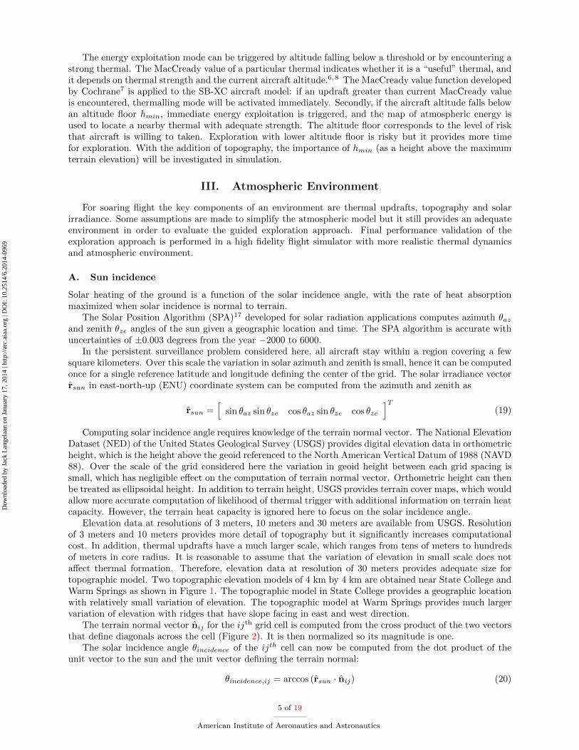
Elevation data at resolutions of 3 meters, 10 meters and 30 meters are available from USGS. Resolutionof 3 meters and 10 meters provides more detail of topography but it significantly increases computationalcost. In addition, thermal updrafts have a much larger scale, which ranges from tens of meters to hundredsof meters in core radius. It is reasonable to assume that the variation of elevation in small scale does notaffect thermal formation. Therefore, elevation data at resolution of 30 meters provides adequate size fortopographic model. Two topographic elevation models of 4 km by 4 km are obtained near State College andWarm Springs as shown in Figure 1. The topographic model in State College provides a geographic locationwith relatively small variation of elevation. The topographic model at Warm Springs provides much largervariation of elevation with ridges that have slope facing in east and west direction.

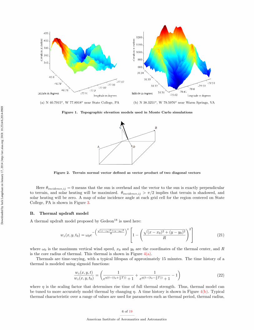
The terrain normal vector nij for the ijth grid cell is computed from the cross product of the two vectorsthat define diagonals across the cell (Figure 2). It is then normalized so its magnitude is one.

The solar incidence angle θincidence of the ijth cell can now be computed from the dot product of theunit vector to the sun and the unit vector defining the terrain normal:

θincidence,ij = arccos (rsun · nij) (20)

5 of 19

American Institute of Aeronautics and Astronautics

Dow

nloa

ded

by J

ack

Lan

gela

an o

n Ja

nuar

y 17

, 201

4 | h

ttp://

arc.

aiaa

.org

| D

OI:

10.

2514

/6.2

014-

0969

(a) N 40.7915o, W 77.8918o near State College, PA (b) N 38.3251o, W 79.5976o near Warm Springs, VA

Figure 1. Topographic elevation models used in Monte Carlo simulations

Figure 2. Terrain normal vector defined as vector product of two diagonal vectors

Here θincidence,ij = 0 means that the sun is overhead and the vector to the sun is exactly perpendicularto terrain, and solar heating will be maximized. θincidence,ij > π/2 implies that terrain is shadowed, andsolar heating will be zero. A map of solar incidence angle at each grid cell for the region centered on StateCollege, PA is shown in Figure 3.

B. Thermal updraft model

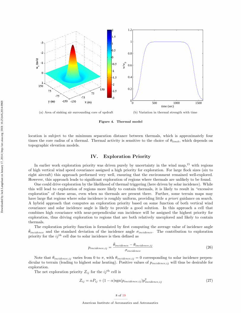
A thermal updraft model proposed by Gedeon18 is used here:

wz(x, y, t0) = ω0e−(√

(x−x0)2+(y−y0)2

R

)21−

(√(x− x0)2 + (y − y0)2

R

)2 (21)

where ω0 is the maximum vertical wind speed, x0 and y0 are the coordinates of the thermal center, and Ris the core radius of thermal. This thermal is shown in Figure 4(a).

Thermals are time-varying, with a typical lifespan of approximately 15 minutes. The time history of athermal is modeled using sigmoid functions:

wz(x, y, t)

wz(x, y, t0)=

(1

eη(t−(t0+12T )) + 1

+1

eη(t−(t0−12T )) + 1

− 1

)(22)

where η is the scaling factor that determines rise time of full thermal strength. Thus, thermal model canbe tuned to more accurately model thermal by changing η. A time history is shown in Figure 4(b). Typicalthermal characteristic over a range of values are used for parameters such as thermal period, thermal radius,

6 of 19

American Institute of Aeronautics and Astronautics

Dow

nloa

ded

by J

ack

Lan

gela

an o

n Ja

nuar

y 17

, 201

4 | h

ttp://

arc.

aiaa

.org

| D

OI:

10.

2514

/6.2

014-

0969

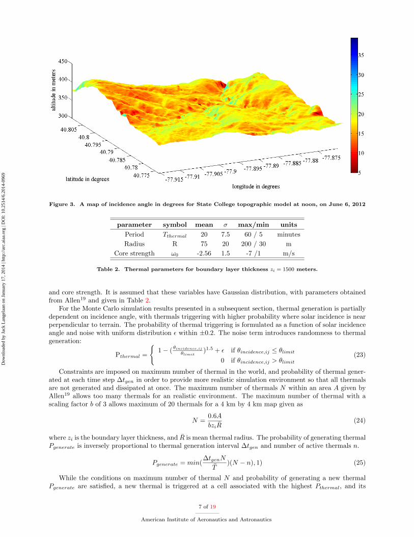
Figure 3. A map of incidence angle in degrees for State College topographic model at noon, on June 6, 2012

parameter symbol mean σ max/min units

Period Tthermal 20 7.5 60 / 5 minutes

Radius R 75 20 200 / 30 m

Core strength ω0 -2.56 1.5 -7 /1 m/s

Table 2. Thermal parameters for boundary layer thickness zi = 1500 meters.

and core strength. It is assumed that these variables have Gaussian distribution, with parameters obtainedfrom Allen19 and given in Table 2.

For the Monte Carlo simulation results presented in a subsequent section, thermal generation is partiallydependent on incidence angle, with thermals triggering with higher probability where solar incidence is nearperpendicular to terrain. The probability of thermal triggering is formulated as a function of solar incidenceangle and noise with uniform distribution ε within ±0.2. The noise term introduces randomness to thermalgeneration:

Pthermal =

{1− (

θincidence,ij

θlimit)1.5 + ε if θincidence,ij ≤ θlimit

0 if θincidence,ij > θlimit(23)

Constraints are imposed on maximum number of thermal in the world, and probability of thermal gener-ated at each time step ∆tgen in order to provide more realistic simulation environment so that all thermalsare not generated and dissipated at once. The maximum number of thermals N within an area A given byAllen19 allows too many thermals for an realistic environment. The maximum number of thermal with ascaling factor b of 3 allows maximum of 20 thermals for a 4 km by 4 km map given as

N =0.6A

bziR(24)

where zi is the boundary layer thickness, and R is mean thermal radius. The probability of generating thermalPgenerate is inversely proportional to thermal generation interval ∆tgen and number of active thermals n.

Pgenerate = min(∆tgenN

T)(N − n), 1) (25)

While the conditions on maximum number of thermal N and probability of generating a new thermalPgenerate are satisfied, a new thermal is triggered at a cell associated with the highest Pthermal, and its

7 of 19

American Institute of Aeronautics and Astronautics

Dow

nloa

ded

by J

ack

Lan

gela

an o

n Ja

nuar

y 17

, 201

4 | h

ttp://

arc.

aiaa

.org

| D

OI:

10.

2514

/6.2

014-

0969

(a) Area of sinking air surrounding core of updraft

0 500 1000 15000

0.2

0.4

0.6

0.8

1

1.2

time (sec)

w/w

0

(b) Variation in thermal strength with time

Figure 4. Thermal model

location is subject to the minimum separation distance between thermals, which is approximately fourtimes the core radius of a thermal. Thermal activity is sensitive to the choice of θlimit, which depends ontopographic elevation models.

IV. Exploration Priority

In earlier work exploration priority was driven purely by uncertainty in the wind map,15 with regionsof high vertical wind speed covariance assigned a high priority for exploration. For large flock sizes (six toeight aircraft) this approach performed very well, ensuring that the environment remained well-explored.However, this approach leads to significant exploration of regions where thermals are unlikely to be found.

One could drive exploration by the likelihood of thermal triggering (here driven by solar incidence). Whilethis will lead to exploration of regions more likely to contain thermals, it is likely to result in “excessiveexploration” of these areas, even when no thermals are present there. Further, some terrain maps mayhave large flat regions where solar incidence is roughly uniform, providing little a priori guidance on search.A hybrid approach that computes an exploration priority based on some function of both vertical windcovariance and solar incidence angle is likely to provide a good solution. In this approach a cell thatcombines high covariance with near-perpendicular sun incidence will be assigned the highest priority forexploration, thus driving exploration to regions that are both relatively unexplored and likely to containthermals.

The exploration priority function is formulated by first computing the average value of incidence angleθincidence and the standard deviation of the incidence angle σincidence. The contribution to explorationpriority for the ijth cell due to solar incidence is then defined as

pincidence,ij =θincidence − θincidence,ij

σincidence(26)

Note that θincidence,ij varies from 0 to π, with θincidence,ij = 0 corresponding to solar incidence perpen-dicular to terrain (leading to highest solar heating). Positive values of pincidence,ij will thus be desirable forexploration.

The net exploration priority Zij for the ijth cell is

Zij = αPij + (1− α)sgn(pincidence,ij)p2incidence,ij (27)

8 of 19

American Institute of Aeronautics and Astronautics

Dow

nloa

ded

by J

ack

Lan

gela

an o

n Ja

nuar

y 17

, 201

4 | h

ttp://

arc.

aiaa

.org

| D

OI:

10.

2514

/6.2

014-

0969

The signum function in the second term of the exploration priority equation indicates that cells withhigher than average solar incidence angles are less likely to contain thermals, and thus are a lower priorityfor exploration.

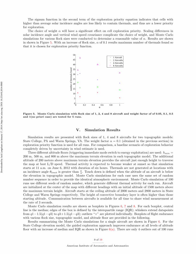
The choice of weight α will have a significant effect on cell exploration priority. Scaling differences insolar incidence angle and vertical wind speed covariance complicate the choice of weight, and Monte Carlosimulations for various flock sizes were conducted to determine a reasonable value of α. Results are shownin shown in Figure 5. With an increase of flock size, α of 0.1 results maximum number of thermals found sothat it is chosen for exploration priority function.

0 0.2 0.4 0.6 0.8 10

5

10

15

20

25

30

35

40

45

50

α

num

ber

of th

erm

als

foun

d

1 Aircraft2 Aircrafts4 Aircrafts8 Aircrafts

Figure 5. Monte Carlo simulation with flock size of 1, 2, 4 and 8 aircraft and weight factor of of 0.05, 0.1, 0.5and 1(no priori case) are tested for 5 runs.

V. Simulation Results

Simulation results are presented with flock sizes of 1, 4 and 8 aircrafts for two topographic models:State College, PA and Warm Springs, VA. The weight factor α = 0.1 (obtained in the previous section) inexploration priority function is used for all runs. For comparison, a baseline scenario of exploration behaviorcompletely driven by uncertainty in wind estimate is used.

Three different altitude floors (triggering immediate mode switch to energy exploitation) are used: hmin =200 m, 500 m, and 800 m above the maximum terrain elevation in each topographic model. The additionalaltitude of 200 meters above maximum terrain elevation provides the aircraft just enough height to traversethe map at best L/D speed. Thermal activity is expected to become weaker at sunset so that simulationstarts at 11 a.m. on June 6, 2012 with duration of six hours. Thermals are not generated at locations withan incidence angle θlimit is greater than π

4 . Touch down is defined when the altitude of an aircraft is belowthe elevation in topographic model. Monte Carlo simulations for each case uses the same set of randomnumber sequence in order to provide the identical atmospheric environment. Monte Carlo simulation of 100runs use different seeds of random number, which generate different thermal activity for each run. Aircraftare initialized at the center of the map with different headings with an initial altitude of 1500 meters abovethe maximum terrain height. Aircraft starts at the ceiling altitude of 2000 meters and 2800 meters in StateCollege and Warm Springs respectively. The height of convective boundary layer is often higher than thosestarting altitude. Communication between aircrafts is available for all time to share wind measurement atthe rate of 3 seconds.

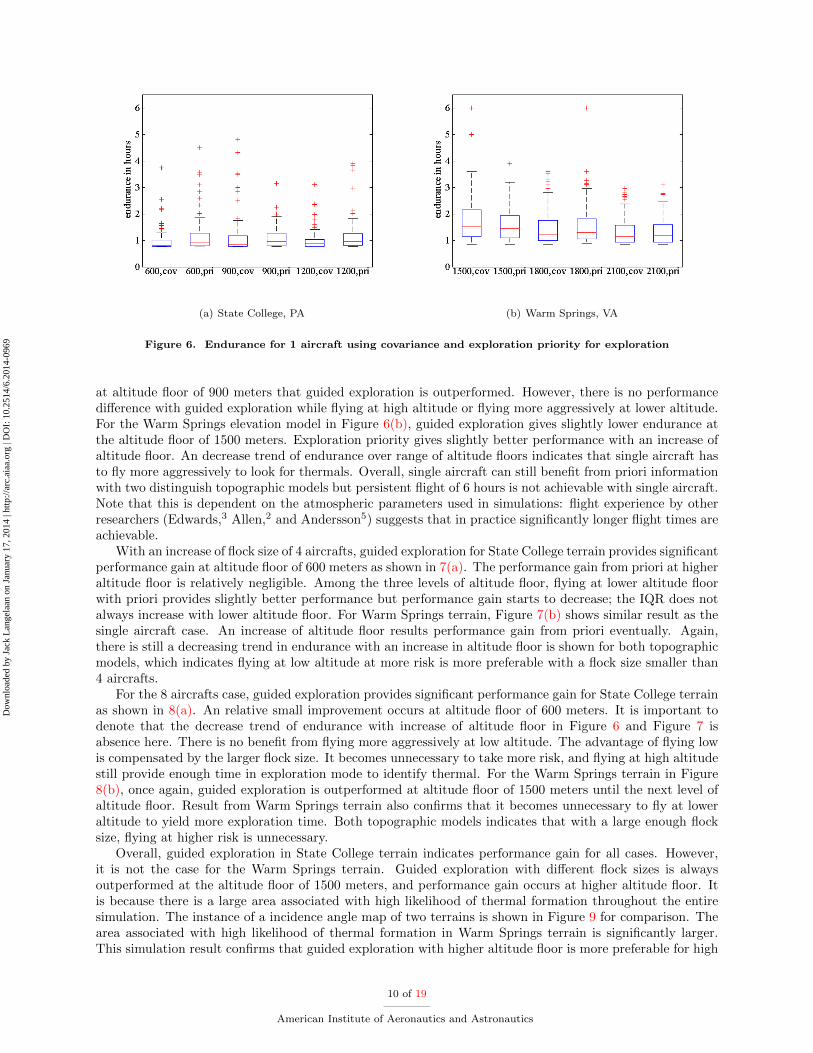
Monte Carlo simulation results are shown as boxplots in Figures 6, 7 and 8. For each boxplot, centralline is the median; edges of the box is defined by the interquartile range (IQR); whiskers extend datapointsfrom q1−1.5(q1−q3) to q3+1.5(q1−q3); outliers “+” are plotted individually. Boxplots of flight endurancewith various flock size, topographic model, and altitude floor are provided in the following.

Results summarizing the Monte Carlo simulations for a single aircraft are shown in Figure 6. For theState College elevation model, the guided exploration approach improves endurance at all levels of altitudefloor with an increase of median and IQR as shown in Figure 6(a). There are only 4 outliers out of 100 runs

9 of 19

American Institute of Aeronautics and Astronautics

Dow

nloa

ded

by J

ack

Lan

gela

an o

n Ja

nuar

y 17

, 201

4 | h

ttp://

arc.

aiaa

.org

| D

OI:

10.

2514

/6.2

014-

0969

(a) State College, PA (b) Warm Springs, VA

Figure 6. Endurance for 1 aircraft using covariance and exploration priority for exploration

at altitude floor of 900 meters that guided exploration is outperformed. However, there is no performancedifference with guided exploration while flying at high altitude or flying more aggressively at lower altitude.For the Warm Springs elevation model in Figure 6(b), guided exploration gives slightly lower endurance atthe altitude floor of 1500 meters. Exploration priority gives slightly better performance with an increase ofaltitude floor. An decrease trend of endurance over range of altitude floors indicates that single aircraft hasto fly more aggressively to look for thermals. Overall, single aircraft can still benefit from priori informationwith two distinguish topographic models but persistent flight of 6 hours is not achievable with single aircraft.Note that this is dependent on the atmospheric parameters used in simulations: flight experience by otherresearchers (Edwards,3 Allen,2 and Andersson5) suggests that in practice significantly longer flight times areachievable.

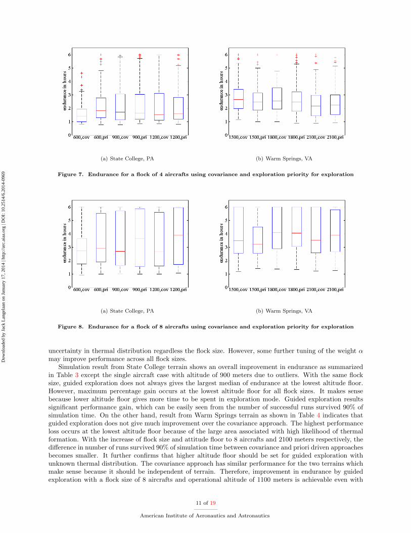
With an increase of flock size of 4 aircrafts, guided exploration for State College terrain provides significantperformance gain at altitude floor of 600 meters as shown in 7(a). The performance gain from priori at higheraltitude floor is relatively negligible. Among the three levels of altitude floor, flying at lower altitude floorwith priori provides slightly better performance but performance gain starts to decrease; the IQR does notalways increase with lower altitude floor. For Warm Springs terrain, Figure 7(b) shows similar result as thesingle aircraft case. An increase of altitude floor results performance gain from priori eventually. Again,there is still a decreasing trend in endurance with an increase in altitude floor is shown for both topographicmodels, which indicates flying at low altitude at more risk is more preferable with a flock size smaller than4 aircrafts.

For the 8 aircrafts case, guided exploration provides significant performance gain for State College terrainas shown in 8(a). An relative small improvement occurs at altitude floor of 600 meters. It is important todenote that the decrease trend of endurance with increase of altitude floor in Figure 6 and Figure 7 isabsence here. There is no benefit from flying more aggressively at low altitude. The advantage of flying lowis compensated by the larger flock size. It becomes unnecessary to take more risk, and flying at high altitudestill provide enough time in exploration mode to identify thermal. For the Warm Springs terrain in Figure8(b), once again, guided exploration is outperformed at altitude floor of 1500 meters until the next level ofaltitude floor. Result from Warm Springs terrain also confirms that it becomes unnecessary to fly at loweraltitude to yield more exploration time. Both topographic models indicates that with a large enough flocksize, flying at higher risk is unnecessary.

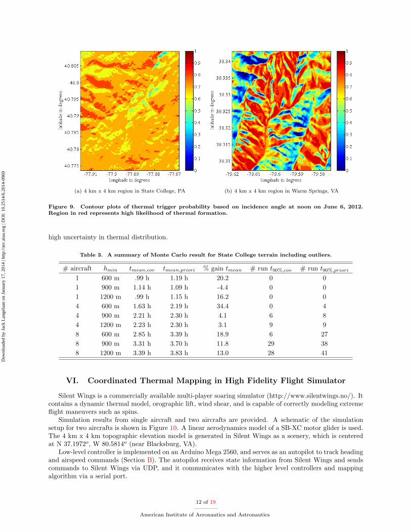
Overall, guided exploration in State College terrain indicates performance gain for all cases. However,it is not the case for the Warm Springs terrain. Guided exploration with different flock sizes is alwaysoutperformed at the altitude floor of 1500 meters, and performance gain occurs at higher altitude floor. Itis because there is a large area associated with high likelihood of thermal formation throughout the entiresimulation. The instance of a incidence angle map of two terrains is shown in Figure 9 for comparison. Thearea associated with high likelihood of thermal formation in Warm Springs terrain is significantly larger.This simulation result confirms that guided exploration with higher altitude floor is more preferable for high

10 of 19

American Institute of Aeronautics and Astronautics

Dow

nloa

ded

by J

ack

Lan

gela

an o

n Ja

nuar

y 17

, 201

4 | h

ttp://

arc.

aiaa

.org

| D

OI:

10.

2514

/6.2

014-

0969

(a) State College, PA (b) Warm Springs, VA

Figure 7. Endurance for a flock of 4 aircrafts using covariance and exploration priority for exploration

(a) State College, PA (b) Warm Springs, VA

Figure 8. Endurance for a flock of 8 aircrafts using covariance and exploration priority for exploration

uncertainty in thermal distribution regardless the flock size. However, some further tuning of the weight αmay improve performance across all flock sizes.

Simulation result from State College terrain shows an overall improvement in endurance as summarizedin Table 3 except the single aircraft case with altitude of 900 meters due to outliers. With the same flocksize, guided exploration does not always gives the largest median of endurance at the lowest altitude floor.However, maximum percentage gain occurs at the lowest altitude floor for all flock sizes. It makes sensebecause lower altitude floor gives more time to be spent in exploration mode. Guided exploration resultssignificant performance gain, which can be easily seen from the number of successful runs survived 90% ofsimulation time. On the other hand, result from Warm Springs terrain as shown in Table 4 indicates thatguided exploration does not give much improvement over the covariance approach. The highest performanceloss occurs at the lowest altitude floor because of the large area associated with high likelihood of thermalformation. With the increase of flock size and attitude floor to 8 aircrafts and 2100 meters respectively, thedifference in number of runs survived 90% of simulation time between covariance and priori driven approachesbecomes smaller. It further confirms that higher altitude floor should be set for guided exploration withunknown thermal distribution. The covariance approach has similar performance for the two terrains whichmake sense because it should be independent of terrain. Therefore, improvement in endurance by guidedexploration with a flock size of 8 aircrafts and operational altitude of 1100 meters is achievable even with

11 of 19

American Institute of Aeronautics and Astronautics

Dow

nloa

ded

by J

ack

Lan

gela

an o

n Ja

nuar

y 17

, 201

4 | h

ttp://

arc.

aiaa

.org

| D

OI:

10.

2514

/6.2

014-

0969

(a) 4 km x 4 km region in State College, PA (b) 4 km x 4 km region in Warm Springs, VA

Figure 9. Contour plots of thermal trigger probability based on incidence angle at noon on June 6, 2012.Region in red represents high likelihood of thermal formation.

high uncertainty in thermal distribution.

Table 3. A summary of Monte Carlo result for State College terrain including outliers.

# aircraft hmin tmean,cov tmean,priori % gain tmean # run t90%,cov # run t90%,priori

1 600 m .99 h 1.19 h 20.2 0 0

1 900 m 1.14 h 1.09 h -4.4 0 0

1 1200 m .99 h 1.15 h 16.2 0 0

4 600 m 1.63 h 2.19 h 34.4 0 4

4 900 m 2.21 h 2.30 h 4.1 6 8

4 1200 m 2.23 h 2.30 h 3.1 9 9

8 600 m 2.85 h 3.39 h 18.9 6 27

8 900 m 3.31 h 3.70 h 11.8 29 38

8 1200 m 3.39 h 3.83 h 13.0 28 41

VI. Coordinated Thermal Mapping in High Fidelity Flight Simulator

Silent Wings is a commercially available multi-player soaring simulator (http://www.silentwings.no/). Itcontains a dynamic thermal model, orographic lift, wind shear, and is capable of correctly modeling extremeflight maneuvers such as spins.

Simulation results from single aircraft and two aircrafts are provided. A schematic of the simulationsetup for two aircrafts is shown in Figure 10. A linear aerodynamics model of a SB-XC motor glider is used.The 4 km x 4 km topographic elevation model is generated in Silent Wings as a scenery, which is centeredat N 37.1972o, W 80.5814o (near Blacksburg, VA).

Low-level controller is implemented on an Arduino Mega 2560, and serves as an autopilot to track headingand airspeed commands (Section B). The autopilot receives state information from Silent Wings and sendscommands to Silent Wings via UDP, and it communicates with the higher level controllers and mappingalgorithm via a serial port.

12 of 19

American Institute of Aeronautics and Astronautics

Dow

nloa

ded

by J

ack

Lan

gela

an o

n Ja

nuar

y 17

, 201

4 | h

ttp://

arc.

aiaa

.org

| D

OI:

10.

2514

/6.2

014-

0969

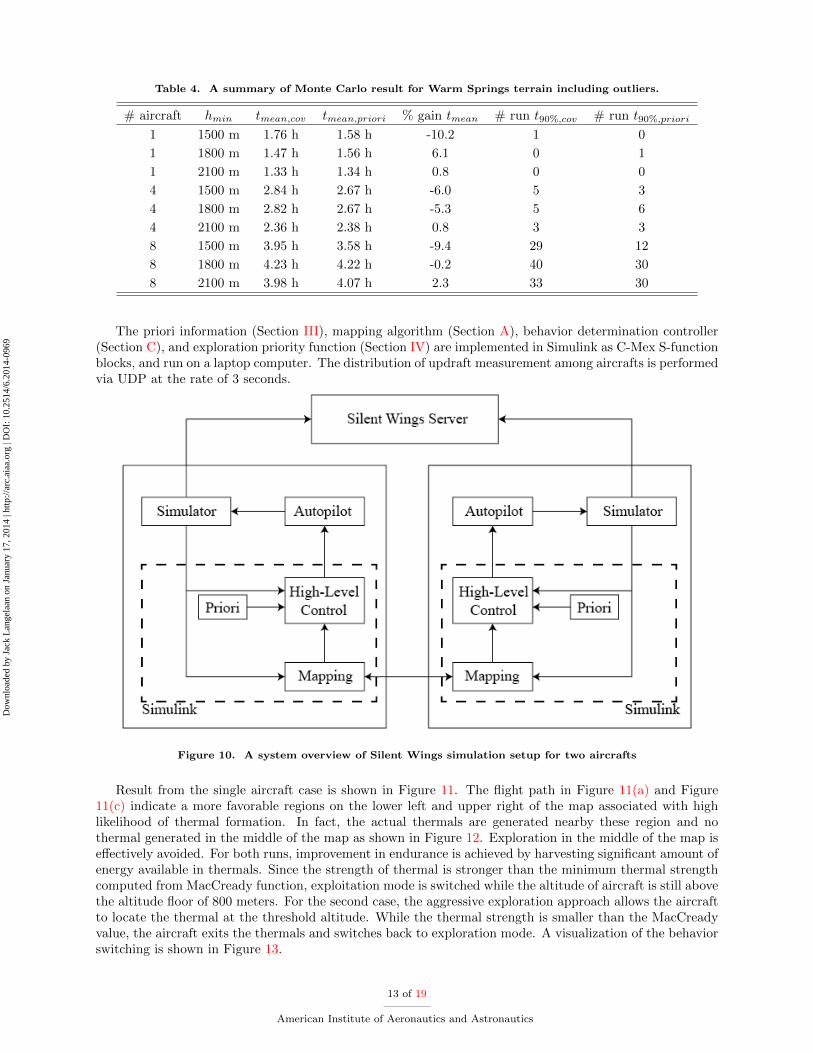
Table 4. A summary of Monte Carlo result for Warm Springs terrain including outliers.

# aircraft hmin tmean,cov tmean,priori % gain tmean # run t90%,cov # run t90%,priori

1 1500 m 1.76 h 1.58 h -10.2 1 0

1 1800 m 1.47 h 1.56 h 6.1 0 1

1 2100 m 1.33 h 1.34 h 0.8 0 0

4 1500 m 2.84 h 2.67 h -6.0 5 3

4 1800 m 2.82 h 2.67 h -5.3 5 6

4 2100 m 2.36 h 2.38 h 0.8 3 3

8 1500 m 3.95 h 3.58 h -9.4 29 12

8 1800 m 4.23 h 4.22 h -0.2 40 30

8 2100 m 3.98 h 4.07 h 2.3 33 30

The priori information (Section III), mapping algorithm (Section A), behavior determination controller(Section C), and exploration priority function (Section IV) are implemented in Simulink as C-Mex S-functionblocks, and run on a laptop computer. The distribution of updraft measurement among aircrafts is performedvia UDP at the rate of 3 seconds.

Figure 10. A system overview of Silent Wings simulation setup for two aircrafts

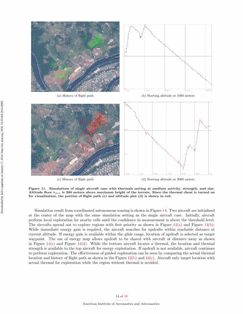
Result from the single aircraft case is shown in Figure 11. The flight path in Figure 11(a) and Figure11(c) indicate a more favorable regions on the lower left and upper right of the map associated with highlikelihood of thermal formation. In fact, the actual thermals are generated nearby these region and nothermal generated in the middle of the map as shown in Figure 12. Exploration in the middle of the map iseffectively avoided. For both runs, improvement in endurance is achieved by harvesting significant amount ofenergy available in thermals. Since the strength of thermal is stronger than the minimum thermal strengthcomputed from MacCready function, exploitation mode is switched while the altitude of aircraft is still abovethe altitude floor of 800 meters. For the second case, the aggressive exploration approach allows the aircraftto locate the thermal at the threshold altitude. While the thermal strength is smaller than the MacCreadyvalue, the aircraft exits the thermals and switches back to exploration mode. A visualization of the behaviorswitching is shown in Figure 13.

13 of 19

American Institute of Aeronautics and Astronautics

Dow

nloa

ded

by J

ack

Lan

gela

an o

n Ja

nuar

y 17

, 201

4 | h

ttp://

arc.

aiaa

.org

| D

OI:

10.

2514

/6.2

014-

0969

(a) History of flight path (b) Starting altitude at 1000 meters

(c) History of flight path (d) Starting altitude at 2000 meters

Figure 11. Simulations of single aircraft case with thermals setting at medium activity, strength, and size.Altitude floor hmin is 200 meters above maximum height of the terrain. Since the thermal cheat is turned onfor visualization, the portion of flight path (c) and altitude plot (d) is shown in red.

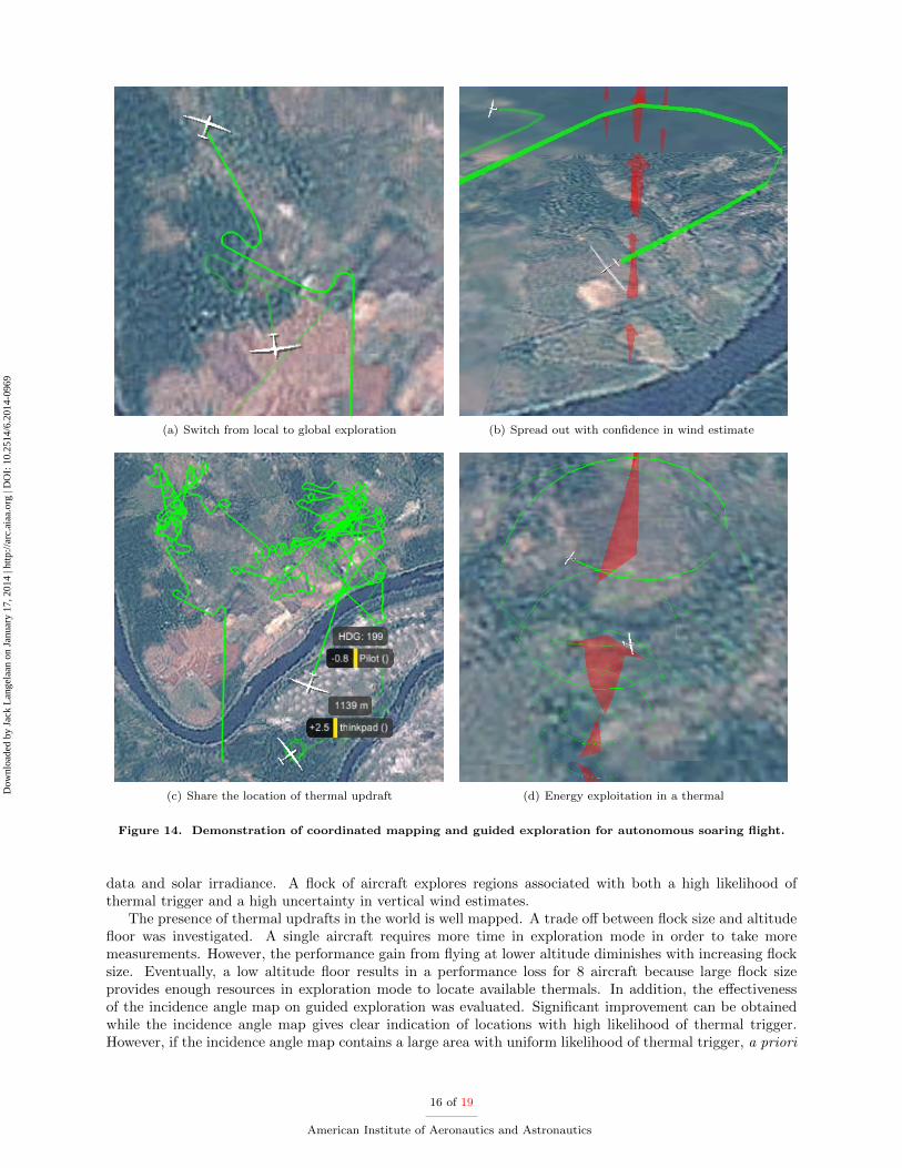
Simulation result from coordinated autonomous soaring is shown in Figure 14. Two aircraft are initializedat the center of the map with the same simulation setting as the single aircraft case. Initially, aircraftperform local exploration for nearby cells until the confidence in measurement is above the threshold level.The aircrafts spread out to explore regions with first priority as shown in Figure 14(a) and Figure 14(b).While immediate energy gain is required, the aircraft searches for updrafts within reachable distance atcurrent altitude. If energy gain is available within the glide range, location of updraft is selected as targetwaypoint. The use of energy map allows updraft to be shared with aircraft at distance away as shownin Figure 14(c) and Figure 14(d). While the bottom aircraft locates a thermal, the location and thermalstrength is available to the top aircraft for energy exploitation. If updraft is not available, aircraft continuesto perform exploration. The effectiveness of guided exploration can be seen by comparing the actual thermallocation and history of flight path as shown in the Figure 12(b) and 14(c). Aircraft only target location withactual thermal for exploration while the region without thermal is avoided.

14 of 19

American Institute of Aeronautics and Astronautics

Dow

nloa

ded

by J

ack

Lan

gela

an o

n Ja

nuar

y 17

, 201

4 | h

ttp://

arc.

aiaa

.org

| D

OI:

10.

2514

/6.2

014-

0969

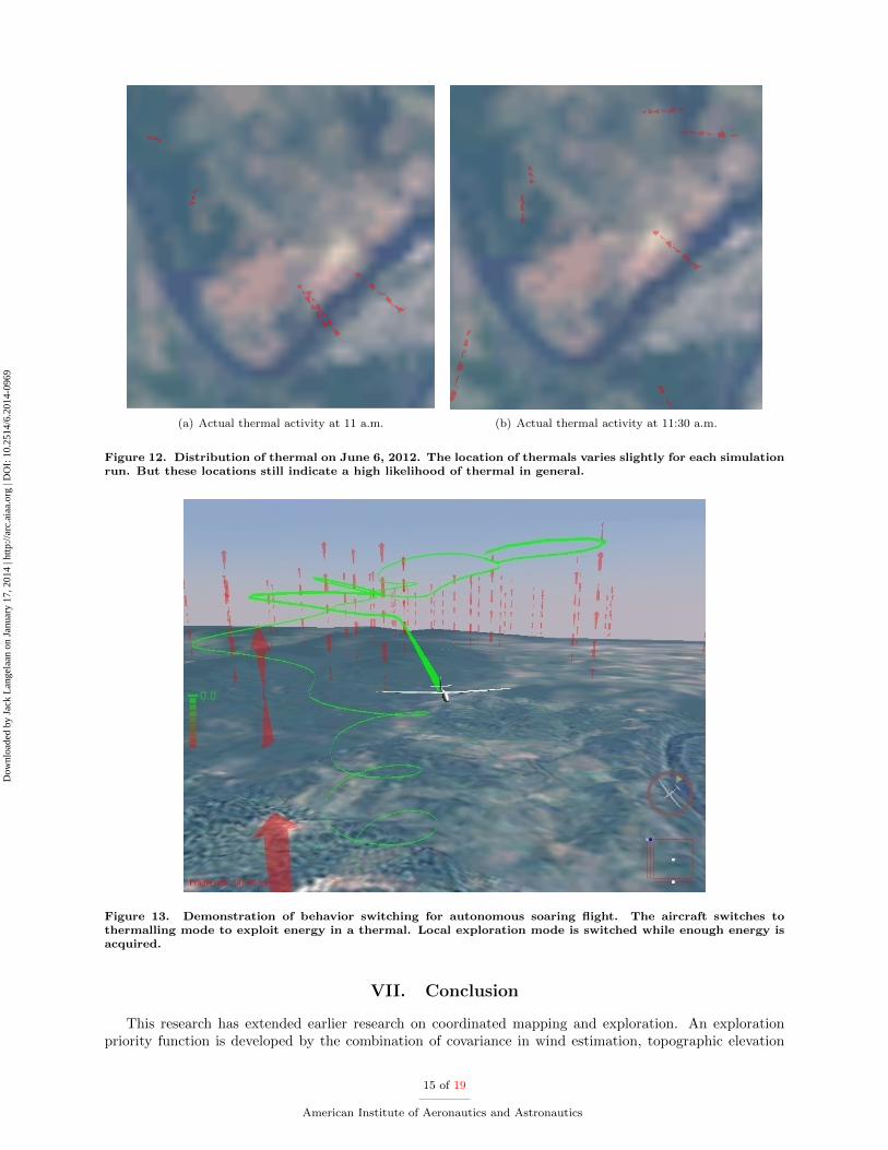
(a) Actual thermal activity at 11 a.m. (b) Actual thermal activity at 11:30 a.m.

Figure 12. Distribution of thermal on June 6, 2012. The location of thermals varies slightly for each simulationrun. But these locations still indicate a high likelihood of thermal in general.

Figure 13. Demonstration of behavior switching for autonomous soaring flight. The aircraft switches tothermalling mode to exploit energy in a thermal. Local exploration mode is switched while enough energy isacquired.

VII. Conclusion

This research has extended earlier research on coordinated mapping and exploration. An explorationpriority function is developed by the combination of covariance in wind estimation, topographic elevation

15 of 19

American Institute of Aeronautics and Astronautics

Dow

nloa

ded

by J

ack

Lan

gela

an o

n Ja

nuar

y 17

, 201

4 | h

ttp://

arc.

aiaa

.org

| D

OI:

10.

2514

/6.2

014-

0969

(a) Switch from local to global exploration (b) Spread out with confidence in wind estimate

(c) Share the location of thermal updraft (d) Energy exploitation in a thermal

Figure 14. Demonstration of coordinated mapping and guided exploration for autonomous soaring flight.

data and solar irradiance. A flock of aircraft explores regions associated with both a high likelihood ofthermal trigger and a high uncertainty in vertical wind estimates.

The presence of thermal updrafts in the world is well mapped. A trade off between flock size and altitudefloor was investigated. A single aircraft requires more time in exploration mode in order to take moremeasurements. However, the performance gain from flying at lower altitude diminishes with increasing flocksize. Eventually, a low altitude floor results in a performance loss for 8 aircraft because large flock sizeprovides enough resources in exploration mode to locate available thermals. In addition, the effectivenessof the incidence angle map on guided exploration was evaluated. Significant improvement can be obtainedwhile the incidence angle map gives clear indication of locations with high likelihood of thermal trigger.However, if the incidence angle map contains a large area with uniform likelihood of thermal trigger, a priori

16 of 19

American Institute of Aeronautics and Astronautics

Dow

nloa

ded

by J

ack

Lan

gela

an o

n Ja

nuar

y 17

, 201

4 | h

ttp://

arc.

aiaa

.org

| D

OI:

10.

2514

/6.2

014-

0969

information is not very useful and the guided exploration approach can be outperformed. Additional tuningof the relative weight between a priori information and the thermal map may improve performance, as wouldincorporating addition information such as terrain albedo. Using a higher altitude floor, guided explorationis able to catch up with covariance approach. Therefore, the confidence in thermal prediction determines thelevel of risk that can be taken. A operational altitude of 1100 meters should be set for an unknown thermaldistribution. Lastly, since all simulation result are generated with gliding flight, additional endurance canbe expected by powering the aircraft to gain altitude before touch down. Long duration flight of six hourswith coordinated autonomous soaring is achievable with small uavs by incorporating priori information.

Autonomous soaring flight in the Silent Wings simulator demonstrates the feasibility of coordinatedsoaring flight in a more realistic atmospheric environment. The exploration priority function avoids a largearea where the likelihood of thermal formation is small. The actual number of thermal is ranging from 4to 7 with medium thermal setting. Both simulation cases are still able to locate thermal with the use ofexploration priority function.

Acknowledgments

This research was funded by the Office of Naval Research under Grant N000141110656. The Arduinoautopilot (The Raptor) was developed by Nathan Depenbusch and Shawn Daugherty from the Air VehicleIntelligence and Autonomy Laboratory (AVIA).

References

1Allen, M. J., “Autonomous Soaring for Improved Endurance of a Small Uninhabited Air Vehicle,” 43rd AIAA AerospaceSciences Meeting and Exhibit , American Institute of Aeronautics and Astronautics, Reno, Nevada, January 2005.

2Allen, M. J. and Lin, V., “Guidance and Control of an Autonomous Soaring Vehicle with Flight Test Results,” AIAAAerospace Sciences Meeting and Exhibit , AIAA Paper 2007-867, American Institute of Aeronautics and Astronautics, Reno,Nevada, January 2007.

3Edwards, D. J., “Implementation Details and Flight Test Results of an Autonomous Soaring Controller,” AIAA Guidance,Navigation and Control Conference, American Institute of Aeronautics and Astronautics, Reston, Virginia, August 2008.

4Anderson, K. and Kaminer, I., “On Stability of a Thermal Centering Controller,” AIAA Guidance, Navigation, andControl Conference, Chicago, Illinois, August 10-13 2009.

5Anderson, K., Kaminer, I., and Jones, K. D., “Autonomous Soaring; Flight Test Results of a Thermal Centering Con-troller,” AIAA Guidance, Navigation and Control Conference, AIAA Paper 2010-8034, American Institute of Aeronautics andAstronautics, Toronto, Canada, August 2010.

6MacCready Jr., P. B., “Optimum Airspeed Selector,” Soaring, January-February 1958, pp. 10–11.7Cochrane, J. H., “MacCready Theory with Uncertain Lift and Limited Altitude,” Technical Soaring, Vol. 23, No. 3, July

1999, pp. 88–96.8Reichmann, H., Cross-Country Soaring, Thomson Publications, Santa Monica, California, 1978.9Arho, R., “Optimal Dolphin Soaring as a Variational Problem,” OSTIV Publication XIII , Organisation Scientifique et

Technique Internationale du Vol a Voile, 1974.10Metzger, D. E. and Hedrick, J. K., “Optimal Flight Paths for Soaring Flight,” Journal of Aircraft , Vol. 12, No. 11, 1975,

pp. 867–871.11Sandauer, J., “Some Problems of the Dolphin-Mode Flight Technique,” OSTIV Publication XV , Organisation Scientifique

et Technique Internationale du Vol a Voile, 1978.12de Jong, J. L., “The Convex Combination Approach: A Geometric Approach to the Optimization of Sailplane Trajecto-

ries,” OSTIV Publication XVI , Organisation Scientifique et Technique Internationale du Vol a Voile, 1981, pp. 182–201.13Pierson, B. L. and Chen, I., “Minimum Altitude Loss Soaring in a Specified Vertical Wind Distribution,” NASA Confer-

ence Publication 2085, Science and Technology of Low Speed and Motorless Flight , edited by P. W. Hanson, NASA, Hampton,Virginia, March 1979, pp. 305–318.

14Sander, G. and Litt, F. X., “On Global Optimal Sailplane Flight Strategy,” NASA Conference Publication 2085, Scienceand Technology of Low Speed and Motorless Flight , edited by P. W. Hanson, NASA, Hampton, Virginia, March 1979, pp.355–376.

15Depenbusch, N. T. and Jack W, L., “Coordinated Mapping and Exploration for Autonomous Soaring,” In-fotech@Aerospace 2011 , AIAA Paper 2011-1436, American Institute of Aeronautics and Astronautics, St. Louis, Missouri,2011.

16Chakrabarty, A. and Langelaan, J. W., “Energy-based Long-range Path Planning for Soaring-capable UAVs,” Journalof Guidance, Control and Dynamics, Vol. 34, No. 4, 2011, pp. 1002–1015.

17Reda, I. and Andreas, A., “Solar Position Algorithm for Solar Radiation Applications,” Tech. rep., National RenewableEnergy Laboratory, Golden, Colorado, 2004.

18Gedeon, J., “Dynamic Analysis of Dolphin Style Thermal Cross Country Flight,” Proceedings of the XIV OSTIVCongress, Organisation Scientifique et Technique Internationale du Vol a Voile, 1974.

17 of 19

American Institute of Aeronautics and Astronautics

Dow

nloa

ded

by J

ack

Lan

gela

an o

n Ja

nuar

y 17

, 201

4 | h

ttp://

arc.

aiaa

.org

| D

OI:

10.

2514

/6.2

014-

0969

19Allen, M. J., “Updraft Model for Development of Autonomous Soaring Uninhabited Air Vehicles,” 44th AIAA Aero-sciences Meeting, AIAA Paper 2006-1510, American Institute of Aeronautics and Astronautics, January 2006.

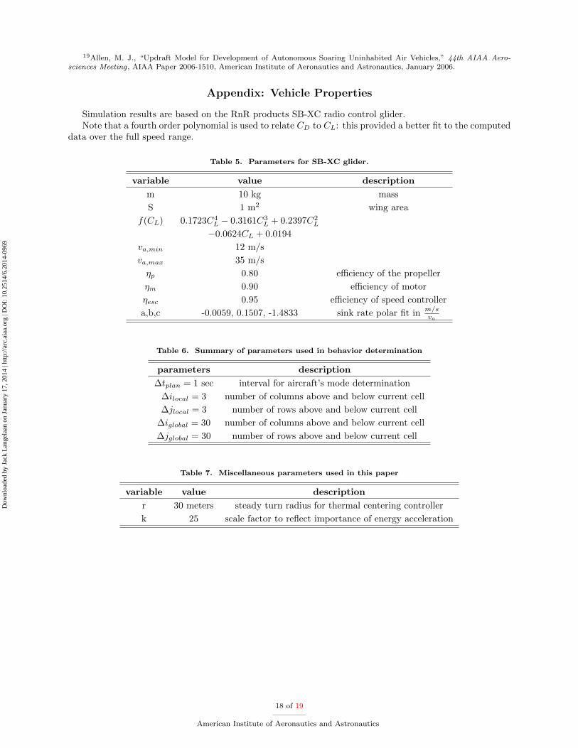
Appendix: Vehicle Properties

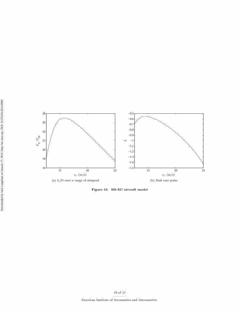
Simulation results are based on the RnR products SB-XC radio control glider.Note that a fourth order polynomial is used to relate CD to CL: this provided a better fit to the computed

data over the full speed range.

Table 5. Parameters for SB-XC glider.

variable value description

m 10 kg mass

S 1 m2 wing area

f(CL) 0.1723C4L − 0.3161C3

L + 0.2397C2L

−0.0624CL + 0.0194

va,min 12 m/s

va,max 35 m/s

ηp 0.80 efficiency of the propeller

ηm 0.90 efficiency of motor

ηesc 0.95 efficiency of speed controller

a,b,c -0.0059, 0.1507, -1.4833 sink rate polar fit in m/sva

Table 6. Summary of parameters used in behavior determination

parameters description

∆tplan = 1 sec interval for aircraft’s mode determination

∆ilocal = 3 number of columns above and below current cell

∆jlocal = 3 number of rows above and below current cell

∆iglobal = 30 number of columns above and below current cell

∆jglobal = 30 number of rows above and below current cell

Table 7. Miscellaneous parameters used in this paper

variable value description

r 30 meters steady turn radius for thermal centering controller

k 25 scale factor to reflect importance of energy acceleration

18 of 19

American Institute of Aeronautics and Astronautics

Dow

nloa

ded

by J

ack

Lan

gela

an o

n Ja

nuar

y 17

, 201

4 | h

ttp://

arc.

aiaa

.org

| D

OI:

10.

2514

/6.2

014-

0969

15 20 2516

18

20

22

24

26

28

va(m/s)

CL /

CD

(a) L/D over a range of airspeed

15 20 25−1.5

−1.4

−1.3

−1.2

−1.1

−1

−0.9

−0.8

−0.7

−0.6

−0.5

va (m/s)

h

(b) Sink rate polar

Figure 15. SB-XC aircraft model

19 of 19

American Institute of Aeronautics and Astronautics

Dow

nloa

ded

by J

ack

Lan

gela

an o

n Ja

nuar

y 17

, 201

4 | h

ttp://

arc.

aiaa

.org

| D

OI:

10.

2514

/6.2

014-

0969