Guide to selecting the appropriate type of light source modelwebcdn.ltioptics.com/photopia-doc-SPIE...
14
Guide to selecting the appropriate type of light source model Mark P. Jongewaard* Lighting Technologies, Inc. Copyright 2002 Society of Photo-Optical Instrumentation Engineers. This paper is published in the proceedings of the SPIE’s 47 th Annual Meeting, Seattle, WA, 2002 and is made available as an electronic preprint with permission of the SPIE. One print or electronic copy may be made for personal use only. Systematic or multiple reproduction, distribution to multiple locations via electronic or other means, duplication of any material in this paper for a fee or for commercial purposes, or modification of the content of the paper are prohibited. ABSTRACT Accurate optical modeling of illumination systems requires, among other things, an accurate characterization of the light sources used in the system. The problem is that there is no single acceptable definition of “accurate” that applies to all circumstances. What is determined to be acceptably accurate must also be tempered with analytical efficiency, meaning that the ideal light source model must contain just enough accuracy to produce acceptable results in the quickest manner possible. Finally, the modeling technique must also be practical to implement given that the technique needs to be applied to the large number of light sources in use today. There are many light source modeling techniques already used in practice and it is worth considering the appropriateness of the various techniques for the applications to which they are being applied. This paper starts with a description of the different aspects of light source models and their modeling techniques. The importance of the different aspects is then summarized for a range of applications. In support of this, data is presented to quantify the sensitivity of the various light source model aspects in the range of applications. The goal of the paper is to present a set of guidelines that can be referenced by designers interested in selecting the most appropriate type of light source model for their range of applications. Keywords: source, lamp, modeling, characterization, selection, techniques, accuracy 1. A DESCRIPTION OF SOURCE MODEL FEATURES Light source models are characterized by their abstractions of the physical nature of the real light sources. The key abstractions are: 1. Geometry 2. Luminous properties 3. Intensity distribution The manner in which these various abstractions are modeled in optical analysis software varies a great deal. Given the range of modeling approaches it is important for the optical designer to understand the nature and limitations of the various approaches so they can ultimately understand the accuracy and value of their optical analysis results. 1.1 Source geometry Light source geometry refers to the representation of the physical size, shape, location, orientation and material of the various parts of the physical light source. The source geometry can also refer to the representation of a purely luminous entity such as an arc in a metal halide source. The source geometry can be used as reference surfaces from which light emanates as well as interacts (reflects, transmits, refracts). Model geometry can be as simple as a point source or as complex as an accurate reproduction of the true mechanical design. The level of detail used can impact the optical analysis results significantly. The most common approaches to modeling source geometry will be classified into 2 main categories, simplified and detailed.
-
Upload
phungduong -
Category
Documents
-
view
213 -
download
1
Transcript of Guide to selecting the appropriate type of light source modelwebcdn.ltioptics.com/photopia-doc-SPIE...

Guide to selecting the appropriate type of light source model
Mark P. Jongewaard*
Lighting Technologies, Inc.
Copyright 2002 Society of Photo-Optical Instrumentation Engineers. This paper is published in the proceedings of the
SPIE’s 47th
Annual Meeting, Seattle, WA, 2002 and is made available as an electronic preprint with permission of the
SPIE. One print or electronic copy may be made for personal use only. Systematic or multiple reproduction, distribution
to multiple locations via electronic or other means, duplication of any material in this paper for a fee or for commercial
purposes, or modification of the content of the paper are prohibited.
ABSTRACT
Accurate optical modeling of illumination systems requires, among other things, an accurate characterization of the light
sources used in the system. The problem is that there is no single acceptable definition of “accurate” that applies to all
circumstances. What is determined to be acceptably accurate must also be tempered with analytical efficiency, meaning
that the ideal light source model must contain just enough accuracy to produce acceptable results in the quickest manner
possible. Finally, the modeling technique must also be practical to implement given that the technique needs to be
applied to the large number of light sources in use today. There are many light source modeling techniques already used
in practice and it is worth considering the appropriateness of the various techniques for the applications to which they are
being applied. This paper starts with a description of the different aspects of light source models and their modeling
techniques. The importance of the different aspects is then summarized for a range of applications. In support of this,
data is presented to quantify the sensitivity of the various light source model aspects in the range of applications. The
goal of the paper is to present a set of guidelines that can be referenced by designers interested in selecting the most
appropriate type of light source model for their range of applications.
Keywords: source, lamp, modeling, characterization, selection, techniques, accuracy
1. A DESCRIPTION OF SOURCE MODEL FEATURES
Light source models are characterized by their abstractions of the physical nature of the real light sources. The key
abstractions are:
1. Geometry
2. Luminous properties
3. Intensity distribution
The manner in which these various abstractions are modeled in optical analysis software varies a great deal. Given the
range of modeling approaches it is important for the optical designer to understand the nature and limitations of the
various approaches so they can ultimately understand the accuracy and value of their optical analysis results.
1.1 Source geometry
Light source geometry refers to the representation of the physical size, shape, location, orientation and material of the
various parts of the physical light source. The source geometry can also refer to the representation of a purely luminous
entity such as an arc in a metal halide source. The source geometry can be used as reference surfaces from which light
emanates as well as interacts (reflects, transmits, refracts). Model geometry can be as simple as a point source or as
complex as an accurate reproduction of the true mechanical design. The level of detail used can impact the optical
analysis results significantly. The most common approaches to modeling source geometry will be classified into 2 main
categories, simplified and detailed.

It is often desirable to make some geometric approximation to the true geometry of a light source or source component.
The approximation can be extreme, as it is in the case of the point source or in the case of using no source geometry at
all. Or the approximation can be more subtle, as in the case of representing a densely coiled filament with a cylinder.
In any case, the net effect of simplified geometry is a loss of detail in regards to the spatial aspect of the model. In order
to retain the spatial detail of the model the geometry can be constructed to be a true representation of the physical source.
Although, even if this approach us used, the model may exclude certain components of the physical source. Whether or
not the excluded components are important to the optical analysis depends on the design.
1.2 Source luminances
Light source luminance refers to the representation of the luminous properties of the source geometry. For example, a
metal halide source model may include a representation of the arc inside of an arc tube, where the arc tube has a white
coating over each of its ends. Both the arc and the white end caps of the arc tube are luminous, but the arc is much
brighter. Assigning luminance values to the arc and white end caps separately allows these differences to be
represented. Further detail can be added by dividing the arc itself into various sections so each can be assigned a unique
luminance.
There are various ways in which source luminances can be assigned and utilized by the raytrace process. In regards to
assigning luminances, they can be assumed to be constant or variable over the extent of particular geometric surfaces. In
regards to utilizing the luminance data, it can drive the general allocation of where rays emanate from a model or it can
additionally drive the amount of light emanated toward a given direction. Some model types allow only constant
luminances across a given surface, but at the same time allow different luminances to be assigned to different surfaces.
More detail in such models means constructing the model from more surfaces. Other model types may allow variable
luminances across particular surfaces, with limited mathematical functions used to describe the variance. Such models
may lend themselves to simpler geometry, but may also have constraints on the geometrical entities that can be used to
construct the model. For example, the luminance may be allowed to vary along the length of a cylinder, but it may not
be allowed to vary over the extent of an arbitrarily shaped polygon.
Another technique used to model source luminances is to use calibrated video images1. This technique involves taking
images of the light source from various points of view in an effort to characterize the changes in luminance across the
source to a high level of detail. See Figure 1 for an example of an image taken of a xenon strobe source.
Figure 1: Video image of xenon strobe source. The source is a glass cylinder with a wire coiled around the outside. The arc is
concentrated toward the left end of the flash tube. The video image was captured by Radiant Imaging, Inc..
In this case the luminance data is not assigned to a particular geometric entity in the model, rather the pixel locations and
the associated luminances imply the physical geometry, but modified according to its optical distortions. For example, if
a view of a filament is distorted when seen through the curved glass of a halogen bulb envelope, then the distorted view
is represented, not the true geometry of the filament.
1.3 Source intensity distribution
Light source intensity distribution refers to the spatial distribution of light emanating from the source. Non-uniform
intensity distributions are typically modeled in 2 ways. The first method is to predict the intensity distribution based on
luminance data of the model. The second method is to use a measured intensity distribution. The general principle of
the first method is to follow the physical law that the total intensity in a given direction is a direct result of the luminous
area exposed to that direction and the absolute luminance of that luminous area. While this method offers a reasonable
approach, the accuracy of the model is a direct function of the model’s ability to accurately depict the true luminous
nature of the source. The general principle of the second method is to bypass the need to accurately describe the true

luminous nature of the source by using the measured intensity distribution directly, regardless of the source properties
that were responsible for creating it.
1.4 Additional considerations
Understanding the features of a source model in regards to geometry, luminance, and intensity distribution will provide
the basis for knowing the abilities and limitations of the source model. But it is equally important to know how the
above listed information is utilized in a particular source model implementation. When all is said and done, the light
source model has 3 main responsibilities to the optical analysis.
1. The model needs to describe the directions toward which rays will be sent.
2. The model needs to describe from what points rays will emanate.
3. The model needs to appropriately interact with light that is redirected back into the light source, either from
other sources or from an optical component such as a reflector.
Given the source intensity distribution via either of the 2 methods described above, an appropriate number of rays will
be sent in all directions surrounding the model. Although implementations may vary, the general process will be as
follows. Assuming that each ray begins with the same number of lumens (source lumens / # of rays to be traced), each
solid angular zone surrounding the source will require a specific number of rays. The lumens per solid angular zone is
given by the luminous intensity in that zone multiplied by the zone solid angle. The rays are in some way distributed
across the zone so that the entire spatial extent is covered. Note that the unit of lumens is assumed for photometric
analyses. Lumens can be replaced by watts for a radiometric analysis. All of the same modeling issues discussed here
apply to both cases.
After a ray direction is defined for a given ray, then an emanation point for that ray must be defined. It might be
assumed that the rays all emanate from some light center point. This assumption completely disregards the spatial extent
from which the light is generated in the physical light source. A more accurate method is to distribute the ray emanation
points across the model geometry in some fashion. This can be done uniformly or non-uniformly. The surface
luminance data is generally used for non-uniform emanation point allocation, where larger and more luminous surfaces
emanate more rays than smaller and less luminous surfaces. Shadowing geometry can also be considered in regards to
ray emanation points. For example the rod, which carries power to the top end of the vertical arc tube in a single ended
HID source, will obscure the view of the arc from a certain range of angles. This essentially limits the luminous area in
view from that range of angles. Different model implementations may or may not account for such an effect when ray
emanation points are selected.
Once a ray direction and emanation point has been defined, then the ray can begin processing in the analysis. If the
model uses the geometry and luminances to determine initial ray directions, then the ray may interact with various
source components before it exits the domain of the source model. In this case, the source geometry would need to
include appropriate optical properties so that the rays could interact with the geometry just as it world with any other
component of the optical system. If the model uses a measured intensity distribution to determine the initial ray
directions, then the ray should not interact with the source model geometry since the effects of such geometry are
already present in the measured intensity distribution. If a ray should happen to be redirected back into the original light
source or into an additional light source present in the design, then the ray has the opportunity to interact with the source
model regardless of how the initial ray was generated. In such a case, the source geometry is treated just like any other
optical component in the design, and thus needs to have specific optical properties appropriate for the physical materials
from which it is comprised. To summarize, whether or not it is necessary to model the geometry and physical properties
of the source components depends on whether or not light ever interacts with it. Light will interact with it both when the
source model depends on such interactions to produce its initial intensity distribution and when light is redirected back
into the source model.
1.5 Summary of source model types
This paper will focus its interest on 3 general types of source models.

Type 1 - Luminance data only (no accompanying model geometry). This type represents the video image based
models. The intensity distribution is goniometric, since it results from the video images from different points of
view. Both the ray emanation points and the intensity distribution of the rays result from direct measurements.
Type 2 - Goniometric intensity distribution with model geometry that includes luminance data. This type of model
distributes ray emanation points across the luminous surfaces of the model geometry in accordance with the relative
luminance values of the various source components. The ray directions are dictated by the measured intensity
distribution. The luminance values can be a result of direct measurement, but distortion effects of luminous surfaces
caused by reflection or refraction are not included.
Type 3 - Self-generated intensity distribution from detailed source geometry and luminance data. This type of
model uses the luminance data for the various surfaces to generate initial rays, which subsequently interact with the
other source components considering the effects of reflection and refraction. This type of source does not use a
measured intensity distribution, but can use measured luminance data. Assuming accurate geometry and luminance
data, this type of model can create accurate luminance data, including distortions caused by reflection or refraction,
as well as an accurate intensity distribution.
2. SOURCE MODEL FEATURE SENSITIVITY FOR VARIOUS APPLICATIONS
The behavior of the complete source model is a result of the interaction of the source geometry, luminous properties and
intensity distribution. This section will provide examples that illustrate the sensitivity of these various features in
various design types. All analysis data presented was generated by the Photopia optical analysis program from Lighting
Technologies, Inc..
2.1 Compact fluorescent lamp (CFL) downlight
A CFL downlight is a design in which a relatively large light source is placed inside a relatively small reflector. The
design requirements must compromise size constraints, visual appearance, beam quality and optical efficiency. Due to
these requirements, a relatively large amount of redirected light inherently interacts with the source. This interaction
between the source and redirected light can have a significant impact on the predicted performance of the design. The
magnitude of the impact depends on the design but is generally related to the relative size of the source with respect to
the size of the reflector. More specifically, it is related to the number of lumens that are redirected back into the source.
Two CFL downlights were analyzed to illustrate these points. The first design uses a 4” diameter cone with a 13W triple
tube CFL. The second design uses a 6” diameter cone with a 32W horizontal CFL. The design geometries are
illustrated in Figure 2.
Figure 2: 4” CFL downlight cone on left, 6” CFL downlight cone on right.

Each design was analyzed with and without the source geometry interacting with the redirected light. In both cases the
initial source rays were identical. The source geometry was removed by assigning perfectly clear transmissive properties
to all of the source components. Keeping the initial source rays identical allows the effects of source geometry
interaction to be isolated. The 2 sets of analyses are therefore intended to compare source models of Type 1 and 2.
Table 1 shows the impact of the source geometry, which includes phosphor coated tubes and a white plastic base, on the
predicted optical efficiency.
Model Description
Efficiency with
Geometry
Efficiency
without
Geometry % Difference
4" Vertical 13W CFL Lamp Downlight 45.7% 55.1% 20.6%
6" Horizontal 32W CFL Lamp Downlight 53.3% 57.0% 6.9%
Table 1: Efficiency prediction summary for CFL downlights.
The 4” diameter design, being more compact, shows a greater impact on the predicted efficiency. But the predicted
efficiency is not the only metric that is affected by the source geometry interaction with the redirected light. The
luminous intensity distribution is also affected, as illustrated in Figure 3. There is no convenient way to characterize the
changes in the intensity distribution with a single value of % difference. Individual angles can be compared but viewing
the overall plot provides the best means of comparison.
Figure 3: The plot on the left shows the 4” CFL downlight luminous intensity distribution. The left half of the plot shows the results
without source geometry and right half shows the results with source geometry. The plot on the right shows the same data for the 6”
CFL downlight.
In regards to the number of lumens that were redirected back into the source, the 4” design had 154% of the source
lumens incident upon the phosphor coated tubes upon redirection. The 6” design had 56% of the source lumens incident
upon the phosphor coated tubes upon redirection. Note that the maximum amount of light that can be redirected back
into the light source surfaces is arbitrarily high. To illustrate this point, consider 1 lumen that leaves the source and is
then reflected from a 90% reflective surface back into the phosphor coated tube. For this single lumen, 90% of it is
redirected back into the tube. Now assume that 80% is reflected from the source tube back to the reflector, and then
back to the source tube again. Added to the initial 0.9 lumens incident upon the tube are 0.9 * 0.8 * 0.9 = 0.648 lumens,
for a total of 1.548 lumens. Thus, due to interreflections, light that was incident upon the source once and then reflected
or transmitted has another chance to be incident upon the source again. The CFL’s in the downlight cones have a large
amount of interreflected light interacting with them. The point to illustrate in this case is that the 4” design had

significantly more light incident upon the source and this was directed related to the magnitude of the changes in
performance seen, especially in regards to the predicted efficiency.
2.2 LED lens design
A lens design for a LED source is a design in which there is generally very little interaction between the redirected light
and the source. The lens design shown in Figure 4 results in only about 2% of the source lumens incident back onto the
LED itself. This increases to 9% when an entire array of LEDs is used instead of just one. This interaction may be
important to some analyses, particularly if controlling stray light is a priority, but in many cases it is likely small enough
to disregard. In such cases, having the detailed source geometry in the model is not as important.
Figure 4: LED with lens array.
What is important in a lens with LEDs in close proximity is both an accurate luminous intensity distribution and an
accurate luminance distribution. The accurate luminance distribution is important because it dictates from where the
rays emanate on the LED. To illustrate the importance of the spatial distribution of the ray emanation points, this design
was analyzed both with a simplified source model and a detailed source model. The simplified model was a Type 2
model that assumed all of the light emanated from the location of the LED chip in the center of the epoxy bulb. The
detailed model was a Type 3 model that used an accurate depiction of the LED geometry and luminous properties of the
chip. The intensity distribution was created in the detailed model by allowing the light to begin at the chip and then
interact with the reflector under the chip and the clear epoxy bulb. This created both an accurate intensity distribution
and an accurate spatial representation of the ray emanation points. Indirectly, the detailed model reproduces the
luminance distribution of the LED as seen from all different viewing angles. Thus, discounting the effects that the
detailed source geometry would have on the light redirected back into the source, the detailed source model would
behave very similar to a source model of Type 1 that is comprised of high resolution video images. The similarities
being that they would both produce the proper luminances at different view angles.
Figure 5 shows the predicted luminous intensity distribution of the LED and lens system. The left half of the plot shows
the results using the simplified source model while the right half shows the results from the detailed source model. Two
planes are shown for each analysis since the lens surface was toroidal providing a different spread in the 0 and 90 degree
planes.
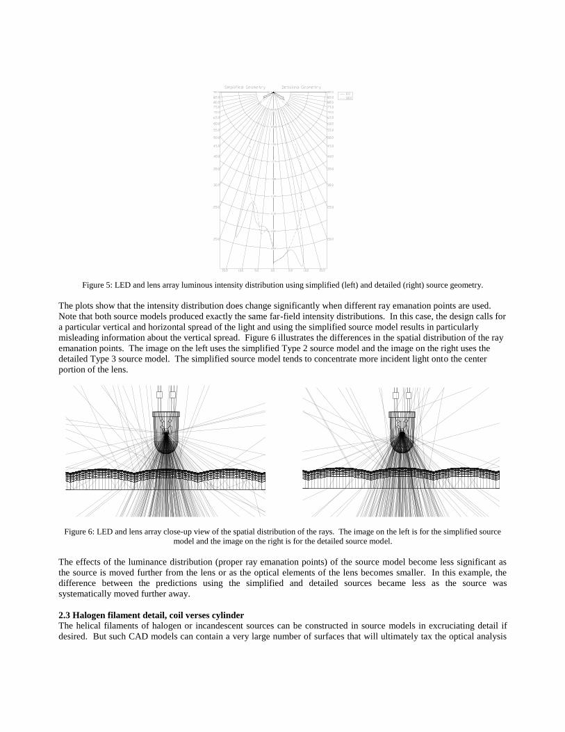
Figure 5: LED and lens array luminous intensity distribution using simplified (left) and detailed (right) source geometry.
The plots show that the intensity distribution does change significantly when different ray emanation points are used.
Note that both source models produced exactly the same far-field intensity distributions. In this case, the design calls for
a particular vertical and horizontal spread of the light and using the simplified source model results in particularly
misleading information about the vertical spread. Figure 6 illustrates the differences in the spatial distribution of the ray
emanation points. The image on the left uses the simplified Type 2 source model and the image on the right uses the
detailed Type 3 source model. The simplified source model tends to concentrate more incident light onto the center
portion of the lens.
Figure 6: LED and lens array close-up view of the spatial distribution of the rays. The image on the left is for the simplified source
model and the image on the right is for the detailed source model.
The effects of the luminance distribution (proper ray emanation points) of the source model become less significant as
the source is moved further from the lens or as the optical elements of the lens becomes smaller. In this example, the
difference between the predictions using the simplified and detailed sources became less as the source was
systematically moved further away.
2.3 Halogen filament detail, coil verses cylinder
The helical filaments of halogen or incandescent sources can be constructed in source models in excruciating detail if
desired. But such CAD models can contain a very large number of surfaces that will ultimately tax the optical analysis

software in some way. Given that many of the helical filaments are quite densely wrapped and approach the shape of a
cylinder, it is worth considering modeling such filaments as cylinders.
If the source model is Type 2, then using the true helix geometry affects only the ray emanation points. If the helical
form is distinct enough, meaning the gaps between the coils are significant, then using the helix for the ray emanation
points may affect some details in the predicted results. For example, in an optic that uses very specular and very smooth
surfaces, distorted views of the helix may be observed in the light pattern. If judging the quality of the beam pattern that
includes such details is important, then using the helical geometry in the source model is required. But if the design will
be evaluated mainly on its candela distribution, then using the exact helical geometry may not be required. Figure 7
shows the cross section of a HX600 halogen source inside of a parabola. The filament is a coiled coil with only 5 turns
over a distance of about 0.46”. Thus, the helix leaves relatively large open spaces between the coils.
Figure 7: HX600 source inside of a parabola.
Figures 8 and 9 show the predicted performance of this design using both a helix based source model and a hollow
cylinder based source model. Figure 8 shows a shaded plot of the illuminance pattern on a 2’ x 2’ plane, 4’ away.
Figure 9 shows the axially averaged luminous intensity plot for each source model.
Figure 8: Shaded illuminance pattern using helical model (left) and cylindrical model (right) for the source filament.

HX600 in Parabola Candela Distribution
0
50000
100000
150000
200000
250000
300000
350000
400000
0 5 10 15 20 25 30
Vertical Angle (degrees)
Can
dela
s
Helix
Cylinder
Figure 9: Luminous intensity plot for helical and cylindrical based filament models.
The illuminance plot shows the effects of the helical filament as a spiraled pattern. This effect is of course missed when
the cylindrical filament is used. If judging solutions to eliminate the spiral effect is part of the design problem, then the
helical filament model is certainly needed. In regards to the luminous intensity distribution, the value in the center of the
distribution decreased by only 3.2% when the cylindrical filament was used. Note however, that the center beam
intensity is very sensitive to the exact length of the cylinder. In this case, a cylinder was used that fully encompassed the
helix. Nonetheless, if judging the intensity distribution is the only requirement, then the helical filament is not needed.
In regards to the model complexity, the helical filament based model required a total of 3067 polygonal surfaces to
describe. Recall that this was for a helix with only 5 turns. This would extrapolate to a very large number if a tightly
wound filament with 40 turns were used instead. The model using the cylindrical filament required only 683 polygonal
surfaces. In a raytracer where the speed is linearly related to the number of surfaces in the model, this will increase the
calculation time accordingly. In a raytracer that is optimized so that the surface count has little impact on the calculation
speed, then this may not be such an important issue.
If the source model is Type 3, then using the true helix geometry affects both the ray emanation points as well as the
generation of the source intensity distribution. The filaments have a higher luminance on the inside compared to the
outside and the ends of the helix are typically less luminous than the central coils. All of these details affect the resulting
intensity distribution and if the true helix geometry is not used then novel luminance distributions must be given to the
surfaces of the cylinder that approximates the filament. The novel luminance distributions must replicate the observed
luminous behavior of the filament as the coil shadows itself by various amounts at various view angles thus exposing
different amounts of the higher inside luminances and lower outside luminances.
2.4 Filament/Arc distortions due to bulb wall refraction
When filaments or arcs are viewed through the curved portions of their clear bulbs then the view of their associated
luminances becomes distorted. This effects both the luminous intensity distribution and the spatial luminances of the
source. Type 1 and Type 3 source models characterize both of these effects. Type 2 source models include the effects
on the intensity distribution but do not characterize the distorted spatial luminances. However, whether or not it is
important that the source model include both effects depends on the application. If the reflector or other optical
component receives light from a “capture angle” that does not include the areas of the bulb that distort the views, then
the source model does not need to include the distorted spatial luminances. Figure 10 shows 2 reflectors and their
associated capture angles.

Figure 10: Capture angle of a 38-degree MR-16 (left) and a 30-degree ceramic metal halide spot reflector.
The MR-16 reflector does receive some light that will be refracted by the bulb wall, especially near the base of the
source. So the analysis of the MR-16 might benefit from a Type 1 or Type 3 source model. The ceramic metal halide
based reflector receives its light through a clear section of the bulb, thus making any of the 3 source model types
acceptable.
3. LIGHT SOURCE MODEL CONSTRUCTION CONSIDERATIONS
3.1 Type 1 source models
Type 1 source modeling methods are well established so they will not be repeated here1. However, it is important to
mention some issues that affect their applicability. Some of the effects that Type 1 models are so well suited to capture
are also effects that are inconsistent from one source sample to the next. The distortions created by the curved bulb
walls or pinched tips of the bulbs are good examples. Personally viewing 3 samples of the same halogen source type
will illustrate this point. Another issue is the deposits on the arc tube of a metal halide source. The deposits are a result
of the chemicals required to make the metal halide source work. But the deposits can effect the transmission through the
arc tube significantly. Furthermore, they change from 1 source sample to the next, they do not fully evaporate when the
source is operating, and they change position depending upon the orientation of the source. Since they affect the source
luminances seen from various points of view they also effect the source intensity distribution, which is an issue for Type
2 source models as well. If a Type 1 model is used for a source type that is affected by these issues, then it is best to
have more than a single source sample modeled so that either an average model can be constructed or so that more than
1 specific source sample can be processed in the optical analysis to see how the results change. Figure 11 illustrates how
the luminous intensity distribution can change from source to source. The plots are for 3 samples of a vertical filament
50W halogen source. The plots show all of the measured horizontal planes of data for each source sample. All plots are
shown on the same scale.

Figure 11: Luminous intensity plots for 3 samples of a 50W vertical filament halogen source.
3.2 Type 2 source models Type 2 source models are intended to be a compromise between ease of construction and possessing an adequate level of
accuracy. The models use far-field photometry for their intensity distribution, facilities for which are widely available.
The luminance data is generally straightforward to collect by either direct measurement or by means of projection of an
image of very small sources. Only relative luminance data is required. The physical geometry must be directly
measured or obtained from the source manufacturer. The geometry however, can be simplified to include only that
which is considered to be optically important. For ray emanation, this includes only the luminous parts of the source.
For secondary ray interactions, the bulb and major support structure can be included as well. The geometrical accuracy
affects only the ray emanation points. Thus, precise accuracy is not needed in the same way a Type 3 model requires,
where it also effects the intensity distribution.
3.3 Type 3 source models Type 3 source models can be straightforward to create for certain source types such as most fluorescents, some halogens
and some HID sources. But for other source types, measuring the important parameters required to construct the model
is impractical and thus forces approximations. This leads to either an inaccurate model or one that requires a lot of trial
and error to get working properly. The same issues listed above in regards to the Type 1 models are what can make
Type 3 source modeling difficult. In order for the Type 3 model to be checked for its accuracy, it should be capable of
reproducing a measured intensity distribution. If the measured intensity distribution is effected by such inconsistent
parameters such as the exact curvature of a bulb wall or the exact deposits on the arc tube of a metal halide source, then
such intensity distributions will be difficult to match. But even if the model details are determined so that they do match
the measured intensity distributions for such inconsistent sources, then only a single source sample is represented. With
Type 1 or Type 2 source models a different source sample can quickly be modeled with a new measurement set. For the
Type 1 source model a new set of video images is required. For the Type 2 source model a new intensity distribution is
required. With a Type 3 model, new geometry or new luminance parameters need to be determined via more trial and
error or relatively tedious measurements.
The construction of Type 3 bulb style LED models is especially difficult because some of the key aspects of the source
are not directly measurable. In particular, the luminous properties of the LED chip and the shape of the embedded
reflector are difficult or impossible to measure. The outer bulb shape is the only parameter that is practical to measure.
The only way to determine the parameters that cannot be directly measured is by trial and error. A guess at the
parameters is made and the model performance is tested against the measured luminous intensity distribution. Values
for the parameters are continually refined until satisfactory accuracy is obtained.
4. SELECTION GUIDE FOR THE APPROPRIATE TYPE OF SOURCE MODEL
Given the range of source modeling methods available and the potential impact different methods can have on the
predicted results, it is important that the optical designer fully understand what methods are available in their optical
analysis software. Furthermore, the implementation details of the particular modeling methods should be understood.

This information will help the designer select the best type of source model for their particular application if they have a
choice and understand the potential consequences to their predicted results when a non-ideal source model must be used.
Although there are a lot of small details that may effect the final decision about the best type of source model for a given
application, it is the author’s opinion that the most critical issues are summarized in the following 3 questions:
1. Does the real source have refractive or reflective effects that distort the luminous views of the arc or filament?
2. If luminance distortions are present, then do they affect the light directed toward the primary optical control
components such as a reflector or a lens?
3. Is the source geometry required? If there are significant interactions between the source and redirected light or
light from another source, then the answer is ‘yes.’
Using the answers to these 3 questions, the most appropriate type of source model can determined. Or as the chart that is
presented in Figure 12 indicates, the most inappropriate type of source model can be determined. The reason for this last
statement is because in most instances more than one type of source model is sufficient for the task. In these cases the
utility of the chart is to indicate where certain source model types should not be used.

Q1:
Luminance
distortions?
Q2:
Distortions
affect
optics?
Q3: Lamp geometry
required?
Q3: Lamp geometry
required?
Q3: Lamp geometry
required?
Yes
Yes
YesYes
Yes
No
No
No
No No
Type 1, 2 or 3 Type 2 or 3
Type 2 or 3 Type 1 or 3 Type 3
LIGHT SOURCE MODEL SELECTION GUIDE
Figure 12: Light source model selection guide.

From a theoretical standpoint, the Type 3 source model appears to meet the needs of most situations. In fact, the Type 3
source model shows up as being appropriate for every situation in the chart. But the practical limitations of creating
such source models limit its utility. Thus, when a Type 3 source model is not absolutely needed, Type 1 or Type 2
source models become a better choice. Note that there is only 1 place on the chart where the Type 3 source model is the
only type recommended.
There is one other topic to consider when selecting between different types of source models that are all appropriate for a
given application. This is the issue of the required accuracy. Of course the highest level of accuracy is always desired,
but is it always required? To answer this question more meaningfully, consider the following questions about the given
application:
1. What is the application of the predicted data? If the data is for internal evaluations of the product performance
early in the design process, then a more approximate source model can be tolerated. As the design becomes
more refined then more detail is required of the source model. If the predicted photometric data is to be sent to
customers as a representation of the product performance they should expect, then the most care should be
taken to use an accurate source model.
2. What is the accuracy of the manufactured product? If the manufactured parts that will comprise the final optic
will not be held to a high level of precision, then the accuracy of the source model becomes less important.
Formed or rolled sheet metal optics are typical of surfaces that may significantly stray from their designed
shapes. Lamp position is another parameter that can sometimes vary from the design. This is particularly true
when the sources are extended on long support arms or when relatively long sources are mounted in imprecise
screw bases such as medium and mogul bases.
3. What types of materials are used on the optical control surfaces? The most optical control is provided by the
most specular reflector surfaces and by the most highly polished lens or refractor surfaces. If the reflector is to
be constructed from non-specular materials or if the lens is to be made from non-clear materials, then precise
performance of the source model becomes less important. When light scattering materials are used the source
model can contain less accurate spatial luminance data, for example, and still produce adequate results.
REFERENCES
1. R. Rykowski, B. Wooley, “Source Modeling for Illumination Design,” Proceedings of SPIE, Vol. 3130, 1997.
*[email protected]; phone 1 (720) 891-0030; fax 1 (720) 891-0031; www.lighting-technologies.com;
Lighting Technologies, Inc., 1630 Welton Street, Suite 400, Denver, Colorado, USA 80202