Guidance for Flood Risk Analysis and Mapping - Home | … · 2016-08-24 · Guidance for Flood Risk...

Guidance for Flood Risk Analysis and Mapping

Coastal Water Levels

May 2016

Water Levels May 2016 Guidance Document 67 Page i

Requirements for the Federal Emergency Management Agency (FEMA) Risk Mapping, Assessment, and Planning (Risk MAP) Program are specified separately by statute, regulation, or FEMA policy (primarily the Standards for Flood Risk Analysis and Mapping). This document provides guidance to support the requirements and recommends approaches for effective and efficient implementation. Alternate approaches that comply with all requirements are acceptable.

For more information, please visit the FEMA Guidelines and Standards for Flood Risk Analysis and Mapping webpage (www.fema.gov/guidelines-and-standards-flood-risk-analysis-and-mapping). Copies of the Standards for Flood Risk Analysis and Mapping policy, related guidance, technical references, and other information about the guidelines and standards development process are all available here. You can also search directly by document title at www.fema.gov/library.

http://www.fema.gov/guidelines-and-standards-flood-risk-analysis-and-mapping

http://www.fema.gov/guidelines-and-standards-flood-risk-analysis-and-mapping

http://www.fema.gov/library

Water Levels May 2016 Guidance Document 67 Page ii

Document History

Affected Section or Subsection Date Description

First Publication May 2016

Initial version of new transformed guidance. The content was derived from the Guidelines and Specifications for Flood Hazard Mapping Partners, Procedure Memoranda, and/or Operating Guidance documents. It has been reorganized and is being published separately from the standards.

Water Levels May 2016 Guidance Document 67 Page iii

Table of Contents 1.0 Topic Overview .................................................................................................................. 1

2.0 Astronomic Tide ................................................................................................................. 1

2.1 Tides and Tidal Datums .................................................................................................. 1

3.0 Storm Surge Modeling ....................................................................................................... 4

3.1 General Considerations .................................................................................................. 5

3.2 Mesh Considerations ...................................................................................................... 6

3.3 Boundary Forcing ........................................................................................................... 7

3.4 Astronomical Tidal Effects in Storm Surge Analysis ....................................................... 8

3.5 Wind Drag and Bottom Drag ........................................................................................ 13

3.6 Land Cover Data .......................................................................................................... 14

3.7 Wave Setup .................................................................................................................. 14

3.8 Storm Climatology ........................................................................................................ 14

3.9 Measured Water Level Data ......................................................................................... 14

3.10 Ice Cover ...................................................................................................................... 16

3.11 Model Validation ........................................................................................................... 17

4.0 Water Levels in Sheltered Waters .................................................................................... 20

4.1 Variability of Tide and Storm Surge in Sheltered Waters ............................................. 20

4.2 Seiche ........................................................................................................................... 22

4.3 Estimating Sheltered Water Levels Using Existing Flood Insurance Study Data ......... 22

5.0 Nonstationary Processes ................................................................................................. 24

5.1 Relative Sea Level – Sea Level Rise ........................................................................... 25

5.2 Relative Sea Level – Land Subsidence and Rebound ................................................. 25

5.3 Astronomic Tide Variation ............................................................................................ 25

6.0 References ....................................................................................................................... 26

List of Figures Figure 1. Tidal datum information for Los Angeles, CA. ............................................................... 2

Figure 2. Predicted, Observed, and Residual Tides at Panama City, Florida ............................. 15

Water Levels May 2016 Guidance Document 67 Page 1

1.0 Topic Overview This guidance document supports the standards related to the determination of coastal stillwater levels (SWLs). The SWL is a coastal water surface resulting from astronomical tides, storm surge, and, depending on the location, other effects such as El Niño effects or seiching. The SWL does not include wave heights and runup. The stillwater elevation (SWEL) is the statistical elevation of the SWL relative to a specified datum. The statistical methods needed to determine the 1%-annual-chance SWEL are discussed in FEMA’s Coastal Flood Frequency Analysis Guidance document. The mean water level (MWL) includes all components contributing to the SWL plus static wave setup. The dynamic water level (DWL) is the combination of SWL plus static and dynamic wave setup; this generally applies only to studies on the Pacific coast. Coastal Base Flood Elevations (BFEs) are a combination of waves or runup on top of the SWELs.

Depending on the coastal location, the SWL historically included wave components. On the Atlantic and Gulf coasts, the SWL included astronomic tides as well as storm surge and wave setup that are developed during large tropical and extra-tropic storm events. On the Great Lakes, the tidal component is so minimal to be excluded from the SWL and only storm surge and wave setup were included in the calculations. On the Pacific coast, the surge components driven by barometric pressure changes and El Niño effects can be captured in tide station records. In the Pacific studies dynamic wave setup was added. Inclusion of wave setup would include the word ‘Total’ in the definition of SWL or SWEL.

This guidance document discusses astronomic tides and the process of extracting SWL data from those records in Section 2. For areas where storm surge processes dominate, guidance on how to determine the SWL from storm surge effects is provided in the Section 3. Section 3 includes a discussion on the inclusion of tides for surge-dominated coastal areas. Sheltered waters and non-stationary effects are discussed in Sections 4 and 5, respectively.

2.0 Astronomic Tide The astronomic tide is the regular rise and fall of the ocean surface in response to the gravitational influence of the moon, the sun, and the Earth. Because the astronomic processes are entirely regular, the tides, too, behave in an entirely regular, though complex, manner.

The statistical analysis of tide gage data is discussed in the Coastal Flood Frequency Analysis Guidance document.

2.1 Tides and Tidal Datums The tides along the Atlantic are semi-daily or semidiurnal, meaning that there are two highs and two lows each day, while in the Gulf of Mexico the tides are mix of diurnal, meaning that there is only one high and low each day, and semidiurnal. The tides along the Pacific Coast are mixed and semi-diurnal; conventionally, mixed tides are semi-diurnal tides for which the magnitudes of successive highs or successive lows have large variation. The average of all the highs is denoted as mean high water (MHW) while the average of all the lows is mean low water (MLW). Averages are taken over the entire tidal datum epoch, which is a particular 19-year period explicitly specified for the definition of the datums; a full astronomic tidal cycle covers a period of 18.6 years. The average of all hourly tides over the epoch is the mean sea level (MSL).


The daily highs are generally unequal, as are the lows, and are identified as Higher High, Lower High, and so forth. At a given coastal location, each of these has a mean value identified as mean higher high water (MHHW), mean lower high water (MLHW), mean higher low water (MHLW), and mean lower low water (MLLW). In addition to these, there is the mean tide level (MTL) which is the average of MHW and MLW, and which is also called the half-tide level.

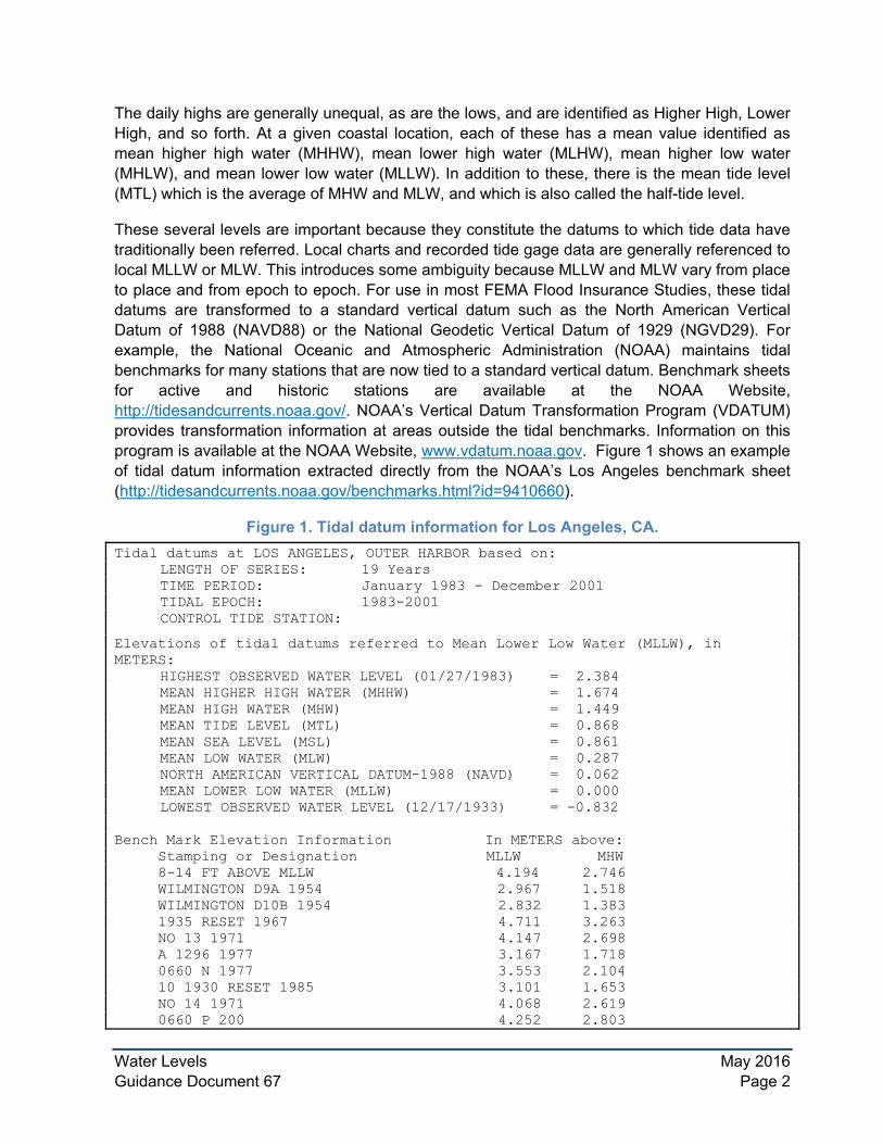
These several levels are important because they constitute the datums to which tide data have traditionally been referred. Local charts and recorded tide gage data are generally referenced to local MLLW or MLW. This introduces some ambiguity because MLLW and MLW vary from place to place and from epoch to epoch. For use in most FEMA Flood Insurance Studies, these tidal datums are transformed to a standard vertical datum such as the North American Vertical Datum of 1988 (NAVD88) or the National Geodetic Vertical Datum of 1929 (NGVD29). For example, the National Oceanic and Atmospheric Administration (NOAA) maintains tidal benchmarks for many stations that are now tied to a standard vertical datum. Benchmark sheets for active and historic stations are available at the NOAA Website, http://tidesandcurrents.noaa.gov/. NOAA’s Vertical Datum Transformation Program (VDATUM) provides transformation information at areas outside the tidal benchmarks. Information on this program is available at the NOAA Website, www.vdatum.noaa.gov. Figure 1 shows an example of tidal datum information extracted directly from the NOAA’s Los Angeles benchmark sheet (http://tidesandcurrents.noaa.gov/benchmarks.html?id=9410660).

Figure 1. Tidal datum information for Los Angeles, CA. Tidal datums at LOS ANGELES, OUTER HARBOR based on:

LENGTH OF SERIES: 19 Years TIME PERIOD: January 1983 - December 2001 TIDAL EPOCH: 1983-2001 CONTROL TIDE STATION:

Elevations of tidal datums referred to Mean Lower Low Water (MLLW), in METERS:

HIGHEST OBSERVED WATER LEVEL (01/27/1983) = 2.384 MEAN HIGHER HIGH WATER (MHHW) = 1.674 MEAN HIGH WATER (MHW) = 1.449 MEAN TIDE LEVEL (MTL) = 0.868 MEAN SEA LEVEL (MSL) = 0.861 MEAN LOW WATER (MLW) = 0.287 NORTH AMERICAN VERTICAL DATUM-1988 (NAVD) = 0.062 MEAN LOWER LOW WATER (MLLW) = 0.000 LOWEST OBSERVED WATER LEVEL (12/17/1933) = -0.832

Bench Mark Elevation Information In METERS above: Stamping or Designation MLLW MHW 8-14 FT ABOVE MLLW 4.194 2.746 WILMINGTON D9A 1954 2.967 1.518 WILMINGTON D10B 1954 2.832 1.383 1935 RESET 1967 4.711 3.263 NO 13 1971 4.147 2.698 A 1296 1977 3.167 1.718 0660 N 1977 3.553 2.104 10 1930 RESET 1985 3.101 1.653 NO 14 1971 4.068 2.619 0660 P 200 4.252 2.803

http://tidesandcurrents.noaa.gov/

http://www.vdatum.noaa.gov/

http://tidesandcurrents.noaa.gov/benchmarks.html?id=9410660


In this example, NAVD88 is shown to be at 0.062 meters above MLLW for the specified 1983-2001 epoch. Not all benchmark sheets include NAVD88 (or NGVD29) as this example does, but most include surveyor’s benchmark information through which the tidal datums can usually be tied to a standard vertical datum; these benchmark sheets include full descriptions of the benchmarks and exact locations.

Outside of the continental U.S., other orthometric datums are used. These include the American Samoa Vertical Datum of 2002 (ASVD02), Guam Vertical Datum of 2004 (GUVD04), Northern Marianas Vertical Datum of 2003 (NMVD03) and Puerto Rico Vertical Datum of 2002 (PRVD02). Additionally, Virgin Islands Vertical Datum of 2009 (VIVD09) will soon be published and a new Hawaii vertical datum is in the planning stage. Because these locations do not tie-in to the NAVD88 datum, FEMA studies in these areas often use the Local Mean Sea Level datum.

The Great Lakes are subject to the same astronomical forces that produce the tides observed along the ocean shoreline. The Canadian Hydrologic/Hydrographic Service reports a tidal response of less than 2 inches in the Great Lakes, the strongest being on Lakes Superior and Erie. These fluctuations are so small that their presence is masked by the water body’s normal fluctuations due to atmospheric forcing. For all practical purposes and in FEMA Flood Insurance Studies, the Great Lakes can be treated as if no tidal signal exists.

In summary, the Mapping Partner is responsible for relating data to a standard vertical datum and should utilize the most appropriate resources available to them to do so.

2.1.1 Tide Observations The tide is recorded at a large number of gages throughout the Atlantic, Gulf of Mexico, and Pacific coastlines, with records dating back over 100 years in many cases. Much of this data is available at NOAA’s website for the National Water Level Observation Network, modeling, as either six-minute or hourly time series over the particular site’s entire period of record. Additional data may be available from other sources including The United States Geological Survey (USGS), the United States Army Corps of Engineers (USACE), or others.

Tidal observations at the gage are usually suitably filtered to suppress high frequency wave components, but do include the long period components associated not only with astronomic tide, but also with sea level variations caused by atmospheric pressure fluctuations, wind setup (storm surge), riverine rainfall runoff into a relatively confined region, low frequency tsunami elevation, seiche, and wave setup to the degree that it occurs at the gage site. In general, gages are often located in protected areas not subject to much setup, or in open areas outside the surf zone, and so seaward of the largest setup values.

The fact that the tide gage record includes all of these non-astronomic low frequency components makes it possible to extract SWEL statistics from gage data, subject to the setup limitation noted.

2.1.2 Tide Predictions The astronomic component of the observed tide gage record is considered to be well-known in principle, consisting of the summation of 37 tidal constituents that are simply sinusoidal



components with established periods, and with site-dependent amplitudes and phases. These constituents are available for most gage locations from the NOAA website, http://tidesandcurrents.noaa.gov.

Local tide depends not only on the astronomic forcing, but also on the response of the local basins. The response can, and does, change with time owing to siltation and dredging, construction of coastal structures such as breakwaters, changes in inlet geometry, and so forth. Consequently, the astronomic tide observed at a fixed location may not be stationary, but may have changed over the period of record. Programs such as NOAA’s tide prediction computer program, NTP4, can provide tidal constituent predictions.

For the Pacific Coast, there may be some ambiguity or uncertainty in tide prediction associated with El Niño fluctuations. The El Niño effect causes periodic rise and fall of coastal sea levels, and these are inevitably incorporated in the data from which the tidal constituents are determined. The same is true for sea level fluctuations associated with barometric fluctuations, although El Niño effects are more persistent. It is expected, then, that to some degree the determination of tidal constituents has been confounded by El Niños. The affected constituents would be those with periods comparable to characteristic El Niño fluctuation periods. The phasing of the El Niño fluctuation and the selected tidal epoch would influence the manner and extent to which these processes would then appear intermingled; estimates of tidal constituents obtained from short duration observations might be especially vulnerable in this regard because a long period of observation may effectively smooth the El Niño contribution toward a null average. For FEMA Flood Insurance Study (FIS) applications, the Mapping Partner may assume, where reasonable, that the tidal constituents do not include non-astronomic components.

3.0 Storm Surge Modeling Storm surge is the rise of the ocean surface that occurs in response to barometric pressure variations (the inverse barometer effect) and to the stress of the wind acting over the water surface (the wind setup component). This can be caused by tropical cyclones (often called tropical hurricanes) or extratropical cyclones. Extratropical cyclones are driven by temperature contrasts between warm and cold air masses. Unlike extratropical cyclones, tropical cyclones derive their energy from the extraction of heat energy from the ocean at a high temperature and heat export at a low temperature of the upper troposphere instead of horizontal temperature contrasts in the atmosphere. Additionally, tropical cyclones have generally well-organized winds that circulate around a well-defined center. Both of these types of events may create storm surge, depending on the study location.

Storm simulation models must be capable of adequately prescribing and implementing wind, pressure, and tidal boundary conditions into the physics of the model if the model-generated spatial and temporal distribution of surge and circulation are to be physically realistic. Models of differing complexity are in wide use. Most recent studies use 2D models and the guidance provided in this document only refers to 2D modeling. Some of the factors that must be considered in selection and application of a model are enumerated below. Specific guidance regarding each factor is not given here. Instead, guidance for modeling is best obtained from the



user’s manual for a particular model, and from review of prior studies which have successfully used that model.

3.1 General Considerations Modeling factors that may be considered in the hydrodynamic study include:

• The governing equations of the model, typically the nonlinear long wave equationsaccounting for conservation of mass and momentum, with surface wind and barometricpressure terms representing the influence of the storm. For large domain applications,the governing equations must also include the Coriolis parameter. For storm surge, it isgenerally acceptable to assume hydrostatic conditions and constant density in thegoverning equations;

• The numerical scheme used by the model, whether finite differences computed on amesh of rectangular cells (commonly of fixed size) or in curvilinear coordinates, or finiteelements represented by triangular or quadrilateral cells (of varying sizes). Thenumerical scheme may also be explicit or implicit, affecting time step constraints, and soaffecting study cost;

• The flooding / drying treatment of cells as the surge and tides advance onto land andthen recede. Such a capability is mandatory for regions of low relief and large surge,although a model implementation with a fixed shoreline boundary could be acceptable ifthe terrain rises rapidly, limiting inland flooding;

• The storm representation, such as a planetary boundary layer model for a hurricane,including both wind and pressure; the storm representation will be quite different fortropical and extratropical cyclones although the modeling principles remain the same ineach case;

• The wind stress coefficient which relates the wind speed at the surface to the stress feltby the fluid;

• The sheltering treatment, adjusting the effective wind stress to account for partialreduction by tall vegetation, terrain, and structures (this may be especially significant forsheltered waters);

• The offshore bottom friction treatment over the relatively smooth ocean or bay bottom,which retards the flow;

• The onshore flow resistance treatment accounting for bottom friction and resistanceoffered by tall vegetation and structures; this may be critical for sheltered waters;

• The source and quality of bathymetric data;

• The source and quality of topographic data;

• The representation of the bathymetry and topography in the model mesh, whichdepends upon the numerical scheme;

• The faithfulness of the mesh to the irregular bathymetry and terrain, includingconformance to boundary shapes and inclusion of small sub-mesh barriers which maycontrol the local variation of overland flow;


• The resolution of the mesh, whether fixed or varying through the study area;

• The boundary conditions which impose approximate rules along the edges of the modelarea, both offshore and onshore, permitting termination of the calculations at theexpense of accuracy;

• The treatment of astronomic tide which might be handled as part of the simulationthrough the boundary conditions and tidal potentials, or which might be treated as anadded effect separate from the surge simulations;

• The types and limits of validation which might be done, including small amplitudeastronomic tide reproduction for which validation data is reliable;

• The role of validation hindcasts to confirm the apparent reasonableness of the finalmodel when compared with historical surge records;

• The role of wave setup (a separate topic in the mapping guidelines), especially in theinterpretation of high-water marks used for hindcast validation.

These factors have been listed here to alert the Mapping Partner to the numerous and complex issues which must be addressed during the course of a full storm surge study. For each, the Mapping Partner must review model documentation and user’s manuals, as well as recent studies accepted by FEMA using the selected model, to discern the appropriate level of effort for a new study in the selected study location.

3.2 Mesh Considerations A primary consideration in numerical modeling is that the modeled domain is adequately represented by the computational mesh. This includes not only the inland and island land boundaries in the area of interest, but also the offshore boundary. For example, the mesh should extend far enough offshore of the project area to allow the storm to generate a fully developed surge as a function of tides and wind/pressure. If the mesh is too small, the surge will not develop completely, resulting in an under prediction of the surge. Additionally, if the model boundaries are too close to the project area and located in shallow water, i.e., on the continental shelf, nonlinearities and numerical instabilities may develop, or the boundary computations may be otherwise inaccurate. In general, outer boundary conditions should be prescribed as far from the study area and in as deep water as possible.

A second mesh consideration concerns irregular boundaries along open coasts and within estuaries or embayments. Curvilinear coordinate meshes can be made to adequately represent irregular boundaries. Structured meshes are less flexible, but can be created at a high enough resolution to adequately model irregular boundaries, although the high resolution in the area of interest must be extended to the mesh boundary and may result in a high computational need due to the extra resolution. For some models, a succession of nested meshes of increasing resolution is required, rather than a single structured mesh. Unstructured meshes provide the flexibility to define offshore boundaries that are well removed from the project area and can also capture irregular coastlines easier than some other options.

A third consideration in the development of any computational mesh is the compatibility with the maps used to generate the mesh. Many meshes are referenced to Latitude and Longitude;


however, some are referenced to X- and Y-coordinate systems that may in turn be referenced to one or more state-plane coordinate systems. If the mesh overlaps multiple systems, the modeler needs to ensure that all data are compatible. Compatibility includes both vertical and horizontal features. If different projection methods are used in adjacent regions, the derived model mesh may be correspondingly skewed.

The selected mesh must be populated with the most up to date and accurate bathymetric and topographic data available. Even the best numerical model will give erroneous results if depths and land elevations are in error. It is very important to ensure that all data are referenced to the same vertical datum, so that the geometry of the basin is faithfully reflected in the model. Depths are often referred to Mean Lower Low Water (MLLW) on navigational charts, but may be referenced to a locally-relevant datum. Topography will generally be referenced to either NAVD88 or NGVD29. These potential differences must be resolved to ensure consistency among bathymetry, topography, ocean surface elevation, and tidal forcing.

Mesh developers should carefully consider and resolve all significant features that either act to retard storm surge penetration into the floodplain (elevated roadways, levees or other natural landscape features), or that might facilitate its movement into backshore areas (small rivers and streams, navigation channels, underpasses, drainage canals, etc.). Mesh development may use geo-rectified photography and images to aid in establishing and resolving the shoreline or landscape features that influence surge propagation.

After generating an initial mesh, the mesh builder must perform the important task of checking and refining the mesh, optimizing agreement between the mesh and the shoreline and coastal features such as breakwaters and jetties or other landscape and infrastructure features in the floodplain.

3.3 Boundary Forcing Tropical storms require both pressure and wind fields in order to simulate the storm surge; northeasters and extratropical events may only require wind. Tropical storm wind and pressure input for a model may be based on a separate wind and pressure model. The influence of tides on the simulation may be considered.

3.3.1 Tidal Boundary Conditions If tides are to be simulated with the storm, the tidal boundary conditions on the open-coast boundaries as well as tidal potential terms over the entire computational mesh must be specified. The model selected for the storm surge computations may have these capabilities as part of the model package. If a model does not contain these features, the user will have to provide the necessary boundary conditions. Global tidal boundary conditions and extratropical wind fields are available from a variety of sources and the Mapping Partner should document the selection of a valid source, appropriate for the study.

Tidal elevation boundary conditions can be obtained from the global tidal constituent data bases of Schwiderski (1980) or LeProvost, et al. (1995, 1998) or from domestic data bases such as the tidal constituent data base of Mukai, et al (2002). For small domain applications, it is possible specify a single tidal time series along the open water boundary of the mesh and neglect tidal potential terms. For applications in which the surge is not large with respect to the tide or there


is not a significant amount of overland wetting and drying or barrier island overtopping, it may also be acceptable to model the surge without tides and then to linearly add a reconstructed tidal time series to the surge time series. See Section 3.4 for additional detail.

3.3.2 Wind and Pressure Field Data The quality of wind and atmospheric pressure field input is of the utmost importance in storm surge modeling, in light of the strong nonlinear dependence of surface wind stress on wind speed, and the importance of atmospheric pressure induced water-level changes. The quality of water-level predictions is only as good as the quality of the meteorological forcing. Both wind speed and directional accuracy are important, especially along irregularly-shaped shorelines where wind fetch is highly sensitive to wind direction.

Surge modeling must be able to utilize time-varying wind and pressure in order to properly simulate the water-level response to rapidly changing meteorological forcing. The frequency of data needed to develop these fields limits the ability to capture certain storm events that very quickly traverse the lake, such as squall lines and fast-moving fronts. The spatial and temporal resolution of wind and pressure fields can only really represent well the forcing associated with large-scale non-convective storm systems, not smaller rapidly moving frontal passages associated with thunderstorms or other convective events.

Tropical storm models are available from both the public domain and commercial sources. These models range from simple empirical/parametric representations of a hypothetical storm, to more complex planetary boundary layer models that incorporate some of the essential physics of an actual storm event. Regardless of the model selected, of the desired output is wind speed and atmospheric pressure over the computational mesh.

Extratropical wind fields can be obtained from a variety of sources, including commercial sources. The U.S. Navy Fleet Numerical Meteorological and Oceanographic Center provides hindcast, nowcast, and forecast wind over the world on a fixed delta-Latitude/Longitude basis at fixed time intervals. Wind and weather archives are also available from the National Weather Service (NWS) at specific station locations. For large domain modeling (regional scale), a spatially and temporally variable wind is required. However, for small domain (local scale) projects, a time varying single point wind speed over the full mesh may be sufficient. Such data might be obtained from a local airport or from the NWS database.

Regardless of the type of storm event (tropical or extratropical) and the origin of the data used to drive the hydrodynamic model, the data must be compatible with the wind drag formulation used in the hydrodynamic model. For example, wind field databases may specify winds at 20-m heights while the selected model formulation may assume 10-m heights. Database units of wind speed can be in ft/sec, m/s, or possibly knots. Care must be taken to assure compatibility in units and in the particular convention chosen for wind speed definition.

3.4 Astronomical Tidal Effects in Storm Surge Analysis Astronomical tide can be an important component during a coastal storm event. This section discusses the tidal contributions to the SWL, although this would also apply to the MWL or DWL. See Section 3.9.1 and Figure 2.


The tidal level at the time of the arrival of the peak total storm surge can be the difference between areas being flooded or not being flooded, hence the tidal effects and its timing with the total storm surge peak cannot be ignored in the calculation of flood frequency levels.

3.4.1 Tidal Impacts to Storm Surge The hydrodynamics of storm surge and its interaction with the tide can be complex. The SWL can vary greatly depending on local conditions such as the orientation of the coast compared to the storm track, the intensity, size and speed of the storm, as well as the local bathymetry and the shape of the shorelines. Some geographies may exhibit large nonlinear effects between surge and tide necessitating more complex modeling and methodologies. In general, areas with larger tidal ranges exhibit larger nonlinear interactions due to greater flow velocities during the tidal exchanges, hence larger bottom frictional effects. Shallow channels with small cross-sectional areas may also exhibit large nonlinear effects. Some geographies may exhibit a more linear process where simply adding a tide level to a total storm surge peak may be adequate for estimating the storm tide levels.

If it is uncertain how important nonlinear effects are to a study area, sensitivity testing may be needed to determine the degree to which nonlinear effects may exist in a particular coastal geography. Sensitivity tests usually include simulating a few storms that capture the range of expected surge levels with each storm run twice – once with once without tides. Tides are then added to the surge-only results (linear results) and compared with the results where the tides were included in the modeling (nonlinear results). Differences between the linear and nonlinear results that are more than 0.5 feet to 1 feet could be an indicator that the study should account for nonlinear tidal effects. Once the sensitivity testing is complete, the appropriate choice for the methodology for including tides in the storm surge analysis can be made. In geographies where the tidal ranges are small enough that they can be ignored (such as in the Great Lakes), the storm surge study may proceed without incorporating tidal effects into the analysis.

The timing of the storm surge peak within the tidal cycle is a random occurrence. This means that the maximum storm surge from any given event can occur anywhere in the tidal cycle. Depending on when in the tidal cycle the maximum storm surge occurs, it could be the difference between a major flood event (occurrence at a high tide) and a minor flood event (occurrence at a low tide), each having an equal probability. Because the occurrence of a storm surge peak with a particular phase of the tide is a random occurrence, when including tides in a probabilistic study one has to account for all possible outcomes and the probability of those outcomes. The net effect of including tides is to increase the flood levels because more opportunities exist for generating higher SWLs. Without including tides the total storm surge levels achieved above the MTL will be lower.

Additional considerations include the spring and neap tides and whether local tides are diurnal, semi-diurnal or mixed. The spring and neap tides only occur twice a month as opposed to the daily highs and lows. Care should be taken to ensure the varying tidal conditions and levels are represented. On the Great Lakes as well as other areas like Puerto Rico and the US Virgin Islands where the tides are minimal they can generally be ignored.

The methods described below are not inclusive of all methods available to a mapping partner, but represent the methods that have been implemented most often. Constant evolution of the


science may produce new insight and new procedures. The mapping partner should perform a literature search before starting new storm surge studies to investigate current practices. The mapping partner should also evaluate the local study area conditions and characteristics to select the most appropriate method for including tidal and surge effects in the total water level storm surge estimates.

3.4.2 Methods There are two primary methods by which tidal effects can be accounted for in storm surge analysis: linear or nonlinear. As mentioned above, the assumption of linear interactions can be made if appropriate. If nonlinear interactions are important in a study area they need to be accounted for in determining the total storm surge frequency elevations. The incorporation of tidal effects with these two methods is explained below.

3.4.2.1 Linear Tidal Interaction Assumption

Linear interaction of the tides with the storm surge is assumed if it can be shown that neither is physically altered to an important degree by the presence of the other. If a linear interaction can be assumed, then three methods are proposed for combining the tides and total storm surge.

The first method is to add the storm surge peak and the tide in some manner. If a surge episode, such as a northeaster, is of relatively long duration compared with a tidal cycle, then high tide will be likely to occur at some time for which the surge is near its peak and a simple sum of high tide and storm surge peak may be sufficiently accurate. If the surge duration is short, such as may be typical for hurricanes in northern latitudes, then the approximation of adding amplitudes should be recognized as a conservative choice, which may or may not be appropriate.

The second method is based on the fact that the Probability Density Function (PDF) for a sinusoid is largest at its extrema, so that the tide is generally near a local high water, or near a local low water, and spends more time near those values than near the MTL. It may be reasonable, then, to assume that the peak storm surge occurs with equal probability near a high tide or near a low tide, taking mean high and mean low as representative values. Each of the corresponding elevation sums would be assigned 50 percent of the rate associated with the particular storm (as if each storm were to occur twice, once at high tide and once at low tide), and the frequency analysis would proceed with these divided rates. This method has been used with the Empirical Simulation Technique (EST) statistical approach where the storms are simulated without tides and then the tides are added to the total storm surge so that each storm peak occurs at the high and low tides. An alteration to this has also been to consider four phases of the tide (high tide, low tide and two at mean tides).

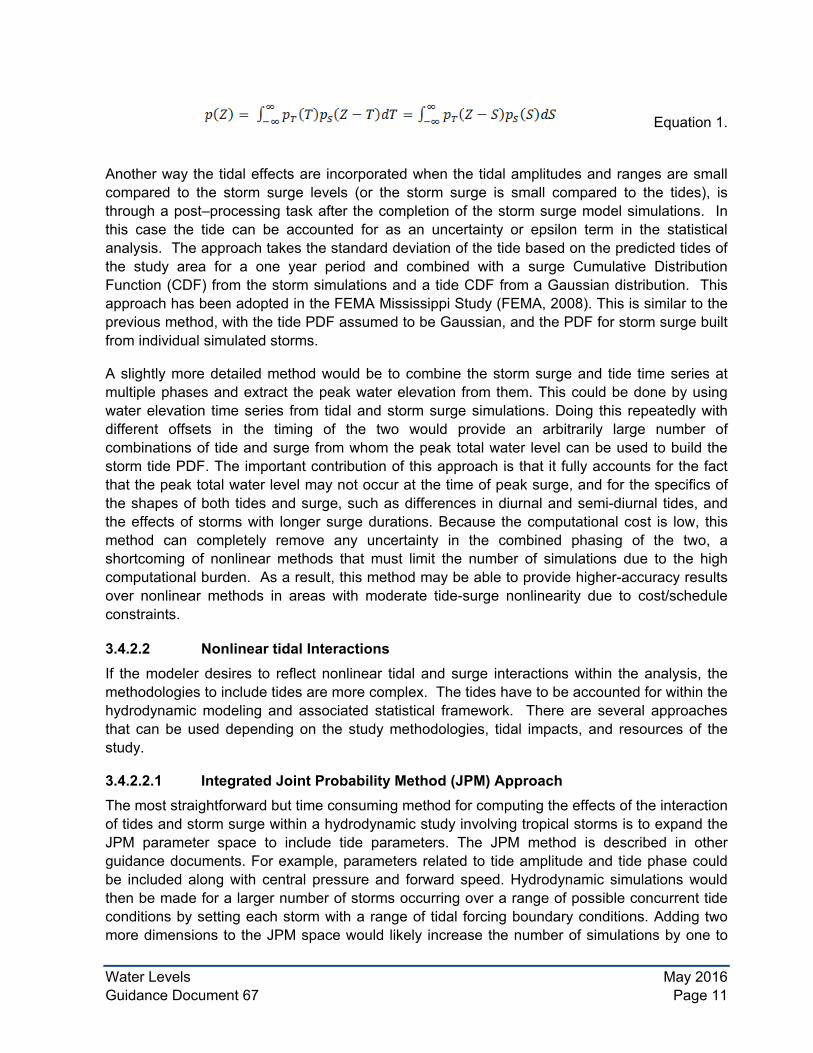
A third, slightly more complex approach still assuming linear interactions and assuming that the tide and total storm surge peak are physically independent, is based on a convolution method. In this method, the PDFs for both tide and storm surge only are used. If the probability density of the tide level Z is denoted by pT(Z) and the probability density of the total surge level is pS(Z), and S and T are dummy variables of integration, then the probability density of the sum of the two is given by Equation 1 where the indicated integrations are over all tide and total surge levels.


Equation 1.

Another way the tidal effects are incorporated when the tidal amplitudes and ranges are small compared to the storm surge levels (or the storm surge is small compared to the tides), is through a post–processing task after the completion of the storm surge model simulations. In this case the tide can be accounted for as an uncertainty or epsilon term in the statistical analysis. The approach takes the standard deviation of the tide based on the predicted tides of the study area for a one year period and combined with a surge Cumulative Distribution Function (CDF) from the storm simulations and a tide CDF from a Gaussian distribution. This approach has been adopted in the FEMA Mississippi Study (FEMA, 2008). This is similar to the previous method, with the tide PDF assumed to be Gaussian, and the PDF for storm surge built from individual simulated storms.

A slightly more detailed method would be to combine the storm surge and tide time series at multiple phases and extract the peak water elevation from them. This could be done by using water elevation time series from tidal and storm surge simulations. Doing this repeatedly with different offsets in the timing of the two would provide an arbitrarily large number of combinations of tide and surge from whom the peak total water level can be used to build the storm tide PDF. The important contribution of this approach is that it fully accounts for the fact that the peak total water level may not occur at the time of peak surge, and for the specifics of the shapes of both tides and surge, such as differences in diurnal and semi-diurnal tides, and the effects of storms with longer surge durations. Because the computational cost is low, this method can completely remove any uncertainty in the combined phasing of the two, a shortcoming of nonlinear methods that must limit the number of simulations due to the high computational burden. As a result, this method may be able to provide higher-accuracy results over nonlinear methods in areas with moderate tide-surge nonlinearity due to cost/schedule constraints.

3.4.2.2 Nonlinear tidal Interactions If the modeler desires to reflect nonlinear tidal and surge interactions within the analysis, the methodologies to include tides are more complex. The tides have to be accounted for within the hydrodynamic modeling and associated statistical framework. There are several approaches that can be used depending on the study methodologies, tidal impacts, and resources of the study.

3.4.2.2.1 Integrated Joint Probability Method (JPM) Approach The most straightforward but time consuming method for computing the effects of the interaction of tides and storm surge within a hydrodynamic study involving tropical storms is to expand the JPM parameter space to include tide parameters. The JPM method is described in other guidance documents. For example, parameters related to tide amplitude and tide phase could be included along with central pressure and forward speed. Hydrodynamic simulations would then be made for a larger number of storms occurring over a range of possible concurrent tide conditions by setting each storm with a range of tidal forcing boundary conditions. Adding two more dimensions to the JPM space would likely increase the number of simulations by one to


two orders of magnitude. Recent JPM work has had storm populations in the 1,000s to 10,000s for studies covering several counties, meaning this approach may be prohibitively expensive. A JPM-Optimum Sampling (JPM-OS) approach should be able to limit the increased computational cost. However, it could still increase the total number of model runs by an order of magnitude.

3.4.2.2.2 Regression Approach The regression approach was used with many FEMA coastal studies completed in the 1980s using the FEMA storm surge model. The approach is fully documented in the FEMA Coastal Storm Surge Model documentation (FEMA, 1988). It involves a set of secondary calculations to be performed following the basic JPM storm simulations. The idea is to perform linear superposition of the simulated JPM storm surge elevations (not including tides) with tides of varying amplitudes and phases, producing a set of added SWL results. A number of additional storm simulations are then run with the various tide amplitudes and phases. In these runs, the tides and the surge are computed together, so that the SWLs represent the fully combined results, not just the simply added results.

At a given grid point, the combined SWLs can be plotted against the added SWLs, to obtain a regression expression relating one to the other. Both tides and storms must be chosen carefully for this exercise in order to cover the ranges of parameters of importance. The result is an approximation that is used to adjust the linear superposition (or “added”) SWLs using computed nonlinear effects. The earlier FEMA documentation recommends the use of different corrections for low and high tide. In addition, preliminary calculations performed for a South Carolina surge study suggested that these corrections may depend on the coordinates and characteristics of the grid point as well as its location relative to the hurricane track. Given these complicated dependencies, this approach is not preferred when nonlinear tidal effects are large and when other approaches can achieve a reasonable level of accuracy.

3.4.2.2.3 Random Timing Approach This approach has been used extensively by the State of Florida in its determinations of Coastal Construction Control Lines (Chiu and Dean, 2002). The State of Florida work was published in a series of county-by-county reports by the Florida Department of Natural Resources (DNR), Bureau of Beaches and Shores. The approach is simple and has been adopted by several recent FEMA studies at the time of this writing, including the FEMA Region II study for New York City and New Jersey (RAMPP, 2014) and the FEMA Region IV study for Georgia and Northeast Florida (BakerAECOM, 2012). The Florida DNR coastal setback work involves Monte Carlo simulations of many hundreds or thousands of storms using an inexpensive 1D surge model (locally calibrated against a 2D model). To account for the effects of tide, the 1D simulations are performed using local tide history as defined by choosing a random starting time in the tide predictions for the hurricane season. Each simulation is performed with a random tide in this way, and the large number of simulations effectively reproduces a very long period of history, with tide and surge appropriately combined. From these simulations, the final SWLs are obtained directly, without need for additional tide analysis. For the studies completed by the Florida DNR, the nature of the Monte Carlo Simulation was applied to a large number of storm simulations, which resulted in a representation of the entire tidal in the model results. Recent FEMA studies using this approach have not used a large number of Monte Carlo simulations,


but instead have assumed that a single random timing assigned to a smaller set of JPM-OS storms can sufficiently capture tide-surge variations. In the case of extratropical storms, such as in the FEMA Region II study, two instances of each storm were simulated, with the second realization of each storm performed at the opposite tide phase of the first.

For each storm simulation, a random starting time within the storm season is selected, and each storm is run with the corresponding tidal parameters. With the JPM, and particularly with a JPM-OS methodology, the Mapping Partner should investigate if the number of storms in the simulation set is sufficient so that the randomly chosen tides adequately sample the significant range of tidal effects in order to produce a stable estimate of the SWL. It may be necessary to simulate each JPM storm with multiple randomly selected tidal start times in order to provide a greater sampling of storm tide possibilities. For extratropical storms where the statistics are fed by the simulation of historic storms, the number of simulated events is limited. Therefore multiple random time scenarios are needed for each storm simulated. Another option for both tropical and extratropical storms would be to only simulate certain storms that are considered particularly important at multiple tides.

3.4.2.2.4 Hybrid - Random Timing Approach If simulating all storms needed for the frequency analysis with tidal effects is not possible due to time and resource constraints, a hybrid approach to the Random Timing Approach is possible. In the hybrid approach, a reduced training set of storms is simulated with and without tidal effects. This is similar to the regression approach except that the simulated training set of storms is chosen randomly throughout the tidal cycle as opposed to at selected highs and lows. This training set is used to develop nonlinear tidal adjustment factors throughout the domain. The adjustment factors are then added to the storm surge simulation peak water level responses along with the sampled tidal elevations. The key to this approach is to simulate enough storms with tides where the storm surge peak occurs at enough points in the tidal range to validate the adjustment factors. As mentioned previously, several factors can affect the level of nonlinearity seen in a study area.

3.5 Wind Drag and Bottom Drag The surface stress distribution resulting from storm induced wind is computed through application of some specified wind drag formulation that includes empirical coefficients. Selection of an appropriate formula and coefficients is extremely important because the shear stress is proportional to the square of the wind speed. A formulation or coefficient that is appropriate for extratropical events may not be appropriate for tropical storms. Additionally, an upper bound to the wind stress may need to be determined due to reduction in sea surface roughness during extreme events. A versatile numerical model should provide the user with capability to specify parameters for a given formulation, including reductions due to the presence of vegetation.

The bottom drag must also be specified. As for the surface shear stress, a versatile numerical model should allow the user a variety of friction options. These options should include linear or quadratic options as well as provisions for variable resistance to account for the effects of all manner of vegetation and structures which might be encountered in overland flood propagation.


3.6 Land Cover Data Land cover type data bases, such as those developed by the USGS or NOAA, can be used to specify the friction resistance characteristics of different portions of the model mesh domain. This can be done in order to maximize the accuracy with which landscapes of various types influence the propagation of the storm surge into an inundated floodplain. Frictional effects of the landscape can be important if the inundated flood plain is large in extent or if the storm surge wave must propagate a significant distance to reach a particular location.

3.7 Wave Setup The application of a basin-wide coupled 2D wave and surge model results in a MWL (SWL plus static wave setup) and it may not be necessary to compute wave setup outside the basin-wide modeling effort. However, this is only the case if sufficient resolution is adopted in the surf zone to compute wave setup accurately for all storms. Wave radiation stress forcing can be included in the numerical model if wave setup is of concern. Further discussion on wave setup can be found in the Wave Setup Guidance document.

3.8 Storm Climatology The historical storm record is needed for two purposes: first, for definition of the characteristics of particular historical storms necessary for hindcast modeling and model validation as discussed above; second, for estimation of storm frequency and frequencies of such storm parameters as may be needed in the statistical simulation effort.

As already noted, extratropical data may be obtained from knowledgeable and experienced Federal agencies, as well as from commercial sources. Similar data for tropical storms and hurricanes is also available. The latter data is more problematic, however, owing to the sporadic quality of hurricanes and to their relatively large spatial gradients in winds and surge (compared with area-wide northeasters, for example). Important northeasters are of such dimension and duration as to affect large coastal areas, including numerous tide gages, and do not generally result in loss of gage data as is often the case for major hurricanes. Consequently, difficulties and limitations of storm climatology are more acute for tropical storms and hurricanes than for extratropical systems. Critical data for historical storms and model validation studies should be prepared by experienced meteorologists.

3.9 Measured Water Level Data Measured water levels are an important data source for coastal flood analyses in many locations.

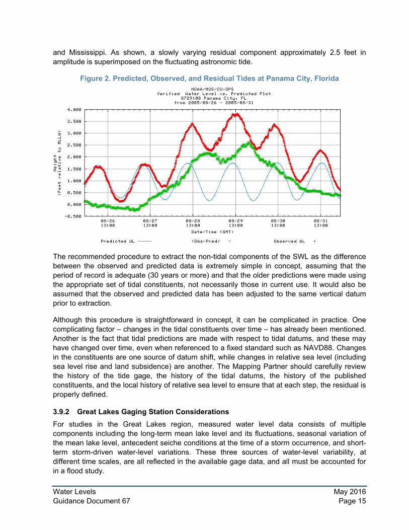
3.9.1 Extraction of Non-astronomic Water Levels from Gage Records Both observed data and a method to predict the purely astronomic component of those observations are available. By subtracting the predictions from the observations, one arrives at a time series of the non-astronomic contribution to the measured SWL (the tide residual or tide anomaly), including surge and meteorological effects, rainfall runoff. Figure 2 shows observed, predicted, and tide residuals (observed minus predicted) at Panama City, Florida for a five-day period in August 2005 during Hurricane Katrina’s approach and landfall to the west in Louisiana


and Mississippi. As shown, a slowly varying residual component approximately 2.5 feet in amplitude is superimposed on the fluctuating astronomic tide.

Figure 2. Predicted, Observed, and Residual Tides at Panama City, Florida

The recommended procedure to extract the non-tidal components of the SWL as the difference between the observed and predicted data is extremely simple in concept, assuming that the period of record is adequate (30 years or more) and that the older predictions were made using the appropriate set of tidal constituents, not necessarily those in current use. It would also be assumed that the observed and predicted data has been adjusted to the same vertical datum prior to extraction.

Although this procedure is straightforward in concept, it can be complicated in practice. One complicating factor – changes in the tidal constituents over time – has already been mentioned. Another is the fact that tidal predictions are made with respect to tidal datums, and these may have changed over time, even when referenced to a fixed standard such as NAVD88. Changes in the constituents are one source of datum shift, while changes in relative sea level (including sea level rise and land subsidence) are another. The Mapping Partner should carefully review the history of the tide gage, the history of the tidal datums, the history of the published constituents, and the local history of relative sea level to ensure that at each step, the residual is properly defined.

3.9.2 Great Lakes Gaging Station Considerations For studies in the Great Lakes region, measured water level data consists of multiple components including the long-term mean lake level and its fluctuations, seasonal variation of the mean lake level, antecedent seiche conditions at the time of a storm occurrence, and short-term storm-driven water-level variations. These three sources of water-level variability, at different time scales, are all reflected in the available gage data, and all must be accounted for in a flood study.


For the Great Lakes, many water-level gaging stations are in operation and report levels hourly. Some gages have been in existence for very long periods of time and hourly data acquired since the 1970s are readily available; hourly data acquired prior to 1970 less so. Monthly maxima and monthly mean data are readily available and are very useful for evaluating long-term trends in lake levels. The utility of the monthly maxima and monthly means for estimating historical storm surges has varied from lake to lake (Melby et al., 2012 and Baird, 2012). These data are available from the NOAA and USACE. NOAA provides access to its data through NOAA’s National Water Level Observation Network (NWLON) database. The USACE, Detroit District, provides water-level data on its web site. Other sources of water-level data may also be available in particular locations, and these should be sought by the Mapping Partner as part of the study scoping effort.

Long-term lake level changes are a result of both the natural processes mentioned above and anthropogenic activities. The long-term lake level variability is assumed to be a stationary process over the past 50 years. Further, the findings of Baedke and Thompson (2000) indicate the level of Lake Michigan has been stable for over 3,000 years. This is important in the consideration of water-level probabilities and must be evaluated for each lake.

Adjustment values to account for changes in lake conditions and water-control operations over time due to anthropogenic activities such as channel deepening, water diversion, or water management regulations are applied to mean monthly lake levels derived from NOAA water-level measurements in order to estimate lake levels that would have existed historically had the lakes been operated under current regulations and physical conditions. These modifications, called the Basis of Comparison (BOC) adjustments, were developed as a product from the International Joint Commission (IJC) Levels Reference Study in 1993 and then more recently in 2003. The modified mean monthly lake levels are adopted in these guidelines to characterize the current state of both the expected range and variability in long-term and seasonal-scale lake level changes.

In general, FIS are intended to be based on existing conditions. Strictly speaking, then, a study could ignore long term variability, adopting the current mean annual level for the analysis. However, the data shows that significant variability can occur over a period of just a few years, and it is recognized that both flood maps and new construction have lifetimes during which such variations may be significant. Therefore, long term variability should be accounted for in the analyses.

3.10 Ice Cover Storm surge modeling on the Great Lakes also requires ice fields as input. Using ice fields developed from data sources such as NOAA’s Great Lakes Environmental Research Laboratory (GLERL), the effective wind stress applied to the water surface in the surge modeling can be influenced by the concentration of the ice and by the horizontal extent of ice cover.

An additional physical process that has been examined in ice-covered regions such as the Great Lakes is the influence of sea ice as a source of aerodynamic roughness. Many storm surge models use the wind drag coefficient formulation of Garratt (1977) in the calculation of surface wind stresses. This is a widely-used formulation and it has been found to work well for storm surge applications. Macklin (1983) and Pease et al. (1983) found that measurements


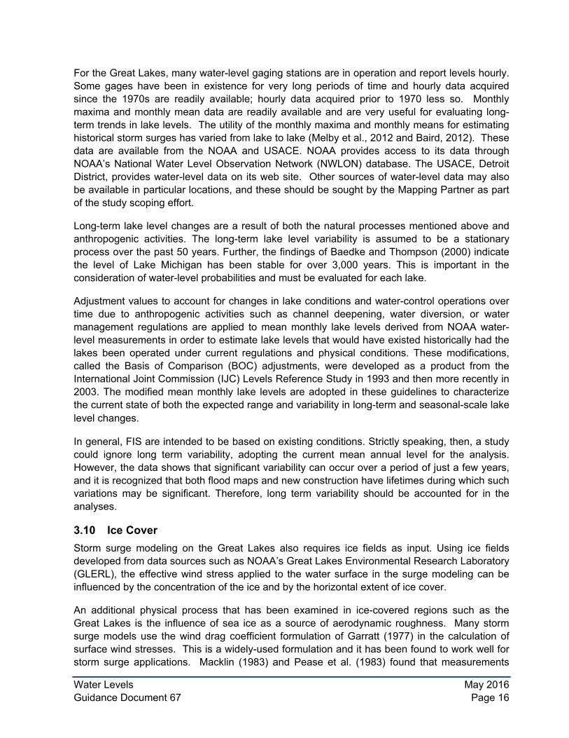
over first year sea ice typically yielded wind drag coefficient values that were significantly larger, and varied less with wind speed, than that those predicted for open water. More recent work (Birnbaum and Lupkes, 2002, and Garbrecht et al., 2002) formalized the effect of form drag associated with ice on the specification of wind drag coefficients within marginal ice zones. From their work, Chapman et al. (2005 and 2009) utilized an empirical fit to the range of field data for the air-ice-water effective wind drag coefficient, CDF, and suggested in Equation 2 in which IC is the ice concentration varying from 0.0 to 1.0 (corresponding to 0 percent to 100 percent) for open water and complete ice cover conditions, respectively.

Equation 2.

Inspection of this air-ice-water-wind drag coefficient formula shows that a maximum value of 0.0025 occurs with 50-percent ice coverage. This value is very close to the Macklin (1983) measurement of 0.0028 for first year ice. Furthermore, it is seen that the value of the drag coefficient is symmetrical at about 50-percent ice coverage suggesting that the drag coefficient needed to represent 75-percent ice coverage is close to that of 25-percent ice coverage. An alternative linear fit dependence on ice concentration has been applied by Danard et al. (1989). These notions regarding variation of wind drag coefficient with ice cover have been supported by a number of Chukchi and Beaufort Sea storm surge simulations (Henry and Heaps, 1976; Kowalik, 1984; and Schafer, 1966) in which, wind drag coefficients greater than or equal to 0.0025 where utilized. The interactions of wind, ice, and the water column are not well understood, however. Testing and validation of the approach for treating ice cover in the modeling is recommended where possible.

If ice cover is present and the increased drag coefficient, calculated with Equation 2, exceeds the value calculated using the standard Garratt (1997) formulation, it is recommended to replace the standard Garratt wind drag coefficient with the increased value associated with the presence of ice cover.

3.11 Model Validation Validation of the hydrodynamic model is critical to ensure that mesh resolution, bathymetry, topography, and boundary conditions are adequately defined. Validation includes elements commonly thought of as calibration, although, in general, surge models should not be calibrated in a traditional sense to reproduce observations. Fundamental model parameters such as wind stress coefficients, overland friction factors, and the like, should be based on published best-estimates, and are not free parameters for calibration.

For tides, validation can be achieved by comparing computed data to either measured data collected for a specific time period at the location of interest, or to a multi-constituent (i.e., M2, S2, N2, N1, K1, O1, Q1, and P1) tidal time series reconstructed from published harmonic constituents. These constituents are available from the tidal data base sources such as the NOS or the International Hydrographic Center (IHC). Tidal validation should be achieved to better than 10 percent in both amplitude variation throughout the domain, and phase variation; generally, even better results should be possible. Failure to achieve tidal validation might indicate inadequate mesh resolution, especially at inlets and other critical points. Failure to achieve tidal validation should be documented. Any subsequent model calibration efforts to


adjust bottom friction should be limited to values within published ranges for the local hydraulic conditions.

Validation for storm events is more complex. In order to achieve a meaningful result, both the storm conditions (winds and pressures) and the response conditions (such as gage data and high-water marks) must be known with accuracy. This is seldom achieved. Actual storm winds and pressures do not faithfully follow simple models, for example, and observed high-water marks may be contaminated by very local wave effects, and may include varying proportions of the local wave setup. Tide and wave gage observations are more reliable, although, again, it is necessary to assess to what degree the record might incorporate setup; it also often happens that tide gages fail prior to the surge peaks of major storms.

In any case, the Mapping Partner may undertake a thorough validation/hindcast effort for all significant storms that have affected the study area for which high quality data are available. Special hydrodynamic simulations using wind and pressure estimates are required; such wind and pressure data may be available from Federal agencies, or may be obtained from commercial sources specializing in meteorological data. High-water marks and tide and wave gage records must be evaluated to account for the possible contributions of setup and runup. It should not be expected that an exact comparison will be achieved for any storm. However, given several storms, the observed data should scatter around the model simulations, and not show any large, consistent bias. Deviations from generally acceptable validation should be discussed in the study documentation. If certain areas of the mesh produce consistently poor comparisons, this may suggest that the mesh definition should be carefully reviewed to ensure that area-wide features, such as elongated road embankments, have been accounted for. Of course, it is also important to ensure that the mesh represents conditions which prevailed at the time of the storm; barrier island erosion or inlet alterations from prior storms may produce sizeable alterations in a simulation. Consequently, it may be necessary to develop different mesh versions for hindcasts, in order to obtain valid results.

For the Great Lakes, in particular, various parts of a lake respond differently to any one particular storm, and the storm that produces extreme water levels in one part of the lake might not, and probably does not, produce extreme levels in other parts. For all studies, the number of validation storms must be large enough to assess model prediction skill along all parts of the shoreline that are to be mapped. Measured water-level data are used to perform the validation, through comparisons between measured and modeled water levels. To the extent possible, the treatment of ice should be validated by appropriate selection of validation storms.

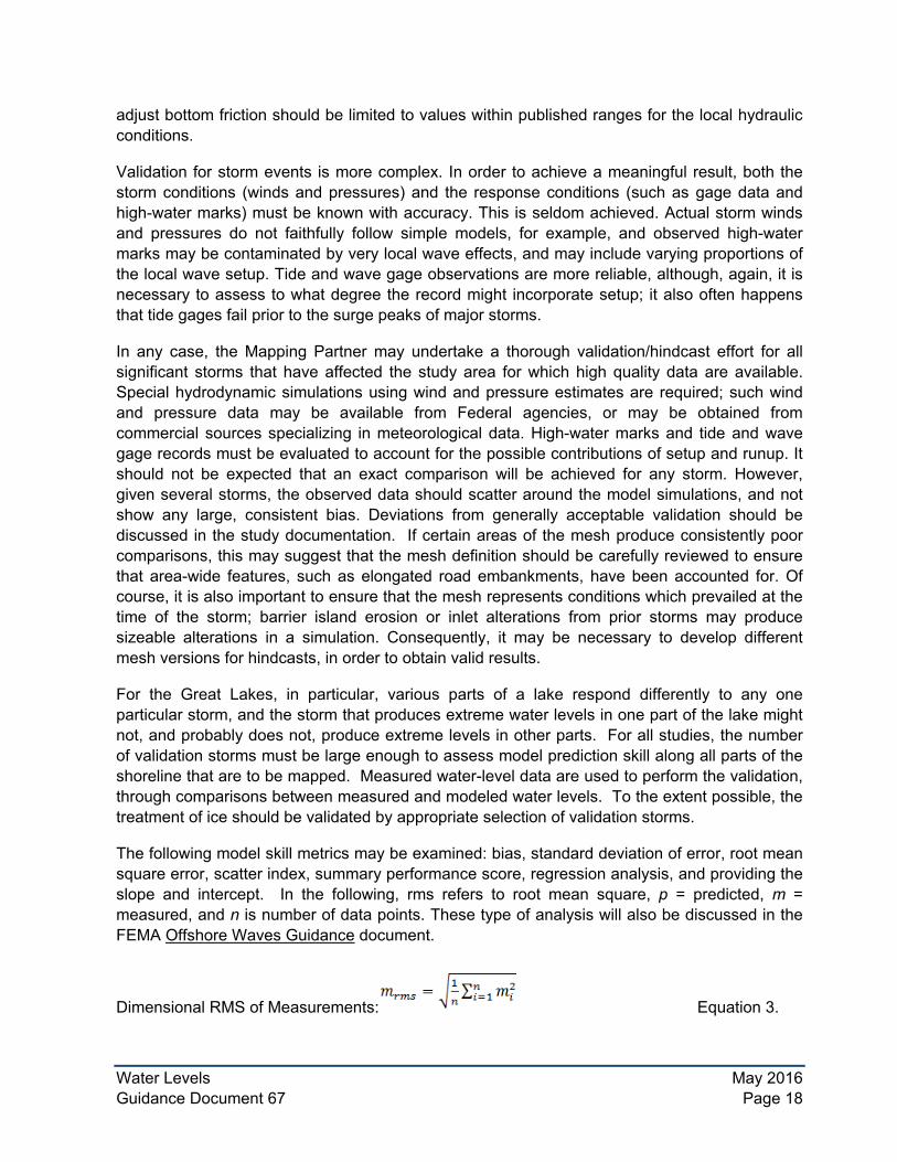
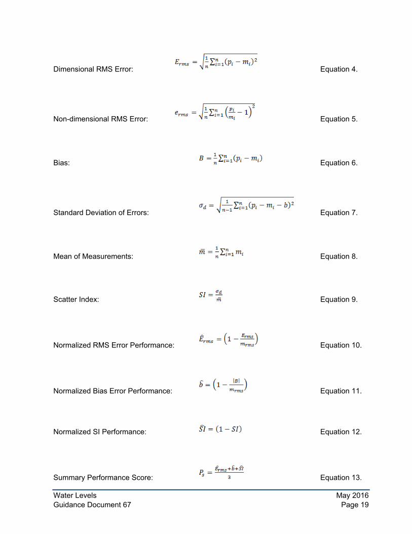
The following model skill metrics may be examined: bias, standard deviation of error, root mean square error, scatter index, summary performance score, regression analysis, and providing the slope and intercept. In the following, rms refers to root mean square, p = predicted, m = measured, and n is number of data points. These type of analysis will also be discussed in the FEMA Offshore Waves Guidance document.

Dimensional RMS of Measurements: Equation 3.


Dimensional RMS Error: Equation 4.

Non-dimensional RMS Error: Equation 5.

Bias: Equation 6.

Standard Deviation of Errors: Equation 7.

Mean of Measurements: Equation 8.

Scatter Index: Equation 9.

Normalized RMS Error Performance: Equation 10.

Normalized Bias Error Performance: Equation 11.

Normalized SI Performance: Equation 12.

Summary Performance Score: Equation 13.


Should the validation effort be inconclusive, or should poor results be consistently obtained for the historical storm set, the Mapping Partner shall confer with the FEMA Study Representative and with FEMA’s technical representatives in order to resolve the issue prior to proceeding with further modeling.

4.0 Water Levels in Sheltered Waters Water levels in sheltered waters may be influenced by a variety of factors that can alter coastal flood characteristics. Incoming storm surge and the resulting extreme SWLs along the shorelines of sheltered waters may achieve higher elevations than at adjacent open-coast locations owing to channelization and tidal amplification controlled by the orientation, geometry, and bathymetry of the basin; lower elevations may occur if restrictive tidal inlets impede the incoming tide. Factors such as these should be implicitly accounted for in any detailed 2D storm-surge modeling, and so would not need special attention. However, small basins may also experience higher water levels from the contributions of other mechanisms such as direct precipitation and runoff, or from resonant basin oscillations called seiche. These are non-standard factors in a FEMA coastal study, but should be considered by the Mapping Partner if the initial scoping effort suggests that there is reason to believe that the local conditions are such that a special problem or sensitivity might exist.

For studies based not on a detailed 2D model but on, for example, tide gage analysis, recorded tide elevations may require transposition from the tide gage to a nearby flood study site within the sheltered waters, to better represent the local SWL during the 1-percent-annual-chance flood event. Some general guidance for evaluating and applying tide gage data to ungaged locations is provided in Section 4.1, although the Mapping Partner must carefully assess the likely magnitude of error inherent in such approximations, and determine whether a more detailed study might be necessary.

4.1 Variability of Tide and Storm Surge in Sheltered Waters As a very long wave such as storm surge or tide propagates though a varying geometry, its amplitude changes in response to reflection, frictional damping, variations in depth causing shoaling, and variations in channel width causing convergence or divergence of the wave energy.

In some cases, tide data may have to be transposed from a gaged site to an ungaged site. If a sheltered water study site is located in the immediate vicinity of a tide gage, the Mapping Partner can use data from the gage without adjustments, but if the study site is distant from the tide gage, the tide data may need to be adjusted so as to reasonably represent the site. It is emphasized that “Considerable care must be exercised in transposing the adjusted observed [tide] data to a nearby site since large discrepancies may result” (USACE, 1986).

Some simple empirical evidence may permit an approximate evaluation of these variations, adequate for a FIS:


• Established tidal datums from multiple gages in the sheltered area reflect the natural variation of tide elevations; interpolation between gages gives a first-order estimate of spatial variation patterns

• The normal vegetation line may provide additional information between gages, insofar as it mirrors the general variation of the normal tidal elevation.

• Similarly, observed debris lines and high-water marks from historical storms may illustrate the variation of storm surge within the sheltered geometry, outside the surge generation zone.

The Mapping Partner must evaluate the differences between the physical settings of the nearest tide gage(s) and the study site, and the distance and hydraulic characteristics of the intervening waterways between these locations to establish a qualitative understanding of the potential differences in tidal elevations between the gaged and ungaged locations. If flood high-water marks are available in the vicinity of the ungaged sheltered water study site, these elevations may be compared to recorded tide elevations to correlate storm surge components of the SWL between locations. In general, storm surge data are of more limited availability than tide data. It may sometimes be reasonable to assume similarity between storm surge and tide, and so infer surge variation from known tide variation. The validity of such inference is limited, however, by differences in amplitude and duration of high water from the two processes, and by the fact that tide is cyclic and so may not vary in the same manner as a single surge wave.

Both empirical equations and numerical models can be used to describe the variation of tides and storm surges propagating into sheltered water areas. The Mapping Partner may select the most appropriate approach for the study, with consideration of the location of the study site within the sheltered water body, the complexity of the physical processes, and the cost of a particular approach. Appropriate numerical models can range from simple 1D models to complex 2D models. The Mapping Partner may thoroughly evaluate the limitations and capabilities of appropriate models in view of the site-specific issues that need to be resolved to obtain reliable estimates of tidal flood elevations.

Tidal inlets control the movement of water between the open coast and adjacent sheltered waters. Inlets may be broadly classified as unimproved (natural) or improved (maintained). The physical opening of a tidal inlet, whether natural or maintained, has a direct and often significant effect on the propagation of tides, storm surge, and waves into sheltered waters and on subsequent coastal flood conditions. For simple tidal inlet settings, or as a first approximation before detailed numerical modeling, Mapping Partners may use analytical methods to estimate bay tide amplitudes. These analytical methods may also be applied in a two-step process to transpose recorded tide gage data from one bay to another nearby ungaged sheltered water body as follows:

1. Apply the analytical methods in reverse to estimate the adjacent open-coast annual maximum SWLs based on recorded SWLs from a primary tide gage in the sheltered water body closest to the flood study site. The physical setting of a primary tide gage may be such that recorded tide elevations are representative of open-coast tide elevations; however, this condition should not be assumed.


2. Using the estimated open-coast tide elevation, reapply the analytical methods andnomograms (in forward mode) to estimate the associated annual maximum SWLs in theungaged sheltered water body where the study site is located. Use of the same open-coast stillwater elevation between the gaged and ungaged sheltered water areas isacceptable if it can be assumed that the annual extreme SWLs are generated fromregional storm systems large enough in spatial extent to encompass the two locations.

Irrespective of the approach taken, the Mapping Partner may evaluate the physical setting of the tide gage(s) from which data are used. Observation of the gage setting may provide insight into the relative degree of sheltering or other characteristics of a given tide gage

If the physical setting and tidal processes of a coastal flood study site are particularly complex, the Mapping Partner must confer with the FEMA Study Representative and technical representatives for further guidance on estimating tidal and storm surge elevations at ungaged sites.

4.2 Seiche Seiche is a low frequency oscillation occurring in enclosed or semi-enclosed basins, which may be generated by incident waves or atmospheric pressure fluctuations; seiching may also be called harbor oscillation, harbor resonance, surging, sloshing, and resonant oscillation. It is usually characterized by wave periods ranging from 30 seconds to 10 minutes, controlled by the characteristic dimensions and depth of the basin (USACE, 2003).

The amplitude of seiche is usually small; the primary concern is often with the associated currents that can cause large excursions and damage to moored vessels if resonance occurs. However, surface elevations and boundary flooding in an enclosed basin may become pronounced if the incoming wave excitation contains significant energy at the basin’s natural seiche periods. The Mapping Partner may investigate the likelihood of seiche under extreme water-level and wave conditions if the pre-project scoping effort indicates that a sensitive site has been affected by seiche during past storms. Bathymetry, basin dimensions, and incoming wave characteristics should be reviewed to determine the potential for seiching. Numerical models may be appropriate for evaluating the effects of long waves in enclosed basins and may be considered for use in a sheltered water study if seiching is believed to have the potential to contribute significantly to boundary flooding during the 1-percent-annual-chance flood condition.

4.3 Estimating Sheltered Water Levels Using Existing Flood Insurance Study Data Unlike a new detailed coastal study in a sheltered water area, previous modeling for an existing FIS may not account explicitly for all SWL parameters. Thus, the following issues should be considered when updating an existing study:

Inland Penetration of the Coastal Flood – If a sheltered basin is included within the domain of a detailed coastal study, the coastal influence will be explicitly included. However, if a basin falls outside the detailed study region, but is hydraulically connected to the coast during flooding, then the coastal influence must be routed to the site. Although the 1-percent-annual-chance stillwater elevation is a statistical entity and not associated with any particular storm, the Mapping Partner may be able to approximate the coastal influence by use of an equivalent-


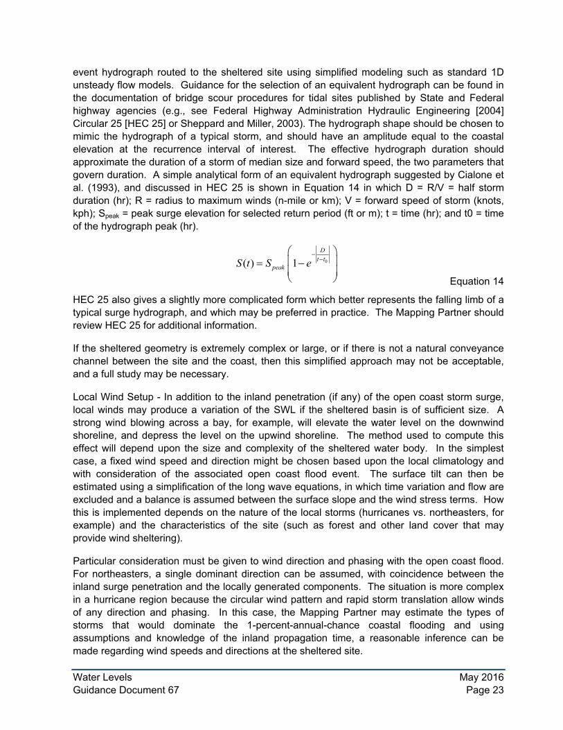
event hydrograph routed to the sheltered site using simplified modeling such as standard 1D unsteady flow models. Guidance for the selection of an equivalent hydrograph can be found in the documentation of bridge scour procedures for tidal sites published by State and Federal highway agencies (e.g., see Federal Highway Administration Hydraulic Engineering [2004] Circular 25 [HEC 25] or Sheppard and Miller, 2003). The hydrograph shape should be chosen to mimic the hydrograph of a typical storm, and should have an amplitude equal to the coastal elevation at the recurrence interval of interest. The effective hydrograph duration should approximate the duration of a storm of median size and forward speed, the two parameters that govern duration. A simple analytical form of an equivalent hydrograph suggested by Cialone et al. (1993), and discussed in HEC 25 is shown in Equation 14 in which D = R/V = half storm duration (hr); R = radius to maximum winds (n-mile or km); V = forward speed of storm (knots, kph); Speak = peak surge elevation for selected return period (ft or m); t = time (hr); and t0 = time of the hydrograph peak (hr).

Equation 14

D−

S t( ) = S 1 t t0peak − e −

HEC 25 also gives a slightly more complicated form which better represents the falling limb of a typical surge hydrograph, and which may be preferred in practice. The Mapping Partner should review HEC 25 for additional information.

If the sheltered geometry is extremely complex or large, or if there is not a natural conveyance channel between the site and the coast, then this simplified approach may not be acceptable, and a full study may be necessary.

Local Wind Setup - In addition to the inland penetration (if any) of the open coast storm surge, local winds may produce a variation of the SWL if the sheltered basin is of sufficient size. A strong wind blowing across a bay, for example, will elevate the water level on the downwind shoreline, and depress the level on the upwind shoreline. The method used to compute this effect will depend upon the size and complexity of the sheltered water body. In the simplest case, a fixed wind speed and direction might be chosen based upon the local climatology and with consideration of the associated open coast flood event. The surface tilt can then be estimated using a simplification of the long wave equations, in which time variation and flow are excluded and a balance is assumed between the surface slope and the wind stress terms. How this is implemented depends on the nature of the local storms (hurricanes vs. northeasters, for example) and the characteristics of the site (such as forest and other land cover that may provide wind sheltering).

Particular consideration must be given to wind direction and phasing with the open coast flood. For northeasters, a single dominant direction can be assumed, with coincidence between the inland surge penetration and the locally generated components. The situation is more complex in a hurricane region because the circular wind pattern and rapid storm translation allow winds of any direction and phasing. In this case, the Mapping Partner may estimate the types of storms that would dominate the 1-percent-annual-chance coastal flooding and using assumptions and knowledge of the inland propagation time, a reasonable inference can be made regarding wind speeds and directions at the sheltered site.


Rainfall Contributions - Open coast flood levels are primarily controlled by surge and tide, neglecting any rainfall contribution. However, the relative significance of rain may increase in sheltered waters where the surge/tide magnitude declines and where the rain volume is concentrated and confined within the local watershed. In order to account for rainfall effects, the Mapping Partner may adopt a rainfall representative of the local storm characteristics (e.g., hurricane or northeaster), and estimate the runoff within the sheltered watershed as an addition to the surge prism. Owing to a lack of hurricane rainfall data and the complexity of the combined processes, a simple approach to rainfall selection is recommended. For hurricanes, an empirical estimate of rainfall intensity vs. central pressure and radius was developed for the Interagency Performance Evaluation Task Force (IPET) study (Fredrickson, et. al, 2007) based on the National Aeronautics and Space Administration (NASA) Tropical Rainfall Measuring Mission. The suggested intensity in millimeters per hour for radial distances r (n-mile) from the eye is given by Equation 15.

Equation 15. ( )

>∆+

≤∆+=

−−max

/3.0max

;)12.014.1(

;)12.014.1()(

maxmax RrePk

RrPkrm RRr

In this equation, Rmax is the radius to maximum winds (n-mile), ∆P is the central pressure deficit in millibars, and k is a dimensionless coefficient accounting for azimuthal variation. Following the IPET study, it is suggested that k be taken as 1.0 to the left of the eye, and 1.5 to the right (for Atlantic Ocean and Gulf of Mexico studies).

When implemented as an equivalent single storm, suitable values for the storm parameters are the median local radius and the pressure corresponding to a storm producing a peak coastal surge approximating the 1-percent-annual-chance value. An analogous approach could be followed for northeasters, with the additional option of basing the rainfall estimate directly on historical rainfall observations (averaged over multiple gages) for storms that produced coastal levels approximating the 1-percent-annual-chance value.

5.0 Nonstationary Processes Conceptually, a stationary process may be thought of as one that does not change in its essential characteristics over time; its descriptors are fixed or stationary. For example, a stationary random process would be one for which its mean, standard deviation, and other moments are unchanging over time. A nonstationary process is one for which these measures do change. Whether a fluctuating process is thought to be, or appears to be, nonstationary can depend upon the time window through which it is viewed. Processes that appear to display definite nonstationary trends when viewed at a short scale, may be seen to fluctuate around an unchanging mean when viewed from a more distant perspective. For example, the tide appears nonstationary when viewed over a period of one hour, but appears entirely stationary when viewed over an entire 19 year tidal epoch.

For practical FIS considerations, two sorts of nonstationarity seem significant. The first is the apparent change of sea level, which has been observed on all coasts. Because it is sea level


relative to land that is most significant, an apparent change of sea level can be the result of either sea level rise, or land subsidence.

The second type of nonstationarity that is important for coastal studies is the long-term change in tidal datums, which may occur as basins evolve through silting, dredging, migration and evolution of inlets, human construction including harbor improvements and breakwaters, and so forth. Both types are discussed below.

5.1 Relative Sea Level – Sea Level Rise Sea level rise appears to be a real, long-term effect observed all along the U.S. Ocean and Gulf of Mexico coastlines. Sea level trend data for individual stations along the Atlantic Ocean, Gulf of Mexico, and Pacific Ocean coasts can be obtained from NOAA’s website, http://tidesandcurrents.noaa.gov/sltrends/sltrends.shtml. The Mapping Partner must be aware of these changes to properly interpret historical data upon which new studies might be partly based. This has been discussed in Section 2.0 of this guidance document.

5.2 Relative Sea Level – Land Subsidence and Rebound Land subsidence produces the same sort of effect as sea level change – a rise in the apparent sea level – but subsidence might be the more significant factor in a local area. Many areas along the coasts of Texas, Louisiana, Mississippi, and Southern California have subsided by several feet as a result of gas, oil, or water extraction over the past few decades. Some parts of Alaska are experiencing the opposite – land rebound – due to post-glacial isostatic adjustment resulting in net decrease in sea level compared to the land.

Large displacements make it imperative that historical data be interpreted with caution. The Mapping Partner must ensure that gage datums have been properly adjusted over time so that water-level records, benchmarks, observed high-water marks, and all similar data are properly interpreted and properly related to current conditions represented in the hydrodynamic model mesh.

The USGS is a primary repository of land subsidence data for the United States, and should be consulted to obtain local site information covering the entire period of study data that might be compromised by unrecognized subsidence.

Other data sources may be more helpful in some cases. The Mapping Partner should consult with local city and county engineering departments, and the professional surveying community, which may be aware of isolated subsidence issues not reflected in the national programs.

5.3 Astronomic Tide Variation Tide datums and tidal constituents may change over time owing to changes in the geometry of a tidal basin, so that tide may also constitute a nonstationary process. This makes it imperative that tide predictions for prior years (hindcasts) be made using tidal constituents appropriate to that time, and that tidal data be adjusted as necessary for shifts in tidal datums with respect to a fixed datum such as NAVD88 or NGVD29. The NOAA website can provide predictions for past times, but all such predictions are made using the current default set of constituents, and so may inaccurately portray past tide levels and datums. Archived copies of tidal constituents can

http://tidesandcurrents.noaa.gov/sltrends/sltrends.shtml


be obtained from NOAA by special request. Flexibility in applications such as these makes it possible to use a tide prediction.

6.0 References Baird, (2011). FEMA Pilot Studies for Great Lakes Coastal Flood Mapping. Prepared for the USACE Detroit District and FEMA.

BakerAECOM, (2012). JPM-OS Probabilistic Model Development; Intermediate Data Submittal 1, Section 5. Task Order 75: Georgia-Northeast Florida Flood Insurance Study. Submitted to FEMA Region IV.

Baedke, S.J. and Thompson, T.A., (2000). A 4,700-Year Record of Lake Level and Isostasy for Lake Michigan. Journal of Great Lakes Research; 26(4), pp 416-426.

Birnbaum, G. and Lupkes, C., (2002). A new parameterization of surface drag in the marginal sea ice zone, Tellus, 54 A, pp. 107-123.

Chapman, R. S., Mark, D. and Cialone A., (2005). Regional tide and storm-induced water level prediction study for the West Coast Alaska, Draft Report to POA, U.S. Army Engineer Waterways Experiment Station, Vicksburg, MS.

Chapman, R. S., Kim, S-C and Mark, D. J., (2009). Storm-induced water level prediction study for the Western Coast of Alaska. Draft Report to POA, U.S. Army Engineer Waterways Experiment Station, Vicksburg, MS.

Chiu, T.Y, and R.G. Dean (2002). Methodology on Coastal Construction Control Line Establishment. Beaches and Shores Resource Center, Institute of Science and Public Affairs, Florida State University. Retrieved from www.dep.state.fl.us/beaches/publications/pdf/cccl-method/method.pdf (accessed April 20, 2016).

Cialone, M.A., Butler, H.L., and Amein, M., (1993). DYNLET1 Application to Federal Highway Administration Projects, Miscellaneous Paper CERC-93-6, U.S. Army Engineer Waterways Experiment Station.

Danard, M. B., Rasmussen, M. C., Murty, T. S., Henry, R. F., Kowalik, Z., and Venkatesh, S.: 1989, Inclusion of ice cover in a storm surge model for the Beaufort Sea, Natural Hazards 2, 153–171.

Federal Emergency Management Agency (1988). Coastal Flooding; Hurricane Storm Surge Model. Volume 1, Methodology, Office of Risk Assessment, Federal Insurance Administration, Washington DC.

Federal Emergency Management Agency (FEMA) (2008). Mississippi Coastal Analysis Project: Coastal Documentation and Main Engineering Report. Project reports prepared by URS Group Inc., (Gaithersburg, MD and Tallahassee, FL) under HMTAP Contract HSFEHQ-06-D-0162, Task Order 06-J-0018.

Federal Highway Administration, (2004). Tidal Hydrology, Hydraulics and Scour at Bridges, Hydraulic Engineering Circular No. 25, Washington, D.C. Retrieved from http://www.fhwa.dot.gov/engineering/hydraulics/hydrology/hec25.cfm

http://www.dep.state.fl.us/beaches/publications/pdf/cccl-method/method.pdf

http://www.dep.state.fl.us/beaches/publications/pdf/cccl-method/method.pdf

http://www.fhwa.dot.gov/engineering/hydraulics/hydrology/hec25.cfm


Fredrickson, H., Furey, J., Foote, C. and Richmond, M. (2007). Environmental Consequences of the Failure of the New Orleans Levee System During Hurricane Katrina; Microbiological Analysis, ERDC/EL TR-07-7, U.S. Army Engineer Research and Development Center, Vicksburg, MS.

Garbrecht, T., Lupkes, C., Hartmann, J. and Wolff, M. (2002), Atmospheric drag coefficients over sea ice—validation of a parameterization concept, Tellus, 54 A, pp. 205-219.

Garratt, J.R., (1977). Review of drag coefficients over oceans and continents, Monthly Weather Review 105, 915-929.

Henry, R.F. and Heaps, N.S., (1976). Storm surges in the southern Beaufort Sea, Journal Fisheries Research Board Canada, 33, 2362-2376.

Kowalik, Z. (1984). Storm surges is the Beaufort and Chukchi Seas, Journal of Geophysical Research, 89, No. C6, pp. 10,570-10578.

LeProvost, C., Bennett, A.F., and Cartwright, D.E. (1995). Ocean tides for and from TOPEX/POSEIDON, Science, 267, 639-642.

LeProvost, Lyard, F., Molines, J.M., Genco, M.L., and Rabilloud, F. (1998). A hydrodynamic ocean tide model improved by assimilating a satellite altimeter-derived data set, Journal of Geophysical Research, 103, 5513-5529.

Macklin, S.A. (1983). Wind drag coefficient over first‐year sea ice in the Bering Sea. Journal of Geophysical Research, 88.

Melby, J.A., (2012), “Runup Prediction for Flood Hazard Assessment,” U.S. Army Corps of Engineers, TR-XX-12

Mukai, A.Y., Westerink, J.J., and Luettich Jr., R.A., (2002). Guidelines for Using the Eastcoast 2001 Database of Tidal Constituents within the Western North Atlantic Ocean, Gulf of Mexico and Caribbean Sea, Coastal and Hydraulic Engineering Technical Note (IV-XX), 24p.

Pease, C.H., Salo, S.A. and Overland, J.E. (1983). Drag measurements for first-year sea ice over a shallow sea, Journal of Geophysical Research, 88.

RAMPP, 2014, Region II Storm Surge Project - Joint Probability Analysis of Hurricane and Extratropical Flood Hazards, FEMA TO HSFE02-09-J-001, 2013.

Schafer, P. J. (1966). “Computation of storm surge at Barrow, Alaska,” Archiv. Meteorol., Geophys. BioKimatol. Vol. A, No. 15(3-4), pp 372-393.

Schwiderski, E.W., (1980). On charting global ocean tides, Rev. Geophys., 18, 243-268.

Sheppard, D. Max, and William Miller, Jr., 2003. Design Storm Surge Hydrographs for the Florida Coast, Department of Civil and Coastal Engineering, University of Florida, Gainesville. Prepared for the Florida Department of Transportation, Tallahassee, under FDOT Contract BC-354 RWPO 70.

USACE, (1986). Storm Surge Analysis and Design Water Level Determinations, EM 1110-2-1412, DAEN-CWH-W, Washington, D.C., April 15.

USACE, (2003). Coastal Engineering Manual. EM 1110-2-1110, U.S. Army Corps of Engineers, Washington, D.C. (in 6 volumes).

http://acwc.sdp.sirsi.net/client/search/asset/1003142

Guidance for Flood Risk Analysis and Mapping - Home | … · 2016-08-24 · Guidance for Flood Risk...

Documents

Transcript of Guidance for Flood Risk Analysis and Mapping - Home | … · 2016-08-24 · Guidance for Flood Risk...