GUIDANCE, FLIGHT MECHANICS AND TRAJECTORY OPTIMIZATION

NASA CONTRACTOR

REPORT

+- .

i’,, AFWL I WLI L-2) KIRTIAND AFB. N MFY

GUIDANCE, FLIGHT MECHANICS AND TRAJECTORY OPTIMIZATION

Volume XIV - Entry Guidance Equations

by M. B. Tumbiwro und E. F. -3Czmts

Prepared by

NORTH AMERICAN AVIATION, INC.

Downey, Calif.

for George C. Marshall Space Flight Center

NATIONAL AERONAUTICS AND SPACE ADMINISTRATION l WASHINGTON, D. C. . APR’n 1968

.- .- ,. .

TECH LIBRARY KAFB, NM

OOb0425 NASA CR- 1013

GUIDANCE, FLIGHT MECHANICS AND TRAJECTORY OPTIMIZATION

Volume XIV - Entry Guidance Equations

By M. B. Tamburro and E. F. Knotts

Distribution of this report is provided in the interest of information exchange. Responsibility for the contents resides in the author or organization that prepared it.

Issued by Originator as Report No. SID 66- 1678-6

Prepared under Contract No. NAS 8-11495 by NORTH AMERICAN AVIATION, INC.

Downey , C alif.

for George C. Marshall Space Flight Center

NATIONAL AERONAUTICS AND SPACE ADMINISTRATION

For sale by the Clearinghouse for Federal Scientific and Technical Information

Springfield, Virginia 22151 - CFSTI price $3.00

FOREWORD

This report was prepared under contract NAS 8-11495 and is one of a series intended to illustrate analytical methods used in the fields of Guidance, Flight Mechanics, and Trajectory Optimization. Derivations, mechanizations and recommended procedures are given. Below is a complete list of the reports in the series.

Volume I Volume II Volume III Volume IV

Volume V Volume VI

Volume VII Volume VIII Volume IX Volume X Volume XI Volume XII

Volume XIII Volume XIV Volume XV Volume XVI Volume XVII

Coordinate Systems and Time Measure Observation Theory and Sensors The-Two Body Problem The Calculus of Variations and Modern

Applications State Determination and/or Estimation The N-Body Problem and Special Perturbation

Techniques The Pontryagin Maximum Principle Boost Guidance Equations General Perturbations Theory Dynamic Progrsmming Guidance Equations for Orbital Operations Relative Motion, Guidance Equations for

Terminal Rendezvous Numerical Optimization Methods Entry Guidance Equations Application of Optimization Techniques Mission Constraints and Trajectory Interfaces Guidance System Performance Analysis

The work was conducted under the direction of C. D. Baker, J. W. Winch, and D. P. Chandler, Aero-Astro Dynamics Laboratory, George C. Marshall Space Flight Center., The North American program was conducted under the direction of H. A. McCarty and G. E. Townsend.

iii

0 STATEMENT OF THE PROBLEM. ..................... 1

2.0 STATE-OF-THE-ART. ......................... 3

2.1 Philosophy of Entry Guidance ................. 2.1.1 Steering Objectives .................. 2.1.2 The Aerodynamic Control Vector and the Vehicle

Point Mass Equations of Motion. ............ 2.1.3 Subsystems and Performance Implications ........

2.1.3.1 Gasdynamic Flow Effects. ........... 2.1.3.2 Vehicle/Crew Limits. ............. 2.1.3.3 Atmospheric Exit Boundaries. ......... 2.1.3.4 The Safe Acceptable Flight Envelope. ..... 2.1.3.5 Entry Corridors. ...............

2.2 Guidance Theories. ...................... 2.2.1 Summary. ....................... 2.2.2 Linearized Perturbation Guidance Employing On-Board

Calculated Reference Trajectories ........... 2.2.3 Linear Perturbation Guidance Employing Stored

Reference Trajectories and Optimal Gains. ....... 2.2.3.1 The Linearized Differential Equation of

Error Propagation for Atmospheric Flight ... 2.2.3.2 Steering Objectives and the Termination

Condition. .................. 2.2.3.3 Performance Measures and Gain Selection

Criteria ................... 2.2.3.4 Terminal Guidance for Minimum Mean

Square Control During Entry. ......... 2.2.3.5 Guidance Law for Minimum Generalized

Performance Deviation. ............ 2.2.3.6 The Velocity-Dependent Approach. .......

2.2.4 Fast-Time Integration Explicit Guidance ........ 2.3 Applications of Entry Guidance ................

2.3.1 The Gemini Formulation. ................ 2.3.2 The Apollo Formulation. ................

3 4

7 11 13 16 17 20 22 24 24

25

36

37

40

41

42

48 54 56 61 61 63

3.0 RECOMMENDED PROCEDURES. ......................

3.1 Guidance System Mechanization. ................ 3.1.1 Guidance of a Vehicle having a Single Control

Variable ........................ 3.1.1.1 Explicit Approximate Closed-Form

Solutions. ..................

67

67

68

72

V

1.1.2 Explicit Fast-Time Integration. ....... 74 3.1.1.3 Implicit. .................. 74 3.1.1.4 Combinations of Implicit and Explicit

Techniques .................. 74 3.1.2 Guidance of a Vehicle Having Multiple Control

Variables ........................ 74 3.2 Mission and Guidance Phases ................. 75 3.3 Representative Guidance Flow. ................ 77 3.4 Explicit versus Implicit Methods. .............. 78

4.0 REFERENCES.....,.....,................ 83

APPENDIXA............................... 87

A.1 Coordinate Systems, Resolution of Forces, and the Equations of Motion . . . . . . . . . . . . . . . . . . . . . 87

A.2 Equations of Motion in a Set of Orthogonal Axes Containing the Direction of the Vertical and the Normal to the Plane of Relative Motion. . . . . . . . . . . . 93

A.3 Equations of Motion in a Set of Orthogonal Axes Containing the Relative Velocity Vector and the Normalto the Plane of Relative Motion. . . . . . . . . . . . 98

APPENDIXB............................... 103

APPENDIXC............................... 107

C.l The Equilibrium Glide Solutions ............... 107 C.2 The Linear Variation of Aerodynamic Load Factor with

Velocity Solution ...................... 113 C.3 The Constant Altitude Rate Solution ............. 120 C.4 The Constant Flight Path Angle Solution ........... 127 C.5 The Constant Velocity Transition Solution .......... 132 C.6 The Exoatmospheric Solution ................. 138

vi

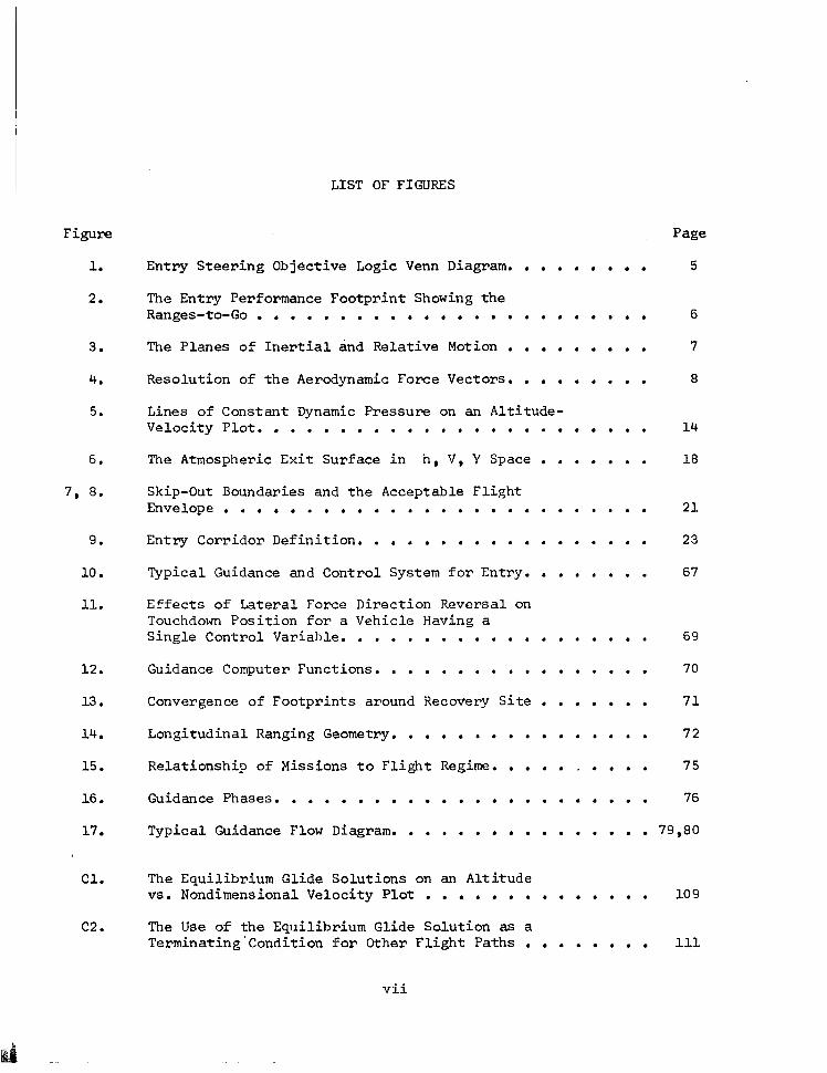
LIST OF FIGURES

Figure

1.

2.

3.

4.

5.

6.

7, 8.

9.

10.

11.

12.

13.

14.

15.

16.

17.

Cl.

c2.

Entry Steering Objective Logic Venn Diagram. . . . . . . . .

The Entry Performance Footprint Showing the Ranges-to-Go . . . . . . . . . . . . . . . . . . . . . . . .

The Planes of Inertial and Relative Motion . . . . . . . . .

Resolution of the Aerodynamic Force Vectors. . . . . . . . .

Lines of Constant Dynamic Pressure on an Altitude- Velocity Plot. . . . . . . . . . . . . . . . . . . . . . . .

The Atmospheric Exit Surface in h, V, Y Space . . . . . . .

Skip-Out Boundaries and the Acceptable Flight Envelope................ . . . . . . . . . .

Entry Corridor Definition. . . . . . . . . . . . . . . . . .

Typical Guidance and Control System for Entry. . . . . . . .

Effects of Lateral Force Direction Reversal on Touchdown Position for a Vehicle Having a Single Control Variable. . . . . . . . . . . . . . . . . . .

Guidance Computer Functions. . . . . . . . . . . . . . . . .

Convergence of Footprints around Recovery Site . . . . . . .

Longitudinal Ranging Geometry. . . . . . . . . . . . . . . .

Relationship of Missions to Flight Regime. . . . . _ . . . .

Guidance Phases. . . . . . . . . . . . . . . . . . . . . . .

Page

5

6

7

8

14

18

21

23

67

69

70

71

72

75

76

Typical Guidance Flow Diagram. . . . . . . . . . . . . . . . 79,80

The Equilibrium Glide Solutions on an Altitude vs. Nondimensional Velocity Plot . . . . . . . . . . . . . . 109

The Use of the Equilibrium Glide Solution as a Terminating'condition for Other Flight Paths . . . . . . . . 111

vii

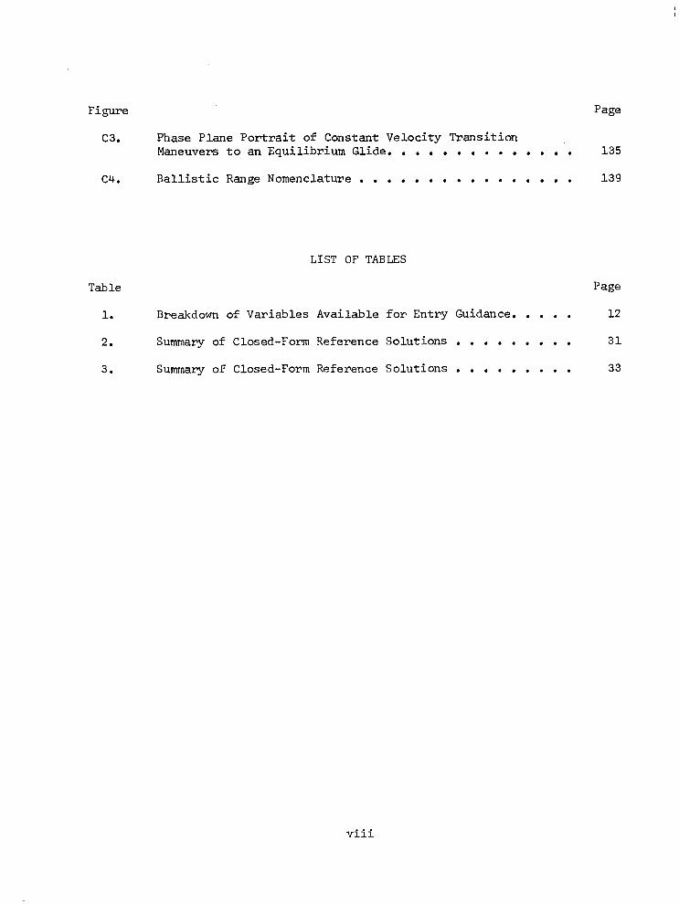
Figure Page

c3. Phase Plane Portrait of Constant Velocity Transition Maneuvers to an Equilibrium Glide. . . . . . . . . . . . . . 135

c4. Ballistic Range Nomenclature . . . . . . . . . . . . . . . . 139

LIST OF TABLES

Table Page

1. Breakdown of Variables Available for Entry Guidance. . . . . 12

2. Summary of Closed-Form Reference Solutions . . . . . . . . . 31

3. Summary of Closed-Form Reference Solutions . . . . . . . . . 33

viii

LIST OF SYMBOLS

Btglish Symbols

CL CD CR CY CH C

D D

smoothed sensed acceleration horizontal acceleration acceleration vector

aerodynamic lift coefficient aerodynamic drag coefficient resultant aerodynamic force coefficient aerodynamic side force coefficient aerodynamic heat transfer coefficient aerodynamic control vector

aerodynamic drag force of log10 (V2/a) aerodynamic drag force vector

p%RO aerodynamic force vector derivative vector function of the state vector or force vector

-F

h H hS H

ii L L

m R M

P

5

: RE

matrix of partial derivatives of time-dependent elements with respect to the state

gravitational acceleration aerodynamic load factor partial derivative of time-dependent elements a F/3:

altitude or angular momentum/unit mass heat energy atmospheric scale height partial of the vector function g with density

aerodynamic lift force vector reference length linear perturbation guidance gain matrix latitude from the equatorial plane

vehicle mass mean molecular weight quadratic gain matrix

pressure or semi-latus rectum distance

dynamic pressure

position vector universal gas constant; or surface arc range Reynolds number

ix

S reference area

T T

absolute gas temperature terminal deviation weighting matrix

U U

horizontal velocity control deviation weighting matrix

V

1

9

VR V

vertical velocity or altitude rate inertial or relative velocity vector relative velocity vector ratio of velocity to circulas orbit velocity at planet surface unit vector in relative velocity direction state vector deviation weighting matrix

x state vector

Y lateral acceleration magnitude

2 Z

Chapman function velocity-dependent linear perturbation guidance control variable

angle of attack inverse of the atmospheric scale height flight path angle orbit energy weighted mean value of CR/CD ballistic range to apoapse downrange-to-go, true anomaly longitude angle from prime meridian linear perturbation guidance matrix solutions atmospheric viscosity; gravitational constant atmospheric density crossrange-to-go bank angle state transition matrix azimuth (heading) angle terminal objective vector planet angular velocity vector terminating condition

C commanded value CIR circular DES desired value

Greek Symbols

Subscripts

E, EQUIL EXIT f G i k LIM MAX MEAS MIX N P P R REF S t TRANS v

T . A

equilibrium glide

exit value final value constant G value initial value or summation arbitrary element in a set of elements limiting value maximum value measured value minimum value nominal trajectory value planet periapse relative to rotating planet reference trajectory value scale or standard terminating value transition value velocity-dependent

Superscripts

transpose time derivative unit vector

xi

1.0 STATEMENT OF THE PROBLEM

The problem of braking a vehicle in the vicinity of a planet having an atmosphere, with the objective of either landing on the planet's surface or to be captured by its gravitational field, has two distinct methods of solution. However, both of these solutions require a force component acting in a direction opposite to the motion to decrease the angular momentum and the energy of the trajectory with respect to the planet. The first (propulsive) solution requires that the force be applied to the expense of the vehicle carrying an available chemical or nuclear supply of energy. The second relies on the gasdynamic drag while passing through the planet's atmosphere and dissipates the vehicle's kinetic energy in the form of heat. (The magnitude of the fraction of this heat energy which can be transferred to the atmosphere in the process is the deciding factor in determining which of the two methods is the more practical solution.)

This Monograph will be directed to the second of these solutions. That is, it is assumed that a sufficiently large fraction of the vehicle's kinetic energy can be transferred to heating the atmosphere to justify the aero-braking solution for a given mission. Therefore, the conditions under which the flow processes can fulfill this transfer must be insured by controlling the vehicle's flight path during entry. However, if the vehicle is manned, its crew must be protected from large accelerations; this requirement further restricts the vehicle's flight path and results in increased level of sophistication in trajectory control. These conditions constitute the fundamental requirements for entry guidance.

The next logical step, in the direction of increased entry guidance sophistication, is to require that the system deliver the vehicle to a desired terminal state. (The terminal state can be a prescribed landing site or a specified conic upon exiting from the atmosphere.) Thus, the atmospheric entry guidance system has a dual role, i.e., to control the vehicle's flight path such that the gasdynamic flow effects do not exceed the limits of the vehicle and its crew, and to satisfy a set of terminal objectives. To fulfill this dual role, a large number of entry guidance schemes have been proposed; of these, a small number have been investigated by means of a detailed computer simulation, and an even smaller number, by actual flight test. Even so, there is an extremely large amount of material available and it is necessary to restrict the scope of the investigation so as to provide the maximum of insight into the problems of greatest interest. For this reason, no consideration is given to the control of steep ballistic entries or orbit decay trajectories. With these special cases omitted, it is safe to say that an open-loop approach to the entry guidance problem, in most cases, is not satisfactory due to uncertainties in the atmospheric and in the aerodynamic force coefficients. Thus, continuous (or discrete) monitoring of the vehicle's state and a corresponding updating of control is necessary.

1

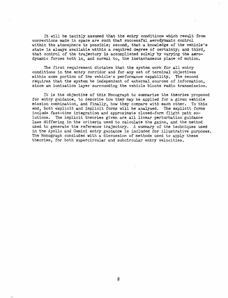
It will be tacitly assumed that the entry conditions which result from corrections made in space are such that successful aerodynamic control within the atmosphere is possible; second, that a knowledge of the vehicle's state is always available within a required degree of certainty; and third, that control of the trajectory is accomplished solely by varying the aerodynamic forces both in, and normal to, the instantaneous plane of motion.

The first requirement dictates that the system work for all entry conditions in the entry corridor and for any set of terminal objectives within some portion of the vehicle's performance capability. The second requires that the system be independent of external sources of information, since an ionization layer surrounding the vehicle blocks radio transmission.

It is the objective of this Monograph to summarize the theories proposed for entry guidance, to describe how they may be applied for a given vehicle mission combination, and finally, how they compare with each other. To this end, both explicit and implicit forms will be analyzed. The explicit forms include fast-time integration and approximate closed-form flight path solutions. The implicit theories given are all linear perturbation guidance laws differing in the criteria used to calculate the gains, and the method used to generate the reference trajectory. A summary of the techniques used in the Apollo and Gemini entry guidance is included for illustrative purposes. The Monograph concludes with a discussion of methods used to apply these theories, for both supercircular and subcircular entry velocities.

I

2.0 STATE-OF-THE-ART

2.1 PHILOSOPHY OF ENTRY GUIDANCE

Numerous methods have been proposed for guiding the flight of an entry vehicle provided with the capability for aerodynamically altering,its trajectory. The basis for these methods include the following techniques:

. on-board calculation of future trajectories using approximate expressions

. storage of trajectories and control gains

. on-board fast-time integration of future trajectories

The majority of the guidance schemes in the literature use one or more of these techniques in a given application. Most of the schemes, however, employ only one of the methods listed. The use of both stored trajectory data and on-board calculated reference solutions enjoys current popularity, and is described in its Apollo application. Certain promising combinations, such as a composite mechanization utilizing closed form approximate expressions with stored control gains, have not yet been investigated. No papers on fast-time integration guidance have been published in the guidance literature in recent years. This lack of emphasis is most likely due to the extreme sensitivity of the integration to variations in aerodynamic control and initial conditions at near-circular and supercircular orbit velocities.

At the time of this writing, entry guidance laws have not been demon- strated to be as amenable to sophistication and optimization as have boost and space guidance. This observation is partly the result of the vehicle/crew limits, (which play an important role in the steering law selection process), and partly the result of unavoidable buildup of relatively large inertial measurements errors. A third probable reason is that the mathematical form and the point mass equations of motion are complex when aerodynamic forces are included. Thus, the current guidance philosophy is not to optimize a steering law in the sense that the closed-loop "footprint" is maximized. Rather, the accuracy and reliability of the system over restricted, operational performance limits is considered to be more important.

This subsection has been prepared to place the steering law selection in its proper perspective with other entry systems design problems. Accordingly, the steering objectives, the steering objective selection logic (when multiple objectives are involved), the navigational and other measurement data available, and the implications of the vehicle/crew limits on the guidance problem will be described. The secondary purpose of this discussion is to introduce the nomenclature and terms used in the theory and applications subsections.

3

2.1.1 Steering Objectives

In general, missions incorporating an atmospheric entry phase have at least one of the following as entry steering objectives: a terminal location on the planet surface, a Keplerian conic trajectory in the upper limits of the atmosphere, or a prescribed flight environment. Whereas the primary trajectory control mechanism (i.e., energy dissipation rate) is not directly related to the steering objective for the first two objectives listed, this mechanism itself may be the objective in the case of the flight environment steering objective. (Such is the case when the objective is a gas dynamic environment-oriented test.) When the vehicle/crew limits are critical, the flight environment objective is to fly within a safe and acceptable flight envelope. This topic is discussed later.

The major portion of the papers on entry guidance are concerned with the terminal ranging objective. This problem is primarily one of controlling the vehicle's energy dissipation rate such that a major fraction of the vehicle's energy is lost at a time when the vehicle arrives over the desired destination. For this application, the guidance system acts as an energy management device.

There is little written in the guidance literature on the general conic trajectory steering objective for entry. To date, only the range performance aspect of conic trajectory guidance has been considered important. Thus, the terminal ranging objective will receive the major portion of the attention in this Monograph. The theories and techniques discussed here, however, can be applied for most applications regardless of the objective, if slight modifications are permitted.

In cases where the mission has more than one steering objective and the possibility exists of not satisfying all of them simultaneously, it becomes necessary to assign some preference among the objectives. The logic used in selecting the objective is dependent on which of the steering objectives is considered most critical at the time. For example, when it is not possible to satisfy both the terminal ranging and a restricted flight environment objective simultaneously, the flight environment objective is usually considered to be more critical and therefore is chosen to be the governing objective. This logic can also be expressed in mathematical form. For instance, in the example just mentioned, let A denote the set of all possible future trajectories starting at an arbitrary point along the entry path, and let the symbols M, E, denote the subsets of A satisfying the terminal ranging and the flight environment objectives, respectively. The steering objective selection logic considers two possibilities: The two subsets intersect (M n E # ii+, or they do not intersect (M n E = $). When the subsets intersect each other, both objectives can be satisfied simultaneously and the steering control is selected from the intersecting trajectories. When the subsets do not intersect, only one of the objectives can be satisfied. In this case, the steering is based on controlling for the flight environment objective alone. This logic is illustrated in the form of a Venn diagram in Figure 1. ------------------------------------- @ denotes the empty set

4

-... ---------x All Future Trajectories -‘---A\

Control is Selected From the Intersection of the Two Subsets

Control is Selected From the Flight Envelope Subset

Figure 1 Entry Steering Objective Logic Venn Diagram

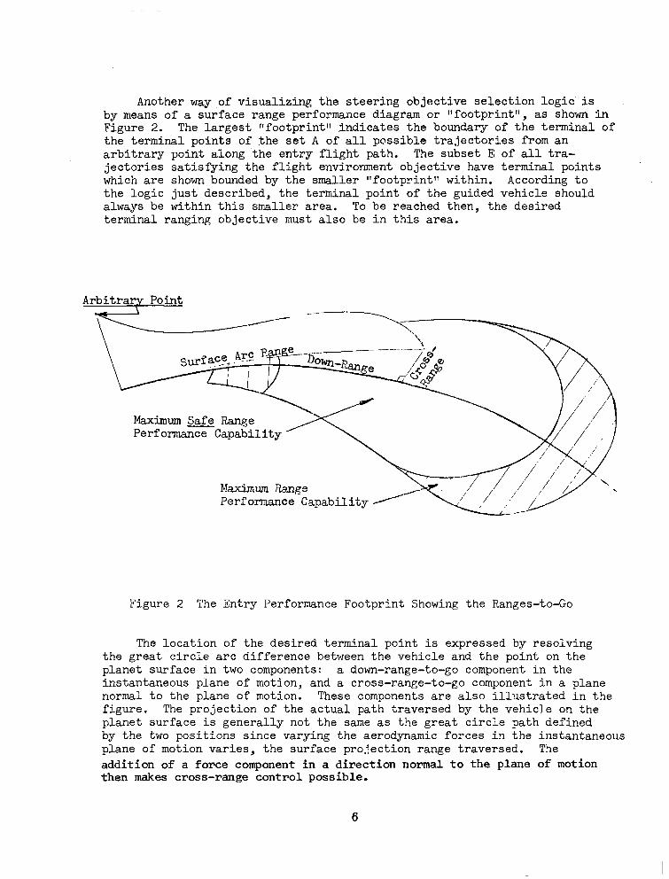
Another way of visualizing the steering objective selection logic is by means of a surface range performance diagram or l'footprint", as shown in Figure 2. The largest "footprint" indicates the boundary of the terminal of the terminal points of the set A of all possible trajectories from an arbitrary point along the entry flight path. The subset E of all trajectories satisfying the flight environment objective have terminal points which are shown bounded by the smaller "footprintI within. According to the logic just described, the terminal point of the guided vehicle should always be within this smaller area. To be reached then, the desired terminal ranging objective must also be in this area.

Arbitrary Point

Maximum-Range Performance Capability

Maximum Range Performance Capability

Figure 2 The Entry Performance Footprint Showing the Ranges-to-Co

The location of the desired terminal point is expressed by resolving the great circle arc difference between the vehicle and the point on the planet surface in two components: a down-range-to-go component in the instantaneous plane of motion, and a cross-range-to-go component in a plane normal to the plane of motion. These components are also illustrated in the figure. The projection of the actual path traversed by the vehicle on the planet surface is generally not the same as the great circle path defined by the two positions since varying the aerodynamic forces in the instantaneous plane of motion varies, the surface projection range traversed. The addition of a force component in a direction normal to the plane of motion then makes cross-range control possible.

6

2.1.2 TheAeyodyn~~_cControl~Vector and tklehicle- Point Mass Equations of Motion

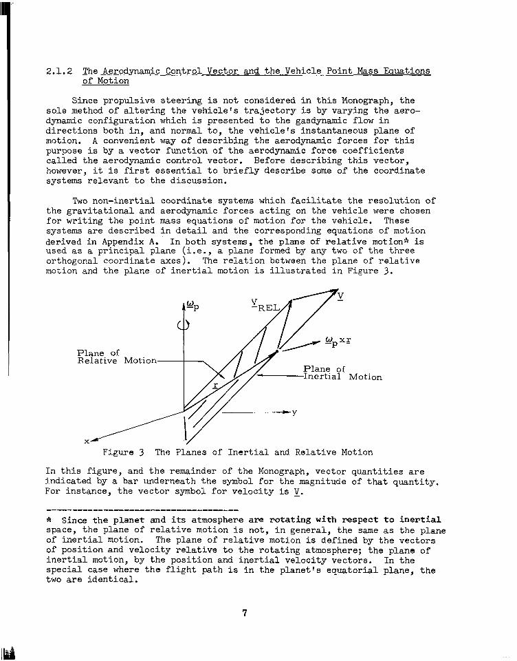
Since propulsive steering is not considered in this Monograph, the sole method of altering the vehicle's trajectory is by varying the aerodynamic configuration which is presented to the gasdynamic flow in directions both in, and normal to, the vehicle's instantaneous plane of motion. A convenient way of describing the aerodynamic forces for this purpose is by a vector function of the aerodynamic force coefficients called the aerodynamic control vector. Before describing this vector, however, it is first essential to briefly describe some of the coordinate systems relevant to the discussion.

Two non-inertial coordinate systems which facilitate the resolution of the gravitational and aerodynamic forces acting on the vehicle were chosen for writing the point mass equations of motion for the vehicle. These systems are described in detail and the corresponding equations of motion derived in Appendix A. In both systems, the plane of relative motionss is used as a principal plane (i.e., a plane formed by any two of the three orthogonal coordinate axes). The relation between the plane of relative motion and the plane of inertial motion is illustrated in Figure 3.

Plane of Relative Motion

Plane of Inertial Motion

Figure 3 The Planes of Inertial and Relative Motion

In this figure, and the remainder of the Monograph, vector quantities are indicated by a bar underneath the symbol for the magnitude of that quantity. For instance, the vector symbol for velocity is 1.

* Since the planet and its atmosphere are rotating with respect to inertial space, the plane of relative motion is not, in general, the same as the plane of inertial motion. The plane of relative motion is defined by the vectors of position and velocity relative to the rotating atmosphere; the plane of inertial motion, by the position and inertial velocity vectors. In the special case where the flight path is in the planet's equatorial plane, the two are identical.

7

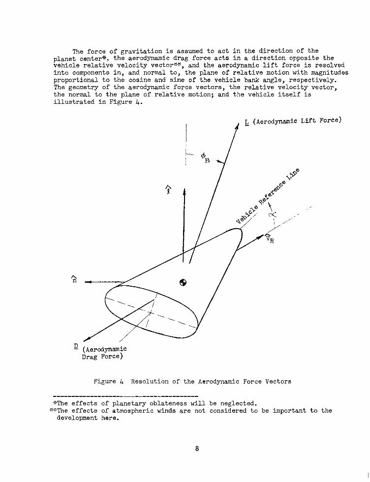
The force of gravitation is assumed to act in the direction of the planet center4kz the aerodynamic drag force acts in a direction opposite the vehicle relative velocity vector%-%, and the aerodynamic lift force is resolved into components in, and normal to, the plane of relative motion with magnitudes proportional to the cosine and sine of the vehicle bank angle, respectively. The geometry of the aerodynamic force vectors, the relative velocity vector, the normal to the plane of relative motion; and the vehicle itself is illustrated in Figure 4.

4 (Aerodynamic Lift Force)

Figure 4 Resolution of.the Aerodynamic Force Vectors

-------------------_------------------- *The effects of planetary oblateness will be neglected.

+j+The effects of atmospheric winds are not considered to be important to the development here.

8

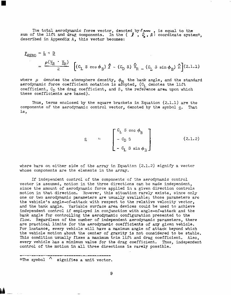
The total aerodynamic force vector, denoted byParr , is equal to the sum of the lift and drag components. In the ( 1" , t, i; ) coordinate system+, described in Appendix A, this vector becomes:

PCLR - 5) =

2 [ (CL S C0S4B) f - (CD S) GR _ (CL 3 sin$B) ~](2.1-1)

where p denotes the atmosphere density, $I 3

the bank angle, and the standard aerodynamic force coefficient notation is a opted, (CL denotes the lift coefficient, CD the drag coefficient, and S, the reference area upon which these coefficients are based).

Thus, terms enclosed by the square brackets in Equation (2.1.1) are the components of the aerodynamic control vector, denoted by the symbol c. That is,

C = -

CL s cos +B

- CD s

- CL S sin +3

(2.1.2)

where bars on either side of the array in Equation (2.1.2) signify a vector whose components are the elements in the array.

If independent control of the components of the aerodynamic control vector is assumed, motion in the three directions can be made independent, since the amount of aerodynamic force applied in a given direction controls motion in that direction. However, this situation rarely exists, since only one or two aerodynamic parameters are usually available; those parameters are the vehicle's angle-of-attack with respect to the relative velocity vector, and the bank angle. Variable surface area devices could be used to achieve independent control if employed in conjunction with angle-of-attack and the bank angle for controlling the aerodynamic configuration presented to the flow. Regardless of the number of independent aerodynamic parameters, there are practical limits for the aerodynamic coefficients of any given vehicle. For instance, every vehicle will have a maximum angle of attack beyond which the vehicle motion about the center of gravity is not considered to be stable. This condition usually fixes a maximum trim lift and drag coefficient. Also, every vehicle has a minimum value for the drag coefficient. Thus, independent control of the motion in all three directions is rarely possible.

------------------------------------- g&The symbol A signifies a unit vector.

9

The equations which relate the aerodynamic and gravitational forces acting on the vehicle to the acceleration of a mass particle which is equal to the total vehicle mass and which is located at the vehicle's center of gravity are the point mass equations of motion. Since these equations are fundamental to all studies concerned with entry performance and guidance, they are the next topic of concern. The control equations and solutions describing the vehicle's rigid body motion about the center of gravity will not be considered though it is noted that motions may be important to the operation of the guidance system if their characteristic frequencies are near the natural frequency of the guidance loop. For this discussion, however, the rigid body control equations are assumed to provide ideal response characteristics (i.e., instantaneous, and no overshoot). Non-ideal response characteristics in the control system can be considered along with uncertainties in the atmosphere and in the aerodynamic force coefficients as contributing factors to open-loop trajectory dispersion. These factors then serve to reinforce the need for a closed-loop approach.

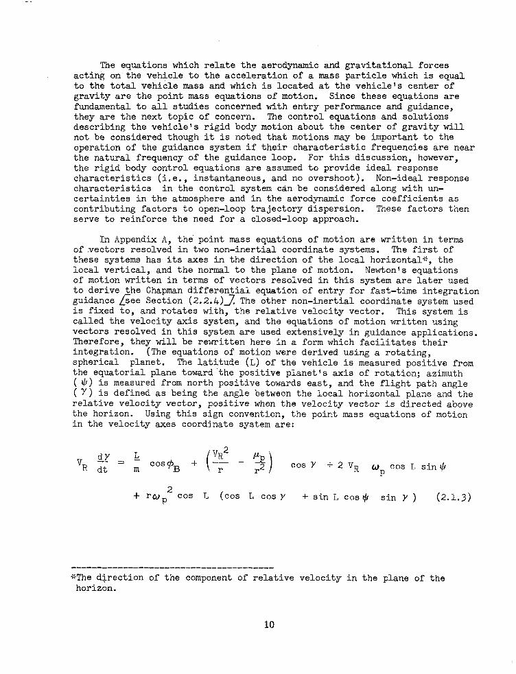
In Appendix A, the. point mass equations of motion are written in terms of vectors resolved in two non-inertial coordinate systems. The first of these systems has its axes in the direction of the local horizontal+, the local vertical, and the normal to the plane of motion. Newton's equations of motion written in terms of vectors resolved in this system are later used to derive the Chapman differential equation of entry for fast-time integration guidance Lsee Section (2.2.4)_;;! Th e other non-inertial coordinate system used is fixed to, and rotates with, the relative velocity vector. This system is called the velocity axis system, and the equations of motion written using vectors resolved in this system are used extensively in guidance applications. Therefore, they will be rewritten here in a form which facilitates their integration. (The equations of motion were derived using a rotating, spherical planet. The latitude (L) of the vehicle is measured positive from the equatorial plane toward'the positive planet's axis of rotation; azimuth ( $!J) is measured from north positive towards east, and the flight path angle ( Y) is defined as being the angle between the local horizontal plane and the relative velocity vector, positive when the velocity vector is directed above the horizon. Using this sign convention, the point mass equations of motion in the velocity axes coordinate system are:

V dr = L vR2 PJ R dt

m COS(pB + -F - r2 cos Y + 2 vq

* OP cos 1, sin $

+ rcdD2 cos L (cos L cos y + sin 'I, cos $ sin Y ) (2.1.3) L

------_-------------------------------- *The direction of the component of relative velocity in the plane of the

horizon.

10

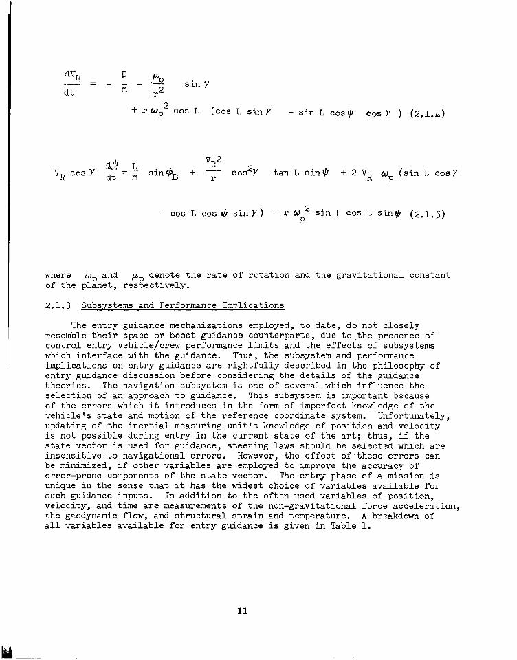
dV, * P

dt = a

m - -0 r2

siny

+ rWp2 cc-s T, (cos I, sinY - sin L COSJ, cos Y ) (2.1.4)

cos2Y tan I. sin+ + 2 VR o, (sin L cos Y

- cos L cos !Ir sinY) -I- r tin2 sin T, cos T.. sing (2.1.5)

where &P and pp denote the rate of rotation and the gravitational constant of the planet, respectively.

2.1.3 Subsystems and Performance Implications

The entry guidance mechanizations employed, to date, do not closely resemble their space or boost guidance counterparts, due to.the presence of control entry vehicle/crew performance limits and the effects of subsystems which interface with the guidance. Thus, the subsystem and performance implications on entry guidance are rightfully described in the philosophy of entry guidance discussion before considering the details of the guidance theories. The navigation subsystem is one of several which influence the selection of an approach to guidance. This subsystem is important because of the errors which it introduces in the form of imperfect knowledge of the vehicle's state and motion of the reference coordinate system. Unfortunately, updating of the inertial measuring unit's knowledge of position and velocity is not possible during entry in the current state of the art; thus, if the state vector is used for guidance, steering laws should be selected which are insensitive to navigational errors. However, the effect of these errors can be minimized, if other variables are employed to improve the accuracy of error-prone components of the state vector. The entry phase of a mission is unique in the sense that it has the widest choice of variables available for such guidance inputs. in addition to the often used variables of position, velocity, and time are measurements of the non-gravitational force acceleration, the gasdynamic flow, and structural strain and temperature. A breakdown of all variables available for entry guidance is given in Table 1.

11

Table 1. Breakdown of Variables Available for Entry Guidance

Differentiated Variables

Non-gravitational force acceleration rate, d&ER&d/dt

Time rate of change of gasdynamic flow measurements

Structural strain and temperature rate

Measured Variables

Non-gravitational force acceleration ' 'AER d m

Gasdynamic flow measurements

Structural strain and temperature

Time, t

Integrated Variables

State vector, & (position and velocity vectors)

Linear perturbation guidance schemes employing state vector components together with the non-gravitational force acceleration and acceleration rate for reference trajectory control are common in the entry guidance literature. Reference 14 contains a development where the use of vehicle skin temperature rate is also suggested for entry guidance.

Another subsystem influencing the selection of the steering law is the guidance computer itself. Such factors as storage space and timing requirements should be examined. However, this aspect of the analysis is considered to be beyond the scope of the current effort.

The vehicle/crew performance limits having guidance implications can be classified into two types: time-dependent and non-time-dependent. Time dependent limits, in general, may be expressed in integral form; the integration performed using time as the independent variable with initial and final flight times as limits. Some examples of this type of limit include the fraction of the total energy (heat) input to the vehicle, and entry time. Non-time dependent limits may be thought of as point constraints. Some examples of this type include maximum aerodynamic load factor (acceleration level), and maximum heat transfer rate. The existence of both the time- and non-time-dependent limits for a given vehicle/crew combination imply that, in the process of steering for terminal objectives, the vehicle must be in a safe acceptable flight envelope whose boundaries are determined by the aforementioned limits. As expected, most of the entry performance limits arise from gasdynamic flow effects on the vehicle. A discussion of these effects, the nature of the limits, and their transformation into flight boundaries follows.

12

I --

2.1.3.1 Gasdynamic Flow Effects

Primary among the gasdynamic flow effects are the vehicle's aerodynamic acceleration and heating. The aerodynamic acceleration is proportional to the resultant aerodynamic force for a fixed mass vehicle and may be separated into two factors; the first is the dynamic pressure (a function of the vehicle's altitude and velocity). The second is the aerodynamic control vector, whose components are varied for steerage. The proportionality of the non-gravitational acceleration on dynamic pressure makes it convenient to portray lines of constant acceleration on an altitude-velocity plot for a fixed angle-of-attack vehicle in terms of lines of cons&ant dynamic pressure. Now, since the dynamic pressure, denoted by the symbol q (the overhead bar does not signify a vector) is given by the expression,

p !2F * v,! ;;= --. 2 = 2 p 52 (2.1.6)

then by substituting the exponential atmosphere model, Equation (B-2a), another expression relating altitude to velocity for constant dynamic pressure can be obtained, i.e.,

= 2hs In

(2.1.7)

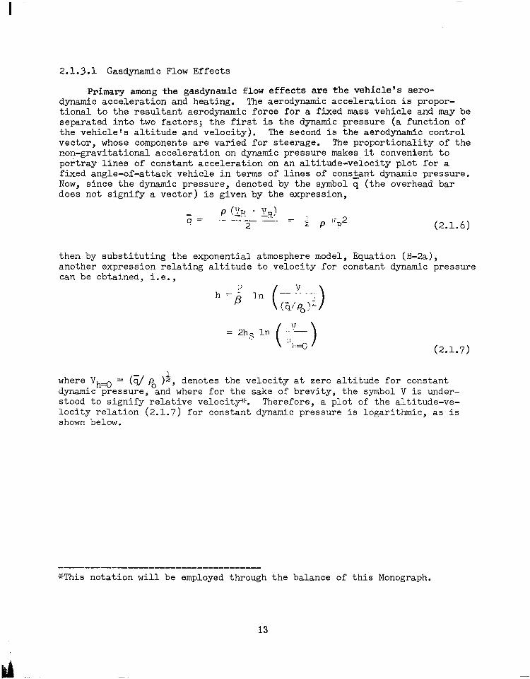
where Vh4 = (-4 p, )h, denotes the velocity at zero altitude for constant dynamic pressure, and where for the sake of brevity, the symbol V is under- stood to signify relative velocity+. Therefore, a plot of the altitude-velocity relation (2.1.7) for constant dynamic pressure is logarithmic, as is shown below.

----m-w-- ---------------m-

+This notation will be employed through the balance of this Monograph.

13

d

h

direction of decreasing dynamic pressure

dynamic pressure

Vh= 0 V-

Figure 5 Lines of Constant Dynamic Pressure on an Altitude-Velocity Plot

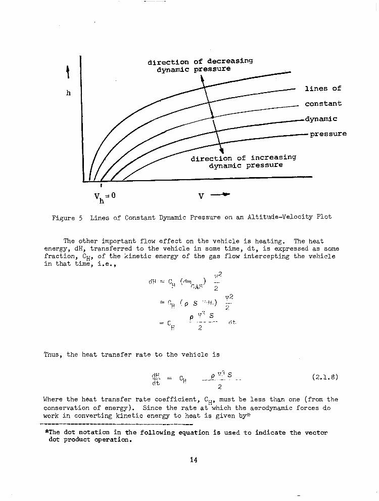
The other important flow effect on the vehicle is heating. The heat energy, dH, transferred to the vehicle in some time, dt, is expressed as some fraction, CH, of the kinetic energy of the gas flow intercepting the vehicle in that time, i.e.,

Thus, the heat transfer rate to the vehicle is

--._..-. P r ? ,,_ (2.1.8)

Where the heat transfer rate coefficient, CH, must be less than one (from the conservation of energy). Since the rate at which the aerodynamic forces do work in converting kinetic energy to heat is given by+

---------------------------------------- *The dot notation in the following equation is used to indicate the vector

dot product operation.

14

I

V

EA,YO * 71 -I?

= 9 * ID = c, 2 _ .9 .__ . (2.1.9) . 2

and, since this conversion results in heating the atmosphere and the vehicle, the ratio CH/CD also must be less than one. This ratio represents the portion of the work which goes into heating the vehicle. In Reference 4 the heat transfer coefficient is broken down into three components: a convective component strongly dependent on the nature of the boundary layer, a radiative component due to radiation of the hot gas in chemical equilibrium, and a nonequilibrium radiative component. It suffices to say that the heat transfer coefficient is not a simple function, and must take into account the effects of body geometry, density, atmospheric constitutes, velocity, and the nature of the boundary layer.

The total++ heat input to the vehicle on a trajectory is the time integral of the heat transfer rate dH/dt, thus

t f

I-! =

/

c P IT3 s

d.t H - 2.--

(2.1.10)

where the subscripts ltiif and Irflf indicate the initial and final atmospheric flight times. This integral can be transformed into a velocity dependent integral for small flight path angle trajectories by the differential transformation:

dt dV -- dt = iiF dlJ = -

(D/m!

(2.1.11)

Substituting (2.1.11) for the differential time into (2.1.10) and changing the limits of integration then yields

(2.1.12)

---_______----------_______________I_

*The resultant heat input is always less since it accounts for the reradiative heat transfer from the vehicle to the surrounding atmosphere.

15

Thus, for constant mass, the total heat input can be expressed as a fraction of the initial kinetic energy, i.e.,

m V 2

F! = i 37------ (2.1.13)

2

where q is a weighted mean value of (CH/CD> given by

1.

(2.1.14)

IT /T7 fi

2.1.3.2 Vehicle/Crew Limits

Several of the vehicle and crew limits have important implications for entry guidance; some of these factors are: the vehicle structural load limit, the aerodynamic heat transfer rate limit, the maximum total heat input to the vehicle, maximum entry time, and the crew's tolerance to acceleration. However, not all of these limits are used to define the safe flight regime. For instance, in most manned vehicles, the crew's tolerance to acceleration (aerodynamic load factor) is a more limiting factor than the structural load factor; thus, a guidance law satisfying the former would always restrict the trajectory to satisfy the latter. The aerodynamic load factor is defined in terms of the ratio of the resultant aerodynamic force to the weight of the vehicie, i.e.,

I c 4 W’ I f-,S

-- r7 = ----- .-- =

‘.li hl ‘i (2.1.15)

where CR denotes the resultant aerodynamic force coefficient given by

cR = (CL2 + CD2 + Cy2)f

23 or, for a vehicle trimmed to zero yaw angle, CY = 0, and CR = (CL2 + CL, )

Assuming the resultant aerodynamic coefficient is constant, the proportionality of the aerodynamic load factor to dynamic pressure makes it convenient to portray lines of constant load factor as shown in Figure 5. This is often the assumption used for fixed angle-of-attack vehicles.

Since the heat-protection systems for most entry vehicles are either ablative or reradiative in their method of operation, the entry vehicle will most likely be limited to either a maximum total heat input Hmax or a limiting value of heat transfer rate dH/dt-. This limitation arises since the mass loss due to abiation is roughly proportional to the total heat input

16

due to the fact that the reradiative structure, whose operation depends on the radiating of heat away from the skin, is temperature-limited.

The remaining limit to be considered is that of the crew. The systems implications of this limit, in the case of earth entry, are many; however. only the guidance aspect will be considered. Reference 5 contains data indicating that pilot's tolerance to acceleration may be expressed as a maximum value for the product Gmt where m is an exponent whose value is dependent on the pilot's orientation relative to the imposed acceleration, and t is the time spent at the given value of G. A more general empirical approach can be used to formulate crew limits in terms of a maximum value for the integral

t I7 t-

i.

This criteria is called the acceleration dosage. However, since neither of these two approaches is amenable for guidance purposes, a limiting value of the nondimensional aerodynamic acceleration is often used to indicate the pilot and crew limits.

2.1.3.3 Atmospheric Exit Boundaries

One factor in determining the flight envelope available for trajectory control is the consequence of the vehicle inadvertantly exiting;: from the atmosphere. The controlled exit maneuver, on the other hand, is a useful maneuver to extend the range performance of the vehicle after the initial entry. However, atmospheric exits can result in prolonged flights which may exceed certain system limits and which can result in large range errors. Thus, to prevent unwanted supercircular atmospheric exits, those sets of flight conditions,' (namely altitude, velocity, and flight path angle) which aiways result in an exit condition for a given vehicle, must be determined. This objective can be accomplished by integrating (numerically or otherwise) a family of trajectories for a series of initial altitudes, velocities, and flight path angles, employing the vehicle's full negative lift capability. In this manner, the region of (h, V, Y) space where the vehicle exits, regardless of the degree of control exerted, may be found for any given configuration. The boundary of this region in (h, V, Y) space defines an atmospheric exit surface for that vehicle which can be expressed in the following mathematical form:

(2.1.16) ----------------_-__________^_________

*Atmospheric exit is defined to occur when the vehicle reaches a minimum defined value of aerodynamic acceleration with a positive altitude rate. Other defini- tions (e.g., based on altitude) of the exit condition are also used for convenience. In any study any such reasonable definition may be adopted, provided the definition is consistent in actual usage.

17

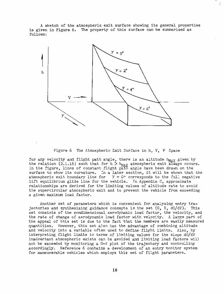
A sketch of the atmospheric exit surface showing its general properties is given-in Figure 6. The property of this surface can be summarized as follows:

Figure 6 The Atmospheric Exit Surface in h, V, Y Space

for any velocity and flight path angle, there is an altitude h the relation (2.1.16) such that for h > h

X given by

Y atmospheric exit a ways 9 occurs.

In the figure, lines of constant flight pat angle have been drawn on the surface to show its curvature. In a later section, it will be shown that the atmospheric exit boundary line for Y = O" corresponds to the full negative lift equilibrium glide line for the vehicle. In Appendix C, approximate relationships are derived for the limiting values of altitude rate to avoid the supercircular atmospheric exit and to prevent the vehicle from exceeding a given maximum load factor.

Another set of parameters which is conveni.ent for analyzing entry trajectories and synthesizing guidance concepts is the set (G, V, dG/dV). This set consists of the nondimensional aerodynamic load factor, the velocity, and the rate of change of aerodynamic load factor with velocity. A large part of the appeal of this set is due to the fact that the members are easily measured quantities. However, this set also has the advantage of combining altitude and velocity into a variable often used to define flight limits. Also;by interpreting flight limits in terms of limiting values for the slope dG/dV inadvertant atmospheric exists can be avoided and limiting load factors will not be exceeded by monitoring a G-V plot of the trajectory and controlling accordingly. Reference 6 contains a development of an entry monitor system for maneuverable vehicles which employs this set of flight parameters.

18

The equivalence of the two sets (h, V, Y) and (G, V, dG/dV) can be shown for vehicles having constant aerodynamic force coefficients. The aerodynamic load factor is related to altitude and velocity for a given atmospheric model (B-2) by the expression

G = r, (h, 11 rl s p. exp (-Ph) V2

)= -;- (2.1.17) 2

Thus, the total differential of G is given by

The total rate of change in G with velocity for constant aerodynamic force coefficients is now obtained as:

dG = g dh aG = ah dVfTE

CR s V2 dh dt CR S z 7 (-F) PO exp (-Bh) 2 dt G-P 7 p. exp (-oh) v

CR ', V2 =-

V sinY CR S

w (--PI po eq (-$h) 2

- D/m -pO eXP (-oh) v (2.1.18) W

'R ' B m - PO exp (-Oh) -V sinY -i- V

w 'D s

where the small flight path angle and nonrotating atmosphere Lpproximations were used in substituting for the term (dt/dV). Therefore, the slope of the aerodynamic load factor versus velocity plot has one component proportional to V sin Y ( or h, the altitude rate) and the other proportional to velocity, as shown in (2.1.18). Equation (2.1.18) correlates the three variables (h, V, Y) with (dG/dV) in the sense that, given any three, the remaining variable is determined from (2.1.18). Therefore, the equivalence of the sets (h, V, I') and (G, V, dG/dV) has been shown. The atmos'pheric exit surface illustrated in Figure 6 may then be transformed into a surface in (G, V, dG/dV) space', if desired.

19

2.1.3.4 Tie Safe Acceptable Flight Envelope

In the last few pages, the vehicle/crew limits and the concept of a limiting flight condition surface in j-space have been introduced. It now remains to transform these limits into the surface of an acceptable flight envelope within which the entry vehicle must fly. The non-time-dependent limits can be transformed directly; the time-dependent limits are transformed by introducing an intermediate variable more directly related to the set of flight conditions. For the non-time-dependent limits, such as aerodynamic load factor and heating rate, limiting surfaces in altitude-velocity-flight path angle space are obtained by backwards integration of trajectories from a flight limit tangency condition using the maximum vertical lift capability. In the case of time-dependent limits, such as maximum entry time and heat input, these limits can very often be related in an approximate sense with entry range or a non-exit condition.

In any case, it is sufficient to say that the surface (a function of all flight parameters) incorporating all vehicle/crew limits constitutes what will be referred to as the flight envelope. This envelope may be shown in the (h, V, Y) or (G, V, dG/dV) three-dimensional spaces, or in two-dimensional form as illustrated in Figures 7 and 8. In these figures the atmospheric exit surfaces (indicated by lines of constant flight path angle in the h - V plane, and lines of the slope dG/dV in the GV plane) are used to define a portion of the flight envelope. Other flight limits shown are in two-dimensional form and include lines of limiting aerodynamic heat transfer rate and acceleration. The effect of the time-integrated vehicle and crew limits, such as the total heat input limit can be better shown, however, on a plot of the vehicle range capability if so desired. Thus, the implications of the vehicle/crew limits on guidance are: to guide the vehicle into the acceptable flight envelope and to maintain the vehicle's position within the envelope.

20

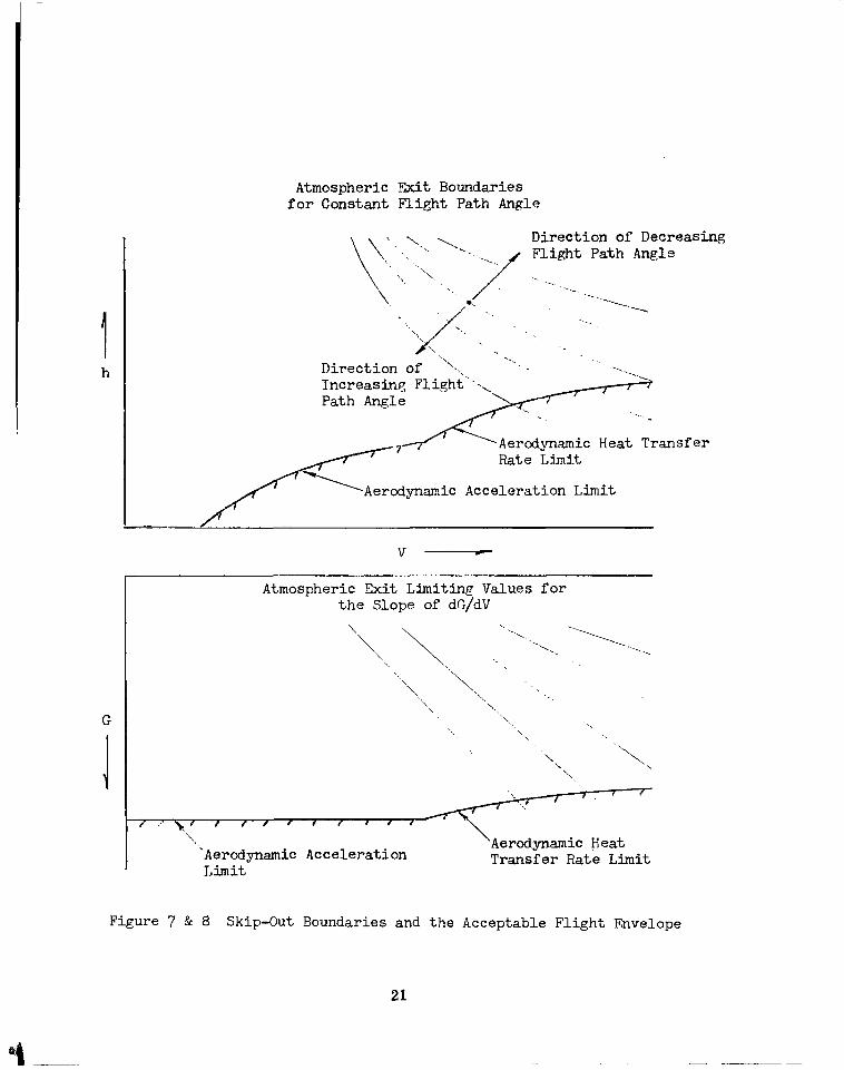
Atmospheric Flit Boundaries for Constant Flight Path Angle

Direction of Decreasing Flight Path Angle

Direction of

~LL~e -2 Atmospheric Exit Lxnltmg Values for

Figure 7 & 8 Skip-Out Boundaries and the Acceptable Flight Envelope

21

2.1.3.5 Entry Corridors

In the preceding section, the geometry of the vehicle's acceptable flight envelope was discussed. It was shown that these limiting flight surfaces result since only a limited amount of trajectory control is available to the vehicle. These surfaces, when extended to the upper limits of the atmosphere, enclose a region in which the vehicle must fly during the initial penetration of the atmosphere (For earth entry, the initial penetration is defined to occur when the vehicle passes through the .!+OO,OOO foot altitude level with a negative altitude rate.)+

For most applications, the initial entry velocity vector is determined to a great extent by mission considerations. However, for most missions, the entry velocity in magnitude is nearly fixed. Thus, the initial flight path angle must be limited in order that the vehicle can safely maneuver into the acceptable flight envelope. The variation in the acceptable initial flight path angle depends mainly on the amount of lift made available for the initial entry maneuver; the largest entry flight path angle is determined by a maximum-vertical-lift trajectory which is tangent to the lower altitude boundary of the flight envelope. This condition is referred to as the "undershoot" boundary. The shallowest entry flight path angle is usually determined by the atmospheric capture requirement. This condition determines the I'overshoot" boundary. For initial flight path angles shallower than this value, atmospheric exit results. The overshoot flight path angle is identical to the angle associated with the atmospheric exit boundary line in the h-V plane which passes through the point determined by the initial entry altitude and velocity.

By extending the trajectories associated with the undershoot and overshoot flight path angles as tonics in the assumed absence of an atmosphere, the difference in the implied periapse distances can be determined. This extension is illustrated in Figure 9 for the case where the two radii are aligned in a common direction. The corridor between the undershoot and overshoot tonics (shown in the figure), is referred to as the entry corridor. Besides aerodynami.c lift, the other factors which influence (for the worse) the size of the entry corridor include the vehicle's limited control response time and atmospheric deviations.

+tThis interface altitude is convenient for specifying entry flight path angle limits although operationally the entry phase is normally considered to start upon reaching a certain load factor.

22

vacuum perigee corridor depth,

I- At

vacuum

planet center

sensible atmosphere

Figure 9 Entry Corridor Definition

2.2 GUIDANCE THEORIES

2.2.1 Summary

In the preceding section, the implications of the entry vehicle/crew performance limits were shown to generally result in a dual objective for the guidance system: i.e., to restrict the flight within an acceptable flight envelope, and in the process, to guide the vehicle to a desired destination. The techniques proposed in the literature to satisfy these objectives are basically of three types: linear perturbation guidance employing on-board calculated reference trajectories, linear oerturbation guidance employing stored reference tra.jectories and optiml gains, and fast-time integration guidance+.

Linear perturbation guidance is a method whereby the steering command is formed by a summtion of terms linearly proportional to the deviations (perturbations) of the actual trajectory from a reference trajectory. In the first perturbation guidance technique mentioned, the reference trajectory is calculated on-board the vehicle during entry. In the second, the reference solution is precalculated, (usually on the ground), and the results stored in a memory device for use during entry. An example of a linear perturbation entry guidance law suggested for guidance in the plane of motion is taken from Reference 12, i.e.,

-- L- l$ D ( )

R5F +tl A'h+~2 AA+K~ AR

where the differences in altitude rate, AL , horizontal acceleration, AA , and surface-arc range AR , are evaluated at the same velocity value for the actual and reference trajectories. The proportionality factors, in this case, given by Kl, K2, K3, are called the guidance pains.

--_-_----------------------m---w-a- +Linear perturbation guidance employing stored reference trajectories and

optimal gains is an implicit steering technique. That is, a steering law which generates a command on the basis of deviations in the vehicle's state from a calculated solution. Both the flight envelope and the terminal steering objectives can be satisfied simultaneously with implicit steering if the proper reference solution and gain selection criteria is used. Explicit steering, on the other hand, is a process whereby the steering command is calculated on the basis of a prediction of the vehicle's future path. This technique is used in fast-time integration guidance; linear perturbation guidance employing on-board calculated reference trajectory in effect constitutes a prediction of a future path.

24

The simplest form of linear perturbation guidance law employs gains which do not vary during the time the law is in effect. Constant gain perturbation guidance may be used when the on-board calculated reference trajectory ‘technique is employed. By restricting the gains to constant values, however, the full capability of the linear perturbation guidance method cannot be realized. This fact should be apparent since the constant gain restriction neglects the changing dynamics of the problem; since the sensitivity of the trajectory to perturbations is strongly dependent on where (what time or velocity) the deviations are introduced. Thus a perturbation guidance law which permits variable gains can account for these changing sensitivities during entry.

The second linear perturbation guidance technique is more amenable to variable gains since a large number of calculations is often required to calculate proper (or optimum) gain functions. However, the validity of the optimum gain functions is predicated on the assumption that the resultant tra,jectory lies in the n.eighborhood of the reference solution. This assumption arises because the derivation of the gain functions employs a Taylor series expansion of the equations of motion which is truncated after the linear terms. With the aid of this linear error propagation model, entry guidance gain functions will be derived which satisfy one of two criteria: first, to null deviations in terminal ob,jective with minimum control exerted, and second, to minimize deviations in a function of the terminal objective, errors along the path,and the control exerted. Indeed, these criteria are different and neither includes the other as a special case.

Regardless of when the reference solution is calculated, it is always selected to satisfy a desired performance characteristic. In the case of precalculated solutions, the reference trajectory is usually optimized in the sense of least heat input, least sensitivity to errors, etc. For the on-board calculated approach, the reference trajectory often consists of a closed-form patched solution with the segment end conditions adjusted so as to satisfy an overall entry range requirement. Unless a large number of trajectories are stored, the latter technique is the only reliable entry guidance technique developed which enables a wide range of terminal objectives to be attained. Although the fast-time integration guidance method offers flexibility in terminal objectives, the extreme trajectory sensitivities at orbital and super-orbital velocities makes the reliability of this method questionable when employed with faulty input data. Therefore , perturbation guidance employing on-board calculated reference trajectories appears to be the most promising of the entry guidance techniques developed to date. Its theory follows*

2.2.2 Linearized Perturbation Guidance Employing On-Board Calculated Reference Trajectories

In the summary, the on-board calculated reference trajectory technique was introduced as the most promising entry guidance technique since it has the ability to adapt to a wide range of terminal objectives. However, since no attempt to date has been made to calculate a corresponding set of optimum linearized guidance gain functions on-board (to the knowledge of the authors), this development will emphasize the calculation of the reference trajectory.

25

t %

--

Thus, no attempt will be made to derive a constant-gain selection criteria. Instead, it is believed that this problem lends itself more to an empirical solution. Other alternatives, such as the use of optimum linearized guidance gains for the patched calculated reference trajectory, so as to permit rapid calculation of optimum linearized gain functions, remain to be investigated.

Although it is not possible to integrate the point mass equations of motion for atmospheric flight in an exact closed form, approximate solutions which are sufficiently accurate for reference trajectory guidance applications may be developed if the vehicle is assumed to be controlled to follow certain flight paths. However, even these restricted solutions are, in most cases, limited to an integration of the dynamics in the plane of motion. The exceptions to this are the minor circle turn solution described in Reference 7 and the lateral motion solutions of Reference 8. The integration of the equations of motion for various restricted flight modes is given in Appendix C; however, the assumptions which make the analytic integration possible and approximate are relevant to the discussion of entry guidance and will be listed here. They are:

. The planet and its atmosphere are non-rotating and spherical in shape

. The flight path angle is restricted to small values (usually less than loo) so that its cosine is approximately one and the component of the gravitational attraction along the velocity vector is small in comparison to the aerodynamic drag force

. The exponential atmospheric model is valid

. The height of the atmosphere is small in comparison to the planet radius so that the vehicle's distance from the planet center is approximately the same as the planet's radius during atmospheric flight

These assumptions are definitely restrictive. Thus, the flight path solutions integrated in Appendix C are not valid for steep ballistic entries or entries into deep, rapidly rotating atmospheres, such as encountered about the planet Jupiter. The effect of planet rotation and a non-spherical shape can be compensated for in the guidance logic, by estimating the total flight time and the average component velocities. This modification is discussed in Reference 9 for an application using the equilibrium glide closed form solution. The validity of the atmospheric model has already been discussed in Appendix B. The validity of all the assumptions should be re-examined for any given application of the theory to a specific vehicle and mission, however.

With these assumptions employed, the point mass equations of motion in the velocity axis system are reduced to the following simplified set:

dV = -ii dt m

(2.2.1)

26

I -

VU L =- cosq v2 dt m

f- -g B r P

having the reduced auxiliary equations:

dh ~=VsinY

dR - v -- dt

dh-V sin$ dt- r cosL

dL V cos $ -= - dt r

D cDs - =: - m 2m P V2

L _ cLs -- m x P v2

dH _ 'Hs z-2. pv3

(2.2.2)

(2.2.3)

(2.2.4)

(2.2.5)

(2.2.6)

(2.2.7)

(2.2.8)

(2.2.9)

(2.2.10)

P = po exp (-ph) (2.2.11)

Since the planet and its atmosphere are assumed to be non-rotating, the relative velocity and the relative plane of motion discussed in (2.1.2) are the same as the inertial velocity and the inertial plane of motion+. This assumption also means that the initial placement of the plane of motion can be taken to coincide with the fundamental plane used in the development of the equations of motion (see Appendix A), thereby enabling simple expressions for the vehicle down-range and cross-range traversed to be written. From (2.2.6), the down-range traversed can then be found from the expression,

t

v sin $ dt (2.2.12)

Similarly, the cross-range traversed, from (2.2.7) becomes

Y = I

V cos $ dt

ti

(2.2.13)

--------------------------------------- +:-Note, however, that the subscripts indicating relative velocity were previously deleted.

28

where $ is now the heading difference measured from the initial plane of the motion. Finally, the surface arc range expression becomes

t

R = J

V dt (2.2.U)

Before preceding, however, it is noted that the vehicle's velocity is a better indicator than time of the terminating condition of any flight path; thus, the integration in the Appendix is performed and the trajectory equations written, using velocity as the independent variable+. To facilitate this change in variables, the chain rule for differentials is applied, i.e., under the assumptions made,

dt dV dt=-dV = --

dV D/m (2.2.15)

Further, the aerodynamic coefficients are taken to be constants although this procedure is not necessary to the integration. The generality of having the coefficients as functions of velocity, however, would be accomplished at the expense of added complexity in the prediction equations.

The flight paths having approximate integrals derived in Appendix C include the following flight modes: the equilibrium glide solution, the constant flight path angle solution, the constant altitude rate solution, the constant aerodynamic load factor solution, and the constant rate of change of load factor with velocity solution. Also given in the Appendix is the exo-atmospheric solution. For each of these restricted flight mode, all performance variables in the plane of motion are given as functions of velocity (the cosine of the required bank angle to control the vehicle along the particular restricted path and the surface arc range arc included). To date, no simple expressions such as those derived in Appendix C are available for the lateral range traversed or heading angle.

--_--------__-------------------------- 'CIn many cases, it becomes convenient to use the, ratio of velocity to circular

orbit velocity as an independent variable in writing the prediction equations. The value of this nondimensional number is denoted by the symbol, V, where V = V/VCIR and where the circular velocity in the atmosphere is assumed

constant (i.e., V2CIR = c(~ /rp). This last approximation follows from the shallow atmosphere assumption.

29

Since a typical entry trajectory is divided into reasonably distinct parts (see ApplicatioE), it is natural to consider the total guidance problem as the sum of a finite number of guidance problems each of which is addressed to a particular closed form reference solution. Gross control over the steering objective is, therefore, established by dividing the reference trajectory into segments for which closed form solutions are available and adjusting these segments to yield the steering objective desired.

In order to form a continuous reference trajectory, it is necessary, however, to match the end conditions of the respective segments, with respect to their altitude, velocity and flight path angle+. Generally, however, it is not possible to match together any two of the first four flight paths integrated in the Appendix without losing most of the flexibility in objective of the overall combination. For this reason, a reference solution is given in Appendix C which is used for controlling between two trajectories end points having the same velocity but different values of altitude and altitude rate (or flight path angle). This trajectory is the constant-velocity transition solution. The reader is advised to consult the Appendix for the assumptions used in its derivation and a description of the utility of this solution in other guidance applications.

To compensate for the assumptions used in the integration of the respective reference trajectory segments and the actual trajectory's deviations resulting from density fluctuations and control errors, the overall reference solution used for guidance can be recalculated at any number of points along the actual entry path. This capability offers fine control over the steering objective.

A summary of the closed form reference solutions integrated in Appendix C is given in Tables 2 and 3. To illustrate their use, the in-plane terminal range problem will be considered using a linear perturbation guidance technique along with the following closed form solutions as reference trajectories: constant altitude, the equilibrium glide, and the constant velocity transition. In this case, the desired objective is a terminal in-plane, (or surface arc+), range-to-go, denoted by RmR, and a terminal velocity magnitude, denoted by VTm. If the existing velocity is denoted by V, then the total-surface arc range traversed by the vehicle in the constant altitude flight mode is, from Table 2,

(2.2.16)

P h=const where VTRANS is the end (transition) velocity of this segment. Also, from Table 2, the surface arc range for the equilibrium glide segment is given by the expression

+If lateral range prediction expressions are available, vehicle heading or azimuth is added to this list.

30

Table 2.

ddneity, p

altitude, h

aero~c load factor, G

drag scceleration 2 m

heat. transfar

. altitude rate, h

cnsins of the bank awJ.s,

ccs 9s

Constant Attitude Rate

(h = Constant)

Constant Flight Path Angle

(sin Y = Ccnsta-Lt)

Constant Velccity Transition

(V = Constant, independent variable - altitude)

Table 3.

Epil.ibrium GLide

Linear Variation of Load Factor with Velocity Constant Aerodynamic Load Factor 1

-g = ccnst2Jlt (G = Constant)

Constant Altitude

(h = Constant)

2m 5 c,s % y”

j! density, p ii

--~--_

I I altitude, h 1 fL

I --

1

aerodymmic load factor, C

heat transfer rate, d!!

dt

altitude rate, h.

cosine of the

Y =(~cos+~IEQU~ rpln (~~~js) (2w2.17)

Adding Equations (2.2.16) and (2.2.17) and equating the sum to the desired terminal range, RTgR, then enables the transition velocity to be determined for a given value of (L/D cos $s )E&UIL*. Thus, the end points of the reference segments can be fixed and the reference solutions specified (for all values of velocity).

An example of a linear perturbation guidance law which may be used for this problem is given by

cos $B = (~0s +B lREF + K1, [ii - kF] + K2[;) - (4,RFj (2.2.18)

1 where the reference values are given as functions of velocity in Tables 1 and 2 for the constant altitude, equilibrium glide, and constant-velocity transition reference segments.

-4 more general guidance law, applicable if in-plane and out-of-plane range prediction expressions were available for restricted flight paths, is given by the following set of equations:

L D cos qiB =(~cosq!y),+K;[ $f

T

s sinc5D = ( $ \

sin bJREF

Q- m

I I h-i + REiF

(2.2.19)

+ K2{% I4 - %Fl + g?) [i - (:)

m REF ] + a% [+ -(ikId) (2*2.20)

m

where Y denotes lateral range.

:cThe constant velocity transition solution is used only for control purposes during the transition from the constant altitude to the equj.librium glide segments. Thus, its surface-arc range contribution is not considered.

35

The bank angle and angle-of attack commands are then determined from (2.2.19) and (2.2.20) by,

where

-1 = tan 'B

COMMAND

0 [ L = D +f sin+B)2 + ($ cos+D )'I'

(2.2.21)

(2.2.22)

(2.2.23)

For certain closed form command reference solutions, the partial derivatives can be approximated by analytical expressions. Other solutions require computer runs using perturbation equations to determine these values.

2.2.3 Linear Perturbation Guidance Fmploying Stored Reference Trajectories and Optimal Gains

The second linear perturbation guidance technique, employing stored reference trajectories and optimal gains, is one well suited to missions where the steering objective and initial entry conditions are known with some certainty beforehand. This knowledge permits the reference trajectory and a set of optimum linearized gain functions to be calculated at an earlier and less critical time. The word l'linearized'l is used since no attempt will be made here to calculate optimum gain functions in the general sense (i.e., for actual trajectories not in the neighborhood of the reference trajectory). Thus, the optimality of the gain functions does not hold if the actual trajectory is not near the reference solution. Optimality, as discussed here, will apply to gain functions satisfying one of two criteria, assuming of course, the validity of the linearized trajectory error propagation model. These criteria and the corresponding gain solutions are primarily the work of Bryson and Denham who developed I'Multivariable Terminal Control for Minimum

36

Mean Square Deviation from a Nominal Path," (Reference 18) and Kovatch in his paper, ~~Optimal Guidance and Control Synthesis for Maneuvering Lifting Space Vehicles" (Reference 17).

The development of the two concepts will employ the state vector for trajectory control, The concept is not altered, however, if other measurements are used. Indeed, the substitution of other observations in a given application would merely alter the system's accuracy..

2.2.3.1 The Linearized Differential Equation of Error Propagation for Atmospheric Flight

Fundamental to the synthesis of the optimal entry gain functions is the linearized differential equation of error propagation for atmospheric flight. For this reason, the development of this equation is considered first.

The state vector is, for the present discussion, defined to be a vector whose components consist of the vehicle's position and velocity components. These components are arranged in column form as follows,

- L-1 xc _r V

where the symbol & denotes the state vector. In this development, time will be used as the independent variable and the nominal trajectory used for guidance will be denoted by the function & = EN(t). The aerodynamic control vector for the vehicle will be given by C,(t). Thus, a linear perturbation guidance law using position and velocity deviations for control can be written as

AC = L A,x (2.2.2L)

where

AC = c - CN

is the deviation in the control vector from the nominal solution evaluated at the same fixed time. The advantage of using the state vector in lieu of the position and velocity vectors is shown by the relative simplicity in form of the guidance law (2.3.24). A more general form of control is possible if higher order terms are included, e.g.,

C = LAX_ + $MA&AKT -I- . . . . (2.2.25)

37

where the superscript T denotes the transpose of the matrix, or vector in this case and is a (3 x 6) matrix of quadratic gains. The determination of quadratic and higher order gains in the system (2.2.25) to provide terminal control and preserve the optimality of a nominal solution is described in Reference 15. Only linear perturbation gains will be considered in this development, however.

Since the time derivative of the state vector is a column vector containing the velocity and acceleration vectors as components, i.e.,

dx - =. dt I

dz dt

e!! dt I !

v =

A

The equations of motion, derived in Appendix A, including the auxiliary velocity relations may be written in a functional form which includes all dependencies as:

dx -= E(X_,C, p ,t> dt

(2.2.26)

The symbol E denotes a vector function, and the contents of the parentheses indicate that z is a function of position, velocity, the aerodynamic control exerted, the atmospheric density and time. The atmospheric density encountered by the entry vehicle, however, can be resolved into two components: one, due to the altitude of the vehicle in a standard atmosphere used to generate the nominal trajectory, the other due to density deviations from this nominal value. Thus, the actual density may be written as

p = p,(h)+ +

where pS(h) denotes the altitude-dependent standard density value and, ri, , the deviation from this value at the time of measurement.

Now, since the actual trajectory is assumed to lie in the neighborhood of the nominal solution, the vector function (2.2.26) can be expanded for any fixed time in a Taylor series in the variations in the dependent variables X, C, and P about their nominal values.

38

Thus

6p + . . . . . (2.2.27)

where the dots indicate the presence of higher order terms in the differences (X-Q 1, (c-&>, and 6p - Equation (2.2.27) relates the deviations in these variables to the derivative of the state vector for the case where only the linear terms are considered. Thus, the differential equation describing the system can be rewritten in the form,

Af = F A.&+ G AC+ H Sp (2.2.28)

where

F aF =- ax

A six by six matrix of partials which is a function of time

G =x ac

A six by three matrix of partials, also a function of time

;: = az z A six by one vector of partials,

also a function of time

The system of six first order linear differential equations indicated by (2.2.28) is called the linearized differential equation of error propagation for atmospheric flight.

Ehen written in the form

A& - FAX_ = GAc-tH Sp (2.2.29)

the system is observed to have a dependent variable A&, independent variables time, the aerodynamic control, and a forcing function (the atmospheric density deviations). The analysis and solution of systems of the form (2.2.29) are described in most intermediate, ordinary differential equations texts (see Reference 16).

39

If it is desirable to account for the effects of density deviations, acceleration feedback can be used to measure the extent of the deviations. Solving for the density deviation in Equation (2.2.28) gives

6p = HT A& - FIT F AX_ - HTG AC

HT H (2.2.30)

where the product, H'I‘H , is a scalar. Knowledge of the acceleration deviations as well as the state vector and the aerodynamic control exerted, thus enables the approximate density deviation to be determined from (2.2.30), if aerodynamic force uncertainties are not considered to contribute. A prediction of future density deviations to be encountered by the vehicle can be made if the density deviation history plotted from (2.112) can be projected for the future altitude range the vehicle flies through. Either a linear extrapolation of the measured data valid for limited altitude intervals, or an atmospheric density deviation model can be used for this purpose.

2.2.3.2 Steering Objectives and the Termination Condition

Earlier in the Pfonograph, the general objectives of the entry guidance system were stated to be, to steer the vehicle within the acceptable flight envelope, and to reach a desired terminal state. Linear perturbation guidance will satisfy the first of these if the nominal trajectory is chosen properly and if the vehicle is restricted to a sufficiently small neighborhood of this solution. Thus, in most of the linear perturbation entry guidance discussions in the literature, the terminal objective is considered to be the stronger of the two objectives, and the guidance gains are selected accordingly. The linear perturbation guidance law of Reference 17, however, suggests that the guidance gains may be determined so as to restrict the trajectory's deviations-s from the nominal along the way. This law is, thus, better adapted for entry guidance since it is meant to restrict the trajectory to fall within an ervelope, as well as terminating at a desired destination.

If an exoatmospheric flight phase follows, the perturbation entry guidance segment, the terminal steerine objective is a set of six exit conditions determining the desired Keplerian conic. The state vector (i.e., the position and velocity vectors) can, therefore, be used as a steering objective in this case. The condition determining the actual value of the state vector at the final state is called the terminating condition. For the Keplerian conic terminal objective, the terminating condition is the upper limit of the atmosphere, and may be expressed in terms of altitude, density, or a limiting value of the dynamic pressure. The vector symbol $ and the scalar symbol 0 are used to respectively denote the steering objective and the terminating condition. If an exoatmospheric flight phase is assumed to follow then the steering objective, $ = &, and the terminating condition

Cl = qPiIN are appropriate. If a surface recovery zone and some fraction of the initial entry velocity remaining is the desired objective, then --------------------^__________________ $:-both in the state and control vectors

40

or

(2.2.31)

(2.2.32)

are valid steering objectives and dition.

0 = hMIN is a valid terminating con- Both of these functions for surface recovery include the down-and

cross-ranges. In the first of these functions, both a terminal altitude and a velocity are desired; whereas in the second, only a terminal value of the remaining vehicle energy is specified. Therefore, the vector $ can contain as many as six, or, as few as three components for entry guidance, depending on the guidance phase at that time and the nature of the recovery method following. The terminating condition for entry, R , is always an altitude dependent scalar function.

2.2.3.3 Performance Measures and Gain Selection Criteria

In the same way that a positive definite measure of distance between two position vectors 111 and ~2 is given by the expression:

2 As = AC . Ax = A$ A_r

where Ar = (xl - x2), and the dot indicates the vector dot product operation, so can the deviation of a trajectory ( AC and Ax) from a nominal solution be determined thus,

As2 = AzT A.‘F, (2.2.33)

However, if position deviations are assumed to be more critical than those in velocity, or vice versa depending on where along the trajectory the deviation occurs, the components of the summation making up the dot product must be multiplied by time-dependent factors to reflect this dependency. Thus (2.2.33) is generalized as follows:

As 2 = fr T A& V AX (2.2.34)

41

where V is a 6 x 6 symmetric matrix of time-dependent weighting factors. In a similar fashion, the amount of control exerted can be measured as

.A c2 = $ AcT u AC (2.2.35)

where U is a 3 x 3 symmetric matrix of time-dependent control-weighting factors.

Finally, a general measure of the guidance systems' performance in fulfilling its dual objectives can be obtained by adding a measure of the terminal error to the time-integrated values of the trajectory and control deviations. This summation is denoted by the scalar symbol P and is called the generalized performance measure. That is,

tf

P=& AxT T -f A+ + /

( Ac2 + As2) dt

ti

tf =A

2 A$ T ~“r+$ J ( QTu AC+ AxTv As) dt (2.2.36)

where the symbol T denotes a 6 x 6 symmetric matrix of constant terminal weighting factors. (2.235 )

Ac2 and AS2. and (2.234) were respectively substituted for

The subscript "ft' denotes the final value of the state. The generalized performance measure is the simplest form used for developing optimum linearized guidance gains; two such laws will be developed. In the first, the gains are determined on the basis of nulling the predicted steering objective deviation, d& , evaluated at dR =%,-while minimizing the control exerted. This approach was called "Multi.variable Terminal Control for Minimum Mean Square Deviation From a Nominal Path" in Reference 18. In the second, the gains are determined so as to minimize the generalized performance measure (2.2.36); This second approach was developed in Reference 17s. Since some degree of arbitrariness exists for the engineer in specifying the weighting factors in the performance measure, this development permits greater flexibility in matching the guidance law to the objectives for entry.

2.2.3.4 Terminal Guidance for Minimum Mean Square Control During Entry

The basis for determining an entry guidance law for minimum mean square control" is as follows:

The steering objective deviation, d& , is nulled at the ------------_-- terminal-pniat,,,-~-~~ +The guidance law satisfying the first two criteria was originally developed

b Bryson and Denhsm, and included in the linear perturba ion guidance section 0% the Boost Guidance Equations monograph in this series tr Reference 13).

42

The mean square value of the control. deviation given by tf

is minimized ti

An estimate of the non-standard atmospheric deviations can be made and the control adjusted accordingly.

Consider the where AC_ = 6p =

propagation of state vector errors in the system (2.2.28) 0 . Thus, for no control or density deviations,

AC TV Acdt (2.2.37)

the differential equation of error propagation becomes

Ai (t) = F Ax (t) (2.2.38)

where the F matrix is a 6 x 6 matrix of time varying partial derivatives, BF/BX evaluated along the nominal trajectory. The solution of (2.2.38) from linear differential equation theory is

Ax (t) = @ (t, tk> Ax. (tk) (2.2.39)

where AX (tk) is the state vector error at time, tk, @ (t, tk> is a 6 x 6 solution matrix whose elements are both a function of t and tk, and

A& (t) is the value of the propagated error at time t > tk. The matrix @(t, tk) is called the state transition matrix, since it relates state

deviations at time tk to those att.

Since the system (2.2.38) is linear, the solution (2.2.39) is also linear and errors resulting from disturbances at different times may be added. Thus, for discrete disturbances, ( A &k) added at times tk, (k i 1, 2, . . . n), the total propagated error at time t > tk is

n

@ (t, tk> A& b,) (2.2.40)

k=l Equation (2.2.40) is the general solution to the error propagation differential Equation (2.2.38).

For the case where the deviations A&i (ti>,

A& are due to initial errors control vector deviations A 2 (t),and non-standard atmospheric

density deviations 6p (t),these error functions of time may be approximated by discrete functions for short intervals of time, A,tk. The disturbances

A% can be approximated using (2.2.28) by the expression

& = [Gbkml + H “pk-1] At,

43

where 4c and Thus, from- s$Z.,!+O), t

6pkwl are fixed values over the time iIIterVal

the approximate propagated error is: Lit&.

AX !t) = Q, (t, ti) AZ (ti) +

n

c k = 1

8Pi(Ll, 1 A tk

In the limit as the time intervals 4tkd 0, this expression becomes exact by writing it in.the form of an integral, that is,

A 5 (t) = !D !t, "$ A .x (ti!

t i

+,

t i (2.2.41)

The term @b, ti> AL (ti) is the propagated initial state deviation, the integral J-4 GAG dt represents the effect of the time-varying control deviations and the integral the density deviations, 6p(d .

$ i H 62~ dr represents the effect of

That is, if the time at which the error is introduced (tk), is fixed, the state transition matrix is calculated by integrating the linear system, Aiz F(t) AS forward in time, either analytically or numerically, using unit initial values for the state vector components. On the other hand, if the time at which the propagated error is measured (tf) is fixed the state transition matrix is calculated by integrating the linear system 2 = -FT(t)Y, backward in time with unit initial values for each of the components of the adjoint vector Y. This method is referred to as the ad,joint method and the system 2 = - FT(t) _Y is called the adjoint set of differential equations.

Let the solution to the adjoint set be given by

y_ (t) = A (t, $1 x. !$I (2.2.42)

44

where the time tf is assumed fixed. But, the time derivative of (2.2.41) and (2.2.42) implies the relations

d x

b (t, t,)]= F(t) 9 (t, t$ (2.2.43a)

d iii A (t, tf> 1 = - F' !t) A ct, tf) (2.2.43b)

Thus, the derivative of the product of the matrix solutions nT and !# is found to satisfy

g. - [ dt liT!t, tf) (2.2.44)

Thus, integration of (2.2.44) yields

A’ (t, tf) @ (t, % 1 = matrix constant k'

Since unit values of the state vector and adjoint vector were used as initial conditions in the integration of @ and A , then (evaluated at these end conditions) this product becomes AT(t Thus, for a fixed time of measurement, tf, the f'

tf) = 4m,,t,) - s ate transition matrix can

be found by integrating the adjoint system of differential equations.

Rewriting (2.2.41) for a fixed nominal final time tf , then yields

+,f

AT (tf) = AT (tf > ti) A: (ti) + /

G (r! A% (7) do-

ti

tf

+ I

fiT (t,, T 1 H (7) 6/1(r) do (2.2.42)

ti The actual final time, however, will generally differ from the nominal

final time by an amount, dtf , due to trajectory deviations. This change is reflected in the final values of the terminating condition and the steering objective deviation by the approximate relations:

da = 12.2.43)

45

% - -_

where A& (tf) is given by (2.2.42>,

and

(2.2.44)

(2.2.45)

The increment in final time is found by substituting (2.2.45) into (2.2.43), setting do = 0 , and solving for dtf to yield

Substituting for dtf and grouping terms in (2.2.44) then yields

or

(2.2.47)

(2.2.48a)

(?.-2.48b)

Since the value of the mean square value of the control d viation, F

C, is unchanged if (2.2.48b) &s multiplied by a matrix constant, v , and the result subtracted from C, then from (2.2.28b), (2.2.42) and (2.2.37), it is

46

I -

found that

where

(2.2.50)

The control function, A C, will be found so as to minimize (2.2.4a) subject to the constraint (2.2.48b). This solution is accomplished by setting the variations in the mean control deviation 6c_ resulting from an arbitrary variation, 6( As) to zero. That is,

(2.2.51)

It can be shown+: that to have (2.2.51) equal to-zero for arbitrary 6 (42:>, the integrand must be zero. Thus, for minimum C,

-I AC T = 2’ vTATwn G U (2.2.52a)

or

(2.2.52b)

since U is a symmetric matrix. To solve for the matrix constant, v , the control functions (2.2.52a, b) are substituted into (2.2.42) and the resulting terminal state deviation substituted in the constraint condition, (2.2.48b), with d$ = 0 . Thus, it is found that

G

-------------------_------------------ +The proof is omitted here

47

where

4

J(fi) = f J A:n G LI-‘GTfl~~ dT (2.2.54) ti -

Substituting the matrix multiplier solution into (2.2.52b) then yields the desired control program, i.e.,

where A,(t) is a matrix whose elements are dependent on the actual time, t, and 12,(ti) is a matrix whose elements are dependent on the measurement ti.me, ti. If continuous monitoring and control is used, t = ti, and the product of the two matrices may be car&&& into a sinple matrix. Thus, if the density deviation, 6p , can be determined at time, ti, and an estimate made of the deviation for the remainder of the flight, then the integral expression in (2.2.55) can be evaluated. A simple method, used in Reference 20, of evaluating this integral is to assuine that the density deviation is constant over the measurement sampling time, Ati, and zero thereafter. For this case, the control Equations (2.2.55) become

dc = -A, It) (2.2.56)

where

c+At;

/L, (fi) = J"(fiJ / A~~ 'L(c) P'H(t)dT

*i

2.2.3.5 Guidance L.aw for Minimum Generalized Performance Deviation

A second linear guidance law is that which determines the gains in such a manner that the performance criteria (2.2.36) is a minimum. The development which follows is taken from the work of Kovatch given in Reference (17).

48

I 1111

The development of this guidance law could be accomplished using velocity as the independent variable; however, time was selected in order.to follow the formulation given in the reference. This law possesses more flexibility in the determination of the optimal gains than minimum mean square control, since it admits the basis for their determination to include minimizing deviations along the trajectory. Thus, because of the flight envelope restriction, this method is better suited to entry guidance than the minimum mean square control scheme. This flexibility arises since no terminal constraints, such as (2.2.48b), are imposed on the formulation. Thus, the performance weighting matrices T , U V can be arbitrarily specified. From Equation (2.2.36), it is seen that cha;ging the relative values of these matrices alters the criteria for guidance and shifts the objective towards either minimizing terminal deviations (by increasing the value of T ), control deviations (by increasing U ), or trajectory deviations along the nominal (by increasing V ).

The gain functions developed here, (as in the reference), will be le^t in terms of these time-dependent performance weighting matrices, since this approach enables the guidance objective to be altered during the flight. The primary disadvantage of this approach, however, lies in the fact that the nominal solution allows little variation in the choice of terminal objective. This problem may be alleviated if more than one nominal solution were employed, however, some of the simplicity of the linear perturbation guidance method would be lost.

For a selected set of performance weighting matrices, ( T, U, V ), the gain matrix L is a function of time and a given atmospheric model; thus the generalized performance measure P is a function of the initial state vector deviation AX(ti) and the initial and final times, ti and tf. Thus, for T, U, V, L fiyed,

P = P ( A X (ti>, ti, tf> (2.2.37)

Let LMIN denote the gain matrix which minimizes the generalized performance measure (2.2.37) and PM,, its minimum value for a variable initial time ti = t and fixed final time tf.

The total derivative of PKIN with respect to the variable initial time t is given by

d pa = a 'MIN + a P~N d (AX) dt at a (AX) dt

where aP 6'(A X)

is a (1 x 6) row vector.

tf Now, since the integral of the derivative of P~JTN satisfies

/

d dt (P~.N) dt = PIN (AX (tf), tf,tf) - PAM (A\; !ti). ti, tf) (2.2.58) ---

t,.

49

where

pM?N ( Ax (t,!, tf, tf) = $ A$ (t,) T Ax (tf!

Substitution of (2.239) into (2.2.58) yields the relation

tf

(2.2.59)

3 AxT (t,) T A;! 'tf) = I

"- !PmhT) dt - Pl.q,T\r (AX 'tj!, ti, tf) dt

ti

tf =

I[

apmd + - .-_ .._ _ .." %!! Ax dt dt 1 afAx> -

- 'MTr\T (X ctj.!, ti3tf)

Q (2.2.60)

Finally, substituting (2.2.60) for $ AZT (tf) T AX (tf) in the generalized performance measure P, Equation (2.2.36) becomes

tf

p (4z Cti)9 tj., tf) = I(.

4 AcTUAc+; Ax'VAh+ a '!"!-i)l + afl%,N ~j; dt - : --&- tJ(Ay) .- 1

tj

- PIN ( AX 'ti), ti tf) (2.2.61)

term in (2.2.36) is not dependent condition for an

Therefore. the function AC - AC (tl which minimizes the integral will therefore m%mize P, Lthe term PMI ( on the arbitrary control function

AX (ti>, $9 tf> As ?ty. Bit, the

integral of the form tf

J= J (As., AX, . ..) dt

ti to have a minimum with respect to As (t) is that

2d.-. = 0 a(Ac) '

(2.2.62)

50

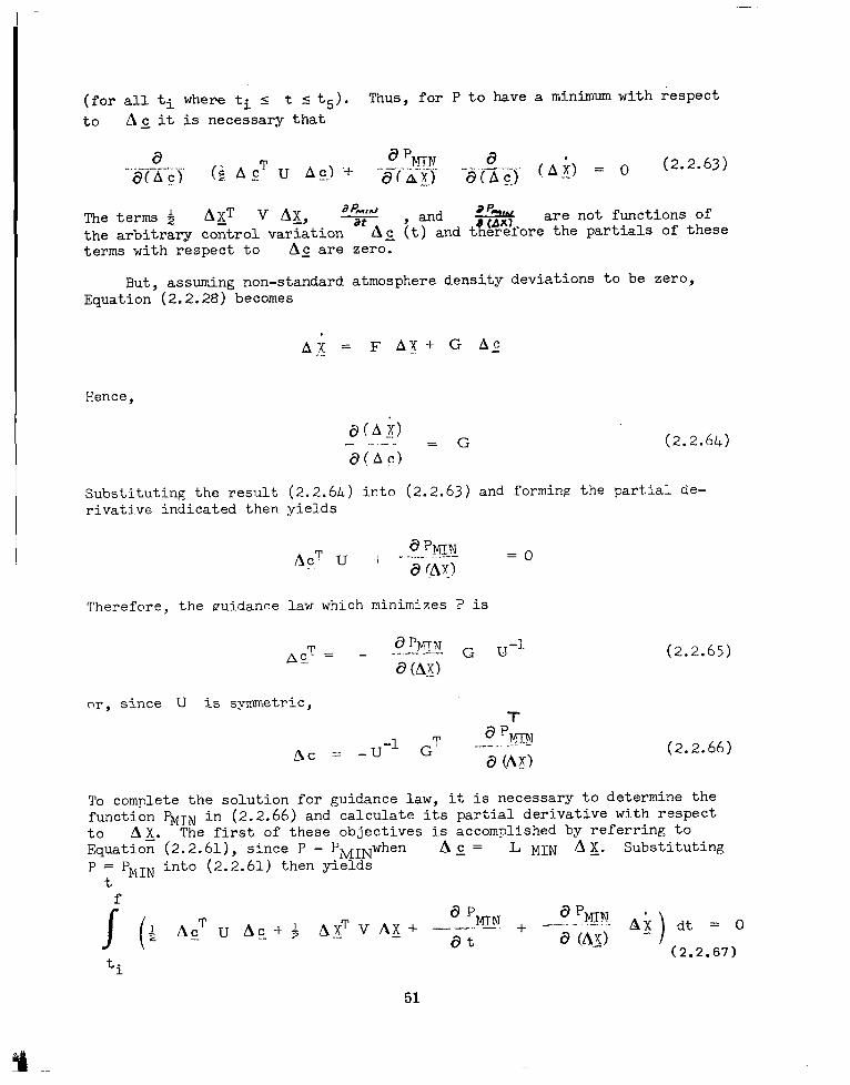
(for all ti where ti 5 t I ts). Thus, for P to have a minimum with respect to AC it is necessary that

a (5 A_cT u A g-1 ‘+

a pM-rhT ^.--_- --... . .-- _.._~ ._.. ___.._- iStAG, a(&. CAi) = 0 a%?) _. (2.2.63)

The terms 8 A&T V Ax, + , and 3 fL*L the arbitrary control variation As (t) and t k!-%ore R

are not functions of the partials of these

terms with respect to AC are zero.

But, assuming non-standard atmosphere density deviations to be zero, Equation (2.2.28) becomes

A,; = F Ax + G A:

Hence,

(2.2.64)

Substituting, the result (2.2.64) into (2.2.63) and forming the partial derivative indicated then yields

bc TU + - !%!LN = 0 a (A)0

Therefore, the puidance law which minimizes P is

d plulTr\T A&c = _ ----A- G u-1.

6’ (AZ)

or9 since U is symmetric, T

-1 GT a ?pf-Iy AC = -u

6’ (.A@

(2.2.65)

To complete the solution for guidance law, it is necessary to determine the function PMIN in (2.2.66) and calculate its partial derivative with respect to A&. The first of these objectives is accomplished by referring to Equation (2.2.61), since P - PMINwhen AC = L MIN AZ. Substituting ' ; 'MIN into (2.2.61) then yields

f

I( h AT u A?-+$ AxT V A1[+ a PMTN __ -.. _ + --.-

at

ti

51

-

But Equation (2.2.67) must be satisfied for all values of ti, thus %IN is determined by the condition that the integrand of (2.2.67) must be zero for

L = L IqIN"9 i.e.,

_ ..,f pm ap

A :,T u A g + 4 A?J'VA;r+ &---. -t ?JTN

+. -- -.- -._ Ai = 0 (2.2.68)

d (Ayl

To solve (2.2.68), Kovatch suggested a solution of the form;

P MT?!

I Ax 't), t, tc) = i AxT (t) A .p (t, t.J Ax (t) (2.2.69

where Ap is a 6 x 6 matrix having time-varying elements. This form is also suggested by the minimum msan square control deviation solution of (2.2.3.4). Assuming this solution

a ‘WIN . -. - - = AK~ hp (2.2.70) a !Ag

= ;. (A li’ FT + AcT GT 1 Ap A\‘< + $ AXT ii, Ais +

$ A$ A, (FAX_ +GAc? (2.2.71)

-------------------_------------------- ':-The proof of this is omitted here

52

Now, substituting (2.2.70) into (2.2.65) and (2.2.66) then gives

? -1 AC = - Ax: Ap G u (2.2.72a)

-1 C = - u G’ APT Ax

Thus, Fquation (2.2.71) can be written as

(2.2.72b)

-1 = $ A&,' A, -2A GU GT APT + lip + AD~J Ax

P

(2.2.73)

At this point the terms in (2.2.68) are expanded as

d h-rw .- _-& d (Ah)

A,: = AxT Ap (FAX +GAc-)

=AXT , A,FA~- Ar' A., G U--l- G' A Ax P

= AFT! Ah

(2.2.74)

53

-1 2 AcTU &=i(AZJT ApG U-l) U (U GT ApT Ax)

$ A$( A -1 T

= PGU G APT, A11 (2.2.75)

Now,if the expressions (2.2.73), (2.2.7&), and (2.2.75) are substituted into Equation (2.2.68), the result is

1 2 AzT ( FT A. -3ADG U-'GTAPT+Ap+3ApF + v)Ac=O

P .

But for this relation to be satisfied for all values of A&, the expression in the parentheses in (2.2.76) must be zero. That is,

d AD -A = - FT A +3/l G U-lGTAT dt P ? P

- 3 Ap F - V (2.2.77)

Finally, the guidance law which minimizes the performance measure P is given by

AC (t) = - U-l GT A T A X (t) P

(2.2.78a)

where A is the solution of the system of differential equations given by (2.2.77) aRd having a boundary condition for Equations (2.2.68) and (2.2.69), i.e.,

Ap determined from

I A .c (t, tf)

=T

(2.2.78b)

t=t f

2.2.3.6 The Velocity-Dependent Approach

The linear perturbation guidance laws presented in previous sections employ time as their independent variable and the look-up variable in the tabulation of the gain matrix in the system's mechanization because the equations of motion are written using time derivatives. The selection of time as the independent variable is appropriate for space guidance where time of arrival is often an important factor. For entry guidance, however, the time of arrival often is unimportant and the use of other independent variables may be investigated. The use of velocity for entry guidance is especially appropriate since:

. The velocity magnitude is often a good indicator of ranging potential and is intimately involved in specifying the flight limits.

54

. The aerodynamic characteristics of the vehicle can be approximately determined as functions of the relative velocity.

However, to use velocity as an independent variable, all time derivatives in the equations of motion must be multiplied by the inverse of the expression for dV/dt. This multiplication is valid as long as dV/dt # 0. In addition, all time-dependent forcing functions, such as the aerodynamic control vector, must be transformed. In this fashion, the equations of motion can be written in the form

(2.2.79)

where z is a column vector having five components, (i.e., one less than the state vector), and where the vector function zv is dependent on z, the aerodynamic control vector 2, (now a function of velocity), and the velocity. The vector z is dependent on all components of the position vector and two components of the velocity vector, (the third component was eliminated by the transformation). However, it is noted that the dependence may involve intermediate functions. Some examples of Z vectors which qualify for the velocity dependent approach to linear perturbation guidance are given by:

h

z = z

=

( ) 2 m

R

Y

cl lb

Starting with the vector set of equations (2.2.791, two linear guidance laws using velocity as the indepent variable can be developed in exactly the same manner of Sections (2.2.3.4) and (2.2.3.5). The development of these theories need not be repeated. By eliminating one variable from the development, the differential equations used to determine optimum guidance gains will contain one less variable and therefore will be somewhat simpler to integrate. How- ever, the form of the linear perturbation guidance law will remain

AC = Lv AZ (2.2.82)

where the gain matrix, L v,is velocity-dependent. Since the velocity-dependent approach to linear guidance adjusts the trajectory control to a variable more closely related to entry performance than time, this approach should be used if a nominal trajectory approach to entry guidance is selected.

55

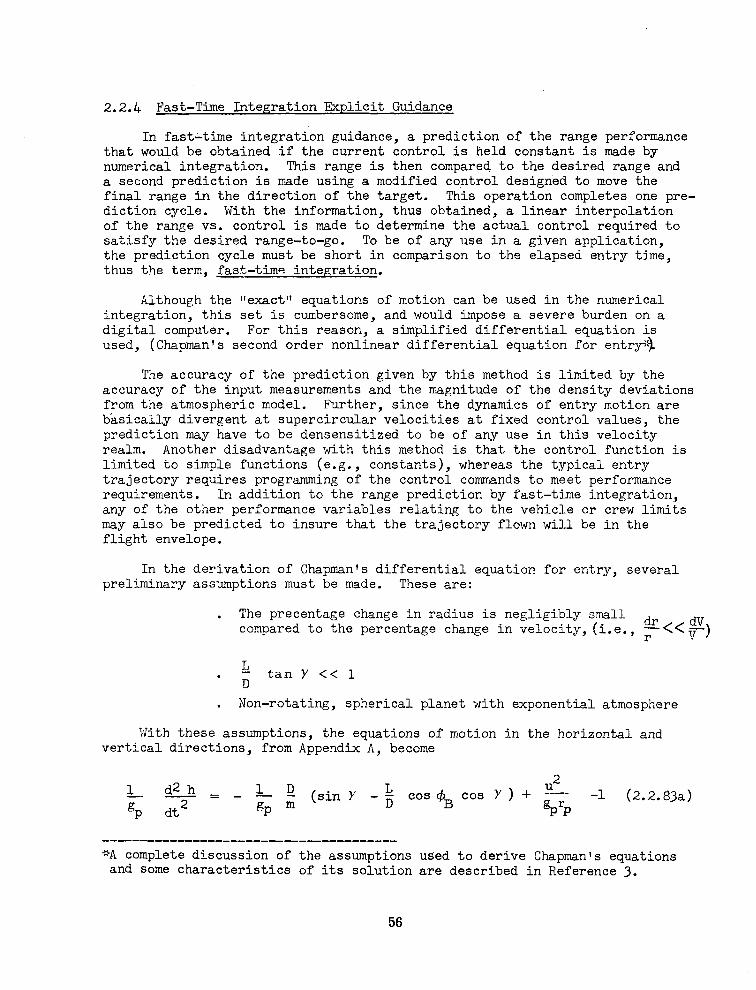
2.2.4 Fast-Time Integration Explicit Guidance

In fast-time integration guidance, a prediction of the range performance that would be obtained if the current control is held constant is made by numerical integration. This range is then compared to the desired range and a second prediction is made using a modified control designed to move the final range in the direction of the target. This operation completes one prediction cycle. With the information, thus obtained, a linear interpolation of the range vs. control is made to determine the actual control required to satisfy the desired range-to-go. To be of any use in a given application, the prediction cycle must be short in comparison to the elapsed entry time, thus the term, fast-time integration.

Although the ['exact" equations of motion can be used in the numerical integration, this set is cumbersome, and would impose a severe burden on a digital computer. For this reason, a simplified differential equation is used, (Chapman's second order nonlinear differential equation for entry:9

The accuracy of the prediction given by this method is limited by the accuracy of the input measurements and the magnitude of the density deviations from the atmospheric model. Further, since the dynamics of entry motion are basically divergent at supercircular velocities at fixed control values, the prediction may have to be densensitized to be of any use in this velocity realm. Another disadvantage with this method is that the control function is limited to simple functions (e.g., constants), whereas the typical entry trajectory requires programming of the control commands to meet performance requirements. In addition to the range prediction by fast-time integration, any of the other performance variables relating to the vehicle or crew limits may also be predicted to insure that the trajectory flown will be in the flight envelope.

In the derivation of Chapman's differential equation for entry, several preliminary assumptions must be made. These are:

. The precentage change in radius is negligibly small compared to the percentage change in velocity,(i.e.,

4 . tan Y << 1 D

. Non-rotating, spherical planet with exponential atmosphere

With these assumptions, the equations of motion in the horizontal and vertical directions, from Appendix A, become

1 d2 h 1 L U2 - = - -

Rp &2 El

gp m (sinY -jj cos c$$ co9 Y > + -

VP -1 (2.2.83a)

------------------------------------ -%A complete discussion of the assumptions used to derive Chapman's equations

and some characteristics of its solution are described in Reference 3.

56

du L-! dt = - m

cos l Y = - ; CDS U2

m cos Y (2.2.83b)

However, it was found by Chapman, that the adaption of a new independent variable,

and a new dependent variable,

CDS r,S z =$y- -

(2.2.84)

would permit Equations (2.2.83a, b) to be replaced by a single differential equation which is nonlinear and of second order in Z . The solution of this equation is called the Z function by Chapman. From (2.2.84), this function is seen to be proportional to the free-stream Reynolds number history of the flow, (if atmospheric viscosity is assumed constant).

The predicted flight path angle history is determined by forming the derivative of (2.2.84) with respect to the independent variable u to yield

(2.2.85b)

where (-pp ) is substituted for dp /dh, and u tan Y is substituted for (dh/dt). But this equation can be solved for the sine of the flight path angle. Thus,

1 dZ - Z sinY =

pd rp6 z E-- (2.2.86)

57

This expression, in turn, can be substituted into the nondimensional acceleration Equation (2.2.8ja) to give

. 1 d2h _ - - - g dt2

cos $ cos Y

vertical

+ii2-1 .

(2.2.87)

to yield,

(2.2.83b), and (2.2.84) were used in substituting for (D/m) in Equation (2.2.83a). Another expression for the non-

acceleration can be obtained by differentiating u tan Y

1 d2h-1 d E-

- - - dt (U tanY) = k ( 2 tan Y+USSC2Y g)

P dt2 gP

'uz d2 z

= 1 -cos2+ + Gtan2Y T-7 - u

Since

dY = dY dii dt due dt

1 = -- co9 Y $ tp$ [:, (2 - :)I(- e,i 1 +) (2.2.82)

and

du UZ dt =

- gp$ Pi cos Y (2.2.90)

Thus, equating the right hand sides of Equations (2.2.87) and (2.2.88) and substituting the expression (1 - sec2 Y ) for (tan2 Y ) the Chapman second order non-linear differential equation for entry is obtained, i.e.,

d2 Z dZ Z 1 -2 -u AL - + - = d z2 d; U iiZ

cos4y -pf rpc 3 cos $ cos3 (2.2.91)

58

where, the cosine of the flight path angle is found by (2.2.91)

COSY = [l- &-- (L.$ _ $]$

Finally, the longitudinal and lateral ranges are obtained by solving the following

where

equations:

t f =

I +

cos Y cos $h du

Z (2.2.92)

cos Y sin $5 (2.2.93)

Z dii

cos$ cos Y tan ( Pi 1

Z p’ rp 3 du (2.2.94)

u- 1

A list of other performa;ce variables predicted in terms of the Z function and the velocity ratio u, is available in Reference 3.

The initial step in the prediction cycle requires the computation of the initial value of Z and dZ/du. These initial values are found as a function of the initial drag acceleration and altitude rate, from (2.2.84), and (2.2.85) as 1

( ) rpZ CDS zi=-- - B s m

P ui

kprp) h

( ) i! 1 m. 1 = a

(9,014 ui

2 cos Yi

(2.2.95)

59

+ ( p rp)? sin Yi, (2.2.96)

tan Yi= 2 u. 1

Prediction of the ranpe performance usinls fast-time integration is now accomplished by numerical intepration of the Eauations (2.2.91), (2.2.93) and (2.2.93) subject to the initial conditions piven by (2.2.95) and (2.2.96).

60

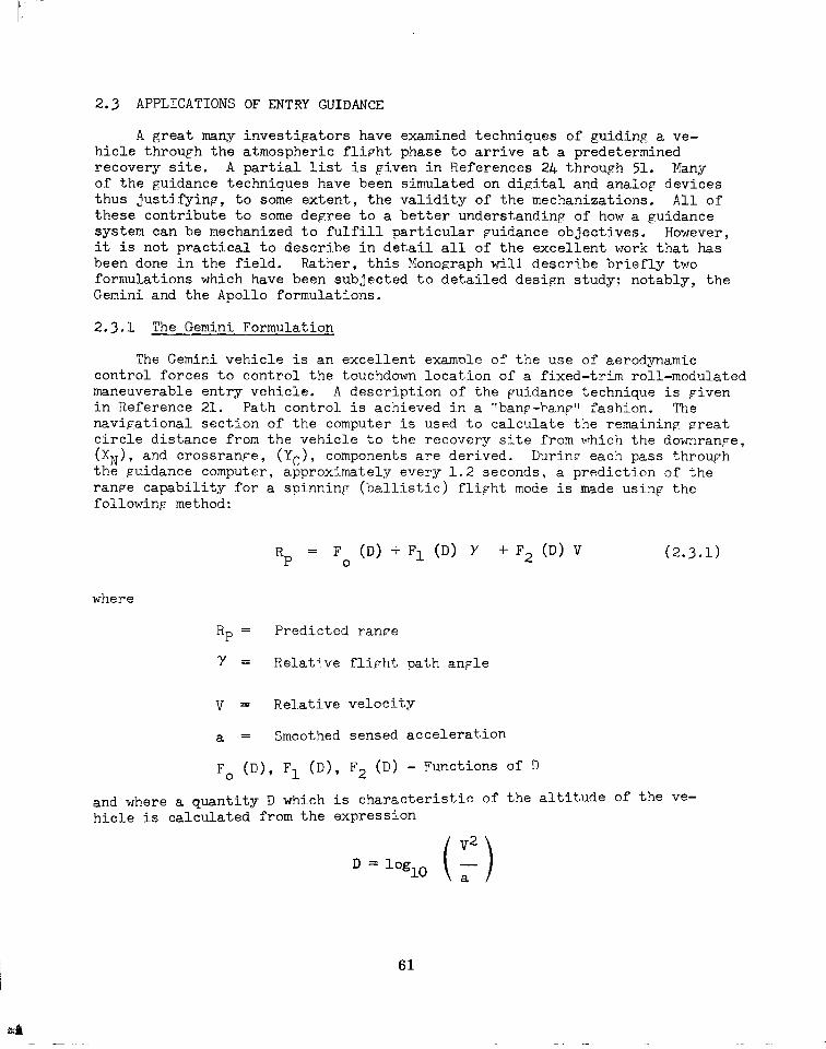
2.3 APPLICATIONS 0~ ENTRY GUIDANCE

A great many investigators have examined techniques of guiding a vehicle through the atmospheric flight phase to arrive at a predetermined recovery site. A partial list is piven in References 24 throuph 51. Kany of the guidance techniques have been simulated on digital and analog devices thus justifying, to some extent, the validity of the mechanizations. All of these contribute to some degree to a better understanding of how a guidance system can be mechanized to fulfill particular @dance objectives. However, it is not practical to describe in detail all of the excellent work that has been done in the field. Rather, this Monograph will describe briefly two formulations which have been subjected to detailed design study: notably, the Gemini and the Apollo formulations.

2.3.1 The Gemini Formulation --

The Gemini vehicle is an excellent example of the use of aerodynamic control forces to control the touchdown location of a fixed-trim roll-modulated maneuverable entry vehicle. A description of the puidance technique is Fiven in Reference 21. Path control is achieved in a "bane-banp" fashion. The navigational section of the computer is used to calculate the remaininp preat circle distance from the vehicle to the recovery site from which the downrange, (x,) 9 and crossranpe, (Yc), components are derived. DurinF each pass throuph the guidance computer, approximately ever.y 1.2 seconds, a prediction of the ranFe capabilitg for a spinninF (ballistic) flipht mode is made usinp the followinp method:

RP = F (D) + Fl (D) Y + F2 (D) V

0 (2.3.1)

where

Rp = Predicted range

Y = Relative flight path angle

V = Relative velocity

a = Smoothed sensed acceleration

F. (D), Fl (D), F2 (D) - Functions of D

and where a quantity D which is characteristic of the altitude of the vehicle is calculated from the expression

61

The vehicle is caused either to roll at a constant rate or to maintain a bank attitude depending upon the relationships between Rp, XN, and Yc. If Rp c Xp;, a constant snin rate is commanded providing Y calculated limit.

is less than a specified or Otherwise, a bank angle of 90" is commanded which will turn

the vehicle toward the recovery site. If Rp 4 XN, a lift attitude is commanded based upon the relative values of Yc and XN.

A bal1ist.j.c flipht mode was selected as the basis for ranBe prediction because it was felt that the uncertainties in the drap parameter would be less and that the predicted value of ranfre would be better than if the lift parameter was also employed. To prevent a tarret overshoot, Rp was biased to cause an early spin. The bias was removed as the vehicle approached the recovery site. Thouph this method results in Food ranFinEr accuracy, one of the shortcominFs is the radically different command attitude state which may result. For example, the vehicle may just reach its maximum roll rate when a constant bank anple is commanded. Then, the reverse may happen resultinp in inefficient attitude control fuel usage. A simple fix is to eliminate the spin command and replace it with a 90" bank anf;le command.

Another method of longitudinal control is that described in Reference 22. This method is fundamentally th e same as that employed for Apollo in the termi.nal Flide phase. The theory of this method is Fiven in Section (2.2.2). The control equation which yields the commanded vertical plane L/D is

( k)c =( ika + K4 cy - y& + K5(i - 9a,, + k (R - RREF) (2.32)

where (L/D>R~, ‘RFF, D/m~~F and RREF define the reference trajectory characteristics as a functionof velocity, and Kq, K , and K6 are sensitivity coefficients as a function of velocity compatible wi z h the reference trajectory, The coefficients can be obtained throuph solutions of the adjoint equations and/or emperically from traiectorg simulations. The error terms are not necessarily restricted to those shown. For example, any term indicative of enerpy dissipation could be used in lieu of D/m. And any other term indicative of the rate of chanfre of enerFy dissination could be used in lieu of

Y . Likewise, any monotonicallg chanfinr parameter could be used as the independent variable in place of veloci_ty. The selection of these parameters is dependent upor, the sensor capabilities and the Fuidance reauirements. This method is not restricted to a fixed-trim roll-modulated vehicle. For example, omc may represent an anple-of-attack requirement. The ranpin~ accuracy of this method is also excellent when applied as described since closeness to the reference trajectory can be expected. Fntri.es from reduced velocities, such as from a boost abort"', l,,rithout selection of a new reference trajectory will tend to reduce the accuracy because of the linear assumptions. The mechanization is straiphtforward although storage of six parameters as a fllnction of the independent variable is required.

62

2.3.2 The Apollo Formulation

An example of entry Fuidance from supercircular entry conditions is that of the Apollo eiven in Reference (23). The Apollo system combines features of both the explicit and implicit techniaues. The complete puidance logic is extremely complex invnlvinp many lopica decisions and solutions to many equations. Therefore, only the essentials of the Puidance law are described startinp v6th downranpe control.

At the start of the initial entry phase, a lopical decision to select a lift-u? or lift-down attitude is made based upon an imperical relationship which defines the position w5thin the corridor. Another lopical decision, based upon sensed acceleration is reauired to terminate a lift-down command: the initial entry phase is terminated and the transition phase is initiated near the maximum G point upon reachinp a specified negative altitude rate.

The calculations performed and the vehicle attitude commands derj.ved durinr the transition phase are the key to successful rancinp from supercircular velocities. The vehicle is initially maneuvered to a specified acceleration level using errors in acceleration and altitude rate as a control base. As the vehicle traverses this path, a range prediction is made every two seconds. The ranpe prediction is achieved by summinp the following components: (I.) ranpe from the vehicle to the atmospheric exit point, (2) ranpe along a draF free Keplerian arc, and (3) ranpe durinp the second entry. The predicted ranpe is compared with the remaininp ranpe-to-F0 durinp each pass throu,Fh the guidance computer. When the tT.70 are approximately equal., a reference path for which the predicted ran-e eouals the remaininp range-to-pr w5.thj.n a small. tolerance is selected by an iterative procedure. The vehicle is then controlled to the reference path until exit occurs. Vhile the vehicle is abcve the sensible atmosphere, the vehicle's pitch and roll attitudes are adjusted to appropriate values for initiation of the second entry (re-entry). The re-entry path is traversed usinp an implicit puidance method usinp errors in range, D/m, and altitude rate as a base velocity bejnp the independent varjable.

The path from the vehicle's present position to the atmospheric exit point is de.fined explicitly on the basis of a constant value of L/D somewhat less than the maximum value to provide a reserve for vehicle control. The assumptions involved durinp the derivation of the pull up to exit path result in a reference path which does not match the path that would be obtained by snlvinp the complete equations of motion. However, the path is an adequate approximation and, what is more important, yields a nath that can be flown

;kAn open-loop control approach is usually sufficient for this case.

63

and described analytically. The key to the derivation is the relationship between altitude rate and velocity which is approximately correct in the neighborhood of circular.velocity where the v2/, - g term may be assumed to be zero. This approximate relationship

;2 - 4 = $ (Vi -v2) (2.33)

. can be used to relate h and c at any two points on the reference path. Other approximate explicit relationshi.ps .are used to relate velocity alonp the path to the acceleration level. These relations permit definition of V and h as a function of acceleration alonp the path. Thus, taking the acceleration level as zero, permits calculation of the ve1ocit.y and altitude rate at the exit point necessary for the calculation of the predicted ranre components. The range-tc-exit is based upon an explicit relationship in- volvinp the reference path terms. The second entry ranpe is predicted based uron a linearization of precomputed values of range vs velocity for a specified entry path anple plus a correction to account for a variation in entry path anele.

%or some values of reouired entry range, an atmospheric exit is not required but a transfer to a low acceleration level is required. For this condition, as the vehicle traverses the constant acceleration oath, the predicted rat-q-e will decrease until fina1i.y the KeFlerian arc ranpe reduces to zero. If, at this point, the predicted ranFe still exceeds the ramaininp range to go, the method of predicting range is adjusted to predict the minimum acceleration level that can be achieved with a constant L/D pull-up. Then, the predicted ranpe components then consist of (1) ranpe to the minimum G point and (2) ranpe from the minimum G point to touchdown, both ranges beinp calculated as before. Frhen the predicted range eauala the remaininp ranpe to go. the reference trajectory to the minimum G point is selected, the vehicle is controlled to this reference until a ncpative altitude rate occurs which sicnifies that the minimum G has been reached, and the remaining ranpe in the terminal plide repion is then controlled usinp the implicit method previously mentioned. If the required entry rarqe is shorter yet, that is, the predicted velocit y at the minimum G point is less than some limiting value, control is transferred directly to the implicit terminal Flide calculations.

Control along the reference trajectory either to the atmospheric exit point or to the minimum G point, whichever is appropriate, uses acceleration level as the independent variable from which reference values of velocity (VR~~> and altitude rate (hp,EF> are calculated. Deviations in velocity and altitude rate from the reference values are used as a control base. The control fains are adjusted to Five more weipht to velocity errors than h errors as the exit or minimum G points are approached.

A precomputed reference trajectory is used in the terminal Flide phase which is representative of mean terminal Flide motion. The reference is based upon a positive value of L/D which Fives approximately equal range correction capability in each downranFe direction. Reference values of range,

64

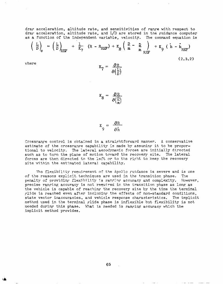
drap: acceleration, altitude rate, and sensitivities of range with respect to drap acceleration, altitude rate, and L/D are stored in the Guidance computer as a function of the independent variable, velocity. The command ea.uation is

(2.3.2) where

CrossranFe control is obtained in a Straightforward manner. A conservative estimate of the crossranpe capability is made by assuming it to be proportional to velocity. The lateral aerodynamic forces are initially directed such as to turn the plane of motion tcrGrard the recovery site. The lateral forces are then directed to the left or to the right to keep the recovery site within the estimated lateral capability.

The flexibility reouirement of the Apollo Fuidance is severe and is one of the reasons explicit. techniques are used in the transition phase. The penalty of providing flexibility is ranpine accuracy and complexity. FIowever, precise ranping accuracy is not required in the transition phase as lonp: as the vehicle is capable of reaching the recovery site by the time the terminal plide is reached even after includinp the effects of non-standard conditions, state vector inaccuracies, and vehicle response characteristics. The implicit method used in the terminal Flide phase is inflexible but flexibility is not needed durinp this phase. What is needed is ranpinp accuracy which the implicit method provides.

65

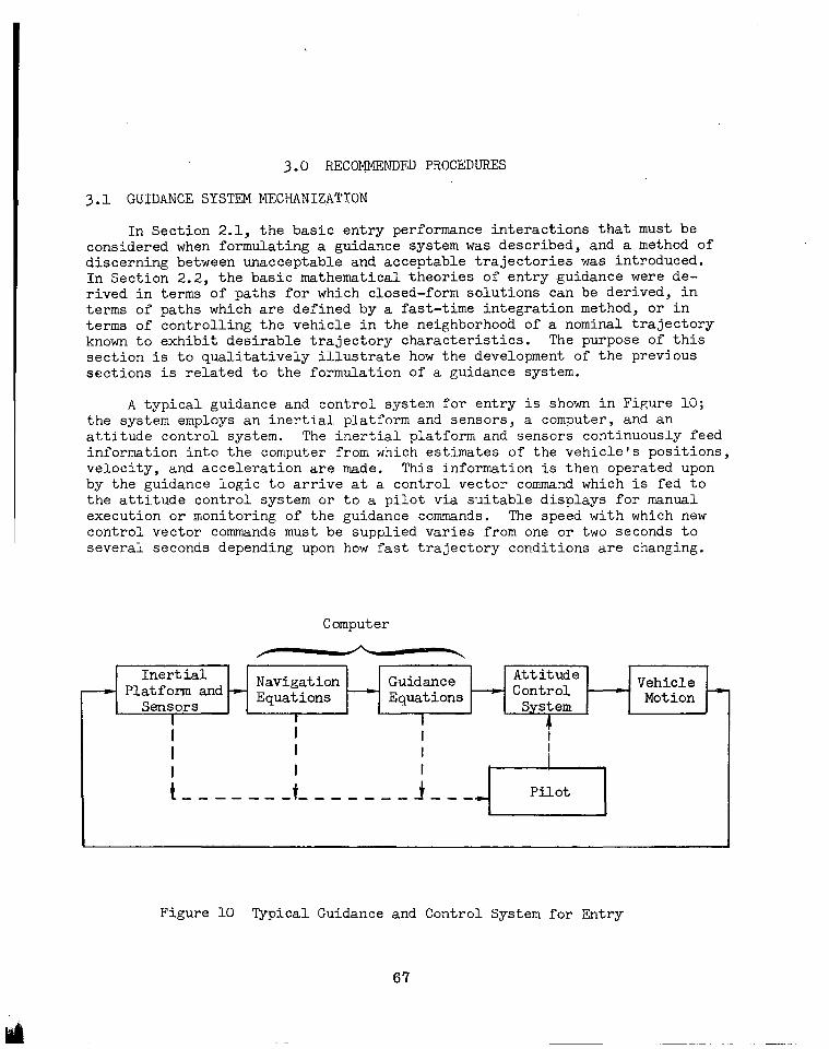
3.0 RECOMMENDED PROCEDURES

3.1 GUIDANCE SYSTEM MECHANIZATION

In Section 2.1, the basic entry performance interactions that must be considered when formulating a guidance system was described, and a method of discerning between unacceptable and acceptable trajectories was introduced. In Section 2.2, the basic mathematical theories of entry guidance were derived in terms of paths for which closed-form solutions can be derived, in terms of paths which are defined by a fast-time integration method, or in terms of controlling the vehicle in the neighborhood of a nominal trajectory known to exhibit desirable trajectory characteristics. The purpose of this section is to qualitatively illustrate how the development of the previous sections is related to the formulation of a guidance system.

A typical guidance and control system for entry is shown in Figure 10; the system employs an inertial platform and sensors, a computer, and an attitude control system. The inertial platform and sensors continuously feed information into the computer from which estimates of the vehicle's positions, velocity, and acceleration are made. This information is then operated upon by the guidance logic to arrive at a control vector command which is fed to the attitude control system or to a pilot via suitable displays for manual execution or monitoring of the guidance commands. The speed with which new control vector commands must be supplied varies from one or two seconds to several seconds depending upon how fast trajectory conditions are changing.

Computer

Inertial 1

Navigation Guidance Attitude gr Platform and *

Sensors Equations - Equations - Control _ Vehicle

System Motion -

Figure 10 Typical Guidance and Control System for Entry

67

3.1.1 Guidance of a Vehicle having a Single Control Variable

This section is concerned with guidance of a vehicle having a single control variabls such that the aerodynamic force components in the trajectory plane (vertical plane containing the velocity vector) and normal to the trajectory plane (lateral) can be varied. A fixed-trim roll-modulated vehicle has this characteristic. For such vehicles, the vertical plane and lateral force components are coupled; i.e., only one component of the force requirements can be satisfied at any particular time. However, it will be shown that force requirements in the vertical plane are generally the most critical with respect to fulfilling ranging objectives.

The fundamental technique used for guiding this type of vehicle to a desired landing site can be illustrated by considering the footprint which contains all possible points which can be reached for specified vehicle aerodynamics and state vector. Consider the representative footprint illustrated in Figure 11 at some arbitrary time during entry in a non-rotating planet atmosphere. The axis of symmetry is defined by the vertical plane containing the position and velocity vectors at the given time. The heavy line illustrates the ground trace that would be traversed by the vehicle for a specified vertical plane force schedule with the residual lateral forces always directed to the right. The light trajectory traces illustrate the variation in the touchdown position that can result if the direction of the lateral forces (same vertical plane force schedule) is reversed at various points along the originally described trajectory trace. The distance along all arcs is the same. Assume that the direction of the lateral forces can be reversed as frequently as desired. A variety of paths could then be drawn which would all terminate at the same point. In the limit, the vehicle could be turned until the instantaneous trajectory plane contained a desired recovery site and by rapidly reversing the direction of the residual lateral forces (bank angle reversals), the vehicle could remain in this plane until arriving at the desired recovery site.

68

/

Arbitrary Trajectory Point,

Crossrange-

Figure 11 Effects of Lateral Force Direction Reversal on Touchdown Position for a Vehicle having a Single Control Variable

Note: The aerodynamic force schedule in the plane of the trajectory is identical for all the ground traces shown. The schedule of the residual force normal to the trajectory is likewise the same in magnitude; its direction, however, is reversed once at various times during the flight.

69

Guidance to a specified recovery site can thus be achieved by considering two uncoupled tasks: (1) control of the vertical plane forces to give a desired arc length (longitudinal ranging), and (2) reversal of the residual lateral forces such that the plane of the trajectory contains or is within an allowable tolerance of the recover site (lateral ranging). The guidance computer would thus have three essential functions as shown in Figure 12.

LONGITUDINAL

1 RANGING

Figure 12 Guidance Computer Functions

The navigational function defines the vehicle state and calculates the arc length from the vehicle to the recovery site for use in the longitudinal ranging section of the computer. If the vehicle aerodynamics and its energy level are such that the cross-range capability is much smaller than the downrange capability, an adequate approximation to the required arc length, RTGJ can be calculated as the great circle distance from the vehicle to the recovery site. If the cross-range is of the same order of magnitude as the downrange, the great circle approximation yields too small an estimate. For this condition, some technique must be devised to estimate the length along the arc the vehicle will fly in reaching the recovery site.

An example of guidance to a specified recovery site is illustrated in Figure 13.

70

Unprimed Letters Denote Position of the Vehicle and Points at Which the Direction of the Lateral Forces are Reversed.

Primed Letters Denote the Size of the Footprint Correkponding to Each Unprimed Letter.

--Recovery Site

r’ ^ Arbitr ary Trajectory Point

;:A

Crossrange-

Figure 13 Convergence of Footprints around Recovery Site

71

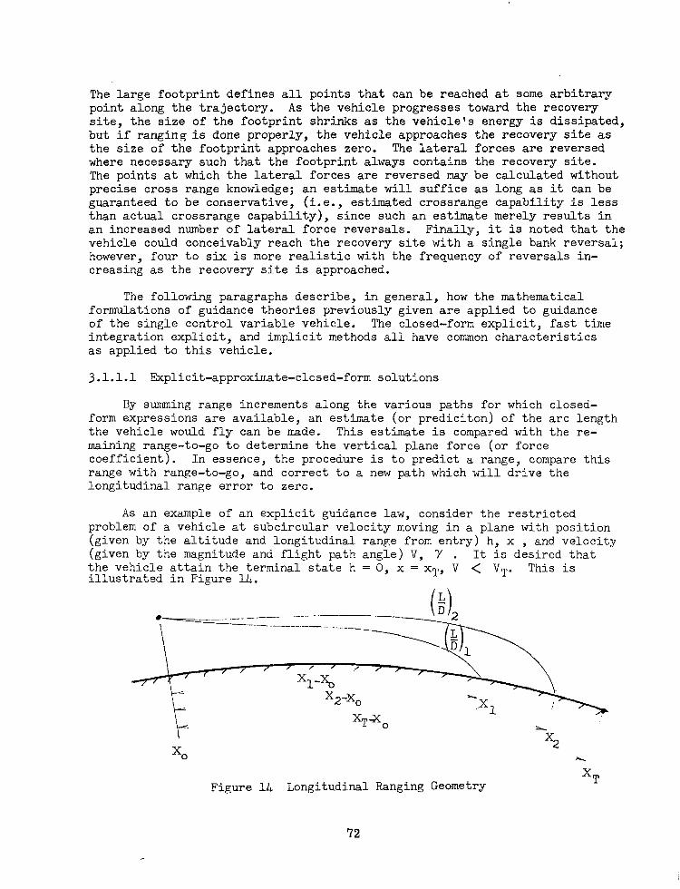
The large footprint defines all points that can be reached at some arbitrary point along the trajectory. As the vehicle progresses toward the recovery site, the size of the footprint shrinks as the vehicle's energy is dissipated, but if ranging is done properly, the vehicle approaches the recovery site as the size of the footprint approaches zero. The lateral forces are reversed where necessary such that the footprint always contains the recovery site. The points at which the lateral forces are reversed may be calculated without precise cross range knowledge; an estimate will suffice as long as it can be guaranteed to be conservative, (i.e., estimated crossrange capability is less than actual crossrange capability), since such an estimate merely results in an increased number of lateral force reversals. Finally, it is noted that the vehicle could conceivably reach the recovery site with a single bank reversal; however, four to six is more realistic with the frequency of reversals increasing as the recovery site is approached.

The following paragraphs describe, in general, how the mathematical formulations of guidance theories previously given are applied to guidance of the single control variable vehicle. The closed-form explicit, fast time integration explicit, and implicit methods all have common characteristics as applied to this vehicle.

3.1.1.1 Explicit-approximate-closed-form solutions

By summing range increments along the various paths for which closed- form expressions are available, an estimate (or prediciton) of the arc length the vehicle would fly can be made. This estimate is compared with the remaining range-to-go to determine the vertical plane force (or force coefficient). In essence, the procedure is to predict a range, compare this range with range-to-go, and correct to a new path which will drive the longitudinal range error to zero.

As an example of an explicit guidance law, consider the restricted problem of a vehicle at subcircular velocity moving in a plane with position (given by the altitude and longitudinal range from entry) h, x , and velocity (given by the magnitude and flight path angle) V, Y . It is desired that the vehicle attain the terminal state h = 0, x = XT, V < VT. This is illustrated in Figure 14.

l - _.. .-- - --- _--.--

-- ---- --.- _,.__

<

I

X0 *

Figure 14 Longitudinal Ranging Geometry

72

I

Disregarding, for purposes of illustration, the fact that the trajectory flown by the vehicle must be restricted within the configuration's acceptable flight regime, the objective of the guidance system is to command an in-the- plane-of-motion lift/drag ratio to guarantee that the terminal conditions are met. For simplicity, assume that constant (L/D) is maintained for the remaining duration of the flight.. Under these conditions, an explicit guidance scheme predicts the terminal range for two or more fixed values of (L/D); then with this information and the knowledge of the desired terminal conditions, the scheme selects a command value of (L/D). denote the terminal ranges predicted for a vehicle Y > and having fixed values of lift/drag ratio given by spectively. One means of defining the proper L/D is to employ a guidance law linear in the difference between the predicted and desired boundary values. In such a.system, the desired L/D can be calculated by first expanding the terminal range function of (L/D) in a Taylor series about a predicted value Xp, i.e.,

x, = xp * (3.1.1)

where the large parentheses mean "evaluated at". Thus, approximating the derivative by the ratio of finite differences,

(3.1.2)

and assuming terms in (3.1.1) of second and higher order are negligibly small, allows the command (L/D) to be calculated from (3.1-l) and (3.1.2) as follows

= (3.1.3)

COMMANQ

In order for this explicit guidance law to be effective, it is necessary that the predicted values of range be sufficiently close to the desired value that the linear approximation is good. However, since the vehicle's exit from the atmosphere could interfere with the validity of the linear approximation, entry guidance laws of this form are not used for trajectories having segments both in and out of the atmosphere. Thus, if employed, provision must be made in the guidance logic to override a guidance law when it is in danger of becoming invalid, (that is, when the state of the vehicle at any point along the predicted path, including the initial point,, is not within the configuration's acceptable flight regime).

73

3.1.1.2 Explicit-Fast-Time-Integration

The application of fast time integration accomplishes the guidance task in much the same way as the closed-form methods with two exceptions: (1) the touchdown position is calculated in addition to the arc length and (2) additional parameters such as load factor,. aerodynamic heating rate and heating load which may be critical to flight, can be calculated. The functional operations of this and the preceding theory are essentially the same.

3.1.1.3 Implicit

The implicit method can be made to resemble either of the two previous methods. If only the vertical plane characteristics of the reference trajectory and associated sensitivity coefficients are stored, the implicit method behaves like the explicit-closed-form technique except that the commanded vertical plane control vector is determined directly by relating deviations from the reference to the appropriate sensitivity coefficients. Lateral ranging is accomplished, as before, by reversing the lateral forces to maintain the recovery site within the footprint. If the characteristics of the reference trajectory and associated sensitivity coefficients in the lateral direction are also stored, the implicit method behaves more like the explicit-fast-time-integration technique. Since only one component of the force requirement can be exactly satisfied at any particular time, the longitudinal and lateral force relationships must be weighted to give emphasis to the range error which is predominating.

3.1.1.4 Combinations of Implicit and Explicit Techniques

Each of the three previous techniques described above have limitations which may make it beneficial to combine the good features of each to finalize a guidance law. For example, the closed form solutions are flexible but problems may exist in finding a path which is compatible with the guidance requirement and which also yields an acceptable closed-fo;m solution. The fast-time-integration method gives excellent results but the speed of integration may be too slow compared with the rapidity with which trajectory conditions are changing. The implicit method is very accurate but the vehicle must be constrained to be near the reference which due to uncertainties in the force model and errors in the guidance functions occurring before entry, cannot always be guaranteed.

3.1.2 Guidance of a Vehicle having Multiple Control Variables

The technique of guiding a vehicle having multiple control variables is not fundamentally different (the mathematics and logic are undoubtedly more complex) than guidance of a single control variable vehicle previously described. An example of a vehicle having two control variables is one for which both angle-of-attack and bank attitude are modulated. The availability of two control variables makes it possible to simultaneously satisfy both vertical plane and lateral force requirements. Depending upon the force needs; however, during some phases of the entry it may be necessary to satisfy only one force requirement. This situation would arise whenever force re-

74

111 -

quirements saturate the vehicle's force capability.

The concept of a footprint remains the same and it still is necessary to control two components of range. All guidance theories still apply except that closed-form solutions may not be possible for all paths previously given.

3.2 MISSION AND GUIDANCE PHASES

The missions from which entry guidance may be required are illustrated in Figure 15. Starting from the lower velocities, these missions are (1) entry from boost abort, (2) entry from low altitude Earth orbits or second entry following an atmospheric exit (skip), (3) entry from elliptical Earth orbits, (4) entry from a lunar mission, and (5) entry from planetary missions.

Boost Abort ----

Low Alt. Earth

Planetary _

L .-.. ..-- -.- . ..- ..-.... ._ .-

'CIR

v-

Figure 15 Relationship of Missions to Flight Regime

75

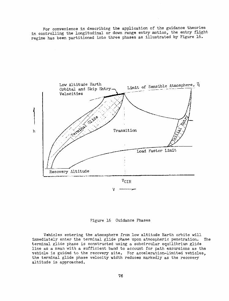
For convenience in describing the application of the guidance theories in controlling the longitudinal or down range entry motion, the entry flight regime has been partitioned into three phases as illustrated by Figure 16.

Low Altitude Earth Orbital and Skip Entry

I Velocities

I

Recovery Altitude I I -.. - .-_-,I_U-

VCIR

v-

Figure 16 Guidance Phases

Vehicles entering the atmosphere from low altitude Earth orbits will immediately enter the terminal glide phase upon atmospheric penetration. The terminal glide phase is constructed using a subcircular equilibrium glide line as a mean with a sufficient band to account for path excursions as the vehicle is guided to the recovery site. For acceleration-limited vehicles, the terminal glide phase velocity width reduces markedly as the recovery altitude is approached.

76

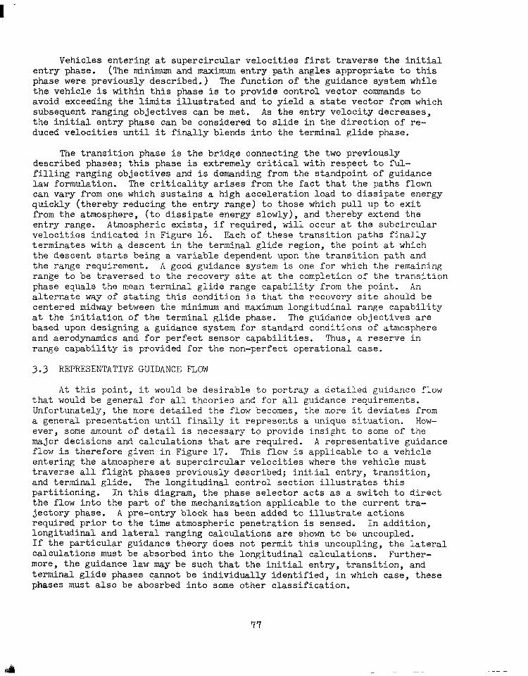
Vehicles entering at supercircular velocities first traverse the initial entry phase. (Th e minimum and maximum entry path angles appropriate to this phase were previously described.) The function of the guidance system while the vehicle is within this phase is to provide control vector commands to avoid exceeding the limits illustrated and to yield a state vector from which subsequent ranging objectives can be met. As the entry velocity decreases, the initial entry phase can be considered to slide in the direction of reduced velocities until it finally blends into the terminal glide phase.

The transition phase is the bridge connecting the two previously described phases; this phase is extremely critical with respect to fulfilling ranging objectives and is demanding from the standpoint of guidance law formulation. The criticality arises from the fact that the paths flown can vary from one which sustains a high acceleration load to dissipate energy quickly (thereby reducing the entry range) to those which pull up to exit from the atmosphere, (to d issipate energy slowly), and thereby extend the entry range. Atmospheric exists, if required, will occur at the subcircular velocities indicated in Figure 16. Each of these transition paths finally terminates with a descent in the terminal glide region, the point at which the descent starts being a variable dependent upon the transition path and the range requirement. A good guidance system is one for which the remaining range to be traversed to the recovery site at the completion of the transition phase equals the mean terminal glide range capability from the point. An alternate way of stating this condition is that the recovery site should be centered midway between the minimum and maximum longitudinal range capability at the initiation of the terminal glide phase. The guidance objectives are based upon designing a guidance system for standard conditions of atmosphere and aerodynamics and for perfect sensor capabilities. Thus, a reserve in range capability is provided for the non-perfect operational case.

3.3 REPRESENTATIVE GUIDANCE FLOW

At this point, it would be desirable to portray a detailed guidance flow that would be general for all theories and for all guidance requirements. Unfortunately, the more detailed the flow becomes, the more it deviates from a general presentation until finally it represents a unique situation. How- ever, some amount of detail is necessary to provide insight to some of the major decisions and calculations that are required. A representative guidance flow is therefore given in Figure 17. This flow is applicable to a vehicle entering the atmosphere at supercircular velocities where the vehicle must traverse all flight phases previously described; initial entry, transition, and terminal glide. The longitudinal control section illustrates this partitioning. In this diagram, the phase selector acts as a switch to direct the flow into the part of the mechanization applicable to the current trajectory phase. A pre-entry block has been added to illustrate actions required prior to the time atmospheric penetration is sensed. In addition, longitudinal and lateral ranging calculations are shown to be uncoupled. If the particular guidance theory does not permit this uncoupling, the lateral calculations must be absorbed into the longitudinal calculations. Further- more, the guidance law may be such that the initial entry, transition, and terminal glide phases cannot be individually identified, in which case, these phases must also be abosrbed into some other classification.

77

As shown, the phase selector during each pass through the guidance logic directs the calculations through the particular part of the logic compatible with the current trajectory phase. In each phase, logical decisions are first required as indicated by the first row of blocks. These decisions answer the questions as to whether or not control should be transferred to the next phase or to some subsection of the current phase. In all cases, a point is always reached where a calculation is performed to determine the vertical plane force requirement. Following these calculations, the direction of the forces is determined by the lateral logic.

3.4 EXPLICIT VS. IMPLICIT METHODS

In each of the three guidance phases (initial entry, transition, and terminal), either explicit or implicit guidance laws can be employed to satisfy the particular requirements of that phase. Both have advantages and disadvantages. For instance, in the initial entry phase, an explicit system has the advantage because of its flexibility in handling the pre-entry initial errors. On the other hand, an implicit system could be employed with advantage during the terminal phase of a supercircular entry mission since its simplicity of mechanization and accuracy are more important factors during this phase than the flexibility factor, the gross ranging task having been accomplished during the transition phase.

By the nature of an implicit scheme, it is obvious that during the transition phase where the family of guided trajectories may encompass a large part of the flight regime, an implicit scheme with a single nominal trajectory does not have the needed flexibility and accuracy to fulfill terminal ranging objectives. Thus, in order to be effective during this phase, more than one nominal trajectory offering some choice in terminal objectives must be employed to provide flexibility. However, the disadvantage of this is that it neglects to capitalize on one of the implicit guidance method's advantages, that of simplicity. Using more than one no.minal not only requires increased storage capacity for the guiding variables and gains, but also demands that a logic be established to decide which of the ttnominalslt is to be the one used.

In summary, some general statements can be made concerning the selection of a guidance theory for any guidance phase. They are:

a> For phases where flexibility of terminal objectives is not a strong requirement and expected initial deviations can be restricted, an implicit approach is generally better.

b) For phases where large flexibility in handling terminal objectives and initial deviations is important, the closed form reference trajectory approach is generally more appropriate.

c> For phases where limited flexibility in handling terminal objectives and the initial deviations can be restricted, an implicit approach employing more than one nominal trajectory should be investigated.

78

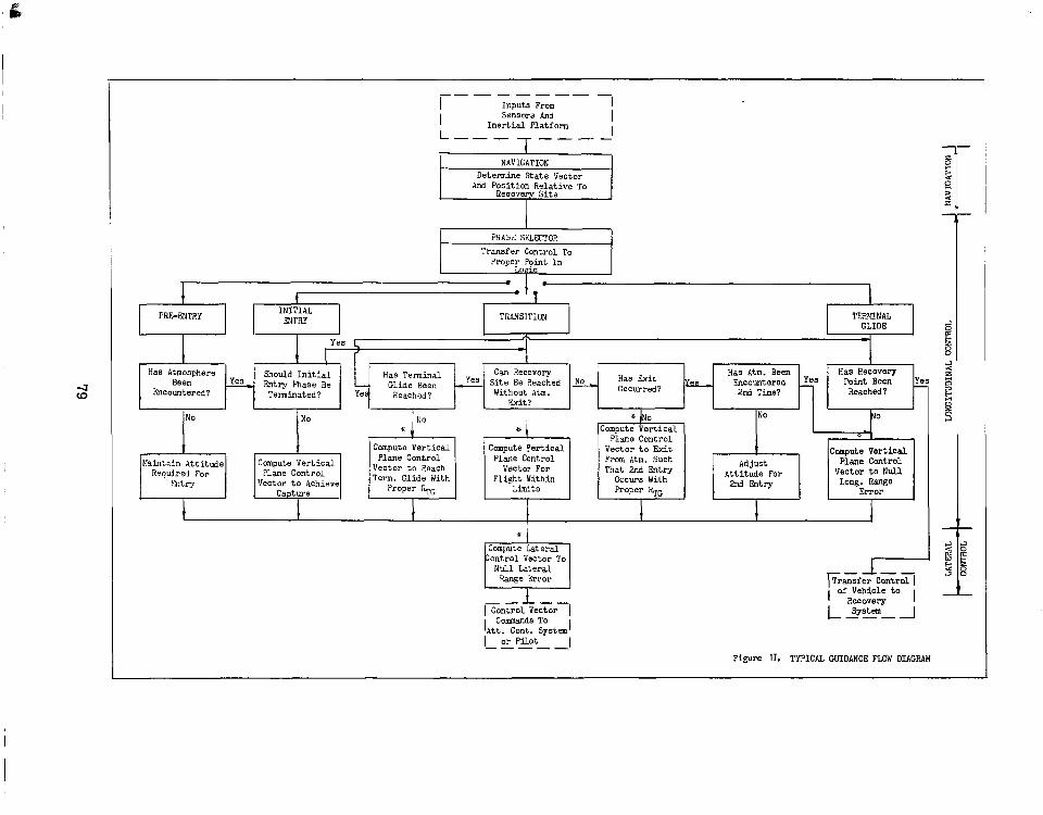
__------- I Inputs From

I Sensors And

Inertial Platform I

L--- ---_I

PHAS:: SZLJZTOR Transfer Control To

Proper Point In oaic

1 PRE-E!J, 1 wwS;:O<--= 1 TE?XNAL GLIDE

Has Atm. Been Encountered

Plane Control Vector to Achieve

* No Compute Vertical

Plane Control vector to Exit From Attm. Such That 2nd Entry

Occurs With hoper qC

I

NO

Adjust Attitude For

2nd Fatly

I

ccapute vertical Plane Control

Vector to Null Long. Range

SiTor

Commands To IAtt. Cont. System

,

or Pilot ----- I Figure 17. TYPICAL GUIDANCE FLOW DIACRAH

d) For phases where large flefibility is desired and the flight conditions are known with high accuracy, a fast-time integration method should be investigated.

e) For flexibility, where the computational limits are not critical the closed form reference trajectory approach is generally best.

However, in comparing the two general classifications of guidance theories with regard to their utility or application a common set of comparison points must be used. These are the following:

. flexibility in handling pre-entry guidance errors and uncertainties

. flexibility in obtaining terminal objectives

. accuracy

. simplicity

. on-board computational requirements

These criteria have been applied in the following table to the various guidance techniques discussed in the text.

Flexibility in Handling Initial Errors and

Uncertainties

Flexibility in Obtainin Terminal Objectives

Accuracy excellent good

Simplicity

On-Board Computational Requirements -__---

Fast-Time Closed Form Inte- Approxi-

gration mation

-~ ~-~~ excellent excellent

excellent excellent

moderate- moderate poor

moderate large I

I

Variable lain Variable Cain Linear Pertur. Linear Pertur.

( S'ingle (Multiple Nominal) Nominal)

___-- good to ext. good to ext.

poor

excellent

excellent

small

limited

excellent

good

moderate

81

The process of finalizing a guidance system depends upon many factors. The content of this monograph is an attempt to consolidate much of the worthwhile information on the subject to aid in guidance system selection. It does not, nor was it intended, to answer all questions with which the guidance system designer will be concerned.

Finally, it is noted that the entry guidance system is only one of the many systems which make up the total vehicle. Thus, compatibility must finally be achieved between all vehicle systems if it is to fulfill the mission objectives and an iterative procedure normally results in the entry guidance system design. Some of the factors which must be considered are the vehicles aerodynamic capability, the available control variables, the method of controlling the vehicle's attitude and the vehicle's attitude response characteristics, ranging accuracy requirements, whether the vehicle is manned or unmanned, available sensors and sensor accuracies, computational aids, and other systems limits. Consideration of these factors permit a first cut guidance formulation to be made which must then be simulated, adjusted and modified, as the overall vehicle system evolves.

82

1.

2.

3.

4.

5.

6.

7.

8.

9.

10.

11.

12.

13.

4.0 REFERENCES

The Earth as a Planet, edited by Gerard P. Press, 1954.

Kuiper, l&iv. of Chicago

AIAA Paper No. 65-12, Den:sity and Temperatzre Variability in the Upper - L -y----- Stratosphere and the Mesophere, by R. S. Quiroz and J. K. Lambert.

NASA R-11, An Approximate Analytical Method for Studying Entry into Planetary Atmosphere, Dean R. Chapman, 1959.

NASA TR R-236, Minimization of the Total Heat Input for Manned Vehicle -Ic Entering-the Earth's Atmosphere at Hyperbolic Speeds, A. Seiff and M??. Tauber, 1966.

NASA TN D-337, Centrifwe Study of Pilot Tolerance to Acceleration and the Effects of Acceleration on Pilot Performance, B. Y. Creer, H. A. Smedal, and R./C. Wingrove, 1960.

An Entry Monitor System for Maneuverable Vehicles, A. J. Frank, E. F. Knotts, and B. C. Johnson, J. Spacecraft Vol. 3, No. 8, August 1966.

Observations on Minor Circle Turns, P. D. Arthur and B. E. Baxter, AIAA Journal, Vol. 1, No. 10, October 1963.

Moximate Solutions of the Lateral Motion of Re-entry ~-- ___ Constant Altitude Glide, H.

Vehicles During ,y&nr; Aerospace Corp., SSD-TDR-169

(3560-10) TN-l, February 1963.

LandingPoint Control for a Lifting Vehicle Entering a Planetary _.--. ~~ ---:----.-- ~'- -- --- --.._ Atmosphere, Richard Rosenbaum, Submitted in Partial Fulfillment of the Requirements for the Degree of Doctor of Science at MIT, 1961.

SSD-TDR-64-85, Guidance for Extreme Maneuver Capability in Atmospheric Entry at Supercircular Velocity, J. E. Lesinski, Aerospace Corporation, nay 1964.

The Two-Body Problem, G. E. Townsend and M. B. Tamburro, North American Aviation, Inc., SID 65-1200, February 1966.

NASA TR-R-151, A Study of Guidance to Reference Trajectories for Lifting Reentry at Supercircular Velocity, R. C. Wingrove, December 1963.

NASA TN D-2818, Guidance of a Low L/D Vehicle mtering the Earth's Atmosphere at. Speeds up to 50,000 Feet Per Second, H. C. Lessing and R. E. Coate, May 1965.

83

14.

15.

16.

17.

18.

19.

20.

21.

22.

23 .

24.

25.

26.

27.

26.

AIAA Paper 65-47, Re-mtry Guidance and Control Using Temperature Rate Flight Control System, J. Stalong-Dobreanski, 1965.

AIAA Paper 64-665, Quadratic and Higher Order Feedback Gains for Control of Nonlinear Systems, A. H. Jazwinski, August 1964.

Theory of Ordinary Differential Equations, Coddington and Levenson, McGraw Hill, 1958.

Optimal Guidance and Control Synthesis for Maneuverable Lifting Space ~c_ Vehicles, G. Kovatch, Martin Baltimore, July 1964.

Multivariable Terminal Control for Minimum Mean Square Deviation from a Nominal Path, A. E. Bryson and W. F. Denham, IAS Proceedings of the Symposium Vehicle Systems Optimization, November 28-29, 1961.

Boost Gusance Equations, G. E. Townsend, A. S. Abbott, R. R. Palmer, May, 1966, Monograph in this series.

Guidance Scheme for Supercircular Re-entry of a Lifting Vehicle, A. E. Bryson and W. F. Denham, Raytheon Company, ARS Journal, June 1962.

Three-Degree-of-Freedom Simulation of Gemini Reentry Guidance, Martin Rush and Walter Vogdes, IBM, New Dimensions in Space Technology; Space Congree, 2nd, Cocoa Beach, Fla., April 5-7, 1965, Proceedings.

AIAA Paper 65-48, Reference Tra.jectory Re-Entry Guidance Without Pre- Launch Data Storage, L. D. Perlmutter and J. P. Carter, McDonnell Aircraft Corporation, January 25-27, 1965.

MIT Report R-547, Guidance Systems Operation Plan, AS-278, Vol. 1, CM GNCS Operation, October 1966.

IAS Paper 62-87, An Automatic Long Range Guidance System for a Vehicle Entering at Parabolic Velocity, J. P. Bryant and M. P. Frank, Martin Company, June 1962.

NASA TR R-55, An Analysis of the Corridor and Guidance Requirements for Supercircular Entry Into Planetary Atmospheres, Dean R. Chapman, 1959.

Analysis and Evaluation of a Proposed Method for Inertial Reentry Guidance of a Deep Space Vehicle, P. W. Chapman and P. J. Moonan, American Bosch Arma Corporation, IRE National Aerospace Electron Conference, Dayton, Ohio, May, 1962,-pp. 579-586.

ARS Paper 1946-61, Automatic Re-entry Guidance at Escape Velocity, P. C. Dow, Jr., D. P. Fields, and R. H. Scammell, Avco Research and Advanced Development Division, August 1961.

NASA TN D-628, Study of the Use of a Terminal Controller Technique for Reentry Guidance of a Capsule-me Vehicle, Edwin C. Foudriat, May 1961.

84

29. Lunar Landingand_IQz_lg--~~ge_-~~EarthiReentrgGuidance by Application of .~__._._... -. Perturbation Theory, H. C. Lessing, P. J. 'l‘unnell, and R. E. Coate, Journal of Spacecraft and Rockets, Vol. 1, No. 2, March-April 1964, pp. 191-196.

30. wamics and Thermodynamics of Planetary Entry, W. H. T. Lob, Prentice Ha=-, 1963.

31. WASA CR-331, Pilot-Re-Entry Guidance and Control, Albert B. MUler, Prepared under Contract No. NAS w-869 by The Bunker-Ram0 Corp., 1965.

32.

33.

34.

35.

36.

37.

IAS Paper 62-3, Control System for Supercircular mtry Maneuvers, P --.-- Raymond Morth and Jason Speyer, The Boeing Company, January 1962.

FDL-TDR-64-48, Part II, Control Systems Theory Applied to the Re-Entry of Aerospace Vehicles, R. H. Schorsch, April 1965.

NASA TN D-1142, Point Return From a Lunar Mission for a Vehicle that --- Maneuvers within the Earth's Atmosphere, Simon C. Sommer and Barbara J. Short, November 1961.

AIAA Paper 63-320, A Guidance Scheme for Lifting Reentry, Richard M. -- Terasaki, Hughes Aircraft Company, August 1963.

NASA TN D-322, Investigation of the Errors of an Inertial Guidance System During Satellite Re-Ent!!'-- , John S. White, August 1960.

Trajectory Control Problems in Planetary Entry of Manned Vehicles, Rodney C. Wingrove, Journal of Spacecraft and Rockets, Vol. 2, Nov-Dec., 1965.

38. *Survey of Atmospheric Re-mtry Guidance and Control Methods, Rodney C. Wingrove, AIM JoGal, Vol. 1, No. 9, September 1963.

39. NASA TN D-787, Piloted Simulator Tests of a Guidance System Which Can PA Continuously Predict Landing Point of a Low L/D Vehicle During Atmospheric --- Re-entry, R. C. Wingrove and R. E. Coate, March 1961.

40. NASA TN D-2055, Study of the Use of Terminal Control Techniques for Guidance During Direct and Skip mtires for a Capsule-Type VehiclFat Parabolic Velocity,-John W. Young, January 1964.

41. *AIAA Paper 63-318, A Look at the Reentry Problem, AIAA Guidance and Control Conference, MIT, Cambridge, Massachusetts, August 12-14, 1963.

+* Good Bibliography

85

APPENDMA

A.1 Coordinate Seems, Resolution of Forces, and the Equations of Motion --

Let g and 1 denote the position and velocity vectors of a mass particle m (representing the vehicle) in an inertial coordinate system having the triad

yI, q) as its unit vectors. This system is illustrated in the diagram

m

J? addition, consider a coordinate system with a triad of unit vectors (QR, y , $R) having the same origin but rotating with fixed angular velocity w a E out the 2-I axis. This system is analagous to a coordinate system fixeZp to, and rotating with, a planet having the %I axis as its axis of rotation and Jw 1 as its rotational rate. vectopof the mass m.

In this system, let ?& denote the velocity This situation is illustrated in the diagram below

for the case where the & vectors are in the same direction.

m V -r

8’7

From vector kinematics, the inertial velocity is related to the velocity relative to the rotating system by the vector equation

x=1,+ O. -pXC

In a similar fashion, the inertial acceleration of the mass, denoted by A = 2, can be related to the acceleration of m relative to the rotating system, denoted by $ by the following vector equation,

A=AR+ 2 . o,xv + gpx(~pxI1)

-R (A-1)

Rut, Newton's second law of motion for a particle states that, in an inertial coordinate system, the time rate of change of momentum of the particle is equal to the force applied to the particle, force, F=S&(mV_)=mA.

thus if g denotes the applied

The vector form of the euqation of motion for a mass particle is somewhat different, however, when the vectors are resolved in the rotating system, since from (A-l)

F_=m[A R +2 @PXV R +O

pdJpx~~l (A-2)

To be of use for entry guidance, however, the point mass equations of motion must be further resolved into a coordinate system rotating with respect to the rotating planet coordinate system. The coordinate systems used in entry guidance application generally have the plane of relative motion (defined by the vectors r, V ),

-E as one of the planes. This plane of relative motion is

shaded in the fo lowing diagram, TT -R

To accom li h his transformation, an intermediat system (8, H, ti

t pocentric coordinate ) is used, where the unit vectors' ini , are in the direction

of local east and north respectively. The transformation of a vector resolved in the rotating planet coordinate system to one resolved in the topocentric system is accomplished by multiplying by the product of the rotational transformation matrixes, Ty(L) T,(h), i.e., *

= Ty(L)TZIX) (A-3 >

where the subscripts y and z denote the rotational transformation matrices for a cw rotation of L about the y-axis and a ccw rotation of A about the z-az&s. That is,

The unit normal to the plane of relative motion= is denoted by fi where

(A-4)

r and the unit normal can be used to construct a ~~yv~~~o~~~~dd~~c~#)A where H denotes the heading. of the unit normal v&t& these vectors are shown in Fi

With the exception

tgansformation between the topocentric Rystem and the ( accomplished by a ccw rotation and the r axis through the azimuth angle,7J . In equation form this transformation is

* See monograph on Coordinate System and Time Measurement for a derivation of these and similar transformations.

* For a non-rotating planet this vector is the same as the unit angular momentum vector used in The Two Body Problem.

89

= Tx(904)

where the rotation matrix is given by

0

sin (p/J,

F A [I E -A K (a-5)

=

10 0

0 Sill+ cos q!i

0 -cos $ Sil-l$

I

Another coordinate system in the plane of relative motion has oneAof its axes in the direction of the relative velgciiy ector. triad of unit vectors obtained from the (r, H, w )

This is the (a, OR, fi) system by rotating the

latter about the minus n^ direction through the angle the flight path angle (Y).

This transformation is

where

Tz(-Y) =

(~-6)

,,TheAtransformat~on~ b,qtwey t n> ad the b-, H, d, h k

e xelative velocity fixed coordinate system , n) systems are illustrated in the diagram

90

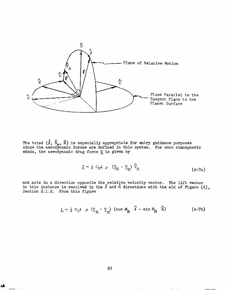
r\ n

AA H

R N

yc

Plane of Relative Motion

Plane Parallel to the Tangent Plane to the Planet Surface

The triad (i, 6,, ?I) is especially appropriate for entry guidance purposes since the aerodynamic forces are defined in this system. For zero atmospheric winds, the aerodynamic drag force D_ is given by

(A-7a)

and acts in a direction opposite the-relative velocity vector. The lift vector in this instance is resolved in the 1 and n directions with the aid of Figure (2), Section 2.1.2. From this figure

4 = 2 Cr,A p (1; xR) (COS #Jo 2 - sin +B 2) (A-7b)

91

Thus, the total aerodynamic force Vector gmRO in the (2, 6,, t) System iS

F = AERO ’

A p ($ l IR) (A-74

where the scalar quantity 5 (V - V ) is the free stream dynamic pressure of the gas flow relative to the vGgiclgrand is denoted by 9. Equation (A-i'c) can also be wri-i$en,in ihe form E vector in the (1 , VR, n) systemyA%!%.

= qC_where C is the aerodynamic control

CLS cos c$

-CDs

-CLS sin% (A-7d)

the components of S may or may not be varied independent of each other depending upon the extent of the vehicle's aerodynamic configuration control.

The triad (fi, fi, k), however , is more convenient for resolving the gravitational forces acting on the vehicle. In this system,the gravitational forceis given by

%RAV = Gmmp $

- (r . r) (A-7e)

where G is the universal gravitational constant and mp is the planet's mass.

* Assuming that all gravitation anomalies can be neglected due to their small magnitudes relative to the other acceleration experienced by the vehicle.

92

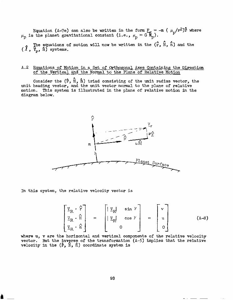
Equation (A-ye) can also be written in the form F = -m ( g/r2)$ where pp is the planet gravitational constant (i.e., pp = G-&p).

(a^ of motion will now be written in the (2, fi, c) and the J

A.2 Equations of Motion in a Set of Ort.nal Axes Containing the Direction of-the

r ..~ ----<- ,C-, - .- -. Vertical and the Normal-to the Plane of Relative Motion -.- --.---- --7..-

Consider the (F, ?I, ?I) triad consisting of the unit radius vector, the unit heading vector, and the unit vector normal to the plane of relative motion. This system is illustrated in the plane of relative motion in the diagram below.

h

In this system, the relative velocity vector is

I = I “RI sin Y

I V-J cos Y

0

V

1 II = u (A-8)

0

where u, v are the horizontal and vertical components of the relative velocity vector. But the invf;rse of the transformation (A-5) implies that the relative velocity in the ($, E, fi) coordinate system is

93

V

= T$90-9) u = II 0

V

u s-in qJ

u cos $

since the transpose of an orthogonal matrix is the same as the inverge. Further, the components of the relative velocity vector+ in the ($, E, fi) system are also given by

(!!iR r cos L $

(!R .G) = dL I- dt

Thus, equation (A-9) can be rewritten in scalar form as follows

dh dt=v

dX = using dt r cosL

(A-9a)

(A-9b)

(A-9c)

(A-9d)

(A-1Oa)

(A-lob)

d& = .u r

(A-lot)

But, the ($, ?I, fi) triad is rotating with respect to the (" 3

, $$, $R) system. Let CU$ denote this relative angular velocity and let the co ponents due to the rotatIona rates be $!,-g, and-g . That is,

* This formulation assumes that the planet is spherical to an acceptable degree of approximation.

94

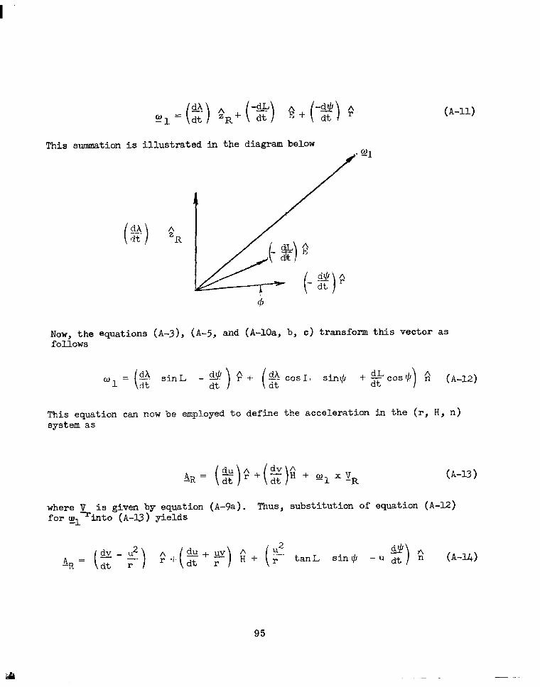
This summation is illustrated in the diagram below

El = (2) GR+ (-g) !$-I- (-g, F

A /

(A-11)

Now, the equations (A-3), (A-5, and (A-lOa, b, c) transform this vector as follows

w1 = dA dt COSIZ Sin+ 2 (A-12)

This equation can now be employed to define the acceleration in the (r, H, n) system as

(A-13)

where V is given by equation (A-9a). Thus, substitution of equation (A-12) for gl rinto (A-13) yields

95

The final step in the derivation of the equations of motion in the (a, $, ^n) system requires that the other inertial acceleration terms in equation (A-2) be evaluated. formations (A-3) and (A-5)

Since u+ = mp !$ then by using the trans-

wp = ( wp sjn L ) r^ + ( up cosL cos + ) 2 + (tip cosL sin 9 ) k (A-15)

The cross product terms in equation (A-2) when expanded become

‘@P x ‘R= 1 -2u (opcosL sin+ ) 9 1 1 A + 2v (up cosL sin+) H

C I (A-16) -I- 2u

( wP sinL)- 2v (WP COSL cos $3) 2

and

x (w_, x2)= (- r w 2

w cos2L ) i! P P

t(r 0 2 P

sinL cos qil cos $b > G

+ (r 0 2 P

Sir-IL cos L sin+ ) 2 (A-17)

Adding the accelerations (A-U+), (A-16), and (A-17) gives the total inertial acceleration of the mass particle. Multiplying this by m, and equating the

to the summation of forces acting- -on the particle-(resolved in-the system) then yields the following scalar equations of motion:

L cos+B cos Y -DsinY -m

sin & ) - r ~~~ cos2L 1 (A-18a)

96

- D COSY - L cos GB SinY

+ 2 v ( op COSL sin+ > + r up2 sinL cosL cos$ I

(A-18b)

-Lsinr$= In ;tanLsin+-y +2u(o/nL)

-2~ (wpcOsL cos+ )+rup2 sinL cosL sin+ 1 (A-18~)

where

L = $ CLS p (u2 + v2>

n = 5 c,sp (u2 + v2)

dh z=V

dA=usimJI dt r COSZ

a= u cos9 dt r

P = P(h)

(A-19)

(A-20)

(A-21)

(A-22)

(A-23 >

(A-24)

97

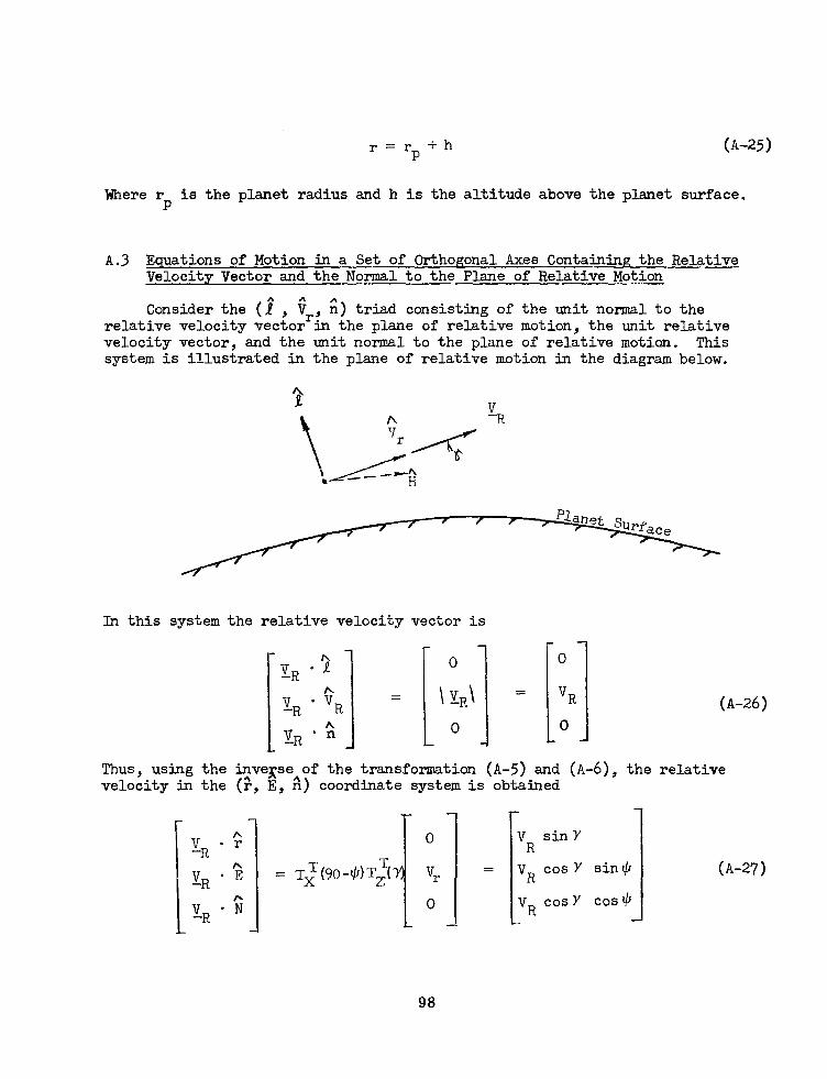
r=rp+h (A-25)

Where rp is the planet radius and h is the altitude above the planet surface.

A.3 Equations of Motion in a Set of Orthogonal Axes Containing the Relative Velocity Vector and the Normal to the Plane of Relative Motion

Consider the (m^ , ?,, G) triad consisting of the unit normalto the relative velocity vectorLm& the plane of relative motion, the unit relative velocity vector, and the unit normalto the plane of relative motion. This system is illustrated in the plane of relative motion in the diagram below.

In this system the relative velocity vector is

Thus, using the invexse of the transformation (A-5) and (A-6), the relative velocity in the (1, E, A) coordinate system is obtained

= TX' (90 - $1 T;t

0

5

0

VR SinY

m I

VR COSY SinqJ

VR COSY COSVJ

(A-27)

98

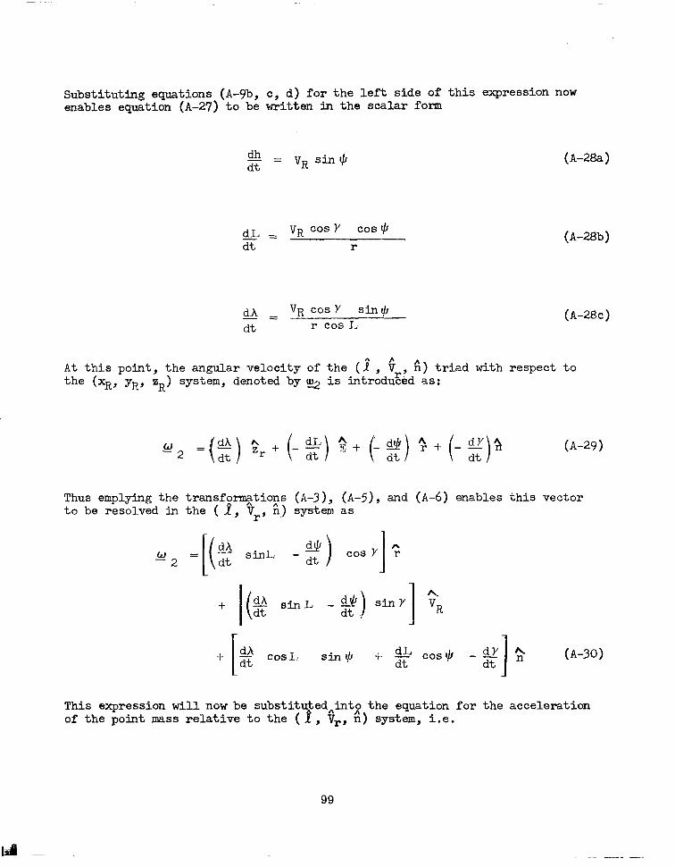
Substituting equations (A-9b, c, d) for the left side of this expression now enables equation (A-27) to be written in the scalar form

g = vRsin+

dL _ vR 'OS' cos $ dt- r

@J _ vR cosy SiIlIjl dt - r cosL

(A-28a)

(A-28b)

(A-28~)

At this point, the angular velocity of the (a", $ , ?I) triad with respect to the (xR, yR, zR) system, denoted by 9 is introd&d as:

(A-29)

Thus emplying the transformations (A-3), (A-5), and (A-6) enables this vector to be resolved in the ( 1, tr, fi) system as

dX J = id! h cosY r

2 2 SinL - dt ) 1 + I( dA dt sinL dlCI SinY VR ’ 1 A

- zi ,

dY 2 -z

I (A-30)

This expression will now be substituted*intz the equation for the acceleration of the point mass relative to the (I, V,, n) system, i.e.

99

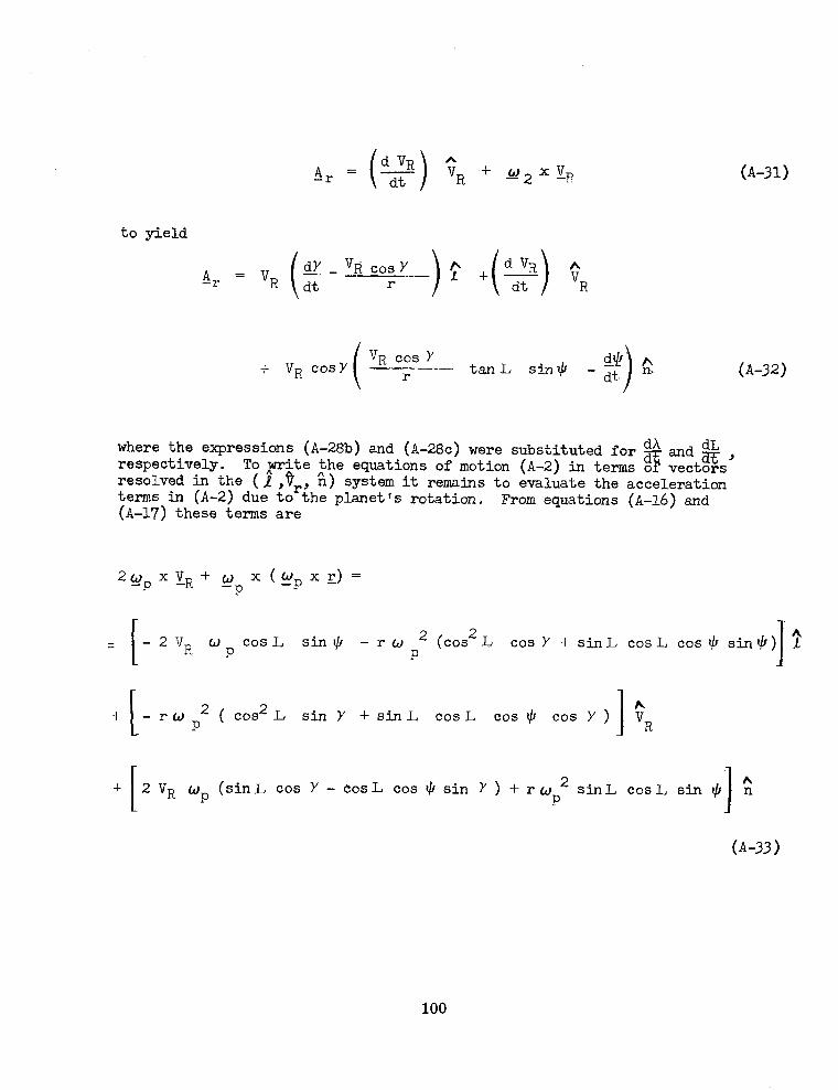
to yield

A = -r %

=

dY -_ - % co9 Y

\ dt r

t VR COSY VR COS Y

r - tanL sin$

A -r + -"22xX? (A-31)

(A-32)

where the expressions (A-28b) and (A-28~) were substituted for dh m,-J dL respectively. To nwrite the equations of motion (A-2) in terms o vect%s' resolved in the (1 ,tr,

di ^n) system it remains to evaluate the acceleration

terms in (A-2) due to the planet's rotation. From equations (A-16) and (A-17) these terms are

2@>oxxR+ k, x (&$,xd= -p

-2VR w cos L -rw cos2L ?

sin $ 2( P

cos Y + Sir-IL COSL cos$ sink) I 2

cos2L sin Y + SinL COSL 1 h t -rw cos $J cos Y > VR

t 2 vR up (sinL cos y - cosL cos3,sin Y)+rg 2 SinL coSL sin $JJ I

h P

n

(A-33 >

100

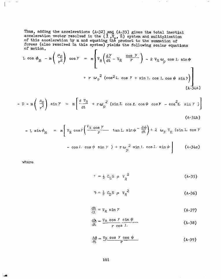
Thus, adding the accelerations (A-32)*ancJ (A-33) gives the total inertial acceleration vector resolved in the (.! ,V,, ^n) system and multiplication of this acceleration by m and equating the product to the summation of forces (also resolved in this system) yields the following scalar equations of motion,

L cos +B - m cos Y -__

r - 2 “p’tdp COSL sin+

+ r UP 2( cos2L cos Y + sinL cos L cos rl/

(sinL cask co.59 cosY - cos2I., sin Y )

(A-34b)

V R cos y - a! r tanL sin+ dt + 2 up VR (sinL CoS Y

- cosL COS$ siny ) + rw 2 sir-L cosL sin* I

(A-34~) P

where

T = $ CLS p VR2 (A-35)

‘,=$ CDS p VR2

--- ;; = VR sin Y

dX = VR COS Y sjn ti

z --

2‘ cos L

&4 = VR cos y cos $ d-b r

(A-36)

(A-37)

(A-38)

(A-39)

101

P = P (h)

r=r +h r'

(A-40)

102

APpENDu[ B ATMOSPHERIC MODELS

Several standard earth atmosphere models are used in entry performance and guidance studies. Among these are the 1959 ARBC model, the lo62 U. S. Standard Atmosphere, and the 1963 Patrick AFB Reference Atmosphere. These models consist of numerical tabulations of the properties (pressure, density, temperature, mean molecular weight, etc.) as functions of either geopotential or geocentric altitude. However, to obtain approximate closed-form flight path solutions for use in an explicit guidance scheme or to reduce the two equations of motion in the local horizontal and vertical directions to a single differential equation for fast-time integration guidance, some simple mathematical relation between atmospheric density and altitude is necessary. This simplification results because the aerodynamic forces can then be related to altitude at any time thereby facilitating the integration. mfortunately, there is no simple mathematical relation between these two variables which is exact; however, for the major portion of the atmosphere the fact that the variations in atmospheric temperature and molecular weight with altitude are small as compared to the variation in density, enables a simple approx5mate density-altitude relation to be derived with more than sufficient accuracy for the purpose it serves. This derivation can be accomplished by examination of the distribution of molecular energy in the gas, or from considerations of static equilibrium of the gas as a continuum. The latter approach is chosen here.

Consider an infinitesimal vertical column of gas having mass m, in static equilibrium, where the horizontal surface area of the coluun~ is A; the volume, dV; and height, dh. The gravitational force acting on the column in the vertical direction is given by -mg, where g is the local value of gravitational acceleration. The pressure differential between the bottom and top of the column is given by dp and the pressure force in the vertical direction by -Adp. To be in static equilibrium, the sum of these forces must be zero, thus Adp = -mg. Now, if p denotes the mean density of the gas in the column, the equation of equilibrium can be written in the form dp = p g dh (m = p Adh). In order to help integrate this the differential form of the equation of state must be used. by taking the logarithm of both sides and differentiating, the form o is:

92 P

=dg+!pg P M

103

where T is the absolute gas temperature, M, the gas mean molecular weight, and R, the universal gas constant. By neglecting the variations in gas temperature and mean molecular weight in comparison to in density, the differential equation of state becomes dp = . Thus, substituting this expression for dp in the static using the original form of the equation of state for a gas yields

LAgdh P

in this differential form is constant, since the temperature and variations with altitude are neglected. Therefore, this

equation can be integrated, with the result being the desired relation between density and altitude, i.e.

In this equation the density value at the planet surface is denoted by p. , and p = gfi/RT. Another form of the density-altitude equation often used is

P = PO exp (- Ph) B-2a

The notation exp followed by a quantity in parentheses means e ( ) , where e is the base of natural logarithms. The inverse relation of B-2a from B-l is

B-2b

The term l/p is called ty atmospheric scale height and is the altitude at Denoting this altitude by the

h = hS In ,$ ( 1 B-2c

104

The validity of this simple mathematical relation for the earth's atmosphere is shown in Reference 1. In addition to the deviation in density from this model due to changes in the gas temperature and molecular weight, there are seasonal, daily, and latitude variations of density. The extent of these variations are discussed in many papers (e.g., Reference 2 and 3). These variations and uncertainties in atmospheric density are dominant factors in the adoption of a closed-loop approach to atmospheric flight guidance.

105

APPENDIX c

APPROXIMATK INTEGRALS OF THE MOTION

FOR VARIOUS FLIGHT MODES

C.l The Equilibrium Glide Solutions

l3y far the most useful of the closed form flight path solutions available for entry guidance is the equilibrium glide solution. Not only is this solution useful for performance prediction, but it is also important as a nominaltra-

jactory for linear perturbation guidance approach (see Reference 9) as a terminating condition for other flight paths, and as an indication of the flight envelope control limit. An understanding of the equilibrium glide also provides more insight into the dynamics of atmospheric entry than any other solution. The phrase ~~equilibrium glide 11 is derived from the fact that the tra'ectory is the solution for which the centrifugal acceleration component

:! (-V /r) of the vehicle balances the resultant acceleration of the vertical* forces acting on the vehicle, i.e.,

- v2 L -=-& cos$ -g r P

C-l

where g P = p/r. pP

In a sense, this path is an extension of the Keplerian flight solution where the aerodynamic lift force is used to counterbalance the centrifugal and gravitational accelerations at velocities other than circular orbit velocity. For velocities less than circular, positive lift must be applied (cos &>O); for velocities greater than circular, negative lift must be used (cos$~<O) for this solution. For atmospheric flight at circular velocity, zero lift is required to fly an equilibrium glide (cos+- = 0). Thus, if fixed aerodynamic coefficients are assumed during the gli -2 e, a family of equilibrium trajectories with bank angle as a parameter is established and equation (C-l) can be written in terms of a dynamic pressure-velocity relation, as

* In the diagram of Figure 2, the 1 direction.

107

‘- --- , ‘I,/. .,.“.’ : .:

m gP S= (1 - i2)

(CL s cm $)E

Solving for the density, yields

P = 2m 1 1 - T-v2 -

(CLS co.5 $)E rP -t2

Thus, the altitude, from the exponential atmospheric model (1.7~) is

(CL s cos QE h = hS In 2m

c-2

c-3

C-L

It can be shown from analysis of the altitude-velocity relation (C-4), that as velocity decreases, the glide altitude increases for v > 1, and decreases for v<l, assuming a fixed value for the term (C S cos 4 ). Also, as the velocity approaches the circular value from either dir ii ? ction, he glide altitude approaches a theoretically infinite value.

This altitude-velocity relation is illustrated in Figure C-l for several values of the vertical lift parameter (CL S cos 4 ). The region to the right of the circular velocity line requires negative 1 4 ft to maintain l'equilibrium," the region to the left, positive lift. The maximum altitude equilibrium glide lines are the lines for maximum CL S in both regions, where in the subcircular velocity realm cos 4

* 3 = 1, and in the supercircular, cos 4B = -1. The regions

above these lines XI xate the flight regime where the dynamic pressure is insufficient for the vehicle to maintain an equilibrium glide condition regardless of the aerodynamic lift commanded.

In the supercircular velocity realm this region corresponds to positive flight path angular rates; in the subcircular realm, negative flight path angular rates. Thus, this is the region where insufficient lift exists to maintain constant altitude flight, or for that matter, flight at any constant or slowly-varying flight path angle. The maximum altitude equilibrium glide solutions, therefore, provide a good indication of the limits of control for the vehicle, and a convenient terminating condition for the remainder of the closed form flight path solutions yet to be developed.'

108

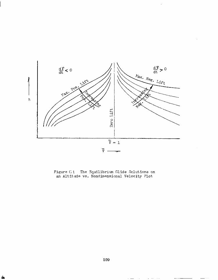
V=l

V---T

Figure C1 The Equilibrium Glide Solutions on an Altitude vs. Nondimensional Velocity Plot

109

Figure C2 illustrates these closed form solutions eminating from a point within.the flight envelope, and terminating on the maximum lift subcircular glide line. A supercircular glide Line could have been used instead, if climbing flight paths in the supercircular realm are desired. In either case, the maximum lift lines are used to indicate the limits of the controllable flight regime. For guidance applications which require increased fletibility in the choice of the final objectives any one of the family of equilibrium glide trajectories can be used as a segment of the flight path.

Some performance prediction equations useful for determining the termLna1 point of the solutions mentioned are now considered. From (C-2) the acceleration along the velocity axes for the equilibrium glide is

2 = - (0 :osJE gp (1 -F2>

(c-5)

and the aerodynamic and (2.1.15) .

load factor and heat transfer rate are from (C-2), (2.1.8),

G= cR

( > CL cos +B E (1 - t2) c-6

a= cH 3/2 dt (CL cos QE mgP

r 2 P (5 - TJ) c-7

The predicted altitude rate, h, is determined with the aid of the chain.rule for derivatives, i.e.,

C-8

110

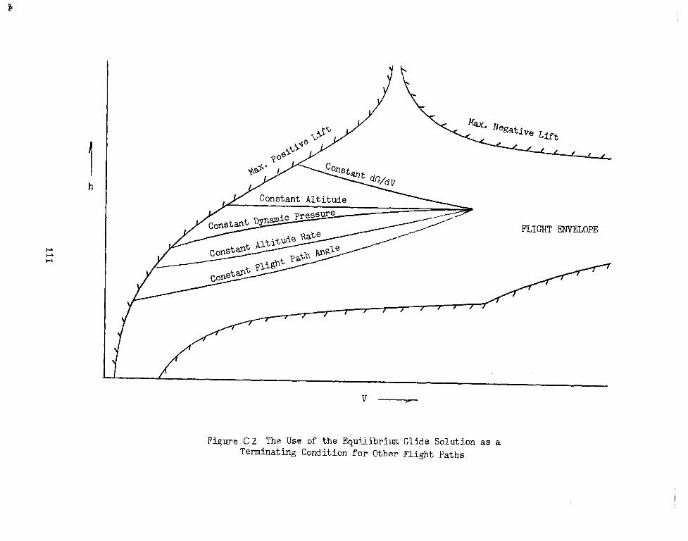
FLIGHT ENVELOPE

v-

Figwe C?. The Use of the Equjlibrilm Glide Solution as a Terminating Condition for Other Flight Paths

Substituting the exponential atmosphere yields

iig= dh - P P

Thus employing the definition

d$ = ti g d?

-4m =

(CL s CfJS 4JB)E

1 L

gp2 'P 3/2

c-9

c-10

and substituting into equation (C-8) yields the relation between altitude rate and velocity as

Thus, the predicted flight path angle (sin Y = h/V) satisfies

siny = -2 hS 1

( rP

c-11

c-12

Finally, the surface arc range traversed along an equilibrium glide line is obtained as follows:

First v R- y df_

dV ” Y

112

Now substituting for g from equation (C-5) and integrating yields

cos cj l-vi2

BE rp In l- it2

c-13

where the subscripts "i" and .?,I' indicate the initial and terminating‘values, respectively. Equation (C-13) is a prediction of the surface-arc range traversed by a vehicle having an effective & value in the vertical plane by given by (6 cos +B)E along an equilibrium g$!ide path for the velocity range between Vi and Vt.

C.2 The Linear Variation of Aerowamic Load Factor,_with Velocity Solution

The second integrable flight path to be considered for performance prediction is the solution for which the rate of change of aerodynamic load factor with velocity is constant, i.e.,

dG dV= constant c-14

A special case of this solution occurs when this constant is zero. In this instance the solution reduces to a constant aerodynamic load factor flight path. Because of the wide application of this constant G solution, the prediction equations for constant G are also given, following the more general solution. If the load factor and velocity at the start of this flight phase are denoted by the symbols G. and V.. Integration of (C-14) relates a linear variation of aerodynamiciload f&.&or to velocity as

dG G - Gi = dv (V f Vi)

or

dG

=G ., constant G 1

113

C-15a

C-15b

Once again, constant aerodynamic force coefficients are assumed; thus, the dynamic pressure variation with velocity is also linear, since from (C-15a)

9 = G (Gi - g Vi> +( 2) s V C-16a

constant G C-16b

Similarly, the drag acceleration is

dV dt = -gp 5 (Gi 'D ~ V

cR CR

= cD G -"p< i, constant G

And the atmospheric density as a function of velocity from (C-16a) is

P G. _ = 1

= - constant G 9

Also the altitude-velocity relation from (B-2c) and (C-18b) is

(G dG ;;+(g)v] i - dV

= h, ln[("" zrnc ) g] ,constantG

114

C-17a

c-17b

C-18a

C-18b

C-19a

C-19b

lb the same manner, the predicted aerodynamic heat transfer rate from (2.1.8) and (C-16a) is ,

dH = Ing dG Ci20a dt

'H PG

(G i

_ '6 dV V2

= mg CH r GiV p R

constant G >

Since the altitude rate can be written using the chain rule for derivatives as

dh dh 3 dt=dV dt

where by differentiating the altitude-velocity expression (C-loa) with respect to velocity,

c-21

G

Substituting (C-21) and the drag-acceleration expression (C-18a) into the altitude rate expression then yields

=- gp hs cD 2G - ii CR ( G-- )

115

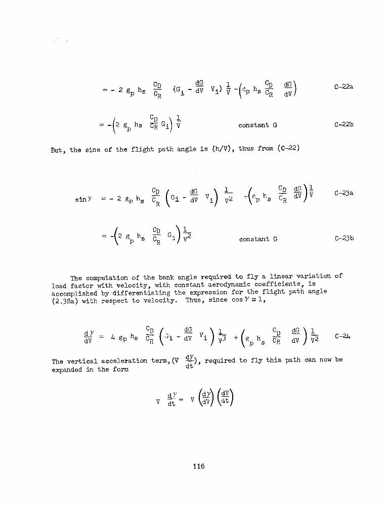
dG = - 2 gp h, ~ (Gi -dV Vi) $-

cD dG 'P hs G dv

CD 1 =- 2 gp hS cfiGj, V constant G

But, the sine of the flight path angle is (h/V), thus from (C-22)

C-22a

C-22b

CD dG ShY =-2gphs C Gi- ii *i

C-23a

R

=- ( 1

2 gp hs 9G cR

i 7 ) constant G C-23b

The computation of the bank angle required to fly a linear variation of load factor with velocity, with constant aerodynamic coefficients, is accomplished by-differentiating the expression for the flight path angle (2.38a) with respect to velocity. Thus, since cosY=l,

dY CD dV = 4 gp hs s h C-24

The vertical acceleration term,(V dY ii& required to fly this path can now be

expanded in the form

116

I

Thus, substituting (C-24) for dY

vertical acceleration term as s and (C-17a) for 2 yields the flight path

=- gt h,($J[L(Gi-$ vi) $? '(%) $lG C-25

Next, substituting the expression (C-25) for V 2 into the equation of motion (2.2.2) and solving for the cosine of the bank &gle yields:

cosc$ = gp(l-&J +4-r

R -- .._...-___ 4. ( ) m

c;L g gp G C-26a

CR (44 .- = cc ----_- ,.

dG dG r,.,- v +- 1 dV i dV ' - gp ‘S( zfX:f) [& (Gi - $)$ +(9 $1

= CL 5 (l - $)-b gp hs 2 z: '$ $ ; constant G

C-26b

117

The terminating condition can be determined from a limiting value of the bank angle or, as will be done here, the intersection of the flight path with an equilibrium glide line*. In most cases, the bank angle limit is the more complex solution. This fact can be shown by solving for velocity in (c-26a) when cos +B is given a fixed limiting value. The general solution is determined in this case by finding the roots of a fifth order polynomdnal. Terminating on an equilibrium glide line, however, has two advantages: first, the glide line may be used as the next flight phase, and second, the solution for the terminating velocity, in most cases, is no more complicated than solving a quadratic equation, Since the altitudes and velocities must be identical at the point of intersection of the two flight paths, the terminating conditions may be determined by equating the altitude-velocity relations for these paths. At the intersection of the constant dG/dV and the equilibrium glide paths, the expressions (C-4) and (C-19a) must have identical values, thus,

Thus, arranging the terms in standard quadratic form yields cos$J ‘i2 + _I_ __-._ cI_ -.-w-E G R i

C-27

bow, the terminating velocity r:tio is one of the roots of a quadratic equation, i.e., Vt = -(b/2) + $ (b2 - 4c)2, where

(CL s cos dJB )E -___, .__ - VC

b= 'Rs

('Ls "'$)E -._._ _ I _ _ -

c= %

Since the terminating velocity ratio Vt is always positive, only real roots are acceptable. Thus, b2> 4c, othemse, the flight paths do not intersect,

*In most cases a subcircular glide line.

118

For the special case where dG/dV = 0, the solution for the terminating velocjtg ratio from (C-27) yields

1 1

(CL S cos B)R 2

CR A Gi * Constant G

Finally, the surface arc range traversed is calculated by the expression (2.32a) for dV/dt into the surface arc integral integrating, that is,

C-28

substituting (2.154, and

V t

Vt V dV V dlJ

-- = 2 1 R= -CD gp

--- dG

'i 'i Gi - iii 'i

C-29a

'i

"t

v- aln (a+V 3

!cfo ; for dV

vi

where

1 dG

a= z ( 1

Gi - z Vi )

dV Substituting the limits Vi, Vt into the integrated range expression gives

C-29b

119

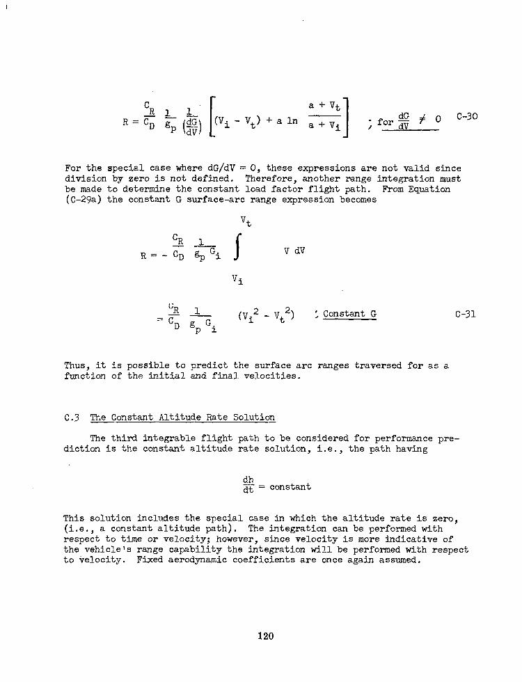
a + Vt

Vt> + a In a + Vi 1 m for E # O c-30 / dV

For the special case where dG/dV = 0, these expressions are not valid since division by zero is not defined. Therefore, another range integration must be made to determine the constant load factor flight path. From Equation (C-29a) the constant G surface-arc range expression becomes

‘R 1 R=-

CR 1 =s g tvi2

pi

V dV

- vt2) ', Constant G c-31

Thus, it is possible to predict the surface arc ranges traversed for as a function of the initial and final velocities.

C.3 The Constant Altitude Rate Solution

The third integrable flight path to be considered for performance prediction is the constant altitude rate solution, i.e., the path having

dh z< = constant

This solution includes the special case in which the altitude rate is zero, ( i.e., a constant altitude path). The integration can be performed with respect to time or velocity; however, since velocity is more indicative of the vehicle's range capability the integration will be performed with respect to velocity. Fixed aerodynamic coefficients are once again assumed.

120

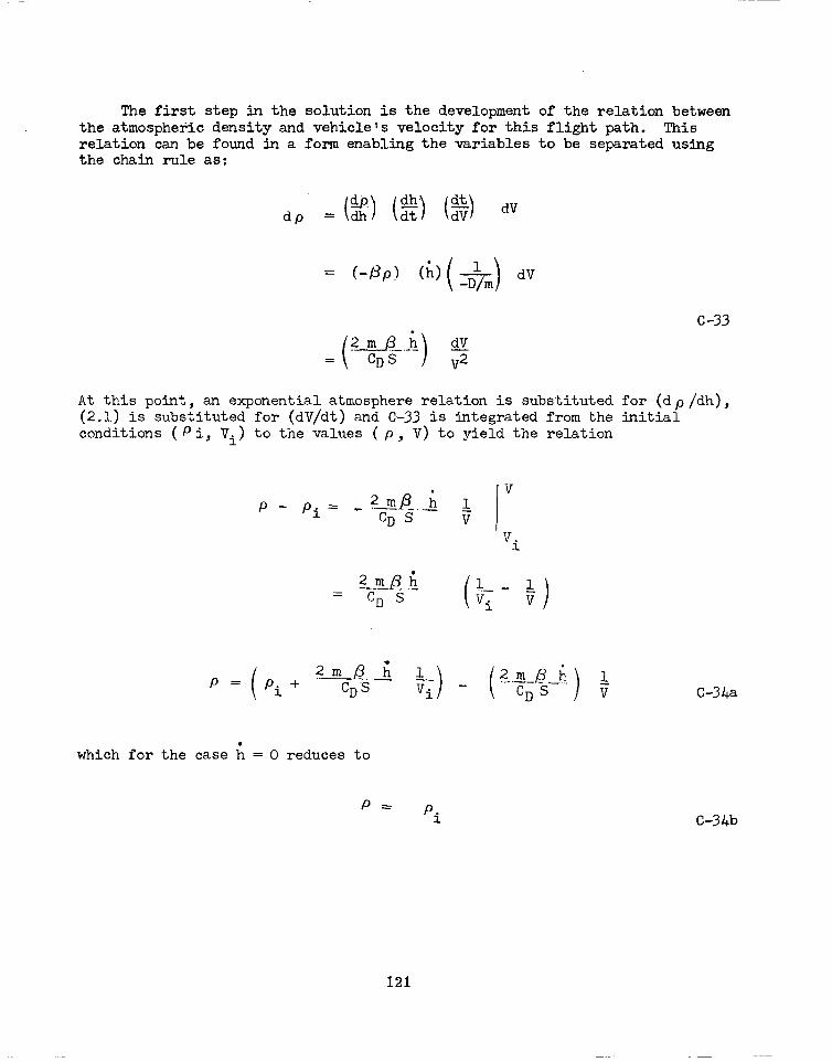
The first step in the solution is the development of the relation between the atmospheric density and vehicle's velocity for this flight path. This relation can be found in a form enabling the variables to be separated using the chain rule as:

dp. = (g) ($, ($ dV

c-33

At this point, an exponential atmosphere relation is substituted for (dp/dh), (2.1) is substituted for (dV/dt) and C-33 is integrated from the initial conditions (Pi, Vi) to the values ( p, V) to yield the relation

P - 2mBi 1 V

pi = - ..c s- D V I

V i

P= pi+ ( 2mfl1; ..- _ CDS

which for the case i = 0 reduces to

P I 'i

c-34.a

C-34b

121

Since the initial density, p., cannot be measured directly, a relation between it and the initial load fact&r can be used to write the prediction equations. in terms of the initial conditions (Gi, Vi). Thus, solving the equation for G for pi yields

p i = z !!I.-

C$ gP ‘%

Thus, the density expressions (C-34) may be rewritten as

c-34c

P = Gi VqT- +

C-34d

or

= 2 m gP Gi

cRs Vi2 Y C-34e

Thus, the dynamic pressure for constant altitude rate can be obtained as

= mgp- Gi v2 ( :F. s “iz )

the drag acceleration,

122

dV = E c-36a

'D Gi V2 ; h=o. c-36b

=- cp & vi--‘

the aerodynamic load factor as

G= 'R ,i)v G

C-37a

P \r. = --.

( ) VI v2 C-37b

and heat transfer rate as CH Gi + 3.

P G Q CD c-38a

= gp v3 .

9

, h=O

The altitude-velocity relation for constant altitude rate can now be obtained as from (C-34d) and (B-k)

h = h, In

C-38b

( 1 CRS

5-c PO V c-39a

-- --.. ---

.( Gi - + 2 -p )v -(Z P

'P Vi2 i q

I

123

h = h- 1 i=o f C-39b

Similarly, since the sine of the flight path angle is simply sin? = h/V, the flight path angular rate is found to be

CD Gi g, CF) VT2 +

CD G- = =P qi$ i + $-g - (p h2) i ., j

where cosY =l and where Equation (C-36a) was substituted for dV/dt. 1, .:

These equations can now be used to develop the control low for the descent. First, the cosine of the bank angle required to fly the constant ' altitude rate flight path is found by substituting (C-39~) into (C-25a), i.e.-.'-'

,+@ v i 1 - h2>

cos 4 = B

V2 - 2 s h + /3 rp $) V +(firph2 - Vg) ( i

_._ -.----- ._A____.___ ____

- ( 'L Gi

, 5 v, Pa! 9 CL vg

"-A iy'$ ) ( CD I B h 1 v c-39d vi -

--.-.- ---_ ..-_.

124

where (L/m) = (CL/C$gpG, and (C-37a) is substituted for G. Thus, the bank angle scheduling for constant altitude rate is seen to be the quotient of two velocity polynomials. Next, the terminating velocity for the constant altitude rate solution is found by its intersection with an equilibrium glide line. At this point, the altitude-velocity relations (C-4) and (C-39a) must be identical in values, i.e.,

62 cRS --

2m P, v -----

2m P, rp y-:3p = ----____

Thus, rewriting this equation in the standard quadratic form allows the following equation to be prepared

@I, s ‘OS +, )E -_-___-.-- ..- Gi ‘R fli 1.+ cR s r? ‘p ~~ + ‘3 lJi )I 62

c-40 (CJJ s cOs 4~ >p -A!

CD l=O

Now, the terminating velocity ratio yt is a root of (C-40), i.e.,

vt = - b +_ (b2 - 4 a c)k

2a

where

(CL s cos+& Gi CR

-- ip

CR @i + G f--

i 13 (CLS cos h )E & p

CD C rP I

125

For the case where b2,<4ac, the flight Paths cannot intersect and no solution exists. The terminal velocity ratio for the constant altitude flight path is shown from (C-40) to satisfy the identity,

i P

1 VP ---

vt = (q-p5 cos $ >T -Gj 1+ -- --__w -- -.._ Yi .._ '.:--

'R ' Vi2 1 constant altitude c-41

Finally, the surface arc range traversed along the constant altitude rate flight path is calculated by substituting the expression (C-36a) for dV/dt into the surface arc integral and integrating

VdV - --_-

vi (g-l) v - (gp : + + ff) v2

where

i

dV

A -BV

lTt

1 =- B In (A-BV) = i ln(A-BV)

n B

"D Gi = gP GR ~ +

'i

C-42

126

Thus, substitution of the limits into the expression C-42 yields the surface arc range as

CD Gi

gP < i$

1 'R 'i2 In (5) =5 5g- Vt

In

[ (

cR _- CD 2 fj)[z - ') + z C-f+Ja

A 1 ( 1 il =o

Equations (C-43) estimate the surface arc range traversed by the vehicle a constant attitude rate flight path from initial velocity, Vi, to final velocity Vt.

C-43b

along

C.4 The Constant Flight Path Angle Solution

The fourth integrable flight path to be developed for performance prediction is the constant flight path angle solution, i.e., the path having

Y = constant C-44

The first step, as before, is the development of the relation between the differential density change (dp) and a differential velocity change (dV) by employing the chain rule

do =(%)(%)(%j dv

= (-&) (V siny) (-6-f-p) dV

c-45

Gi-.kL~- m sin Y 1 = 'D s V

127

But this differential equation can be integrated from the initial conditions V) to yield the constant Y flight path density-

2pl_m_-s~ Y -- P - oi.= 'D s

2 /3 m sin Y V -- --..__- _ _ In P = Pi + cD ( 1 q

C-46a

C-46b

But, the density is not a direct measurement, thus, the initial density is given as a function of the initial load factor from Equation (C-24~) as

P =

This equation can now be employed to yield the predicted dynamic pressure for this flight phase as

; = ZL Gi

cR Q v2 +

pm SinY -w _-__^. cD s

The drag acceleration, (from (2.28)) as

'Ds dV- - - -- s dt m

CD Gi v =- ( G gP 7 )

v2 - ( p sin Y > V2 IJJ 7 ( 1

i i

c-47

C-48

c-49

128

The aerodynamic load factor, and heat transfer rate equations (2.2.8) as

z=c,s qv

c-50

c-51

msiny

and the altitude-velocity relation from B-2c as

w

cRs .-- 2.m gp

-- ___~_ -_ -_.--. -_

1 C-52

At this point, the control required can be found. First, the cosine of the bank angle is obtained from (2.2.2) as

cos ~B = [“p y?] = [ gf.q

c-53

[

13 = .--

($ vj) 72 +($ z siY)S2 h(z) 1 129

Next, it is noted that the terminating velocity for the constant flight path angle solution is determined by the intersection of this path with an equilibrium glide line. This intersection in turn is obtained by matching the altitude- velocity relations (C-4) and (C-52). That is,

[ EL s --cos2B _. )E $2 ( ri ---. = 2;;; -- PO rp 1 -i2

[

CR S Gi --- 2m gp q po

--. -_-- _ _ ----.- --... .-_. - -_-

1+- ( cR CD

.@ SaLY- In v_

,gP 1 Vi

In contrast to previous solutions, an explicit solution for the terminal velocity is not possible. Therefore, an iterative procedure must be used. This iteration is facilitated, however, if the equation is rearranged in the form

Vi2

vt = -I[ -4

cR 1+ - . B.~&e-. In Et. + 1

'i cD gP (‘I ) 'i c-54

This form of the solution is referred to as the method of false position. A first guess of V is made by assuming sin?' = 0 and solving for Vt; then the iteration continkes until convergence occurs.

Finally, the surface arc range traversed along the constant flight path angle solution is calculated by substituting the expression (C-49) for dV/dt into the surface arc integral and integrating. This result is

R= a VdV Gi --

---_--

'i gP vz ) IT2 + ( 6 sin Y ) V2 In

i

'i = d V -- __ -__ V a +b In

Vt

130

where

' In 1 vi v

R= b a +b In 5

vt

( CD Gi a= c- R gP q 1

c-55

Substituion of the limits into (C-55) yields the predicted surface arc range as a function of the initial and final velocities, i.e.,

R= hS 1 ----- In -.----- - ..-- --____-- sin Y

1+ "R -kissin y - -_ Vi2 c-56 C D

Zp I+

where h S

=1/p.

131

C.5 The Constant Velocity Transition Solution

In each of the closed form flight path solutions a relationship exists between the variables of altitude, flight path angle, and velocity. However, in general, the existing flight conditions will satisfy the closed form relations for the desired path; as a consequence, the vehicle will not instantaneously follow the desired path. Thus, a maneuver must be performed prior to the time that the desired flight path is attained. That is, another trajectory which starts at the existing point, (h, V, 2 ) and terminates at a desired set of conditions (h, V,$ must be commanded.

I? Unfortunately, an

exact solution of the equations of mo ion which satisfies this two point boundary value problem cannot be obtained; thus, it is necessary to make an assumption which will allow the development of an analytic transition path. This assumption is that the velocity of the vehicle is constant during the transition maneuver.

Although no unpowered entry vehicle can satisfy this condition, the integration performed with this assumption can predict the variation of altitude rate as a function of altitude with sufficient accuracy to control the vehicle. A comparison between this solution and the exact solution as integrated on an analog computer is made in Reference 10. Since velocity is assumed constant only the vertical lift acceleration equation (2.2.2) will,,be integrated. Further, the aerodynamic control vector component in the 1 direction (i.e., CL S cos$ ) is assumed to be fixed during the maneuver. With these assumptions, the common set of assumptions previously adopted, the vertical acceleration equation can be integrated in closed form.

Equations (A - 18a) and (A - 34.a) indppendix A show that for small flight path angles the acceleration term V dt the vertical acceleration d2h/dt2.

is approximately the same value as Thus, the equations of motion (2.2.2)

will be transformed using the chain rule, as

With this substitution, the equation motion (2.2.2) can be written in a form suitable for integration as

b L “$=m

v2 cos c$ B -g+ ;- c-57

Multiply both sides of C-7 by the diff$rential altitude dh and substituting the expression CL S p. exp (- P h) V for L then yields

2

132

hdh = CL s -. ‘OS 4B V2 .-_- -

2m P, V2 exp (-p h) - g + ;'- 1 dh C-58

where the subscripts 1 and 2 denote the constant velocity transition 'maneuver. CL s cos qR are assumed constant, C-58

h2

initial and final values of Now, since velocity and the can be integrated to give

c2 -- 2 PO

V2 exp (-p h)

'hl

the factor

h2

hl c-59

when the constant CL S cos gB has been subscripted to denote the transition path. Substituting the limits into the expression (C-9) and rewriting then gives a solution relating altitude rate with attitude for the maneuver, i.e.,

.2 .2 hl h2

- -- 2 =

[

h, (CL s cos 4B )TR,ANS h2 --.,

___-... .-. .- PO v2 2 2m I[

exp ( - -

hS 1

-

c-60

=P(-?)] + (v”, (h2-hl) where the scale altitude c-60 relates the initial final altitudes (hl, h2) CCL ' 'OS $ )ms.

symbol h , has been substituted for (l/p). Equation and fina 7 attitude rate (hl, h2) to the initial and for a constant velocity maneuver with fixed control

This relation can be used to control the vehicle by adjusting the velue of (CL S cos gB ) from an existing point (hl, V, h ) to one of the closed form flight path solutions already developed. Ho&ever, to do this, it is convenient to use (c-60) in another form,

133

.2 82 hl h

2 (CL s 'OS 'B TP,AN > -. -- -_ - ----- = a-

i- 2 q2

I[

-hs ;q:;) (h%!k, C-6i

where q2 is the dynamic pressure at altitude h2.

If it is assumed that an equilibrium glide is desired, the final values for the altitude, h , and altitude rate, h , should correspond to the corresponding valueg for that velocity uses in the transition maneuver. From (2.19), (2.26) and (2.17) the attitude, altitude rate and dynamic pressure for the equilibrium glide are respectively

h2 = hE = hs In ‘i2

% rp --- (1 - 72)

3. R - -- ( ‘I 1 r

P c

(1 - ?2)

c-62a

C-62b

C-62c

Thus, subsituting the equilibrium glide expression for h and q into c-61 yields the relation between h and h for transition to an equili&ium g&de flight path:

2

- hs

(‘1 ’ ‘OS +B &PANS w2s-..- - ..-- -_ _

134

h l- -d -

- hE ---)

hS II c-63

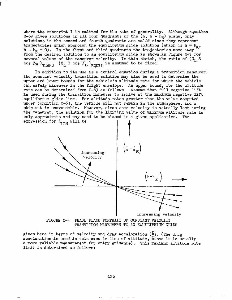
I’ -

where the subscript 1 is omitted for the sake of generality. Although equation C-63 gives solutions in all four quadrants of the (h, h - hE) plane, only solutions in the second and fourth quadrants are valid since they represent trajectories which approach the equilibrium glide solution (which is h = hE, h-

"F = 0). In the first and third quadrants the trajectories move away

from he desired solution to an equilibrium glide is shown in Figure C-3 for several values of the maneuver velocity. In this sketch, the ratio ,of (CL S 'OS @B )TRANS (CL s cos @B )EQ~L is assumed to be fixed.

In addition to its use as a control equation during a transition maneuver, the constant velocity transition solution may also be used to determine the upper and lower bounds for the vehicle's altitude rate for which the vehicle can safely maneuver in the flight envelope. An upper bound, for the altitude rate can be determined from c-63 as follows. Assume that full negative lift is used during the transition maneuver to arrive at the maz&mun negative lift equilibrium glide line. For altitude rates greater than the value computed under condition c-63, the vehicle will not remain in the atmosphere, and a skip-out is unavoidable. However, since some velocity is actually lost during the maneuver, the solution for the limiting value of &mum altitude rate is only approximate and may need to be biased in a given application. The expression for h LIM will be

I t

I increasing velocity FIGURE C-3 PHASE PLANE PORTRAIT OF CONSTANT VELOCITY

TRANSITION MANEUVERS TO AN EWIIJBRIUM GLIDE

given here in terms of velocity and drag acceleration (g). (The drag acceleration is used in this case in lieu of altitude, %!ince it is usually a more reliable measurement for entry guidance). This maximum altitude rate limit is determined as follows:

135

h -- exp (- ‘-hs >

h - hv -.LJ = h3

P b ‘i cos ‘B jMEAS -_.-- -A--.- II

=

-In - In k ': 'OS +&AS

V2 (g - ;;-I .

c-64

The positive root of the expression c-64 is taken for the maximum altitude rate limit.

Similarly if the lower altitude boundaries of the flight envelopes are employed, the lower bound for the altitude rate limit can be determined. This lower altitude bound, for most vehicles, is fixed by either a maximum load factor or a maximum aerodynamic heat transfer rate, depending on the vehicle's heat protection system, velocity, and other factors discussed in the vehicle/ crew limits section. The example given here is for the maximum load factor limit, although the limit for maximum heat transfer rate can be found without additional difficulty.

The transition maneuver required to attain a constant load factor trajectory will be developed and then reduced to the limiting case. From equations c-196, c-226, and C-166 the altitude, altitude rate, and dynamic pressure relations for the constant load factor flight path are

h2 = hG = hs In cRs PO --- -- 2m G )

19

. h2 = l& = -

C 2ghs $ G

C-65a

C-65b

136

C-65c

Thus, substituting the expressions into the constant velocity transition solution C-61 yields the constant load factor transition solution,

-hs(g-;) (7) C-66

the minimum value of altitude rate is now defined by using

G=r, =- m2x

'R !, (2) CD g m max

exp (-

as substitutions into (C-66).

The result is:

i-l 2 2

LTM -- = 2 c 1 hs (:,

F”L4X

C-67

137

The negative root of h calculated from the expression (c-67) is the lower bound to be used. LIM'

c.6 The Ekoatmospheric Solution W-F

The final closed form solution with application to entry guidance is the exoatmospheric or Keplerian conic solution* developed in Reference 11. For this case, the ballistic range expression and ballistic range sensitivities to the exit conditions are given as a function of etit velocity and flight path angle. Further, the conic motion integral yields the radial distance as a functi.on of the semi-latus rectum, eccentricity and true anomaly as

r= .--._ P --.._. _. 1 + e cos 8 c-68

The ballistic range angle 2f3' (see Figure C-4) is equal to twice the difference between 180" and the true anomaly, 8 Solving (2.83) for the range angle then gives EXIT)

c-69

But, the semi-latus rectum is given by p = h2/p thus, the ratio p/rEXIT can be written in the fog,

where h = (r V COSY)~~~;

EL -- = (r V2 ~PGY)~~T

- %XIT --

f-$3 -

c-70

= (i2 cos2 Y )?nT

* The 2-body solution has application only to those entry concepts employing a controlled atmospheric exit. Thus, this concept is predicated on the assumption that this type of operation is both feasible and satisfactory from the standpoint of the mission.

138

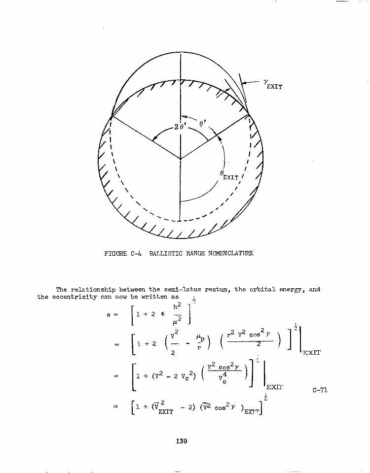
Y EXIT

FIGURE C-4 BATJLISTIC RANGE NOMENCLATURE

The relationship between the semi-latus rectum, the orbital energy, and the eccentricity can now be written as j

h? z

e= I- + 2 d -2 II 1

r2 v2 cos2 Y 2

= 2 EXIT _1 2

=

[

v2 cos2y 1 + (v2 - 2 vc2) ( V,” ‘I EXIT CY71

= 1+(Y2 EXIT - 2) (9 cos2Y lEXTT 1

1 ‘L

139

where E denotes the energy per unit mass given by (V2/2 - c',/rp). Now, substituting (c-70) and (c-71) into the ballistic range expression (C-69) yields

f

(1 -F cos2 Y )EXTT

28' = 2 cos -1 -.

C 1 + (? - 2) (72 cos2Y

1 )I’,, -I c-72

The sensitivity of this range angle to errors in exit velocity and flight path angle are derived by forming the-partial derivatives as follows:

r 3 .,-!a(2 =

dVE)CTT 2kl cos2 y

EXIT I l-c-

k2 (1 - VFXITG) --I--

e L 1 2

9 ( 2 - 1+ Ti”YTT 2, > -- e

where

2 T&-vi- kl = 2$

e (1 - k2 )

C-73a

I C-73b

C-7&

C-74b

and (C-70), (C-71) give (A and llell, as functions of the exit velocity and flight path angle.

140 NASA-Langley, 1968 - 30 CR-1013

GUIDANCE, FLIGHT MECHANICS AND TRAJECTORY OPTIMIZATION

Documents

Transcript of GUIDANCE, FLIGHT MECHANICS AND TRAJECTORY OPTIMIZATION