Submitted: February 2006 Revised: November 2006

Second revision: December 2006

Growth, Population and Industrialization and Urban Land Expansion of China1

Xiangzheng Deng, Jikun Huang, Scott Rozelle and Emi Uchida*

* Xiangzheng Deng is senior research fellow of the Center for Chinese Agricultural Policy, Institute of Geographical Sciences and Natural Resources Research, Chinese Academy of Sciences, Beijing 100101, China. Email address: dengxz.ccap@igsnrr.ac.cn. Jikun Huang is professor and director of the Center for Chinese Agricultural Policy, Institute of Geographical Sciences and Natural Resources Research Chinese Academy of Sciences, Beijing 100101, China. Email address: jkhuang.ccap@igsnrr.ac.cn. Scott Rozelle is the Helen F. Farnsworth Senior Fellow in the Freeman Spogli Institute for International Studies, Stanford University, Encina Hall East, E301 Stanford, CA 94305-6055, USA. Email address: rozelle@stanford.edu Emi Uchida is Research Assistant Professor of Department of Environmental and Natural Resource Economics, University of Rhode Island, Kingston, Rhode Island 02881, USA. Email address: emi@uri.edu

1 Corresponding author : Xiangzheng D eng, Tel: 86-10-64888980; Fax: 86 -10-64856533; Email: dengxz.cc ap@igsnrr.ac.cn.

Growth, Population and Industrialization and

Urban Land Expansion of China

Abstract China is experiencing urbanization at an unprecedented rate over the last two

decades. The overall goal of this paper is to understand the extent of and the factors driving urban expansion in China from the late-1980s to 2000. We use a unique three-period panel data set of high-resolution satellite imagery data and socioeconomic data for entire area of coterminous China. Consistent with a number of the key hypotheses generated by the monocentric model, our results demonstrate the powerful role that the growth of income has played in China’s urban expansion. In some empirical models, the other key variables in the monocentric model—population, the value of agricultural land and transportation costs—also matter. Adapting the basic empirical model to account for the environment in developing countries, we also find that industrialization and the rise of the service sector appear to have affected the growth of the urban core, but their role was relatively small when compared to the direct effects of economic growth. We also make a methodological contribution, demonstrating the potential importance of accounting for unobserved fixed effects.

Keywords: Urbanization, spatial scale, monocentric urban model, industrialization, remote sensing, econometric analyses, decomposition analyses, China

1

Growth, Population and Industrialization and

Urban Land Expansion of China

Economists in urban economics have long been interested in understanding the

process of urbanization. In one of the earliest theoretical efforts, researchers defined

and identified theoretically a number of the causes and consequences of the expansion

of urban land [1, 20, 23]. Among other things, the monocentric urban model generates

hypotheses linking the changes in urban land area to some of the fundamental

building blocks of economies: income, population, agricultural land values and

transportation costs. In subsequent years, empirical economists have tested these

hypotheses with increasingly large data sets and increasingly precise measures. Many

of them—from Brueckner and Fansler [2] to McGrath [18]—find support for the

prediction of the monocentric city model.

Interestingly, although perhaps unsurprisingly, almost all large, systematic

studies of the determinants of urban area have been done in developed countries. This

is in spite of an argument that an understanding of urbanization is even more

important in the developing world since cities are growing faster in developing

countries, problems related to the conversion of land into built-up area are more

severe and the scope for intervening (as well as the potential gains from good policies)

may be greater. That is not to say that there have not been efforts to study the process

of urbanization in developing countries and its causes [10, 27, 29, 30]. But, most

likely due to data limitations, large, nationwide econometric studies using high quality

data are rare.

2

In response, the overall goal of this study is to provide empirical-based

evidence that will help answer several key questions on the extent and causes of urban

land expansions in the developing world—focusing in our case on China. Specifically,

this study will begin with a conceptual framework from the urban economics

literature and test a series of hypotheses from the monocentric city model using a

China-wide dataset on the expansion of urban area in more than 2000 “metropolitan

regions” over time. In the pursuit of this objective, we will seek to answer several

fundamental questions about China: During the reform era, what has been the extent

of urban land expansion of China? What are the main determinants that explain urban

land expansion during the reform era? Which factors have been the most important in

terms of their impact on the expansion of urban land? Taken together, we hope that we

can provide information to policymakers about the extent and main causes of

urbanization in China so that urban land use policy will have a more empirical basis.

More generally, we also will show that when urban economists have access to data

over time the choice of methodology that can control for many of the unobserved

factors which affect the expansion of a region’s urban area will affect the findings.

The rest of this paper is organized as the follows. The next section reviews the

urban economic literature—both theoretical and empirical—and motivates the

hypotheses to be tested. The third and fourth sections introduce the data used in this

study and review the record of urban land expansion across China and how it

correlates with some of the key variables that we are interested in. The fifth and sixth

sections present the empirical model and describe the findings of the two main parts

3

of our analysis: the determinants of urban expansion (in the econometric analysis) and

measurement of the importance of the different determining factors (in the

decomposition analysis). The final section concludes.

Spatial Scale of Cities—Theoretical and Empirical Background

The fundamental theory in urban economics relevant to spatial expansion of

urban areas is the monocentric urban model [1, 20, 23]2 . In the model x denotes

the distance from the central business district (CBD); it is equivalent to the radius of a

circle. Urban residents commute to the CBD, where they earn income y and incur a

commuting cost t per unit of distance. Land rental ( )r and land consumption per

capita ( )q are functions of the distance from CBD ( )x , income( )y , commuting cost

( )t and a common utility level enjoyed by the residents ( )u . Hence, these variables

can be expressed as ( , , , )r x y t u and ( , , , )q x y t u .

The main idea of the monocentric model is that the distance to the edge of the

city ( x% ) and utility adjust until the two following conditions hold:

0

2( , , , )

x x dx nq x y t u

π=∫

%

(1)

( , , , ) ar x y t u r=% (2)

Equation (1) requires that at equilibrium the total population fits inside the urban area.

Equation (2) requires that the urban land rental and agricultural land rental are equal

at the edge of the city. Based on these relationships, the implications of the model can

2 More recent studies have argued that the monocentric urban model is inadequate to explain the more complex, polycentric str ucture of the metropolitan regions in the U.S. (e.g., Fujita and Ogawa [10], Garreau [11], McDonald [12]). Some have argued that the appearance of multiple employmen t centers in the urban area has systematically contributed to expansion of urban area s throughout the post -war period. Others have identified fiscal and social disparities betwee n cities and suburbs as another factor explaining urban expansion . While these factors have been found to be important in the U.S., in this study we first test the monocentric urban model.

4

be seen from the comparative statics. In short, the model implies that:

0, 0, 0, 0a

x x x xn y t r

∂ ∂ ∂ ∂> > < <

∂ ∂ ∂ ∂% % % %

,

or that urban area is increasing in population and income and is decreasing in

transportation costs and agricultural rental rates [33].3

In adapting this model to testing in the developing world (including China),

several factors need to be considered. In many developing countries, it is important to

consider how well land markets operate. It is possible that without well-defined forces

of supply and demand, there could be either excessive spatial growth of cities

(perhaps the most plausible result of poor markets) or excessively limited growth. In

the case of China, for example, prior to the reforms in urban land markets in the

late1980s, land markets in China were nearly non-existent; and land allocation and

development construction were controlled by the state [31]. Since 1988, land use

rights have begun to be commercialized and the land leasing market has begun to

develop. The depth of the reforms, however, varies across regions. While the reforms

have moved forward aggressively in some coastal provinces (Liaoning, Beijing,

Tianjin, Hebei, Shandong, Jiangsu, Shanghai, Zhejiang, Fujian, Guangdong and

Hainan), allocation of land for development by the state still remains the primary

method used to distribute rights to use urban land. It has been estimated that rights

allocation accounts for nearly three-quarters of the transactions and about 70 percent

of land area distributed in the primary urban market during the 1990s [9]. These

3 Although the comparative stat ics shown above are for the distance from CBD to urban fringe ( )x% , the signs

are identical for the total urban area ( 2A xπ= % ), which in this study we use as the dependent variable of the empirical model.

5

observations suggest that there are likely to be factors that determine spatial growth of

cities that are not captured in the monocentric model.4

In addition, the process of development and urbanization overlap in several

other key areas. In the case of all economies that have developed during the 20th

century, one empirical regularity is that as income growth has occurred, the structure

of the economy has shifted from one that is based on agriculture to one that is

increasingly dependent on manufacturing and the rise of service sector. Both of the

expansion of industry and services logically will have an impact on changes to the

size of the urban area. Hence, additional factors should be considered in studies (or at

least controlled for) in study of the determinants of urbanization in China.

Empirical approaches

Two of the most well-known previous studies that have tested the hypotheses

of the monocentric model using data from metropolitan regions in the United States

are by Brueckner and Fansler [2] and McGrath [18]. Brueckner and Fansler [2]

utilized cross-sectional data from 40 small metropolitan regions. In each metropolitan

region, the urban area that was contained within a single, relatively small county was

measured. In their study they found that income, population and agricultural rental

were statistically significant determinants of total urban land area. Each of these had

the sign that was consistent with the prediction of the monocentric model. The

coefficients of the variables measuring transportation costs were not significant.

More recently, McGrath [18] utilized a panel data set for 33 US metropolitan

4 In the monocentric model all factor markets are assumed to be competitive . If the assumption of competitive rental market s does not hold, the equilibrium defined in (2) may not hold. Hence, although we use this to motivate our empirical model , it certainly is not a sufficient model to describe all of the urban expansion in China.

6

statistical areas from the decennial census data from 1950 to 1990. The study used

total urbanized land area in square miles for the 33 cities in each sample area. These

measures were then converted to a variable that proxied for city radius. This study

also found that income, population and agricultural rent were statistically significant

determinants of urban expansion in the U.S. with signs that were also consistent with

the hypotheses. Unlike Brueckner and Fansler [2], however, McGrath [18] found that

the coefficient on the transportation costs variable was also statistically significant and

had the expected (negative) sign.5

Importantly for our study, in addition to the four determinants of urban

expansion that were included in Brueckner and Fansler [2], McGrath [18] also

included a time trend variable to control for the fact that the data came from five

decades in order to capture the time-variant unobservable factors that are common

across all metropolitan areas. The study found that even when income, population,

agricultural rents and transportations costs were held constant, the decade (or time)

dummy variable was significant and the magnitudes and levels of significance of

some of the coefficients changed (in particular, the coefficient on the transportation

variable became negative and significant). However, methodologically the basic

model still relied on the Ordinary Least Squares estimator and did not attempt to fit a

first-differences or a fixed effects model to capture time-invariant unobservable

factors that may bias the coefficient estimates.

5 The two studies used different proxies for transportation cost. Brueckner and Fansler [2] used two vari ables: percentage of commuters using public transit (high percentage implying high transportation cost) and percentage of households owning one or more automobiles (high percentage implying low transportation cost.) McGrath [18] used average annual CPI for private transport ation for each year, rescaled to each region using private transportation cost data for 1990.

7

Using the size of the elasticities as measures of importance, among the four

factors, Brueckner and Fansler [2] found that the most significant determinant of

urban area was income (with an elasticity of 1.50), followed by population (1.10) and

agricultural rent (-0.23). In contrast, McGrath [18] found that the most significant

determinant was population (0.38), followed by income (0.33), transportation cost

(-0.28) and agricultural land value (-0.10). The smaller coefficients found in

McGrath’s study may be partially due to the inclusion of time trend variable.

Data

One of the strengths of our study is the quality of data that we use to estimate

changes in urban land use. For our purposes, satellite remote sensing digital images

are the most suitable data for detecting and monitoring land use change (LUC) at

global and regional scales [13]. Remote sensing techniques also have been used

widely to monitor the conversion of agricultural land to infrastructure [3, 19, 26, 34].

In China land use change has been tracked by remote sensing data [14, 28, 29].

In our study we use a land use database developed by the Chinese Academy of

Sciences (CAS). The data are from satellite remote sensing data provided by the US

Landsat TM/ETM images which have a spatial resolution of 30 by 30 meters [32].

The database includes time-series data for three time periods: a.) the late 1980s,

including Landsat TM scenes from 1987 to 1989 (henceforth, referred to as 1988 data

for brevity); b.) the mid-1990s, including Landsat TM scenes from 1995 and 1996

(henceforth, 1995); and c.) the late 1990s, including Landsat TM scenes from 1999

and 2000 (henceforth, 2000). For each time period we used more than 500 TM scenes

8

to cover the entire country. Specifically, we used 514 scenes in 1988, 520 scenes in

1995 and 512 scenes in 2000.6 A hierarchical classification system of 25 land-cover

classes was applied to the data. In this study the 25 classes of land cover were

aggregated further into six classes of land cover–cultivated land, forestry area,

grassland, water area, built-up area and unused land. The data team also spent

considerable time and effort to validate the interpretation of TM images and

land-cover classifications against extensive field surveys [16].7

Creating Measures of Urbanization

Before creating a measure of the change in the spatial scale of China’s cities,

we need to make several key decisions. First, in this study we use the county as the

analytical unit. The county is the third level in the administrative hierarchy in China

below the province and prefecture. Although we generically use the term county for

all of our observations, our choice of analytical unit includes (autonomous) counties,

county-level cities, banners (which are county-like administrative regions in northern

China) and districts. There are over 2000 counties in China. We use the county as the

analytical unit because in China we believe each county can be regarded as an

administrative as well as an economic region. The average area of a county is between

3000 to 4000 square kilometers. Historically, counties grew up around an urban center,

the county seat. Today, each county hosts an important administrative level of

government (the county government) and in almost all cases one of the functions of

6 A TM scene is the unit of area of coverage of digital images th at are made by Landsat satellites. In the original Landsat material, which was configured by NASA before they provided the material to CAS, it took about 500 scenes to completely cover all of China’s territory. 7 Additional details about the method ology, which we used to generate the databases of land cover from Landsat TM, are documented in Liu et al. [15] and Deng et al. [5].

9

the county government is to create its own land use plan and, as such, constitutes a

region that can be used to study land use changes—especially of the urban core.

Studies that examine changes in urban land using Landsat images also need to

make an important choice regarding the definition of urban land. Specifically, we

need to decide what exact type of built-up area in each county constitutes urban land.

Our data set includes three classifications of built-up area: the urban core, rural

settlements and other built-up area. In constructing our data set, the urban core is

defined as all built-up area that is contiguous to urban settlements. Each county in our

sample, by definition, has at least one urban settlement. In other words, it is possible

to have more than one urban settlement in a county. When there is more than one

urban settlement, the sum of the areas of the urban settlements equals the area of the

urban core. The expansion of the urban core from one time period to another is

defined as all new built-up area that has appeared (e.g., between 1988 and 1995),

which is contiguous to the urban settlements in 1988. The rural settlements category

in our dataset includes all built-up area in small towns and villages. Urban settlements

are differentiated from rural settlements during the interpretation phase of the data

analysis according to standard Landsat imagery. Rural settlements can become urban

settlements in two ways: by being surrounded by new built-up area and becoming part

of the contiguous urban core; and by growing themselves to the point that the Landsat

images change in color, texture and tone. The other built-up area category includes

roads, mines and development zones that are not contiguous with the urban core.

10

In this study we choose to focus on the urban core part of built-up area. In

simplest terms we choose to focus on the urban core for both practical and realistic

reasons.8 First, the data on the urban core is thought to be higher quality (mainly due

to the fact that technically it is easier to identify the urban core compared to other

types of built-up area), which will mean that the dependent variable in the analysis

contains less inherent measurement error. Second, the urban core part of built-up area

in China constitutes by far the type of built-up area that is growing the fastest.

One of the most onerous tasks in preparing the data was to create a set of

county-level analytical units that were consistent over the study period. The problem

of consistency of county-level analytical units over time arises because of changes in

jurisdictional areas in administrative regions. The boundaries of some counties

changed over time. In other cases towns in a single county were divided into two

groups and made into two counties during the 1980s and 1990s. Occasionally the

urban core of a county was removed from the jurisdiction of the original county

government and became an independent county-level administrative unit.

Because of these changes the number of counties rose over the study period.

For example, in 1988 China had 2,156 administrative units at the county level,

whereas in 2000 the number expanded to 2,733. The organizational shifts of

county-level administrative units are problematic for this study since data within each

county observational unit need to be comparable over time.

8 Since we also are interested mainly in the process of urbanizatio n, we do not include area built-up in rural settlements, although this is analyzed in Huang et al. [11]. Finally, unlike many studies in develo ped countries that are interested in urban sprawl (e.g., Burchfield et al. [3]), we focus on the urban core since the fragmented pattern of growth is not the major issue at this point of China’ s development process.

11

In order to overcome this problem, we use the geocoding system of the

National Fundamental Geographical Information System (NFGIS) [24] and a 1995

administrative map of China from Scientific Data Center of Chinese Academy of

Sciences, which included a consistent geocoding system with that of NFGIS. Using

these tools, if two counties had been subject to border shifts (e.g., one county ceded

jurisdictional rights to another), we combined them into a single analytical unit for the

entire sample period. In cases in which the city core of a county had been removed

from the jurisdiction of the original county-level government, we re-aggregated the

municipal administrative zone back into the county-proper. In the case of large

metropolitan areas (i.e., China’s four provincial-level municipalities—Beijing, Tianjin,

Shanghai and Chongqing; provincial capitals; and other large cities), the districts

within city’s administrative region were combined into a single, sample

period-consistent analytical unit. This was also done in order to make sure the urban

cores did not cross county borders. In this way, we ended up with a sample that

includes 2,348 analytical units at the county-level that are consistent in size and

jurisdictional coverage over time. In this paper, even though the observations include

municipality districts, cities and other administrative units that are larger (and more

complex) than counties, we call all observations county analytical units (or simply

counties).

Other data sources

Several data sets were used to generate variables that measure the

socioeconomic attributes of each county and its location and geophysical attributes.

12

These data sets include information that will be used to create measures of the

variables for testing the hypotheses about the determinants of urban land area (e.g.,

measures of income, population, agricultural land values and transportation costs).

Another set of variables will be used as statistical controls that will try to make the

estimated parameters of the variables of interest more precise.

The data come from two general sources. The first type of data comes from a

GIS database that is housed in the Chinese Academy of Sciences (from which the

measure of the urban core—described above—was also taken). Since these data are

highly disaggregated (mostly to the pixel level), they need to be aggregated to be

consistent with the county-level analytical unit before being used in a study of

county-level urban land change. In other words, all of the geophysical data, which are

available in their most disaggregated form at the 1×1 square kilometer level, were

spatially referenced to the county level using GIS geocoding methods.

One of the most important variables from the GIS database (because we use it

to test a key hypothesis of the monocentric model) is a variable that measures the

density of a county’s highway network. This variable is based on a digital map of

transportation networks that exist in each county. It was developed by Chinese

Academy of Sciences (CAS) and the measure includes all highways, national

expressways, provincial-level roads and other more minor roads in the mid-1990s.

The variable (henceforth—highway density) is measured as the total length of all

highways in a county divided by the land size of the county. This variable has been

used in a number of other studies [12]. It does not vary over time.

13

The GIS database also provides a number of control variables that are

frequently used in the LUC literature for understanding urban land use. Specifically,

we have two measures of the location of each county (or more precisely its county

seat, prefecture seat or provincial capital). One variable measures the distance in

kilometers from the county seat to the provincial capital; the other variable measures

the distance between the county seat and the nearest port city. The county seat

location data used in the calculation of the distance variables are originally from the

State Bureau of Surveying and Mapping of China. The data for locations of provincial

capitals and port cities are from the CAS Data Center. The GIS database also includes

several geophysical variables. A set of variables measures the nature of the terrain of

each county that are generated from China’s digital elevation model data set. Climatic

variables are generated by the authors based on the site-based observation climatic

data from the China Meteorological Administration from 1950 to 2000 [6].

The second source of data is that which provides information on

socioeconomic phenomena. Socioeconomic variables, unlike those from the GIS

database, do not require aggregation from sub-county levels. Information on gross

domestic product (GDP) for each county for 1995 and 2000 are from Socio-economic

Statistical Yearbook for China’s Counties [25], supplemented by each province’s

annual statistical yearbook for 1995 and 2000. Investment in the agricultural sector for

each county is from each province’s annual statistical yearbook for 1995 and 2000.

The demographic data for 1995 and 2000 are from Population Statistical Yearbook for

14

China’s Counties [21, 22], which is published by the Ministry of Public Security of

China.

Changes in China’s Urban Land

To illustrate the nature of our data and the scope of the urban expansion that

we are interested in, we show maps created from Landsat images for the three years

(1988, 1995 and 2000) from three selected cities (Figure 1). Shanghai is included as

an example of a large metropolitan region in the rapidly developing coastal area

(Panel A). Kunming is an example of a large city in China’s inland region (Panel B).

Yibin, which is located 270 kilometers to southeast of Chengdu in Sichuan province,

is included to illustrate changes in a small, prefectural level city (Panel C). Although

the scales of the maps are obviously different, examining their changes over time

allows us to see that there are differences among the county analytical units in the

levels and rates of expansion of their spatial scale. When looking at the images, it is

clear that there are differences in the rates of growth of the urban core—both across

cities (or county analytical units) and over sub-periods. Our entire data set for the

2,348 county analytical units also show that the expansion of the urban core is

variable across space and time. Distributions of growth rates of urban core for the two

periods show that the growth rates range from zero percent to over 90 percent,

indicating a wide variability across space and time.

Size of the Urban Core and Correlates of Change

The descriptive evidence also shows that economic forces—some of which were

predicted by the monocentric model of urban expansion—may be associated with the

15

changing urban landscape. When we use disaggregated data, we find that changes in

the urban core are associated with other changing economic and demographic factors

(Table 1). When dividing our counties into two parts based on expansion of the urban

core growth (relatively slow urban core growth—column 1; relatively high urban core

growth—column 2), the percent changes in GDP shifts systematically. The rate of

GDP growth (70.1 percent) is lower for those counties that were growing relatively

slow compared to those that were growing fast (78.4 percent—row 2). However, it

should also be noted that other dimensions of the economy also are changing with the

rate of growth of urban core—e.g., population (row 2); Agricultural investment (row

3); and highway density (row 4). Interestingly, these the changes in these variables are

all moving in the direction that is predicted by the monocentric model. In addition, the

rate of growth of industry (row 5) and the rate of growth of the service sector (row 6)

also rise in cities that are growing fast in spatial scale (compared with cities that are

growing relatively slow). Clearly, given these descriptive statistics (and the

experience of the rest of the literature in isolating the factors that affect urban core

expansion), there is descriptive evidence that China’s cities are expanding in a way

that is consistent with the monocentric model.

Empirical Model and Variable Specification

Following the monocentric urban model’s approach and the two key empirical

studies conducted in the U.S., we seek to explain differences in urban expansion

across space and time as a function of economic (broadly defined) and geophysical

factors. Conceptually, our model is:

16

Urban land area = f (Income growth, demographic shifts, agricultural land value, transportation costs; changes in structure of the economy; other location and geophysical variables) (3)

where, as discussed above, urban land area is defined as the total contiguous land area

that makes up the urban core. Using the first four elements on the right hand side of

equation (3), this conceptual model allows us to test the hypotheses of the

monocentric urban model. We also account for the factors that may be expected to

affect urban expansion in developing countries, such as changes in the structure of the

economy.9 Finally, following Burchfield et al. [3], we include a set of variables to

control for other location and geophysical factors.

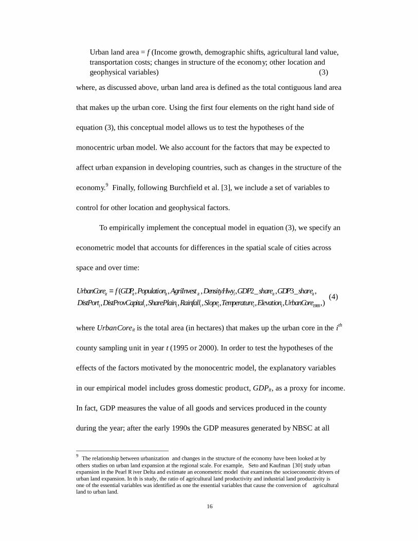
To empirically implement the conceptual model in equation (3), we specify an

econometric model that accounts for differences in the spatial scale of cities across

space and over time:

1988

( , , , , 2_ , 3_ ,, , , , , , , ,)

it it it it i it it

i i i i i i i

UrbanCore f GDP Population AgriInvest DensityHwy GDP share GDP shareDistPort DistProvCapital SharePlain Rainfall Slope Temperature Elevation UrbanCore

= (4)

where UrbanCoreit is the total area (in hectares) that makes up the urban core in the ith

county sampling unit in year t (1995 or 2000). In order to test the hypotheses of the

effects of the factors motivated by the monocentric model, the explanatory variables

in our empirical model includes gross domestic product, GDPit, as a proxy for income.

In fact, GDP measures the value of all goods and services produced in the county

during the year; after the early 1990s the GDP measures generated by NBSC at all

9 The relationship between urbanization and changes in the structure of the economy have been looked at by others studies on urban land expansion at the regional scale. For example, Seto and Kaufman [30] study urban expansion in the Pearl R iver Delta and estimate an econometric model that examines the socioeconomic drivers of urban land expansion. In th is study, the ratio of agricultural land productivity and industrial land productivity is one of the essential variables was identified as one the essential variables that cause the conversion of agricultural land to urban land.

17

levels of statistical data collection (county, province and national) are consistent

across administrative districts.10 We also include population, Populationit, for each

county. These data include non-rural and rural residents who have their official

residence permit (hukou) in the county sampling unit (regardless of whether they

reside in the urban core or not). People from other counties that have not officially

moved their hukou or who have not registered with the local bureau of public security

are not included.11 Unfortunately, no direct measure of agricultural rent or

commuting cost per mile exists for entire China over time. As a proxy for agricultural

rent, we include a measure of the amount of investment allocated to agriculture

(AgriInvestit). The idea of including this variable is that such investment could lead to

higher productivity in agriculture, hence increasing the opportunity cost of converting

to urban area. If a land market exists, the higher productivity should be capitalized

into land rental. In addition, as a proxy for commuting costs, we include highway

density (HwyDensityi). The underlying assumption is that investments in highways

make traveling faster and more convenient, which reduces the cost of commuting and

enables residents to enjoy cheaper housing in the suburbs while paying lower

commuting costs. As a result, we would expect that the demand for suburban locations

increases as commuting costs fall and hence leads to spatial growth of the urban area.

With the exception of highway density, all of these variables—urban core, income,

10 The correlation coefficient between GDP per capita and income per capita in the years and areas which have both measures is 0. 853. 11 Because of the nature of China’s population statistics, this is the only measure that i s available. As such, it differs from the measures used in other empirical studies (which typical are based on census district data —and so the measure of the size of population of the urban area is relati vely more accurate. However, sin ce by far the largest share of the non -rural populat ion in a county is in the urban settlements (our guess: around 90%), the measurement of the urban population in the urban core will not be that bad. To the extent that there is measurement error, it could be that the estimat ed coefficients could be underestimated [4].

18

population and agricultural land value—vary over time (that is, we have information

for both 1995 and 2000).

Given the rapid structural change taking place in developing countries and the

impact of these shifts on urbanization, as in Seto and Kaufman [30] and Burchfield et

al. [3], we also include measures to control for industrialization. Our measure of

industrialization is constructed as the value of GDP created in the industrial sector

divided by total GDP (GDP2_shareit). In China’s statistical data the sectors

considered as part of industry include manufacturing, construction, transportation and

communication and commerce. A similar measure was created for the service sector

(GDP3_shareit). The sectors considered as part of the service category include

transport, postal and telecommunication services, wholesale, retail trades and catering

services. Data are available for 1995 and 2000 for both of these variables.

Finally, following Burchfield et al. [3], we also control for climatic and

geophysical variables. In our data set none of these variables vary over time. First, we

include two climatic variables. Measures of average annual rainfall in a county over a

50 year period, 1950 to 2000 (Rainfalli) and average annual air temperature

(Temperaturei) are calculated as the sum of daily average temperature in a county over

a 50 year period, 1950 to 2000. Readings are available for over 400 national

meteorological stations. We use these readings and China-specific climate

interpolation models to interpolate the data from specific meteorological stations,

changing them into spatial data (at the 1x1 kilometer level) and then aggregating them

to county sampling units. Second, we also include three terrain variables. The first,

19

Elevationi, is measured as the average elevation of the county’s entire land area (both

urban core and non-urban core area). Slopei is the average slope of a county and is

intended to measure the steepness of a county’s hills and mountains. SharePlaini is a

variable that is created by dividing the land area in a county that has a slope that is

less than eight degrees by the total land area of the county. Taken together, these three

variables provide a control for the ruggedness of a county’s terrain, which should be

correlated with the difficulties of constructing urban infrastructure and buildings.

Finally, two variables, both in kilometers, control for the distance from county

sampling units to specific types of locations. DistPorti measures the distance to the

nearest port city; and DistProvCapitali measures the distance to the capital of the

province to which the county belongs. In addition to the economic and geophysical

variables of interest, the model includes a measure of urban core area in 1988

(Urban1988) in order to control for the overall size of the county sampling unit.

Accounting for Unobservables: First-Differences Model

While the specifications in equations (3) and (4) contain the elements that will

allow us to examine the determinants of changes to the urban core in China’s counties,

it is possible that the presence of certain unobserved or unmeasured factors which are

correlated with city size and one or more of the explanatory factors may be affecting

the sign, significance and/or magnitude of the coefficients of interest. For example,

one city may have an inherent attractiveness as a place to live and work due to its

history and culture, or due to general expectations about its future growth prospects.

We have two options to account for these factors. The first is to specify the model as a

20

fixed effects model by including county-level dummy variables county(D )i , which

involves creating and including over 2000 indicator variables (one for each county

analytical unit minus one). By doing so, unlike previous empirical attempts to model

urban area, we capture the time-invariant unobservable factors for each county.12 We

also (like McGrath [18]) include a time dummy (Year2000=1, for all observations

from 2000 and zero for observations from 1995) to account for time trends that are

common across all counties. When doing this, the new model for explaining urban

core expansion is:

county( , , , 2_ , 3_ ,D )it it it it it it iUrbanCore f GDP Population AgriInvest GDP share GDP share= (5)

Equation (5) differs from equation (4) in two fundamental ways. First, Dicounty are

added to the specification. Second, all variables that do not vary over time (or all

variables that do not have a t subscript in equation 4) are subsumed in the county

dummies. Note, that in adopting this framework, since our measure of transportation

cost does not vary over time, we are unable to test for this hypothesis, although all

time invariant transportation characteristics are controlled for.

Alternatively, it is possible to respecify equation (5) as a first-differences

model. This is done by redefining the five time variant variables in equation (5),

subtracting the observation from 1995 from the observation from 2000. The

redefinition creates a set of five new differenced variables that are noted by a delta

sign preceding the variable name. After doing so, the model to be estimated becomes:

12 To the extent that there are omitted variables that ar e correlated with our variables of interest, the estimated coefficients will be biased and the analysis based on the results may be misleading. Although to our knowledge there are no national -level analyses that are testing the monocentric model that include fixed effects, such a problem is noted in the work of Seto and Kauffman [30].

21

i i i i i iUrbanCore f ( GDP , Population , AgriInvest , GDP2 _ share , GDP3_ share )∆ = ∆ ∆ ∆ ∆ ∆ (6)

Although the results from equation (5) and equation (6) will be exactly the same, the

number of observations is exactly half, the county dummy variables are no longer

needed and the degrees of freedom are exactly the same. In the next section, we only

report the results from the first-differences model.

Results of the Multivariate Analysis

The role of the factors identified by the monocentric model in the expansion of

the urban core is clear when we estimate equation (2). Holding constant the area of

the urban core in 1988, the importance of GDP (or income) in explaining the

expansion of the urban core in the late 1990s is seen by its positive and highly

significant coefficient when it is added by itself (Table 2, column 1). The magnitude

of the coefficient, 0.397, intuitively means that as GDP grows by 10 percent (for

example), the urban core expands by 3.97 percent. Moreover, even as we

incrementally add other key variables in the modified monocentric model—

Population in column (2), AgriInvest in column (3), HwyDensity in column (4)—as

well as measures of industrialization (GDP2_share) and the rise of the service sector

(GDP3_share) in column (4), the importance of GDP growth remains. When adding

these variables, the magnitude of the coefficient changes little, only falling from 0.397

in column 1 to 0.344 while remaining significant statistically (column 5). The high

adjusted R-squares in columns (1) to (5) also illustrates that income, by itself (holding

constant the urban core in 1988), and in concert with the rest of the variables raised in

the monocentric model, can explain a large amount of the variability of the expansion

22

of the urban core. If these results were to hold up throughout our analysis, clearly

income is an important force that is expanding the urban core.

Our results also show that, holding GDP constant, demographic, agricultural

land values and transportation costs—the other variables in the traditional

monocentric model—are significant statistically with the expected signs. When only

considering economic factors (and not considering any geophysical factors),

Population is significant and positive when added by itself (column 2) and together

with the other economic variables (columns 3-5). The elasticity, however, is lower

ranging between 0.057 and 0.115. In contrast, the sign on the coefficient of the

AgriInvest variable, our proxy for agricultural land values, is negative and is in

accordance with the monocentric model. Ceteris paribus, the higher the land values,

the slower the expansion of the urban core. The coefficient on the transportation cost

variable, proxied by the density of the highway network (HwyDensity), is positive

which is also as expected. When transportation networks are well developed (or

dense), the cost of transportation is low and the urban core should be expected to

expand relatively more. Hence, when using an OLS estimator, like McGrath [5], the

coefficients on the key variables of interest have the expected sign and are significant.

Interestingly, in this relatively parsimonious model (that is, without controls

for geographic variables) the coefficients on the variables that we have added (in

addition to the variables in the traditional monocentric model) to make the model

more appropriate for understanding the spatial scale of cities in developing countries

also are consistent with our expectations. Specifically, the coefficient on the

23

industrialization variable (GDP2_share) is positive and significantly different than

zero (column 5). Likewise, the rise of the service sector (GDP3_share) is positive and

significant. In the OLS version of the model, while it may be somewhat surprising

that the coefficient on the industrialization variable is smaller than that on the service

sector variable, it could be that, in fact, growth in the service sector actually requires

more land (it increased its share of GDP by 4 percentage points in our sample to only

1 percentage point for industrialization). Together, the signs and significance of all of

these variables in our analysis suggest that, although complex, variables of the

monocentric model—both those related to the economy and demography—are useful

in explaining the spatial scale of cities in developing countries (including China).

Even when geophysical factors are added to the model in columns (6) and (7),

all of the coefficients of the variables from the modified monocentric model retain

their same signs. The magnitudes of the coefficients and levels of statistical

significance also are almost the same. Most conspicuously, when all of the

geophysical variables (distance, terrain and climate variables) are added, the

coefficient of the GDP variable, while still positive and significant, falls by 4

percentage points (from 0.351 to 0.308—about 12 percent). At the same time, the

coefficient on the Population and GDP3_share become larger and GDP2_share

becomes significant. The lesson from this part of the analysis is that when attempting

to measure the effect of economic/demographic variables on urban core expansion, it

is important to consider the effect of geophysical factors. Without accounting for them

the coefficients of the variables of interest are subject to modest omitted variable bias.

24

An even more important lesson about the process of building a model of urban

core expansion is seen by comparing columns (6), the model with economic and

geophysical factors, and column (7), the model with only geophysical factors. In the

same way that the magnitudes of the signs of the economic variables changed between

models with and without geophysical factors, the signs on the coefficients of the

geophysical factors change when economic factors are added or deleted. In fact, the

magnitude of the changes (in percentage terms) for many of the variables is much

higher (in absolute value terms). Most coefficients change significantly. Geographical

variables play an important role in explaining differences across space in urban core

expansion, but to more precisely measure their impacts, the effects of economic

variables are needed to be controlled for likely because of their powerful role in

pushing the boundaries of the urban core.

First Differencing: Accounting for Fixed Effects

When moving from Table 2 to Table 3, the hazard of estimating the

determinants of urban area in an estimation framework that does not control for all

fixed effects is seen. Most prominently the coefficients of all time-varying variables in

the first-differences model—which are all of the economic/demographic variables in

the monocentric model except the transportation cost variable—are significantly

different. Specifically, in the case of population, agricultural investment and

GDP2_share, the coefficients become insignificant from zero. While the coefficients

of the other variables—income and GDP3_share—are significant in all of models

(columns 1-4), their magnitudes are much lower.

25

The largest absolute drop in magnitude occurs in the case of GDP. The

coefficient on GDP remains significant throughout all of the specifications in Table 3.

Its magnitude, however, is much smaller. The magnitude of the elasticity of urban

core expansion with respect to GDP falls to less than 1/4 of what it was in Table 2,

(from 0.308 to 0.070). According to Table 3, if GDP (or income) increased by 10

percent, the urban core area would only increase by less than 1 percent (0.7 percent).

Interestingly, in the first-differences model, the effects of population and the

expansion of the industrial sector (GDP2_share) also fall sharply. The insignificant

signs, among other things, may mean that the expansion of the urban core is not being

driven by rising population or industrialization per se, but rather is the result of the

rapid income growth process. Hence, besides the contribution of the service sector,

the differences in the expansion of urban core only are being explained by differences

across counties in income growth rates. In China (at this point in its development)

income growth may be the driver of the rise of the spatial scale of the urban core.13

Decomposition Analysis

When using the approaches of previous work, we find that our ranking of the

importance of determinants of the spatial size of cities has similarities to previous

work. In earlier work, Brueckner and Fansler [2] concluded that the rankings were:

income, population, agricultural rents and transportation costs (although the last

variable was insignificant from zero). McGrath [18] found a different ranking:

13 The reader should be cautioned, h owever, that in this case the first d ifferences model is trying to estimate the change in the size of the urban core which has occurred only after five years. Since this period is a relatively short interval, these findings could differ if the exercise was conducted using data the spanned a g reater length of time. However, the sharp differences in the results at the very least should raise the question about how accounting for unobserved effects actually does affect the findings of work examining the determinants of the spatial size of cities.

26

population, income, transportation costs and agricultural rents. It should be noted that

in the case of these earlier empirical works ranked the importance of variables by the

size of their elasticities. If we had ranked our variables by the size of the elasticities

using the OLS results (from column 4) our rankings are: income, population,

agricultural land values (or investment in agriculture) and transportation cost

(highway density), which is the same as Breuckner and Fansler [2].

However, using the sizes of elasticities as criteria for determining the

importance of factors that cause shifts in the size of the urban core over time can be

deceiving. Elasticities are marginal measures. The total effect of a factor on the

change of another variable over time depends on both the size of the elasticity and

size of the change in the variable. In other words, even if an elasticity ε =dY/dX*X/Y

is large, if X does not change much over the time that we are measuring the change in

Y, X will contribute only marginally to the total change in Y. Decomposition analysis

is a better way to rank the importance of elements in a set of explanatory variables in

the change of a variable of interest (some Y) since they account for both the size of

the marginal effects and the size of the change of the explanatory variables.

The decomposition results (Table 4), which use the results from the fixed

effects models in Table 3, confirm the findings of the descriptive and regression

analyses.14 Growth (or income) is by far the most important factor affecting growth.

14 We could have used GDP per capita in our specificat ion instead of GDP. If we would have, the pop ulation variable’s coefficient, instead of being statistically zero, would have been positive and statistically different from zero (0.082). In fact, if we h ad specifie d the equation this way, the elastic ity on population would have been larger than the elast icity on GDP (which would have been exactly the same; as would all of the other elasticities). However, in an alternative decomposition because the change in population is so small (at least relative to the change in GDP/capita), the final decomposition would have differed little. It could also be that the m agnitude of the population variable is underestimated d ue to measurement error (as discussed in footnote 11).

27

It explains 121 percent of the spatial growth of the urban core (Table 4). What this

means is that urban core “should” have increased by 4.905 with 70.08 percent

increase of GDP. In fact, the urban core actually only expanded by 4.05 percent. In

other words, other (unmeasured) factors that must have slowed urban core expansion.

While all of the other time-varying economic factors (except agricultural

investment), including changes in population growth, expansion of industrialization

and the rise of the service sector, positively influence urban core expansion, their joint

impact is small (Table 4). The effects of population and the expansion of

industrialization and the service sector are all positive, but jointly they only explain

1.5 percent of the growth in the urban core. The overall process of income growth

completely dominates. The importance of using the first-differences model also

becomes clear in this case. Even with this smaller coefficient (from Table 3 instead of

Table 2), growth in GDP (income) explains all of urban expansion. If we would have

used the coefficient of the growth variable from the OLS equation in Table 2 (any of

the columns), it would have implied that, due to growth, the cities should have grown

by more than they actually did. Such a finding is not believable and it reinforces the

need to carefully model the impact of economic factors on urban core expansion.

Conclusion

In this paper we have shown that the monocentric model when applied to

developing countries—in this case China—has fairly high explanatory power and

produce results strikingly similar to analyses in the past. When we use specifications

that were used in the literature on the US, we find evidence that all of the hypotheses

28

of the standard monocentric model are valid. Income, population and transportation

costs positively affect the spatial size of the urban cores of China’s cities. Agricultural

rents detract from the expansion of the urban core.

Although we have not accounted explicitly for policy (mainly due to the lack

of a good set of measures), the decomposition results suggest that something apart

from the economic factors included in the first-differences model slowed the growth

of the urban core. Had it not been for these factors embodied in the residual, the urban

core would have been 22 percent larger. While it is impossible to interpret precisely

the meaning of the residual, it is possible to speculate that policy may have played a

role in slowing growth.

Methodologically, our paper suggests that in the future economists must utilize

urban spatial and economic/demographic data over time in the analysis of the

determinants of urban land size and more precisely decompose the changes in the

spatial size of cities. Although the time interval between the observations (5years) is

short, our results suggest that when time series are available and a first-differences

model is used, the nature of the results might change. The magnitudes of many

variables fall and some of the coefficients become insignificant. One of the lessons of

this paper is that accounting for unobserved effects by using a fixed effects or

first-differences model may matter. The expansion of the urban core is a complex

process and it is difficult to include measures of all of the factors that affect the spatial

size of cities.

29

Be that as it may, whether using results from the OLS or first-differences

model, the paper demonstrates the powerful role that income growth has played in

shaping China’s current economy, including the spatial size of its cities. Moreover,

regardless of the empirical approach we also found that the role of the other factors in

China is relatively small—even when considered jointly. If our results are correct, this

suggests that if China wants to continue to grow at high rates of GDP growth, the

urban core may have to continue to expand. Since China’s modernization hopes are

tied to income growth, there will almost certainly be a lot more urbanization before

China becomes a modern nation.

30

Acknowledgment

Authors benefited greatly from the comments from Jan Brueckner and the two

anonymous referees. The authors would like to thank Jiyuan Liu for his support with

the remote sensing data. The financial supports from the National Natural Science

Foundation of China (70503025) and Chinese Academy of Sciences

(KSCX2-YW-N-039) are appreciated. Any remaining errors and omissions are wholly

the responsibility of the authors.

31

References: [1] W. Alonso, Location and land use, Harvard U niversity Press, Cambridge, MA, 1964. [2] J.K. Brueckner, and D.A. Fansler, The economics of urban sprawl: theor y and evidence on the spatial sizes of cities. The Review of Eocnomics and Statistics 65 (1983) 479-482. [3] M. Burch•eld, H.G. Overman, D. Puga, and M.A. Turner, Cause of Sprawl: A Portrait from Space. Quarterly Journal of Economics 121 (2006) 587 -633. [4] A. Deaton, The Analysis of Household Surveys: A M icroeconometric App roach to Development Policy. Published for the World Bank, The Johns Hopkins U niversity Press, Baltimore and London, 1996. [5] X. Deng, Y. Liu, T. Zhao, Study on the land-use change and its spatial distribution: a case study in Ankang District. Resources and Environ ment in the Yangtze Basin, 12 (2003) 522 - 528. [6] X. Deng, J. Liu, and D. Zhuang, Modeling the relationship of land use change and some geophysical indicators: a case study in the ecotone between agriculture and pasturing in Northern China. Journal of Geographical Sciences 12 (2002) 397 -404. [7] M. Fujita, and H. Ogawa, Multiple Equlibria and Structural Transition of non -Monocentric Urban Configurations. Regional Science and Urban Economics 18 (1982) 161 -196. [8] J. Garreau, Edge Cit y, Doubleday, New York, 1991. [9] S.P.S. Ho, and G.C.S. Lin, Emerging land markets in rural and urban China: Policies and practices. The China Quarterly (2003) 681 -707. [10] N. Harris, Urbanization, economic development and policy in developing countries. Habitat International l4 (1990) 3-42. [11] J. Huang, X. Deng, and S. Rozelle, Cultiva ted Land Conversion and Bioproductivity in China, Proceedings of SPIE 49th Annual Meeting, 5544 (2004) 135-148. [12] F. Jin, and J. Wang, Railway Network Expansion and Spatial Accessibilit y Analysis in China: 1996 - 2000. Acta Geographica Sinica 59 (2004) 293 - 302. [13] K. Kok, The role of population in understanding Honduran land use patterns Journal of Environmental Management 72 (2004) 73 -89. [14] X. Li, and A.G.-O. Yeh, Accuracy Improvement of Land Use Change Detecti on Using

32

Principal Components Analysis: A Case Study in the Pear River Delta. Journal of Remote Sensing 1 (1997) 282-289. [15] J. Liu, M. Liu, and X. Deng, The Land -use and land-cover change database and its relative studies in China. Chinese Geographical Science 12 (200 2) 114-119. [16] J. Liu, M. Liu, and D. Zhuang, Study on spatial pat tern of land-use change in China during 1995-2000. Science in China (Series D) 46 (2003) 373 -384. [17] J.F. McDonald, The identificati on of urban employment subcenters. Journal of Urban Economics 21 (1987) 242-258. [18] D.T. McGrath, More evidence on the spatial scale of cities. Journal of Urban Econ omics 58 (2005) 1-10. [19] C. Milesi, C.D. Elvidge, R.R. Nemani, and S.W. Running, Assessing the impact o f urban land development on net primary productivity in the southeastern United States. Remote Sensing of Environment 86 (2003) 401 - 410. [20] E.S. Mills, An aggregative model of resource allocation in a metropolitan area. American Economic Review, Papers and Proceedings 57 (1967) 197-210. [21] Ministry of Public Security of China, China counties and cities' population yearbook, Chinese Public Security University Press, Beijing, 1996. [22] Ministry of Public Security of China, China counties and cities' population yearbook, Chinese Public Security University Press, Beijing, 2001. [23] R.F. Muth, Cities and housing, University of Chicago Press, Chicago, IL, 1969. [24] National Fundamental Geographic Information System, Geocoding system of administrative zones of in 1995(GB 2260-1995), National Fundamental Geographic Information System, Beijing, 2000. [25] NBSC, China social-economic statistical yearbooks for China's counties and cities, China Statistics Press, Beijing, 2001. [26] J.F. Palmera, and J.R.-K. Lankhorst, Evaluating visible spatial diversity in the landscape. Landscape and Urban Planning 43 (1998) 65 -78. [27] G. Petrakos, Urbanization and international tr ade in developing countries. World Development 17 (1989) 1269 -1277. [28] P. Shi, P. Gong, X. Li, J. Chen, Y. Qi, and Y. Pan, Method and Practice of Study on Land Use

33

/ Land Cover Changes, Science Press, Beijing, 2000. [29] Y. Sato, and K. Yamamoto, Population concentration, urb anization, and demographic transition. Journal of Urban Economics 58 (2005) 45 -61. [30] K.C. Seto, and R.K. Kaufmann, Modeling the drivers of urban land use change in the Pearl River Delta, China: integrating remote sensing with socioeconomic data. Land Economics 79 (2003) 106-121. [31] W.S. Tang, Urban land development un der socialism: China bet ween 1947 and 1977. International Journal of Urban and Regional Research 18 (1994) 395 -415. [32] J.E. Vogelmann, D. Helder, R. Morfitt, M.J. Choate, J.W. Merchant, and H. Bulley, Effects of Landsat 5 Thematic Mapper and Landsat 7 Enhanced Thematic Mapper Plus radiometric and geometric calibrations and corrections on landscape characterization. Remote Sensing of Environment 78 (2001) 55 - 70. [33] W.C. Wheaton, A comparative static anal ysis of urban spatial structure. J ournal of Economic Theory 9 (1974) 223-237. [34] C.E. Woodcock, S.A. Macomber, M. Pax-Lenney, and W.B. Cohen, Monitoring large areas for forest change using Landsat: Generalization across space, time and Landsat sensors. Remote Sensing of Environment 78 (2001) 194 - 203.

34

Table 1. Changes of income, population and other explanatory factors associated with the monocentric model (plus the factors needed for the analysis of developing countries) and the rate of growth of the urban core in China between 1995 and 2000.

Items Relatively slow urban core growtha

Relatively high urban core growtha

Growth in GDP 70.1 78.4

Population growth 2.3 3.5

Agricultural investment 31.1 22.3

Highway Density 20.8 42.2

Industrial GDP growth 77.8 81.8

Growth of GDP from service sector

94.0 95.5

Note a: Relatively slow growth of the urban core is associated with the counties that are in the lowest quartile (experiencing growth of less than 0.02% per year between (1995 and 2000); Relatively high growth of the urban core is associated with the counties that are in the highest quartile (experiencing growth of more than 13.55% per year between (1995 and 2000)

35

Table 2. Ordinary Least Squares Estimator of the Expansion of the Spatial Size of China’s Cities.

Dependent variable: Ln(Urban core area) in hectares (1) (2) (3) (4) (5) (6) (7) Ln(GDP) 0.397

(47.81)*** 0.369

(30.61)*** 0.373

(29.33)*** 0.364

(27.80)*** 0.344

(21.12)*** 0.308

(18.28)***

Ln(population) 0.057 (3.47)***

0.091 (5.23)***

0.094 (5.34)***

0.115 (5.95)***

0.186 (9.61)***

Ln(AgriInvest) -0.017 (3.60)***

-0.016 (3.52)***

-0.016 (3.53)***

-0.012 (2.73)***

Ln(HwyDensity) 0.005 (3.07)***

0.004 (2.92)***

0.001 (3.07)***

0.016 (10.64)***

GDP2_share 0.103 (1.32)

0.178 (2.35)**

GDP3_share 0.315 (3.16)***

0.543 (5.60)***

Ln(urban core in 1988) 0.504 (69.78)***

0.501 (69.24)***

0.484 (64.07)***

0.483 (63.88)***

0.481 (63.61)***

0.438 (58.35)***

0.589 (79.74)***

Ln(DistPort) -0.015 (2.81)***

-0.050 (8.41)***

Ln(DistProvCapital) 0.002 (0.74)

0.006 (2.16)**

SharePlain 0.243 (6.18)***

0.489 (11.55)***

Ln(Rainfall) -0.150 (7.60)***

-0.073 (3.55)***

Ln(Slope) -0.037 (4.62)***

-0.026 (2.96)***

Ln(Temperature) -0.048 (1.55)

-0.280 (9.06)***

Ln(Elevation) 0.021 (3.05) ***

0.001 (0.10)

Constant -1.295 (15.97)***

-1.669 (12.52)***

-2.229 (14.83)***

-1.923 (12.70)***

-2.086 (13.21)***

-1.092 (4.63)***

1.295 (5.46)***

Observations 4482 4482 4482 4482 4482 4482 4482 Adj. R-squared 0.79 0.79 0.79 0.79 0.79 0.81 0.74

Note: t statistics in parentheses•* significant at 10%; ** significant at 5%; *** significant at 1%.

36

Table 3. Results from a First-Differences Model of the Expansion of the Spatial Size of China’s Cities with No Intercept Term.

Dependent variable: Ln(Urban core area (hectares)) (1) (2) (3) (4)

Ln(GDP) 0.082 (19.97)***

0.083 (19.60)***

0.082 (18.42)***

0.070 (13.09)***

Ln(Population) 0.006 (0.37)

0.011 (0.66)

0.012 (0.72)

Ln(AgriInvest) -0.006 (1.03)

-0.007 (1.29)

GDP2_share 0.035 (1.14)

GDP3_share 0.153 (5.10)***

Observations 4482 4482 4482 4482

Number of code 2241 2241 2241 2241

R-squared 0.15 0.15 0.15 0.15

Note: t statistics in parentheses, * significant at 10%; ** significant at 5%; *** significant at 1%.

37

Table 4. Decomposition analysis of the Sources Urban Core Expansion in China, 1995 to 2000.1

Variables

(1) Estimated parameter

(2) Percentage changes in variables

(3) Impact on urban core

(%)

(4) Contribution

(%)

Based on Table 3, column 4 GDP 0.07 70.08 4.905 121 Population 0.012 2.76 0.033 1 AgriInvest -0.007 2.89 -0.020 -0.5 GDP2_share 0.035 0.01 0.000 0.0 GDP3_share 0.153 0.04 0.006 0.2 Residual -0.87 -22 Urban Core 4.05 100 Note: For ratios of industrial or ser vice GDP, they are measured as changes in the ratios.

1 The decomposition analysis is conducte d as follows. We first calculate the percentage ch ange of each variable during 1995 throu gh 2000 (Column 2). We then multiply Column (2) by the parameters estimated from the fixed effects model (Column 1) to obtain the impact of each variable on urban core (Column 3). Finall y, we divide impact of each variable (Col umn 3) by the percentage change in urban core during this period (4.05) to obtain the contribution of each variable on change in urban core (Column 4).

38

1988 1995 2000

Shanghai

Panel A: Shanghai

1988 1995 2000

Kunming

Panel B: Kuming

1988 1995 2000

Yibin

Panel C: Yibin Data Source: Landsat TM/ETM images, Chinese Academy of Science Database

Figure 1. Maps showing expansion of urban core in Shanghai, Kunming and Yibin from 1988 to 2000.

39

Panel (A): Changes from 1988 to 1995.

Panel (B): Changes from 1995 to 2000.

Data Source: TM/ETM images, Chinese Academy of Science Database

Figure 2. Percentage changes in areas of urban core in each pixel in China, 1988 to 2000.