Growth or Glamour?Fundamentals and Systematic Risk in

Stock Returns

John Y. Campbell, Christopher Polk, and Tuomo Vuolteenaho1

First draft: September 2003This version: May 2005

1Campbell: Department of Economics, Littauer Center, Harvard University, CambridgeMA 02138, and NBER. Email john_campbell@harvard.edu. Polk: Kellogg School of Man-agement, Northwestern University, 2001 Sheridan Rd., Evanston, IL 60208. Email c-polk@kellogg.northwestern.edu. Vuolteenaho: Arrowstreet Capital, LP, 44 Brattle St., 5th ßoor,Cambridge MA 02138. Email tvuolteenaho@arrowstreetcapital.com. This material is based uponwork supported by the National Science Foundation under Grant No. 0214061 to Campbell.

Abstract

The cash ßows of growth stocks are particularly sensitive to temporary movementsin aggregate stock prices (driven by movements in the equity risk premium), whilethe cash ßows of value stocks are particularly sensitive to permanent movements inaggregate stock prices (driven by market-wide shocks to cash ßows.) Thus the highbetas of growth stocks with the market�s discount-rate shocks, and of value stockswith the market�s cash-ßow shocks, are determined by the cash-ßow fundamentals ofgrowth and value companies. Growth stocks are not merely �glamour stocks� whosesystematic risks are purely driven by investor sentiment. More generally, accountingmeasures of Þrm-level risk have predictive power for Þrms� betas with market-widecash ßows, and this predictive power arises from the behavior of Þrms� cash ßows.The systematic risks of stocks with similar accounting characteristics are primarilydriven by the systematic risks of their fundamentals.

JEL classiÞcation: G12, G14, N22

1 Introduction

Why do stock prices move together? If stocks are priced by discounting their cashßows at a rate which is constant over time, although possibly varying across stocks,then movements in stock prices are driven by news about cash ßows. In this casecommon variation in prices must be attributable to common variation in cash ßows.If discount rates vary over time, however, then groups of stocks can move togetherbecause of common shocks to discount rates rather than fundamentals. For example,a change in the market discount rate will have a particularly large effect on theprices of stocks whose cash ßows occur in the distant future (Cornell 1999, Dechow,Sloan, and Soliman 2004). In the extreme, irrational investor sentiment can causecommon variation in stock prices that is entirely unrelated to the characteristics ofcash ßows; Barberis, Shleifer, and Wurgler (2005) and Greenwood (2005) suggest thatthis explains the common movement of stocks that are included in the S&P 500 andNikkei indexes.

Common variation in stock prices is particularly important when it affects the mea-sures of systematic risk that rational investors use to evaluate stocks. In the CapitalAsset Pricing Model (CAPM), the risk of each stock is measured by its beta with themarket portfolio, and it is natural to ask whether betas are determined by shocks tocash ßows or discount rates (Campbell and Mei 1993). Recently, Campbell (1993,1996) and Campbell and Vuolteenaho (2004) have proposed a version of Merton�s(1973) Intertemporal Capital Asset Pricing Model (ICAPM), in which investors caremore about permanent cash-ßow-driven movements than about temporary discount-rate-driven movements in the aggregate stock market. In their two-beta model, therequired return on a stock is determined not by its overall beta with the market, butby its �bad beta� with market cash-ßow shocks that earns a high premium and its�good beta� with market discount rates that earns a low premium. Campbell andVuolteenaho (2004) Þnd empirically that value stocks have relatively high bad betaswhile growth stocks have relatively high good betas. The high average return onvalue stocks, which is anomalous in the CAPM (Ball 1978, Basu 1977, 1983, Rosen-berg, Reid, and Lanstein 1985, Fama and French 1992), is predicted by the two-betamodel.

This paper asks whether stocks� bad betas and good betas are determined bythe characteristics of their cash ßows, or whether instead they arise from the discountrates, possibly driven by sentiment, that investors apply to those cash ßows. We Þrst

1

study the common variation of growth and value stocks, and then we examine othercommon movements in stock returns that can be predicted using Þrm-level equitymarket and accounting data.

At least since the inßuential work of Fama and French (1993), it has been under-stood that value stocks and growth stocks tend to move together, so that an investorwho holds them (and/or shorts growth stocks) takes on a common source of risk. Anopen question is what drives these common movements. One view is that value andgrowth stocks are exposed to different cash-ßow risks. Fama and French (1996), forexample, argue that value stocks are companies that are in Þnancial distress and vul-nerable to bankruptcy. Campbell and Vuolteenaho (2004) suggest that growth stocksmight have speculative investment opportunities that will be proÞtable only if equityÞnancing is available on sufficiently good terms; thus they are equity-dependent com-panies of the sort modeled by Baker, Stein, and Wurgler (2003). According to thisfundamentals view, growth stocks move together with other growth stocks and valuestocks with other value stocks because of the fundamental characteristics of their cashßows, as would be implied by a simple model of stock valuation in which discountrates are constant.

The empirical literature contains some tantalizing evidence in support of the fun-damentals view. Fama and French (1995) document common variation in the prof-itability of value and growth stocks, Cohen, Polk, and Vuolteenaho (2004) Þnd thatvalue stocks� proÞtability covaries more strongly with market-wide proÞtability thandoes growth stocks� proÞtability, and Liew and Vassalou (2000) show that value-minus-growth returns covary with future macroeconomic fundamentals. Bansal,Dittmar, and Lundblad (2003, 2005) and Hansen, Heaton, and Li (2004) use econo-metric methods similar to those in this paper to show that value stocks� cash ßowshave a higher long-run sensitivity to aggregate consumption growth than do growthstocks� cash ßows.

An alternative view is that the stock market simply prices value and growthstocks differently at different times. Cornell (1999), for example, argues that growthstock proÞts accrue further in the future than value stock proÞts, so growth stocksare longer-duration assets whose values are more sensitive to changes in the marketdiscount rate. Barberis and Shleifer (2003) and Barberis, Shleifer, andWurgler (2005)argue that value stocks lack common fundamentals but are merely those stocks thatare currently out of favor with investors, while growth stocks are merely �glamourstocks� that are currently favored by investors. According to this view, changes in

2

the market�s mood or sentiment create correlated movements in the pricing of stocksthat investors favor or disfavor.

This paper sets up direct tests of the fundamentals view against the sentimentview, using several alternative approaches. In a Þrst test, we estimate a VAR inthe manner of Campbell (1991), Campbell and Mei (1993), and Vuolteenaho (2002)to break Þrm-level stock returns into components driven by cash-ßow shocks anddiscount-rate shocks. We aggregate the estimated Þrm-level shocks for those stocksthat are included in value and growth portfolios, and regress portfolio-level cash-ßowand discount-rate news on the market�s cash-ßow and discount-rate news to Þnd outwhether fundamentals or sentiment drive the systematic risks of value and growthstocks. According to our results, the bad beta of value stocks and the good beta ofgrowth stocks are both determined primarily by their cash-ßow characteristics.

In a second test, we regress the accounting proÞtability of value and growth port-folios, measured by portfolio-level return on equity (ROE), on the two componentsof the market return estimated by Campbell and Vuolteenaho (2004), lengtheningthe horizon to emphasize longer-term trends rather than short-term ßuctuations inproÞtability. We Þnd that the ROE of value stocks is more sensitive to the market�scash-ßow news than is the ROE of growth stocks, consistent with the Þndings ofCohen, Polk, and Vuolteenaho. More importantly, we are able to refute the pure-sentiment story by showing that the ROE of growth stocks is more sensitive to themarket�s discount-rate news than is the ROE of value stocks. We obtain similarresults when we replace the VAR-based news terms with simple proxies at the marketlevel also.

In a third test, we run cross-sectional regressions of realized Þrm-level betas ontoÞrms� book-market ratios. We Þnd that a Þrm�s book-market ratio predicts its badbeta positively and its good beta negatively, consistent with the results of Campbelland Vuolteenaho (2004). When we decompose each Þrm�s bad and good beta intocomponents driven by the Þrm�s cash-ßow news and discount-rate news, we Þnd thatthe book-market ratio primarily predicts the cash ßow component of the bad beta,not the discount-rate component.

All three approaches tell us that the systematic risks of value and growth stocksare determined by the properties of their cash ßows. These results have importantimplications for our understanding of the value-growth effect. While formal modelsare notably lacking in this area, any structural model of the value-growth effect mustrelate to the underlying cash-ßow risks of value and growth companies. Growth

3

stocks are not merely glamour stocks whose comovement is driven purely by correlatedsentiment. Our results show that there�s more to growth than just �glamour.�

While Campbell and Vuolteenaho (2004) concentrate on value and growth portfo-lios, their two-beta model has broader application. In the second part of this paperwe use cross-sectional stock-level regressions to identify characteristics of commonstocks that predict their bad and good betas. We look at market-based historicalrisk measures, the lagged beta and volatility of stock returns; at accounting-basedhistorical risk measures, the lagged beta and volatility of a Þrm�s return on assets(ROA); and at accounting-based measures of a Þrm�s Þnancial status, including itsROA, debt-asset ratio, and capital investment-asset ratio.

Accounting measures of stock-level risk are not emphasized in contemporary aca-demic research, but were sometimes used to evaluate business risk and estimate thecost of capital for regulated industries in the period before the development of theCAPM (e.g. Bickley 1959). Recently, Morningstar Inc. has used accounting data tocalculate costs of capital for individual stocks in the Morningstar stock rating system.Morningstar explicitly rejects the use of the CAPM and argues that accounting datamay reveal information about long-run risk, very much in the spirit of Campbell andVuolteenaho�s �bad beta�:

In deciding the rate to discount future cash ßows, we ignore stock-price volatility (which drives most estimates of beta) because we welcomevolatility if it offers opportunities to buy a stock at a discount to its fairvalue. Instead, we focus on the fundamental risks facing a company�sbusiness. Ideally, we�d like our discount rates to reßect the risk of per-manent capital loss to the investor. When assigning a cost of equity toa stock, our analysts score a company in the following areas: Financialleverage - the lower the debt the better. Cyclicality - the less cyclical theÞrm, the better. Size - we penalize very small Þrms. Free cash ßows -the higher as a percentage of sales and the more sustainable, the better.(Morningstar 2004.)

Even in the CAPM, accounting data may be relevant if they help one predict thefuture market beta of a stock. This point has been emphasized byMyers and Turnbull(1977) among others, and has inßuenced the development of industry risk models.Our cross-sectional regressions show that accounting data do predict market betas.

4

Importantly, however, some accounting variables have disproportionate predictivepower for bad betas, while lagged market betas and volatilities of stock returns havedisproportionate predictive power for good betas. This result implies that accountingdata are more important determinants of a Þrm�s systematic risk and cost of capitalin the two-beta model than in the CAPM.

Finally, we use the cross-sectional regression approach in combination with ourÞrm-level VAR methodology to predict the components of a Þrm�s bad and good betathat are determined by its cash ßows and its discount rates. We Þnd that stock-level characteristics generally predict the cash-ßow components of a Þrm�s bad andgood beta, not the discount-rate components. The systematic risks of stocks withsimilar accounting characteristics are primarily driven by the systematic risks of theirfundamentals, an important extension of our Þnding for growth and value stocks.

Both our portfolio analysis and our Þrm-level analysis are driven by a desire to un-derstand the risk characteristics of publicly traded companies. It is important to notethat those risks cannot be measured from the risk characteristics of dividend streamsto dynamic trading strategies. The dividends paid by a dynamically rebalanced port-folio strategy may vary because the dividends of the Þrms in the portfolio change, butthey may also vary if the stocks sold have systematically different dividend yields thanstocks bought at the rebalance. For example, consider a dynamic strategy that buysnon-dividend-paying stocks in recessions and dividend-paying stocks in booms. Thedividends earned by this dynamic trading strategy will have a strong business-cyclecomponent even if the dividends of all underlying companies do not.

Therefore, any sensible attempt to measure the risks of Þrms� cash ßows at aportfolio level must use a �three-dimensional� data set, in which portfolios are formedeach year and then those portfolios are followed into the future for a number ofyears without rebalancing. Such three-dimensional data sets have been used byFama and French (1995) and Cohen, Polk, and Vuolteenaho (2003, 2004). We followthis methodology, and perform all our tests either at the Þrm level or using three-dimensional data sets that follow the cash ßows of a particular portfolio through timewithout rebalancing.

The remainder of the paper is organized as follows. Section 2 motivates ourempirical tests. Section 3 describes our aggregate and Þrm-level data, and section 4presents aggregate and Þrm-level VAR estimates. Section 5 presents our empiricalresults on growth and value portfolios, section 6 discusses cross-sectional regressionsusing Þrm-level characteristics to predict good and bad betas, and section 7 concludes.

5

2 A Decomposition of Stock Returns

2.1 Two components of the stock return

The price of any asset can be written as a sum of its expected future cash ßows,discounted to the present using a set of discount rates. The price of the asset changeswhen expected cash ßows change, or when discount rates change. This holds true forany expectations about cash ßows, whether or not those expectations are rational, butÞnancial economists are particularly interested in rationally expected cash ßows andthe associated discount rates. Even if some investors have irrational expectations,there should be other investors with rational expectations, and it is important tounderstand asset price behavior from the perspective of these investors.

There are at least two reasons why it is interesting to distinguish between assetprice movements driven by rationally expected cash ßows, and movements drivenby discount rates. First, investor sentiment can directly affect discount rates, butcannot directly affect cash ßows. Price movements that are associated with changingrational forecasts of cash ßows may ultimately be driven by investor sentiment, butthe mechanism must be an indirect one, for example working through the availabilityof new Þnancing for Þrms� investment projects. (See Subrahmanyam and Titman,2001, for an example of a model that incorporates such indirect effects.) Thus bydistinguishing cash-ßow and discount-rate movements we can shrink the set of possibleexplanations for asset price ßuctuations.

Second, conservative long-term investors should view returns due to changes indiscount rates differently from those due to changes in expected cash ßows. A loss ofcurrent wealth caused by an increase in the discount rate is partially compensated byimproved future investment opportunities, while a loss of wealth caused by a reductionin expected cash ßows has no such compensation. The difference is easiest to seeif one considers a portfolio of corporate bonds. The portfolio may lose value todaybecause interest rates increase, or because some of the bonds default. A short-horizoninvestor who must sell the portfolio today cares only about current value, but a long-horizon investor loses more from default than from high interest rates. Campbell(1993, 1996) and Campbell and Vuolteenaho (2004) use this insight to develop anempirical implementation of Merton�s (1973) ICAPM, in which investors with riskaversion greater than one demand a greater reward for bearing cash-ßow risk thanfor bearing discount-rate risk.

6

Campbell and Shiller (1988a) provide a convenient framework for analyzing cash-ßow and discount-rate shocks. They develop a loglinear approximate present-valuerelation that allows for time-varying discount rates. Linearity is achieved by ap-proximating the deÞnition of log return on a dividend-paying asset, rt+1 ≡ log(Pt+1+Dt+1)−log(Pt), around the mean log dividend-price ratio, (dt − pt), using a Þrst-orderTaylor expansion. Above, P denotes price, D dividend, and lower-case letters logtransforms. The resulting approximation is rt+1 ≈ k+ρpt+1+(1−ρ)dt+1−pt ,whereρ and k are parameters of linearization deÞned by ρ ≡ 1

±¡1 + exp(dt − pt)

¢and

k ≡ − log(ρ)− (1− ρ) log(1/ρ− 1). When the dividend-price ratio is constant, thenρ = P/(P +D), the ratio of the ex-dividend to the cum-dividend stock price. Theapproximation here replaces the log sum of price and dividend with a weighted aver-age of log price and log dividend, where the weights are determined by the averagerelative magnitudes of these two variables.

Solving forward iteratively, imposing the �no-inÞnite-bubbles� terminal conditionthat limj→∞ ρj(dt+j − pt+j) = 0, taking expectations, and subtracting the currentdividend, one gets

pt − dt = k

1− ρ +Et∞Xj=0

ρj[∆dt+1+j − rt+1+j] , (1)

where∆d denotes log dividend growth. This equation says that the log price-dividendratio is high when dividends are expected to grow rapidly, or when stock returns areexpected to be low. The equation should be thought of as an accounting identityrather than a behavioral model; it has been obtained merely by approximating anidentity, solving forward subject to a terminal condition, and taking expectations.Intuitively, if the stock price is high today, then from the deÞnition of the returnand the terminal condition that the dividend-price ratio is non-explosive, there musteither be high dividends or low stock returns in the future. Investors must then expectsome combination of high dividends and low stock returns if their expectations areto be consistent with the observed price.

Campbell (1991) extends the loglinear present-value approach to obtain a decom-position of returns. Substituting (1) into the approximate return equation gives

rt+1 − Et rt+1 = (Et+1 − Et)∞Xj=0

ρj∆dt+1+j − (Et+1 − Et)∞Xj=1

ρjrt+1+j (2)

= NCF,t+1 −NDR,t+1,

7

whereNCF denotes news about future cash ßows (i.e., dividends or consumption), andNDR denotes news about future discount rates (i.e., expected returns). This equationsays that unexpected stock returns must be associated with changes in expectationsof future cash ßows or discount rates. An increase in expected future cash ßows isassociated with a capital gain today, while an increase in discount rates is associatedwith a capital loss today. The reason is that with a given dividend stream, higherfuture returns can only be generated by future price appreciation from a lower currentprice.

If the decomposition is applied to the returns on the investor�s portfolio, thesereturn components can also be interpreted as permanent and transitory shocks to theinvestor�s wealth. Returns generated by cash-ßow news are never reversed subse-quently, whereas returns generated by discount-rate news are offset by lower returnsin the future. From this perspective it should not be surprising that conservativelong-term investors are more averse to cash-ßow risk than to discount-rate risk.

2.2 Measuring the components of returns

An important issue is how to measure the shocks to cash ßows and to discount rates.One approach, introduced by Campbell (1991), is to estimate the cash-ßow-news anddiscount-rate-news series using a vector autoregressive (VAR) model. This VARmethodology Þrst estimates the terms Et rt+1 and (Et+1−Et)

P∞j=1 ρ

jrt+1+j and thenuses realization of rt+1 and equation (2) to back out the cash-ßow news. This practicehas an important advantage � one does not necessarily have to understand the short-run dynamics of dividends. Understanding the dynamics of expected returns isenough.

When extracting the news terms in our empirical tests, we assume that the dataare generated by a Þrst-order VAR model

zt+1 = a+ Γzt + ut+1, (3)

where zt+1 is a m-by-1 state vector with rt+1 as its Þrst element, a and Γ are m-by-1vector and m-by-m matrix of constant parameters, and ut+1 an i.i.d. m-by-1 vectorof shocks. Of course, this formulation also allows for higher-order VAR models via asimple redeÞnition of the state vector to include lagged values.

Provided that the process in equation (3) generates the data, t+ 1 cash-ßow and

8

discount-rate news are linear functions of the t+ 1 shock vector:

NDR,t+1 = e10λut+1, (4)

NCF,t+1 = (e10 + e10λ) ut+1.

Above, e1 is a vector with Þrst element equal to unity and the remaining elementsequal to zeros. The VAR shocks are mapped to news by λ, deÞned as λ ≡ ρΓ(I −ρΓ)−1. e10λ captures the long-run signiÞcance of each individual VAR shock todiscount-rate expectations. The greater the absolute value of a variable�s coeffi-cient in the return prediction equation (the top row of Γ), the greater the weight thevariable receives in the discount-rate-news formula. More persistent variables shouldalso receive more weight, which is captured by the term (I − ρΓ)−1.

2.3 Decomposing betas

Previous empirical work uses Campbell�s (1991) return decomposition to investigatebetas in several different ways. Campbell and Mei (1993) break the returns onstock portfolios, sorted by size or industry, into cash-ßow and discount-rate com-ponents. They ask whether the betas of these portfolios with the return on themarket portfolio are determined primarily by their cash-ßow news or their discount-rate news. That is, for portfolio i they measure the cash-ßow news Ni,CF,t+1 and the(negtive of) discount-rate news −Ni,DR,t+1, and calculate Cov(Ni,CF,t+1, rM,t+1) andCov(−Ni,DR,t+1, rM,t+1). Campbell and Mei deÞne two beta components

βCFi,M ≡ Covt(Ni,CF,t+1, rM,t+1)

Vart¡rM,t+1

¢ (5)

and

βDRi,M ≡Covt(−Ni,DR,t+1, rM,t+1)

Vart¡rM,t+1

¢ , (6)

which add up to the traditional market beta of the CAPM,

βi,M = βCFi,M + βDRi,M . (7)

In their empirical implementation, Campbell and Mei assume that the conditionalvariances and covariances in (5) and (6) are constant. However, they do not lookseparately at the cash-ßow and discount-rate shocks to the market portfolio.

9

Campbell and Vuolteenaho (2004), by contrast, break themarket return into cash-ßow and (negative of) discount-rate news NM,CF,t+1 and −NM,DR,t+1. They measurecovariances Cov(ri,t+1, NM,CF,t+1) and Cov(ri,t+1,−NM,DR,t+1) and use these to deÞnecash-ßow and discount-rate betas,

βi,CFM ≡Covt (ri,t+1, NM,CF,t+1)

Vart¡rM,t+1

¢ (8)

and

βi,DRM ≡ Covt (ri,t+1,−NM,DR,t+1)Vart

¡rM,t+1

¢ , (9)

which again add up to the traditional market beta of the CAPM,

βi,M = βi,CFM + βi,DRM . (10)

Campbell and Vuolteenaho (2004) show that the ICAPM implies a price of riskfor βi,DRM equal to the variance of the return on the market portfolio, and a priceof risk for βi,CFM that is γ times higher, where γ is the coefficient of relative riskaversion of a representative investor. This leads them to call βi,DRM the �good� betaand βi,CFM the �bad� beta, where the latter is of primary concern to conservativelong-term investors. Empirically, Campbell and Vuolteenaho Þnd that value stockshave always had a considerably higher bad beta than growth stocks. This Þnding issurprising, since in the post-1963 sample value stocks have had a lower CAPM betathan growth stocks. The higher CAPM beta of growth stocks in the post-1963 sampleis due to their disproportionately high good beta. Campbell and Vuolteenaho alsoÞnd that these properties of growth and value stock betas can explain the relativeaverage returns on growth and value during this period.

In this paper we combine the asset-speciÞc beta decomposition of Campbell andMei (1993) with the market-level beta decomposition of Campbell and Vuolteenaho(2004). We measure four covariances and deÞne

βCFi,CFM ≡ Covt(Ni,CF,t+1, NM,CF,t+1)

Vart¡rM,t+1

¢ , (11)

βDRi,CFM ≡Covt(−Ni,DR,t+1, NM,CF,t+1)

Vart¡rM,t+1

¢ , (12)

10

βCFi,DRM ≡Covt(Ni,CF,t+1,−NM,DR,t+1)

Vart¡rM,t+1

¢ , (13)

and

βDRi,DRM ≡Covt(−Ni,DR,t+1,−NM,DR,t+1)

Vart¡rM,t+1

¢ . (14)

These four beta components add up to the overall market beta,

βi,M = βCFi,CFM + βDRi,CFM + βCFi,DRM + βDRi,DRM . (15)

The bad beta of Campbell and Vuolteenaho can be written as

βi,CFM = βCFi,CFM + βDRi,CFM , (16)

while the good beta can be written as

βi,DRM = βCFi,DRM + βDRi,DRM . (17)

This four-way decomposition of beta allows us to ask whether the high bad beta ofvalue stocks and the high good beta of growth stocks are attributable to their cashßows or to their discount rates.

An interesting early paper that explores a similar decomposition of beta is Pettitand WesterÞeld (1972). Pettit and WesterÞeld use earnings growth as a proxy forcash-ßow news, and the change in the price-earnings ratio as a proxy for discount-rate news. They argue that stock-level cash-ßow news should be correlated withmarket-wide cash-ßow news, and that stock-level discount-rate news should be corre-lated with market-wide discount-rate news, but they assume zero cross-correlationsbetween stock-level cash ßows and market-wide discount rates, and between stock-level discount rates and market-wide cash ßows. That is, they assume βDRi,CFM =βCFi,DRM = 0 and work with an empirical two-way decomposition: βi,M = βCFi,CFM+βDRi,DRM . Comparing value and growth stocks, our subsequent empirical analysisshows that there is interesting cross-sectional variation in βCFi,DRM .

A very recent paper that explores the four-way decomposition of beta, written sub-sequent to the Þrst draft of this paper, is Koubouros, Malliaropulos, and Panopoulou(KMP, 2004). KMP estimates separate risk prices for each of the four components ofbeta. Consistent with the asset pricing theory of Campbell and Vuolteenaho (2004),KMP Þnds that risk prices are sensitive to the use of cash-ßow or discount-rate newsat the market level, but not at the Þrm or portfolio level.

11

3 Data

3.1 Aggregate VAR data

In specifying the aggregate VAR, we follow Campbell and Vuolteenaho (2004) bychoosing the same four state variables. However, unlike Campbell and Vuolteenaho,we implement the VAR using annual data in order to correspond to our estimation ofthe Þrm-level VAR, which is more naturally implemented using annual observations.

The aggregate-VAR state variables are deÞned as follows. First, the excess logreturn on the market (reM) is the difference between the annual log return on theCRSP value-weighted stock index (rM) and the annual log riskfree rate, constructedby CRSP as the return from rolling over Treasury bills with approximately threemonths to maturity. We take the excess return series fromProfessor Kenneth French�swebsite.

The term yield spread (TY ) is provided by Global Financial Data and is computedas the yield difference between ten-year constant-maturity taxable bonds and short-term taxable notes, in percentage points. Keim and Stambaugh (1986) and Campbell(1987) point out that TY predicts excess returns on long-term bonds. These papersargue that since stocks are also long-term assets, TY should also forecast excess stockreturns, if the expected returns of long-term assets move together. Fama and French(1989) show that TY tracks the business cycle, so this variable may also capturecyclical variation in the equity premium.

We construct our third variable, the smoothed price-earnings ratio (PE), as theprice of the S&P 500 index divided by a ten-year trailing moving average of ag-gregate earnings of companies in the index. Following Graham and Dodd (1934),Campbell and Shiller (1988b, 1998) and Shiller (2000) advocate averaging earningsover several years to avoid temporary spikes in the price-earnings ratio caused bycyclical declines in earnings. This variable must predict low stock returns over thelong run if smoothed earnings growth is close to unpredictable. As in Campbell andVuolteenaho (2004), we construct the earnings series to avoid any forward-lookinginterpolation of earnings, ensuring all components of the time t earnings-price ratioare contemporaneously observable. Finally, we log transform the simple ratio.

Fourth, we compute the small-stock value spread (V S) using the data made avail-

12

able by Professor Kenneth French on his web site. The portfolios, which are con-structed at the end of each June, are the intersections of two portfolios formed onsize (market equity, ME) and three portfolios formed on the ratio of book equityto market equity (BE/ME). The size breakpoint for year t is the median NYSEmarket equity at the end of June of year t. BE/ME for June of year t is the bookequity for the last Þscal year end in t − 1 divided by ME for December of t − 1.The BE/ME breakpoints are the 30th and 70th NYSE percentiles. At the end ofJune of year t, we construct the small-stock value spread as the difference betweenthe log(BE/ME) of the small high-book-to-market portfolio and the log(BE/ME)of the small low-book-to-market portfolio, where BE and ME are measured at theend of December of year t− 1.We include V S because of the evidence in Brennan, Wang, and Xia (2001), Camp-

bell and Vuolteenaho (2004), and Eleswarapu and Reinganum (2004) that relativelyhigh returns for small growth stocks predict low returns on the market as a whole.This variable can be motivated by the ICAPM itself. If small growth stocks havelow and small value stocks have high expected returns, and this return differentialis not explained by the static CAPM, the ICAPM requires that the excess returnof small growth stocks over small value stocks be correlated with innovations in ex-pected future market returns. There are other more direct stories that also suggestthe small-stock value spread should be related to market-wide discount rates. Onepossibility is that small growth stocks generate cash ßows in the more distant fu-ture and therefore their prices are more sensitive to changes in discount rates, justas coupon bonds with a high duration are more sensitive to interest-rate movementsthan are bonds with a low duration (Cornell 1999). Another possibility is that smallgrowth companies are particularly dependent on external Þnancing and thus are sen-sitive to equity market and broader Þnancial conditions (Ng, Engle, and Rothschild1992, Perez-Quiros and Timmermann 2000). Finally, it is possible that episodes ofirrational investor optimism (Shiller 2000) have a particularly powerful effect on smallgrowth stocks.

To ensure consistency with Campbell and Vuolteenaho�s (2004) study, we fol-low exactly their data construction steps. Consequently, our annual series of TY ,PE, and V S are exactly equal to corresponding end-of-May values in Campbell andVuolteenaho�s data set. We estimate the VAR over the period 1928-2001, with 74annual observations.

13

3.2 Firm-level VAR data

The raw Þrm-level data come from the merger of three databases. The Þrst of these,the Center for Research in Securities Prices (CRSP) monthly stock Þle, providesmonthly prices; shares outstanding; dividends; and returns for NYSE, AMEX, andNASDAQ stocks. The second database, the COMPUSTAT annual research Þle,contains the relevant accounting information for most publicly traded U.S. stocks.When using COMPUSTAT as our source of accounting information, we require thatthe Þrm must be on COMPUSTAT for two years. This requirement alleviates most ofthe potential survivor bias due to COMPUSTAT backÞlling data. The COMPUSTATaccounting information is supplemented by the third database, Moody�s book equityinformation for industrial Þrms as collected by Davis, Fama, and French (2000). Thisdatabase enables us to estimate the Þrm-level VAR over the period 1929-2001.

We implement the main speciÞcation of our Þrm-level VAR with the followingthree state variables. First, the log Þrm-level return (ri) is the annual log value-weight return on a Þrm�s common stock equity. Annual returns are compoundedfrom monthly returns, recorded from the beginning of June to the end of May. Wesubstitute zeros for missing monthly returns. Delisting returns are included whenavailable. For missing delisting returns where the delisting is performance-related,we assume a -30 percent delisting return, following Shumway (1997). Otherwise,we assume a zero delisting return. The log transformations of a Þrm�s stock returnmay turn extreme values into inßuential observations. We avoid this problem byunlevering the stock by 10 percent, that is, we deÞne the stock return as a portfolioconsisting of 90 percent of the Þrm�s common stock and a 10 percent investment inTreasury Bills.2

Our second Þrm-level state variable is the log book-to-market equity ratio (wedenote the transformed quantity by BM in contrast to simple book-to-market thatis denoted by BE/ME) as of the end of May in year t. We include BM in thestate vector to capture the well-known value effect in the cross section of averagestock returns (Graham and Dodd, 1934). In particular, we choose book-to-market asour scaled price measure based on the evidence in Fama and French (1992) that thisvariable subsumes the information in many other scaled price measures concerningfuture relative returns.

We measure BE for the Þscal year ending in calendar year t−1, andME (market2See Vuolteenaho (2002) for additional details and justiÞcation.

14

value of equity) at the end of May of year t.3 We require each Þrm-year observationto have a valid past BE/ME ratio that must be positive in value. Moreover, inorder to eliminate likely data errors, we censor the BE/ME variables of these Þrmsto the range (.01,100) by adjusting the book value. To avoid inßuential observationscreated by the log transform, we Þrst shrink the BE/ME towards one by deÞningBM ≡ log[(.9BE + .1ME)/ME].Third, we calculate long-term proÞtability, ROE, as the Þrm�s average proÞtability

over the last one to Þve years, depending on data availability. We generate ourearnings series using the clean-surplus relation. In that relation, earnings, dividends,and book equity satisfy

BEt −BEt−1 = Xt −Dnett :

book value today equals book value last year plus clean-surplus earnings (Xt) less(net) dividends. This approach is dictated by necessity (the early data consist ofbook-equity series but do not contain earnings). Note that in our data set, weconstruct clean-surplus earnings with an appropriate adjustment for equity offeringsso that

Xt =

∙(1 +Rt)MEt−1 −Dt

MEt

¸×BEt −BEt−1 +Dt,

where Dt is gross dividends, computed from CRSP. We deÞne ROE as the trailingÞve-year average earnings divided by the trailing Þve-year average of (.9BE+ .1ME).We choose ROE as the Þnal element of our Þrm-level state vector to capture the evi-dence that Þrms with higher proÞtability (controlling for their book-to-market ratios)have earned higher average stock returns (Haugen and Baker 1996, Kovtunenko andSosner 2003). Vuolteenaho (2002) uses just the previous year�s proÞtability in his

3Following Fama and French, we deÞne BE as stockholders� equity, plus balance sheet deferredtaxes (COMPUSTAT data item 74) and investment tax credit (data item 208) (if available), pluspost-retirement beneÞt liabilities (data item 330) (if available), minus the book value of preferredstock. Depending on availability, we use redemption (data item 56), liquidation (data item 10),or par value (data item 130) (in that order) for the book value of preferred stock. We calculatestockholders� equity used in the above formula as follows. We prefer the stockholders� equity numberreported by Moody�s, or COMPUSTAT (data item 216). If neither one is available, we measurestockholders� equity as the book value of common equity (data item 60), plus the book value ofpreferred stock. (Note that the preferred stock is added at this stage, because it is later subtractedin the book equity formula.) If common equity is not available, we compute stockholders� equity asthe book value of assets (data item 6) minus total liabilities (data item 181), all from COMPUSTAT.

15

Þrm-level VAR. We instead average over as many as Þve years of past proÞtabil-ity data due to the fact that unlike Vuolteenaho, we use much noisier clean-surplusearnings instead of GAAP earnings.

4 VAR Estimation

4.1 Aggregate VAR

Table 1 reports the VAR model parameters, estimated using OLS. Each row of thetable corresponds to a different equation of the VAR. The Þrst Þve columns reportcoefficients on the Þve explanatory variables: a constant, and lags of the excess marketreturn, term yield spread, price-earnings ratio, and small-stock value spread. OLSstandard errors are reported in parenthese below the coefficients.

The Þrst row of Table 1 shows that three out of our four VAR state variables havesome ability to predict annual excess returns on the aggregate stock market. Unlikein the monthly data which exhibits some degree of momentum, annual market returnsdisplay a modest degree of reversal; the coefficient on the lagged excess market returnis a statistically insigniÞcant -.0354 with a t-statistic of -.3. The regression coefficienton past values of the term yield spread is positive, consistent with the Þndings of Keimand Stambaugh (1986), Campbell (1987), and Fama and French (1989), though theassociated t-statistic of 1.4 is somewhat modest. The smoothed price-earnings rationegatively predicts the return with a t-statistic of 2.6, consistent with the Þndingthat various scaled-price variables forecast aggregate returns (Campbell and Shiller,1988ab, 1998; Rozeff 1984; Fama and French 1988, 1989). Finally, the small-stockvalue spread negatively predicts the return with a t-statistic of 2.1, consistent withBrennan, Wang, and Xia (2001) and Eleswarapu and Reinganum (2004). In sum-mary, the estimated coefficients, both in terms of signs and t-statistics, are generallyconsistent with our prior beliefs and Þndings in previous research.

The remaining rows of Table 1 summarize the dynamics of the explanatory vari-ables. The term spread can be predicted with its own lagged value and the laggedsmall-stock value spread. The price-earnings ratio is highly persistent, and approx-imately an AR(1) process. Finally, the small-stock value spread is also a highlypersistent AR(1) process.

16

The sixth column of Table 1 computes the coefficients of the linear function thatmaps the VAR shocks to discount-rate news, e10λ. We deÞne λ ≡ ρΓ(I−ρΓ)−1, whereΓ is the estimated VAR transition matrix from Table 1. Following Campbell andVuolteenaho (2004), we set ρ equal to .95 throughout the paper. Interestingly, thecoefficients of e10λ are very similar to those estimated by Campbell and Vuolteenahofrom monthly data, with the exception of the coefficient on stock-return shock, whichis larger in absolute value in the function computed from annual VAR parameterestimates. As a further robustness check, we compared our annual news terms tocorresponding twelve-month sums of Campbell and Vuolteenaho�s news terms andobserved a high degree of consistency (a correlation of .98 for NDR and .88 for NCF ).

The persistence of the VAR explanatory variables raises some difficult statisticalissues. It is well known that estimates of persistent AR(1) coefficients are biaseddownwards in Þnite samples, and that this causes bias in the estimates of predictiveregressions for returns if return innovations are highly correlated with innovations inpredictor variables (Stambaugh 1999). There is an active debate about the effectof this on the strength of the evidence for return predictability (Ang and Bekaert2003, Campbell and Yogo 2005, Lewellen 2004, Polk, Thompson, and Vuolteenaho2005, Torous, Valkanov, and Yan 2005). Our interpretation of the Þndings in thisliterature is that there is some statistical evidence of return predictability based onvariables similar to ours. However, an additional complication is that the statisticalsigniÞcance of the one-period return-prediction equation does not guarantee that ournews terms are not materially affected by the above-mentioned small-sample biasand sampling uncertainty. This is because the news terms are computed using acomplicated nonlinear transformation of the VAR parameter estimates.4 With thesecaveats, we proceed with news terms extracted using the point estimates reported inTable 1.

Figure 1 plots centered three-year moving averages of −NM,DR (line with squares)and NM,CF (thick solid line). Both moving-average series are normalized to have aunit standard deviation. The Þgure shows stock prices declining because of discount-rate news in the early 1930�s, late 40�s, late 60�s, mid 70�s, and early 80�s. Aggregatestock prices increased because of discount-rate news in the late 1930�s, early and mid60�s, and for a long period from the mid 1980�s to late 90�s. Good cash-ßow news wereexperienced in the period from the mid 1940�s to late 50�s, late 60�s, late 70�s, and

4The appendix to Campbell and Vuolteenaho (2004), available online athttp://kuznets.fas.harvard.edu/~campbell/papers/BBGBAppendix20040624.pdf, presents evi-dence that there is little Þnite-sample bias in the estimated news terms used in that paper.

17

90�s, while bad cash-ßow news dominate the 1930�s, early 70�s, and 80�s. Since we areinterested in separating the effects of discount-rate and cash-ßow news, the 1950�s, late70�s, and the period from the late 1980�s to early 90�s are all inßuental observationsduring which the two news terms pushed stock prices in opposite directions.

Table 2 puts these extracted news terms to work. In this table, we estimatethe good discount-rate betas (βi,DR) and bad cash-ßow betas (βi,CF ) for portfolios ofvalue and growth stocks. Each year, we form quintile value-weighted portfolios basedon Þrms� book-to-market ratios, and denote the extreme growth portfolio with 1 andthe extreme value portfolio with 5. When forming the portfolios we allocate an equalamount of market capitalization to each portfolio, in order to ensure that all the port-folios are economically meaningful.5 We regress these portfolios� simple returns on thescaled news seriesNM,DR×Var (reM) /Var(NM,DR) andNM,CF×Var (reM) /Var(NM,CF ).The scaling normalizes the regression coefficients to correspond to our deÞnitions ofβi,DR and βi,CF , which add up to the CAPM beta.

The point estimates in the second panel of Table 2 show that value stocks havehigher cash-ßow betas than growth stocks in the full sample as well as in both sub-periods. The estimated difference between the extreme growth and value portfolios�cash-ßow betas is -.13, and this difference is stable across subperiods. In contrast,the pattern in discount-rate betas changes from one subperiod to another. Growthstocks� discount-rate betas are signiÞcantly below one in the early subperiod and veryclose to one in the later subperiod. More striking is that value stocks� discount-ratebetas decline from 1.18 in the Þrst subsample to .48 in the second subsample. Overall,the return betas estimated from the annual data are consistent with those estimatedfrom monthly data by Campbell and Vuolteenaho (2004).

The full-period estimates of bad and good beta for the market portfolio sum up toapproximately one. Curiously, however, the sum of estimated bad and good betas isabove one for the Þrst subperiod and below one for the second subperiod. The factthat these subperiod betas deviate from one is caused by our practice of removingthe conditional expectation from the market�s return (NM,CF − NM,DR equals theunexpected return) but not from the test asset�s return. Because the aggregateVAR is estimated from the full sample, in the subsamples there is no guarantee thatthe estimated conditional expected return is exactly uncorrelated with unexpected

5The typical approach allocates an equal number of Þrms to each portfolio. Since growth Þrmsare typically much larger than value Þrms, this approach generates value portfolios that contain onlya small fraction of the capitalization of the market.

18

returns. Thus, in the subsamples, the expected test-asset return may contribute tothe beta, moving it away from unity.

The standard errors in Table 2, as well as the standard errors in all subsequenttables that use estimated news terms, require a caveat. We present the simple OLSstandard errors from the regressions, which do not take into account the estimationuncertainty in the news terms. Thus, while the t-statistics in Table 2 are generallyhigh in absolute value, the true statistical precision of these estimates is likely to belower.

4.2 Firm-level VAR

The Þrm-level VAR generates market-adjusted cash-ßow and discount-rate news foreach Þrm each year. Since relatively few Þrms survive the full time period; sinceconditioning on survival may bias our coefficient estimates; and since the averagenumber of Þrms we consider is greater than the number of annual observations, weassume that the VAR transition matrix is equal for all Þrms and estimate the VARparameters with pooled regressions.

We remove year-speciÞc means from the state variables by subtracting rM,t fromri,t and cross-sectional means from BMi,t and ROEi,t. Instead of subtracting theequal-weight cross-sectional mean from ri,t, we subtract the log value-weight CRSPindex return instead, because this will allow us to undo the market adjustment simplyby adding back the cash-ßow and discount-rate news extracted from the aggregateVAR.

After cross-sectionally demeaning the data, we estimate the coefficients of the Þrm-level VAR using WLS. SpeciÞcally, we multiply each observation by the inverse ofthe number of cross-sectional observation that year, thus weighing each cross-sectionequally. This ensures that our estimates are not dominated by the large cross sectionsnear the end of the sample period. We impose zero intercepts on all state variables,even though the market-adjusted returns do not necessarily have a zero mean in eachsample. Allowing for a free intercept does not alter any of our results in a measurableway.

Parameter estimates, presented in Table 3, imply that expected returns are highwhen past one-year return, the book-to-market ratio, and proÞtability are high.

19

Book-to-market is the statistically most signiÞcant predictor, while the Þrm�s ownstock return is the statistically least signiÞcant predictor. Expected proÞtability ishigh when past stock return and past proÞtability are high and the book-to-marketratio is low. The expected future book-to-market ratio is mostly affected by the pastbook-to-market ratio.

These VAR parameter estimates translate into a function e10λ that has positiveweights on all state-variable shocks. The t-statistics on the coefficients in e10λ are2.1 for past return, 2.6 for book-to-market, and 1.8 for proÞtability. Contrasting theÞrm-level e10λ estimates to those obtained from the aggregate VAR of Table 1, it isinteresting to note that the partial relation between expected-return news and stockreturn is positive at the Þrm level and negative at the market level. The positiveÞrm-level effect is consistent with the literature on momentum in the cross-section ofstock returns.

Table 3 also reports a variance decomposition for Þrm-level market-adjusted stockreturns. The total variance of the return is the sum of the variance of expected-return news (0.0048, corresponding to a standard deviation of 7%), the variance ofcash-ßow news (0.1411, corresponding to a standard deviation of 38%), and twice thecovariance between them (0.0046, corresponding to a correlation of 0.18). The totalreturn variance is 0.1551, corresponding to a return standard deviation of almost 40%.Thus the Þrm-level VAR attributes 97% of the variance of Þrm-level market-adjustedreturns to cash-ßow news, and only 3% to discount-rate news. If one adds back theaggregate market return to construct a variance decomposition for total Þrm-levelreturns, cash-ßow news accounts for 80% of the variance and discount-rate news for20%. This result, due originally to Vuolteenaho (2002), is consistent with a muchlower share of cash-ßow news in the aggregate VAR because most Þrm-level cash-ßownews is idiosyncratic, so it averages out at the market level.

The high share of cash-ßow news implied by the Þrm-level VAR results in partfrom the 1929-2001 sample period over which the VAR is estimated. In the onlineAppendix to this paper, Campbell, Polk, and Vuolteenaho (2005), we report Þrm-levelVAR estimates for the period 1963-2001. Over this period the VAR explanatory vari-ables are stronger predictors of market-adjusted Þrm-level stock returns. The impliedvariance of expected-return news is 0.025, corresponding to a standard deviation ofalmost 16%, and the variance of cash-ßow news is 0.166, corresponding to a standarddeviation of 41%. Although expected-return news is more volatile in the 1963-2001period, the beta patterns we discuss later in the paper are very similar.

20

We construct cash-ßow and discount-rate news for our BE/ME-sorted portfoliosas follows. We Þrst take the market-adjusted news terms extracted using the Þrm-level VAR in Table 3 and add back the market�s news terms for the correspondingperiod. This add-back procedure scales our subsequent beta estimates, but does notaffect the differences in betas between stocks. Then, each year we form portfolio-levelnews as the value-weighted average of the Þrms� news. The portfolios are constructedby sorting Þrms into Þve portfolios on their BE/ME�s each year. As before, we setBE/ME breakpoints so that an equal amount of market capitalization is in eachquintile each year. As a result, we have series that closely approximate the cash-ßowand discount-rate news on these quintile portfolios.

5 Beta Decomposition for Growth and Value Port-folios

5.1 VAR-based beta decomposition

Table 4 uses the portfolio-level and market-level news terms to decompose the CAPMbeta into four components: βCFi,CFM , βDRi,CFM , βCFi,DRM , and βDRi,DRM . For eachportfolio, we run four simple regressions, the portfolio-level news on scaled seriesNM,DR × Var (reM) /Var(NM,DR) and NM,CF ×Var (reM) /Var(NM,CF ). The portfolioi = 1 is the extreme growth portfolio (low BE/ME) and i = 5 the extreme valueportfolio (high BE/ME). In the table, �1-5� denotes the difference between extremegrowth (1) and value (5) portfolios.

Table 4 shows that the cross-sectional beta patterns visible in Table 2 are entirelydue to cross-sectional variation in Þrms� βCFi,CFM and βCFi,DRM . In other words,although the components βDRi,CFM and βDRi,DRM are important determinants ofthe overall level of betas, they are approximately constant across value and growthportfolios.

A caveat about the standard errors is in order. All standard errors in tables thatuse estimated news terms ignore the estimation uncertainty in extraction of the newsterms. Thus, the generally high t-statistics in Table 4 and the subsequent tablesmay be overstated.

21

While the simple regressions of Table 4 neatly correspond to the beta decompo-sition of economically interesting betas from the asset-pricing perspective, multipleregressions may be more appropriate in understanding the sources of these sensitivi-ties. Suppose that the technology employed by value and growth Þrms is such thatÞrms� cash ßows are determined by a constant linear function of the market-widediscount-rate and cash-ßow news, plus an error term. Then, the simple regres-sion coefficients (and thus our beta decomposition) may be subject to change as thecorrelation between the market�s news terms changes. In particular, the in-samplecorrelation of NM,CF,t+1 and−NM,DR,t+1 is positive in the early subsample but slightlynegative in the modern subsample.

To examine the partial sensitivity of Þrms� cash ßows to the market�s discount-rateand cash-ßow news, the left-hand panel of Table 5 regresses the portfolio-level cash-ßow news on the estimated −NM,DR,t+1 and NM,CF,t+1 in a multiple regression. Weshow results for three portfolios (1, 3, and 5) to save space. The multiple regressionstell an interesting story. In the full-period regressions, growth stocks� cash-ßow newsis more sensitive to −NM,DR,t+1 and less sensitive to NM,CF,t+1 than that of valuestocks.

In the subperiod analysis, the sensitivities of growth and value stocks� cash-ßownews to the market�s cash-ßow news appears to be roughly constant. (This is incontrast with the simple regression results, which are inßuenced by the sample-speciÞccorrelation of the market�s news terms.) The extreme growth stocks� cash-ßow newshas a .07 loading on the market�s cash-ßow news in the early subsample and .03 in thesecond subsample, while the extreme value stocks� cash-ßow news has a .13 loading onthe market�s cash-ßow news in the early subsample and .15 in the second subsample.Thus, the partial sensitivities to the market�s cash-ßow news seem to be relativelystable over time, with value stocks� sensitivity at a higher level than that of growthstocks.

The sensitivities of growth and value stocks� cash-ßow news to the market�s (nega-tive) discount-rate news appear to have changed across samples. In the early sample,value stocks� cash ßows seem to be slightly more sensitive to the market�s valuationlevels than growth stocks� cash ßows (1-5 difference -.11, t-stat -2.0). In the mod-ern subsample, this pattern is reversed: Growth stocks now have a higher multiple-regression coefficient on −NM,DR,t+1 than value stocks (1-5 difference .44, t-stat 4.1).All these results are based on a Þrm-level VAR that is estimated over the whole

sample period 1929-2001. The Appendix, Campbell, Polk, and Vuolteenaho (2005),

22

reports similar beta patterns in the modern subsample 1963-2001 when the VAR isestimated just over that subsample.

5.2 An alternative to the VAR approach

The VARmethodology used in the above tests relies on speciÞc assumptions about thedata-generating process. In this section, we show that our main result � that growthstocks� cash ßows are more sensitive to the market�s discount rates than value stocks�cash ßows � can also be veriÞed with much simpler although less elegant methods.

Regressions of direct cash-ßow measures on discount-rate and cash-ßow news

Our VAR-based results show that the good discount-rate beta of growth stocksand the bad cash-ßow beta of value stocks arise from covariances of aggregate fac-tors with value and growth stocks� cash-ßow news. To demonstrate the robustnessof this Þnding, we regress direct cash-ßow measures on the market�s cash-ßow anddiscount-rate news. Consistent with the VAR results, we Þnd that value stocks� cashßows covary with the market�s cash-ßow news and growth stocks� cash ßows with themarket�s discount rates.

We use portfolio-level accounting return on equity (ROE) as our direct cash-ßowmeasure. Vuolteenaho (2002) and Cohen, Polk, and Vuolteenaho (2003, 2004) haveargued for the use of the discounted sum of ROE as a good measure of Þrm-levelcash-ßow fundamentals. Thus, our ROE-based proxy for portfolio-level cash-ßownews is the following:

Ni,CF,t+1 ≈KXk=1

ρk−1roei,t,t+k, (18)

where roe = ln(1+ROE)−log(1+yt+k), whereROEi,t,t+k is the year t+k clean-surplusreturn on book equity (for portfolio i sorted at t) and y the Treasury-bill return. Thesubscripts denote the portfolio number (one for growth and Þve for value), the yearof sort and portfolio formation, and the year of measurement. This direct proxy ofcash ßows is regressed on contemporanous multi-year discounted sums of the market�snews terms extracted from the VAR. We emphasize longer-term trends rather than

23

short-term ßuctuations in proÞtability by examining horizons (K) from two years upto Þve years out.

As in the previous VAR approach, each year we form quintile portfolios based onÞrm�s BE/ME. In contrast to the VAR implementation, however, after portfolioformation we follow the portfolios for Þve years while holding the portfolio deÞnitionsconstant. The long horizon is necessary since over the course of the Þrst post-formation year the market learns about not only the unexpected component of thatyear�s cash-ßow realizations but also updates expectations concerning future cashßows. Because we perform a new sort every year, our Þnal annual data set is threedimensional: the number of portfolios formed in each sort times the number of yearswe follow the portfolios times the time dimension of our panel.6

The right-hand panels of Table 5 show the multiple regression coefficients forthree portfolios (1, 3, and 5). Despite the fact that the dependent variables arenow constructed using simple accounting measures, the patterns in these panels arevirtually identical to those in the left panel that uses cash-ßow news extracted froma Þrm-level VAR. In summary, this evidence refutes the pure-sentiment story byshowing that growth stocks� ROE is more sensitive to the market�s discount-ratenews than that of value stocks. The point estimates also indicate that value stocks�ROE is more sensitive to the market�s cash-ßow news than that of growth stocks.Thus, our ROE regressions are consistent with the VAR results.

Regressions of direct cash-ßow measures on alternative proxies for discount-rateand cash-ßow news

To further examine the robustness of our results, we replace the market�s newsterms with simple and transparent proxies:

NM,CF,t+1 ≈KXk=1

ρk−1roeM,t+k and NM,DR,t+1 ≈ −KXk=1

[ρk−1∆t+kln(P/E)M ]. (19)

6In the portfolio approach, missing data are treated as follows. If a stock was included in aportfolio but its book equity is temporarily unavailable at the end of some future year t, we assumethat the Þrm�s book-to-market ratio has not changed from t − 1 and compute the book-equityproxy from the last period�s book-to-market and this period�s market equity. We treat Þrm-levelobservations with negative or zero book-equity values as missing. We then use the portfolio-leveldividend and book-equity Þgures in computing clean-surplus earnings at the portfolio level.

24

Since Campbell and Shiller (1988a, 1988b) and others document that discount-ratenews dominates cash-ßow news in aggregate returns and price volatility, we use an-nual increments in ln(P/E)M as a natural proxy for −NM,DR,t+1. The market�s logproÞtability provides a natural direct proxy for the market�s cash-ßow news.

In the online Appendix to this paper, Campbell, Polk and Vuolteenaho (2005),we report multiple regression coefficients from regressions of the discounted ROEsum on our two proxies for aggregate discount news and cash-ßow news deÞned inequation (19). Again we restrict our focus to three of the BE/ME-sorted portfolios(1, 3, and 5). Now both our dependent and independent variables use only simpleaccounting measures to test the pure-sentiment story. We Þnd that in the modernperiod, the three-year, discounted ROE sum of growth stocks has a statistically signif-icant regression coefficient on the three-year discounted sum of annual increments inln(P/E) of .24 (t statistic of 2.6). This is in contrast to the corresponding coefficientfor value stocks; that estimate is -.09 with an associated t statistic of -4.5. As onewould expect, the difference between these two coefficients (.33) is quite statisticallysigniÞcant, with a t statistic of 3.9.

We estimate similar coefficients for four-year and Þve-year discounted ROE sums.Though we Þnd similar patterns for our two-year discounted ROE sum regressions,the difference is only half as large and is not statistically signiÞcant at usual levels ofsigniÞcance. However, one would expect that sums of only two years of accountingROE would be a poorer proxy for cash-ßow news. Thus the evidence in the Ap-pendix again conÞrms that the reason growth stocks are more sensitive to changes inaggregate discount rates is because their cash-ßow fundamentals are more sensitiveto these movements.

As a Þnal robustness check, the Appendix also reports the results from additionalspeciÞcations where the independent variable continues to be the direct cash ßows ofvalue-growth portfolios. These speciÞcations adddress the concern that our resultsmay be driven by predictable components in our discounted ROE sums. One reasonthere may be predictable components is purely mechanical. We compute clean-surplus ROE in the Þrst year after the sort by using the change in BE from t− 1 tot. But that initial book equity is known many months before the actual sort occursin May of year t. Thus a portion of the cashßows we are using to proxy for cashßow news are known as of the time of the sort and cannot be news. In response tothis problem, our discounted ROE sums start with ROE in year t+2 instead of yeart+ 1.

25

More generally it is possible that the level of our left-hand side variable is naturallyforecastable. We can include an additional independent variable to make sure thatthis forecastability does not drive our results. As a Þrm�s level of proÞtability isquite persistent, a natural control is the difference in past year t ROE for the Þrmscurrently in the extreme growth and extreme value portfolios.

We have implemented these two robustness checks both for regressions of dis-counted ROE sums on the market�s cash-ßow and discount-rate news as deÞned bythe aggregate VAR, and on regressions of discounted ROE sums on proxies for thesenews terms. The results are consistent with those throughout the paper, againrejecting the pure-sentiment story.

6 Bad Beta, Good Beta, and Stock-Level Charac-teristics

In this section we run regressions predicting both the bad and good beta componentsof a Þrm�s market beta using annual observations of Þrm characteristics as of the endof May each year. Our Þrst approach takes advantage of the fact that estimatingcovariances is generally easier with higher frequency data. SpeciÞcally, we averagethe cross products of each Þrm�s monthly simple returns with contemporaneous andone-month lagged monthly market news terms over all months within the year inquestion. The use of lagged monthly news terms, following Scholes and Williams(1977), captures sluggish responses of some stocks to market movements. Campbelland Vuolteenaho (2004) Þnd that this is important in estimating bad and good betas,particularly for smaller stocks. Our regressions can be written as a system:

12Xj=1

⎡⎣ (NM,CF,t,j −NM,DR,t,j +NM,CF,t,j−1 −NM,DR,t,j−1) ∗Ri,t,j(NM,CF,t,j +NCF,t,j−1) ∗Ri,t,j(−NDR,t,j −NDR,t,j−1) ∗Ri,t,j

⎤⎦ = Xi,t−1B+ εi,t,(20)

where t indexes years, j indexes months, i indexes Þrms, and the dependent variablesin the three rows are Þrm- and year-speciÞc ex post market beta, bad beta, and goodbeta respectively.

In order to further split betas into components that are attributable to Þrm-

26

speciÞc cash-ßow and discount-rate news, we are forced to turn to annual returns, asthe Þrm-speciÞc return decomposition relies on the annual Þrm-level VAR. In thiscase we estimate

⎡⎢⎢⎢⎢⎢⎢⎢⎢⎣

(NM,CF,t −NM,DR,t) ∗ (Ni,CF,t −Ni,DR,t)(NM,CF,t) ∗ (Ni,CF,t −Ni,DR,t)(−NM,DR,t) ∗ (Ni,CF,t −NiDR,t)

(NM,CF,t) ∗ (Ni,CF,t)(−NM,DR,t) ∗ (Ni,CF,t)(NM,CF,t) ∗ (−NiDR,t)(−NM,DR,t) ∗ (−Ni,DR,t)

⎤⎥⎥⎥⎥⎥⎥⎥⎥⎦= Xi,t−1B+ εi,t (21)

In either approach, we estimate simple regressions linking the components of Þrms�risks to each characteristic as well as multiple regression speciÞcations using all vari-ables. We remove year-speciÞc means from both the dependent and independentvariables. After cross-sectionally demeaning the data, we then normalize each in-dependent variable to have unit variance. We then estimate regression coefficientsin equations (20) and (21) using WLS. SpeciÞcally, we multiply each observationby the inverse of the number of cross-sectional observations that year, weighing eachcross-section equally. This ensures that our estimates are not dominated by the largecross sections near the end of the sample period. Finally, we report every regressioncoefficient after dividing by the estimated market return variance. As a result, eachcoefficient represents the change, in units of beta, of a one standard deviation changein an independent variable. The sample period for all regressions is the Compustatdata period, 1963�2000.

6.1 The value effect in stock-level regressions

As a Þrst empirical exercise, we use stock-level regressions to reconÞrm the resultson value and growth stocks reported in the previous section. Table 6 shows thecoefficients of simple regressions of annual cross-products onto market capitalization,book-market ratios, and lagged market betas. The Þrst column shows the effectof explanatory variables on market beta, the second and third columns break thisdown into the effect on bad and good beta, and the remaining four columns show thefour-way decomposition into cash-ßow- and discount-rate-driven bad and good beta.

27

Table 7 summarizes these results in a different way. For the same regressions,the Þrst column reports the share of each variable�s effect on market beta that isattributed to its effect on bad beta with the market�s cash ßows; the second columnshows the share of each variable�s effect on bad beta that is estimated to work throughÞrm-speciÞc cash ßows; and the third column shows the share of each variable�s effecton good beta that is estimated to work through Þrm-speciÞc cash ßows.

The Þrst three columns of Table 6 reconÞrm the Þndings of Campbell and Vuolteenaho(2004). Large stocks typically have lower betas, and about 30% of the beta differenceis attributed to bad beta. Value stocks have lower betas than growth stocks in thissample period, but this is entirely due to their lower discount-rate betas; value stocksactually have slightly higher bad betas with market cash ßows. Stocks with high pastbetas have higher future betas, but this beta difference is entirely due to a differencein good beta, not bad beta. These patterns were used by Campbell and Vuolteenahoto account for the size and value effects, and the excessively ßat security market line,in recent decades.

The last four columns of Table 6 show that these beta patterns are driven by thecash-ßow behavior of stocks sorted by size, value, and past beta. These characteristicshave very little ability to forecast the discount-rate behavior of stocks. Accordingly,Table 7 reports cash-ßow shares close to one when decomposing good and bad betainto components driven by the cash-ßow and discount-rate behavior of individualstocks. Thus the cross-sectional regression approach conÞrms the portfolio resultsthat we reported in the previous section.

The Appendix, Campbell, Polk, and Vuolteenaho (2005), reports similar results formultiple regressions that include size, book-market, and lagged betas simultaneously.The results are generally comparable to those in simple regressions.

6.2 Firm-level determinants of systematic risk

Within the cross-sectional regression approach, there is no reason to conÞne ourattention to Þrm characteristics such as value, size, and beta that have been foundto predict average stock returns. Instead, we can consider variables that have beenproposed as indicators of risk at the Þrm level. We Þrst run monthly regressionsin Table 8. These regressions give us relatively precise estimates but only allow usto decompose market betas into their bad and good components. We then go on

28

to run annual regressions which allow us to calculate four-way beta decompositions.Table 9 reports regression results and Table 10 shows the implied beta shares. Allthese tables use multiple regressions; the Appendix reports the corresponding simpleregression results.

In each of these tables we consider variables that intuitively might be linked tocross-sectional variation in systematic risk exposures. Rolling Þrm-level monthlymarket-model regressions are one obvious source of such characteristics, providingtwo measures. The Þrst measure of risk from this regression is estimated marketbeta, bβi,t. We estimate betas using at least one and up to three years of monthlyreturns in an OLS regression on a constant and the contemporaneous return on thevalue-weight NYSE-AMEX-NASDAQ portfolio. We skip those months in which aÞrm is missing returns. However, we require all observations to occur within a four-year window. As we sometimes estimate beta using only twelve returns, we censoreach Þrm�s individual monthly return to the range (-50%,100%) to limit the inßuenceof extreme Þrm-speciÞc outliers. The residual standard deviation from these market-model regressions, bσi,t, provides our second measure of risk.We also generate intuitive measures of risk from a Þrm�s cash ßows, in particular

from the history of a Þrm�s return on assets, ROAi. We construct this measureas earnings before extraordinary items (COMPUSTAT data item 18) over the bookvalue of assets (COMPUSTAT data item 6). First and most simply, we use a Þrm�smost current ROAi as our measure of Þrm proÞtability. We then measure the degreeof systematic risk in a Þrm�s cash ßows by averaging the product of a Þrm�s cross-sectionally demeaned ROA with the marketwide (asset-weighted) ROA over the lastÞve years. We call this average cross product βROA. Our Þnal proÞtability measurecaptures not only systematic but also idiosyncratic risk and is the time-series volatilityof each Þrm�s ROA over the past Þve years, σi(ROAi).

Capital expenditure and book leverage round out the characteristics we use topredict Þrm risks. We measure investment as net capital expenditure�capital ex-penditure (COMPUSTAT data item 128) minus depreciation (COMPUSTAT dataitem 14)�scaled by book assets, CAPXi/Ai. Book leverage is the sum of short- andlong-term debt over total assets, Debti/Ai. Short-term debt is COMPUSTAT dataitem 34 while long-term debt is COMPUSTAT data item 9.

Table 8 shows that lagged market beta and idiosyncratic risk have strong pre-dictive power for a Þrm�s future market beta. Only 10% of this predictive power,however, is attributable to bad beta. Thus sorting stocks on past equity market risk

29

measures does not generate a wide spread in bad beta. If the two-beta model ofCampbell and Vuolteenaho (2004) is correct, this popular approach will not generateaccurate measures of the cost of capital at the Þrm level.

Accounting variables can also be used to predict market betas at the Þrm level.Some of these variables, such as the volatility of ROA, behave like market-based riskmeasures in that they primarily predict good beta. Others, however, do have strongexplanatory power for bad beta. Around 40% of the predictive power of leverage andinvestment for market beta is attributed to the ability of these variables to predictbad beta. ProÞtable companies with high ROA tend to have low market betas, andover two-thirds of this effect is attributed to the fact that these companies have lowbad betas.

Table 9 and Table 10 repeat these results using annual regressions that allow afour-way decomposition of beta. The main results are consistent with Table 8, al-though with higher standard errors. Equity market risk measures primarily predictgood beta, while proÞtability and leverage have substantial predictive power for badbeta. The new Þnding in these tables is that all these effects are attributed to thesystematic risks in company cash ßows, rather than the systematic risk in companydiscount rates. The cash-ßow shares in the right two columns of Table 10 are con-sistently close to one. Systematic risks, as measured by Þrm-level accounting data,seem to be driven primarily by fundamentals.

7 Conclusion

This paper explores the economic origins of systematic risks for value and growthstocks. The question about the sources of systematic risks is part of a broaderdebate, going back at least to LeRoy and Porter (1981) and Shiller (1981), about theeconomic forces that determine the volatility of stock prices.

The Þrst systematic risk pattern we analyze is the Þnding of Campbell andVuolteenaho (2004) that growth stocks� cash ßows are particularly sensitive to tem-porary movements in aggregate stock prices (driven by movements in the equity riskpremium), while value stocks� cash ßows are particularly sensitive to permanent move-ments (driven by market-wide shocks to cash ßows.)

In a Þrst test, we break Þrm-level returns of value and growth stocks into compo-

30

nents driven by cash-ßow shocks and discount-rate shocks. We then aggregate thesecomponents for value and growth portfolios. We regress portfolio-level cash-ßowand discount-rate news on the market�s cash-ßow and discount-rate news to Þnd outwhether sentiment or cash-ßow fundamentals drive the systematic risks of value andgrowth stocks. In a second test, we regress the accounting proÞtability of value andgrowth portfolios on the market�s cash-ßow and discount-rate news, estimated froma VAR or using simpler earnings-based proxies, lengthening the horizon to emphasizelonger-term trends rather than short-term ßuctuations in proÞtability. In a thirdtest, we run cross-sectional Þrm-level regressions of ex post beta components onto thebook-market ratio.

All of these approaches give a similar answer: The high betas of growth stockswith the market�s discount-rate shocks, and of value stocks with the market�s cash-ßowshocks, are determined by the cash-ßow fundamentals of growth and value companies.Thus, growth stocks are not merely �glamour stocks� whose systematic risks arepurely driven by investor sentiment.

This paper also begins a broader exploration of Þrm-level characteristics thatpredict Þrms� sensitivities to market cash-ßow and discount-rate shocks. We Þndthat historical return betas and return volatilities strongly predict Þrms� sensitivitiesto market discount rates, but are much less useful for predicting sensitivities to marketcash ßows. Accounting data, however, particularly the return on assets and the debt-asset ratio, are important predictors of Þrms� sensitivities to market cash ßows. ThisÞnding implies that accounting data should play a more important role in determininga Þrm�s cost of capital in a two-beta model like that of Campbell and Vuolteenaho(2004), which stresses the importance of cash-ßow sensitivity, than in the traditionalCAPM.

Finally, we show that these effects of Þrm characteristics on Þrm sensitivities tomarket cash ßows and discount rates operate primarily through Þrm-level cash ßowsrather than through Þrm-level discount rates. This result generalizes our Þnding forgrowth and value stocks, and suggests that fundamentals have a dominant inßuenceon cross-sectional patterns of systematic risk in the stock market.

31

References

Ang, Andrew and Geert Bekaert, 2003, Stock return predictability: Is it there?,unpublished paper, Columbia University.

Baker, Malcolm, Jeremy C. Stein, and Jeffrey Wurgler, 2003, When does the stockmarket matter? Stock prices and the investment of equity-dependent Þrms,Quarterly Journal of Economics 118, 969�1006.

Baker, Malcolm and Jeffrey Wurgler, 2004, Investor sentiment and the cross-sectionof stock returns, unpublished paper, Harvard Business School and New YorkUniversity.

Ball, Ray, 1978, Anomalies in relationships between securities� yields and yield-surrogates, Journal of Financial Economics 6, 103�126.

Bansal, Ravi, Robert F. Dittmar, and Christian T. Lundblad, 2003, Interpretingrisk premia across size, value, and industry portfolios, unpublished paper, DukeUniversity and Indiana University.

Bansal, Ravi, Robert F. Dittmar, and Christian T. Lundblad, 2005, Consumption,dividends, and the cross-section of equity returns, forthcoming Journal of Fi-nance.

Barberis, Nicholas and Andrei Shleifer, 2003, Style investing, Journal of FinancialEconomics 68, 161�199.

Barberis, Nicholas, Andrei Shleifer, and JeffreyWurgler, 2005, Comovement, Journalof Financial Economics 75, 283�317.

Basu, Sanjoy, 1977, Investment performance of common stocks in relation to theirprice-earnings ratios: A test of the efficient market hypothesis, Journal of Fi-nance 32, 663�682.

Basu, Sanjoy, 1983, The relationship between earnings yield, market value, andreturn for NYSE common stocks: Further evidence, Journal of Financial Eco-nomics 12, 129�156.

Bickley, John H., 1959, Public utility stability and risk, Journal of Insurance 26,35�58.

32

Brennan, Michael J., Ashley Wang, and Yihong Xia, 2001, A simple model of in-tertemporal capital asset pricing and its implications for the Fama-French threefactor model, unpublished paper, Anderson Graduate School of Management,UCLA.

Campbell, John Y., Stock returns and the term structure, Journal of FinancialEconomics 18, 373�399.

Campbell, John Y., 1991, A variance decomposition for stock returns, EconomicJournal 101, 157�179.

Campbell, John Y., 1993, Intertemporal asset pricing without consumption data,American Economic Review 83, 487�512.

Campbell, John Y., 1996, Understanding risk and return, Journal of Political Econ-omy 104, 298�345.

Campbell, John Y. and Jianping Mei, 1993, Where do betas come from? Assetprice dynamics and the sources of systematic risk, Review of Financial Studies6, 567�592.

Campbell, John Y., Christopher Polk, and Tuomo O. Vuolteenaho, 2005, Growthor glamour? Fundamentals and systematic risk in stock returns: Appendix,available online at http://kuznets.fas.harvard.edu/~campbell/papers.html.

Campbell, John Y. and Robert J. Shiller, 1988a, The dividend-price ratio and ex-pectations of future dividends and discount factors, Review of Financial Studies1, 195�228.

Campbell, John Y. and Robert J. Shiller, 1988b, Stock prices, earnings, and expecteddividends, Journal of Finance 43, 661�676.

Campbell, John Y. and Robert J. Shiller, 2003, The long-run outlook for the USstock market: An update, forthcoming in Nicholas Barberis and Richard Thalereds., Advances in Behavioral Finance Vol. II, Russell Sage Foundation, NewYork, NY.

Campbell, John Y. and Tuomo Vuolteenaho, 2004, Bad beta, good beta, AmericanEconomic Review 94, 1249�1275.

Campbell, John Y. and Motohiro Yogo, 2005, Efficient tests of stock return pre-dictability, unpublished paper, Harvard University.

33

Cohen, Randolph B., Christopher Polk, and Tuomo Vuolteenaho, 2003, The valuespread, Journal of Finance 58, 609�641.

Cohen, Randolph B., Christopher Polk, and Tuomo Vuolteenaho, 2004, The price is(almost) right, unpublished paper, Harvard University and Northwestern Uni-versity.

Cornell, Bradford, 1999, Risk, duration, and capital budgeting: New evidence onsome old questions, Journal of Business 72, 183�200.

Davis, James L., Eugene F. Fama, and Kenneth R. French, 2000, Characteristics,covariances, and average returns: 1929 to 1997, Journal of Finance 55, 389-406.

Dechow, Patricia M., Richard G. Sloan, and Mark T. Soliman, 2004, Implied equityduration: A new measure of equity risk, Review of Accounting Studies 9, 197�228.

Eleswarapu, Venkat R. and Marc R. Reinganum, 2004, The predictability of ag-gregate stock market returns: Evidence based on glamour stocks, Journal ofBusiness 77, 275�294.

Fama, Eugene F. and Kenneth R. French, 1989, Business conditions and expectedreturns on stocks and bonds, Journal of Financial Economics 25, 23�49.

Fama, Eugene F. and Kenneth R. French, 1992, The cross-section of expected stockreturns, Journal of Finance 47, 427�465.

Fama, Eugene F. and Kenneth R. French, 1993, Common risk factors in the returnson stocks and bonds, Journal of Financial Economics 33, 3�56.

Fama, Eugene F. and Kenneth R. French, 1995, Size and book-to-market factors inearnings and returns, Journal of Finance 50, 131�155.

Fama, Eugene F. and Kenneth R. French, 1996, Multifactor explanations of assetpricing anomalies, Journal of Finance 51, 55�84.

Graham, Benjamin and David L. Dodd, 1934, Security Analysis, Þrst edition, Mc-Graw Hill, New York.

Greenwood, Robin, 2005, Short- and long-term demand curves for stocks: Theoryand evidence on the dynamics of arbitrage, Journal of Financial Economics 75,607�649.

34

Hansen, Lars Peter, John C. Heaton, and Nan Li, 2004, Intangible risk?, unpublishedpaper, University of Chicago.

Haugen, Robert A. and Nardin L. Baker, 1996, Commonality in the determinantsof expected stock returns, Journal of Financial Economics 41, 401-439.

Keim, Donald and Robert Stambaugh, 1986, Predicting returns in the stock andbond markets, Journal of Financial Economics 17, 357-390.

Koubouros, Michail, Dimitrios Malliaropulos, and Ekaterini Panopoulou, 2004, Long-run cash-ßow and discount-rate risks in the cross-section of US returns, unpub-lished paper, University of Peloponnese and University of Piraeus.

Kovtunenko, Boris and Nathan Sosner, 2003, Sources of institutional performance,unpublished paper, Harvard University.

LeRoy, Stephen and Richard Porter, 1981, The present value relation: Tests basedon variance bounds, Econometrica 49, 555�577.

Lettau, Martin and Sydney Ludvigson, 2001, Resurrecting the (C)CAPM: A cross-sectional test when risk premia are time-varying, Journal of Political Economy109, 1238�1287.

Lewellen, Jonathan, 2004, Predicting returns with Þnancial ratios, Journal of Fi-nancial Economics 74, 209�235.

Liew, Jimmy and Maria Vassalou, 2000, Can book-to-market, size, and momentumbe risk factors that predict economic growth?, Journal of Financial Economics57, 221�245.

Merton, Robert C., 1973, An intertemporal capital asset pricing model, Economet-rica 41, 867�87.

Morningstar, 2004, Morningstar equity research methodology, Morningstar ResearchReport, http://quicktake.morningstar.com/err/erm/researchmethod.pdf.

Myers, Stewart and Stuart Turnbull, 1977, Capital budgeting and the capital assetpricing model: Good news and bad news, Journal of Finance 32, 321�333.

Ng, Victor, Robert F. Engle, and Michael Rothschild, 1992, A multi-dynamic-factormodel for stock returns, Journal of Econometrics 52, 245266.

35

Perez-Quiros, Gabriel and Allan Timmermann, 2000, Firm size and cyclical varia-tions in stock returns, Journal of Finance 55, 1229-1262

Pettit, R. Richardson and Randolph WesterÞeld, 1972, A model of capital asset risk,Journal of Financial and Quantitative Analysis 7, 1649�1668.

Polk, Christopher, Samuel Thompson, and TuomoVuolteenaho, 2005, Cross-sectionalforecasts of the equity premium, unpublished paper, Northwestern Universityand Harvard University.

Rosenberg, Barr, Kenneth Reid, and Ronald Lanstein, 1985, Persuasive evidence ofmarket inefficiency, Journal of Portfolio Management 11, 9�17.

Rozeff, Michael, 1984, Dividend yields are equity premiums, Journal of PortfolioManagement 11, 68-75.

Scholes, Myron and Joseph Williams, 1977, Estimating betas from nonsynchronousdata, Journal of Financial Economics 5, 309-327.

Shiller, Robert J., 1981, Do stock prices move too much to be justiÞed by subsequentchanges in dividends?, American Economic Review 71, 421�436.

Shiller, Robert J., 2000, Irrational Exuberance, Princeton University Press, Prince-ton, NJ.

Shumway, Tyler, 1997, The delisting bias in CRSP data, Journal of Finance 52,327�340.

Subrahmanyam, Avanidhar, and Sheridan Titman, 2001, Feedback from stock pricesto cash ßows, Journal of Finance 56, 2389�2413.

Torous, Walter, Rossen Valkanov, and Shu Yan, 2005, On predicting stock returnswith nearly integrated explanatory variables, Journal of Business 78.

Vassalou, Maria, 2003, News related to future GDP growth as a risk factor in equityreturns, Journal of Financial Economics 68, 47�73.

Vuolteenaho, Tuomo, 2002, What drives Þrm-level stock returns, Journal of Finance57, 233-264.

Zhang, Lu and Ralitsa Petkova, 2005, Is value riskier than growth?, forthcomingJournal of Financial Economics.

36

Table 1: Aggregate VAR parameter estimatesThe table shows the OLS parameter estimates for a Þrst-order aggregate VAR modelincluding a constant, the log excess market return (reM), term yield spread (TY ),price-earnings ratio (PE), and small-stock value spread (V S). Each set of tworows corresponds to a different dependent variable. The Þrst Þve columns reportcoefficients on the Þve explanatory variables, and the last column shows λ-estimates,computed from the point estimates using the formula λ ≡ ρΓ(I−ρΓ)−1. The market�sNDR is computed as e10λu and NCF as (e10+e10λ)u where u is the matrix of residualsfrom the VAR. Standard errors are in parentheses. Sample period for the dependentvariables is 1928-2001, 74 annual data points.

constant reM,t TYt PEt V St e10λreM,t+1 .8967 -.0354 .0643 -.2133 -.1642 -.1010

(.2982) (.1142) (.0456) (.0811) (.0778) (.0322)TYt+1 -.0479 .0250 .3437 -.1303 .5173 .0372

(.7059) (.2778) (.1095) (.1945) (.1874) (.0259)PEt+1 .6345 .0810 .0478 .8354 -.1149 -.8530

(.2715) (.1066) (.0419) (.0750) (.0750) (.1264)V St+1 .3166 .0291 -.0429 -.0515 .9133 -.2178

(.2164) (.0856) (.0335) (.0599) (.0574) (.1481)

37

Table 2: �Bad� cash-ßow and �good� discount-rate betas of value and growth stocksThe table reports the �good� discount-rate betas (top panel) and �bad� cash-ßowbetas (bottom panel) of quintile portfolios formed each year by sorting Þrms on year-t BE/ME. We allocate 20% of the market value to each portfolio. The portfolioi = 1 is the extreme growth portfolio (low BE/ME) and i = 5 the extreme valueportfolio (high BE/ME). �1-5� denotes the difference between extreme growth andvalue portfolios. Portfolios are value-weighted. BE/ME used in sorts is computedas year t− 1 BE divided by May-year-t ME. The market�s NDR and NCF are factorsextracted using the VAR of Table 1. The t-statistics (in parentheses) do not accountfor the estimation uncertainty in extraction of the market�s news terms.

Growth and value returns on the market�s −Ndr1 2 3 4 5 1-5

1929-2000 0.86 0.88 0.84 0.82 0.97 -0.11(13.6) (11.2) (10.8) (9.6) (8.3) (-1.1)

1929-1962 0.78 0.90 0.91 0.92 1.18 -0.40(10.0) (8.3) (8.9) (8.2) (7.4) (-3.1)

1963-2000 1.06 0.83 0.68 0.58 0.48 0.58(8.6) (7.6) (6.1) (4.8) (3.8) (4.0)

Growth and value returns on the market�s Ncf1 2 3 4 5 1-5

1929-2000 0.07 0.11 0.13 0.16 0.20 -0.13(1.6) (2.4) (3.0) (3.8) (3.5) (-3.5)

1929-1962 0.16 0.18 0.20 0.22 0.27 -0.11(3.2) (2.8) (3.2) (3.6) (3.2) (-2.1)

1963-2000 -0.15 -0.08 -0.05 -0.00 -0.01 -0.14(-2.2) (-1.3) (-0.9) (-0.0) (-0.1) (-2.6)

38

Table 3: Firm-level VAR parameter estimatesThe table shows the pooled-WLS parameter estimates for a Þrst-order Þrm-level VARmodel. The model state vector includes the log stock return (r), log book-to-market(BM), and Þve-year average proÞtability (ROE). All three variables are marketadjusted, r by subtracting rM and BM and ROE by removing the respective year-speciÞc cross-section means. Rows corresponds to dependent variables and columnsto independent (lagged dependent) variables. The Þrst three columns report coef-Þcients on the three explanatory variables, and the last column shows λ-estimates,computed from the point estimates using the formula λ ≡ ρΓ(I − ρΓ)−1. Ni,DR iscomputed as e10λui and Ni,CF as (e10 + e10λ)ui where ui is the Þrm-speciÞc matrixof residuals from the VAR. These news terms imply a variance decomposition ofÞrm-level returns. Standard errors (in parentheses) take into accounting clusteringin each cross section. Sample period for the dependent variables is 1929-2001, 72annual cross-sections and 158,878 Þrm-years.

ri,t BMi,t ROEi,t e10λri,t+1 .0655 .0410 .0817 .0803

(.0375) (.0156) (.0443) (.0381)BMi,t+1 .0454 .8631 -.0499 .2075

(.0278) (.0238) (.0517) (.0807)ROEi,t+1 .0217 -.0249 .6639 .2004

(.0045) (.0033) (.0306) (.1112)Variance Decomposition Nr NcfExpected-return news (Nr) 0.0048 0.0044

(0.0037) (0.0080)Cash-ßow news (Ncf) 0.0022 0.1411

(0.0080) (.0191)

39

Table 4: Firm-level and the market�s cash-ßow and discount-rate newsThe table reports the �good� discount-rate betas and �bad� cash-ßow betas of theBE/ME-sorted portfolios described in Table 2. Portfolio i = 1 is the extreme growthportfolio (low BE/ME) and i = 5 is the extreme value portfolio (high BE/ME). �1-5� denotes the difference between extreme growth (1) and value (5) portfolios. Themarket�s NDR and NCF are extracted using the VAR of Table 1. To construct theportfolio news terms, the Þrm-level Ni,DR andNi,CF are Þrst extracted from a market-adjusted Þrm-level panel VAR of Table 3 and the corresponding market-wide newsterm is added back to these market-adjusted news terms. Portfolio news terms arethen computed as a value-weight average of Þrms� news terms. The t-statistics (inparentheses) do not account for the estimation uncertainty in extraction of the newsterms.

1 2 3 4 5 1-5βDRi,DRM : Growth and value −NDR on the market�s −NDR1929-2000 .74 .77 .77 .80 .80 -.06

(60) (78) (85) (74) (98) (-5.7)1929-1962 .66 .69 .69 .72 .73 -.07

(45) (69) (78) (53) (88) (-5.3)1963-2000 .94 .95 .95 .97 .97 -.03

(68) (103) (114) (93) (91) (-1.8)βCFi,DRM : Growth and value NCF on the market�s −NDR1929-2000 .03 -.00 -.04 -.09 .01 .02

(.86) (-.06) (-.99) (-1.8) (.18) (.34)1929-1962 .00 .03 .01 -.03 .16 -.16

(-.02) (.63) (.29) (-.42) (2.3) (-2.7)1963-2000 .13 -.05 -.15 -.24 -.35 .48

(1.92) (-.89) (-2.4) (-2.6) (-3.6) (4.0)βDRi,CFM : Growth and value −NDR on the market�s NCF1929-2000 .04 .04 .04 .05 .05 -.01

(1.2) (91.2) (1.3) (1.4) (1.5) (-3.1)1929-1962 .08 .08 .08 .08 .09 -.02

(1.8) (1.7) (1.9) (1.8) (2.0) (-2.7)1963-2000 -.04 -.04 -.04 -.04 -.04 -.00

(-.80) (-.78) (-.72) (-.71) (-.69) (-.87)βCFi,CFM : Growth and value NCF on the market�s NCF

1929-2000 .06 .08 .10 .12 .14 -.09(4.8) (11) (11) (10) (11) (-4.1)

1929-1962 .06 .07 .08 .09 .13 -.07(4.9) (7.0) (6.8) (6.3) (8.7) (-3.3)

1963-2000 .03 .09 .12 .17 .16 -.13(1.2) (8.8) (10) (9.3) (5.8) (-3.0)

40

Table 5: Value and growth stocks� fundamentals on the market�s news termsThe table reports the betas from multiple regressions of cash-ßow-news proxies for theBE/ME-sorted portfolios described in Table 2 on the market�s discount-rate and cash-ßow news . In the "News" panel, a portfolio�s cash-ßow news is proxied by the value-weight average of Þrms� news terms from the Þrm-level panel VAR of Table 3. In thatpanel, the market�sNM,DR andNM,CF are extracted using the VAR of Table 1. In theother panels ("K=3", etc.), portfolio cash-ßow news is proxied by

PKk=1[ρ

k−1roei,t,t+k]with roei,t,t+k deÞned as log(1 +ROEi,t,t+k)− log(1 + yt+k), where ROEi,t,t+k is theyear t+ k clean-surplus return on book equity (for portfolio i sorted at t) and y theTreasury-bill return. In those panels, market news,

PKk=1[ρ

k−1(−NM,DR,t+k)] andPKk=1[ρ

k−1NM,CF,t+k], is discounted and summed in a corresponding fashion.

News K=3 K=4 K=51929-2000:

i βDR βCF R2 βDR βCF R2 βDR βCF R2 βDR βCF R2

1 .01 .06 23% .14 .29 11% .17 .35 16% .15 .52 27%(.21) (4.7) (3.0) (1.7) (3.0) (1.6) (2.6) (3.2)

3 -.09 .10 70% .01 .59 43% .02 .65 50% -.01 .71 58%(-3.9) (12.7) (.4) (5.8) (.4) (5.6) (-.2) (6.5)

5 -.05 .15 62% -.02 .76 59% -.01 .79 64% -.02 .83 72%(-1.5) (10.7) (.5) (6.2) (-.2) (5.9) (-.64) (6.6)

1-5 .06 -.09 19% .16 -.48 17% .17 -.44 21% .18 -.31 18%(1.1) (-4.3) (2.9) (-3.4) (2.8) (-2.4) (2.6) (-2.2)

1929-1962:i βDR βCF R2% βDR βCF R2% βDR βCF R2% βDR βCF R2%1 -.06 .07 45% .04 .22 0% .03 .24 0% -.02 .39 10%

(-1.7) (5.4) (.5) (.9) (.2) (.7) (-.1) (1.4)3 -.06 .09 61% .04 .57 49% .09 .62 54% .07 .64 58%

(-1.9) (7.3) (.8) (3.8) (1.2) (3.6) (.9) (3.9)5 .05 .13 70% .00 .83 62% .05 .89 68% .05 .94 74%

(1.2) (8.0) (.0) (4.7) (.6) (4.7) (.7) (5.5)1-5 -.11 -.06 29% .04 -.61 17% -.02 -.66 29% -.07 -.55 23%

(-2.0) (-2.6) (.5) (-3.2) (-.2) (-2.6) (-.5) (-3.2)1963-2000:

i βDR βCF R2% βDR βCF R2% βDR βCF R2% βDR βCF R2%1 .14 .03 10% .26 .46 41% .26 .41 44% .24 .54 49%

(2.1) (1.5) (5.7) (2.0) (6.9) (1.7) (5.7) (1.8)3 -.11 .11 82% .01 .28 2% -.01 .38 7% -.05 .68 27%

(-3.9) (11.8) (.3) (1.5) (-.2) (2.1) (-.8) (3.3)5 -.30 .15 66% -.04 .53 32% -.03 .53 32% -.05 .67 52%

(-4.6) (6.7) (-1.6) (4.3) (-1.0) (6.1) (-1.9) (6.3)1-5 .44 -.11 43% .29 -.07 39% .29 -.11 44% .30 -.14 54%

(4.1) (-3.1) (6.7) (-.3) (10.8) (-.5) (11.3) (-.6)

41

Table 6: �Bad� cash-ßow and �good� discount-rate betas� components: Þrm-levelregressions, annual returnsThe table shows pooled-WLS parameter estimates of Þrm-level simple regressionsforecasting the annual cross products (NDR+NCF )∗(NCF,i+NDR,i), (NCF )∗(NCF,i+NDR,i), (NDR) ∗ (NCF,i +NDR,i), (NCF ) ∗ (NCF,i), (NDR) ∗ (NCF,i), (NCF ) ∗ (NDR,i),(NDR)∗(NDR,i). The market�s NDR and NCF are extracted using the VAR of Table 1.All variables are market adjusted by removing the corresponding year-speciÞc cross-section mean. Independent variables, described in the text, are normalized to haveunit variance. Regression coefficients are divided by the estimated market annualreturn variance. All t-statistics (in parentheses) take into accounting clustering ineach cross section but do not account for the estimation uncertainty in extraction ofthe market�s news terms.

β βCFM βDRM βCFi,CFM βCFi,DRM βDRi,CFM βDRi,DRMMEi -0.130 -0.040 -0.090 -0.039 -0.077 0.000 -0.013

(-1.54) (-1.91) (-1.23) (-2.05) (-1.18) (-0.10) (-1.23)

0.39% 0.30% 0.20% 0.34% 0.17% 0.00% 0.14%

BEi/MEi -0.075 0.008 -0.083 0.009 -0.085 -0.001 0.002

(-1.86) (0.81) (-2.27) (0.99) (-2.31) (-0.89) (0.42)

0.14% 0.01% 0.18% 0.02% 0.22% 0.01% 0.00%

Betai 0.174 0.000 0.174 -0.001 0.151 0.000 0.024

(2.21) (-0.02) (2.45) (-0.05) (2.40) (0.19) (2.55)

0.71% 0.00% 0.76% 0.00% 0.66% 0.00% 0.44%

42

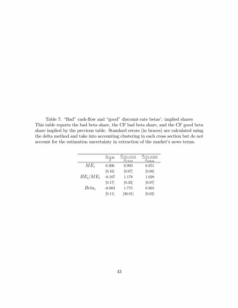
Table 7: �Bad� cash-ßow and �good� discount-rate betas�: implied sharesThis table reports the bad beta share, the CF bad beta share, and the CF good betashare implied by the previous table. Standard errors (in braces) are calculated usingthe delta method and take into accounting clustering in each cross section but do notaccount for the estimation uncertainty in extraction of the market�s news terms.

βCFMβ

βCFi,CFMβCFM

βCFi,DRMβDRM

MEi 0.306 0.993 0.851

[0.16] [0.07] [0.08]

BEi/MEi -0.107 1.178 1.028

[0.17] [0.33] [0.07]

Betai -0.003 1.775 0.865

[0.11] [36.01] [0.02]

43

Table 8: �Bad� cash-ßow and �good� discount-rate betas: Þrm-level regressions,monthly covariancesThe table shows pooled-WLS parameter estimates of Þrm-level multiple regressionsannually forecasting the subsequent average monthly cross products (NDR,t+NCF,t+NDR,t−1+NCF,t−1)∗(Ri,t), (NCF,t+NCF,t−1)∗(Ri,t), and (NDR,t+NDR,t−1)∗(Ri,t). Themarket�s NDR and NCF are the monthly news terms from Campbell and Vuolteenaho(2004). All variables are market adjusted by removing the corresponding year-speciÞccross-section mean. Independent variables, described in the text, are scaled to haveunit variance. Regression coefficients are divided by the estimated market monthlyreturn variance. All t-statistics (in parentheses) and standard errors (in braces) takeinto accounting clustering in each cross section but do not account for the estimationuncertainty in extraction of the market�s news terms.

β βCFM βDRMβCFMβ

Betai 0.1212 (4.37) 0.0117 (1.85) 0.1095 (4.26) 0.10 [0.05]

σi(ri) 0.1207 (3.70) 0.0040 (0.46) 0.1167 (4.24) 0.03 [0.07]

βROAi -0.0060 (-0.32) 0.0036 (1.16) -0.0096 (-0.47) -0.60 [1.67]

σi(ROAi) 0.0579 (5.44) 0.0099 (2.82) 0.0479 (4.48) 0.17 [0.06]

ROAi -0.0316 (-1.90) -0.0216 (-3.95) -0.0100 (-0.51) 0.68 [0.46]

Debti/Ai 0.0197 (1.63) 0.0073 (2.03) 0.0125 (1.17) 0.37 [0.20]

CAPXi/Ai -0.0154 (-1.89) -0.0060 (-2.00) -0.0095 (-1.36) 0.39 [0.19]

3.89% 0.60% 3.33%

44

Table 9: �Bad� cash-ßow and �good� discount-rate betas: Þrm-level tests, annualreturnsThe table shows pooled-WLS parameter estimates of Þrm-level multiple regressionsforecasting the annual cross products (NDR+NCF )∗(NCF,i+NDR,i), (NCF )∗(NCF,i+NDR,i), (NDR) ∗ (NCF,i +NDR,i), (NCF ) ∗ (NCF,i), (NDR) ∗ (NCF,i), (NCF ) ∗ (NDR,i),(NDR) ∗ (NDR,i). The market�s NDR and NCF are extracted using the VAR of Table1. All variables are market adjusted by removing the corresponding year-speciÞccross-section mean. Independent variables, described in the text, are normalized tohave unit variance. Regression coefficients are scaled by an estimate of the market�svariance. All t-statistics (in parentheses) take into accounting clustering in each crosssection but do not account for the estimation uncertainty in extraction of the market�snews terms.

β βCFM βDRM βCFi,CFM βCFi,DRM βDRi,CFM βDRi,DRMBetai 0.092 -0.002 0.093 -0.002 0.078 0.001 0.015

(3.05) (-0.21) (3.23) (-0.30) (3.17) (0.42) (2.67)

σi(ri) 0.090 0.012 0.077 0.011 0.075 0.001 0.003

(1.45) (1.27) (1.39) (1.25) (1.41) (0.79) (0.67)

BetaROAi 0.003 -0.002 0.005 0.000 0.014 -0.002 -0.009

(0.10) (-0.57) (0.20) (-0.08) (0.64) (-1.72) (-1.35)

σi(ROAi) 0.045 0.003 0.042 0.004 0.041 -0.002 0.002

(2.20) (0.35) (2.22) (0.58) (2.21) (-1.99) (0.69)

ROAi 0.021 0.011 0.009 0.016 0.011 -0.004 -0.002

(1.02) (1.69) (0.55) (2.18) (0.61) (-1.52) (-0.19)

Debti/Ai 0.015 0.007 0.008 0.005 0.007 0.002 0.001

(0.70) (1.18) (0.43) (0.82) (0.39) (1.79) (0.25)

CAPXi/Ai -0.009 -0.001 -0.009 -0.001 -0.008 0.000 0.000

(-0.48) (-0.16) (-0.47) (-0.28) (-0.49) (0.92) (-0.21)

1.36% 0.21% 1.22% 0.27% 1.18% 0.21% 0.60%

45

Table 10: �Bad� cash-ßow and �good� discount-rate betas: Þrm-level testsThis table reports the bad beta share, the CF bad beta share, and the CF good betashare implied by the multiple regressions in the previous table. Standard errors (inbraces) are calculated using the delta method and take into accounting clustering ineach cross section but do not account for the estimation uncertainty in extraction ofthe market�s news terms.

βCFMβ

βCFi,CFMβCFM

βCFi,DRMβDRM

Betai -0.020 1.277 0.840

[0.10] [1.88] [0.04]

σi(ri) 0.135 0.927 0.964

[0.08] [0.08] [0.04]

BetaROAi -0.859 0.148 2.584

[9.31] [1.49] [8.78]

σi(ROAi) 0.060 1.574 0.961

[0.16] [1.80] [0.05]

ROAi 0.549 1.372 1.161

[0.42] [0.34] [0.91]

Debti/Ai 0.488 0.663 0.889

[0.54] [0.29] [0.46]

CAPXi/Ai 0.080 1.643 0.950

[0.47] [4.59] [0.17]

46

1930 1940 1950 1960 1970 1980 1990 2000

-3

-2

-1

0

1

2

Figure 1: The Þgure plots three-year centered moving averages of −NM,DR (line withsquares) and NM,CF (thick solid line). The news terms are extracted from the VARmodel of Table 1. Both moving-average series are normalized to have a unit standarddeviation.

47