GROWTH MIRACLES REEXAMINED*

Chris Papageorgiou and Fidel P¶erez-Sebasti¶an**

WP-AD 2001-03

Correspondence to: Fidel P¶erez-Sebasti¶an, Dpto. Fundamentos de An¶alisis Econ¶omico, Universidad de

Alicante, Campus de San Vicente del Raspeig, 03071 Alicante, Spain, e-mail: ¯del@merlin.fae.ua.es

Editor: Instituto Valenciano de Investigaciones Econ¶omicas, S.A.

First Edition March 2001.

Dep¶osito Legal: V-893-2001

IVIE working papers o®er in advance the results of economic research under way in order to encourage

a discussion process before sending them to scienti¯c journals for their ¯nal publication.

* We thank Craig Burnside, John Du®y, Jordi Caballe, Theo Eicher, Lutz Hendricks, Pete Klenow, John Williams

and an anonymous referee for their comments and suggestions. We are especially grateful to Kazuo Mino whose input

greatly improved the paper. We also thank seminar participants at the Society of Computational Economics meetings,

University of Pompeu Fabra, Barcelona, 2000, the Midwest Macro meetings, University of Iowa, Iowa City, 2000,

the International Conference in Economic Growth, Acadimia Senica, Taipei, 1999, the 69th Southern Economic

Association meetings, New Orleans, 1999, the Symposium in Economic Analysis, Barcelona, 1999, the LSU seminar

series, 1999, and the Kumamoto Gakuen University seminar series, 1999, for their valuable comments. All remaining

errors are our own.

** C. Papageorgiou: LouIsiana State University; F. Perez-Sebastian: University of Alicante.

1

GROWTH MIRACLES REEXAMINED

Chris Papageorgiou and Fidel P¶erez-Sebasti¶an

A B S T R A C T

In this paper we propose a growth model in which the combined e®ect of human capital andtechnology adoption is the key factor in replicating and explaining growth miracles. Using standardtechnologies and parameterization, we show that the calibrated model generates output growthpaths consistent with the ones displayed by miracle economies, such as Japan and South Korea.The driving force of our result is twofold: (a) the complementarity between human capital andtechnological adoption; (b) the reallocation of labor across sectors along the adjustment path.

KEYWORDS: Transitional Dynamics; R&D; Input Complementarity.

2

1 INTRODUCTION

One of the most intriguing phenomena in modern economic growth is development miracles. The

stylized facts concerning fast growing economies are staggering. For example, over the period

1960¡1990, Japan and South Korea averaged output growth rates over 5 percent per year. During

this period, Japan's relative output per worker nearly tripled increasing from 20:6 to 60:3 percent

of the U.S. level, whereas S. Korean relative output per worker almost quadrupled increasing from

11:1 to 42:2 percent. Figure 1 illustrates the growth experiences of these two miracle countries.1

Closer observation of ¯gure 1 reveals an interesting feature of miraculous experiences: the sharp

increase of output per worker was characterized by growth rates that did not pick at the beginning

of the convergence process but later on, thus giving way to a hump-shaped growth path.

Figure 1: Output per worker growth rates in Japan and S. Korea, annual data, percentage

Japan

0

1

2

3

4

5

6

7

8

9

10

1950 1955 1960 1965 1970 1975 1980 1985 1990

S o u th K o re a

0

1

2

3

4

5

6

7

8

9

1 0

1 9 5 0 1 9 5 5 1 9 6 0 1 9 6 5 1 9 7 0 1 9 7 5 1 9 8 0 1 9 8 5 1 9 9 0

What is even more interesting is that the underlying characteristics of the two East Asian

miracle economies are distinctly di®erent. Whereas Japan started its post-War convergence path

with high human capital levels, S. Korea started its convergence path with very low human capital

levels. In addition, although both nations began with relatively low levels of physical capital,

Japan accumulated equipment, machinery, and infrastructure at a higher rate than S. Korea.2

Even regarding output growth rates, miraculous experiences show important di®erences. In ¯gure

1, we see that Japanese growth rates were relatively high from the beginning of the convergence

process, whereas S. Korean growth rates started low and increased rapidly.

1All along the paper, we follow Parente and Prescott (1994) and smooth the data series using the Hodrick-Prescott¯lter with the smoothing parameter equal to 25.

2The data that support these arguments are presented in section 4.4 of the paper.

3

The in°uential paper by Robert Lucas \Making a Miracle" concluded that improving our under-

standing of the mechanics of rapid growth episodes is essential in constructing a successful theory of

economic development. Since Lucas (1993), there has been surging interest in theoretical research

attempting to explain economic miracles, with a number of papers being able to reproduce the

average convergence speed exhibited by rapidly growing nations. However, as section 2 discusses

in more detail, growth models have not in general been able to predict the variable convergence

speed needed to generate the observed hump-shaped adjustment path of output growth rate. Nor

has the literature paid close attention to the distinct characteristics of miraculous episodes.

In this paper, we propose a model in which the complementarity between human capital and

technology adoption is able to replicate and explain growth miracles. As Parente and Prescott

(1994), we focus on di®erences in barriers to technology adoption. Parente and Prescott (1994)

replicate the average speed of convergence implied by the Japanese and S. Korean experiences;

variable convergence speeds are also possible in their model but only through exogenous variations

in the degree of barriers. Whereas in Parente and Prescott's work technology barriers are exogenous

and an increasing function of sociopolitical factors such as corruption, legal constraints and violence,

in our paper they are endogenously determined and depend on the level of human capital.3

More precisely, we introduce endogenous human capital accumulation into an, otherwise, styl-

ized R&D-based growth model. We use a version of Jones (1995) hybrid non-scale growth framework

in which sustained long-run growth depends on both exogenous labor growth and endogenous tech-

nical change.4 In our model, technical progress is enhanced through innovation and imitation,

and human capital through formal schooling. Even though formal schooling is not the only source

of human capital, we choose a schooling-based human capital technology because the model will

ultimately be taken to the data, and by many accounts the best available data used to measure

human capital across countries are the educational attainment data sets of Barro and Lee (1993)

and Nehru, Swanson, and Dubey (1995). Our choice of schooling technology follows the Mincerian

approach (Mincer 1974) that has recently been revived by Bils and Klenow (forthcoming).5

3Our model is also consistent with Griliches (1988a) and Nelson and Pack (1999), who emphasize the need ofaccumulating enough skills before being able to use new techniques and manufacture new products.

4Other growth models that eliminate scale e®ects include Sergerstrom (1998), Eicher and Turnovsky (1999), Young(1998), Dinopoulos and Thompson (1998), and Howitt (1999). The last three of these papers also permit sustainedoutput growth in the absence of population growth. We choose Jones' technology speci¯cation because it lends itselfmore easily to our numerical analysis.

5For recent discussions on the advantages of the Mincerian approach in growth modeling and estimation, see Bilsand Klenow (forthcoming), and Krueger and Lindahl (1998). Other papers that employ the Mincerian approach to

4

We then use numerical-approximation techniques based on Judd (1992) to simulate the tran-

sitional dynamics of the model, and compare their predictions to the data. Using standard tech-

nologies and parameterization, we show that the calibrated model can successfully replicate the

growth experiences of Japan and S. Korea. The key factor contributing to this result is twofold:

(a) the complementarity between human capital and technological adoption, (b) the reallocation

of labor across sectors along the adjustment path. The model can also account for the di®erent

underlying characteristics of the Japanese and S. Korean experiences. First, we show that lower

schooling levels are associated with slower physical capital accumulation. A smaller human capital

stock implies a larger productivity of schooling time; thus reducing the amount of labor allocated

to ¯nal output production which in turn reduces physical capital formation. Second, we show that

output growth rates at the beginning of the convergence process increase with the average educa-

tional attainment. This is because the rates of technology adoption and physical capital formation

increase with human capital, causing output to accumulate at a faster rate.

There is a small but rapidly growing literature that investigates the relationship between human

capital accumulation and technological progress, and their combined e®ect on economic growth.

Eicher (1996) develops a model in which both human capital and technological innovation are

endogenous. Eicher, however, is only concerned with steady-state predictions. Restuccia (1997)

presents a dynamic general equilibrium model with schooling and technology adoption. But he

focuses on how schooling and technology adoption may be amplifying the e®ects of productiv-

ity/policy di®erences on income disparity. Lau and Wan (1994) also reproduce the growth patterns

shown by East Asian miracle countries in a model of human capital and technological catch-up, but

their model's setup is rather ad hoc. Like us, Funke and Strulik (2000) study transitional dynamics

in a model of physical capital, human capital, and blueprints. They, however, study the existence

of threshold levels in the parameters that switch on and o® the di®erent sectors.

The remainder of the paper is organized as follows. Section 2 presents a review of existing

models and their convergence implications. It also o®ers arguments in favor of a proposed model

that can reproduce miracles experiences. Section 3 presents the basic model. In this section, we

establish the economic environment and examine the steady-state properties of the model. The

transitional dynamics analysis is presented in Section 4. Section 5 concludes discussing the main

¯ndings of our work.

model schooling include Jones (1997, 1999), Jovanovic and Rob (1998), and Hall and Jones (1999).

5

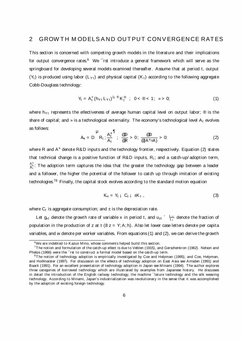
2 GROWTH MODELS AND OUTPUT CONVERGENCE RATES

This section is concerned with competing growth models in the literature and their implications

for output convergence rates.6 We ¯rst introduce a general framework which will serve as the

springboard for developing several models examined thereafter. Assume that at period t, output

(Yt) is produced using labor (LY t) and physical capital (Kt) according to the following aggregate

Cobb-Douglass technology:

Yt = A»t (hY t LY t)

1¡® K®t ; 0 < ® < 1 ; » > 0; (1)

where hY t represents the e®ectiveness of average human capital level on output labor; ® is the

share of capital; and » is a technological externality. The economy's technological level At evolves

as follows:

_At = D

µRt ;

A¤t

At

¶;

@D

@R> 0 ;

@D

@(A¤=A)> 0: (2)

where R and A¤ denote R&D inputs and the technology frontier, respectively. Equation (2) states

that technical change is a positive function of R&D inputs, Rt; and a catch-up/adoption term,

A¤t

At: The adoption term captures the idea that the greater the technology gap between a leader

and a follower, the higher the potential of the follower to catch up through imitation of existing

technologies.78 Finally, the capital stock evolves according to the standard motion equation

_Kt = Yt ¡ Ct ¡ ±Kt , (3)

where Ct is aggregate consumption; and ± is the depreciation rate.

Let gxt denote the growth rate of variable x in period t, and uzt ´ LztLt

denote the fraction of

population in the production of z at t (8 z = Y; A; h). Also let lower case letters denote per capita

variables, and w denote per worker variables. From equations (1) and (2), we can derive the growth

6We are indebted to Kazuo Mino, whose comments helped build this section.7The notion and formulation of the catch-up e®ect is due to Veblen (1915), and Gerschenkron (1962). Nelson and

Phelps (1966) were the ¯rst to construct a formal model based on the catch-up term.8The notion of technology adoption is empirically investigated by Coe and Helpman (1995), and Coe, Helpman,

and Ho®maister (1997). For discussion on the e®ects of technology adoption on East Asia see Amsden (1991) andBaark (1991). For an excellent presentation of technology adoption in Japan see Minami (1994). The author exploresthree categories of borrowed technology which are illustrated by examples from Japanese history. He discussesin detail the introduction of the English railway technology, the machine ¯lature technology and the silk weavingtechnology. According to Minami, Japan's industrialization was revolutionary in the sense that it was accomplishedby the adoption of existing foreign technology.

6

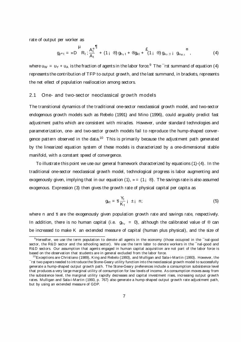
rate of output per worker as

gywt = » D

µRt ;

A¤t

At

¶+ (1 ¡ ®) ghY t + ®gkt +

£(1 ¡ ®) guY ;t ¡ guW;t

¤, (4)

where uW = uY +uA is the fraction of agents in the labor force.9 The ¯rst summand of equation (4)

represents the contribution of TFP to output growth, and the last summand, in brackets, represents

the net e®ect of population reallocation among sectors.

2.1 One- and two-sector neoclassical growth models

The transitional dynamics of the traditional one-sector neoclassical growth model, and two-sector

endogenous growth models such as Rebelo (1991) and Mino (1996), could arguably predict fast

adjustment paths which are consistent with miracles. However, under standard technologies and

parameterization, one- and two-sector growth models fail to reproduce the hump-shaped conver-

gence pattern observed in the data.10 This is primarily because the adjustment path generated

by the linearized equation system of these models is characterized by a one-dimensional stable

manifold, with a constant speed of convergence.

To illustrate this point we use our general framework characterized by equations (1)-(4). In the

traditional one-sector neoclassical growth model, technological progress is labor augmenting and

exogenously given, implying that in our equation (1), » = (1¡®). The savings rate is also assumed

exogenous. Expression (3) then gives the growth rate of physical capital per capita as

gkt = sYt

Kt¡ ± ¡ n; (5)

where n and s are the exogenously given population growth rate and savings rate, respectively.

In addition, there is no human capital (i.e. ghY= 0), although the calibrated value of ® can

be increased to make K an extended measure of capital (human plus physical), and the size of

9Hereafter, we use the term population to denote all agents in the economy (those occupied in the ¯nal-goodsector, the R&D sector and the schooling sector). We use the term labor to denote workers in the ¯nal-good andR&D sectors. Our assumption that agents engaged in human capital acquisition are not part of the labor force isbased on the observation that students are in general excluded from the labor force.

10Exceptions are Christiano (1989), King and Rebelo (1993), and Mulligan and Sala-i-Martin (1993). However, the¯rst two papers needed to introduce the Stone-Geary utility function into the neoclassical growth model to successfullygenerate a hump-shaped output growth path. The Stone-Geary preferences include a consumption subsistence levelthat produces a very large marginal utility of consumption for low levels of income. As consumption moves away fromthe subsistence level, the marginal utility rapidly decreases and capital investment rises, increasing output growthrates. Mulligan and Sala-i-Martin (1993, p. 767) also generate a hump-shaped output growth rate adjustment path,but by using an extended measure of GDP.

7

population equals the labor force (i.e. guW ;t = 0). Hence, equation (4) becomes

gywt = gyt = (1 ¡ ®) ¹gA + ®

µs

Yt

Kt¡ ± ¡ n

¶; (6)

where ¹gA denotes an exogenous rate of technological progress.

Given that less developed countries generally possess small output to capital ratios, the neoclas-

sical framework predicts that the convergence process of these economies will be characterized by

an initial growth rate of output larger than its steady-state value. Moreover, YK will converge mono-

tonically due to diminishing marginal returns to capital, thus making output display monotonically

decreasing growth rates.11

In two-sector endogenous growth models, technology is assumed to be a constant parameter

and therefore ¹gA equals zero. For economically meaningful parameter values, Mulligan and Sala-i-

Martin (1993) show that the growth rates of physical capital and human capital are inverse functions

of their relative stocks. Given that these models carry out their analyses in per capita terms, and

that gyt = gywt ¡ guW t, we can now write equation (4) as

gyt = (1 ¡ ®)

·gh

µhY t

kt

¶+ guY

¸+ ® gk

µkt

hY t

¶: (7)

It turns out that the decline of growth rate of the relatively scarce capital is faster than the increase

in growth rate of the abundant capital. As a result, a decreasing pattern characterizes most of the

adjustment path of output per capita growth.

2.2 R&D-based growth model

A variable speed of convergence is crucial if we want growth rates not to pick at the beginning

of the adjustment path. Eicher and Turnovsky (1999) ¯nd that variable convergence speed is

possible in non-scale versions of growth models of physical capital accumulation and technical

change. The di®erence from the endogenous two-sector growth models is the °exibility in returns

to scale permitted by the non-scale production function. In addition, Perez-Sebastian (2000) shows

that the introduction of technology imitation in non-scale models of growth is critical in replicating

growth miracles. Technology adoption fuelled by cheap imitation is shown to also be the key in

Parente and Prescott (1994). Growth rates in these models, however, still pick at the beginning of

the adjustment path because of the large productivity of imitation.

11This conclusion does not change when the saving rate is determined by the optimal choice of consumption overtime (see, for instance, King and Rebelo (1993)).

8

Equation (2) implies that, when technical progress becomes endogenous, the rate at which

technology is acquired depends both on R and¡

A¤A

¢. The latter contributes to generate a larger

convergence rate at early stages of development because the technological gap is then relatively

larger. The former, however, can do the opposite because R&D inputs may rise with the level of

the state variables. Which one dominates will depend on the technology used to produce R. Parente

and Prescott (1994) and Perez-Sebastian (2000) present similar technology adoption structures as

the one of equation (2). In the former, R takes the form of physical capital, whereas in the latter

R is produced with the same technology as output. Even though both models have contributed

in our understanding of development miracles, neither model induces a fast enough growth on R

to revert the declining convergence rate of output. Put di®erently, in both models the technology

catch-up engine is the dominating force of economic growth.

2.3 Adding human capital in R&D-based growth model

When R takes the form of either capital or output, one important limitation is that ¯nal output

leads and R follows; that is, Y must grow fast before R. This is actually the opposite scenario to

the one which we want to reproduce. Introducing human capital in R&D inputs can potentially

solve this problem { notice that the amount of human capital can grow fast independently of

output. Additionally, the endogenous determination of human capital creates a new sector that

can contribute to generate larger reallocations of population, thus inducing more variability in the

output growth rate (recall equation (4)).

In summary, the main argument of the analysis above is that neither the neoclassical growth

model nor the existing R&D-based growth models have been, in general, able to reproduce the

convergence path of development miracles. It is our conjecture that a model in which human

capital and technological progress are complementary engines of growth will be more successful in

reproducing miracles.

3 THE BASIC MODEL

In what follows, we propose an alternative model of economic growth with endogenous technological

change and human capital. We assign explicit forms to the implicit functions sketched in the

previous section, and embed them into a fully speci¯ed optimizing framework.

9

3.1 Economic environment

The population in this economy consists of identical in¯nitely-lived agents, and grows exogenously

at rate n: Agents are involved in three types of activities: consumption-goods production, R&D

e®ort, and human capital attainment.12 Each period, consumers are endowed with one unit of

time that is allocated between working and studying. We abstract from labor/leisure decisions and

assume that agents have preferences only over consumption.

Consumption goods are produced using the aggregate Cobb-Douglass production function given

by equation (1). R&D activity is the source of technological progress in the model. The R&D

technology is an explicit form of equation (2) as follows:

At+1 ¡ At = ¹AÁt (hAtLAt)

¸

µA¤

t

At

¶Ã

; Á < 1; 0 < ¸ · 1; Ã ¸ 0; A¤t ¸ At; (8)

where LAt is labor employed in the R&D sector at time t; hAt is a measure of e®ectiveness of

average skill level on labor employed in the R&D sector; Á represents a positive externality due to

the stock of existing technology; ¸ introduces diminishing returns to e®ective R&D labor; and à is

a technology gap parameter. We assume that the worldwide stock of existing technology A¤t grows

exogenously at rate gA¤ .

Agents increase their human capital level through formal education, provided by a schooling

sector. The human capital technology is of particular interest in our model and deserves careful

consideration. Since our aim is to take the model to the data then our speci¯cation ought to be one

that maps the available data on average years of education to the stock of human capital. Using

the Mincerian interpretation seems to deliver such a speci¯cation. This representation follows Bils

and Klenow (forthcoming), who suggest that the Mincerian speci¯cation of human capital is the

appropriate way to incorporate years of schooling in the aggregate production function. Following

their approach, human capital per capita is given by

hjt = efj(St) ; j 2 fY; Ag , (9)

where St is the population average years of schooling at date t.13 The derivative f 0j (St) represents

12Schooling is assumed to be the only source of human capital attainment in this model. Allowing for other typesof human capital attainment such as learning-by-doing, studied by Stokey (1988) and Lucas (1993), would be aninteresting extension of the model and worthy of future research.

13Our baseline assumption is that human capital augments labor productivity in R&D di®erently than laborproductivity in output (i.e. fA(S) 6= fY (S)). In our calibration exercises, we also examine the case where humancapital e®ectiveness is the same on all productive labor (i.e. fA(S) = fY (S) = f(S)).

10

the return to schooling estimated in a Mincerian wage regression in sector j: an additional year of

schooling raises a worker's e±ciency by f 0j (St).

14

Next, we are concerned with the behavior of St. In particular, we derive a law of motion of

St that is consistent with the following two desirable properties: (a) the evolution of St depends

on the share of people in education, (b) in steady state, St is constant. As it is counter-factual to

assume that St grows inde¯nitely, the second property indicates that at steady state the average

years of education reaches a ¯xed number.15

We assume that, each period, agents allocate time to human capital formation only after output

production has taken place. Let LHt be the total amount of people that attend school in the

economy at date t. Assume that at some point in time, say period 1, the average educational

attainment equals zero. Next period, given that consumers live for ever, the average years of

schooling will be S2 = LH1L2

, where Lt is the population size at date t. In period 3, S3 = LH1+LH2L3

,

and so on. Hence, the average educational attainment can be written as

St =

Pt¡1j=1 LHj

Lt. (10)

From equation (10), we can derive the law of motion of the average educational attainment as

follows:

St+1 ¡ St =

Ptj=1 LHj

Lt+1¡

Pt¡1j=1 LHj

Lt;

=

µ1

1 + n

¶ µLHt

Lt¡ n St

¶: (11)

Notice that the above motion equation has the two desirable properties mentioned above: the

evolution of St depends on the share of people in education, LHL , and average years of schooling

at steady state, Sss; reaches an upper bound remaining constant thereafter. The second property

holds because, as will be clear later, the ratio LHL is invariant at steady state; dividing expression

(11) by St, we can then easily see that variable S can grow at a constant rate only if S is a constant.

14Mincer (1974) estimates the following wage regression equation:

!i = ¯0 + ¯1(SCH)i + ¯2(EXP )i + ¯3(EXP )2i + "i;

where !i is the log wage for individual i, SCH is the number of years in school, EXP is the number of years of workexperience, and " is a random disturbance term.

15For further discussion on this issue see Jones (1996, 1997).

11

3.2 Social planner's problem

For simplicity of exposition, we focus on a centrally planned economy.16 A central planner inter-

nalizes the externalities and chooses the sequences fCt, St; At, Kt, LY t, LAt, LHtg1t=0 so as to

maximize the lifetime utility of the representative consumer subject to the feasibility constraints of

the economy, and the initial values L0; S0; K0; and A0. The problem is stated as follows:

maxfCt;St;At;Kt;LY t;LAt;LHtg

1Xt=0

½t

264³

CtLt

´1¡µ ¡ 1

1 ¡ µ

375 ; (12)

subject to,

Yt = A»t

hefY (St)LY t

i1¡®K®

t ; (13)

It = Kt+1 ¡ (1 ¡ ±) Kt = Yt ¡ Ct; (14)

At+1 ¡ At = ¹AÁt

hefA(St)LAt

i¸µ

A¤t

At

¶Ã

; (15)

St+1 ¡ St =

µ1

1 + n

¶ µLHt

Lt¡ n St

¶; (16)

Lt = LY t + LAt + LHt; (17)

Lt+1

Lt= 1 + n; for all t; (18)

A¤t+1

A¤t

= 1 + gA¤ ; (19)

L0; S0; K0; A0 given,

where µ is the inverse of the intertemporal elasticity of substitution; and ½ is the discount factor.

Equation (14) is the economy's feasibility constraint as well as the law of motion of the stock of

physical capital; it says that, at the aggregate level, domestic output must equal consumption plus

physical capital investment, It. Equation (17) is the population constraint; the labor force { the

number of people employed in the output and the R&D sectors { plus the number of individuals

going to school must be equal to the population.

16It is well known that in models with externalities like ours, appropriate policies by the social planner can achievethe ¯rst best. We assume that these policies are imposed in our economy and focus on the social planner's problem.

12

The optimal control problem can be stated as follows:

V (At; Kt; St) = maxfLHt;LAt;Itg

·A»

t [efY (St)(Lt¡LHt¡LAt)]1¡®K®t ¡ It

Lt

¸1¡µ

¡ 1

1 ¡ µ+

+½ V

"At + ¹AÁ

t

³efA(St)LAt

´¸µ

A¤t

At

¶Ã

; Kt(1 ¡ ±) + It ; St +1

1 + n

µLHt

Lt¡ nSt

¶#; (20)

where V (¢) is a value function; LHt; LAt; It are the control variables; and At; Kt; St are the

state variables. Solving the optimal control problem gives the Euler equations that characterize

the optimal allocation of population in human capital investment, in R&D investment, and in

consumption/physical capital investment respectively as follows:µCt

Lt

¶¡µ (1 ¡ ®)Yt

LY t=

½

1 + n

µCt+1

Lt+1

¶¡µ (1 ¡ ®)Yt+1

LY;t+1

·1 + f 0

Y (St+1)LY;t+1

Lt+1+ f 0

A(St+1)LA;t+1

Lt+1

¸;

(21)µCt

Lt

¶¡µ (1 ¡ ®)Yt

LY t=

½

1 + n

µCt+1

Lt+1

¶¡µ ¸ (At+1 ¡ At)

LAt¤

¤8<:»Yt+1

At+1+

·1 + (Á ¡ Ã)

µAt+2 ¡ At+1

At+1

¶¸ 24 (1¡®)Yt+1

LY;t+1

¸(At+2¡At+1)LA;t+1

359=; ; (22)

µCt

Lt

¶¡µ

=½

1 + n

µCt+1

Lt+1

¶¡µ ·®Yt+1

Kt+1+ (1 ¡ ±)

¸: (23)

At the optimum, the planner must be indi®erent between investing one additional person in

schooling, R&D, and ¯nal output production. The LHS of equations (21) and (22) represent the

return from allocating one additional unit of labor to output production. The RHS of equation (21)

is the discounted marginal return to schooling, taking into account population growth. The RHS

term in brackets arises because human capital determines the e®ectiveness of labor employed in

output production as well as in R&D. The RHS of equation (22) is the return to R&D investment.

An additional unit of R&D labor generates ¸(At+1¡At)LAt

new ideas for new types of producer durables.

Every new design increases next period's output by »Yt+1

At+1and R&D production by dAt+2

dAt+1times

(1¡®)Yt+1

LY;t+1

h¸(At+2¡At+1)

LA;t+1

i¡1; where (1¡®)Yt+1

LY;t+1

h¸(At+2¡At+1)

LA;t+1

i¡1gives the value of one additional design

that equalizes labor wages across sectors. Euler equation (23) is standard. It says that the planner

is indi®erent between consuming one additional unit of output today and converting it into capital,

thus consuming the proceeds tomorrow.

13

3.3 Steady-state growth

We now derive the model's balanced-growth path. Solving for the interior solution, equation (17)

implies that in order for the labor allocations to grow at constant rates, LHt, LY t and LAt must

all increase at the same rate as Lt. This means that the ratio LHtLt

is invariant along the balanced-

growth path. Hence, equation (16) implies that, at steady-state (ss), Sss is constant and equals

Sss =uh;ss

n; (24)

where uh;ss = LHL

¯ss

: Equation (24) shows that along the balanced growth path, the economy

invests in human capital just to provide new generations with the steady-state level of schooling.

This is consistent with work by Jones (1996, 1997), where growth regressions are developed from

steady-state predictions, and data on Sss acts as a proxy for uh;ss; the estimated coe±cient on Sss

in part re°ects the parameter 1n in our framework.

Let Gxt = 1 + gxt: The aggregate production function, given by equation (13), combined with

the steady-state condition gY;ss = gK;ss delivers the gross growth rate of output as a function of

the gross growth rate of technology as

GY;ss = (GA;ss)»

1¡® (1 + n) : (25)

Since GA;ss is constant, it follows from equation (8) that

GA;ss =h(1 + n)¸GÃ

A¤;ss

i 11+áÁ

: (26)

Equation (26) shows the relationship between the technology frontier growth rate and the tech-

nology growth rate of the model economy. Figure 1 illustrates this relationship.Notice that since

the ratio Ã1+áÁ < 1, the function is concave with a unique point at which GA;ss equals GA¤;ss; in

particular,

GA;ss = GA¤;ss = (1 + n)¸

1¡Á : (27)

The gross rate GA;ss cannot be larger than GA¤;ss otherwise At will eventually become bigger

than A¤t , and this has been ruled out by assumption. But GA;ss can be smaller than GA¤;ss. For

simplicity, we focus on the special case in which all countries grow at the same rate at steady state;

14

Figure 2: Relationship between GA;ss and GA¤;ss

GA

GA < GA*GA > GA*

45o

GA = GA*

that is, we assume that GA¤;ss is given by expression (27), and therefore so is GA;ss.17 This in turn

implies that

GY;ss = GC;ss = GK;ss = (1 + n)¸»

(1¡®)(1¡Á) : (28)

Consistent with Jones (1995) our balanced-growth path is free of \scale e®ects", and policy has no

e®ect on long-run growth. The reason why our model's long-run growth is equivalent to that of

Jones even in the presence of a schooling sector, is that at steady state the mean years of education,

St; reaches a constant level Sss.

3.4 Population shares in output, R&D, and schooling

Next, we derive the steady-state shares of labor in the three sectors of the economy. Euler equation

(21) combined with the balanced-growth equation (28) gives

Gµ¡1y;ss (1 + n)

½¡ 1 = f 0

Y (Sss) uY;ss + f 0A(Sss) uA;ss; (29)

17Alternatively, we could assume that a leading economy that is at steady-state is the one that moves the worldtechnological frontier according to equation (8) which now reduces to

A¤t+1 ¡ A¤

t = ¹A¤Át (h¤

AtL¤At)

¸;

where ¤ denotes the value on which variables take in the leading country. Notice that nowA¤

tAt

= 1 because imitation

is not possible at the frontier. In such case G¤A = 1 + g¤

A = (1 + n¤)¸

1¡Á as in Jones (1995). Assuming that n = n¤,and substituting G¤

A into equation (26) delivers equation (27). As discuss in footnote 18, had g¤A taken on any other

value, the transitional dynamics numerical analysis would become much more tedious.

15

where uY;ss = LYL

¯ss

and uA;ss = LAL

¯ss

: The steady-state shares of R&D and output-production

labor are inversely related to the return to education, other things constant.

Euler equation (22) combined with balanced-growth condition (28) deliver the steady-state

labor share in R&D as

uA;ss =uY;ss³

1¡®¸»gA;ss

´ hGµ¡1

y;ss

³GA;ss

½

´¡ (Á ¡ Ã)gA;ss ¡ 1

i : (30)

Equations (29) and (30), and the population constraint

uY;ss = 1 ¡ uh;ss ¡ uA;ss; (31)

give the three steady-state equilibrium shares of labor.

4 TRANSITIONAL DYNAMICS

This section is concerned with the transitional dynamics of the model economy. Since there is

no analytical solution to our system we use numerical approximation techniques to simulate the

transitional dynamics of the model, and then take their predictions to the data.

4.1 The normalized system

We start by rede¯ning variables so that they take constant values along the balanced-growth path.

The aggregate production function, equation (13), suggests that we normalize variables by the

term A»

1¡®t Lt. We can then rewrite consumption, physical capital and output as ct = Ct

A»

1¡®t Lt

,

kt = Kt

A»

1¡®t Lt

and yt = Yt

A»

1¡®t Lt

, respectively. Using equation (21) gives

µct+1

ct

¶µ µuY;t+1

uY t

¶(GAt)

(µ¡1)»1¡®

µyt

yt+1

¶=

µ½

1 + n

¶ £f 0

Y (St+1) uY;t+1 + f 0A(St+1) uA;t+1 + 1

¤: (32)

From the R&D equation (8), we derive GAt as

GAt =At+1

At= 1 + À

hefA(St)uAt

i¸T (1+áÁ); (33)

where T =A¤

tAt

; and À = ¹ (A¤t )Á¡1 L¸

t , which is a constant.18 From equation (22) we get

18To show that À is constant requires some algebra. Rewriting the equality in its gross growth form,Àt+1

Àt=

GÁ¡1A¤t (1 + n)¸; and given that GA¤t = GA;ss = (1 + n)

¸1¡Á ; it follows that

Àt+1

Àt= 1. Notice that if A¤

t did not grow

according to equation (27), À could not be constant, making the simulation exercise more tedious.

16

µct+1

ct

¶µ µyt

yt+1

¶ µuY;t+1

uY t

¶=

½ gAt

G»

1¡®(µ¡1)+1

At

µuA;t+1

uAt

¶¤

¤·µ

¸»

1 ¡ ®

¶ µuY;t+1

uA;t+1

¶+

µ1

gA;t+1

¶+ (Á ¡ Ã)

¸: (34)

Finally, from equation (23) we obtain

1 + n

½

·µct+1

ct

¶(GAt)

»1¡®

¸µ

= ®yt+1

kt+1

+ (1 ¡ ±): (35)

The system that determines the dynamic equilibrium normalized allocations are formed by the

conditions associated with three control and three state variables as follows:

Control Variables:

1. Euler equation for population share in schooling, uht: Eq. (32).

2. Euler equation for population share in R&D, uAt: Eq. (34).

3. Euler equation for normalized consumption, ct: Eq. (35).

Subject to the population constraint uY t = 1 ¡ uAt ¡ uht:

State Variables:

1. Law of motion of human capital, St: Eq. (11).

2. Law of motion of technology, At: Eq. (33).

3. Law of motion of normalized physical capital, kt:

(1 + n)kt+1 (GAt)»

1¡® = (1 ¡ ±)kt + yt ¡ ct; (36)

where

Tt+1 = Tt

µGA¤t

GAt

¶; (37)

and

yt = k®t

hefY (St) uY t

i1¡®: (38)

To solve the above system of dynamic equations, we follow Judd (1992), approximating the

policy functions employing high-degree polynomials in the state variables.19

19In particular, the parameters of the approximated decision rules are chosen to (approximately) satisfy the Eulerequations over a number of points in the state space, using a nonlinear equation solver. A Chebyshev polynomial

17

Table 1: Parameter values used in the simulations

® 0.36 » 0.1 Sss 12.5

½ 0.96 Gy 1.016 ´ 0.69

± 0.06 ¸ 0.5 ¯ 0.43

n 0.0116 Á 0.94 µ 1.28

4.2 Calibration

Table 1 shows the parameter values used to carry out the simulations. We choose a value of 0:06

for the depreciation rate (±), and a value of 1:016 for the steady-state gross growth rate of income

(Gy;ss), the average number in the Bils and Klenow's (forthcoming) 91-country sample. We assign

values of 0:36 to the capital-share of output (®), and 0:96 to the discount factor (½). We set the

population growth rate (n) to 0:0116 per year, which is the average growth rate of the labor force

in the G-5 countries (France, West Germany, Japan, the United Kingdom, and the United States)

during the period 1965-1990. Regarding the value of the elasticity of output with respect to the

technology, Griliches (1988b) reports estimates of » between 0:06 and 0:1. Following Eicher and

Turnovsky (1999), we choose » = 0:1.

It is not clear what the steady-state value of the average educational attainment ought to be,

given that mean years of schooling have been increasing over the last decades in most developed

countries. We choose to set Sss to 12:5, to match the 1993 U.S. ¯gure. To estimate the human

capital equations, we ¯rst assume that

fY (S) = fA(S) = f(S) = ´S¯, ´ > 0; ¯ > 0: (39)

Following Bils and Klenow (forthcoming), we use Psacharopoulos' (1994) cross-country sample on

average educational attainment and Mincerian coe±cients to estimate ´ and ¯. Given equation

(39), we can construct the regression equation

ln (Minceri) = a + b ln Si + "i; (40)

basis is used to construct the policy functions, and the zeros of the basis form the points at which the system issolved; that is, we use the method of orthogonal collocation to choose these points. Finally, tensor products of thestate variables are employed in the polynomial representations. This method has proven to be highly e±cient insimilar contexts. For example, for the one-sector growth model, Judd (1992) ¯nds that the approximated values ofthe control variables disagree with the values delivered by the true policy functions by no more than one part in10,000. All programs are written in GAUSS and are available by the authors upon request.

18

Table 2: The Japanese and Korean experiences

Country In 1960 In 1963 In 1990

Japan

Y per worker (%)

K per worker (%)

S (years)

TFP (uY = 1) per worker (%)

20:616:910:240:0

60:3104:611:0¤

59:5¤

S. Korea

Y per worker (%)

K per worker (%)

S (years)

TFP (uY = 1) per worker (%)

11:011:63:238:8

42:250:27:7¤

58:3¤¤ 1987 ¯gures.

where Minceri = f 0(Si) is the estimated Mincerian coe±cient for country i; a and b equal ln(´¯)

and (¯ ¡ 1) ; respectively; and "i is a random disturbance term. We obtain estimates of ´ = 0:69

and ¯ = 0:43 that are very similar to those obtained by Bils and Klenow (forthcoming).20 Equations

(24) and (29) imply that the inverse of the intertemporal elasticity of substitution (µ) must then

equal 1:28, which is well within the empirical estimates.

Estimates of ¸ found in the literature vary from 0:2 to 0:75, so we carry out a sensitivity analysis

with ¸ taking the values 0:25, 0:5, and 0:75. Since the results we obtain are almost identical, we

choose to use the intermediate value, ¸ = 0:5. From equation (27), we can then recover the value

of Á = 0:94. We choose à so as to reproduce the output per worker evolution between 1960 and

1990 in Japan, and between 1963 and 1990 in S. Korea.21 The former development experience

gives a value for à of 0:21, whereas the latter implies that à equals 0:26. The initial values of the

stock variables and output data used to calibrate à are presented in table 2; accuracy measures are

presented in table 3.

4.3 Asymptotic stability and asymptotic speed of convergence

As a crucial ¯rst step, we establish the asymptotic stability of our model's long-run equilibrium.

Linearizing the normalized system of equations around the steady state, we ¯nd that for any

reasonable parameter values, the transition is characterized by a three-dimensional stable saddle-

20Both estimates are signi¯cantly di®erent from zero at the 1 percent level.21Japan's rapid convergence toward U.S. income levels actually started right after WWII. Unfortunately, the

Japanese Education Department does not possess estimates of the average educational attainment before 1960. Weare grateful to Tomoya Sakagami who has attempted to obtain this data for us.

19

Table 3: Accuracy measures

Average Error (%)¤ Max. Error (%)¤

Country à C uY uA C uY uA

Japan 0:21 0:01 0:02 0:01 0:04 0:09 0:07S. Korea 0:26 0:08 0:23 0:09 0:35 1:16 0:45S. Korea 0:28 0:08 0:37 0:18 0:32 1:32 0:86¤ We assess the Euler equation error over 10,000 state-space points using the approximated rules. For

each variable, the measure gives the current value decision error that agents using the approximated

rules make, assuming that the (true) optimal decisions were made in the previous period.

path. The adjustment path is then asymptotically stable and unique; furthermore, growth rates

and convergence speeds can, as a consequence, vary across time and variables.

Next, we investigate the asymptotic speed of convergence { the rate by which a country's

output converges to its balanced growth path once the country is su±ciently close to its long-run

equilibrium. In our model, this speed is given by the largest eigenvalue among those contained in the

unit circle. The one sector neoclassical growth model implies convergence speed of about 7%, which

is inconsistent with most of the empirical evidence { Barro and Sala-i-Martin (1995) and Temple

(1998), among others, report convergence-speed estimates for OECD nations of approximately 2%.

Table 4 presents implied speeds for di®erent values of ¸ and Ã:

Table 4: Asymptotic speed of convergence for di®erent values of ¸ and Ã

¸Âà 0:20 0:24 0:28 0:30

0:25 1:43% 1:66% 1:93% 2:08%0:50 1:16% 1:32% 1:46% 1:52%0:75 1:06% 1:19% 1:31% 1:37%

Parameter values in the neighborhood of those employed in our calibration deliver speeds of

convergence that vary between 1:06%¡2:08%; consistent with most empirical evidence. In addition,

our results are consistent with the ¯nding of Eicher and Turnovsky (1999), that moving from one-

sector to multi-sector non-scale growth models with endogenous technological change leads to severe

reduction in the asymptotic speed of convergence.

20

4.4 Adjustment paths of Japan and S. Korea

We choose to calibrate à to both the S. Korean and the Japanese output paths because they

represent two very di®erent \miraculous" experiences. Table 2 presents data for S. Korea and

Japan on relative levels of GDP per worker (RGDPW), relative physical capital per worker, average

educational attainment, and relative TFP, which is broadly de¯ned and includes everything not

already captured by the other two stock variables (S and K).22 Between 1960 and 1990, Japan's

relative output per worker increased from 20:6 to 60:3 percent. GDP per worker in S. Korea started

its fast growing path around 1963; during the period 1963-1990, its relative level increased from

11:0 to 42:2 percent. During these periods, Japan and S. Korea exhibited, on average, a 5:2 and a

6:5 percent annual growth rates, respectively.

Japan had lost a substantial portion of its physical capital during WWII, but its educational

attainment in 1960 of 10:2 years compared well with those of the most developed nations { e.g., the

U.S. educational attainment at that time was a little over 10:7.23 What is even more interesting is

that during the period 1960-1987, average years of schooling of workers increased very little, only

by 0:8 years. The main engine of growth in Japan seems to have been physical capital accumulation

induced in part by a very important technological catch-up process. In 1960, the Japanese physical

capital stock per worker was only 16:9 percent; in 1990 reached a stunning 104:6 percent, which

implies an average annual convergence rate of 6:3 percent.

The S. Korean development experience, on the other hand, is distinctly di®erent from the

Japanese experience. As shown in table 2, even though output convergence was faster in S. Korea,

capital accumulated in this country at a lower rate than in Japan, growing from 11:6 to 50:2 percent

during the relevant period; that is an average annual convergence rate of 5:6 percent. It is human

capital accumulation that seems to have played the key role in S. Korean development process.

In particular, the average educational attainment more than doubled in the period 1963-1987,

increasing from 3:2 to 7:7 years.

Despite di®erent development experiences, both Japan and S. Korea obtain very close calibrated

values of Ã. The adjustment paths predicted by the model for the level and growth rates of relative

GDP per worker are depicted in ¯gure 3 and replicate fairly well the Japanese and the S. Korean

22All relative measures in the paper are with respect to U.S. levels.23Human capital levels in Japan were high before WWII. After the Meiji Restoration of 1868, one of the policy

priorities of the Meiji government was to introduce a nationwide education system under which all children from 6through 13 years of age were required to attend school (see Ozawa (1985)).

21

Figure 3: Adjustment paths for Japan and S. Korea

0

10

20

30

40

50

60

1950 1955 1960 1965 1970 1975 1980 1985 1990

Re

lati

ve

GD

PW

(%

)

Japanese Data

Predictions

(ψ = 0 .2 1 )

0

10

20

30

40

50

60

1960 1965 1970 1975 1980 1985 1990

Re

lati

ve

GD

PW

(%

)

Korean D ata

Pred ic tions

(ψ = 0 .2 6 )

0

2

4

6

8

10

12

14

1950 1955 1960 1965 1970 1975 1980 1985 1990

RG

DP

W g

row

th (

%)

Japanese Data

Predictions

(ψ = 0 .2 1 )

0

2

4

6

8

10

12

14

1960 1965 1970 1975 1980 1985 1990R

GD

PW

gro

wth

(%

) Korean Data

Predictions

(ψ = 0 .2 6 )

data. In particular, the model predicts that output per capita growth rates do not pick at the

beginning of the adjustment path but later on.

4.5 Discussion of the transition results

What are the determining factors behind our results? Figures 4 and 5 present the contributions of

di®erent components to S. Korean and Japanese output per worker growth, in line with equation (4).

The key force that generates the hump-shape is the relatively large allocation of agents in education

plus R&D activity at the beginning of the convergence process. To see this more clearly, recall that

the term in brackets in equation (4) re°ects the contribution of the movement of population across

sectors. More speci¯cally, this term takes into account that output growth rises with the amount

of labor devoted to ¯nal-good production, but also that additional labor force de°ates output per

worker. As a consequence, net labor contribution decreases with the number of students that leave

school { because the amount of workers then rise { and increases as R&D e®ort declines { because

part of the R&D labor is reallocated to the ¯nal output sector.

As shown in the bottom-right chart of ¯gures 4 and 5, the e®ect of students entering the labor

force is larger at the beginning, and rapidly decreasing as the economy approaches the steady

state, thus generating the fast declining pattern of labor force growth. This e®ect combined with a

22

Figure 4: Contribution of di®erent components to relative output growth, S. Korea

0

2

4

6

8

1 0

1 2

1 4

1 9 6 4 1 9 6 9 1 9 7 4 1 9 7 9 1 9 8 4 1 9 8 9

RG

DP

W g

row

th (

%

0

2

4

6

8

1 0

1 2

1 4

1 9 6 4 1 9 6 9 1 9 7 4 1 9 7 9 1 9 8 4 1 9 8 9

RT

FP

gro

wth

(%

-4

-2

0

2

4

6

8

1 0

1 9 6 4 1 9 6 9 1 9 7 4 1 9 7 9 1 9 8 4 1 9 8 9

Rk

gro

wth

(%

0

2

4

6

8

1 0

1 2

1 4

1 9 6 4 1 9 6 9 1 9 7 4 1 9 7 9 1 9 8 4 1 9 8 9

Rh

gro

wth

(%

-3

-1

1

3

5

7

9

1 1

1 9 6 4 1 9 6 9 1 9 7 4 1 9 7 9 1 9 8 4 1 9 8 9Ne

t la

bo

r c

on

trib

uti

on

0

2

4

6

8

1 0

1 2

1 4

1 9 6 4 1 9 6 9 1 9 7 4 1 9 7 9 1 9 8 4 1 9 8 9La

bo

r f.

sh

are

gro

wth

Black line: Model Predictions.

Grey line: Data.

Variables: RGDRW is relative GDP per worker; RTPF is relative TFP; Rk is relative

physical capital per capita; Rh is relative human capital per capita; Net labor contribution

represents the e®ect of the terms in brackets in equation (4); ¯nally, Labor f. share is labor force

share in the population.

23

Figure 5: Contribution of di®erent components to relative output growth, Japan

0

2

4

6

8

1 0

1 2

1 4

1 9 6 1 1 9 6 6 1 9 7 1 1 9 7 6 1 9 8 1 1 9 8 6

RG

DP

W g

row

th (

%

0

2

4

6

8

1 0

1 2

1 4

1 9 6 1 1 9 6 6 1 9 7 1 1 9 7 6 1 9 8 1 1 9 8 6

RT

FP

gro

wth

(%

-2

0

2

4

6

8

1 0

1 2

1 9 6 1 1 9 6 6 1 9 7 1 1 9 7 6 1 9 8 1 1 9 8 6

Rk

gro

wth

(%

-2

0

2

4

6

8

1 0

1 2

1 9 6 1 1 9 6 6 1 9 7 1 1 9 7 6 1 9 8 1 1 9 8 6

Rh

gro

wth

(%

-2

0

2

4

6

8

1 0

1 2

1 9 6 1 1 9 6 6 1 9 7 1 1 9 7 6 1 9 8 1 1 9 8 6Ne

t la

bo

r c

on

trib

uti

on

(

-2

0

2

4

6

8

1 0

1 2

1 9 6 1 1 9 6 6 1 9 7 1 1 9 7 6 1 9 8 1 1 9 8 6La

bo

r f.

sh

are

gro

wth

(

Black line: Model Predictions.

Grey line: Data.

Variables: RGDRW is relative GDP per worker; RTPF is relative TFP; Rk is relative

physical capital per capita; Rh is relative human capital per capita; Net labor contribution

represents the e®ect of the terms in brackets in equation (4); ¯nally, Labor f. share is labor force

share in the population.

24

decreasing R&D labor share induces the initially rising net contribution of population reallocation.

Although both Japan and S. Korea display the above pattern, the forces that cause it are

di®erent in each country. In S. Korea, schooling enrollment rates sharply increase at impact due

to the low human capital level. As convergence goes on, and average educational attainment rises,

a rapid decrease in enrollment rates occurs, which generates the labor force growth rate decline.

Japan, on the other hand, starts with relatively high human capital levels. Economy reconstruction

and technology adoption then become the priority, causing students to leave the schooling sector

to joint the ¯nal-good and R&D sectors. This reallocation of population is bigger at the beginning,

inducing the initial decrease in labor force growth rates. As K and A achieve a su±ciently high

level, some workers return to school, generating negative labor force growth.

Population reallocation has an important impact on physical capital too. Far from the steady

state, R&D productivity is relatively high in the Japanese case, thus making R&D a more attractive

activity. For S. Korea, high productivity in R&D is coupled with high productivity in schooling, and

therefore schooling investment becomes also appealing. The consequence in both cases is a reduction

in ¯nal output, with consumption smoothing pulling down the investment share, and physical

capital accumulation slowing down. However, as output rises, the large marginal productivity of

low physical capital eventually dominates, and the standard neoclassical diminishing returns result

in declining growth rates.

The predictions of the model are also consistent with the di®erent underlying characteristics

of the Japanese and S. Korean experiences. First, lower educational attainment levels in S. Korea

are associated with slower physical capital accumulation. A smaller human capital stock implies a

larger productivity of schooling time, thus reducing the amount of labor allocated to ¯nal output

production. In turn, as the previous paragraph explains, the lower output level slows down physical

capital formation. Second, output growth rates at the beginning of the convergence process increase

with the average educational attainment, both because the speed at which technology is adopted

rises with human capital and because physical capital accumulates faster. In per worker terms,

output growth is also faster the higher the schooling level. The reason is that the number of people

that leave the schooling sector is then relatively lower, reducing the discounting e®ect caused by

the rising labor force on output per worker ¯gures.

The main predictions of the model are, in general, consistent with the data as shown in ¯gures

4 and 5. In the S. Korean case, physical capital growth rates start low, pick-up after seven periods,

25

and then decline. In the Japanese case, the labor-force share growth rate is the highest during

the early sixties, then becomes negative, and declines in absolute magnitude as GDP converges.

In addition, both country experiences have similar education attainment growth rates as the ones

predicted by the model, su®ering only small changes along most of the adjustment path. The

educational accumulation rate predicted by the model is, however, larger than the one shown by

the data. In particular, simulated enrollment rates grow at impact above the observed rates, thus

inducing too low physical capital convergence rates, and too high labor force growth rates, specially

for S. Korea.

4.6 Allowing for di®erent human capital technologies

The above analyses implies that the reallocation of population across sectors and time is necessary

to explain growth paths of development miracles. This reallocation is enough to replicate the

Japanese data pretty well. For S. Korea, the model predictions follow the main patterns shown

by the data, but the initial predicted output growth rates seem to be too high. Next, we argue

Figure 6: Distinct human capital technologies for output and R&D labor

0

1

2

3

4

5

6

7

8

9

0 2 4 6 8 10 12 14

exp[fY(S)]

exp[fA(S)]

0,0

0,2

0,4

0,6

0,8

1,0

1,2

1,4

1,6

0 2 4 6 8 10 12 14

f'Y(S)

f'A(S)

that a stronger complementarity between human capital and technology acquisition e®ort, which

requires having di®erent human capital technologies for ¯nal output and R&D (fY (S) 6= fA(S)),

may be as important as the reallocation of individuals in replicating miracles and, in particular,

the S. Korean data. We consider the case in which, for low levels of human capital, the increase in

26

years of education enhances the productivity of R&D labor at a slower pace than it enhances the

productivity of output labor.24 More speci¯cally, we assume that fY (S) is the same as presented

before (i.e. fA(S) = ´S¯), and fA(S) behaves according to the plot in ¯gure 6.25

Having two distinct human capital technologies for ¯nal output and R&D is also consistent with

the data. For example, in this economy, the aggregate time-t Mincerian coe±cient implied by the

model is

Mincert = f 0Y (St) uY t + f 0

A(St) uAt. (41)

Suppose that we run an OLS regression of the type that was used in estimating f 0(St) { recall

equation (40) { employing the simulated series of St and Mincert, with the latter given by equation

(41). The goal is to compare the new estimated coe±cients to the ones we obtained employing the

Psacharopoulos (1994) sample. Table 5 reports the estimated values for the two cases.

Table 5: Estimated coe±cients from Mincer regressions

fY (S) = fA(S) fY (S) 6= fA(S)Estimatedcoe±cients

Standarderrors

Estimatedcoe±cients

Standarderrors

(Using empirical data) (Using simulated numbers)

a ¡1:23 0:32 a0 ¡1:04 0:03

b ¡0:57 0:15 b0 ¡0:72 0:01

Notice that the estimates a0

and b0

obtained from using simulated numbers are well within

the 5 percent con¯dence intervals of a and b; obtained using empirical data. More speci¯cally,

24Our assumption comply with evidence presented in Papageorgiou (2000). Regression estimates obtained froman extended Romer-type aggregate speci¯cation suggest that the relative contribution of human capital to technol-ogy adoption and ¯nal output production vary by country wealth. Furthermore, Papageorgiou ¯nds that primaryeducation contributes mainly to production of ¯nal output, whereas post-primary education contributes mainly toadoption and innovation of technology.

25The functional form of fA(S) in ¯gure 6 is the higher order polynomial

fA(S) = ¡5:28314430 + 1:82378445 S ¡ 0:18199317 S2 + 0:00884479 S3 ¡ 0:00019651 S4

+0:00000149 S5; for S < 12:258898;

= fY (S); otherwise.

Our choice of functional form for fA(S) only serves as an example to illustrate our point in this experiment.Di®erentiating between fA(S) and fY (S) through estimation is an interesting exercise but beyond the scope of thispaper.

27

¡1:04 2 (¡1:23 § 1:96 ¤ 0:32) and ¡0:72 2 (¡0:57 § 1:96 ¤ 0:15). In sum, we can not reject the

hypothesis that the data generating process behind the Psacharopoulos (1994) sample is the same

as the one of the simulated data when we have two di®erent human capital technologies for ¯nal

output and R&D.

For the S. Korean case, ¯gure 7 shows data on relative GDP per worker, its growth rate, and

the contribution of the di®erent components.26 The smaller e®ectiveness of the R&D input at low

levels of educational attainment shifts labor to the schooling sector. This provokes larger labor-

force growth rates as a consequence of the faster increase in the R&D labor share. The result is a

larger contribution of the reallocation of individuals across sectors to the inverted U-shape.

What is more important is that the e®ect of the complementarity between human capital and

R&D labor now becomes more evident. As shown in ¯gure 7, the relative-TFP growth initially

increases with average years of schooling, clearly contributing to generating the output growth

hump shape.

Overall, the predicted output level path now follows much more closely the S. Korean data.

Predicted growth rates ¯t well the empirical observations, except for the initial years in which the

simulated rates are lower than the observed ones. This last detail is important, because it could

allow for a lower contribution of population reallocation as the data suggest.

26For Japan, given that its initial average educational attainment is above 10 years, the predicted paths are almostidentical to the ones presented in ¯gure 5.

28

Figure 7: S. Korean RGDPW growth with di®erent human capital technologies

0

1 0

2 0

3 0

4 0

5 0

1 9 6 4 1 9 6 9 1 9 7 4 1 9 7 9 1 9 8 4 1 9 8 9

RG

DP

W l

ev

el

(%

- 4

- 2

0

2

4

6

8

1 0

1 9 6 4 1 9 6 9 1 9 7 4 1 9 7 9 1 9 8 4 1 9 8 9

RG

DP

W g

ro

wth

-4

-2

0

2

4

6

8

1 0

1 9 6 4 1 9 6 9 1 9 7 4 1 9 7 9 1 9 8 4 1 9 8 9

RT

FP

gro

wth

(%

- 4

- 2

0

2

4

6

8

1 0

1 9 6 4 1 9 6 9 1 9 7 4 1 9 7 9 1 9 8 4 1 9 8 9

Rk

gr

ow

th (

-4

-2

0

2

4

6

8

1 0

1 9 6 4 1 9 6 9 1 9 7 4 1 9 7 9 1 9 8 4 1 9 8 9

Rh

gro

wth

(%

- 8

- 6

- 4

- 2

0

2

4

6

1 9 6 4 1 9 6 9 1 9 7 4 1 9 7 9 1 9 8 4 1 9 8 9Ne

t la

bo

r c

on

trib

uti

o

0

2

4

6

8

1 0

1 2

1 4

1 9 6 4 1 9 6 9 1 9 7 4 1 9 7 9 1 9 8 4 1 9 8 9La

bo

r f.

sh

are

gro

wth

Black line: Model Predictions.

Grey line: Data.

Variables: RGDRW represents relative GDP per worker; RTPF is relative TFP; Rk denotes relative

physical capital per capita; Rh stands for relative human capital per capita; net labor contribution

represents the e®ect of the terms in brackets in equation (4); ¯nally, labor f. share is the labor force

share in the population.

29

5 CONCLUSION

In this paper we have attempted to shed new light in the making of growth miracles. We have

done that by studying the transitional dynamics of a semi-endogenous growth model with physical

capital, human capital and technical change. In order to compare the model predictions to the data,

we have introduced human capital following the Mincerian approach suggested in recent papers.

Furthermore, we have developed a law of motion for the average educational attainment that allows

for endogenous human capital formation.

We have shown that the existing R&D-based growth models (and in lesser extend the one- and

two-sector endogenous growth models) are capable of delivering the average convergence speed of

economic miracles, but are not able to reproduce the velocity variations observed along the output

adjustment path. The argument of this paper is that our proposed model is successful in generating

these velocity variations observed in the output data of growth miracles.

Our work suggests that two are the main forces necessary to replicate miracle economies: a) the

complementarity between human capital and technology adoption; b) the reallocation of individuals

across sectors along the adjustment path. Focusing on the well-documented Japanese and S. Korean

development experiences, we have shown that labor reallocation alone is su±cient to replicate the

Japanese experience, but is not su±cient to fully generate the hump-shaped output per worker

growth apparent in the S. Korean case. We have argued that having di®erent human capital

technologies for ¯nal output and R&D, which increases the degree of complementarity between

human capital and technology adoption e®ort, can be the missing part of the story. This is consistent

with observation as the fraction of labor engaged in the production of new ideas is relatively small,

and therefore so is its contribution to generate the observed data.

Our paper is not without limitations. In both versions, the model predicts enrollment rates

that are larger than their empirical counterparts. This suggests that the model predictions could

be improved if the accumulation of human capital would not necessarily imply the transfer of

resources from the ¯nal-output sector. Future research could introduce leisure in the utility function,

or allow for house-production. Another possibility would be to permit human capital formation

though learning-by-doing or on-the-job training. In addition, we have argued that having di®erent

human capital technologies for ¯nal output and R&D labor maybe important in replicating growth

experiences, yet we were constraint to use a functional form that was not based on estimation.

30

Further research is clearly necessary in determining the appropriate weights to be assigned to the

e®ectiveness of labor in di®erent sectors.

The paper also has implications for other growth models. In particular, two-sector endogenous

growth frameworks can also exhibit labor shifts across activities. And, as we mentioned, Mulligan

and Sala-i-Martin (1993, p. 767) do generate growth rates that do not pick at the beginning of the

adjustment path. To achieve it, they employ an extended measure of GDP per capita that adds

a fraction of the market value of human capital labor to ¯nal output. This fraction contribution

clearly depends on the amount of workers devoted to human capital formation. We then help to

rationalize their result, because extending the output measure in that way raises the contribution of

labor movements. In addition, two-sector growth models predict the same counterfactual (too large)

share of time allocated to human capital formation along the adjustment path. The explanatory

power of these models could therefore bene¯t from attempting some of the extensions proposed for

our model in the previous paragraph.

In a general sense, we interpret our results as suggesting that a successful model of economic

growth and development should include both technological progress and human capital accumulation

as necessary engines, and the endogenous outcome of the economic system. In a more speci¯c

sense, our results suggest that labor reallocation and technology-human capital complementarity

are crucial components in the making of miracles.

31

A DATA APPENDIX

The data and programs used in this paper are available by the authors upon request.

² Income (GDP) [Source: PWT 5.6]

Cross-country real GDP per worker and real GDP per capita (chain index) are taken from the Penn

World Tables (PWT), Version 5.6 as described by Summer and Heston (1991). This data set is

available on-line at: http://datacentre.chass.utoronto.ca/pwt/index.html.

² Labor force [Source: PWT 5.6]

The cross-country data set on the labor force is calculated from the GDP per capita and GDP per

worker numbers.

² Physical capital stocks [Source: STARS, and PWT 5.6]

Physical capital comes from PWT 5.6. The PWT, however, only provides with physical capital

data from 1965. To obtain stocks back to 1963 for S. Korea, and 1960 for Japan, we used the

growth rates implied by the STARS physical capital data to de°ate the 1965 PWT numbers.

² Education [Source: STARS (World Bank)]

Annual data on educational attainment are the sum of the average number of years of primary,

secondary and tertiary education in labor force. These series were constructed from enrollment

data using the perpetual inventory method, and they were adjusted for mortality, drop-out rates

and grade repetition. For a detailed discussion on the sources and methodology used to build this

data set see Nehru, Swanson, and Dubey (1995).

32

REFERENCES

Amsden A., \Di®usion and Development: The Late{Industrializing Model and Greater East Asia,"AEA Papers and Proceedings, 81: 282{286, 1991.

Baark, E., \The Accumulation of Technology: Capital Goods Production in Developing CountriesRevisited,"World Development, 19: 903{914, 1991.

Barro, R.J. and Lee, J., \International comparisons of educational attainment," Journal of Mon-etary Economics, 32:363-394, 1993.

Barro, R.J. and Sala-i-Martin, X., Economic Growth, Macmillan, New York, NY, 1995.

Bils, M. and Klenow, P., \Does Schooling Cause Growth?" American Economic Review, forth-coming.

Coe, D., and Helpman, E., \International R&D Spillovers," European Economic Review, 39:859{887, 1995.

Coe, D., Helpman, E. and Ho®maister, A., \North-South R&D Spillovers," Economic Journal,107: 134{149, 1997.

Christiano, L., \Understanding Japan's Saving Rate: The Reconstruction Hypothesis," FederalReserve of Minneapolis Quarterly Review, 2:10-29, 1989.

Dinopoulos, E. and Thompson P., \Schumpeterian Growth Without Scale E®ects," Journal ofEconomic Growth, 3:313-337, 1998.

Eicher, T., \Interaction Between Endogenous Human Capital and Technological Change," Reviewof Economic Studies, 63:127-144, 1996.

Eicher, T. and Turnovsky S., \Convergence in a Two-Sector Non-Scale Growth Model," Journalof Economic Growth, 4:413-429, 1999.

Funke, M. and Strulik, H., \On Endogenous Growth with Physical Capital, Human Capital andProduct Variety," European Economic Review, 44:491-515, 2000.

Gerschenkron, A., \ Economic Backwardness in Historical Perspective," Cambridge, Harvard Uni-versity Press, 1962.

Griliches, Z., Technology, Education and Productivity, Basil Blackwell, New York, NY, 1988a.

Griliches, Z., \Productivity Puzzles and R&D: Another Nonexplanation," Journal of EconomicPerspectives, 2:9-21, 1988b.

Hall, R. and Jones, C., \Why Do Some Countries Produce So Much More Output Per WorkerThan Others?," Quarterly Journal of Economics, 114:83-116, 1999.

Howitt, P., \Steady-State Output Growth with Population and R&D Inputs Growing," Journalof Political Economy, 107:715-730, 1999.

Jones, C., \R&D-Based Models of Economic Growth," Journal of Political Economy, 103:759-784,1995.

Jones, C., \Human Capital, Ideas, and Economic Growth," Stanford University, mimeo, 1996.

Jones, C., \Convergence Revisited," Journal of Economic Growth, 2:131-153, 1997.

Jones, C., \Sources of U.S. Economic Growth in a World of Ideas," working paper, Stanford,University, 1999.

33

Jovanovic, J. and Rob, R., \Solow vs. Solow," working paper, NYU, 1998.

Judd, K, \Projections Methods for Solving Aggregate Growth Models," Journal of EconomicTheory, 58:410-452, 1992.

King, R. and Rebelo, S., \Transitional Dynamics and Economic Growth in the NeoclassicalModel," American Economic Review, 83:908-931, 1993.

Krueger, A. and Lindahl, M., \Education for Growth in Sweden and the World," working paper,Princeton University, 1998.

Lau, M-L, and Wan, H., \On the Mechanism of Catching Up," European Economic Review38:952-963, 1994.

Lucas, R., \Making a Miracle," Econometrica, 61:251-272, 1993.

Minami, R., The Economic Development of Japan, St. Martin's Press, New York, 1994.

Mincer, J., Schooling, Experience and Earnings, Columbia University Press, 1974.

Mino, K., \Analysis of a Two-Sector Model of Endogenous Growth with Capital Income Taxation,"International Economic Review, 37:227-251, 1996.

Mulligan, C. and Sala-i-Martin, X., \Transitional Dynamics in Two-Sector Models of EndogenousGrowth," Quarterly Journal of Economics, 108:739-773, 1993.

Nelson, R. and Pack, H., \The Asian Miracle and Modern Growth Theory," Economic Journal,109:416-436, 1999.

Nelson, R. and Phelps, E., \Investment in Humans, Technological Di®usion, and EconomicGrowth," American Economic Review, 56:69-83, 1966.

Nehru, V., Swanson, E. and Dubey, A., \A new database on human capital stocks in develop-ing and industrial countries: sources, methodology and results," Journal of DevelopmentEconomics, 46:379-401, 1995.

Ozawa, \Macroeconomic Factors A®ecting Japan's Technology In°ows and Out°ows: The PostwarExperience," in International Technology Transfer: Concepts, Measures, and Comparisons,edited by N. Rosenberg and C. Frischtak, Praeger Publishers, 1985.

Papageorgiou, C., \Human Capital as a Facilitator of Innovation and Imitation in EconomicGrowth: Further Evidence from Cross-Country Regressions," working paper, LSU, 2000.

Parente, S.L. and Prescott, E.C., \Barriers to Technology Adoption and Development." Journalof Political Economy, 102:298-321, 1994.

Perez-Sebastian, F., \Transitional Dynamics in an R&D-Based Growth Model with Imitation:Comparing its Predictions to the Data," Journal of Monetary Economics, 42:437-461, 2000.

Psacharopoulos, G., \Returns to Investment in Education: A Global Update," World Develop-ment, 22:1325-1343, 1994.

Rebelo, S., \Long Run Policy Analysis and Long Run Growth," Journal of Political Economy,99:500-521, 1991.

Restuccia, D., \Technology Adoption and Schooling: Ampli¯er Income E®ects of Policies AcrossCountries," working paper, University of Minnesota, 1997.

Segerstrom, P. S., \Endogenous Growth Without Scale E®ects," American Economic Review,88:1290-1310, 1998.

34

Stokey, N., \Learning by Doing and the Introduction of New Goods," Journal of Political Economy,99:145-176.

Summer, R. and Heston, A., \The Penn World Table (Mark 5): An Expanded Set of InternationalComparisons: 1950-1988," Quarterly Journal of Economics, 106:327-368, 1991.

Temple, J.R.W., \Robustness Test of the Augmented Solow Model," Journal of Applied Econo-metrics, 13:361-375, 1998.

Veblen, T., Imperial Germany and the industrial revolution, Macmillan, New York, NY, 1915.

Young, A. \Growth without Scale E®ects," Journal of Political Economy, 106:41-63, 1998.

35