Growth, Distribution and Effective Demand: the supermultiplier growth

model alternative

Fabio N. P. de Freitasi e Franklin Serrano

ii

Abstract

The paper presents an explicitly dynamic version of the Sraffian supermultiplier growth model in order to

analyze its equilibrium path, local stability conditions and dynamic behavior in the neighborhood of

equilibrium. This analysis is used to address the criticisms to model found in the literature and also to

compare the model with the Cambridge and neo-Kaleckian growth models. The comparative inquiry

confirms that the model can be considered a theoretical alternative to the Cambridge and neo-Kaleckian

growth models in the analysis of the relationship between economic growth, income distribution and

effective demand. The specific closure provided by the supermultiplier growth model allows it to generate a

demand-led pattern of economic growth characterized by a tendency towards the normal utilization of

productive capacity, while considering income distribution exogenously determined by political, historical

and economic forces.

Key words: Effective Demand; Growth; Income Distribution.

JELCode: E11; E12; O41

1

Introduction

According to the theory of economic growth the existence of an equilibrium path requires the rate of

output growth and the rate of capital accumulation (i.e. the rate of growth of the capital stock) to be equal to

each other. The heterodox literature that deals with the relationship between economic growth, income

distribution and effective demand, proposes two types of adjustment mechanisms to achieve such equality.

The first type consists of appropriate and concomitant movements of the investment share of output and of

the saving ratio, while the second one involves required changes in the actual rate of capacity utilization.

Cambridge growth models generally make use of the first type of adjustment mechanism, whereas neo-

Kaleckian growth models mainly adopt the second type. In Cambridge growth models the investment share

of output needed to sustain the equilibrium rates of output growth and of capital accumulation determines the

saving ratio through the endogenous determination of income distribution. Thus the endogeneity of income

distribution allows the existence of the equilibrium path and, therefore, such endogeneity provides the

theoretical closure to bring about the adjustment between the rate of output growth and the rate of capital

accumulation in these models. On the other hand, in neo-Kaleckian growth models income distribution and

the saving ratio are exogenous variables. The saving ratio determines the investment share of output and,

hence, the latter variable cannot be changed according to the requirements of the pace of capital

accumulation. It follows that, in the latter models, the equalization of rates of output growth and capital

accumulation depends upon the endogenous determination of a required (long run) rate of capacity

utilization, the latter being, therefore, the theoretical closure furnished by the neo-Kaleckian growth models.

In this paper we explore an alternative closure for the problem of the reconciliation of rates of output

growth and capital accumulation. Such alternative closure is found in the Sraffian supermultiplier growth

model developed by Serrano (1995 and 1996).1 Like in Cambridge growth models, in the supermultiplier

model the investment share of output and the saving ratio are endogenous variables and the investment share

determines the saving ratio. But the adjustment mechanism of the saving ratio to the investment share of

output is different from the one present in the Cambridge models. In the supermultiplier model income

distribution is determined from outside the model and, therefore, it cannot be part of the adjustment

mechanism in the model. However, in its simplified version for a closed economy without government, the

model assumes the existence of an autonomous component in the consumption function, which implies that

the marginal propensity to save is greater than the average propensity to save (i.e. the saving ratio). So

although the marginal propensity to save is exogenously fixed by the level of income distribution and by

consumption habits, the saving ratio can change endogenously through a change in the ratio between

autonomous consumption and aggregate investment which, for its turn, leads to a change in the ratio of the

average to the marginal propensities to save. In the supermultiplier growth model, the variability of the

investment share of output and of the saving ratio allows the existence of a demand(consumption)-led growth

path characterized by a fully adjusted equilibrium; that is, an equilibrium in which we have, at the same time,

the equality between aggregate output and demand and the equality between the actual and normal rates of

capacity utilization. Since the normal rate of capacity utilization is an exogenous variable in the

supermultiplier growth model, then the tendency for the adjustment of the actual rate of capacity utilization

to its normal level implies that the equilibrium rate of capacity utilization is exogenously determined.

Therefore, the closure offered by the supermultiplier growth model involves neither an endogenous

determination of a required level of income distribution nor the endogenous determination of a required

equilibrium rate of capacity utilization.

However, the original contributions by Serrano presented the supermultiplier growth model without

a discussion of the dynamic stability of its equilibrium path and, therefore, without a detailed account of the

dynamic adjustment process of productive capacity to aggregate demand. The lack of such dynamic analysis

opened space for criticisms related to alleged inability of the model in providing plausible explanations for

economic growth as demand-led process and for the tendency towards normal utilization of productive

capacity. The purpose of this paper is to provide an explicit dynamic version of the Sraffian supermultiplier

growth model to analyze the process of adjustment of productive capacity to aggregate demand and to use

this characterization for a discussion of the formal dynamic stability properties of the model. In doing so, we

1 The same type of closure, with minor differences, was proposed independently by Bortis (1979 and 1997).

2

aim to address the main criticisms of the supermultiplier growth model found so far in the literature. We also

expect that the more formal characterization of the model here presented will facilitate the comparability of

the supermultiplier growth model with the Cambridge and neo-Kaleckian growth models. Such comparative

analysis will enable us to confirm that the supermultiplier model is a true theoretical alternative to the

Cambridge and neo-Kaleckian growth models in the investigation of the relationship between economic

growth, income distribution and effective demand. With this last objective in mind, besides the formal

analysis of the supermultiplier model, the paper undertakes a brief comparison of the supermultiplier,

Cambridge and neo-Kaleckian growth models in order to establish their similarities and, more importantly,

their main differences.

To accomplish these objectives the rest of the paper is organized as follows. Section 1 presents the

supermultiplier growth model with a discussion of its assumptions and their roles in the operation of the

model. Section 2 proceeds to the formal analysis of the equilibrium path of the model. Section 3 discusses

the local stability conditions and the dynamic behavior of the model in the neighborhood of the equilibrium.

Section 4 is dedicated to the discussion of the criticisms of the supermultiplier model. Section 5 compares

and contrasts the supermultiplier model with the Cambridge and neo-Kaleckian growth models. Finally, we

conclude the paper with some brief final remarks.

1. The Supermultiplier Growth Model

We will present the supermultiplier growth model in its simplest form in order to facilitate the formal

analysis of the dynamic behavior of the model and the comparison with alternative heterodox growth

models. Hence let us assume a closed capitalist economy without government. Aggregate income is

distributed in the form of wages and profits, and we suppose that income distribution is exogenously

determined.2 The single method of production in use requires a fixed combination of homogeneous labor

input with homogeneous fixed capital to produce a single output. Natural resources are supposed to be

abundant and constant returns to scale and no technological progress are also assumed, implying that the

method of production in use does not change.3 Finally, it is also assumed that growth is not constrained by

labor scarcity.

In this very simple analytical context, the level of capacity output4 of the economy depends on the

existing level of capital stock available and on the technical capital-output ratio according to the following

expression:

��� = �1��� (1)

where ��� is the level of the capacity output of the economy, � is the level of capital stock installed in the

economy and � > 0 is the technical capital-output ratio. Since � is given, then the growth of capacity output

is equal to the rate of capital accumulation

��� = �� ��⁄� ��� − � (2)

where ��� is rate of capital accumulation, �� = �� ���⁄ is the actual rate of capacity utilization defined as the

ratio of the current level of aggregate output (��) to the current level of capacity output, �� ��⁄ is the

investment share of aggregate output defined as the ratio of gross aggregate investment (��) to the level of

2 In this respect, the supermultiplier growth model is compatible with various theories of income distribution available within the

surplus approach to political economy, including the Kaleckian income distribution theory. In these theories, income distribution is

determined by political, historical and economic forces not directly and necessarily a priori related to the process of economic

growth. This latter feature makes them suitable for a model of economic growth that treats income distribution as an exogenous

variable. On the other hand, the lack of such feature implies that Cambridge distribution theory is not compatible with the

supermultiplier growth model. 3 For an analysis of technological change based on the supermultiplier growth model see Cesaratto, Serrano & Stirati, (2003) 4 All variables are measured in real terms. Moreover, output, income, profits, investment and savings are presented in gross terms.

3

aggregate gross output, and � > 0 is the capital depreciation ratio which is exogenously determined in the

present model.5

According to equation (2) the value of the rate of capital accumulation depends on the behavior of

the rate of capacity utilization and of the investment share of output. The dynamic behavior of the investment

share of output will be specified later on. For its turn, given the technical capital-output ratio, the evolution

of the rate of capacity utilization through time is specified by the following differential equation �� = ����� − ���� (3)

where �� is the rate of growth of aggregate output.

On the demand side of the model, real aggregate demand is composed of real aggregate consumption

and gross aggregate investment. We assume that capitalist firms realize all investment expenditures in the

economy.6 Aggregate consumption is composed of an autonomous component and an induced component.

So we have �� = ��� + �� + �� (4)

Where ��is aggregate demand, ��� is aggregate induced consumption, and �� is aggregate autonomous

consumption.

We suppose that induced consumption is related to the purchasing power introduced in the economy

by the production decisions of capitalist firms. More specifically, to simplify the model, we assume that

induced consumption is equal to the economy’s wage bill and, therefore, that the marginal propensity to

consume out of wages is equal to one. Given the method of production in use and the real wage, the wage

share is also given. Thus induced consumption is positively related to the level of output resulting from the

production decisions of capitalist firms. These assumptions are represented by the following equation ��� = ��� (5)

where � is the wage share of output. Note that, from equation (5), the wage share can be interpreted as the

marginal propensity to consume out of aggregate income. For a capitalist economy the wage share is lower

than one (in fact we suppose that 0<�<1). So the marginal propensity to consume out of aggregate income

has a value lower than one. In this case, an increase in aggregate output causes a less than proportional

expansion of induced consumption. Consequently, the expansion of aggregate demand that results from the

increase in induced consumption caused by the increase in the level of aggregate output cannot absorb the

whole expansion of aggregate output. On the other hand, we assume that autonomous consumption �� is the

component of aggregate consumption that is not financed by the purchasing power introduced in the

economy by capitalists’ production decisions. The purchasing power used to finance autonomous

consumption comes from the monetization of accumulated wealth and/or the access to new credit finance.7

From the hypotheses adopted to explain the behavior of induced and autonomous consumption

components, it follows that total aggregate consumption is represented by the equation bellow �� = �� + ��� (6)

where �� is the level of aggregate consumption. With this specification for the consumption function and for

any level of aggregate investment, the level of aggregate demand is given by �� = �� + ��� + ��

In equilibrium between aggregate output and aggregate demand it follows that the equilibrium level of output

is determined as follows:

�� = � 11 − �� ��� + ��� = �� + ���

5 The equation of capital accumulation is derived from the equation �� = � + �� that defines the level of aggregate gross fixed

investment. Indeed, dividing both sides of the equation by � we obtain �� �⁄ = ��� + �. Solving this last equation for the rate of

capital accumulation gives us ��� = ��� �⁄ � − � = ��� ��⁄ ���� ���⁄ ����� �⁄ � − � = ���� ��⁄ � �⁄ ��� − �.

6 Thus, there is no residential investment in our simplified model. 7 In this respect see Steindl (1982).

4

where � = 1 − � is the marginal propensity to save, equal to the profit share of output.8 The term 1 �1 − �� = 1 �⁄⁄ is the usual Kaleckian multiplier. Since we have 0<�<1, then the multiplier has a positive

and higher than one value, which allows the existence of a positive level of equilibrium output. Note that

from the last equation it follows that �� = ��� − �� = ��

That is, in equilibrium the level of aggregate investment determines the level of aggregate savings since the

level of output adjusts to the level of aggregate demand. Moreover, dividing both sides of the last equation

by the level of output, we obtain the economy’s saving ratio (or average propensity to save) ���� = � − � = �!� = ���� (7)

where � = �� ��⁄ is the ratio of autonomous consumption to aggregate output and !� = �� ��� + ���⁄ =1 "1 + ��� ��⁄ �#⁄ is what Serrano (1996) called “fraction”, the ratio between the average and the marginal

propensities to save !� = ��� ��⁄ �/�. Observe that according to (7) if there were no autonomous consumption

(i.e., �� = 0) then we would have � = 0, !� = 1 and �� ��⁄ = �. So the marginal propensity to save is the

maximum saving ratio of the economy corresponding to a given wage share. Note also that, in this case, if

income distribution is exogenously given, then the marginal propensity to save determines the saving ratio

and the investment share of output. However, with a positive level of autonomous consumption (i.e., �� >0), it follows that � > 0, !� < 1 and �� ��⁄ < �. In this case, the saving ratio depends not only on the

marginal propensity to save but also on the proportion between autonomous consumption and investment.

Thus, an increase (decrease) in aggregate investment in relation to autonomous consumption leads to an

increase (decrease) the saving ratio.9 As a result, the existence of a positive level of autonomous

consumption is sufficient to make the saving ratio an endogenous variable even when income distribution is

exogenously determined.

Let us now suppose in addition to the existence of a positive level of autonomous consumption that

the level of aggregate investment is an induced expenditure according to the following expression �� = ℎ��

where ℎ (with 0 ≤ ℎ < 1) is the marginal propensity to invest of capitalist firms, which we assume,

provisionally, to be determined exogenously. With these assumptions the level of aggregate demand is now

given by �� = �� + ��� + ℎ�� = �� + ℎ��� + ��

In the second equation above the term within the parentheses (i.e, � + ℎ) can be interpreted as the

economy’s marginal propensity to spend. If the marginal propensity to spend has a positive value lower than

one, then an expansion (a reduction) in aggregate output resulting from the production decisions of capitalist

firms induces a less than proportional increase (decrease) in aggregate demand.

In equilibrium between aggregate demand and output, the level of output is given by the following

equation

�� = � 1� − ℎ���

where the term within the parenthesis is the supermultiplier, so named because it captures the inducement

effects associated with both, consumption and investment.10

We can verify that if the marginal propensity to

8 This simplifying assumption implies that the marginal propensity to consume out of current profits is equal to zero and, therefore,

that the marginal propensity to save out of current profits is equal to one. 9 From equation (7) we can verify that � = ��1 − !��. Hence, the increase (decrease) in aggregate investment in relation to

autonomous consumption leads to an increase (decrease) in the fraction !� and, accordingly, to a decrease (increase) in � . Since �� ��⁄ = � − �, the decrease (increase) in �, given � (i.e., given income distribution), implies an increase (decrease) in the saving

ratio. 10

The term supermultiplier was first used by Hicks (1950) to designate the combination of the multiplier and accelerator effects.

Hicks (1950) utilized the supermultiplier as a central element in his model of economic fluctuations. He used an explosive

specification of the accelerator investment function combined with the constraints associated with the full employment ceiling and

with the zero level of gross fixed investment floor in order to able to generate persistent and regular fluctuations in the level of

output. Besides this, Hicks supposes that the growth rate of autonomous investment is the main determinant of the trend rate of

output growth, while, at the same time, he arbitrarily assumes that autonomous investment grows at the same rate as the full

5

spend is positive and lower than one, then we have that 0 < � − ℎ = 1 − � − ℎ < 1, which implies that the

supermultiplier is positive and has a value greater than one.11 Further, considering that the marginal

propensity to spend has a positive and lower than one value, we can see that the existence of a positive

equilibrium level of aggregate output requires that autonomous consumption has a positive value. Indeed, if �� = 0 then according to the equation above the equilibrium level of output would be equal to zero. This is

so because, if � + ℎ < 1 and �� = 0 then any positive level of output would be associated with a situation of

excess aggregate supply and could not be sustained. The adjustment process induced by capitalist

competition would lead the economy towards an equilibrium in which aggregate output and demand would

be equal to zero. This result shows that if the marginal propensity to spend has a positive and lower than one

value, then the existence of a positive level of autonomous expenditure (in our case here an autonomous

consumption) is required for the economy to be able to sustain a positive level of output.

Next, observe that if the marginal propensity to spend has a value lower than one, then, starting from

the equilibrium position, an expansion (a reduction) in aggregate output would lead the economy to a

situation of excess aggregate supply (demand). However, the situation of excess supply (demand) would not

be sustainable, because the competitive process would induce the revision of the production decisions of

capitalist firms to promote the reduction (expansion) in the level of aggregate output and produce a tendency

for the adjustment of aggregate output to aggregate demand. For this reason the condition that the marginal

propensity to spend has a positive value lower than one has been considered a stability condition for the

equilibrium between aggregate output and demand in models based on the principle of effective demand.

Finally, note that = � − ℎ = �"1 − �ℎ �⁄ �# = ��1 − !� and, therefore, �� ��⁄ = � − = �! = ℎ.

So, for a given level of income distribution and, hence, a given marginal propensity to save, the marginal

propensity to invest (equal to the investment share of output) determines the ratio of autonomous

consumption to aggregate output ( ), and, accordingly, it also determines the saving ratio of the economy.

Thus, an exogenous increase (decrease) in the investment share of output in relation to the marginal

propensity to save would raise (reduce) the fraction !, and, therefore, would cause a decrease (an increase) in

the ratio of autonomous consumption to output and an increase (a decrease) in the saving ratio.

Now let us suppose that autonomous consumption grows at an exogenously determined rate �( > 0.

Since the marginal propensities to consume and to invest are given exogenously, the supermultiplier is also

exogenous and constant. Therefore, ceteris paribus, aggregate output, induced consumption and investment

grow at the same rate as autonomous consumption. The capital stock also tends to grow at this same rate

since its pace of expansion is governed by the growth rate of investment.12

It follows that capacity output

tends to grow at the same rate as autonomous consumption. Moreover, the rate of capacity utilization tends

to a constant value as can be verified from equation (3) and its level is determined using equation (2) as

follows

�∗ = ���( + ��ℎ (8)

The last equation reveals that given the propensity to invest and, accordingly, the investment share of output,

a higher (lower) autonomous consumption growth rate implies a higher (lower) rate of capacity utilization.

Therefore, under the hypotheses adopted so far, the tendency for a normal utilization of the productive

capacity available in the economy requires the propensity to invest to be an endogenous variable capable of

being properly changed according to the pace of capital accumulation. In fact, it can be verified that

employment ceiling (i.e. the natural rate of growth). In contrast, our supermultiplier growth model aims to analyze economic growth

as a stable demand-led process where the main determinant of the trend rate of output growth is the pace of expansion of the non-

capacity generating autonomous demand component (in this paper the rate of growth of autonomous consumption). In order to

accomplish the latter objective, the model makes use of a non-explosive specification of the accelerator investment function as we

will see below. We also believe that the notion of autonomous capitalist investment expenditure is problematic when it is utilized in

the context of long run economic growth. In this connection, we refer the reader to the critical assessment of this concept found in

Kaldor (1951), Duesenberry (1956) and Cesaratto, Serrano and Stirati (2003). 11Observe that since �� > 0, if � + ℎ ≥ 1 then we would have a situation of permanent excess aggregate demand that would

necessarily lead the economy to operate in a situation of full capacity utilization. 12This last result can be explained as follows. From the definitional equation �� = � + �� we can obtain the differential equation ���� = ���� + ����+� − ���� relating the investment rate of growth to the rate capital accumulation. From this differential equation it

can be verified that, if initially the rate of capital accumulation is different from the rate of investment growth, the rate of capital

accumulation would change towards the investment growth rate and the rate of capital accumulation would only be constant when it

is equal to the investment growth rate.

6

according to the equation above, given the growth rate of autonomous consumption, a higher (lower)

propensity to invest (i.e., investment share of output) implies a lower (higher) capacity utilization rate. So the

endogenous determination of the investment share of output would in principle allow the adjustment of

actual capacity utilization ratio to its normal level.

Thus, we shall now present our hypotheses concerning the behavior of aggregate investment13

according to the supermultiplier growth model, in which, as we will verify, the endogeneity of the marginal

propensity to invest (i.e. the investment share of output) plays an important role. The distinctive

characteristic of investment expenditure is its dual nature. On the one side, investment is an aggregate

demand component and, on the other, it is responsible for the creation of productive or supply capacity in the

economy. Capitalist production is directed to the market with the objective of obtaining profits. Thus the

primary function of the capitalist investment process is the construction of the productive capacity required

to meet market demand at a price that cover the production expenses and allows, at least, the obtainment of a

minimum required profitability rate. As occurs with the demand for other inputs, the demand for capital

goods is fundamentally of the nature of a derived demand with the objective of profitably meeting the

requirements of the production process. But the market demand for capitalist production does not expand

steadily. The fluctuation of market demand is another important fact that characterizes the process of

economic growth in capitalist economies. These fluctuations exert an important influence on the behavior of

the fixed capital formation. Indeed, for various reasons, capacity output cannot be immediately adjusted to

the requirements of production and demand, and sometimes such an adjustment involves relatively long

periods of time.14

Now, since capitalist firms don’t want to lose their market shares for not being able to

supply peak levels of demand, they usually operate with margins of planned spare productive capacity.15 So

market demand fluctuations imply the occurrence of corresponding fluctuations, in the same direction, of the

actual rate of capacity utilization. Further, we assume the existence of a normal rate of capacity utilization,

which is compatible with the corresponding margins of spare capacity desired by capitalist firms and, for the

purpose of the present analysis, is supposed to be strictly positive and determined exogenously to the model.

Therefore, our main hypothesis concerning the behavior of aggregate investment is that the inter-capitalist

competition process would imply a tendency for the growth rate of aggregate investment to be higher than

the rate of growth of output/demand whenever the actual rate of capacity utilization is above its normal level

and vice-versa. This behavior of aggregate investment, for its turn, would lead to changes in the investment

share of output (i.e. in the marginal propensity to invest) that would eventually produce, under conditions to

be discussed below, a tendency for the adjustment of productive capacity to aggregate demand and,

accordingly, a tendency towards the normal utilization of productive capacity.

The above discussion of the capitalist investment process is compatible with the capital stock

adjustment principle associated with the flexible accelerator investment model. Thus, in this paper we use a

version of the flexible accelerator investment function for modeling the aggregate investment process.16

Our

investment function is specified as follows17

13

Note that in our discussion of the investment function we do not claim to provide an explanation for individual capitalist

investment decisions. Our investment function only tries to explain the behavior of aggregate (at the level of the economy as whole

or at the industry level) investment. With this procedure we want to avoid the problems associated with representative agent type of

argument in the discussion of aggregate investment. These problems are related to the fact that the latter type of argument tends to

ignore the interdependence between individual capitalist firms decisions associated with the influence of capitalist competition

process. In this sense, we think that individual capitalist investment decisions cannot be thought to be indefinitely insensible to

changes in the market shares of capitalist firms implied by the competition process. 14Among the various reasons we can draw attention to: the relatively large lag between the investment decisions and the entrance of

operation of the corresponding productive capacity due to technical and economic factors; the durability of fixed capital assets

combined with the lack of organized secondary markets for used capital goods; and the fact that the expansion of productive capacity

normally requires the acquisition of bundles of capital goods which involves the mobilization of relatively large amounts of financial

resources and the existence of important technical indivisibilities. 15 Besides the ratio of peek to average level of demand, the existence of margins of planned excess capacity are also explained: by the

presence of important indivisibilities in the investment process in the context of a growing economy and/or industry; by

precautionary reasons; and by the high operation costs associated with production activities at high rates of capacity utilization.

Concerning these issues, we refer the reader to Steindl (1952) for a seminal discussion of the existence and role of planned spare

capacity in the operation of capitalist firms. See also Ciccone (1990), Kurz (1990) and Garegnani (1992) for a discussion of the issue

from a sraffian point of view. 16 On the flexible accelerator investment function see Goodwin (1951), Chenery (1952), Koyck (1954), and Mattews (1959). 17 Other specifications of a flexible accelerator induced investment function have been explored by Cesaratto, Serrano &Stirati

(2003), Serrano & Wilcox (2000) and Freitas & Dweck (2010) in a multi-sectoral context. The particular function used here was

7

�� = ℎ��� (9)

and

ℎ� = ℎ�,��� − -� (10)

where 0 ≤ ℎ� < 1 is the marginal propensity to invest of capitalist firms,18- > 0 is the normal rate of

capacity utilization discussed above, and , > 0 is a parameter that measures the reaction of the growth rate

of the marginal propensity to invest to the deviation of �� from -.

From equations (9) and (10) we can see that investment growth is given by the following expression: �+� = �� + ,��� − -� (11)

where �+� is the rate of growth of aggregate gross investment. According to the last equation we have the

relations bellow:

�+� ⋛ �� as�� ⋛ -

Thus for �� > - the margin of spare capacity is below its desired level, putting in risk the capacity of some

firms to meet peak levels of demand and eventually compromising the maintenance of their market shares.

So the capitalist competition process would exert a pressure for the increase in the margins of spare capacity,

which is equivalent to a decrease of the divergence of the actual rate of capacity utilization from its normal

level. Since investment creates productive capacity and, consequently, the pace of investment growth drives

the growth rates of capital stock and of capacity output, the increase in the margin of spare capacity requires

that investment grows at a higher rate than output (i.e, �+� > ��). In the opposite situation (�� < -) the

existence of unplanned spare capacity indicates that capitalist firms can normally meet the peak levels of

demand. However the low rate of capacity utilization in relation to its normal level implies that realized rate

of profit over installed capacity is lower than it could be with a normal utilization of capacity.19 Then the

competitive process would exert a pressure for the increase in the capacity utilization since that would raise

the realized rate of profit without compromising the objective of meeting the peak levels of demand, at least

until the actual rate of capacity utilization reaches its normal level (i.e, until �� = -). As a consequence, in

this case, the competitive process would induce a tendency for investment to grow at a lower rate than

aggregate output (i.e, �+� < ��). Nevertheless, we must not forget that investment is also an aggregate demand component. Thus,

although the adjustment process triggered by capitalist competition leads the economy in the right direction,

the intensity of the process may prevent the actual rate of capacity utilization to converge to its normal level.

The stability analysis of the model will reveal that such a convergence of the rate of capacity utilization

depends fundamentally on the value of the reaction parameter ,. For relatively high values of ,, changes in

the actual rate of capacity utilization have a relatively high impact on investment growth and, therefore, on

aggregate demand growth, which causes instability. Conversely, for relatively low values of ,, changes in

the actual rate of capacity utilization have a relatively small impact on investment growth and, therefore, on

aggregate demand growth, which is conducive to stability.

Let us now use the specified consumption and investment functions (equations (6) e (9) respectively)

to obtain an equation for the level of aggregate demand. Hence, we have the following expressions �� = ��� + �� + ℎ��� = �� + ℎ���� + �� (12).

In the foregoing analysis of the supermultiplier growth model we are not interested in pursuing an analysis of

the short term adjustment process between aggregate demand and aggregate output. Thus we assume way the

chosen as the simplest for the purpose of the presentation of the discussion of adjustment of capacity to demand. Note however that

the nature of the stability conditions is basically the same for these variants of the investment function. 18We have ℎ� ≥ 0 because, for the economy as whole, gross investment cannot have a negative value, so that the rate of capital

accumulation has a floor value equal to minus the rate of capital depreciation (i.e. ��� ≥ −�). 19 To understand this result better, note that the realized rate of profit /� is equal to the ratio of total profits (0�) to the existing capital

stock (�), that is /� = 0� �⁄ . This later expression can be decomposed as follows /� = �0� ��⁄ ���� ���⁄ ����� �⁄ � = �1 −�����1 �⁄ �. As the wage share and technical capital-output ratio are both given, changes in the rate of capacity utilization are the

only source of variability of the realized rate of profit. In particular, it can be verified that if �� < - then the realized rate of profit

would be lower than the rate of profit associated with the normal rate of capacity utilization.

8

existence of such short term disequilibria (i.e., we have �� = �� permanently) in order to concentrate our

efforts on the investigation of the adjustment process of capacity to demand. Thus in equilibrium we have �� = �� + ℎ���� + �� (13).

Therefore, if we suppose that � − ℎ� = 1 − � − ℎ� > 0, we can solve the last equation for the level of output

obtaining:

�� = � 1� − ℎ�� �� (14).

Next, from equation (13) we can obtain the following equation for the real aggregate output and

demand growth rate

�� = �( + ℎ�,��� − -�� − ℎ� (15).20

Equation (15) shows us that, when the actual and normal rates of capacity utilization are different, the rate of

growth of output and demand is determined by the rate of expansion of autonomous consumption plus the

rate of growth of the supermultiplier given by the second term on the RHS of the above equation. Observe

also that equation (15) implies the following relations �+� ⋛ �� ⋛ �(as�� ⋛ -

Hence, according to the supermultiplier growth model, if the actual rate of capacity utilization is above

(below) the normal one, capitalist competition would induce an increase (decrease) in the marginal

propensity to invest and, therefore, of the investment share of output. On the other hand, the increase

(decrease) in the investment share would be accompanied by a corresponding increase (decrease) in the

saving ratio. For, given the marginal propensity to save (i.e. given income distribution), the increase

(decrease) in the propensity to invest implies an increase (decrease) in the “fraction” (!� = ℎ� �⁄ ) and a

decline (rise) in the ratio of autonomous consumption to output ( � = ��1 − !��). Thus, for values of the

propensity to invest strictly below the marginal propensity to save (i.e. for ℎ� < �), the behavior of the

saving ratio is completely determined by the behavior of the propensity to invest (i.e., of the investment

share of output),.21

To conclude our presentation of the supermultiplier growth model, we can summarize it by a system

containing equations (2), (3), (10) and (15), which, for convenience of exposition, will be repeated below

with their respective numbers for further reference.

�� = �( + ℎ�,��� − -�� − ℎ� (15)

��� = �ℎ�� � �� − � (2)

ℎ� = ℎ�,��� − -� (10)

�� = ����� − ���� (3)

Let us now substitute equations (15) and (2) into equation (3). Then we obtain a system of two first order

nonlinear differential equations in two variables, ℎ and �, which we present below:

20 The equation is deduced as follows. Taking the time derivatives of the endogenous variables involved in expression (13) and

dividing both sides of the resulting equation by the level of aggregate output, lead us to equation �� = ��� + ℎ��� + ℎ� + ��(. If � = � − ℎ� > 0, then we can solve the last equation for the rate of growth of aggregate output and demand, obtaining �� = �( +ℎ� �� − ℎ��⁄ . Finally, we can substitute the right hand side (RHS) of equation (10) in the second term on the RHS of the last equation,

which gives us equation (15) in the text. 21 Note that the propensity to invest would determine the saving ratio even when we have ℎ� = � if we admit the endogenous

determination of income distribution as in the Cambridge growth models (see section 2 below) in such situation.

9

ℎ� = ℎ�,��� − -� (10)

�� = �� �( + ℎ�,��� − -�� − ℎ� − �ℎ�� � �� + �� (16)

This is the system that we will use to develop the analysis of the dynamic behavior of the supermultiplier

growth model.

2. – Equilibrium Analysis

The model is in equilibrium if ℎ� = �� = 0. Imposing this condition on the system comprised by

equations (10) and (16) yields a system of equations whose solutions are the equilibrium values of the rate of

capacity utilization and of the investment share of output. It can be easily verified that from a purely

mathematical point of view the referred system admits two solutions and, therefore, the model has in

principle two possible equilibrium points. One equilibrium occurs when the investment share of output and

the rate of capacity utilization are both equal to zero (i.e. ℎ‡ = �‡ = 0). This specific equilibrium,

nevertheless, is of little interest, because it represents a completely unrealistic situation from the economic

point of view.22

For its turn, the other possible equilibrium has an economic meaning since the values of the

investment share and of the capacity utilization rate in equilibrium are both strictly positive. That is, we have �∗,ℎ∗ > 0, where ℎ∗ and �∗ are the equilibrium values for the investment share and the capacity utilization

rate, respectively. In what follows, we shall analyze only this latter equilibrium.

Let us start our investigation by the analysis of the characteristics of the model’s equilibrium path.

Indeed, from equation (10), if ℎ� = 0 and ℎ∗ > 0, then we obtain �∗ = - (17).

In the equilibrium path, the actual rate of capacity utilization is equal to the normal capacity utilization rate.

This result shows that the supermultiplier growth model generates a fully adjusted equilibrium path. That is,

a path characterized by the equilibrium between aggregate output and demand, and also by the normal

utilization of productive capacity. Therefore, the equilibrium rate of capacity utilization is not an endogenous

variable in the supermultiplier growth model, in the sense that the equilibrium value of the rate of capacity

utilization is determined by the normal rate of capacity utilization, which is an exogenous variable in the

model.

Next, using the equilibrium condition (17) in equations (11) and (15) we obtain the equilibrium value

of aggregate output (and aggregate demand) and aggregate investment growth rates �∗ = �+∗ = �(

The equilibrium aggregate output (and demand) and investment growth rates are determined by the pace of

expansion of autonomous consumption expenditure. Thus the simplified version of the supermultiplier

22 However, if such equilibrium were stable, then at least it would reveal that the model had been somehow poorly specified. But this

is not the case, for we can show that the equilibrium in question exhibits a saddlepoint behavior. In fact, the elements of the Jacobian

matrix of the system evaluated at the equilibrium point ℎ‡ = �‡ = 0 are given by 2∂ℎ� ∂ℎ⁄ 45‡,7‡ = −,-, 2∂ℎ� ∂�⁄ 45‡,7‡ = 0, 8∂�� ∂ℎ⁄ 95‡,7‡ = 0 and 8∂�� ∂�⁄ 95‡,7‡ = �( + �. Since ,,-,�,�( > 0, then the determinant of :‡is strictly negative (i.e. ;<=8:‡9 =−,-��( + �� < 0). This last result implies that ℎ‡ = �‡ = 0 is a saddlepoint equilibrium. So the stationary point with ℎ‡ = �‡ = 0

is unstable because for any possible pair of initial values ℎ> and �> such as ℎ> ≥ 0 and �> > 0 the model would not generate a

convergence to this equilibrium. The only possibility of convergence occurs if, by luck, we have �> = 0. In this very particular case,

equation (10) shows that for any possible initial value of ℎ> such as ℎ> ≥ 0, the investment share converges to the equilibrium with ℎ‡ = �‡ = 0. The set of the pairs of possible initial values such as �> = 0 and ℎ> ≥ 0 defines the stable manifold (or arm) of the

saddlepoint equilibrium. But if we suppose that, at ? = 0, autonomous consumption has always a positive value (i.e., �> > 0) and the

marginal propensity to spend has a positive and lower than one value (i.e., 0 < � + ℎ> < 1), then, from equation (14), output would

also has a positive value (i.e., �> = 81 �� − ℎ>�⁄ 9�> > 0). Besides, if we always have also a positive and finite initial value of the

economy’s capital stock (i.e., > > 0), so capacity output would also have a positive and finite initial value (i.e., ��> = �1 �⁄ �> >0). Therefore, these hypotheses imply that the initial value for the actual rate of capacity utilization would always be positive (i.e., �> = �> ��>⁄ > 0), which would exclude the existence of the equilibrium with ℎ‡ = �‡ = 0.

10

growth model under discussion generates a consumption-led pattern of economic growth.23

Further, if �� = 0

and �∗ > 0, then from equation (3) we have that �� = � and, therefore, since �∗ = �(, we obtain: �+∗ = ��∗ = �∗ = �( (18).

So the rate of capital accumulation is also driven by the autonomous consumption growth rate. This result

shows that the equilibrium growth trajectory is sustainable, because the growth of the autonomous

expenditure component of aggregate demand is able to induce the expansion of the economy’s productive

capacity required to maintain the demand-led growth path of aggregate output with a normal utilization of

the productive capacity.

The adjustments of the rate of capital accumulation to the equilibrium output/demand growth rate

and of the rate of capacity utilization to its normal level require the determination of an appropriate level of

the investment share of output. The latter is determined as follows. Since along the equilibrium path �∗ = -

and ��∗ = �(, then we can solve equation (2) for the equilibrium level of the investment share of output (i.e.,

the capitalist propensity to invest, ℎ∗) obtaining the result below

ℎ∗ = �- ��( + �� (19).

The last equation shows the determinants of the value of the investment share required to sustain the demand

led growth path according to the supermultiplier growth model: the rate of growth of autonomous

consumption, the technical capital-output ratio and the normal rate of capacity utilization and the

depreciation rate. Observe that the endogeneity of the investment share of output is an important feature of

the supermultiplier growth model because it allows that a high (low) output growth trend rate can be

sustained by a high (low) pace of capital accumulation without the need of the maintenance of a rate of

capacity utilization above (below) its normal level. This result is possible because the supermultiplier growth

model supposes that investment and autonomous consumption can growth at different rates and that

capitalist competition induces the adjustment of productive capacity to aggregate demand. Moreover,

equation (19) shows that the supermultiplier growth model implies the existence of a theoretically necessary

and positive relationship between the equilibrium level of the investment share of output and the equilibrium

level of the output growth rate (equal to the growth rate of autonomous consumption).24

Note, however, that changes in the investment share of output require corresponding and appropriate

modifications in the saving ratio in order to maintain the equilibrium between aggregate output and

aggregate demand. We saw above that the endogeneity of the saving ratio in the supermultiplier growth

model is a consequence of the hypothesis of the existence of positive level of autonomous consumption.

Actually, the latter makes it possible for the fraction !� = ℎ� �⁄ to change its value according to the

modifications of the investment share of output. As a result, recalling that � = 1− !�, the ratio of

autonomous consumption to aggregate output can change, making the saving ratio an endogenous variable

and allowing its adjustment to the investment share of output. In fact, in the equilibrium path of the model,

once the investment share is determined we can obtain the equilibrium values of the fraction, of the

aggregate autonomous consumption to output ratio and, accordingly, of the equilibrium value of the saving

ratio (i.e., the average propensity to save) as follows

!∗ = ℎ∗� = @A ��( + ��1 − � (20)

∗ = ��1 − !∗� = � − ℎ∗ = � − �- ��( + �� (21)

and

23However, in a more general setting, the model also admits other patterns of economic growth such as an export led growth pattern

or a pattern of economic growth led by the expansion of public expenditures. 24 Such relationship is theoretically necessary in the sense that the model requires it in order to allow the existence an equilibrium

path with a normal rate of capacity utilization. However, it is important to note that, besides being theoretically necessary, this last

result of the model is also compatible with one of the most robust findings of the empirical literature on economic growth, the

existence of a positive correlation between GDP growth rates and fixed investment to GDP ratio. See DeLong & Summers (1991),

Blomstrom, Lipsey & Zejan (1996) and Sala-i-Martin (1997) for analyzes of the empirical regularity in question.

11

������∗ = � − ∗ = �!∗ = ℎ∗ = �- ��( + �� (22).

We saw that the equilibrium investment share of output is positively related to the equilibrium output growth

rate. Thus, given income distribution (and, therefore, the marginal propensity to save), according to

equations (20), (21) and (22), a higher (lower) equilibrium rate of economic growth entails, on the one hand,

higher (lower) equilibrium values of the fraction and of the saving ratio, and, on the other, a lower (higher)

equilibrium value of the autonomous consumption to output ratio.25

Now, as we just verified, in the supermultiplier growth model the adjustment mechanism that leads

to the tendency for the rate of output/demand growth and the rate capital accumulation to be equal to each

other involves appropriate and concomitant changes in the investment share of output and in the saving ratio.

It is known that Cambridge growth models also use this type of adjustment mechanism, but the distinctive

feature of the theoretical closure provided by the supermultiplier growth model is that the functioning of

such adjustment mechanism does not require any change in the level of income distribution. In the

supermultiplier model, the saving ratio adjusts to investment share of output through changes in the value of

the fraction, without resorting to changes in income distribution. This feature of the model can be clearly

visualized in equation (20) which contains the essential information about the closure provided by the model.

It shows the value that the fraction must assume (i.e. !∗) in order to be compatible with the values of the

exogenous variables and the parameters of the model (among them, income distribution) and, therefore, to

allow the existence of an equilibrium path characterized by a demand-led growth pattern and by the normal

utilization of productive capacity. So according to the simple supermultiplier growth model under discussion,

the existence of an autonomous component in consumption by allowing the required variability of the

fraction and of the saving ratio is a necessary condition for the adjustment of capacity to demand when

income distribution is exogenously determined.26

Equations (17) to (22) give us the equilibrium levels of the endogenous variables of the

supermultiplier growth model that are stationary in the equilibrium path. We represent the equilibrium

situation described by these equations in Figure 1. In that figure the lines � and �� represent equations (15)

and (2) respectively. The vertical dotted line represents equilibrium condition (17) and the horizontal dotted

line represents equilibrium condition (18). These four lines cross at point E, when the rate of capacity

utilization is at its normal level, characterizing the equilibrium situation. Note that, since the depreciation

rate is given, the �� line can only cross the equilibrium if its slope is properly determined. This occurs when

the equilibrium levels of the investment share of output and the saving ratio are endogenously determined.

So the slope of the �� line represents the endogenous determination of these variables as presented above in

equations (20), (21) and (22). Observe also that with a given income distribution the marginal propensity to

save is given from outside the model. Then the endogenous obtainment of the equilibrium saving ratio

requires the appropriate determination of the fraction !∗ such as the slope of the �� line is exactly the one

that is compatible with the simultaneous validity of the equilibrium conditions (17) and (18), which is

represented by the equilibrium point E where the two dotted lines intercept each other. This gives us a

graphical illustration of the closure provided by the supermultplier growth model.

Figure 1 – about here

25 The last result is important for the empirical analysis of the economic growth process. For, according to the supermultiplier growth

model, an increase in the trend rate of output growth caused by an increase in the autonomous consumption growth rate, would raise

the investment share of output and reduce the autonomous consumption to output ratio. An analyst observing this pattern of change

in reality could interpret this result as an evidence of an investment-led growth process, while, if the supermultiplier growth model is

correct, the pattern of economic growth would be a consumption-led one. Of course the same type of interpretative problem can

occur in a more general setting with patterns of economic growth led by exports or government expenditures. See Medeiros &

Serrano (2001) and Freitas & Dweck (2013), for empirical analyses based on the supermulplier growth model that deal with this

interpretative problem. 26 It is not, however, a sufficient condition because, as we saw in section 1, if the investment share of output (i.e. the marginal

propensity to invest) is given exogenously, then the equilibrium rate of capacity utilization would be an endogenous variable and its

level would generally be different from the normal level of capacity utilization.

12

Besides, we can also discuss the behavior of the endogenous variables of the model that are not

stationary in the equilibrium path. So introducing in equation (14) the equilibrium level of the investment

share we obtain

��∗ = B 1� − @A ��( + ��C�� = D∗�� (23).

At each moment ? in the equilibrium path of the model the level of autonomous consumption at ? and the

equilibrium level of the supermultiplier (i.e., the term in parenthesis on the RHS of equation (23) and also

denoted D∗) determine the equilibrium level of output at ? (denoted ��∗).27

On the other hand, from equations (5) and (23) we have the equation that describes the behavior of

the endogenous consumption in the equilibrium path ���∗ = ���∗ = �D∗�� (24).

Equation (24) shows that in the equilibrium path of the model the level of autonomous consumption at ?, the

equilibrium level of the supermultiplier and the wage share of output determine the equilibrium level of

endogenous consumption at ? (denoted ���∗ ).

Next, from equations (9), (19) and (23) we obtain the equation for the behavior of the level of

investment in the equilibrium trajectory ��∗ = ℎ∗��∗ = ℎ∗D∗�� (25).

Equation (25) means that in the equilibrium path of the model the level of autonomous consumption at ?, the

equilibrium level of the supermultiplier and equilibrium investment share of output determine the

equilibrium level of investment at ? (denoted ��∗).28

To derive the equation for the level of output capacity in the equilibrium path we use the fact that

from the definition of the rate of capacity utilization and since in equilibrium �∗ = - then we have that ���∗ = ��∗ -⁄ . Thus, we use the last result and equation (23) to obtain the desired expression for the

equilibrium level of output capacity

���∗ = 1- ��∗ = 1- D∗�� (26).

Now from equation (1), we can see that in equilibrium we have that �∗ = ����∗ and, therefore, using the last

result in equation (26) we have

�∗ = �- ��∗ = �- D∗�� (27).

Equations (26) and (27) show that in the fully adjusted equilibrium path of the model not only aggregate

output adjusts to the level of aggregate demand but also that capacity output and the capital stock adjust to

the level of aggregate demand. Therefore, according to the supermultiplier growth model, aggregate demand

determines the levels of capacity output and capital stock. In this sense, according to the model, aggregate

demand determines the level of potential output, which is therefore an endogenous variable in the long run.

We shall now use the characterization of the model’s equilibrium path based on (17) to (27) to

discuss the role of income distribution in the simplified version of the supermultiplier growth model

presented in this paper. So from equation (18) we can verify that a change in income distribution (i.e. in the

wage share) does not have a permanent effect on the pace of economic growth. Hence, in the supermultiplier

model there is no relationship between income distribution and the trend growth rate of output and demand.

On the other hand, a change in income distribution also does not affect the equilibrium value of the capacity

utilization rate as can be verified from equation (17). Next, since, as we just saw, a change in income

27Note that here we have the fully adjusted equilibrium level of output in contrast with the equilibrium level of output present in

equation (14). The former level of output equilibrium occurs when both aggregate output and demand are equal, and the productive

capacity is normally utilized, while the latter type of equilibrium requires only the adjustment of aggregate output to aggregate

demand. 28Since the level of investment determines the level of savings the equation presenting the behavior of the last variable in the

equilibrium trajectory of the model is the same as the one describing the behavior of the level of investment.

13

distribution does not have a permanent growth effect, then equation (19) shows that a variation in income

distribution does not have a permanent effect on the equilibrium value of the investment share of output. On

the other hand, we know that, according to the supermultplier growth model, the investment share of output

determines the saving ratio. Thus, there is no effect of a modification in income distribution on the saving

ratio also. Note, however, that a change in income distribution does affect the marginal propensity to save. In

fact, since the latter variable is equal to the profit share (i.e. � = 1 − �), an increase (decrease) in the wage

share would reduce (raise) the marginal propensity to save (i.e. E� = −E�). But making use of equations

(21) and (22) we can verify how this latter result is reconciled with the invariability of the saving ratio in

relation to an income distribution change. From equation (21) we can see that, given the value of the

investment share of output, a change in the marginal propensity to save leads to a change in the same

direction and by the same amount of the ratio of autonomous consumption to output (i.e. E ∗ = E�� − ℎ∗� =E�). According to equation (22), this explains why the saving ratio is unaffected by change in income

distribution, since E��� ��⁄ �∗ = E�� − ∗� = E� − E ∗ = 0.

Nevertheless, although a change in income distribution does not have a permanent growth effect,

such a change does have a level effect over the equilibrium values of all non-stationary variables of the

simplified supermultiplier growth model here presented. This is so because a change in income distribution

affects, through its influence over the marginal propensity to save, the equilibrium value of the

supermultiplier and, hence, the equilibrium value of aggregate output. So a change in the wage share has

wage led output level effect. Indeed, as can be easily verified, an increase (decrease) in the wage share

reduces (raises) the marginal propensity to save, which yields an increase (a decrease) in the equilibrium

value of the supermultiplier (i.e. we have FD∗ F�⁄ > 0) and, accordingly, an increase (a decrease) in the

equilibrium level of output.29 Thus, from equations (23) to (27), we can see that an increase (decrease) in the

wage share, through its influence over the equilibrium level of output, causes a positive (negative) level

effect over the equilibrium values of induced consumption, investment, output capacity and capital stock.

Moreover, in the case of the equilibrium level of induced consumption, additionally to the influence of the

change of the equilibrium value of output, the wage share has a direct and positive contribution to the change

of the equilibrium value of the variable (since ���∗ = ���∗). 3. Local Stability and Dynamic Behavior Analyzes

Let us now analyze the stability of the equilibrium. More precisely, we will analyze the dynamic

stability conditions of the linearized version of the model in the neighborhood of the equilibrium point (i.e., a

local stability analysis).30

Thus, from the system defined by equations (10) and (16) we can obtain the

corresponding Jacobian matrix evaluated at the equilibrium point with �∗ = - and ℎ∗ = @A ��( + �� :∗ =

GHHHIJFℎ�FℎK5∗,7∗ JFℎ�F�K5∗,7∗LF��FℎM5∗,7∗ LF��F�M5∗,7∗NOO

OP =GHHHI 0 , �- ��( + ��−-Q� �,-� − @A ��( + �� − ,- − �( − �NOO

OP

The trace RS8:∗9and the determinant ;<=8:∗9of the above Jacobian matrix are given by the following

expressions:

29 Note that, in this sense, the Supermultiplier growth model allows the extension of the validity of the paradox of thrift concerning

the level of output to the context of analysis of the economic growth process. 30 The legitimacy of an analysis of the local behavior of the nonlinear system using a linearized version of it in the neighborhood of

the equilibrium requires that the linearized system is a uniformly good approximation of the original nonlinear system near the

equilibrium point and that the Jacobian is a matrix of constants. It is known that if the nonlinear system is autonomous, then these

two properties are assured. As can be verified, the nonlinear system described by equations (10) and (16) is autonomous since the

variable “time” (?) is not an explicit argument of the two functional equations. Therefore, the system under analysis meets the

requirements stated above. Nevertheless, it should be noted that, even when these requirements are met, the stability of the

equilibrium point may not be determined by the analysis of the linearized system if all the eigenvalues of the Jacobian matrix have

non positive real parts and at least one eigenvalue has a zero real part. For the discussion of the relevant mathematical theorems and

for mathematical references concerning the issues discussed in this footnote see Gandolfo (1997, chap. 21, pp. 361-3).

14

RS8:∗9 = �,-� − @A ��( + �� − ,- − �( − � (28).

and ;<=8:∗9 = ,-��( + �� (29).

The mathematical literature (e.g., for a reference see Gandolfo (1997)) establishes that the necessary and

sufficient stability conditions for a 2x2 system of differential equations are the following:

RS8:∗9 = �,-� − @A ��( + �� − ,- − �( − � < 0 (30)

and ;<=8:∗9 = ,-��( + �� > 0 (31).31

The determinant is necessarily positive since we suppose that ,, -, �, �( > 0. Hence, the local

stability of the system depends completely on the sign of the trace of the Jacobian matrix evaluated at the

equilibrium point. Recalling that � = 1 − �, inequality (30) implies the following stability condition for the

supermultiplier growth model � + ℎ∗ + ,� < 1 (32).

We can interpret (32) as an expanded marginal propensity to spend that besides the equilibrium propensity to

spend (� + ℎ∗) includes also a term (i.e., ,�) related to the behavior of induced investment in

disequilibrium. The extra adjustment term captures the fact that the investment function of the model under

discussion is inspired in the capital stock adjustment principle (i.e, a type of flexible accelerator investment

function) and that outside the fully adjusted trend path there must be room not only for the induced gross

investment necessary for the economy to grow at its equilibrium rate �(, but also for the extra disequilibrium

induced investment responsible for adjusting capacity to demand. Thus, ceteris paribus, for a sufficiently

low value of the reaction parameter , the equilibrium described above is stable.32

Moreover, we can further investigate the economic meaning of the stability condition transforming

equation (32) in the following way. From equation (32) we have that

� + ℎ∗ + ,� < 1 ⇒ ,� < � − ℎ∗ ⇒ ,� − ℎ∗ < 1� ⇒ ℎ∗,� − ℎ∗ < ℎ∗�

Next, from equations (15) and (2) the partial derivatives of � and �� with respect to u evaluated at the

equilibrium point are given by

31 Note that in the general case of a n x n system the stability conditions involving the signs of the trace and determinant of the

Jacobian matrix are only necessary conditions (Gandolfo, 1997, chap. 18, p. 254). The combination of the stated conditions is only

sufficient for stability in the case of a 2 x 2 system. This is so because the stability of the equilibrium requires that the eigenvalues of

matrix :∗ have negative real parts. Further, it is known that the trace of :∗ is equal to the sum of the eigenvalues of the matrix and that

the determinant of :∗ is equal to the product of the eigenvalues of :∗. Thus, ;<=8:∗9 > 0 implies, in the 2 x 2 case, that the two

eigenvalues have both either negative or positive real parts. Therefore, if ;<=8:∗9 > 0 and RS8:∗9 < 0 then the two eigenvalues must

have negative real parts (Ferguson & Lim, 1998, pp. 83-4). Moreover, since in this case the eigenvalues have strictly negative real

parts, then the equilibrium point is locally asymptotically stable. Finally, observe that in the case of an equilibrium characterized by

eigenvalues with strictly negative real parts we can perform the local stability analysis of such an equilibrium using the linearized

version of the original nonlinear model, since in this case we don’t have any eigenvalue with a zero real part (see the previous

footnote). 32By a sufficiently low value of , we mean a value lower than the critical level ,V = �1 − � − ℎ∗� �⁄ .

15

LF�F�M5∗,7∗ = ℎ∗,� − ℎ∗

and

LF��F� M5∗,7∗ = ℎ∗�

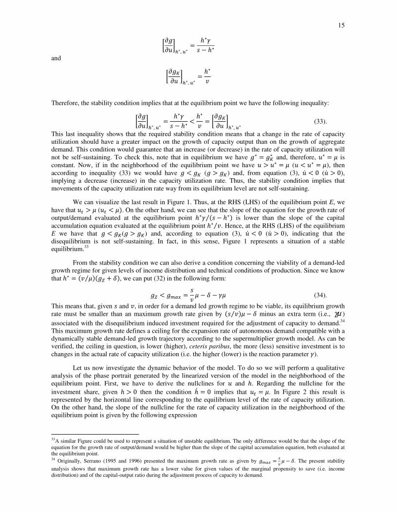
Therefore, the stability condition implies that at the equilibrium point we have the following inequality:

LF�F�M5∗,7∗ = ℎ∗,� − ℎ∗ < ℎ∗� = LF��F� M5∗,7∗ (33).

This last inequality shows that the required stability condition means that a change in the rate of capacity

utilization should have a greater impact on the growth of capacity output than on the growth of aggregate

demand. This condition would guarantee that an increase (or decrease) in the rate of capacity utilization will

not be self-sustaining. To check this, note that in equilibrium we have �∗ = ��∗ and, therefore, �∗ = - is

constant. Now, if in the neighborhood of the equilibrium point we have � > �∗ = - (� < �∗ = -), then

according to inequality (33) we would have � < �� (� > ��) and, from equation (3), �� < 0 (�� > 0),

implying a decrease (increase) in the capacity utilization rate. Thus, the stability condition implies that

movements of the capacity utilization rate way from its equilibrium level are not self-sustaining.

We can visualize the last result in Figure 1. Thus, at the RHS (LHS) of the equilibrium point E, we

have that �� > - (�� < -�. On the other hand, we can see that the slope of the equation for the growth rate of

output/demand evaluated at the equilibrium point ℎ∗, �� − ℎ∗�⁄ is lower than the slope of the capital

accumulation equation evaluated at the equilibrium point ℎ∗ �⁄ . Hence, at the RHS (LHS) of the equilibrium

E we have that � < ��(� > ��) and, according to equation (3), �� < 0 (�� > 0), indicating that the

disequilibrium is not self-sustaining. In fact, in this sense, Figure 1 represents a situation of a stable

equilibrium.33

From the stability condition we can also derive a condition concerning the viability of a demand-led

growth regime for given levels of income distribution and technical conditions of production. Since we know

that ℎ∗ = �� -⁄ ���( + ��, we can put (32) in the following form:

�( < �WXY = �� - − � − ,- (34).

This means that, given � and �, in order for a demand led growth regime to be viable, its equilibrium growth

rate must be smaller than an maximum growth rate given by �� �⁄ �- − � minus an extra term (i.e., γµ )

associated with the disequilibrium induced investment required for the adjustment of capacity to demand.34

This maximum growth rate defines a ceiling for the expansion rate of autonomous demand compatible with a

dynamically stable demand-led growth trajectory according to the supermultiplier growth model. As can be

verified, the ceiling in question, is lower (higher), ceteris paribus, the more (less) sensitive investment is to

changes in the actual rate of capacity utilization (i.e. the higher (lower) is the reaction parameter ,).

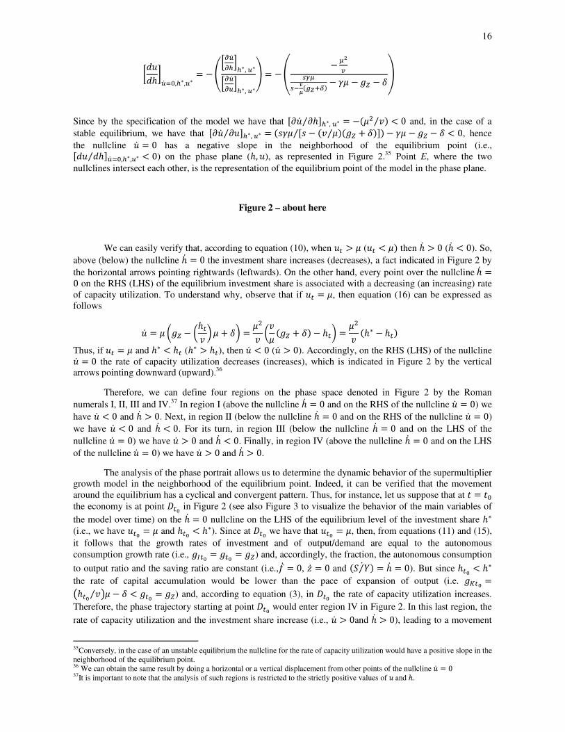
Let us now investigate the dynamic behavior of the model. To do so we will perform a qualitative

analysis of the phase portrait generated by the linearized version of the model in the neighborhood of the

equilibrium point. First, we have to derive the nullclines for � and ℎ. Regarding the nullcline for the

investment share, given ℎ > 0 then the condition ℎ� = 0 implies that �� = -. In Figure 2 this result is

represented by the horizontal line corresponding to the equilibrium level of the rate of capacity utilization.

On the other hand, the slope of the nullcline for the rate of capacity utilization in the neighborhood of the

equilibrium point is given by the following expression

33A similar Figure could be used to represent a situation of unstable equilibrium. The only difference would be that the slope of the

equation for the growth rate of output/demand would be higher than the slope of the capital accumulation equation, both evaluated at

the equilibrium point. 34 Originally, Serrano (1995 and 1996) presented the maximum growth rate as given by �WXY = Z@ - − �. The present stability

analysis shows that maximum growth rate has a lower value for given values of the marginal propensity to save (i.e. income

distribution) and of the capital-output ratio during the adjustment process of capacity to demand.

16

LE�EℎM7� [>,5∗,7∗ = −B\]7�]5^5∗,7∗\]7�]7^5∗,7∗C = −_ − A`@ZaAZbcd�efgh� − ,- − �( − �i

Since by the specification of the model we have that 8F�� Fℎ⁄ 95∗,7∗ = −�-Q �⁄ � < 0 and, in the case of a

stable equilibrium, we have that 8F�� F�⁄ 95∗,7∗ = ��,- 8� − �� -⁄ ���( + ��9⁄ � − ,- − �( − � < 0, hence

the nullcline �� = 0 has a negative slope in the neighborhood of the equilibrium point (i.e., 8E� Eℎ⁄ 97� [>,5∗,7∗ < 0) on the phase plane (ℎ, �), as represented in Figure 2.35 Point E, where the two

nullclines intersect each other, is the representation of the equilibrium point of the model in the phase plane.

Figure 2 – about here

We can easily verify that, according to equation (10), when �� > - (�� < -� then ℎ� > 0 (ℎ� < 0). So,

above (below) the nullcline ℎ� = 0 the investment share increases (decreases), a fact indicated in Figure 2 by

the horizontal arrows pointing rightwards (leftwards). On the other hand, every point over the nullclineℎ� =0 on the RHS (LHS) of the equilibrium investment share is associated with a decreasing (an increasing) rate

of capacity utilization. To understand why, observe that if �� = -, then equation (16) can be expressed as

follows

�� = - ��( − �ℎ�� �- + �� = -Q� ��- ��( + �� − ℎ�� = -Q� �ℎ∗ − ℎ��

Thus, if �� = - and ℎ∗ < ℎ� (ℎ∗ > ℎ�), then �� < 0 (�� > 0). Accordingly, on the RHS (LHS) of the nullcline �� = 0 the rate of capacity utilization decreases (increases), which is indicated in Figure 2 by the vertical

arrows pointing downward (upward).36

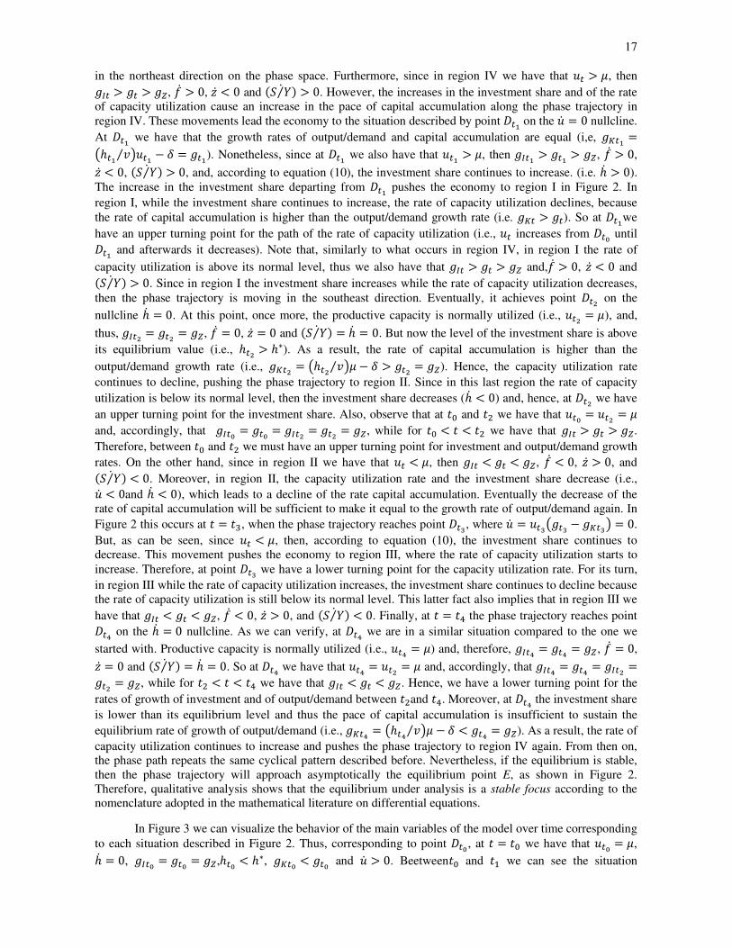
Therefore, we can define four regions on the phase space denoted in Figure 2 by the Roman

numerals I, II, III and IV.37

In region I (above the nullcline ℎ� = 0 and on the RHS of the nullcline �� = 0) we

have �� < 0 and ℎ� > 0. Next, in region II (below the nullcline ℎ� = 0 and on the RHS of the nullcline �� = 0)

we have �� < 0 and ℎ� < 0. For its turn, in region III (below the nullcline ℎ� = 0 and on the LHS of the

nullcline �� = 0) we have �� > 0 and ℎ� < 0. Finally, in region IV (above the nullcline ℎ� = 0 and on the LHS

of the nullcline �� = 0) we have �� > 0 and ℎ� > 0.

The analysis of the phase portrait allows us to determine the dynamic behavior of the supermultiplier

growth model in the neighborhood of the equilibrium point. Indeed, it can be verified that the movement

around the equilibrium has a cyclical and convergent pattern. Thus, for instance, let us suppose that at ? = ?>

the economy is at point ��j in Figure 2 (see also Figure 3 to visualize the behavior of the main variables of

the model over time) on the ℎ� = 0 nullcline on the LHS of the equilibrium level of the investment share ℎ∗ (i.e., we have ��j = - and ℎ�j < ℎ∗). Since at ��j we have that ��j = -, then, from equations (11) and (15),

it follows that the growth rates of investment and of output/demand are equal to the autonomous

consumption growth rate (i.e., �+�j = ��j = �() and, accordingly, the fraction, the autonomous consumption

to output ratio and the saving ratio are constant (i.e.,!� = 0, � = 0 and �� �⁄ �� = ℎ� = 0). But since ℎ�j < ℎ∗ the rate of capital accumulation would be lower than the pace of expansion of output (i.e. ���j ="ℎ�j �⁄ #- − � < ��j = �() and, according to equation (3), in ��j the rate of capacity utilization increases.

Therefore, the phase trajectory starting at point ��j would enter region IV in Figure 2. In this last region, the

rate of capacity utilization and the investment share increase (i.e., �� > 0and ℎ� > 0), leading to a movement

35Conversely, in the case of an unstable equilibrium the nullcline for the rate of capacity utilization would have a positive slope in the

neighborhood of the equilibrium point. 36 We can obtain the same result by doing a horizontal or a vertical displacement from other points of the nullcline �� = 0 37It is important to note that the analysis of such regions is restricted to the strictly positive values of �and ℎ.

17

in the northeast direction on the phase space. Furthermore, since in region IV we have that �� > -, then �+� > �� > �(, !� > 0, � < 0 and �� �⁄ �� > 0. However, the increases in the investment share and of the rate

of capacity utilization cause an increase in the pace of capital accumulation along the phase trajectory in

region IV. These movements lead the economy to the situation described by point ��k on the �� = 0 nullcline.

At ��k we have that the growth rates of output/demand and capital accumulation are equal (i,e, ���k ="ℎ�k �⁄ #��k − � = ��k). Nonetheless, since at ��k we also have that ��k > -, then �+�k > ��k > �(, !� > 0, � < 0, �� �⁄ �� > 0, and, according to equation (10), the investment share continues to increase. (i.e. ℎ� > 0).

The increase in the investment share departing from ��k pushes the economy to region I in Figure 2. In

region I, while the investment share continues to increase, the rate of capacity utilization declines, because

the rate of capital accumulation is higher than the output/demand growth rate (i.e. ��� > ��). So at ��kwe

have an upper turning point for the path of the rate of capacity utilization (i.e., �� increases from ��j until ��k and afterwards it decreases). Note that, similarly to what occurs in region IV, in region I the rate of

capacity utilization is above its normal level, thus we also have that �+� > �� > �( and,!� > 0, � < 0 and �� �⁄ �� > 0. Since in region I the investment share increases while the rate of capacity utilization decreases,

then the phase trajectory is moving in the southeast direction. Eventually, it achieves point ��` on the

nullcline ℎ� = 0. At this point, once more, the productive capacity is normally utilized (i.e., ��` = -), and,

thus, �+�` = ��` = �(, !� = 0, � = 0 and �� �⁄ �� = ℎ� = 0. But now the level of the investment share is above

its equilibrium value (i.e., ℎ�` > ℎ∗). As a result, the rate of capital accumulation is higher than the

output/demand growth rate (i.e., ���` = "ℎ�` �⁄ #- − � > ��` = �(). Hence, the capacity utilization rate

continues to decline, pushing the phase trajectory to region II. Since in this last region the rate of capacity

utilization is below its normal level, then the investment share decreases (ℎ� < 0) and, hence, at ��` we have

an upper turning point for the investment share. Also, observe that at ?> and ?Q we have that ��j = ��` = -

and, accordingly, that �+�j = ��j = �+�` = ��` = �(, while for ?> < ? < ?Q we have that �+� > �� > �(.

Therefore, between ?> and ?Q we must have an upper turning point for investment and output/demand growth

rates. On the other hand, since in region II we have that �� < -, then �+� < �� < �(, !� < 0, � > 0, and �� �⁄ �� < 0. Moreover, in region II, the capacity utilization rate and the investment share decrease (i.e., �� < 0and ℎ� < 0), which leads to a decline of the rate capital accumulation. Eventually the decrease of the

rate of capital accumulation will be sufficient to make it equal to the growth rate of output/demand again. In

Figure 2 this occurs at ? = ?l, when the phase trajectory reaches point ��m, where �� = ��m"��m − ���m# = 0.

But, as can be seen, since �� < -, then, according to equation (10), the investment share continues to

decrease. This movement pushes the economy to region III, where the rate of capacity utilization starts to

increase. Therefore, at point ��m we have a lower turning point for the capacity utilization rate. For its turn,

in region III while the rate of capacity utilization increases, the investment share continues to decline because

the rate of capacity utilization is still below its normal level. This latter fact also implies that in region III we

have that �+� < �� < �(, !� < 0, � > 0, and �� �⁄ �� < 0. Finally, at ? = ?n the phase trajectory reaches point ��o on the ℎ� = 0 nullcline. As we can verify, at ��o we are in a similar situation compared to the one we

started with. Productive capacity is normally utilized (i.e., ��o = -) and, therefore, �+�o = ��o = �(, !� = 0, � = 0 and �� �⁄ �� = ℎ� = 0. So at ��o we have that ��o = ��` = - and, accordingly, that �+�o = ��o = �+�` =��` = �(, while for ?Q < ? < ?n we have that �+� < �� < �(. Hence, we have a lower turning point for the

rates of growth of investment and of output/demand between ?Qand ?n. Moreover, at ��o the investment share

is lower than its equilibrium level and thus the pace of capital accumulation is insufficient to sustain the

equilibrium rate of growth of output/demand (i.e., ���o = "ℎ�o �⁄ #- − � < ��o = �(). As a result, the rate of

capacity utilization continues to increase and pushes the phase trajectory to region IV again. From then on,

the phase path repeats the same cyclical pattern described before. Nevertheless, if the equilibrium is stable,

then the phase trajectory will approach asymptotically the equilibrium point E, as shown in Figure 2.

Therefore, qualitative analysis shows that the equilibrium under analysis is a stable focus according to the

nomenclature adopted in the mathematical literature on differential equations.

In Figure 3 we can visualize the behavior of the main variables of the model over time corresponding

to each situation described in Figure 2. Thus, corresponding to point ��j, at ? = ?> we have that ��j = -, ℎ� = 0, �+�j = ��j = �(,ℎ�j < ℎ∗, ���j < ��j and �� > 0. Beetween?> and ?p we can see the situation

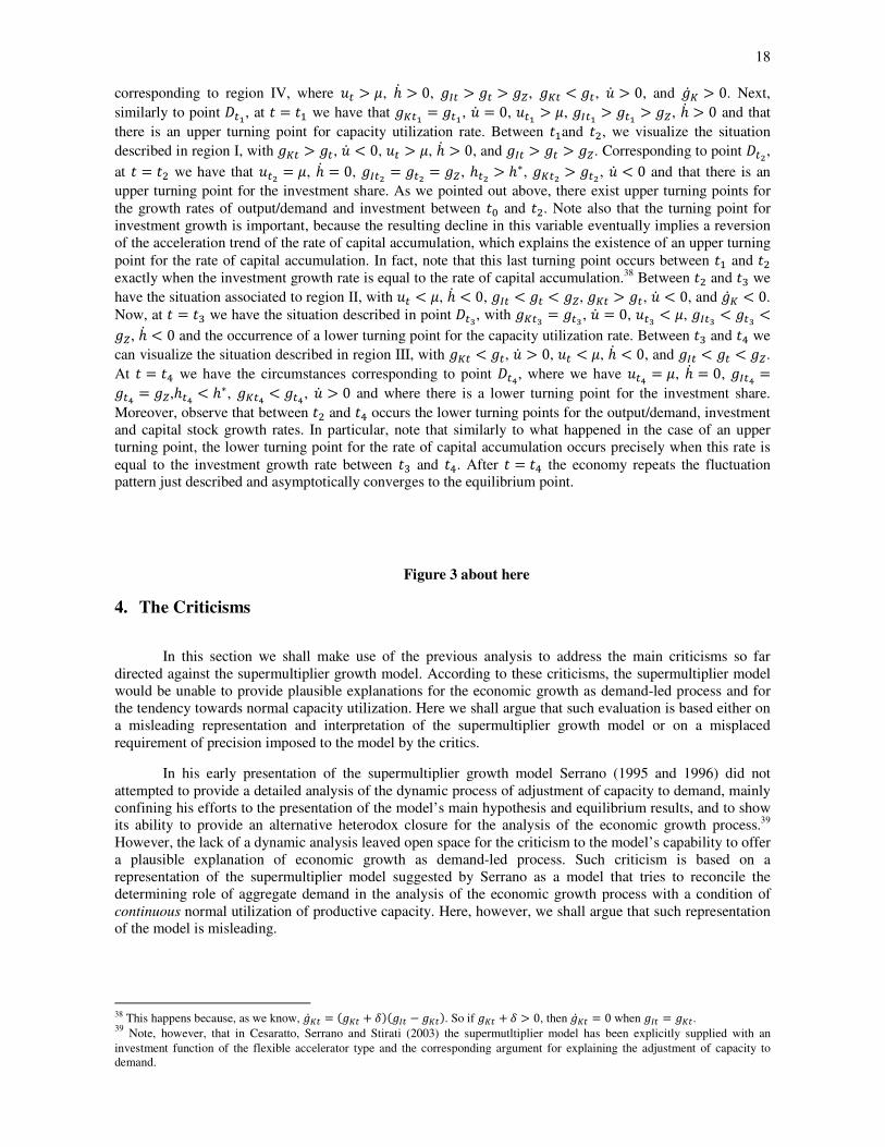
18

corresponding to region IV, where �� > -, ℎ� > 0, �+� > �� > �(, ��� < ��, �� > 0, and ��� > 0. Next,

similarly to point ��k, at ? = ?p we have that ���k = ��k, �� = 0, ��k > -, �+�k > ��k > �(, ℎ� > 0 and that

there is an upper turning point for capacity utilization rate. Between ?pand ?Q, we visualize the situation

described in region I, with ��� > ��, �� < 0, �� > -, ℎ� > 0, and �+� > �� > �(. Corresponding to point ��`,

at ? = ?Q we have that ��` = -, ℎ� = 0, �+�` = ��` = �(, ℎ�` > ℎ∗, ���` > ��`, �� < 0 and that there is an

upper turning point for the investment share. As we pointed out above, there exist upper turning points for

the growth rates of output/demand and investment between ?> and ?Q. Note also that the turning point for

investment growth is important, because the resulting decline in this variable eventually implies a reversion

of the acceleration trend of the rate of capital accumulation, which explains the existence of an upper turning

point for the rate of capital accumulation. In fact, note that this last turning point occurs between ?p and ?Q

exactly when the investment growth rate is equal to the rate of capital accumulation.38 Between ?Q and ?l we

have the situation associated to region II, with �� < -, ℎ� < 0, �+� < �� < �(, ��� > ��, �� < 0, and ��� < 0.

Now, at ? = ?l we have the situation described in point ��m, with ���m = ��m, �� = 0, ��m < -, �+�m < ��m <�(, ℎ� < 0 and the occurrence of a lower turning point for the capacity utilization rate. Between ?l and ?n we

can visualize the situation described in region III, with ��� < ��, �� > 0, �� < -, ℎ� < 0, and �+� < �� < �(.

At ? = ?n we have the circumstances corresponding to point ��o, where we have ��o = -, ℎ� = 0, �+�o =��o = �(,ℎ�o < ℎ∗, ���o < ��o , �� > 0 and where there is a lower turning point for the investment share.

Moreover, observe that between ?Q and ?n occurs the lower turning points for the output/demand, investment

and capital stock growth rates. In particular, note that similarly to what happened in the case of an upper

turning point, the lower turning point for the rate of capital accumulation occurs precisely when this rate is

equal to the investment growth rate between ?l and ?n. After ? = ?n the economy repeats the fluctuation

pattern just described and asymptotically converges to the equilibrium point.

Figure 3 about here

4. The Criticisms

In this section we shall make use of the previous analysis to address the main criticisms so far

directed against the supermultiplier growth model. According to these criticisms, the supermultiplier model

would be unable to provide plausible explanations for the economic growth as demand-led process and for

the tendency towards normal capacity utilization. Here we shall argue that such evaluation is based either on

a misleading representation and interpretation of the supermultiplier growth model or on a misplaced

requirement of precision imposed to the model by the critics.

In his early presentation of the supermultiplier growth model Serrano (1995 and 1996) did not

attempted to provide a detailed analysis of the dynamic process of adjustment of capacity to demand, mainly

confining his efforts to the presentation of the model’s main hypothesis and equilibrium results, and to show

its ability to provide an alternative heterodox closure for the analysis of the economic growth process.39

However, the lack of a dynamic analysis leaved open space for the criticism to the model’s capability to offer

a plausible explanation of economic growth as demand-led process. Such criticism is based on a

representation of the supermultiplier model suggested by Serrano as a model that tries to reconcile the

determining role of aggregate demand in the analysis of the economic growth process with a condition of

continuous normal utilization of productive capacity. Here, however, we shall argue that such representation

of the model is misleading.

38 This happens because, as we know, ���� = ���� + ����+� − ����. So if ��� + � > 0, then ���� = 0 when �+� = ���. 39

Note, however, that in Cesaratto, Serrano and Stirati (2003) the supermutltiplier model has been explicitly supplied with an

investment function of the flexible accelerator type and the corresponding argument for explaining the adjustment of capacity to

demand.

19

In order to show that, let us suppose that at ? = 0 the economy is characterized by the normal

utilization of productive capacity and that the level of capacity output determines the normal output level, so

that we have

�> = -� > .40

Further, given the level of income distribution and given the value of autonomous consumption at ? = 0, the

initial level of consumption is also determined at ? = 0, such as �> = �> +��>. Thus, in order to have an

equilibrium between aggregate demand and aggregate output, aggregate investment at ? = 0 must assume the

following required value �> = ��> − �> = �> − �> = �>

So, at ? = 0, Say’s law prevails, aggregate demand is determined by the level of normal output and normal

capacity savings determines investment. Now let us suppose we are interested to know the rate of expansion

of aggregate demand that would be required to continuously maintain the equilibrium between aggregate

demand and output and the normal utilization of productive capacity through time (i.e., the fully adjusted

equilibrium). In order to maintain the normal utilization of productive capacity, aggregate output must grow

at the same rate as capacity output, and then aggregate demand would also have to grow at this same rate.

Under the present circumstances, the rate of growth of capacity output would be given by

�� = ��� = ��� ��⁄ �� - = �� − �� ��⁄ �� -

Thus aggregate output and demand would be required to grow at the above rate in order to continuously

maintain the economy in a fully adjusted equilibrium. As can be easily verified such growth rate is

equivalent to the warranted rate of growth suggested by Harrod (1939 and 1948) when we take into account

the existence of an autonomous component in aggregate consumption.

Nonetheless, the existence of this autonomous component growing at an independent growth rate

implies that the warranted rate growth would, in general, change through time. Actually, the dynamic

behavior of the warranted growth rate incorporating the autonomous consumption component can be

expressed by the following differential equation

�� = -� ��� − �(� ���� = ��� − �(� q�� - − ��r

As can be seen from the equation above, the model has two stationary points, ��∗ = �( and ��∗∗ = �� �⁄ �-.

Now, let us assume that the values of �, �, - and �( are such that �� �⁄ �- > �(. Thus, we have three

possible outcomes depending on the initial situation regarding the relationship between the warranted and

autonomous consumption growth rates. That is at ? = 0 we may have three possible relations between these

two rates

�> = �� − �> �>⁄ �� - ⋛ �(

For the sake of future discussion, it is important to observe that these initial conditions can be alternatively

represented by the corresponding relations bellow

�> ⋛ �>� − @A �(

Note that the latter relations are in fact deduced from the former relations (i.e. �> ⋛ �( ⇒ �> ⋛�> �� − �� -⁄ ��(�⁄ . Thus, they should only be interpreted as an alternative way to present the relations

between the warranted and autonomous consumption growth rates. In particular, it is not legitimate to

interpret the situation �> = �> �� − �� -⁄ ��(�⁄ as representing the equilibrium level of output determined by

the supermultiplier growth model. Although it seems to be so (see equation (23) above), in fact, as we

already asserted, the expression is only an alternative way to present the situation according to which the

warranted and the autonomous consumption growth rates happens to be equal to each other at ? = 0. The

40

For the sake of the discussion in this section, let us suppose here that � = 0, which implies that net and gross figures for output,

income, profits, investment and savings are equal to each other.

20

level of (normal) output at ? = 0 is determined by the level of capacity output and, therefore, does not

depend on the level of aggregate demand and it is not determined by the RHS of the equation above. In fact,

as our argument above shows, aggregate output and demand are equal to each other throughout time,

including ? = 0, in the three situations previously defined.

Now we can analyze the behavior of the warranted rate through time depending on the initial

relations between that rate and the rate of growth of autonomous consumption previously described. Thus if

we have initially �> > �( then, according to the equation above, �� = �- �⁄ ���> − �(���> �>⁄ � > 0 at ? = 0.

It follows that �� > �( for all ? > 0 and, therefore, we obtain �� ��⁄ → 0 and � → �� �⁄ �- as ? → ∞. That is,

in this case, the warranted rate asymptotically converges to �� �⁄ �-, the value of the warranted rate without

autonomous consumption.41 On the other hand, if initially �> < �( then �� = �- �⁄ ���> − �(���> �>⁄ � < 0.

As a result we have �� < �( and �� < 0 for an interval of time immediately after ? = 0. In this case,

eventually we must have �� < 0 and, therefore, after some time with the economy growing at a negative rate,

we would achieve a zero level of aggregate output. So in these circumstances, the economy collapses until it

achieves a floor where the level of output is equal to zero. Finally, if we have initially �> = �( then, from

the equation representing the dynamics of the warranted growth rate, we would obtain that the warranted

growth rate would be constant through time (i.e. we would have �� = �> = �( for all ?). So, if the warranted

growth rate happens to be equal to the growth rate of autonomous consumption at ? = 0 then such equality

would be maintained through time. It is important to be remarked, however, that the latter situation should

not be interpreted as an equilibrium state where the rate of growth of autonomous consumption determines

the rate of growth of output. Actually, the latter situation is only the result of a coincidence. Accordingly, the

divergence of the warranted growth rate from the rate of growth of autonomous consumption obtained in the

other two situations previously analyzed cannot also be interpreted as an evidence of the instability of a

supposed equilibrium growth path according to which output would grow at a rate determined by the pace of

expansion of autonomous consumption. 42

More generally, the assumption that the growth rates of aggregate

demand and actual output are always the ones required to continuously maintain the normal utilization of

productive capacity implies that the specific model here investigated is in fact a formalization of the

economic growth process based on the validity of Say’s law. Thus the model under analysis specifically

shows the characteristics of the growth path based on Say’s law when one component of aggregate demand

grows at rate independent from the rate of growth of aggregate output and demand.

Hence, although Serrano’s (1995 and 1996) declared intention was to provide an alternative

heterodox growth model based on “the validity of the Keynesian-Kaleckian principle of effective demand in

the long run”,43 his supermultiplier growth model has been represented by the model described above, that is,

as we saw, a growth model based on Say’s law. This is the source of the misleading interpretation of

Serrano’s supermultiplier model found in Trezzini (1998), Schefold (2000) and Barbosa-Filho (2000).44

To show that this is the case, from the equation of the warranted rate it follows that

�� = ��-����� = ��� − �� .

The equation above determines the level of investment required to maintain the normal utilization of

productive capacity through time. Now if, besides assuming normal utilization of productive capacity at ? = 0, we also suppose that capitalist firms perfectly foresee the behavior of the warranted rate of growth

41

Observe that while the warranted rate asymptotically converges to �� �⁄ �-, the growth trajectory presents an implausible pattern

according to which the investment share of output increases throughout the whole path converging to the value of the marginal

propensity to save (i.e. �� �� → �⁄ ) 42 Note that notwithstanding the fact that the model is based on the notion of a warranted growth rate, it does not deal with the

problem of instability of the warranted growth rate pointed out by Harrod. Actually, in the model it is supposed that the actual growth

rate of output is always equal to the warranted rate throughout the growth paths generated by the model. 43 According to Serrano (1995 and 1996) the trend level and rate of growth of autonomous demand is supposed to determine the

trend level and rate of growth of capacity output. 44 Park (2000) also represents the supermultiplier model along these lines, but the focus of his paper is on the dependence of the

warranted rate of growth on the rate of growth of autonomous demand. From the existence of this dependence the author concludes

that effective demand is an important element in the process of economic growth. Our analysis, however, shows that the model under

analysis (but not the supermultiplier model) is based on Say’s Law. Thus, such model is not compatible with the notion of effective

demand as a main determinant of the level of aggregate output.

21

according to the model presented above,45

it follows that the expression �� = �� -⁄ ����� can be interpreted as

an unlagged version of the accelerator investment function. In this case, the investment level determined by

the accelerator investment function would be able to maintain the normal utilization of productive capacity

throughout the entire growth path. But note that, under the stringent conditions suggested, the investment

level determined by the unlagged accelerator investment function is nothing more than the level of required

investment determined by normal capacity savings. Thus the level of investment is not independent from the

level of normal capacity savings, and we are still under the rule of Say’s Law.

Trezzini (1998), Schefold (2000) and Barbosa-Filho (2000) used this specific version of the

accelerator investment function, combined with the assumptions of continuous equilibrium between

aggregate demand and output and of initial normal utilization of productive capacity, in their representation

and interpretation of Serrano’s Supermultiplier.46 In fact, substituting such investment function into the

equilibrium condition between aggregate demand and output, we obtain the following first order ordinary

differential equation

��-��� − ��� + �>uef� = 0

Apart from differences in notation, this is essentially the same differential equation used by Schefold (2000,

p. 345) and Barbosa-Filho (2000, p. 31) to analyze the dynamic behavior of the supermultiplier model.

Following Schefold (2000, p. 345),47,48 the general solution of the above equation is given by

�� = B �>� − q@Ar�(Cuef� + B�> − �>� − q@Ar�(CuqvcAr�

Recalling that we are supposing that �� �⁄ �- > �(, the above equation provides us with the same solutions

obtained previously depending on the three possible initial conditions. Thus if �> > �> �� − �� -⁄ ��(�⁄ (i.e.,

as we saw, when �> > �() then the economy would converge asymptotically to an equilibrium path where � = �� �⁄ �-. On the other hand, if �> < �> �� − �� -⁄ ��(�⁄ (i.e., as we saw, when �> < �() then the

economy would collapse until it reaches the floor associated with a zero level of economic activity. Finally,

when we have initially a situation according to which �> = �> �� − �� -⁄ ��(�⁄ (i.e., as we saw, when �> = �() the economy would be, by a fluke, in an equilibrium path where � = �( for all ? ≥ 0. Thus the

model used by Trezzini, Schefold and Barbosa-Filho describes the dynamics of the rate of growth of output

45

It should be remarked that what we have here is an assumption that is stronger than the assumption of perfect foresight on the part

of capitalist firms. In fact, we are supposing that, in their investment decisions, capitalist firms are able to behave consistently with

the model’s assumption according to which aggregate demand exactly grows at a rate required to maintain normal capacity utilization

throughout the whole growth path. In this sense, capitalist firms would have to be interested in predicting the behavior of warranted

rate of growth, and not the behavior of aggregate demand growth rate as such. There is no reason to believe that this would be the

kind of behavior induced by capitalist competition. 46 Trezzini (1995 and 1998) claims that the model under discussion also represents Hicks’ supermultiplier model (Hicks, 1950).

However, Hicks uses a lagged version of the accelerator investment function to study the cyclical behavior associated with the

multiplier/accelerator interaction under the constraints of a full employment ceiling and zero gross investment floor. In this sense, it

is important to note that Hicks’ supermultiplier model generates fluctuations of the rate of capacity utilization and not a fully adjusted

growth path. Thus, the model with continuous normal utilization of productive capacity under analysis does not adequately represent

Hicks’ supermultiplier as well. Nevertheless, it confirms and extends to the case of an economy with an autonomous demand

component Garegnani’s (Garegnani, 1992) argument according to which the combination of continuous normal utilization with a

given level of income distribution is incompatible with the application of the principle of effective demand to the analysis of the

economic growth process. 47 Schefold (2000, p. 345) refers to the solution for the above differential equation that can be found in Allen (1968, p. 343). In this

connection, it is interesting to note that Allen calls the model under discussion “Equilibrium accelerator-multiplier model”. This

designation tries to capture the fact that with the use of an unlagged accelerator investment function the model can only discuss the

dynamics of the equilibrium growth rate (the modified warranted growth rate). Thus, such model would be unable to deal with the

(harrodian) disequilibrium problems associated with the divergence of the actual output/demand growth rate from the equilibrium

growth rate. In fact, Allen (1968, p. 346) makes use of a disequilibrium accelerator-multiplier model, with a lagged accelerator

investment function, in order to deal with the possible disequilibrium process between actual and equilibrium growth rates in the

presence of a growing autonomous expenditure. In this sense, we think that is not legitimate to refer to the harrodian knife edge

instability process in the context of the model under discussion as Schefold (2000, p. 345) does. 48

Barbosa-Filho (2000, p. 31), discusses the dynamic behavior of the model under analysis based on the nonlinear first order

differential equation of the Riccati type deduced from the differential equation for the level of output presented above. The equation

he uses is essentially the same as the one we used above to discuss the behavior of the model. That is, in our notation, he analyzes the

behavior of the model according to the equation �� = ��� − �(�"�� �⁄ �- − ��# = −��Q + ��( + �� �⁄ �-��� − �� �⁄ �-�(.

22

that allows the continuous maintenance of the equilibrium between aggregate output and demand and the

continuous normal utilization of productive capacity (i.e. the harrodian warranted growth rate). That is, the

model under analysis would always generate a continuous fully adjusted growth path. Therefore, it is not

surprising that if such model could be considered a reasonable representation of the supermultiplier growth

model, then the only possible conclusion would be that the latter model would be unable to provide a

plausible demand-led explanation for the process of economic growth. However our analysis in the present

paper shows that such conclusion is based on a misleading representation of the supermultiplier growth

model. The model used to represent the supermultiplier growth model is, in reality, a model based on the

Say’s Law, a model according to which the level of investment is determined by level of normal capacity

savings.

Contrary to the analysis based on the misleading representation of the supermultiplier growth model

provided by the model discussed above, in our presentation of the supermultiplier model we showed that the

level of aggregate demand determines the level of aggregate output. Further, our previous analysis of the

dynamic behavior of the model clearly has shown that it generates trajectories that are not continuously fully

adjusted. As can be verified in Figures 2 and 3 and the corresponding discussion above, the model produces

growth paths characterized by deviations of the actual rate of capacity utilization from its normal level. In

fact, according to the model, it is exactly the influence of such deviations on the investment share of output

(i.e. the marginal propensity to invest) that makes it possible for the model to explain the eventual

convergence of the actual growth path of output to the trend expansion path of autonomous demand and also

the tendency towards normal utilization of productive capacity. In this sense, the divergences between actual

and normal rates of capacity utilization are an essential element in the theoretical account of the adjustment

process of capacity to aggregate demand provided by the supermultiplier growth model. Hence, according to

the latter, the reaction of the rate of capital accumulation to changes in the trend rate of autonomous demand

growth in a capitalist economy relies on both, changes in the rate of capacity utilization and changes in the

investment share of output. Actually, it should be noted, the model shows that these changes are

complementary to each other. For, in the case of an unexpected increase in the trend rate of autonomous

demand growth, the first reaction of the economy is an increase in the rate of capacity utilization and,

accordingly, a relatively fast increase in the rate of capital accumulation, which are only possible because the

system operates with margins of planned spare capacity. On the other hand, it is the tendency for an increase

in the investment share of output that ultimately explains the long run adjustment of the rate of capital

accumulation to the trend rate of autonomous demand growth; while, at the same time, such tendency

restores the margins of planned spare capacity and, hence, the ability of the economy to react to further

changes in the trend rate of autonomous demand growth. Therefore, the combined changes in the rate of

capacity utilization and in the investment share of output subjacent to the process of adjustment of capacity

to aggregate demand associated with the supermultiplier growth model offer a plausible demand-led

explanation for the long run process of economic growth. In this sense, the supermultiplier growth model

proves to be able to extend the applicability of the Keynesian-Kaleckian principle of effective demand to the

context of analysis of long run economic growth and that this extension is fully compatible with the tendency

towards the normal utilization of productive capacity.

Observe also that the assumption of continuous normal utilization adopted by Trezzini, Schefold and

Barbosa-Filho in their representation of the supermultiplier growth model implies that the actual growth rates

of output and capital stock are always equal to the warranted rate of growth. In contrast, according to our

analysis of the supermultiplier growth model, these rates are only equal to each other in the equilibrium path

of the model, where they are all determined by rate of growth of autonomous consumption (see equation (18)

above). Outside the equilibrium path, these rates are, in general, different to each other. The warranted rate

of growth is equal to the notional rate of capital accumulation that would be obtained if capacity utilization

were normally utilized. That is, from equation (2) and recalling that we are supposing in this section that �=0, we would have in this case

��� = �ℎ�� �- = q� − �� r-

It follows that the supermultiplier growth model determines the warranted growth rate endogenously. The

latter depends, ceteris paribus, on the value of the investment share of output and, thus, it varies according to

changes in the investment share of output along the process of adjustment of capacity to demand. Moreover,

23

as a comparison with equation (2) demonstrates, the warranted rate is related to the actual rate of capital

accumulation as follows ��� ⋛ ���as�� ⋛ -

We can verify that the actual rate of capital accumulation exhibits more variability than the warranted rate of

growth since, although both rates positively depend on the investment share of output, the former also

depends positively on the actual rate of capacity utilization. This confirms the importance of the variability

of the actual rate of capacity utilization in the process of adjustment of capacity to demand. The variability of

the actual rate of capacity utilization allowed by the existence of margins of spare capacity increases the

responsiveness of the pace of capital accumulation and, thus, of the expansion of productive capacity to the

stimulus provided by the demand-led growth process. Further, the two rates are only equal to each other

when the rate of capacity utilization happens to be equal to its normal level, a situation that is not sustainable

outside the equilibrium path. But when the latter path is stable, the values of the three rates of growth tend to

converge to the rate of growth of autonomous consumption. Figure 4 illustrates the relationship between the

warranted rate of growth, the rate of growth of output/demand and the actual pace of capital accumulation

discussed above. Finally, it should be remarked that, in the context of the supermultiplier growth model, the

warranted rate of growth loses much of its significance. For, on the one hand, outside the equilibrium path

nothing grows at the warranted rate and the latter does not exert any influence on the dynamic behavior of

model. On the other hand, in the equilibrium path of the model, the rate of growth of autonomous

consumption determines the warranted rate of growth and, therefore, the latter does not have a determining

role in the equilibrium path also.

Figure 4 about here

The ability of the supermultiplier growth model to provide a plausible explanation for the economic

growth process from a demand-led point of view has also been questioned by Palumbo & Trezzini (2003) on

the ground that the model supposedly requires the equality between the time average value of the actual rate

of capacity utilization and its normal level. Here, however, we shall argue that this requirement is simply too

strong and is not necessary for the validity of the model’s conclusions. As argued by Vianello (1989) in

relation to the analysis of the gravitation process of market to normal prices, requiring the equality between

the time average of market prices and normal prices implies the validity of the implausible hypothesis of

reciprocal compensation of the divergences between them. Since, as convincingly argued by Ciccone (1990),

the gravitation of market to normal prices would be faster than the adjustment of capacity to demand, then it

seems to be reasonable to believe that the requirement under discussion is even more stringent when applied

to the investigation of the latter adjustment process. Such would be the case because the relation between

average and normal rates of capacity utilization is almost always sensitive to the initial conditions present in

the dynamic analysis, to the arbitrary time period used to calculate the time average of actual values and to

the prevalence of any non-random pattern of change in exogenous variables. Actually, the restrictive and

arbitrary nature of the requirement under discussion is evident from the fact that it fails to distinguish

between an unstable and a stable adjustment process of capacity to demand, both of which would not be able

to meet such requirement in normal conditions. Thus, in general, we are only able to assert the existence of a

tendency for the actual rate of capacity utilization to converge to its normal (or equilibrium) level49 which is

exactly what the stability analysis pursued above allows us to assert. Requiring more than that would impose

a level of precision to the analysis that is not achievable in general, being a kind of misplaced exigency of

precision.

Finally, Palumbo & Trezzini (2003) also questions whether the supermultiplier model would be able

to plausibly guarantee the existence of a tendency for the actual rate of capacity utilization to converge to its

normal (or equilibrium) level. First, they argue that such tendency would require the very strong assumptions

of perfect foresight and perfect knowledge on the part of capitalist firms in their investment decisions. In

contrast, our analysis of the supermultiplier model shows that these hyper-rational behavioral assumptions

are not needed. Actually, our analysis of the investment process is not intended to deal with the behavior of

individual capitalist firms in their particular or individual process of capital accumulation. The investment

function adopted in this paper is meant to capture the influence of capitalist competition process on the

49

Of course, when more specific knowledge is available from empirical inquiries, we may also be able to infer something about the

time profile and intensity characterizing such tendency.

24

behavior of aggregate investment.50

. So we suppose that if the actual rate of capacity utilization is above the

normal level (i.e. if the margins of spare capacity are on average below their planned levels), aggregate

capitalist investment would expand at a faster rate than aggregate demand (and output) because capitalist

firms would try restore the levels of planned spare capacity in order to avoid the possibility of losing market

share for not being able to meet peak levels of demand. On the other hand, if the actual rate of capacity

utilization is below the normal level (i.e. if the margins of spare capacity are on average above their planned

levels), we assume that capitalist investment would expand at a lower rate than aggregate demand (and

output) since, in this situation, capitalist firms would be able to increase their profitability without

compromising their market shares. As can be verified, our reasoning does not involve any of the hyper-

rational assumptions suggested by Palumbo and Trezzini, and yet we are able to show that, under the

conditions stated in the last section, the model produces a tendency towards normal utilization of productive

capacity.51 Secondly, Palumbo and Trezzini argue that the tendency towards normal utilization of productive

capacity can be countervailed by other forces associated with the very process of capitalist competition that

would trigger such tendency. In particular, according to them, the adjustment of capacity to demand affects

aggregate demand through its effect over aggregate investment, which, according to the authors, would be

able to frustrate the latter adjustment process. Note, however that this is exactly the type of interaction

associated with the multiplier/accelerator mechanism that is built in the supermultiplier growth model. Thus,

we are already taking care of such countervailing force when we discuss the dynamic behavior and the

stability of the equilibrium path of the model. Indeed, we have seen that, although the process of adjustment

of capacity to demand unleashed by capitalist competition leads the economy in the right direction, the

intensity of the process may prevent the actual rate of capacity utilization to converge to its normal level.

Nonetheless, we also pointed out above that the latter convergence is assured if the stability condition is met,

which would be the case if we have a sufficiently low value of the parameter ,. Therefore, in this case, the

tendency towards normal utilization of productive capacity is not prevented by the multiplier/accelerator

interaction and we can overcome this last objection by Palumbo and Trezzini.52

5. A Comparison with alternative models53

In this section we shall compare the main results obtained in our discussion of the supermultiplier

growth model with alternative heterodox growth models that also deal with the relationship between

economic growth, income distribution and effective demand. More specifically, we will compare the

supermultiplier, Cambridge and neo-Kaleckian growth models trying to point out their similarities and, more

importantly, their main differences. The comparison will be made within the same simplified analytical

context used in the discussion of the supermultiplier model. Thus, the following assumptions will be

maintained: we have a closed capitalist economy without government; aggregate income is distributed in the

form of wages and profits; the method of production in use requires a fixed combination of homogeneous

labor input with homogeneous fixed capital to produce a single output; there is constant returns to scale and

no technological progress; and there exists a permanent labor surplus. Moreover, as occurred in the case of

50 With this procedure we try to avoid the problematic use of the representative agent type of reasoning on aggregate investment

theory. The problem with this approach follows from the fact that, although aggregate capitalist investment is the result of a

decentralized decision process by individual capitalist firms, their individual investment decisions are intrinsically connected by the

functioning of the process of inter-capitalist competition and the existence of these interconnections exerts an important influence on

individual capitalist decisions. 51

This part of the argument seems to rely on the misleading representation of the supermultiplier model proposed by Trezzini (1998)

that was discussed above. 52 Besides the latter objection, Palumbo and Trezzini (2003) also argue that capitalist competition induces the process of technical

change and the latter could hamper the tendency towards normal capacity utilization. In the present paper, we are not dealing with the

connections between the process of technical change and of adjustment of capacity to demand. In fact, in order to simplify our

analysis, we assumed away the existence of technical change from the start. Nevertheless, it is our position that the technical change

process does not impair the adjustment of capacity to demand when we are thinking in terms of the economy as whole or in terms of

whole industries, contrasted with the situation of individual capitalist firms. In this connection, we can refer the reader to the work by

Cesaratto, Serrano and Stirati (2003) which specifically analyzes the relationship between technical change and economic growth

from the point of view of the supermultiplier growth model. 53This section is based on and confirms the main findings contained in the more general comparative analysis presented in Serrano

(1996, chapter 3). See also Serrano and Freitas (2007), for an early discussion of the main differences between the supermultiplier,

Cambridge and neo-Kaleckian growth models containing similar results to the ones here obtained.

25

the supermultipier model, the alternative growth models will be presented in their simplest form in order to

facilitate the comparisons and to draw our attention to the different theoretical closures provided by each

model.

Let us start with Cambridge growth models. Maintaining the hypothesis of permanent labor surplus,

the version of the Cambridge growth model presented here54 supposes that the level of aggregate output is

determined by the level of capacity output. So, contrary to the supermultiplier growth model, the equilibrium

level of aggregate output is not determined by effective demand, but by the supply constraint associated with

full utilization of productive capacity. That is, we have

�� = ��� = 1� �

and thus �∗ = 1

Also differently from the supermultiplier growth model, there is no autonomous consumption and,

additionally to the consumption induced by the wage bill, there is also a component of aggregate

consumption induced by total current profits. We retain the assumption that the propensity to consume out of

wages w� is equal to one (i.e., w� = 1) and suppose that the propensity to consume out of profits wx is a

positive constant and has a value lower than one (i.e., 0 < wx < 1). Thus the consumption function is given

by the following expression

�� = "�� + wx�1 − ���#��

where �� + wx�1 − ��� is the marginal propensity to consume, which is equal to the average propensity to

consume since there is no autonomous component in the consumption function. Moreover, in contrast to the

supermultiplier growth model, aggregate investment is an autonomous expenditure in this version of the

Cambridge model, and we suppose, for the sake of simplicity, that investment expands at an exogenously

determined rate �+>0. From these hypotheses we obtain the aggregate demand equation of the Cambridge

model

�� = "�� + wx�1 − ���#�� + ��

Since aggregate output is determined by capacity output, the equilibrium between aggregate demand

and output requires that the former adjusts to the latter. In the Cambridge model such an adjustment involves

a change in the marginal propensity to consume through the modification of income distribution (i.e., of the

wage share). Thus, according to the model, a situation of excess aggregate demand (supply) raises (reduces)

the general price level and, with a relatively rigid nominal wage, it causes a decrease (increase) in real

wages. So, given labor productivity, the excess aggregate demand (supply) causes a reduction (an increase)

in the wage share � and, since 0 < wx < w� = 1, it causes a decline (rise) in the marginal propensity to

consume. Therefore, the adjustment implies a tendency for the establishment of an equilibrium between

aggregate demand and supply at the level of output capacity (i.e. the level of potential output), which in

equilibrium determines the level of aggregate demand.55

At the same time, in equilibrium between aggregate

demand and output capacity the model endogenously determines the income distribution between wages and

profits. So, in the Cambridge model, the determination of a required level of income distribution allows the

adjustment of aggregate demand to potential output, while in the supermultiplier growth model it is the

appropriate change in the level of aggregate output that explains the adjustment of aggregate output to the

level of aggregate demand.

54 See Robinson (1962). For similar formalizations of the Cambridge growth model see Dutt (1990 and 2011) and Lavoie (1992). 55Note however that the adjustment mechanism based on endogenous modifications of income distribution only guarantees the

adjustment of aggregate demand to the level of potential output and not necessarily the adjustment of the rate of capacity utilization

to its full capacity level. As Kaldor (1955-6) argued in his seminal discussion of such adjustment mechanism, the latter can be

viewed as an alternative to the usual Keynesian adjustment based on variations of the level of aggregate output leading to the

equilibrium between aggregate output and demand. In the present version of the Cambridge growth model, the maintenance of a full

utilization of capacity resulting from the operation of the adjustment mechanism involving changes in income distributions is a

consequence of the assumption that the binding supply constraint in the economy is the availability of capital. If the operative supply

constraint were the full employment of the labor force, then the adjustment of aggregate demand to potential output based on

endogenous changes in income distribution would not guarantee the full (or the normal) utilization of the available capital stock. In

Kaldor’s full employment growth models (c.f. Kaldor, 1957, 1958 and 1962) the investment function is responsible for the

adjustment of the rate of capacity utilization. For an analysis of this role of the investment functions in Kaldor’s full employment

growth models see Freitas (2002, chapter 2; and 2009) and Palumbo (2009, pp. 343-345).

26

Now, in equilibrium between aggregate output and aggregate demand, we have �� = "�∗ +wx�1 − �∗�#�� + �� and, thus

��∗ = �∗�� = �x�1 − �∗��� = ��

where �x = 1− wx is the marginal propensity to save out of total profits. The last equation shows that,

according to the Cambridge model, aggregate investment determines aggregate (capacity) savings, although,

as we saw above, the level of potential output determines the level of real aggregate demand. Furthermore,

dividing both sides of the last equation by the level of aggregate output, we have an expression relating the

saving ratio to the investment share of output as follows

������∗ = �∗ = �x�1 − �∗� = ����

From the above equation we can see that in the Cambridge model the investment-output ratio determines the

saving ratio �∗ = �x�1 − �∗�, a result shared with the supermultiplier growth model. But, since in the

Cambridge model there is no autonomous consumption component, the marginal and average propensities to

save are equal to each other. Hence, the burden of the adjustment of the saving ratio to the investment share

relies on required modifications in the marginal propensity to save and, therefore, on appropriate changes in

income distribution.

Let us now discuss the determination of the equilibrium level of the investment share of output.

From the assumption of full capacity utilization, the growth rate of output is given by the rate of capital

accumulation (i.e., �� = ���). Thus, if we have initially ��� < �+ (��� > �+), then we also have �� < �+ (�� > �+). It follows that the investment share of output would increase (decrease) and, according to

equation (2) and with the rate of capacity utilization constant, the rate of capital accumulation would increase

(decrease). Eventually this type of adjustment leads to the convergence of the rate capital accumulation to the

investment growth rate.56 Therefore in the equilibrium path of the model we have �∗ = ��∗ = �+

Substituting this last result in equation (2), solving for the investment share of output and recalling that �∗ = 1, we have the equilibrium value of the investment share given by

������∗ = ���+ + ��

Thus, according to the Cambridge growth model, a higher (lower) rate of growth of investment implies

higher (lower) equilibrium growth rates of capacity output and output. Moreover, with a constant capacity

utilization rate, this result is possible because the equilibrium level of the investment share is positively

related to the growth rate of investment and, therefore to the equilibrium growth rates of output and capacity

output. This last result is shared by the supermultiplier growth model although the process by which it is

achieved is different from the process featured in the Cambridge growth model.

It is important to note, however, that the growth determining role of investment in the Cambridge

model follows from its effect on productive capacity and not from its influence on aggregate demand. As we

saw above, in the Cambridge growth model, the level of capacity output determines the level of aggregate

demand. Thus, a higher (lower) growth rate of investment only causes a higher (lower) rate of output growth

because it raises (reduces) the level of the investment share of output and, through this way, the pace of

capital accumulation and the growth of capacity (or potential) output. Therefore, the Cambridge model

displays, in fact, a supply (capacity) constrained pattern of economic growth, and hence, it is not a demand-

led growth model.

Finally, we can substitute the expression for the equilibrium level of the investment share in the

equation relating the investment share and the saving ratio. Doing so we can obtain the following result

56 The adjustment process between the rate of capital accumulation and the expansion rate of investment can also be explained as

follows. As we saw before, ���� = ���� + ����+� − ����, so, since �+� = �+, if initially −� < ��> ≠ �+, then the capital

accumulation rate would converge to the investment growth rate because from the last differential equation we can verify that ���� ≷ 0 according to �+� ≷ ���.

27

�1 −�∗� = ���+ + ���{ (35).

The last equation shows us the determinants of the required level of income distribution in the Cambridge

model. In particular, we can see that, given �, � and �{, a higher (lower) growth rate yields a higher (lower)

profit share of output. Thus, according to the Cambridge growth model and in contrast with the

supermultiplier model, there exists a theoretically necessary a priori relationship between income

distribution and economic growth, the profit share of output (the wage share) is positively (negatively)

related to the rate of economic growth. In the Cambridge model, such relationship is necessary for obtaining

a growth path characterized by the equilibrium between aggregate demand and aggregate output with a

constant rate of capacity utilization. Therefore, the closure provided by the Cambridge model requires the

endogenous determination of an appropriate level income distribution, which must be compatible with

various combinations of the values of the model’s exogenous variables and parameters.57

The main features of the Cambridge growth model’s equilibrium path discussed above can be

represented in Figure 5, which may be compared with Figure 1 of the supermultiplier growth model. In

Figure 5, the vertical dotted line represents the hypothesis that output capacity determines the level aggregate

output, implying the full utilization of productive capacity (i.e. �∗ = 1). The horizontal dotted line represents

the equilibrium condition according to which the exogenous growth rate of investment determines the

growth rates of output and of the capital stock. The point where these two lines intercept each other defines

the equilibrium situation envisaged by the model. Observe that the existence of such equilibrium requires the

endogenous determination of the equilibrium investment share of output and of the saving ratio as

represented by the slope of the solid line corresponding to the rate of capital accumulation. Further, note the

slope of the �� line depends on the level of income distribution and, therefore, the existence of the

equilibrium path relies on the endogenous determination of the required profit share (i.e. 1 − �∗) that allows

the adjustment of the saving ratio to the investment share of output.

Figure 5 about here

We shall now compare the supermultiplier and the neo-Kaleckian growth models.58 Like in the

supermultiplier model, in the neo-Kaleckian growth model the level of aggregate demand determines the

equilibrium level of aggregate output. Also, as occurs with the supermultiplier model, income distribution is

exogenously determined and, therefore, cannot be part of the adjustment mechanism that allows the

existence of the equilibrium path as in the Cambridge model. However, contrarily to the supermultiplier

model, aggregate investment is autonomous and grows at an exogenously determined growth rate �+ > 0,59

and also there is no autonomous component in aggregate consumption. In fact, in our representation of the

basic neo-Kaleckian model we utilize the same specification for the consumption function used in the

Cambridge model above. The only, but important, difference being that in the neo-Kaleckian model the wage

share is exogenously determined and, accordingly, the marginal propensity to consume (equal to the average

propensity to consume) is also an exogenous variable.

With these hypotheses, aggregate demand is given by the following expression �� = "� + wx�1 − ��#�� + ��

and in equilibrium between aggregate demand and output we have

57 Contrast equation (35) with equation (20) that represents the closure provided by the supermultiplier growth model. 58These models descend from Kalecki (1971) and Steindl (1952 and 1979) original contributions. The modern neo-Kaleckian model

was presented originally by Dutt (1984) and Rowthorn (1981). See also Dutt (1990) and Lavoie (1992) for a formalization and

comparison of the neo Kaleckian model with alternative growth models. For a detailed survey of the literature, see Blecker (2002). 59Note that our presentation of the neo-Kaleckian model has some minor differences in relation to the usual presentation of these

models. The main difference is that we specify the investment function in terms of the determinants of the investment growth rate,

whilst the usual neo-Kaleckian specification is in terms of the determinants of the desired rate of capital accumulation. Observe that

this difference doesn’t affect the equilibrium values of the model’s endogenous variables because, since by definition �+� = ��� +��� ���� + ��⁄ and since, in equilibrium, we have ��� = 0, then in equilibrium we obtain �+∗ = ��∗ . Moreover, as we shall see shortly,

our specification of the investment function doesn’t affect also the equilibrium stability condition. Therefore, we claim that nothing

essential is altered by our specification of the investment function of the neo-Kaleckian model.

28

��∗ = �1�� �� = � 1�{�1 − ��� �� (36).

According to the last equation aggregate investment is the main determinant of the equilibrium level of

output. Further, given income distribution (i.e. the wage share), the value of the multiplier 1 �⁄ =1 "�x�1 − ��#⁄ is constant. Thus, in the neo-Kaleckian model, as can be verified from the last equation, the

pace investment expansion determines the equilibrium output growth rate of the economy for a given level of

income distribution. That is, we have �∗ = �+

So like the supermultiplier growth model, the neo-Kaleckian model produces a demand-led growth pattern.

But while in the supermultiplier model we have a consumption-led growth pattern, the neo-Kaleckian model

generates an investment-led growth pattern.

From equation (36) we can also verify that ��∗ = ���∗ = �x�1 − ����∗ = ��

and ����∗ = ��∗��∗ = � = �x�1 − ��

Thus, according to the first of the two equations above, the level aggregate savings adjusts to the level of

aggregate investment through the variation of the level of aggregate output, the only endogenous variable in

the equation. Note however that, as we can verify from the second equation above, given �x and �, the

saving ratio, equal to the marginal propensity to save �, is exogenously determined and thus it determines the

investment share of output in the neo-Kaleckian model. This feature of the model contrasts with the related

result obtained from the Cambridge and supermultiplier growth models. Indeed, as we pointed out before, in

these latter models the investment share of output determines the saving ratio. In the Cambridge model this

result follows from changes in income distribution and in the marginal propensity to save, whilst in the

supermultiplier growth model the same result follows from the existence of an autonomous component in

aggregate consumption which makes the saving ratio endogenous even though income distribution and the

marginal propensity to save are given exogenously. In contrast, the neo-Kaleckian model assumes that

income distribution (and thus the marginal propensity to save) is exogenously determined and that there is no

autonomous consumption component, which implies, in combination with the other assumptions of the

model, the exogeneity of the saving ratio.

Now, since the saving ratio is an exogenous variable and it determines the investment share of

output, then the latter variable cannot be changed according to the requirements of the pace of economic

growth. So, in contrast with the supermultiplier growth model, according to the neo-Kaleckian growth

model, given income distribution, a change in the investment and output growth rates does not have any

effect on the equilibrium value of the investment share of output. More importantly, from equation (2) we

can verify that in the neo-Kaleckian model the rate of capital accumulation can only be reconciled with the

output/demand growth rate if the rate of capacity utilization is properly adjusted. Indeed, since in the neo-

Kaleckian model the saving ratio determines the investment share of output, then, according to equation (2),

the rate of capital accumulation is given by

��� = �x�1 − ��� ��� − �

On the other hand, we saw that in the neo-Kaleckian model the growth rate of investment determines the

equilibrium growth rate of output, so we have that �∗ = �+. Thus, using these results in equation (3), we

obtain the following differential equation for the dynamic adjustment of the rate of capacity utilization

�� = �� �+ − �x�1 − ��� ��� + �� (37)

The last equation shows that if the investment growth rate is higher (lower) than the rate of capital

accumulation, then the rate of capacity utilization increases (declines) and this raises (reduces) the pace of

capital accumulation. As a result, the capital accumulation rate converges to the investment growth rate

29

through changes in the rate of capacity utilization. Therefore, in the equilibrium path of the neo-Kaleckian

model we have

��∗ = �+ = �x�1 − ��� ��∗ − �

Now, solving the last equation for the equilibrium rate of capacity utilization we obtain

�∗ = ���+ + ���{�1 − �� (38)

Equation (38) shows the determinants of the required rate of capacity utilization �∗ in the simplified version

of the neo-Kaleckian model here presented. This latter rate is the one that reconciles the rate of capital

accumulation with the pace of economic growth and, therefore, allows the existence of an equilibrium

growth path in the model. Observe that, in its role as an adjusting variable, the equilibrium rate of capacity

utilization has to able to assume any value between zero and one, however implausible it may be. Therefore

the neo-Kaleckian model is not compatible with the related notions of planned spare capacity and normal (or

desired) capacity utilization rate. Indeed, if we suppose the existence of a normal rate of capacity utilization,

the closure provided by the model implies that it would be possible to have large and persistent deviations of

the equilibrium rate of capacity utilization from its normal level and also that such divergence would not

have any repercussion on capitalist investment decisions.60

It is important to be remarked that the required

long run endogeneity of the equilibrium rate of capacity utilization does not depend on the particular

specification for the investment function adopted here, being in fact valid for all the usual specifications of

the investment function in neo-Kaleckian models.61

Actually, the necessity concerning the variability of the

equilibrium rate of capacity utilization follows from the specification of the consumption function and not

from the particular formulation of the investment function adopted in the model. As we argued above, it is

the rigidity of the investment share of output implied by the exogeneity of the saving ratio that leads to the

requirement of the long run variability of the equilibrium capacity utilization rate.

Further, note that admitting the possibility of an adjustment of the actual rate of capacity utilization

to the normal one in the context of a neo-Kaleckian model only leads to an instability process of the

Harrodian type.62

Indeed, suppose, following Skott (2008), that in trying to adjust the actual rate of capacity

utilization to its normal level, capitalist firms change the investment growth rate according to ��+ =|��� − -�, | > 0. Thus, in the equilibrium path of this particular model (i.e. with ��+ = �� = 0), we would

have �∗ = - and �+∗ = ��x�1 − �� �⁄ �- − �. Now, if initially we have �> = - and �+> ≷ �+∗, then, according

to equation (37), we would have �� ≷ 0, which implies that thereafter we would have �� ≷ - and, hence, ��+ ≷ 0 and �+� ≷ �+∗. So the equilibrium rate of growth would be unstable. Thus, according to the neo-

Kaleckian growth model, we would have a dilemma: either, on the one hand, we assume way the possibility

of an adjustment of the actual rate of capacity utilization towards its normal level and admit the possibility of

obtaining an equilibrium path with an implausibly high or low equilibrium rate of capacity utilization or, on

the other, we allow an adjustment of the actual to the normal rate of capacity utilization and obtain an

unstable growth trajectory as we just saw. Observe, however, that the dilemma exists only if we restrict

ourselves to the set of assumptions of the neo-Kaleckian model. In fact, once we admit the existence of an

autonomous component in aggregate consumption the saving ratio becomes an endogenous variable and the

60Compare equation (38) with the theoretical closure associated with the supermultiplier growth model as represented by equation

(20) above. 61For instance, the result under discussion is valid for the investment function given by equation (39) (below in the text). Indeed, the

endogenous character of the equilibrium rate of capacity utilization and its implications are maintained as can be verified from

equation (40) (below in the text) which is the equation that shows the determinants of the equilibrium rate of capacity utilization

corresponding to the investment function represented by equation (39). The same point is valid for other investment functions that

frequently appear in the neo-Keleckian growth literature and, in particular, it is valid in the case of the investment function given by �+� = } + ~��� − -� with },~ > 0 and - exogenous, Note that in the latter investment function the normal rate of capacity

utilization appears as an argument. Nonetheless, the endogenous character of the equilibrium rate of capacity utilization is also

maintained in this case and the corresponding value of the equilibrium rate is given by �∗ = "��} + � − ~-�# ��x�1 − �� − ~��⁄ . 62

In this connection, see Hein, Lavoie and van Treeck (2012) for a survey on Harrodian instability and the tendency for the normal

capacity utilization rate in neo-Kaleckian growth models.

30

investment share of output can change allowing the adjustment of the actual rate of capacity utilization to its

normal level, as we have in the supermultiplier growth model.63

Now, similarly to what we have done in the cases of the supermultiplier and Cambridge growth

models (in Figures 1 and 5 respectively), we can represent the main characteristics of the equilibrium path of

the neo-Kaleckian growth model in Figure 6. In this Figure the slope of the �� line is given since, according

to the neo-Kaleckian growth model, income distribution is exogenously determined and, hence, the saving

ratio is also exogenous to the model. So the horizontal dotted line represents the equilibrium condition

according to which the growth rate of investment determines the growth rates of aggregate output and of the

capital stock. The intercept point between this horizontal dotted line and the �� line with a given slope

determines endogenously the equilibrium rate of capacity utilization that clearly need not be compatible with

a predetermined rate of capacity utilization corresponding to either the normal or the full utilization of

productive capacity. Thus Figure 6 illustrates the role of the equilibrium rate of capacity utilization in the

theoretical closure offered by the neo-Kaleckian growth model for the reconciliation of output and capital

stock growth rates.

Figure 6 about here

Finally, we shall analyze the role of income distribution in the neo-Kaleckian growth model. Thus, in

the very simple version of the model presented here there is no relationship between the pace of economic

growth and the level of functional income distribution. Since the investment growth rate is supposed to be an

exogenous variable in the model, the equilibrium rate of output growth does not affect and is not affected by

the level of the wage share of output. Nevertheless, a change in the wage share has a level effect over the

equilibrium value of output according to the simple neo-Kaleckian model under analysis. In fact, an increase

(decrease) in the wage share, raises (reduces) the value of the multiplier 1 "�x�1 − ��#⁄ and, through it, such

a change has a positive (negative) level effect on equilibrium output. These two latter results are shared with

the supermultiplier growth model. On the other hand, in contrast with the latter model, from equation (38)

we can see that, in the neo-Kaleckian model, an increase (decrease) in the wage share leads to an increase (a

reduction) in the equilibrium rate of capacity utilization. A model that presents this type of result is classified

in the neo-Kaleckian literature as a “stagnationist” or “wage led aggregate demand” model.64

We must say, however, that the independence between the pace of economic growth and income

distribution in the simple version of the neo-Kaleckian model presented above is a direct consequence of the

specific investment function adopted, which, as we saw, assumes the rate of investment growth to be

completely exogenous. Indeed, if we consider the more usual formulations of the investment function in the

neo-Kaleckian models, then we can obtain a causal relationship running from income distribution to the pace

of economic expansion. So let us consider, for instance, a linear version of the investment function suggested

by Marglin & Bhaduri (1990) and Bhaduri & Marglin (1990) �+� = } + ~�� + ��1 − �� (39)

where } > 0 is an autonomous component of the investment function, ~ > 0 is a parameter measuring the

sensibility of the growth rate of investment to the capacity utilization rate, and � > 0 is a parameter

measuring the sensibility of the investment growth rate with respect to the profit share (i.e. �1 − ��). The

introduction of an induced component ~�� in the investment function turns the investment growth rate into

an endogenous variable of the model that positively depends on the rate of capacity utilization. With such

specification for the investment function, the equilibrium value of the rate of capacity utilization is given by

�∗ = �"} + � + ��1 − ��#�{�1 −�� − ~� (40)

63

See Allain (2013) for a growth model that comes from the Kaleckian tradition pointing in the direction of a closure similar to the

one provided by the supermultiplier growth model presented in this paper. 64See Blecker (2002) for discussion of the neo-Kaleckian models based on this type of classification.

31

From the equation above we can see that an equilibrium with a positive value for the rate of capacity

utilization requires that ~ < ���1 − �� �⁄ .65 Also, it can be shown that, ceteris paribus, an increase

(decrease) in the wage share raises (reduces) the equilibrium rate of capacity utilization.66

Thus, the model

still is classified as “stagnationist” or “wage led aggregate demand”. Now, substituting this last result in the

investment function, we obtain the equilibrium level of the investment growth rate as follows

�+∗ = } + ~ �"} + � + ��1 − ��#�{�1 − �� − ~� � + ��1 − ��

Thus, since �∗ is positively related to the level of the wage share, then the effect of a change in the wage

share on the investment growth rate can be either positive or negative according to the value of the parameter �. As can be seen from the equation above, a higher value of the latter parameter reduces the positive (and

indirect) effect of a change of the wage share exerted through the equilibrium rate of capacity utilization and

increases the direct contribution of a change in the wage share through the third term on the RHS of the

equation above. Hence, for a sufficiently low value of � the positive effect of a modification in the wage

share on the investment growth rate through the capacity utilization rate dominates the direct negative effect

related to the term ��1 − ��. In this case, according to the neo-Kaleckian literature, the model would

produce a wage led growth pattern. On the other hand, for a sufficiently high value of � we would have the

opposite situation and the model would generate a profit led pattern of economic growth.67 In both cases, a

change in income distribution has a permanent growth effect. The existence of a relationship between

economic growth and income distribution featured in the last version of the neo-Kaleckian model, also

characterizes the Cambridge growth model as we saw. In the latter model there is an inverse relationship

between the wage share and the rate of output growth, whereas the last specification of the neo-Kaleckian

model admits either, a positive (in the wage led growth case) or a negative (in the profit led growth case)

relationship between the two variables. In contrast with these results, the absence of any permanent

relationship between income distribution and economic growth is an important feature of the supermultiplier

growth model.

Table 1 summarizes the principal results obtained from the above comparative analysis. The main

conclusion that emerges from this analysis is that the supermultiplier growth model can be considered a true

heterodox alternative to the Cambridge and neo-Kaleckian growth models in the analysis of the relationship

between economic growth, income distribution and effective demand. In this sense, first of all, the

supermultiplier growth model shows how is it possible for a heterodox growth model to obtain a tendency

towards the normal utilization of productive capacity without relying on the endogenous determination of the

level of income distribution as in Cambridge growth model. Thus, the supermultiplier model does not impose

the existence of any necessary a priori relationship between income distribution and economic growth in the

interpretation of economic reality and, therefore, leave open the space for the determination of income

distribution from outside the model by political, historical and economic factors not directly and necessarily

related to the process of economic expansion. Secondly, the model also shows that the existence of a stable

process of demand-led growth does not require the endogenous determination of an equilibrium rate of

capacity utilization as in the neo-Kaleckian growth model. Actually, the supermultiplier model shows that

65 The inequality ~ < ���1 − �� �⁄ is also necessary for the stability of the model. To see this, note that, in the case of the present

version of the model, the equation for the dynamic adjustment of the rate of capacity utilization (equation (37)) would be given by �� = ���} + ~�� + ��1 − �� − ��x�1 − �� �⁄ ��� + �� = ��"} + ��1 − �� − "��x�1 − �� �⁄ � − ~#�� + �#. Observe that now a

change in the capacity utilization rate affects both the investment growth rate and pace of capital accumulation in the same direction.

Thus, if initially the investment growth rate were higher (lower) than the capital accumulation rate, then the capacity utilization rate

would increase (decline). For its turn, this latter change would produce the adjustment between investment growth and capital

accumulation rates only if the impact of a change in the capacity utilization rate over the capital accumulation rate is greater than the

impact of such a change on the pace of investment growth. That is, only if F��� F��⁄ = �x�1 − �� �⁄ > ~ = F�+� F��⁄ , which is the

inequality mentioned above. 66 Thus taking the partial derivative of �∗ with respect to � we obtain that F�∗ F�⁄ = ��8�~� + �x�} + ��9� ��x�1 − �� − ~��Q⁄ >0, which justifies the “stagnationist” or “wage led aggregate demand” classification attributed to the model. Observe, however, that if

a nonlinear specification of the investment function were adopted then it would be possible, according to neo-Kaleckian literature, to

obtain a negative relationship between �∗and �. In this case, following the suggestion of Marglin and Bhaduri (1990), the model

would be classified as “exhilarationist” (or “profit led aggregate demand”). See Blecker (2002) for a detailed discussion of these

topics. 67 For sufficiently low or high value of � we mean a value of � respectively lower or higher than a critical value �V = "~��} + ~�# "��x�1 − �� − 2~���1 − ��#� . Therefore, we would have a wage led (profit led) growth pattern as � < �V(� >�V). That is we have F�+∗ F�⁄ ≷ 0as � ≶ �V .

32

the existence of a demand-led pattern of economic growth is fully compatible with the tendency towards the

normal utilization of productive capacity. Therefore, it shows that allowing the possible prevalence of

arbitrarily high or low rates of capacity utilization and permanent deviations of the actual rate of capacity

utilization from its normal level are not necessary requirements for the existence of a demand-led pattern of

economic growth.

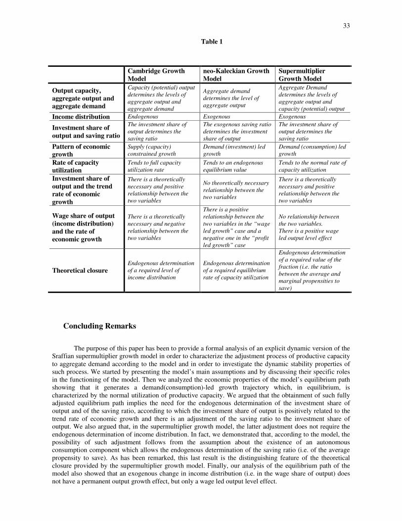
33

Table 1

Cambridge Growth

Model

neo-Kaleckian Growth

Model

Supermultiplier

Growth Model

Output capacity,

aggregate output and

aggregate demand

Capacity (potential) output

determines the levels of

aggregate output and

aggregate demand

Aggregate demand

determines the level of

aggregate output

Aggregate Demand

determines the levels of

aggregate output and

capacity (potential) output

Income distribution Endogenous Exogenous Exogenous

Investment share of

output and saving ratio

The investment share of

output determines the

saving ratio

The exogenous saving ratio

determines the investment

share of output

The investment share of

output determines the

saving ratio

Pattern of economic

growth

Supply (capacity)

constrained growth

Demand (investment) led

growth

Demand (consumption) led

growth

Rate of capacity

utilization

Tends to full capacity

utilization rate

Tends to an endogenous

equilibrium value

Tends to the normal rate of

capacity utilization

Investment share of

output and the trend

rate of economic

growth

There is a theoretically

necessary and positive

relationship between the

two variables

No theoretically necessary

relationship between the

two variables

There is a theoretically

necessary and positive

relationship between the

two variables

Wage share of output

(income distribution)

and the rate of

economic growth

There is a theoretically

necessary and negative

relationship between the

two variables

There is a positive

relationship between the

two variables in the “wage

led growth” case and a

negative one in the “profit

led growth” case

No relationship between

the two variables.

There is a positive wage

led output level effect

Theoretical closure Endogenous determination

of a required level of

income distribution

Endogenous determination

of a required equilibrium

rate of capacity utilization

Endogenous determination

of a required value of the

fraction (i.e. the ratio

between the average and

marginal propensities to

save)

Concluding Remarks

The purpose of this paper has been to provide a formal analysis of an explicit dynamic version of the

Sraffian supermultiplier growth model in order to characterize the adjustment process of productive capacity

to aggregate demand according to the model and in order to investigate the dynamic stability properties of

such process. We started by presenting the model’s main assumptions and by discussing their specific roles

in the functioning of the model. Then we analyzed the economic properties of the model’s equilibrium path

showing that it generates a demand(consumption)-led growth trajectory which, in equilibrium, is

characterized by the normal utilization of productive capacity. We argued that the obtainment of such fully

adjusted equilibrium path implies the need for the endogenous determination of the investment share of

output and of the saving ratio, according to which the investment share of output is positively related to the

trend rate of economic growth and there is an adjustment of the saving ratio to the investment share of

output. We also argued that, in the supermultiplier growth model, the latter adjustment does not require the

endogenous determination of income distribution. In fact, we demonstrated that, according to the model, the

possibility of such adjustment follows from the assumption about the existence of an autonomous

consumption component which allows the endogenous determination of the saving ratio (i.e. of the average

propensity to save). As has been remarked, this last result is the distinguishing feature of the theoretical

closure provided by the supermultiplier growth model. Finally, our analysis of the equilibrium path of the

model also showed that an exogenous change in income distribution (i.e. in the wage share of output) does

not have a permanent output growth effect, but only a wage led output level effect.

34

In the sequence, we undertook a formal analysis of the dynamic behavior of the model in the

neighborhood of its equilibrium point. First, we investigated the local dynamic stability properties of the

equilibrium path of the model. From such inquiry we obtained a local dynamic stability condition according

to which the model’s equilibrium is asymptotically stable if the expanded marginal propensity to spend has a

value strictly lower than one in the neighborhood of the equilibrium point. We verified that if this stability

condition is met then a change in the rate of capacity utilization has a greater impact on the pace of capital

accumulation than on the rates of aggregate demand and output growth in the neighborhood of the

equilibrium point. Further, we established that from the stability condition it also follows that there exists a

maximum rate of economic growth below which a stable demand led growth process is viable. After the

investigation of the model’s stability, we undertook a qualitative analysis of its dynamic behavior in the

neighborhood of the equilibrium point. From such investigation we obtained a characterization of the

disequilibrium trajectories of the model’s stationary endogenous variables. This investigation revealed that,

if the stability condition is met then these trajectories display a cyclical and convergent pattern (i.e. the

equilibrium is a stable focus).

In the sequence, we used the results obtained in our analysis of supermultiplier growth model to

address the criticisms advanced against it. We argued that much of the criticisms are based on a misleading

representation and interpretation of the model according to which the supermultiplier model would be

required to generate continuously fully adjusted growth paths. Clearly, in this case, the model would not be a

plausible explanation for economic growth as demand-led process. However, we pointed out that the model

used to represent the supermultiplier model is in fact a formalization of the economic growth process based

on Say’s Law. Thus, this model could not be a good representation of a model whose main objective is to

extend the applicability of the principle of effective demand to the analysis of the long run economic growth

process. In contrast, our analysis of the of the supermultiplier model demonstrated that the model produces

growth trajectories in which aggregate demand determines aggregate output. It showed, as well, that the

model does not generate continuously fully adjusted paths, in the sense that, outside the equilibrium path, the

growth trajectories produced by the model are featured by the divergence of the actual rate of capacity

utilization from its normal level. Actually, in this respect, we argued that such divergence is an essential

element in the characterization of the adjustment process of productive capacity to aggregate demand

according to the supermultiplier growth model. Thus, against the critics’ opinion, our analysis has

demonstrated that in the latter model the expansion of aggregate demand has a determining role in the

process of economic growth and that this determining role is fully compatible with the tendency towards the

normal utilization of productive capacity. Further, we also argued that the validity of model’s conclusions

does not require the exact equality between the time average of the actual rates of capacity utilization and the

normal rate of capacity utilization. We asserted that such requirement is excessively strong and not needed,

and, therefore, that the imposition of such requirement to the supermultiplier model is a kind of misplaced

exigency of precision on the part of some of the model’s critics. Finally, we addressed the criticism

according to which the existence of the tendency towards normal capacity utilization would require hyper-

rational behavioral assumptions in individual capitalist investment decisions and that it would be impaired by

the influence of the process of adjustment of capacity to demand on aggregate investment as a component of

aggregate demand. In this connection, we argued that no such hyper-rational behavioral assumptions are

needed according to our analysis of the adjustment process of capacity to demand based on the

supermultiplier growth model. We also showed that the effect of the adjustment process of capacity to

demand on aggregate investment as a component of aggregate demand is already considered in our analysis

of the stability of the model’s equilibrium path. Therefore, we argued that if the stability condition presented

in this paper is met the latter effect is not an obstacle to the prevalence of the tendency towards normal

capacity utilization.

In the last section of the paper we compared the supermultiplier, Cambridge and neo-Kaleckian

growth models pointing out their main similarities and differences as summarized in Table 1. The most

important conclusion obtained from the comparative analysis is that the supermultiplier growth model

provides an alternative heterodox explanation for the relationship between economic growth, income

distribution and effective demand. Such explanation does not involve, as in the case of the neo-Kaleckian

growth models, the endogenous determination of an equilibrium (long run) rate of capacity utilization that

must be able to assume very high or low values and, hence, can permanently diverge from its normal (or

planned) level. Moreover, such explanation does not depend on an endogenous determination of income

distribution that implies the existence of a theoretically necessary a priori relationship between income

35

distribution and economic growth, as we can find in growth models based on the Cambridge theory of

income distribution. In fact, the alternative theoretical closure provided by the supermultiplier growth model

enables a demand-led interpretation of the growth process that is compatible with a tendency towards normal

utilization of productive capacity and with a determination of income distribution from outside the model by

political, historical and economic forces. Therefore, the supermultiplier growth model provides a true

alternative to the Cambridge and neo-Kaleckian growth models in the analysis of the relationship between

economic growth, income distribution and effective demand. An alternative that has not yet been much

explored as the Cambridge and neo-Kaleckian ones, but that, we suggest, establishes a sound foundation for

a fruitful research program in heterodox economic growth theory

References

Allain, O. (2013) “Growth, Income Distribution and Autonomous Public Expenditures”, paper presented at

the 1st joint conference AHE - IIPPE - FAPE, Political Economy and the Outlook for Capitalism, Paris,

July 5-7, 2012.

Barbosa-Filho, N. H. (2000) “A Note on the Theory of Demand Led Growth”, Contributions to Political

Economy, vol. 19, pp. 19-32.

Bhaduri, A. &Marglin, S. (1990) “Unemployment and the Real Wage: the economic basis for contesting

political ideologies”, Cambridge Journal of Economics, vol. 14, pp. 375 – 93.

Blecker, R. (2002) “Distribution, Demand and Growth in neo-Kaleckian Macro Models” in Setterfield, M.

(ed.) Demand-Led Growth: Challenging the Supply-side Vision of the Long Run, (Aldershot, Edward

Elgar).

Blomstrom, M., Lipsey, R. E. and Zejan, M. (1996), “Is Fixed Investment the Key to Economic Growth”,

The Quaterly Journal of Economics, Vol. 111, no. 1, pp. 269-276.

Bortis, H. (1979) Foreign Resources and Economic Development from Early Fifties to the Oil Crises:

consideration of some theoretical and empirical aspects, (Fribourg, Fribourg University Press).

Bortis, H. (1997) Institutions, Behavior and Economic Theory –A Contribution to the Classical-Keynesian

Political Economy, (Cambridge, Cambridge University Press).

Cesaratto, S., Serrano, F. &Stirati, A. (2003) “Technical Change, Effective Demand and Employment”,

Review of Political Economy, vol. 15, n. 1, pp. 33 - 52.

Chenery, H. B.: (1952), “Overcapacity and the acceleration principle”, Econometrica, vol. 20, no. 1, pp. 1–

28.

Ciccone, R. (1990)“Accumulation and Capacity Utilization: Some Critical Considerations on Joan

Robinson's Theory of Distribution”, in Bharadwaj, K. and Schefold, B. (eds.) Essays on PeiroSraffa,

(London, Unwin & Hyman).

DeLong, J. B. and Summers, L. (1991), “Equipment Investment and Economic Growth”, The Quaterly

Journal of Economics, Vol. 106, no. 2, pp. 445-502.

Duesenberry, J. S. (1956), “Innovation and growth”, American Economic Review, vol. 46, no. 2, pp. 134–

141.

Dutt, A. K. (1984). “Stagnation, income distribution and monopoly power”, Cambridge Journal of

Economics, Vol. 8, no. 1, pp. 25 – 40.

Dutt, A. (1990) Growth, Distribution and Uneven Development, (Cambridge, Cambridge University Press).

Dutt, A. K. (2011) “The role of aggregate demand in classical-Marxian models of economic growth”,

Cambridge Journal of Economics, 35, pp. 357-82.

Ferguson, B. S. & Lim, G. C. (1998) Introduction to Dynamic Economic Models, (Manchester, Manchester

University Press).

Freitas, F. (2002) Uma Análise da Evolução das Ideias de Kaldor sobre o Processo de Crescimento

Econômico, Unpublished PhD Thesis, Federal University of Rio de Janeiro, Rio de Janeiro.

36

Freitas, F. (2009) “O Papel da Teoria da Distribuição nos Modelos Crescimento com Pleno Emprego de

Kaldor: uma avaliação crítica”, mimeo, Ferderal University of Rio de Janeiro, Rio de Janeiro.

Freitas, F. & Dweck, E. (2010) “Matriz de Absorção de Investimento e Análise de Impactos Econômicos”, in

Kupfer, D., Laplane, M. F. &Hiratuka, C. (Coords.) Perspectivas de Investimento no Brasil: temas

transversais, (Rio de Janeiro, Synergia).

Freitas, F. & Dweck, E. (2013) “The Pattern of Economic Growth of the Brazilian Economy 1970-2005”, in

Levrero, S., Palumbo, A. & Stirati, A. (eds.) Sraffa and the Reconstruction of Economic Theory,

volume II: aggregate demand, policy analysis and growth, (London, Palgrave Macmillan),

forthcoming.

Gandolfo, G. (1997) Economic Dynamics, (Heidelberg, Springer-Verlag).

Garegnani, P. (1992) “Some notes for an analysis of accumulation”, in Halevi, J. Laibman, D. & Nell, E.

(eds.) Beyond the Steady State: a Revival of Growth Theory (London, Macmillan).

Goodwin, R. (1951), “The nonlinear accelerator and the persistence of business cycles”, Econometrica, vol.

19, n. 1, pp. 1–17.

Harrod, R. (1939), “An Essay in Dynamic Theory”, The Economic Journal, Vol. 49, No. 193, pp. 14-33.

Harrod, R. (1948), Towards Economic Dynamics: Some Recent Developments of Economic Theory and their

Application to Policy (London, Macmillan)

Hein, E., Lavoie, M. & van Treeck, T. (2012) “Harrodian Instabilty and the ‘Normal Rate’ of Capacity

Utilization in neo-Kaleckian Models of Distribution and Growth – a survey”, Metroeconomica, vol.

63, n. 1, pp. 139-69.

Hicks, J. R. (1950) A Contribution to the Theory of the Trade Cycle, (Oxford, Clarendon Press).

Kaldor, N. (1955-6[1960a]) “Alternative Theories of Distribution”, in Kaldor, N., Essays on Value and

Distribution, (Glencoe-Illinois, Free Press).

Kaldor, N. (1951), “Mr Hicks on Trade Cycle”, The Economic Journal, Vol. 61, No. 244, pp. 833-847.

Kaldor, N. (1957[1960b]) “A Model of Economic Growth”, inKaldor, N., Essays on Economic Stability and

Growth, (Glencoe-Illinois, Free Press).

Kaldor, N. (1958[1978]). “Capital Accumulation and Economic Growth”, in Kaldor, N., Further Essays on

Economic Theory, (N. York, Holmes & Meier).

Kaldor, N. (1962[1978]). “A New Model of Economic Growth”, in Kaldor, N., Further Essays on Economic

Theory, (N. York, Holmes & Meier).

Kalecki, M. (1971) Selected Essays on the Dynamics of Capitalist Economy 1933 – 1970, (Cambridge,

Cambridge University Press).

Koyck, L.: (1954), Distributed lags and Investment Analysis, (Amsterdam, North Holland).

Kurz, H. D. (1990) “Accumulation, distribution and the 'Keynesian Hypothesis’”, in Bharadwaj, K. and

Schefold, B. (eds.) Essays on Peiro Sraffa, (London, Unwin & Hyman).

Lavoie, M. (1992) Foundations of Post-Keynesian Economic Analysis, (Aldershot, Edward Elgar).

Medeiros, C. & Serrano, F. (2001) "Inserção externa, exportações e crescimento no Brasil" in Fiori, J. &

Medeiros, C. (orgs.) Polarização Mundial e Crescimento, (Petrópolis, Vozes).

Marglin, S. A. & Bhaduri, A. (1990) “Profit Squeeze and Keynesian Theory”, in Marglin, S. A.& Schor, J.

B. (eds.) The Golden Age of Capitalism, (Oxford, Oxford University Press)

Palumbo, A. (2009) “Adjusting Theory to Reality: The Role of Aggregate Demand in Kaldor's Late

Contributions on Economic Growth”, Review of Political Economy, Vol. 21, No. 3, pp. 341-368.

Park, M.-S.(2000), “Autonomous Demand and Warranted Rate of Growth”, Contributions to political

Economy, vol. 19, pp. 1-18.

37

Robinson, J. (1962) Essays on the Theory of Economic Growth, (London, Macmillan).

Rowthorn, B. (1981): ‘Demand, real wages and economic growth’, Thames Papers in Political Economy,

Autumn, pp. 1–39.

Sala-i-Martin, X. (1997) “I Just Ran Two Million Regressions”, American Economic Review, Papers and

Proceedings of the Hundred and Fourth Annual Meeting of the American Economic Association, Vol.

87, no. 2, pp. 178-183.

Schefold, B. (2000) “Fasi dell’accumulazione e mutevoli influenze sulla distribuizione”, in Pivetti, M. (ed.)

Piero Sraffa: contributti per unabiografia intellettuale, (Rome, Carocci).

Serrano, F. (1996) The Sraffian Supermultiplier, Unpublished PhD Thesis, Cambridge University, UK.

Serrano, F. (1995). “Long Period Effective Demand and the Sraffian Supermultiplier”, Contributions to

Political Economy, vol. 14, pp. 67-90.

Serrano, F. & Freitas, F. (2007) “El Supermultiplicador Sraffiano y el Papel de la Demanda Efectiva em los

Modelos de Crecimiento”. Circus, vol. 1, pp. 19-35

Serrano, F. &Wilcox, D. (2000). “O modelo de dois hiatos e o supermultiplicador”, Revista de Economia

Contemporânea, vol. 4, n. 2, pp. 37 – 64.

Skott, P. (2008) “Theoretical and empirical shortcomings of the neo-Kaleckian investment function”,

Working paper, University of Massachusetts, Amherst.

Steindl, J. (1952) Maturity and Stagnation in American Capitalism, (Oxford: Basil Blackwell).

Steindl, J. (1979) “Stagnation Theory and Stagnation Policy”, Cambridge Journal of Economics, vol. 3, n. 1,

pp. 1-14.

Steindl, J. (1982), “The role of household saving in the modern economy”, Banca Nazionale del Lavoro

Quarterly Review, vol. 35, n.140, pp. 69–88.

Trezzini, A. (1995), “Capacity Utilization in the Long Run and the Autonomous Components of Aggregate

Demand”, Contributions to Political Economy, vol. 14, pp. 33-66.

Trezzini, A. (1998) “Capacity Utilization in the Long Run: some further considerations”, Contributions to

Political Economy, vol. 17, pp. 53-67.

Vianello, F. (1989), “Natural (or Normal) Prices. Some Pointers”, Political Economy. Studies in the Surplus

Approach, vol. 5, No. 2, pp. 89–105.

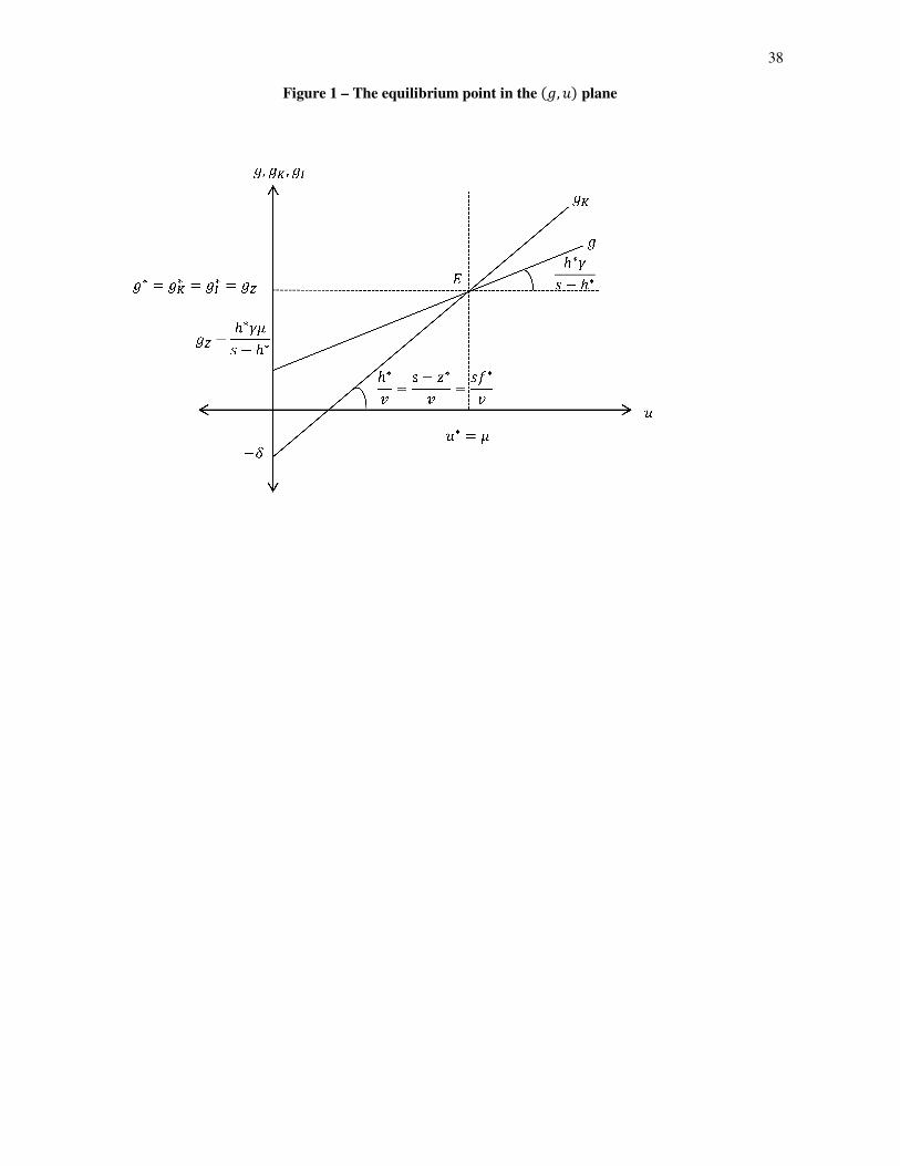
38

Figure 1 – The equilibrium point in the ��, �� plane

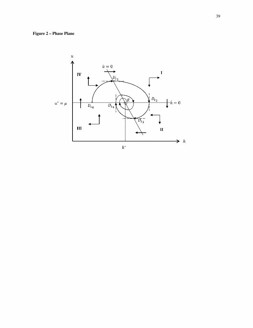
39

Figure 2 – Phase Plane

40

Figure 3

IV I II III

IV I II III

41

Figure 4

IV I II III

,

IV I II III

42

Figure 5

43

Figure 6

iProfessor at the Institute of Economics of the Federal University of Rio de Janeiro.Address: Instituto de

Economia/UFRJ, Av. Pasteur, 250, Urca, Rio de Janeiro, RJ, 22.290-240. Phone: 55 21 3873-5242. Fax: 55 21 2541-

8148. Contact: fabio@ie.ufrj.br.

ii Professor at the Institute of Economics of the Federal University of Rio de Janeiro. Address: Instituto de

Economia/UFRJ, Av. Pasteur, 250, Urca, Rio de Janeiro, RJ, 22.290-240. Phone: 55 21 3873-5242. Fax: 55 21 2541-

8148. Contact: franklin.serrano@gmail.com.