Economic Research Southern Africa (ERSA) is a research programme funded by the National

Treasury of South Africa. The views expressed are those of the author(s) and do not necessarily represent those of the funder, ERSA or the author’s affiliated

institution(s). ERSA shall not be liable to any person for inaccurate information or opinions contained herein.

Growth (and Segregation) by Rail: How the

Railways Shaped Colonial South Africa

Johan Fourie and Alfonso Herranz-Loncan

ERSA working paper 538

August 2015

Growth (and Segregation) by Rail: How theRailways Shaped Colonial South Africa¤

Johan Fourieyand Alfonso Herranz-Loncanz

August 25, 2015

Abstract

The railway played a large part in late nineteenth century and earlytwentieth century globalization since, to bene…t from the internationaleconomy, peripheral countries needed cheap inland transport. This pa-per discusses how the railway transformed the economy of South Africa’sCape Colony during the …rst era of globalization. A very large share ofthe Colony’s GDP came from rail transport – its resource saving e¤ectwas one of the highest in the world at that time. We estimate that 46to 51% of the Colony’s increase in labor productivity between 1873 and1905 came directly from the railway, whether from investment in the railnetwork or from savings in transport costs. We argue that it was theboom in diamond production, necessitating the building of the railwayto connect the Kimberley diamond …elds with the international economy,that weighted the Colony’s economy so heavily towards the rail trans-port sector. The railway not only boosted the Colony’s growth, it alsore-shaped its economic geography, organizing it around the railway linesthat connected the diamond mines with the ports. Areas not served by therailway missed out on the bene…ts of globalization. As these areas weremostly populated by blacks, the railway helped to create a dual economywith a racial social divide and was later instrumental in creating black‘homelands’ and establishing the apartheid institutions.

JEL CODES: N4, H4, OKey words — railways, Cape Colony, South Africa, social savings,

economic geography, segregation

¤We would like to thank Dan Bogart, Latika Chaudhary, Remi Jedwab, Edward Kerby,Martine Mariotti, Anne McCants, Alexander Moradi, John Tang, Jan Greyling, Nonso Obikili,Dieter von Fintel and participants at the World Economic History Congress 2015, at the Centrefor Economic History Workshop at ANU, and the 12th ERSA Economic History Workshop inCape Town for valuable feedback on an earlier version of this paper.

yDepartment of Economics, Stellenbosch University, South Africa. E-mail: jo-hanf@sun.ac.za

zDepartment of Economic History and Institutions, University of Barcelona, Spain. E-mail:alfonso.herranz@ub.edu

1

1 INTRODUCTIONThe railway was a powerful force driving late nineteenth century globalization.Across the periphery, and due to the scarcity of previous transport infrastruc-ture, in the absence of railways the e¤ects of globalization were evident only innarrow strips of land along the coasts or close to navigable rivers. The railwaywas more vital for economic growth in the periphery than in the industrializedcountries, which already had good transport infrastructure and well-integratedmarkets at the beginning of the railway era. Railways were essential for thee¤ects of globalization to penetrate a periphery country’s hinterland, and thetracks would shape its economic geography, with e¤ects that in some cases livedon after the railway ceased to operate.

Railway construction was, however, not spread evenly throughout the pe-ripheral countries. In Latin America the density of the railway networks variedwidely from country to country (Bignon et al., 2015). Argentina’s network in1913, for example, was 12 and 25 times larger than Columbia’s per sq. kmof surface area and per capita. Unsurprisingly, these two countries also hadsubstantially di¤erent levels of integration into the international economy andincome per capita. Variations in railway density were even more marked in sub-Saharan Africa because of huge di¤erences in ruggedness, climate, natural en-dowments or institutions (such as the timing and type of colonization). Whereasin southern Africa colonial governments in the late nineteenth and early twenti-eth century constructed a complex system of interconnected railway networks,other sub-Saharan African colonial territories had only some unconnected lineslinking the main ports with a few interior production areas or cities.1 As in otherregions of the world, the economic e¤ects of globalization followed the railwaytracks inland into sub-Saharan Africa. These e¤ects were felt most strongly inthe regions with the larger and denser railway networks.

In this paper we discuss the way the railway transformed the economy of theCape Colony during the late nineteenth and early twentieth century globaliza-tion, from the early 1870s to 1905. The Cape’s railway network has always been(together with the rest of the South African network) the largest and densestin sub-Saharan Africa. In addition, before 1910 the Cape Colony’s rail trans-port sector accounted for a surprisingly high share of GDP. The cost savinge¤ect of a mode of transport depends on two factors: the cost advantage overthe next best alternative, and the amount of freight and number of passengerstransported. The Cape was not particularly notable for the cost advantage ofrail transport (compared with that of other African countries that had to relyon head porterage where there were no railways), but its rail tra¢c reached alevel unequalled by many other peripheral countries. The resource saving e¤ectof its railway network was one of the highest in the world at that time.

1By 1910, 45% of sub-Saharan Africa’s railway lines were in the Union of South Africa.The railway lines in Portuguese East Africa, South West Africa, Northern Rhodesia, SouthernRhodesia and the Union of South Africa (now Mozambique, Namibia, Zambia, Zimbabwe andthe Republic of South Africa) together made up 67% of the region’s railway network (Mitchell,(2003a).

2

We argue that it was because of the boom in diamond production that theColony’s economy was so heavily weighted towards rail transport. The Caperailways were built to connect Kimberley with the international economy and toallow Kimberley’s economy to boost and increase its population. By reducingthe cost of transport to the interior, the railway eased the movement of labor,capital goods, foodstu¤s and other necessities to the diamond mining centersand transformed the Cape from a traditional agrarian economy to a diamondexporting power and a center of attraction for immigrants. Its real GDP grew ata yearly rate of 4.77% between 1870 and 1909 (Greyling and Verhoef, 2015). Thecentrality of the railway in that process is re‡ected in our estimation that 46 to51% of the Colony’s increase in labor productivity between 1873 and 1905 camedirectly from the railway, either from investment in the rail network or fromthe cost-saving e¤ects of rail transport. This is a very high share for a singlesector and clearly indicates the transformative power of the new infrastructure.To a large extent, economic growth in the Cape during the …rst globalizationwas made possible by the railway.

A similar process took place a few years later on a larger scale with goldproduction in the Transvaal. Thus, in the Cape and in the whole Union ofSouth Africa,2 the railway was crucial for connecting the international econ-omy with the mining areas, enabling the expansion of mining production andthe development of some of the most important industrial and urban hubs inAfrica. Naturally, as in other countries (Jedwab and Moradi, 2015; Jedwabet al., 2014), it also helped to shape the economic geography, which was orga-nized around the routes that connected the main ports with the mining centers,leaving large areas almost untouched by the new transport technology and com-paratively isolated. Nowhere was this more evident than in the Transkei andBasutoland3 which, despite being fairly close to the Kimberley district, couldneither become its suppliers nor bene…t from the diamond boom. Since theseisolated areas were populated mostly by blacks, the reorganization of the Cape’seconomic geography had an evident racial bias. Thus, although the exclusionof Basutoland or the Transkei can be largely explained by the ruggedness of theterrain and previous history of resistance to the colonial government, it endedup creating a dual economy with a clear racial component and contributing tothe segregation policies of the twentieth century.

The Cape Colony was one of the countries most a¤ected by the coming ofthe railway. The railway was vital for the growth of the Colony’s economy andplayed a large part in shaping its economic geography and eventually that ofSouth Africa. But it also played a large part in the segregation of territoriesand the establishment of apartheid, going hand in hand with the colonial insti-tutions that prevented blacks from enjoying the income-earning opportunitiesof globalization.

2The four British colonies, the Cape Colony, Natal Colony, Transvaal Colony and OrangeRiver Colony, became the Union of South Africa in May 1910.

3The Transkei is now incorporated into the Eastern Cape province and Basutoland is nowLesotho.

3

2 THE RAILWAYS OF THE CAPERailway construction in the Cape Colony started in 1859, but progress was slowuntil the early 1870s, with the only line in operation being the 57-mile routebetween Cape Town, Wynberg and Wellington. The government acquired thisrailway in 1872, only a few years after the discovery of diamonds in the Kim-berley area in 1866, and from then on the construction and operation of thenetwork remained a public undertaking in the hands of the Cape GovernmentRailways (CGR).4 As a consequence of the diamond rush and, later, the discov-ery of gold in the Witwatersrand Basin in 1886, railway construction acceleratedrapidly. By 1910, when the CGR ceased to exist as a separate company andwere incorporated into the administration of the Union Government Railways,the network had reached a length of more than 3,300 miles.

The Cape Colony’s railway network initially consisted of three trunk linesconnecting the ports of Cape Town, East London and Port Elizabeth with theinterior of the country and the diamond producing area. The network wasgradually enlarged with numerous branch lines and by 1910, together with therailways of the Transvaal and the Orange Free State, this was by far the largestand densest railway network in Africa, both per sq. km of surface area and percapita, and one of the largest networks outside Europe and the US. Figure 1shows how fast the Cape Colony’s railway network grew and Table 1 comparesit with those of other countries.

Figure 1 shows that before 1910 there were two main periods of railwayconstruction in the Cape Colony. The …rst took place between 1875 and 1885,the years of the construction of the main trunk line linking Cape Town andKimberley, and the two routes connecting this line with Port Elizabeth andEast London. The second took place in the …rst years of the twentieth century,just after the end of the second Anglo-Boer War, and investment was thenconcentrated on branch lines that might act as feeders to the trunk lines oras connections between them (such as those on the route between Cape Townand Port Elizabeth), and on extending the main trunk line farther away fromKimberley through the border of the Cape Colony, providing a route to thegold-producing areas of the Transvaal which was also part of the Cape-to-Cairorailway and river transport project. The construction of branch lines continuedthrough the late 1920s, bringing the total network length to over 5,000 miles.

Like the railways of other resource exporting countries, those of the CapeColony were used mainly to carry freight, although passenger tra¢c was alsosizeable, amounting to almost one-third of total revenues (Figure 2). Table 2shows the average composition of freight tra¢c between 1903 and 1908, withthe biggest categories of freight being general products, agricultural goods, andcoal and coke, largely re‡ecting the role of the railway as supplier of the miningproduction areas in the interior of the country.5

4The only exception was a narrow-gauge mining railway that was built in Namaqualandin the late 1860s and linked the copper mines in the O’Okiep area with the sea. This railwaywas initially horse-drawn and gradually adapted to steam. The line was closed in 1945.

5For the correspondence between the transport of general products and imports to the

4

From 1873 to 1908 the Colony’s railway tra¢c kept pace with the cycle of di-amond mining production in the Kimberley area. Tra¢c began to decrease onlyin 1905, when international competition caused a crisis in the diamond market.During the diamond boom, rail freight transport accounted for an exceptionallyhigh share of the Cape GDP (Figure 3). Even leaving aside the 1900–1902 peak,which was the result of increasing transport requirements associated with thesecond Anglo-Boer War, we can see that the railway’s GDP share is huge –much larger than that of most other countries at the time.

Nevertheless, despite the sharp increase in tra¢c, the CGR’s …nancial re-turns were barely su¢cient to cover the opportunity cost of capital. Between1873 and 1908 net returns comprised on average just 3.7% of the accumulatedcapital. Even during the period of highest tra¢c, returns remained below 5%,with the exception of six years (Figure 4). By comparison, the interest ratesof the railway bonds and most Cape Government debt issues were set at 3.5 or4%.6 Given that net returns should be su¢cient to cover both the amortiza-tion of equipment and infrastructure and the opportunity cost of capital, anyreturn below 5% must have been too low to make the Cape Colony railways asource of net revenue for the government. By contrast, and given the size ofthe rail transport sector (Figure 3), the bene…ts that accrued to the users weresubstantial, as is shown in the next section.

3 THE CONTRIBUTION OF THE CAPE COLONYRAILWAYS TO ECONOMIC GROWTH

In this section we assess the contribution of the railway to the growth of theColony’s economy between 1873 (just before the …rst period of expansion of thenetwork) and 1905 (the last year before the start of the crisis in the diamondmining economy) using the growth accounting method.7 Our measurement ofthe growth contribution derives from the transformation of the usual Solowexpression for increases in labor productivity:

¢(Y /L)/(Y /L) = sK¢(K/L)/(K/L) + ¢A/A (1)

where Y is total output, L is the total number of hours worked, K representsthe services provided by the physical capital stock, Ais total factor productiv-ity (TFP), and sK is the factor income share of physical capital. The growthcontribution of a new technology (measured as the sum of disembodied TFPgrowth and the embodied capital-deepening e¤ect of investment in that tech-nology) can be calculated by distinguishing, in expression (1), between di¤erent

mining districts, see for instance the Report of the General Manager of Railways for the year1905, (Cape of Good Hope Government 1906: 3).

6Cape of Good Hope Government (1900-1909) Statistical Register of the Colony of theCape of Good Hope, 1903.

7For a summary of the growth accounting method for estimating the direct contributionof a new technology to economic growth, see for instance Oliner and Sichel (2002), Crafts(2004b) or Herranz-Loncán (2011, 2014).

5

types of capital and di¤erent components of TFP growth:

¢(Y/L)/(Y/L) = sKo¢(Ko/L)/(Ko/L) + γ(¢A/A)o

+sKNT ¢(KNT /L)/(KNT /L) + φ(¢A/A)NT (2)

where KNT and Ko are capital services in the new technology and in othersectors, respectively, A is the TFP level in the sector indicated by the subscript,sKNT and sKo are the factor income shares of the capital invested in the newtechnology and other capital, and φand γare the shares of the new technologyand other sectors’ production in total output. The growth contribution of thenew technology may be measured as the sum of the last two terms of equation(2), which represent, respectively, the capital term and the TFP term of thatcontribution.

The calculation of the capital term is straightforward on the basis of railwayaccounting data. As for the TFP term, according to the price dual measureof productivity, the TFP contribution of the railway would be equivalent tothe direct real income gain obtained from the reducing the resource cost oftransport. Under perfect competition, this would be captured by the equivalentvariation in consumer surplus associated to the use of the railway.8 This requirescomparing the price of rail transport at the end of the period under consideration(1905) with the price of other forms of Cape inland transport just before theintroduction of the railway to the Cape economy (1873). As suggested in Crafts(2004a), Leunig (2010) and Herranz-Loncán (2014), this exercise is similar tomeasuring the social saving of railways, which is usually calculated as:

SS = (PALT ¡ ¡PRW )xQRW (3)

where PRW and PALT are, respectively, the cost of rail and alternative trans-port, and QRW is the rail transport output in the reference year. The socialsaving is thus an upward-biased estimate (due to the implicit assumption of aprice-inelastic transport demand) of the equivalent variation in consumer sur-plus provided by the railway, and correcting it for the elasticity of demand andadding the potential supernormal pro…ts of the railway companies would providea measure of the TFP term of the railway’s growth contribution.9

8The possible presence of imperfect competition or scale economies in the transport-usingsectors makes this measure a lower bound estimate of the total income gain of the railways,due to the exclusion of TFP spillovers, a problem that must be kept in mind in interpretingthe results.

9There is, however, an important di¤erence between the objectives of growth accountingand the social saving exercises. The estimation of the growth contribution of the railway doesnot involve any counterfactual consideration, but is a pure accounting exercise, which aims atidentifying the sources of the actual economic growth. By contrast, the social saving aims atanalysing how the economy would have looked like without the railway. The latter, therefore,may allow for adjustments in the non-railway counterfactual economy (improved road or canalinfrastructure, for instance) which are not considered in the former, which uses as input theactual situation of the transport sector before the introduction of the railway.

6

3.1 The capital term

To estimate the capital term of the growth contribution of the railways, we…rst measure the per capita growth rate of the accumulated capital investedin the network, as published in the successive Reports of the General Managerof Railways (Cape of Good Hope Government, 1873-1909), and after de‡atingthe yearly di¤erences in the capital account by the price index for the CapeColony (Verhoef et al., 2014).10 The resulting per capita yearly rate is 4.52%,very similar to the growth rate of the network length (4.39%).11 As may be seenin equation (2) above, that rate must be multiplied by the factor income shareof railway capital, i.e. the average ratio of railway net revenues to nominal GDPfrom 1873 to 1905. We estimate this ratio to be 3.32%, a fairly high …gure.12

The product of the capital per capita growth rate and the capital income shareis 0.15%. This percentage represents the capital term of the growth contributionof the Cape Colony railway, i.e. the percentage points of growth of the economythat resulted from the embodied capital-deepening e¤ect of investment in therailway.

3.2 The TFP term

Our calculations of the TFP term are based, as has been indicated, on an estima-tion of the social saving provided by the railway, which must be corrected for theelasticity of demand.13 This requires information on the amount of freight andnumber of passengers transported by the railway in the …nal year of the analysis(1905), the unit price of rail transport in 1905, the unit price of pre-rail trans-port, and the price elasticity of (freight and passenger) transport demand.14

The next two subsections provide estimates of these magnitudes and the result-ing TFP term of the growth contribution of the Cape Colony railways between

10The yearly population of the colony is estimated by a log interpolation between census…gures, taken from Union of South Africa (1919).

11The amount of capital invested in the network would grow faster than the network lengthif improvements were made to the lines, such as double tracks, substitution of steel for iron,etc. However, this e¤ect could be partially overcome if the new branch lines were of lowerunit construction cost than the trunk lines.

12This …gure is the average over 1873–1905 of the yearly ratios between the net returnsof the railways taken from the Report of the General Manager of Railways (Cape of GoodHope Government, 1873-1909) and the nominal GDP calculated by Verhoef et al. (2014).The equivalent …gure for the UK between 1850 and 1910 would be 2.52% and for Argentinabetween 1865 and 1913, 1.81%; see Crafts (2004b) and Herranz-Loncán (2014).

13As indicated before (footnote 11), we use a restricted concept of social saving, that ex-cludes improvements in the alternative transport means in the absence of railways.

14This estimation procedure makes the TFP term very sensitive to the situation in the …naldate of the analysis. We chose 1905 because we aimed to capture the whole contribution ofthe railway technology to the Cape Colony’s economic growth before its incorporation into theUnion of South Africa in 1910. This contribution was complete by 1905, when the maximumpotential use of the network was reached (we ignore the exceptionally high levels of tra¢c of1902–1903, which were a consequence of the war). Choosing a year of crisis in the miningeconomy (such as any year between 1906 and 1908) would bias our estimates downward,reducing our estimates by approximately half.

7

1873 and 1905.15

3.2.1 Freight tra¢c

In 1905 the CGR transported approximately 361 million ton-miles of freight,each one of which ran an average of 197 miles and was charged a unit averagerate of 1.55 pence.16 To calculate the social saving provided by the railway, weassume that, in the absence of the railway, all this freight would have been movedby road.17 Our main evidence of road transport prices comes from di¤erencesin 1890 between the prices of four agricultural products (barley, maize, oat hayand wheat) in three South African cities that were not connected by rail inthat year (Kimberley, Johannesburg and Bloemfontein).18 Although di¤erencesbetween product prices (especially in the two cities that were closest together,Kimberley and Bloemfontein) do not allow for a very precise estimation, theywould be consistent with a structure of road transport prices that, as would beexpected, decreased with distance. They are also consistent with some scatteredinformation on road transport costs in the Report of the General Manager ofRailways, which the company used to analyze how much competition the ox-wagon still represented in the early twentieth century (Cape of Good HopeGovernment, 1873-1909). For instance, in the Report for 1906 (p. ix), a price of29 pence is quoted for the ox-wagon transport of 100 lb (pounds) of general goodsfrom Port Elizabeth to Grahamstown, which would be equivalent to £0.033(pounds sterling of 1905) per ton-mile over a distance of 80 miles. Rhind (1995)and Pirie (1993) also supply some evidence of the prices charged by ox-wagoncarriers in various areas of the Cape.19 If we adjust all these observations to alog cost function of distance (see Figure 5), and apply the estimated function tothe average distance traveled by freight through the rail network in 1905 (197miles), the resulting rate for the ox-wagon transport is £0.021 per ton-mile, i.e.

15The TFP term should be increased by the amount of extraordinary pro…ts (over theopportunity cost of capital) that accrued to the railway …rms. However, as has been indicatedabove, those pro…ts were probably negligible or slightly negative during the period understudy, since net returns amounted on average to 3.7% of the accumulated investment. Wetherefore omit them from our estimation.

16Figures estimated from information in the Report of the General Manager of Railwaysfor 1905. Due to the lack of information, we exclude from the calculation the transport oflivestock, vehicles and parcels transported at high-speed, which amounted to approximately12% of the total revenues of (low and high-speed) freight transport between 1891 and 1908.

17Due to insu¢cient information, we cannot take into account the possibility of some railwaytra¢c taking place between ports, where goods could have moved by boat in an economywithout railways. This could introduce an upward bias in the estimation, since water transportprices were much lower than carting rates per ton-mile. However, we assume the size of thisbias to be small since, as has been indicated, the railways were designed mainly to carryfreight from the port cities to the consumer areas in the interior.

18Our agricultural price data come from several issues of the Agricultural Journal, publishedby the Department of Agriculture of the Cape Colony. The Journal provides monthly prices;we use the average over the 12 months of the year 1890.

19The prices, in pounds sterling of 1905 per ton-mile, are £0.024 between Robertson andWorcester (30 miles); £0.026 between Port Elizabeth and Humansdorp (54 miles); and £0.013between East London and Elliot (155 miles). For the …rst observation see Rhind (1995: 13);for the other two see Pirie (1993: 324–325).

8

3.3 times the average rail freight cost of £0.0065.Table 3 shows that the social saving of freight transport in the Cape Colony

amounted to approximately 13% of the Colony’s GDP in 1905. Table 4 comparesthis saving with available estimates for other countries and shows the size of eachcountry’s railway sector and the di¤erence between the cost of rail and pre-railfreight transport in each country. As may be seen in the table, the freight socialsaving in the Cape Colony was lower than that of other primary exportingcountries that also built dense railway networks during the …rst globalization,such as Mexico or Argentina, but higher than that of other sub-Saharan Africancountries.20 The Colony’s advantage over the latter may be explained entirelyby the very large size of the railway sector, since traditional road transport in theCape Colony seems to have been relatively competitive, compared not only withporterage (the usual transport method in other sub-Saharan African countries)but also with the cost of road transport in Latin American countries.21 Railfreight transport was the main source of the Cape’s resource savings, amountingto 5.5% of GDP in 1905.

To calculate the TFP term of the growth contribution of the railways, wetransform the social saving into an estimate of the additional consumer surplusof rail freight transport by correcting it for the price elasticity of transportdemand. Unfortunately, there is no information on unit prices and quantitiestransported by the CGR before 1903, and the sample of available observations(1903–1908) is too small to allow us to estimate a demand function. As asecond-best option, we use the set of elasticity estimates available for a numberof Latin American primary exporting countries in the same period, which rangefrom -0.5 to -0.8 (Herranz-Loncán, 2014). The estimates of additional consumersurplus of rail freight transport that result from applying these elasticities tothe social savings …gures are shown in Table 5.22

3.2.2 Passenger tra¢c

We must add to these an estimate of the additional consumer surplus of railpassenger transport, which should take into account people’s saving not onlyin cost but also in time, thanks to slower traditional transport being replacedby the railway. To calculate the time saving, we introduce some assumptionsabout the share of traveling time that should be deducted from the passengers’working time in the absence of railways, as well as their average hourly wage.

Given the lack of precise information on these factors, and following the

20However, Jedwab and Moradi (2015) provide much higher social saving estimates forGhana in 1931, amounting to 27% of GDP.

21On the competition between the railways and ox-wagon transport see Pirie (1993). Anexample of much more expensive road transport is the pre-rail transport of copper to the seain Namaqualand; see Ross (1998: 335). A possible source of downward bias in our estimateof road transport fares is the fact that most available evidence refers to grain, whereas higherprices may have been charged for transporting other goods (such as industrial products).

22The ratio of the additional consumer surplus to the social savings is given by [(ϕ1+ε-1)/(1-ε)(ϕ-1)], where ε is the absolute value of the elasticity of transport demand and ϕ isthe ratio of alternative to rail transport prices; see Fogel (1979: 10–11).

9

procedures applied in previous research on Latin America (Herranz-Loncán,2014), we base the estimation on the following assumptions: i) in the absenceof the railways, …rst-class passengers would have used stagecoach transport,but second and third class passengers would have used informal means, such ascarts, horseback or walking, ii) transport demand elasticity was approximately-1 in the case of the …rst class (since it was a transport mode with a certainluxury component); iii) in the absence of the railway all second and third classpassengers would still have traveled by some means, since they journeyed mainlyfrom necessity,23 iv) the value of the working travel time of second and thirdclass travelers can be calculated using the average hourly wage of wage-earners,and that of …rst-class travelers by the average hourly wage of skilled workers, andv) only about half of the time savings were savings in working time. The socialsavings and additional consumer surplus estimates that result from applyingthese assumptions to the rail transport of passengers in the Cape Colony arepresented in Tables 6 and 7.

The total social savings of passenger rail transport in the Cape Colonyamounted to 4.05% of GDP by 1905. While we recognize the signi…cant errormargin of this estimate,24 we note that the …gure is considerably higher thanthat of other primary exporting countries. For instance, in countries like Ar-gentina, Mexico or Brazil this percentage ranged from 2 to 4.4%, and in othersub-Saharan African countries it was negative (Chaves et al., 2013; Herranz-Loncán, 2014). When the social saving is transformed into additional consumersurplus by applying the aforementioned demand elasticities (-1 for the …rst classand 0 for the second and third classes) the resulting …gure is £1.1 million, i.e.2.5% of the GDP of the Colony. The aggregate additional consumer surplusof freight and passenger transport would therefore amount to 10.0% to 11.6%of GDP. This …gure would represent the total direct income gain of the CapeColony railways, and we use it as the TFP term in the growth contribution esti-mation by expressing it as percentage points of yearly growth during the period1873–1905. These are presented in Table 7, together with the capital term andthe whole growth contribution of the railways.

According to these estimates, 46 to 51% of the growth in labor productivityin the Cape Colony between 1873 and 1905 derived directly from the railway.Only about 20% of this impact was associated with capital-embodied techno-logical progress, while all the rest was a consequence of savings in transportcosts. This is a very high contribution for a single sector, much higher indeedthan the equivalent …gure for Britain or Spain, and comparable to the rail-ways’ contribution to labor productivity growth in Latin American countries(Herranz-Loncán, 2014). Moreover, this …gure excludes the indirect e¤ects of

23This is equivalent to assuming a null elasticity to the increasing cost of traveling.24The main possible source of bias in this estimate is the assumption of the same behaviour

for second and third class passengers. If second class passengers were assumed to behave as…rst-class ones (i.e. to use stagecoaches as alternative to railways) the social savings wouldincrease to 8.3% of GDP. The estimates are also highly sensitive to the level of the stagecoachrates, based on an insu¢ciently representative sample. Therefore, the …gures provided in thetable must be taken with caution.

10

the railway, such as the agglomeration economies arising from the urban con-centrations that the railway made possible. So, economic growth in the CapeColony during the …rst globalization seems to have been, to a signi…cant extent,a direct consequence of investment in railway infrastructure.

4 THE RAILWAY AND THE REORGANIZA-TION OF THE CAPE ECONOMY

As has been indicated, the main reason for constructing the Cape railwayswas to connect the Kimberly diamond producing district with the internationaleconomy. Unlike what happens with bulkier products, such as grain or coal,the very high value-to-weight ratio of diamonds meant that a cheap transportmethod was necessary not so much for shipping the product as for supplyingthe production area with industrial commodities, construction materials, fueland foodstu¤s. In other words, the construction of the railway was necessaryto enable the development of a dense population settlement around the mines.Thus, at least until the …rst few years of the twentieth century, the Cape railwaynetwork seems to have been used largely to supply the Kimberley district. Thecentrality of the diamond producing area within the railway network is re‡ectedin the fact that, apart from Cape Town, Port Elizabeth and East London, in1905 Kimberley was still by far the highest revenue generating station.25

Similarly, the Kimberley district, which by 1911 accounted for just 3.3% ofthe population of the Colony, was the destination of an extremely high percent-age of certain categories of rail freight. This is shown by the detailed tra¢cinformation by station and freight category that is provided by the Report ofthe General Manager of Railways for the year 1905, which makes it possible toidentify the districts that were net suppliers and net importers of each categoryof commodity. The Kimberley district had negative balances for almost all cat-egories, while its imports accounted for very high shares of the total imports ofthe Cape Colony districts with de…cit, such as 15% of general merchandise, 13%of grain of South African origin, 23% of other South African agricultural pro-duce, 44% of ‡our, meal, malt and bran of South African origin, 51% of SouthAfrican timber, 52% of …rewood, and an impressive 79% of South African coaland coke. Looking at these …gures another way, we …nd that per person in1905 the Kimberley district received, through the railways, 457 kg of cereals,‡our, meal, malt or bran, 14.5 kg of wine and spirits of South African origin,265 kg of other agricultural produce, and 354 kg of …rewood. These quantitiesdelivered by rail accounted for an exceedingly large share of the supply needsof the Kimberley population – clear evidence that the growth of the area waslargely based on the development of railway services.

The railway was responsible for an unprecedented increase in the scale of theCape inland transport. It thus removed restrictions to the growth of cities such

25Report of the General Manager of Railways for the year 1905 (Cape of Good HopeGovernment, 1873-1909).

11

as Kimberley (as it did some decades later with Johannesburg) and dramaticallyreduced the e¤ect of distance as a determinant of domestic trade ‡ows. Thegrowth of Kimberley thus no longer depended on the supplying capacity ofthe closer regions; rather, as our information on railway tra¢c shows, its mainsuppliers seem to have been either the port cities or the districts close to CapeTown, i.e. areas far away from the diamond production centers. Table 8 showsthe main suppliers of certain foodstu¤s in 1905 and the percentage of the totalinter-district railway deliveries they accounted for.

Although the available information does not provide the speci…c origins ofKimberley’s imports, all seems to indicate that Kimberly was provisioned withindustrial commodities and foodstu¤s that were either imported from othercountries or produced in the western part of the Colony – they did not comefrom the (much closer) eastern agricultural areas of the Cape Province. As inother African territories, this had a long-term e¤ect on the economic geographyof the Cape Colony, which remained organized around the routes established bythe railways. This important point about the role of railways in southern Africawas made by Pirie more than 30 years ago:

The point at issue is that while promoting growth in some localities, railwayshave had and continue to have some debilitating e¤ects. The bene…ts of railwaysare not evenly spread and at the same time as being an agent of development,rail investment has been associated with underdevelopment. (Pirie, 1982: 221)

Nowhere was the displacement of the eastern suppliers more evident thanin the case of Basutoland. Keegan (1986: 200) notes that in the late 1870s“Basutoland quickly emerged as an indispensable provisioner of the DiamondFields... The trains of laden transport wagons making their way through theFree State to the Diamond Fields were a common sight at the time.” But therailway soon brought competition, not only from the western parts of the Colonybut also from American and Australian producers. In March 1887, P. Germond,a missionary at Thabana Morena, wrote:

The establishment of the railway has profoundly modi…ed the economic sit-uation of Basutoland. It [Basutoland] produces less and …nds no outlet for itsproducts. Its normal markets, Kimberley and the Free State, purchase Aus-tralian and colonial wheat... Basutoland, we must admit, is a poor country...Last year’s abundant harvest has found no outlet for, since the building of therailway, colonial and foreign wheat have competed disastrously with the localproduce. (Germond, 1967: 469)

The price of grain plummeted. A muid 26 of grain, which had once beenworth up to 20 shillings could, after the construction of the railways, be soldfor no more than 4 shillings (Eldredge 1993: 159). The discovery of gold inthe Witwatersrand in 1886 brought some brief relief. But when the railway linereached Johannesburg in 1893, it brought with it “cheap Australian ‡our, justas had happened at Kimberley some years earlier” (Keegan, 1986: 209). Someof the Transkei native reservations, which had started to supply food to thenearby mining areas in the 1860s and 1870s, were similarly a¤ected. As the

26Approximately one hectolitre.

12

railway network reached the mines they became more or less isolated from thenational market and their living standards declined (Juif et al., 2014).

Thus the railway, while opening the doors to large-scale exploitation of thediamond …elds, and bringing huge cost savings to the Colony’s economy, atthe same time closed the doors to growth in other parts of the country. Itenabled the Cape’s western areas to enjoy a very high percentage of the gainsthat accrued to the Colony from globalization, while leaving other areas largelyuntouched or even damaged. Although we still do not have information aboutthe regional allocation of GDP in the Cape, we may reasonably assume that theunequal distribution of the gains from globalization in the late nineteenth andearly twentieth centuries had the e¤ect of increasing the di¤erences in incomeper capita between districts.

Unsurprisingly, this distribution had a racial component: the districts withmore white settlers bene…ted more from the railway. Basutoland and the Transkeiwere populated mostly by blacks. One of the most striking features of the Caperailway was its tendency to avoid the black districts. As an observer notedin the early years of the twentieth century, “to locate the native reserves it isno bad rule to look for areas circumvented or entirely missed by even branchlines” (Macmillan, 1930: 212). Immediately obvious from the map in Figure 6is the absence of railways in the easternmost part of the Cape, where the blackpopulation was most densely concentrated.

Figure 7, zooming in on the eastern part of the Colony, shows that the areasmost densely populated by blacks were bypassed by the main railway network,and the only lines in these areas were unconnected to the national grid. Morethan 86% of the Colony’s whites lived in a district that had at least one trainstation; the same was true for only 51% of blacks. H.R. Robertson, one of SouthAfrica’s foremost economic historians of the twentieth century, noted that, “asa rule, the railways were far away from the Native territories” (1934: 12). Forwhite farmers the railways brought access to markets; for black farmers theybrought competition. Another noted South African historian, Colin Bundy,observes that “perhaps the most important variable introduced into structuralrelations” between whites and blacks after the discovery of minerals in SouthAfrica was ease of access to markets for “capitalist white farmers” and “peasantfarmers” (1972: 387). Our numbers support this: if we assume that, in thewhole Colony, the black population was three times as large as the white by1911, this decreased to 1.9 in districts with railway access, and to 1.1 to 1.3 inthose districts that supplied the country’s demand for foodstu¤s (see Table 8).

This territorial pattern did not come about solely through deliberately ex-clusive policy – there were other reasons for the absence of railways in potentialsupplier districts, such as the ruggedness of the Transkei and Basutoland ter-rain and the Cape government’s inability to control the Basotho. However, thegovernment also helped create the pattern, with policies that were clearly bi-ased against black producers. It supported white farmers in every possible way,while giving black farmers no help. As Bundy (1972: 388) observes, inability toaccess the interior markets diminished the black peasant’s “surplus-generatingcapacity” and reduced his control “over the disposal of his surplus”. Facilities

13

provided to white farmers may be one reason why, even where districts had rail-ways, those with the larger white populations became the agricultural suppliersof the mines.

Support for white farmers was backed up by an aggressive policy againsttraditional carriers. This made it even more di¢cult for black producers in theeastern parts of the Cape to compete and at the same time prevented them fromearning an income by supplying transport. During the early phase of railwayconstruction, notably in those regions where branch lines were yet to be built,transport by wagon had often been complementary to the railway (Pirie, 1993:322). And even where branch lines were operating, transport by wagon couldbe much more a¤ordable than branch line freight. This was especially truein the di¢cult terrain of the eastern part of the Cape, where transport riderscontinued to have an advantage until early in the twentieth century. Here, blacktransport riders, willing to work for lower fees than the white riders, providedsti¤ competition to the railway, thus reducing railway pro…ts and forcing theCape government to intervene. On a fact-…nding mission to the eastern partsof the Colony, CGR tra¢c inspector A.C. Hutchison discovered that transportriding was largely in the hands of blacks (Pirie, 1993: 326). In response, theCGR proposed several measures, such as toll roads, licensing and stamp duties,to reduce the transport riders’ advantage. Several parliamentary bills wereproposed. As Pirie (1993: 329) notes,

nobody in Parliament spoke for the carriers in the Elliot District, ten out ofevery twelve of whom were Africans. Ninety-…ve percent of the wagon driversoperating between Maclear and Matatiele were African, and their fate was alsodisregarded. Politicians were more concerned about the future of white trans-port riders such as those on the East London-Maclear route, who comprisedbetween a quarter and half the total.

This was especially true where black transport riders bene…ted black farm-ers to the detriment of white farmers. During the gold rush, Basotho transportriders carrying Basotho wheat maintained a strong competitive advantage overwhite farmers. In response, white farmers agitated for larger duties on importsfrom Basutoland and increased fees for black transport riders (Keegan, 1986:210–211). Because the Basotho lacked representation in parliament, such poli-cies could be implemented with little political backlash. The Basotho transportrider’s …nal death knell came in 1896, when the rinderpest swept through thecountry, killing the Basotho cattle. White farmers, presumably seeing this as anopportunity to …nally suppress the Basotho farmer and transport rider, used thedisease as “legitimation for suppression of black economic enterprise” (Keegan,1986: 211). A railway line skirting the Basutoland border was built to make iteasier for white farmers to reach the Transvaal markets. According to Keegan(1986: 211), “railway construction meant that the transport riding economywas doomed”.

Of course, some blacks did bene…t from the railway. Tracks had to be con-structed and trains operated, which opened up new opportunities for both whiteand black workers. Schirmer (2008: 187) notes that in the 1890s the “railwayworkshops and depots, including engineering and locomotive departments, af-

14

forded employment to about 2,500 persons”. Few of these skilled positionswould, however, have been occupied by blacks. Presumably most of the railwayconstruction would have been done by black laborers, but even here geographyplayed a role. The railways, as Robertson notes, ran through sparsely popu-lated country where there were no shops that could supply the needs of largenumbers of laborers (1934: 13). This meant that railway contractors had toreduce the laborers’ wages in order to provide them with the basic amenities,which made railway construction jobs unattractive, especially compared withthe higher-paying jobs on the mines of the Witwatersrand.

In sum, the railways brought with them immense bene…ts, but with a racialbias. The social savings in rail freight and passenger transport accrued mainlyto whites, while black peasant farmers and black transport riders su¤ered losses.The railways therefore created a situation in which, as happened in other Africansettler colonies such as Southern Rhodesia and Kenya, blacks were squeezed outof income-earning opportunities by competition and prohibition (Bowden et al.,2008; Austin, 2008). And in the long term the economic geography that therailways helped to shape became a basis for de…ning South African twentiethcentury segregation policies.

5 CONCLUSION

Since the mid 19th century globalization and the discovery of diamonds in theKimberley area transformed the Cape Colony into a prosperous exporting regionwith a steadily increasing GDP. Its economic growth was closely associated withrailway construction. By reducing transport costs to the interior, the railwayseased the movement of labor, capital goods, foodstu¤s and other necessities tothe mining centers. The same happened a few decades later with Transvaal goldproduction. By 1910 South Africa had the largest and densest railway networkon the continent, half of which was in the Cape Colony.

The Cape Colony railway made a huge contribution to economic growth. Ourestimates show that the sum of the capital-embodied and transport-cost-savingproductivity e¤ects of investing in the railway directly explain 46 to 51% of thewhole increase in income per capita in the Cape during the diamond-miningperiod (1873-1905). This is a very high share for a single investment and a clearindicator of the transformative power of the new infrastructure. The Cape wastherefore among the world’s economies that reaped the biggest bene…ts fromthe railways in the late nineteenth and early twentieth century.

The railway also played a large part in determining the spatial distribution ofthe gains from globalization and the diamond boom. They made it possible forthe mining centers to be supplied with international imported goods from theport cities and produce from the western parts of the Colony, while excludingsuppliers in the much closer eastern districts. Although this exclusion can partlybe explained by di¢cult geography or local resistance to the Cape governmentrule, it also re‡ects the racial bias of government policies. The Cape railwaynetwork, created to service the diamond mines, enabled the mining production

15

areas to grow on the basis of imports and the production of white farmers,largely preventing, through several market and non-market mechanisms, blackproducers and laborers from sharing the bene…ts of the diamond boom.

Racially biased railway investment decisions were probably the result of acombination of informed tra¢c estimates and the political deliberations of anextractive institutional system. While we cannot distinguish the relative impor-tance of each factor in the …nal investment choices, it seems nevertheless clearthat the railway helped to create an unequal and racially segregated economy inthe Cape. In the short term, the exclusion of the black districts from the railwaynetwork prevented them from taking part in the economic growth resulting fromthe diamond boom. In the long term, the apartheid state would take advan-tage of this exclusion of certain regions. Though designed to promote economicgrowth, the railways ended up as a tool of racial segregation. South Africa’stwentieth century racial inequality, it seems, arrived partly via the tracks of itsnineteenth century railroads.

References

[1] Austin, G. (2008), The “reversal of fortune” thesis and the compressionof history: Perspectives from African and comparative economic history,Journal of International Development, 20, pp. 996–1027.

[2] Beet, G. (1924), Old coaching days in South Africa: Reminiscences of stir-ring times, in Weinthal, L. (ed.), The Story of the Cape to Cairo Railwayand River Route, from 1887 to 1922, Luton, Gibbs, Bamforth and Co., pp.239–267.

[3] Bignon, V., Esteves, R. and Herranz-Loncán, A. (2015), Big push orbig grab? Railways, government activism, and export growth in LatinAmerica, 1865–1913, Economic History Review, online early view, DOI:10.1111/ehr.12094.

[4] Bowden, S., Chiripanhura, B. and Mosley, P. (2008), Measuring and ex-plaining poverty in six African Countries: A long-period approach, Journalof International Development, 20, pp. 1049–1079.

[5] Bundy, C. (1972), The emergence and decline of the South African peas-antry, African A¤airs, 71 (285), pp. 369–388.

[6] Burman, J. (1984), Early Railways at the Cape, Cape Town, Human &Rousseau.

[7] Cape of Good Hope Government (1873-1909), Report of the General Man-ager of Railways (Cape Town, Cape Times Ltd).

[8] Cape of Good Hope Government (1900-1909) Statistical Register of theColony of the Cape of Good Hope (Cape Town, Cape Times Ltd).

16

[9] Chaves, I.N., Engerman, S.L. and Robinson, J.A. (2013), Reinventing thewheel: The economic bene…ts of wheeled transportation in early BritishColonial West Africa, NBER (National Bureau of Economic Research)Working Paper 19673.

[10] Coatsworth, J.H. (1979), Indispensable railroads in a backward economy:The case of Mexico, Journal of Economic History, 39 (4), pp. 939–960.

[11] Crafts, N.F.R. (2004a), Social savings as a measure of the contribution ofa new technology to economic growth, LSE (London School of Economics),Department of Economic History Working Paper 06/04.

[12] Crafts, N.F.R. (2004b), Steam as a general purpose technology: A growthaccounting perspective, Economic Journal, 114 (495), pp. 338–351.

[13] De Zwart, P. (2011), South African living standards in global perspective,1835–1910, Economic History of Developing Regions, 26 (1), pp. 49–74.

[14] Department of Agriculture of the Cape Colony (1889-1914), AgriculturalJournal (Cape Town).

[15] Eldredge, E. (1993), A South African Kingdom: The Pursuit of Securityin Nineteenth-Century Lesotho (Cambridge: Cambridge University Press).

[16] Fogel, R.W. (1979), Notes on the social saving controversy, Journal ofEconomic History, 39 (1), pp. 1–54.

[17] Germond, R. (1967) Chronicles of Basutoland (Morija, Lesotho: MorijaSesuto Book Depot).

[18] Greyling, L. and Verhoef, G. (2015), Slow growth, supply shocksand structural change: The GDP of the Cape Colony in the latenineteenth century, Economic History of Developing Regions, DOI:10.1080/20780389.2015.1012711.

[19] Herranz-Loncán, A. (2011), The role of railways in export-led growth: Thecase of Uruguay, 1870–1913, Economic History of Developing Regions 26(2), pp. 1–32.

[20] Herranz-Loncán, A. (2014), Transport technology and economic expansion:The growth contribution of railways in Latin America before 1914, Revistade Historia Económica-Journal of Iberian and Latin American EconomicHistory, 32 (1), pp. 13–45.

[21] Jedwab, R. and Moradi, A. (2015), The Permanent E¤ects of Transporta-tion Revolutions in Poor Countries: Evidence from Africa, Review of Eco-nomics and Statistics, forthcoming.

17

[22] Jedwab, R., Kerby, E. and Moradi, A. (2014), History, path dependenceand development: Evidence from colonial railroads, settlers and cities inKenya, George Washington University, Institute for International EconomicPolicy Working Paper 2014-2.

[23] Juif, D., Baten, J. and Frankema, E. (2014), Numeracy of African groupsin the 19th century Cape Colony: Racial segregation, missions and militaryprivilege, unpublished research paper, Wageningen University.

[24] Keegan, T. (1986), Trade, accumulation and impoverishment: Mercantilecapital and the economic transformation of Lesotho and the conqueredterritory, 1870–1920, Journal of Southern African Studies, 12 (2), pp. 196–216.

[25] Leunig, T. (2010), Social savings, Journal of Economic Surveys, 24 (5), pp.775–800.

[26] Macmillan, W.M. (1930). Complex South Africa: An economic foot-noteto history, London, Faber & Faber.

[27] Mitchell, B.R. (2003a), International Historical Statistics: Africa, Asia andOceania, 1750–2000, Houndmills, Palgrave.

[28] Mitchell, B.R. (2003b), International Historical Statistics: The Americas,1750–2000, Houndmills, Palgrave.

[29] Oliner, S.D. and Sichel, D.E. (2002), Information technology and produc-tivity: Where are we now and where are we going? Federal Reserve Bankof Atlanta Economic Review 87 (3), pp. 15–44.

[30] Pirie, G.H. (1982), The decivilizing rails: Railways and underdevelopmentin southern Africa, Tijdschrift voor Economische en Sociale Geogra…e, 73(4), pp. 221–228.

[31] Pirie, G.H. (1993), Slaughter by steam: Railway subjugation of ox-wagontransport in the Eastern Cape and Transkei, 1886–1910, The InternationalJournal of African Historical Studies, 26 (2), pp. 319–343.

[32] Rhind, D.M. (1995), A Chronicle of the Cape Central Railway, Cape Town,Railway History Group.

[33] Robertson, H.R. (1934), 150 years of economic contact between black andwhite, South African Journal of Economics, 3(1), pp. 3–25.

[34] Ross, G.L.D. (1998), The Interactive Role of Transportation in the Econ-omy of Namaqualand, University of Stellenbosch, PhD Thesis.

[35] Schirmer, S. (2008), The contribution of entrepreneurs to the emergenceof manufacturing in South Africa before 1948, South African Journal ofEconomic History, 23 (1&2), pp. 184–215.

18

[36] Union of South Africa (1919), O¢cial Year-Book of the Union, no. 2, 1918.

[37] Union of South Africa (1912) Census of the Union of South Africa 1911:Report and Annexures (Pretoria: Government Printing and Stationery Of-…ce, 1912).

[38] Verhoef, G., Greyling, L. and Mwamba, J. (2014), Savings and economicgrowth: A historical analysis of the relationship between savings and eco-nomic growth in the Cape Colony economy, 1850–1909, ERSA (EconomicResearch Southern Africa) working paper 408.

19

Table 1: Cape’s Railways in 1912 compared with other countries

Railway km Km per 10,000

sq kms of surface

Kms per 1,000

pop.

Cape (1912) 5,621 78.48 2.19

South Africa (1912) 12,552 102.70 2.10

Nigeria (1911) 438 4.74 0.02

Gold Coast (1911) 270 11.33 0.14

Argentina (1912) 29,454 111.24 4.27

Mexico (1912) 24,963 103.74 1.27

Brazil (1912) 23,857 27.60 0.94

India (1912) 53,919 217.48 0.18

Japan (1912) 11,384 480.92 0.22

US (1912) 397,387 681.90 2.67

Sources: For South Africa, Union of South Africa (1919). For other countries, Mitchell (2003a,b).

Table 2: Composition of freight traffic of the Cape Government Railways (1903–1908) (% of

total tons transported)

Wines and spirits 1.45

Animal products (wool, skins, hides…) 5.98

Agricultural products 25.13

Timber, firewood, bricks… 8.96

Coal and coke 12.53

Minerals and gravels 5.29

General products 36.10

Foreign railway material 4.56

Source: Cape of Good Hope, Report of the General Manager of Railways for the year 1908

Table 3: Social savings of Cape Colony rail freight (1905)

1. Railway economy

a) Railway freight (million ton-miles) 361.03

b) Railway market price (£ per ton-mile) 0.0065

c) Railway freight revenues (million £) (a x b) 2.292

2. Counterfactual economy

d) Carting transport freight (million ton-miles) 361.03

e) Carting transport price (£ per ton-mile) 0.0212

f) Carting transport cost (million £) (d x e) 7.658

Social savings (million £) (f –c) 5.365

As % of GDP 12.78

Sources: See text and, for nominal GDP, Verhoef et al. (2014).

20

Table 4: Social savings of Cape Colony rail freight (1905) compared with other countries

Rail freight

social savings

as % of GDP

Rail freight revenue as %

of GDP

Ratio of alternative to rail freight

transport price

Cape Colony (1905) 12.8 5.46 3.3

Mexico (1910) 24.3 2.57 10.5

Argentina (1913) 20.6 3.63 6.7

Uruguay (1912–1913) 3.8 1.44 3.7

Nigeria (1909) 1.2 0.15 9.5

Nigeria (1925) 6.1 0.58 11.5

Sierra Leone (1925) 2.7 0.66 5.2

Gold Coast (1909) 0.8 0.56 2.3

Gold Coast (1924–1925) 5.9 1.60 4.7

Source: For the Cape Colony, see Table 3. For other countries, see Herranz-Loncán (2014) and Chaves et al. (2013).

Table 5: Additional consumer surplus of Cape Colony rail freight (1905)

= 0

(initial social savings estimate)

= -0.5

= -0.8

Additional consumer surplus of rail

freight(million £) 5.365 3.817 3.155

As % of GDP 12.78 9.09 7.51

Sources: See text.

Table 6: Social saving of Cape Colony rail passenger transport (1905)

1st class 2nd & 3rd

class a) Railway output (million passenger-miles) 70.771 253.710 b) Railway fare in £ per passenger-mile 0.0058 0.0032 c) Railway output (million £) (a x b) 0.408 0.802 d) Unit value of working travel time in £ per hour 0.0428 0.0214 e) Rail passenger transport average speed (mph) 21 21 f) Working travel time by rail (million hours) (50% of a at e mph) 1.685 6.041 g) Value of working travel time by rail (million £) (d x f) 0.072 0.129 h) Counterfactual road transport output (million passenger-miles) 70.771 253.710 i) Counterfactual road transport price in £ per passenger-mile) 0.022 - j) Counterfactual road transport output (million £) (h x i) 1.540 - k) Road passenger transport average speed (mph) 7 2 l) Working travel time by road transport (million hours) (50% of h at k mph) 5.055 63.427 m) Value of working travel time by road transport (million £) (d x l) 0.216 1.357 n) Saving on transport costs (million £) (j – c) 1.131 -0.802 o) Saving on travel time (million £) (m – g) 0.144 1.228 p) Total savings (million £) (n + o) 1.275 0.426 q) As % of GDP 3.04 1.02

Sources and notes:

Aggregate passenger railway output and rates come from the Cape of Good Hope Government, Report of the General

Manager of Railways for the year 1905. To calculate the specific rates and output for each class, we use the ratios

between rates for different classes in a sample of long-distance lines between 1903 and 1910, taken from the

Statistical Register of the Colony of the Cape of Good Hope (Cape of Good Hope Government, 1900-1909).

Railway speed in the network by 1905 is assumed to be similar to the average speed on the main trunk line (Cape

Town-Johannesburg) by 1917, taken from Union of South Africa (1919). The unit value of working travel time, in

the case of the second and third classes, is an average of wages for various classes of workers in the Cape Colony in

1904, from De Zwart (2011) (we thank Pim de Zwart for providing us with the original wage data); in the case of the

21

first class we use the average of a sample of wages of skilled workers, from the same source. We assume 10 daily

working hours. Walking speed is as in Herranz-Loncán (2014).

The stagecoach rate is estimated as the average of the prices of travel between Kimberley and Johannesburg in the

late 1880s, taken from Beet (1924: 255) and the much shorter travel between Robertson and Worcester, taken from

Rhind (1995: 13). The speed of stagecoaches is assumed to be seven miles per hour, as indicated in Burman (1984:

12) for short trips from Cape Town before coming of the railways. This speed would be consistent with the time

schedule of travel between Kimberley and Johannesburg before the coming of the railways (allowing for night stops).

Table 7: Contribution of railways to Cape Colony economic growth, 1873–1905 (percentage

points per year)

a) Railway capital stock per capita growth 4.52

b) Railway profits share in national income 3.32

c) Railway capital contribution (a x b) 0.150

d) TFP contribution 0.375/0.434

e) Total railway contribution (c+d) 0.525/0.584

f) GDP per capita growth 1.14

g) Railway contribution as % of pc GDP growth (e/f) 46.0/51.2

Sources: GDP per capita growth rates from Greyling and Verhoef (2015). For all other numbers, see text.

Table 8: Net rail deliveries of produce of South African origin from Cape Colony districts

(1905)

Grain and cereal Flour, meal, malt and bran Other agricultural produce

District % of total net

deliveries

District % of total net

deliveries

District % of total net

deliveries

Malmesbury 36.5 Paarl 29.2 Malmesbury 35.1

East London 28.5 Tulbagh 20.5 Paarl 11.0

Caledon 23.2 Port Elizabeth 19.3 Worcester 9.9

Port Elizabeth 8.8 Cape Town 16.4 Stellenbosch 6.7

East London 6.0 Oudtshoorn 6.2

Malmesbury 4.2 Source: Own calculation from the Report of the General Manager of Railways for the year 1905.

22

Figure 1: Length (in miles) of the Cape Government Railways network (1873–1910)

Source: Union of South Africa (1919).

Figure 2: CGR freight revenues as a percentage of total traffic revenues, 1873-1908

Source: Cape of Good Hope, Report of the General Manager of Railways, (Cape of Good Hope Government, 1873-

1909).

0

500

1000

1500

2000

2500

3000

3500

18

73

18

74

18

75

18

76

18

77

18

78

18

79

18

80

18

81

18

82

18

83

18

84

18

85

18

86

18

87

18

88

18

89

18

90

18

91

18

92

18

93

18

94

18

95

18

96

18

97

18

98

18

99

19

00

19

01

19

02

19

03

19

04

19

05

19

06

19

07

19

08

19

09

19

10

0

10

20

30

40

50

60

70

80

90

100

18

73

18

74

18

75

18

76

18

77

18

78

18

79

18

80

18

81

18

82

18

83

18

84

18

85

18

86

18

87

18

88

18

89

18

90

18

91

18

92

18

93

18

94

18

95

18

96

18

97

18

98

18

99

19

00

19

01

19

02

19

03

19

04

19

05

19

06

19

07

19

08

23

Figure 3: CGR traffic revenues as a percentage of GFP, 1873-1906

Source: Cape of Good Hope Government (1873-1909), Report of the General Manager of Railways, and GDP figures

from Verhoef et al. (2014).

Figure 4: CGR net returns as a percentage of capital, 1873-1908

Source: Cape of Good Hope Government (1873-1909), Report of the General Manager of Railways, several years.

0

2

4

6

8

10

12

14

16

1873

18

74

18

75

18

76

18

77

1878

18

79

1880

18

81

1882

18

83

1884

18

85

1886

18

87

1888

18

89

1890

18

91

1892

18

93

18

94

18

95

18

96

1897

18

98

1899

19

00

1901

19

02

1903

19

04

1905

19

06

1907

19

08

0

1

2

3

4

5

6

7

8

9

18

73

18

74

18

75

18

76

18

77

18

78

18

79

18

80

18

81

18

82

18

83

18

84

18

85

18

86

18

87

18

88

18

89

18

90

18

91

18

92

18

93

18

94

18

95

18

96

18

97

18

98

18

99

19

00

19

01

19

02

19

03

19

04

19

05

19

06

19

07

19

08

24

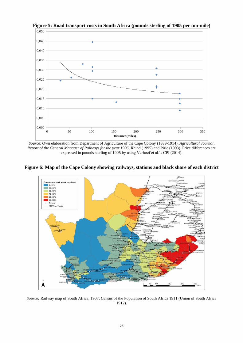
Figure 5: Road transport costs in South Africa (pounds sterling of 1905 per ton-mile)

Source: Own elaboration from Department of Agriculture of the Cape Colony (1889-1914), Agricultural Journal,

Report of the General Manager of Railways for the year 1906, Rhind (1995) and Pirie (1993). Price differences are

expressed in pounds sterling of 1905 by using Verhoef et al.’s CPI (2014).

Figure 6: Map of the Cape Colony showing railways, stations and black share of each district

Source: Railway map of South Africa, 1907; Census of the Population of South Africa 1911 (Union of South Africa

1912).

0,000

0,005

0,010

0,015

0,020

0,025

0,030

0,035

0,040

0,045

0,050

0 50 100 150 200 250 300 350

Distance (miles)

25

Figure 7: Map of eastern parts of the Cape Colony showing railways, stations and black share

of each district

Source: Railway map of South Africa, 1907; Census of the Population of South Africa 1911 (Union of South Africa

1912).

26