Point processes, cost, and the growth of rank in locally compact

groups

Miklos Abert and Sam Mellick∗

February 16, 2021

Abstract

Let G be a locally compact, second countable, unimodular group that is nondiscrete andnoncompact. We explore the theory of invariant point processes on G.

We show that every free probability measure preserving (pmp) action of G can be realizedby an invariant point process.

We analyze the cost of pmp actions of G using this language. We show that amongfree pmp actions, the cost is maximal on the Poisson processes. This follows from showingthat every free point process weakly factors onto any Poisson process and that the cost ismonotone for weak factors, up to some restrictions. We apply this to show that G× Z hasfixed price 1, solving a problem of Carderi.

We also show that when G is a semisimple real Lie group, the rank gradient of anyFarber sequence of lattices in G is dominated by the cost of the Poisson process of G. This,in particular, implies that if the cost of the Poisson process of SL2(C) vanishes, then theratio of the Heegaard genus and the rank of a hyperbolic 3-manifold tends to infinity overFarber chains.

1 Introduction

Let G be a locally compact, second countable, unimodular group that is nondiscrete andnoncompact, endowed with a Haar measure λ. We think of λ as an inherent parameterof G, as all the notions trivally scale with λ. Throughout the paper, we will make theseassumptions on G except when stated otherwise.

A point process Π on G is a random closed and discrete subset Π of G. More precisely,it is a random variable taking values in the configuration space of G:

M = M(G) = ω ⊆ G | ω is closed and discrete.

When the law of Π is invariant under the left G-action, we call Π an invariant point process.When G is discrete, a point process becomes an invariant percolation, a notion with a well-developed theory, see [LP16] and references therein. We do not assume the reader has anyknowledge of point process theory and have made the paper as self-contained as possible.

Invariant point processes are examples of probability measure preserving (pmp) actions.Recall that a pmp action is essentially free (or simply free for short) if the stabiliser ofalmost every point in the action space is trivial. In the particular case of point processes,this means that the set of points will almost surely have no symmetries. Our first theoremshows that actually every free pmp action can be realised this way.

Theorem 1. Every free pmp action of G is isomorphic to a point process on G.

Note that freeness is a necessary condition here as can be seen from the action of R2 onR2/(Z× R). This action is however a point process on a homogeneous space of R2.

The proof of Theorem 1 exhibits an analogy between point processes of locally compactgroups and the symbolic dynamics of countable groups. For a pmp action of a countable

∗This work was partially supported by ERC Consolidator Grant 648017.

1

arX

iv:2

102.

0771

0v1

[m

ath.

GR

] 1

5 Fe

b 20

21

group Γ, every Borel partition of the underlying space gives rise to an invariant randomcoloring of Γ by considering the orbit of a random point of the underlying space. Similarly,every cross section of a free pmp action of G, when considering its intersection with theG-orbit of a random point, will become a point process on G. So point processes serve asstochastic visualizations of pmp actions of locally compact groups, just like invariant randomcolorings do for countable groups. This paper aims to show that this visualization leads tonew and meaningful results.

The correspondence above and the classical theorem of Forrest [For74] on the existenceof cross sections (see also [KPV15] and Section 3.B of [Kec19]) immediately yields that everyfree pmp action factors onto an invariant point process. The factor map can be upgradedto an isomorphism by using a marked point process. These are random discrete subsetswhere each point carries a mark from some mark space (for example, a finite set of colours).Then Theorem 1 is proved by showing that every marked point process is isomorphic to anunmarked one, by “spatially encoding” the marks.

We now introduce the cost of a point process Π on G. A factor graph G of Π is anequivariantly and measurably defined graph G (Π) whose vertex set is Π. For example, onecan define the distance graph for r > 0 to be the set of pairs g, h ∈ Π with d(g, h) < r,where d is a left-invariant metric on G. Informally speaking, the cost of Π is defined as theinfimum of the average degrees over connected factor graphs of Π, suitably normalised tobe an isomorphism invariant. For precise definitions see Section 4.

The cost of pmp actions of countable groups has been an active subject in the last twentyyears, see Gaboriau’s paper [Gab] and the survey paper [Fur09] for the literature. It hasbeen known in the community that cross sections naturally allow one to extend the notionof cost to free pmp actions of locally compact groups, but due to the lack of results, thenotion stayed dormant. The first explicit appearance of the definition can be found in arecent paper of Carderi [Car18]. The definition we work with is essentially equivalent to his,but we develop it intrinsically as a point process theoretic notion.

One of the most important family of processes on a discrete group is Bernoulli perco-lations Ber(p). The natural analogue of this family for non discrete groups is the Poissonpoint process of intensity t > 0. Here the intensity of an invariant point process is theexpected number of points which fall in a set of unit volume. This quantity can be shown tobe independent of the choice of set. An explicit description of Poisson point processes willbe given later, but one should know that these processes are “completely independent”.

Theorem 2. Poisson point processes have maximal cost among all free pmp actions on G.In particular, the cost of a Poisson point process does not depend on its intensity.

We denote the cost of a Poisson point process on G by cP (G). The above result canbe looked at as a locally compact analogue of a result of Abert and Weiss [AW13] wherethey show that for a countable group, Bernoulli actions have maximal cost among all pmpactions.

A central open problem in cost theory is the Fixed Price problem of Gaboriau, that askswhether all free pmp actions of a countable group have the same cost. This is also open inthe locally compact setting.

Question 3. Is it true that all free point processes on G have the same cost?

Gaboriau [Gab02] asks if for a countable pmp equivalence relation, the cost of the relationequals its first L2 Betti number β1(G) plus 1. Note that an affirmative answer for this wouldimply an affirmative answer to Question 1, as well, using the cross section correspondence.

Since the cost of any free process is at least one, a viable way to prove that a group hasfixed price one is by showing that the Poisson point process admits connected factor graphswith average degree 1 + ε for all ε > 0. We succeed in this for the first nontrivial case,answering a question of Carderi [Car18]:

Theorem 4. Every free pmp action of G × Z has cost one if G is compactly generated.More generally, if G is compactly generated and admits a noncompact amenable normalsubgroup, then G has fixed price one.

Our proof is truly a stochastic proof in nature as it essentially uses some special propertiesof Poisson point processes.

2

In countable cost theory, it remains an open question if the direct product Γ × ∆ oftwo infinite countable groups Γ and ∆ has fixed price one. It is known to hold if one ofthe groups contains a fixed price one subgroup. When trying to generalize Theorem 4 toarbitrary products, we seem to hit a somewhat similar barrier.

Question 5. Let G and H be compactly generated but noncompact groups. Does G ×Hhave fixed price one?

Another application of Theorem 2 concerns the growth of the minimal number of gen-erators (the rank gradient) for a sequence of lattices in semisimple real Lie groups. Recallthat a discrete subgroup Γ ≤ G is a lattice if it has finite covolume in G. Let d(Γ) denotethe minimal number of generators (also known as the rank) of Γ. When G is a semisimpleLie group, d(Γ) is finite and by a theorem of Gelander [Gel11], we have

d(Γ)− 1

vol(G/Γ)≤ C

for some constant C only depending on G.A sequence of lattices Γn in G is Farber, if G/Γn approximates G in the Benjamini-

Schramm topology, or, equivalently, if the corresponding invariant random subgroups weaklyconverge to the trivial subgroup. The sequence is uniformly discrete if there exists C > 0such that the infimal injectivity radius is bounded below by C for G/Γn.

Theorem 6. Let G be a semisimple real Lie group and let Γn be a Farber sequence oftorsion free lattices in G. Then

lim supn→∞

d(Γ)− 1

vol(G/Γ)≤ cP(G)− 1.

In particular, if the Poisson point process has cost 1 then the rank grows sublinearly inthe covolume, for Farber sequences of torsion free lattices. This correspondance connectscomputing the cost of the Poisson process to some exciting open problems that have beeninvestigated extensively. Theorem 6 extends Carderi’s result [Car18] who proved it foruniformly discrete (in particular, cocompact) Farber sequences. For semisimple Lie groups,we expect the cost of Poisson to follow a rather simple rule.

Question 7. Let G be a semisimple real Lie group that is not a compact extension ofSL2(R). Is cP(G) = 1?

Note that by a forthcoming work of Gaboriau et al. SL2(R) is treeable and has fixedprice > 1.

We now showcase three concrete cases for a semisimple Lie group where computing thecost of the Poisson would solve known problems of a different nature.

Case G = SL2(C). If cP(G) > 1, then we get free point processes in G with differentcost. Moreover, we also get a countable equivalence relation whose first L2 Betti number isnot equal to its cost-1, answering a question of Gaboriau [Gab02]. If, on the other hand,cP(G) = 1, then we get that the Heegaard genus divided by the rank of the fundamentalgroup of a (compact) hyperbolic 3-manifold can get arbitrarily large. In fact, we yieldthis for any expander Farber sequence of hyperbolic 3-manifolds, which is understood asthe typical behavior. Note that it is a longstanding open problem whether this ratio isabsolutely bounded over all 3-manifolds, and in fact it was only proved recently in the deeppaper of Li [Li13] that for compact hyperbolic 3-manifolds, the Heegaard genus can differfrom the rank.

Case when G has higher rank. For these Lie groups, Fraczyk recently proved in abeautiful paper [Fra18] that the growth of the first mod 2 homology vanishes for Farbersequences in G. Surprisingly, his method does not seem to carry over to odd primes, so forprimes other than 2, this is still an open problem. As the rank is an upper bound for thefirst mod p homology of a discrete group, proving cP(G) = 1 would settle this problem.

By a standard induction argument, proving cP(G) = 1 would show that any lattice in Ghas fixed price 1, a problem of Gaboriau that is still open for cocompact lattices.

Case when G has higher rank and property (T). Using [ABB+17], for semisimpleLie groups with (T) one can actually omit the Farber condition.

3

Corollary 8. Let G be a higher rank semisimple real Lie group with property (T) and letΓn be any sequence of torsion free lattices in G with vol(G/Γn)→∞. Then

lim supn→∞

d(Γn)− 1

vol(G/Γn)≤ cP(G)− 1.

In particular, if cP(G) = 1, then we get a totally uniform vanishing theorem for thegrowth of rank for lattices in these groups, including SL(d,R) (d ≥ 3). It is shown in[AGN+17] that any Farber sequence in SL(3,Z) has vanishing rank gradient, but the uniformversion is wide open.

Note that in their very recent paper Lubotzky and Slutsky [LS21] showed that in theabove situation, every sequence of non-uniform lattices will have rank gradient 0. Theirproof uses deep classical results on non-uniform lattices, like arithmeticity and the Congru-ence Subgroup Property but in turn gives a much stronger upper bound for the number ofgenerators than what we ask, logarithmic in the covolume. In most cases, they can evenimprove this with a loglog factor. Their methods do not seem to readily generalize to co-compact lattices. Our purely geometric approach may have the potential to be applied morewidely but the payoff is that, being a limiting argument, it is not expected to yield suchexplicit estimates.

The proof of Theorem 2 uses the stochastic visualisation method to show that everyfree action is “sufficiently rich” in randomness to “simulate” the Poisson point process. Inparticular, connected factor graphs of the Poisson point process can be transferred to anarbitrary free process in a way that can at worst decrease the average degree. Simulationhere refers to weak factoring, a notion we introduce that is inspired by weak containment ofactions, see the survey of Kechris and Burton [Kec19].

For invariant point processes Π and Υ, we say that Υ is a factor of Π if there exists aG-equivariant Borel map Φ : M→ M such that Φ(Π) = Υ. We say that Υ is a weak factorof Π if there exist factor maps Φ1,Φ2, . . . of Π such that Φn(Π) converges weakly to Υ.

Theorem 9. Let Π be a free point process on G. Then Π weakly factors onto the Poissonpoint process of intensity t, for all t.

In particular, Poisson processes on G of different intensities weakly factor onto eachother. More is known in the amenable case: Ornstein and Weiss showed [OW87] that for alarge class of amenable groups, the Poisson point processes of different intensity are in factisomorphic as actions (see [SW+19] for an alternative construction on Rn with additionalproperties).

The proof of Theorem 9 revolves around IID-marked processes. Let [0, 1]Π denote therandom [0, 1]-marked subset of G whose underlying set is Π and has independent and identi-cally distributed Unif[0, 1] random variables. We call this the IID of Π. Once this definitionand that of the Poisson point process is understood, one can readily see that the IID of anyprocess factors onto the Poisson point process. We then prove:

Theorem 10. Let Π be a free point process on G. Then Π weakly factors onto [0, 1]Π, itsown IID.

Surprisingly, it is not entirely trivial to show that weak factoring is a transitive notion.In particular, Theorem 10 implies that free point processes weakly factor onto the Poissonpoint process.

We next investigate how cost behaves with respect to factor maps. It is easy to seethat it can only increase under a factor map: if Π factors onto Υ, then cost(Π) ≤ Υ. Inparticular, this shows that cost is an isomorphism invariant of actions. This monotonicityof cost under factor maps can be pushed further:

Theorem 11. Suppose Π weakly factors onto Υ, as witnessed by a sequence of factor mapsΦn(Π) weakly converging to Υ. Under appropriate tightness conditions on Π,Υ, and thesequence Φn, we have cost(Π) ≤ cost(Υ).

See Section 5.2 for a precise statement. This cost monotonicity theorem, limited as it is,is powerful enough to prove that the Poisson point process has maximal cost amongst allfree processes.

The paper is structured as follows:

4

In Section 1, we give the basic definitions and notations of point processes for those whohave never encountered them before, and describe the most important examples of pointprocesses for our work.

In Section 2, we introduce the Palm measure of a point process and the rerootinggroupoid.

In Section 3, we define the cost of an invariant point process and prove basic propertiesof it.

In Section 4, we define weak factoring of point processes and prove that (in certaincircumstances) cost is monotone with respect to weak factoring. We use this to show thatthe Poisson has maximal cost amongst all free processes.

In Section 5, we use the fact that the Poisson has maximal cost to give the first nontrivialexamples of nondiscrete groups with fixed price.

In Section 6, we connect the rank gradient of sequences of lattices in a group with thecost of the Poisson point process on said group.

In the appendix, we include a summary of necessary technical facts from point processtheory with references for proofs, a discussion of how our theory extends to point processeson homogeneous spaces, and how it connects with cross-sections.

2 Point processes and factors of interest

Let (Z, d) denote a complete and separable metric space (a csms). A point process on Z isa random discrete subset of Z. We will also study random discrete subsets of Z that aremarked by elements of an additional csms Ξ. Typically Ξ will be a finite set that we thinkof as colours.

Definition 12. The configuration space of Z is

M(Z) = ω ⊂ Z | ω is discrete,

and the Ξ-marked configuration space of Z is

ΞM(Z) = ω ⊂ Z × Ξ | ω is discrete, and if (g, ξ) ∈ ω and (g, ξ′) ∈ ω then ξ = ξ′.

Note that ΞM(Z) ⊂ M(Z × Ξ). We think of a Ξ-marked configuration ω ∈ ΞM(Z) as adiscrete subset of Z with labels on each of the points (whereas a typical element of M(Z×Ξ)is a discrete subset where each point has possibly multiple marks).

If ω ∈ ΞM(Z) is a marked configuration, then we will write ωz for the unique element ofΞ such that (z, ωz) ∈ ω.

The Borel structure on configuration spaces is exactly such that the following pointcounting functions are measurable. Let U ⊆ Z be a Borel set. It induces a functionNU : M(Z)→ N0 ∪ ∞ given by

NU (ω) = |ω ∩ U |.

We will primarily be interested in point processes defined on locally compact and secondcountable (lcsc) groups G. Such groups admit a unique (up to scaling) Haar measure λ, wefix such a choice. Recall:

Theorem 13 (Struble’s theorem, see Theorem 2.B.4 of [CdlH16]). Let G be a locallycompact topological group. Then G is second countable if and only if it admits a proper1

left-invariant metric.

Such a metric is unique up to coarse equivalence (bilipschitz if the group is compactlygenerated). We fix d to be any such metric.

We mostly consider the configuration space of a fixed group G. So out of notationalconvenience let us write M = M(G) and ΞM = ΞM(G). The latter here is an abuse ofnotation: formally ΞM ought to denote the set of functions from M to Ξ, but instead we areusing it to denote the set of functions from elements of M to Ξ.

1Recall that a metric is proper if closed balls are compact.

5

Note that the marked and unmarked configuration spaces of G are Borel G-spaces. Tospell this out, Gy M by g · ω = gω and Gy ΞM by

g · ω = (gx, ξ) ∈ G× Ξ | (g, ξ) ∈ ω.

Definition 14. A point process on G is a M(G)-valued random variable Π : (Ω,P)→M(G).Its law or distribution µΠ is the pushforward measure Π∗(P) on M(G). It is invariant if itslaw is an invariant probability measure for the action Gy M(G).

The associated point process action of an invariant point process Π is Gy (M(G), µΠ).

Some remarks and caveats are in order:

• Point processes which are not invariant are very much of interest, but will only playa particular role in this work. Thus we will sometimes say “point process” when wemean invariant point process.

• Speaking properly, we are discussing simple point processes, that is, those where eachpoint has multiplicity one. We will discuss this more later.

• Ξ-marked point processes are defined similarly, with ΞM taking the place of M. Thereisn’t much difference between marked point processes and unmarked ones for our pur-poses (it’s just a case of which is more convenient for the particular problem at hand).Thus “point process” might also mean “marked point process”.

• One could certainly define point processes on a discrete group, but this is better knownas percolation theory. We are trying to move beyond that, so we will almost alwaysimplicitly assume G is nondiscrete.

• The other case of interest we will discuss is Isom(S)-invariant point processes on S,where S is a Riemannian symmetric space. For instance, one would consider isometryinvariant point processes on Euclidean space Rn or hyperbolic space Hn. We willdiscuss this case more in the appendix.

• Our interest in point processes is almost exclusively as actions. We will therefore rarelydistinguish between a point process proper and its distribution. Thus we may useexpressions like “suppose µ is a point process” to mean “suppose µ is the distributionof some point process”.

• The configuration space of any Polish space will be Polish, so the probability theory ofpoint processes on such spaces is well behaved. The metric properties of configurationspaces that we require are listed in the appendix, with references for proofs.

Definition 15. The intensity of a point process µ is

int(µ) =1

λ(U)Eµ [NU ] ,

where U ⊂ G is any Borel set of positive (but finite) Haar measure, and NU (ω) = |ω ∩ U |is its point counting function.

To see that the intensity is well-defined (that is, does not depend on our choice ofU), observe that the function U 7→ Eµ[NU ] defines a Borel measure on G which inheritsinvariance from the shift invarance of µ. So by uniqueness of Haar measure, it is somescaling of our fixed Haar meausure λ – the intensity is exactly this multiplier. We also seethat whilst the intensity depends on our choie of Haar measure, it scales linearly with it.

Note that a point process has intensity zero if and only if it is empty almost surely.

2.1 Examples of point processes

Example (Lattice shifts). Let Γ < G be a lattice, that is, a discrete subgroup that admits aninvariant probability measure ν for the action Gy G/Γ. The natural map M(G/Γ)→M(G)given by

ω 7→⋃aΓ∈ω

aΓ

is left-equivariant, and hence maps invariant point processes on G/Γ to invariant pointprocesses on G. In particular, we have the lattice shift, given by choosing a ν-random pointaΓ.

6

Example (Induction from a lattice). Now suppose one also has a pmp action Γ y (X,µ).It is possible to induce this to a pmp action of G on G/Γ×X. This can be described as anX-marked point process on G. To do this, fix a fundamental domain F ⊂ G for Γ. Choosef ∈ F uniformly at random, and independently choose a µ-random point x ∈ X. Let

Π = (fγ, γ · x) ∈ G×X | γ ∈ Γ.

Then Π is a G-invariant X-marked point process.

In this way one can view point processes as generalised lattice shift actions. Note thatthere are groups without lattices (for instance Neretin’s group, see [BCGM12]), but everygroup admits interesting point processes, as we discuss now. The most fundamental ofthese is known as the Poisson point process. We will define this after reviewing the Poissondistribution:

Recall that a random integer N is Poisson distributed with parameter t > 0 if

P[N = k] = exp(−t) tk

k!.

We write N ∼ Pois(t) to denote this. It is convenient to extend this definition to t = 0and t = ∞ by declaring N ∼ Pois(0) when N = 0 almost surely and N ∼ Pois(∞) whenN =∞ almost surely.

Definition 16. Let X be a complete and separable metric space equipped with a non-atomicBorel measure λ.

A point process Π on X is Poisson with intensity t > 0 if it satisfies the following twoproperties:

(Poisson point counts) for all U ⊆ G Borel, NU (Π) is a Poisson distributed randomvariable with parameter tλ(U), and

(Total independence) for all U, V ⊆ G disjoint Borel sets, the random variables NU (Π)and NV (Π) are independent.

For reasons that should not be immediately apparent, both of the above defining prop-erties are equivalent. We will write Pt for the distribution of such a random variable, orsimply P if the intensity is understood.

We think of the Poisson point process as a completely random scattering of points in thegroup. It is an analogue of Bernoulli site percolation for a continuous space.

We now construct the process (somewhat) explicitly. Partition G into disjoint Borel setsU1, U2, . . . of positive but finite volume. For each of these, independently sample from a Pois-son distribution with parameter tλ(Ui). Place that number of points in the correspondingUi (independently and uniformly at random).

This description can be turned into an explicit sampling rule2, if one desires.For proofs of basic properties of the Poisson point process (such as the fact that it

does not depend on the partition chosen above), see the first five chapters of Kingman’sbook [Kin93].

Definition 17. A pmp action G y (X,µ) is ergodic if for every G-invariant measurablesubset A ⊆ X, we have µ(A) = 0 or µ(A) = 1.

The action is mixing if for all measurable A,B ⊆ (X,µ) we have

limg→∞

µ(gA ∩B) = µ(A)µ(B).

The action is essentially free if stabG(x) = 1 for µ almost every x ∈ X. In the case ofpoint process actions we will sometimes use the term aperiodic to refer to this.

Proposition 18. The Poisson point process actions Gy (M,Pt) on a noncompact groupG are essentially free and ergodic (in fact, mixing).

2That is, one can define a measurable function f :∏

nXn → M defined on an appropriate product ofprobability spaces such that the pushforward measure is the distribution of the Poisson point process.

7

A proof of freeness that is readily adaptable to our setting can be found as Proposition2.7 of [ABB+17]. For ergodicity and mixing, see the proof of the discrete case in Proposition7.3 of the Lyons-Peres book [LP16]. It directly adapts, once one knows the required cylindersets exist.

Although the subscript t suggests that the Poisson point processes form a continuumfamily of actions, this is not always the case:

Theorem 19 (Ornstein-Weiss). Let G be an amenable group which is not a countableunion of compact subgroups. Then the Poisson point process actions G y (M,Pt) are allisomorphic.

The following definition uses notation that does not appear in the literature (the objectof course does, but there does not appear to be a symbolic representation for it):

Definition 20. If Π is a point process, then its IID version is the [0, 1]-marked point process[0, 1]Π with the property that conditional on its set of points, its labels are independent andIID Unif[0, 1] distributed. If µ is the law of Π, then we will write [0, 1]µ for the law of [0, 1]Π.

One can define the IID of a point process over spaces other than [0, 1] (for instance,[n] = 1, 2, . . . , n with the counting measure), but we will only use the full IID.

Remark 21. As we’ve mentioned, [0, 1]-marked point processes on G are particular exam-ples of point processes on G × [0, 1]. One can show (see Theorem 5.6 of [LP18]) that thePoisson point process on G× [0, 1] with respect to the product measure λ⊗ Leb is just theIID version of the Poisson point process on G, a fact which we will make use of later.

Proposition 22. The IID Poisson point process on a noncompact group is ergodic (and infact mixing).

This can be seen by viewing the IID Poisson on G as the Poisson point process on G×S1,restricted to G. Note that the restriction of a mixing action to a noncompact subgroup ismixing.

Remark 23. One can define “the IID” of any probability measure preserving countableBorel equivalence relation, see [BHI18]. This construction is known as the Bernoulli exten-sion, and is ergodic if the base space is ergodic.

Proposition 24. Let Π be a point process on a group G which is non-empty almost surely.Then |Π| =∞ almost surely if and only if G is noncompact.

Proof. It is immediate that any point process on a compact group must be finite almostsurely (as it is a discrete subset of the space).

Now suppose Π is a non-empty point process on G which is finite almost surely. Then theIID of this process [0, 1]Π still has this property. We define the following G-valued randomvariable:

f([0, 1]Π) = the unique x ∈ Π with maximal label in [0, 1]Π.

The invariance of the point process translates into equivariance of the map f : [0, 1]M → G.Thus this random variable’s law is an invariant probability measure on G. Such a measureexists exactly when G is compact.

2.2 Factors of point processes

Definition 25. A point process factor map is a G-equivariant and measurable map Φ :M → M. If µ is a point process and Φ is only defined µ almost everywhere, then we willcall it a µ factor map.

We will be interested in two monotonicity conditions:

• if Φ(ω) ⊆ ω for all ω ∈M, we will call Φ a thinning (and usually denote it by θ), and

• if Φ(ω) ⊇ ω for all ω ∈M, we will call Φ a thickening (and usually denote it by Θ).

We use the same terms for marked point processes as well.

8

Remark 26. There are two possible ways to interpret the above monotonicity conditionsfor a Ξ-marked point process, depending on what you want to do with the mark space. Onecan consider

Φ : ΞM → ΞM, or Φ : ΞM →M.

In the former case, the definition above works verbatim. In the latter case, one shouldinterpret a statement like “ω ⊆ Φ(ω)” as “ω is contained in the underlying set π(Φ(ω)) ofΦ(ω), where π : ΞM →M is the map that forgets labels.

The following example is implicit in the literature, but is not usually named and doesnot have a consistent symbolic representation. We will use it enough that we must name it:

Example (Metric thinning). Let δ > 0 be a tolerance parameter. The δ-thinning is theequivariant map θδ : M→M given by

θδ(ω) = g ∈ ω | d(g, ω \ g > δ.

When θδ is applied to a point process, the result is always a δ-separated point process(but possibly empty).

We define θδ in the same way for marked point processes (that is, it simply ignores themarks).

Example (Independent thinning). Let Π be a point process. The independent p-thinningdefined on its IID [0, 1]Π is given by

Ip([0, 1]Π) = g ∈ Π | Πg ≤ p.

One can show that independent p-thinning of the Poisson point process of intensity t > 0yields the Poisson point process of intensity pt, as one would expect. See Chapter 5 of [LP18]for further details.

Example (Constant thickening). Let F ⊂ G be a finite set containing the identity 0 ∈ G,and Π be a point process which is F -separated in the sense that Π ∩ Πf = ∅ for allf ∈ F \ 0. Then there is the associated thickening ΘF (Π) = ΠF . It is intuitively obviousthat int(ΘF (Π)) = |F | int(Π). This can be formally established as follows: let U ⊆ G be ofunit volume. Then

int(ΘF (Π)) = E|U ∩ΠF | By definition

=∑f∈F

E|U ∩Πf | By F -separation

=∑f∈F

E∣∣Uf−1 ∩Π

∣∣=∑f∈F

E|U ∩Π| By unimodularity

= |F | int(Π).

This is the first real appearance of our unimodularity assumption.In particular, we can demonstrate that int ΘF (Π) = |F | int Π is not automatically true

without unimodularity. For this, let Π denote the unit intensity Poisson point process on G,and F = 0, f where f ∈ G is chosen such that λ(Uf−1) < 1. Then

∣∣Uf−1 ∩Π∣∣ is Poisson

distributed with parameter λ(Uf−1), and so by the above calculation int ΘF (Π) < 2 · int Π.

Monotone maps have been investigated in the specific case of the Poisson point processon Rn. We note the following interesting theorems:

Theorem 27 (Holroyd, Peres, Soo [HLS11]). Let s > t > 0. Then the Poisson point processon Rn of intensity s can be thinned to the Poisson point process of intensity t. That is,there exists an equivariant and deterministic map θ : (M(R),Ps)→ (M(R),Pt).

Theorem 28 (Gurel-Gurevich and Peled [GGP13]). Let s > t > 0 be intensities. Then thePoisson point process on Rn of intensity s cannot be thickened to the Poisson point processof intensity t. That is, there is no equivariant and deterministic map Θ : (M(R),Ps) →(M(R),Pt).

9

We stress in the above theorems the deterministic nature of the maps. If one is allowedadditional randomness (that is, one asks for a factor of IID map), then both theorems areeasily established.

We note the following fact, which we will use (and prove) later after developing somenotation.

Example. If Π is any point process, then its IID factors onto the Poisson (in fact, onto theIID Poisson).

Definition 29. A factor Ξ-marking of a point process is a G-equivariant map C : M→ ΞM

such that the underlying subset in G of C (ω) is ω. That is, C is a rule that assigns a markfrom Ξ to each point of ω in some deterministic way. Again, if C is only defined µ almosteverywhere then we will call it a µ factor Ξ-marking.

Example. Let θ : M → M be a thinning. Then the associated 2-colouring is Cθ : M →0, 1M given by

Cθ(ω) = (g,1[g ∈ θ(ω)]) ∈ G× 0, 1 | g ∈ ω.

We will see that all markings are built out of thinnings in a similar way.

Remark 30. There is a difference between the thinning map θ and the resulting thinnedprocess θ∗(µ) that can be a source for confusion. Passing to the thinned process (in principle)can lose information about µ.

For example, let Π denote a Poisson point process on G and Υ an independent randomshift of a lattice Γ < G. Define the following thinning θ : M→M by

θ(ω) = g ∈ ω | gΓ ⊆ ω.

Then θ(Π ∪Υ) = Υ, and so the thinning completely loses the Poisson point process.

Definition 31. Let Φ : M→ M be a factor map. We think of its input ω as being red, itsoutput Φ(ω) as being blue, and their overlap ω ∩ Φ(ω) as being purple.

For g ∈ ω, let Colour(g) ∈ Red, Blue, Purple be

Colour(g) =

Red If g ∈ ω \ Φ(ω),

Blue If g ∈ Φ(ω) \ ω,Purple If g ∈ ω ∩ Φ(ω).

Now define ΘΦ : M→ Red, Blue, PurpleM to be the following input/output thickening ofΦ (see also Figure 31):

ΘΦ(ω) = (g, Colour(g)) ∈ G× Red, Blue, Purple | g ∈ ω.

Let π : Red, Blue, PurpleM → M be the projection map that deletes red points andthen forgets colours, that is,

π(ω) = g ∈ ω | ωg ∈ Blue, Purple.

Remark 32. Observe that Φ = π ΘΦ – that is, an arbitrary factor map decomposes asthe composition of a thinning and a thickening. In this way we can often reduce the studyof arbitrary factors to that of monotone factors.

Definition 33. The space of graphs in G is

Graph(G) = (V,E) ∈M(G)×M(G×G) | E ⊆ V × V .

This is a Borel G-space (with the diagonal action).A factor graph is a measurable and G-equivariant map Φ : M(G)→ Graph(G) with the

property that the vertex set of Φ(ω) is ω.If a factor graph is connected, then we will refer to it as a graphing.

Remark 34. The elements of Graph(G) are technically directed graphs, possibly withloops, and without multiple edges between the same pair of vertices. It’s possible to define(in a Borel way) whatever space of graphs one desires (coloured, undirected, etc.) by takingappropriate subsets of products of configuration spaces.

10

Figure 1: This is how you should picture the input/output thickening of a factor map.

Remark 35. One might prefer to call factor graphs as above monotone factor graphs. Ourterminology follows that of probabilists, see for instance [HP05]. We have not found a usefor the less restrictive factor graph concept.

Example. The distance-R factor graph is the map DR : M→ Graph(G) given by

DR(ω) = (g, h) ∈ ω × ω | d(g, h) ≤ R.

The connectivity properties of this graph fall under the purview of continuum percolationtheory, see for instance [MR96].

3 The rerooting equivalence relation and groupoid

We now introduce a pair of algebraic objects that capture factors of a point process. Forexposition’s sake, we will first discuss unmarked point processes on a group G.

Definition 36. The space of rooted configurations on G is

M0(G) = ω ∈M(G) | 0 ∈ ω.

If G is understood, then we will drop it from the notation for clarity.The rerooting equivalence relation on M0 is the orbit equivalence relation of G y M

restricted to M0. Explicitly:

R = (ω, g−1ω) ∈M0 ×M0 | g ∈ ω.

This defines a countable Borel equivalence relation structure on M0. It is degeneratewhenever ω ∈M0 exhibits symmetries: for instance, the equivalence class of Z viewed as anelement of M0(R) is a singleton. We are usually interested in essentially free actions, wheresuch difficulties will not occur. Nevertheless, we do care about lattice shift point processesand so we will introduce a groupoid structure that keeps track of symmetries.

The space of birooted configurations is

−→M0 = (ω, g) ∈M0 ×G | g ∈ ω.

We visualise an element (ω, g) ∈−→M0 as the rooted configuration ω ∈ M0 with an arrow

pointing to g ∈ ω from the root (ie, the identity element of G).

11

The above spaces form a groupoid (M0,−→M0) which we will refer to as the rerooting

groupoid. Its unit space is M0 and its arrow space is−→M0. We can identify M0 with M0×0 ⊂−→

M0.The multiplication structure is as follows: we declare a pair of birooted configurations

(ω, g), (ω′, h) in−→M0 to be composable if ω′ = g−1ω, in which case

(ω, g) · (ω′, h) := (ω, gh).

Note that if Γ < G is a discrete subgroup (so Γ ∈M0(G)), then the above multiplicationis just the usual one.

The source map s :−→M0 →M0 and target map t :

−→M0 →M0 are

s(ω, g) = ω, and t(ω, g) = g−1ω.

Note that the rerooting groupoid is discrete in the sense that s−1(ω) is at most countablefor all ω ∈M0.

Remark 37. Let Maper0 denote the set of rooted configurations ω that are aperiodic in the

sense that stabG(ω) = e. Then the groupoid generated by Maper0 in M0 is principal3.

Definition 38. If Ξ is a space of marks, then the space of Ξ-marked rooted configurationsis

ΞM0 = ω ∈ ΞM | ∃ξ ∈ Ξ such that (0, ξ) ∈ ω.

The Ξ-marked rerooting groupoid is defined as previously, with ΞM0 taking the place ofM0.

3.1 Borel correspondences between the groupoid and factors

Suppose θ : M → M is an equivariant and measurable thinning. Then we can associate toit a subset of the rerooting groupoid, namely

Aθ = ω ∈M | 0 ∈ θ(ω).

This association has an inverse: given a Borel subset A ⊆ M0, we can define a thinningθA : M→M

θA(ω) = g ∈ ω | g−1ω ∈ A.

Thus we see that Borel subsets A ⊆ M0 of the rerooting groupoid correspond to Borelthinning maps θ : M→M.

In the Ξ-marked case, one associates to a subset A ⊆ ΞM0 a thinning θA : ΞM → ΞM.In a similar way, we can see that if P : M0 → [d] is a Borel partition of M0 into d classes,

then there is an associated factor [d]-colouring C P : M→ [d]M given by

C P (ω) = (g, P (g−1ω) ∈ G× [d] | g ∈ ω,

and given a factor [d]-colouring C : M → [d]M one associates the partition PC : M0 → [d]given by

P (ω) = c, where c is the unique element of [d] such that (0, c) ∈ C (ω).

Again, these associations are mutual inverses.More generally, we see that Borel factor Ξ-markings C : M → ΞM correspond to Borel

maps P : M0 → Ξ.Now suppose that G : M → Graph(G) is an equivariant and measurable factor graph.

Then we can associate to it a subset of the rerooting groupoid’s arrow space, namely

AG = (ω, g) ∈−→M0 | (0, g) ∈ G (ω).

3Recall that a groupoid is principal if its isotropy subgroups are all trivial. That is, the groupoid structure isjust that of an equivalence relation

12

In the other direction, we associate to a subset A ⊆−→M0 the factor graph G A : M →

Graph(G)G A (ω) = (g, h) ∈ ω × ω | (g−1ω, g−1h) ∈ A .

Thus we see that Borel subsets A ⊆−→M0 of the rerooting groupoid’s arrow space corre-

spond to Borel factor (directed) graphs G : M→ Graph(G).

Remark 39. If µ is a point process, then the correspondence still works in one direction:

namely, we can associate subsets A ⊂M0 (or A ⊆−→M0) to µ-thinnings θA : (M, µ)→M (or

µ-factor graphs GA : (M, µ)→M respectively).We run into trouble in the other direction: suppose θ : M → M is a thinning, but only

defined µ almost everywhere. We wish to restrict it to M0, but a priori this makes no sense– that is a subset of measure zero. It turns out that there is a way to make sense of this dueto equivariance, but it will require some more theory that we explain in the next section.

3.2 The Palm measure

We will now associate to a (finite intensity) point process µ a probability measure µ0 definedon the rerooting groupoid M0. When the ambient space is unimodular, this will turn thererooting groupoid into a probability measure preserving (pmp) discrete groupoid.

Informally, the Palm measure of a point process Π is the process conditioned to containthe root. A priori this makes no sense (the subset M0 has probability zero), but there isan obvious way one could interpret the statement: condition on the process to contain apoint in an ε ball about the root, and take the limit as ε goes to zero. See Theorem 13.3.IVof [DVJ07] and Section 9.3 of [LP18] for further details.

We will instead take the following concept of relative rates as our basic definition:

Definition 40. Let Π be a point process of finite intensity with law µ. Its (normalised)Palm measure is the probability measure µ0 defined on Borel subsets of M0 by

µ0(A) :=int(θA(Π))

int(Π),

where θA is the thinning associated to A ⊆M0.More explicitly,

µ0(A) :=1

int(µ)Eµ[#g ∈ U | g−1ω ∈ A

],

where U ⊆ G is of unit volume.We also define the Palm measure of a Ξ-marked point process similarly, with ΞM0 taking

the place of M0.A Palm version of Π is any random variable Π0 with law µ0. That is, if for all Borel

B ⊆M0 we haveP[Π0 ∈ B] = µ0(B).

We now describe some Palm calculus. If Π is a point process with Palm version Π0 andΦ(Π) is some factor map then we wish to express the Palm version Φ(Π)0 of Φ(Π) in terms ofΠ0 and Φ. The Palm calculus tells us how this is done. It will be sufficient for our purposesto compute the Palm measure of factors for factor which are forgettings, thinnings, colouredthickenings, and colourings. In each case the answer is more or less obvious, so we will givean informal description of the answer and then verify that it satisfies the required property.

Example (Forgetting labels). If Π is a labelled point process, then the Palm measure of Πafter we forget the labels is the same thing as forgetting the labels from the Palm measureΠ0.

We prove this after the following clarification:When talking about the Palm measure for a Ξ-marked point process, it is important in

the above to choose the correct thinning. Recall from Remark 26 that for a subset A ⊆ ΞM0

one can discuss two possible kinds of thinnings, namely

θA : ΞM → ΞM or π θA : ΞM →M,

13

where π : ΞM →M is the map that forgets labels.It is the former kind of thinning one should take.Note that if Π is a Ξ-marked point process, then its intensity remains the same if you

forget the marks, that is, int Π = intπ(Π). More generally, the operation of taking the Palmversion commutes with forgetting labels. That is, π(Π0) = (π(Π))0. To see this, let B ⊆M0,and observe

P[π(Π0) ∈ B] = P[Π0 ∈ π−1(B)]

=int θπ

−1(B)(Π)

int Π

=intπ(θπ

−1(B)(Π))

intπ(Π)

=int θB(π(Π))

intπ(Π)

= P[π(Π)0 ∈ B],

where we simply followed our nose.

Example (Lattice actions). If Γ < G is a lattice, then the Palm measure of the associatedlattice shift is just δΓ – that is, the atomic measure on Γ ∈ M0(G). More generally, ifΓ y (X,µ) is a pmp action, then the Palm measure of the associated induced X-markedpoint process is its symbolic dynamics. That is, the map Σ : (X,µ)→ XM given by

Σ(x) = (γ, γ−1 · x) ∈ G×X | γ ∈ Γ.

pushes forward µ to the Palm measure. In words, you sample a µ-random point x ∈ X andtrack its orbit under Γ (the inverse is an artefact of our left bias).

Remark 41. Suppose Π is a finite intensity point process such that its Palm version is anatomic measure, say Π0 = Ω almost surely where Ω ∈ M0. Then Ω is a lattice in G. Notethat Ω is automatically a discrete subset of G, and a simple mass transport argument showsthat it is a subgroup. The covolume of this subgroup is the reciprocal of the intensity of Π.

Example (Mecke-Slivnyak Theorem). If Π is a Poisson point process, then its Palm measurehas the same law as Π ∪ 0, where 0 ∈ G is the identity.

In fact, this is a characterisation of the Poisson point process: if the Palm measure of µ isobtained by simply adding the root4, then µ is the Poisson point process (of some intensity).

The proof of the above fact can be found in Section 9.2 of [LP18]. As a consequence, thePalm measure of the IID Poisson is the IID of the Palm measure of the Poisson itself.

Example. The Palm version CA(Π)0 of a 2-colouring C : M → 0, 1M determined by asubset A ⊆M0 (as in

Example (Thinnings). The Palm version θ(Π)0 of a thinning θ = θA of Π (determined bya subset A ⊆ M0) is described in terms of its Palm version Π0 as a conditional probabilityas follows:

P[θ(Π)0 ∈ B] = P[θ(Π0) ∈ B | Π0 ∈ A]

for any B ⊆M0.That is, the Palm measure θ(Π)0 can be obtained by sampling from Π0 conditioned that

the root is retained in the thinning, and then applying the thinning.To see this, first one should work from the definitions to show that θB(θA(Π)) =

4More formally, consider the map F : M→ M0 given by F (ω) = ω ∪ 0, by “adding the root” we mean thePalm measure µ0 is the pushforward F∗µ.

14

θA∩(θA)−1(B). Therefore

P[(θ(Π))0 ∈ B] =int θB(θA(Π))

int θA(Π)

=int θA∩(θA)−1(B)(Π)

int Π

/int θA(Π)

int ΠBy the observation

=P[Π0 ∈ A ∩ (θA)−1(B)]

P[Π0 ∈ A]

=P[θ(Π0) ∈ B ∩ Π0 ∈ A]

P[Π0 ∈ A]

=P[θ(Π0) ∈ B ∩ Π0 ∈ A]

P[Π0 ∈ A],

which is exactly the definition of the desired conditional probability.

Example. Let Θ = ΘF be a constant thickening determined by F ⊂ G, as described inExample 2.2. If Π is an F -separated process, then the Palm version Θ(Π)0 of the thickeningΘ(Π) is as follows: sample from Π0, and independently choose to root Θ(Π0) at a uniformly

chosen element X of F . That is, Θ(Π)0d= X−1Θ(Π0).

To see this, we compute5 as follows:

P[Θ(Π)0 ∈ B] =1

int Θ(Π)E[#g ∈ U ∩ΠF | g−1Θ(Π) ∈ B] By definition

=1

|F |1

intµ

∑f∈F

E[#g ∈ U ∩Πf | g−1Θ(Π) ∈ B] By Example 2.2

=1

|F |1

intµ

∑f∈F

E[#g ∈ Uf−1 ∩Π | g−1Π ∈ Θ−1(B)] By equivariance

=1

|F |1

intµ

∑f∈F

E[#g ∈ U ∩Π | g−1Π ∈ Θ−1(B)] By unimodularity

=1

|F |∑f∈F

P[Π0 ∈ Θ−1(B)] By definition

=1

|F |∑f∈F

P[Θ(Π0) ∈ B]

= P[X−1Θ(Π0) ∈ B].

The Palm measure has an associated integral equation. One writes

(λ⊗ µ0)(U ×A) =

∫G

E01[U ×A]dλ(x)

and then invokes the usual machine to extend a statement about measurable sets to oneabout measurable functions. We will refer to the resulting formula as “the CLMM”, anduse it to prove the Mass Transport Principle:

Theorem 42 (Campbell-Little-Mecke-Matthes). Let µ be a finite intensity point processon G with Palm measure µ0. Write E and E0 for the associated integral operators.

If f : G ×M0 → R≥0 is a measurable function (not necessarily invariant in any way),then

E

[∑x∈ω

f(x, x−1ω)

]= int(µ)E0

[∫G

f(x, ω)dλ(x)

].

5When we define the Palm measure of a set B ⊆ M0, we usually write “g ∈ U” rather than “g ∈ U ∩ Π”,as the latter condition g−1Π ∈ B already implies g ∈ Π. For this computation it is better to really spell it outthough.

15

Note that summing against ω is the same as integrating G against ω viewed as a locallyfinite measure on G.

Remark 43. If ν is a point process with ν0 = µ0, then ν = µ, that is, the Palm measuredetermines the point process.

To see this, we use the existance of a map V : [0, 1]×M0 →M with the property that ifµ is any point process with Palm measure µ0, then V∗(Leb⊗µ0) = µ. This is a consequenceof the Voronoi inversion formula, see Section 9.4 of [LP18].

3.3 Unimodularity and the Mass Transport Principle

The source and range maps s, t :−→M0 →M induce a pair of measures on

−→M0 defined by

−→µ0s(G ) =

∫M0

∣∣s−1(ω) ∩ G (ω)∣∣dµ0(ω), and −→µ0

t(G (ω)) =

∫M0

∣∣t−1(ω) ∩ G∣∣dµ0(ω).

In our factor graph interpretation this corresponds to the expected indegree and outdegreeof G respectively, where we view G as a directed graph. To see this, recall that for a rootedconfiguration ω ∈M0,

s−1(ω) = (ω, g) ∈M0 ×G | g ∈ ω and t−1(ω) = (g−1ω, g−1) ∈M0 ×G | g ∈ ω,

and that there is an edge from 0 to g in G (ω) exactly when (ω, g) ∈ G , and an edge from gto 0 exactly when (g−1ω, g−1) ∈ G . Thus

−→deg0(G (ω)) =

∣∣s−1(ω) ∩ G (ω)∣∣ and

←−deg0(G (ω)) =

∣∣t−1(ω) ∩ G (ω)∣∣.

Remark 44. We have had to adapt notation to suit our purposes. Usually a groupoidwould be denoted by a letter like G, and that is the set of arrows. Then its units would bedenoted G0. We have tried to match this up with the necessary notation from point processtheory as closely as possible.

We choose to denote outdegree by an expression like−→deg0(G (ω)) instead of deg+

G (ω)(0)

as the arrows are more evocative, and the subscript notation becomes very small (as in, forinstance, deg+

G (Π0)(0).

Proposition 45. If G is unimodular, then −→µ0s = −→µ0

t. That is, (−→M0,−→µ0) forms a discrete

pmp groupoid.Equivalently, if Π0 is the Palm version of any point process Π on G, then

E[−→deg0(G (Π0))

]= E

[←−deg0(G (Π0))

].

We will denote by −→µ0 this common measure −→µ0s = −→µ0

t.

16

Proof of Proposition 45. Fix U ⊆ G of unit volume. We compute:

−→µ0s(G ) = Eµ0

[∑g∈ω

1[(ω, g) ∈ G ]

]By definition

= Eµ0

[∫G

1[x ∈ U ]∑g∈ω

1[(ω, g) ∈ G ]dλ(x)

]

=1

intµEµ

∑x∈ω

1[x ∈ U ]∑

g∈x−1ω

1[(x−1ω, g) ∈ G ]

By the CLLM

=1

intµEµ

∑h∈ω

∑hg−1∈ω

1[hg−1 ∈ U ]1[(gh−1ω, g) ∈ G ]

= Eµ0

[∫G

∑g∈ω

1[h−1g ∈ U ]1[(gω, g) ∈ G ]dλ(h)

]By the CLLM

= Eµ0

∑g∈ω

(∫G

1[h−1g ∈ U ]dλ(h)

)︸ ︷︷ ︸

=λ((Ug)−1)

1[(gω, g) ∈ G ]

= Eµ0

[∑g∈ω

1[(gω, g) ∈ G ]

]By unimodularity

= −→µ0t(G ),

as desired

Definition 46. The Palm groupoid of a point process Π with law µ is (−→M0,−→µ0). If Π is

free, then this groupoid is principal, and thus we refer to Π’s Palm equivalence relation(M0,R, µ0).

Definition 47. Let Π be a point process and G an undirected factor graph of Π. Its edgedensity is E[deg0(G (Π0)), where Π0 is the Palm version of Π.

By the above proposition, if G ′ is any orientation of G , then the edge density can beexpressed as

E[deg0(G (Π0)) = 2E[−→deg0(G ′(Π0))

].

Speaking properly then, we should be talking of directed factor graphs, but for this reasonwe will often think of the factor graphs as undirected.

By the usual voodoo for extending a statement about equality of measures to equalityof integrals one can deduce from Proposition 45 The Mass Transport Principle:

Theorem 48 (The Mass Transport Principle). Let G be a unimodular group, and Π apoint process on G with Palm version Π0. Suppose T : G×G×M→ R≥0 is a measurablefunction which is diagonally invariant in the sense that T (gx, gy; gω) = T (x, y;ω) for allg ∈ G. Then

E

∑y∈Π0

T (0, y; Π0)

= E

[∑x∈Π0

T (x, 0; Π0)

].

We view T (x, y; Π0) as representing an amount of mass sent from x to y when theconfiguration is Π0. Thus the integrand on the lefthand side represents the total mass sendout from the root, and similarly the integrand on the righthand side represents the totalmass received by the root.

The mass transport principle immediately follows from Proposition 45, as it just repre-sents the integral of the function ω 7→

∑x∈ω T (x, 0;ω) with respect to −→µ0

t and −→µ0s.

17

Remark 49. One can use the CLMM formula (see Theorem 42) to express −→µ0(G ) withoutreference to the Palm measure. Let U ⊆ G be of unit volume, and apply the formula to

f(x, ω) = 1[x ∈ U ]−→deg0(G (ω)), resulting in

−→µ0(G ) =1

int ΠE

[∑x∈Π

1[x ∈ U ]−→degx(G (Π))

]

(note that by equivariance−→deg0(G (x−1ω)) = degx(G (ω))).

As an application of the CLMM, we will find an expression for the Palm version of generalthickenings:

Example (Palm measures of general thickenings). Suppose one has for each configurationω ∈M and each g ∈ ω a finite subset Fω(g) satisfying the following properties:

Monotonicity: That g ∈ Fω(g),

Separation: If g, h ∈ ω are distinct then Fω(g) ∩ Fω(h) = ∅, and

Equivariance: For all γ ∈ G, we have Fγω(γω) = γFω(g).

Then one can define a thickening Θ : M→M by

Θ(ω) =⊔g∈ω

Fω(g).

That is, each point g ∈ ω looks at the current configuration, and adds points Fω(g) locallyto it according to some equivariant rule. Every thickening has this form (see Definition 50and the ensuing discussion). We refer to points of ω as progenitors and points of Fω(g) asω’s spawn. Note that ω spawns itself.

It stands to reason that if Π is a point process satisfying the above rules almost surely,then int Θ(Π) = E|FΠ0

(0)| · int Π. Just as in Example 2.2 though, this will require unimod-ularity to prove, this time in the form of the CLMM.

Let us identify the thickening with its input/output version. Note that if we compute thePalm version of the latter, then we get it for the former by simply forgetting the labels. Ourreason for doing this is simple: we need to be able to identify which points were progenitorsand which points are spawn. This is only possible if we use the input/output version, butthe downside is that that is more notationally cumbersome.

We first verify that int Θ(Π) = E|FΠ0(0)| · int Π. In order to apply mass transport, we

need to know the following fact:

P[Θ(Π)0 ∈ A|0 was a progenitor] = P[Θ(Π0) ∈ A].

This follows from the definitions by similar manipulations to those we’ve already seen.With this fact in hand, define a transport as follows:

T (x, y,Θ(Π)) = 1[x spawned y in Θ(Π)].

Then the total mass received by the root is always one (as everyone is spawned by someone),and hence the expected mass received is one.

The expected mass sent out is

E0 [1[0 was a progenitor] ·#spawn of 0] = P[0 was a progenitor] · E[|FΠ0(0)|],

where E0 denotes expectation with resepct to the Palm measure of Θ(Π), and the equalityfollows from the fact above and the definition of conditional probability.

We have

P[0 was a progenitor] =int Π

int Θ(Π),

so int Θ(Π) = E|FΠ0(0)| · int Π by the mass transport principle.

We now express the Palm version of Θ(Π) in terms of Π0 and Θ. Note that for this tobe defined we must assume Π has finite intensity and that E[|FΠ0(0)|] <∞.

Let

18

• N be a random variable with

P[N = n] =nP[|FΠ0

(0)| = n]

E|FΠ0(0)|=nP[0 spawns n points of Θ(Π0)]

E|FΠ0(0)|,

• Υn denote Π0 conditioned on the event 0 spawns n points of Θ(Π0),• X be a uniformly chosen element of FΥn(0) (conditional on Υn).

We claim that X−1Θ(ΥN ) is a Palm version of Θ(Π).In words, we are sampling from the Palm measure Π0 biased6. towards the configurations

that spawn more points, and then applying the thickening and rooting at one of the spawnsuniformly at random.

Let A ⊆ Red, Blue, PurpleM0 . We find an expression for P[Θ(Π)0 ∈ A] by using masstransport: define

T (x, y; Θ(Π)) = 1[x spawned y in Θ(Π) ∩ y ∈ θA(Θ(Π))].

The expected mass in with respect to T is exactly P[Θ(Π)0 ∈ A]. The expected mass out is

E

∑y∈Θ(Π)0

T (0, y; Θ(Π)0)

= E

[1[0 was a progenitor] ·#y spawned by 0 with y ∈ θA(Θ(Π)0)

]= P[0 was a progenitor]E

[#y spawned by 0 with y ∈ θA(Θ(Π)0)

]=

1

E|FΠ0(0)|E[#y ∈ FΠ0(0) | y−1Θ(Π0) ∈ A

]=

1

E|FΠ0(0)|

∑n

E[#y ∈ FΠ0(0) | y−1Θ(Π0) ∈ A||FΠ0(0)| = n

]P[|FΠ0(0)| = n].

We can now match up this expression with our earlier description of X−1Φ(ΥN ).Recall that if Y ⊆ [n] is a random subset, then E|Y | = nP[X ∈ Y ], where X is a

uniformly chosen element of [n].

E

∑y∈Θ(Π)0

T (0, y; Θ(Π)0)

=

1

E|FΠ0(0)|

∑n

E[#y ∈ FΠ0

(0) | y−1Θ(Π0) ∈ A||FΠ0(0)| = n

]P[|FΠ0

(0)| = n]

=1

E|FΠ0(0)|

∑n

E[#y ∈ FΥn(0) | y−1Θ(Υn) ∈ A

]P[|FΠ0

(0)| = n]

=∑n

nP[X−1Θ(Υn) ∈ A]P[|FΠ0

(0)| = n]

E|FΠ0(0)|

=∑n

P[X−1Θ(Υn) ∈ A]P[N = n]

= P[X−1Θ(Y N ) ∈ A],

as desired.

In fact, every thickening can be expressed a la Example 3.3, as we shall now see.

Definition 50. Let ω ∈ M be a configuration, and g ∈ ω one of its points. The associatedVoronoi cell is

Vω(g) = x ∈ G | d(x, g) ≤ d(x, h) for all h ∈ ω.The associated Voronoi tessellation is the ensemble of closed sets Vω(g)g∈ω.

6To see that some kind of size biasing is required, consider the point process Z + Unif[0, 1] ⊂ R, and definea thickening which leaves points marked 0 as they are and adds a thousand points tightly packed around pointsmarked 1 A “typical point” of the resulting process should look more like a configuration with a thousand pointsnear the origin, and the size biasing accommodates for this.

19

Left-invariance of the metric d implies that the Voronoi cells are equivariant in the sensethat for all γ ∈ G, we have Vγω(γg) = γVω(g).

Note that discreteness of the configuration implies that the Voronoi tessellation formsa locally finite cover of the ambient space by closed sets. We would like to think of thesesets as forming a partition of the ambient space, but this isn’t necessarily true even in themeasured sense: the boundaries of the Voronoi cells can have positive volume. For example,let Γ be a discrete group and consider Γ× 0 ⊂ Γ× R.

Lie groups and Riemannian symmetric spaces essentially avoid this deficiency, as hyper-planes7 have zero volume.

So depending on the examples one is interested in one can assume that the Voronoicells are essentially disjoint (that is, that their intersection is Haar null). If this property isnecessary then one can make a small modification to ensure it: we introduce a tie breakingfunction that allows points belonging to multiple Voronoi cells to decide which one theyshall belong to. Take any8 Borel isomorphism T : G→ R. Let us define

V Tω (g) = x ∈ G | for all h ∈ ω \ g, d(x, g) ≤ d(x, h) and T (x−1g) < T (x−1h).

Note that these tie-broken Voronoi cells form a measurable partition of G. That is, wehave traded the Voronoi cells being closed for them being genuinely disjoint. The equivari-ance property V Tγω(γg) = γV Tω (g) still holds as well.

If Θ : M→M is a thickening, then we simply define Fω(g) = Vω(g) ∩Θ(ω).

3.4 Ergodicity and the factor correspondences in the measured cat-egory

Definition 51. A subset A ⊆M of unrooted configurations is shift-invariant if for all ω ∈ Aand g ∈ G, we have gω ∈ A.

A subset A0 ⊆ M0 of rooted configurations is rootshift invariant if for all ω ∈ A0 andg ∈ ω, we have g−1ω ∈ A0.

The groupoid (−→M0,−→µ0) is ergodic if every rootshift invariant subset A ⊆M0 has µ0(A) = 0

or 1.

Note that if A ⊆ M is shift-invariant, then A0 := A ∩M0 is rootshift invariant, and ifA0 ⊆M0 is rootshift-invariant, then A := GA0 is shift invariant. More is true:

Proposition 52. Let µ be a point process with Palm measure µ0.

1. If A ⊆M0 is rootshift invariant, then µ0(A) = µ(GA).

2. If A ⊆M is shift invariant, then µ0(A ∩M0) = µ(A).

That is, under the correspondence between rootshift invariant subsets of M0 and shiftinvariant subsets of M, the measures µ0 and µ coincide.

In particular, Gy (M, µ) is ergodic if and only if (M0,R, µ0) is ergodic.

Proof. We assume ergodicity and prove the statements about measures. The general casewill follow.

First, suppose G y (M, µ) is ergodic, and let A ⊆ M0 be rootshift invariant. Then forany U ⊆ G of unit volume,

µ0(A) =1

intµEµ[#g ∈ U | g−1ω ∈ A

]By definition

=1

intµEµ [|ω ∩ U |1[ω ∈ GA]] By rootshift invariance of A

= µ(GA) By ergodicity.

In particular, we see that µ0(A) is zero or one, so the equivalence relation is ergodic.

7Sets of the form x ∈ X | d(x, g) = d(x, h) for a fixed distinct pair g, h ∈ X.8Recall that standard Borel spaces are isomorphic if they have the same cardinality.

20

Now suppose (M0,R, µ) is ergodic, and let A ⊆M be shift invariant.

µ0(A ∩M0) =1

intµEµ[#g ∈ U | g−1ω ∈ A ∩M0

]By definition

=1

intµEµ [|ω ∩ U |1[ω ∈ A]] By shift invariance of A

= µ(A) By ergodicity.

For the general case, we appeal to the ergodic decomposition theorem (see [GG00] for aproof):

Theorem 53. Let G be an lcsc group, and G y (X,µ) a pmp action on a standard Borelspace. Then there exists a standard Borel space Y equipped with a probability measure νand a family py | y ∈ Y of probability measures py on X with the following properties:

1. For every Borel A ⊂ X, the map y 7→ py(A) is Borel, and

µ(A) =

∫Y

py(A)dν(y).

2. For every y ∈ Y , py is an invariant and ergodic measure for the action Gy (X, py),

3. If y, y′ ∈ Y are distinct, then py and p′y are mutually singular.

There is an almost identically stated version of the above theorem for pmp cbers as well.These two decompositions are essentially equivalent, in a way that we shall now discuss.

If (Y, ν) and py | y ∈ Y is the ergodic decomposition for G y (M, µ), then the Palmmeasures (py)0 of the py form an ergodic decomposition for (M0,R, µ0). That is, for allA ⊆M0 we have

µ0(A) =

∫Y

(py)0(A)dν(y).

Applying the previous ergodic case to this yields the general formula.

Remark 54. It is immediate that the ergodic decomposition for G y (M, µ) determinesthe ergodic decomposition for (M0,R, µ0).

In the other direction, let p′y | y ∈ Y ′ denote the ergodic decomposition of (M0,R, µ0),so that

µ0(A) =

∫Y ′p′y(A)dν′(y).

It turns out that all of the ergodic components p′y are not just probability measures on M0,but are themselves the Palm measures of point processes. This can be proven by using acharacterisation of Mecke, see Theorem 13.2.VIII of [DVJ07] (one applies the formula listedas item (iii) to support(p′y)).

One can then use the Voronoi inversion technique as referenced in Remark 43 to constructthe ergodic decomposition of µ out of the ergodic decomposition of µ0 (with an additionalUnif[0, 1] random variable).

Theorem 55. Let G be a locally compact and second countable group, and Π an invariantpoint process on G with law µ.

Then associated to this data is an r-discrete probability measure preserving groupoid

(−→M0,−→µ0) called the Palm groupoid of Π. It has the following properties:

• Thinning maps θ : (M, µ)→M of Π are in correspondence with Borel subsets A of theunit space M0 of the Palm groupoid,

• Factor Ξ-markings C : (M, µ)→ ΞM are in correspondence with Borel Ξ-valued mapsP defined on the unit space M0 of the Palm groupoid, and

• Factor graphs G : (M, µ) → Graph(G) of Π are in correspondence with Borel subsets

A of the arrow space−→M0 of the Palm groupoid.

21

The Palm measure is well studied, but the equivalence relation structure seems to havebeen mostly overlooked. One can find two direct references to it: Example 2.2 in a paper ofAvni [Avn05] and a question of Bowen in [Bow18] (specifically, (Questions and comments,item 1).

We now prove Theorem 55, building on Section 3.1. The task here is to verify that underthe correspondence, objects which are equal almost everywhere with respect to the pointprocess are equal almost everywhere with respect to the Palm measure, and vice versa.

Lemma 56. Let µ be a point process on G with Palm measure µ0, and X a Borel G-space.Let Φ,Φ′ : M→ X be an equivariant Borel map. Then

Φ = Φ′ µ almost everywhere if and only if Φ∣∣M0

= Φ′∣∣M0

µ0 almost everywhere.

Proof. Observe that by equivariance the sets

ω ∈M | Φ(ω) = Φ′(ω) and ω ∈M0 | Φ(ω) = Φ′(ω)

are shift invariant and rootshift invariant respectively. So by Proposition 52 one is µ-sure ifand only if the other is µ0-sure, as desired.

Proof of Theorem 55. The method is essentially the same for thinnings and for markings,so we will just prove the thinning statement. To that end, let θ : (M, µ)→M be a thinning.Note that by our assumption that θ is equivariant, we have

ω ∈M | θ(ω) ⊆ ω has µ measure one.

This is a shift invariant set, so by Proposition 52 we have

ω ∈M0 | θ(ω) ⊆ ω has µ0 measure one.

We are now able to define A = ω ∈ M0 | 0 ∈ θ(ω), and this will be our desired subset of(M0, µ0).

It follows from equivariance that the thinning θA associated to A satisfies

θA∣∣M0

= θ∣∣M0

µ0 almost everywhere,

so by Lemma 56 we have θA = θ (µ almost everywhere).It remains to verify that if A = B µ0 almost everywhere (that is, that µ0(A4B) = 0,

then θA = θB (µ almost everywhere).Recall9 that the saturation of A4B

[A4B] = g−1ω ∈M0 | ω ∈ A4B and g ∈ ω

is µ0 null if A4B is µ0 null.Observe that for ω 6∈ [A4B] we have θA(ω) = θB(ω), and hence θA

∣∣M0

= θB∣∣M0

µ0

almost everywhere, and we are finish by again applying Lemma 56.If G is a factor graph of µ, then in the same fashion we see that it has a well-defined

restriction to (M0, µ0). We then define

A = (ω, g) ∈M0 ×G | (0, g) ∈ G (ω).

We must verify that if A ,B ⊆−→M0 are subsets with −→µ0(A4B) = 0, then their associated

factor graphs G A and G B are equal µ almost everywhere. This assumption states∫M0

#g ∈ ω | (ω, g) ∈ A4Bdµ0(ω) = 0

and hence the integrand is zero µ0 almost everywhere. By again considering the saturationof sets, we see that

µ0(ω ∈M0 | for all g ∈ ω, g−1ω ∈ A4B) = 0,

from which the argument finishes as in the case of thinnings.

9This is a general fact about nonsingular cbers, and it follows from the fact that they can all be generated byactions of countable groups.

22

4 The cost of a point process

4.1 Definition and monotonicity for factors

Our goal is to extend the notion of cost for pmp cbers to point processes. For furtherbackground on cost, see [Gab00], [Gab10], [Gab], and [KM04].

Informally speaking, the cost of a point process is the “cheapest” way to wire it up.We look at all connected factor graphs of the process and compute the expected degree atthe origin in the Palm version. This is then suitably normalised to give an isomorphisminvariant.

Definition 57. Let Π be a point process on G (possibly marked) with finite but non-zerointensity. Its groupoid cost is defined by

cost(Π)− 1 = intµ · infG

1

2E [deg0 G (Π0)]− 1

,

where the infimum is taken over all connected factor graphs G of Π and Π0 denotes thePalm version of Π. Equivalently by Remark 49,

cost(Π)− 1 = infG

1

2E

[ ∑x∈U∩Π

degx G (Π)

]− int(Π),

where U is a set of unit volume in G.

Remark 58. The cost respects the ergodic decomposition of a process, and so for thisreason it suffices to consider ergodic processes.

Definition 59. The cost of a group is the infimum of the cost of all its free point processes.A group is said to have fixed price if all of its essentially free point processes have the

same cost.

At the time of writing there are no groups known that do not have this property.We refer to this as groupoid cost as that’s what it ultimately is. Recall that (directed)

factor graphs are in correspondence with subsets of−→M0. We identify objects under this

correspondence.

One defines the product of two factor graphs G ,H ⊂−→M0 by taking all well-defined

products. More explicitly,

G ·H = (ω, gh) ∈−→M0 | (ω, g) ∈ G and (g−1ω, h) ∈H .

From the factor graph viewpoint, the edges of G ·H are those pairs of vertices that can bereached by following an edge of G and then an edge of H .

A Borel generator of−→M0 is a Borel factor graph G such that

〈G 〉 :=⋃n

G n =−→M0.

In other words, it is a connected factor graph.

If Π is a point process with law µ, then a generator of the measured groupoid (−→M0,−→µ0)

is a factor graph G such that−→µ0(−→M0 \ 〈G 〉) = 0.

In other words, it is a factor graph which is connected almost surely.

Example. If Π is the lattice shift corresponding to Γ < G, then

cost(Π) = 1 +d(Γ)− 1

covol(G/Γ),

where d(Γ) denotes the rank of Γ, that is, its minimum number of generators.

23

Remark 60. In a concurrently appearing work by the second author, it is shown that thePalm equivalence relation of any free point process on an amenable group is hyperfinitealmost everywhere. It follows that amenable groups (in particular Rn) have fixed price one.

We will show that all groups of the form G × R have fixed price one. This gives analternative proof that Rn has fixed price one.

It would be interesting to see a “direct” proof of this fact. That is, to exhibit reasonablyexplicit connected factor graphs that have cost less than 1 + ε for every ε > 0.

In [CT13] an explicit factor graph of the Poisson point process on R2 is described andshown to be a connected and one-ended tree. It follows that it has cost one.

Lemma 61. Let Π be a point process of finite intensity, and Φ a factor map of Π such thatΦ(Π) has finite intensity. Then

cost(Π) ≤ cost(Φ(Π)).

Thus cost is monotone for factors.

Corollary 62. If µ and ν are finite intensity point processes that factor onto eachother,then cost(µ) = cost(ν). In particular, the cost of µ only depends on its isomorphism classas an action.

Proof of Lemma 61. Recall from Remark 32 that Φ decomposes as the composition of athinning π and a thickening ΘΦ. We prove

cost(Π) ≤ cost(ΘΦ(Π)) ≤ cost(π(ΘΦ(Π)) = cost(Φ(Π)),

where the last equality holds as Φ = π ΘΦ.We prove the second inequality first, as it is simpler. For this we use the non-Palm

definition of cost.To that end, let G be a graphing of Φ(Π) that ε-computes the cost, that is, with

E

∑x∈U∩Φ(Π)

−→degxG (Φ(Π))

− int(Φ) ≤ cost(Φ(Π))− 1 + ε.

We will use it to define a graphing H of the thickened process ΘΦ(Π). Recall that thisprocess has three types of points: red, purple, and blue.

Let N be the factor graph of ΘΦ(Π) that connects each red point x to its nearest blueneighbour. If this is not well-defined, then we use the tie-breaking function T : G → R ofSection 50 to make it so in an equivariant way.

That is, if y1, y2, . . . , yn are the (finitely many!) blue points of ΘΦ(Π) that are closest tox, then let y be the element that minimises T (x−1yi) and add in a directed edge x → y toN .

We can view G as defining a factor graph on ΘΦ(Π), which lives on the blue and purplepoints.

Now let H (ΘΦ(Π) = G (Φ(Π)) tN (ΘΦ(Π). This is connected as an undirected graph,so by the definition of cost:

cost(ΘΦ(Π))− 1 ≤ E

∑x∈ΘΦ(Π)∩U

−→degxH (ΘΦ(Π))

− int(ΘΦ(Π))

= E

∑x∈U∩Π\Φ(Π)

1 +∑

x∈U∩Φ(Π)

−→degxG (Φ(Π))

− int(Π \ Φ)− int(Φ)

= E

∑x∈U∩Φ(Π)

−→degxG (Φ(Π))

− int(Φ)

≤ cost(Φ(Π))− 1 + ε.

As ε was arbitrary, this proves the second inequality.

24

For the other inequality, we use the explicit description of the Palm measure as inExample 3.3 and the Palm definition of cost.

The idea of the proof is: we have a graphing defined on a larger subset, and we mustpush it onto a smaller subset somehow. We will simply transfer all edges of ΘΦ(Π) to Πalong the Voronoi cells.

For g ∈ Π, let FΠ(g) = VΠ(g) ∩ΘΦ(Π).Let us call a graphing G of ΘΦ(Π) starlike if for all g ∈ Π and x ∈ FΠ(g), we have

(g, x) ∈ G . If G is any graphing, then we can perturb it to find a starlike graphing of thesame edge measure. Let us take this for granted for now and see how the proof concludes.

Let G be a starlike graphing of ΘΦ(Π) that ε-computes the cost. Let us define a graphingH of Π as follows: join x, y ∈ Π by an edge in H (Π) if there exists x′ ∈ FΠ(x) andy′ ∈ FΠ(y) such that x′ and y′ are connected by an edge in ΘΦ(Π).

When we push G onto Π, some edges get killed. For instance, if two Voronoi cells havemany edges between them, then some get killed. But note by the starlike assumption, everyedge within the Voronoi cell gets killed too. In particular, we kill |FΠ(g)| − 1 edges at eachg ∈ Π.

To make the proof more legible, we write IΠ = int(Π) and IΘ = int(ΘΦ(Π)), so thatIΘ = IΠ · E[FΠ0

(0)].We compute its expected outdegree as follows:

IΠ · E[−→deg0H (Π0)− 1

]≤ IΠ · E

∑x∈FΠ0

(0)

−→degxG (ΘΦ(Π0))− |FΠ0

(0)|

= IΠ · E

∑x∈FΠ0

(0)

−→degxG (ΘΦ(Π0))

− IΠ · E|FΠ0(0)|

= IΠ · E

∑x∈FΠ0

(0)

−→degxG (ΘΦ(Π0))

− IΘ.We now work on this first term.

IΠ · E

∑x∈FΠ0

(0)

−→degxG (ΘΦ(Π0))

=IΘ

E|FΠ0(0)|E

∑x∈FΠ0

(0)

−→degxG (ΘΦ(Π0))

=∑k≥1

IΘE|FΠ0

(0)|E

∑x∈FΠ0

(0)

−→degxG (ΘΦ(Π0))

∣∣∣|FΠ0(0)| = k

P[|FΠ0(0)| = k]

= IΘ∑k≥1

E

1

|FΠ0(0)|

∑x∈FΠ0

(0)

−→degxG (ΘΦ(Π0))

∣∣∣|FΠ0(0)| = k

P[|FΠ0(0)| = k]

= IΘE[−→degXG (ΘΦ(Π0))

]= IΘE

[−→deg0(G (ΘΦ(Π)0))

]Thus

IΠ · E[−→deg0H (Π0)− 1

]≤ IΘE

[−→deg0(G (ΘΦ(Π)0))− 1

]proving cost(Π) ≤ cost(ΘΦ(Π)), as desired.

At last, we must show how to perturb graphings to be starlike. The idea is simple: ifsome g ∈ Π is not starlike, then there is some x ∈ FΠ(g) such that (g, x) 6∈ G . However,there must be some path from g to x in G so we pinch an edge from that path and thus robPeter to pay Paul. In this way we can improve a given factor graph to be more starlike. Byiterating in an appropriate way we can construct the desired factor graph.

LetΠ′ =

⋃g∈Π

h ∈ FΠ(g) | h 6= g and (g, h) 6∈ G

25

denote the subprocess of points that violate starlikeness.The edges of G are of three kinds according to how they interface with the Voronoi cells

of Π:

Starlike edges, those of the form (g, h) where g ∈ Π and h ∈ FΠ(g),

Intracell edges, those of the form (h, h′) where h, h′ ∈ FΠ(g) for some g ∈ Π with neitherof h or h′ being g, and

Crossing edges, those of the form (h, h′) with h ∈ FΠ(g) and h′ ∈ FΠ(g′) with g, g′ ∈ Πand g 6= g′.

Figure 2: A chunk of a point process, with starlike edges coloured black, intracell edges magenta,and crossing edges cyan.

We consider the space10 G of marked factor graphs of Π with the following properties:

• They are simply G as an unmarked graph,

• Points h of Π′ receive either the blank mark •,• or they are marked by a non backtracking path in G from h to g, where h ∈ FΠ(g),

and one crosser edge of this path is coloured red, and

• each red edge appears in at most one of the paths of points of Π′.

These factor graphs are basically rewiring rules for G . If H ∈ G, then each point ofΠ′ that receives a path label in H replaces the red crosser edge with its starlike edge (seeFigure 4.1). This is an equivariant, measurable, and deterministic rule, so defines a factorgraph of Π.

Note that this rewiring doesn’t change the edge measure of the graph (we rob Peter topay Paul), and it remains connected.

Letι(H ) = the intensity of Π′ points that receive path labels in H

andf(H ) = sup (ι(H ′(|H ′ ∈ G and H H ′) ,

where we declare H H ′ if every path label in H is present in H ′. That is, H ′ hassimply replaced • labelled points in H by path labels.

10By constructing an appropriate subset of a configuration space, one can encode these graphs as a standardBorel space.

26

Figure 3: A single rewiring move. We stress that this move must be taken be all chosen pointssimultaneously, and therein lies the rub.

Claim. There is a maximal element G∞ (with respect to ) of G, and the rewiring of Gassociated to it is starlike.

It’s easy to find the maximal element. Choose G1 such that

f(G ) ≤ ι(G0) + 1,

and then inductively choose Gn+1 such that

f(Gn) ≤ ι(Gn+1) +1

n

Let G∞ denote the “union” of the Gn, where we declare that path labels trump • labels.If H ∈ G is a factor graph with G∞ H , then Gn H for all n, so

ι(H ) ≤ f(Gn) ≤ ι(Gn) +1

n→ ι(G∞).

We conclude that G∞ = H almost surely since one process is a subset of the other.We will now prove that the rewiring associated to G∞ is starlike by contradiction. Using

the assumption we construct H ∈ G with G∞ H and ι(G∞) < ι(H ). This violatesmaximality of G∞.

Let G denote the result of rewiring G∞. Set

Π× = g ∈ Π | g is not starlike in G .

We are going to make these points more starlike. For each g ∈ Π×, choose a point xg ∈ Θ(Π)in an equivariant and measurable way. More precisely, we consider the set

y ∈ FΠ(g) | (g, y) 6∈ G

and choose xg to be the element minimising I(g−1y).Fix a nonbacktracking path P (g, xg) from g to xg in G . We do this for all g ∈ Π×

simultaneously, again in an equivariant and measurable way: look at all paths between gand xg of minimal length (as in number of G edges used), and choose one using the Borelisomorphism I in a similar way to before.

Choose11 N so large that there is a positive intensity of points g ∈ Π× with pathsP (g, xg) of length at most N .

We now construct our desired marked factor graph H as follows:

• Every point in G that has a path label retains its path label.

• Every point of Π′ \Π× is marked •.• Every point g of Π× whose path P (g, xg) has length greater than N is marked •.This leaves the points of Π× whose paths are bounded by N . Note that this is a locally

finite family – each edge appears on at most finitely many P (g, xg).

11If the process isn’t ergodic then this N should be a random variable, in any case one can manage

27

Every path in the rewired graph G can be associated to a path in G∞ itself – every timeone of the starlike edges that was added in the rewiring process is added, just go the longway in G . We refer to this as the detour version of the path.

Now, to construct the remaining labels check if there are any paths P (g, xg) whichcontain an intracell edge e = (h, h′) with h, h′ ∈ FΠ(g). If so, then we label g by the detourversion of this path in G∞ with e coloured red.

Observe that the remaining paths must contain at least two crossing edges. Each g willapply to the first edge crossing edge it sees on the path from g to xg.

Each edge (h, h′) receives finitely many applicants g1, g2, . . . , gk. It chooses the elementof this set which minimises minI(g−1

i h), I(g−1i h′).

At last, we finish the construction of H by marking the points who were rejected by•, and the remaining ones by the detour version of this path in G with their chosen edgecoloured red.

Then G∞ H by construction, but ι(H ) > ι(G∞).We are therefore able to replace G by G∞ and assume our factor graph is starlike, as

desired.

Remark 63. The groupoid cost can really increase under a factor map: take the exampleof Remark 30 with Zn < Rn for n > 1.

One can also prove cost monotonicity by invoking Gaboriau’s theorem on the cost ofcomplete sections:

Theorem 64 (Proposition II.6 of [Gab00], see also Theorem 21.1 of [KM04]). If (X,R, µ)is a pmp cber and S ⊆ X is a complete section12, then

costµ(R)− 1 = µ(S)(costµ|S(R

∣∣S

)− 1),

where R∣∣S

= R∩ S × S is the restriction and

µ|S :=µ(• ∩ S)

µ(S)

is the conditional measure.

Suppose Φ : (M, µ)→M is a point process factor map with Φ∗µ of finite intensity. Then

Y := Φ−1(M0) = ω ∈M | 0 ∈ Φ(ω)

forms a discrete cross section13 for the action G y (M, µ). One can define a “Palm mea-sure” µY on Y by replacing all references to M0 with Y , and similarly there is a rerootingequivalence relation RY on Y . This again forms a pmp cber. Then we have a morphismΦ : (Y,RY , µY )→ (M0,R,Φ∗µ) of pmp cbers, so

costµY (RY ) ≤ costΦ∗µ(R).

One can see that Y ∪M0 also forms a discrete cross section, and both Y and M0 arecomplete sections for it. Then two applications of Gaboriau’s theorem shows

costµY (RY ) = costµ(R),

thus proving cost montonicity.

4.2 Cost is finite for compactly generated groups

Proposition 65. Suppose G is compactly generated by S ⊆ G. Then every free pointprocess Π on G has finite cost.

Implicitly we are assuming that Π has finite intensity, so that its cost is defined.We recall some definitions and facts from metric geometry, see [CdlH16] for further

details in the specific context we are interested in.

12That is, it meets almost every orbit of X.13See Appendix C for the definition and further context.

28

Definition 66. Let (X, d) be a metric space.

• (X, d) is coarsely connected if there exists c > 0 such that for all x, x′ ∈ X there arepoints x1, x2, . . . , xn ∈ X with x = x1, xn = x′, and d(xi, xi+1) ≤ c for all i.

• A subset ω ⊆ X is uniformly discrete if there exists ε > 0 such that d(x, y) > ε for alldistinct x, y ∈ ω.

• A subset ω ⊆ X is coarsely dense if there exists r > 0 such that for every x ∈ X,d(x, ω) < r.

• A Delone set is a subset ω ⊆ X which is both uniformly discrete and coarsely dense.

• An ε-net is a subset ω ⊆ X which is ε2 uniformly discrete and ε coarsely dense.

Theorem 67 (See Proposition 1.D.2 of [CdlH16]). Let G be an lcsc group with a left-invariant proper metric d which generates its topology. Then G is compactly generated ifand only if it is coarsely connected.

Note that if X is coarsely connected, then so too is any coarsely dense subset of X.

Definition 68. Let S ⊆ G be a compact generating set.The Cayley factor graph associated to S is the map Cay(•, S) : M→ Graph(G) given by

Cay(ω, S) = (g, gs) ∈ ω × ω | s ∈ S.

Note that this graph is not necessarily connected. However, if Π is a point processwhich is almost surely R-coarsely-dense for R < diamS then Cay(Π, S) is connected. Thiscondition can always be satisfied by choosing an appropriate power Sk of the generating setS.

The following can be readily deduced from existing results in the literature (even remov-ing the compact generation assumption), but we include a separate proof for completeness.

Proposition 69. Suppose Π is a free point process on a compactly generated group G.Then for every R > 0 there exists a finite intensity thickening Θ of Π such that Θ(Π) isalmost surely R-coarsely-dense.

Moreover, if Π is δ-separated (with δ < 2R), then Θ will also be δ-separated.

Proof. It suffices to prove the statement for ergodic processes.Fix R > 0. We will construct a factor map Φ of Π such that Φ(Π) is R

2 uniformlyseparated and Θ(Π) := Π t Φ(Π) is R-coarsely dense. The uniform separation then impliesthat this thickening has finite intensity.

The idea of the proof is the following: observe that every uniformly separated subset of ametric space is a subset of a Delone set. You can prove this using the well-ordering principleor Zorn’s lemma (as to your taste). Now consider a sample Π from the point process. Weknow there are some ways to add points to it to get something coarsely dense, the onlydifficulty is that we are required to make these choices equivariantly. We will select pointsthat see the “frontier” of the process, which will then add points to cover a piece of thefrontier. At every stage the frontier gets smaller, and in the limit we cover the whole space.

For configurations ω ∈M, let ωt denote the following random closed set

ωt =⋃g∈ω

B(g, t),

that is, the union of all closed balls about the points of ω.We call a point g ∈ Π on the frontier if B(g, c1R) 6⊆ ΠR, where c1 > 1 is some parameter

to be chosen later, and let F (Π) denote the subset of frontier points of Π. This is a metricallydefined condition, and hence equivariant. We will define a rule Φ1(Π) that specifies acollection of points such that their R-balls cover all the c1R-balls of the frontier points ofΠ. We will then iterate this construction (so that Φ2(Π)’s R-balls cover the c2R-balls ofΦ1(Π) ∪ Π’s frontier points, for some c2 > c1, and so on). In this way we will find enoughpoints to cover the whole space.

Choose c1 large such that P[Πc1R \ΠR 6= ∅] = 1. If this is not possible, then the processis already R-coarsely-dense.

29

One can decompose the frontier points of Π as

F (Π) =⊔n

Fn(Π),

where each Fn(Π) is 10c1R uniformly separated. This can be done by using the existenceof a Borel kernel of the factor graph D10c1R defined on the frontier points, see Section 4of [KST99] for further information.

We now fix an auxiliary (deterministic) R-net N ⊂ G. If W ⊆ G is a Borel region andg ∈ G, then let

N(g,W ) = x ∈ g−1N | B(x,R) ∩W 6= ∅.

Note that N(g,W )R ⊇W , as N is coarsely dense. Define

Φ1(Π) =⋃

g∈F1(Π)

N(g,B(g, c1R) \ΠR),

and inductively

Φn+1(Π) =⋃

g∈Fn(Π)

N(g,B(g, c1R) \

Π ∪⋃i≤n

Φi(Π)

R

)

ThenΠc1R ⊆ ΠR ∪

⋃n≥1

Φn(Π)R.

We now repeat this procedure as many times as necessary (possibly countably infinitelymany times) until we construct the desired thickening Θ. The only care necessary is thatone should choose the parameters c1 < c2 < · · · so that they tend to infinity, as

G =⋃n≥1

ΠcnR

for any such sequence.

Remark 70. We will later describe the connection between point processes and “cross-sections” of actions. The previous proposition can be deduced from the fact that every freeaction admits a “cocompact cross-section”. A similar statement to the proposition directlyphrased in terms of cross-sections can be found in Section 2 of [Slu17], where it is shown thatany cross-section can be extended to a cocompact cross-section. That proof works withoutthe compact generation assumption.

4.3 Unmarking

We have defined cost of groups by looking at all free unmarked point processes on the group.This is no loss of generality:

Proposition 71. Every free point process Π on a nondiscrete group with marks from astandard Borel space Ξ is abstractly isomorphic to an unmarked point process.

Since cost is an isomorphism invariant (even if one process is marked and the other isn’t),this shows that one can’t find point processes with lower cost by using some tricky markspace.

We refer to Proposition 71 as unmarking. It should be easy to convince oneself that sucha proposition will be true, although the details will necessarily be somewhat messy and adhoc. We call the technique used local encoding, which is illustrated in the following example:

This is a point process in R2 labelled by the set +,−, which we have coloured as cyanand magenta respectively in the diagram.

The map Φ : +,−M → M takes the input configuration, and adds a small decorationaround each point. In this case we are literally encoding + marks as a plus symbol centredat each point and similarly for − marks.

30

Figure 4: Locally encoding labels of a point process.

Barring some exceptional circumstances, you should be able to convince yourself that Φis an injective map, and thus is an isomorphism onto its image for many input processes.The proof for general G works along the same lines.

We will employ a general lemma that is no doubt well known to experts. For theconvenience of the reader we translate a proof appearing in [Tim04] and attributed to YuvalPeres into our language.

Lemma 72. Let µ be a free point process on G, and G a locally finite factor graph of µ.Then one can equivariantly construct a non-trivial independent subset of G .

To spell this out, this means there exists a map I : (M, µ)→M with the properties that

• I(ω) ⊂ ω almost surely, and

• if g, h ∈ I(ω), then g and h are not connected in G (ω).

Proof. Consider the factor labelling : M→M0M given by

(ω) = (g, g−1ω) ∈ G×M0(G) | g ∈ ω.

Under , each point g of a configuration ω looks at how the configuration looks like from itsperspective, and records it as a label. That is, it views itself as the centre of the universe (thisis what the symbol is meant to represent, we will call the map egotistical or self-centred).

The key observation is that µ is an (essentially) free action if and only if (ω) has distinctlabels almost surely. For if g, h ∈ ω receive the same label under the egotistical map, theng−1ω = h−1ω, ie. gh−1 ∈ stabG(ω). Conversely, if g ∈ stabG(ω) is nontrivial, then for allx ∈ ω the label x−1ω of x is the same as that of gx, as (gx)−1ω = x−1ω.

Fix a countable dense subset Q ⊂ M0. Let us define a thinning Iq : M → M for eachq ∈ Q by

Iq(ω) = g ∈ ω | d(g−1ω, q) < d(h−1ω, q) for all h ∈ ω adjacent to g in G (ω).

Note that each Iq(ω) is an independent subset of G (ω), but it is possibly empty. However,the union over all q of the Iq is ω by freeness, so at least one such Iq must define a non-emptyindependent subset, as desired.

In particular, by applying the lemma to the factor graph DR of Example 2.2, one has:

Corollary 73. Let Π be a free point process. Then for all R > 0 one can deterministicallyand equivariantly select a subset ΠR ⊂ Π that is R uniformly separated, in the sense that ifx and y are distinct points of ΠR, then d(x, y) > R.

Our proof will also make use of a technique we refer to as label trickery :

31

Proposition 74 (Label trickery). Let Π be any free point process, and θ(Π) any nonemptythinning. Then there exists a marked point process Υ such that the underlying point set ofΥ is θ(Π), and Υ is isomorphic to Π as a pmp action. In particular, Υ is a free action.

The same can be achieved with Υ having marks from the compact space [0, 1].

Proof. Let Υ = θ((Π)), that is,

Υ = (g, g−1Π) ∈M×M0 | g ∈ θ(Π).

Observe that this is an injective map, as one can recover Π uniquely from the knowledge ofany point Υ and its label, and so Υ is an isomorphic process to Π.

For the second statement, simply fix a Borel isomorphism14 I : M0 → [0, 1], and define

Υ = (g, I(g−1Π) ∈M× [0, 1] | g ∈ θ(Π).

Proof of Proposition 71. Suppose Π is a free Ξ-marked point process with law µ. We can(and do) assume that Π is abstractly isomorphic to a uniformly separated process with aslightly different (but nevertheless standard Borel) mark space by using the previous twolemmas.

Let X denote the space:

X = ω ∈M0(B(0, δ/100)) | ω ∩B(0, δ/200) = 0, and ∀x ∈ ω \ 0, |B(x, δ/200)| > 1.

This is a Borel subset of a standard Borel space, and hence standard Borel in its ownright. One can readily see that it is uncountable, and hence there is a Borel isomorphismI : Ξ→ X. Define the following factor map:

Φ : ΞM →M

Φ(ω) =⋃x∈ω

xI(ξx),

where ξx denotes the label of x (that is, (x, ξx) ∈ ω.This is an injective map: we can recover the underlying set of any input configuration

to Φ by identifying the points which are δ/200-isolated. We can then uniquely recover theirlabels by applying the inverse of I locally.

5 The Poisson point process has maximal cost

We begin with the observation that every IID process factors onto the Poisson:

Proposition 75. Let Π be a point process on G. Then [0, 1]Π factors onto the Poissonpoint process.

Proof. Fix a map F : [0, 1]→M(G) such that if ξ ∼ Unif[0, 1], then F (ξ) is a Poisson pointprocess on G of unit intensity.

We will use the Voronoi tessellation to simply glue independent copies of the Poissonpoint process in each cell, resulting in a Poisson point process.

Define a factor map Φ([0, 1]Π) by

Φ([0, 1]Π) =⋃

g∈[0,1]Π

g ·(F (ξg) ∩ V TΠ (g)

)Then Φ([0, 1]Π) is the Poisson point process.

In particular, the cost of every IID process is at most the cost of the Poisson.Our goal is to prove an asymptotic version of this statement. We will show that every free

point process “weakly” factors onto an IID process, and that cost is monotone for (certain)weak factors. This will prove that the Poisson point process has maximal cost amongst allfree point processes.

14It exists as M0 is a Polish space, and thus standard Borel, and all standard Borel spaces of the same cardinalityare isomorphic

32

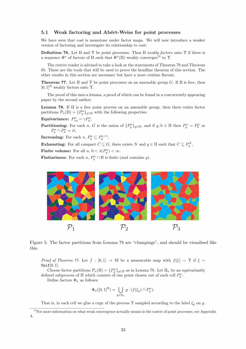
5.1 Weak factoring and Abert-Weiss for point processes

We have seen that cost is monotone under factor maps. We will now introduce a weakerversion of factoring and investigate its relationship to cost:

Definition 76. Let Π and Υ be point processes. Then Π weakly factors onto Υ if there isa sequence Φn of factors of Π such that Φn(Π) weakly converges15 to Υ.

The restive reader is advised to take a look at the statements of Theorem 79 and Theorem85. These are the tools that will be used to prove the headline theorem of this section. Theother results in this section are necessary but have a more routine flavour.

Theorem 77. Let Π and Υ be point processes on an amenable group G. If Π is free, then[0, 1]Π weakly factors onto Υ.

The proof of this uses a lemma, a proof of which can be found in a concurrently appearingpaper by the second author:

Lemma 78. If Π is a free point process on an amenable group, then there exists factorpartitions Pn(Π) = Png g∈Π with the following properties:

Equivariance: Pnγg = γPng ,

Partitioning: For each n, G is the union of Png g∈Π, and if g, h ∈ Π then Png = Pnh orPng ∩ Pnh = ∅,

Increasing: For each n, Png ⊆ Pn+1g ,

Exhausting: For all compact C ⊆ G, there exists N and g ∈ Π such that C ⊆ PNg ,

Finite volume: For all n, 0 < λ(Png ) <∞.

Finitariness: For each n, Png ∩Π is finite (and contains g).

Figure 5: The factor partitions from Lemma 78 are “clumpings”, and should be visualised likethis.

Proof of Theorem 77. Let f : [0, 1] → M be a measurable map with f(ξ) ∼ Υ if ξ ∼Unif[0, 1].

Choose factor partitions Pn(Π) = Png g∈Π as in Lemma 78. Let Πn be an equivariantlydefined subprocess of Π which consists of one point chosen out of each cell Png .

Define factors Φn as follows:

Φn([0, 1]Π) =⋃g∈Πn

g · (f(ξg) ∩ Png ).

That is, in each cell we glue a copy of the process Υ sampled according to the label ξg on g.

15For more information on what weak convergence actually means in the contxt of point processes, see AppendixA.

33

It follows immediately that Φn([0, 1]Π) weakly converges to Υ: if C ⊆ is any compactstochastic continuity set for Υ, then for sufficiently large N is is entirely contained in somePNg , and thus the point counts of Φn([0, 1]Π) inside C are exactly distributed the same asthose of Υ.

The following statement is due to Abert and Weiss [AW13] for discrete groups, we extendit to point processes:

Theorem 79. Let Π be an essentially free point process. Then it weakly factors onto [0, 1]Π,its own IID.

Proof. It suffices to show that Π weakly factors onto [d]Π, where [d] = 1, 2, . . . , d isequipped with the uniform measure, since [d]Π weakly converges to [0, 1]Π as d → ∞. Wewill do this by constructing factor [d]-labellings Cn of Π such that Cn(Π) weakly convergesto [d]Π.

To do this, we’ll use the second moment method, hewing close to the original Abert-Weissrecipe.

The strategy will be as follows. Consider the set of [d]-labellings of Π. We will studya probabilistic model that produces a random element of this space. We will show thatthis random deterministic colouring satisfies certain constraints with positive probability.In particular, there must exist a [d]-labelling satisfying those constraints. By adjusting theparameters of this model, one can produce the desired sequence Cn.

Fix a countable weak convergence determining family Vi as discussed at Lemma 135, sothat the sets Vi ⊂ G× [d] are bounded stochastic continuity sets for [d]Π. We will constructa sequence of factor colourings Cn of Π such that for fixed k,

NV k(CnΠ) converges weakly to NV k([d]Π),

where V k = (V1, V2, . . . , Vk).Set Wk =

⋃i≤k Vk to be the total window. Formally this is a subset of G × [d], but we

view it as a subset of G. For ε > 0 arbitrary, we choose δ > 0 so small that the followingproperties are true, where µ denotes the law of Π:

µ(ω ∈M | for all g, h ∈ ω ∩Wk, g 6= h implies d(g−1ω, h−1ω) > δ) > 1− ε

and

(µ⊗µ)((ω, ω′) ∈M×M | for all (g, h) ∈ (ω∩Wk)×(ω′∩Wk), d(g−1ω, h−1ω′) > δ) > 1−ε.

This is possible by essential freeness of Π: the sets in question increase as δ tends to zeroto a set of full measure.

We now construct a random colouring C of Π in the following way: let

M0 =⊔i

Di, where diam(Di) < δ.

be a partition of M0 into small measurable sets. By the correspondences we’ve described,any [d]-colouring of the sets Di corresponds to a factor colouring C : M → [d]M in thefollowing way:

C (ω) = (g, c) ∈ ω × [d] | g−1ω ∈M0 is coloured by c.

We look at such C when the Di sets are coloured uniformly at random by elements of [d].To emphasise: we are considering a distribution on deterministic colourings.

For an integral vector α = (α1, α2, . . . , αk) ∈ Nk0 , we set

Tα = ω ∈ [d]M | (NV1(ω), . . . , NVk(ω)) = α

to be the set of configurations whose point/colour statistics in Wk are prescribed by α.Note that C∗µ(Tα) is a random variable (whose source of randomness is C ).We use the second moment method to prove the existence of C such that for all α ∈ Nk0

with ‖α‖∞ ≤M ,|C∗(µ)(Tα)− [d]µ(Tα)| < ε.

34

Then any sequence of such colourings with k,M tending to infinity will witness that Πweakly factors onto [d]Π.

Exchanging order of integration allows us to express the mean of C∗(µ)(Tα) as

E [C∗(µ)(Tα)] = E[µ(C−1(Tα))]

= E[∫

M1[C (ω) ∈ Tα

]dµ(ω)

=

∫ME [1[C (ω) ∈ Tα]]dµ(ω).

Note that for ω ∈ Aδ, all pairs of distinct points g, h ∈ ω from the window Wk havethe property that g−1ω and h−1ω fall into different Di sets, and are therefore assignedindependent colours. Thus

for ω ∈ Aδ,E [1[C (ω) ∈ Tα]] = [d]µ(Tα).

As µ(Aδ) > 1− ε, it follows that

|E [C∗µ(Tα)]− [d]µ(Tα)| < 2ε.

We now work on the variance. Again, exchanging order of integration in a similar way tobefore allows us to express the mean of (C∗(µ)(Tα))2 as

E[(C∗(µ)(Tα))2

]=

∫∫M×M

E [1[C (ω) ∈ Tα1[C (ω′) ∈ Tα] dµ(ω) dµ(ω′).

By similar reasoning to before, for (ω, ω′) ∈ (Aδ × Aδ) ∩ Bδ, the colours one will see atpoints in Wk will be independent. Thus for such (ω, ω′) we have

E[(C∗(µ)(Tα))2

]= ([d]µ(Tα))

2

Note that (Aδ × Aδ) ∩ Bδ = (Aδ ×M0) ∩ (M0 × Aδ) ∩ Bδ, so by the union bound (µ ⊗µ)((Aδ ×Aδ) ∩Bδ) > 1− 3ε.

Putting this together,

Var(C∗(µ)(Tα)) = E[(C∗(µ)(Tα))2

]− (E [C∗µ(Tα)])

2< 12ε.

We now apply Chebyshev’s inequality which states that for any c > 0,

P [|C∗(µ)(Tα)− E[C∗(µ)(Tα)]| > c] <Var(C∗(µ)(Tα))

c2.

Our bounds on the mean and the variance of C∗(µ)(Tα) and the choice c = ε13 yield

P[|C∗(µ)(Tα)− [d]µ(Tα)| > ε

13 − 2ε

]< 12ε

13 .

Let Eα denote the event |C∗(µ)(Tα)− [d]µ(Tα)| < ε. Then by the union bound

P[⋂α∈Nk0‖α‖∞≤M

Eα] ≥ 1−Mkε13 .

In particular, by choosing ε sufficiently small, such a colouring exists.

Proposition 80. Suppose Π and Υ are point processes, with Π weakly factoring onto Υand Ψ(Υ) being a factor of Υ. Then Π weakly factors onto Ψ(Υ).

That is, weak factoring is a transitive notion.

Proof. We have seen that every factor map decomposes as the composition of a (coloured)thickening and a thinning. We are therefore able to reduce the problem to the case whereΨ is a thinning, a colouring, and a thickening.

35

We will repeatedly use the following fact: if Π weakly factors onto Ψm(Υ) for a sequenceof factors Ψm, and Ψm converges to Ψ pointwise, then Π weakly factors onto Ψ(Υ).

We begin with the case of thinnings.Let Φn(Π) weakly converge to Υ. We write µ and ν for the laws of Π and Υ respectively.

Let θA be a thinning of Υ, determined by a subset A ⊆ (M0, ν0) as in Theorem 55.The idea of the proof is this: if A were a ν0 continuity set, then the corresponding

thinning θA : M → M is continuous ν almost everywhere, and so θA(Φn(Π)) converges toθA(Υ) by Lemma 118. We handle the general case by approximating A by ν0 continuitysets.

Claim. If A is a ν0 continuity set, then θA : M→M is continuous ν almost everywhere.

To see this, recall the saturation notion we used in the proof of Theorem 55. We’veassumed ν0(∂A) = 0, and hence ν(G∂A) = 0 too. Then θA is continuous on the complementof this set. Note that if ω 6∈ G∂A, then g−1ω 6∈ ∂A for all g ∈ ω. One can now see thatif ωn converges to ω, then θA(ωn) restricted to any fixed radius ball is eventually equal toθA(ω), as desired.

For the general case, let Am ⊆M0 be ν0-continuity sets such that

ν0(A4Am) <1

2m.

Then for every m, we have θAm(Φn(Π))→ θAm(Υ) by our earlier argument.By Borel-Cantelli, A4Am does not occur infinitely often. This is true for the saturation,

so we see that θAm → θA pointwise almost surely and hence also in distribution. By choosingan appropriate subsequence of ms and ns we find our desired sequence of factor maps.

The above proof for thinnings can be immediately adapted to prove that Π weakly factorsonto Ψ(Υ) if Ψ is any [d]-colouring of Υ. Since any colouring is a pointwise limit of finitarycolourings, we see that Π weakly factors onto any colouring of Υ.

Finally, suppose Ψ is a thickening of Υ. By using the Voronoi tessellation we may expressΨ in the following form:

Ψ(ω) =⋃g∈ω

gF (g−1ω),

where F : M0 →M0 is a measurable function.We say that Ψ is a bounded range thickening if there exists C > 0 such that F (Υ0) ⊆

B(0, C) almost surely.It is easy to show that Ψ is the pointwise limit of such thickenings, so we are reduced to

this case.Define I : M0(B(0, C)M →M by

I(ω) =⋃g∈ω

gξg,

where ξg is the label of g in ω, that is, (g, ξg) ∈ ω.This is the implementation map: it takes a schema for a thickening and implements it.

Claim. The implementation map I is continuous.

The task is to show that given R, ε > 0 there exists S, δ > 0 such that if ω and ω′ are(S, δ)-wobbles of each other, then I(ω) and I(ω′) are (R, ε)-wobbles of each other.

The idea is simply that the behaviour of I(ω) in a ball of radius R is determined by ωrestricted to the ball of radius R+C, as the thickening is of bounded range C. By choosingδ sufficiently small (depending on the labels of the points in ω ∩ B(0, R + C), we find ourdesired S and δ.

With the claim in hand, our desired result follows from the claim and Lemma 118.

Corollary 81. Let Π and Υ be point processes on an amenable group, with Π free. ThenΠ weakly factors onto Υ.

Proof. By Theorem 79 Π weakly factors onto [0, 1]Π, and by Theorem 77 [0, 1]Π weaklyfactors onto Υ. Hence the claim follows from Proposition 80.

36

Lemma 82. Suppose Πn weakly converges to Π. Then [0, 1]Πn weakly converges to [0, 1]Π.

Proof. This can be seen, for instance, by verifying that the finite dimensional distributionsof [0, 1]Πn weakly converge to those of [0, 1]Π.

Recall that a [0, 1]-marked point process on G is just a particular kind of point processon G × [0, 1]. It therefore suffices to check weak convergence of the finite dimensionaldistributions against stochastic continuity sets of [0, 1]Π in product form.

To that end, let V = (V1, V2, . . . , Vk) denote a collection of stochastic continuity setsfor Π, and [0,p) = ([0, p1), [0, p2), . . . , [0, pk)) a family of intervals in [0, 1]. We denoteby V × [0,p) = (V1 × [0, p1), . . . , Vk × [0, pk)) the stochastic continuity set of [0, 1]Π. Fixan integral vector α ∈ Nk0 . We must show that P[NV ×[0,p)[0, 1]Πn = α] converges toP[NV ×[0,p)[0, 1]Π = α].

We find the following explicit expression simply by conditioning on β, the total numberof points appearing in V :

P[NV ×[0,p)[0, 1]Πn = α] =∑β≥α

P[NV ×[0,p)[0, 1]Πn | NV Πn = β]P[NV Πn = β]

=∑β≥α

k∏i=1

pαii (1− pi)βi−αiP[NV Πn = β],

where by β ≥ α we mean that βi ≥ αi for each entry.There is an identical expression for Π (simply replace all instances of Πn by Π). The

conclusion follows, as P[NV Πn = β] converges to P[NV Π = β] for all β.

We have seen that all free point processes are able to weakly factor onto their own IID.It is natural to ask if all this hassle was worth it – can a point process always factor directlyonto its own IID?

Theorem 83 (Holroyd, Lyons, Soo [HLS11]). The Poisson point process cannot be split intotwo independent Poisson point processes of lower intensity without additional randomness.

More precisely, there does not exist a deterministic two colouring C : (M,P)→ 0, 1Msuch that C∗P is the IID Ber(p) labelled Poisson point process for 0 < p < 1.

Example. Some point processes can factor onto their own IID, however. Note that takingthe IID of a point process is idempotent, in the sense that

[0, 1][0,1]Π ∼= ([0, 1]2)Π ∼= [0, 1]Π.

For an unlabelled example, one can simply spatially implement [0, 1]Π. That is, using themethod sketched at Proposition 71 one can find an unlabelled point process Υ (abstractly)isomorphic to [0, 1]Π, and thus [0, 1]Υ ∼= Υ.

5.2 Cost monotonicity for (certain) weak factors

In this section we will always assume G is compactly generated by S ⊂ G.

Question 84. Suppose Π weakly factors onto Υ. Is it true that cost(Π) ≤ cost(Υ)? Thatis, is cost monotone for weak factors?

This is the real theorem that we would like to prove. We are able only to prove thefollowing theorem, which implies that cost is monotone for certain weak factors:

Theorem 85. Suppose Πn is a sequence of point processes that weakly converge to Π.Then

lim supn→∞

cost(Πn) ≤ cost(Π)

holds in the following cases:

1. If there exists δ,R > 0 such that Πn and Π are all δ uniformly separated and R coarselydense.

2. If all the Πn are free and Π is δ uniformly separated.

37

Moreover, the same statements are true if the point processes have labels from a compactmark space Ξ.

We will need an auxiliary lemma, which we will use again later:

Lemma 86. Let Π be a point process with law µ. Then for all but countably many δ > 0,the δ-metric-thinning map θδ : M→M is continuous µ almost everywhere.

In particular, if Πn weakly converges to Π, then θδ(Πn) weakly converges to θδ(Π).

To prove the lemma, simply note that any δ such that BG(0, δ) is a stochastic continuityset for Π0 works.

Proof of Theorem 85. We prove (1), and then show how to reduce (2) to (1).By increasing S if necessary, we may assume diam(S) < R.Denote the distributions of Πn and Π by µn and µ respectively.We call a factor graph G a µ-continuity factor graph if it has the property that

limn→∞

−→µ0n(G ) = −→µ0(G ).

The same technique used to prove Proposition 136 shows that factor graphs of the form16

GA,V = (A × V ) ∩−→M0, where A ⊆ M0 is a µ0 continuity set and V ⊆ G is a bounded

stochastic µ continuity set, are µ-continuity factor graphs.The idea of the proof is that we will take a cheap graphing G for the limit process µ, and

use it to produce a cheap µ0-continuity graphing H . The continuity property then gives usinformation about the costs of µn, but only if we can ensure H is connected on Πn. Thisis why we assume coarse density.

Note that by outer regularity of the measure −→µ0, for every factor graph G and ε > 0there exists an open factor graph G ′ ⊇ G such that −→µ0(G ′) ≤ −→µ0(G ) + ε. Therefore in thedefinition of cost one can replace “measurable graphing” by “open graphing”.

Claim. Every open graphing G of µ contains a µ-continuity factor graph HN such that

H NN ⊇

−→M0 ∩ (Hδ × S).

Here Hδ denotes the space of δ separated configurations as in Lemma 129.Note that this condition and the assumption on R and S implies that H is connected on

any δ-uniformly separated and R coarsely dense input. In particular, H (Πn) is connectedfor every n.

To finish the proof from here: for any ε > 0, choose a graphing G of Π such that−→µ0(G ) ≤ cost(Π) + ε. Take H as in the above procedure. Then:

lim supn→ ∞

cost(Πn) ≤ lim supn→ ∞

−→µ0n(H ) as H is a graphing of Πn

= −→µ0(H ) since H is a −→µ0-continuity graphing

≤ −→µ0(G ) as H ⊆ G

≤ cost(Π) + ε by assumption on G .

Since ε > 0 was arbitrary, this proves the result.We must now prove the claim.Recall from Lemma 134 that M0 and G admit topological bases Ai and Vj consisting

of µ0-continuity sets and µ stochastic continuity sets (respectively). So by definition of the

subspace topology,−→M0 admits a topological basis GAi,Vj consisting of µ-continuity factor

graphs.For each k ∈ N define

Hk =⋃i,j≤k

GAi,Vj⊆H

GAi,Vj .

Since Hk consists of finitely many continuity factor graphs, it is itself a continuity factorgraph. Each Hk is also open, and increases to H as k tends to infinity.

16Let us unpack the definition: there is an edge between g, h ∈ GA,V (ω) if g−1ω ∈ A and g−1h ∈ A. That is,each point g decides locally if it will have edges (checks if g−1ω ∈ A), and then simply connects to all points ingV .

38

As H is generating, H kk k∈N forms an open cover of the compact space

−→M0∩ (Hδ×S).

In particular, there exists N such that H NN ⊇

−→M0 ∩Hδ × S, proving the claim.

One sees that the essential feature in the above proof strategy was compactness, andtherefore it remains true for Ξ-labelled point processes if Ξ is compact, as mentioned.

With this observation in hand, we can now deduce the (2) statement from the (1). Wewill produce a weakly convergent sequence of point processes, where each term has the samecost as Πn and the weak limit factors onto Π, thus has cost at most the cost of Π. Thisproves the statement.

Choose δ′ < δ as in Lemma 86 so that δ′ metric thinning satisfies

θδ′(Πn) weakly converges to θδ

′(Π) = Π.

Now observe by label trickery (see 74) we can find [0, 1]-labelled point processes Υn eachisomorphic to the respective Πn and such that their underlying pointset is θδ

′(Πn).

Note that Υn might not weakly converge, but it will have subsequential weak limits. Allsuch subsequential weak limits will be some kind of (possibly random) labelling of Π.

To see this, let π : [0, 1]M → M be the map that forgets labels. Thus π(Υn) = θδ′(Πn).

Since π is continuous, it preserves weak limits. Let Υ be any subsequential weak limit ofΥn, along a subsequence nk. Then by continuity

π(Υ) = limk→∞

π(Υnk) = limk→∞

θδ′(Πnk) = Π.

Now let Θn(Υn) be the input/output versions of the (δ′, R)-Delone thickenings that existfrom Proposition 69. Here we use that Υn are free actions. By input/output we mean youkeep track of which points of the thickening are input and output, as in Definition 31. Inparticular,

cost(Θn(Υn)) = cost(Υn) = cost(Πn),

where the first equality holds because we took the input/output version of the thickening.Let Υ′ denote any subsequential weak limit of Θn(Υn). Then Υ′ factors onto Π, by a

similar argument to the earlier one about forgetting certain labels. Putting this all together:

lim supn→∞

cost(Πn) = cost(Θn(Υn)) ≤ cost(Υ′) ≤ cost(Π),

where the final inequality holds because cost can only increase under factors.

Remark 87. In the second part of the proof, one might want to replace label trickery bysomething like “each Πn is isomorphic to a random Delone set Υn, which has subsequentialweak limits, so choose one such limit Υ...”, but then it’s not clear what the cost of Υ hasto do with the cost of Π. One would require the Delone-ification process to preserve weaklimits in some sense in order to relate cost(Υ) and cost(Π).

Remark 88. There is label trickery in [AW13] too: it is always assumed there that theaction is continuous on a compact space.

Theorem 89. If Π is a free point process, then its cost is at most the cost of the Poissonpoint process on G.

Proof. It is enough to prove that the IID Poisson point process [0, 1]P maximises thecost. This implies cost(P) ≤ cost([0, 1]P), and cost([0, 1]P) ≤ cost(P) by factoring, socost([0, 1]P) = cost(P).

We know that Π weakly factors onto [0, 1]Π, and [0, 1]Π factors onto the IID Poisson.We would like to say “so Π weakly factors onto the IID Poisson, and hence has less cost bythe cost monotonicity statement”, but our cost monotonicty statement is too weak for this.C’est la vie.

Note that Π is abstractly isomorphic to a δ uniformly separated process Π′ by Proposition71. Then Π′ is also free and has the same cost as Π. Now Π′ weakly factors onto its ownIID, more explicitly, there is a sequence of factors labellings Φn(Π′) weakly converging to

39

[0, 1]Π′. Because Φn(Π′) is a labelling of Π′ it is itself free and uniformly separated. Putting

it all together:

cost(Π) = cost(Π′) as they are isomorphic actions

≤ lim supn→∞

cost(Φn(Π′)) cost can only increase for factors

≤ cost([0, 1]Π′) by Theorem 85

≤ cost([0, 1]P) as [0, 1]Π′

factors onto [0, 1]P ,

as desired.

6 Some fixed price one groups

The results of the previous section immediately suggest a strategy that could be used toprove groups have fixed price one – namely, one ought to prove that the IID Poisson hasfixed price one. Even on groups of the form G×Z with G nondiscrete, we are unable to dothis directly, in the following sense:

Question 90. Can one explicitly construct for every ε > 0 connected factor graphs of theIID Poisson on G× Z of edge measure less than 1 + ε?

To see what we mean by explicit, one should consider the discrete case: if Γ is a finitelygenerated group, then it is straightforward to construct factor of IID connected graphs ofsmall edge measure on Bernoulli (site) percolation on Γ× Z. We would like a constructionin that vein.

So instead we will use the weak factoring strategy to reduce the above problem to amuch simpler one, where we can construct such factor graphs.

6.1 Groups of the form G× ZDefinition 91. Let Π be a point process onG. Its vertical coupling onG×Z is ∆(Π) = Π×Z.

Here ∆ : M(G) → M(G × Z) is induced by the diagonal embedding of G into GZ. Forthis reason one might prefer to call ∆(Π) the diagonal coupling, but this terminology willnot be suitable when we go to G× R.

Lemma 92. The IID version [0, 1]∆(Π) of a vertically coupled process has cost one.

The proof uses the fact that Bernoulli percolation of a factor graph can be implementedas a factor of IID. This sort of trick will be familiar to many, but we will nevertheless spellit out:

Definition 93. Let G be a factor graph of a point process Π. Its ε edge percolation is thefactor graph Gε defined on [0, 1]Π in the following way: for points g, h ∈ [0, 1]Π let

g ∼Gε h whenever g ∼G h and ξg ⊕ ξh < ε.

Here ⊕ denotes addition of the labels modulo one.

Observe that if (g, h1) and (g, h2) are edges of G (Π), then the random variables ξg ⊕ ξh1

and ξg ⊕ ξh2 are independent uniform once again.

Remark 94. If G is already a factor graph defined on [0, 1]Π, then we can implement Gεon [0, 1]Π, that is, without adding further randomness (via the replication trick).

Proof of Lemma 92. Let G be any graphing of Π with finite edge density. We lift it to afactor graph G ∆ of ∆(Π) in the following way:

(g, n) ∼G ∆(Π) (h, n) if and only if g ∼G (Π) h,

that is, as ∆(Π) is just copies of Π stacked on every level of G× Z, then we simply copy Gonto every level of G× Z as well.

40

Figure 6: How one should think of G×Z. Note that if Π is a point process on G, then its verticalcoupling is simply infinitely many copies of the same points stacked on top of each other.

Let V denote the factor graph of ∆(Π) consisting of vertical edges, that is for every(g, n) ∈ ∆(Π) we have an edge to (g, n+ 1).

One can see that V ∪ G ∆ is a connected factor graph. But this is also true whenwe percolate the edges level wise, that is, when we consider V ∪ G ∆

ε . This is because if(g, n) ∼G ∆ (h, n) is an edge destroyed in the percolation, then we can slide up along verticaledges and consider the edge (g, n+ 1) ∼G ∆ (h, n+ 1) instead. Its chance of survival in thepercolation is independent from the previous edge, and hence we get another go to crossover. By sliding up far enough we are guaranteed to be able to cross.

Lemma 95. Suppose Π and Υ are point processes, and Π factors onto Υ. Then [0, 1]Π

factors onto [0, 1]Υ. In particular, if [0, 1]Π weakly factors onto Υ then [0, 1]Π weakly factorsonto [0, 1]Π too.

The proof of this uses the following replication trick : note that the randomness in oneUnif[0, 1] random variable ξ is equivalent to the randomness in an entire IID sequenceξ1, ξ2, . . . of Unif[0, 1] random variables.

More precisely, there is an isomorphism17 (as measure spaces)

I : ([0, 1],Leb)→ ([0, 1]N,Leb⊗N).

So if ξ ∼ Unif[0, 1], then we will write I(ξ) = (ξ1, ξ2, . . .) for the associated IID sequence ofUnif[0, 1] random variables.

Proof of Lemma 95. Suppose Υ = Φ(Π). If g ∈ [0, 1]Π, then we write ξg for its label, and bythe replication trick ξg1 , ξ

g2 , . . . for the associated IID seqence of Unif[0, 1] random variables.

We define a factor map Φ of [0, 1]Π as follows:

Φ([0, 1]Π) =⋃

g∈[0,1]Π

(hi, ξgi ) ∈ G× [0, 1] | Vg(Π) ∩ Φ(Π) = (h1, h2, . . . , ),

where we mean that (h1, h2, . . .) is any enumeration of Vg(Π)∩Φ(Π) performed in an equiv-ariant way.

For instance, look at the elements of h ∈ Vg(Π) ∩ Φ(Π) which are closest to g. Then leth1 be the element that minimises T (g−1h), where T : G→ [0, 1] is the tie-breaking function

17One can make the isomorphism as explicit as one wishes, but it will not aid in understanding

41

of Section 50. Then let h2 be the next smallest element, and so on, until you exhaust theclosest elements. Then look at the batch of next closest elements and so on. One can checkthat this is an equivariant construction (any construction where you do the same thing atevery point will be).

Then Φ([0, 1]Π) = [0, 1]Υ, as desired.For the second part, simply note that taking the IID is idempotent in the sense that

[0, 1]([0, 1]Π) ∼= [0, 1]Π, and apply Lemma 82.

Proposition 96. The IID Poisson on G × Z weakly factors onto the vertically coupledPoisson of G.

Proof. We will construct factor maps Φn : [0, 1]M → M that “straighten” the input in thefollowing way: for a given input ω ∈ [0, 1]M, we select a “sparse” subset of its points. Ateach one of these we propagate them upwards by placing copies of them on the levels above.This will converge to a vertically coupled process for suitable inputs.

More precisely, let Π denote the (unit intensity) IID Poisson on G× Z. We will denotepoints of Π by (g, l) ∈ G× Z, and write Πg,l for its label.

We now define the factor map Φn in two stages as a thinning and then a thickening tosimplify the analysis. Let

Π1/n = (g, l) ∈ Π | Πg,l ≤1

n,

and Fn = 0 × 0, 1, . . . , n− 1. Set

ΦnΠ = ΘFn(Π1/n),

where we write ΦnΠ for Φn(Π) to conserve parentheses.Let us explain what this means:

• At the first step Π 7→ Π1/n, we independently thin Π to get a subprocess of intensity1n . By the discussion in Example 2.2, the resulting process Π1/n is simply a Poisson

point process on G× Z of intensity 1n . We refer to the points of Π1/n as progenitors.

• Each progenitor (g, l) spawns additional points with the same G-coordinate on thenext n− 1 levels above it. This is the map Π1/n 7→ ΘFn(Π1/n) = ΦnΠ.

• By the discussion at Example 2.2, ΦnΠ is a process of unit intensity.

We will employ the following strategy to show that ΦnΠ weakly converges to the verticalPoisson:

1. The sequence (ΦnΠ) admits weak subsequential limits, which a priori might be randomcounting measures,

2. These subsequential limits are actually simple point processes,

3. All of these subsequential limits are vertical processes, and

4. That process is the vertical Poisson.

Recall that if (xn) is a relatively compact sequence and every subsequential limit of (xn)is x, then xn converges to x.

By this basic fact and the above items, we can conclude that (ΦnΠ) weakly converges tothe vertical Poisson.

We now verify that ΦnΠ is uniformly tight, proving (1). It suffices to verify that thedistributions of point counts NC(ΦnΠ), where C = BG(0, r)× [L] denotes a cylinder whosebase is a ball of radius r and its height (in levels) is L, are uniformly tight.

Let Xi denote the number of points in BG(0, r) × i with label Πg,i ≤ 1n , that is, the

number of progenitors on the ith level. Thus the Xi are IID Poisson random variables withparameter λ(BG(0, r))/n.

One can explicitly describe the random variable NC(ΦnΠ) in terms of the Xis, but forour purposes it is enough to observe that:

NC(ΦnΠ) ≤ Ln∑i=1

Xi.

42

The sum of independent Poisson random variables is again Poisson distributed (withparameter the sum of the parameters of the individual Poissons), so we see that NC(ΦnΠ)is bounded in terms of a random variable that does not depend on n. Therefore ΦnΠ isuniformly tight.

To prove item (2), note that the above shows that the point counts in BG(0, r) × 0for ΦnΠ are exactly Poisson distributed with parameter λ(BG(0, r)). Thus if Υ is anysubsequential weak limit of ΦnΠ and r is such that BG(0, r)×0 is a stochastic continuityset for Υ, then NBG(0,r)×0Υ will also be Poisson distributed. In particular, Υ must be asimple point process.

For item (3), let Υ be any subsequential weak limit of ΦnΠ. Observe that Υ is verticalif and only if (g, l) ∈ Υ implies (g, l + 1) ∈ Υ. The idea is that this property is satisfied formost points of ΦnΠ, and therefore must be preserved in the weak limit. Note that a processis vertical if and only if its Palm measure is vertical almost surely.

We can now explicitly describe the Palm measure of Φn(Π). Recall from Theorem 3.2

that the Palm version Π1/n0 of Π1/n is simply Π1/n ∪ (0, 0).

To express the Palm version of the Fn-thickening of Π1/n (a la Example 3.2), it will beuseful to introduce the following notation. For each k ∈ NN , let

Π1/nk = Π

1/n0 · (0, 1) = (g, l + 1) ∈ G× Z | (g, l) ∈ Π

1/n0 .

That is, you simply shift Π1/n0 up by one level. Then Φn(Π0) = Π

1/n0 ∪Π

1/n1 · · · ∪Π

1/nn−1.

Denote by K a random integer chosen uniformly from 0, 1, . . . , n− 1. Then the Palmversion of Φn(Π) is

(ΦnΠ)0 = Π1/n−K ∪Π

1/n−K+1 ∪ · · · ∪Π

1/n−K+n−1,

where we use parentheses to stress that it is the Palm version of ΦnΠ, not Φn applied toΠ0.

Let us say that a rooted configuration ω ∈ M0(G × Z) has an ε-successor if there is apoint approximately above the root (0, 0) in ω. More precisely, we define an event

ω has an ε-successor := ω ∈M0 | NBG(0,ε)×1ω > 1.

From this, we see

P[(ΦnΠ)0 has an ε-successor] ≥ n− 1

n,

as (ΦnΠ)0 certainly has an ε-successor whenever K < n− 1.Recall that Υ was any subsequential weak limit of ΦnΠ. Fix a subsequence ni such that

ΦniΠ weakly converges to Υ.Choose a sequence εk tending to zero such that BG(0, εk)×1 is a stochastic continuity

set for Υ. This is possible by Lemma 134. Then for each k

ni − 1

ni≤ P[Φni(Π)0 has an εk-successor]→ P[Υ0 has an εk-successor],

So Υ0 has εk-successors almost surely for every k, and hence has 0-successors. That is,Υ is a vertical process, at last proving item (3).

Finally, for item (4) we observe that any vertical process is completely determined by itsintersection with G × 0. We observed in the proof of item (2) that Υ is a Poisson pointprocess on the 0th level, so it must be the vertical Poisson, as desired.

Corollary 97. Groups of the form G× Z have fixed price one.

Proof. By the previous proposition and Lemma 95, we know that the IID Poisson weaklyfactors onto the IID of the vertically coupled Poisson. Explicitly, there exists factor mapsΦn : [0, 1]M → [0, 1]M such that

ΦnΠ weakly converges to [0, 1]∆(P),

where Π is the IID Poisson on G and18 P is the Poisson on G.

18This is a slight abuse of notation: we were using P to denote the law of the Poisson point process, but inthe above expression we treat it as if it were a random variable. We do this to prevent the profusion of asterisksrepresenting pushforwards of measures.

43

Choose δ < 1 as in Lemma 86 such that metric δ-thinning preserves the weak limit. Notethat because δ < 1, the thinning commutes with the vertical coupling: that is, θδ(∆(P)) =∆(θδP). Therefore

θδ(ΦnΠ) weakly converges to [0, 1]∆(θδ(P)).

Putting this all together,

cost(Π) ≤ lim supn→∞

cost(θδ(ΦnΠ)) As cost can only increase under factors

= cost([0, 1]∆(θδ(P))) By Theorem 85

= 1 By Lemma 92.

Since the IID Poisson has maximal cost, this proves that G× Z has fixed price one.

Remark 98. With further percolation-theoretic assumptions on G, one can directly showthat cost(Φn(Π)) ≤ 1 + εn, where εn tends to zero. This is by constructing factor graphs onΦn(Π).

By using the Poisson net, one can prove an analogue of the Babson and Benjaminitheorem [BB99] and show that the distance DR factor graph on the Poisson point processon a compactly presented and one-ended group has a unique infinite connected componentif R is sufficiently large.

Now on Φn(Π), we construct a factor graph as follows: add in all vertical edges, and theDR edges horizontally. Now percolate the horizontal edges. One can show that by addinga small amount of edges to this, the result is a graph with a unique infinite connectedcomponent.

6.2 Groups of the form G× RWe now outline the modifications required to extend the G×Z case to the following theorem:

Theorem 99. Groups of the form G× R have fixed price one.

Proof. The strategy will be exactly the same as in Proposition 96.We define factor maps Φn of the IID Poisson Π using the same formula as in the G× Z

case. We claim these weakly converge to a point process Υ which is vertical in the sensethat (g, t) ∈ Υ implies (g, t+ n) ∈ Υ for all n ∈ Z.

First we show Φn(Π) is uniformly tight. This works exactly as in the G × Z case,except instead of counting progenitors Xi on G × i, we count them on G × [i, i + 1) fori ∈ Z.

Next we show that any subsequential weak limit Υ of Φn(Π) is not just a randomcounting measure, but an actual point process. This follows as in the G×Z case, as Φn(Π)has the same distribution in G× [0, 1) as a Poisson point process on G× R.

The proof that Υ is a vertical point process works the same as in the G× Z case.At this point one can observe that a vertical process is determine by its intersection with

G× [0, 1), and therefore Φn(Π) weakly converges to a unique point process Υ.We now adapt Lemma 92 to this context, and show that if Υ is any vertical point process,

then its IID [0, 1]Υ has cost one.Let π : G×R→ G denote the projection map. Observe that if Υ is vertical, then π(Υ) is

discrete, and hence defines a point process on G. For contrast, observe that the projectionπ(Π) of the Poisson point process Π is almost surely dense, and hence does not define apoint process on G.

Let19 G be a finite cost graphing of π(Υ). We lift this to a factor graph of Υ in thefollowing way:

(g1, t1) ∼H (Υ) (g2, t2) when g1 ∼G (π(Υ)) g2 and |t1 − t2| < 1.

19Technically we are assuming such a thing exists, which will be the case if π(Υ) is a free point process on G,or a lattice shift where the lattice is finitely generated.

44

Let V (Υ) denote the set of vertical edges, that is

V (Υ) = ((g, t), (g, t+ n)) ∈ Υ×Υ | n ∈ Z.

Then as in Lemma 92, the vertical edges V (Υ) together with an ε-percolation of H (Υ)defines a cheap connected factor graph of Υ.

Figure 7: A portion of a graphing on the projection of a vertical process, and how it might lookwhen lifted. Note that it gets wobbled a bit in the process.

We conclude from this that G× R has fixed price one by the same kind of reasoning asin Corollary 97.

Remark 100. The limiting process here can be described as follows: sample from a Poissonon G× [0, 1), and then simply extend it periodically in the second coordinate.

6.3 Groups containing noncompact amenable normal subgroups

Theorem 101. If a compactly generated group G admits a noncompact amenable normalsubgroup A, then G has fixed price one.

We will further assume that A is nondiscrete. Our arguments carry through in thatcase, but references to the Poisson point process must be replaced by ones to Bernoullipercolation.

Our strategy is as before: we first identify a point process on such groups with cost one,and then we show that the Poisson point process weak limits onto it.

Definition 102. Let η denote a random Borel measure on G. Then the Cox process directedby η is the Poisson point process sampled according to η.

The Poisson point process driven by a Borel measure λ exists so long as the measure isnonatomic20. The same is true for Cox processes.

Example. Suppose T > 0 is a random variable. Then one can take the Cox process directedby Tλ, where λ is the Haar measure.

20Also known as diffuse, that is, λ(x) = 0 for all points x of the space.

45

We fix Haar measures λA on A and λQ on Q = G/A respectively. These can be chosen21

so that the fundamental equation

λ(B) =

∫G/A

λgA(B)dλQ(gA)

is satisfied, where λgA the shift of the Haar measure to gA, that is, λgA(V ) = λA(g−1V ).

Example. Let Υ denote the Poisson point process on Q = G/A with respect to its Haarmeasure λQ. Define a random measure η on G by

η =∑gA∈Υ

λgA,

where we extend λgA to be a measure on G by declaring it to be zero off gA.In other words, we sample from a Poisson point process on Q, and in each resulting

coset gA we independently sample from a Poisson point process (where we identify gA as atranslate of A).

Let Ψ denote the Cox process directed by η. We show that its IID [0, 1]Ψ has cost oneby constructing cheap factor graphs.

First, fix a cost one factor graph for the Poisson point process on A. Each coset is anindependent copy of this process, so our factor graph will have those edges.

Observe that the projection ΨA ⊆ G/A is just the Poisson point process on Q. This isa compactly generated group, so there is a connected factor graph G of ΨA with finite cost.

We lift this factor graph in a similar fashion to the G ×R case – connect points (x, y) ∈ Ψif their projections xA, yA are connected in G (ΨA), and y is closest to x amongst all pointsof xA (or vice versa).

Not only is this a connected factor graph, but it remains so if we ε-percolate edges goingbetween different cosets. This can be implemented on [0, 1]Ψ, so that process has cost one.

Proposition 103. Let G be as in Theorem 101. Then the IID Poisson on G weakly factorsonto the Cox process of Example 6.3.

We will define factors of the IID Poisson in a similar way to how we handled G×Z. Weagain choose a sparse set of progenitors, and add some points local to them. They will liveon the corresponding coset of A and come from a Poisson sampled on Følner sets.

Lemma 104. Let G be an lcsc amenable group. Then for any finite family of compact setsB1, B2, . . . , Bn and any ε > 0, there exists a measurable subset F ⊆ G such that for alli ∈ [n],

λ(ViF )

λ(F )< 1 + ε.

Fix a determining class Vi as in Lemma 135. Choose Fn as in Lemma 104 with εn → 0and Bn = V −1

n Vn ∩A. We may further assume that Fn exhaust G and are symmetric.Let [0, 1]Π denote the IID Poisson on G. We define a random measure ηn as follows

ηn =∑x∈Π

ξx<1/βn

λA(xFn ∩ •), where βn = λA(Fn).

We claim that the Cox process Ψn directed by ηn weakly converges to Ψ, the Cox processdirected by η. Note that each Ψn can be implemented as a factor of the IID Poisson, so thisproves Proposition 6.3.

Our strategy for proving weak convergence will be a little different this time and requiremore point process theory.

Definition 105. Let Π be a point process on G. Its avoidance functional P0 is defined onBorel subsets of G by

P0(V ) := P[Π ∩ V = ∅].

21See Theorem 6.18 of [KEK05].

46

Theorem 106 (Renyi-Monch, Theorem 9.2.XII of [DVJ07]). The avoidance functionalcharacterises point processes up to distribution. That is, if two point processes have equalavoidance functional then they have the same distribution.

Theorem 107 (Theorem 4.18 of [Kal17]). Let Π1,Π2, . . . and Π be point processes. Fix adetermining class as in Lemma 135. Then Πn weakly converges to Π if and only if for allelements B of the determining class we have

• Pn0 (B)→ P0(B), where Pn0 is the avoidance functional of Πn and P0 that of Π, and

• lim supn→∞ ENB(Πn) ≤ ENB(Π) <∞.

Here we quote the relevant portion of the theorem as it appears in Kallenberg. It is muchmore general than we have stated, and in particular it applies to point processes which arenot necessarily invariant. Note that in our case the second condition will be redundant (asENB(Π) = λ(B) int(Π)).

Remark 108. There are subtle differences in the frameworks adopted by Kallenberg andVere-Jones, but they don’t manifest in the spaces we consider. For a detailed discussionsee [BP19].

Proof of Proposition 103. We employ the above theorem, tackling the moment conditionfirst.

By definition, NB(Ψ) is a sum of Poisson many random variables, each independent anddistributed with a random parameter. We symbolise this as follows: let

• M ∼ Pois(λQ(BA)),

• g1A, g2A, . . . be an IID sequence chosen uniformly over BA ⊆ G/A, and

• Πi be an IID sequence of Poisson point processes on giA with intensity measure λgiA.

Let V be a stochastic continuity set. By definition of the Cox process,

NV (Ψ) =

M∑k=1

|giA ∩ V |.

This sum is zero exactly when each of the summands is zero. These terms are IID, with

p := P[giA ∩ V = ∅] = E[exp(−λgA(V ))] =1

λQ(V A)

∫Q

exp(−λgA(V ))dλQ(gA).

Then

P[Ψ ∩ V = ∅] =∑k≥0

P[Ψ ∩ V = ∅|M = k]P[M = k]

=∑k≥0

(P[giΠi ∩ V = ∅])k exp(−λQ(V A))λQ(V A)k

k!

= exp(−λQ(V A))∑k≥0

(pλQ(V A))k

k!

= exp(−λQ(V A)) exp(pλQ(V A))

= exp(qλQ(V A)),

where q = 1− p as usual.An almost identical computation leads us to the expression

P[Ψn ∩ V = ∅] = exp

(qnλG(V Fn)

λA(Fn)

),

where qn = 1− pn and

pn =1

λG(V Fn)

∫V Fn

exp(−λgA(gFn ∩ V )dλG(g).

47

Our task now is to verify that

limn→∞

1

λA(Fn)

∫V Fn

exp(−λgA(gFn ∩ V )dλG(g) =

∫Q

exp(−λgA(V ))dλQ(gA).

We name the integrands in this expression as fn, f : G→ R, where

fn(g) = exp(−λgA(gFn ∩ V ) and f(g) = exp(−λgA(V )).

Note that fn converges to f uniformly on compact subsets.We name the measures in the expression too as

νn(U) =λG(U ∩ V Fn)

λA(Fn)and ν(U) = λQ(UA ∩ V A).

We claim that νn converges to ν strongly, that is, νn(U)→ νn(U) for all sets. To that end,note that

νn(U) =

∫G

λgA(U ∩ V Fn)

λA(Fn)dλQ(gA).

Here the integrand vanishes unless gA ∈ UA ∩ V A). Express g as g = ua = vα whereu ∈ U, v ∈ V and a, α ∈ A. Then

λgA(U ∩V Fn) = λuA(V Fn) = λA(u−1V Fn) = λA(aα−1v−1V Fn) = λA(v−1V Fn) ≥ λA(Fn).

Thus

νn(U) ≥∫UA∩V A

1dλQ(gA) = λQ(UA ∩ V A) = ν(U).

In the other direction our choice of Følner sets Fn yields

νn(U) =

∫UA∩V A

λA(v−1V Fn)dλQ(gA)

≤∫UA∩V A

λA(V −1V Fn)dλQ(gA)

≤∫UA∩V A

(1 + εn)dλQ(gA)

= λQ(UA ∩ V A)(1 + εn)

= ν(U)(1 + εn).

By an approximation argument one can show that

limn→∞

∫fndνn =

∫fdν,

as desired.

7 Rank gradient of Farber sequences vs. cost

Definition 109. Let (Γn) denote a sequence of lattices in a fixed group G.The sequence is Farber if for every compact neighbourhood of the identity V ⊆ G we

haveP[aΓna

−1 ∩ V = e]→ 1 as n→∞,where aΓn denotes a coset of Γn chosen randomly according to the (normalised) finite G-invariant measure on G/Γn.

Note that aΓna−1 is exactly the stabiliser of aΓn for the action G y G/Γ. Thus the

Farber condition says that the action on most points of the quotient is locally injective.Equivalently, the condition states that aΓn ∩ V a = a with high probability. It is this

second form that we will actually use in the proof below. We think of a as being a pointsampled randomly from a fundamental domain for Γn in G, and thus it states that theV -neighbourhood around this point a meets the lattice shift aΓn only trivially.

48

Definition 110. Let (Γn) denote a sequence of lattices in a fixed group G. Its rank gradientis

RG(G, (Γn)) = limn

d(Γn)− 1

covol Γn,

whenever this limit exists.

Remark 111. If G is discrete, then the Γn are all finite index subgroups. The Nielsen-Schreier formula

d(Γn)− 1

[G : Γn]≤ d(G)− 1

shows that the terms in the rank gradient are at least bounded.Gelander proved [Gel11] an analogue of this formula for lattices in connected semisimple

Lie groups without compact factors.In the Seven Samurai paper [ABB+17], it is shown that if G is a centre-free semisimple

Lie group of higher rank with property (T), then any sequence of irreducible lattices (Γn)in G is automatically Farber, as long as covol(Γn) tends to infinity.

In the particular case of a decreasing chain Γ = Γ1 > Γ2 > . . . of finite index subgroups,Abert and Nikolov showed [AN12] that the rank gradient RG(Γ, (Γn)) can be described asthe groupoid cost of an associated pmp action Γ y ∂T (Γ, (Γn)) on the boundary of a rootedtree.

Definition 112. We say that a lattice Γ < G is δ-uniformly discrete if all of its right cosetsΓa ∈ Γ\G are δ uniformly separated as subsets of G. That is, for all distinct pairs γ1, γ2 ∈ Γ,we have d(γ1a, γ2a) ≥ δ. Equivalently by left-invariance of the metric, d(e, a−1γa) ≥ δ forall γ ∈ Γ not equal to the identity e ∈ G.

If (Γn) is a sequence of lattices, then we say it is δ uniformly discrete if each Γn is δuniformly discrete in the above sense.

Theorem 113. Let (Γn) be a Farber sequence of cocompact lattices. Suppose further thatthe sequence is uniformly discrete. If its rank gradient exists, then

RG(G, (Γn)) ≤ cost(G)− 1.

In particular, if G has fixed price one then the rank gradient vanishes.

The above theorem is spiritually the same as one proved independently by Carderi in[Car18], but in a drastically different language (namely, that of ultraproducts of actions).The theorem is therefore his, but we include our own proof as it has a different flavour.In the subsequent section we will discuss a similar theorem which applies for nonuniformlattices, at least with additional assumptions on the group.

Proof of Theorem 113. Recall that the groupoid cost of a lattice shift is

gcost(Gy G/Γn) = 1 +d(Γn)− 1

covol Γn,

which is essentially the term appearing in the rank gradient definition. We would thereforelike to take a weak limit of these actions to get some free point process, and then appealto the cost monotonicity result. Of course, this is completely senseless: the intensity of thelattice shift tends to zero, so it weak limits on the empty process.

Therefore we thicken the lattice shifts to get processes Πn with a nontrivial weak limit.This thickening procedure must be done correctly, so that we can apply our (weak) costmonotonicity result.

We will produce a sequence of [0, 1]-marked point processes Πn such that

• each Πn is a 2δ-net,

• each Πn is a factor of the lattice shift aΓn, and so has cost at least 1 + d(Γn)−1covol Γn

, and

• they have a subsequential weak limit Υ with IID [0, 1] labels.

49

ThenRG(G, (Γn)) + 1 ≤ lim

n→∞gcost(Πn) ≤ cost(Υ) = cost(G)

by the cost monotonicity result, as desired.View the space of right cosets Γn\G as a compact metric space, where the distance

between two cosets Γnb1,Γnb2 ∈ Γn\G is just their distance as closed subsets of G.Let Bn = Γnbn1 ,Γnbn2 , . . . ,Γnbnkn be a collection of 2δ-nets in Γn\G, where δ is the

uniform discreteness parameter. We also choose b1 = e.This specifies a sequence of thickenings Θn of the corresponding lattice shifts: that is,

aΓn 7→ aBn.Note that Θn(aΓn) is a 2δ-net: it’s true that d(aΓnb

ni , aΓnb

nj ) = d(Γnb

ni ,Γnb

nj ) ≥ δ for

i 6= j by our choice of Bn, and points of Γnbni are uniformly separated too exactly by our

uniform discreteness assumption. It is also 2δ-coarsely dense, by the same property for Bn.Since Θn(aΓn) is a collection of random 2δ-nets, it is automatically uniformly tight,

and all subsequential weak limits are 2δ-nets (and in particular, simple point processes).At this point we could consider the input/output version of Θn (so that the image process

is weakly isomorphic to the original, and in particular has the same groupoid cost), and thenpass to a subsequential weak limit. Our issue here is that one would have to demonstratethat this weak limit is a free action in order to compare its cost to the cost of the ambientgroup. To do this, one would have to use the Farber condition in an essential way.

We bypass this by a labelling trick: note that the IID of any point process is automaticallya free action (as any two points of it will receive distinct values almost surely, killing anypossible symmetries). So we will limit on an IID labelled process instead.

Consider the action G y G/Γn × [0, 1], where the action on the second coordinate istrivial. We refer to this as the periodic IID lattice shift. It is our familiar friend the latticeshift, but with every point of it receiving the same IID label. This is of course distinct fromthe IID of the lattice shift. We write (aΓn, ξ) for a sample from this space.

Now we thicken as before, but this time distribute labels: let

Θn(aΓn, ξ) =

kn⋃i=1

aΓnbni × ξi,

where ξ1, ξ2, . . . is an IID sequence of Unif[0, 1] random variables produced as a factor of ξ.In other words, each point of the lattice shift adds points to the space and gives them

an IID [0, 1] label (but note that each point starts with the same label ξ, so this is not theIID of the thickening).

Let Υ denote any subsequential weak limit of Θn(aΓn, ξ), and pass to that subsequence.Then π(Θn(aΓn, ξ) weakly converges to π(Υ), as the projection π : G × [0, 1] → G thatforgets labels is continuous.

Our task is to show that Υ = [0, 1]π(Υ).The idea of the proof is the following: fix C ⊆ G to be a bounded stochastic continuity set

for Υ. We want to prove that the labels of the points of Θn(aΓn, ξ) in C are independent anduniform on [0, 1]. They are already Unif[0, 1] by definition, so we must now consider theirdependencies. Again, by definition, points of C arising from distinct aΓnb

ni are automatically

independent. The only dependency issue that can arise is when aΓnbni ∩ C has multiple

points. We will show that this is a vanishingly rare event.This will be achieved via the following lemma:

Lemma 114. Let C ⊆ G be compact. If (Γn) is a Farber sequence and Bn ⊆ G is anysequence of finite subsets, then P[∃b ∈ Bn such that |aΓnb ∩ C| > 1]→ 0.

Proof. Apply the Farber condition with any set V containing CC−1. If b ∈ Bn is such thatthere are aγ1, aγ2 distinct elements of aΓnb ∩ C, then

(aγ1b)(aγ2b)−1 = aγ1γ

−12 a−1 is in CC−1,

so aγ1γ−12 a−1ab = aγ1γ

−12 b ∈ V ab, and this element is also in aΓnb. By the Farber condition,

aΓnb ∩ V ab = ab

50

with high probability, and so

P[∃b ∈ Bn such that |aΓnb ∩ C| > 1] ≤ P[aΓna−1 ∩ V = e]→ 0,

finishing the proof of the lemma.

Let V = (V1, V2, . . . , Vk) denote a collection of bounded stochastic continuity sets forΥ, and [0,p) = ([0, p1), [0, p2), . . . , [0, pk)) a family of intervals in [0, 1]. We denote byV × [0,p) = (V1 × [0, p1), . . . , Vk × [0, pk)) the stochastic continuity set of [0, 1]Υ.

Let C be a compact set large enough to contain⋃i Vi.

On the event from the lemma,

NV (Θn(aΓn, ξ)) = NV ([0, 1]Θn(aΓn),

where by Θn(aΓn) we simply mean (Θn(aΓn, ξ)) with the labels erased.Therefore Θn(aΓn, ξ) converges weakly to [0, 1]Υ, finishing the proof.

7.1 Farber sequences in semisimple Lie groups

We wish to extend Theorem 113 to cover more cases of Farber sequences. Let us note theessential features of the argument:

• The lattice shifts have a sequence of factors which weakly converge to a net,

• That the sequence is Farber, so that the distributing randomness argument works togive an IID weak limit,

• Crucially, that cost monotonicity holds for a sequence of nets converging to a net.

The first two points are flexible. It is the third which causes us grief. In particular, weare unable to prove (or disprove) the following statement: suppose Πn is a sequence of finitecost point processes that weakly converge to a random net Π. Is it true that

lim supn→∞

cost(Πn) ≤ cost(Π)?

In the absence of such a statement, we content ourselves with Theorem 6.We will use the geometric interpretation of being a Farber sequence – specifically, see

Corollary 3.3 of [ABB+17]. In brief, it means that for all r > 0 the injectivity radius ofa randomly chosen point of the quotient manifold Mn = Γn\X is larger than r with highprobability, where X = G/K denotes the symmetric space of G. We will also heavily callupon the paper [Gel11].

Proof of Theorem 6. Let us denote by aΓn the lattice shift corresponding to Γn < G.

Claim. There exists a sequence Φn(aΓn) of factors are uniformly separated and have anonempty subsequential weak limit. Moreover, any such weak limit is a random net.

Unlike in the cocompact case, we cannot necessarily ensure that the factors will bethickenings.

Proof of claim. The factors will be of the form Φn(aΓn) = aΓnFn, where Fn is a finitesubset of G. By left-invariance of the metric, we can essentially view Φn as a subset of thequotient manifold Γn\X. The factor map Φn will be α-separated if ΓnFn is contained in theα-thick part of the quotient manifold. Here we choose α = α(G) as in [Gel11] (a constantdepending only on the ambient group, not on the particular lattice). Then Φn(aΓn) admitssubsequential weak limits by uniform separation, and these will be non-empty provided thattheir intensity is bounded away from zero.

We choose Fn as in Corollary 2.13 of [Gel11]. It follows from the definition of ψ0(Γn)(see page 242 of [Gel11]) that ψ0(Γn) contains all points with injectivity radius larger thanmaxε, ε2µ. In particular, by the Farber condition a randomly chosen point of Γn\X will

lie in ψ0(Γn) with high probability. The union of the α-balls centred at Fn covers ψ0(Γn),so the intensity of Φn(aΓn) is strictly bounded away from zero, as desired.

51

Finally, any subsequential weak limit of these processes must be a net: it’s certainlyuniformly separated, and

P [d(0,Φn(aΓn) < R]→ 1,

and this property is inherited by the limit.

Similar to before, we distribute randomness from the Γn-periodic IID processes. Callthe resulting process Πn. By passing to a subsequential weak limit, we can assume that Πn

weakly converges to some process Υ. As before, the Farber condition ensures that Υ is infact an IID labelled process (and in particular, its cost is at most the cost of the Poissonpoint process).

Our final task is to relate the cost of the Πn processes to the cost of Υ. We write µn0 forthe Palm measure of Πn and µ0 for the Palm measure of Υ.

By the proof of Theorem 85, any factor graph which ε-computes the cost of Υ containsa µ0-continuity factor graph G which is connected for Υ. Thus

lim supn→∞

−→µn0 (G ) ≤ −→µ0(G ).

There is no reason to expect that G is a connected factor graph for any Πn, however. Ourtask is to show that we can add a vanishingly small amount of edges to G (Πn) and connectup the process.

By construction, the graphing G has the property that there exists a constant N suchthat GN (ω) ⊇ DR(ω) for all nets ω. This is asymptotically inherited in the Palm measuresof Πn, in the sense that is,

P[0 is connected to x in G (Πn0 ) for all x ∈ B(0, R) ∩Πn

0 ]→ 1.

The complement of this set is asymptotically negligible, so at each of those points we simplyadd their DR neighbourhood. This increases the edge measure by an asymptotically neg-ligible amount (since the processes are uniformly discrete). Call the resulting factor graphGn. Then

lim supn→∞

−→µn0 (Gn) ≤ −→µ0(G ).

Finally, Gn(Πn0 ) is a connected graph – it contains DR(Πn

0 ), which is connected by Corollary2.13 and Lemma 2.14 of [Gel11].

A Metric properties of configuration spaces and weakconvergence

The following fact is the most basic requirement for a well-behaved probability theory:

Theorem 115 (See Theorem A2.6.III of [VJ03]). If X is a complete and separable metricspace, then M(X) is a Borel subset of a complete and separable metric space M#(X), andis thus a standard Borel space.

Note that configurations ω ∈ X can be viewed as measures on X, by defining ω(A) =|ω ∩A|. So configurations form particular examples of locally finite measures on X, andM#(X) will be the space of such measures. In this language, a point process is a particularexample of a random measure. Probabilists are interested in other examples of random mea-sures22, and have thus developed a framework suitable to handle all their cases of interest.We adopt their framework with small notational modifications.

We assume the reader is at least passingly familiar with weak converge of measures onmetric spaces. Recall:

Definition 116. Let M(X) denote the space of totally finite measures η on X, that is,those with η(X) <∞.

The Prokhorov metric dprok on M(X) is

dprok(η, η′) = infε ≥ 0 | for all Borel A ⊆ X, η(A) ≤ η′(Aε) + ε and η′(A) ≤ η(Aε) + ε,22And, for that matter, non-invariant point processes.

52

where Aε is the ε-halo of A, that is,

Aε = x ∈ X | d(x,A) < ε.

If η is a totally finite measure on X, then a η-continuity set is a subset A ⊆ X with theproperty that η(∂A) = 0, where ∂A denotes the topological boundary of A.

A sequence of totally finite measures ηn weakly converges to η if either of the followingconditions hold:

WC1 for all continuous and bounded functions f : X → R,

limn→∞

∫X

f(x)dηn(x) =

∫X

f(x)dη(x).

WC2 for all η-continuity sets A ⊆ X,

limn→∞

ηn(A) = η(A).

Remark 117. The Prokhorov metric metrises this convergence notion (that is, ηn convergesweakly to η if and only if dprok(ηn, η) converges to zero).

The equivalence of WC1 and WC2 is usually referred to as the Portmanteau theorem.The definition involving continuity sets will have preeminence for us. To explain the

name: note that the indicator function 1A : X → 0, 1 is continuous η almost everywhereif and only if A is an η-continuity set.

We often make use of the following well-known fact:

Lemma 118. If Φ : X → Y is a continuous map of metric spaces, then Φ preserves weaklimits: if µn is a sequence of Borel probability measures on X weakly converging to µ, thenΦ∗µn weakly converges to Φ∗µ.

Moreover, the same is true if Φ is merely continuous µ almost everywhere.

Proof. The first statement is immediate: if f : Y → R is a continuous and bounded function,then f Φ : X → R is continuous and bounded as well, so

limn→∞

∫Y

fdΦ∗µn = limn→∞

∫X

f Φdµn =

∫X

f Φdµ =

∫Y

fdΦ∗µ.

For the second statement we work with the definition involving continuity sets. Let A ⊆Y be a Φ∗µ continuity set, that is, assume µ(Φ−1(∂A)) = 0. Let DΦ = x ∈ X |Φ is discontinuous at x denote the discontinuity set of Φ. One can show that for anyA ⊆ Y that ∂Φ−1(A) ⊆ Φ−1(∂A) ∪DΦ, and so

µ(∂Φ−1(A)) ≤ µ(Φ−1(∂A)) + µ(DΦ) = 0,

that is, Φ−1(A) is a µ-continuity set. Therefore

limn→∞

Φ∗µn(A) = limn→∞

µn(Φ−1(A)) = µ(Φ−1(A)) = Φ∗µ(A),

as desired.

Definition 119. Let M#(X) denote the space of boundedly finite measures, that is, thoseBorel measures η on X that are finite on metrically bounded subsets of X.

Fix a basepoint x0 ∈ X. Let

η(r)(A) := η(A ∩B(x0; r))

denote the restriction of a boundedly finite measure η to the r-ball about x0. Note that η(r)

is therefore an element of M(X).We now define a metric d# on M#(X):

d#(η, η′) =

∫ ∞0

e−rdprok(η(r), η′(r))

1 + dprok(η(r), η′(r))dr.

A sequence of boundedly finite measures ηn weak-# converges to η if any of the followingconditions hold:

53

WHC1 for all continuous and bounded functions f : X → R which vanish outside abounded set,

limn→∞

∫X

f(x)dηn(x) =

∫X

f(x)dη(x).

WHC2 for all bounded η-continuity sets A ⊆ X,

limn→∞

ηn(A) = η(A).

WHC3 there exists a sequence rk of radii increasing to infinity such that for every k ∈ N

η(rk)n converges weakly to η(rk).

Remark 120. The space we’ve defined is obviously extremely metrically dependent (recallthat every metric is topologically equivalent to a bounded metric). However, our case ofinterest is proper left-invariant metrics on locally compact groups, which are all coarselyequivalent and thus have a well-defined notion of metrically boundedness.

We have also fixed an arbitrary base point x0. If one chooses a different basepoint x′0,then the resulting metrics will be bilipschitz equivalent.

In case X is locally compact, then weak-# convergence is equivalent to vague conver-gence.

Theorem 121. The spaceM#(X) equipped with the d# metric is complete and separable.Its Borel structure is exactly such that the mass measuring23 functions NA : X → N0 ∪∞given by η 7→ η(A) are measurable, where A is an arbitrary Borel subset of X.

Remark 122. The Borel structure on M#(X) can be generated by an even smaller col-lection of mass measuring functions: one only needs to look at NA where A ranges over asemiring of bounded Borel sets that generate the Borel structure on X.

We will require the following more explicit explanation of what weak-# convergence is:

Definition 123. Let ω ∈ M(X) be a configuration. We call another configuration ω′ ∈M(X) a (ε,R)-wobble of ω (where ε,R > 0 are some parameters) if ω(R) is in bijection

with ω′(R)

, and moreover this bijection σ : ω(R) → ω′(R)

can be chosen in such a way thatd(x, σ(x)) < ε for all x ∈ ω(R).

One direction of the following lemma is immediate, the converse is less elementary andcan be found in [VJ03] as Proposition A2.6.II:

Lemma 124. A sequence of configurations ωn converges to ω with respect to d# if andonly if there are sequences εn → 0 and Rn → ∞ such that each ωn is a (εn, Rn)-wobble ofω.

We can now discuss weak convergence of point processes. View M(X) as a subset ofM#(X) equipped with the d# metric, and recall that a point process is a probability measureon M(X). This is what we mean by a sequence of point processes weakly converging.

Note that the weak limit of a sequence of point processes µn will (a priori) be a probabilitymeasure on M#(X), not on M(X). That is, a point process might converge to a randommeasure which is not a point process. It’s easy to see that the only thing that can go wrongis mass accumulation: the limit measure will be a random atomic measure, but some atomsmight have mass larger than one.

Definition 125. A counting measure on X is a measure η with η(A) ∈ N0 for all boundedBorel subsets A ⊆ X. A simple counting measure is a measure η with η(x) = 0 or 1 forall x ∈ X.

If η is a counting measure, then its support is support(η) = x ∈ X | η(x) > 0. Thatis, support(η) is η with the multiplicities removed.

23Earlier we called these “point counting” functions, because that’s a more suitable name when the measureis atomic.

54

Example. Let Xkk∈Z denote an IID sequence of uniform [0, 1] random variables. Considerthe following sequence of point processes:

Πn = Z ∪ k +Xk

n.

In words: take two copies of Z, where you wobble all the points of one copy by smallerand smaller amounts (this is not a point process proper in our sense, as it is not invariant,but one can take a uniform [0, 1] shift of Πn if one insists).

Then Πn weakly converges to the deterministic measure µ given by µ(A) = 2|A ∩ Z|.

Remark 126. In this language, what we’ve been calling point processes are random simplecounting measures, and the comment above states that the weak limit of random simplecounting measures, if it exists, will be a possibly non-simple random counting measure.

In the literature one sometimes sees random counting measures referred to as “pointprocesses”, and random simple counting measures as “simple point processes”.

Definition 127. Let (X, d) be a csms, and (µn) a sequence of Borel probability measureson X. The sequence is uniformly tight if for every ε > 0 there exists a compact set K ⊆ Xsuch that µn(X \K) < ε for all n ∈ N.

Recall from Prokhorov’s theorem that a sequence (µn) is uniformly tight if and only ifits closure (µn) is compact.

There is a more explicit form of uniform tightness that we will use repeatedly:

Theorem 128 (See Proposition 11.1.VI of [DVJ07]). Suppose X is a locally compact24

csms. A sequence of point processes (Πn) on X is uniformly tight if and only if for everyclosed ball B ⊆ X and any ε > 0 there exists an M > 0 such that

P[NBΠn > M ] < ε for all n ∈ N.

Lemma 129. Let

Hδ = ω ∈M(X) | d(x, y) ≥ δ for all distinct x, y ∈ ω

denote the space of δ-uniformly-separated configurations. Then Hδ is compact in M(X).

Probabilists often refer to such configurations as hard-core, hence our choice of letter.The previous lemma is proved using the following basic fact:

Lemma 130. Let (X, d) denote a compact metric space. Then for all δ > 0 there existssome C > 0 such that |A| ≤ C for any δ-separated subset A ⊆ X.

The above discussion has been rather abstract. We now outline an equivalent interpre-tation of weak convergence that will be much more useful in certain applications.

Definition 131. Let Π be a point process with law µ. A stochastic continuity set of Π is aBorel subset V ⊆ G of the ambient space such that P[Π ∩ ∂V 6= ∅] = 0. Equivalently, it isa subset such that its point counting function NV : M→ N0 ∪ ∞ is continuous µ almosteverywhere.

Let V = (V1, V2, . . . , Vk) denote a collection of stochastic continuity sets for Π.The finite dimensional distributions of Π are the random vectors

NV (Π) = (NV1Π, NV2

Π, . . . , NVkΠ),

where V runs over all possible collections of stochastic continuity sets.

Remark 132. The sets

ω ∈M | NV (ω) = α, where α = (α1, α2, . . . , αk) ∈ Nk0

should be thought of as analogous to the cylinder sets in the space 0, 1Γ, where Γ is adiscrete group.

24There is a slightly more complicated version of the theorem for general Polish spaces, but we will not use it,so do not state it.

55

Note that if V is a family of stochastic continuity sets for Π, then NV is continuous µalmost everywhere. Thus by the earlier fact on weak limits and continuous functions, we seethat weak convergence of point processes implies weak convergence of the finite dimensionaldistributions. The surprising fact is that the converse is true:

Theorem 133 (See Theorem 11.1.VII of [DVJ07]). A sequence Πn of point processes weaklyconverges to Π if and only if for all collections V = (V1, V2, . . . , Vk) of stochastic continuitysets of Π, the finite dimensional distributions NV (Πn) weakly converge to NV (Π).

For this to make any sense at all, it must be the case that the finite dimensionaldistributions determine a point process. That is, if two point processes Π and Π′ have

NV (Π)d= NV (Π′) for all collections of stochastic continuity sets V , then Π

d= Π′. This is

proved using the following lemma, which states that there is an abundance of continuitysets:

Lemma 134. Let Π be a point process with law µ. Then

• for all g ∈ G, there are at most countably many r > 0 such that the open ball BG(g, r)is not a stochastic continuity set of Π, and

• for all ω ∈M, there are at most countably many r > 0 such that the open ball BM(ω, r)is not a µ continuity set.

In particular, both G and M admit topological bases consisting of µ stochastic continuitysets / µ continuity sets (respectively).

Proof. The method is the same in both cases, so we only write the proof for the firststatement. The idea of the proof is that that there cannot be so many stochastic continuitysets, else local finiteness will be contradicted. It is enough to prove that for every r > 0 andε > 0 there exists only finitely many r1, r2, . . . in (0, r) such that

P[Π ∩ ∂B(0, ri) 6= ∅] > ε for all i.

Suppose not. That is, suppose we have r, ε > 0 and infinitely many rn ⊂ (0, r)satisfying the above equation. Then

ε ≤ lim supn→∞

P[Π ∩ ∂B(0, rn) 6= ∅] ≤ P[lim supn→∞

(Π ∩ ∂B(0, rn) 6= ∅)

].

Recall that the lim sup of a sequence of events is the event that they occur infinitely often.So we see

Π ∩ ∂B(0, rn) 6= ∅ for infinitely many n ⊆ |Π ∩B(0, r)| =∞.

We’ve shown that with positive probability, Π has infinitely many points in B(0, r), a con-tradiction by local finiteness.

Note that the continuity sets form an algebra, and the cylinder sets ω ∈ M | NV (ω) =α are continuity sets when V is a collection of stochastic continuity sets. As a measure isdetermined by its values on any algebra that generates the Borel sigma algebra, we thereforesee that point processes are determined by their finite dimensional distributions. With abit more work (see [VJ03] Proposition A2.3.IV and [DVJ07] Corollary 11.1.III, Theorem11.I.VII), one can prove:

Lemma 135. Let Π be a point process. Then there exists a countable family Vii∈N ofmetrically bounded and disjoint Borel subsets Vi ⊆ G such that Πn weakly converges to Πif and only if NV Πn weakly converges to NV Π were V ranges over all finite subcollectionsof Vi.

In particular, weak convergence can be verified by a countable collection of statements,each of which only requires one to observe the process in compact windows.

The following lemma is a simpler case of Exercise 13.2.2 in [DVJ07], and is presumablyknown with a more elegant proof. The technique will be used for a later proof, so we includeit.

56

Proposition 136. Suppose µn is a sequence of finite intensity point processes that weaklyconverge to a finite intensity process µ. Then the Palm measures µn0 weakly converge to µ0.

Proof. Let A ⊆ M0 be a µ-continuity set, and U ⊆ G a stochastic µ continuity set of unitvolume. Recall that

µ0(A) =1

intµEµ[#g ∈ U | g−1ω ∈ A

]Claim. For every k ∈ N, the function ω 7→ max#g ∈ U | g−1ω ∈ A, k is continuous µalmost everywhere.

This function can only be discontinuous on the boundary of

A(l) = ω ∈M | #g ∈ U | g−1ω ∈ A = l.

Note that the claim applied with A = M0 together with the monotone convergencetheorem proves in particular that

limn→∞

intµn = intµ,

using the definition of weak convergence involving integrals of continuous bounded functions.The same sort of argument proves the proposition itself.

Observe that

µ0(∂A) = 0 By assumption, so

µ0([∂A]) = 0 As saturations of null sets are null in a countable groupoid,

µ(G∂A) = 0 By Proposition 52.

We show that ∂A(l) ∩ N∂Uω = 0 ⊆ G∂A for all l ≥ 1, establishing the claim.Suppose ω ∈ ∂A(l)∩N∂Uω = 0. Then we can find two sequences ωn, ω

′n both converging

to ω such that ωn ∈ A(l) and ω′n 6∈ A(l) for every n ∈ N. We take these to be (εn, Rn)-wobblesof ω.

We see that (for large n) the configurations ω, ωn, ω′n are all approximately equal inside

U . See Figure A.

We will refer to the points g ∈ U ∩ ω such that g−1ω ∈ A as A-points of ω and likewisefor ωn and ω′n.

Now for every (large) n, the number of A points of ωn in U is l, and the number of Apoints of ω′n in U is some (bounded) number other than l. Since the configurations are asmall wobble of ω then, we can find gn ∈ ω∩U such that the corresponding points xn of ωnand yn of ω′n are an A point and not an A point, respectively.

57

As gn ranges over a finite set ω ∩ U , we can choose g ∈ ω ∩ U and a subsequence (nk)such that gnk = g for every k ∈ N. Then

x−1nkωnk → g−1ω, and y−1

nkω′nk → g−1ω,

which witnesses that g−1ω ∈ ∂A, so ω ∈ G∂A, as desired.

B The rerooting groupoid for homogeneous spaces

One must also investigate point processes on the homogeneous spaces of groups. The setupwhich we will consider is the action of G on X = G/K, where K ≤ G is a compact subgroup.This covers the case of Riemannian symmetric spaces (such as Isom(Hd) y Hd).

Our starting point is to note that such spaces enjoy the properties we’ve been using25:namely, an invariant proper metric that makes X an lcsc space and a G-invariant Borelmeasure λX on X.

For the metric on X, one takes the Hausdorff metric:

dX(aK, bK) = max supk1∈K

infk2∈K

d(ak1, bk2), supk2∈K

infk1∈K

d(ak1, bk2),

and for the measure λX one takes the pushforward π∗λ, where π : G → X is the quotientmap a 7→ aK.

It should be clear that there will be a cost theory for such point processes. It turns outthat our existing theory carries over to the case of point processes on such homogeneousspaces with only a few small modifications, which we will discuss.

Note that because of the mapping theorem26, the Poisson point process on G maps tothe Poisson point process on X. It is intuitive that this should lead to an inequality oncosts, and we detail how this works.

Our study splits into two cases, according to if K is Haar null or not (for G’s Haarmeasure, of course). If λ(K) > 0, then by Steinhaus Theorem27 we have that K is open,and hence a compact clopen subgroup of G. It will then also have countable index. Thissituation occurs for instance in the study of Cayley-Abels graphs of totally disconnectedlocally compact groups. We will instead focus on the case that λ(K) = 0.

One can consider G-invariant point processes Π on X, which should be understood asrandom elements of M(X) whose distribution is G-invariant. We may define the intensityof Π as before:

int(Π) =1

λX(U)E|Π ∩ U |,

where U ⊆ X is any set of unit volume.One can further consider notions of thinnings, partitionings, cost, and so on. We follow

our previous strategy of studying these by looking at the associated groupoid. Let us write0 for the element K ∈ X, which we view as the root of the space. Accordingly we will definethe space of rooted configurations in X as

M0(X) = ω ∈M(X) | 0 ∈ ω.

Note that the orbit equivalence relation of G y M(X) no longer restricts to M0(X) toan equivalence relation with countable classes. The solution to this problem is to take aquotient:

25The limiting factor here is really the metric: a G-invariant Borel measure exists on G/H in fairly greatgenerality (it is an imposition on the modular functions of G and H, but an invariant metric will only exist ifG/H is homeomorphic (in an appropriate sense) to a quotient G′/H ′ with H ′ compact in G, see [AD13] forfurther details

26The mapping theorem states that if X is a space with σ-finite measure λ, Π is the Poisson point process withintensity measure λ, and f : X → Y is a measurable function, then f(Π) is the Poisson point process on Y withintensity measure f∗λ, assuming this measure has no atoms. See Section 2.3 of [Kin93] for further details.

27It states that if A ⊂ G is a subset of a locally compact group with positive Haar measure, then AA−1 containsan identity neighbourhood.

58

Proposition 137. Let K act on M0(X) by left multiplication. Then the action is smooth,that is, the space of orbits K\M0(X) is a standard Borel space.

It is a general fact that compact groups always act smoothly on standard Borel spaces(see Proposition 2.1.12 of [Zim84] and its corollary), but it is possible to give a direct proofin this case. The proof is very reminiscent of the section “Extension to more general pointprocesses” of [HP03].

Proof. We will construct a function F : M0(X)→ [0, 1] with the property that F (ω) = F (ω′)if and only if ω′ ∈ Kω. This is a characterisation of smoothness.

Fix a family Un of open subsets of G with the property that it separates M0(X) in thesense that |ω ∩ Un| = |ω′ ∩ Un| for all n if and only if ω = ω′.

Let f : 0, 1N → [0, 1] be any continuous injection, and consider the map F : M0(X)→[0, 1] given by

F (ω) = infk∈K

f((1[Un ∩ k · ω 6= ∅])n)

Note that the component functions ω 7→ 1[Un ∩ω 6= ∅] are lower semicontinuous, so theinfimum exists.

The function is constant on K-orbits by definition, but by the separating nature of thefamily Un it also takes distinct values for orbits in distinct orbits.

A Borel thinning θ : M(X)→M(X) corresponds to a Borel subset A ⊆K\ M0(X). Notethat the latter can be identified with a subset of M0(X) which is K-invariant in the sensethat KA = A, we will make such identifications freely.

To see why this K-invariance is required, consider the formula

θA(ω) := gK ∈ ω | g−1ω ∈ A.

For this to be well-defined, we need that the condition does not depend on our choice ofcoset representative gK. This is exactly asking for K-invariance of A.

In the same way one can see that Borel factor [d]-colourings correspond to Borel partitionsof K\M0(X) indexed by [d], and so on.

If Π is a G-invariant point process on X with law µ, then we may use the above to defineits Palm measure µ0 on K\M0(X) as before:

µ0(A) :=int θA(Π)

int Π

=1

int ΠE[#gK ∈ U | g−1ω ∈ A

], where U ⊆ X has unit volume.

We equip K\MK(X) with the following rerooting equivalence relation:

Kω ∼R Kω′ if and only if ∃aK ∈ ω such that Kω′ = Ka−1ω.

We can also define a groupoid structure. If one defines

−→M0(X) = (ω, aK) ∈M0(X)×X | aK ∈ ω,

then there is a natural diagonal action of K on−→M0(X). The quotient is again standard

Borel, we denote it K\−→M0(X).

Then (K\M0(X) and K\−→M0(X)) form the unit space and arrow space (respectively) of

a groupoid, which we call the rerooting groupoid. The source and target maps are definedas before

s, t : K\−→M0(X)→ K\M0(X),

s(Kω,KaK) = Kω,

t(Kω,KaK) = Ka−1ω.

A pair of arrows (Kω,KaK), (Kω′,KbK) ∈ K\−→M0(X) are deemed composable if Kω′ =

Ka−1ω, in which case

(Kω,KaK) · (Kω′,KbK) := (Kω,KabK).

59

We can equip this groupoid with the Palm measure, resulting in a r-discrete pmpgroupoid as before.

Definition 138. Let Π be a G-invariant point process on X. Its groupoid cost is

costX(Π)− 1 = infG

1

2E

[ ∑x∈U∩Π

degx G (Π)

]− int(Π),

where U is a set of unit volume in X and the infimum is taken over all connected equivariantlydefined factor graphs of Π.

The cost of X is

cost(X) := infcostX(Π) | Π is an invariant free point process on X.

Aside from replacing M0(G) with K\M0(X), our earlier arguments apply verbatim andprove the following:

• If Φ : M(X) → M(X) is a G-equivariant factor map, then costX(Π) ≤ costX(Φ(Π)).In particular, costX(Π) only depends on the isomorphism class of Π,

• Every free point process weakly factors onto its own IID,

• The Poisson point process on X has maximal costX amongst X processes.

Theorem 139. If Π is a free point process on X, then its costX is equal to its cost as aG-action.

Recall that the cost of a free pmp action of G is defined by picking an isomorphicrepresentation of the action as a point process, and taking the cost of that.

This theorem will employ a “whittling” construction. Note that we can view pointprocesses on X as random closed subsets of G (which happen to be unions of cosets of afixed compact subgroup). We are able to exploit freeness to deterministically whittle thisrandom closed subset to a point process:

Proposition 140. If Π is a free point process on X, then it admits a deterministic lift toG: that is, there exists an invariant point process Υ = Υ(Π) on G such that

• Υ ⊂ Π almost surely,

• Υ intersects each coset aK at most once, and

• π(Υ) = Π.

In other words, we are able to select one element out of every coset aK ∈ Π in anequivariant and deterministic way.

Proof of Theorem 139. Observe that the process Υ from Proposition 140 is isomorphic toΠ, so cost(Π) = cost(Υ). We verify that cost(Υ) = costX(Π). Note that factor graphs ofΠ and Υ can be bijectively identified, and so will have the same edge measures. All that isleft is to check that they have the same intensity.

For this, we use an alternative description of the measure λX on X. Fix a Borel transver-sal of K in G: this is a Borel subset T ⊆ G such that TK = G and tK ∩ sK = ∅ for alldistinct t, s ∈ T – such transversals always exist, see [FG68].

Then we can bijectively identify X with T , and under this identification the measure λXis identified with the measure λ(• ∩ T ).

In particular, if U ⊆ T has unit volume, then so too does π(U), and since

|π(U) ∩Π| = |U ∩Υ| almost surely

we have int(Π) = int(Υ), as desired.

We will require a simple lemma, which essentially already appears in Lemma 72 but weisolate for clarity. It works for point processes on G and on X.

Lemma 141. A point process Π is free if and only if it admits a deterministic labelling by[0, 1] such that all of the labels are distinct (almost surely).

60

Proof. Clearly if such a labeling exists, then the process must be free.For the converse, let I : M0 → [0, 1] be a Borel isomorphism. Define a labelling by

L : M→ [0, 1]M

L(ω) = (x, I(x−1ω) | x ∈ ω.

Observe that two distinct points x, y ∈ ω receive the same label in L(ω) exactly whenI(x−1ω) = I(y−1ω), and so xy−1ω = ω. If the process is free, then this never occurs, asdesired.

To run the proof on X, simply replace M0 by L\M0(X).

Proof of Proposition 140. By virtue of being free, we may use Proposition 71 to fix anisomorphism of Π with a point process Π′ on G. The desired process Υ will be the result ofpushing the points of Π′ into Π.

Of course Π′ is itself a free process, so we may fix a deterministic labelling L(Π′) of itspoints a la Lemma 141.

Assign each coset aK of Π to a point of x of Π′ in your preferred equivariant way. Forinstance, note that every such coset intersects some (finite but non-zero) number of Voronoicells of Π′. For each aK ∈ Π, assign it to whichever of these cells has the germ with thehighest label in L(Π′). We denote by Ax the set of cosets in Π that we assign to x ∈ Π′ inthis way.

Fix a Borel transversal T ⊂ G. Note that xT is another Borel transversal for any x ∈ G,so xT ∩ aK selects the unique point representative of aK with respect to this transversal.

Finally, set

Υ =⋃x∈Π′

aK∈Ax

xT ∩ aK.

This selects one representative from every coset in Π, and at every stage it was performedin an equivariant way, so is our desired invariant point process.

Remark 142. We have shown that every process on X can be modelled on G, but notthe converse. This would imply that fixed price for G and for X are essentially the samequestion.

C Point processes versus cross-sections

We have taken the perspective that point processes are an intrinsically interesting class ofpmp actions of lcsc groups to study. They are also a fairly general class:

Proposition 143. Every free and pmp action of a nondiscrete lcsc group G on a standardBorel measure space (X,µ) is abstractly isomorphic to a finite intensity point process.

This is similar to the following fact: let Γ y (X,µ) be a pmp action of a discrete groupΓ. The symbolic dynamics of this action is the map

Σ : (X,µ)→ XΓ

Σx(γ) = γ−1x.

This is an injective and equivariant map, so we may identify the action Γ y (X,µ) with theinvariant colouring action Γ y (XΓ,Σ∗µ).

In this way, we see that all pmp actions of discrete groups are isomorphic to invariantcolourings28.

A standard technique in the study of free pmp actions of lcsc groups is to analyse theirassociated cross-sections. This will gives an analogue of symbolic dynamics for nondiscretegroups.

28If desired, one can fix a Borel isomorphism X ∼= [0, 1] so that the colouring space is the same for all actions

61

Definition 144. Let G y (X,µ) be a pmp action on a standard Borel measure space(X,µ).

A discrete cross-section for the action is a Borel subset Y ⊂ X such that for µ-everyx ∈ X the set g ∈ G | g−1x ∈ Y is a closed and discrete non-empty subset of G.

Example. The set M0 ⊂ M is a discrete cross-section for all non-empty point processactions Gy (M, µ).

There is a sense in which this M0 is the only cross-section.Fix such a cross-section Y ⊂ X. We associate to this data two maps

V : (X,µ)→M V : (X,µ)→ Y M

Vx = g ∈ G | g−1x ∈ Y Vx = (g, g−1x) ∈ G× Y | g−1x ∈ Y .

These are equivariant maps, and the second one is always injective. In particular29, wesee that every action which admits a cross-section also admits a point process factor, and isisomorphic to a marked point process.

Note that V−1(M0) = Y . In this way we see that a discrete cross-section is the samething as an unmarked point process factor.

Remark 145 (Terminological discussion). If P(ω) is some property of discrete subsets ωin G, then we can investigate discrete cross-sections of actions G y (X,µ) such that theassociated subset Vx satisfies P for µ almost every x ∈ X.

For instance, P(ω) might be the property “ω is uniformly discrete” or “ω is a net”. Wewill refer to a discrete cross-section such that P(Vx) is satisfied for µ almost every x ∈ X asa P cross-section.

Note that if G y (M, µ) is the Poisson point process action, then M0 is not a lacunarycross-section. It is for this reason that we feel the terminology should be modified slightly.

Theorem 146 ( [For74], see also [KPV15]). Every free and nonsingular30 action of anlcsc group on a standard probability space admits a discrete cross-section. Moreover, thecross-section can be chosen to be uniformly separated and even a net.

One sees that Proposition 143 is true by applying the above theorem with the unmarkingtechnique of Proposition 71.

Remark 147. In fact, cross-sections of actions are known to exist in great generality,see [Kec19] for further examples.

Our keen interest in free actions is because it allows us to identify the orbit Gx of anypoint x ∈ X with G itself. One can run into issues in the absence of this.

For instance, let R×R act on •×R/Z diagonally, where • denotes a singleton withtrivial action.

Then (•, 0) is a lacunary cross-section for the action. If we try to construct a map Vas before, then we would map (•, x) ∈ • × R/Z to the subset of R2

V(•,x) = R× x+ Z.

In this way one has constructed a random closed set as a factor of the action, but it is nota point process.

The following theorem is described as folklore in [KPV15]:

Theorem 148 (Folklore theorem, see Proposition 4.3 of [KPV15]). Let G be a unimodularlcsc group, and G y (X,µ) a pmp action on a standard Borel space. Fix a lacunarycross-section Y ⊂ X for the action. Then:

1. The orbit equivalence relation of Gy X restricts to a cber R on Y ,

2. There exists an R-invariant probability measure ν on Y ,

3. The action Gy (X,µ) is ergodic if and only if the cber (Y,R, ν) is ergodic,

29Recall that an injective map between standard Borel spaces is always a Borel isomorphism onto its image30Recall that an action is nonsingular if it preserves null sets, that is, if µ(A) = 0 then µ(gA) = 0 for all g ∈ G

62

4. The group G is noncompact if and only if the cber is aperiodic ν almost everywhere,and

5. The group G is amenable if and only if the cber (Y,R, ν) is amenable.

The mathematical content of Theorem 55 can be viewed as a rediscovery of the abovetheorem with different proofs, together with interpretation of factor constructions as objectsliving on the Palm groupoid.

Question 149. Is there a more point process theoretic method to construct discrete cross-sections of free pmp actions?

We have seen that if G y (X,µ) is a free pmp action, then cross-sections are the samething as point process factor maps, and that every choice of cross-section gives an isomorphicrepresentation of the action as a marked point process. These ideas can be combined.

Suppose Φ : (X,µ) → M is an equivariant factor map. Then Y = Φ−1(M0) is a cross-section for the action Gy (X,µ). We also have the isomorphism V : (X,µ)→ Y M. Thesecan be combined, and we see that the map Φ V −1 : Y M → M is simply the map thatforgets labels.

In other words, every extension of a point process is just the point process with anenriched mark space.

References

[ABB+17] Miklos Abert, Nicolas Bergeron, Ian Biringer, Tsachik Gelander, NikolayNikolov, Jean Raimbault, and Iddo Samet. On the growth of L2-invariantsfor sequences of lattices in Lie groups. Ann. of Math. (2), 185(3):711–790, 2017.

[AD13] Claire Anantharaman-Delaroche. Invariant proper metrics on coset spaces.Topology and its Applications, 160(3):546 – 552, 2013.

[AGN+17] Miklos Abert, Tsachik Gelander, Nikolay Nikolov, et al. Rank, combinatorialcost, and homology torsion growth in higher rank lattices. Duke MathematicalJournal, 166(15):2925–2964, 2017.

[AN12] Miklos Abert and Nikolay Nikolov. Rank gradient, cost of groups and the rankversus Heegaard genus problem. J. Eur. Math. Soc. (JEMS), 14(5):1657–1677,2012.

[Avn05] Nir Avni. Spectral and mixing properties of actions of amenable groups.Electronic Research Announcements of the American Mathematical Society,11(7):57–63, 2005.

[AW13] Miklos Abert and Benjamin Weiss. Bernoulli actions are weakly contained inany free action. Ergodic theory and dynamical systems, 33(2):323–333, 2013.

[BB99] Eric Babson and Itai Benjamini. Cut sets and normed cohomology with ap-plications to percolation. Proceedings of the American Mathematical Society,127(2):589–597, 1999.

[BCGM12] Uri Bader, Pierre-Emmanuel Caprace, Tsachik Gelander, and Shahar Mozes.Simple groups without lattices. Bull. Lond. Math. Soc., 44(1):55–67, 2012.

[BHI18] Lewis Bowen, Daniel Hoff, and Adrian Ioana. von Neumann’s problem and ex-tensions of non-amenable equivalence relations. Groups Geom. Dyn., 12(2):399–448, 2018.

[Bow18] Lewis Bowen. All properly ergodic markov chains over a free group are orbitequivalent. Unimodularity in Randomly Generated Graphs, 719:155, 2018.

[BP19] Bojan Basrak and Hrvoje Planinic. A note on vague convergence of measures.Statistics & Probability Letters, 153:180–186, 2019.

[Car18] Alessandro Carderi. Asymptotic invariants of lattices in locally compact groups.arXiv preprint arXiv:1812.02133, 2018.

[CdlH16] Yves Cornulier and Pierre de la Harpe. Metric geometry of locally compactgroups, volume 25 of EMS Tracts in Mathematics. European MathematicalSociety (EMS), Zurich, 2016. Winner of the 2016 EMS Monograph Award.

63

[CT13] David Coupier and Viet Chi Tran. The 2d-directed spanning forest is almostsurely a tree. Random Structures & Algorithms, 42(1):59–72, 2013.

[DVJ07] Daryl J Daley and David Vere-Jones. An introduction to the theory of pointprocesses: volume II: general theory and structure. Springer Science & BusinessMedia, 2007.

[FG68] J. Feldman and F. P. Greenleaf. Existence of Borel transversals in groups.Pacific J. Math., 25:455–461, 1968.

[For74] Peter Forrest. On the virtual groups defined by ergodic actions of Rn and Zn.Advances in Math., 14:271–308, 1974.

[Fra18] Mikolaj Fraczyk. Growth of mod −2 homology in higher rank locally symmetricspaces. arXiv preprint arXiv:1801.09283, 2018.

[Fur09] Alex Furman. A survey of measured group theory. arXiv preprintarXiv:0901.0678, 2009.

[Gab] Damien Gaboriau. Around the orbit equivalence theory of the free groups, costand l2 betti numbers.

[Gab00] Damien Gaboriau. Cout des relations d’equivalence et des groupes. Inventionesmathematicae, 139(1):41–98, 2000.

[Gab02] Damien Gaboriau. Invariants `2 de relations d’equivalence et de groupes. Pub-lications mathematiques de l’IHES, 95(1):93–150, 2002.

[Gab10] Damien Gaboriau. What is cost? Notices of the American Mathematical Society,57(10):1295–1296, 2010.

[Gel11] Tsachik Gelander. Volume versus rank of lattices. J. Reine Angew. Math.,661:237–248, 2011.

[GG00] Schmidt Klaus Greschonig Gernot. Ergodic decomposition of quasi-invariantprobability measures. Colloquium Mathematicae, 84/85(2):495–514, 2000.

[GGP13] Ori Gurel-Gurevich and Ron Peled. Poisson thickening. Israel J. Math.,196(1):215–234, 2013.

[HLS11] Alexander E. Holroyd, Russell Lyons, and Terry Soo. Poisson splitting by fac-tors. Ann. Probab., 39(5):1938–1982, 2011.

[HP03] Alexander Holroyd and Yuval Peres. Trees and matchings from point processes.Electron. Commun. Probab., 8:17–27, 2003.

[HP05] Alexander E. Holroyd and Yuval Peres. Extra heads and invariant allocations.Ann. Probab., 33(1):31–52, 01 2005.

[Kal17] Olav Kallenberg. Random measures, theory and applications. Springer, 2017.

[Kec19] Alexander S Kechris. The theory of countable borel equivalence relations.preprint, 2019.

[KEK05] Anthony W Knapp, Charles L Epstein, and Steven G Krantz. Advanced realanalysis. Springer, 2005.

[Kin93] J. F. C. Kingman. Poisson processes, volume 3 of Oxford Studies in Probability.The Clarendon Press, Oxford University Press, New York, 1993. Oxford SciencePublications.

[KM04] Alexander S Kechris and Benjamin D Miller. Topics in orbit equivalence, volume1852. Springer Science & Business Media, 2004.

[KPV15] David Kyed, Henrik Densing Petersen, and Stefaan Vaes. L2-Betti numbersof locally compact groups and their cross section equivalence relations. Trans.Amer. Math. Soc., 367(7):4917–4956, 2015.

[KST99] A.S Kechris, S Solecki, and S Todorcevic. Borel chromatic numbers. Advancesin Mathematics, 141(1):1 – 44, 1999.

[Li13] Tao Li. Rank and genus of 3-manifolds. Journal of the American MathematicalSociety, 26(3):777–829, 2013.

64

[LP16] Russell Lyons and Yuval Peres. Probability on trees and networks, volume 42of Cambridge Series in Statistical and Probabilistic Mathematics. CambridgeUniversity Press, New York, 2016.

[LP18] Gunter Last and Mathew Penrose. Lectures on the Poisson process, volume 7of Institute of Mathematical Statistics Textbooks. Cambridge University Press,Cambridge, 2018.

[LS21] Alexander Lubotzky and Raz Slutsky. On the asymptotic number of generatorsof high rank arithmetic lattices, 2021.

[MR96] R. Meester and R. Roy. Continuum Percolation. Cambridge Tracts in Mathe-matics. Cambridge University Press, 1996.

[OW87] Donald S Ornstein and Benjamin Weiss. Entropy and isomorphism theoremsfor actions of amenable groups. Journal d’Analyse Mathematique, 48(1):1–141,1987.

[Slu17] Konstantin Slutsky. Lebesgue orbit equivalence of multidimensional borel flows:A picturebook of tilings. Ergodic Theory and Dynamical Systems, 37(6):1966–1996, 2017.

[SW+19] Terry Soo, Amanda Wilkens, et al. Finitary isomorphisms of poisson pointprocesses. The Annals of Probability, 47(5):3055–3081, 2019.

[Tim04] Adam Timar. Tree and grid factors of general point processes. Electron. Com-mun. Probab., 9:53–59, 2004.

[VJ03] David Vere-Jones. An Introduction to the Theory of Point Processes: VolumeI: Elementary Theory and Methods. Springer, 2003.

[Zim84] Robert J. Zimmer. Ergodic theory and semisimple groups, volume 81 of Mono-graphs in Mathematics. Birkhauser Verlag, Basel, 1984.

65