Group Decision Making with Uncertain Outcomes: … and Questions Identiﬁcation Problem Data...

Motivation and Questions Identification Problem Data Empirical Model Findings Conclusions

Group Decision Making with UncertainOutcomes: Unpacking Child-Parent Choice

of the High School Track

Pamela [email protected]

University of Michigan


Motivation

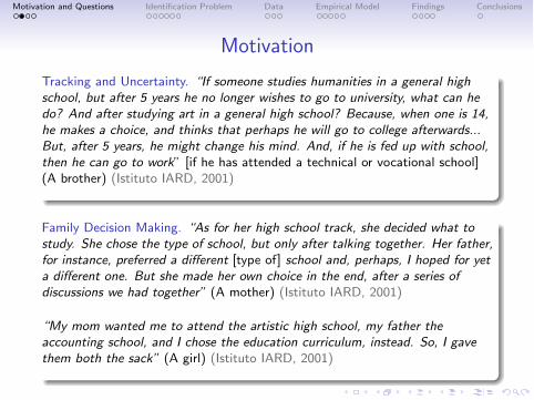
Tracking and Uncertainty. “If someone studies humanities in a general high

school, but after 5 years he no longer wishes to go to university, what can he

do? And after studying art in a general high school? Because, when one is 14,

he makes a choice, and thinks that perhaps he will go to college afterwards...

But, after 5 years, he might change his mind. And, if he is fed up with school,

then he can go to work” [if he has attended a technical or vocational school](A brother) (Istituto IARD, 2001)


Motivation

Tracking and Uncertainty. “If someone studies humanities in a general high

school, but after 5 years he no longer wishes to go to university, what can he

do? And after studying art in a general high school? Because, when one is 14,

he makes a choice, and thinks that perhaps he will go to college afterwards...

But, after 5 years, he might change his mind. And, if he is fed up with school,

then he can go to work” [if he has attended a technical or vocational school](A brother) (Istituto IARD, 2001)

Family Decision Making. “As for her high school track, she decided what to

study. She chose the type of school, but only after talking together. Her father,

for instance, preferred a different [type of] school and, perhaps, I hoped for yet

a different one. But she made her own choice in the end, after a series of

discussions we had together” (A mother) (Istituto IARD, 2001)

“My mom wanted me to attend the artistic high school, my father the

accounting school, and I chose the education curriculum, instead. So, I gave

them both the sack” (A girl) (Istituto IARD, 2001)


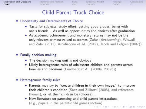
Child-Parent Track Choice• Uncertainty and Determinants of Choice

• Taste for subjects, study effort, getting good grades, being withone’s friends... As well as opportunities and choices after graduation

• As academic achievement and monetary returns may not be theonly relevant or most valued outcomes (Zafar (forthcoming), Wiswalland Zafar (2011), Arcidiacono et Al. (2012), Jacob and Lefgren (2007))

• Family decision making

• The decision making unit is not obvious• Likely heterogenous roles of adolescent children and parents across

families and decisions (Lundberg et Al. (2009a, 2009b))

• Heterogenous family rules

• Parents may try to “create children in their own image,” to improvetheir children’s condition (Saez and Zilibotti (2008), and referencestherein), or let their children be (choose)...

• New literature on parenting and child-parent interactions(e.g., papers in the parent-child games section)


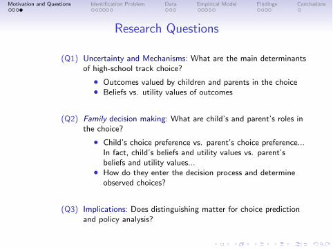
Research Questions

(Q1) Uncertainty and Mechanisms: What are the main determinantsof high-school track choice?

• Outcomes valued by children and parents in the choice• Beliefs vs. utility values of outcomes

(Q2) Family decision making: What are child’s and parent’s roles inthe choice?

• Child’s choice preference vs. parent’s choice preference...In fact, child’s beliefs and utility values vs. parent’sbeliefs and utility values...

• How do they enter the decision process and determineobserved choices?

(Q3) Implications: Does distinguishing matter for choice predictionand policy analysis?


General Identification Problem

• Typical data: Distribution of actual choices

• Problem: Multiple configurations of

• individual decision makers’ beliefs (about future outcomes),• individual decision makers’ utilities (of future outcomes),• group’s decision rule (decision participants’ “roles”)

are observationally equivalent...

⇒ General question: How to separate them? ⇐

• Context: Any real-life decision with uncertain outcomes and multipledecision makers, but no strategic interaction


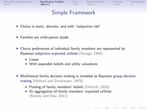
Simple Framework

• Choice is static, discrete, and with “subjective risk”

• Families are child-parent dyads

• Choice preferences of individual family members are represented byBayesian subjective expected utilities (Savage, 1954)

• Linear• With separable beliefs and utility valuations

• Multilateral family decision making is modeled as Bayesian group decisionmaking (Hylland and Zeckhauser, 1979)

• Pooling of family members’ beliefs (Dietrich, 2010)• Or aggregation of family members’ expected utilities

(Keeney and Nau, 2011)


A 2×2×2×2 Example

• 2 potential decision makers: i ∈ {child (c), parent (p)}

• 2 alternatives: j ∈ {Michelangelo (M), Galileo (G)}

• 2 binary outcomes:

1. outcome 1: child’s taste for subjects⇒ Pij1 = i ’s subjective probability that the child will enjoy

curriculum j ’s core subjects

2. outcome 2: flexibility in the future study vs. work choice⇒ Pij2 = i ’s subjective probability that the child will face

a wide range of education and work opportunitiesafter graduation from j

• 2 family decision rules:Γk ∈ {child unilaterally, child and parent jointly}


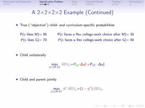
A 2×2×2×2 Example (Continued)

• True (“objective”) child- and curriculum-specific probabilities

P(c likes M)= 95 P(c faces a flex college-work choice after M)= 30

P(c likes G)= 70 P(c faces a flex college-work choice after G)= 90

• Child unilaterally

maxj∈{M,G}

SEUcj=Pcj1·∆uc1+Pcj2 ·∆u

c2

• Child and parent jointly

maxj∈{M,G}

φc ·SEUcj+(1− φc)·SEUpj


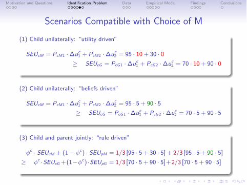
Scenarios Compatible with Choice of M

(1) Child unilaterally: “utility driven”

SEUcM = PcM1 ·∆uc1 + PcM2 ·∆u

c2 = 95 · 10 + 30 · 0

≥ SEUcG = PcG1 ·∆uc1 + PcG2 ·∆u

c2 = 70 · 10 + 90 · 0

(2) Child unilaterally: “beliefs driven”

SEUcM = PcM1 ·∆uc1 + PcM2 ·∆u

c2 = 95 · 5 + 90 · 5

≥ SEUcG = PcG1 ·∆uc1 + PcG2 ·∆u

c2 = 70 · 5 + 90 · 5

(3) Child and parent jointly: “rule driven”

φc · SEUcM + (1− φc) · SEUpM = 1/3 [95 · 5 + 30 · 5] + 2/3 [95 · 5 + 90 · 5]≥ φc ·SEUcG +(1−φc) ·SEUpG = 1/3 [70 · 5 + 90 · 5]+2/3 [70 · 5 + 90 · 5]


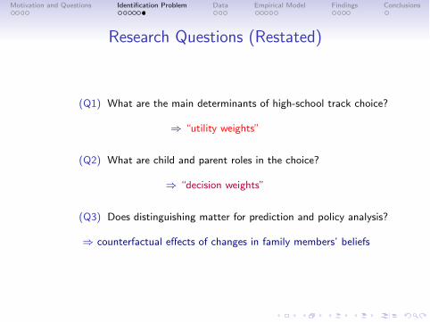
Research Questions (Restated)

(Q1) What are the main determinants of high-school track choice?

⇒ “utility weights”

(Q2) What are child and parent roles in the choice?

⇒ “decision weights”

(Q3) Does distinguishing matter for prediction and policy analysis?

⇒ counterfactual effects of changes in family members’ beliefs


A Survey in Northern Italy• Population: 9th graders enrolled for the first time in any public HS of the

Verona Municipality in Sept. 2007 and their parents (little over 4,000)

• Age of tracking 14• Retrospective survey during first week of high school• Choice-based sampling• 1 child questionnaire and 1 parent questionnaire

• Choice set: 10 main curricula offered in the municipality

• Tracks (general, technical, vocational) + curricula (core subjects)• Separate curricula (in different schools)• Open enrollment (and mostly public)

• Samples: 1,029 students (enrolled for the first time) and 608 parents

• Participating students (≈ 100%) filled their questionnaire in classduring 1 school hour, assisted by an instructor

• Parents took their questionnaire at home and returned through theschool within 7-10 days

• Institutional Details , Design Choices


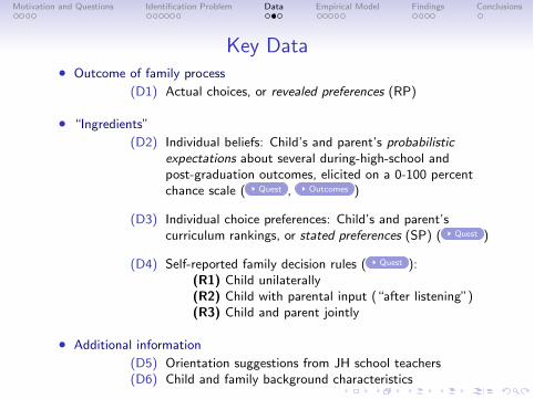
Key Data• Outcome of family process

(D1) Actual choices, or revealed preferences (RP)

• “Ingredients”

(D2) Individual beliefs: Child’s and parent’s probabilisticexpectations about several during-high-school andpost-graduation outcomes, elicited on a 0-100 percentchance scale ( Quest , Outcomes )

(D3) Individual choice preferences: Child’s and parent’scurriculum rankings, or stated preferences (SP) ( Quest )

(D4) Self-reported family decision rules ( Quest ):(R1) Child unilaterally(R2) Child with parental input (“after listening”)(R3) Child and parent jointly

• Additional information

(D5) Orientation suggestions from JH school teachers(D6) Child and family background characteristics


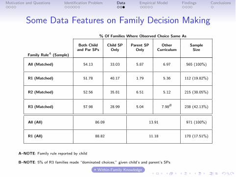
Some Data Features on Family Decision Making

% Of Families Where Observed Choice Same As

Both Child Child SP Parent SP Other Sampleand Par SPs Only Only Curriculum Size

Family RuleA (Sample)

All (Matched) 54.13 33.03 5.87 6.97 565 (100%)

R1 (Matched) 51.78 40.17 1.79 5.36 112 (19.82%)

R2 (Matched) 52.56 35.81 6.51 5.12 215 (38.05%)

R3 (Matched) 57.98 28.99 5.04 7.98B 238 (42.13%)

All (All) 86.09 13.91 971 (100%)

R1 (All) 88.82 11.18 170 (17.51%)

A–NOTE: Family rule reported by child

B–NOTE: 5% of R3 families made “dominated choices,” given child’s and parent’s SPs

Within-Family Knowledge


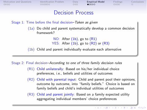
Decision Process

Stage 1: Time before the final decision–Taken as given

(1a) Do child and parent systematically develop a common decisionframework?

NO: After (1b), go to (R1)YES: After (1b), go to (R2) or (R3)

(1b) Child and parent individually evaluate each alternative

Stage 2: Final decision–According to one of three family decision rules

(R1) Child unilaterally: Based on his/her individual choicepreferences, i.e., beliefs and utilities of outcomes

(R2) Child with parental input: Child and parent pool their opinions,outcome by outcome, into “family beliefs.” Choice is based onfamily beliefs and child’s individual utilities of outcomes

(R3) Child and parent jointly: Based on a family expected utilityaggregating individual members’ choice preferences


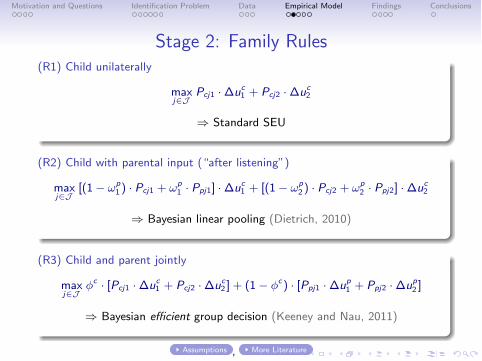
Stage 2: Family Rules(R1) Child unilaterally

maxj∈J

Pcj1 ·∆uc1 + Pcj2 ·∆u

c2

⇒ Standard SEU

(R2) Child with parental input (“after listening”)

maxj∈J

[(1− ωp1 ) · Pcj1 + ωp

1 · Ppj1] ·∆uc1 + [(1− ωp

2 ) · Pcj2 + ωp2 · Ppj2] ·∆u

c2

⇒ Bayesian linear pooling (Dietrich, 2010)

(R3) Child and parent jointly

maxj∈J

φc · [Pcj1 ·∆uc1 + Pcj2 ·∆u

c2 ] + (1− φc) · [Ppj1 ·∆u

p1 + Ppj2 ·∆u

p2 ]

⇒ Bayesian efficient group decision (Keeney and Nau, 2011)

Assumptions , More Literature


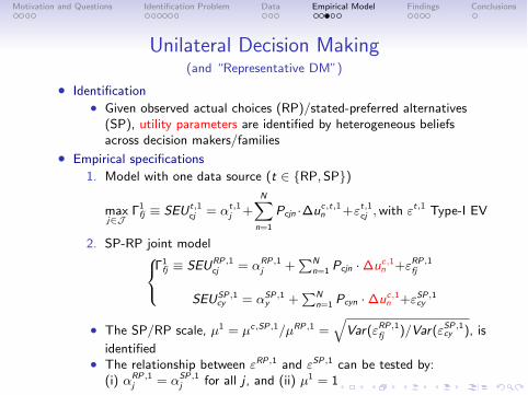
Unilateral Decision Making(and “Representative DM”)

• Identification• Given observed actual choices (RP)/stated-preferred alternatives

(SP), utility parameters are identified by heterogeneous beliefsacross decision makers/families

• Empirical specifications1. Model with one data source (t ∈ {RP, SP})

maxj∈J

Γ1fj ≡ SEU

t,1cj = αt,1

j +N�

n=1

Pcjn ·∆uc,t,1n +εt,1cj ,with εt,1 Type-I EV

2. SP-RP joint model

Γ1fj ≡ SEU

RP,1cj = αRP,1

j +�N

n=1 Pcjn ·∆uc,1n +εRP,1

fj

SEUSP,1cy = αSP,1

y +�N

n=1 Pcyn ·∆uc,1n +εSP,1

cy

• The SP/RP scale, µ1 = µc,SP,1/µRP,1 =�

Var(εRP,1fj )/Var(εSP,1

cy ), is

identified• The relationship between εRP,1 and εSP,1 can be tested by:

(i) αRP,1j = αSP,1

j for all j , and (ii) µ1 = 1


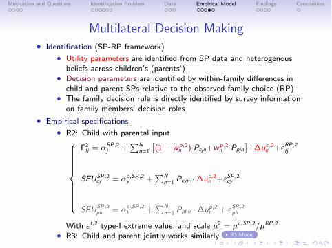
Multilateral Decision Making• Identification (SP-RP framework)

• Utility parameters are identified from SP data and heterogenousbeliefs across children’s (parents’)

• Decision parameters are identified by within-family differences inchild and parent SPs relative to the observed family choice (RP)

• The family decision rule is directly identified by survey informationon family members’ decision roles

• Empirical specifications

• R2: Child with parental input

Γ2fj = αRP,2

j +�N

n=1

�(1− w

p,2n )·Pcjn+w

p,2n ·Ppjn

�·∆u

c,2n +εRP,2

fj

SEUSP,2cy = αc,SP,2

y +�N


cy

SEUSP,2ph = αp,SP,2

h +�N

n=1 Pphn ·∆up,2n + εSP,2

ph

With εt,2 type-I extreme value, and scale µ2 = µc,SP,2/µRP,2

• R3: Child and parent jointly works similarly R3 Model


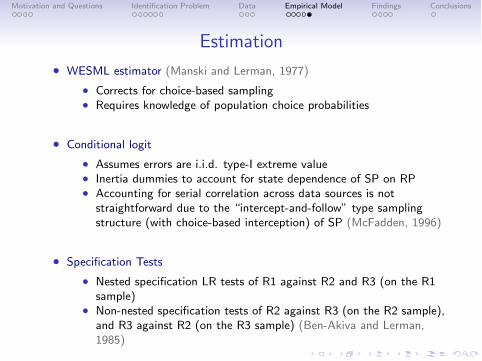
Estimation

• WESML estimator (Manski and Lerman, 1977)

• Corrects for choice-based sampling• Requires knowledge of population choice probabilities

• Conditional logit

• Assumes errors are i.i.d. type-I extreme value• Inertia dummies to account for state dependence of SP on RP• Accounting for serial correlation across data sources is not

straightforward due to the “intercept-and-follow” type samplingstructure (with choice-based interception) of SP (McFadden, 1996)

• Specification Tests

• Nested specification LR tests of R1 against R2 and R3 (on the R1sample)

• Non-nested specification tests of R2 against R3 (on the R2 sample),and R3 against R2 (on the R3 sample) (Ben-Akiva and Lerman,1985)


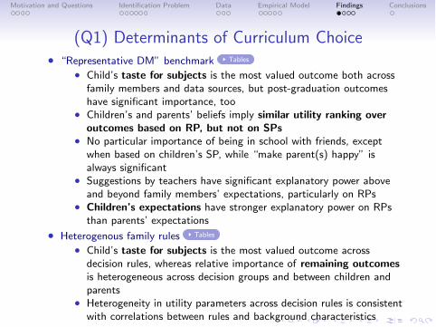
(Q1) Determinants of Curriculum Choice• “Representative DM” benchmark Tables

• Child’s taste for subjects is the most valued outcome both acrossfamily members and data sources, but post-graduation outcomeshave significant importance, too

• Children’s and parents’ beliefs imply similar utility ranking overoutcomes based on RP, but not on SPs

• No particular importance of being in school with friends, exceptwhen based on children’s SP, while “make parent(s) happy” isalways significant

• Suggestions by teachers have significant explanatory power aboveand beyond family members’ expectations, particularly on RPs

• Children’s expectations have stronger explanatory power on RPsthan parents’ expectations

• Heterogenous family rules Tables

• Child’s taste for subjects is the most valued outcome acrossdecision rules, whereas relative importance of remaining outcomesis heterogeneous across decision groups and between children andparents

• Heterogeneity in utility parameters across decision rules is consistentwith correlations between rules and background characteristics


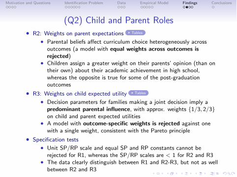
(Q2) Child and Parent Roles• R2: Weights on parent expectations Tables

• Parental beliefs affect curriculum choice heterogeneously acrossoutcomes (a model with equal weights across outcomes isrejected)

• Children assign a greater weight on their parents’ opinion (than ontheir own) about their academic achievement in high school,whereas the opposite is true for some of the post-graduationoutcomes

• R3: Weights on child expected utility Tables

• Decision parameters for families making a joint decision imply apredominant parental influence, with approx. weights {1/3, 2/3}on child and parent expected utilities

• A model with outcome-specific weights is rejected against onewith a single weight, consistent with the Pareto principle

• Specification tests

• Unit SP/RP scale and equal SP and RP constants cannot berejected for R1, whereas the SP/RP scales are < 1 for R2 and R3

• The data clearly distinguish between R1 and R2-R3, but not as wellbetween R2 and R3


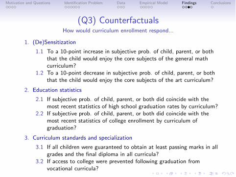
(Q3) CounterfactualsHow would curriculum enrollment respond...

1. (De)Sensitization

1.1 To a 10-point increase in subjective prob. of child, parent, or boththat the child would enjoy the core subjects of the general mathcurriculum?

1.2 To a 10-point decrease in subjective prob. of child, parent, or boththat the child would enjoy the core subjects of the art curriculum?

2. Education statistics

2.1 If subjective prob. of child, parent, or both did coincide with themost recent statistics of high school graduation rates by curriculum?

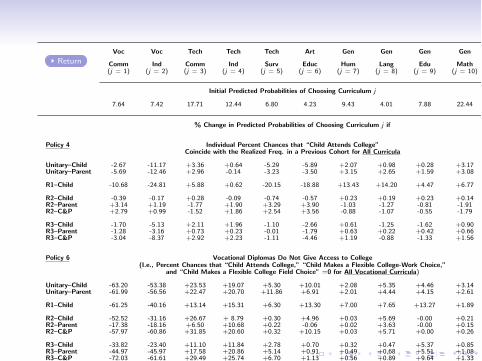
2.2 If subjective prob. of child, parent, or both did coincide with themost recent statistics of college enrollment by curriculum ofgraduation?

3. Curriculum standards and specialization

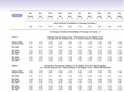
3.1 If all children were guaranteed to obtain at least passing marks in allgrades and the final diploma in all curricula?

3.2 If access to college were prevented following graduation fromvocational curricula?


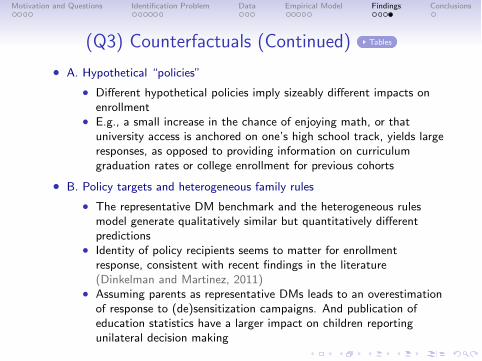
(Q3) Counterfactuals (Continued) Tables

• A. Hypothetical “policies”

• Different hypothetical policies imply sizeably different impacts onenrollment

• E.g., a small increase in the chance of enjoying math, or thatuniversity access is anchored on one’s high school track, yields largeresponses, as opposed to providing information on curriculumgraduation rates or college enrollment for previous cohorts

• B. Policy targets and heterogeneous family rules

• The representative DM benchmark and the heterogeneous rulesmodel generate qualitatively similar but quantitatively differentpredictions

• Identity of policy recipients seems to matter for enrollmentresponse, consistent with recent findings in the literature(Dinkelman and Martinez, 2011)

• Assuming parents as representative DMs leads to an overestimationof response to (de)sensitization campaigns. And publication ofeducation statistics have a larger impact on children reportingunilateral decision making


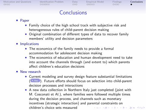
Conclusions• Paper

• Family choice of the high school track with subjective risk andheterogeneous rules of child-parent decision making

• Original combination of different types of data to recover familymembers’ utility and decision parameters

• Implications• The economics of the family needs to provide a formal

accommodation for adolescent decision making• The economics of education and human development need to take

into account the channels through (and extent to) which parentsaffect children’s education decisions

• New research• Current modeling and survey design feature substantial limitations

( Ass. ). Future efforts should focus on selection into child-parentdecision processes and interactions

• A new data collection in Northern Italy just completed (joint withM. Cosconati et Al.), where families were followed multiple timesduring the decision process, and channels such as monetaryincentives (strategic interaction) and parental constraints onchildren’s choice sets measured

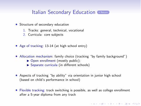
Italian Secondary Education Return

• Structure of secondary education

1. Tracks: general, technical, vocational2. Curricula: core subjects

• Age of tracking: 13-14 (at high school entry)

• Allocation mechanism: family choice (tracking “by family background”)� Open enrollment (mostly public);� Separate curricula (in different schools)

• Aspects of tracking “by ability” via orientation in junior high school(based on child’s performance in school)

• Flexible tracking: track switching is possible, as well as college enrollmentafter a 5-year diploma from any track

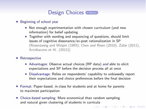
Design Choices Return

• Beginning of school year

• Not enough experimentation with chosen curriculum (and newinformation) for belief updating

• Together with wording and sequencing of questions, should limitissues of cognitive dissonance/ex-post rationalization in SP(Rosenzweig and Wolpin (1993); Chen and Risen (2010), Zafar (2011),Arcidiacono et Al. (2012))

• Retrospective

• Advantages: Observe actual choices (RP data) and able to elicitexpectations and SP before the decision process all at once

• Disadvantage: Relies on respondents’ capability to unbiasedly reporttheir expectations and choice preferences before the final decision

• Format: Paper-based, in-class for students and at home for parentsto maximize participation

• Choice-based sampling: More economical than random samplingand natural given clustering of students in curricula

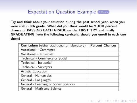
Expectation Question Example Return

Try and think about your situation during the past school year, when youwere still in 8th grade. What did you think would be YOUR percentchance of PASSING EACH GRADE on the FIRST TRY and finallyGRADUATING from the following curricula, should you enroll in each onethem?

Curriculum (either traditional or laboratory) Percent ChancesVocational - CommerceVocational - IndustrialTechnical - Commerce or SocialTechnical - IndustrialTechnical - SurveyorsArtistic EducationGeneral - HumanitiesGeneral - LanguagesGeneral - Learning or Social SciencesGeneral - Math and Science

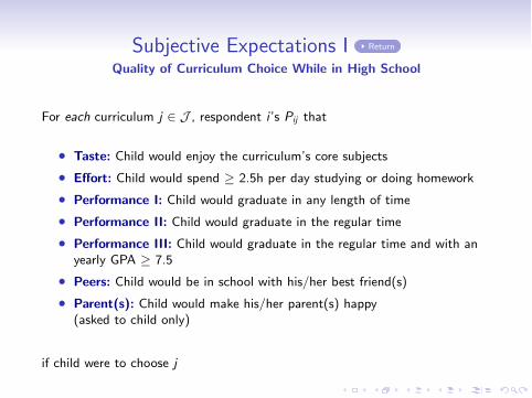
Subjective Expectations I Return

Quality of Curriculum Choice While in High School

For each curriculum j ∈ J , respondent i ’s Pij that

• Taste: Child would enjoy the curriculum’s core subjects

• Effort: Child would spend ≥ 2.5h per day studying or doing homework

• Performance I: Child would graduate in any length of time

• Performance II: Child would graduate in the regular time

• Performance III: Child would graduate in the regular time and with anyearly GPA ≥ 7.5

• Peers: Child would be in school with his/her best friend(s)

• Parent(s): Child would make his/her parent(s) happy(asked to child only)

if child were to choose j

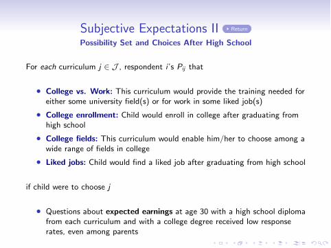
Subjective Expectations II Return

Possibility Set and Choices After High School

For each curriculum j ∈ J , respondent i ’s Pij that

• College vs. Work: This curriculum would provide the training needed foreither some university field(s) or for work in some liked job(s)

• College enrollment: Child would enroll in college after graduating fromhigh school

• College fields: This curriculum would enable him/her to choose among awide range of fields in college

• Liked jobs: Child would find a liked job after graduating from high school

if child were to choose j

• Questions about expected earnings at age 30 with a high school diplomafrom each curriculum and with a college degree received low responserates, even among parents

SP Question Return

Try and think about your situation during the past school year, when youwere still in 8th grade. Please, RANK the following curricula from the oneYOU like BEST to the one you like the LEAST for yourself, consideringthe criteria YOU considered important for choosing among them. Start byassigning 1 to YOUR FAVORITE curriculum, then proceed by incrementsof 1 till YOUR LEAST preferred one. The same number cannot beassigned to two different schools.

School (either traditional or laboratory) RankVocational - CommerceVocational - IndustrialTechnical - Commerce or SocialTechnical - IndustrialTechnical - SurveyorsArtistic EducationGeneral - HumanitiesGeneral - LanguagesGeneral - Learning or Social SciencesGeneral - Math and Science

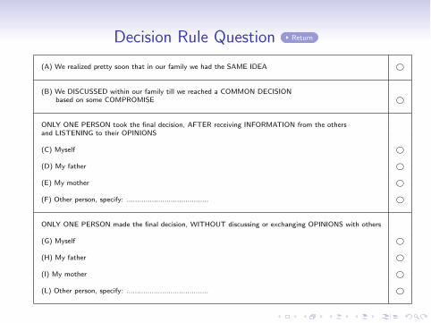
Decision Rule Question Return

(A) We realized pretty soon that in our family we had the SAME IDEA �

(B) We DISCUSSED within our family till we reached a COMMON DECISIONbased on some COMPROMISE �

ONLY ONE PERSON took the final decision, AFTER receiving INFORMATION from the othersand LISTENING to their OPINIONS

(C) Myself �

(D) My father �

(E) My mother �

(F) Other person, specify: ....................................... �

ONLY ONE PERSON made the final decision, WITHOUT discussing or exchanging OPINIONS with others

(G) Myself �

(H) My father �

(I) My mother �

(L) Other person, specify: ....................................... �

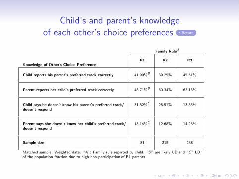
Child’s and parent’s knowledgeof each other’s choice preferences Return

Family RuleA

R1 R2 R3Knowledge of Other’s Choice Preference

Child reports his parent’s preferred track correctly 41.90%B 39.25% 45.61%

Parent reports her child’s preferred track correctly 48.71%B 60.34% 63.13%

Child says he doesn’t know his parent’s preferred track/ 31.82%C 28.51% 13.85%doesn’t respond

Parent says she doesn’t know her child’s preferred track/ 18.14%C 12.68% 14.23%doesn’t respond

Sample size 81 215 238

Matched sample. Weighted data. “A”: Family rule reported by child. “B” are likely UB and “C” LBof the population fraction due to high non-participation of R1 parents

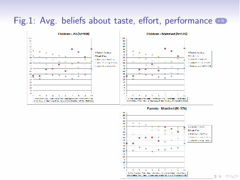
Fig.1: Avg. beliefs about taste, effort, performance R

Fig.2: Avg. beliefs in the vocational sample Return

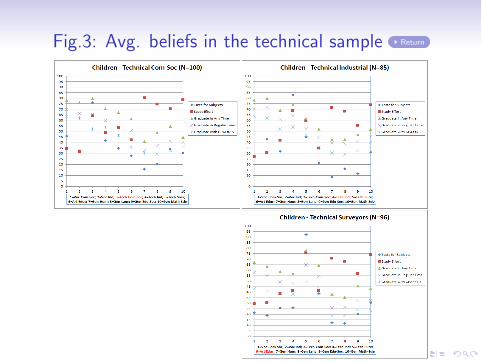
Fig.3: Avg. beliefs in the technical sample Return

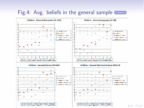
Fig.4: Avg. beliefs in the general sample Return

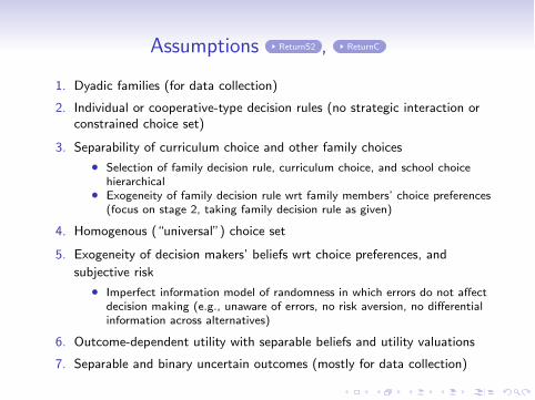
Assumptions ReturnS2 , ReturnC

1. Dyadic families (for data collection)

2. Individual or cooperative-type decision rules (no strategic interaction orconstrained choice set)

3. Separability of curriculum choice and other family choices

• Selection of family decision rule, curriculum choice, and school choicehierarchical

• Exogeneity of family decision rule wrt family members’ choice preferences(focus on stage 2, taking family decision rule as given)

4. Homogenous (“universal”) choice set

5. Exogeneity of decision makers’ beliefs wrt choice preferences, andsubjective risk

• Imperfect information model of randomness in which errors do not affectdecision making (e.g., unaware of errors, no risk aversion, no differentialinformation across alternatives)

6. Outcome-dependent utility with separable beliefs and utility valuations

7. Separable and binary uncertain outcomes (mostly for data collection)

Links with Literatures ReturnS2

• Cultural transmission (Saez-Marti and Zilibotti, 2008)

• Non-paternalistic features. Children and parents share the common goalof choosing the curriculum that suits the child best, accounting for bothnear- and later-future choice consequences (same objective function).With this very purpose, parents may try to affect children’s currentchoices (and, thus, future paths) via the channel of beliefs (R2), or bothbeliefs and utilities (R3)

• Paternalistic features. Parental role in the choice is based on parents’ ownbeliefs and utilities, which may differ from children’s (as in Bisin andVerdier (2001)’s “imperfect parental empathy”)

• Efficient group (household) behavior (Chiappori and Ekeland, 2009)

• I exploit information on family members’ decision roles to specifyheterogenous rules of child-parent decision making, as opposed to relyinguniquely on the assumption of Pareto efficiency

• I focus on the aspect of subjective risk/uncertainty characterizingcurriculum choice within a Bayesian framework, and do not addressimportant issues of consumption and saving under uncertainty, such asrisk sharing

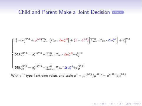
Child and Parent Make a Joint Decision Return

Γ3fj = αRP,3

j + φc,3�Nn=1

�Pcjn ·∆u

c,3n

�+ (1− φc,3)

��Nn=1 Ppjn ·∆u

p,3n

�+ εRP,3

fj

SEUSP,3cy = αc,SP,3

y +�N


cj

SEUSP,3ph = αc,SP,3

h +�N

n=1 Pphn ·∆up,3n +εSP,3

ph

With εt,3 type-I extreme value, and scale µ3 = µc,SP,3/µRP,3 = µp,SP,3/µRP,3

“Unitary Model” with RP DataAll Return

Child’s Expectations Parent’s Expectations

Outcomes (1) (2) (3) (4)

Like Subjects (1) 5.58∗∗∗ 5.75∗∗∗ (1) 8.14∗∗∗ 7.45∗∗∗

Avg. Daily Homework ≥ 2.5h 0.91∗∗ 0.58 0.97 0.89

Graduate in Regular Time (3) 1.59∗∗∗ 1.45∗∗∗ (3) 1.68∗∗ 1.68∗

In School with Friend(s) 0.11 −0.05 0.69 0.69

Flexible College-Work Choice 0.96∗∗∗ 1.21∗∗∗ 0.87∗ 0.99∗

Attend College 0.92∗∗ 1.22∗∗ 0.70 1.14

Flexible College Field Choice (2) 2.11∗∗∗ 2.19∗∗∗ (2) 2.64∗∗∗ 1.94∗∗∗

Liked Job after Graduation (5) 1.05∗∗∗ 0.98∗∗∗ (4) 1.18∗∗∗ 1.16∗∗

Parent Happy (3) 1.74∗∗∗ 1.74∗∗∗ − −

JHS Suggestion − (3) 1.49∗∗∗ − (2) 1.90∗∗∗

Constants Yes Yes Yes Yes

Log-likelihood -612.2726 -429.4309 -455.4374 -379.2716

Adjusted LR Index 0.726 0.773 0.651 0.686

Sample Size 998 857 588 550

∗∗∗ : significant at 1%, ∗∗ : significant at 5%, ∗ : significant at 10%

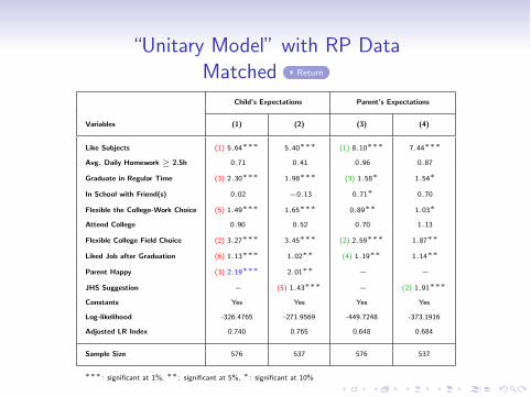
“Unitary Model” with RP DataMatched Return


Variables (1) (2) (3) (4)

Like Subjects (1) 5.64∗∗∗ 5.40∗∗∗ (1) 8.10∗∗∗ 7.44∗∗∗

Avg. Daily Homework ≥ 2.5h 0.71 0.41 0.96 0.87

Graduate in Regular Time (3) 2.30∗∗∗ 1.98∗∗∗ (3) 1.58∗ 1.54∗

In School with Friend(s) 0.02 −0.13 0.71∗ 0.70

Flexible the College-Work Choice (5) 1.49∗∗∗ 1.65∗∗∗ 0.89∗∗ 1.03∗

Attend College 0.90 0.52 0.70 1.13

Flexible College Field Choice (2) 3.27∗∗∗ 3.45∗∗∗ (2) 2.59∗∗∗ 1.87∗∗

Liked Job after Graduation (6) 1.13∗∗∗ 1.02∗∗ (4) 1.19∗∗ 1.14∗∗

Parent Happy (3) 2.19∗∗∗ 2.01∗∗ − −

JHS Suggestion − (5) 1.43∗∗∗ − (2) 1.91∗∗∗


Log-likelihood -326.4765 -271.9569 -449.7248 -373.1916


Sample Size 576 537 576 537


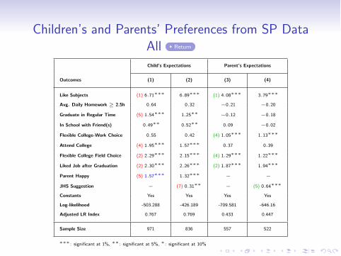
Children’s and Parents’ Preferences from SP DataAll Return


Outcomes (1) (2) (3) (4)

Like Subjects (1) 6.71∗∗∗ 6.89∗∗∗ (1) 4.08∗∗∗ 3.79∗∗∗

Avg. Daily Homework ≥ 2.5h 0.64 0.32 −0.21 −0.20

Graduate in Regular Time (5) 1.54∗∗∗ 1.25∗∗ −0.12 −0.18

In School with Friend(s) 0.49∗∗ 0.52∗∗ 0.09 −0.02

Flexible College-Work Choice 0.55 0.42 (4) 1.05∗∗∗ 1.13∗∗∗

Attend College (4) 1.95∗∗∗ 1.57∗∗∗ 0.37 0.39

Flexible College Field Choice (2) 2.29∗∗∗ 2.15∗∗∗ (4) 1.29∗∗∗ 1.22∗∗∗

Liked Job after Graduation (2) 2.30∗∗∗ 2.26∗∗∗ (2) 1.87∗∗∗ 1.94∗∗∗

Parent Happy (5) 1.57∗∗∗ 1.32∗∗∗ − −

JHS Suggestion − (7) 0.31∗∗ − (5) 0.64∗∗∗


Log-likelihood -503.288 -426.189 -709.581 -646.16


Sample Size 971 836 557 522


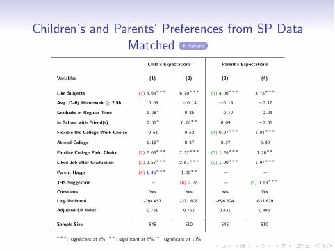
Children’s and Parents’ Preferences from SP DataMatched Return


Variables (1) (2) (3) (4)

Like Subjects (1) 6.64∗∗∗ 6.70∗∗∗ (1) 4.06∗∗∗ 3.78∗∗∗

Avg. Daily Homework ≥ 2.5h 0.08 −0.14 −0.19 −0.17

Graduate in Regular Time 1.08∗ 0.85 −0.19 −0.24

In School with Friend(s) 0.61∗ 0.64∗∗ 0.09 −0.01

Flexible the College-Work Choice 0.51 0.52 (4) 0.97∗∗∗ 1.04∗∗∗

Attend College 1.16∗ 0.87 0.37 0.39

Flexible College Field Choice (2) 2.63∗∗∗ 2.37∗∗∗ (3) 1.26∗∗∗ 1.20∗∗

Liked Job after Graduation (2) 2.57∗∗∗ 2.61∗∗∗ (2) 1.90∗∗∗ 1.97∗∗∗

Parent Happy (4) 1.46∗∗∗ 1.38∗∗ − −

JHS Suggestion − (6) 0.27 − (5) 0.63∗∗∗


Log-likelihood -294.457 -271.808 -696.524 -633.629


Sample Size 545 510 545 510


“Child Chooses Unilaterally” Return

RP Model SP Model SP-RP Model

Variables (1) (2) (3) (4) (5) (6)

Like Subjects (1) 6.46∗∗∗ 6.40∗∗∗ (1) 5.65∗∗∗ 5.69∗∗∗ (1) 6.55∗∗∗ 6.57∗∗∗

Daily Homework ≥ 2.5h −1.20 −2.80∗∗∗ −0.06 −0.96 −0.73∗∗ −2.06∗

Graduate in Regular Time (4) 2.91∗∗∗ 2.60∗∗ 1.91∗ 1.70 (4) 2.59∗∗∗ 2.21∗∗

In School with Friend(s) 0.48 0.53 0.31 0.24 0.42 0.48

Flex. College-Work Choice 1.55∗ 2.89∗∗∗ 0.43 0.92 1.14 2.08∗∗

Attend College (2) 3.95∗∗∗ 5.24∗∗∗ (3) 2.53∗∗ 2.37∗∗ (2) 3.49∗∗∗ 4.02∗∗

Flex. Coll. Field Choice RP 0.32 −1.22∗∗∗ − − 0.42 −1.08

Flex. Coll. Field Choice SP − − (3) 2.41∗∗ 1.46 (4) 2.87∗∗ 1.65

Liked Job after Grad. RP 0.88 1.47∗ − − 0.87 1.23

Liked after Grad. Job SP − − (2) 3.13∗∗∗ 3.55∗∗∗ (2) 3.55∗∗∗ 4.14∗∗∗

Parent Happy (3) 3.23∗∗∗ 3.52∗∗∗ (3) 2.77∗∗ 3.38∗∗ (2) 3.22∗∗∗ 3.65∗∗∗

JHS Suggestion RP − (7) 2.32∗∗∗ − − − (5) 2.26∗∗∗

JHS Suggestion SP − − − (5) 1.14∗∗∗ − (7) 1.50∗∗

SP/RP Scale − − − − 0.845∗∗∗ 0.813∗∗∗

Constants Yes Yes Yes Yes Yes Yes

Log-likelihood -85.159 -56.210 -88.230 -69.626 -174.317 -127.823

Adjusted LR Index 0.736 0.773 0.729 0.733 0.739 0.759

Sample Size 170 144 170 144 170 144

∗∗∗ : significant at 1%, ∗∗ :significant at 5%, ∗ : significant at 10%

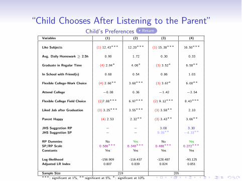
“Child Chooses After Listening to the Parent”Child’s Preferences Return

Variables (1) (2) (3) (4)

Like Subjects (1) 12.43∗∗∗ 12.20∗∗∗ (1) 15.38∗∗∗ 16.50∗∗∗


Graduate in Regular Time (4) 2.94∗ 4.06∗ (3) 3.52∗ 6.58∗∗

In School with Friend(s) 0.68 0.54 0.86 1.03

Flexible College-Work Choice (4) 2.66∗∗ 3.60∗∗∗ (3) 3.67∗ 6.00∗∗

Attend College −0.08 0.36 −1.42 −2.54

Flexible College Field Choice (2)7.88∗∗∗ 6.97∗∗∗ (2) 9.12∗∗∗ 8.43∗∗∗

Liked Job after Graduation (3) 3.25∗∗∗ 3.55∗∗∗ (3) 3.58∗∗ 2.10

Parent Happy (4) 2.53 2.32∗∗ (3) 3.43∗∗ 3.66∗∗

JHS Suggestion RP − − 3.08 3.30

JHS Suggestion SP − − 0.35∗∗ −4.33∗∗

RP Dummies No Yes No Yes

SP/RP Scale 0.586∗∗∗ 0.348∗∗∗ 0.488∗∗∗ 0.272∗∗∗Constants Yes Yes Yes Yes

Log-likelihood -156.909 -116.437 -128.487 -93.125


Sample Size 219 205∗∗∗ : significant at 1%, ∗∗ :significant at 5%, ∗ : significant at 10%

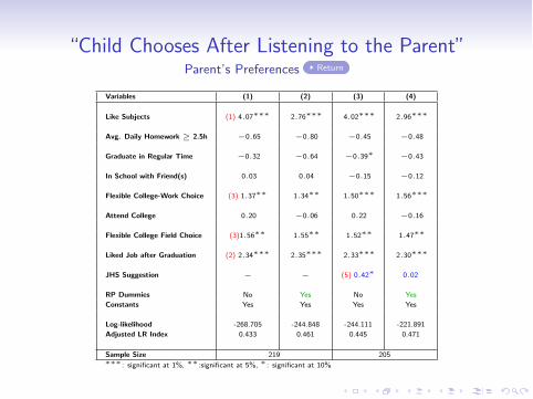
“Child Chooses After Listening to the Parent”Parent’s Preferences Return

Variables (1) (2) (3) (4)

Like Subjects (1) 4.07∗∗∗ 2.76∗∗∗ 4.02∗∗∗ 2.96∗∗∗

Avg. Daily Homework ≥ 2.5h −0.65 −0.80 −0.45 −0.48

Graduate in Regular Time −0.32 −0.64 −0.39∗ −0.43

In School with Friend(s) 0.03 0.04 −0.15 −0.12

Flexible College-Work Choice (3) 1.37∗∗ 1.34∗∗ 1.50∗∗∗ 1.56∗∗∗

Attend College 0.20 −0.06 0.22 −0.16

Flexible College Field Choice (3)1.56∗∗ 1.55∗∗ 1.52∗∗ 1.47∗∗

Liked Job after Graduation (2) 2.34∗∗∗ 2.35∗∗∗ 2.33∗∗∗ 2.30∗∗∗

JHS Suggestion − − (5) 0.42∗ 0.02

RP Dummies No Yes No Yes


Log-likelihood -268.705 -244.848 -244.111 -221.891


Sample Size 219 205∗∗∗ : significant at 1%, ∗∗ :significant at 5%, ∗ : significant at 10%

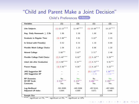
“Child and Parent Make a Joint Decision”Child’s Preferences Return

Variables (1) (2) (1) (2)

Like Subjects (1) 12.13∗∗∗ 11.49∗∗∗ (1) 13.58∗∗∗ 13.23∗∗∗


Graduate in Regular Time (3) 3.88∗∗ 3.81 3.10∗ 2.33

In School with Friend(s) 0.52 0.31 1.10 0.69

Flexible Work-College Choice 1.04 1.15 0.86 1.20

Attend College 2.88∗∗ 2.67∗ 2.71∗ 2.48

Flexible College Field Choice (2) 5.49∗∗∗ 6.02∗ (2) 5.18∗∗ 5.29∗∗

Liked Job after Graduation (3) 3.98∗∗∗ 4.15∗∗ (2) 4.72∗∗ 5.91∗∗

Parent Happy (3) 3.56∗∗ 4.05∗ (2) 4.18∗∗ 5.22∗∗

JHS Suggestion RP − − (5) 1.13∗∗∗ 1.15∗∗∗JHS Suggestion SP − − −0.04 −2.61∗∗

RP Dummies No Yes No YesSP/RP Scale 0.524∗∗∗ 0.329∗∗ 0.486∗∗∗ 0.280∗∗∗Constants Yes Yes Yes Yes

Log-likelihood -501.9089 -445.5068 -457.8141 -407.4601Adjusted LR Index 0.664 0.689 0.671 0.690

Sample Size 238 223∗∗∗ : significant at 1%, ∗∗ : significant at 5%, ∗ : significant at 10%

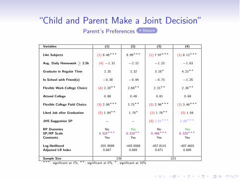
“Child and Parent Make a Joint Decision”Parent’s Preferences Return

Variables (1) (2) (3) (4)

Like Subjects (1) 8.46∗∗∗ 8.99∗∗∗ (1) 7.97∗∗∗ (1) 8.12∗∗∗

Avg. Daily Homework ≥ 2.5h (4) −1.31 −2.12 −1.23 −1.63

Graduate in Regular Time 2.35 3.32 3.18∗ 4.23∗∗

In School with Friend(s) −0.38 −0.94 −0.73 −1.25

Flexible Work-College Choice (4) 2.20∗∗ 2.68∗∗ 2.15∗∗ 2.36∗∗

Attend College 0.88 0.48 0.81 0.69

Flexible College Field Choice (3) 2.96∗∗∗ 3.75∗∗ (3) 2.96∗∗∗ (3) 3.46∗∗∗

Liked Job after Graduation (2) 1.84∗∗ 1.70∗ (2) 1.78∗∗ (2) 1.58

JHS Suggestion SP − − (3) 2.01∗∗∗ 2.06∗∗∗

RP Dummies No Yes No YesSP/RP Scale 0.524∗∗∗ 0.329∗∗ 0.486∗∗∗ 0.329∗∗∗Constants Yes Yes Yes Yes


Sample Size 238 223∗∗∗ : significant at 1%, ∗∗ : significant at 5%, ∗ : significant at 10%

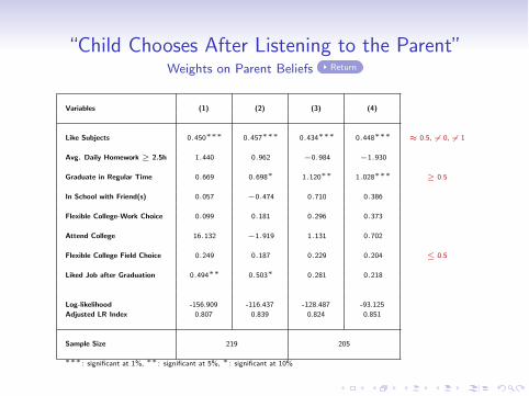
“Child Chooses After Listening to the Parent”Weights on Parent Beliefs Return

Variables (1) (2) (3) (4)

Like Subjects 0.450∗∗∗ 0.457∗∗∗ 0.434∗∗∗ 0.448∗∗∗ ≈ 0.5, �= 0, �= 1

Avg. Daily Homework ≥ 2.5h 1.440 0.962 −0.984 −1.930

Graduate in Regular Time 0.669 0.698∗ 1.120∗∗ 1.028∗∗∗ ≥ 0.5

In School with Friend(s) 0.057 −0.474 0.710 0.386

Flexible College-Work Choice 0.099 0.181 0.296 0.373

Attend College 16.132 −1.919 1.131 0.702

Flexible College Field Choice 0.249 0.187 0.229 0.204 ≤ 0.5

Liked Job after Graduation 0.494∗∗ 0.503∗ 0.281 0.218

Log-likelihood -156.909 -116.437 -128.487 -93.125


Sample Size 219 205


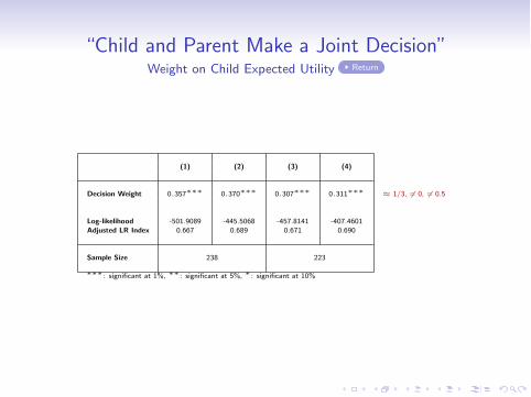
“Child and Parent Make a Joint Decision”Weight on Child Expected Utility Return

(1) (2) (3) (4)

Decision Weight 0.357∗∗∗ 0.370∗∗∗ 0.307∗∗∗ 0.311∗∗∗ ≈ 1/3, �= 0, �= 0.5


Sample Size 238 223


Voc Voc Tech Tech Tech Art Gen Gen Gen Gen

Return Comm Ind Comm Ind Surv Educ Hum Lan Edu Math(j = 1) (j = 2) (j = 3) (j = 4) (j = 5) (j = 6) (j = 7) (j = 8) (j = 9) (j = 10)

Initial Predicted Probabilities of Choosing Curriculum j

7.64 7.42 17.71 12.44 6.80 4.23 9.43 4.01 7.88 22.44

% Change in Predicted Probabilities of Choosing Curriculum j Following

Policy 1 An Increase in Percent Chances that “Child Likes the Subjects” in General Math-Scie by 10

Unitary–Child -1.29 -1.73 -1.38 -2.27 -3.97 -1.99 -8.40 -7.61 -3.78 +11.16Unitary–Parent -2.53 -3.05 -3.50 -5.04 -4.63 -3.47 -11.58 -12.36 -6.76 +18.93

R1–Child -1.28 -0.84 -0.26 -1.76 -3.51 -2.01 -4.78 -1.58 -4.02 +7.04

R2–Child -0.30 -0.14 -1.09 -3.64 -1.42 -0.20 -5.44 -3.93 -0.71 +6.74R2–Parent -0.23 -0.10 -0.83 -2.71 -1.02 -0.18 -4.17 -2.90 -0.50 +5.06R2–C&P -0.50 -0.24 -2.02 -6.95 -3.16 -0.28 -9.63 -7.99 -1.58 +12.73

R3–Child -0.73 -0.54 -0.40 -0.76 -1.12 -2.93 -4.94 -7.33 -2.75 +6.41R3–Parent -0.94 -0.73 -0.55 -0.98 -1.43 -3.85 -6.61 -9.71 -3.67 +8.50R3–C&P -1.49 -1.34 -1.00 -1.68 -2.29 -6.62 -11.89 -17.20 -6.66 +15.03

Policy 2 A Decrease in Percent Chances that “Child Likes the Subjects” in Artistic Educ by 10

Unitary–Child +0.86 +0.41 +0.45 +0.21 +1.53 -13.77 +0.46 +1.20 +1.50 +0.29Unitary–Parent +0.88 +0.72 +0.57 +0.59 +1.79 -18.91 +1.17 +2.02 +0.92 +0.54

R1–Child +0.48 +0.83 +0.17 +0.14 +0.95 -15.33 +0.93 +2.61 +2.24 +0.31

R2–Child +0.01 +0.06 +0.06 -0.02 +0.13 -6.20 +1.80 +0.23 +0.80 -0.01R2–Parent +0.00 +0.06 +0.06 -0.03 +0.11 -4.70 +1.33 +0.16 +0.64 -0.01R2–C&P +0.01 +0.07 +0.07 -0.02 +0.19 -11.43 +3.58 +0.57 +1.21 -0.01

R3–Child +0.12 +0.11 +0.12 +0.01 +0.72 -6.13 +0.31 +0.31 +0.18 +0.52R3–Parent +0.17 +0.12 +0.13 +0.02 +0.94 -7.86 +0.39 +0.43 +0.21 +0.67R3–C&P +0.37 +0.20 +0.20 +0.06 +1.51 -13.53 +0.66 +0.86 +0.40 +1.14


Return Comm Ind Comm Ind Surv Educ Hum Lang Edu Math(j = 1) (j = 2) (j = 3) (j = 4) (j = 5) (j = 6) (j = 7) (j = 8) (j = 9) (j = 10)


7.64 7.42 17.71 12.44 6.80 4.23 9.43 4.01 7.88 22.44

% Change in Predicted Probabilities of Choosing Curriculum j if

Policy 3 Individual Percent Chances that “Child Graduates in the Regular Time”Coincide with the Realized Freq. in a Previous Cohort for All Curricula

Unitary–Child -2.15 -3.42 +0.35 -1.72 -4.09 -7.37 +4.03 +0.43 -0.65 +3.63Unitary–Parent -4.47 -5.23 +0.15 -3.83 -0.67 -5.11 +5.94 +2.62 -1.56 +4.00

R1–Child -0.94 -6.32 +0.34 -4.09 -3.51 -9.81 +3.70 +4.12 -1.23 +5.46

R2–Child -1.73 -0.17 -0.50 +0.38 +0.16 +0.41 -0.85 +0.12 +0.27 -0.23R2–Parent -4.30 -0.12 +1.06 -2.94 -2.23 -5.10 +3.93 +4.12 +0.64 +1.32R2–C&P -3.07 -0.32 +0.73 -2.39 -2.05 -4.32 +2.86 +4.30 +1.07 +0.99

R3–Child -2.48 -2.88 +0.22 +1.47 -1.89 -3.39 +1.28 -2.63 +0.79 +1.68R3–Parent -5.74 -4.57 +0.09 +0.75 -1.19 -3.64 +2.86 -0.70 +1.80 +2.31R3–C&P -7.53 -6.94 +0.10 +1.87 -2.89 -7.21 +4.15 -3.14 +2.38 +3.96

Policy 5 Everybody Is Guaranteed a Diploma in the Regular Time from Any Curriculum(I.e., Percent Chances that “Child Graduates in the Regular Time”=100 for All Curricula)

Unitary–Child -2.35 -2.29 +0.57 +0.53 -2.63 -6.35 +1.62 +0.36 -0.59 +2.27Unitary–Parent -4.38 -3.78 +0.61 +0.63 +0.77 -3.66 +2.07 +2.30 -1.63 +1.66

R1–Child -0.47 -5.11 -0.11 -0.57 -2.28 -7.40 +0.20 +2.20 -0.92 +4.19

R2–Child +1.68 -0.15 -0.53 +0.08 +0.02 +0.19 -0.54 +0.08 +0.27 -0.07R2–Parent -4.25 -0.30 +1.42 +0.35 -1.01 -2.33 +0.74 +5.05 +0.88 -0.55R2–C&P -3.03 -0.50 +1.03 +0.47 -0.98 -1.94 +0.10 +5.13 +1.23 -0.60

R3–Child -2.60 -2.65 +0.32 +2.43 -1.64 -2.52 +0.22 -2.12 +0.78 +1.15R3–Parent -6.00 -4.00 +0.35 +2.92 -0.56 -1.94 +0.54 +0.32 +1.74 +1.12R3–C&P -7.99 -6.16 +0.44 +5.06 -2.08 -4.47 +0.67 -1.52 +2.40 +2.23


Return Comm Ind Comm Ind Surv Educ Hum Lang Edu Math(j = 1) (j = 2) (j = 3) (j = 4) (j = 5) (j = 6) (j = 7) (j = 8) (j = 9) (j = 10)


7.64 7.42 17.71 12.44 6.80 4.23 9.43 4.01 7.88 22.44

% Change in Predicted Probabilities of Choosing Curriculum j if

Policy 4 Individual Percent Chances that “Child Attends College”Coincide with the Realized Freq. in a Previous Cohort for All Curricula

Unitary–Child -2.67 -11.17 +3.36 +0.64 -5.29 -5.89 +2.07 +0.98 +0.28 +3.17Unitary–Parent -5.69 -12.46 +2.96 -0.14 -3.23 -3.50 +3.15 +2.65 +1.59 +3.08

R1–Child -10.68 -24.81 +5.88 +0.62 -20.15 -18.88 +13.43 +14.20 +4.47 +6.77

R2–Child -0.39 -0.17 +0.28 -0.09 -0.74 -0.57 +0.23 +0.19 +0.23 +0.14R2–Parent +3.14 +1.19 -1.77 +1.90 +3.29 +3.90 -1.03 -1.27 -0.81 -1.91R2–C&P +2.79 +0.99 -1.52 +1.86 +2.54 +3.56 -0.88 -1.07 -0.55 -1.79

R3–Child -1.70 -5.13 +2.11 +1.96 -1.10 -2.66 +0.61 -1.25 -1.62 +0.90R3–Parent -1.28 -3.16 +0.73 +0.23 -0.01 -1.79 +0.63 +0.22 +0.42 +0.66R3–C&P -3.04 -8.37 +2.92 +2.23 -1.11 -4.46 +1.19 -0.88 -1.33 +1.56

Policy 6 Vocational Diplomas Do Not Give Access to College(I.e., Percent Chances that “Child Attends College,” “Child Makes a Flexible College-Work Choice,”

and “Child Makes a Flexible College Field Choice” =0 for All Vocational Curricula)

Unitary–Child -63.20 -53.38 +23.53 +19.07 +5.30 +10.01 +2.08 +5.35 +4.46 +3.14Unitary–Parent -61.99 -56.56 +22.47 +20.70 +11.86 +6.91 +2.01 +4.44 +4.15 +2.61

R1–Child -61.25 -40.16 +13.14 +15.31 +6.30 +13.30 +7.00 +7.65 +13.27 +1.89

R2–Child -52.52 -31.16 +26.67 + 8.79 +0.30 +4.96 +0.03 +5.69 -0.00 +0.21R2–Parent -17.38 -18.16 +6.50 +10.68 +0.22 -0.06 +0.02 +3.63 -0.00 +0.15R2–C&P -57.97 -60.86 +31.85 +20.60 +0.32 +10.15 +0.03 +5.71 +0.00 +0.26

R3–Child -33.82 -23.40 +11.10 +11.84 +2.78 +0.70 +0.32 +0.47 +5.37 +0.85R3–Parent -44.97 -45.97 +17.58 +20.86 +5.14 +0.91 +0.49 +0.68 +5.51 +1.08R3–C&P -72.03 -61.61 +29.49 +25.74 +6.70 +1.13 +0.56 +0.89 +9.64 +1.33

Group Decision Making with Uncertain Outcomes: … and Questions Identiﬁcation Problem Data...

Documents

Transcript of Group Decision Making with Uncertain Outcomes: … and Questions Identiﬁcation Problem Data...