GROUNDWATER RECHARGE AND DISCHARGE IN A SALINE, URBAN CATCHMENT;

WAGGA WAGGA, NEW SOUTH WALES

P.G. Cook1, M. Stauffacher1, R. Therrien2, T. Halihan3, P. Richardson1, R.M. Williams4 and A. Bradford1

1 CSIRO Land and Water 2 Laval University, Canada

3 University of Texas 4 NSW Department of Land and Water Conservation

2

3

Contents

EXECUTIVE SUMMARY …………..…..…………………………………………….…… 5

1. INTRODUCTION ................................................................................................ 9

1.1. Urban salinity....................................................................................................................................... 9

1.2. The Wagga Wagga case study .......................................................................................................... 10

1.3. Aims and scope................................................................................................................................... 11

2. SITE DESCRIPTION ........................................................................................ 13

2.1. Location.............................................................................................................................................. 13

2.2. Geology ............................................................................................................................................... 13

2.3. Hydrogeology ..................................................................................................................................... 14

3. METHODS........................................................................................................ 18

3.1. Water sampling and analyses ........................................................................................................... 18 3.1.1. Rainfall sampling..........................................................................................................................18 3.1.2. Reticulated water sampling...........................................................................................................18 3.1.3. Groundwater sampling..................................................................................................................19 3.1.4. Water analyses ..............................................................................................................................20

3.2. Fracture mapping .............................................................................................................................. 21

3.3. Groundwater modelling .................................................................................................................... 22

4. GROUNDWATER RECHARGE........................................................................ 24

4.1. Recharge prior to development ........................................................................................................ 24

4.2. Recharge beneath agricultural land................................................................................................. 25

4.3. Urban recharge.................................................................................................................................. 25

4.4. Identifying urban recharge............................................................................................................... 27 4.4.1. Recharge end-members.................................................................................................................27 4.4.2. Chloride ........................................................................................................................................29 4.4.3. Stable isotopes of water ................................................................................................................30 4.4.4. Carbon-14 and HCO3....................................................................................................................30 4.4.5. Nitrate ...........................................................................................................................................31 4.4.6. Fluoride and silica ratios...............................................................................................................32 4.4.7. Summary.......................................................................................................................................36

4.5. Groundwater flow rates .................................................................................................................... 37

4

5. GROUNDWATER DISCHARGE....................................................................... 41

5.1. Natural groundwater discharge ....................................................................................................... 41

5.2. Catchment scale modelling................................................................................................................ 42

5.3. Intensive modelling of aquifer dewatering ...................................................................................... 46 5.3.1. Anisotropy ....................................................................................................................................46 5.3.2. Model calibration..........................................................................................................................47 5.3.3. One-year dewatering simulations..................................................................................................50 5.3.4. Evaluation of dewatering simulations ...........................................................................................52 5.3.5. Comparison with preliminary field data........................................................................................56

6. MANAGEMENT IMPLICATIONS ..................................................................... 57

7. CONCLUSIONS AND RECOMMENDATIONS................................................. 60

8. ACKNOWLEDGEMENTS................................................................................. 62

9. REFERENCES ................................................................................................. 63 10. APPENDICES………………………………………………………………………… 67 Appendix 1: Rainfall chloride data…………………………………………………….…………….…………67 Appendix 2: Reticulated water chemistry………………………………...………..…..………………………69 Appendix 3: Bore water chemistry……………………………………………..………………………………71 Appendix 4: Bedrock fracture characteristics…………………………………………………………………73

5

Executive Summary

Urban salinity has been identified in some 80 towns throughout Australia. Wagga Wagga was

one of the first towns to recognise the symptoms of urban salinity, and to devise management

programs to deal with the causes. Remediation options currently being pursued include

revegetation of urban areas, redirection of roof runoff into the stormwater system, and aquifer

dewatering. The current project investigated groundwater recharge and discharge within the

urban catchment most affected by salinity, to determine the extent of the problem, and

evaluate the remediation options currently being considered.

Under native vegetation, the groundwater recharge rate to the catchment was approximately

1.3 mm/yr, which in volumetric terms is 35 ML/yr (catchment area is 27 km2). Following

clearing, the recharge rate increased to approximately 15 mm/yr under agricultural land, and

55 mm/yr under urban areas, and hence the current overall catchment recharge rate (in

volumetric terms) is estimated to be 1215 ML/yr, an increase of approximately 35 times. A

groundwater chemical signature consistent with urban sources of recharge can be identified

from concentrations of F, Si, HCO3, NO3 and 14C within the aquifer, and is apparent to 12 m

depth. This clearly indicates active recharge from a combination of urban sources, and allows

differentiation of urban and agricultural recharge. However, the large number of potential

sources of urban recharge, and the lack of clear definition of end-members, did not allow

accurate determination of the relative contribution of the various sources to the total urban

recharge.

A comprehensive strategy that will successfully control the spread of urban salinity in Wagga

Wagga has yet to be determined, and there is a serious lack of reliable hydrological data on

which to adequately assess remediation options. Intensive groundwater modelling of the

dewatering borefield has indicated that aquifer dewatering will have an impact on water

levels, although there is insufficient data with which to calibrate the models, and hence to

reliably predict the area of influence of the current scheme. Preliminary catchment-scale

modelling suggests that an extension of the existing dewatering scheme, so that it

encompasses the full width of the catchment (a sixfold increase in size), would induce a 1.0 m

decline in the water table after 1 year, and 3.5 m after 50 years, across the width of the

6

catchment. The current scheme is likely to produce somewhat less drawdown, due to inflows

from the east and west, and have little impact beyond the immediate vicinity of the bore

network. Recharge reduction and/or pumping from upcatchment would not cause as large a

drawdown in the saline area. However, these simulations are based on the assumption of

constant aquifer transmissivity, and the effects of this assumption have not yet been properly

evaluated. Some of the other parameters used by the model have also not been accurately

determined.

Previous investigations have assumed that recharge reduction provides a long-term solution,

with aquifer dewatering schemes providing short-term relief. This report challenges that

belief. There appears to be little scope to reduce recharge by revegetation to the extent that

would be required to eliminate dryland salinity. For this reason, revegetation is unlikely to be

successful on its own, and groundwater pumping must continue long term.

Proper evaluation of remediation options, however, needs to address a number of critical data

gaps. In particular:

1. Hydrologic data from the southern part of the catchment is almost non-existent. It is

not possible to consider the dewatering area in isolation, and additional deep bores

should be installed in other parts of the catchment to assist in properly determining the

catchment water balance.

2. There are significant uncertainties surrounding the distribution of hydraulic

conductivity within the aquifer, yet this information is critical for prediction of the

impacts of aquifer dewatering and revegetation options. Additional measurements of

the hydraulic properties of the catchment are needed, and such tests should be

designed to examine possible anisotropy. Direct measurements of groundwater flow

should be made to supplement the hydraulic conductivity data.

3. Long-term, catchment-scale modelling should take place. This will assist in predicting

the combined effects of various discharge enhancement and recharge reduction

programs over decadal timescales. However, it should be noted that this modelling

would be of limited use without first improving the information on the hydraulic

conductivity distribution.

7

4. Subject to the results of the groundwater modelling, an extension of the current

dewatering scheme should be investigated. The design of such a scheme should be

based on much more detailed hydraulic assessment of the aquifer than has currently

taken place.

5. Recharge reduction should be pursued. This will reduce the amount of water that

ultimately needs to be pumped from the aquifer and disposed of, and hence increase

the efficiency of the dewatering scheme. However, it should be noted that recharge

reduction will reduce water levels throughout the catchment, whereas salinity control

is best achieved by reducing water tables in the saline areas. Such areas are best

targetted using dewatering schemes.

8

9

1. INTRODUCTION

1.1. Urban salinity

As with dryland salinity, urban salinity is the result of changes in land use that result in

increased recharged to the unconfined aquifers. Where the increase in recharge cannot be

matched by a commensurate increase in aquifer discharge, water tables rise to near the land

surface, whereby aquifer discharge occurs by evapotranspiration. Evaporation from the

shallow watertable concentrates the naturally occurring salts in the groundwater and soils,

leading to salinisation.

Urban salinity is a growing concern in both metropolitan and regional Australia. Currently,

about 80 towns (rural and metropolitan area, see Figure 1) are experiencing some

infrastructure damage, with numbers expected to possibly triple in the next 50 years

(NLWRA, 2001). Not only towns, but individual farms, road (highways, bridges) and rail are

currently being damaged, or are at risk of being damaged, by rising groundwater tables and

salinity. The cost of damage to infrastructure is difficult to establish, but is certainly going to

be extremely high, in both monetary and societal terms. Recent investigations of the current

and potential future impacts of dryland and stream salinisation (NLWRA, 2001) demonstrated

that the magnitude of intervention for biological salinity control is enormous and the impacts

of large scale landuse changes are unlikely to be felt for at least one or two decades. Whilst in

a dryland context this lag time might be acceptable, in most urban situations any intervention

will be required to have a short term impact. This implies that engineering solutions have to

be considered for their immediate impact (e.g. groundwater pumping, drainage, etc.) coupled

with longer term biological management strategies. Groundwater and salinisation processes

in urban situations need to be thoroughly understood (qualitatively and quantitatively) and

specific management options comprising both biological and engeneering strategies have to be

evaluated. Furthermore, guidance for building practices in saline areas needs to be developed,

combining groundwater and building engineering expertise.

10

Figure 1. Towns with recognised urban salinity problems.

1.2. The Wagga Wagga case study

Wagga Wagga was one of Australia's first cities to identify urban salinity as a serious problem

to the regional economy and environment. Salinity was noticed in the late 1970s, but the real

and potential impact of the problem was understood only in the late 1980s. Rising watertables

and salinity currently affects some 600 houses, of which 50-100 require immediate repairs

(Christiansen, 1995). It is predicted that significant damage to 7 500 properties might occur by

the year 2020 if the causes of the problem are not addressed. High maintenance or accelerated

reconstruction of the urban road network of 850 km, state roads 50 km and 8 km of the Sturt

Highway is needed, and accelerated reconstruction of water, sewerage and stormwater

networks can be attributed to urban salinity.

11

Wagga Wagga City Council is currently investing $1 000 000 per year for public education

and remedial work. The most recent plan to reduce water levels in the salt-affected area in the

city is a groundwater pumping scheme which started in September 1999. The groundwater

pumping scheme was expected to be temporary, being superseded in the future by the recharge

reduction program in place in the catchment (removal of the rubble pits, tree and perennial

planting, etc.).

1.3. Aims and scope

This project investigates sources and mechanisms of recharge and discharge in one of the

saline catchments in Wagga Wagga, and in doing so pioneers hydrochemical groundwater

analyses and groundwater dating techniques in an urban salinity context. It also endeavours to

examine the potential to reduce water levels through enhanced discharge (groundwater

pumping).

In this catchment, recharge occurs through a number of sources including (i) diffuse recharge

beneath remnant native vegetation, (ii) diffuse recharge beneath agricultural land, (iii) diffuse

urban recharge resulting from infiltration of rain falling on parks, gardens and lawns, (iv)

rainfall falling on rooves that is directed into the aquifer via rubble pits, and (v) leakage from

water supply and sewerage pipes. Previous studies have sought to determine the magnitude of

some (but not all) of these recharge sources, using a water balance approach. The approach

adopted in this report is based on analysis of the chemical composition of the groundwater.

Comparison of groundwater chemistry with the chemistry of the recharge sources (where

these can be determined) can sometimes allow estimation of the relative contributions of these

sources. Measurement of groundwater chemistry also allows quantification of the total

recharge occurring from all sources.

The feasibility of salinity control using groundwater pumping will depend upon the aquifer

recharge rate, the groundwater flow rates into the discharge areas and on the hydraulic

properties of the system. In this report, we have inferred the hydraulic properties of the

aquifer by mapping of fractures in available outcrops, and by simulation of a pumping test

with multiple observation bores. Groundwater modelling has then been carried out using

12

these estimated aquifer parameters, in an attempt to predict the success of groundwater

pumping schemes to reduce water tables.

To summarise, the aims of the present study are:

1. Determine the relevance of hydrogeochemical tracers and isotopic groundwater dating

techniques in an urban context. These are expected to assist in determining the magnitude

of groundwater recharge to the Wagga Wagga catchment, and where possible determine

the relative contributions of the various recharge sources.

2. Determine the feasibility of recharge reduction and discharge enhancement for salinity

management by simple groundwater balance techniques and modelling. The mapping of

the fracture field in the catchment will give some insight into the hydrogeological

characteristics of the underlying fractured rock aquifer and possible groundwater flow

paths.

13

2. SITE DESCRIPTION

2.1. Location

Wagga Wagga, with a current population of 56 000, was originally sited on the floodplain on

the northern bank of the Murrumbidgee River. After severe flooding, the town moved south of

the river, and has generally expanded in a southerly direction. The urban area now

encompasses some 44 km2 with 60% situated on the hillslopes south of the floodplain. Urban

development has also recently taken place on the slopes north of the floodplain. Figure 2

shows the main urban centre in Wagga Wagga south of the river. The catchment in which the

most severe effects of salinity have been recorded is indicated, and this catchment is the focus

for this study. Within this catchment, the area north of Edward Street was established by 1915,

with the area between Edward Street and Fernleigh Road developed by the mid 1950s (Fig. 5).

The town grew south towards Red Hill Road during the next 30 years. Small developments

south of Red Hill Road have taken place within the last ten years (Farrugia, 1995).

2.2. Geology

The local geology in summarised in Degeling (1980). The Ordovician metasediments are the

oldest geological unit within the region, and are interpreted as a flysch deposit (also referred

to as a turbidite sequence). The sediments are composed of alternating shales and

subgreywackes and were altered during the Silurian with the intrusion of the Wantabdgery

Granite that caused low-grade alteration to generally greenschist facies. Near the granite,

some sediments may be altered up to granulite facies. Recent Cainozoic deposits of gravelly

siltstone, and clay-rich alluvium have mantled the Ordovician metasediments and the Silurian

granite. The sediments may be subdivided into two distinct units: the Calivil Sand and the

Shepparton Formation. The Calivil Sand consists of a quartzose sand and gravel unit, often

interbedded with white to grey clay. In the Wagga Wagga area the unit is up to 80 m thick,

with individual sand lenses up to 40 m. The Shepparton Formation comformably overlies the

Calivil Sand, and consists of red to grey clay interbedded with sand lenses up to 5 m thick.

The Formation is generally less than 50 m thick. The catchment that is the focus of this study

consists predominantly of Ordivician metasediments.

14

Figure 2. The urban catchment in Wagga Wagga that is currently most severely affected by salinity, and that is the focus of this study.

2.3. Hydrogeology

The three regional groundwater units of the Wagga Wagga area are the Ordovician

metasediments, the Silurian granites and the Tertiary and Quaternary alluvium (Paul et al.,

1996). The Ordovician metasediments mostly comprise phyllite and shale, and are generally

15

well fractured at outcrop. Yields are in the range of 0.3-0.5 L/s, but higher yields have been

experienced where well-fractured zones have been intersected. Electrical conductivities of

groundwaters within the metasediments mostly ranges from 4000 to 7000 µS/cm. Most bores

constructed within the granites have been unsuccessful, although a few have had yields up to

0.2 L/s. Electrical conductivities of groundwaters from the few successful bores generally

range from 500 to 1200 µS/cm. Transmissivity values for the alluvium range between 900 and

1200 m2/day, with yields from production bores of up to 200 L/s.

Figure 3. Potentiometric surface (m AHD). Circles denote piezometers that were used to construct the surface.

16

Within the catchment under study, groundwater flows from south to north, to ultimately

discharge to the Murrumbidgee River (Fig. 3). However, low permeability clays in the

northern part of the catchment restrict the drainage, and cause water tables to approach the

land surface.

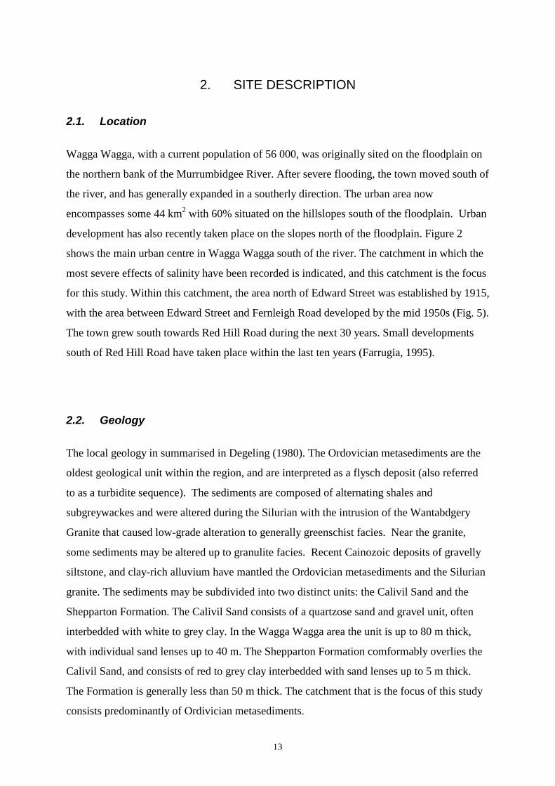
The depth to the water table varies from more than 10 m near Willans Hill, to less than 2 m in

the Emblem Park area, where salinity has affected urban infrastructure and vegetation (Fig. 4).

Hydraulic measurements within this part of the catchment show an upward pressure gradient

of approximately 0.02 – 0.03. Groundwater modelling (Paul et al., 1996: Paul, 1997) indicated

a potential for reducing deep groundwater pressures and lowering the shallow water table in

salinised areas by groundwater pumping. In July 1998, ten dewatering bores were drilled

within an area of approximately 35 hectares bounded by Cullen Road, Chaston Street, Docker

Street and Edward Street. The bores represent a pilot project to determine the effectiveness of

aquifer dewatering for lowering water tables beneath the urban area. One of the bores (Bore 9)

had a very low hydraulic conductivity, presumably because it did not intersect any significant

fracture zones. The remaining nine bores were equipped with pumps, and the pumps were

turned on 1st November 1999. Between 1st November 1999 and 18th December 2000 a total of

113 ML of water was pumped from the aquifer (100 ML/yr), at a mean pumping rate (per

bore) of 0.35 L/s (WWCC, 2001). Discharge from the pumping scheme is discharged directly

into the Murrumbidgee River. A license from the Murray Darling Basin Commission allows

the discharge of up to 1.12 tonnes/day of salt into the river. At a pumping rate of 100 ML/yr,

this equates to a mean salinity of 4090 mg/L.

Paul et al. (1996) describes results of a seven-day pumping test carried out on one of the

dewatering bores located in the northern part of the catchment. The pumping bore, screened

within the Ordivician metasediments, was pumped at approximately 0.5 L/s, and water levels

were recorded in the pumping well, and in seven observation wells. Analysis of the drawdown

in the observation wells indicated that the vertical hydraulic conductivity was much greater

than the horizontal hydraulic conductivity. Transmissivity values measured from pumping

tests carried out on each of the dewatering bores, all of which are screened within the

metasediments (18 m screen lengths), ranged between 0.8 and 48 m2/day, with most values

between 4 and 9 m2/day (Carter, 1998).

17

Figure 4. Depth to groundwater. Circles denote piezometers that were used to construct the map.

18

3. METHODS

3.1. Water sampling and analyses

3.1.1. Rainfall sampling

Rainfall collection stations were set up in November 1999 at the Bushfire Depot, Fernleigh

Road, and at the old gas works in Chaston Street. In December 2000, the collection station in

Chaston Street was moved to the Environmental Health Depot, Glenfield Road, due to

demolition at the old gas works site. The locations of these stations are shown in Figure 5.

Two rainfall gauges were located at each site: a standard raingauge, and a thistle funnel

collector. The thistle funnel collector was used for collection of rainfall samples for

measurement of 18O and 2H. A layer of kerosene was used to prevent evaporation from the

funnel, and rainfall was collected at approximately weekly intervals through the tap at the

bottom of the funnel. These samples are being archived, and have not yet been analysed. The

standard raingauge was used for collection of samples for major ion analysis. After each

rainfall event, rain that had collected in the gauge was transferred into a 1 litre glass container.

At approximately monthly intervals, the 1 litre container was subsampled and emptied. These

samples were analysed for chloride and major ions. Results of chloride analyses are presented

in Appendix 1.

3.1.2. Reticulated water sampling

Twelve water samples were collected from the reticulated water system, and analysed for

major ions, 2H and 18O. There are two borefields that supply water to the Emblem Park areas.

“East Wagga” consists of three bores, two of which were being used at the time of sampling

(July - August 1999). “West Wagga” consists of five bores, four of which were being used.

Each of the operational bores was sampled at the borehead, and three samples were collected

from the reticulation of each system. Samples were analysed for ion chemistry, 18O and 2H.

Results are given in Appendix 2.

19

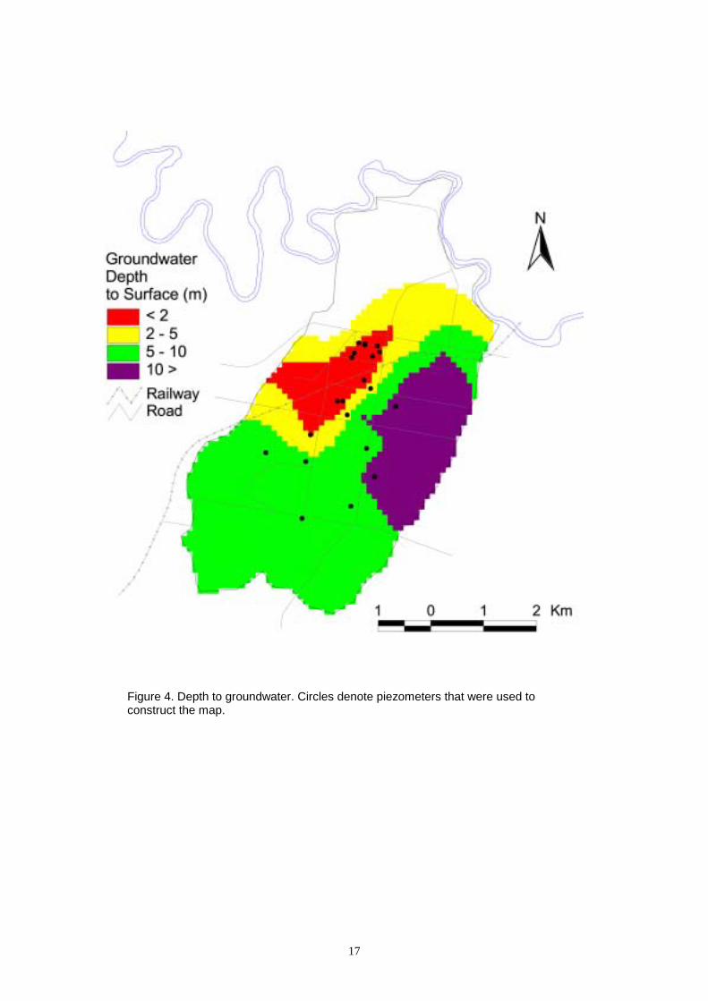
3.1.3. Groundwater sampling

Groundwater samples were collected after purging at least two well volumes from each

piezometer. The bores sampled, their total depth and the average depth of the water table for

each is listed in Table 1. The bore locations are shown in Figure 5. Samples were analysed for

major ions, 14C, 13C, 2H and 18O, and the results are given in Appendix 3. Samples for radon

analysis were collected from within the well screens of the piezometers before purging, as

well as after purging.

Figure 5. Locations of rainfall and groundwater sampling sites. Letters denote rainfall collectors (A: old gas works; B: Environmental Health Depot; C: Bushfire Depot), and numerals denote bore identification numbers.

20

Table 1. The total bore depth, and the mean depth to the water table (before pumping) of piezometers sampled in this study. The bottom 1 – 2 m of each piezometer is slotted. Exceptions are Emblem 1/2, 2/2, 1/3 and 3/3, that have 6, 6, 10 and 10 m screens, respectively.

Bore No. Depth (m) SWL (m)

Emblem 1/1 15 2.9 Emblem 1/2 30 2.2 Emblem 1/3 60 1.5 Emblem 2/1 15 2.3 Emblem 2/2 30 1.9 Emblem 2/3 60 1.5

4 3.30 0.84 5 9.70 3.51 6 13.20 11.49 7 3.90 2.78 9 4.30 0.07 10 4.10 0.91 11 7.10 5.16 19 17.20 11.85 34 24.00 7.42 37 40.00 8.35 38 15.00 8.74 42 12.60 1.87 43 17.28 6.60 44 22.54 12.73 47 16.27 13.24 59 3.00 1.34 67 3.00 1.05 68 3.00 1.93 69 3.00 2.09 90 6.60 1.00

3.1.4. Water analyses

Water samples for major ion analyses were pre-filtered in the laboratory using a 0.45 µm

membrane filter. 2H/1H and 18O/16O ratios were measured on water molecules using mass

spectrometric techniques described by Dighton et al. (1997) and Socki et al. (1992),

respectively. All values are reported relative to the Vienna-Standard Mean Ocean Water

(V-SMOW) standard, using the per mille (‰) notation according to:

δ = [{Rsample/Rstandard}-1] ×1000 (1)

where Rsample is the isotope ratio of the sample and Rstandard is the isotope ratio of the V-

SMOW standard. 14C activities and 13C/12C ratios were analysed on dissolved inorganic

carbon precipitated from 20 – 60 litre water samples as BaCO3. The 14C activity was

21

determined using the direct absorption technique (Leaney et al., 1994) and analysed on a low

level LKB Wallac Quantulus liquid scintillation counter. An aliquot of the CO2 was analysed

for δ13C and expressed as delta notation as indicated above, using standard PDB as the

reference. The radon concentration is counted in the laboratory by liquid scintillation, on a

LKB Wallac Quantulus counter using the pulse shape analysis program to discriminate alpha

and beta decay (Herczeg et al., 1994).

3.2. Fracture mapping

In order to interpret the fracture orientation in the Ordovician metasediments, a survey of

outcrops around the Wagga area was conducted. The outcrops weather fairly quickly and it is

difficult to find large sections of clean outcrop. Near the surface, the effects of creep on these

outcrops can be seen altering the density and orientation of the fractures. More detailed work

for fracture characteristics would be difficult in this formation.

Three of the best-exposed sites were surveyed to determine the number and orientation of

fracture sets in the formation. One is located off Baden Powell Drive (near Willans Hill) and

is a small tunnel constructed for a model railroad track. The second is the Southern Roadbase

Quarry located off Red Hill Road (Fig. 2). The third site is a disused quarry located in

Pomingalarna Park off Sturt Highway west of Wagga. With the poor quality of the outcrops,

scanline techniques were not used. Instead, multiple measurements from all observed fracture

sets were taken with a geological compass to determine the orientation of the fracture planes.

The measurements were converted to grid north using a 12 degree correction. With this

technique, some of the variability of the fracture orientation can be characterised, but

quantitative data on fracture density is not available. Qualitative observations were made in

an attempt to generate preliminary hypotheses regarding which fracture set may be the most

permeable.

22

3.3. Groundwater modelling

Simple catchment scale groundwater modelling was carried out using an analytical solution to

the one-dimensional advection-dispersion equation

RxhKh

thS +

∂∂=

∂∂

2

2

(2)

where K is the aquifer hydraulic conductivity, h(t,x) is the hydraulic head, S is the specific

yield, R is the recharge rate, t is time and x is distance. In order to solve the equation we have

assumed that the specific yield, S, and aquifer transmissivity T=Kh are constant. Boundary

conditions are

0== xatkh (3)

Lxatxh ==

∂∂ 0 (4)

We define

0=∂∂= xat

xhTtQ )( (5)

The initial condition is

( )

−−=

221

21

Lx

Lx

TLRkxh (6)

where h(x) describes the steady state head distribution for a recharge rate of R1. For an

instantaneous change in recharge rate from R1 to R2 at time t=0, the solutions for the hydraulic

head h(t,x) and aquifer discharge Q(t) become

( ) ( )( )

( )( )

+−

+

+

−+

−+= ∑

∞

=t

SLTn

nLxn

RRTLxLx

TRkxth

n2

22

03213

222

412

122

1216

2π

π

πexp

sin, (7)

23

and

( ) ( ) ( )

( )∑∞

= +

+−

−+=0

2

2

22

221

2 124

128

n n

tSL

TnRRLLRtQ

π

π

exp (8)

Solutions for more general step changes in R(t,x) can be readily calculated, and a FORTRAN

program was written for this purpose.

Due to the high apparent anisotropy suggested by the fracture mapping, three-dimensional

modelling of the dewatering trial site was carried out using a model that could simulate both

vertical and horizontal anisotropy. Previous groundwater modelling to predict the success of

groundwater pumping has been carried out using MODFLOW (Paul et al., 1996; Paul, 1997).

However, these simulations have not considered radial anisotropy of hydraulic conductivity,

in part because MODFLOW is not well-suited to such situations. We have attempted to

predict the likely direction of anisotropy within the bedrock by mapping the orientation of

fractures in available outcrops within the catchment. Numerical simulations were then carried

out using FRAC3DVS. FRAC3DVS is a three-dimensional discrete fracture model capable of

simulating steady state or transient, saturated or unsaturated flow in fractured or unfractured

porous media. The variably saturated flow equation is solved using a control volume finite-

element method. An exhaustive description of FRAC3DVS, including mathematical

development is found in Therrien and Sudicky (1996). In this report, simulations are carried

out in porous media mode, but incorporating anisotropy of hydraulic conductivity.

24

4. GROUNDWATER RECHARGE

4.1. Recharge prior to development

According to Swan (1970), the original vegetation of the Wagga Wagga district was savanna

woodland. There are no significant areas of native vegetation remaining within the catchment,

other than Willans Hill. However, prior to the growth of the town, this would have been the

only source of recharge in the catchment.

Chloride concentrations of groundwater samples vary between 320 and 8560 mg/L, with a

mean of 1855 mg/L. The mean chloride concentration of deep groundwater samples is 720

mg/L, with six of the eight deep samples having chloride concentrations between 300 and 600

mg/L. (Deep groundwater samples have been defined to be those where the bore depth is at

least 12 m below the mean water table position.) The deep groundwaters were likely

recharged under native vegetation, and should pre-date development. Blackburn and McLeod

(1983) measured the mean chloride concentration in 1974/75 rainfall at Wagga Wagga to be

1.2 mg/L. Over the 15-month period between December 1999 and February 2001, we have

measured the mean chloride concentration in rainfall to be 1.06 mg/L. If we assume a value of

1.2 mg/L for the long-term chloride fallout, then we can use the chloride concentration of deep

groundwater to estimate the recharge rate under native woodland vegetation, using a chloride

mass balance:

RCPC RP = (9)

where CP and CR are the chloride concentrations of precipitation and of the groundwater,

respectively, and P and R are the mean annual rates of precipitation and recharge (Allison and

Hughes, 1983). Substituting using CP = 1.2 mg/L, P = 550 mm/yr and CR = 500 mg/L, we

calculate a mean recharge rate of approximately R = 1.3 mm/yr. This is consistent with

measurements of recharge rates beneath wooded land in other parts of the Murray Basin (e.g.,

Kennett-Smith et al., 1992). Based on a catchment area of 27 km2, this represents a volumetric

recharge rate of 35 ML/yr.

25

4.2. Recharge beneath agricultural land

The southern portion of the catchment is agricultural land, and diffuse recharge occurring here

would move north, underneath the urban area, to discharge to the Murrumbidgee River.

Within recent years, the growth of the town has decreased the area of agricultural land.

The recharge rate under agricultural land has not previously been determined, and we were

unable to locate any bores within this portion of the catchment. However, comparison with

studies in other parts of the Murray Darling Basin (Kennett-Smith et al., 1994), suggests that

the rate of recharge beneath agricultural land may be approximately 15 mm/yr, which is just

under 3% of the mean annual rainfall. Water tables are rising beneath most of the agricultural

areas surrounding Wagga Wagga. Within the Ordivician slate, the median rate of water table

rise is 0.34 m/yr (Lytton et al., 1993). This is consistent with a recharge rate of 15 mm/yr, and

specific yield of 0.04.

4.3. Urban recharge

Within the urban area, several distinct sources of groundwater recharge can be identified:

• Diffuse urban recharge. Diffuse urban recharge results from infiltration of rain falling on

parks, gardens and lawns. In some areas, this recharge will be enhanced by irrigation.

• Rubble pits. The direction of roof runoff into rubble pits was a method used in Wagga

Wagga prior to the mid-1970s for houses on the low side of the street that could not drain

their roof water into the street stormwater system. These rubble pits provide a mechanism of

direct recharge to groundwater.

• Pipe leakage. Leakage from water supply and sewerage pipes is a potential source of direct

recharge to the aquifer.

Hamilton (1995) made some preliminary estimates of the volumes of recharge that might be

contributed through the various sources within a 425 hectare area of the urban catchment. The

study area included 1800 residences, a commercial area and a number of education and

26

government institutions. Water usage for the twelve-month period from August 1993 to July

1994 was obtained from Southern Riverina Electricity and Water. Actual rainfall for this

period was 700 mm, which is 150 mm above the annual average. The total volume of

reticulated water supplied to this study area was 892 500 kL. Hamilton’s estimates of recharge

volumes are given in Table 2. Hamilton assumed that 3% of rain falling on areas which were

not paved or rooved (68% of the land area) recharged the aquifer. Application rates of

irrigation water averaged 240 mm for domestic gardens (53% of domestic water use) and 660

mm for public recreation areas. The author assumed that 30% of total water use by various

government authorities within the region was used for irrigation, giving a total irrigation

volume for all users of 411 500 kL. Hamilton assumed that between one and two percent of

the irrigation water recharged the aquifer, giving a total recharge from irrigation of 4120 –

8240 kL. Within the study area, 23% of houses have rubble pits. Using an average roof area

of 186 m2, and assuming that all rainfall onto the roof area reaches the rubble pits, this gives a

volume of recharge of 53 120 kL. Assuming a pipe leakage of 5% through the Southern

Riverina Electricity and Water supply system gives a recharge rate from this source of 46 400

kL. However, this figure does not include leakage that occurs in the individual customers

homes (between the water meter and the point of use). Using an average value of 17%

obtained from a 1993 NSW Water Supply and Sewerage Performance Comparisons, put out

by the Public Works Department, this gives a potential recharge from pipe leakage of 157 800

kL (apparently misreported as 190130 kL in Hamilton (1995) and Paul et al. (1996).)

Table 2. Estimates of recharge volumes (kL) to a 425 hectare urban area for the twelve month period between August 1993 and July 1994. The last column gives estimates of annual mean recharge volumes. Numbers in parentheses represent recharge rates in units of mm/yr.

Hamilton (1995) Paul et al. (1996) Nash (1999) This study Total Rainfall 2 975 000 Total Reticulated Supply 928 270 824 000 Diffuse recharge – rainfall 59 500 29 750 – 89 250 47 685 (11) Diffuse recharge - irrigation 4120-8240 4120 – 20 600 8 240 (2) Diffuse recharge - TOTAL 63 620 – 67 740 63 620 – 109 850 55 925 (13) Rubble pits 53 120 53 120 53 120 (12) Pipe leakage – council 41 200 Pipe leakage – landholder 12 420 Pipe leakage – water supply

46 400-157 800 46 400 – 157 800 53 620 53 620 (13)

Pipe leakage – sewer Not quantified 16 430 – 49 280 16 430 (4) TOTAL RECHARGE 234 960 (55)

27

Paul et al. (1996) and Nash (1999) revised some of the estimates of Hamilton (1995). In

particular, Paul et al. (1996) estimated a leakage volume from the sewer system, based on 5-

15% leakage of a sewerage volume of 200 L/day/person. Paul et al. (1996) also revised

upward the estimate of diffuse recharge from irrigation (from 1-2% to 1-5% of applied water).

Leak detection exercises undertaken in Turvey Park in 1998 by Riverina Water showed mains

and service leaks to be in the order of 5 percent, and a typical household leak of around 2

percent. Nash (1999) revised the estimates of pipe leakage using this data, and also used a

revised estimate of the total reticulated water supplied to the study area over the relevant

twelve-month period.

The final column in Table 2 gives our best-estimates of the catchment water balance, based

largely on the earlier work of Hamilton (1995), Paul et al. (1996) and Nash (1999). We have

used 3% of rainfall for the diffuse recharge from rainfall, as per Hamilton (1995), but have

reduced the volume proportionally to correct for the very wet year studied by Hamilton. (The

increase in irrigation which may arise in a drier year has not been corrected for, but is not

considered to be significant.) We have assumed that only 2% of irrigation water recharges the

aquifer, which was the upper bound of the range given by Hamilton (1995), and towards the

lower end of the range given by Paul et al. (1996). We have taken the value of water supply

pipe leakage given by Nash (1999), and the figure for sewerage pipe leakage given by Paul et

al. (1996). Summing the various contributions, gives a total recharge of 234 960 kL/yr, which

is equivalent to 55 mm/yr.

4.4. Identifying urban recharge

4.4.1. Recharge end-members

The chemical composition of the groundwater will reflect that of the various recharge sources,

modified in some cases by chemical reactions that may occur within the aquifer.

28

Recharge beneath agricultural land. Diffuse agricultural recharge should have a chemical

composition similar to that of rainfall, but with higher concentrations of conservative ions due

to evaporative enrichment.

Diffuse urban recharge. Diffuse urban recharge results from infiltration of rain falling on

parks, gardens and lawns. In some areas, this recharge will be enhanced by irrigation using the

reticulated water supply. The chemical signature of diffuse urban recharge would thus be

between that of rainfall and that of reticulated water, with concentration by evaporation.

However, most recharge is likely to occur during winter when irrigation is less, and so a

chemical signature closer to evaporated rainfall is most likely. This source of recharge may

also contain elevated concentrations of nitrate, from the addition of fertilisers to lawns and

gardens.

Rubble pits. Recharge via rubble pits should have a chemical signature similar to that of

rainfall, with little evaporation.

Pipe leakage. Pipe leakage should have a chemical signature similar to that of the reticulated

water supply. Leakage from the sewerage system may have elevated concentrations of nitrate

and some other ions.

The chemical composition of reticulated water, groundwater, river water and rainfall samples

are shown in Appendix 1-3. The reticulated water is sourced from bores located in the

floodplain of the Murrumbidgee River, and the chemical composition of this bore water

closely resembles that of the river. Water treatment includes the addition of sodium silicate

and aluminium sulphate as flocculants. The process reduces the turbidity of the water,

precipitating aluminium hydroxide in the process. Calcium hydroxide is then added to

increase the pH, and chlorine is added to kill any remaining bacteria. Finally, sodium silico

fluoride is added to raise the fluoride level of the water to approximately 1 mg/L (Southern

Riverina Electricity and Water, 1994).

The chemical treatment of the reticulated water results in it having a very different chemical

composition from rainfall recharge. In particular, Si/Cl, F/Cl and HCO3/Cl ratios are usually

much higher in reticulated water than in groundwater. However, determination of the

29

proportions of rainfall and reticulated water in groundwater samples from dissolved ion

concentrations is complicated because:

1. The chemical composition of most of recharge sources is not well known. In particular,

amount of evaporation during diffuse groundwater recharge is uncertain, and likely to be

spatially variable.

2. Some ions can be added from rock weathering, and may also be involved in ion exchange

processes.

3. Further concentration of ions can occur at various points along the flowpath during

evaporation from shallow water tables

In particular, because of the high concentration of salts in rainfall recharge relative to those in

recharge from reticulated water (particularly pipe leakage, which would not undergo any

evaporation prior to recharge), concentrations of individual ions are unlikely to be useful.

(Concentrations of most ions in reticulated water are small relative to concentrations in

groundwater, and so they cannot be used as markers.) In the following sections, we compare

concentrations of some key ions and isotopes in reticulated water and in groundwater.

4.4.2. Chloride

Chloride concentrations in shallow groundwater are much greater than those in deep

groundwaters. This may be attributable to evaporative concentration, although it is also

possible that there is a source of salt in the shallow soils that has been mobilised by the rising

water table. In most cases, urban recharge would be expected to reduce chloride

concentrations, although sewerage leakage may contain elevated concentrations (Vengosh and

Pankratov, 1998)

30

4.4.3. Stable isotopes of water

Figure 6 depicts the water stable isotope ratios of shallow and deep groundwaters, and of the

reticulated water supply. The deep groundwaters fall on a line with slope of approximately

eight, and this likely reflects the local meteoric water line. Shallow groundwaters have higher 2H and 18O concentrations than the deep groundwaters, and mostly fall to the right of the local

meteoric water line, probably indicating evaporative enrichment. Samples of reticulated water

are only slightly more depleted than the deep groundwaters. Because of the similarity of the

stable isotopic composition of the deep groundwaters and the reticulated water supply, and

because of the large change in composition due to evaporative enrichment, the water stable

isotopes do not appear to be useful for distinguishing the different recharge sources.

-8 -7 -6 -5 -4-50

-45

-40

-35

-30

-25

Reticulated SupplyShallow GroundwaterDeep Groundwater

2

18

H (‰

)

O (‰)

Figure 6. Stable isotope ratios of shallow and deep groundwaters and of the reticulated water supply. The solid line is the global meteoric water line. The broken line is the probable local meteoric water line.

4.4.4. Carbon-14 and HCO3

Figure 7 plots 14C concentrations versus the molar HCO3/Cl ratio in groundwater samples.

Reticulated water samples collected as part of this study have a HCO3/Cl ratio of

approximately 2.0. No reticulated water samples have been analysed for 14C, but they should

have an activity close to 100 pmc. The HCO3/Cl ratio in groundwater is increased by rock

weathering, but is not affected by evaporation. For most groundwater samples, the HCO3/Cl

31

ratio increases as aquifer residence time increases. The data suggests an exponential

relationship between 14C and HCO3, which might indicate the addition of HCO3 from rock

weathering. If the differences in 14C activity were solely due to radioactive decay, no such

relationship should exist. The samples from wells 19 and 38 are distinct from the rest of the

data, and have very high HCO3/Cl ratios, despite being very young. The high HCO3/Cl ratio is

evidence that reticulated water is a major source of recharge at these sites. However, because

HCO3/Cl ratios in groundwater and reticulated water differ by only a factor of 10, and because

chloride concentrations in groundwater exceed those in reticulated water by a factor of 100,

HCO3/Cl ratios are not very sensitive to the addition of reticulated water.

0

20

40

60

80

100

0 0.2 0.4 0.6 0.8 1.0 1.2 1.4

HCO /Cl (molar ratio)

C (p

mc)

19

3

14

38

addition of HCO

decay

3

Figure 7. 14C concentrations of groundwater samples versus the molar HCO3/Cl ratio. The latter is increased by rock weathering, but is not affected by evaporation. The figure shows that HCO3 concentrations increase as aquifer residence time increases. The samples from wells 19 and 38 are distinct from the rest of the data, and have very high HCO3/Cl ratios, despite being very young. The high HCO3/Cl ratio is evidence that reticulated water is a major source of recharge at these sites.

4.4.5. Nitrate Groundwaters obtained from deep bores have nitrate concentrations less than 2 mg/L, and

concentrations in the reticulated water supply are less than 1 mg/L. However, elevated

concentrations (5.0 - 10.4 mg/L) have been observed in several shallow groundwater samples.

These presumably indicate anthropogenic influences, and may reflect either addition of

32

fertiliser to lawns, parks and gardens, or leakage from the sewerage system. However, because

nitrate is not conservative in the subsurface, the absence of nitrate does not indicate an

absence of recharge from these sources.

4.4.6. Fluoride and silica ratios

Dissolved silica that is naturally present in groundwater is derived from weathering of primary

silicate minerals such as plagioclase feldspar. Very little is derived from weathering of quartz

due to its low solubility. Silica concentrations seldom reach that of saturation with respect to

amorphous silica (about 2 mmol/L at 25°C). This is thought to be caused by secondary

reactions involving clay minerals that are ubiquitous in aquifers. These reactions buffer silica

concentrations in most groundwaters between 0.15 to 0.45 mmol/L.

Silica concentrations in deep groundwater samples at Wagga show a weak positive correlation

with Cl, (due to evaporation) but the Si/Cl ratio decreases due to removal of Si to secondary

clay minerals that occurs with increasing TDS concentrations in the soil zone and

groundwater (Fig. 8). For example, the reaction:

3.5Al2Si2O5(OH)4 + Na+ + 4H4SiO4 = 3 Na0.33Al2.33Si3.67O10(OH)2 + H+ + 11.5H2O

kaolinite montmorillonite

proceeds to the right (consuming SiO2) within increasing concentration of the water as it

transits through the soil zone. Silica concentrations in deep groundwater range between 0.164

and 0.196 mmol/L with Si/Cl ratios between 0.003 and 0.02 (Fig. 9).

Fluoride is a halide (like Cl-) but behaves differently in waters due to its very high

electronegativity. It has a similar ionic radius to OH- and therefore substitutes readily onto

hydroxyl sites of clay minerals. The decrease in F- concentration with increasing Cl-

concentration of Wagga deep groundwaters (Fig. 8) suggests that there is a source of F- in the

dilute waters (possibly via dissolution of the mineral apatite which is common in sediments

derived from granitic rocks), and that this is rapidly removed onto clays during transit through

33

the soil zone. Fluoride concentrations in deep groundwater range between 0.026 and 0.12

mmol/L with F/Cl ratios between 4.7 × 10-4 and 1.4 × 10-2.

Fluoride and silica are both added to the reticulated water as part of the treatment process, and

since they are present in relatively low concentrations in deep groundwater, this raises the

possibility of them being useful tracers of recharge from reticulated waters (particularly pipe

leakage). Reticulated water samples have silica concentrations between 16 and 19 mg/L, and

Si/Cl ratios between 0.4 and 1.9. Fluoride concentrations of reticulated supply bores range

between 0.2 and 0.7 mg/L (F/Cl = 0.018 – 0.062) , which is increased to between 0.8 and 1.1

mg/L in the reticulated supply (F/Cl = 0.035 – 0.072). F/Cl and Si/Cl ratios of shallow

groundwater are distinct from deep groundwater, which may indicate the presence of urban

recharge, and specifically the addition of reticulated water.

0

0.15

0 10 20 30 40 60

0.10

0.05

500.10

0.12

0.14

0.16

0.18

0.20

Cl (mmol/L)

Si (m

mol

/L)

F (m

mol

/L)

Figure 8. Silica and fluoride versus chloride plots for deep groundwaters.

34

If we assume that evaporative enrichment occurred subsequent to any mixing with urban

recharge or geochemical reactions within the aquifer, then we can estimate the proportion of

reticulated water in groundwater samples based on their F, Si and Cl concentrations. We

assume that an unknown fraction, f, of reticulated water is added to the diffuse rainfall

recharge. The source of this reticulated water could be from pipe leakage, or from irrigation

recharge. We can then write the mixing equation:

X[gw] = e{(1-f) X[recharge] + f X[reticulated]} (10)

where e denotes a concentration factor during the final evaporation process, and X[gw],

X[recharge] and X[reticulated] are concentrations of ion X in the groundwater, in diffuse

rainfall recharge and in reticulated water. We assume that diffuse recharge from rainfall has a

chloride concentration of 500 mg/L, which is close to the mean chloride concentration

measured in deep bores. In order to solve for f, we assume a relationship between silica and

fluoride concentrations of deep groundwaters given by the straight line in Figure 9. The

equation for this relationship is:

F[recharge] / Cl[recharge] = -0.0058 + Si[recharge] / Cl[recharge] (11)

Thus equation 10 for Cl, Si and F together with equation 11 yields four equations with four

unknowns (e, f, F[recharge] and Si[recharge]), and so can be uniquely solved. The implicit

assumption with this method, is that there are no further chemical processes which alter

fluoride and silica concentrations after addition of reticulated water, and subsequent

evaporative enrichment during groundwater discharge. The values of f estimated using this

approach are given in Table 3.

35

Si/Cl

F/C

l

deep

gro

undw

ater

s

Shallow GroundwaterDeep Groundwater

0 0.02 0.04 0.06 0.08 0.10

0.002

0.004

0.006

0.008

0.010

0.012

0.014

Figure 9. Silica/chloride and fluoride/chloride molar ratios for deep and shallow groundwaters.

Table 3. Fractions of reticulated water in groundwater samples, as derived from chloride, fluoride and silica concentrations. Nitrate concentrations and 14C activities are shown for comparison.

Well Number Fraction of Reticulated Water

NO3-N (mg/L)

14C (pmC)

19 0.68 5.3 91.5 11 0.55 5.01 38 0.26 10.4 90.3 4 0.24 0 5 0.15 0 95.9

42 0.15 0 92.1 47 0.15 0, 4.6 44 0.11 0 10 <0.1 0 34 <0.1 0 86.9 7 <0.1 0 6 <0.1 0 9 <0.1 0

37 <0.1 0 46.9 43 <0.1 7.4 90.1 90 <0.1 0

Emblem 1/1 <0.1 1.3 47.8 Emblem 1/2 <0.1 1.8 37.8 Emblem 1/3 <0.1 0.9 29.8 Emblem 2/1 <0.1 1.8 48.1 Emblem 2/2 <0.1 1.5 35.5 Emblem 2/3 <0.1 1.2 29.1

59 0 67 0 68 0 69 1.6

36

4.4.7. Summary

Several tracers were found to have some potential for determining sources of urban recharge.

These included: (i) 14C versus HCO3 plots, (ii) NO3 concentrations, and (iii) ratios of F, Si and

Cl. Despite their differences, good agreement was generally found between the different

methods. For example, the three wells with the highest fractions of reticulated water as

determined by F, Si and Cl, all have nitrate concentrations above 5 mg/L. The only other well

with high nitrate that does not appear to have any reticulated water, based on its fluoride and

silica concentrations, is well 43. It is possible that the high nitrate in this well is due to a very

small leakage from the sewerage system, such that the volume of water involved is not

sufficient for it to be distinguished using F, Si and Cl ion ratios. Of course, some forms of

urban recharge (such as water supply pipe leakage) would not be expected to contain high

nitrate levels. Also denitrification may reduce NO3 levels in the subsurface. Thus while high

nitrate concentrations may be an indicator of urban recharge, low nitrate levels cannnot be

taken as evidence of non-urban sources.

All wells with measurable reticulated water based on F, Si and Cl concentrations, have 14C

activities above 90 pmC. The only other well with a 14C activity above 90 pmC is well 43,

which also has a high NO3 concentration.

Better discrimination of the recharge sources would be aided by more accurate determination

of end-members, and in particular, by accurate measurement of chloride, silica and fluoride

concentrations in rainfall. Further discrimination of recharge sources may also be possible

using additional tracers. In particular, nitrogen isotopes (15N/14N) may help distinguish

between irrigation recharge (fertilisers) and sewerage pipe leakage. Boron isotopes may also

help distinguish sewerage pipe leakage.

All of the deep groundwater samples were found to contain little or no reticulated water (less

than 10%). Of the 14 shallow wells for which analyses were available, 8 had a significant

component of reticulated water. Two of these were found to comprise mainly water from the

reticulated supply (wells 19 and 11). Bores that show evidence of urban recharge are mostly

located in the upland areas. North of the railway line, even shallow bores show no evidence of

urban recharge. This supports the suggestion that the water table has always been close to the

land surface in this area. It also suggests that urban recharge is not presently occuring here,

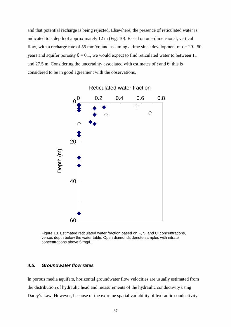
37

and that potential recharge is being rejected. Elsewhere, the presence of reticulated water is

indicated to a depth of approximately 12 m (Fig. 10). Based on one-dimensional, vertical

flow, with a recharge rate of 55 mm/yr, and assuming a time since development of t = 20 - 50

years and aquifer porosity θ = 0.1, we would expect to find reticulated water to between 11

and 27.5 m. Considering the uncertainty associated with estimates of t and θ, this is

considered to be in good agreement with the observations.

Reticulated water fraction

60

40

20

0

Dep

th (m

)

0.60.40.20 0.8

Figure 10. Estimated reticulated water fraction based on F, Si and Cl concentrations, versus depth below the water table. Open diamonds denote samples with nitrate concentrations above 5 mg/L.

4.5. Groundwater flow rates

In porous media aquifers, horizontal groundwater flow velocities are usually estimated from

the distribution of hydraulic head and measurements of the hydraulic conductivity using

Darcy’s Law. However, because of the extreme spatial variability of hydraulic conductivity

38

observed within fractured rock systems, hydraulic conductivity values measured at small

scales may be of little practical value for determining regional scale groundwater flow rates. In

fractured rocks, point dilution methods have proven more reliable for quantifying groundwater

flow rates. Here, we estimate groundwater flow rates from radon concentrations within the

aquifer, using a modification of the point dilution method that is most suitable for measuring

very low flow rates.

Cook et al. (1999) and Hamada (1999) showed that the ratio of radon concentrations measured

before purging to those measured after purging was an indication of the horizontal

groundwater flow rate. Where groundwater flow rates are very low, the radon concentration in

the well before purging will be much lower than that in the aquifer, due to radioactive decay

of radon during flow through the well. Conversely, if the flow rate is very high, negligible

decay will occur during flow through the well, and the ratio will be close to one (Fig. 11).

0.1 1 10 1000.01

0.1

1

0C

/ C

Flow (m/yr)

Figure 11. Theoretical relationship between radon concentration in an unpurged borehole, relative to that in the aquifer, and groundwater flow rate, for a bore radius of 0.1 m. (After Cook et al., 1999.)

However, because the well usually constitutes a local high hydraulic conductivity zone,

convergence of groundwater flowlines near the well will mean that the flow rate within the

well, per unit area, will be greater than the flow rate within the aquifer. The magnitude of this

39

effect will vary with the bore geometry (bore and well screen radius), and with the hydraulic

conductivity of the aquifer and the gravel pack (if present). The effect can be quantified for

particular situations, and usually ranges between two and four times.

Radon concentrations measured both before and after well purging are shown in Table 4.

(Radon concentrations after purging were not measured in several piezometers, because their

low hydraulic conductivity meant that purging took several days, over which time significant

decay of radon would have occurred.) Concentrations measured after purging range between

28 and 450 Bq/L. The variability probably primarily reflects variation in the uranium content

of aquifer materials adjacent to the bores screens.

Table 4. Concentrations of 222Rn in groundwater measured before and after well purging.

222Rn (Bq/L) Well Date Sampled Before Purging After Purging

9 15.05.00 3.3 10 15.05.00 0.0 19 15.05.00 10.8 37 12.01.99 126.4 123.5 38 12.01.99 5.1 42 15.05.00 2.5 28.4 43 15.05.00 2.2 81.8 44 15.05.00 21.9 294.0 47 15.05.00 4.2 90 11.01.99 13.5

Emblem 1/1 12.01.99 5.9 Emblem 1/2 12.01.99 96.3 109.1 Emblem 1/3 12.01.99 116.5 138.9 Emblem 2/1 12.01.99 379.3 Emblem 2/2 12.01.99 197.7 Emblem 2/3 12.01.99 447.4

Figure 12 shows purged and unpurged radon concentrations as a function of depth below the

land surface. Although it is possible that unpurged radon concentrations from the piezometers

in Emblem Park have been influenced by pumping, Figure 12 suggests that unpurged

concentrations are significantly less than purged concentrations in the upper part of the

aquifer, but that unpurged and purged concentrations have similar values at depth. This is

consistent with greater weathering of the shallower metasediments. Shales tend to weather to

clays, with reduced hydraulic conductivities. The data suggests a mean value of C/C0 of 0.02 –

40

0.05 above 20 m depth, and C/C0 > 0.8 at depth. Although only a relatively small number of

bores have been sampled, the results suggest groundwater flow rates of 0.2 – 0.6 m/yr close to

the water table, but in excess of 40 m/yr at depth. (It should also be noted that screen locations

of deeper piezometers may be preferentially located on higher flow zones.)

Radon (Bq/L)

60

40

20

0

Dep

th (m

)

101 1000100

Figure 12. Unpurged (open circles) and purged (closed circles) radon concentrations versus depth of piezometer screen below the land surface.

41

5. GROUNDWATER DISCHARGE

5.1. Natural groundwater discharge

Prior to development, the catchment recharge rate is estimated to have been 35 ML/yr, and

this would have been balanced by a natural discharge to the river of 35 ML/yr. There is some

suggestion that the water table in the Emblem Park area was close to the land surface before

development, suggesting that this was close to the discharge capacity of the catchment.

Today, approximately one-quarter of the catchment is agricultural land, and three-quarters is

urban. Based on recharge rates of 15 mm/yr and 55 mm/yr for agricultural and urban land

respectively, and a catchment area of 27 km2, the current catchment recharge is estimated to

be 1215 ML/yr. A proper understanding of the current groundwater balance is hampered by a

lack of monitoring bores with long periods of observation. No water level records greater than

six years are available, and many bore records are much shorter than this. Nevertheless, the

limited available information suggests that water levels are not currently rising, and hence the

catchment has reached (or is close to) a new steady-state condition. Thus, groundwater

discharge must be 1215 ML/yr.

In the low part of the catchment, the gradient towards the river is approximately 0.002 - 0.004,

and the width of the catchment is approximately 3 km. The mean aquifer transmissivity, T,

required to discharge 1215 ML/yr of water can be calculated from a rearrangement of

xhwTQ

∂∂= (12)

where Q is the catchment discharge, w is the catchment width, and ∂h/∂x is the hydraulic

gradient. Solving for T gives T = 275 - 550 m2/day. Measured values of transmissivity in the

Emblem Park area (see Section 2.3) mostly range between 4 and 9 m2/day. These tests were

conducted over well screen intervals of 18 m. Assuming an aquifer thickness of 100 m, these

equate to aquifer transmissivities of 22 – 50 m2/day, which is significantly less than calculated

using Equation 12. There are a couple of possible reasons for this. The first involves the scale

effect of hydraulic conductivity. Hydraulic conductivity values measured in small-scale

42

pumping tests may not intersect the largest fractures, which may be important for flow at

regional scales. Secondly, urban areas are usually characterised by a network of shallow

trenches that are constructed for water and sewerage pipes, and often also for telephone and

electricity cables. These trenches are often backfilled with material that has a higher hydraulic

conductivity than the surrounding aquifer material, and so can form preferential flowpaths

(Sharp, 1997). It is possible that once the water table rises close to the land surface, increased

drainage of groundwater from the catchment is facilitated by these trenches.

The mean groundwater flowrate at the northern end of the catchment can be calculated from:

hwQq = (13)

where h is the aquifer thickness. Using h = 100 m, this gives q = 4.1 m/yr. While there are few

estimates of groundwater flow rate available to compare with this calculated value, it is

consistent with the radon data. Further, radon measurements suggest that most of this flow is

occurring within the unweathered metasediments below 20 m depth.

5.2. Catchment scale modelling

There is insufficient data within the catchment to construct a detailed groundwater flow model

of the system. Instead, we have carried out a number of simple simulations using an analytical

solution to the linearised one-dimensional Boussinesq equation (Eqn 2). This simulates a slice

through the catchment, parallel to the flow direction, and necessitates constant aquifer

parameters (transmissivity, specific yield, aquifer thickness).

We have used an aquifer length of L = 7 km and specific yield S = 0.05. The Murrumbidgee

River is represented by a constant head boundary of k = 100 m above the base of the aquifer.

The initial water table was defined by the steady state solution to the equations, under a

constant recharge rate of R0 = 1.3 mm/yr, to simulate conditions under native vegetation. At

time t = 0 the catchment was cleared and urbanised. The recharge rate then increased to 15

mm/yr for the upper part of the catchment (agricultural land, 5250 m < x < 7000 m), and 55

mm/yr for the lower part (urban, x < 5250 m). Figure 13 shows discharge to the

43

Murrumbidgee River as a function of time since clearing, for a range of different values of the

aquifer transmissivity. (We have made no attempt to model differential rates of urbanisation

within the catchment.) The simulations suggest that steady state conditions (flattening of the

curve) would only arise after 100 – 200 years if the aquifer transmissivity exceeds

approximately T = 50 000 m2/yr. This value is consistent with that needed to satisfy Equation

12 (see above), and further suggests that the measured transmissivities cannot be used for

modelling regional scale flow.

0

100

200

300

400

0 50 100 150 250

Time

Dis

char

ge (m

/yr

)

200

T = 5 x 10 m /yr23

2

T = 5 x 10 m /yr22

T = 5 x 10 m /yr24

Figure 13. Discharge rate from a rectangular catchment as a function of time since clearing, for different values of aquifer transmissivity.

Figures 14A and 14B show a number of additional simulations, which use an aquifer

transmissivity of T = 50 000 m2/yr, and include the effect of artificial discharge. Figure 14A

represents a scenario in which the current pumping scheme is extended east and west to the

catchment boundaries, and so is six-times greater in aerial extend and pumping rate than the

current scheme. Pumping is assumed to commence after t = 100 years (assumed to represent

conditions in 1998). In the simulations, a groundwater discharge rate of 245 mm/yr was

included between x = 1250 – 1750 m, to represent the position of this expanded scheme in the

lower part of the catchment. (The current pumping rate of 100 ML/yr over an area of 600 m ×

500 m, is equivalent to a discharge rate of 300 mm/yr. With a local recharge of 55 mm/yr, this

equates to a net discharge of 245 mm/yr.) Results are presented showing the water tables at

time t = 0 (prior to clearing, Curve 1), t = 100 years (prior to pumping, Curve 2), t = 101 years

(after pumping for one year, Curve 3) and t = 150 years (after pumping for 50 years, Curve 4).

44

0

15

0 2000 4000 6000 8000

20

5

10H

ead

(m)

4

a

11

2

3

Distance (m) Figure 14A. Simulations of changes in the position of the water table of over time. Curve 1 depicts the steady state water table for a constant recharge rate of 1.3 mm/yr. Curve 2 denotes the water table 100 years after development. A recharge rate of R = 55 mm/yr has been applied for x < 5250 m, and R = 15 mm/yr for x > 5250 m. Curves 3 and 4 show the water table after pumping for 1 and 50 years respectively, with the bores located towards the bottom of the catchment (1250 m < x < 1750 m, shaded region).

0

15

0 2000 4000 6000 8000

20

5

10

Hea

d (m

)

Distance (m)

4

a 2

6

5

Figure 14B. Simulations of the water table position after 50 years of different remediation strategies changes (t = 150 years). Curve 2 denotes the water table 100 years after development, and immediately before the commencement of the remediation options. Curve 4 shows the water table after pumping for 50 years, with the bores located towards the bottom of the catchment (1250 m < x < 1750 m, see Fig. 14A). Curve 5 shows 50 years of groundwater pumping from bores located further upcatchment (4750 m < x < 5250 m, shaded region). Curve 6 shows the effect of decreasing recharge to 35 mm/yr within the urban area.

45

The results show a water level rise of up 18 m in the top of the catchment after 100 years of

increased recharge (Curve 2). After one year of groundwater pumping (Curve 3), the water

table in the pumping area drops by up to 1.5 m. After fifty years, the maximum water table

decline is 4.3 m within the pumping area, with a drop of 3.9 m at the top of the catchment.

Figure 14B compares the water table response at t = 150 years that would arise if the pumping

scheme had been located further up the catchment, rather than in its present position (Curve

5). While declines in the water table in this case appear much more dramatic (with maximum

declines of 10 m towards the top of the catchment), the water table decline in the lower part of

the catchment would be marginally less. Furthermore, if the aquifer transmissivity is lower

than that used in these simulations, then the simulations may overpredict the effect of

pumping in the upper part of the catchment. Thus, attempts to ameliorate salinity in the lower

part of the catchment are most likely to be successful if the bores are located in the saline area.

Figure 14B also shows the water table response to a reduction in recharge of 20 mm/yr within

the urban area (Curve 6). However, the drawdown within the saline area under this scenario is

much less than from groundwater pumping, even though increased drawdown is obtained in

the upper part of the catchment.

There are a number of problems with this modelling. The most significant of these relate to

the constant value of aquifer transmissivity used by the model. Limited observations of water

tables within the catchment suggest a decrease in the hydraulic gradient north of the

dewatering area. This suggests an increase in hydraulic conductivity, which is likely to be

associated with coarser alluvial sediments and/or the presence of man-made conduits. Because

of the very low gradient between the pumping site and the river, reduction in water levels due

to pumping may reduce the natural groundwater flow out of the catchment, and so our

modelling may overpredict the benefits of such a scheme.

If the man-made conduits are a significant discharge pathway, then lowering of the water table

below the base of these channels may greatly reduce the catchment discharge, which may

impact on the long-term viability of aquifer dewatering.

46

5.3. Intensive modelling of aquifer dewatering

Groundwater modeling to predict the success of the dewatering scheme has previously been

carried out using a seven-layer MODFLOW model (Paul et al., 1996; Paul, 1997). The large

number of layers was required to simulate the vertical-horizontal anisotropy of the aquifer,

and hence successfully reproduce the results of a pumping test carried out in Emblem Park.

Paul et al. (1996) simulated the impact of deep pumping from a single production borehole,

while Paul (1997) simulated the impact of pumping from nine boreholes located on a regular

grid. In this report we simulate the impact of pumping using the actual dewatering bore

locations, and also include more detailed information of anisotropy of hydraulic conductivity.

Outcrop mapping of bedrock fractures is used to obtain a first order estimate of the direction

and magnitude of anisotropy. FRAC3DVS is used for groundwater flow simulations because

of its superior ability to handle anisotropy of hydraulic conductivity. Simulations of Paul et al.

(1996), Paul (1997) and those in this report, cover a time period of up to one year.

5.3.1. Anisotropy

Fracture orientations in the Ordivician metasediments were mapped at three outcrop locations:

the model railroad tunnel, Pomingalarna Park and Southern Roadbase Quarry. Details of

orientations of all measured fractures are given in Appendix 4. The orientation data available

indicates strongly preferred orientations for the fracture sets in the Ordovician metasediments

surrounding Wagga. This strong vertical orientation of the fractures makes the dewatering

scheme possible and is the probable cause for the high vertical to horizontal conductivity

calibrated in the groundwater model for the dewatering site (Paul et al., 1996). Combining the

qualitative density information from the outcrop with the evidence from the Southern

Roadbase Quarry that the bedding planes are conductive, the preliminary hypothesis is that the

aquifer will be anisotropic along the bedding planes in a northwest to southeast orientation

(maximum hydraulic conductivity at 330º).

47

5.3.2. Model calibration

Simulations were first performed to reproduce observed drawdown during the 7-day pumping

test described by Paul et al. (1996). FRAC3DVS was run in a 2D mode, with axisymmetric

coordinates to simulate radial flow to a well. The grid and time step sizes were chosen by

refining them until the solution converged. The model had a radial extent of 500 m, with a

fixed head (zero drawdown) imposed at r = 500 m. The top boundary was the ground surface,

which was assumed to be impermeable. The thickness of the domain was assumed to be

101 m. A pumping rate of 43.2 m3/day (0.5 L/s) was simulated, with the pumping well located

at the origin (r = 0 m). Simulations were performed both for a homogeneous system (one

geological unit) and for a heterogeneous system (two geological units), both incorporating

vertical anisotropy.

Figure 15 compares observed drawdown with predicted drawdown for one-layer model, with

parameters as given in Table 5. The small value of specific storage (S) reproduces the early

steep decline in drawdown, but is not able to produce a good match of all observation wells.

Either drawdown was large enough and matched that of observation well 1 (Emblem 1/1, 1/2

and 1/3 of Table 1), but was too large for observation well 2 (Emblem 2/1, 2/2 and 2/3 of

Table 1), or the opposite occurred (drawdown matches for well 2, but is too small for well 1).

Table 5. Hydraulic parameters used for FRAC3DVS simulations.

Two-Layer Model Parameter Single Layer Model Layer 1 Layer 2

Depth (m) 101 36 - 101 0-36 KH (m/day) 0.04 0.005 0.005 KV (m/day) 0.08 0.05 0.06

S 6 × 10-6 5 × 10-6 5 ×10-4

Figure 16 shows the results for the two-layer simulation. Layer 1 represents the unweathered

shale and phyllite, and extends from the bottom of modelled zone (101 m depth) to a depth of

36 m. The thickness of this layer is thus 65 m. Layer 2 represents the weathered shale, and

extends from the surface to a depth of 36 m. The two-layer model provides much better fits to

the observed drawdown data, by allowing different values for specific storage for the units. In

particular, the larger specific storage value for the weathered shale helped get the correct

48

0 1 2 3 4 5 6 7

30

25

20

15

10

5

0

-5

Obs

1 -

Dra

wdo

wn

(m)

0 1 2 3 4 5 6 7

Time (days)

6

5

4

3

2

1

0

-1

-2

Obs

2 -

Dra

wdo

wn

(m)

0 1 2 3 4 5 6 7

14

12

10

8

6

4

2

0

-2

Obs

16

- Dra

wdo

wn

(m)

Figure 15. Drawdown for one-layer model, showing the effect of smaller storage coefficient on the early simulated drawdown. Symbols are observed drawdown for shallow (triangle), intermediate (square) and deep (circle) piezometers, and lines are simulated drawdown.

49

0 1 2 3 4 5 6 7

30

25

20

15

10

5

0

-5

Obs

1 -

Dra

wdo

wn

(m)

0 1 2 3 4 5 6 7

Time (days)

6

5

4

3

2

1

0

-1

-2

Obs

2 -

Dra

wdo

wn

(m)

0 1 2 3 4 5 6 7

14

12

10

8

6

4

2

0

-2

Obs

16

- Dra

wdo

wn

(m)

Figure 16. Drawdown for two-layer model, which was later used for the 3D dewatering simulation. Symbols are observed drawdown and lines are simulated drawdown.

50

drawdown for the upper observation wells, but produces a drawdown curve that does not

decrease as steeply after the commencement of pumping. Therefore, the match is not as good

for early data. While the match between observed and predicted drawdown could be improved

by the inclusion of additional layers in the model, we did not consider that such a model

would have produced more reliable simulations for the dewatering test.

5.3.3. One-year dewatering simulations

For aquifer dewatering simulations, a three-dimensional domain is considered. The extent is

2000 m by 2000 m in the horizontal direction, and 100 meters in the vertical direction. Two

geological units are considered, with the properties described previously (layer 1 and layer 2).

Pumping is simulated for 1 year with 9 wells, each pumping at 0.6 L/s. The locations of the

wells relative to the model grid are given in Table 6 and Figure 17.

Table 6. Locations of pumping wells relative to the model grid. Well x-coordinate

(m) x-coordinate (m)

(model) y-coordinate

(m) y-coordinate (m)

(model) Bottom and top elevations (m)

1 915 925 1050 1050 40-50 2 892 900 834 825 25-60 3 735 725 942 950 30-60 4 713 725 755 750 25-45 5 1086 1075 882 875 25-45 6 1300 1300 834 825 30-50 7 1243 1250 1046 1050 55-75 8 1094 1100 1162 1150 60-75 10 1152 1150 740 750 30-40

51

800

1000

900

1100

1200

1300

7001300120011001000900800700

X-coordinate (m)

Y-co

ordi

nate

(m)

Figure 17. Location of pumping bores (open circles) near the centre of the model grid. X and Y-coordinates for the modelled region were from 0 – 2000 m.

A first case simulated is for horizontal isotropy (Kx = Ky = 0.005 m/day for the two layers). A

plan view of drawdown is shown on Figures 18 and 19 (after 6 months and 1 year,

respectively). This drawdown is uniform over the whole thickness of the aquifer (i.e. there is

no vertical gradients in drawdown) because of the much higher vertical hydraulic

conductivity. Therefore, drawdown computed for any horizontal slice in the domain

corresponds to that shown on these figures. For the same reason, the area with significant

drawdown does not extend far beyond the limits of the pumping bores.

A second case simulated is for horizontal anisotropy. For that case, it is assumed that the

radial hydraulic conductivity found previously represents the maximum hydraulic conductivity

in the horizontal plane, and is oriented at 330º (from the North, in the clockwise direction).

The minimum hydraulic conductivity is in a direction perpendicular (240 degrees) and is

assumed equal to 1/4 the maximum value. Therefore, for both geological unit, the maximum

directions of hydraulic conductivity are Kmax = 0.005 m/day and Kmin = 0.00125 m/day. The

52

hydraulic conductivity tensor components, aligned with the grid coordinates, are: Kxx =

0.00218 m/day, Kyy = 0.00406 m/day, and Kxy = -0.0016 m/day.

A plan view of drawdown for horizontal anisotropy is shown on Figures 20 and 21 (after 6

months and 1 year, respectively). Again, the vertical K is much higher, such that the

drawdown pattern is uniform over the aquifer thickness.

5.3.4. Evaluation of dewatering simulations

The dewatering simulations described in Section 5.3.3 predict a drawdown of at least 2 m over

an area of between 55 and 70 hectares after one year of pumping. The FRAC3DVS simulation

with radial anisotropy predicted a 2 m drawdown over an area of 55.4 ha, compared with

69.3 ha for the FRAC3DVS simulation with uniform horizontal conductivity. The difference

is due to a slightly lower mean (radial) hydraulic conductivity for the simulation with

anisotropy, and also because the arrangement of the dewatering bores is less optimal for the

anisotropic aquifer simulation. For an anisotropic system, a bore arrangement with a larger

bore spacing in the direction of maximum conductivity will provide a greater area of

drawdown (Fig. 22).

53

Figure 18: Drawdown for the isotropic case after 182.5 days of pumping in plan view. Maximum contour = 10 m, minimum contour = 2 m, contour interval = 2 m.

Figure 19: Drawdown for the isotropic case after 365 days of pumping in plan view. Maximum contour = 10 m, minimum contour = 2 m, contour interval = 2 m.

54

Figure 20: Drawdown for the anisotropic case after 182.5 days of pumping in plan view. Maximum contour = 10 m, minimum contour = 2 m, contour interval = 2 m.

Figure 21: Drawdown for the isotropic case after 365 days of pumping in plan view. Maximum contour = 10 m, minimum contour = 2 m, contour interval = 2 m.

55

(b)(a)

Figure 22. Optimal bore arrangements for aquifer dewatering schemes in (a) heterogeneous aquifers, (b) aquifers with radial anisotropy, with maximum hydraulic conductivity aligned at 330º.

In contrast, the MODFLOW simulation for the same pumping rate (0.6 L/s) described by Paul

(1997) predicts a drawdown of only 20.5 ha after one year of pumping. The difference

between this figure, and that predicted by the modelling carried out in this report is due to

different ways that the models have incorporated the heterogeneity. Both were calibrated to

the same pumping test data: the MODFLOW model used a multi-layer system, whereas the

FRAC3DVS model used a two-layer system with vertical and hydraulic conductivity defined

for each layer. (The MODFLOW code is not a true 3D model, and does not allow vertical

conductivities to be specified. Each model is homogeneous, and vertical flow is treated by

specifying leakage values between the layers.) Nevertheless, the large difference between the

results of the two approaches is a cause for concern, and suggests that the pumping test was

not sufficient to tightly constrain the models. While the fit to the pumping test data achieved

with the MODFLOW model simulations was superior to that achieved using FRAC3DVS,

this was due to the larger number of layers in the MODFLOW simulations, which we do not

believe to be warranted by the field data. There is thus no reason to believe that the superior

fit to the pumping test data would lead to a more reliable simulation of the aquifer dewatering.

It is not clear that pumping tests over carried out over a small region would ever be sufficient

to characterise a heterogeneous aquifer over a larger scale, and so accurate simulation of the

small-scale data may not be of great value. For such a complex system, much larger-scale

pumping tests with additional observation bores would be required to better characterise the

aquifer on the scale of the dewatering test.

56

None of the model simulations have included groundwater recharge. While currently much of

the recharge in the shallow water table areas is rejected, lowering the water table will allow

recharge to the aquifer. Over a drawdown area of 55 ha., the induced recharge would be

approximately 30 ML/yr. The total pumping rate simulated was 170 ML/yr, and so the

additional recharge would not have a major effect on the results. Nevertheless, it should be

included for longer-term simulations, or for simulations at lower pumping rates.

5.3.5. Comparison with preliminary field data

There are insufficient observation bores within the pumping area to accurately determine the

impact of the pumping. In particular, most piezometers are only 3 metres deep, and so no

water level information is available from these once the water table is below that depth. While

most bores show a fall of approximately 0.5 m since pumping began, a few so no clear change

in water level. The installation of additional deep bores within the dewatering area in early

2001 should help assess the impact of the dewatering trial as it progresses.

57

6. MANAGEMENT IMPLICATIONS

Paul (1997) states that “In Wagga Wagga the long term management of urban salinity will rest

with the reduction of recharge”, and that aquifer dewatering schemes are “a means of short

term relief”. Our results suggest that this is unlikely to be the case. Although there remain

many uncertainties, it is likely that long-term management of urban salinity at Wagga Wagga

can only be achieved by an expansion of the current dewatering scheme, perhaps combined

with targeted recharge reduction programs. However, much more detailed investigation into

recharge processes and aquifer hydraulics are required to ensure the efficiency of such

schemes. Our study has been seriously hampered by a lack of adequate water table monitoring

data, and aquifer hydraulic conductivity measurements. The data that is available is largely

limited to the immediate vicinity of the dewatering bores. However, the dewatering area

cannot be considered in isolation, and it is not possible to accurately predict the success of

such a scheme without hydrologic information on the whole of the catchment.

The very limited available data suggested that water tables within the catchment are not

currently rising. This observation is in apparent conflict with the observation that water tables

beneath agricultural land surrounding Wagga Wagga are rising at 0.03 – 0.68 m/yr. It also

conflicts with results of simple catchment modelling based on measured values of hydraulic

conductivity. Analytical modelling suggests that steady state conditions would be expected

after 100 years only if the aquifer transmissivity is in excess of 50 000 m2/yr. This is

considerably higher than the measured values.

It is likely that the water table would have been close to the land surface (perhaps < 5 m) over

much of the lower catchment even before the land was cleared. Clearing for agriculture would

have increased the recharge rate and the water table would have begun to rise. It is probable

that, even without the development of the town, water tables would have risen to close to the

land surface, with consequent development of salinity. This has important implications for

recharge reduction. In particular, it suggests that catchment recharge of less than a few

millimeters per year throughout the catchment would be required to maintain the water table

below the land surface, and prevent salinisation. Recharge reduction alone cannot achieve

this. For example, if pipe leakage was reduced to zero, the potential urban recharge rate would

58

reduce from 55 mm/yr to 38 mm/yr. If, additionally, irrigation within the urban area was to

totally cease, then the recharge rate would further reduce to 36 mm/yr. The average catchment

recharge would then be 29 mm/yr, still more than enough to maintain the high water tables.

For comparison, if all of the agricultural areas at the southern end of the catchment were

revegetated, then the average catchment recharge would only reduce from 45 mm/yr to

42 mm/yr.

Groundwater modelling has indicated that aquifer dewatering will have an impact on water

levels. The large vertical hydraulic conductivity of the aquifer means that the pumping scheme

causes a rapid decrease in the water table in the immediate vicinity of the pumping bores.

Observation of water levels during the first year of operation of the dewatering scheme

supports this conclusion. However, because the pumping rate is small relative to the

catchment recharge rate, the dewatering scheme is likely to have little impact beyond the

immediate vicinity of the bore network. Intensive modelling of the dewatering area using

different approaches has produced conflicting results in terms of the likely area to be impacted

by the scheme. This is due to uncertainties associated with the aquifer hydraulic

characteristics. There is insufficient data to calibrate these models so that they produce

reliable drawdown simulations.

Using an aquifer transmissivity of 50 000 m2/yr, simple whole catchment modelling suggests

that the drawdown due to an extension of the existing dewatering scheme should be 1.5 m

after 1 year, and 4.3 m after 50 years. Recharge reduction and/or pumping from upcatchment

would not cause as large a drawdown in the saline area. However, these simulations are based

on the assumption of constant aquifer transmissivity, and the effects of this assumption have

not yet been properly evaluated.

There appears little scope to significantly increase the area of drawdown by increasing the

pumping rate from the currently-operating dewatering bores. In order to increase the area of

land protected, the only long-term solution is to increase the number of bores. Based on a

potential recharge rate of 42 mm/yr, and mean pumping rate of 0.35 L/s, approximately 100

bores would be required to restore the recharge – discharge balance. It is likely that a smaller

number of bores may be able to adequately maintain the water table far enough beneath the

land surface to prevent salinisation, although this has yet to be properly determined. It is also

59

possible that the number of bores that would be required can be reduced if the recharge rate to

the aquifer can be decreased. However, dewatering schemes are more focussed than

revegetation, as they are able to lower water tables in the area of most concern, whereas

recharge reduction has greatest impact in the higher parts of the catchment.

Any expansion of the pumping scheme however, will result in increased salt loads for

disposal, and this will necessitate additional planning. An increasing proportion of shallow

groundwater may be drawn into the pumping wells over time, and the effect of this has yet to

be properly evaluated.

60

7. CONCLUSIONS AND RECOMMENDATIONS

Under native vegetation, the groundwater recharge rate was approximately 1.3 mm/yr. This

equates to a catchment recharge rate of 35 ML/yr. Following clearing, the recharge rate

increased to approximately 15 mm/yr under agricultural land, and 55 mm/yr under urban

areas. The current catchment recharge rate is estimated to be 1215 ML/yr. A groundwater

chemical signature consistent with urban sources of recharge is apparent to 12 m depth.

However, the large number of potential sources of urban recharge, and the lack of clear

definition of end-members, did not allow accurate determination of the relative contribution of

the various sources to the total urban recharge.

A strategy that will successfully control the spread of urban salinity in Wagga Wagga has yet

to be determined, and there is a serious lack of reliable hydrological data on which to

adequately assess remediation options. However, revegetation is unlikely to be successful on

its own, and groundwater pumping must continue long term. While revegetation will have an

impact on water levels throughout the catchment, its impact will be reduced towards the lower

(northern) end of the catchment. Dewatering is most efficient because it can target the area of

water table reduction to where it will be most useful.

Proper evaluation of remediation options, however, needs to address a number of critical data

gaps. In particular:

1. Hydrologic data from the southern part of the catchment is almost non-existent. It is

not possible to consider the dewatering area in isolation, and additional deep bores

should be installed in other parts of the catchment to assist in properly determining the

catchment water balance.

2. There are significant uncertainties surrounding the distribution of hydraulic

conductivity within the aquifer. It is difficult to reconcile the observed water levels

within the catchment with available measurements of hydraulic conductivity. Love and

Cook (1999) have questioned the role of hydraulic conductivity measurements in

fractured rocks, due to extreme spatial variability. Because of scale effects (Clauser,

61

1992), one might also question the accuracy of using hydraulic conductivity values

obtained from small scale pumping tests to predict regional groundwater flow.

Nevertheless, additional measurements of the hydraulic properties of the catchment are

needed, and such tests should be designed to examine possible anisotropy. Direct

measurements of groundwater flow should be made to supplement the hydraulic

conductivity data.

3. Long-term, catchment-scale modelling should take place. This will assist in predicting

the combined effects of various discharge enhancement and recharge reduction

programs over decadal timescales. The model should encompass the entire catchment,

but with a finer grid network in the shallow water table areas, to accurately simulate

the impact of the dewatering scheme. It needs to be capable of simulating anisotropic

hydraulic conductivity. However, it should be noted that this modelling would be of

limited use without first improving the information on the hydraulic conductivity

distribution.

4. Subject to the results of the groundwater modeling, an extension of the current

dewatering scheme should be investigated. The design of such a scheme should be

based on much more detailed hydraulic assessment of the aquifer than has currently

taken place. It is likely that a rectangular grid arrangement of the dewatering bores is

not the most efficient design.

5. Recharge reduction should be pursued. This will reduce the amount of water that

ultimately needs to be pumped from the aquifer and disposed of, and hence increase

the efficiency of the dewatering scheme. However, it should be noted that recharge

reduction will reduce water levels throughout the catchment, whereas salinity control

is best achieved by reducing water tables in the saline areas. These are best targetted

using dewatering schemes.

62

8. ACKNOWLEDGEMENTS

The work described in this report was funded by CSIRO Land and Water, Department of Land

and Water Conservation, Land and Water Australia (Project No. NDW28) and Wagga Wagga

City Council. The authors would like to acknowledge the assistance of Andrew Herczeg, Sue

Hamilton, Jaswant Jiwan, Antoinette Carter, and staff of Wagga Wagga City Council.

63

9. REFERENCES

Allison G.B. and Hughes M.W. (1983) The use of natural tracers as indicators of soil-water

movement in a temperate semi-arid region. Journal of Hydrology, 60:157-173.

Blackburn G. and McLeod S. (1983) Salinity of atmospheric precipitation in the Murray-

Darling drainage division, Australia. Australian Journal of Soil Research, 21:411-434.

Carter A. (1998) Wagga Wagga Urban Salinity. Pilot Bore Dewatering Project. Drilling

Results and Pumping Test Outcomes of Installation of Spearpoints. Department of Land and

Water Conservation, NSW. Technical Report No. 98/03.

Christiansen G. (1995) An economic report on the costs of urban salinity in the City of Wagga

Wagga. CALM Economic Papers. Sydney: Department of Conservation and Land

Management.

Clauser C. (1992) Permeability of crystalline rocks. EOS, Trans. Amer. Geophys. Union,

73(21):233.

Cook P.G., Love A.J., and Dighton J.C. (1999) Inferring ground water flow in fractured rock

from dissolved radon. Ground Water, 37(4):606-610.

Degeling P.R. (1980) Wagga Wagga 1:250,000 metallogenic map: mine data sheets and

metallogenic study. Geological Survey of New South Wales, Department of Mineral

Resources.

Dighton J.C., Leaney F.W., Herczeg A.L., Allison G.B., and Hughes M.W. (1997) A rapid

and robust method for the preparation of isotopically unaltered hydrogen gas from water for

stable isotope mass spectrometry. 6th Australian-New Zealand Environmental Isotope

Conference, Wellington New Zealand, 2-4 April, 1997.

Farrugia P. (1995) Urban Salinity Status Report. Monitoring and Field Work, June 1995.

Charles Sturt Univeristy, Centre for Conservation Farming. Unpublished.

64

Hamada H. (1999) Estimation of groundwater flow rate using the decay of 222Rn in a well.

Journal of Environmental Radioactivity, 47:1-13.

Hamilton S. (1995) Urban salinity – investigation and monitoring. Paper presented at ‘Salt

Comes to Town’ Conference, May 1995. Unpublished.

Herczeg A.L., Dighton J.C., Easterbrook M.L. and Salamons E. (1994) Measurement of

radon-222 and radium-226 in groundwater by liquid scintillation counting. In: R.A. Akber and

F. Harris (ed.) Radon and Radon Progeny Measurements in Australia. Symposium, Feb. 1994,

Canberra. Supervising Scientist for the Alligator Rivers Region.

Kennett-Smith A.K., Cook P.G. and Thorne R. (1992) Comparison of recharge under native

vegetation and dryland agriculture in the Big Desert region of Victoria. Centre for

Groundwater Studies, Report No. 46.

Kennett-Smith A., Cook P.G. and Walker G.R. (1994) Factors affecting groundwater recharge

following clearing in the south western Murray Basin. Journal of Hydrology, 154:85-105.

Leaney F.W., Herczeg A.L. and Dighton J.C. (1994) New developments for the direct CO2

absorption method for radiocarbon analysis. Quaternary Geochronology, 13:171-178.

Love A. and Cook P. (1999) The Importance of Fractured Rock Aquifers. Primary Industries

and Resources, South Australia. Report Book 99/23. 11p.

Lytton L., Williams R.M. and Gates G. (1993) Groundwater reconnaissance survey – Wagga –

Narrandera. NSW Department of Water Resources, Technical Services Division. Report

93.003.

NLWRA (2001) Australian Dryland Salinity Assessment 2000. National Land and Water

Resources Audit, National Heritage Trust, Canberra.

Nash M.E. (1999) Memo to Bryan Short, Urban Salinity Working Group from M. Nash,

Manager Engineering, Riverina Water.

65

Paul D. (1997) Wagga Wagga Urban Salinity. Implcations for groundwater pumping.

Scenarios. Department of Land and Water Conservation. Report CNR97.001.

Paul D., Williams R.M. and Hamilton S. (1996) Wagga Wagga Urban Salinity. Implications

for groundwater pumping. Department of Land and Water Conservation. Report TS 96.071.

Raymond O.L. (1993) Geology of Wagga Wagga and the Kyeamba Valley, 1:100,000 map,

AGSO, Canberra.

Sharp J.M. Jr. (1997) Ground-water supply issues in urban and urbanizing areas. In: J. Chilton

(ed.) Groundwater in the Urban Environment: Problems, Processes and Management.

Balkema, Rotterdam. pp. 67-74.

Socki R.A., Karlsson H.R. and Gibson E.K. Jr. (1992) Extraction technique for the

determination of oxygen-18 in water using preevacuated glass vials. Anal. Chem., 64(7): 829-

831.

Southern Riverina Electricity and Water (1994) Description of Water Supply System, 1994.

Southern Riverina Electricity and Water, Water Supply Department.

Swan K. (1970) A history of Wagga Wagga. Hogbin, Poole Printers, Sydney.

Therrien R. and Sudicky E. A. (1996) Three-dimensional analysis of variably-saturated flow

and solute transport in discretely-fractured porous media. Journal of Contaminant Hydrology,

23(1):1-44.

Vengosh A. and Pankratov I. (1998) Chloride/bromide and chloride/fluoride ratios of

domestic sewage effluents and associated contaminated ground water. Ground Water,

36(5):815-824.

WWCC (2001) Urban Salinity Groundwater Pumping Trial. Urban Salinity Intensive Bore

Field Report No. 2. 1st March 2000 – 18th December 2000. The Department Community

Services, Wagga Wagga City Council.

66

67

Appendix 1: Rainfall chloride data

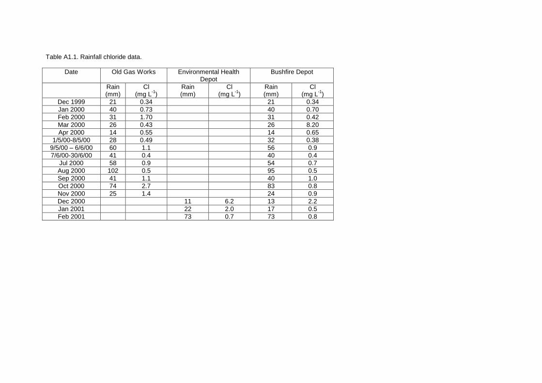
Table A1.1. Rainfall chloride data.

Date Old Gas Works Environmental Health Depot

Bushfire Depot

Rain (mm)

Cl (mg L-1)

Rain (mm)

Cl (mg L-1)

Rain (mm)

Cl (mg L-1)

Dec 1999 21 0.34 21 0.34 Jan 2000 40 0.73 40 0.70 Feb 2000 31 1.70 31 0.42 Mar 2000 26 0.43 26 8.20 Apr 2000 14 0.55 14 0.65

1/5/00-8/5/00 28 0.49 32 0.38 9/5/00 – 6/6/00 60 1.1 56 0.9 7/6/00-30/6/00 41 0.4 40 0.4

Jul 2000 58 0.9 54 0.7 Aug 2000 102 0.5 95 0.5 Sep 2000 41 1.1 40 1.0 Oct 2000 74 2.7 83 0.8 Nov 2000 25 1.4 24 0.9 Dec 2000 11 6.2 13 2.2 Jan 2001 22 2.0 17 0.5 Feb 2001 73 0.7 73 0.8

Appendix 2: Reticulated water chemistry

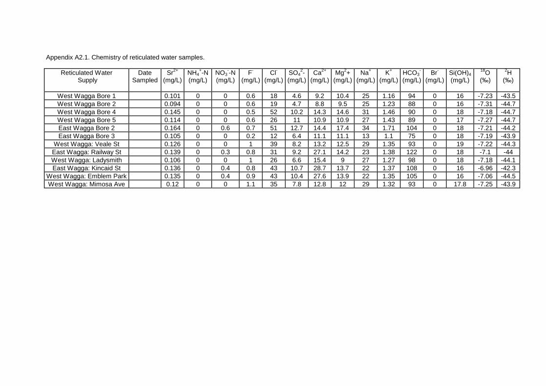
Appendix A2.1. Chemistry of reticulated water samples.

Reticulated Water Supply

Date Sampled

Sr2+ (mg/L)

NH4+-N

(mg/L) NO3

--N (mg/L)

F- (mg/L)

Cl- (mg/L)

SO42-

(mg/L) Ca2+

(mg/L)Mg2+

(mg/L)Na+

(mg/L) K+

(mg/L)HCO3

-

(mg/L) Br-

(mg/L)Si(OH)4 (mg/L)

18O (‰)

2H (‰)

West Wagga Bore 1 0.101 0 0 0.6 18 4.6 9.2 10.4 25 1.16 94 0 16 -7.23 -43.5 West Wagga Bore 2 0.094 0 0 0.6 19 4.7 8.8 9.5 25 1.23 88 0 16 -7.31 -44.7 West Wagga Bore 4 0.145 0 0 0.5 52 10.2 14.3 14.6 31 1.46 90 0 18 -7.18 -44.7 West Wagga Bore 5 0.114 0 0 0.6 26 11 10.9 10.9 27 1.43 89 0 17 -7.27 -44.7 East Wagga Bore 2 0.164 0 0.6 0.7 51 12.7 14.4 17.4 34 1.71 104 0 18 -7.21 -44.2 East Wagga Bore 3 0.105 0 0 0.2 12 6.4 11.1 11.1 13 1.1 75 0 18 -7.19 -43.9

West Wagga: Veale St 0.126 0 0 1 39 8.2 13.2 12.5 29 1.35 93 0 19 -7.22 -44.3 East Wagga: Railway St 0.139 0 0.3 0.8 31 9.2 27.1 14.2 23 1.38 122 0 18 -7.1 -44 West Wagga: Ladysmith 0.106 0 0 1 26 6.6 15.4 9 27 1.27 98 0 18 -7.18 -44.1 East Wagga: Kincaid St 0.136 0 0.4 0.8 43 10.7 28.7 13.7 22 1.37 108 0 16 -6.96 -42.3

West Wagga: Emblem Park 0.135 0 0.4 0.9 43 10.4 27.6 13.9 22 1.35 105 0 16 -7.06 -44.5 West Wagga: Mimosa Ave 0.12 0 0 1.1 35 7.8 12.8 12 29 1.32 93 0 17.8 -7.25 -43.9

Appendix 3: Bore water chemistry

Table A3.1 Bore water chemistry.

Bore Date Sampled

Sr2+ (mg/L)

NH4+-N

(mg/L) NO3

--N(mg/L)

F- (mg/L)

Cl- (mg/L)

SO42-

(mg/L) Ca2+

(mg/L) Mg2+

(mg/L) Na+

(mg/L)K+

(mg/L)HCO3

-

(mg/L) Br-

(mg/L)Si(OH)4 (mg/L)

18O (‰)

2H (‰)

14C (pmc)

13C (‰)

Emblem 1/1 13.1.99 0.922 0 1.3 1.3 592 148 34.9 78.8 336 2.05 250 1.8 5.3 -6.83 -42.7 47.8 -14.6 Emblem 1/2 13.1.99 0.835 0 1.8 1.8 444 126 40.9 67.4 285 2.42 305 1.4 4.6 -6.75 -41.8 37.8 -14.6 Emblem 1/3 13.1.99 0.876 0 0.9 2.3 326 86 33.6 51.4 218 2.98 250 1.1 5.2 -6.96 -43.2 29.8 -14.3 Emblem 2/1 13.1.99 0.883 0 1.8 1.6 513 118 41.6 74 275 2.44 238 1.8 5.2 -7.01 -44 48.1 -14.7 Emblem 2/2 13.1.99 0.944 0.1 1.5 1.7 534 119 47.5 74.4 280 2.86 244 1.7 4.9 -6.93 -43.8 35.5 -14.4 Emblem 2/3 13.1.99 0.923 0 1.2 1.9 517 113 47.9 72.7 264 3.22 232 1.7 5 -6.9 -43.3 29.1 -14.4

4 16.12.99 4.03 0 0.9 1569 178 485 206 393 32.6 597 6.4 24 -5.15 -30.3 5 16.12.99 2.85 0 0.9 1696 200 213 139 884 1.71 726 8.7 19 -5.15 -35.1 95.9 -12.8 6 16.12.99 6.83 0 1.4 6475 1535 304 508 3221 13.63 1021 27.9 30 -4.98 -32.9 7 16.12.99 10.2 0 1.4 8560 1316 518 709 3228 1.08 520 33.3 23 -4.84 -32.7 9 16.12.99 5.22 0 0.9 3130 172 387 307 1036 10.31 420 15.4 15 -5.35 -34.4 10 16.12.99 6.69 0 1.4 3710 119 578 290 1103 1.61 408 14.6 30 -5.4 -34 11 16.12.99 1.13 5.1 0.9 501 38.9 71 55 430 1.2 496 1.9 22 -5.24 -32.7 19 16.12.99 0.938 5.3 0.9 478 287 86 48 634 10.98 750 0 32 -5.43 -33.9 91.5 -13.9 34 13.1.99 5.34 0 0 0.5 1958 1023 294 286 974 16.8 470 8.7 5.5 86.9 -13.7 37 13.1.99 1.28 0.1 0 0.7 852 215 102 115 332 4.3 256 3.6 5.3 -6.4 -40.6 46.9 -15.9 38 13.1.99 0.28 0.1 10.4 2.1 470 154 11.7 19.8 844 3.6 1074 2.6 10.4 90.3 -14.3 42 16.12.99 2.56 0 0.9 1344 325 161 143 730 2.18 516 4.8 15 -5.08 -33.6 92.1 -13.5 43 13.1.99 0.563 0.1 7.4 0.3 3288 478 535 265 1120 6.08 226 11.3 14.3 90.1 -16.5 44 16.12.99 2.92 0 0.9 2355 688 193 166 1204 18.9 299 11.9 22 -5.61 -32.5 47 18.5.99 1.59 0 4.6 3 1007 140.3 108.6 82.2 622 6.2 -5.06 -27.3 30.6.99 -5.47 -33.5 16.12.99 3.4 0 0.9 2329 245 246 196 897 7.33 220 12.2 25 -5.65 -31.3

59 17.5.99 1.42 0 0 3 853 223 62.9 91.3 567 16.11 -5.1 -30.5 67 18.5.99 1.17 0 0 4 736 193.5 49.4 75.4 715 2.14 12.7.99 -5.57 -36.1

68 3.6.99 0.815 0 0 3 1541 850.3 44.5 51.2 1461 2.95 -5.49 -34.5 69 18.5.99 1.22 0 1.6 2 487 49.2 85.6 77 206 0.74 -5.76 -36 90 13.1.99 6.08 0 0 1.8 3832 1134 135 502 1692 4.05 659 16 7.8 -5.58 -37.1

Appendix 4: Bedrock fracture characteristics

Fracture orientations in the Ordivician metasediments were mapped at three outcrop locations:

the model railroad tunnel, Pomingalarna Park and Southern Roadbase quarry. Details of

orientations of all measured fractures are given in Table A4.1.

A4.1. Model Railroad Tunnel

The outcrop at this location consisted of two sides of a trench dug to accommodate a tunnel

approximately 30 m long by 2 m high. The primary feature in the outcrop was iron staining

on the fracture planes. A few small quartz veins occurred in the outcrop, but they appear to be

very minor. In the outcrop, the density of bedding plane fractures appears to dominate over

shear fractures. This may be a weathering feature and not a characteristic of the aquifer at

depth.

Although the outcrop was fairly substantial, it had a number of problems in making it a

valuable correlation with regional fracture properties of the metasediments. The outcrop had

creep occurring on the upper portions of the outcrop and near the tunnel itself. Some of the

outcrop has been artificially replaced for aesthetic reasons, but this can usually be recognised

by the mortar used to hold the “new” outcrop in place. When comparing the bedding

orientation at this outcrop with the 1:100,000 map of the area (Raymond, 1993), it appears to

be strongly influenced by the proximity to the Silurian granites, rotating the bedding

counterclockwise relative to the general trend of the bedding.

The bedding plane fractures at the outcrop had an average strike and dip of 113/81 (Fig. A4.1,

Table A4.1). The shear plane fractures had an average of 189/58 and 23/61. Further work

may separate these fractures into three sets (one vertical, and two near 60°).

74

(b)(a)

Figure A4.1. Fracture orientation data of Ordivician metasediments mapped from exposures in the Model Railroad tunnel. (a) Contour diagram of poles to fracture planes. Contours near edges of the diagram indicate steeply dipping fractures. Horizontal fractures would lie in the centre of the circle. (b) Rose diagram of fracture orientations. Solid lines indicate average orientation of fracture plane. Shaded areas indicate the full range of variation in the data sets. Individual measurements used to construct these plots are given in Table A4.1.

A4.2. Pomingalarna Park

The outcrop at this location consisted of a three-sided quarry dug into a rise. It was water-

filled at the time of this investigation. The walls were approximately 3 m high and 30-50 m in

length. The fractures at this outcrop were also stained with iron, but appeared to be

weathering differently, which suggests a potential difference in the fracture skin composition.

A few small quartz veins occurred in the outcrop, but they appear to be minor. Although the

outcrop was fairly substantial, it suffered from the same weathering properties that the other

outcrops had with creep occurring on the upper portions of the outcrop.

The bedding plane fractures at the outcrop had an average strike and dip of 340/85 (Fig.

A4.2). The shear plane fractures had an average of 223/62 and 57/73. Further work may

separate these fractures into three sets (one vertical, and two near 60°).

75

(b)(a)

Figure A4.2. Fracture orientation data of Ordivician metasediments mapped from exposures in Pomingalarna Park. (a) Contour diagram of poles to fracture planes. (b) Rose diagram of fracture orientations. Individual measurements used to construct these plots are given in Table A4.1.

A4.3. Southern Roadbase Quarry

The outcrop at this location consisted of a large quarry excavating a hill. The quarry had a

depth of approximately 50 m and provided the highest quality and largest extent of outcrop.

The fractures at this outcrop were also stained with iron. The quarry provided exposure of at

least one large (3 m) bedding parallel anticline. Although the outcrop was fairly substantial, it

suffered from the same weathering properties as other outcrops with creep occurring on the

upper portions. The quarry also had a large amount of talus at the base of the outcrops

limiting the ability to conduct scanlines. However, this would provide the best site for this

technique of the available locations.

The bedding plane fractures at the outcrop had an average strike and dip of 330/88 (Fig. A4.3,

A4.4). The shear plane fractures had an average of 216/35 and 53/60. Further work will be

required to determine the cause of the variability in shear planes between the three outcrops.

The quarry also provided some qualitative information on the fracture properties of the

formation. The shear set striking 53° had a much higher density (smaller spacing) than the set

striking 216°. The shear set striking 216° had much more damage along the fracture planes,

sometimes represented as centimetre-scale zones of damage. The quarry owner also provided

information that when the quarry was water filled, the water was transmitted along the

bedding plane fractures and caused a seep on the north-northwest side of the hill.

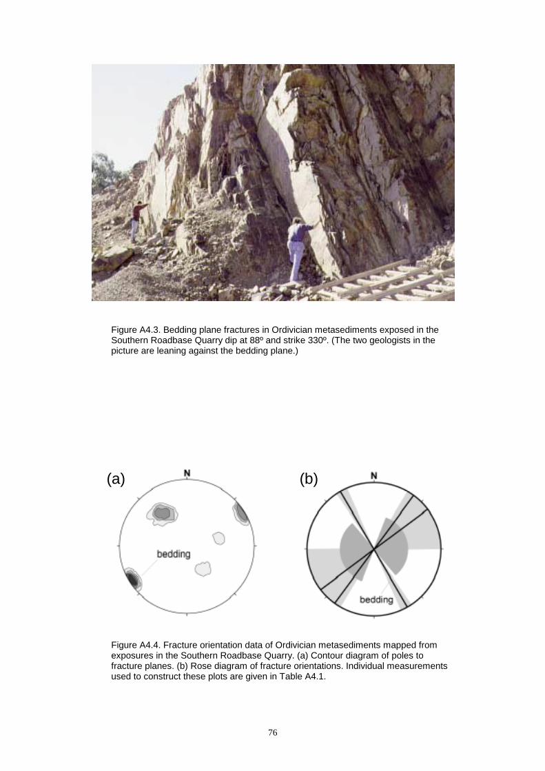
76

Figure A4.3. Bedding plane fractures in Ordivician metasediments exposed in the Southern Roadbase Quarry dip at 88º and strike 330º. (The two geologists in the picture are leaning against the bedding plane.)

(b)(a)

Figure A4.4. Fracture orientation data of Ordivician metasediments mapped from exposures in the Southern Roadbase Quarry. (a) Contour diagram of poles to fracture planes. (b) Rose diagram of fracture orientations. Individual measurements used to construct these plots are given in Table A4.1.

Table A4.1. Outcrop orientation measurements from Ordivician metasediments.

Model Railroad Tunnel Pomingalarna Park Southern Roadbase Quarry

Bedding Shear 1 Shear 2 Bedding Shear 1 Shear 2 Bedding Shear 1 Shear 2 Strike Dip Strike Dip Strike Dip Strike Dip Strike Dip Strike Dip Strike Dip Strike Dip Strike Dip

95 90 148 31 325 45 333 87 202 53 42 75 326 90 164 48 30 4999 79 153 61 329 25 336 89 203 82 43 71 326 90 169 42 35 65107 80 169 69 338 28 339 84 210 87 49 84 328 85 201 25 38 85115 80 174 77 351 31 342 81 252 63 49 71 332 89 203 75 41 61116 74 177 80 356 43 344 87 273 36 57 89 332 82 229 40 48 67117 79 179 88 1 60 345 81 69 64 336 79 233 38 48 55119 83 181 89 2 45 70 80 148 87 255 31 50 53122 82 183 29 10 84 83 55 148 86 270 82 51 86123 81 189 59 10 63 155 85 283 70 52 46

199 63 21 71 295 47 52 59 203 56 23 87 318 51 54 80 205 66 26 86 320 50 55 58 213 70 27 86 55 56 218 73 33 86 56 61 230 16 39 64 58 52 247 31 62 84 59 65 77 82 60 49 79 88 68 47 69 40 90 77

Averages 113 81 189 58 23 61 340 85 223 62 57 73 330 88 216 35 53 60