1

Simulating turbulent swirling flow in a gas cyclone: a comparison of various modelling

approaches

G. Gronald1 & J.J. Derksen2

1AE&E Austria GmbH&CoKG, Waagner-Biro-Platz 1, 8074 Raaba/Graz, Austria

2Chemical & Materials Engineering, University of Alberta, Edmonton, Alberta, T6G 2G6 Canada

Submitted to Powder Technology, April 2010

Accepted: September 2010

Abstract

The single phase flow field of a gas cyclone has been simulated with a finite volume RANS model and

two LES approaches – one with finite volume and one with lattice-Boltzmann discretization. In order

to evaluate their quality, the modelling results have been compared with LDA velocity measurements

taken from the literature. Since the steady-state RANS simulation did not result in a converged

solution, an unsteady RANS simulation was performed and used for further evaluations. The peak-

levels of the time-averaged tangential velocity are well predicted by the two LES approaches whereas

the RANS-based simulation under-predicts them. For the mean axial velocity, all models perform

equally well. Velocity fluctuation levels (in terms of the root-mean-square values of the tangential and

axial velocity components) are much better predicted by the large eddy simulations as compared to the

RANS simulation. This relates to vortex core precession, the frequency of which was analysed for the

two LES approaches. It agreed within 10% with experimentally obtained data. In conclusion, unsteady

RANS-based simulations on a relatively coarse grid can provide reasonable and industrially relevant

results with limited computational effort, whereas simulations that accurately capture the flow physics

require a large eddy approach on fine grids.

Keywords: gas cyclone, computational fluid dynamics, turbulence, swirling flow

2

Introduction

Cyclones are widely used devices to separate a dispersed phase (e.g. particles or droplets) from a

continuous phase (e.g. gaseous or liquid) with the phases having different densities. The working

principle of a cyclone is based on a swirl flow that induces a net centrifugal force that is linear in the

density difference. In this paper we focus on gas cyclones that are used to clean gas streams

contaminated with solid particles or liquid drops. Even though the invention of Morse [1] is more than

one hundred years old, its geometry has not been changed very much although modern manufacturing

techniques would allow almost every conceivable shape. Especially the simple design consisting of a

cylindrical and conical body, a cover plate and in- and outlets leads to its advantages which are low

manufacturing and maintenance costs, operation safety, and potential for separation at elevated

temperatures. Initially mainly applied as final-stage gas cleaning devices, more stringent

environmental restrictions pushed the cyclone towards the middle of processes in applications such as

fluidized bed combustion, fluid catalytic cracking, cement production, and mining.

Although cyclones are characterized by simple construction, their flow fields and the separation

process are very complex. The gas motion usually is highly turbulent and fundamentally three-

dimensional. Due to swirl, the turbulence is strongly anisotropic, and the swirling motion possesses an

inherent instability: the core of the vortex precesses around the geometrical axis of the cyclone adding

a semi-coherent motion to the turbulent fluctuations.

According to a widely accepted separation theory (Muschelknautz and Brunner [2]), the

centrifugal force induced by the spiraling motion of the continuous phase pulls the dispersed phase

against the drag force due to an inward radial fluid flow outwards to the wall; at the wall a boundary

layer conveys the separated phase towards the outlet (e.g. dust bin or drop tube). Also secondary

separation mechanisms have been reported in the literature. Hoffmann et al. [3, 4] postulate that a

certain amount of the entering particles are separated during the first circulation in the cyclone without

classification. The mass loading effect (see Hoffmann and Stein [5]) is thought to help separate fine

particles by shielding. Ter Linden [6] explains a better separation at higher loadings by small particles

being swept towards the wall by big particles. Agglomeration effects due to van der Waals or

3

electrostatic forces are often used to explain the separation of submicron particles that according to

common theory would not be collected (Stairmand [7]; Abrahamson et al. [8]). Despite the above

mentioned effects, the predominating separation mechanism is the centrifugal force induced by the

swirling gas flow.

As for other process equipment, cyclone performance parameters like separation efficiency, cut

size, and pressure drop need to be estimated during process design. Generally speaking, these

parameters can be predicted with semi empirical models that have been developed over the years. In

Europe, cyclone performance parameters are often calculated according to the model of

Muschelknautz and Brunner [2] which considers a force balance of drag and centrifugal force as

suggested by Barth [9]. In America, the Leith and Licht model (see Leith and Licht [10]) is frequently

used which also considers a force balance. Dietz [11] introduced a model based on differential mass

balances which are formulated for three zones in the cyclone. Mothes and Löffler [12] as well as

Lorenz [13] extended the Dietz model with one additional zone each. All these models include the

main cyclone parameters (e.g. body diameter D, height H, length S and diameter Dx of the vortex

finder), but they are not able to reflect every geometrical detail, have limited applicability, and limited

accuracy.

In principle, numerical models can overcome this problem. With modern simulation techniques,

it is possible to represent every detail of the separator’s geometry in a full-scale model. From a

computational point of view it is very challenging to describe all features accurately; this capability of

Computational Fluid Dynamics (CFD) distinguishes numerical methods from semi-empirical models.

The challenges are that besides a comprehensive flow model many effects like phase interaction

(Derksen et al. [14]) and inter-particle collisions including agglomeration (Sommerfeld and Ho [15])

and breakage should be taken into account in order to get reliable results in terms of process

performance. Steadily increasing computer power and simultaneously declining computer hardware

costs enable the industrial application of high-performance computational methods. Pre-processing

(e.g. generation of the numerical grid), simulation, and post-processing (data analysis) can be carried

out within hours to days, depending on the numerical models used, their level of detail, and the

4

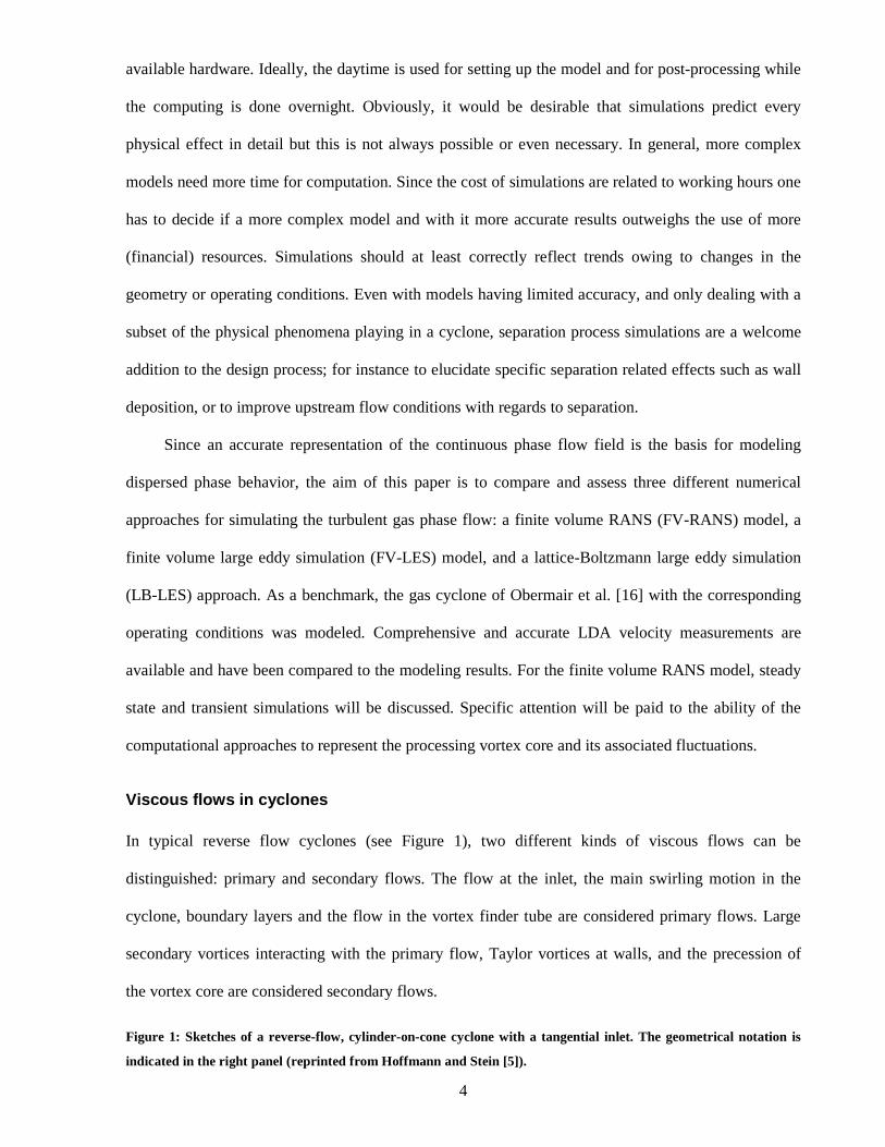
available hardware. Ideally, the daytime is used for setting up the model and for post-processing while

the computing is done overnight. Obviously, it would be desirable that simulations predict every

physical effect in detail but this is not always possible or even necessary. In general, more complex

models need more time for computation. Since the cost of simulations are related to working hours one

has to decide if a more complex model and with it more accurate results outweighs the use of more

(financial) resources. Simulations should at least correctly reflect trends owing to changes in the

geometry or operating conditions. Even with models having limited accuracy, and only dealing with a

subset of the physical phenomena playing in a cyclone, separation process simulations are a welcome

addition to the design process; for instance to elucidate specific separation related effects such as wall

deposition, or to improve upstream flow conditions with regards to separation.

Since an accurate representation of the continuous phase flow field is the basis for modeling

dispersed phase behavior, the aim of this paper is to compare and assess three different numerical

approaches for simulating the turbulent gas phase flow: a finite volume RANS (FV-RANS) model, a

finite volume large eddy simulation (FV-LES) model, and a lattice-Boltzmann large eddy simulation

(LB-LES) approach. As a benchmark, the gas cyclone of Obermair et al. [16] with the corresponding

operating conditions was modeled. Comprehensive and accurate LDA velocity measurements are

available and have been compared to the modeling results. For the finite volume RANS model, steady

state and transient simulations will be discussed. Specific attention will be paid to the ability of the

computational approaches to represent the processing vortex core and its associated fluctuations.

Viscous flows in cyclones

In typical reverse flow cyclones (see Figure 1), two different kinds of viscous flows can be

distinguished: primary and secondary flows. The flow at the inlet, the main swirling motion in the

cyclone, boundary layers and the flow in the vortex finder tube are considered primary flows. Large

secondary vortices interacting with the primary flow, Taylor vortices at walls, and the precession of

the vortex core are considered secondary flows.

Figure 1: Sketches of a reverse-flow, cylinder-on-cone cyclone with a tangential inlet. The geometrical notation is

indicated in the right panel (reprinted from Hoffmann and Stein [5]).

5

After entering the cyclone at the inlet, the main flow is built up. This is a highly three-

dimensional and turbulent flow, whose circumferential component is about three times as high as the

superficial inlet velocity. This is larger than the typical axial velocity (which is of the same order as the

inlet velocity), and one order of magnitude larger than the velocity in radial direction. Circumferential

velocity profiles (i.e. circumferential velocity as a function of radial position) do not change much over

the height of the cyclone (see Peng et al. [17]) and can be captured with the following two-parameter

model (Shepherd and Lapple [18])

tannU r c⋅ = (1)

with c and n model parameters. Close to the centerline (see Figure 2), the flow behaves like a forced

vortex ( 1n = − ); the circumferential velocity increases linearly with increasing distance from the

centerline. Approximately at the radius of the vortex finder tube, the maximum tangential velocity is

reached. For larger radii, the profile is akin to a free vortex with the exponent n having values in the

range 0.5-0.6 (a truly free vortex has 1n = ).

In the near wall region, the flow in axial direction is towards the dust bin and in the core of the

cyclone upwards to the vortex finder tube (see the lower panel of Figure 2). The radial velocity is

considered to be almost constant over the height of the cyclone, except for a strongly inward velocity

right under the vortex finder tube which is often referred to as ‘leap leakage’ (Hoffmann and Stein [5]).

This peak in radial velocity is one of the reasons for non-ideal separation and the typical S-shaped

form of the grade efficiency curve (i.e. separation efficiency versus particle size) of a cyclone.

Velocity profiles will be revisited in much more detail when the simulation results are discussed.

Figure 2: Schematic representation of tangential and axial velocities in a cyclone.

In the vortex finder tube swirl still dominates the flow and wall friction there is responsible for a

major part of the cyclone’s pressure drop. The viscous flow in the boundary layers of the cover plate

and the cone are important because on the one side they carry already separated dispersed matter at the

cyclone’s wall to the outlet (positive effect). On the other side they can cause slip at the cover plate

resulting in non-ideal separation (negative effect, ‘leap leakage’). The reason for this effect is the

6

pressure field in the cyclone which persists throughout the boundary layer to the wall. In contrast, the

tangential velocity decreases in the boundary layer towards zero at the wall (no-slip condition). As a

result, the boundary layer flow is directed to the cyclone’s center line driven by the pressure field.

Apart from the above mentioned primary flows, there exist secondary flows in the cyclone,

which are due to different mechanisms. Taylor vortices are produced by the destabilizing effect of a

centrifugal force close to the concave wall. As well as boundary layer flows, secondary vortices are the

result of the no-slip condition at the wall and the pressure distribution in the cyclone. Another

secondary flow phenomenon is the precessing vortex core (PVC). Many experimental studies have

shown that the point of zero average circumferential velocity is not exactly on the geometrical

centreline of the cyclone; it is laterally displaced with the lateral displacement being a function of the

axial position. In addition the vortex core precesses around the centreline, adding velocity fluctuations

that are of the same order of magnitude as the turbulent fluctuations (Hoekstra et al. [19]). The cause

of the PVC can be found (according to Hoekstra et al. [20]) in hydrodynamic instabilities of the flow.

Depending on the operating conditions and cyclone geometry, the frequency of the precession was

measured to be between 13 Hz and 400 Hz (see Smith [21], Yzdabadi et al. [22], Hoekstra et al. [23]).

Over a wide range of flow rates it scales linearly with the flow rate giving rise to a constant Strouhal

number. Derksen and van den Akker [24] simulated the precessing vortex core with a large eddy

simulation with lattice-Boltzmann discretisation. They found good agreement (within 10%) between

measured and simulated frequencies.

Boysan, Ayers and Swithenbank [25] presented results of CFD simulations of a cyclone with a

finite difference method and an algebraic turbulence model. They could successfully reproduce the

experimentally observed flow field. Additionally they found, that turbulence closures based on the

assumption of isotropy (as e.g. in the k-ε model) are incapable of correctly resolving strongly swirling

flows. Minier, Simonin and Gabillard [26] also reported on shortcomings of the k-ε model concerning

the characteristic size of turbulent eddies in cyclone separators. Meier and Mori [27] simulated the gas

flow in a cyclone in two dimensions with an isotropic k-ε model and an anisotropic model being a

combination of the k-ε model and the generalized mixture length model of Prandtl. For evaluations

7

they compared the results with experimental data. Their main conclusion was that only anisotropic

turbulence models can predict the swirling flows in a cyclone successfully. Hoekstra et al. [20]

reported on reasonable agreement with experimental data, when the anisotropic Reynolds stress

turbulence model was applied. With increasing computational power, large eddy simulations and with

it transient aspects become available for cyclone simulations. In this computationally more expensive

technique, the larger eddies which are responsible for the anisotropy are simulated directly while

smaller eddies are accounted for with a relatively simple subgrid-scale model. Slack et al. [28] showed

good agreement between LDA measurements and LES simulations. Derksen et al. [14] also achieved a

very good agreement between measurements and LES simulations.

It is important to note here that simulation results should not only be assessed in terms of the

average velocities; also velocity fluctuation levels are very important. Accurate prediction of velocity

fluctuation levels is needed for getting the separation performance right; in fact particle separation can

be viewed as a competition between centrifugal forces that bring particles to the cyclone wall, and

turbulent dispersion that spreads them over the cyclone volume with the chance they get caught in the

stream leaving through the vortex finder.

Cyclone geometry and LDA data set

Obermair et al. [16] measured the flow field in the lower part of three different dust outlet geometries

of a laboratory-scale cyclone using a two dimensional laser Doppler anemometry (LDA) system. The

three geometries have (1) a simple dust bin, (2) a dust bin with apex cone, and (3) a 500 mm long drop

tube with a simple dust bin attached to it. The results of these measurements are mean axial and mean

tangential velocities as well as their respective root mean square (rms) values in a vertical plane in the

cyclone. In a number of cross sections, the radial velocity has also been measured. In order to

determine the quality of the present modeling results, the flow field in the cyclone with drop tube and

dust bin (labeled as geometry C in Obermair et al. [16]) has been simulated and the corresponding

measurement results were taken as benchmark data.

Figure 3 shows a sketch of the cyclone geometry including the origin of the coordinate system

8

that will be used throughout this paper. For optical access, Obermair et al. equipped the cyclone with

rectangular glass windows and measured with the LDA system in a backscatter mode. During the

measurements, the cyclone was operated with a constant volumetric flow rate of air of 800 Am³/h at

laboratory conditions summarized in Table 1. The Reynolds number (Re) based on the cyclone body

diameter D and the superficial inlet velocity Uin is Re=282000. As seeding for the LDA experiments,

oil droplets (Diethylhexylsebacat) with a density of 912 kg/m³ and a mean diameter of 0.25 µm were

used; they very well followed the flow. As an indication: they could hardly be centrifuged out, even at

inlet velocities that were much higher than used in the LDA experiments. Using this experimental

configuration, the average velocities were measured with an error smaller than 1%. There is a

measurement location every 5 mm in the core region, and every 10 mm outside the core region (see

Figure 4). The main measurement plane was parallel to the tangential inlet of the cyclone (the z-x-

plane). Figure 5 shows measurement results in this plane for the mean axial and mean tangential

velocity as presented earlier by Obermair et al [16]. It can be clearly seen, that the vortex core wraps

around the centerline of the cyclone. In Figure 5 several levels are marked which are later used for

detailed comparisons with the modeling results.

Figure 3: Definition of the cyclone geometry including the coordinate system.

Table 1: Cyclone operating conditions at LDA measurements (Obermair et al. [16]).

Figure 4: Location of velocity measurements in the benchmark (Obermair et al. [16]) experiment. Measurements

have been performed in the blue and red marked planes.

Figure 5: LDA measurement results of Obermair et al. [16]: mean axial and mean absolute tangential velocity in

the cyclone. For reference: the superficial inlet velocity amounts to Uin=12.68 m/s. The dashed horizontal lines

indicate the axial locations of the velocity profiles we will use for comparing experimental and computational

results.

Computational approaches & turbulence modeling

It is the aim of the present work to compare the results achieved with three different CFD approaches.

9

These approaches are not only different regarding the discretization method for approximating the

differential equations by a system of algebraic equations but also with respect to turbulence modeling.

Additionally, the size of the numerical grids (in terms of the number of nodes) varies by one order of

magnitude. Finer grids increase accuracy but also require more computational power. All simulations

reported are three-dimensional. The following three approaches have been used:

• finite volume RANS model (FV-RANS)

• finite volume large eddy simulation (FV-LES)

• lattice Boltzmann large eddy simulation (LB-LES)

Among many known discretisation schemes, the finite volume method is one of the most popular

methods since it is relatively simple to understand and to implement in computer code. The method

can accommodate any type of grid which makes it suitable for complex geometries and thus use in

industry (Ferziger and Peric [29]). Hence, many commercial CFD codes apply this discretization

methodology. The advantages of the lattice Boltzmann method are its computational efficiency and

locality of operations leading to inherent parallelism.

Steady-state and transient FV-RANS

The simulations with the steady state and transient FV-RANS approach have been performed with the

commercial CFD code Fluent 6.3.26. By using a modern software package, simulations of the flow in

cyclones can be done with acceptable efforts, assuming one observes the recommendations found in

the literature. Some details about the model and the numerical solution technique are summarized in

Table 2. The flow is assumed to be incompressible and isothermal. Turbulence is accounted for with

the Reynolds stress turbulence model because of the high anisotropy of the swirling flow. On wall

boundaries the standard wall function is applied since a full resolution of the boundary layer is not

necessary. For high-quality results higher order schemes for numerical discretizations have to be used.

Hence, in the FV-RANS model the QUICK scheme was applied for all equations. In Fluent the Quick

scheme is based on a weighted average of second-order-upwind and central interpolations of the

variable. It is only available for quadrilateral and hexahedral cells and, thus, only these types were

used. Detailed information on the models in Fluent can be found in the Fluent User’s Guide [30]

Table 2: Simulation settings in the FV-RANS model

Finite volume LES

With increasing computational power, LES methods become applicable to industrial flows. Compared

to the RANS approach, turbulence modelling is less speculative. In LES simulations, the largest eddies

are directly resolved by the grid and for smaller eddies (subgrid scales eddies) a turbulence model

10

(subgrid scale model) is used. Since the subgrid scale models are based on the universal behaviour of

turbulence in and beyond the inertial subrange, and since the grid determines which eddies are

resolved and which have to be modelled, substantially finer grids are necessary in LES simulations.

In the present work Fluent 6.3.26 has been adopted for the simulation with the finite volume LES

approach. The same methodology for grid generation has been applied but in comparison to the FV-

RANS model a finer grid has been created (roughly 5 million cells, as compared to 1.3 million in the

RANS). For subgrid scale modelling the Smagorinsky-Lilly model has been applied with the default

value of the Smagorinsky constant 0.1Sc = . Stochastic velocity fluctuations have been neglected at the

inlet boundary since the results of previous cyclone simulations did not show a dependency on this

condition. Owing to the size of the grid in the near wall regions, Fluent applies the law-of-the-wall in

the FV-LES because the centre of the first near wall cell is already in turbulent regions. The bounded

central differencing scheme has been applied for spatial discretization. It is of second accuracy and the

default scheme for large eddy simulations in Fluent. In Table 3 the simulation settings for the FV-LES

model have been summarized. Detailed information on the models in Fluent can be found in the Fluent

User’s Guide [30].

Table 2: Simulation settings in the FV-LES model Lattice-Boltzmann-based LES

As an alternative for finite volume discretization of the Navier-Stokes equations, lattice-Boltzmann

methods offer a few advantageous features. A lattice-Boltzmann fluid consists of fluid parcels residing

on a uniform, cubic lattice. The parcels move from lattice site to lattice site thereby colliding with

parcels arriving at the same site coming from other directions. The collisions give rise to viscous flow

behavior. Rigorous derivations (see e.g. Succi [31]) show that – with the right lattice topology and

collision rules – this discrete particles system mimics the Navier-Stokes equations. The assets of the

method are its inherent parallelism, and its computational efficiency (in terms of number of operations

per lattice site and time step), both assets not being hampered by geometrical complexity. In previous

work on large-eddy flow simulations in process equipment (e.g. Derksen and Van den Akker [32]) and

specifically in swirling flow (Derksen and Van den Akker [24]; Derksen [33]) the potential of this

11

approach has been demonstrated when coupled to a standard Smagorinsky subgrid-scale model.

The uniform, cubic grid to represent the cyclone geometry has a spacing of 200

D∆ = . As in

previous work, no-slip conditions at non-flat surfaces have been imposed by an immersed boundary

method (Derksen and Van den Akker [32]). In the LB-LES simulation the Smagorinsky constant was

set to 0.1Sc = .

Results and discussion

In the following, the results of the three different modeling approaches are compared among each other

and with the LDA velocity measurements of Obermair et al. [16]. The locations of the six radial

profiles which are mainly used for this evaluation are shown in Figure 5. Starting in the cyclone’s

cone, the profiles are almost evenly distributed along z-axis until in the dust bin.

Steady-state RANS simulations

Figure 6: Development of average tangential velocity profiles at three axial locations with the iteration number in a

steady state RANS simulation.

Figure 7: Development of average axial velocity profiles at three axial locations with the iteration number in a

steady state RANS simulation.

Figure 8: Development of the tangential velocity in a certain control volume (located at x=0.188D, y=0, z=1.875D)

with the iteration number.

The first results relate to problems we encountered when attempting a steady-state, RANS-based

simulation. In addition to the relatively poor agreement of the predicted profiles of tangential and axial

velocity (as shown in Figure 6 and 7) the solution does not converge. The profiles keep changing and

the solution enters a marginally stable state with periodic fluctuations as a function of the iteration

number (see Figure 8). These problems most likely relate to the physics of the flow that (as indicated

above and confirmed by the LDA experimental results) develops a precessing vortex core. This quasi-

periodic instability cannot be captured by the Reynolds stress model combined with a steady-state

approach. In what follows, we only will be comparing unsteady RANS results with the LDA data and

the two LES-based simulations.

12

Mean velocity For determining time-averaged velocity profiles, the flow first needs to fully develop to a quasi steady

state. This is monitored by keeping track of the tangential velocity in a number of points in the cyclone

and observe when these turbulent signals settle in quasi steady state. After that we average over a long

enough time window to reach statistical convergence of the mean and mean-square velocity values.

In the FV-RANS simulation we start with a zero-flow field and a steady state model. Depending

on the values of the under relaxation factors, the flow field in the cyclone is developed after about

5000 iterations. At this stage the monitors oscillate around a mean value as we have shown above.

Then we switch to the transient model and after calculating a number of 200 initial time steps

(corresponding to 0.1 s) we start the averaging procedure over a time window of 1 s.

In the FV-LES a similar procedure is followed. In a first step, the solution from the steady state

RANS model is interpolated on the grid of the FV-LES simulation in order to save computer time.

Then the large-eddy simulation is started by calculating a number of time steps. After about 0.1 s, the

residues of the initialization have completely vanished and the flow in the FV-LES is developed. The

averaging procedure is started and again a time window of about 1 s is used.

In the LB-LES simulations the development towards steady state is facilitated by beginning the

simulations on a relatively coarse grid (100

D∆ = instead of 200

D∆ = ). On the coarse grid we start with

a zero-flow field. It then takes typically 75in

D

U for the flow to develop. We then transfer the flow

solution to the fine grid, let that simulation develop and then start the averaging procedure over a time

window of 50in

D

U which corresponds to 1.6 s in real time.

Profiles of simulated and measured mean tangential velocities can be found in Figure 9 in

dimensionless form. The experimentally determined profiles are generally captured well by the three

simulation methods. The peak tangential velocities, as well as the widths of the vortex cores (loosely

defined as the radial distance between the tangential velocity extremes) agree well. The tangential

profiles undergo an interesting development in the axial direction. Moving downward in the drop tube,

13

the profiles clearly get steeper. This is specifically well captured with the FV-LES approach. The

RANS simulations generally predict a too wide vortex core. The LB-LES has some trouble in

capturing the maximum tangential velocities; it underpredicts them slightly.

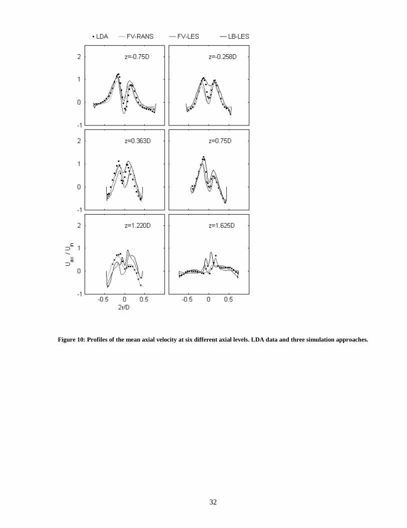
Profiles of the mean axial velocity are shown in Figure 10. In contrast to the mean tangential

velocity, there is no numerical model which is superior. All three models describe the upper four (“M-

shaped”) profiles qualitatively well. Interestingly the asymmetry of the profiles (most strongly at

0.75z D= ) is well represented in the simulations. The agreement with experimental data is less good

compared to the tangential velocity profiles, with poor agreement for the lower two locations. The

detailed and pronounced shape of the axial velocity profiles is due to the details of the axial pressure

gradients that depend on the (axial development) of the tangential velocity. Where the tangential

velocity is to a large extent dictated by the cyclone geometry, the axial velocity is in a complex manner

slaved to the tangential velocity making it harder to predict.

Simulated average radial velocity as a function of the axial (z) coordinate at the radius of the

vortex finder tube ( 0.3752

Dr = ) are given in Figure 11. The two LES profiles are similar, both

showing the strong inward flow just below the vortex finder entrance. Along the rest of the z-axis the

radial velocities are relatively weak. As we will show below, velocity fluctuation levels are at least as

high as mean radial velocities so that the (solid particle) separation process in a cyclone is more than a

competition between outward centrifugal force and inward radial drag (as e.g. in the model due to

Muschelknautz et al. [34]); turbulent dispersion keeping the particles from being separated needs to be

incorporated in the separation models. In Figure 12, there are profiles of the mean radial velocity at

0.32

Dr = depicted, along with a limited set of experimental points. At this (compared to Figure 11)

more inner position, the radial velocity profiles are more pronounced with absolute mean values up

to0.5 inU . The agreement of the simulations and the experimental data is considered fair; the trends as

observed in the experiments are captured by the three simulation approaches. It can also be concluded

from the measurements, that the radial velocity is not constant along the cyclones height as often

assumed in separation models.

14

Figure 9: Profiles of the mean tangential velocity at six different axial levels. LDA data and three simulation

approaches.

Figure 10: Profiles of the mean axial velocity at six different axial levels. LDA data and three simulation approaches.

Figure 11: Profiles of the mean radial velocity as a function of z at the radius of the vortex finder tube (2r/D=0.375)

for the two large-eddy simulations and the unsteady FV-RANS. The angle φφφφ has been defined in Figure 3. There is

one LDA data point at φφφφ=270°, z=0.

Figure 12: Profiles of the mean radial velocity as a function of z at 2r/D=0.3, the three simulations and (dots) LDA

experiments. The angle φφφφ has been defined in Figure 3.

Velocity fluctuation levels As discussed above, velocity fluctuation levels and associated turbulent dispersion are as important for

the separation process as the mean velocities; the former promote spreading of the dispersed phase, the

latter determine the centrifugal force (tangential velocity), and the average residence time in the

cyclone.

Root-Mean-Square (RMS) values of the tangential velocity are shown in Figure 13. It shows

radial profiles at six axial locations. The measurements show peaked curves: relatively low RMS

values in the outer region and high fluctuation levels in the center region. The latter are due to the

precessing vortex core: Since the vortex moves relative to a fixed observer, this observer samples

various locations in the instantaneous circumferential velocity profile. Near the center the gradients in

this profile are very large giving rise to high fluctuation levels.

In this respect, the LES’s distinguish themselves from the RANS-based simulations. The former

are able to capture the RMS levels as induced by the PVC, the latter to a much lesser extent. The

results of the two LES’s are quite different in the dust bin, with the LB-LES giving better predictions.

Similar comments as made about the tangential RMS velocities apply to the axial velocity RMS

profiles, see Figure 14: RANS being unable to predict the fluctuations correctly, the two LES’s doing

fairly good jobs.

Figure 13: Profiles of the RMS-values of the tangential velocity at six different axial levels. LDA data and three

simulation approaches.

Figure 14: Profiles of the RMS-values of the axial velocity at six different axial levels. LDA data and three

simulation approaches.

Vortex velocity

15

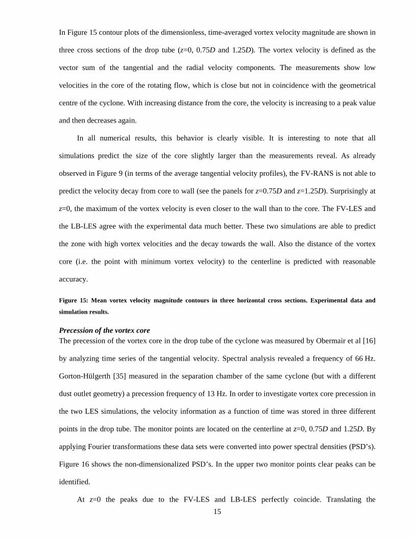
In Figure 15 contour plots of the dimensionless, time-averaged vortex velocity magnitude are shown in

three cross sections of the drop tube (z=0, 0.75D and 1.25D). The vortex velocity is defined as the

vector sum of the tangential and the radial velocity components. The measurements show low

velocities in the core of the rotating flow, which is close but not in coincidence with the geometrical

centre of the cyclone. With increasing distance from the core, the velocity is increasing to a peak value

and then decreases again.

In all numerical results, this behavior is clearly visible. It is interesting to note that all

simulations predict the size of the core slightly larger than the measurements reveal. As already

observed in Figure 9 (in terms of the average tangential velocity profiles), the FV-RANS is not able to

predict the velocity decay from core to wall (see the panels for z=0.75D and z=1.25D). Surprisingly at

z=0, the maximum of the vortex velocity is even closer to the wall than to the core. The FV-LES and

the LB-LES agree with the experimental data much better. These two simulations are able to predict

the zone with high vortex velocities and the decay towards the wall. Also the distance of the vortex

core (i.e. the point with minimum vortex velocity) to the centerline is predicted with reasonable

accuracy.

Figure 15: Mean vortex velocity magnitude contours in three horizontal cross sections. Experimental data and

simulation results.

Precession of the vortex core The precession of the vortex core in the drop tube of the cyclone was measured by Obermair et al [16]

by analyzing time series of the tangential velocity. Spectral analysis revealed a frequency of 66 Hz.

Gorton-Hülgerth [35] measured in the separation chamber of the same cyclone (but with a different

dust outlet geometry) a precession frequency of 13 Hz. In order to investigate vortex core precession in

the two LES simulations, the velocity information as a function of time was stored in three different

points in the drop tube. The monitor points are located on the centerline at z=0, 0.75D and 1.25D. By

applying Fourier transformations these data sets were converted into power spectral densities (PSD’s).

Figure 16 shows the non-dimensionalized PSD’s. In the upper two monitor points clear peaks can be

identified.

At z=0 the peaks due to the FV-LES and LB-LES perfectly coincide. Translating the

16

dimensionless frequency 2.3in

f D

U= as observed there in dimensional terms gives f=73 Hz which is

close to the LDA result of Obermair et al. [16] measured in the dip leg (66 Hz). Then, at z=0.75D, we

observe a shift in the dominant frequency of the LB-LES towards f=60 Hz, whereas the dominant

frequency in the FV-LES stays the same: 73 Hz. Compared to z=0, the periodic signal gets weaker

though. At the end of the drop tube (which is the entrance to the dust bin; z=1.25D), there is no clear

peak and coherent vortex core motion has ceased to exist.

Figure 16: Power Spectral Densities (PSD’s) of the velocity on the centreline at three axial locations. Comparison of

FV-LES and LB-LES results.

Summary and Conclusions

In the present work, high-quality measurements from the literature (Obermair et al. [16]) were

compared to results of three different numerical approaches for modeling the single phase, turbulent

swirling flow in a gas cyclone separator. The three approaches are (1) a simulation based on finite

volume discretization of the Reynolds-averaged Navier-Stokes (RANS) equations coupled to a

Reynolds stress closure model; (2) a finite volume large eddy simulation (LES) and (3) a large eddy

simulation based on lattice Boltzmann discretization of the Navier-Stokes equations. Both LES models

are coupled to a standard Smagorinsky subgrid-scale model. The former two approaches are

implemented in the commercial CFD code Fluent 6.3.26; the lattice-Boltzmann code is a non-

commercial research code.

The steady-state finite volume RANS did not lead to a converged solution; the RANS results as

presented here are based on a transient approach. Several velocity profiles located in the cone, the drop

tube and the dust bin of the cyclone have been extracted from the measurements and used for the

evaluations. The mean tangential velocity which is mainly responsible for the cyclone’s separation

performance is predicted fairly well by both LES models. The FV-RANS approach, however,

underestimates tangential velocity levels. For the mean axial velocity, no significant difference

between all three numerical approaches was observed. The agreement to the experimental data is not

as good as it is for the mean tangential velocity. As often mentioned in the literature, the radial velocity

17

shows a peak just underneath the vortex finder tube entrance which is one reason for non-ideal

separation of cyclones.

Due to the precession of the vortex core, there are high velocity fluctuation levels near the

geometrical centre. They typically are two to three times higher compared to the fluctuations in the

outer region. While the FV-RANS approach is not able to predict this phenomenon correctly, the two

LES simulations are able to describe it. This is encouraging and important given the role of turbulent

dispersion in the separation process. Spectral analysis of velocity time series at three monitor points in

the drop tube revealed the dominant frequencies related to vortex core precession. High up in the drop

tube the two LES models both predict (with remarkable agreement) 73 Hz, whereas the experiment

(Obermair et al. [16]) had 66 Hz. Deeper down in the drop tube the LB-LES sees a shift towards lower

frequencies, in contrast to the FV-LES that keeps showing 73 Hz. The signals get less coherent though

and dominant frequencies cannot be discerned in the dust bin.

As a more general conclusion we show that unsteady RANS-based simulations on a relatively

coarse grid can provide reasonable and industrially relevant results with limited computational effort.

A large-eddy approach and finer grids help in revealing more of the flow physics, at the cost of higher

computational effort.

18

Literature

[1] Morse, O. M., Patent DRP Nr. 39 219, 25.07.1886, Staubsammler, technical report, Knickerbocker

Company, Jackson, USA.

[2] Muschelknautz, E., Brunner, K, Untersuchungen an Zyklonen, Chem. Ing. Techn., 39 (1967), 531-

538.

[3] Hoffmann, A. C., Arends, H., Sie, A., An Experimental Investigation Elucidating the Nature of the

Effect of Solids Loading on Cyclone Performance, Filtration & Separation, 28 (3) (1991), 188-193.

[4] Hoffmann, A. C., van Santen, A., Allen, R. W. K., Clift, R., Effects of geometry and solid loading

on the performance of gas cyclones, Powder Technol, 70 (1992), 83-91.

[5] Hoffmann, A. C., Stein, L. E., Gas Cyclones and Swirl Tubes – Principles, Design and Operation,

Springer, New York, 2002.

[6] Ter Linden, A. Investigations into Cyclone Dust Collectors. Proc. Inst. Mech. Engrs., 160 (1949),

233-239.

[7] Stairmand, C. J., The Design and Performance of Cyclone Separators, Trans. Instn. Chem. Engrs,

29 (1951), 356-383.

[8] Abrahamson, J., Martin, C., Wong, K., The Physical Mechanisms of Dust Collection in a Cyclone.

TransIChemE, 56 (1978), 168-177.

[9] Barth, W., Der Einfluß der Vorgänge in der Grenzschicht auf die Abscheideleistung von

mechanischen Staubabscheidern, Staubbewegungen in der Grenzschicht, VDI Berichte, 6 (1955), 29-

32.

[10] Leith, D., Licht, W. (1972): The Collection Efficiency of Cyclone Type Particle Collectors - a

new Theoretical Approach, Air Pollution and its Control, AIChE Symposium Series, 68 (126), 196-

206.

[11] Dietz, P. W., Collection efficiency of cyclone separators. AIChE J., 27 (6), (1981), 888-891.

[12] Mothes, H., Löffler F., Motion and deposition of particles in cyclones. Ger. Chem. Eng. 27

(1985) 223-233.

19

[13] Lorenz, T., Heißgasentstaubung mit Zyklonen. PhD thesis, Technische Universität Braunschweig,

1994.

[14] Derksen, J.J., van den Akker, H.E.A, Sundaresan, S., Two-Way Coupled Large Eddy Simulations

of the Gas-Solid Flow in Cyclone Separators, AIChE J., 54 (4) (2008), 872-885.

[15] Sommerfeld, M., Ho, C. A., Numerical calculation of particle transport in turbulent wall bounded

flows, Powder Technol., 131 (1) (2003), 1-6.

[16] S. Obermair, J. Woisetschläger, G. Staudinger, Investigation of the flow pattern in different dust

outlet geometries of a gas cyclone by laser Doppler anemometry, Powder Technol., 138 (2003), 239-

251.

[17] Peng, W., Hoffman, A.C., Boot, P., Udding, A., Dries, H.W.A., Ekker, A., Kater, J., Flowpattern

in reverse-flow centrifugal separators, Powder Technol., 127 (2002), 212-222.

[18] Shepherd, C. H., Lapple, C. E., Flow Pattern and Pressure Drop in Cyclone Dust Collectors.

Industrial and Eng. Chemistry, 31 (8) (1939), 972–984.

[19] Hoekstra, A. J., Van Vliet, E., Derksen, J. J., Van Den Akker, H. E. A., Vortex Core Precession in

a Gas Cyclone, Advances in Turbulence VII (1998), 289-292.

[20] Hoekstra, A. J., Derksen, J. J., Van Den Akker, H. E. A., An experimental and numerical study of

turbulent swirling flow in gas cyclones, Chem. Eng. Sci., 54 (1999), 2055-2065.

[21] Smith, J. L., An Experimental Study of the Vortex in the Cyclone Separator, Transactions of the

ASME, 12 (1962), 602-608.

[22] Yazdabadi, P., Griffiths, A., Syred, N., Characterization of the PVC phenomena in the exhaust of

a cyclone dust separator, Experiments in Fluids, 17 (1994), 84-95.

[23] Hoekstra, A. J., Israel, A. T., Derksen, J. J., Van Den Akker, H. E. A., The application of Laser

diagnostics to cyclonic flow with vortex precession, Proceedings of Laser diagnostic to cyclonic flow

with vortex precession. 1 (1998), 4.3.

[24] Derksen, J.J., van den Akker, H.E.A., Simulation of vortex core precession in a reverse-flow

cyclone, AIChE J., 46 (2000), 1317-1331.

[25] Boysan, F., Ayers, W. H., Swithenbank, J., A fundamental mathematical modelling approach to

20

cyclone design, Trans. IChemE., 60 (1982), 222-230.

[26] Minier, J.P., Simonin, O., Gabillard, M., Numerical Modelling of Cyclone Separators, Fluidized

Bed Combustion, ASME, 1991.

[27] Meier H.F., Mori, M., Anisotropic behavior of the Reynolds stress in gas and gas-solid flows in

cyclones, Powder Technol., 101 (1999), 108-119.

[28] Slack, M.D., Prasad, R.O., Bakker, A., Boysan, F., Advances in cyclone modeling using

unstructured grids, Trans. IchemE., 78 (2000), 1098-1104.

[29] Ferziger, J. H., Peric, M., Computational Methods for Fluid Dynamics, third ed., Springer, New

York, 2002.

[30] Fluent 6.0 User’s Guide, Fluent Inc., Centerra Resource Park 10 Cavendish Court Lebanon, NH

03766, 2003.

[31] Succi, S., The lattice Boltzmann equation for fluid dynamics and beyond, Clarendon Press

Oxford, 2001.

[32] Derksen, J.J., van den Akker, H., Large-eddy simulations on the flow driven by a Rushton turbine,

AIChE J. 45 (1999), 209-221.

[33] Derksen, J.J., Simulations of confined turbulent vortex flow, Computers&Fluids, 34 (2005), 301-

318.

[34] Muschelknautz, E., Greif, M., Trefz, T., in: VDI-Wärmeatlas Berechnungsblätter für den

Wärmeübergang, VDI-Verlag, Chapter Lja 1-11 Zyklone zur Abscheidung von Feststoffen aus Gasen.

8th edition.

[35] Gorton-Hülgerth, A., Messung und Berechnung der Geschwindigkeitsfelder und Partikelbahn im

Gaszyklon, PhD. thesis, Graz University of Technology, Austria, 1999.

21

Nomenclature

a inlet height [m]

b inlet width [m]

c constant in Eq. 1 [m1+n /s]

cs Smagorinsky constant [-]

D body diameter of the cyclone [m]

Dx diameter of the vortex finder tube [m]

f frequency [1/s]

H total height of the cyclone [m]

Hc height of the cone [m]

k turbulent kinetic energy [m2/s2]

n exponent in Eq. 1 [-]

psd power spectral density [m2/s2]

r radius [m]

S height of the vortex finder tube [m]

Uin inlet velocity [m/s]

Utan tangential velocity [m/s]

Uax axial veloctiy [m/s]

Ur radial velocity [m/s]

Uv vortex velocity [m/s]

U´tan rms velocity in tangential direction [m/s]

U´ax rms veloctiy in axial direction [m/s]

x, y, z coordinates [m]

∆ grid spacing [m]

ε turbulent dissipation [m2/s3]

φ angle [°]

22

Acknowledgement

The authors would like to thank Prof. Gernot Staudinger and Dr. Stefan Obermair for providing the

LDA data. Support of Dr. Christoph Gutschi in LDA data explorations is gratefully acknowledged.

23

Figure 1: Sketches of a reverse-flow, cylinder-on-cone cyclone with a tangential inlet. The geometrical notation is

indicated in the right panel (reprinted from Hoffmann and Stein, 2002).

24

Figure 2: Schematic representation of tangential and axial velocities in a cyclone.

25

Figure 3: Definition of the cyclone geometry including the coordinate system.

26

Figure 4: Location of velocity measurements in the benchmark (Obermair et al., 2003) experiment. Measurements

have been performed in the blue and red marked planes.

27

mea

n ax

ial v

eloc

ity (

m/s

)

−0.25D 0 0.25D

−0.75D

−0.5D

−0.25D

0

0.25D

0.5D

0.75D

1D

1.25D

1.5D

1.75D

2D

−17

−15.2

−13.4

−11.6

−9.8

−8

−6.2

−4.4

−2.6

−0.8

1

2.8

4.6

6.4

8.2

10

11.8

mea

n ab

solu

te ta

ngen

tial v

eloc

ity (

m/s

)−0.25D 0 0.25D

−0.75D

−0.5D

−0.25D

0

0.25D

0.5D

0.75D

1D

1.25D

1.5D

1.75D

2D

0

2.5

5

7.5

10

12.5

15

17.5

20

22.5

25

27.5

30

32.5

35

37.5

40

z−levels for comparisons of velocity profiles

Figure 5: LDA measurement results of Obermair et al. (2003): mean axial and mean absolute tangential velocity in

the cyclone. For reference: the superficial inlet velocity amounts to Uin=12.68 m/s. The dashed horizontal lines

indicate the axial locations of the velocity profiles we will use for comparing experimental and computational

results.

28

0 0.25 0.5 0.750

1

2

3

2r/D

Uta

n/Uin

z = − 0.75D

0 0.25 0.5 0.75

z = 0.75D

0 0.25 0.5 0.75

z = 1.63D

it# 3500 it# 4500 it# 5500 it# 6500 LDA

Figure 6: Development of average tangential velocity profiles at three axial locations with the iteration number in a

steady state RANS simulation.

29

−1 −0.5 0 0.5 1−1

−0.5

0

0.5

1

1.5

2r/D

Uax

/Uin

z = − 0.75D

−1 −0.5 0 0.5 1

z = 0.75D

−1 −0.5 0 0.5 1

z = 1.63D

it# 3500 it# 4500 it# 5500 it# 6500 LDA

Figure 7: Development of average axial velocity profiles at three axial locations with the iteration number in a

steady state RANS simulation.

30

0 2500 5000 7500 10000 12500 15000−5

0

5

10

15

20

25

30

35

iteration number [−]

tang

entia

l vel

ocity

Uta

n [m/s

]

28

29

30

31

32

Figure 8: Typical development of the tangential velocity in a certain control volume (located at x=0.188D, y=0,

z=1.875D) with the iteration number.

31

−2

0

2

z=−0.75D z=−0.258D

−2

0

2

z=0.363D z=0.75D

−0.5 0 0.5

−2

0

2

z=1.220D

Uta

n / U

in

2r/D−0.5 0 0.5

z=1.625D

LDA FV−RANS FV−LES LB−LES

Figure 9: Profiles of the mean tangential velocity at six different axial levels. LDA data and three simulation

approaches.

32

Figure 10: Profiles of the mean axial velocity at six different axial levels. LDA data and three simulation approaches.

33

2r/D=0.375

−1.5 −1 −0.5 0 0.5

−2

−1.5

−1

−0.5

0

0.5

1

1.5

2

Ur/U

in

z/2D

−1.5 −1 −0.5 0 0.5 −1.5 −1 −0.5 0 0.5 −1.5 −1 −0.5 0 0.5

LDA FV−RANS FV−LES LB−LES

1φ=0°

2φ=90°

3φ=180°

4φ=270°

Figure 11: Profiles of the mean radial velocity as a function of z at the radius of the vortex finder tube (2r/D=0.375)

for the two large-eddy simulations and the unsteady FV-RANS. The angle φφφφ has been defined in Figure 3. There is

one LDA data point at φφφφ=270°, z=0.

34

2r/D = 0.3

−1.5 −1 −0.5 0 0.5

−2

−1.5

−1

−0.5

0

0.5

1

1.5

2

Ur/U

in

z/D

−1.5 −1 −0.5 0 0.5 −1.5 −1 −0.5 0 0.5 −1.5 −1 −0.5 0 0.5

LDA FV−RANS FV−LES LB−LES

1φ=0°

2φ=90°

3φ=180°

4φ=270°

Figure 12: Profiles of the mean radial velocity as a function of z at 2r/D=0.3, the three simulations and (dots) LDA

experiments. The angle φφφφ has been defined in Figure 3.

35

0

0.25

0.5

0.75z=−0.75D z=−0.258D

0

0.25

0.5

0.75z=0.363D z=0.75D

−0.5 0 0.50

0.25

0.5

0.75

U‘ ta

n / U

in

2r/D

z=1.220D

−0.5 0 0.5

z=1.625D

LDA FV−RANS FV−LES LB−LES

Figure 11: Profiles of the RMS-values of the tangential velocity at six different axial levels. LDA data and three

simulation approaches.

36

0

0.25

0.5

0.75z=−0.75D z=−0.258D

0

0.25

0.5

0.75z=0.363D z=0.75D

−0.5 0 0.50

0.25

0.5

0.75

U‘ ax

/ U

in

2r/D

z=1.220D

−0.5 0 0.5

z=1.625D

LDA FV−RANS FV−LES LB−LES

Figure 12: Profiles of the RMS-values of the axial velocity at six different axial levels. LDA data and three

simulation approaches.

37

−0.2−0.1 0 0.1 0.2−0.2

−0.1

0

0.1

0.2

1 1.5 2 2.5

z =

0D

z =

0.7

5Dz

= 1

.25D

LDA FV RANS FV LES LB LES

Uv/U

in (−)

Figure 13: Mean vortex velocity magnitude contours in three horizontal cross sections. Experimental data and

simulation results.

38

0

0.10

0.20 z=0D

0

0.04

0.08 z=0.75D

0 5 10 15 200

0.01

0.02

fD/Uin

psd/

U2 in

z=1.25D

FV−LES LB−LES

Figure 14: Power Spectral Densities (PSD’s) of the velocity on the centreline at three axial locations. Comparison of

FV-LES and LB-LES results.

39

Table 1: Cyclone operating conditions at LDA measurements (Obermair et al. [16]).

medium air

temperature 20°C

pressure 1 atm

flow rate 800 Am3/h

inlet velocity 12.68 m/s

density 1.17 kg/m3

dyn. viscosity 1.8·10−5 kg/ms

Reynolds number 282.000

swirl number 2.7

Table 2: Simulation settings in the FV-RANS model

software Fluent 6.3.26

number of control volumes 1.324.600 elements

equations Reynolds-averaged Navier–Stokes

turbulence model Reynolds stress model

gas flow incompressible, isothermal air

wall treatment law-of-the-wall

discretization scheme QUICK

pressure interpolation scheme PRESTO!

pressure-velocity coupling simple algorithm

solver pressure based

time step size 5·10-4 s

Table 3: Simulation settings in the FV-LES model

software Fluent 6.3.26

number of control volumes 4.948.196 elements

equations filtered Navier–Stokes equations

turbulence model Smagorinsky-Lilly subgrid scale model

gas flow incompressible, isothermal air

discretization scheme bounded central differences

pressure interpolation scheme PRESTO!

pressure-velocity coupling simple algorithm

wall treatment law-of-the-wall

solver pressure based

time step size 10-4 s