Gromov-Wasserstein Averaging of Kernel and Distance …proceedings.mlr.press/v48/peyre16.pdf ·...
9
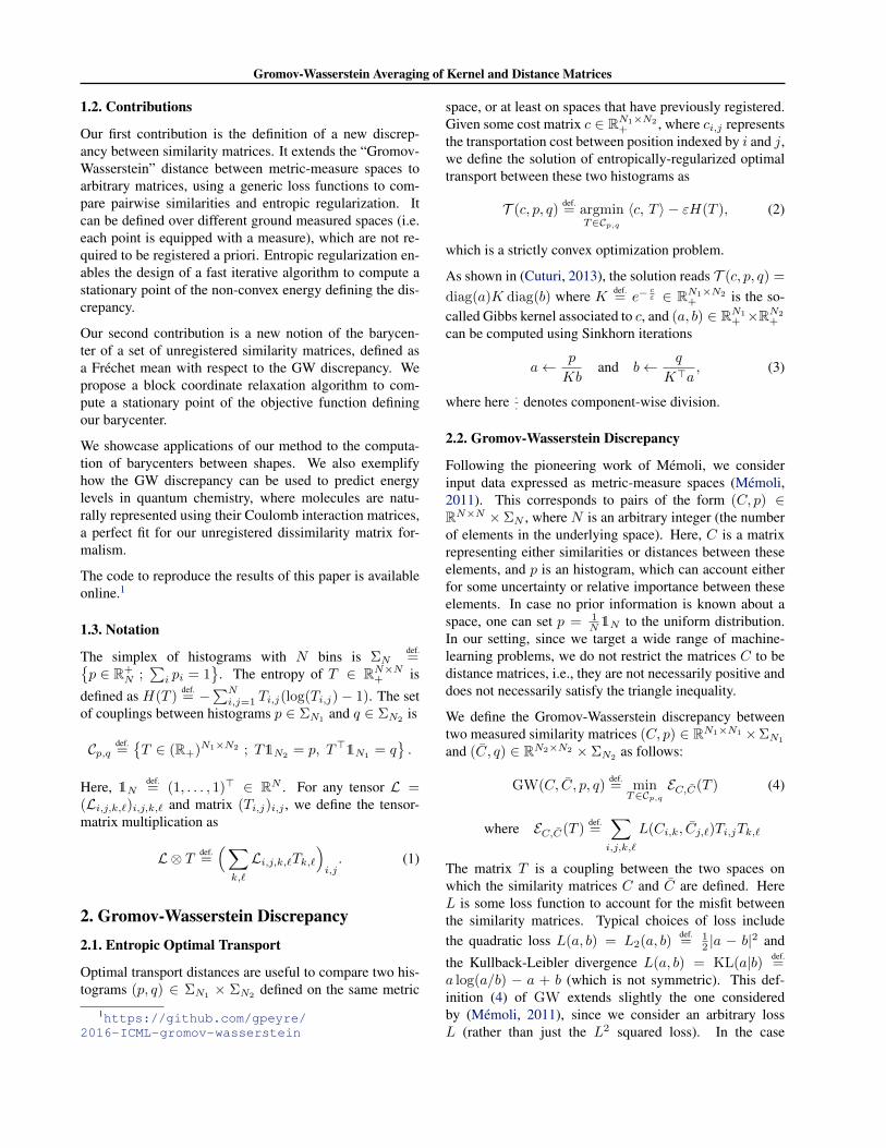
Gromov-Wasserstein Averaging of Kernel and Distance Matrices Gabriel Peyr´ e GABRIEL. PEYRE@CEREMADE. DAUPHINE. FR CNRS and Univ. Paris-Dauphine, Pl. du M. De Lattre De Tassigny, 75775 Paris 16, FRANCE Marco Cuturi MCUTURI @I . KYOTO- U. AC. JP Kyoto University, 36-1 Yoshida-Honmachi, Sakyo-ku, Kyoto 606-8501, JAPAN Justin Solomon JSOLOMON@MIT. EDU Massachusetts Institute of Technology, Cambridge, MA 02139, USA Abstract This paper presents a new technique for comput- ing the barycenter of a set of distance or kernel matrices. These matrices, which define the inter- relationships between points sampled from indi- vidual domains, are not required to have the same size or to be in row-by-row correspondence. We compare these matrices using the softassign cri- terion, which measures the minimum distortion induced by a probabilistic map from the rows of one similarity matrix to the rows of another; this criterion amounts to a regularized version of the Gromov-Wasserstein (GW) distance between metric-measure spaces. The barycenter is then defined as a Fr´ echet mean of the input matri- ces with respect to this criterion, minimizing a weighted sum of softassign values. We provide a fast iterative algorithm for the resulting noncon- vex optimization problem, built upon state-of- the-art tools for regularized optimal transporta- tion. We demonstrate its application to the com- putation of shape barycenters and to the predic- tion of energy levels from molecular configura- tions in quantum chemistry. 1. Introduction Many classes of input data encountered in machine learn- ing are best expressed using either pairwise distance ma- trices or kernels. For instance, the atoms making up pro- teins and other molecules have no canonical orientation and hence are only known up to rigid motion; so, the geom- etry of a molecule might be better described by the pair- Proceedings of the 33 rd International Conference on Machine Learning, New York, NY, USA, 2016. JMLR: W&CP volume 48. Copyright 2016 by the author(s). wise distances between atoms rather than by their abso- lute positions. Kernel and covariance matrices from differ- ent datasets exhibit similar structure, since they define data points by their roles relative to the rest of a dataset rather than in any absolute sense. A major difficulty with this representation is that in many applications these matrices are not “registered” or “aligned,” meaning that there is no explicit correspondence between their rows and columns. This is the case for shapes that undergo pose variation, articulation or deformation. Even worse, in some cases, similarities are not defined over the same ground space. For example, different molecules may have varying numbers of atoms. This inconsistency yields matrices of varying dimensions. In this paper, we propose a theoretical and computa- tional framework for summarizing collections of unaligned distance or kernel matrices. Building upon the notion of Gromov-Wasserstein (GW) distances between metric- measure spaces (M´ emoli, 2007), we provide machinery for registering matrices of varying sizes while building inter- polants and barycenters inheriting structure from the in- puts. We also derive a fast regularized approximation scheme providing a practical and efficient way to recover these barycenters in practice. 1.1. Previous Work Countless techniques leverage matrices of distances or ker- nels to describe a dataset. While distances and kernels have opposite ordering—a large distance indicates small similarity—unless it is necessary to distinguish we will use the term “similarity matrix” to refer to any matrix contain- ing pairwise relationships. Aligning similarity matrices. Comparison of similar- ity matrices is challenging due to a lack of alignment. Mathematically, they only define the intrinsic structure
-
Upload
duongnguyet -
Category
Documents
-
view
231 -
download
0
Transcript of Gromov-Wasserstein Averaging of Kernel and Distance …proceedings.mlr.press/v48/peyre16.pdf ·...

Gromov-Wasserstein Averaging of Kernel and Distance Matrices
Gabriel Peyre [email protected]
CNRS and Univ. Paris-Dauphine, Pl. du M. De Lattre De Tassigny, 75775 Paris 16, FRANCE
Marco Cuturi [email protected]
Kyoto University, 36-1 Yoshida-Honmachi, Sakyo-ku, Kyoto 606-8501, JAPAN
Justin Solomon [email protected]
Massachusetts Institute of Technology, Cambridge, MA 02139, USA
AbstractThis paper presents a new technique for comput-ing the barycenter of a set of distance or kernelmatrices. These matrices, which define the inter-relationships between points sampled from indi-vidual domains, are not required to have the samesize or to be in row-by-row correspondence. Wecompare these matrices using the softassign cri-terion, which measures the minimum distortioninduced by a probabilistic map from the rowsof one similarity matrix to the rows of another;this criterion amounts to a regularized version ofthe Gromov-Wasserstein (GW) distance betweenmetric-measure spaces. The barycenter is thendefined as a Frechet mean of the input matri-ces with respect to this criterion, minimizing aweighted sum of softassign values. We provide afast iterative algorithm for the resulting noncon-vex optimization problem, built upon state-of-the-art tools for regularized optimal transporta-tion. We demonstrate its application to the com-putation of shape barycenters and to the predic-tion of energy levels from molecular configura-tions in quantum chemistry.
1. IntroductionMany classes of input data encountered in machine learn-ing are best expressed using either pairwise distance ma-trices or kernels. For instance, the atoms making up pro-teins and other molecules have no canonical orientation andhence are only known up to rigid motion; so, the geom-etry of a molecule might be better described by the pair-
Proceedings of the 33 rd International Conference on MachineLearning, New York, NY, USA, 2016. JMLR: W&CP volume48. Copyright 2016 by the author(s).
wise distances between atoms rather than by their abso-lute positions. Kernel and covariance matrices from differ-ent datasets exhibit similar structure, since they define datapoints by their roles relative to the rest of a dataset ratherthan in any absolute sense.
A major difficulty with this representation is that inmany applications these matrices are not “registered” or“aligned,” meaning that there is no explicit correspondencebetween their rows and columns. This is the case for shapesthat undergo pose variation, articulation or deformation.Even worse, in some cases, similarities are not defined overthe same ground space. For example, different moleculesmay have varying numbers of atoms. This inconsistencyyields matrices of varying dimensions.
In this paper, we propose a theoretical and computa-tional framework for summarizing collections of unaligneddistance or kernel matrices. Building upon the notionof Gromov-Wasserstein (GW) distances between metric-measure spaces (Memoli, 2007), we provide machinery forregistering matrices of varying sizes while building inter-polants and barycenters inheriting structure from the in-puts. We also derive a fast regularized approximationscheme providing a practical and efficient way to recoverthese barycenters in practice.
1.1. Previous Work
Countless techniques leverage matrices of distances or ker-nels to describe a dataset. While distances and kernelshave opposite ordering—a large distance indicates smallsimilarity—unless it is necessary to distinguish we will usethe term “similarity matrix” to refer to any matrix contain-ing pairwise relationships.
Aligning similarity matrices. Comparison of similar-ity matrices is challenging due to a lack of alignment.Mathematically, they only define the intrinsic structure

Gromov-Wasserstein Averaging of Kernel and Distance Matrices
of a dataset, which remains unchanged e.g. under rota-tion, translation, and isometric motion. More concretely,there is unlikely to be a canonical ordering of the rows orcolumns of similarity matrices, and removing or adding afew rows/columns may not significantly affect the struc-ture. Automatic computation of a map aligning two sim-ilarity matrices is itself a challenging problem; our workis fairly unique in that we simultaneously compute such analignment while solving an optimization problem over suchmatrices.
Matching rows of similarity matrices usually becomes aquadratic assignment problem (Loiola et al., 2007), whichis NP-hard. For the specific case of aligning similarity ma-trices derived from pairwise distances in a metric space(e.g., geodesic distances along a surface), a well-knowninstance of this matching problem is computation of theGromov-Hausdorff distance (Gromov, 2001), which wasapplied to matching in (Memoli, 2007).
To relax the matching problem to a continuous—butstill non-convex—optimization problem, the seminal workof Memoli considers matching between metric-measurespaces, incorporating a probability distribution on theground space that can account for some form of uncer-tainty (Memoli, 2011). The geodesic properties of this“space of metric spaces” are considered in (Sturm, 2012).The recent work (Hendrikson, 2016) showcases the appli-cation of the corresponding Gromov-Wasserstein distanceto clustering of biological and social networks. It is possi-ble to further relax this formulation to a quadratic (Aflaloet al., 2015) or semidefinite (Kezurer et al., 2015) convexprogram, although this relaxation can fail if the input simi-larity matrices exhibit symmetries.
Rather than mixing the possible symmetric maps, we em-brace the nonconvexity of the original problem and opti-mize quadratic matching objectives directly. After regu-larization, our matching subroutine resembles “softassignquadratic assignment” (Rangarajan et al., 1999; Gold &Rangarajan, 1996). We extend their iterations to gen-eral loss functions and to more advanced machine learn-ing problems than nearest-neighbor search, in particularbarycenter computation. We additionally leverage the factthat GW can compare arbitrary matrices, not just pairwisedistances, making our machinery applicable to a broaderrange of tasks. The mapping component of our algorithmcan be considered a generalized version of the method re-cently proposed in (Solomon et al., 2016).
Averaging similarity matrices. The design of an “aver-age” or barycenter of similarity matrices is informed by twoprimary factors: A measure of discrepancy between simi-larity matrices and a definition of a mean. We will GWdistances to define discrepancies, so our remaining task is
to define what it means to compute a barycenter.
Even when similarity matrices are the same size and reg-istered, it may not make sense to average them arithmeti-cally. One natural way to define a mean or barycenter ofinputs (Cs)s is to minimize the sum
∑s λsd
2(C,Cs) overall possible C, where d is some notion of distance. Thisgeneralized notion of a mean is known as the Karcher orFrechet mean, which generalizes the notion of an averageto a wide class of metric spaces (Nielsen & Bhatia, 2012).
Frechet barycenters in Wasserstein space were proposedin (Agueh & Carlier, 2011). Several algorithms fortheir computation have been proposed including (Cuturi& Doucet, 2014; Benamou et al., 2015); these assume afixed ground distance metric. Our method, however, findsmore commonality with algorithms that compute Frechetmeans in the space of covariance or metric matrices. (Dry-den et al., 2009) considers several simple options for co-variance matrices, mostly with fixed alignment; their “Pro-crustes” mean provides one rudimentary strategy for align-ment. (Sra, 2011) defines a metric on registered positivedefinite kernel matrices that can be used for computingFrechet means.
Barycenter computation is a building block for many learn-ing methods. For instance, k-means clustering alter-nates between distances and barycenter computation. Thenearest-centroid classifier provides a similar approach toclassification (Manning et al., 2008).
Optimal transport (OT). OT (Villani, 2003) is a way tocompare probability distributions (histograms in the finite-dimensional case) defined over either the same groundspace or multiple pre-registered ground spaces. Themeans of comparison is a convex linear program optimiz-ing for a matching that moves the mass from one dis-tribution to the other with minimal cost. OT has beenapplied to machine learning problems including compar-ison of descriptors (Cuturi, 2013), k-means (Cuturi &Doucet, 2014), semi-supervised learning (Solomon et al.,2014), domain adaptation (Courty et al., 2014), designingloss functions (Frogner et al., 2015), low-rank approxima-tion (Seguy & Cuturi, 2015), and dictionary learning (Roletet al., 2016).
As highlighted above, GW-style matching extends OT tothe case when the ground spaces are not pre-registered,yielding a non-convex quadratic program to compute thetransport. The resulting transportation matrix can be un-derstood is a soft registration from one domain to the other.Our algorithm solves a entropically-regularized version ofthis quadratic program by extending recent advances in thecomputation of OT (Cuturi, 2013; Benamou et al., 2015).
Gromov-Wasserstein Averaging of Kernel and Distance Matrices
1.2. Contributions
Our first contribution is the definition of a new discrep-ancy between similarity matrices. It extends the “Gromov-Wasserstein” distance between metric-measure spaces toarbitrary matrices, using a generic loss functions to com-pare pairwise similarities and entropic regularization. Itcan be defined over different ground measured spaces (i.e.each point is equipped with a measure), which are not re-quired to be registered a priori. Entropic regularization en-ables the design of a fast iterative algorithm to compute astationary point of the non-convex energy defining the dis-crepancy.
Our second contribution is a new notion of the barycen-ter of a set of unregistered similarity matrices, defined asa Frechet mean with respect to the GW discrepancy. Wepropose a block coordinate relaxation algorithm to com-pute a stationary point of the objective function definingour barycenter.
We showcase applications of our method to the computa-tion of barycenters between shapes. We also exemplifyhow the GW discrepancy can be used to predict energylevels in quantum chemistry, where molecules are natu-rally represented using their Coulomb interaction matrices,a perfect fit for our unregistered dissimilarity matrix for-malism.
The code to reproduce the results of this paper is availableonline.1
1.3. Notation
The simplex of histograms with N bins is ΣNdef.={
p ∈ R+N ;
∑i pi = 1
}. The entropy of T ∈ RN×N+ is
defined as H(T )def.= −
∑Ni,j=1 Ti,j(log(Ti,j)− 1). The set
of couplings between histograms p ∈ ΣN1and q ∈ ΣN2
is
Cp,qdef.={T ∈ (R+)N1×N2 ; T1N2
= p, T>1N1= q}.
Here, 1Ndef.= (1, . . . , 1)> ∈ RN . For any tensor L =
(Li,j,k,`)i,j,k,` and matrix (Ti,j)i,j , we define the tensor-matrix multiplication as
L ⊗ T def.=(∑k,`
Li,j,k,`Tk,`)i,j. (1)
2. Gromov-Wasserstein Discrepancy2.1. Entropic Optimal Transport
Optimal transport distances are useful to compare two his-tograms (p, q) ∈ ΣN1 × ΣN2 defined on the same metric
1https://github.com/gpeyre/2016-ICML-gromov-wasserstein
space, or at least on spaces that have previously registered.Given some cost matrix c ∈ RN1×N2
+ , where ci,j representsthe transportation cost between position indexed by i and j,we define the solution of entropically-regularized optimaltransport between these two histograms as
T (c, p, q)def.= argmin
T∈Cp,q〈c, T 〉 − εH(T ), (2)
which is a strictly convex optimization problem.
As shown in (Cuturi, 2013), the solution reads T (c, p, q) =
diag(a)K diag(b) where K def.= e−
cε ∈ RN1×N2
+ is the so-called Gibbs kernel associated to c, and (a, b) ∈ RN1
+ ×RN2+
can be computed using Sinkhorn iterations
a← p
Kband b← q
K>a, (3)
where here ·· denotes component-wise division.
2.2. Gromov-Wasserstein Discrepancy
Following the pioneering work of Memoli, we considerinput data expressed as metric-measure spaces (Memoli,2011). This corresponds to pairs of the form (C, p) ∈RN×N ×ΣN , where N is an arbitrary integer (the numberof elements in the underlying space). Here, C is a matrixrepresenting either similarities or distances between theseelements, and p is an histogram, which can account eitherfor some uncertainty or relative importance between theseelements. In case no prior information is known about aspace, one can set p = 1
N 1N to the uniform distribution.In our setting, since we target a wide range of machine-learning problems, we do not restrict the matrices C to bedistance matrices, i.e., they are not necessarily positive anddoes not necessarily satisfy the triangle inequality.
We define the Gromov-Wasserstein discrepancy betweentwo measured similarity matrices (C, p) ∈ RN1×N1 ×ΣN1
and (C, q) ∈ RN2×N2 × ΣN2as follows:
GW(C, C, p, q)def.= min
T∈Cp,qEC,C(T ) (4)
where EC,C(T )def.=∑i,j,k,`
L(Ci,k, Cj,`)Ti,jTk,`
The matrix T is a coupling between the two spaces onwhich the similarity matrices C and C are defined. HereL is some loss function to account for the misfit betweenthe similarity matrices. Typical choices of loss includethe quadratic loss L(a, b) = L2(a, b)
def.= 1
2 |a − b|2 and
the Kullback-Leibler divergence L(a, b) = KL(a|b) def.=
a log(a/b) − a + b (which is not symmetric). This def-inition (4) of GW extends slightly the one consideredby (Memoli, 2011), since we consider an arbitrary lossL (rather than just the L2 squared loss). In the case

Gromov-Wasserstein Averaging of Kernel and Distance Matrices
L = L2, (Memoli, 2011) proves that GW1/2 defines a dis-tance on the space of metric measure spaces quotiented bymeasure-preserving isometries.
Introducing the 4-way tensor
L(C, C)def.= (L(Ci,k, Cj,`))i,j,k,`,
we notice that
EC,C(T ) = 〈L(C, C)⊗ T, T 〉,
where ⊗ denotes the tensor-matrix multiplication (1).
The following proposition shows how to computeL(C, C) ⊗ T efficiently for a general class of loss func-tions:
Proposition 1. If the loss can be written as
L(a, b) = f1(a) + f2(b)− h1(a)h2(b) (5)
for functions (f1, f2, h1, h2), then, for any T ∈ Cp,q ,
L(C, C)⊗ T = cC,C − h1(C)Th2(C)>. (6)
where cC,Cdef.= f1(C)p1>N2
+1N1q>f2(C)> is independent
of T .
Proof. Under hypothesis (5), formula (1) shows that onehas the decomposition L(C, C)⊗ T = A+B + C where
Ai,j =∑k
f1(Ci,k)∑`
Tk,` = (f1(C)(T1))i
Bi,j =∑`
f2(Cj,`)∑k
Tk,` = (f2(C)(T>1))j
Ci,j =∑k
h1(Ci,k)∑`
h2(Cj,`)Tk,`
which is equal to (h1(C)(h1(C)T>)>)i,j .
Remark 1 (Computational complexity). Formula (6) showsthat for this class of losses, one can compute L(C, C)⊗ Tefficiently inO(N2
1N2+N22N1) operations, using only ma-
trix/matrix multiplications, instead of the O(N21N
22 ) com-
plexity of the naıve implementation of formula (1).Remark 2 (Special cases). The square loss L = L2 sat-isfies (5) for f1(a) = a2, f2(b) = b2, h1(a) = a andh2(b) = 2b. The KL loss L = KL satisfies (5) for f1(a) =a log(a)− a, f2(b) = b, h1(a) = a and h2(b) = log(b).
2.3. Entropic Gromov-Wasserstein Discrepancy
We consider the following entropic approximation of theinitial GW formulation (4)
GWε(C, C, p, q)def.= min
T∈Cp,qEC,C(T )− εH(T ). (7)
This is a non-convex optimization problem. We proposeto use projected gradient descent, where both the gradientstep and the projection are computed according to the KLmetric.
Iterations of this algorithm are given by
T ← ProjKLCp,q
(T � e−τ(∇EC,C(T )−ε∇H(T ))
), (8)
where τ > 0 is a small enough step size, and the KL pro-jector of any matrix K is
ProjKLCp,q (K)
def.= argmin
T ′∈Cp,qKL(T ′|K).
Proposition 2. In the special case τ = 1/ε, iteration (8)reads
T ← T (L(C, C)⊗ T, p, q). (9)
Proof. As shown in (Benamou et al., 2015), the projectionis nothing else than the solution to the regularized transportproblem (2), hence
ProjKLCp,q (K) = T (−ε log(K), p, q).
One also has
∇EC,C(T )− ε∇H(T ) = L(C, C)⊗ T + ε log(T ).
Re-arranging the terms in (8), one obtains, in the specialcase τε = 1, the desired formula.
Iteration (9) defines a surprisingly simple algorithm, inwhich each update of T involves a Sinkhorn projection.Remark 3 (Convergence). Using (Bot et al., 2015) (seeTheorem 12), iterations (8) are guaranteed to converge pro-vided that τ is chosen small enough, τ < τmax. Unfor-tunately, in general, one does not have τmax > 1/ε, sothat the step size τ = 1/ε advocated by Proposition 2 isnot covered by the theory. However, we found that usingτ = 1/ε always leads to a converging sequence of T , andthat this works well in practice. Note that when L = L2,this recovers the “softassign quadratic assignement” algo-rithms defined in (Rangarajan et al., 1999; Gold & Ran-garajan, 1996). The convergence proof (Rangarajan et al.,1999), however, only ensures convergence of the functionalvalues (not of the iterates) and also only applies when thefunction being minimized in (7) is convex, which is not thecase for arbitrary matrices (C,Cs).
3. Gromov-Wasserstein Barycenters3.1. Gromov-Wasserstein Barycenters
We define Gromov-Wasserstein barycenters of measuredsimilarity matrices (Cs)
Ss=1, where Cs ∈ RNs×Ns , using

Gromov-Wasserstein Averaging of Kernel and Distance Matrices
a Frechet mean formulation:
minC∈RN×N
∑s
λs GWε(C,Cs, p, ps). (10)
In this section, for simplicity, we assume that the basehistograms (ps)s and the histogram p associated to thebarycenter are known and fixed. Note in particular thatthe size (N,N) of the targeted barycenter matrix shouldbe fixed by the user. It is straightforward to extend the ex-position as well as the optimization algorithm to the settingwhere p is unknown and included as an optimization vari-able.
This barycenter can be reformulated by re-introducing cou-plings
minC,(Ts)s
∑s
λs (EC,Cs(Ts)− εH(Ts)) (11)
subject to the constraints that for all s, Ts ∈ Cp,ps ⊂RN×Ns+ .
Note that if L is convex with respect to its first variable, thisproblem is convex with respect to C but not with respect to(Ts)s (it is a quadratic but not necessarily positive problemwith respect to the (Ts)s).
We propose to minimize (11) using a block coordinate re-laxation, i.e. iteratively minimizing with respect to the cou-plings (Ts)s and to the metric C.
Minimization with respect to (Ts)s. The optimizationproblem (10) over (Ts)s alone decouples as S independentGWε optimizations
∀ s, minTs∈Cp,ps
EC,Cs(Ts)− εH(Ts).
A stationary point of this optimization problem can be com-puted using the optimization algorithm detailed in Sec-tion 2.3.
Minimization with respect to C. For given (Ts), theminimization with respect to C reads
minC
∑s
λs〈L(C,Cs)⊗ T, T 〉. (12)
The following proposition shows, for a large class of losses,how to compute the global minimizer in closed form.
Proposition 3. If L satisfies (5) and f ′1/h′1 is invertible,
then the solution to (12) reads
C =
(f ′1h′1
)−1(∑s λsT
>s h2(Cs)Tspp>
), (13)
where we assume the normalization∑s λs = 1.
Proof. Using relation (6), the functional to be minimizedreads∑s
λs〈f1(C)p1>+1p>s f2(Cs)−h1(C)Tsh2(Cs)>, Ts〉.
The first order optimality condition for this optimiza-tion problem thus reads f ′1(C) � (pp>) = h′1(C) �∑s λsTsh2(Cs)T
>s , which gives the desired formula.
The intuition underlying formula (13) is clear: EachT>s h2(Cs)Ts is a “realigned” matrix where Ts acts asa fuzzy permutation (optimal transportation coupling) ofboth rows and columns of the distance matrix Cs. Theserealigned metric are then averaged, where the precise no-tion of “averaging” depends on the loss L.
Barycenters of PSD kernels using L2 loss. For thesquare loss L = L2, the update (13) becomes
C ← 1
pp>
∑s
λsT>s CsTs. (14)
This formula highlights an important property of themethod:
Proposition 4. For L = L2, if the (Cs)s are positivesemidefinite (PSD) matrices, the iteratesC produced by thealgorithm are also PSD.
Proof. Formula (14) shows that the update of Ccorresponds to a linear averaging of the matrices(diag(1/p)T>s CsTs diag(1/p))s, which are all PSD sincethe matrices (Cs)s are.
This proposition implies, since the SDP cone is a closed set,that the output of our barycenter algorithm at convergenceis an SDP kernel.
Barycenters of infinitely divisible kernels using KL loss.For the KL loss L = KL, the update (13) similar, but witha geometric mean in place of an arithmetic mean
C ← exp
(1
pp>
∑s
λsT>s log(Cs)Ts
). (15)
The following proposition shows that this loss is partic-ularly attractive for averaging infinitely divisible kernels.Recall that C ∈ RN×N is infinitely divisible if and only ifU = log(C) is a conditionally positive semidefinite ker-nel, i.e. for all x ∈ RN such that 〈x, 1N 〉 = 0, then〈Ux, x〉 > 0.
Proposition 5. For L = KL, if the (Cs)s are infinitelydivisible kernels, the iterates C produced by the algorithmare also infinitely divisible.

Gromov-Wasserstein Averaging of Kernel and Distance Matrices
Algorithm 1 Computation of GWε barycenters.Input: (Cs, ps)s, pInitialize C.repeat
// minimize over (Ts)sfor s = 1 to S do
Initialize Ts.repeat
// compute cs = L(C,Cs)⊗ Ts using (6).cs ← f1(C)+ f2(Cs)> − h1(C)Tsh2(Cs)>
// Sinkhorn iterations (3) to compute T (cs, p, q)Initialize a← 1, set K ← e−cs/ε.repeata← p
Kb , b←q
K>a.
until convergenceUpdate Ts ← diag(a)K diag(b).
until convergenceend for// minimize over C using (13).
C ←(f ′1h′1
)−1 (∑s λsT
>s h2(Cs)Tspp>
)until convergence
Proof. According to formula (15), one has to show thatU
def.=∑s λs diag(1/p)T>s UsTs diag(1/p) is conditionally
PSD prodived that the Us matrices are. This is indeedthe case, because, for any x such that 〈x, 1N 〉 = 0, onehas 〈Ux, x〉 =
∑s λs〈Usxs, xs〉 where xs
def.= Ts
xp , and
since 〈xs, 1Ns〉 = 〈xp , T>s 1Ns〉 = 〈xp , p〉 = 0, one has
〈Usxs, xs〉 > 0 so that 〈Ux, x〉 > 0, which proves theresult.
This proposition implies, since the cone of infinitely divisi-ble kernels is a closed set, that the output of our barycenteralgorithm at convergence is infinitely divisible.
A important example of infinitely divisible kernels is given
by the form C = e−D2
σ2 , where Di,j = ||xi− xj || is the Eu-clidean distance matrix between points (xi)i, and σ > 0is a bandwidth parameter that controls the “locality” of
the resulting kernel. One verifies that KL(e−D2
σ2 |e−D2
σ2 ) =1
2σ4 ||D2 − D2||2 + o(1/σ4), so that in the regime of largebandwidth σ → +∞, using the KL loss in conjunctionwith this class of kernels becomes equivalent to using theL2 loss between squared Euclidean matrices. A similar re-sult in fact holds for any smooth Bregman divergence loss.
Pseudocode. Algorithm 1 details the steps of the opti-mization technique. Note that it makes use of three nestediterations: (i) blockwise coordinate descent on (Ts)s andC, (ii) projected gradient descent on each Ts, and (iii)Sinkhorn iterations to compute the projection.
Figure 1. Barycenters of point clouds from MNIST digits; sampleinput data clouds are shown on the left, and an MDS embeddingof the barycenter distance matrix is shown on the right.
Figure 2. Barycenter example for shape data from (Thakoor et al.,2007).
4. Experiments4.1. Point Clouds
Embedded barycenters. Figure 1 provides an exampleillustrating the behavior of our GW barycenter approxima-tion. In this experiment, we extract 500 point clouds ofhandwritten digits from the dataset (LeCun et al., 1998),rotated arbitrarily in the plane. We represent each digit asa symmetric Euclidean distance matrix and optimize for a500× 500 barycenter using Algorithm 1 (uniform weights,ε = 1 × 10⁻³); notice that most of the input point cloudsconsist of fewer than 500 points. We then visualize thebarycenter matrix as a point cloud in the plane using multi-dimensional scaling (MDS). Each digit is colored by trans-ferring RGB values from the barycenter point cloud usingthe computed map T .
This experiment illustrates a few properties of our algo-rithm. Most prominently, note that the input digits are ro-tated arbitrarily, which—unlike tools based on classicaloptimal transportation—does not affect the computation ofthe barycenter. Also, to avoid bias in this experiment weinitialize C as a random matrix, and yet our nonconvex op-timization algorithm still reaches a meaningful barycenter.
Figure 2 illustrates a similar experiment on the 2D shapedata from (Thakoor et al., 2007). This second experimentillustrates some additional properties of our barycenters.Interestingly, even though we do not impose curve topol-

Gromov-Wasserstein Averaging of Kernel and Distance Matrices
Figure 3. Progressive interpolation (xt)1t=0 between two shapes
(x0, x1) using GW barycenters.
ogy on the barycenter, the final MDS embedding has one-dimensional structure. The barycenter is also resilient tonoise in the computed map from individual examples, e.g.the bones in the first row.
Regularization. Figure bellow illustrates the de-pendence of our barycenter on the regularizer ε.
ε = 1.5× 10⁻³ ε = 4× 10⁻³ ε = 8× 10⁻³ ε = 1.6× 10⁻²ε = 3.2× 10⁻²
It shows the barycenter from a test in Figure 2 for increas-ing values of ε. When ε is small, the embedded barycentermost closely resembles the input data. As ε increases,the barycenters become smoother, with the advantage ofhigher resilience to noise and fewer iterations needed foroptimization.
Clustering. The figure onthe right illustrates the in-corporation of our barycentertechnique into a larger ma-chine learning pipeline. Itshows results of a k-meansunsupervised clustering of250 handwritten characters.
1234
0
0
50
In this example, we construct a dataset with 50 point cloudsfrom each of digits 0 to 4 from the example in Figure 1. Wethen cluster the point clouds by representing them as pair-wise distance matrices and applying the k-means algorithm(k = 5), with k-means++ initialization (Arthur & Vassilvit-skii, 2007). We underscore that each handwritten characteris represented using an unaligned point cloud with varyingnumbers of points.
Each row in the figure corresponds to a different character,and each column corresponds to a different cluster center(MDS embedding shown above the table). Color is propor-tional to the number of data points assigned to each clus-ter. Even without supervision, this rudimentary techniquefor clustering finds meaningful clusters of handwritten dig-its from the dataset. All the “1” digits are clustered cor-
Figure 4. Upper part: comparison between interpolation using L2
loss and KL loss. Lower part: comparison between interpolationusing pairwise Euclidean and inner geodesic distances.
rectly. Digits 2 and 4 are mixed considerably in the com-puted clustering, reflecting the wide variety of handwrittenstyles for these two digits.
Shape interpolation. Figure 3 shows an application ofthe computation of GW barycenters between S = 2 inputmatrices two perform shape interpolation. The input matri-ces (C1, C2) ∈ (RN×N )2 are Euclidean distance matricesof two input planar clouds (xs,i)i for s ∈ {1, 2} uniformlysampled inside a shape, so that we use p1 = p2
1N 1N .
This means that Cs,i,jdef.= ||xs,i − xs,j || for s ∈ {1, 2} and
i, j = 1, . . . , N . The interpolation is achieved by first com-puting a barycenter matrix Ct minimizing (10) with ouroptimization algorithm, for λ = (t, 1 − t), t ∈ [0, 1], us-ing the Euclidean loss L = L2. A barycentric point cloudxt = (xt,i)
Ni=1 is then reconstructed using SMACOF multi-
dimensional scaling (MDS), which amounts to computinga local minimizer of
∑i,j |Ct,i,j − ||xt,i − xt,j |||2 with re-
spect to (xt,i)i. This local minimizer xt is computed by agradient descent scheme, initialized with x1.
L2 vs. KL losses. Figure 4, upper part, shows a compar-ison of the same interpolation as those computed in Fig-ure 3, computed with two different losses. Row #1 showsbarycenters of the distance matrices Cs,i,j = ||xs,i − xs,j ||,for s ∈ {1, 2}, using the squared Euclidean loss L = L2
as in the previous paragraph. The display is obtainedby applying SMACOF MDS to the barycenter matrix Ct.Row #2 shows barycenter of the infinitely divisible kernelsCs,i,j = exp(−||xs,i − xs,j ||2/σ2), for s = {1, 2}, usingthe Kullback-Leibler loss L =KL, and a bandwidth σ = 1(for point clouds in the unit square). The display is thenobtained by applying SMACOF MDS to
√−σ log(Ct).
The KL interpolation produces less regular interpolationbecause it imposes only local constraints at the scale of thebandwidth.

Gromov-Wasserstein Averaging of Kernel and Distance Matrices
Euclidean vs. Geodesic distance matrices. Euclideanpairwise distance, though simple to compute and to ma-nipulate, fail to capture the intrinsic geometry of shapes,and thus leads to physically unrealistic shape interpolation,that ignore in particular articulation. Figure 4, lower part,shows how this issue can be in large part alleviated by re-placing the extrinsic Euclidean distance Cs,i,j = ||xs,i −xs,j || for s ∈ {1, 2} by the inner geodesic distance (i.e. thelength of the shortest path joining xs,i to xs,j while stayinginside the shape). Note that, because the corresponding dis-tance is not Euclidean anymore, the SMACOF MDS onlyproduces an approximate embedding, the so-called bendinginvariant (Elad & Kimmel, 2003) used to perform isomeric-invariant shape recognition.
4.2. Quantum chemistry
To demonstrate the interest of the Gromov-Wasserstein dis-crepancy, we consider its application to a regression prob-lem on molecules. Several recent works (Rupp et al., 2012;Hansen et al., 2013) have proposed to predict atomiza-tion energies for molecules using descriptors of labeledmolecules, rather than estimating them through expensivenumerical simulations. (Rupp et al., 2012) proposed in par-ticular to represent each molecule in the qm7 dataset of or-ganic 7165 molecules through its so-called “Coulomb ma-trix,” which we describe next.
Coulomb matrices. For a molecule s with Ns atoms,each described by a relative location ri ∈ R3 in spaceand a nuclear charge Zi, Rupp et al. proposed to form theNs×Ns matrix Cs with off-diagonal terms ZiZj/||ri−rj ||for 1 6 i 6= j 6 Ns, and diagonal terms 1
2Z2.4i . Al-
though this plays no major role in our analysis, we foundthat these 7165 Coulomb matrices are all infinitely divisiblepositive definite kernel matrices. Rupp et al. argue that theCoulomb matrix is a convenient descriptor for moleculesin the sense that it is invariant with respect to translationsand rotations by construction. It has, however, an importantweakness: Cs has an arbitrary ordering of the Ns atoms ins. As we explain next, this was addressed by Rupp et al. bycreating randomly permuted copies of these matrices.
Previous work. Because their approach requires manipu-lating matrices of the same size, Rupp et al. pad allNs×NsCoulomb matrices Cs with zeros to obtain 23×23 matrices(23 is the maximal number of atoms in a molecule in theqm7 database). To cope with the ordering problem, theyalso propose, as a representation for each molecule, to formseveral randomly permuted copies of Cs for each molecules (between 8 and 1000 in (Hansen et al., 2013)). (Hansenet al., 2013, Table 3) provide out-of-sample mean absoluteerror (MAE) predictions for several techniques using 5 foldcross-validation. We report some of them in Table 4.2.
Algorithm MAE RMSEk-nearest neighbors 71.54 95.97Linear regression 20.72 27.22
Gaussian kernel ridge regression 8.57 12.26Laplacian kernel ridge regression (8) 3.07 4.84Multilayer Neural Network (1000) 3.51 5.96
GW 3-nearest neighbors 10.83 29.27
Table 1. Mean-Absolute and Root Mean Squared errors for theatomization energy prediction in the qm7 database of 7165molecules. All results quoted from (Hansen et al., 2013, Table3) except ours. Number in between parenthesis stand for randomcopies used in the algorithm. Although the GW distance is notdirectly competitive performance-wise, this result shows that anacceptable performance on this task can be recovered exclusivelyusing simple metric tools.
Our approach. We propose to use the original Ns ×Ns Coulomb matrices Cs directly as inputs for ourGW distances. Namely, we compute a discrep-ancy between two molecules s, s′ that is exactlyGW(Cs, Cs′ ,1Ns/Ns,1Ns′/Ns′), using L = L2 and aregularization strength ε tuned heuristically on a subsetof 500 points of the database. Using a 3-nearest neigh-bor regression approach we obtain a MAE of 10.83 which,although not directly competitive with the best approachrecorded in (Hansen et al., 2013), it remarkable in the sensethat it is obtained with an extremely simple classifier. Ourresult contradicts thus the observation made by Hansenet al., p.3414, that This [poor performance of k-nn] indi-cates that there are meaningful linear relations betweenphysical quantities in the system and that it is insufficientto simply look up the most similar molecules (as k- nearestneighbors does). The k-nearest neighbors approach fails tocreate a smooth mapping to the energies.
5. ConclusionThe Gromov-Wasserstein discrepancy measure is relevantto countless problems in machine learning for which theprimary role of a given data point is defined relative to othermembers of the dataset. After introducing an entropic reg-ularizer to the problem, we in particular find that GW is notonly theoretically attractive but also a practical tool with anefficient and easily-implemented non-convex optimizationscheme. Our approach highlights the fact that using un-registered similarity matrices as features in machine learn-ing problems is fruitful in many contexts. GW providesa natural framework for manipulation of these matrices, aswe demonstrate on classification, clustering, and regressiontasks for shapes and molecules. We suspect this elegant andefficient solution to extend to many other problem instancesendowed with natural geometric structure.

Gromov-Wasserstein Averaging of Kernel and Distance Matrices
Acknowledgements The work of G. Peyre has been sup-ported by the European Research Council (ERC projectSIGMA-Vision). J. Solomon acknowledges the support ofthe NSF Mathematical Sciences Postdoctoral Research Fel-lowship (award number 1502435).
ReferencesAflalo, Yonathan, Bronstein, Alexander, and Kimmel, Ron. On
convex relaxation of graph isomorphism. Proc. NationalAcademy of Sci., 112(10):2942–2947, 2015.
Agueh, Martial and Carlier, Guillaume. Barycenters in theWasserstein space. SIAM Journal on Mathematical Analysis,43(2):904–924, 2011.
Arthur, David and Vassilvitskii, Sergei. K-means++: The advan-tages of careful seeding. In Proc. SODA, pp. 1027–1035, 2007.
Benamou, Jean-David, Carlier, Guillaume, Cuturi, Marco, Nenna,Luca, and Peyre, Gabriel. Iterative Bregman projections forregularized transportation problems. SIAM J. Sci. Comp., 37(2):A1111–A1138, 2015.
Bot, Radu Ioan, Csetnek, Erno Robert, and Laszlo, Szilard Csaba.An inertial forward–backward algorithm for the minimizationof the sum of two nonconvex functions. EURO J. Comp. Op-tim., pp. 1–23, 2015.
Courty, Nicolas, Flamary, Remi, and Tuia, Devis. Domain adap-tation with regularized optimal transport. In Machine Learningand Knowledge Discovery in Databases, pp. 274–289. 2014.
Cuturi, Marco. Sinkhorn distances: Lightspeed computation ofoptimal transportation. In Proc. NIPS, volume 26, pp. 2292–2300. 2013.
Cuturi, Marco and Doucet, Arnaud. Fast computation of Wasser-stein barycenters. In Proc. ICML, volume 32, 2014.
Dryden, Ian L, Koloydenko, Alexey, and Zhou, Diwei. Non-Euclidean statistics for covariance matrices, with applicationsto diffusion tensor imaging. The Annals of Applied Statistics,pp. 1102–1123, 2009.
Elad, Asi and Kimmel, Ron. On bending invariant signatures forsurfaces. IEEE Tr. on PAMI, 25(10):1285–1295, 2003.
Frogner, Charlie, Zhang, Chiyuan, Mobahi, Hossein, Araya,Mauricio, and Poggio, Tomaso. Learning with a Wassersteinloss. In Advances in Neural Information Processing Systems,volume 28, pp. 2044–2052. 2015.
Gold, Steven and Rangarajan, Anand. A graduated assignmentalgorithm for graph matching. PAMI, 18(4):377–388, April1996.
Gromov, Mikhail. Metric Structures for Riemannian and Non-Riemannian Spaces. Progress in Math. Birkhauser, 2001.
Hansen, Katja, Montavon, Gregoire, Biegler, Franziska, Fazli,Siamac, Rupp, Matthias, Scheffler, Matthias, Von Lilienfeld,O Anatole, Tkatchenko, Alexandre, and Mller, Klaus-Robert.Assessment and validation of machine learning methods forpredicting molecular atomization energies. Journal of Chemi-cal Theory and Computation, 9(8):3404–3419, 2013.
Hendrikson, Reigo. Using Gromov-Wasserstein distance to ex-plore sets of networks. In University of Tartu, Master Thesis,2016.
Kezurer, Itay, Kovalsky, Shahar Z., Basri, Ronen, and Lipman,Yaron. Tight relaxation of quadratic matching. CGF, 2015.
LeCun, Yann, Bottou, Leon, Bengio, Yoshua, and Haffner,Patrick. Gradient-based learning applied to document recog-nition. Proceedings of the IEEE, 86(11):2278–2324, 1998.
Loiola, Eliane Maria, de Abreu, Nair Maria Maia, Boaventura-Netto, Paulo Oswaldo, Hahn, Peter, and Querido, Tania. Asurvey for the quadratic assignment problem. European J. Op-erational Research, 176(2):657–690, 2007.
Manning, Christopher D., Raghavan, Prabhakar, and Schutze,Hinrich. Introduction to Information Retrieval. CambridgeUniversity Press, 2008.
Memoli, Facundo. On the use of Gromov–Hausdorff distances forshape comparison. In Symposium on Point Based Graphics, pp.81–90. 2007.
Memoli, Facundo. Gromov–Wasserstein distances and the metricapproach to object matching. Foundations of Comp. Math., 11(4):417–487, 2011.
Nielsen, Frank and Bhatia, Rajendra. Matrix Information Geom-etry. Springer, 2012.
Rangarajan, Anand, Yuille, Alan, and Mjolsness, Eric. Conver-gence properties of the softassign quadratic assignment algo-rithm. Neural Comput., 11(6):1455–1474, August 1999.
Rolet, Antoine, Cuturi, Marco, and Peyre, Gabriel. Fast dictio-nary learning with a smoothed Wasserstein loss. In Proc. AIS-TATS’16, 2016.
Rupp, Matthias, Tkatchenko, Alexandre, Muller, Klaus-Robert,and Von Lilienfeld, O Anatole. Fast and accurate modeling ofmolecular atomization energies with machine learning. Physi-cal review letters, 108(5):058301, 2012.
Seguy, Vivien and Cuturi, Marco. Principal geodesic analysis forprobability measures under the optimal transport metric. In Ad-vances in Neural Information Processing Systems, pp. 3294–3302, 2015.
Solomon, Justin, Rustamov, Raif, Guibas, Leonidas, andButscher, Adrian. Earth mover’s distances on discrete surfaces.ACM Trans. Graph., 33(4):67:1–67:12, July 2014.
Solomon, Justin, Peyre, Gabriel, Kim, Vladimir, and Sra, Suvrit.Entropic metric alignment for correspondence problems. ACMTransactions on Graphics (TOG), 35(4), 2016.
Sra, Suvrit. Positive definite matrices and the S-divergence. arXivpreprint arXiv:1110.1773, 2011.
Sturm, Karl-Theodor. The space of spaces: curvature bounds andgradient flows on the space of metric measure spaces. Preprint1208.0434, arXiv, 2012.
Thakoor, Ninad, Gao, Jean, and Jung, Sungyong. Hidden Markovmodel-based weighted likelihood discriminant for 2-D shapeclassification. Trans. Image Proc., 16(11):2707–2719, 2007.
Villani, Cedric. Topics in Optimal Transportation. Graduate stud-ies in Math. AMS, 2003.